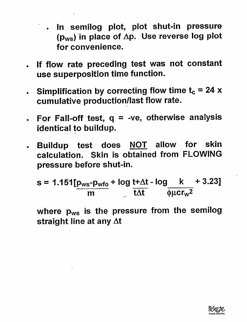
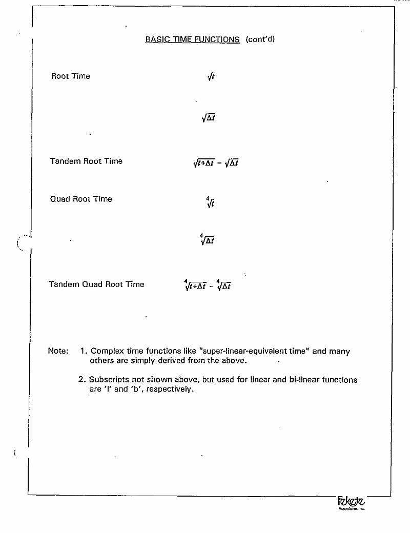
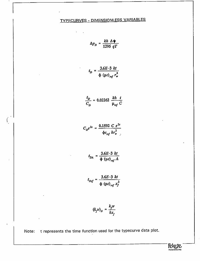
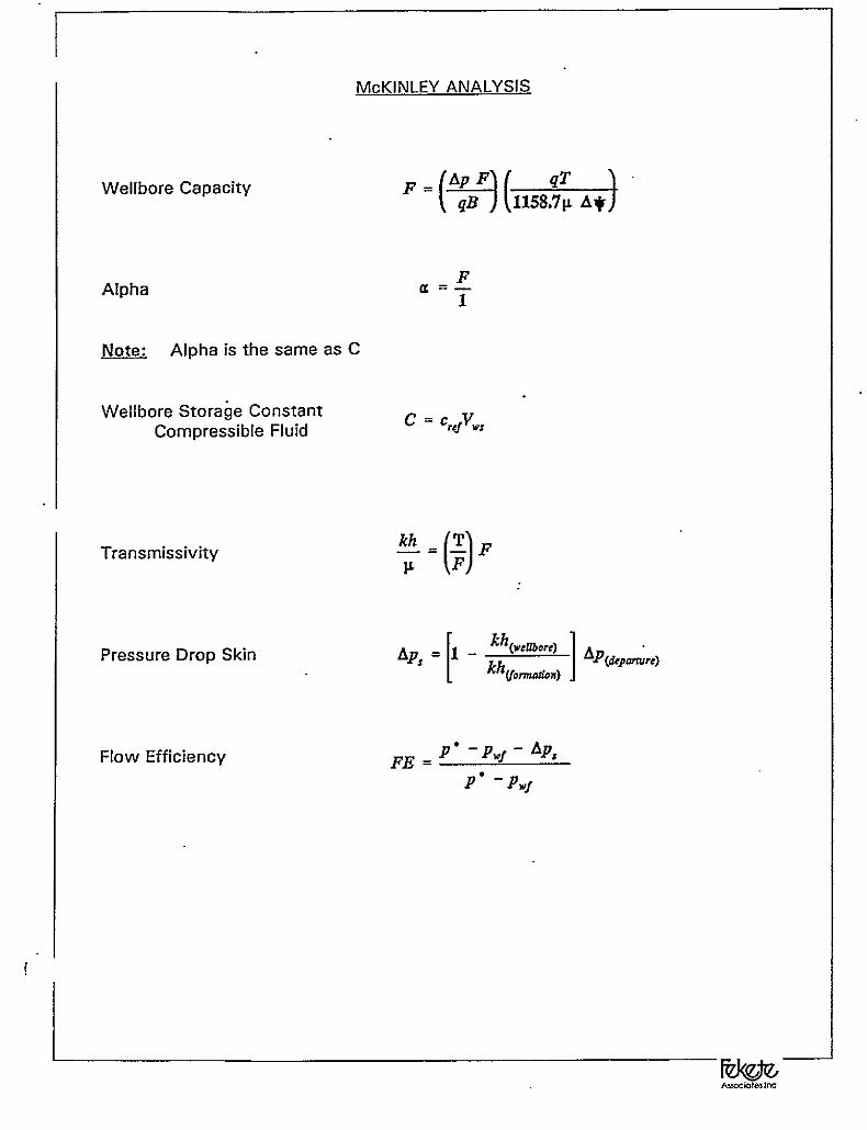
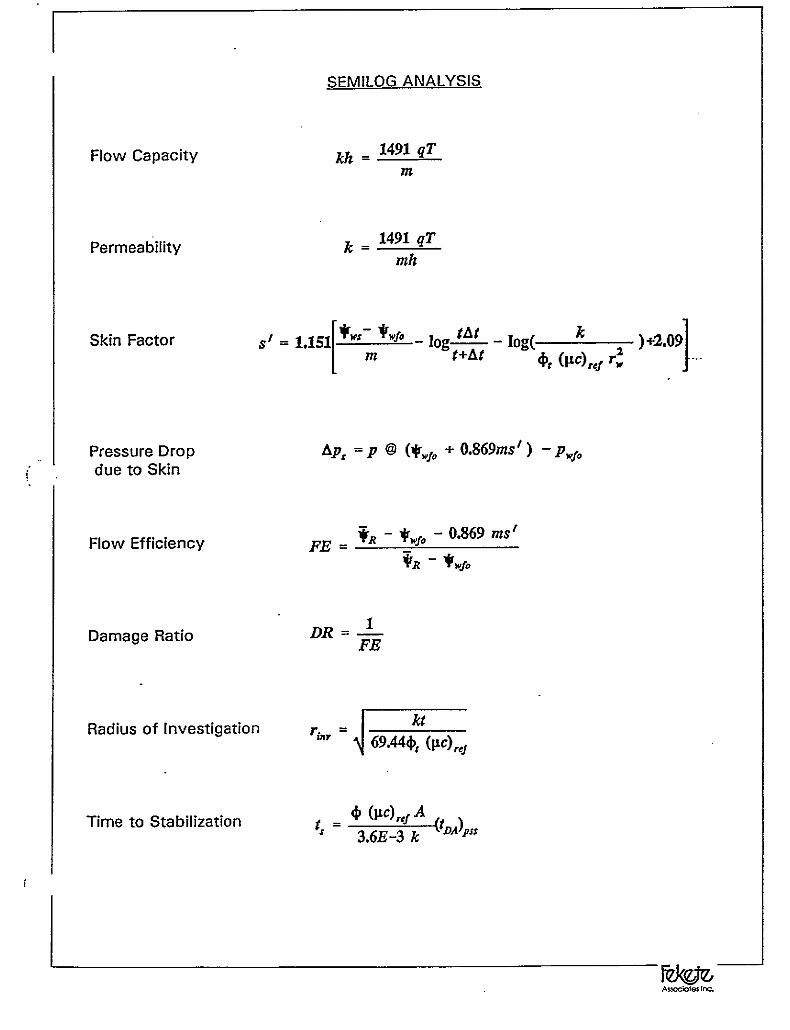
pta fekete pta course (mattar 2004)
DESCRIPTION
Well testTRANSCRIPT
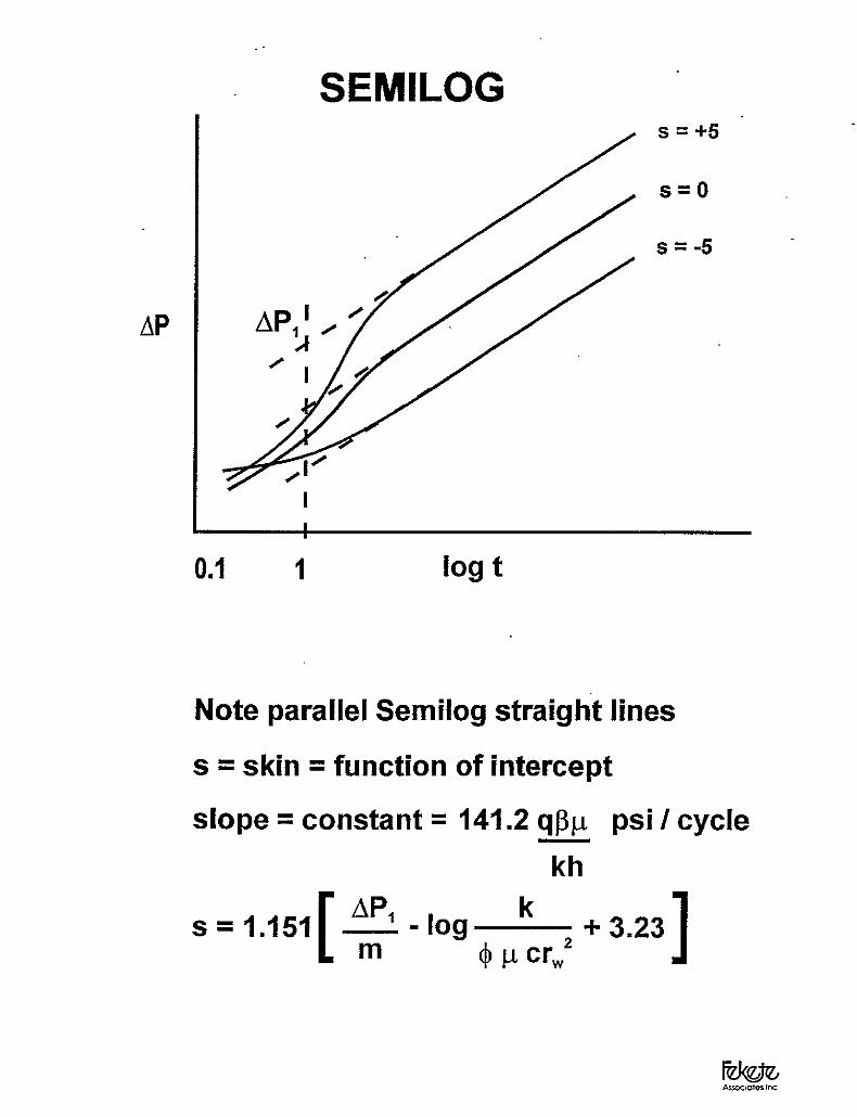
WELL TEST INTERPRETATION
Instructor: Louis Mattar, B.Sc., M.Sc., P.Eng

Course Outline
WELL TEST INTERPRETATION
This course is intended for engineers and specialist who want to learn the reasons forwell testing, and the information that can be derived from it. The procedures andprinciples for analyzing vertical well tests will be extended to apply to horizontal wells.The course will deal with both oil and gas well test interpretation, drillstem tests, wirelineformation tests and production tests, interference tests, detection of boundaries,estimation of stabilized flow rates from short tests, etc.
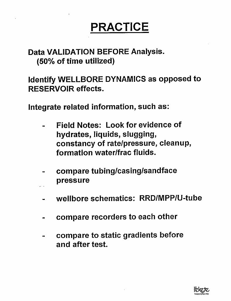
The Practice of well test interpretation will be emphasized over the Theory. To this end,Data Validation and the PPD (Primary Pressure Derivative) will be used to illustratewellbore dynamics, and extricate these effects from the apparent reservoir response.Throughout the course, the theme will be:
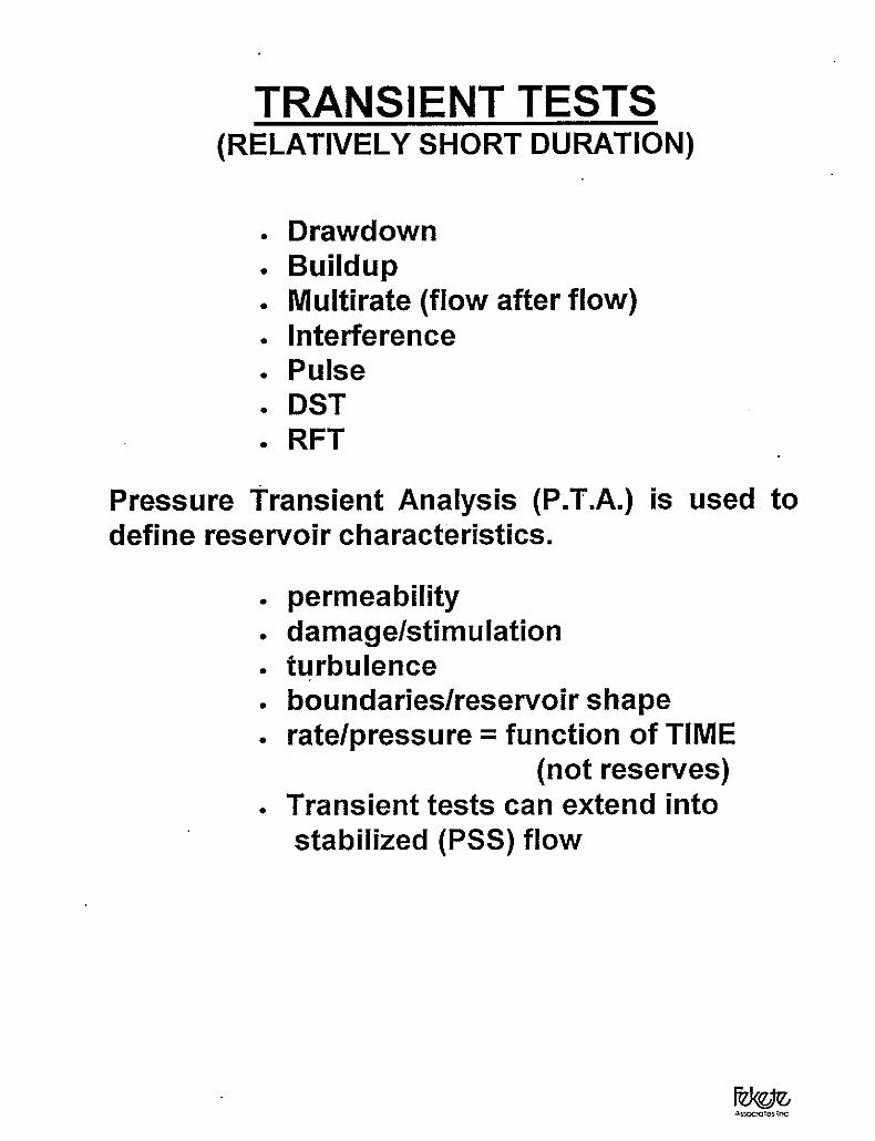
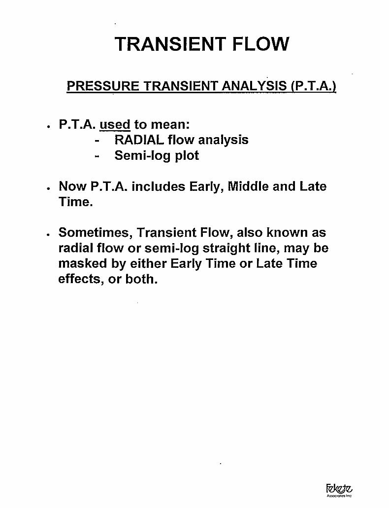
W.T.I >> P.T.A.WELL TEST INTERPRETATION (W.T.I.)
involves a lot more than simplyPRESSURE TRANSIENT ANALYSIS (P.T.A.)
This course is aimed at obtaining an understanding of the concepts. These will bepresented graphically (using a computer), thus keeping equations to a minimum. ThePractical aspects of the interpretation process will be highlighted.
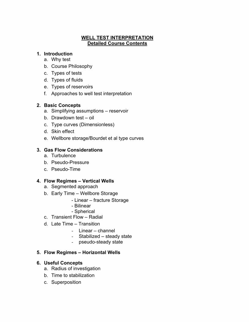
WELL TEST INTERPRETATIONDetailed Course Contents
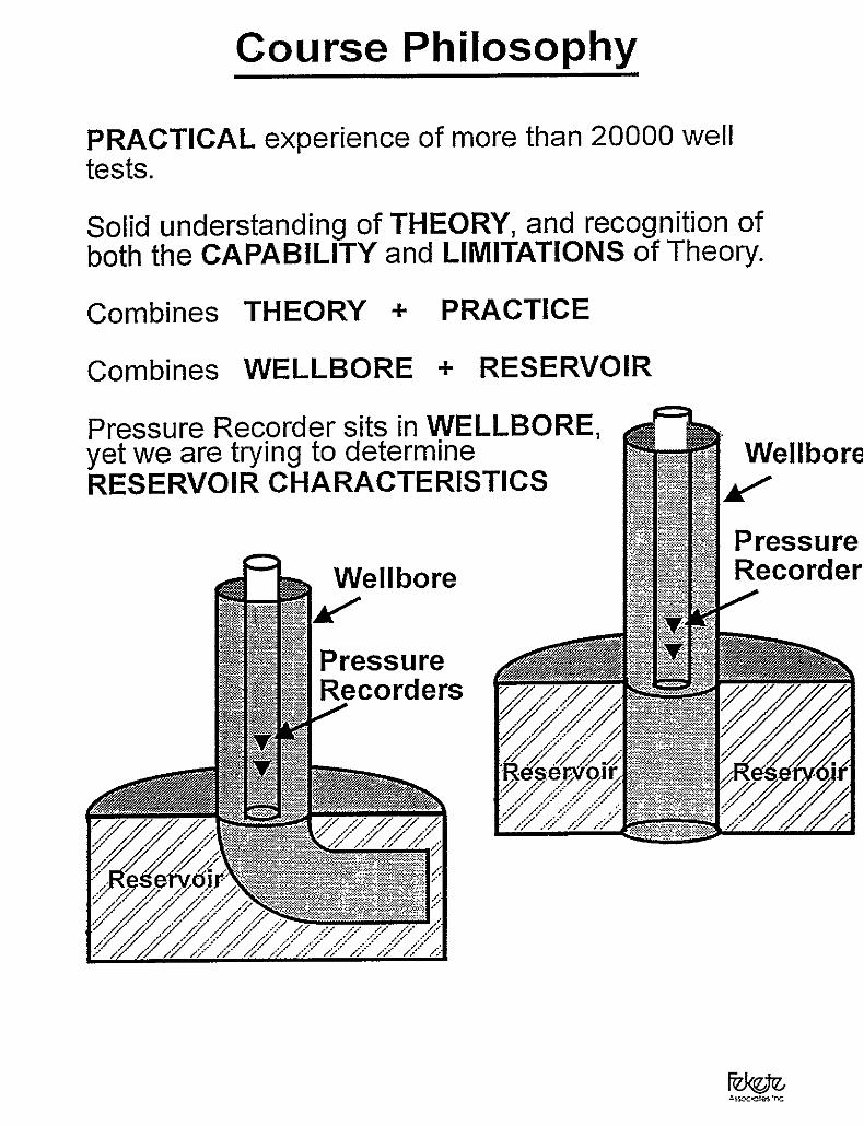
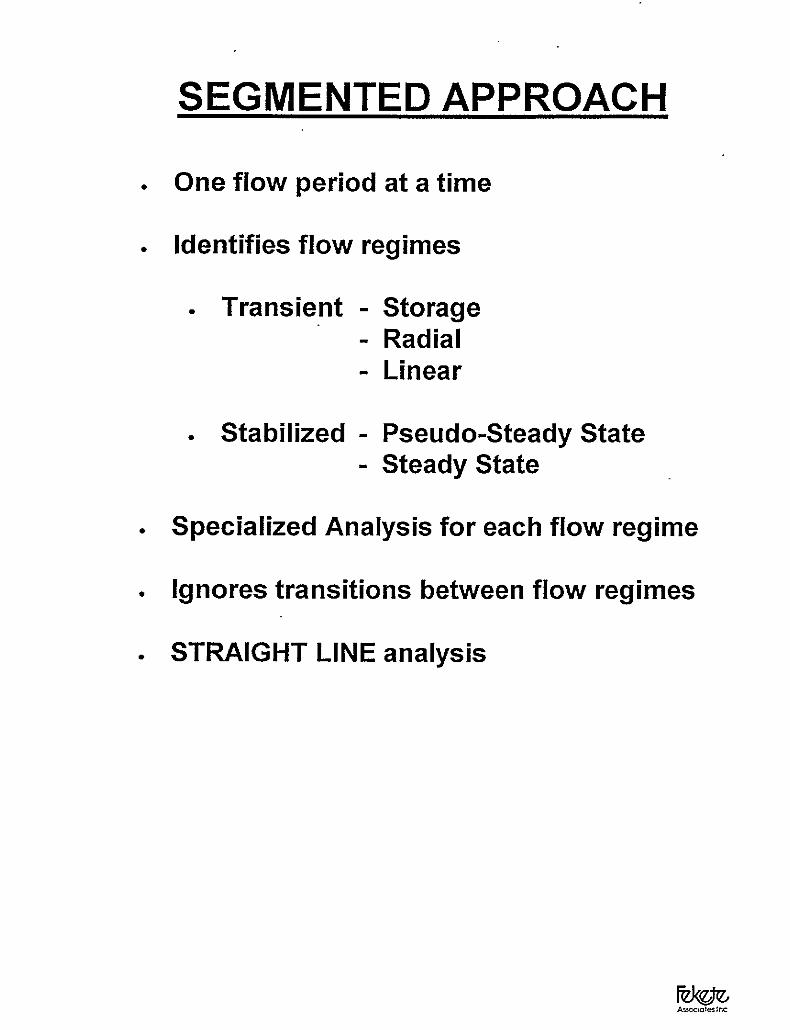
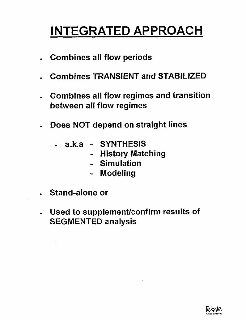
1. Introductiona. Why testb. Course Philosophyc. Types of testsd. Types of fluidse. Types of reservoirsf. Approaches to well test interpretation
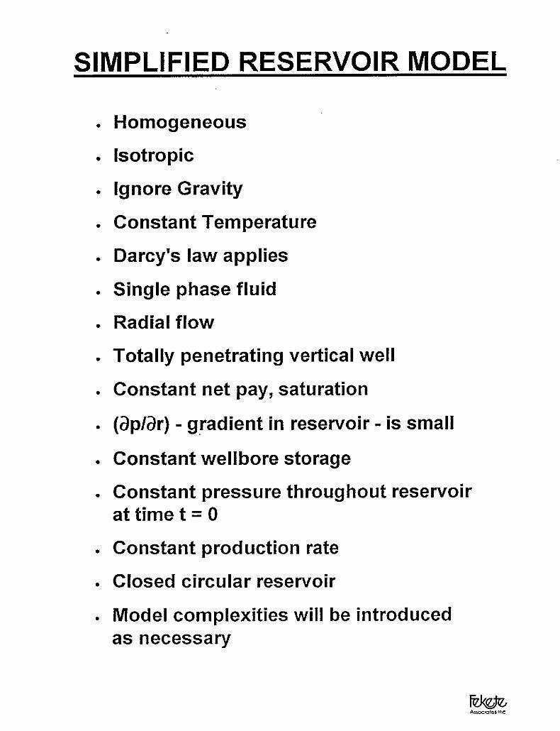
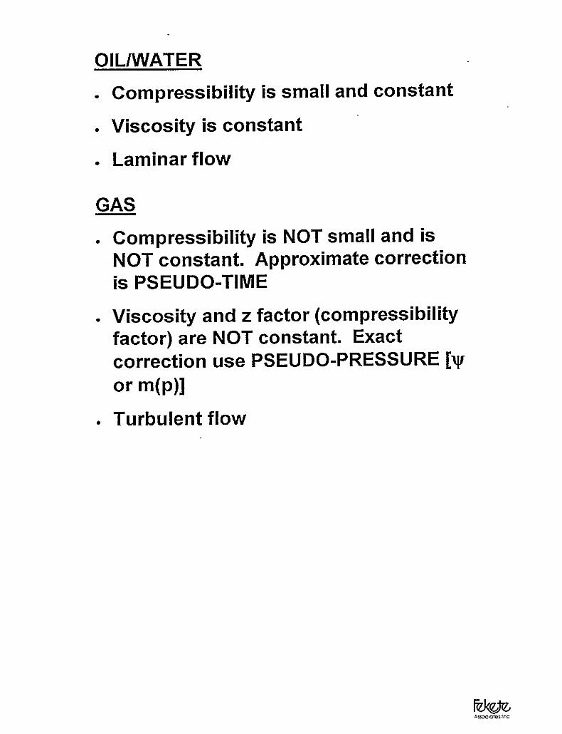
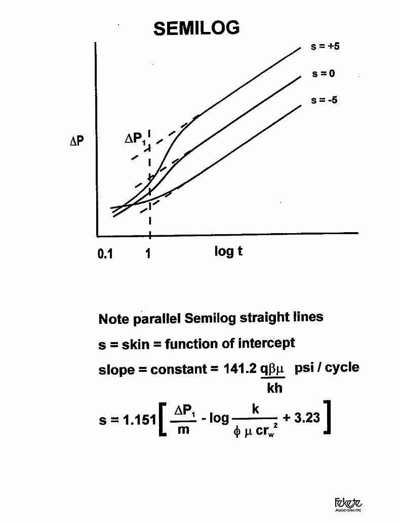
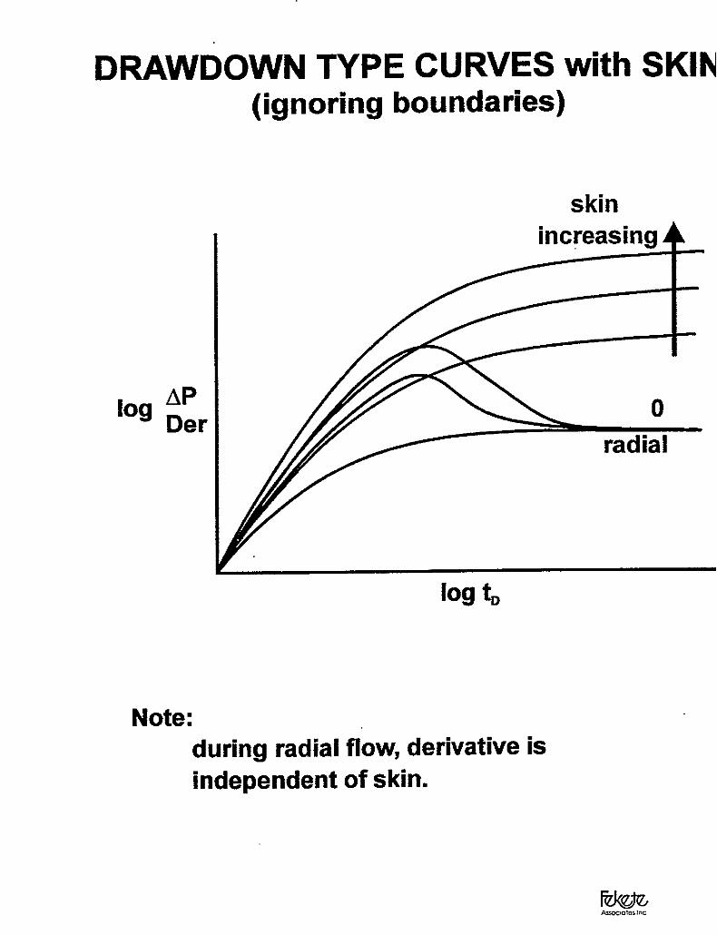
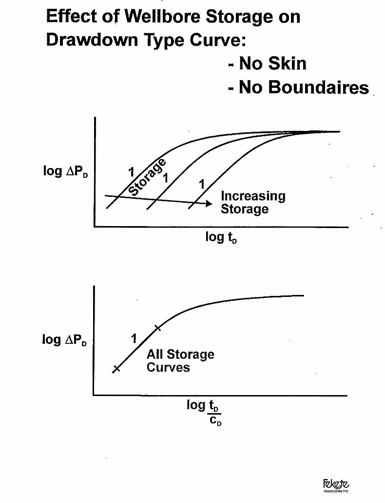
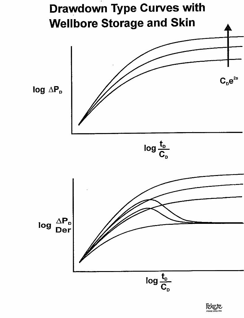
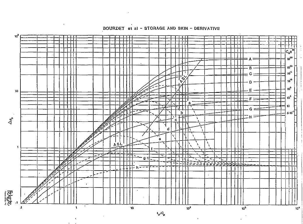
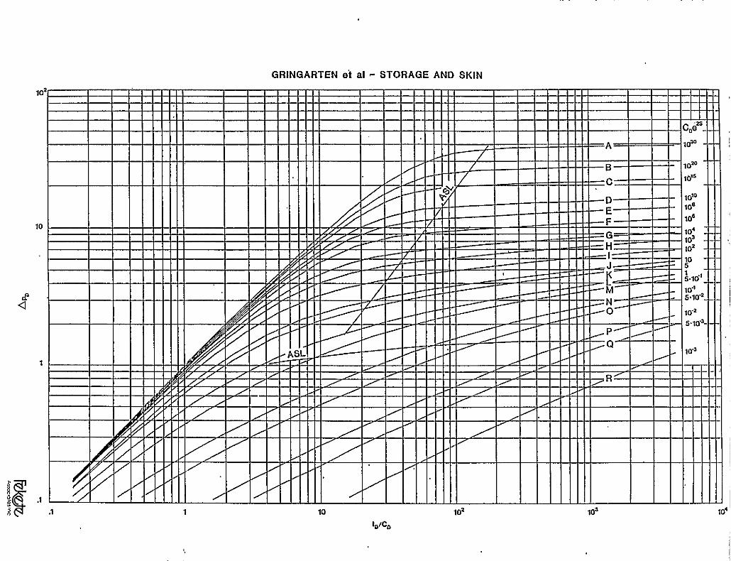
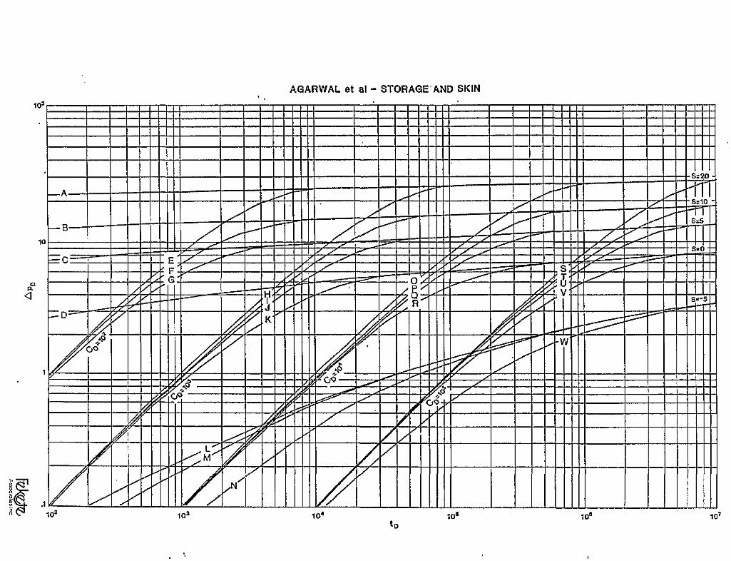
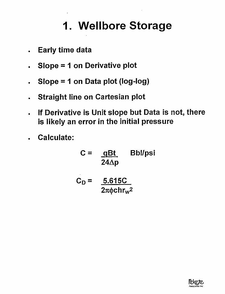
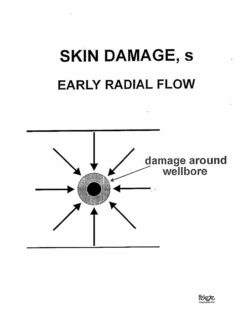
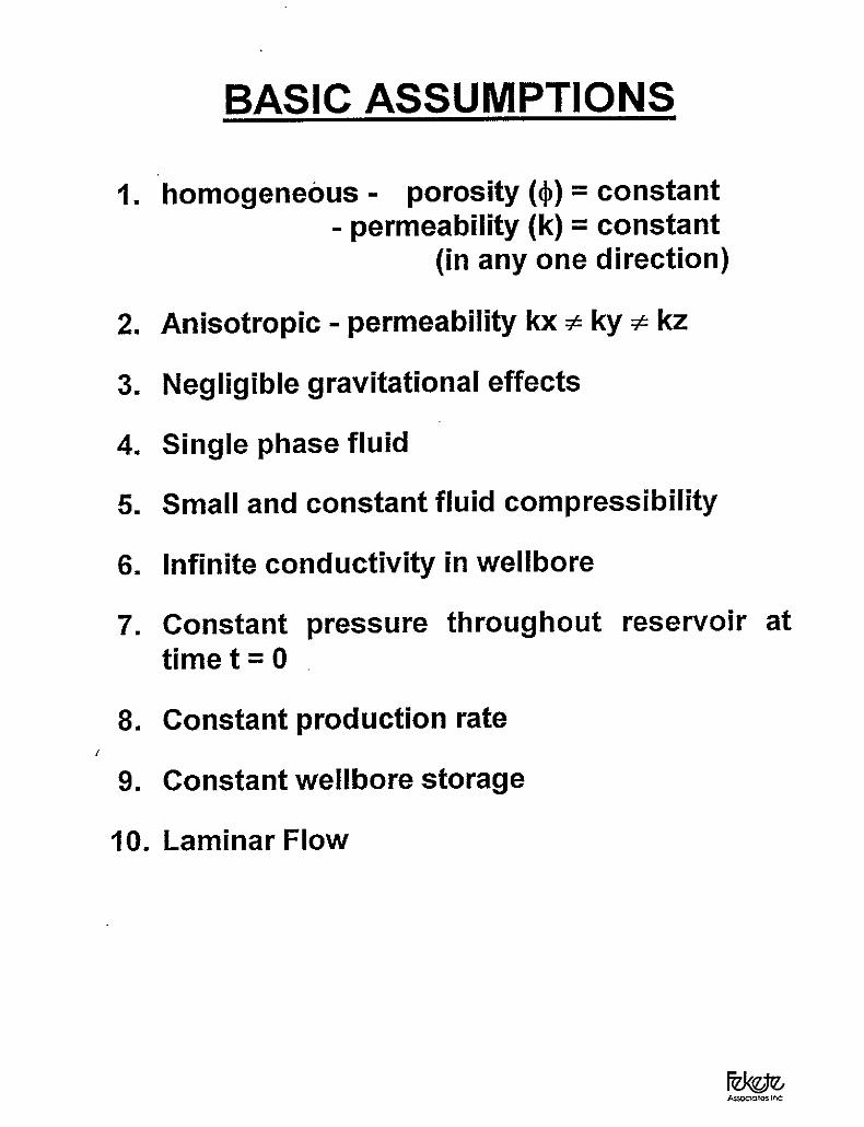
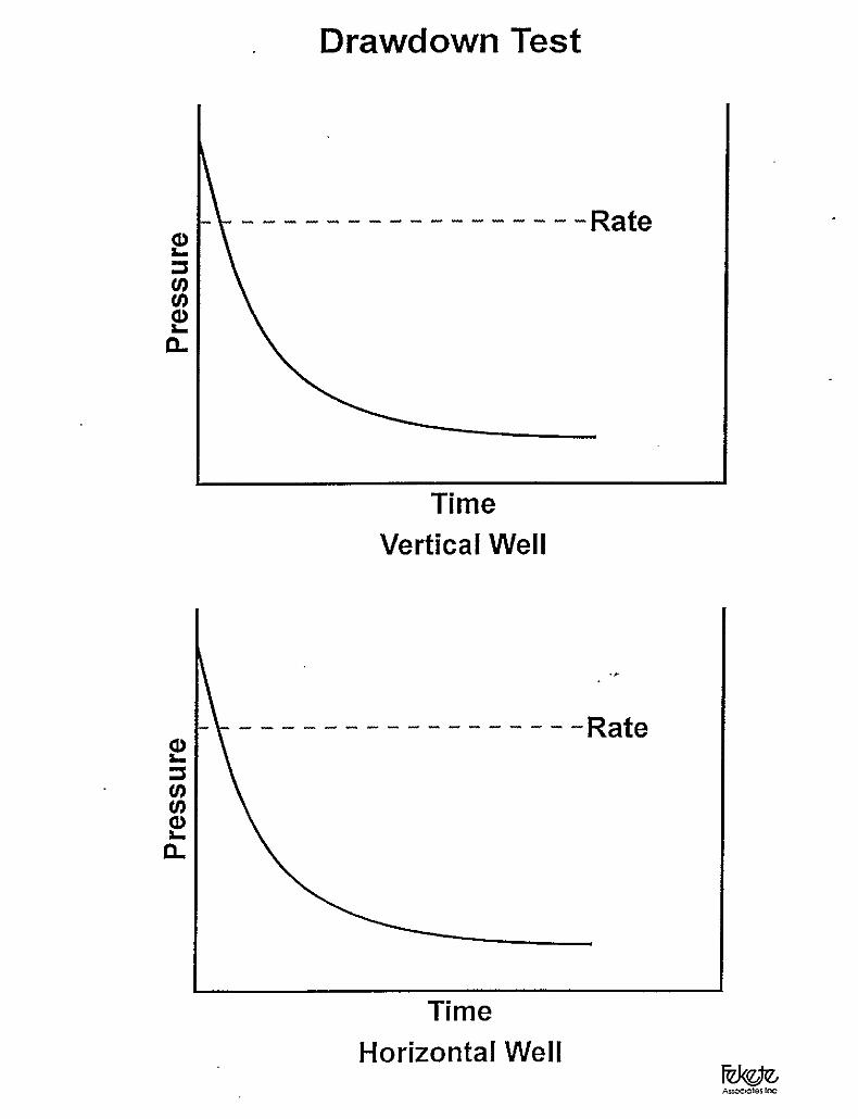
2. Basic Conceptsa. Simplifying assumptions – reservoirb. Drawdown test – oilc. Type curves (Dimensionless)d. Skin effecte. Wellbore storage/Bourdet et al type curves
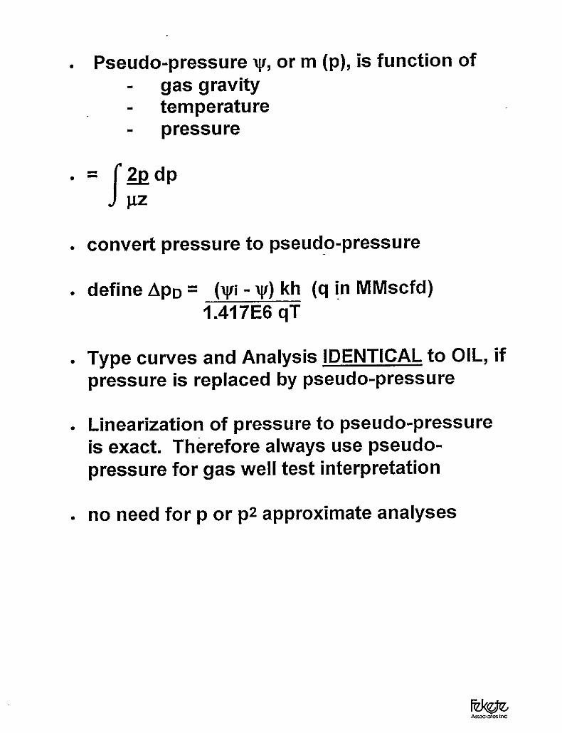
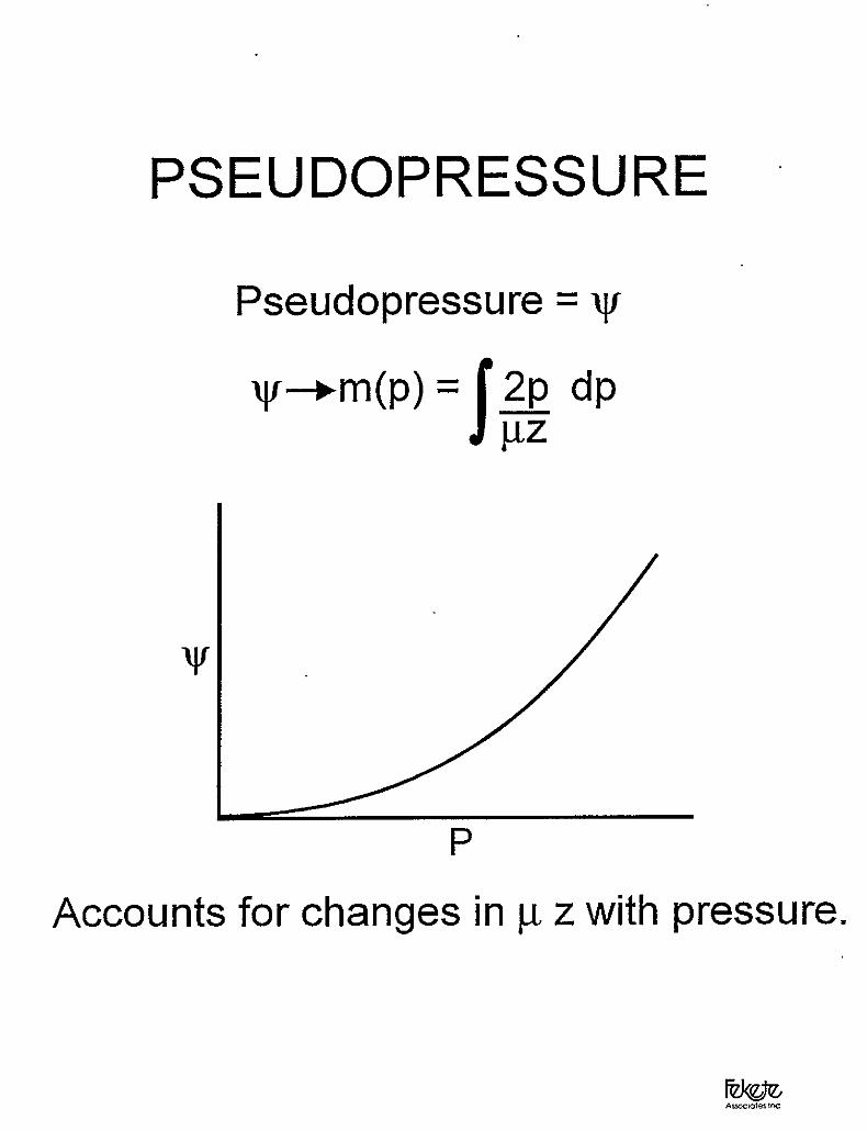
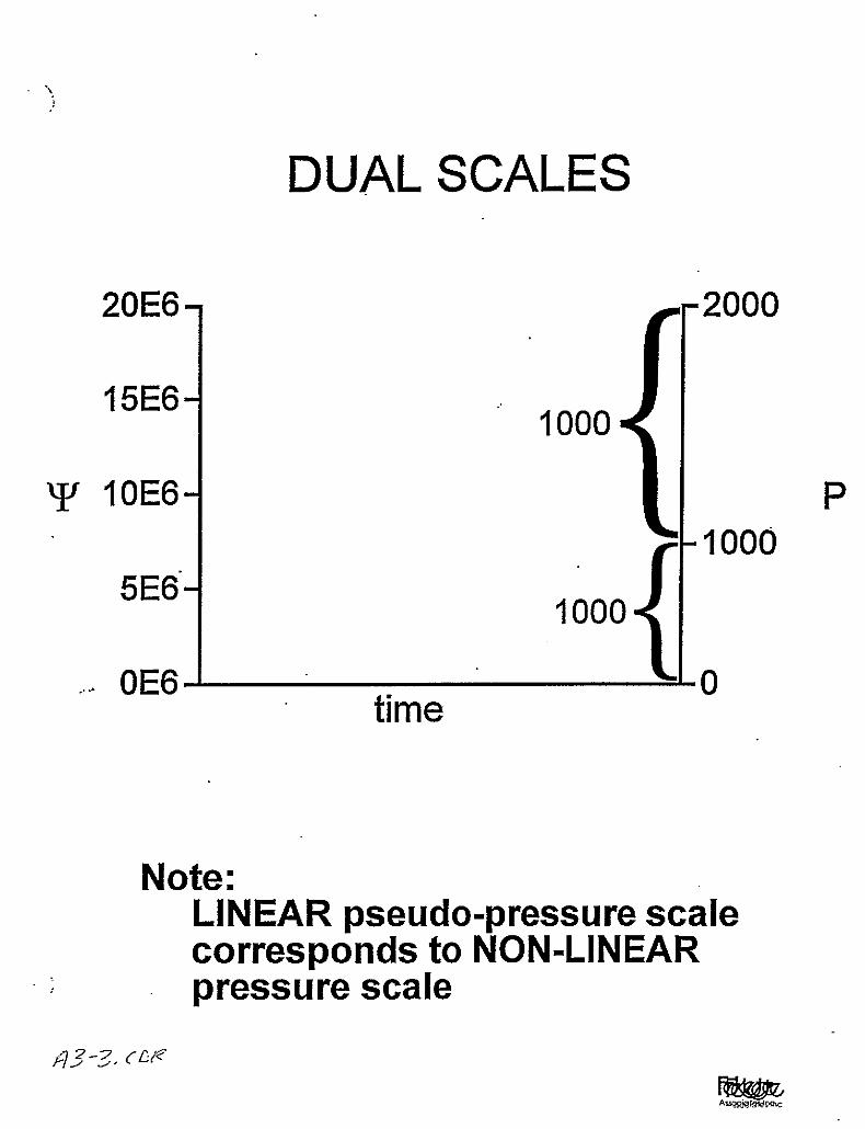
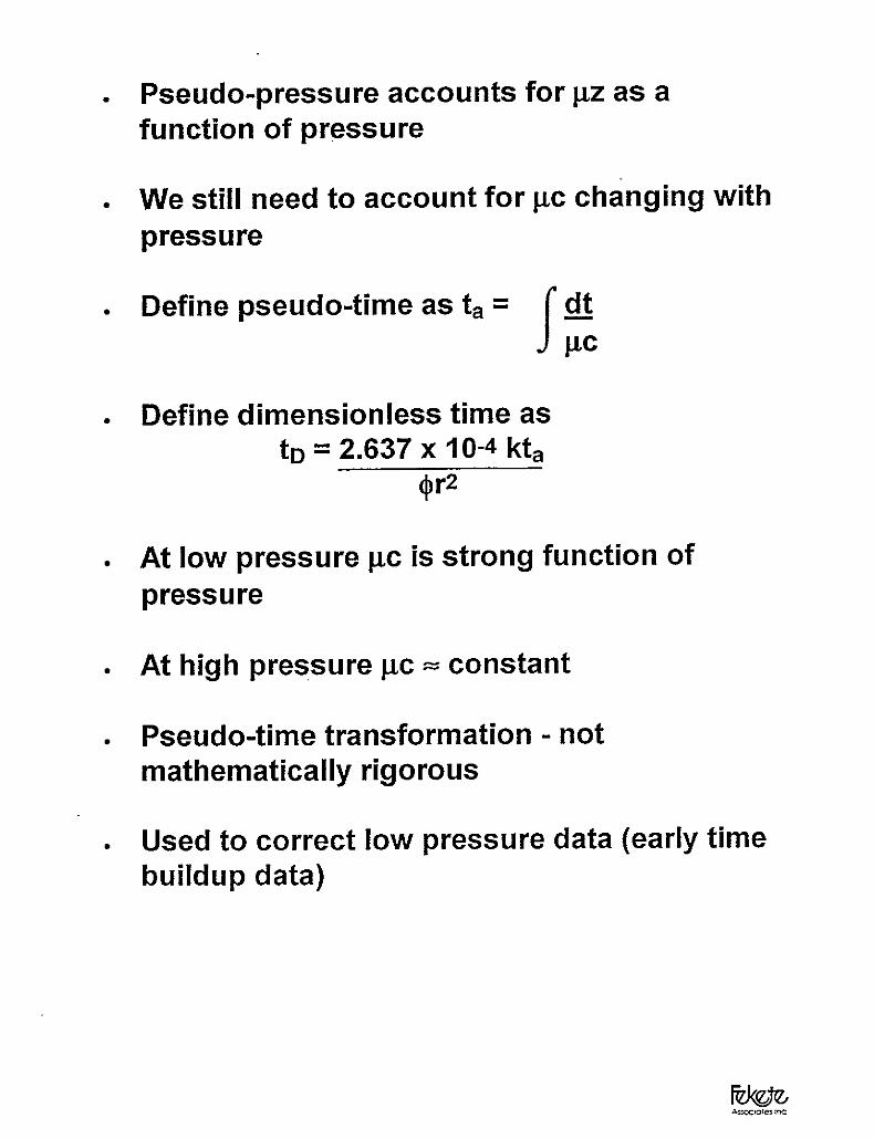
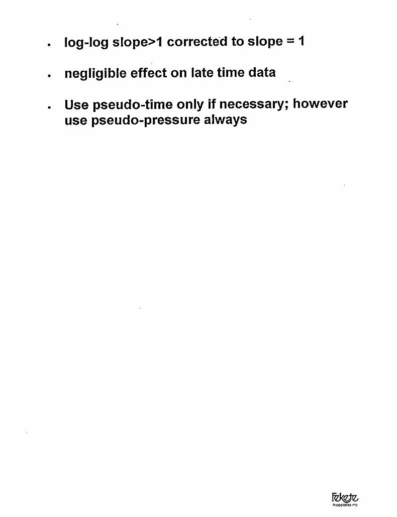
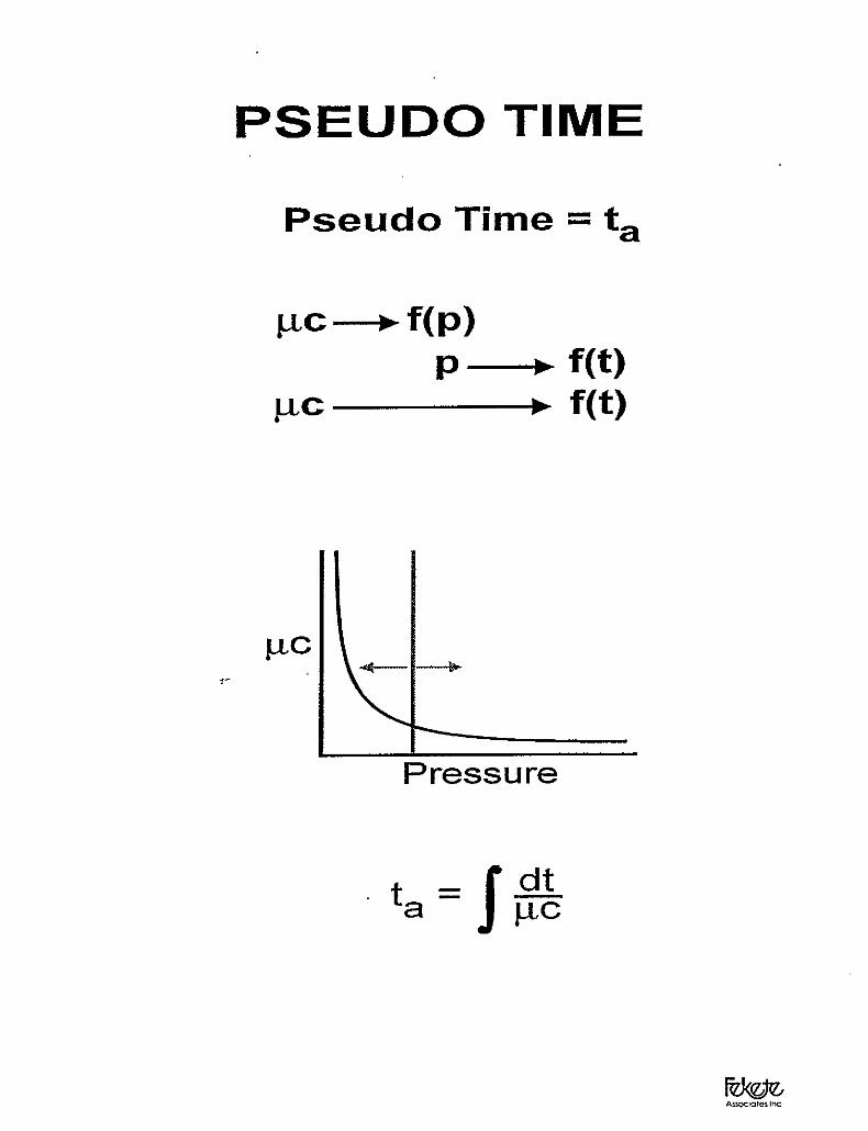
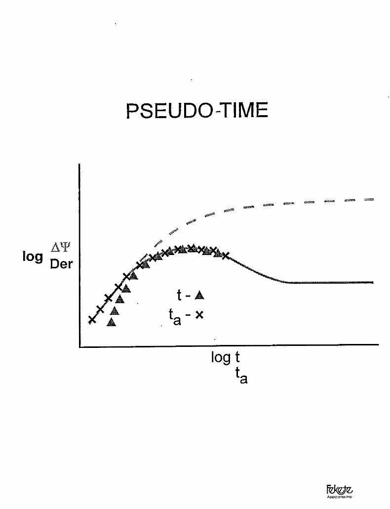
3. Gas Flow Considerationsa. Turbulenceb. Pseudo-Pressurec. Pseudo-Time
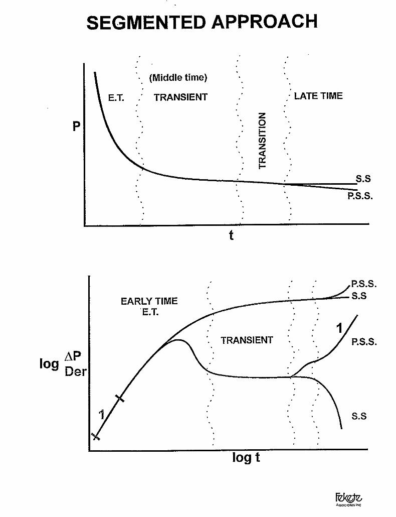
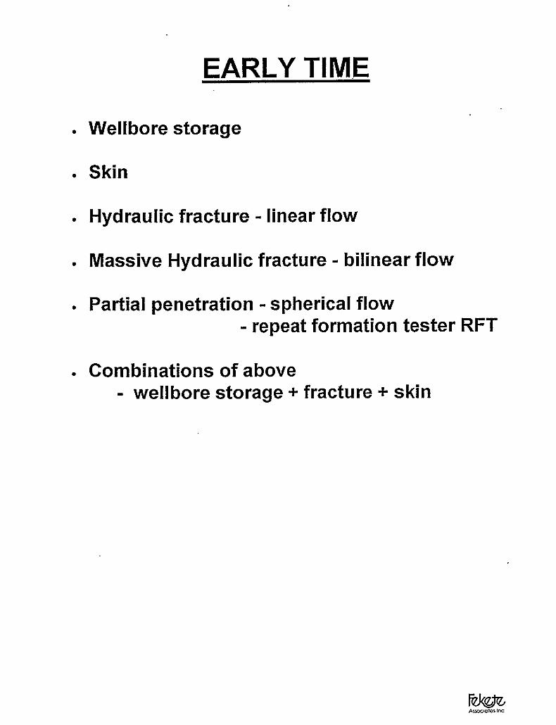
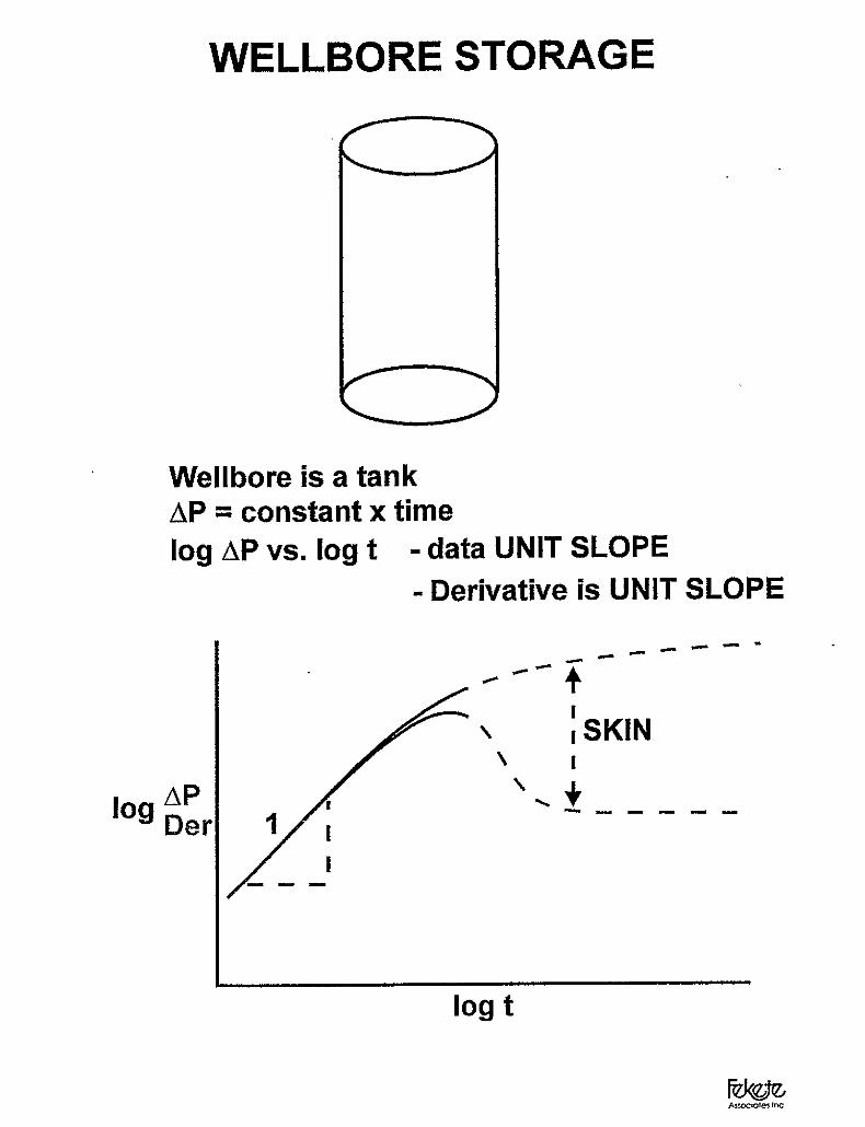
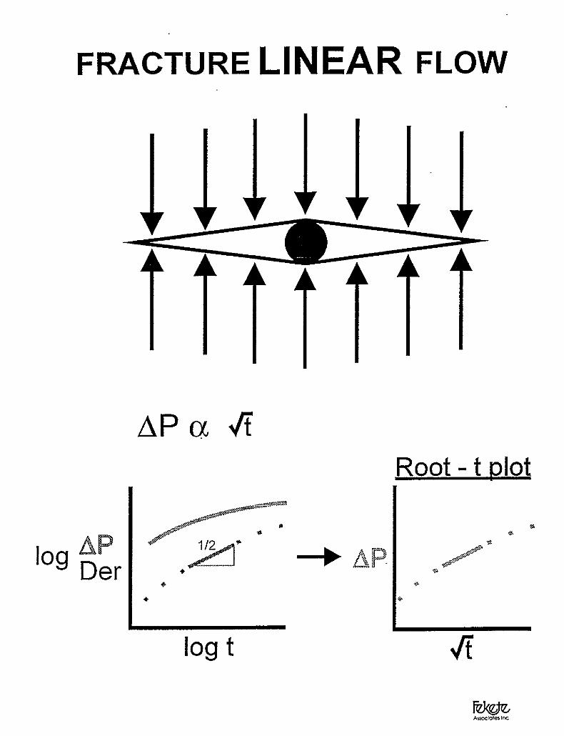
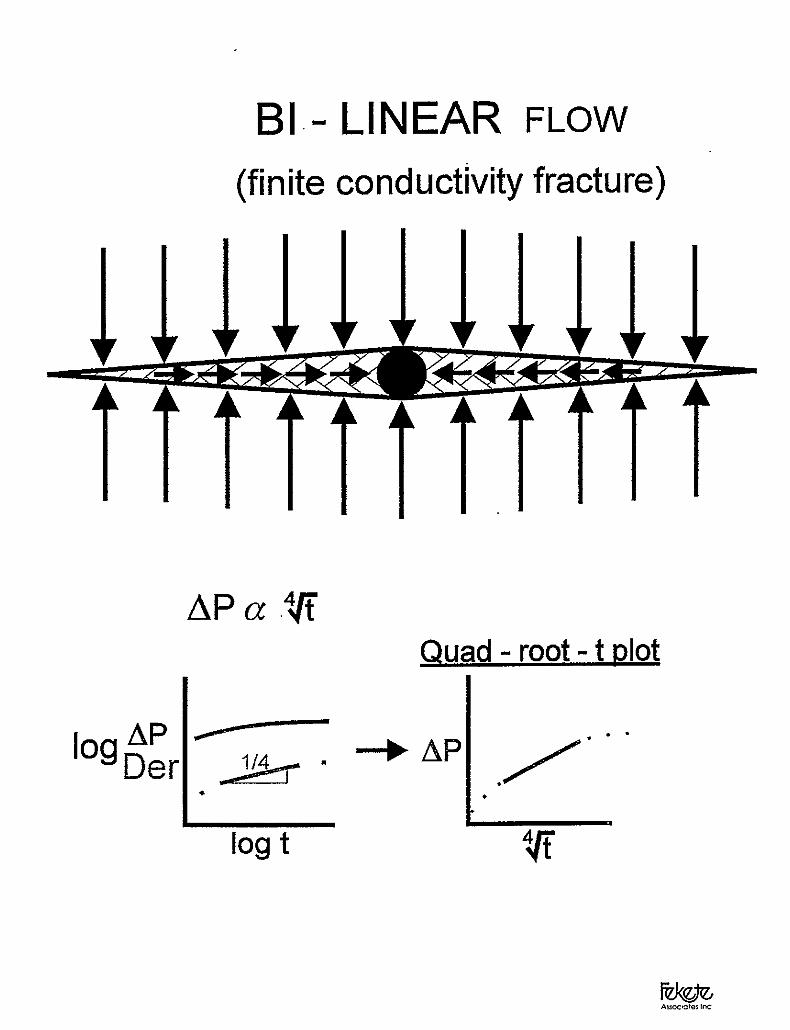
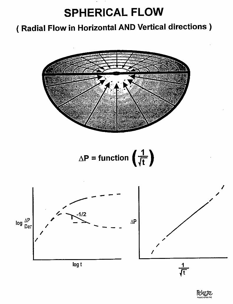
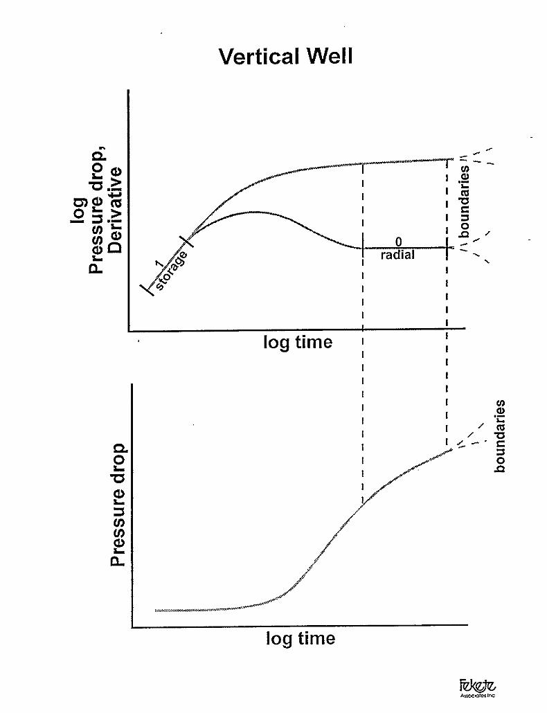
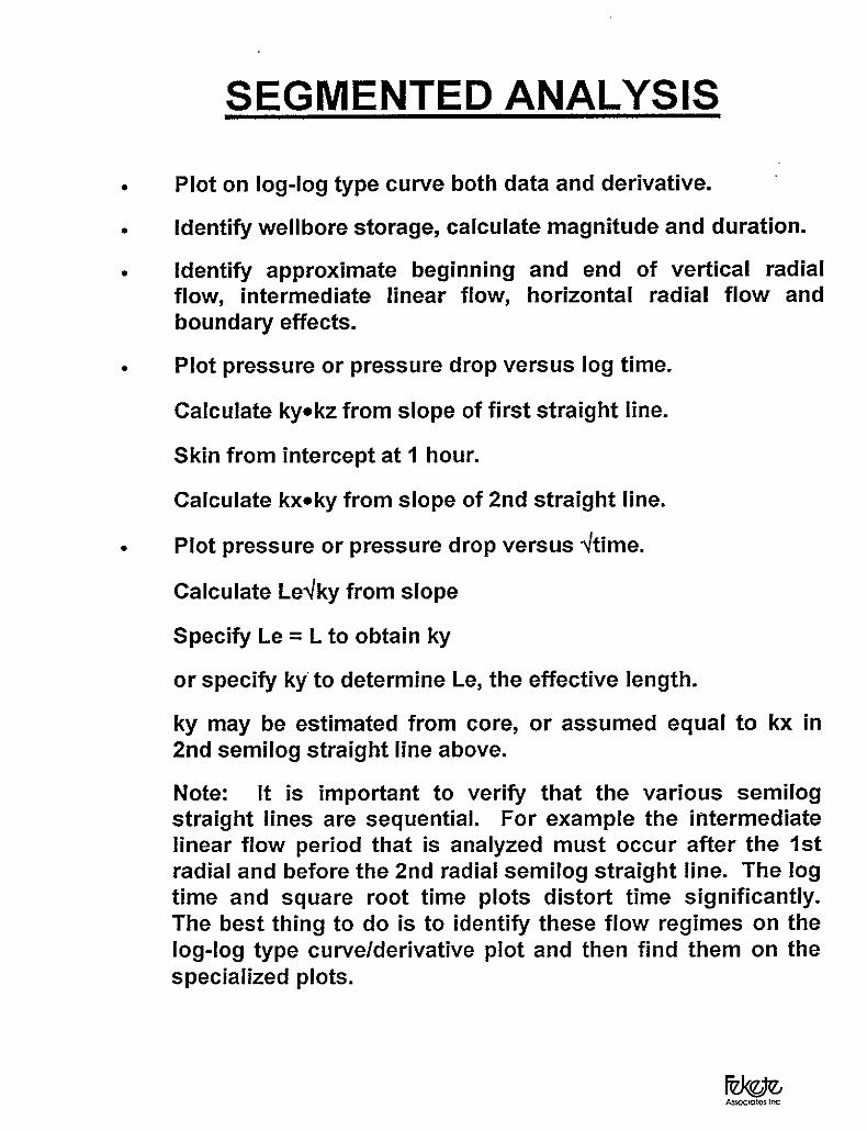
4. Flow Regimes – Vertical Wellsa. Segmented approachb. Early Time – Wellbore Storage
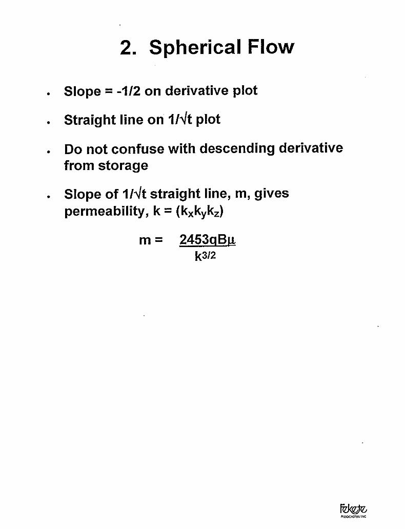
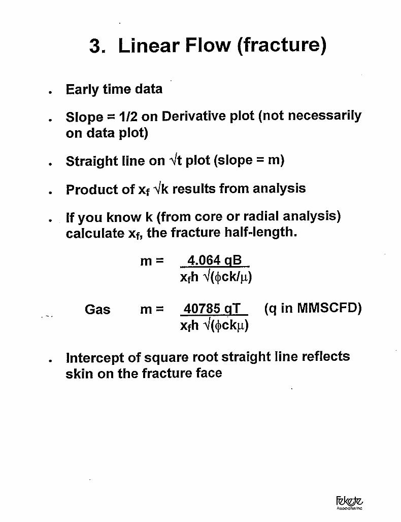
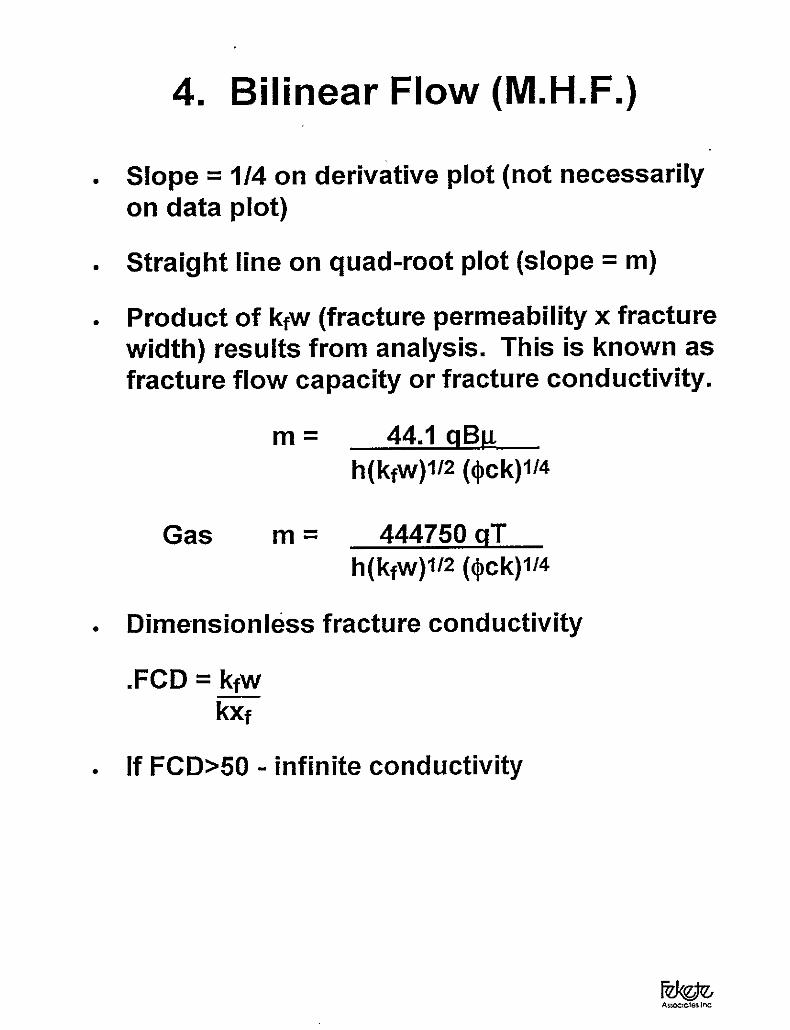
- Linear – fracture Storage- Bilinear- Spherical
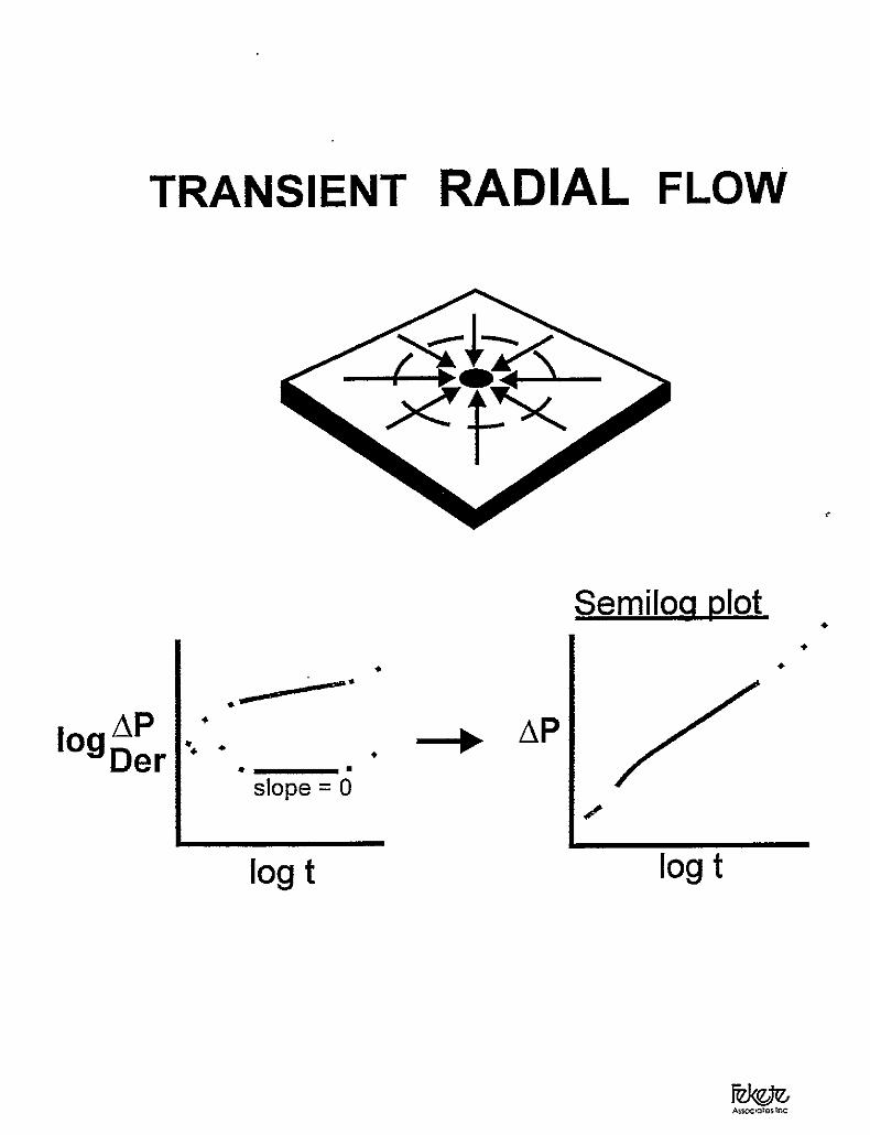
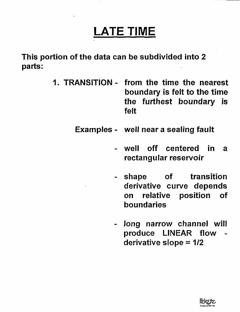
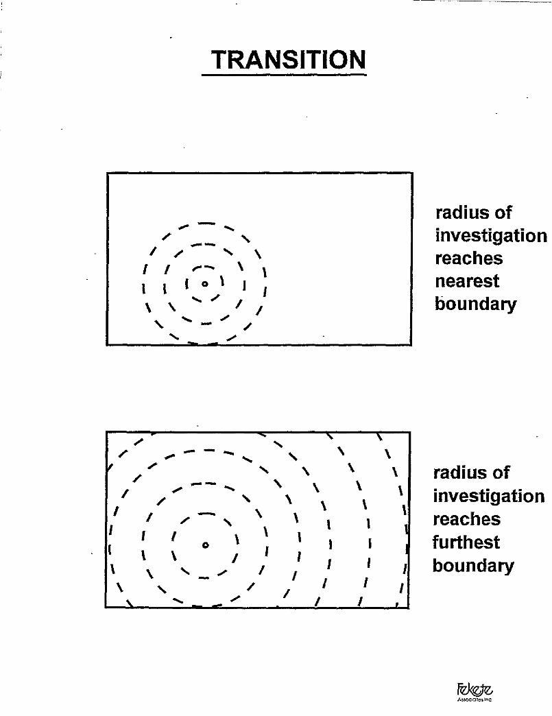
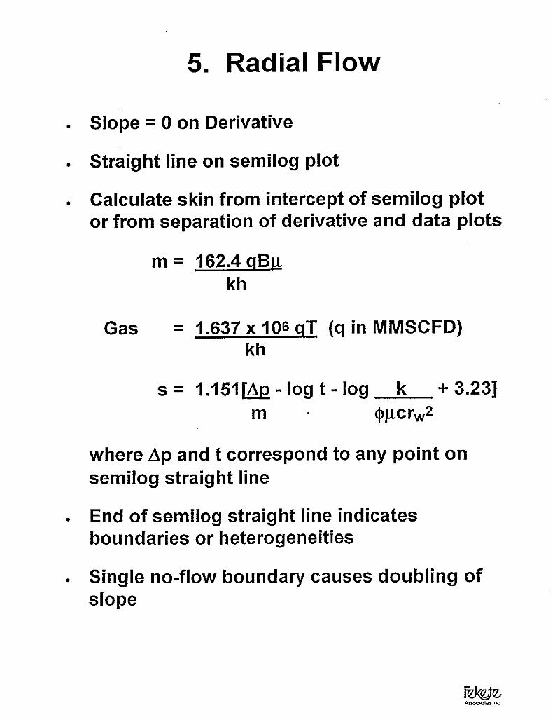
c. Transient Flow – Radiald. Late Time – Transition
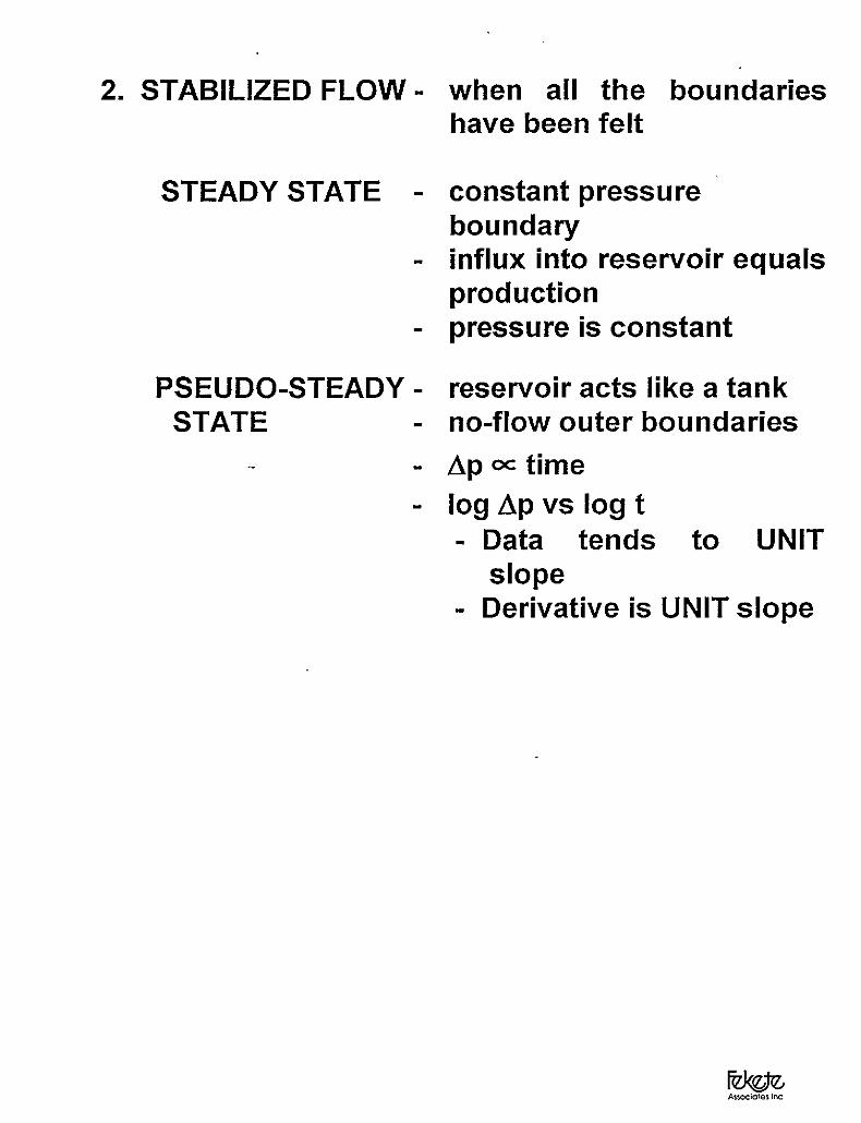
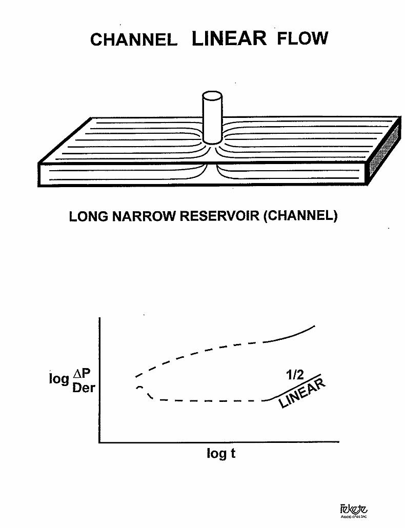
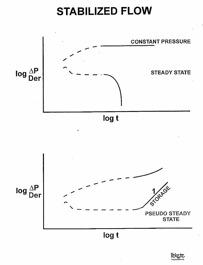
- Linear – channel- Stabilized – steady state- pseudo-steady state
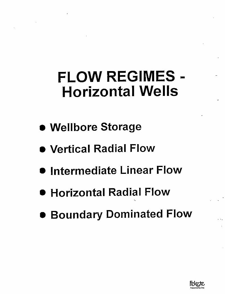
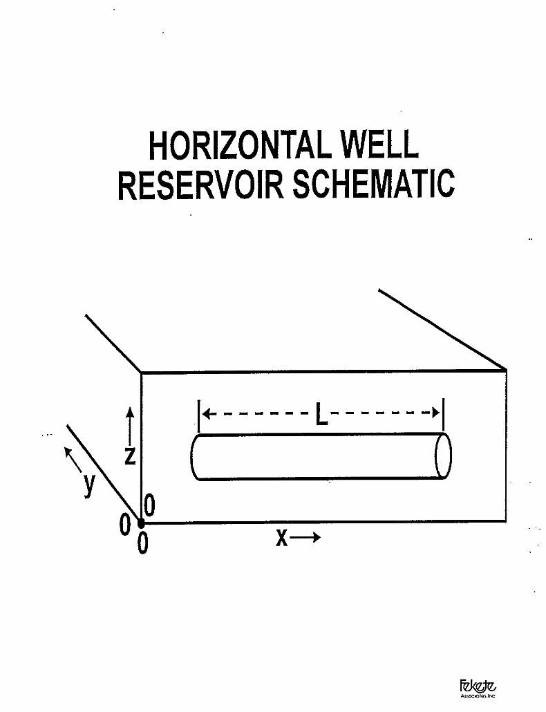
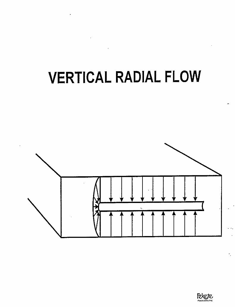
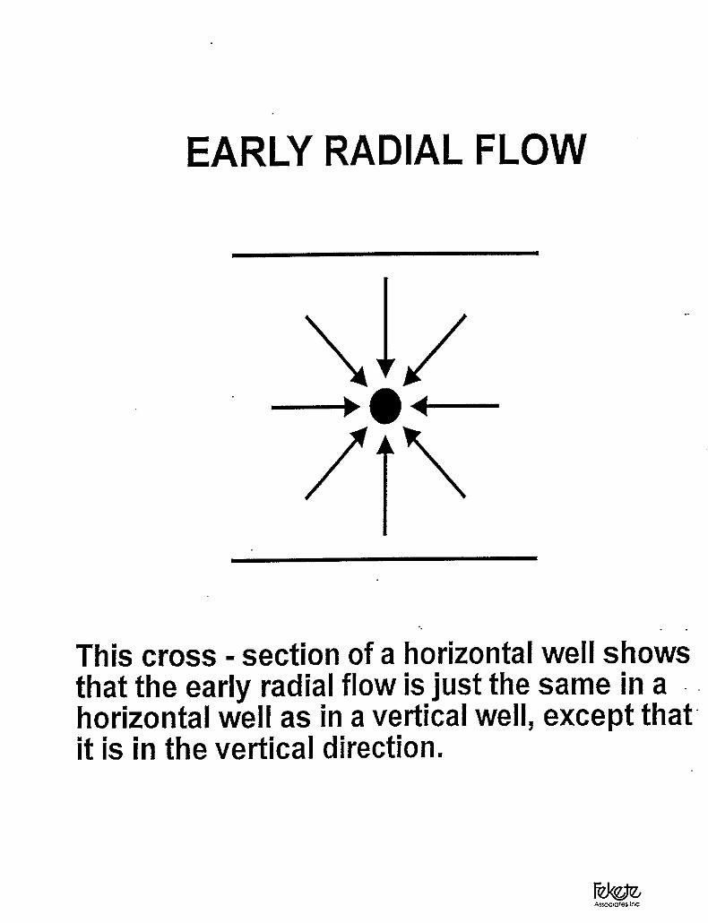
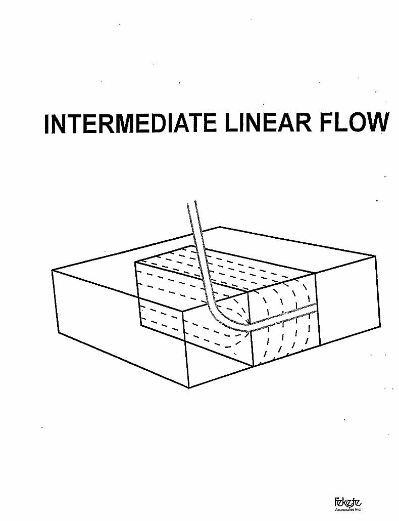
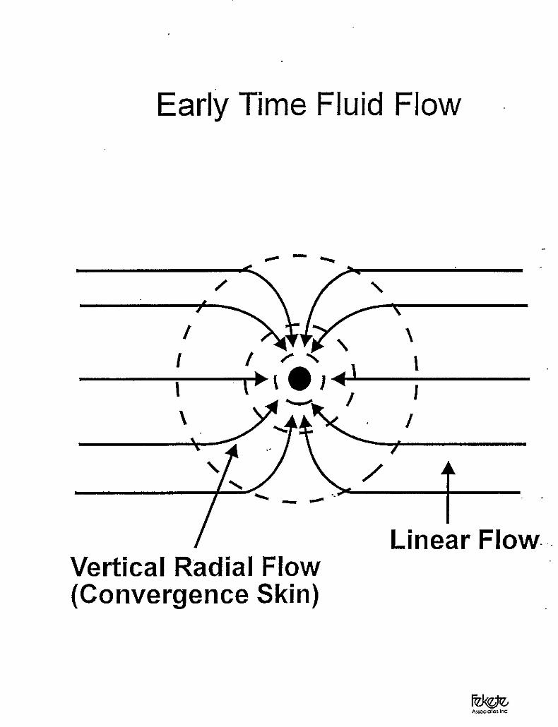
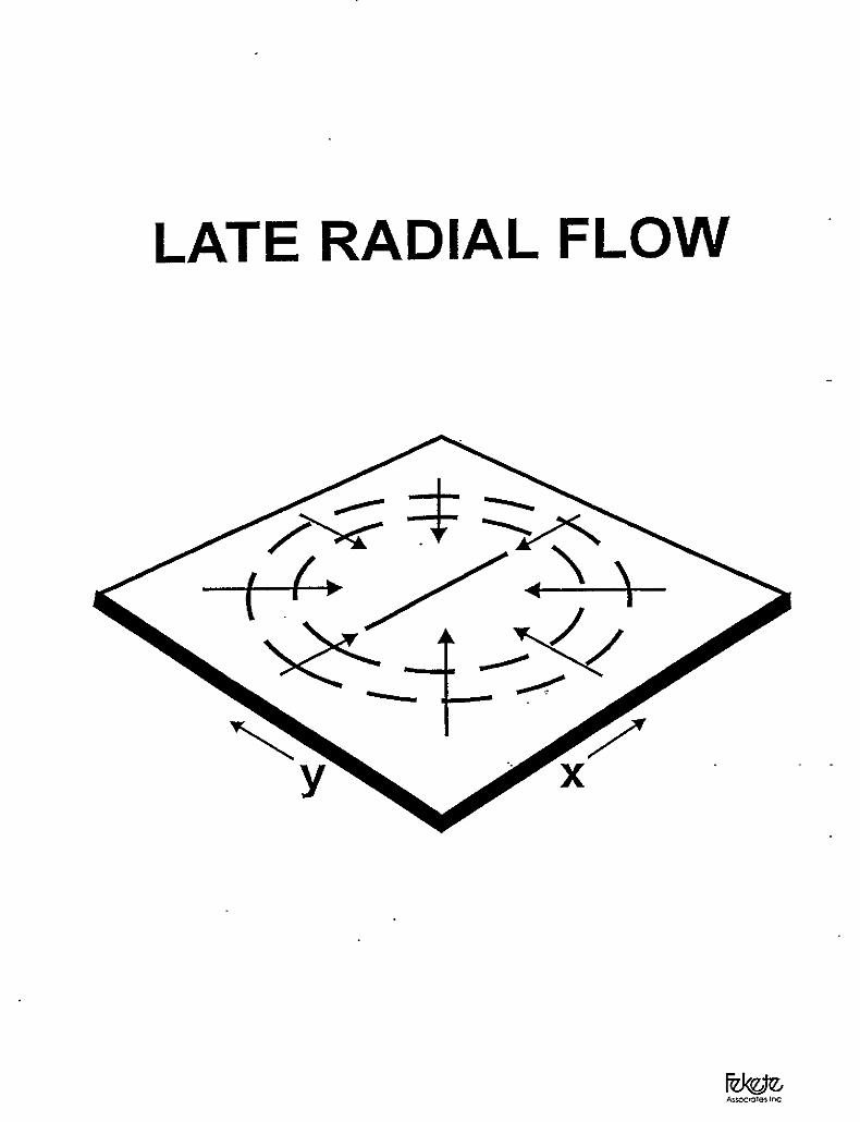
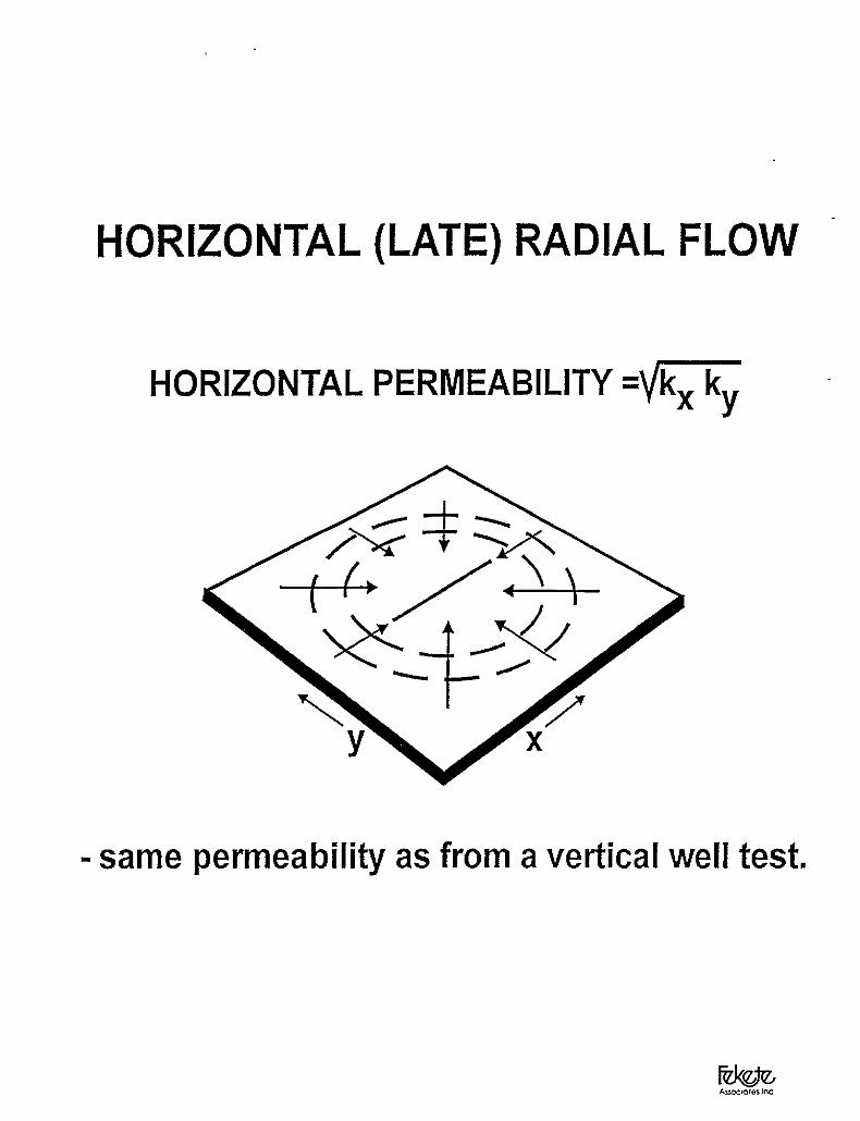
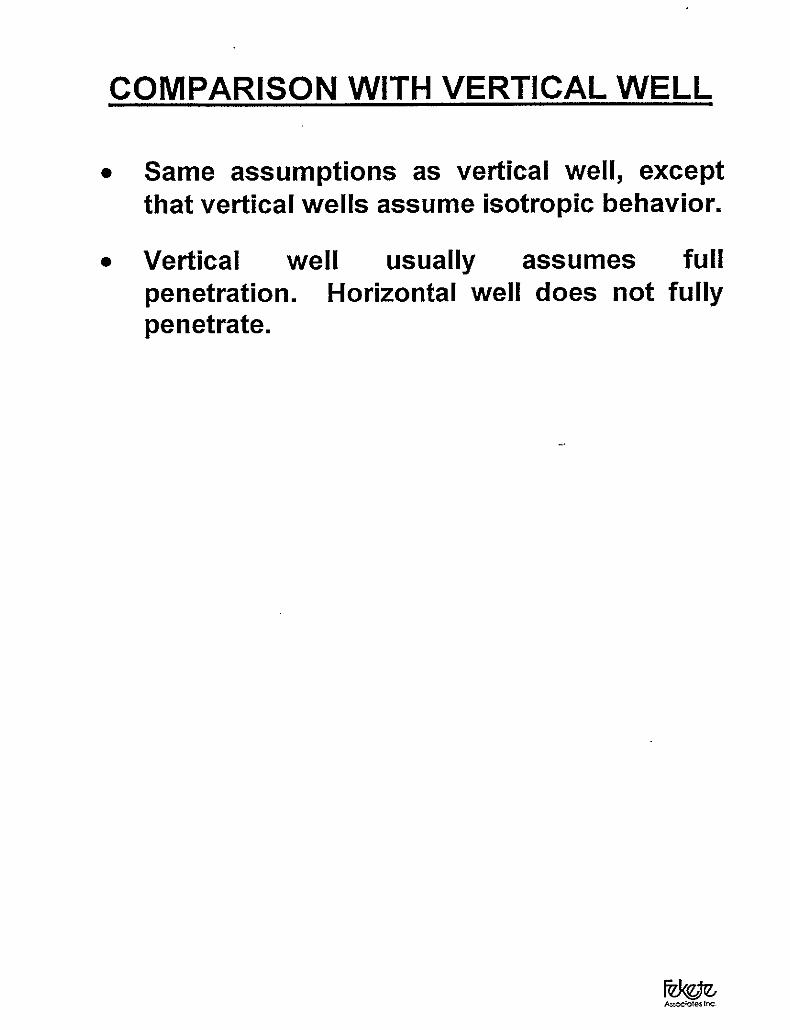
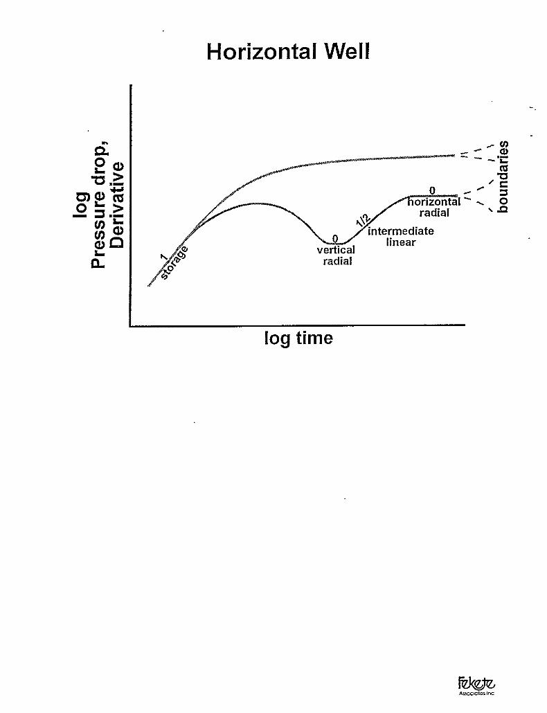
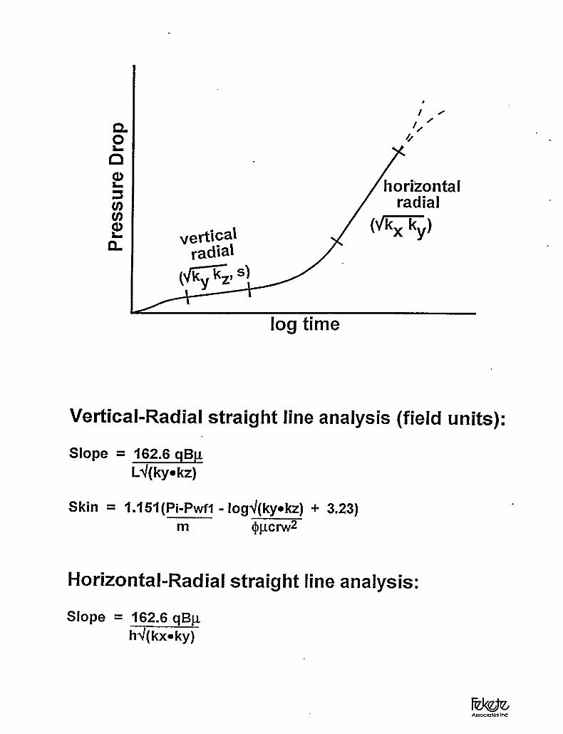
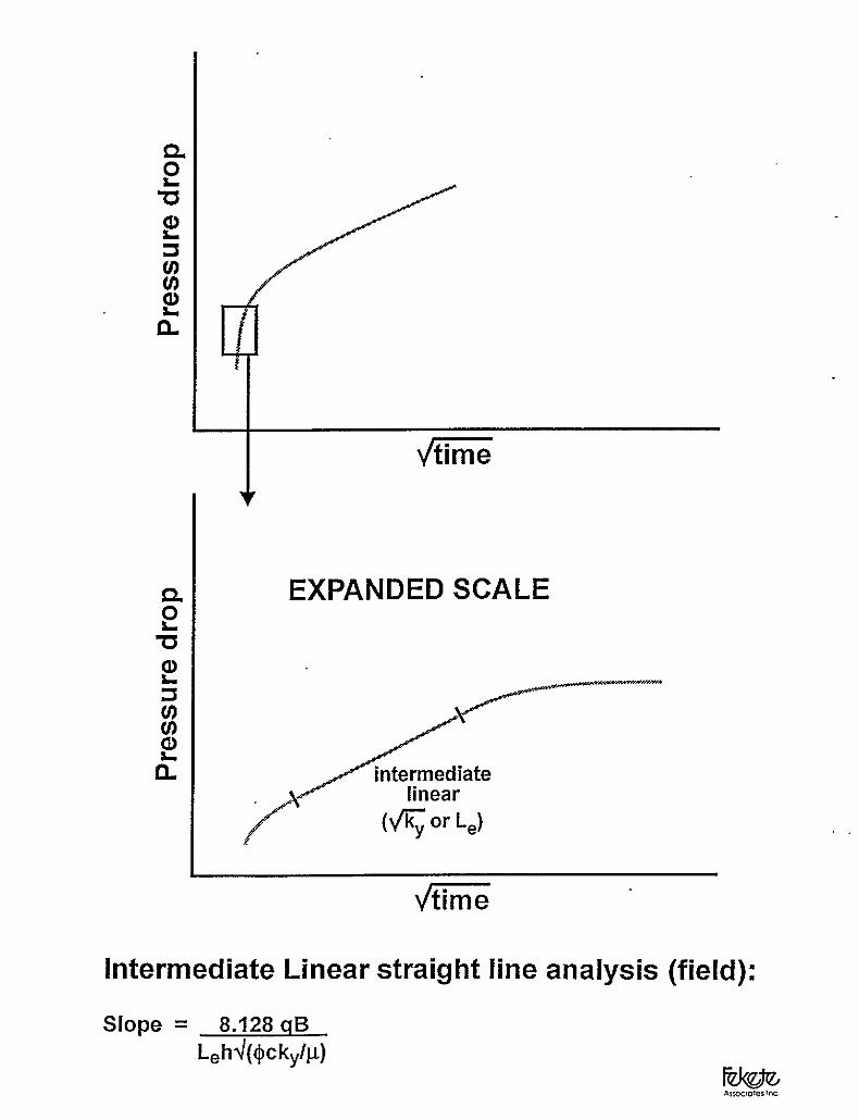
5. Flow Regimes – Horizontal Wells
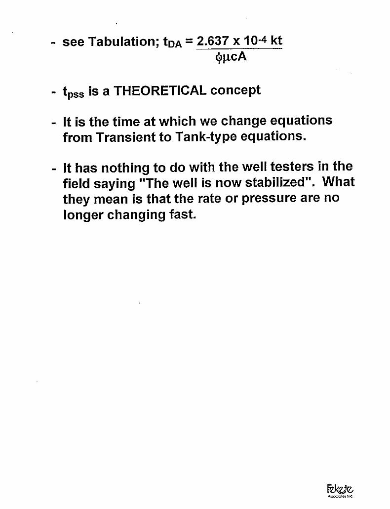
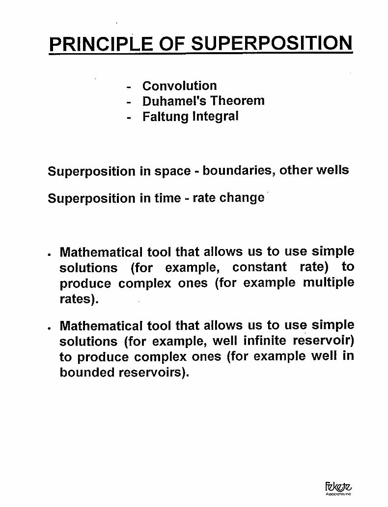
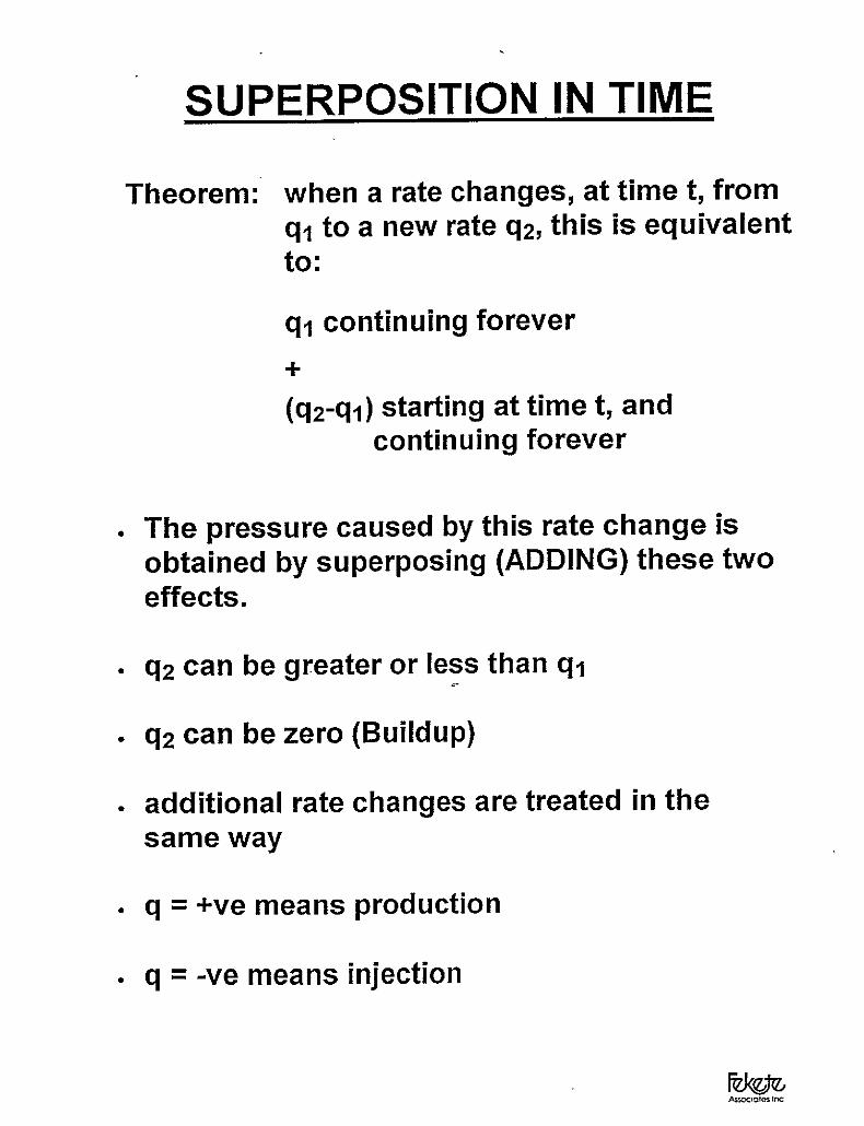
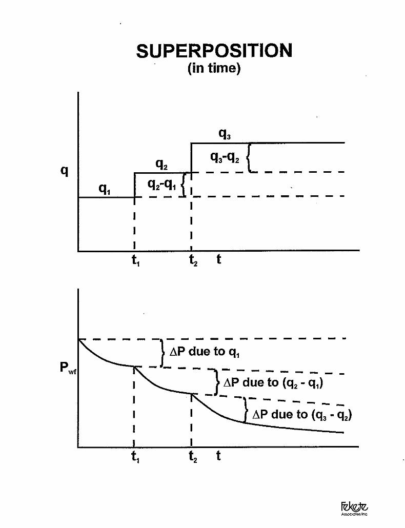
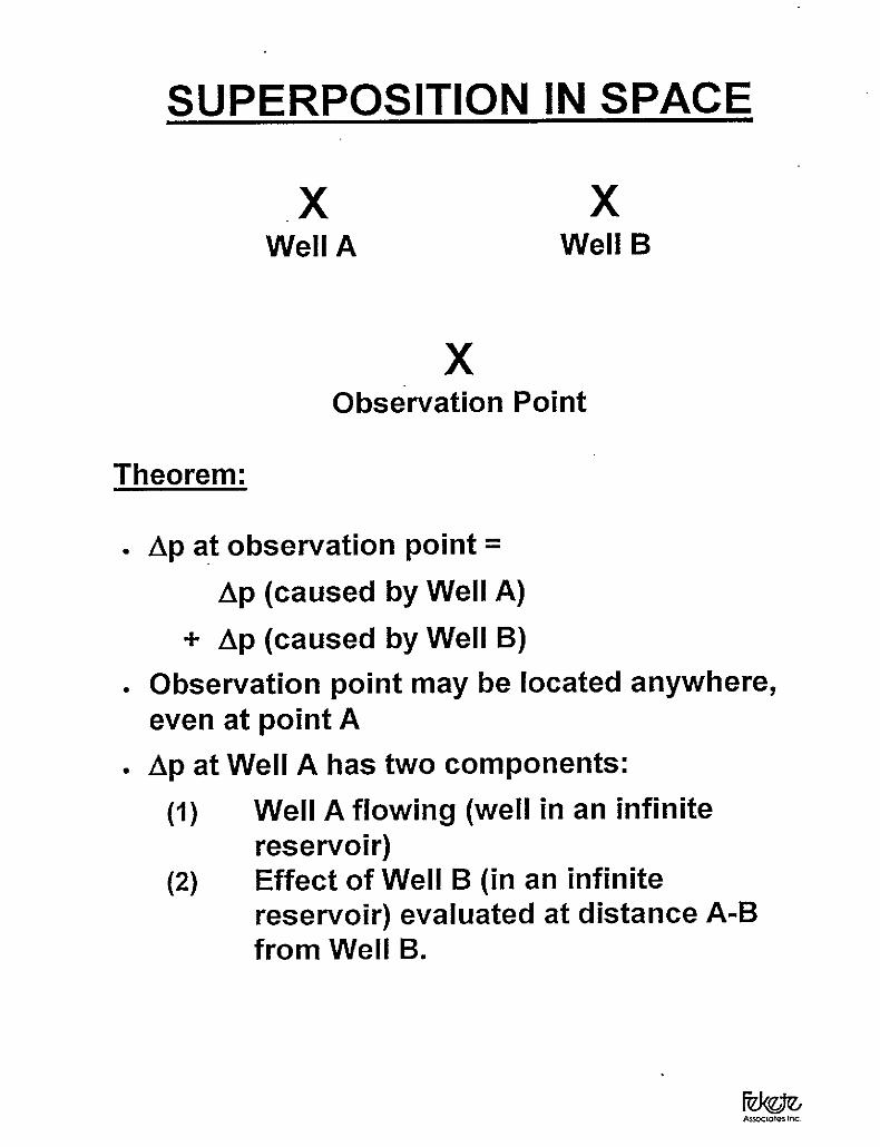
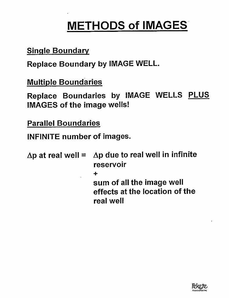
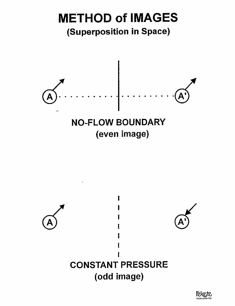
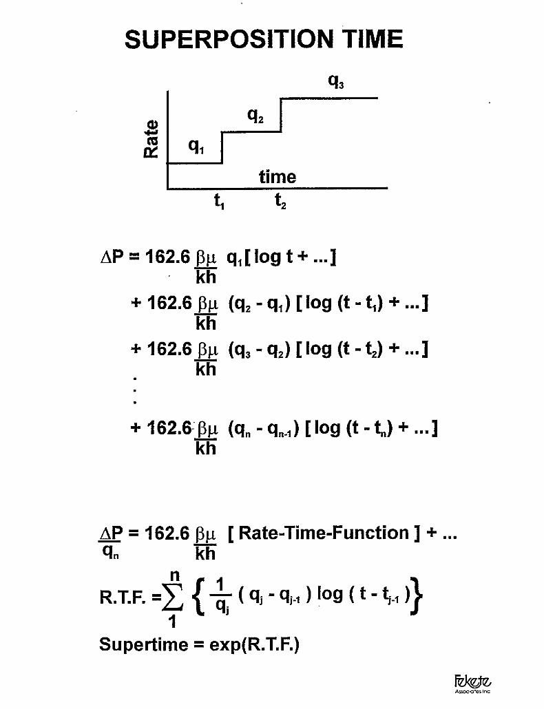
6. Useful Conceptsa. Radius of investigationb. Time to stabilizationc. Superposition

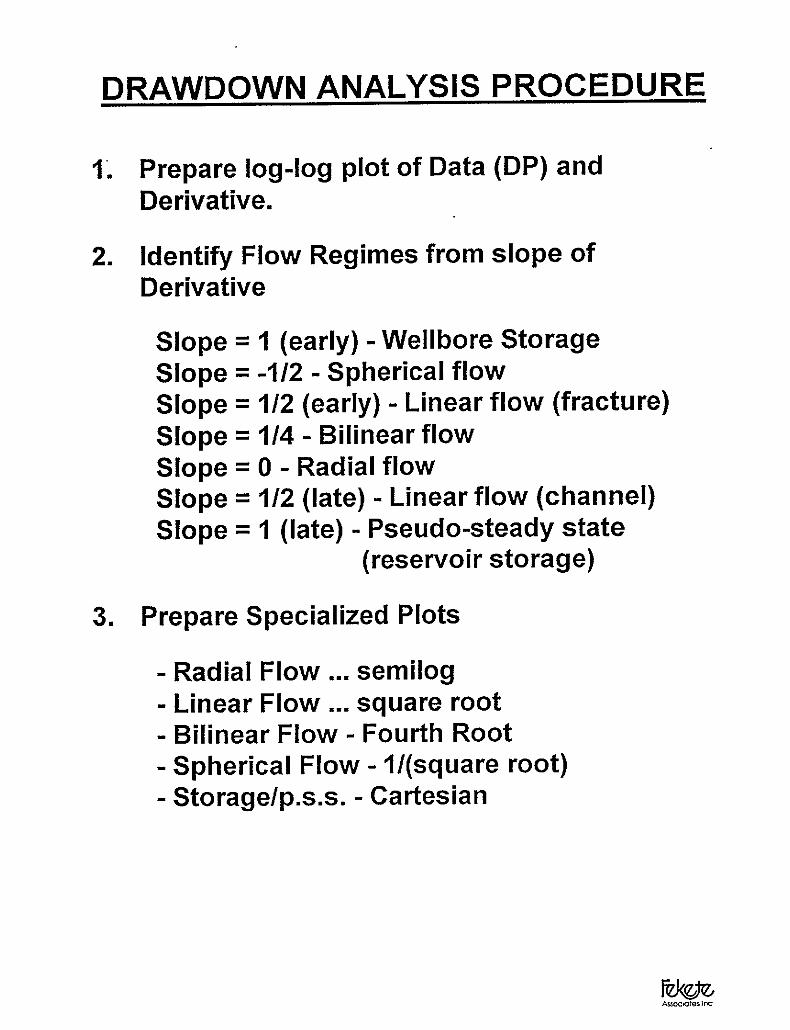
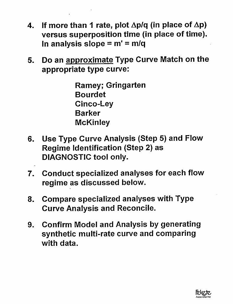
7. Drawdown Analysis (or Injection)a. Procedureb. Specialized Analysesc. Horizontal Wells
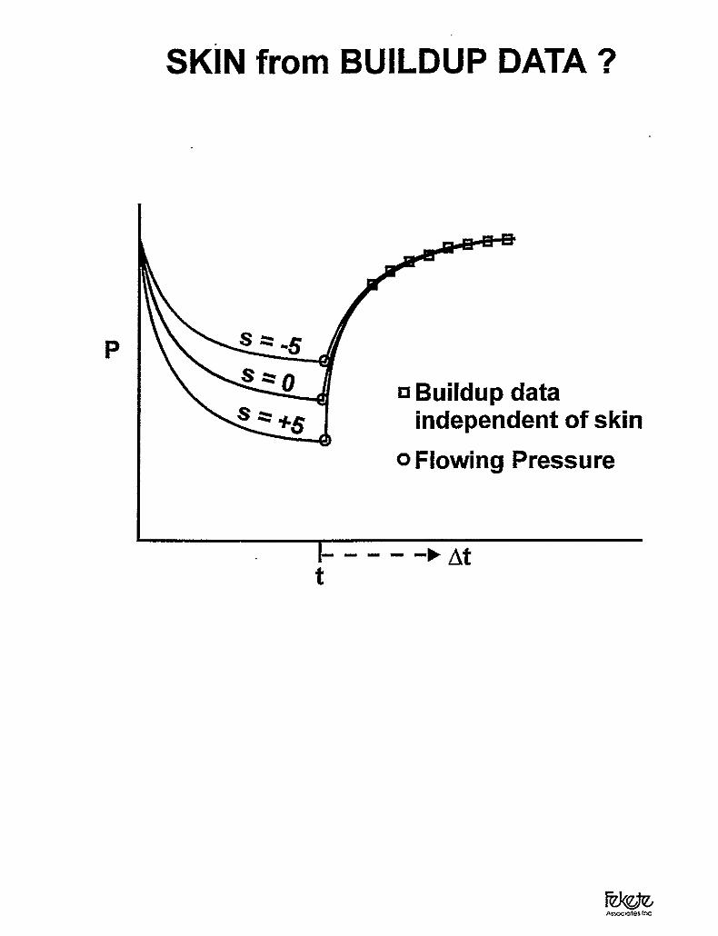
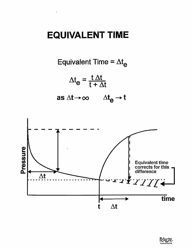
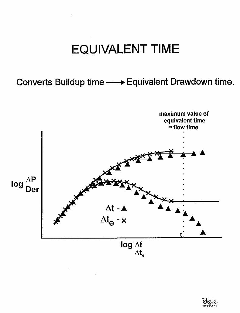
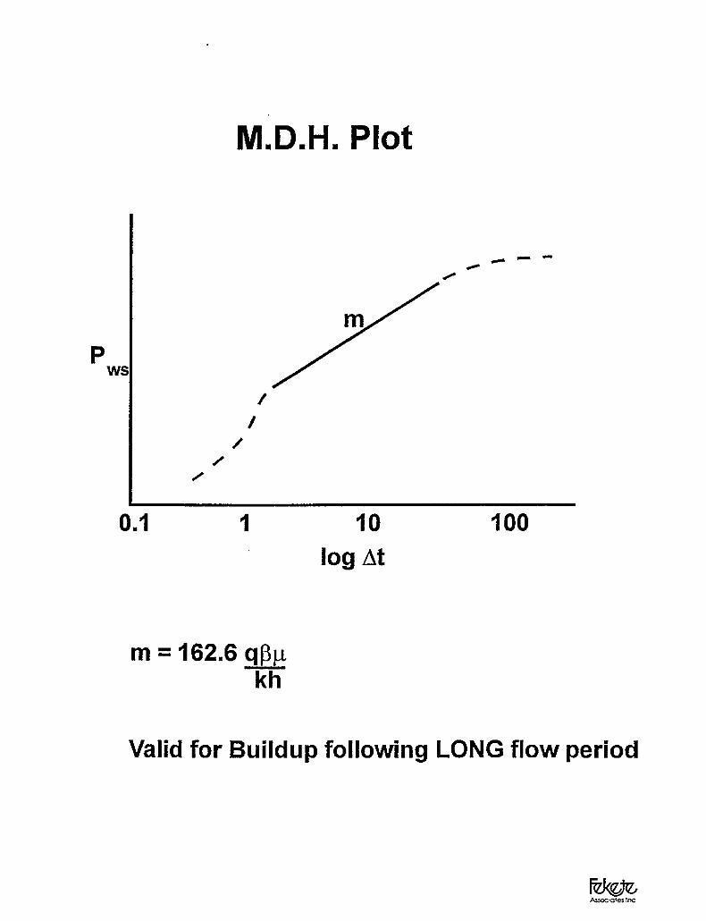
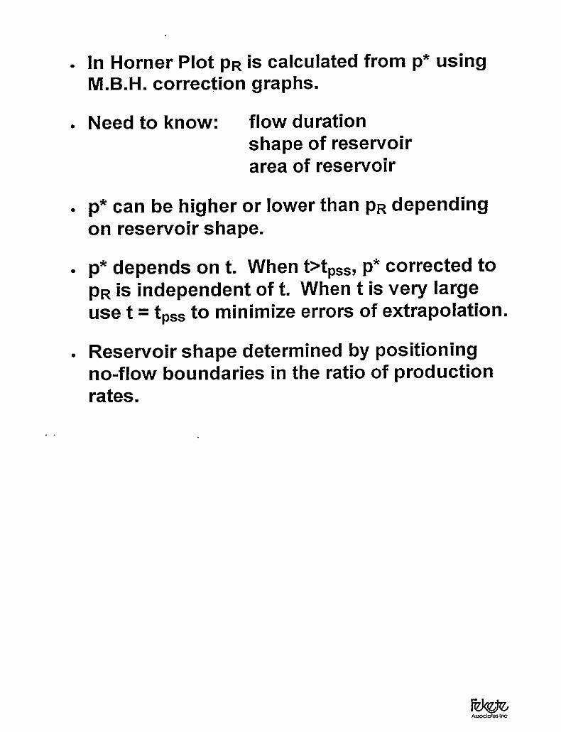
8. Buildup Analysisa. Horner Plotb. Equivalent Timec. M.D.H. Plotd. Average Reservoir Pressuree. Detection of boundariesf. Other Buildup Curvesg. D.S.T.h. Horizontal Wells
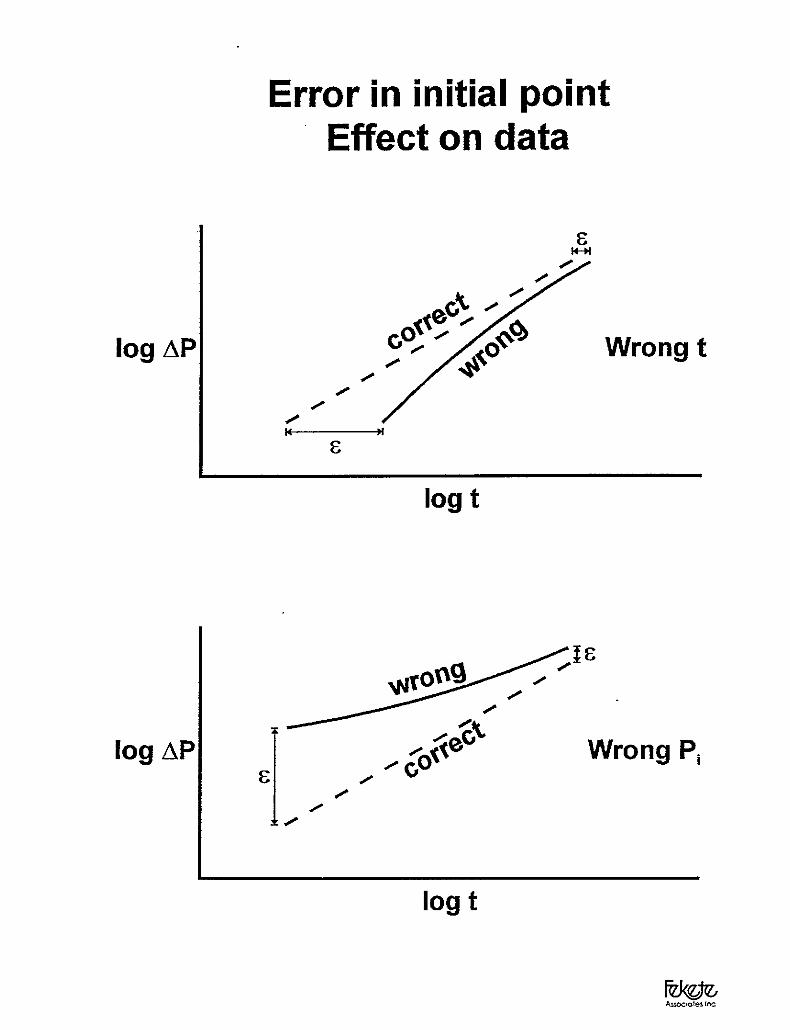
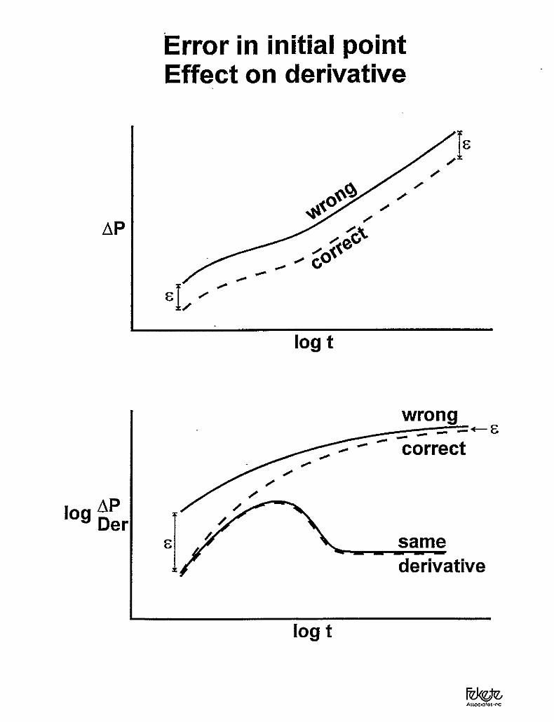
9. Non-Reservoir Effectsa. Data Validationb. Welbore Dynamicsc. Primary Pressure Derivative – PDD
10. Production Forecastinga. Transient/Stabilized IPRb. AOF – Sandface/Wellhead
11. Test Design
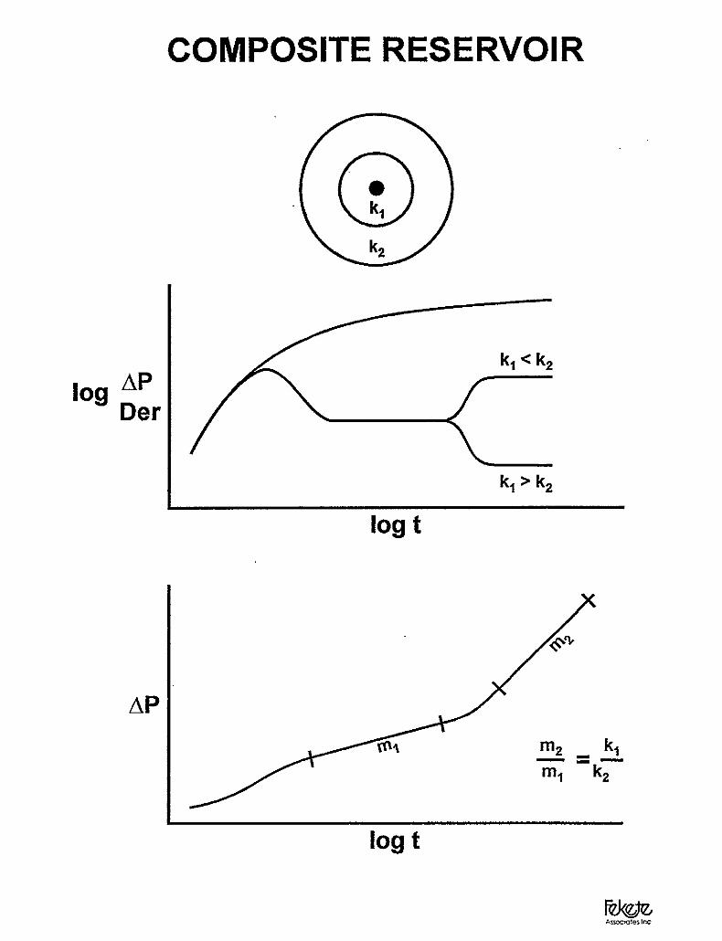
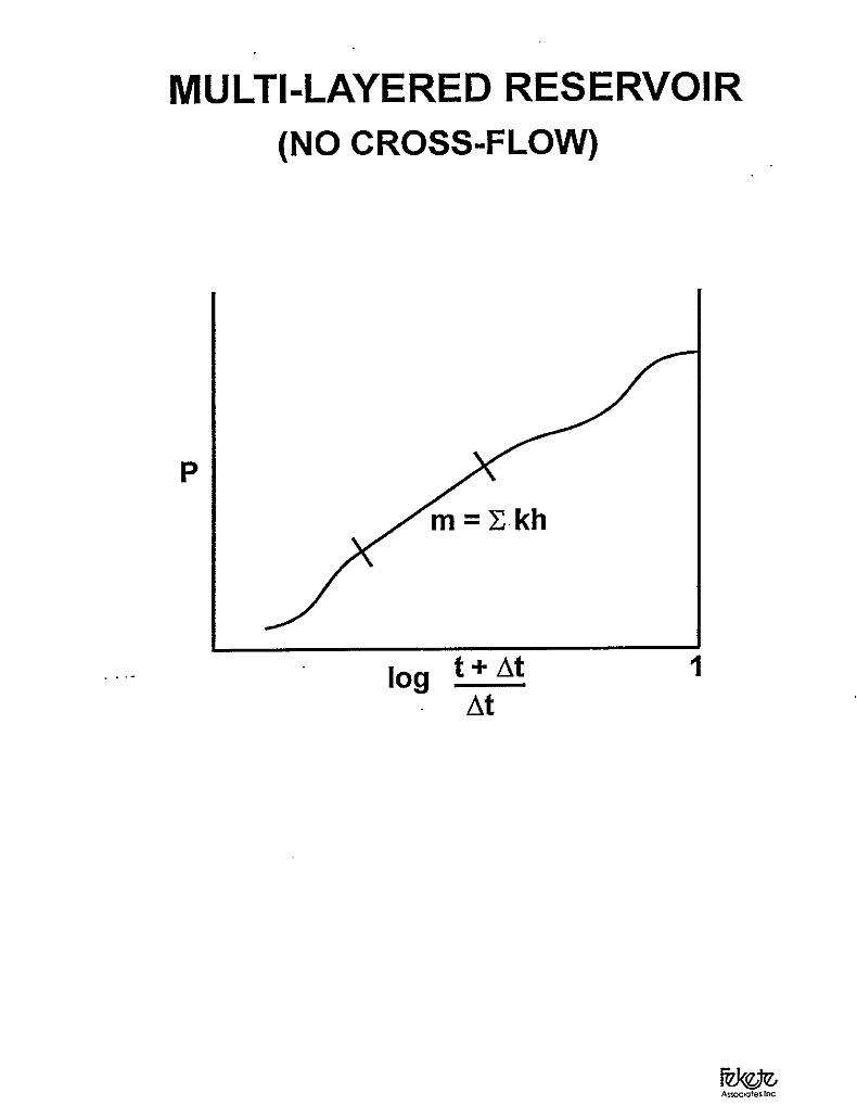
12. Complex Models
13. Pitfalls
14. References/Nomenclature
15. Miscellaneousa. ERCB Chapter 3b. Acoustic Well Soundersc. EUB Guide 40d. Partial Penetratione. Practical Considerations

LOUIS MATTAR, M.Sc., P. Eng.PRESIDENT
Fekete Associates Inc
B.Sc. Honours in Chemical Engineering, University of Wales in Swansea, 1965
M.Sc. in Chemical Engineering, University of Calgary, 1973
Membership: APEGGA; Petroleum Society of CIM; Society of Petroleum Engineers
Louis worked for the Alberta Energy Resources Conservation Board, where he was theprincipal author of the world-renowned E.R.C.B. publication "Theory & Practice of theTesting of Gas Wells, 1975", which is an authoritative text on the subject.
For several years, Louis was Associate Professor at the University of Calgary where hetaught courses in Reservoir Engineering and Advanced Well Testing, and conductedresearch in tight gas reservoirs, and multi-phase flow.
Since 1981 he has been with Fekete Associates, a consulting company that specializesin well testing and reservoir engineering. He has analyzed and supervised theinterpretation of thousands of well tests and specializes in the integration of practicewith theory. He has appeared as an expert witness in several Energy Board hearings.He has conducted studies ranging from shallow gas reservoirs to deep sour wells, fromsmall pools to a 5000-well reservoir/completion/production study, and from waterfloodsto gas storage.
Louis teaches the CIM course in “Gas Well Testing, Theory and Practice”, as well as“Modern Production Decline Analysis” to the SPE and to several companies. He hasauthored 43 technical publications. He is an adjunct professor at the University ofCalgary.
AWARDS:
Louis was the SPE Distinguished Lecturer in Well Testing for 2002-2003. He is aDistinguished Member of the Petroleum Society of CIM. In 1995, he received the CIMDistinguished Author award and the Outstanding Service award. In 1987, he receivedthe CIM District 5 Technical Proficiency Award.
TECHNICAL PUBLICATIONSBY
LOUIS MATTAR
43. MATTAR, L.: “Analytical Solutions in Well Testing”, Invited Panelist, CIPC PanelDiscussion at the Canadian International Petroleum Conference, Calgary,Alberta, June, 2003.
42. MATTAR, L. and ANDERSON, D.M.: “A Systematic and ComprehensiveMethodology for Advanced Analysis of Production Data”, SPE 84472, presentedat the SPE Annual Technical Conference and Exhibition, Denver, Colorado,October, 2003.
41. RAHMAN, A.N.M., MILLER, M.D., MATTAR, L: “Analytical Solution to theTransient-Flow Problems for a Well Located near a Finite-Conductivity Fault inComposite Reservoirs”, SPE 84295, presented at the SPE Annual TechnicalConference and Exhibition, Denver, Colorado, October, 2003.
40. ANDERSON, D.M. and MATTAR, L.: “Material–Balance–Time During Linearand Radial Flow”, CIPC 2003-201, presented at the Canadian InternationalPetroleum Conference, Calgary, Alberta, June, 2003.
39. ANDERSON, D.M., JORDAN, C.L., MATTAR, L.: “Why Plot the EquivalentTime Derivative on Shut-in Time Coordinates?”, presented at the SPE GasTechnology Symposium, May 2002, Paper number 75703.
38. POOLADI-DARVISH, M. and MATTAR, L.: “SAGD Operations in the Presenceof Overlying Gas Cap and Water Layer-Effect of Shale Layers, CIM 2001-178
37. THOMPSON, T. W. and MATTAR, L.: “Gas Rate Forecasting During Boundary-Dominated Flow”, CIM 2000-46, Canadian International Petroleum Conference2000, Calgary, Alberta, June 2000.
36. JORDAN, C. L. and MATTAR, L.: “Comparison of Pressure Transient Behaviourof Composite and Multi-layered Reservoirs,” presented at the CanadianInternational Petroleum Conference, Calgary, Alberta, June, 2000.
35. MATTAR, L.: “DISCUSSION OF A Practical Method for Improving the Accuracyof Well Test Analyses through Analytical Convergence”, Journal of CanadianPetroleum Technology, May 1999.
34. STANISLAV, J., JIANG, Q. and MATTAR, L.: “Effects of Some SimplifyingAssumptions on Interpretation of Transient Data”, CIM 96-51, 47th AnnualTechnical Meeting of the Petroleum Society of CIM, Calgary, Alberta, June 1998.
33. MATTAR, L. and McNEIL, R. “The Flowing Gas Material Balance”, Journal ofCanadian Petroleum Technology (February, 1998), 52, 55
32. MATTAR, L.: “Derivative Analysis Without Type Curves,” presented at the 48thAnnual Technical Meeting of the Petroleum Society of CIM, Calgary, Alberta,June 8-11, 1997
31. MATTAR, L.: “Computers - Black Box or Tool Box?” Guest Editorial, Journal ofCanadian Petroleum Technology, (March, 1997), 8
30. MATTAR, L.: “How Useful are Drawdown Type Curves in Buildup Analysis?”,CIM 96-49, 47th Annual Technical Meeting of the Petroleum Society of CIM,Calgary, Alberta, June 1996.
29. MATTAR, L. and SANTO, M.S.: “A Practical and Systematic Approach toHorizontal Welltest Analysis”, The Journal of Canadian Petroleum Technology,(November, 1995), 42-46
28. MATTAR, L.: “Optimize Your Gas Deliverability With F.A.S.T. PIPERTM,American Pipeline Magazine, August, 1995, 16-17.
27. MATTAR, L.: “Commingling”, Internal Report26. MATTAR, L.: “Reservoir Pressure Analysis: Art or Science?”, Distinguished
Authors Series, The Journal of Canadian Petroleum Technology, (March, 1995),13-16
25. MATTAR, L.: “Practical Well Test Interpretation”, SPE 27975, University of TulsaCentennial Petroleum Engineering Symposium, Tulsa, OK, U.S.A., Aug., 1994
24. MATTAR, L., HAWKES, R.V., SANTO, M.S. and ZAORAL, K.: "Prediction ofLong Term Deliverability in Tight Formations", SPE 26178, SPE Gas TechnologySymposium, Calgary, Alberta, June, 1993
23. MATTAR, L.: "Critical Evaluation and Processing of Data Prior to PressureTransient Analysis," presented at the 67th Annual Technical Conference andExhibition of the Society of Petroleum Engineers, Washington, D.C., October 4-7,1992
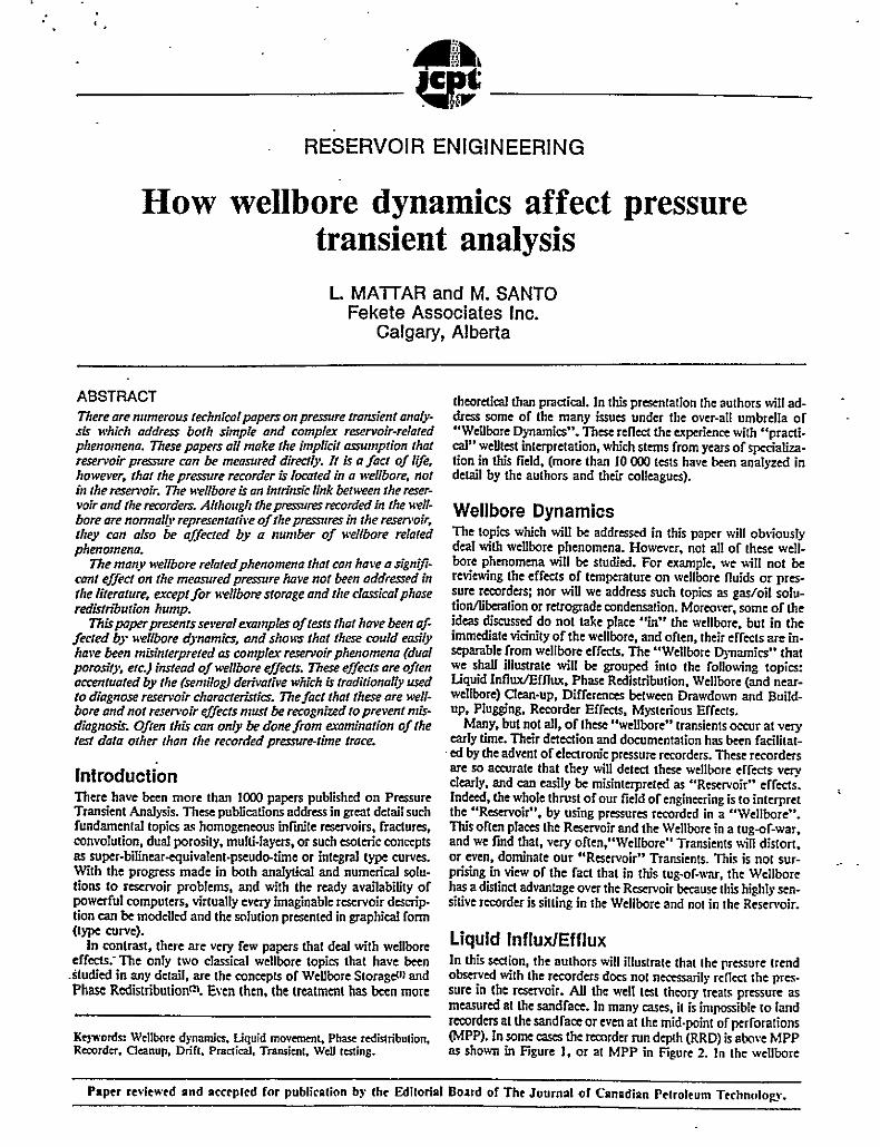
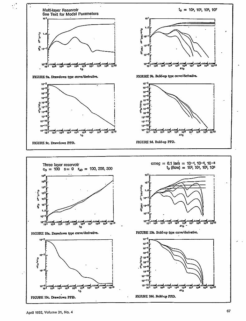
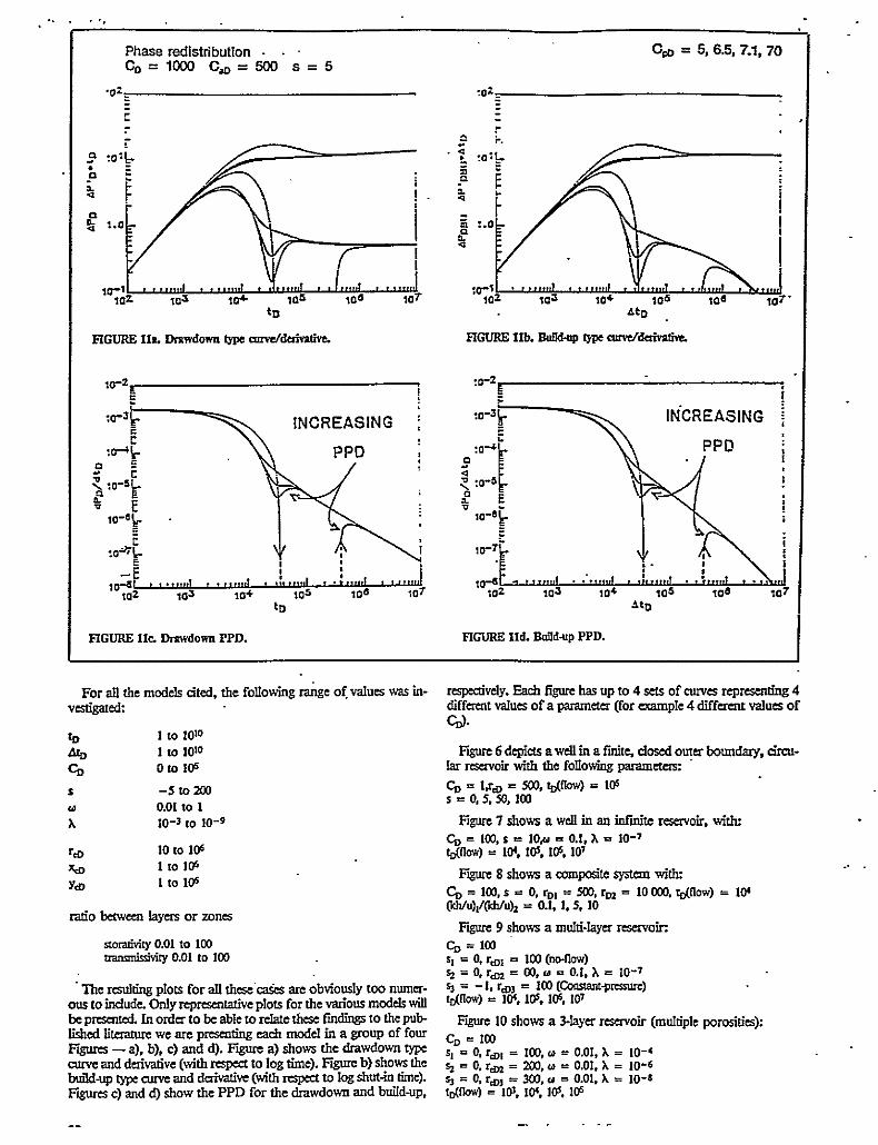
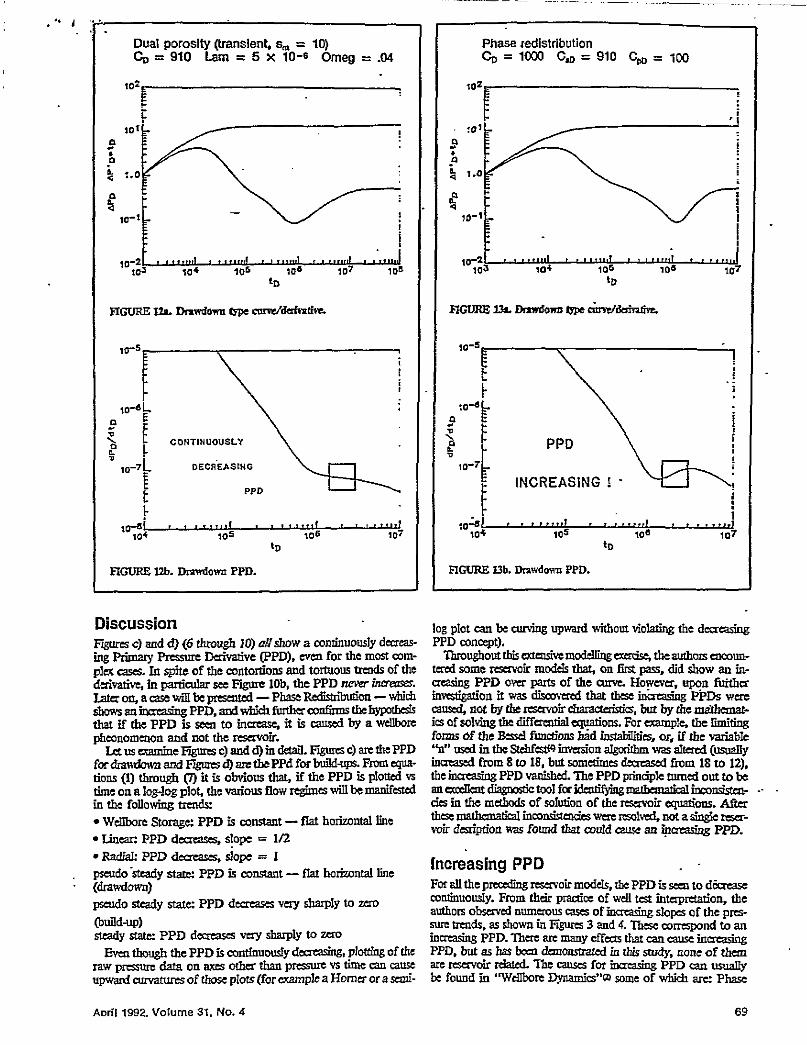
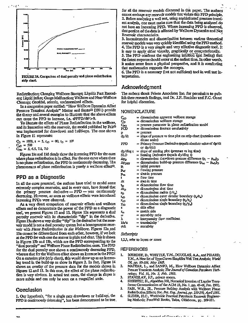
22. MATTAR, L. and SANTO, M.S.: "How Wellbore Dynamics Affect PressureTransient Analysis," The Journal of Canadian Petroleum Technology, Vol. 31,No. 2, February, 1992
21. MATTAR, L. and ZAORAL, K.: "The Primary Pressure Derivative (PPD) - A NewDiagnostic Tool in Well Test Interpretation," The Journal of Canadian PetroleumTechnology, Vol. 31, No. 4, April, 1992
20. ABOU-KASSEM, J.H., MATTAR, L. and DRANCHUK, P.M.: "ComputerCalculations of Compressibility of Natural Gas", Journal of Canadian PetroleumTechnology, Calgary, Alberta, Sep.-Oct. 1990, Vol. 29 No. 5 p. 105
19. MATTAR, L.: "IPR's and All That - The Direct and Inverse Problem", PreprintPaper No. 87-38-13, 38th Annual Technical Meeting of the Petroleum Society ofCIM, Calgary, Alberta, June 1987
18. BRAR, G.S. and MATTAR, L.: "Reply to Discussion of: The Analysis of ModifiedIsochronal Tests to predict the Stabilized Deliverability of Gas Wells withoutUsing Stabilized Flow Data", The Journal of Petroleum Technology, AIME(January, 1987), 89-92
17. LAIRD, A.D. and MATTAR, L.: "Practical Well Test Design to Evaluate HydraulicFractures in Low Permeability Wells", Preprint Paper No. 85-36-8, 36th AnnualTechnical Meeting of the Petroleum Society of CIM, Edmonton, Alberta, June1985
16. MATTAR, L. and ZAORAL, K.: "Gas Pipeline Efficiencies and Pressure GradientCurves", Preprint Paper No. 84-35-93, 35th Annual Technical Meeting of thePetroleum Society of CIM, Calgary, Alberta, June 1984
15. MATTAR, L. and HAWKES, R.V.: "Start of the Semi-Log Straight Line in BuildupAnalysis", Preprint Paper No. 84-35-92, 35th Annual Technical Meeting of thePetroleum Society of CIM, Calgary, Alberta, June 1984
14. WASSON, J. and MATTAR, L.: "Problem Gas Well Build-Up Tests - A FieldCase Illustration of Solution Through the Use of Combined Techniques", TheJournal of Canadian Petroleum Technology (March - April, 1983), 36-54
13. NUTAKKI, R. and MATTAR, L.: "Pressure Transient Analysis of Wells in VeryLong Narrow Reservoirs", Preprint Paper No. SPE 1121, 57th Annual FallTechnical Conference and Exhibition of the Society of Petroleum Engineers ofAIME, New Orleans, LA, September 1982
12. LIN, C. and MATTAR, L.: "Determination of Stabilization Factor and Skin Factorfrom Isochronal and Modified Isochronal Tests", The Journal of CanadianPetroleum Technology (March - April, 1982), 89-94
11. MATTAR, L. and LIN, C.: "Validity of Isochronal and Modified Isochronal Testingof Gas Wells", Preprint Paper SPE 10126, 56th Annual Fall TechnicalConference of AIME, San Antonio, TX, October 1981
10. KALE, D. and MATTAR, L.: "Solution of a Non-Linear Gas Flow Equation by thePerturbation Technique", The Journal of Canadian Petroleum Technology(October-December, 1980), 63-67
9. ADEGBESAN, K.O. and MATTAR, L.: "Prediction of Pressure Drawdown in GasReservoirs Using a Semi-Analytical Solution of the Non-Linear Gas FlowEquation", Preprint Paper No. 80-31-39, 31st Annual Technical Meeting of theSociety of CIM, Calgary, Alberta, May 198077. MATTAR, L.: “Variation ofViscosity-Compressibility Product With Pressure of Natural Gas", Internal Report,1980
8. MATTAR, L.: “Variation of Viscosity-Compressibility Product With Pressure ofNatural Gas", Internal Report, 1980
7. MATTAR, L., NICHOLSON, M., AZIZ, K. and GREGORY, G.: "Orifice Meteringof Two-Phase Flow", The Journal of Petroleum Technology, AIME (August,1979), 955-961
6. AZIZ, K., MATTAR, L., KO, S. and BRAR, G.: "Use of Pressure, PressureSquared or Pseudo-Pressure in the Analysis of Transient Pressure DrawdownData from Gas Wells", The Journal of Canadian Petroleum Technology, (April -June, 1976), 1-8
5. MATTAR, L., BRAR, G.S. and AZIZ, M.: "Compressibility of Natural Gases", TheJournal of Canadian Petroleum Technology, (October-December, 1975), 77-80
4. E.R.C.B. (1975), "Theory and Practice of the Testing of Gas Wells, Third Edition"(co-authored by L. MATTAR) Alberta Energy Resources Conservation Board,Calgary
3. MATTAR, L. and GREGORY, G.: "Air-Oil Slug Flow in An Upward-Inclined Pipe- 1: Slug Velocity, Holdup and Pressure Gradient", The Journal of CanadianPetroleum Technology, (January - March, 1974), 1-8
2. GREGORY, G. and MATTAR, L.: "An In-Situ Volume Fraction Sensor for TwoPhase Flows of Non-Electrolytes", The Journal of Canadian PetroleumTechnology, (April - June, 1973), 1-5
1. MATTAR, L.: "Slug Flow Uphill In an Inclined Pipe", M.Sc. Thesis, University ofCalgary, Alberta, 1973
EXPERT WITNESS TESTIMONY
LOUIS MATTAR, P.Eng
Appeared before National Energy Board / Alberta Energy Utilities Board to giveevidence and testimony relating to oil and gas issues on several occasions to represent:
i) NOVA Corporation of Albertaii) Merland Exploration Limitediii) GasCan Resources Ltd.iv) Bralorne Resources Limitedv) Encor Inc.vi) Norcen Energy Resources Ltd.vii) Gulf Canada Resources Ltd.viii) Paramount Resourcesix) Devon Canada Incx) Rio Altoxi) Alberta Energy Company
Appeared before the Alberta Court of Queens Bench, as an expert, to represent:
i) Novalta Resources Ltd.


1
1. Traditional (Arps)
2. Fetkovich
3. Blasingame
4. Agarwal-Gardner
5. NPI - Normalized Pressure Integral
6. Modeling
2
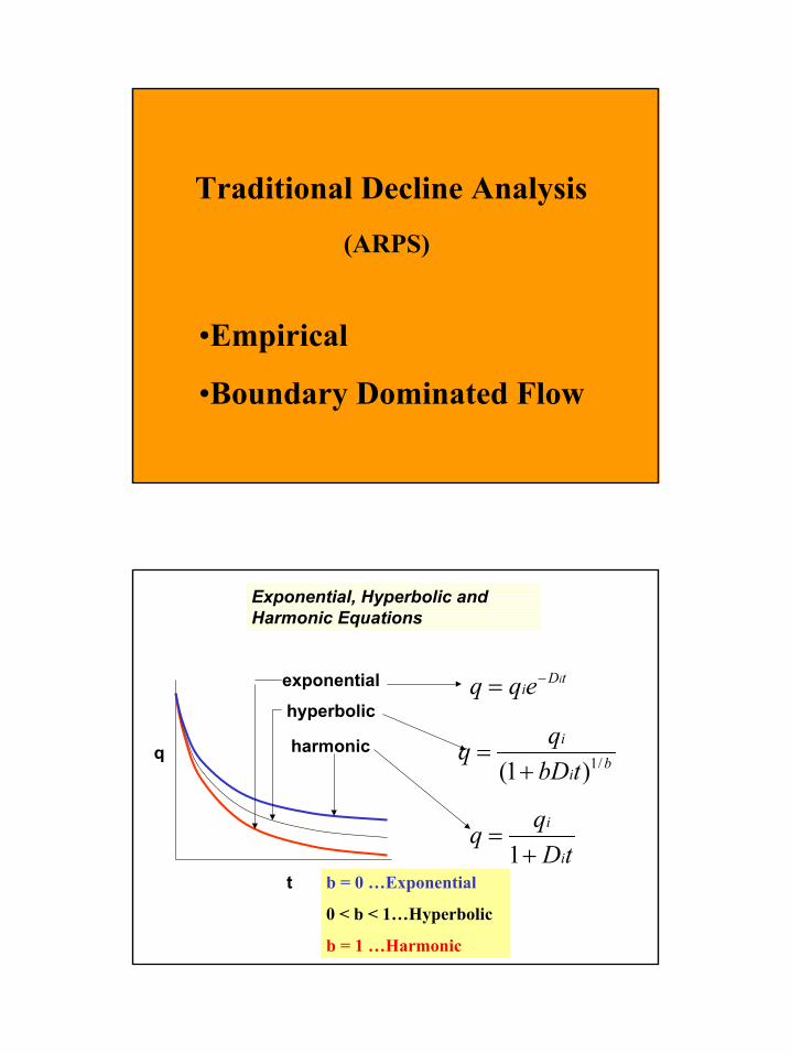
Traditional Decline Analysis
(ARPS)
•Empirical
•Boundary Dominated Flow
Exponential, Hyperbolic andHarmonic Equations
tDqq
i
i
+=
1
q
t
tDi
ieqq −=
bi
i
tbDqq /1)1( +
=
exponential
hyperbolic
harmonic
b = 0 …Exponential
0 < b < 1…Hyperbolic
b = 1 …Harmonic
3
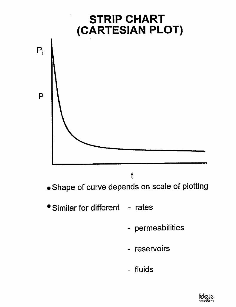
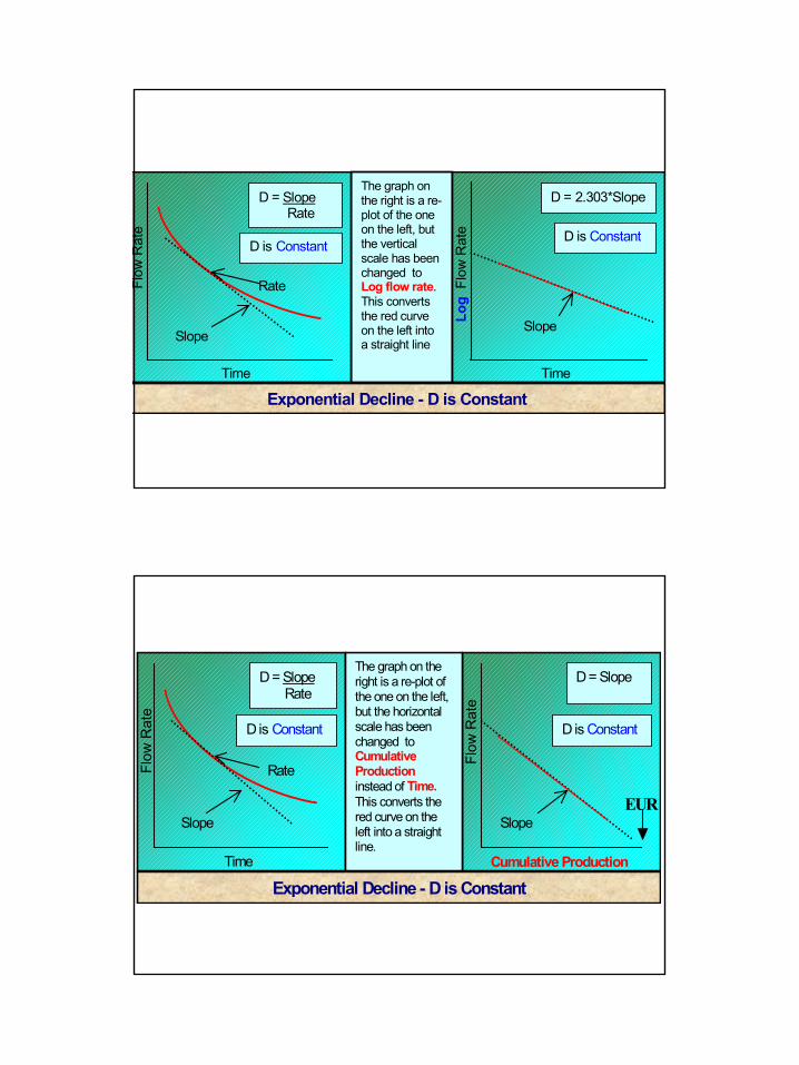
The graph onthe right is a re-plot of the oneon the left, butthe verticalscale has beenchanged toLog flow rate.This convertsthe red curveon the left intoa straight line
Flow
Rat
e
Time
Slope
Rate
D = Slope Rate
Log
Flo
w R
ate
Time
Slope
D = 2.303*Slope
D is ConstantD is Constant
Exponential Decline - D is Constant
Flow
Rat
e
Time
Slope
Rate
D = Slope Rate
Flo
w R
ate
Cumulative Production
Slope
D = SlopeThe graph on theright is a re-plot ofthe one on the left,but the horizontalscale has beenchanged toCumulativeProductioninstead of Time.This converts thered curve on theleft into a straightline.
D is ConstantD is Constant
Exponential Decline - D is Constant
EUR
4
qdt
dqqKD −== 0*
∫∫ −=q
q
t
i qdqDdt
0
iqqDt ln=−
Dti eqq −= *
qdt
dqqKD b −== *
bi
qDK =
∫∫ +−= t
i
q
q b
t
bi
i
qdqdt
qD
10*
bi
bb
i
i qqq
tbD −− −=
( ) bii tbDqq1
1−
+=
qdt
dqqKD −== 1*
i
i
qDK =
∫∫ −=q
q
t
i
i
i qdqdt
qD
20
tii
i
qqqtD 11
−=
( ) 11 −+= tDqq ii
dteqdtqQt t Dt
i ***0 0∫ ∫ −==
DeqqQ
Dtii
−−=
*
qeq Dti =−*
DqqiQ −
=
dttbDqdtqQt t
bii *)1(*
0 0
1
∫ ∫−
+==
−+
−=
−
1)1()1(
1b
b
ii
i tbDDb
bi
i qqtbD
=+ )1(
( ) ( )bbi
i
bi qq
DbqQ −− −−
= 11
1
dttDqdtqQt t
ii *)1(*0 0
1∫ ∫ −+==
[ ]tDDqQ i
i
i += 1ln(
( )qqtD i
i =+1
DqQ i
i
i ln=
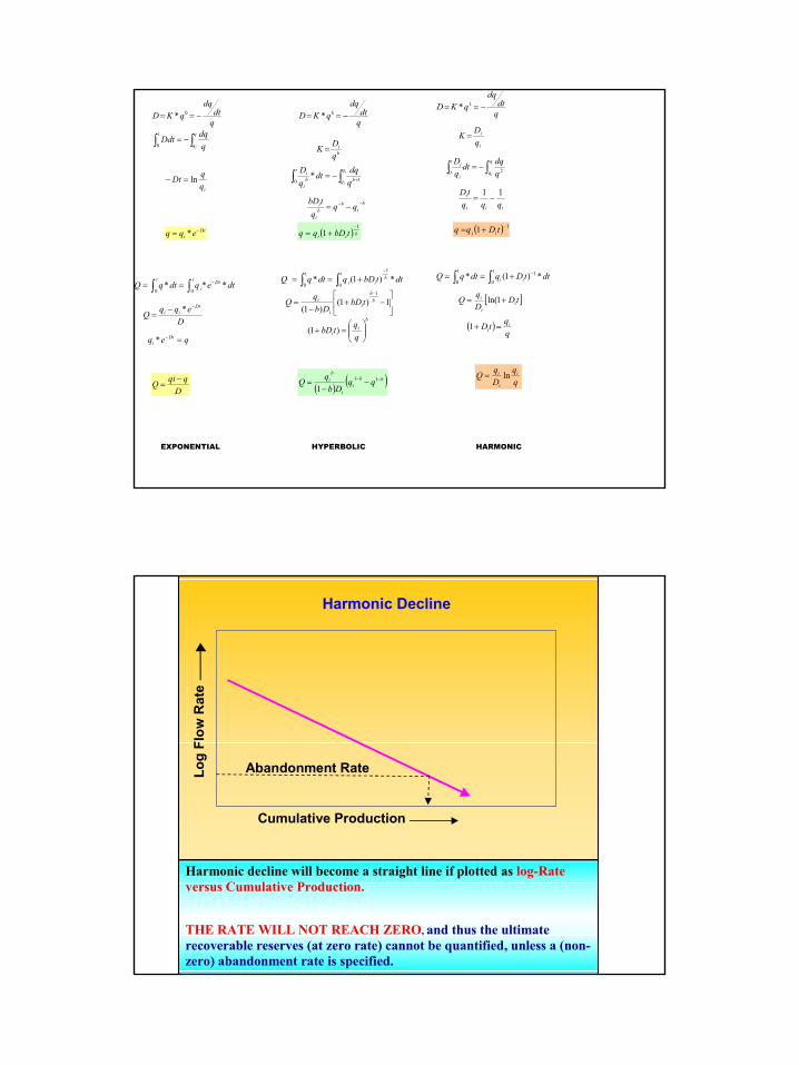
EXPONENTIAL HYPERBOLIC HARMONIC
Harmonic Decline
Cumulative Production
Log
Flow
Rat
e
Harmonic decline will become a straight line if plotted as log-Rateversus Cumulative Production.
THE RATE WILL NOT REACH ZERO, and thus the ultimaterecoverable reserves (at zero rate) cannot be quantified, unless a (non-zero) abandonment rate is specified.
Abandonment Rate

5
Fetkovich
Early TimeTransient
Late TimeBoundary-Dominated
•Constant Operating Conditions
Fetkovich Theory
-Developed because traditional decline curveanalysis is only applicable when well is inboundary dominated flow
- Fetkovich used analytical flow equations togenerate typecurves for transient flow, andcombined them with emprical decline curveequations from Arps
-Resulting typecurves encompass wholeproduction life of well
6
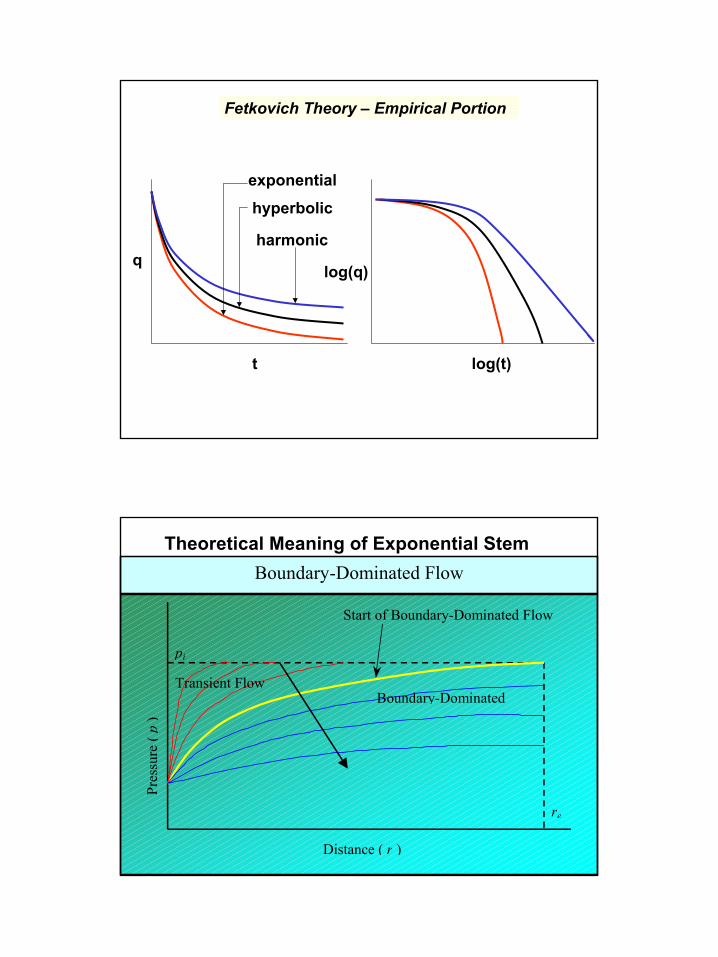
Fetkovich Theory – Empirical Portion
q
t
exponential
hyperbolic
harmonic
log(q)
log(t)
Boundary-Dominated Flow
Distance ( r )
Pres
sure
( p
)
re
pi
Transient FlowBoundary-Dominated
Start of Boundary-Dominated Flow
Theoretical Meaning of Exponential Stem
7
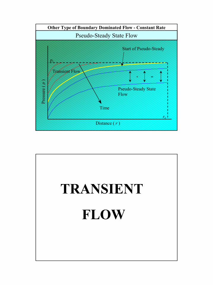
Pseudo-Steady State Flow
Distance ( r )
Pres
sure
( p
)
pi
re
Transient Flow
Start of Pseudo-Steady
Pseudo-Steady StateFlow
= =
Time
Other Type of Boundary Dominated Flow - Constant Rate
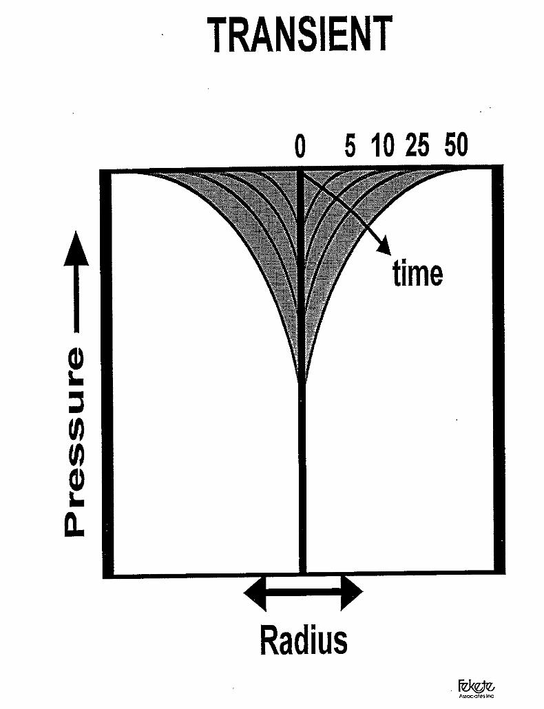
TRANSIENT
FLOW
8
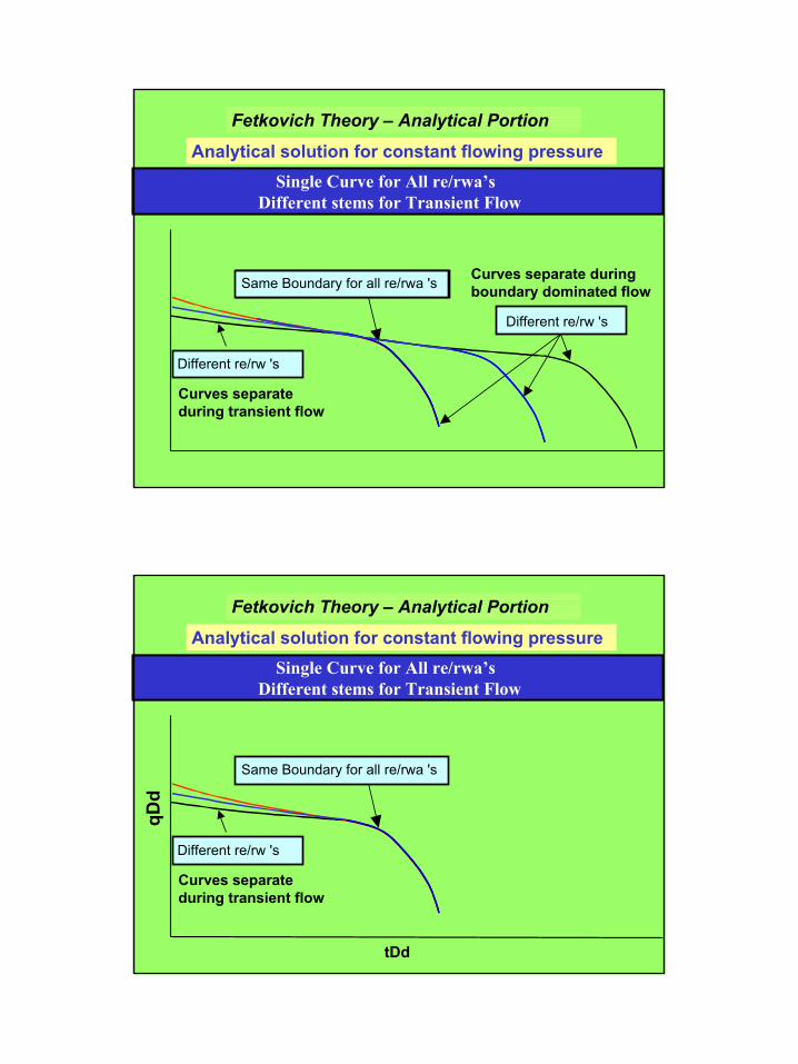
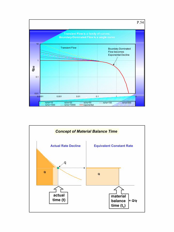
Transient Flow is a single curve;Boundary-Dominated Flow is a family of curves
Different re/rw 's
Curves separate duringboundary dominated flow
Fetkovich Theory – Analytical Portion
Analytical solution for constant flowing pressure
Different re/rw 's
Curves separateduring transient flow
Same Transient for all re/rwa 'sSame Boundary for all re/rwa 's
Different stems for Transient FlowSingle Curve for All re/rwa’s
qDd
tDd
Transient Flow is a single curve;Boundary-Dominated Flow is a family of curves
Fetkovich Theory – Analytical Portion
Analytical solution for constant flowing pressure
Different re/rw 's
Curves separateduring transient flow
Same Boundary for all re/rwa 's
Different stems for Transient FlowSingle Curve for All re/rwa’s
9
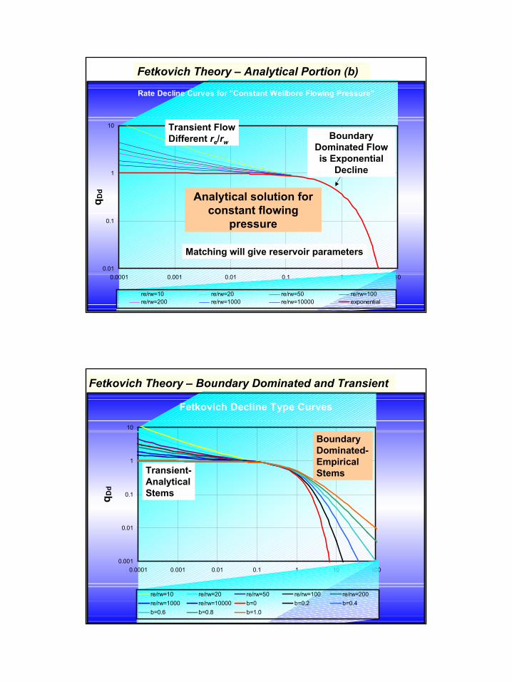
Rate Decline Curves for "Constant Wellbore Flowing Pressure"
0.01
0.1
1
10
0.0001 0.001 0.01 0.1 1 10tDd
q Dd
re/rw=10 re/rw=20 re/rw=50 re/rw=100re/rw=200 re/rw=1000 re/rw=10000 exponential
Transient Flow Boundary Dominated Flow becomes Exponential Decline
Fetkovich Theory – Analytical Portion (b)
Analytical solution forconstant flowing
pressure
Transient FlowDifferent re/rw
BoundaryDominated Flowis Exponential
Decline
Matching will give reservoir parameters
Fetkovich Decline Type Curves
0.001
0.01
0.1
1
10
0.0001 0.001 0.01 0.1 1 10 100tDd
q Dd
re/rw=10 re/rw=20 re/rw=50 re/rw=100 re/rw=200re/rw=1000 re/rw=10000 b=0 b=0.2 b=0.4b=0.6 b=0.8 b=1.0
Fetkovich Theory – Boundary Dominated and Transient
Transient-AnalyticalStems
BoundaryDominated-EmpiricalStems
10
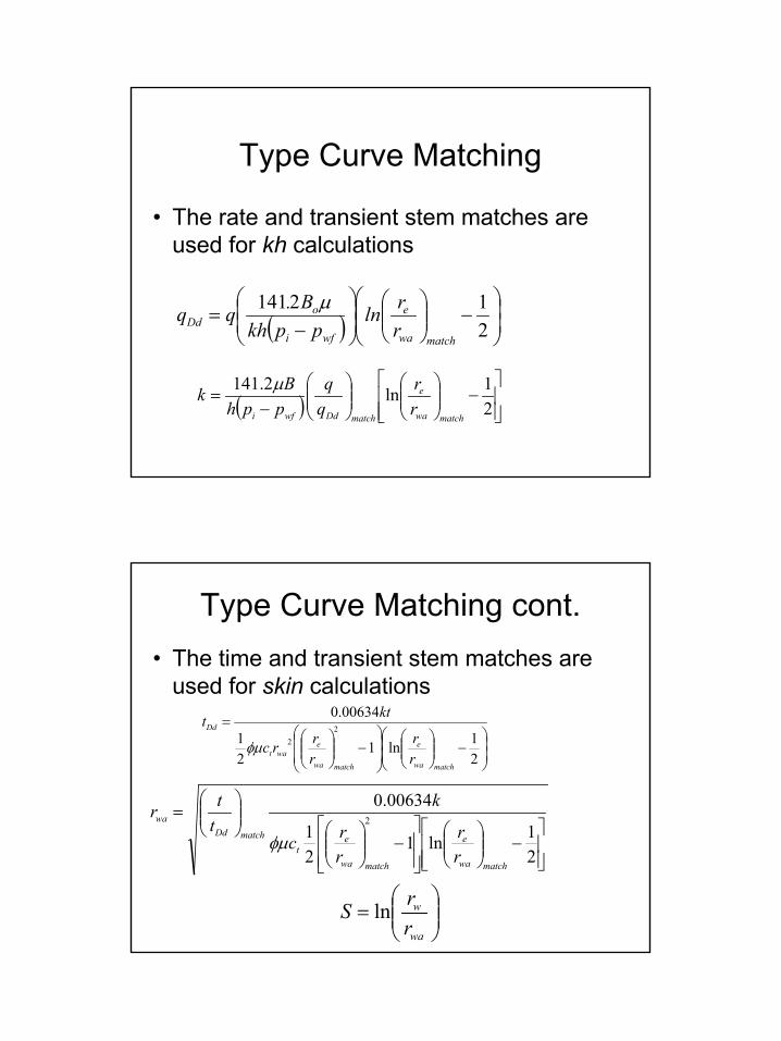
Type Curve Matching
• The rate and transient stem matches areused for kh calculations
( )
−
−=
212141
matchwa
e
wfi
oDd r
rlnppkh
B.qq µ
( )
−
−
=21ln2.141
matchwa
e
matchDdwfi rr
pphBk µ
Type Curve Matching cont.• The time and transient stem matches are
used for skin calculations
−
−
=
21ln1
21
00634.02
matchwa
e
matchwa
et
matchDdwa
rr
rrc
kttr
φµ
−
−
=
21ln1
21
00634.02
2
matchwa
e
matchwa
ewat
Dd
rr
rrrc
ktt
φµ
=
wa
w
rrS ln
11
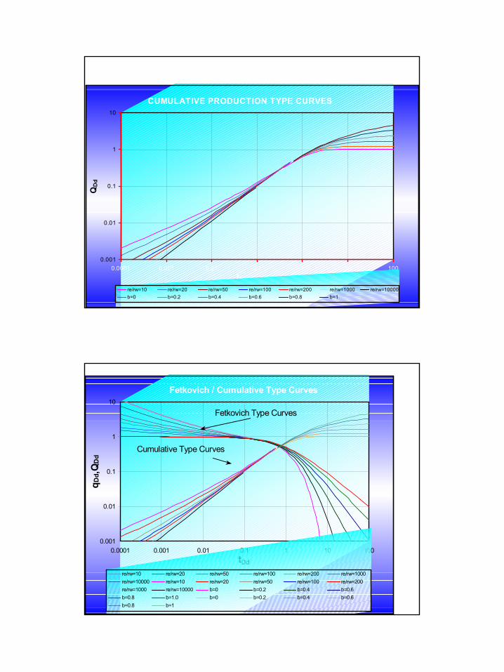
0.001
0.01
0.1
1
10
0.0001 0.001 0.01 0.1 1 10 100tDd
QD
d
re/rw=10 re/rw=20 re/rw=50 re/rw=100 re/rw=200 re/rw=1000 re/rw=10000b=0 b=0.2 b=0.4 b=0.6 b=0.8 b=1
CUMULATIVE PRODUCTION TYPE CURVES
0.001
0.01
0.1
1
10
0.0001 0.001 0.01 0.1 1 10 100tDd
q Dd,Q
Dd
re/rw=10 re/rw=20 re/rw=50 re/rw=100 re/rw=200 re/rw=1000re/rw=10000 re/rw=10 re/rw=20 re/rw=50 re/rw=100 re/rw=200re/rw=1000 re/rw=10000 b=0 b=0.2 b=0.4 b=0.6b=0.8 b=1.0 b=0 b=0.2 b=0.4 b=0.6b=0.8 b=1
Fetkovich / Cumulative Type Curves
Cumulative Type Curves
Fetkovich Type Curves
12
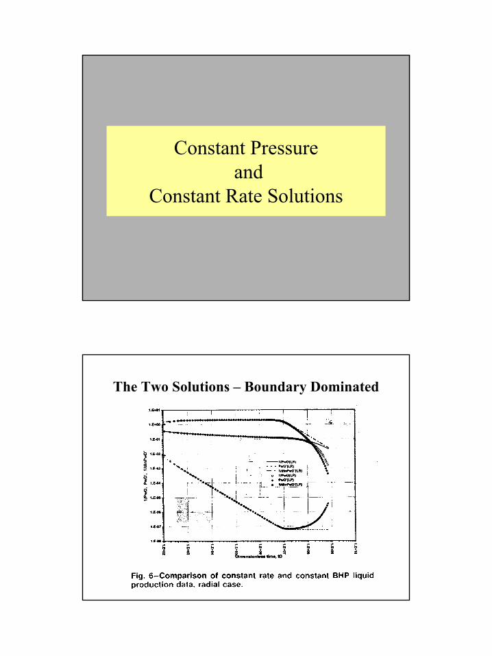
Constant Pressure and
Constant Rate Solutions
The Two Solutions – Boundary Dominated
13
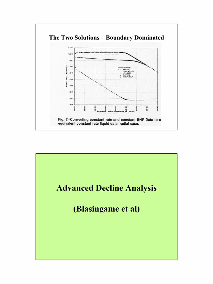
The Two Solutions – Boundary Dominated
Advanced Decline Analysis
(Blasingame et al)
14
Transient Flow is a family of curves;Boundary-Dominated Flow is a single curve
0.01
0.1
1
10
0.0001 0.001 0.01 0.1 1 10tDd
q Dd
re/rw=10 re/rw=20 re/rw=50 re/rw=100 re/rw=200re/rw=1000 re/rw=10000 exponential
Transient Flow Boundary Dominated Flow becomes Exponential Decline
P.54
Actual Rate Decline Equivalent Constant Rate
q
Q
actualtime (t)
Q
Concept of Material Balance Time
= Q/qmaterialbalancetime (tc)
15
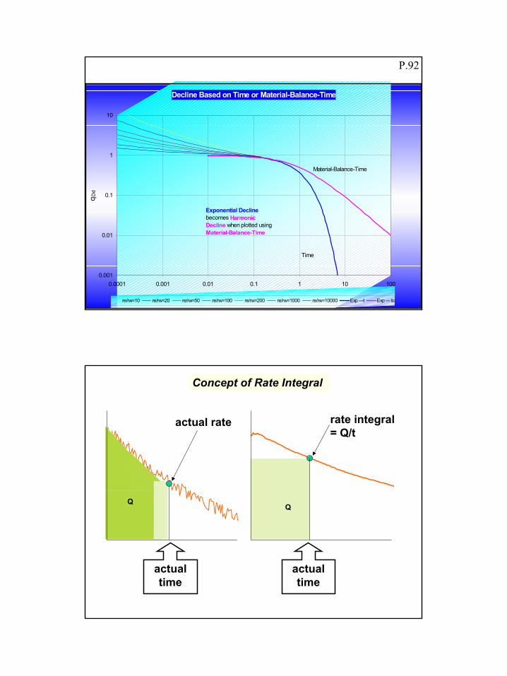
Decline Based on Time or Material-Balance-Time
0.001
0.01
0.1
1
10
0.0001 0.001 0.01 0.1 1 10 100tDd, tcDd
qDd
re/rw=10 re/rw=20 re/rw=50 re/rw=100 re/rw=200 re/rw=1000 re/rw=10000 Exp ---t Exp --- tc
Time
Material-Balance-Time
Exponential Decline becomes Harmonic Decline when plotted using Material-Balance-Time
P.92
actual rate
Q
actualtime
Q
Concept of Rate Integral
rate integral= Q/t
actualtime
16
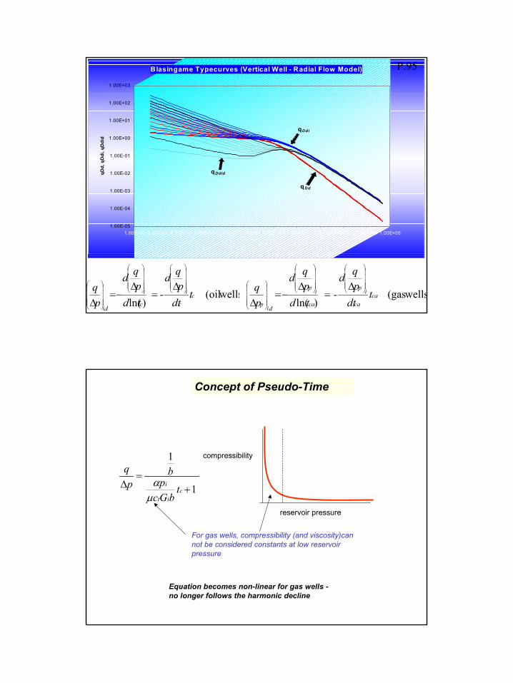
wells(oil )ln(
cc
i
c
i
di
tdt
pqd
-tdpqd
pq
∆=
∆−=
∆ wells(gas
)ln(ca
ca
ip
ca
ip
dip
tdt
pqd
-tdpqd
pq
∆=
∆−=
∆
Blasingame Typecurves (Vertical Well - Radial Flow Model)
1.00E-05
1.00E-04
1.00E-03
1.00E-02
1.00E-01
1.00E+00
1.00E+01
1.00E+02
1.00E+03
1.00E-06 1.00E-05 1.00E-04 1.00E-03 1.00E-02 1.00E-01 1.00E+00 1.00E+01 1.00E+02 1.00E+03 1.00E+04 1.00E+05
tDd
qDd,
qD
di, q
Ddi
d
qDdi
qDdid
qDd
P.95
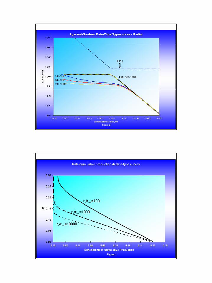
Concept of Pseudo-Time
1
1
+=
∆c
it
i tbGc
pb
pq
µα
For gas wells, compressibility (and viscosity)cannot be considered constants at low reservoirpressure
compressibility
reservoir pressure
Equation becomes non-linear for gas wells -no longer follows the harmonic decline
17
18
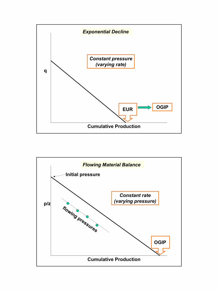
q
EUR
Exponential Decline
Constant pressure(varying rate)
Cumulative Production
OGIP
Initial pressure
Cumulative Production
p/z
OGIP
flowing pressures
Flowing Material Balance
Constant rate(varying pressure)
19
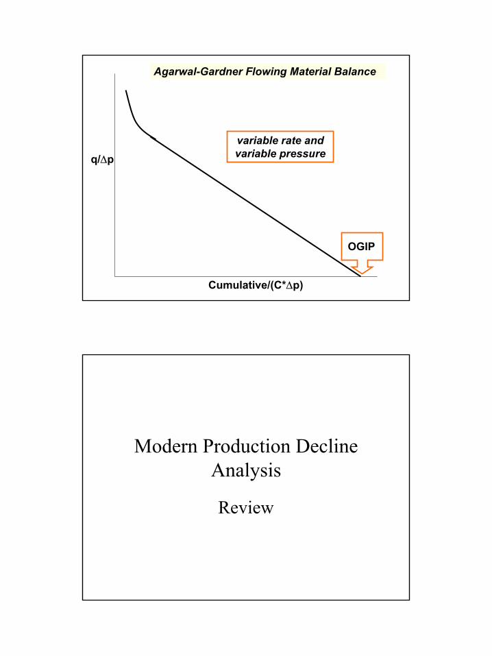
Cumulative/(C*∆p)
q/∆p
OGIP
Agarwal-Gardner Flowing Material Balance
variable rate andvariable pressure
Modern Production DeclineAnalysis
Review
20
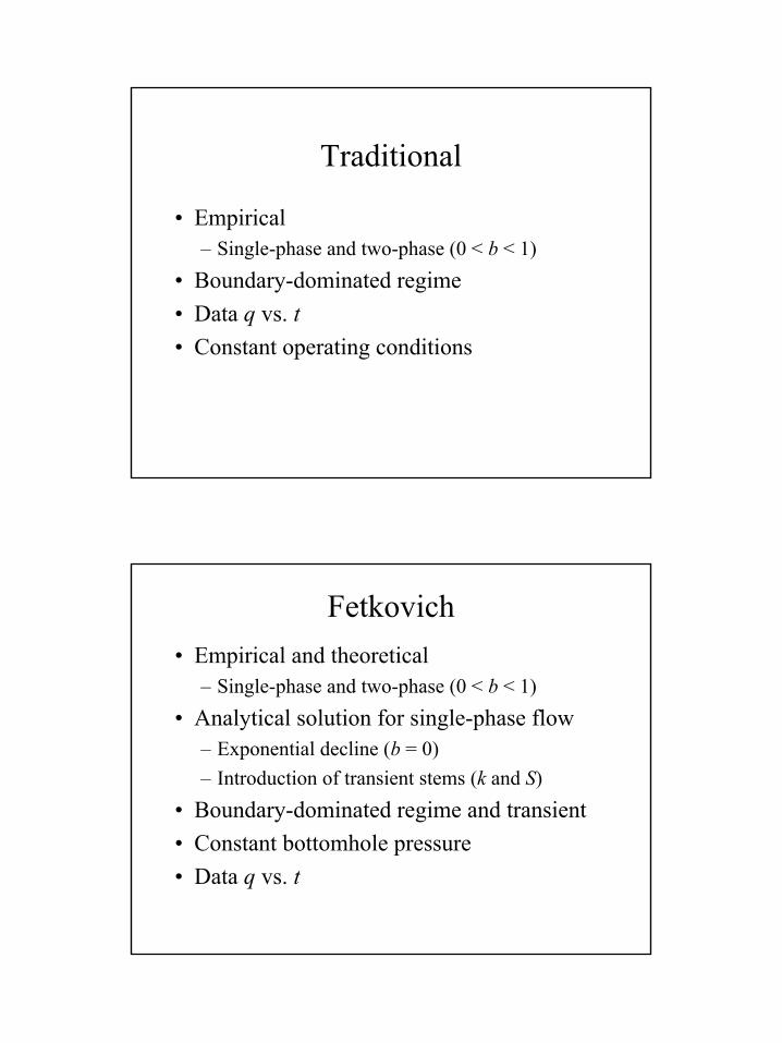
Traditional
• Empirical– Single-phase and two-phase (0 < b < 1)
• Boundary-dominated regime• Data q vs. t• Constant operating conditions
Fetkovich• Empirical and theoretical
– Single-phase and two-phase (0 < b < 1)• Analytical solution for single-phase flow
– Exponential decline (b = 0)– Introduction of transient stems (k and S)
• Boundary-dominated regime and transient• Constant bottomhole pressure• Data q vs. t
21
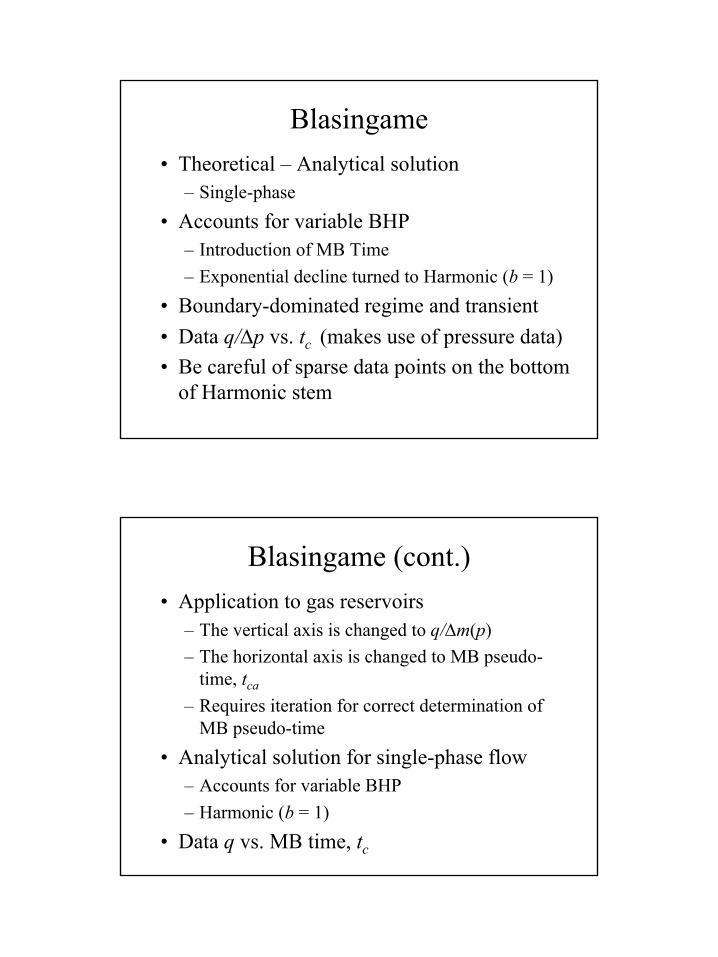
Blasingame• Theoretical – Analytical solution
– Single-phase• Accounts for variable BHP
– Introduction of MB Time– Exponential decline turned to Harmonic (b = 1)
• Boundary-dominated regime and transient• Data q/∆p vs. tc (makes use of pressure data)• Be careful of sparse data points on the bottom
of Harmonic stem
Blasingame (cont.)• Application to gas reservoirs
– The vertical axis is changed to q/∆m(p)– The horizontal axis is changed to MB pseudo-
time, tca
– Requires iteration for correct determination ofMB pseudo-time
• Analytical solution for single-phase flow– Accounts for variable BHP– Harmonic (b = 1)
• Data q vs. MB time, tc
22
Agarwal Gardner
• Uses the same data as Blasingame– The same analysis techniques and plotting
apply• The flowing material balance plot allows an
alternative representation of data– Very advantageous for determination of OGIP

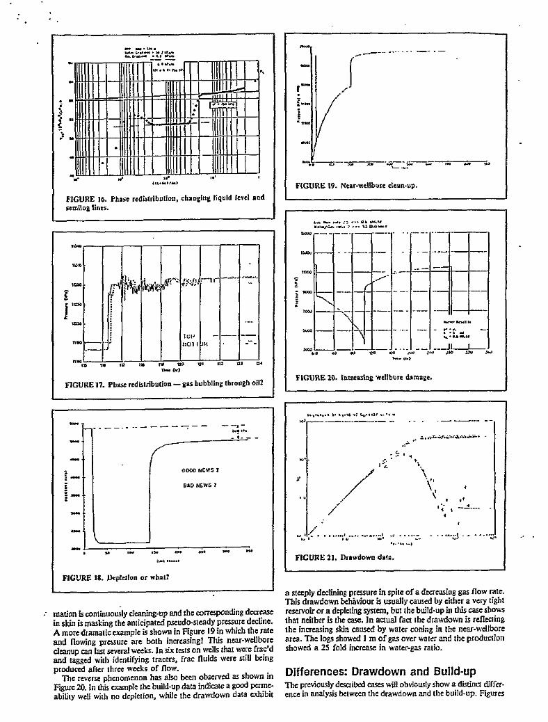
CHAPTER 3 DELIVERABILITY TESTS
1 INTRODUCTION
Deliverability tests have conventionally been called "back
pressure" tests because they make possible the prediction of well flow
rates against any particular pipeline "back pressure." Since most
flowing well tesks are performed to determine the deliverability of a
well, the term "deliverability tests" is used in this publication
rather than "back pressure tests." The purpose of these tests is to
predict the manner in which the flow rate will decline with reservoir
depletion.
The Absolute Open Flow (AOF) potential of a ~~11 is defined
as khe rate at which the well would produce against a zero sandface
back pressure. It cannot be measured directly but may be obtained from
deliverability kcsts. It is often used by regulatory authorities as a
guide in setting maximum allowable producing rates.
1.1 History
It iu interesting to note the historical development of
deliverability tests. In the early days, a well was tested by opening
it fully CO the atmosphere and measuring the gas flow rate, which was
termed the practical open flow pokential. This method ~8s recognized as
undesirable because khe pokential thus obtained depended on khe size of
the well tubing, and apart from the serious waskage of gas resulting
from such practices, wells were ofken damaged through water coning and
attrition by sand particles.
The basic work towards development of a practical test was
carried out by Pierce and Rawlins (1929) ,of the U.S. Bureau of Mines
and culminaked wikh the publication of the wel.l-known and widely used
Monograph 7 of Rzwlinu and Schellhardt (1936). Their kesk, known as the
3-1
3-2
"conventional back pressure test," consisted of flowing the well at
several different flow rates with each flow rate being continued to
pressure stabilization. They observed that a plot of the difference
between the square of the static reservoir pressure and the square of
the flowing sandface pressure versus the corresponding rate of flow
would yield a straight line on a logarithmic coordinate plot. They
showed that this stabilized deliverability plot could be empLoyed to
determine the well capacity at any flowing sandface presaute, including
zero, corresponding to absolute open flow conditions, and also showed
that it could be used to predict the behaviour of a well with reservoir
depletion.
The critical aspect of the Rawlins and Schellhardt conventional
deliverability test is that each separate flow rate must be continued
to stabilized conditions. In Low permeability reservoirs, the time
required to achieve pressure stabilization can be very large. As a
consequence the actual duration of flow while conducting conventional
tests on such reservoirs is sometimes not lengthy enough, and the
resulting data can be misleading. Cullender (1955) described the
"isochronal test" method which involves flowing the well at several
different flow rates for periods of equal duration, normally much less
than the time required for stabilization, with each flow period
commencing from essentially static conditions. A plot of such pressure
and flow rate data, as is described above for the conventional test,
gives a straight line or a transient deliverability plot. One flow rate
is extended to stabilization and a stabilized pressure-flow rate point
is plotted. A line through this stabilized point parallel to that
established by the isochronal points gives the desired stabilized
deliverability plot. This stabilized deliverability line is essentially
the same as that obtained by the conventional test.
Another type of isochtonal test was presented by Katz et al.
(1959, p. 448). This "modified iaochroiial test" has been used
extensively in industry. The modification requires that each shut-in
period between flow periods, rather than being long enough to attain
essentially static conditions, should be of the same duration as the
3-3
flow period. The actual unstabilized shut-in pressure is used for
calculating the difference in pressure squared for the nexr flow
point. Otherwise, the data plot is identical to that for an isochronal
test.
1.2 New Approach to Interpreting Gas Well Flow Tests
It is observed that there has been a progressively greater
saving of time, and a reduction in flared gas with the evolution of
various deliverability tests. Application of the theory of flow of
fluids through porous media, as developed in Chapter 2, results in a
greater understanding of the phenomena involved. Accordingly more
inFormation, and greater accuracy, can result from the proper conduct
and analysis of tests.
It will be shown in a later chapter that the analysis of data
from an isochronal type test, using the laminar-inertial-turbulent
(LIT) flow equation will yield considerable information concerning the
reservoir in addition to providing reliable deliverability data. This
may be achieved even without conducting the extended flow test which
is normally associated with the isochronal tests, thus saving still
more time and gas. For these reasons, the approach utilizing the LIT
flow analysis is introduced and its use in determining deliverability
is illustrated in this chapter. This will set the stage for subsequent
chapters where the LIT flow equation will be used fo determine certain
reservoir parameters.
2 FUNDAMENTAL EQUATIONS
The relevant theoretical considerations of Chapter 2 are
developed further in the Notes to this chapter to obtain the equations
applicable to deliverability tests. Two separate treatments with
varying degrees of approximation may be used to interpret the tests.
These will be called the "Simplified analysis" and the "LIT flow
analysis. "
3-4
2.1 Simplified Analysis
This approach is based on the well-known Monograph 7
(Rmulins and Schellhardt, 1936) which was the result of a Large number
of empirical observations. The relationship is co~~+~~nly expressed in
the form
q SC
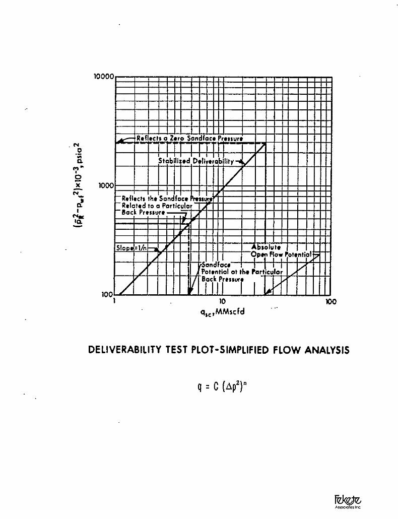
- c (p; - p$ 5 c(Ap')n (3-U
where
9 BC -. fl.ow rate at standard conditions, MMscfd
(14.65 psia, 60oF)
G = average reservoir pressure obtained by shut-in
of the well to complete stabilization, psia
= flowing sandface pressure, psia
3 = (pi - p:f)
c = a coefficient which describes the position of the
stabilized deliverability line
n = an exponent which describes the inverse of the slope
of the stabilized deliverability line.
It should be noted that pwf in the above equation is the
stabilized flowing sandface pressure resulting from the constant flow
rat=, q,,. If the pressure is not srabilized, C decreases with
duration of flaw but eventually becomes a fixed comcam at
stabilization. Time to stabilization and related matters is
discussed in detail in Section 7.1. In the Note$ to this chapter, it
is shown that n may vary from 1.0 for completely laminar flow in the
formation to 0.5 for fully turbulent flow, and it may thus be considered
to be a measure of the degree of turbulence. Usual.ly n will be between
1.0 and 0.5.
A plot of Ap* (= pi - pif) versus q,, on logarithmic
coordinates is a straight Line of slope i a6 shown in Figure 3-l.
Such a plot is used to obtain the deliverability potential of the well
against any sandface pressure, including the AOF, which is the
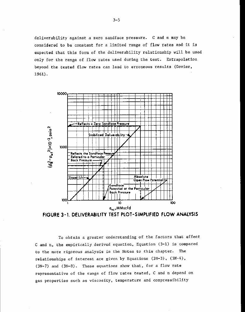
3-5
deliverability against a zero sandface pressure. C ad n may be
considered to be constant for a limited range of flow rates and, it is
expected that this form of the deliverability reLationship will be used
only for the range of flow rates used during the test. Extrapolation
beyond the tested flow raee~ can lead to erroneous results (Govier,
1961).
100 I IO 100
q,JAMscfd
FIGURE 3-1. DELIVERABILITY TEST PLOT-SIMPLIFIED FLOW ANALYSIS
To obta-ln a greater understanding of the Factors that affect
C and n, the empirically derived equation, Equation (3-l) is compared
to the more rigorous analysis in the Notes to this chapter. The
relationships of interest are given by Equations (3N-3), (3N-4),
(3N-7) and (3N-8). These equations show that, for a flow rate
representative of the rauge of flow rates tested, C and n depend on
gas properties such as viscosity, temperature and compressibility
3-6
factor, and reservoir properties such as permeability, net pay thickness,
external boundary radius, wellbore radius and well damage. As long as
these factors do not change appreciably, the same stabilized deliver-
ability plot should apply throughout the life of the well. In practice,
the viscosity, the compressibility factor of the gas and the condition
of the well may change during the producing Life of the well, and it is
advisable to check the values of C and n occasionally.
2.2 LIT Flow Analysis
Pressure-squared Approach
The utility of Equation (3-l), is Limited by its approximate
narure, The theory of flow developed in Chapter 2 and in the Notes to
this chapter confirms that the straight line plot of Figure 3-l is
really only an approximation applicable to the limited range of flow
rates tested. The true relationship if plotted on logarithmic
coordinates is a curve with an initial slope of i = 1.0 at very low
values of q,,, and an ultimate slope of i = 2.0 at very high values
of cl,,. Outside North America, there has been in general use a
quadratic form of the flow equation often called the Forchheimer or the
Houpeurt equation or sometimes called the turbulent flow equation. It
is actually the laminar-inertial-turbulent (LIT) flow equation of
Chapter 2, developed further in the Notes to this chapter, and is given
by Equation (3N-2)as
AP 2 E ;2 R - pif = a' qac + b' q& (3-2)
where
alqsc = pressure-squared drop due to laminar flow
and wellbore effects
b'q;c = pressure-squared drop due to intertial-turbulent
flow effects.
Equation (3-2) applies for all values of q,,. It is shown in
3-7
the Notes to this chapter that Equation (3-l) is only an approximation
of Equation (3-Z) for limited ranges of p,,.
In the derivation of Equation (3-21, an idealized situation
was assumed for the well and for the reservoir. It is important to
know the extent and the applicability of the assumptions,made when
test results are being interpreted. Sometimes anomalous results may be
explainable in terms of deviations from the idealized situations.
Accordingly, the assumptions which are clearly defined in Chapter 2,
Section 5.1 are summarized below:
1. Isothermal conditions prevail throughout the reservoir.
2. Gravitational effects are negligible.
3. The flowing fluid is single phase.
4. The medium Is homogeneous and isotropic, and the
porosity is constant.
5. Permeability is independent of pressure.
6. Fluid viscosity and compressibility factor are constant.
Compressibility and pressure gradients are small.
7. The radial-cylindrical flow model is applicable.
Pressure Approach
Since this approach is seldom used for the analysis of
deliverability tests, relevant equations have not been derived in the
Notes as was done for the pressure-squared approach. However, it can
be shown, by procedures similar, to those for the pressure-squared
approach, that
Ap Z sR - I 1 P,f = a q sc+b" 4zc (3-3)
where
a' 'qsc = pressure drop due to laminar flow and well effects
b"q' SC = pressure drop due to inertial-turbulent flow
effects
The application of Equation (3-3) is also restricted by the
assumptions listed for the pressure-squared approach.
3-8
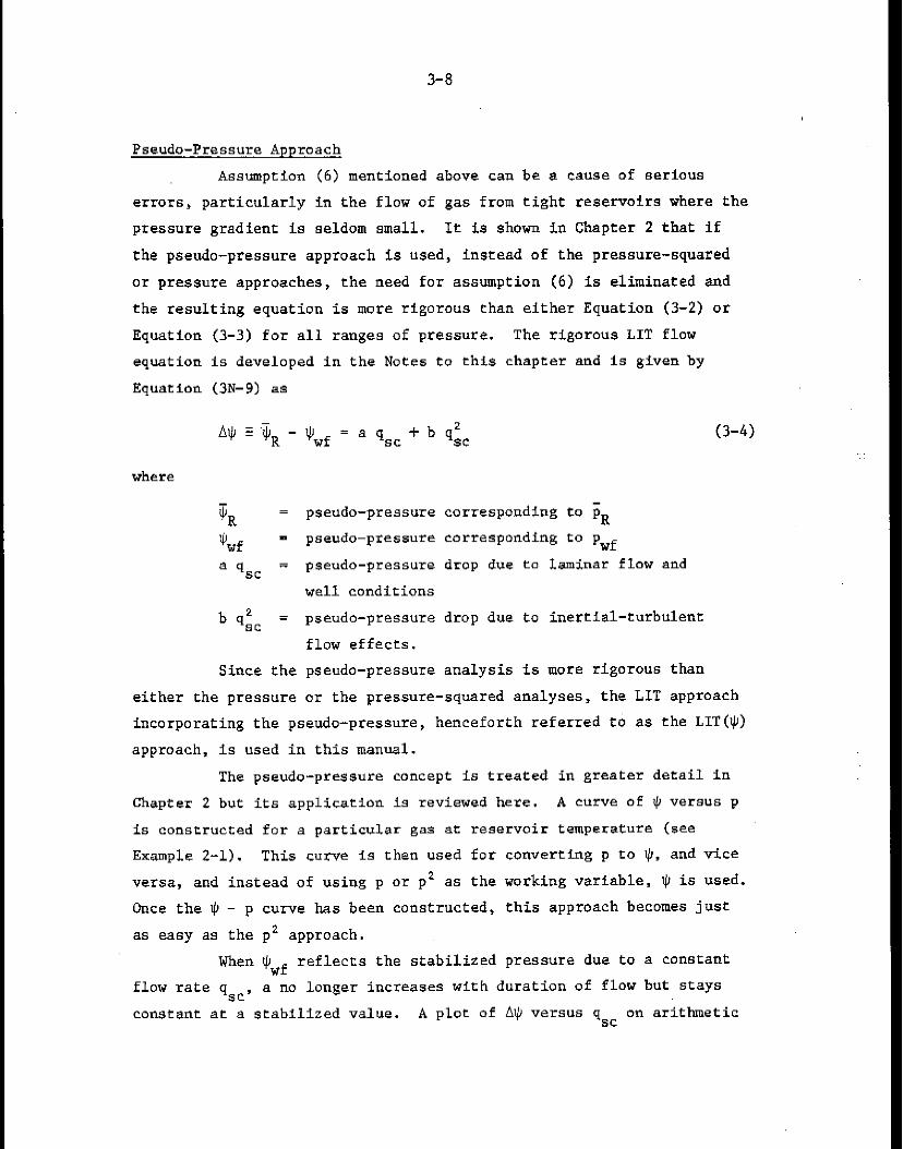
Pseudo-Pressure Approach
Assumption (6) mentioned above can be a cause of serious
enors, particularly in the flow of gas from tight reservoirs where the
pressure gradient is seldom small. It is shown in Chapter 2 that if
the pseudo-pressure approach is used, instead of the pressure-squared
or pressure approaches, the need for assumption (6) is eliminated and
the resulting equation is more rigorous than either Equation (3-2) or
Equation (3-3) for all ranges of pressure. The rigorous LIT flow
equation is developed in the Notes to this chapter and is given by
Equation (3N-9) as
4 q ‘$ - qwf = a qs, + b q2 SC
where
$R = pseudo-pressure corresponding to sR
Ilr wf = pseudo-pressure corresponding to pwf
a 4sc = pseudo-pressure drop due to leminar flow and
well conditions
b q2 SC = pseudo-pressure drop due to inertial-turbulent
flow effects.
Since the pseudo-pressure analysis is more rigorous than
either the pressure or the pressure-squared analyses, the LIT approach
incorporating the pseudo-pressure, henceforth referred to as the LIT(q)
approach, is used in this manuel.
The pseudo-pressure concept is treated in greater detail in
Chapter 2 but its application Is reviewed here. A curve of I/J versus p
is constructed for a particular gas at reservoir temperature (see
Example 2-l). This curve is then used for converting p to q, and vice
versa, and instead of using p or p2 as the working variable, 9 is used.
Once the $ - p curve has been constructed, this approach becomes just
as easy as the p2 approach.
When Qwf reflects the stabilized pressure due to a constant
flow rate q,,. a no Longer increases with duration of flow but stays
constant at a stabilized value. A plot of A@ versus q,, on arithmetic
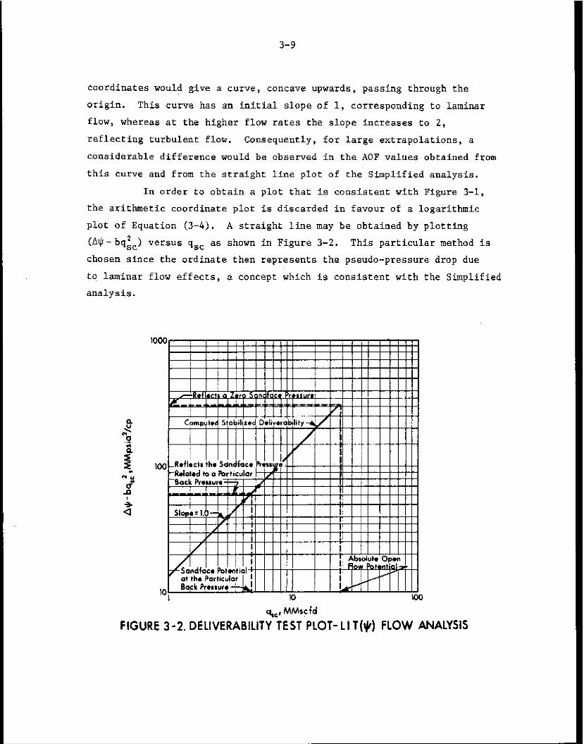
3-9
coordinates would give a curve, concave upwards, passing through the
0rigii-l. This CUFV~ has an initial slope of 1, cor,resposding to laminar
flow, whereas at the higher fl.ow rates the slope increases to 2,
reflecting turbulent flow. Consequently, for large extrapolations, a
considerable difference would be obsened in the AOF values obtained from
this curve and from the straight line plot of the Simplified analysis.
In order to obtain a plot that ia consistent with Figure 3-1,
the arithmetic coordinate plot is discarded in favour of a logarithmic
plot of Equation (3-4). A straight line may be obtained by plotting
(A$ - bq;,) Y~TSUG g,, as shown in Figure 3-2. This particular method is
chosen since the ordinate then represents the pseudo-pressure drop due
to laminar flow effects, a concept which iu consistent with the Simplified
q,,, MMscfd
FIGURE 3-2. DELlVERABlLlTY TEST PLOT-LIT(q) FLOW ANALYSIS
3-K
The deliverability potential of a well against any sandface
pressure may be obtained by solving the quadratic Equation (3-4) for the
particular value of A9
q = -a + J(a2 -c 4 b A$)
SC 2b (3-5)
a and b in the LIT($) flow analysis depend on the same gas 'and
reservoir properties as do C and n in the Simplified analysis except for
viscosity and compressibility factor. These two variables have been
taken into account in the conversion of p to @, and consequently, will
not affect the deliverability relationship constants a and b.. It
EOllOWS, therefore, that the stabilized deliverability Equation (3-41,
or its graphical representation, is more likely to be applicable
throughout the life of a reservoir than Equations (3-l), (3-2) or (3-3).
3 DETERMINATION OF STABILIZED FLOW CONSTANTS
Deliverability tests have to be conducted on wells to
determine, among other things, the values of the stabilized flow
constants. Several techniques are available to evaluate C and n, of
the Simplified analysis, and a and b, of the LIT($) flow analysis,
from deLiverability data.
3.1 Simplified Analysis
A logarithmic coordinate pl.ot of Ap' venus qs, should yield
a straight line over the range of flow rates tested. The slope of this
stabilized deliverability line gives $ from which n can be calculated.
The coefficient C in Equation (3-l) is then obtained from
(3-6)
3-11
3.2 LIT($) Flow Analysis
Least Squares Method
A plot of (A$-b&) versus q,,, on logarithmic coordinates,
should give the stabilized deliverability line. a and b may be obtained
from the equations given below (Kulczycki, 1955) which are derived by
the curve fitting method of least squares
(3-7)
(3-8)
where
N = number of data points
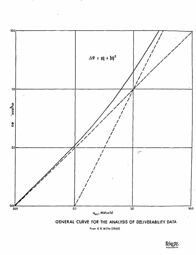
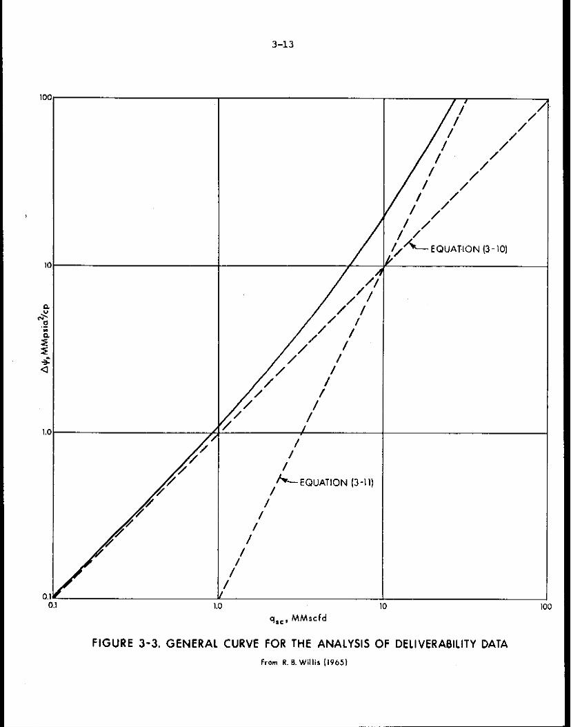
Graphical Method
This method utilizes the "general curve," developed by Willis
(1965), shown in Figure 3-3. Before discussion on the use of the
general curve method, the details of its development should be clearly
understood.
Equation (3-4), with a = b = 1 can be written as
A$ = qsc + 4’ 9c O-9)
The straight 11neu in Figure 3-3, which is a logarithmic coordinate
plot of A$ versus q, are represented by the equations
A+ = q SC (3-10)
(3-11)
3-12
If the plots of Equations (3-10) and (3-11) are added for the same
value of q SC'
the resulting plot is the general curve.
To distinguish Figure 3-3 from a data plot, the latter will
be referred to as the deliverability plot.
To determine a and b, actual data are plotted on logarithmic
coordinates of the same size as Figure 3-3. This stabilized
deliverability data plot is laid upon the general curva plot, and
keeping the axes of the two plots parallel, a position is found where
the general curve best fits the points on the data plot. The stabilized
deliverability curve is now a trace of the general curve. The value of
a is read directly as A$ for the point on the deliverability plot where
the line given by Equation (3-10) intersects the line qac = 1 of the
dellverability plot. The value of b is read directly as A$ for the
point on the deliverability plot where the line given by Equation (3-11)
intersects the line p SC = 1 of the deliverability plot,
If the point at which'a*is to be read does not intersect the
P SC = 1 line of the deliverability plot, 'a"may instead be read where
q sc equals 10 or 100 and must then be divided by 10 or 100, respectively,
to get the correct value. Similarly, b may be read where q,, equals 10
or 100 and must then be divided by 10' or loo*, respectively.
The advantage of this method is the speed with which
deliverability data can be analyzed. However, it should be used only
when reliable data are available.
The above procedure may be applied to data from a conventional
test to yield a stabilized deliverability curve. With isochronal data,
however, it will yield a transient deliverability curve. To obtain the
stabilized deliverability curve, it should be remembered that the value
of b is independent of duration of flow and must be the same for the
stabilized and the transient deliverability relationships. Accordingly,
the general curve is positioned so that it passes through the stabilized
flow point and maintains the value of b obtained from the transient
deliverability curve.
The application of this graphical method to calculate a and b
is illustrated by Example 3-4 in Section 4.3.
3-13
101
/ LEQUATION (3-11)
g,,, MMscfd 100
FIGURE 3-3. GENERAL CURVE FOR THE ANALYSIS OF DELIVERABILITY DATA
From R. 8. Willil (19451
3-14
The general curve of Figure 3-3 may also be used with the
LIT(p') approach. The method is the same as described above except
Equation (3-2) is now fit instead of Equation (3-4).
4 TESTS INVOLVING STABILIZED FLOW
In the preceding analyses, C or a are constant only when
stabilization has been reached. Before stabilization is achieved, the
flow is said to be transient. Tests to determine the stabilized
deliverability of a well may combine both transient and stabilized
conditions. Various tests that may be used directly to obtain the
deliverability or the AOF of a well are described in this section along
with examples of their Interpretation by both the Simplified and the
LIT($) flow analyses. General guidelines for the field conduct and
reporting of these tests are discussed in a later chapter. All the
tests treated in this section have at least one, and sometimes all, of
the flow rates run until pressure stabilization is achieved. This is
very important as, otherwise, the deliverability obtained will not
reflect stabilized conditions and will thus be incorrect. Tests in
which no one flow race is extended to stabilized conditions will be
discussed in Section 5.
4.1 Conventional Test
As mentioned in Section 1, Pierce and Rawlins (1929) were the
first to propose and set out a method for testing gas wells by gauging
the ability of the well to flow against various back pressures. This
type of flow test has usually been designated the "conventional"
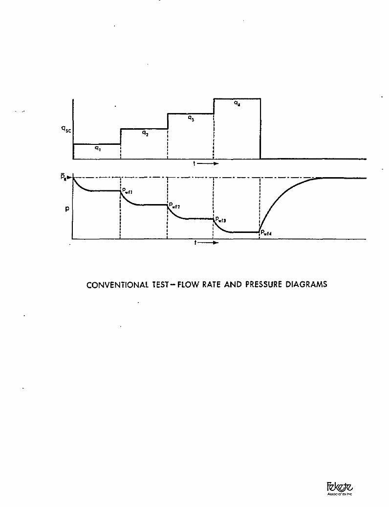
deliverability test. TO perform a conventionaL test, the stabilized
shut-in reservoir pressure, p,, is determined. A flow rate, qsc, is
then selected and the well is flowed to stabilization. The stabilized
flowing pressure, p,f, is recorded. The flow rate is changed three or
four times and every time the well is flowed to pressure stabilization.
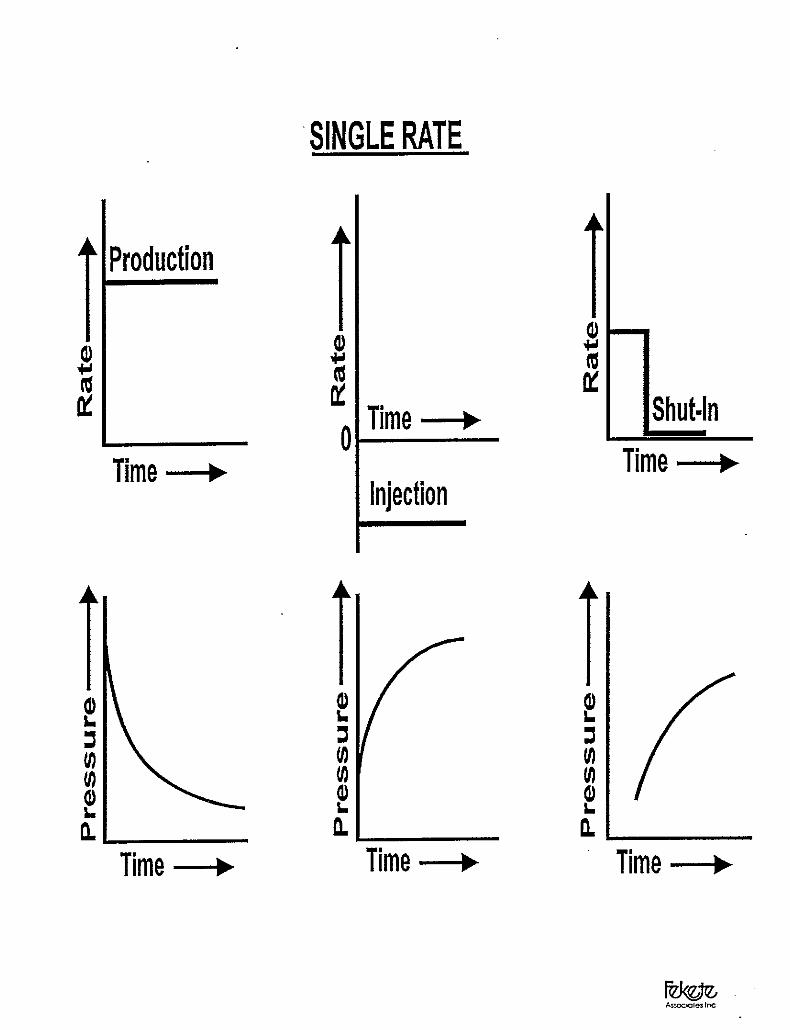
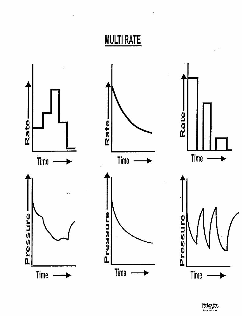
The flow-rate and pressure histories for such a test are depicted in
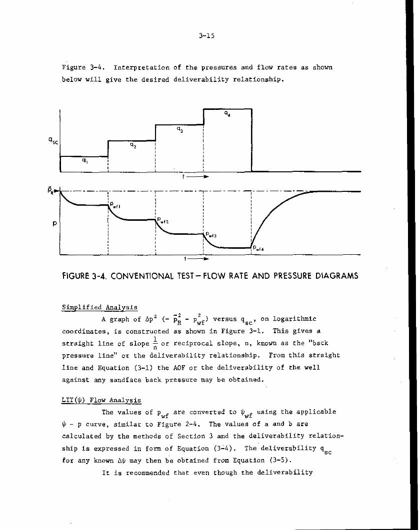
3-15
Figure 3-4. Interpretation of the pressures and flow rates as shown
below will give the desired deliverability relationship.
----7.------ 7-----l-.--
P
t-
FIGURE 3-4. CONVENTIONAL TEST- FLOW RATE AND PRESSURE DIAGRAMS
Simplified Analysis
A graph of bp* (= ;; - p;f) versus qsc, on logarithmic
coordinates, is constructed a~ shown in Figure 3-1. This gives a
straight line of slope i or reciprocal slope, n, known as the "back
pressure line" or the deliverability relationship. From this straight
line and Equation (3-l) the AOF or the deliverability of the well
against any sandface back pressure may be obtained.
LIT($) Flow Analysis
The values of pwf are converted to Q,, using the applicable
$ - p curve, similar to Figure 2-4. The values of a and b are
calculated by the methods of Section 3 and the deliverability relation-
ship is expressed in form of Equation (3-4). The deliverability q,,
for any known A$ may then be obtained from Equation (3-S).
It is recommended that even though the deliverability

3-16
relationship is derived by computation, the equation obtained should be
plotted on logarithmic coordinates along with the data points. Data
which contain significant errors will then show up easily. ErrOIleOUS
data points must be discarded and the deliverability relationship then
recalculated.
A sample deliverability calculation for a conventional test by
both the Simplified and the LIT($) flow analyses is shown In Example 3-l
(for gss composition see Example A-l; for the Q - p curve see Figure 2-4).
Although in many instances, both the Simplified and LIT(@)
flow analyses will give the same reuult, extrapolation by the Simplified
analysis beyond the range of flow rates tested can cause significant
errors. Such il situation is well illustrated by the calculations for a
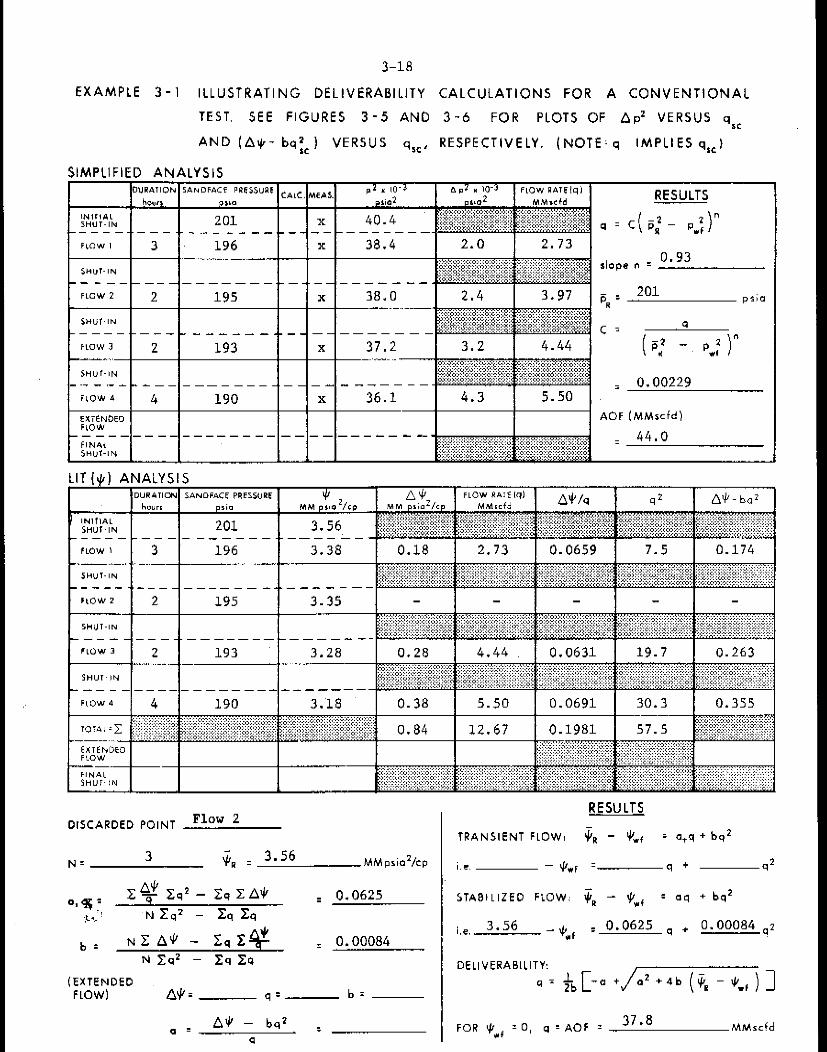
conventional Cest (Example 3-l). The LIT($) flow analysis gives an AOF
of 37.8 MMscfd while the Simplified analysis yields an AOF of 44.0 MMscfd.
This method of testing and the interpretation of the data iu
relatively simple, and the method has been considered the basic
acceptable standard fur testing gas wells for many years.
In a reservoir of very high permeability, the time required
to obtain stabilized flow fates and flowing pressures, as well as a
stabilized shut-in formation pressure is usually not excessive. In
this type of reservoir a properly stabilized conventional deliverability
test may be conducted in a reasonable period of time. On the other
hand, in low permeability reservoirs the time required to even
approximate stabilized flow conditions may be very long. In this
situation, It IS not practical to conduct a completely stabilized test,
and since the results of an unstabilized test can be very misleading,
other methods of testing should be used to predict well behaviour.
4.2 Isochronal Test
The conventional delivetsbilLcy test carried out under
stabilized conditions, qualifies as an acceptabLe approach to attslning
the relationship which is essential to the proper interpretation of
tests, because it extends each flow rate over a period of time
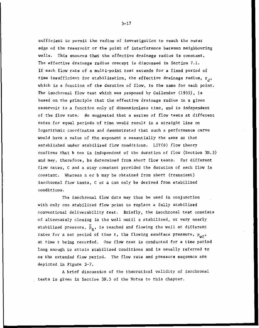
3-17
sufficient to permit the radius of investigation to reach the outer
edge of the reservoir or the point of interference between neighbouring
wells. This ensures that the effective drainage radius is constant.
The effective dralnage radius concept is discussed in Section 7.1.
If each fl.ow rate of a multi-point test extends for a fixed periad of
time insufficient for stabilization, the effective drainage radius, td,
which is a function of the duration of flow, is the same for each point.
The isochronal flow test which was proposed by Cullender (1955), is
based on the principle that the effective draInage radius in a given
reservoir is a function only of dimensionless time, and is independent
of the flow i-ate. He suggested that a series of flow tests at different
rates for equal periods of time would result in a straight line on
logarithmic coordinates and demonstrated that such a performance curve
would have a value of the exponent n essentially the same as that
established under stabilized flow conditions. LIT($) flow theory
confirms that b too is independent of the duration of flow (Section 3N.3)
and may, therefore, be determined from short flow tests. For different
flow rates, c and a stay constaflt provided the duration of each flow is
constant 1 Whereas n or b may be obtained from short (transient)
isochronal flow tests, C or a can only be derived from stabilized
conditions.
The isochronal flow data may thus be used in conjunction
with only one stabilized flow point to replace a fully stabilized
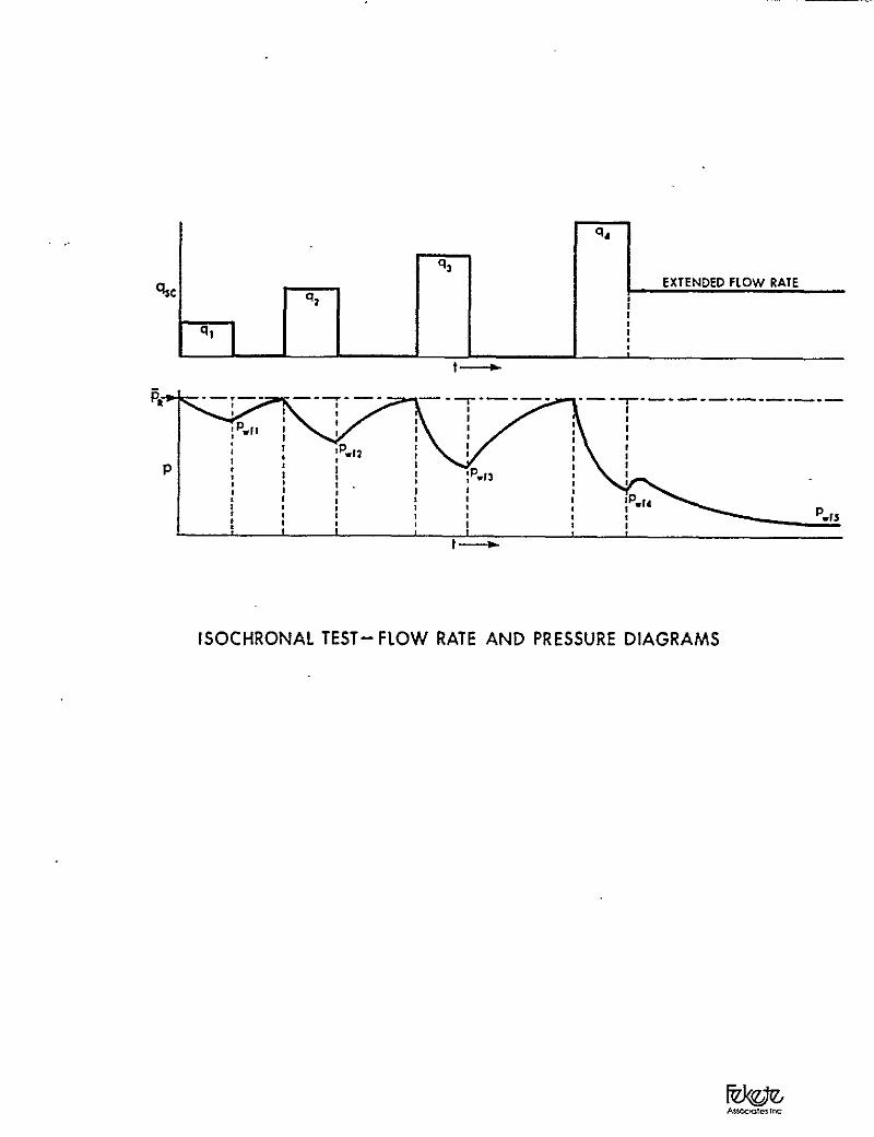
conventional deliverability test. Briefly, the isochronal test consists
of alternately closing in the well until a stabilized, or very nearly
stabilized pressure, &, is reached and flowing the well at different
rates for a set period of time t, the flowing sandface pressure, pwf,
at time c being recorded. One flow test is conducted for a time period
long enough to atrain stabilized conditions and is usually referred CO
as the extended flow period. The flow rate and pressure sequence are
depicted in Figure 3-7.
A brief discussion of the theoretical validity of isochronal
tests is given in Section 3N.5 of the Notes to this chapter.
3-18
EXAMPLE 3-1 ILLUSTRATING DELlVERAi3lllTY CALCULATIONS FOR A CONVENTIONAL
TEST. SEE FIGURES 3-5 AND 3-6 FOR PLOTS OF Ap’ VERSUS q SC
AND (A*- bqtt) VERSUS q,,, RESPECTIVELY. (NOTE: q IMPLIES q,,)
“. _.,-.̂ ,.., -
SH”f-lN .̂ --,_-- ----------------------- ? 0.00229
FLOW 4 4 190 x 36.1 4.3 5.50 AOF l~tkcfd~
DISCARDED POINT FLow ’ RESULTS
TRANSIENT FLOW! ii - k‘ = a+q + bq2
I.C. -kt z 4 + q*
STABILIZED FLOW: GR - qw+ : aq + b$
i.e. 3’56 - $I rf : 0.0625 q + 0.00084 q~
DELIVERABILITY:
q = ib[-a + /++4b (Ir, -J;,)]
FOR vJ*‘ zD, qEAOF I 37.8 MMrcfd
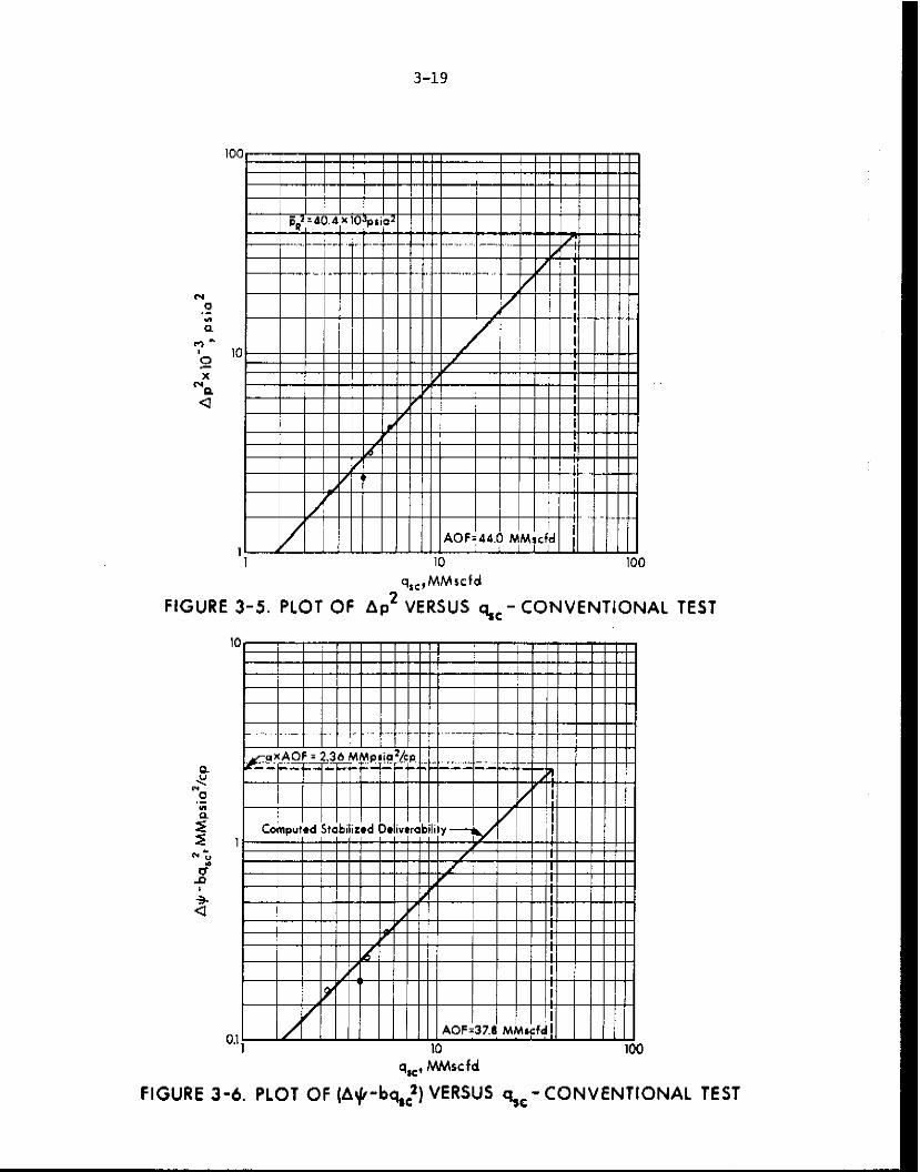
3-19
q,,,MM,cfd
FIGURE 3-5. PLOT OF Ap2 VERSUS q,, - CONVENTIONAL TES IT
FIGURE 3-6. PLOT OF (A*-bq:) VERSUS q,c- CONVENTIONAL TEST
3-20
t-
.
7 EXTENDED FLOW RATE
I
1
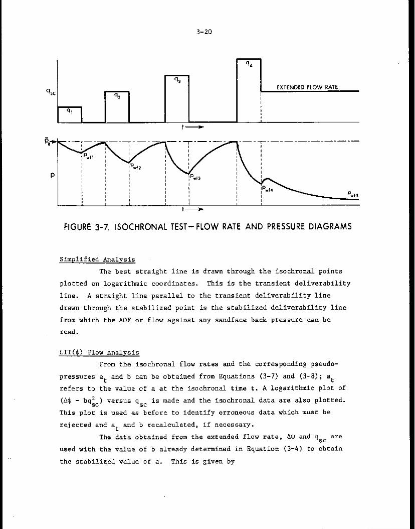
FIGURE 3-7. ISOCHRONAL TEST- FLOW RATE AND PRESSURE DIAGRAMS
Simplified Analysis
The best straight line is drawn through the isochronal points
plotted on logarithmic coordinates. This is the transient deliverability
line. A straight line parallel to the transient deliverability line
drawn through the stabilized point is the stabilized deliverability line
from which the AOF or flow against any sandface back pressure can be
read.
LIT($) Flow Analysis
From the isochronal flow rates and the corresponding pseudo-
pressures at and b can be obtained from Equations (3-7) and (3-8); at
refers to the value of a at the isochronal time t. A logarithmic plot of
(A$ - bq;J versus qgc is made and the isochronal data are also plotted.
This plot is used as before to identify erroneous data which must be
rejected and a t and b recalculated, if necessary.
The data obtained from the extended flow rate, 4$ and qsc are
used with the value of b already determined in Equation (3-4) to obtain
the stabilized value of a. This is given by
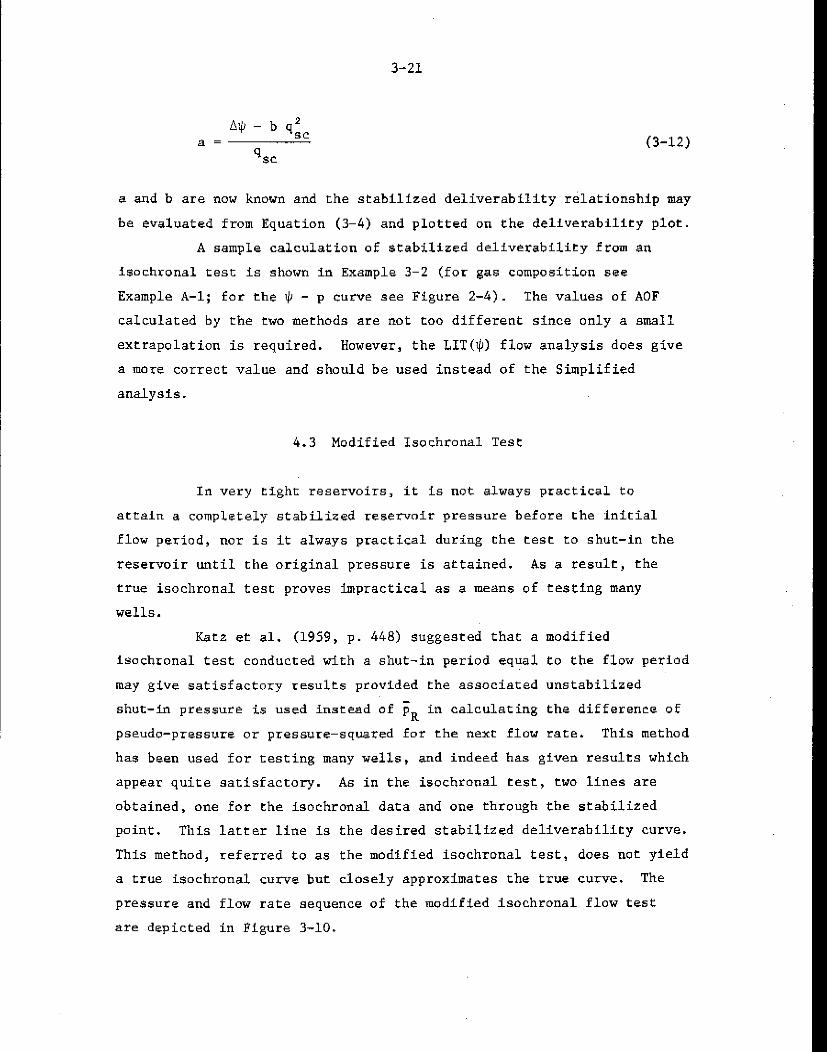
3-21
(3-12)
a and b are now known and the stabilized deliverability relationship may
be evaluated from Equation (3-4) and plotted on the deliverability plot.
A sample calculation of stabilized deliverability from an
isochronal fest is shown in Example 3-2 (for gas composition see
Example A-l; for the $ - p curve see Figure 2-4). The values of AOF
calculated by rhe twcl methods are not too different since only a small
extrapolation is required. However, the LIT($) flow analysis does give
a more correct value and should be used instead of the Simplified
analysis.
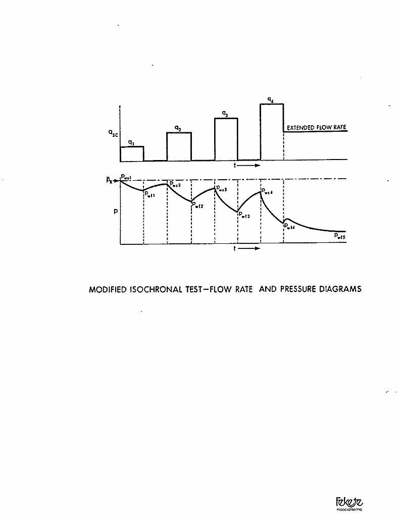
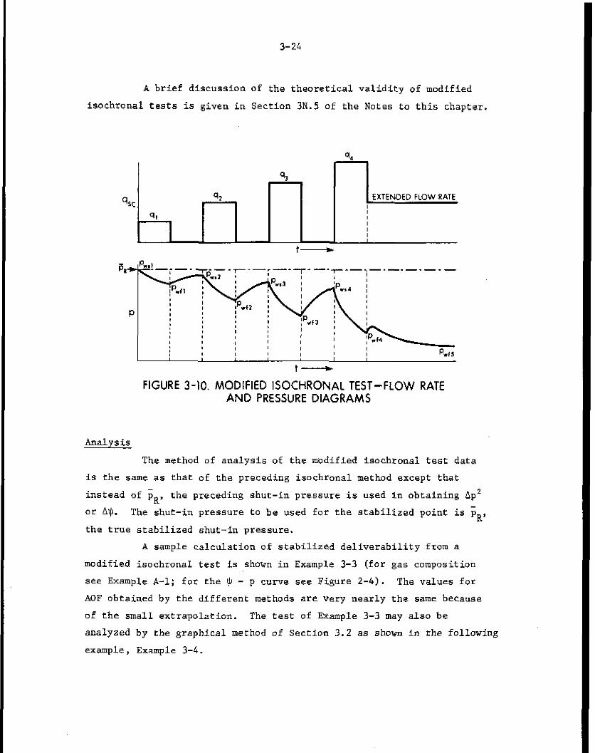
4.3 Modified Isochronal Test
In very tight reservoirs, it is not always practical to
attain a completely stabilized reservoir pressure before the initial
flow period, nor is it always practical during the test to shut-in the
reservoir until the original pressure is attained. Aa a result, the
true isochronal test proves impractical as a means of testing many
wells.
Katz et al, (1959, p. 448) suggested that a modified
isochronal test conducted with a shut-in period equal to the flow period
may give satisfactory results provided the associated unstabilized
shut-in pressure is used instead of pR in calculating the difference of
pseudo-pressure or pressure-squared for the next flow rate. This method
has been used for testing many wells, and indeed has given results which
appear quite satisfactory. As in the isochrdnal test, two lines are
obtained, one for the isochronal data and one through the stabilized
point. This latter line 1s the desired stabilized deliverability curve.
This method, referred to as the modified isochronal test, does not yield
a true isochronal curve but closely approximates the true curve. The
pressure and flow rate sequence of the modified isochronal flow test
are depicted in Figure 3-10.
3-22
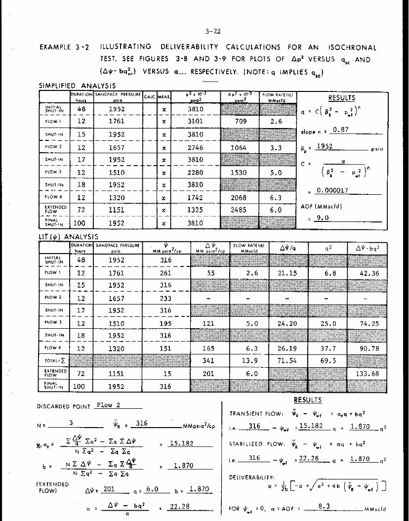
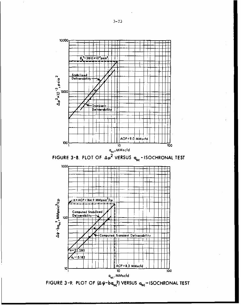
EXAMPLE 3 -2 ILLUSTRATING DELIVERABILITY CALCULATION5 FOR AN ISOCHRONAL
TEST. SEE FIGURES 3-8 AND 3,-9 FOR PLOTS OF Apz VERSUS clsc AND
I&- baf,) VERSUS Q... RESPECTIVELY. (NOTE: q IMPLIES q,,)
SIMPLIFIED ANALY
RESULTS
q _ c p @z _ p,; ( )”
k * *I I 1952 x 3810
i 0.000017 I.320 x 1742
DISCARDED POINT Flow 2
0 = A'# - bq* : 22.28 9
RESULTS
TRANSIENT FLOW! 4, - Q : +g * bq2
1.e. 316 - $w.r zL5.182 q .+ 1.870 qz
STABILIZED FLOW; qR - qwf : eq + bq2
I.e. 316 uuqwt z22.28 q + 1.870 qz
DEL'VERAB'L'~~~ +b Cm0 +& + *b ('JR - ew, ) ]
FOR $w‘ = 0, q = AOF : 8.3 MMrcfd
3-x
!
I I I I
I
AOF: 9.0 MM,cfd loo 1 II/l
1 10 100
q,<,MMscfd
FIGURE 3-8. PLOT OF Ap2 VERSUS q,, - ISOCHRONAL
q=, MMscfd
GURE 3-9. PLOT OF (At/t-bq,:) VERSUS q,,-ISOCHRON
3-24
A brief discussion of the theoretical validity of modified
lsochronal tests is given in Section 3N.5 of the Notes to this chapter.
92 EXTENDED FLOW RATE
P
Analysis
t-
t---w FIGURE 3-10. MODIFIED ISOCHRONAL TEST-FLOW RATE
AND PRESSURE DIAGRAMS
The method of analysis of the modified isochronal test data
is the came es that of the preceding isochronal method except that
instead of &, the preceding shut-in pressure is used In bbtainfng ap2
or A$. The shut-in pressure to be used for the stabilized point is p,,
the true stabilized shut-in pressure.
A sample calculation of stabilized deliverability from a
modified isochronal test is shown in Example 3-3 (for gas composition
see Example A-l; for the I) - p curve eee Figure 2-4). The values for
ilDF obtained by the different methods are very nearly the eeme because
of the small extrapolation. The test of Example 3-3 may also be
analyzed by the graphical method of Section 3.2 as shown in the following
example, Example 3-4.
3-25
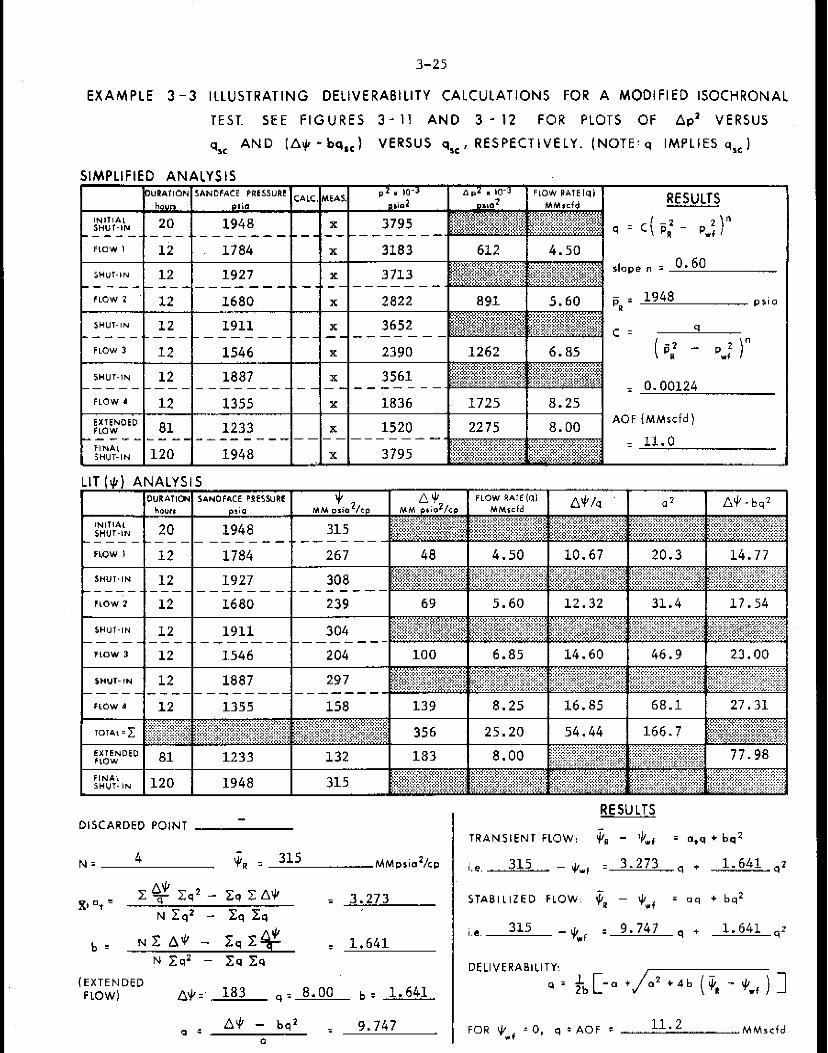
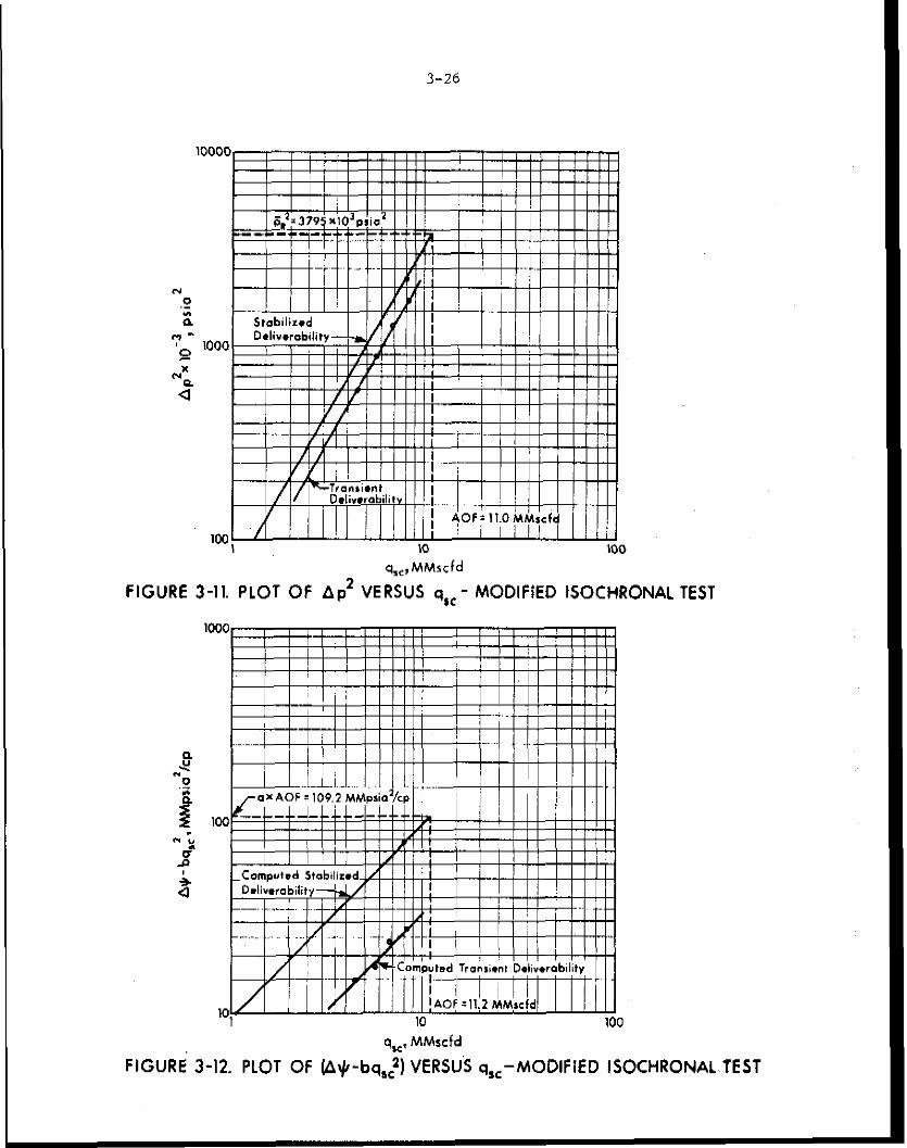
EXAMPLE 3-3 ILLUSTRATING DELlVERAElllTY CALCULATIONS FOR A MODIFIED ISOCHRONAL
TEST. SEE FIGURES 3-11 AND 3 - 12 FOR PLOTS OF Ap’ VERSUS
qsc AND IA9 -h,c) VERSUS q,,. RESPECTIVELY. (NOTE:~ IMPLIES 4,<)
SIMPLIFIED ANAlYSIS
LIT ($) ANALYSIS
DISCARDED POINT
N= 4 <, = 315 MMpri&p
(EXTENDED FLOWI A+;~, 183 q' 8.00 b: 1.641
0 - A'# - bq2 = 9.747
0
RESULTS
TRANSIENT FLOW: & - lr;, = a,q + bqZ
i.e. 315 - h z 3.273 q + -LAG_ qz
STA81tlZED FLOW: $ - $v;r = oq + bqz
1.d. 315 -J;{ : 9.747 q + 1.641 qz
DELIVERABIIITY:
q = ib[-” t /a2 +4b ($ - VJ”,) 1
FOR qwf -0, q :AOF - 11.2 MMrcfd
3-26
FIGURE 3-11. PLOT OF &I’ VERSUS q,,- MODIFIED ISOCHRONAL
+,MMscfd
q,,, MMscfd
FIGURE 3-12. PLOT OF (A$-bq,:) VERSUi q,, -MODlF IED ISOCHRONAL~~TEST
3-27
EXAMPLE 3-4
Introduction This,example illustrates the application of the graphical
method of Section 3-2 to the analysis of modified isochronal test data.
Problem Calculate the values of a, b and AOF for the modified
isochronal test data of Example 3-3.
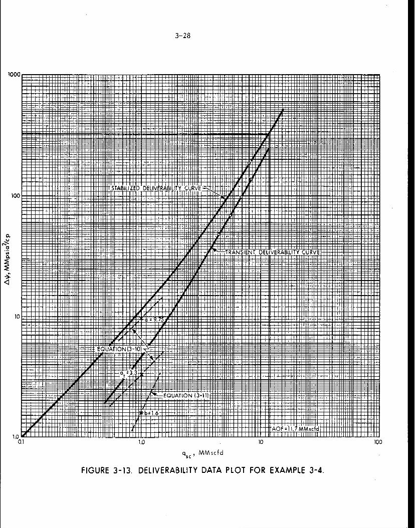
So,lution Plot A$ versus qsc (transient, modified isochronal data) on
3x3 logarithmic coordinates of the same size as the general curve of
Figure 3-3. This deliverability data plot is shown in Figure 3-13:
The transient deliverability curve is drawn from the best
match of the deliverability data plot and the general curve. The values
of a and b are obtained from the intersections of the straight lines,
repr:sented by Equations (3-10) and (3-U), with the q = 1 line of SC
the deliverability data plot. This gives
at = 3.3
b = 1.6
Plot the stabilized flow point and maintaining the value of
b = 1.6 draw the stabilized deliverability curve. The intersection of
the straight line, represented by Equation (3-lo), with the q,, = 1 line
of the deliverability data plot gives
a = 9.75
and the resulting deliverability curve shows an
AOF = 11.7 MMscfd
DiSCUSSiOIl Figure 3-3 may be used to obtain good approximations for
a, b, and AOF, but it is recommended that the calculation methods of
Examples 3-1, 3-2 and 3-3 using the LIT($,) flow analysis be used Ear
better results.
3-28
3-29
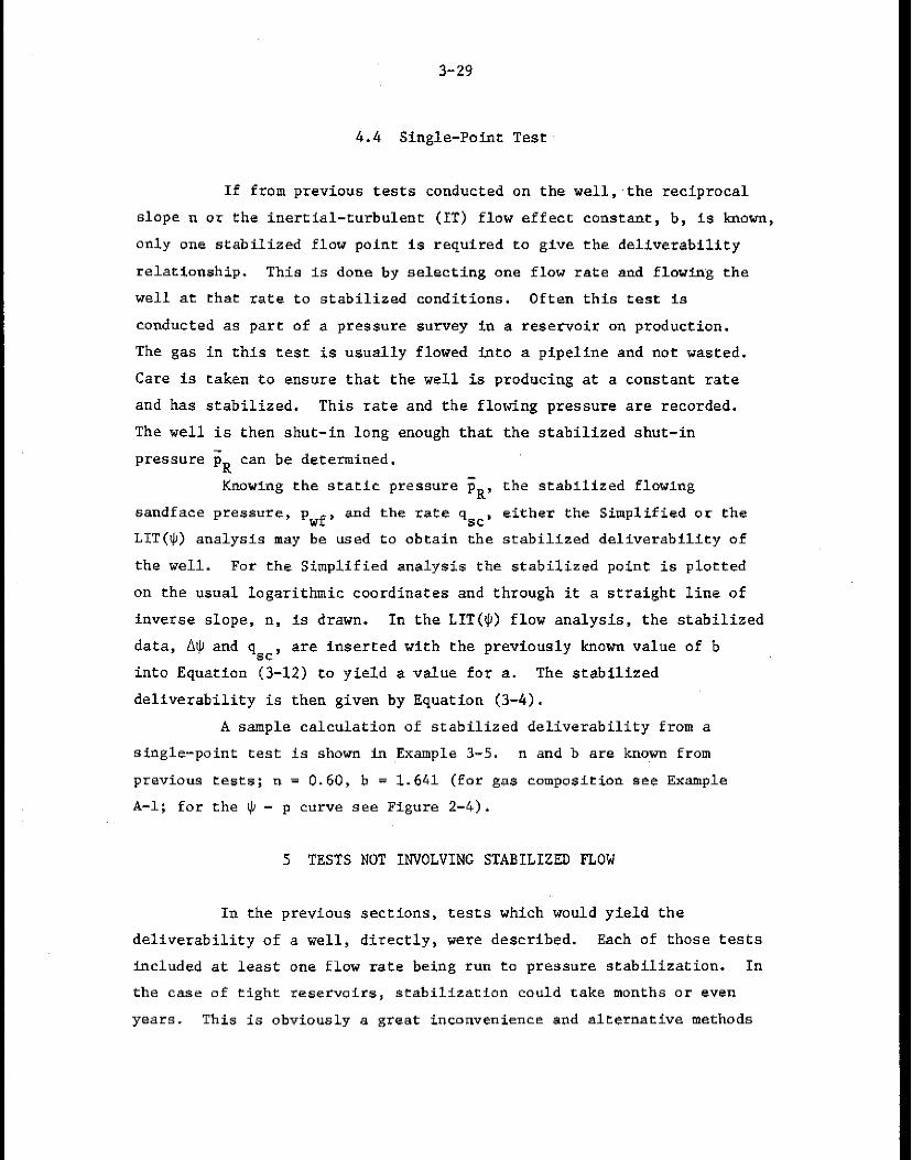
4.4 Single-Point Test
If from previous tests conducted on the well,,the reciprocal
slope n or the inertial-turbulent (IT) flow effect constant, b, is howa,
only one stabilized flow point is required CO give the deliverability
relatXonship. This is done by selecting one flow rate and flowing the
well at that tate to stabilized conditions. Often this fest is
conducted as part of a pressure survey 1n a reservoir on production.
The gas in this test is usually flowed into a pipeline and not wasted.
Care is taken to ensure that the well is producing at a constant rate
and has stabilized. This rate and the flowing pressure are recorded.
The well is then shut-in long enough that the stabilized shut-in
pressure GR can be determined.
Knowing the static pressure p,, the stabilized flowing
sandface pressure, pwf, and the rate q,,, either the Simplified or the
LIT($) analysis may be used to obtain the srabilized deliverability of
the well. For the Simplified analysis the stabilized point is plotted
on the usual logarithmic coordinates and through it a straight line of
inverse slope, n, is drawn. In the LIT($) flow analysis, the stabilized
data, AIJJ and q SC
are inserted with the previously known value of b
into Equation (3-12) to yield a value for a. The stabilized
deliverability is then given by Equation (3-4).
A sample calculation of stabilized deliverability from a
single-point test is shown in Example 3-5. n and b are known from
previous tests; n = 0.60, h = 1.641 (for gas composition see Example
A-l; for the IJ - p c"r"e see Figure 2-4).
5 TESTS NOT INVOLVING STABILIZED FLOW
In the previous sections, tests which would yield the
deliverability of a well, directly, we're described. Each of those tests
included at least one flow rate being rm to pressure stabilization. In
the case of tight reservoirs, stabilization could take months or even
ye&Y. This is obviously a great inconvenience and alternative methods
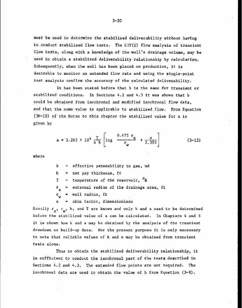
3-30
must be used to determine the stabilized deliverability without having
to conduct stabilized flow tests. The LIT($) flow analysis of transient
flow teats, along with a knowledge of the well’s drainage volume, may be
used to obtain a stabilized deliverability relationship by calculation.
Subsequently, when the well has been placed on production, it is
desirable to monitor an extended flow rate and using the single-point
test analysis confirm the accuracy of the calculated deliverability.
It has been stated before that b is the same for transient or
stabilized conditions. In Sections 4.2 and 4.3 it was shown that b
could be obtained from isochronal and modified isochronal flow data,
and that the same value is applicable to stabilized flow. From Equation
(3N-10) of the Notes to this chapter the stabilized value for a is
given by
T a = 3.263 x lo6 n
0.472 re rw
+* I
(3-13)
where
k = effective permeability to gas, md
h = net pay thickness, ft
T = temperature of the reservoir, OR
r - e external radius of the drainage area, ft
r = w well radius, ft
s = skin factor, dimensionless
usu;llly re, rw, 11, and T are know0 and onSy k and s need to be determined
before the stabilized value of a can be calculated. In Chapters 4 and 5
it is shown how k and a may be obtained by the analysis of the transient
drawdown or build-up data. For the present purpose it is only necessary
to note that reliable values of k and s may be obtained from transient
tests alone.
Thus to obtain the stabilized deliverability relationship, it
is sufficient to conduct the isochxonal part of the tests described in
Sections 4.2 and 4.3. The extended flow points are not required. The
isochronal data are used to obtain the value of b from Equation (3-8).
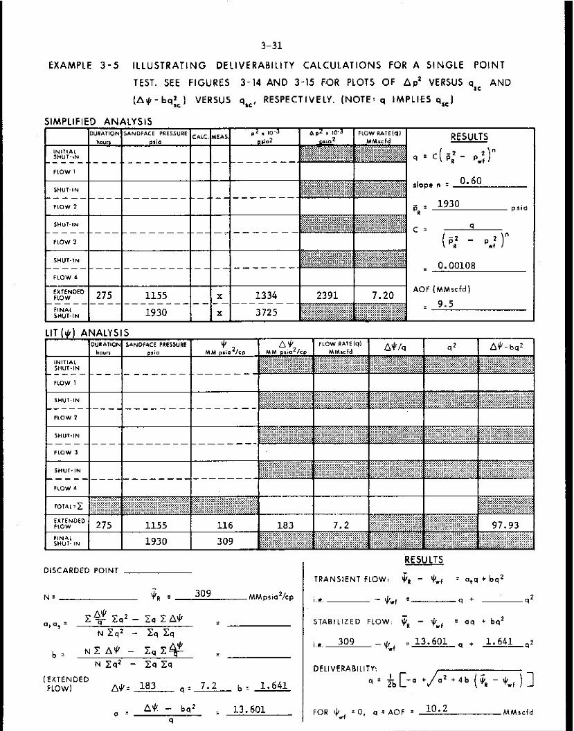
EXAMPLE 3-s ILLUSTRATING DELIVERABILITY CALCULATIONS FOR A SINGLE POINT
TEST. SEE FIGURES 3-14 AND 3-15 F,OR PLOTS Of Ap* VERSUS q,, AND
b-b- ha:,) VERSUS qsc, RESPECTIVELY. (NOTE: q IMPLIES q,,)
RFSIJITS
i 0.00108
AOF (MMrcfd)
= 9.5
DISCARDED POINT
b= NIXA'!-- ZqZ '+' _ N Es2 - Eq Zq
[EXTENDED FLOW1 A+: 183 q' 7.2 br 1.641
0 z A'k - bql i 13.601
9
RESULTS
TRANSIENT FLOW! JR - qwf = +q + bq2
1.e. -hYt = 9 + qz
STABILIZED FLOW: T@ - qwc;, : aq + bq*
I.#. 309 -e,, 113.601 q + 1.641 qz
DELIVERABILITV:
q : tb[-O + b2+4b (qn -J;,)]
FOR $*# -4, q’AoF ? 10.2 MMscfd
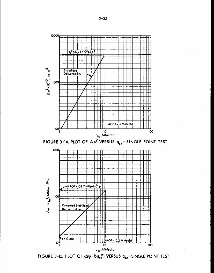
3-32
10000
FIGURE 3-14. PLOT OF Ap2 VERSUS q,< - SINGLE POINT TEST
FIGURE 3-15. PLOT OF (A+bq$ VERSUS &-SINGLE POIN T TEST
3-33
The value of a i$ calculated from Equation (3-13) having first determined
k and s from the dtawdown or build-up analyses.
6 WELLHEAD DELIVERABILITY
The deliverability relationships obtained by the tests
described in the previous sections refer to sandface conditions, that
is, all the pressures referred to are measured ae the sandface. In
practice it is sometimes more convenient to measure the pressures at the
wellhead. These pressures may be converted to sandface conditions by
the calculation procedure given in detail in Appendix B, and the
deliverability relationship may then be obtained as before. HOWeVer,
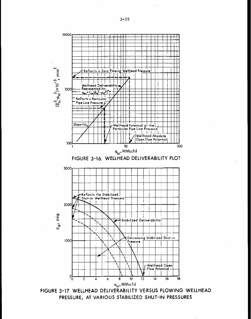
in some instances, the wellhead pressures may be plotted versus flow
rate in a manner similar to the sandface curses of Figures 3-1 or 3-2.
The relationship thus obtained Is known as the wellhead deliverability
and is shown in Figure 3-16. On logarithmic coordinates the slope of
the wellhead deLiverability plot is not necessarily equal to that
obtained using sandface pressures (Edgington and Cleland, 1967);
moreover, unless corrections are made, variations of the flowing
temperature in the wellbore may cause the plot to be a curve instead
of a straight line (Wentink et al. 1971).
A wellhrad deliverability plot is useful because it relates
to a surface situation, for example, the gathering pipeline back
pressure, which is mote accessible than the reservoir. However, it has
the disadvantage of not being unique for the well as it depends on the
size of the pipe, tubing or annulus, in which the gas is flowing.
MOEOVer, unlike the sandface relationship it does not apply throughout
the life of the well since the pressure drop in the wellbore itself is
a Eunctim not only of fl.ow rate but also of pressure level.
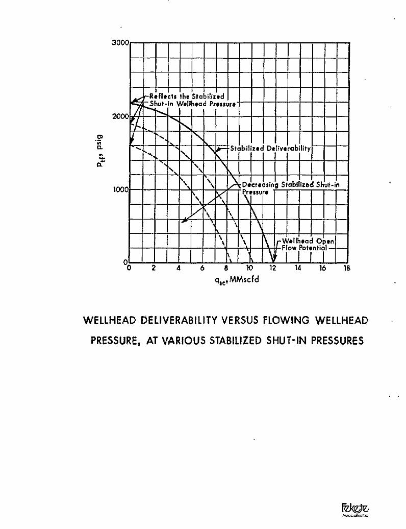
Because the wellhead deliverability relationship is not
constant throughout the life of a well, different curves are needed to
represent the different average reservoir pressures, as shown in Figure
3-17. At any condition of depletion represented by p,, the sandface
deliverability is valid and may be used to obtain the wrllhead
3-34
deliverability by converting the sandface pfess~res to wellhead
conditions using the method of Appendix B, in reverse.
7 IMPORTANT CONSIDERATIONS PERTAINING TO DELIVERABILITY TESTS
In all of the tests described so far, the time to stabilization
is an important factor, and is discussed in detail below. Moreover, the
flow rate is assumed to be constant throughout each flow period. This
condition is not always easy to achieve,in ptac'cice. The effect on
test results of a non-constant flow rate is considered In this section.
The choice of a sequence of increaslng or decreasing flow rates is also
discussed.
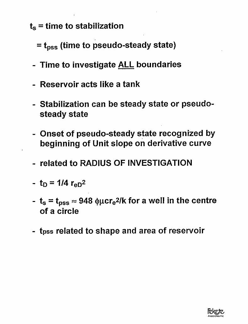
7.1 Time to Stabilization and Related Matters
Stabilization originated as a practical consideration and
reflected the time when the pressure no longer changed significantly
with time; that is, it had stabilized. With high permeability reservoirs
this point was not too hard to observe. However, with tight formations,
the pressure does not stabilize for a very long time, months and
sometimes years. MOreOVer, except where there is a pressure maintenance
mechanism acting on the pool, true steady-state is never achieved and
the pressure never becomes constant.
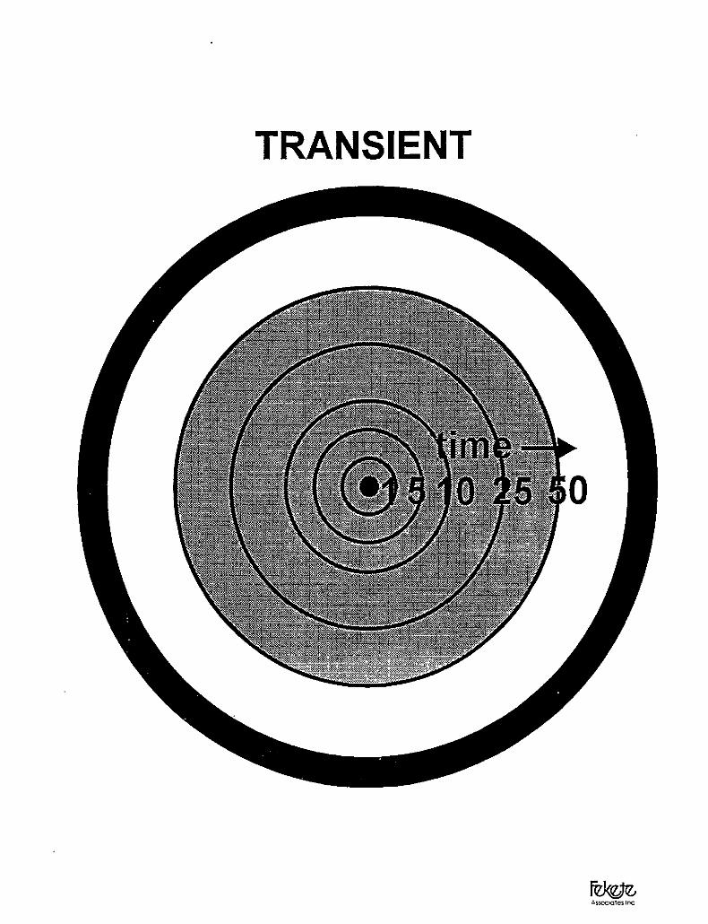
Stabilization is more properly defined in terms of a radius of
investigation. This is treated, in detail in Chapter 2, but will be
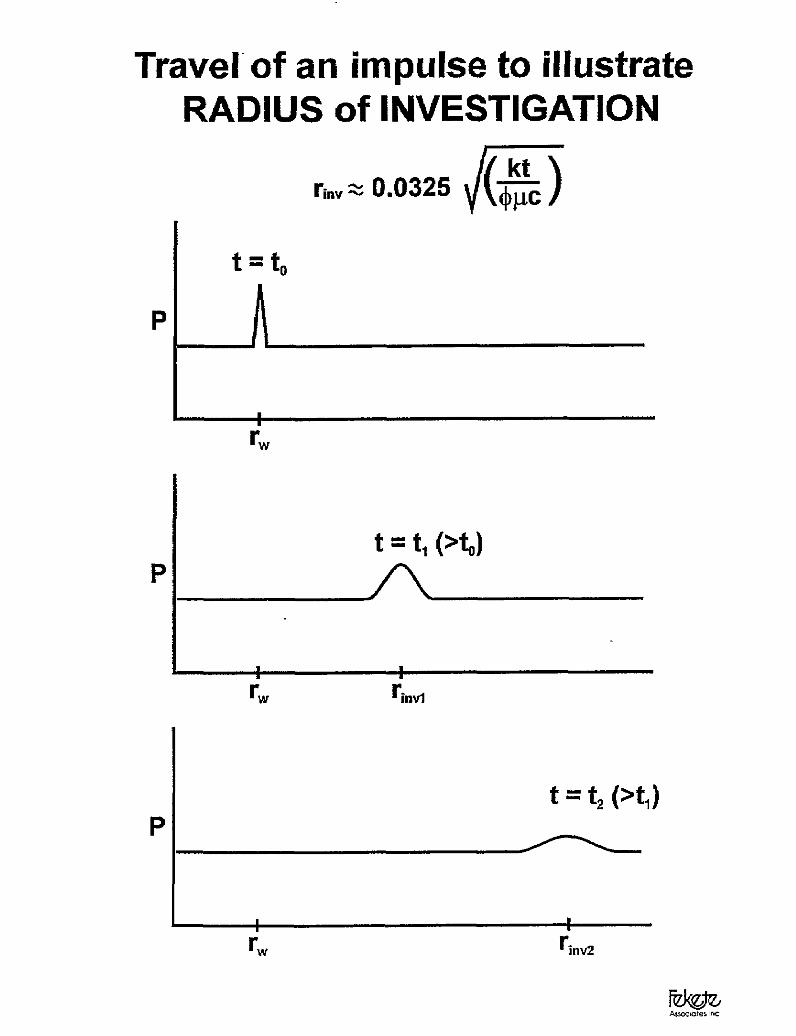
reviewed here. When a disturbance is initiated at the well, it will
have an immediate effect, however minimal, at all points in the
reservoir. At a certain distance from the well, however, the effect of
the disturbance will be so small as to be unmeasurable. This distance,
at which the effect is barely detectable is called the radius of
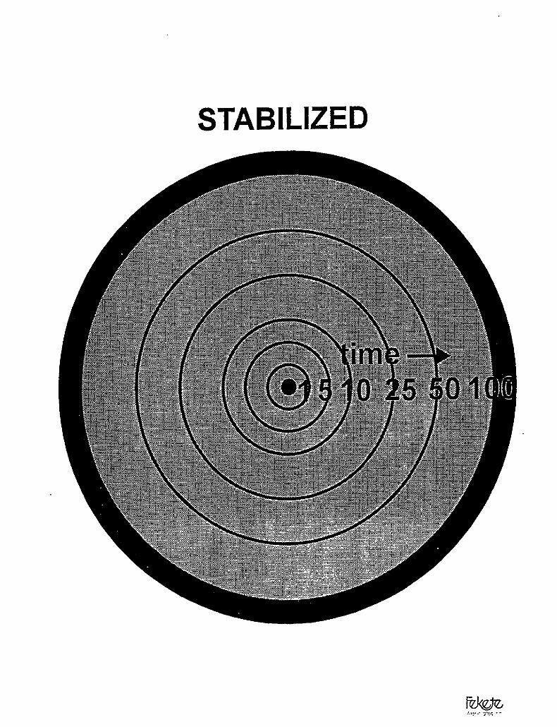
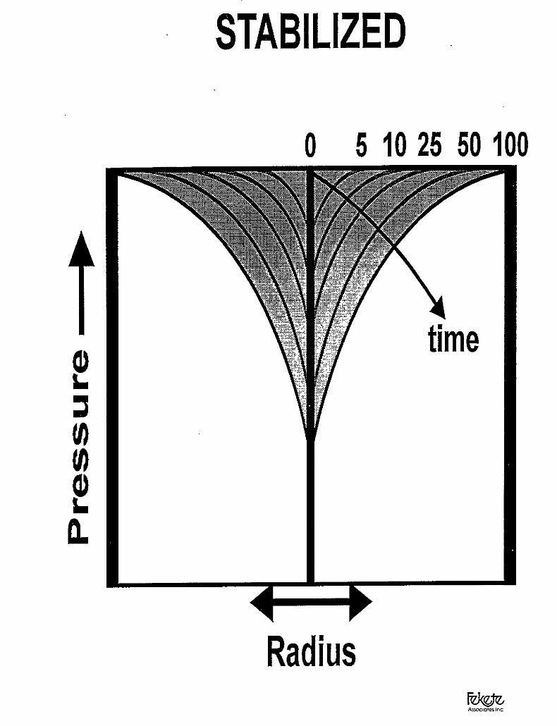
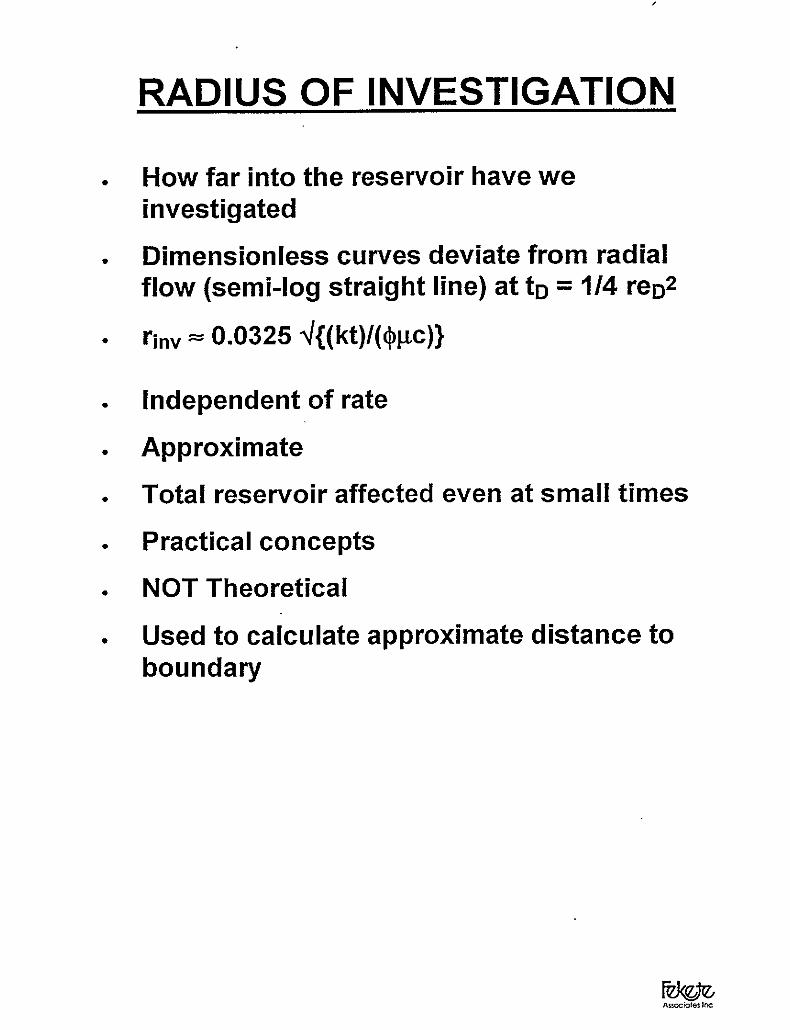
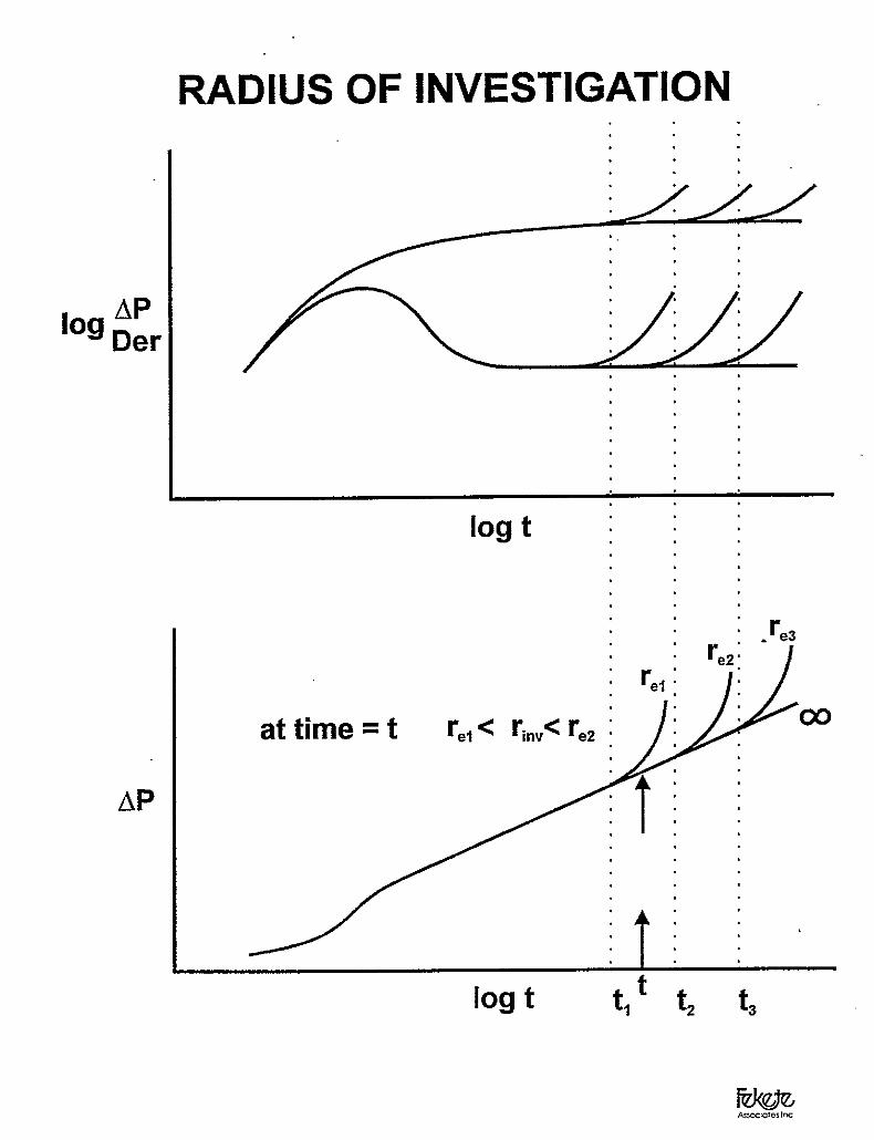
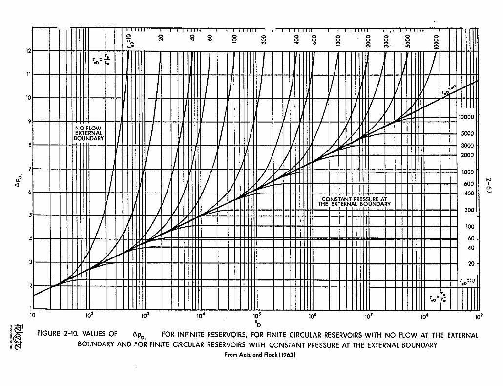
investigation, rinv. As time increases, this radius moves outwards into the formation until it reaches the outer boundary of the reservoir OF
the no-flow boundary between adjacent flowing wells. From then on, It
3-35
100 1 10 100
q,,, MMscfd
FIGURE 3-16. WELLHEAD DELIVERABILITY PLOT
3000
0 0 2 4 b 8 IO 12 14 lb 18
~7 MMscfd
FIGURE 3-1Z WELLHEAD DELIVERABILITY VERSUS FLOWING WELLHEAD PRESSURE, AT VARIOUS STABILIZED SHUT-IN PRESSURES
3-36
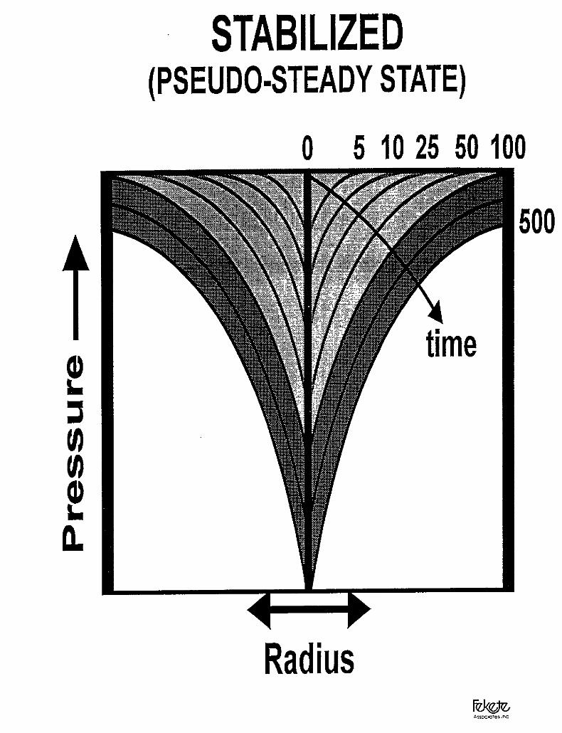
stays constant, that is, r inv = re* and stabilization Is said co have
been attained. This condition is also called pseudo-steady state.
The pressure does not become constant but the rate of pressure decline
does.
The time to stabilization can only be determined approximately
and is given by Equation (3N-15) as
(3-14)
where
ts, = time to stabilization, hr
r = e outer radius of the drainage area, ft
i; = gas viscosity at p,, cp
$ = gas-fllled porosity, fraction
k = effective permeability to gas, md
There exist various rule-of-thumb methods for determining when
stabilization is reached. These are usually based on a rate of pressure
decline. When the specified rate, for example, a 0.1 psi drop in 15
minutes, is reached, the well is sard to be stabilized. Such over-
simplified criteria can be misleading. It is shown in the Notes to this
chapter that at stabilization, the race of pressure decline at the well
is given by Equation (3N-19) as
(3-15)
This shows that the pressure decline in a given time varies
from well to well, and even for a particular well, it varies with the
flow rate. For these reasons, methods of defining stabilization which
make use of a specified rate of pressure decline may not always be
reliable.
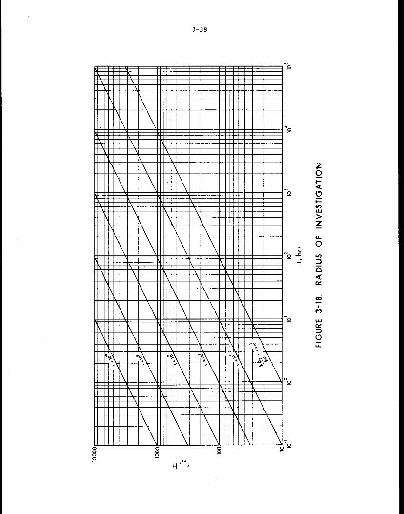
The radius of investigation, rinvf after t hours of flow is
given by Equation (3N-21). This equation is portrayed graphically in
Figure 3-18.
3-37
for rinv < re (3-M)
As long as the radius of investigation is less than the
exterior radius of the reservoir, stabilization has not been reached
and the flow is said to be transient. Since gas well tests often
involve interpretation of data obtained in the transient flow regime,
a review of transient flow seems appropriate. For transient flow,
Equations (3-l) and (3-4) still apply but neither C nor a IS constant.
Both C and a will change with time until stabilization is reached.
From this time on, C and a will stay constant.
Effective Drainage Radius
A concept which relates transient and stabilized flow
equations is that of effective drainage radius, rd, which is discussed
in detail in Chapter 2. It is defined 8s that radius which a
hypothetical steady-state circular reservoir would have if the pressure
at that radius were s R and the drawdown at the well at the given flow
rate were equal to the actual drawdown. Initially, the pressure drop
at the well increases and so does rd. Ultimately, when the radius of
investigation reaches the exterior boundary, re, of a closed reservoir,
the effective drainage radius is given by Equation (Z-101)
rd = 0.472 r e (3-17)
The above equation is the source of the popular idea that the
radius of drainage only moves half-way into the reservoir. It should
be emphasized that at all times, drainage takes place from the entire
reservoir and that r d is only an equivalent radius which converts an
unsteady-state flow equation to a steady-state one. Furthermore, the
distinction between the concepts of effective drainage radius and radius
of investigation should be understood as,described in Chapter 2,
Section 6.4.
3-38
-
3-39
7.2 Sequence of Flow Rates
The usual practice in conducting deliverability tests is
to use, where possible, a sequence of increasing flow rates. In a
conventional test, if there ig a likelihood of hydrates, forming, a
decreasing sequence is advisable as it results in higher wellbore
‘temperatures and a decreased tendency to form hydrates. Where liquid
hold-up in the wellbore is a problem, a decreasing sequence may be
preferred.
If the conventional fesf ,or the isochronal test are properly
conducted, that is, stabilization of pressure is observed before a new
rate Is selected, the rate sequence is imaterial. Either an increasing
or a decreasing sequence will give the true deliverability relationship.
Ilowever, for the modified isochronal test, an increasing rate sequence
should be used, otherwise the test method loses accuracy, and may not
be acceptable.
The extended flow rate of the isochronal or modified
isochronal test may be run either at the beginning, if the well is
already on production, or at the end of the test. If it is conducted
at the beginning, the well must then be shut in to essentially stabilized
conditions, prior to the commencement of the isochronal flow periods.
Often, the last isochronal rate is simply extended to stabilization, with
a pressure reading being taken at the appropriate (isochronal) time of
flow, and later at stabilization. However, this need not necessarily
be so. In fact, any suitable flow rate may be chosen with or without
a shut-in intervening between it and the last isochronal rate, as long
as the flow is extended to pressure stabilization.
7.3 Constancy of Flow Rate
In incerpretlng the theory applicable ‘co the tests described
so far, the flow tare within each flow period is assumed to be constant.
In practice this situation is rarely achieved. If the flow is being
measured through a critical flow prover, the upstream pressure declines
3-40
continuously with time, and hence the flow rate decreases correspondingly.
If an orifice meter is being used to measure the gas flow, the usual
prac’cice~is to set the choke, upstream of the orifice meter, at a fixed
setting. This setting is not changed throughout the flow period. A
declining wellhead pressure upstream of the choke coupled with a
constant pressure downstream of the choke, resulting from the back
pressure regulator, often results in a continuously declining flow
rate. Moreover, the calculations of flow rates involve the gas flowing
temperature. During short flow periods, the wellhead temperature is
rarely constant, the variation being due CO a gradual waraing up of the
well. All these factors make it difficult for an absolutely Constant
flow rate to be maintained.
Winestock and Colpitts (1965) developed a method of analysis
to account for the variations in flow rate. Lee, Harrell and McCain
(1972) confirmed, by numerical simulation, the validity of their
approach. The results of their study related to drawdown testing are
%amnarized in a later chapter, but some of the findings applicable to
deliverability tests are given below.
Provided the changes in flow rate are not excessively rapid,
instantaneous values of the flow rate and the corresponding flowing
pressure should be used rather than values averaged over the entire
flow period. In view of this, flow rates need not be kept absolutely
constant, but may be allowed to vary smoothly and continuously with
time, as is the case with flow provers or orifice meters. Since sudden
changes in rate invalidate this approach, IXI change in orifice plates
is permissible for whatever reason, not even in order to adhere to a
prespecified schedule, once a flow period has commenced.
8 GUIDELINES FOR DESIGNING DELIVERABILITY TESTS
Once the decision has been made to run a deliverability test,
all the information pertaining to the well and to the reservoir under
investigation should be collected and utilized in specifying the test
procedure. such information may include logs, drill-stem teats,
3-41
previous delrverabiliey testa conducted on that well, production
history, fluid composition and temperature, cores and geological
studies. In the absence of some of these derails, data from neighbouring
wells completed is the same formation may be substituted. At all times,
the value of first-hand field experience must not be underestimated and
should certainly have a major influence on the design and conduct of
tests.
8.1 Choice of Test
A knowledge of the time required for stabilization is a very
lmporrant factor in deciding the type of test Co be used for determining
the deliverabiliey of a well. This may be known directly from previous
tests, such as drill-stem or deliverability tests, conducted on the well
or from the production characteristics of the well. If such information
is not available, it may be assumed that the well will behave in a
manner similar to neighbouring wells in the same pool, for which the
data are available.
When the approximate time to stabilization is not known, It
may be estimated from Equation (3-14). If the time ‘co stabilization is
of the order of a few hours, a conventional test may be conducted.
Otherwise one of the isochronal ‘ce*Es is preferable. The isochronal
test is more accurate than the modified isochronal test and should be
used if the greater accuracy is warranted.
The choice of a test is discussed more fully in Chapter 1,
An important consideration is that if gas is to be flared, the duration
of the test should be minimized. This may be accomplishad by testing
only new exploratory wells, using isochtonal type teats rather than the
conventional deliverability test, and calculating the stabilized flow
point rather than flowing a well to stabilization. Where the well
being tested is tied into a pipellne, more flexibility is available in
choosing the type of test, but care must ‘be taken to ensure sufficiently
long flowperiodswhen stabilized flow points are to be obtained.
A single-point test is appropriate when the deliverability
3-42
relationship of the well is known from previous tests, and only updating
of this relationship is desired. A convenient time to conduct such a
test is prior to a shut-in for a pressure survey of the pool as the well
is probably stabilized and all that is needed is a measurement of the
flow rate and the flowing pressure.
8.2 Choice of Equipment
The various types of equipment used in gas well testing are
mentioned in Chapter 6. Some of the factors affecting the choice of
equipment are the expected flow rates and pressures, and the analysis
of the gas and liquid effluent to be expected during the test. The
possibility and location of hydrate formation must be investigated.
This may be done by the methods outlined in Appendix A and wiJ.1 affect
the choice of the heating equipment to be used during the test. Failure
to prevent hydrate formation will result in enomaLous flow data due to
complete or partial plugging of sections of the equipment.
Production of liquid, be it water or condensate, causes
fluctuations in the rate and pressure measurements. Long flow times,
of at least six to eight hours, are needed before the liquid to gas
ratio stabilizes. One or two separators at the surface must be included
in the test equipment since the gas must be free of liquid before it can
be measured with the standard orifice meters or critical flow provers.
Calculations of sandface pressures from wellhead pressures become
inaccurate when there is liquid in the wellbore and wherever practically
possible the use of bottom hole pressure bombs becomes mandatory.
Extremely sour gases may make the use of bottom hole equipment
impossible because of problems with corrosion or sulphur deposition.
8.3 Choice of Flow Rates
1n conducting a multi-point test, the minimum flow rate used
should be at least equal to that required to lift the liquids, if any,
from the well. It should also be sufficient to maintain a wellhead
temperature above the hydrate point, Where these considerations do not
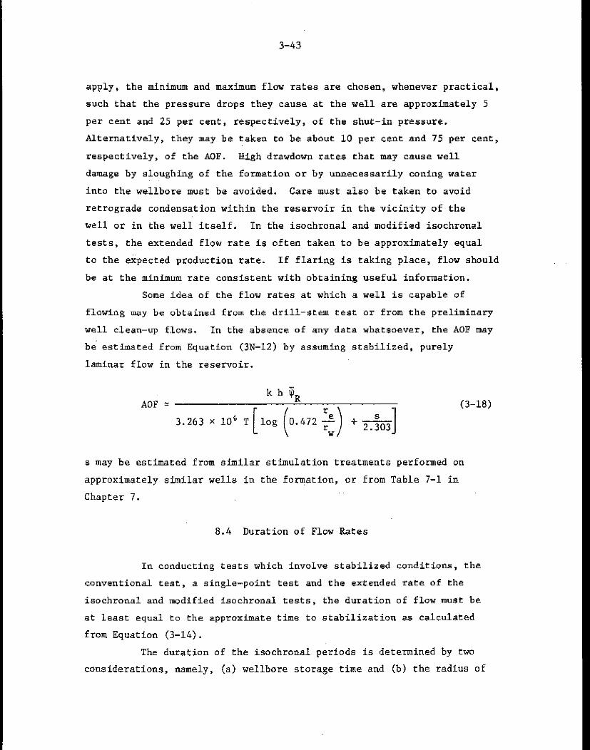
3-43
apply, the minimum and maximum flow rates are chosen, whenever practical,
such that the pressure drops they cause at the well are approximately 5
par cent and 25 per cent, respectively, of the shut-in pressure.
Alternatively, they may be taken to be about 10 per cent and 75 per cent,
respectively, of the AOF. High drawdown rates that may cause well
damage by sloughing of'the formation or by unnecessarily coning water
into the wellbore must be avoided. Care must also be taken to avoid
retrograde condensation within the reservoir in the vicinity of the
well or in the well itself. In the isochronal and modified isochronal
tests, the extended flow rate is often taken to be approximately equal
to the expected production rate. If flaring is taking place, flow should
be at the mlnLmum rate consistent with obtaining useful information.
Some idea of the flow rates at which a we13 is capable of
flowing may be obtained from the drill-stem test or from the preliminary
well clean-up flows. In the absence of any data whatsoever, the AOF may
be estimated from Equation (3N-12) by assuming stabilized, purely
lamisar flow in the reservoir.
AOF = k h qR
3.263 x lo6 T[l,, (0.472 $) + &]
(3-18)
s may be estimated from similar stimulation treatments performed on
approximately similar wells in the formation, or from Table 7-l in
Chapter 7.
8.4 Duration of FLOW Rates
In conducting tests which involve stabilized conditions, the
conventional test, a single-point test and the extended rate of the
isochronal and modified isochrcnal tests, the duration of flow must be
at least equal to the approximate time to stabilization as calculated
from Equation (3-14).
The duration of the isochronal periods is determined by two
considerations, namely, (a) wellbore storage time and (b) the radius of
3-44
investigation.
a. The wellbore storage time, tws, it the approximate time
required for the wellbore storage effects to become negligible. This
can be calxulated from Equation (3N-24) which is developed in the Notes
to this chapter:
t 36177 ii vws cws
= "* kh O-19)
where
v = ws volume of the wellbare tubing (and aanulus, if there
is no packer)
c = ws compressibility of the wellbore fluid evaluated at
the mean wellbore pressure and temperature
Equation (3-19) is presented graphically in Figure 3-19 for the case
of a three-inch internal diameter tubing string in a six-inch internal
diameter casing, with and without an annulus packer.
b. The radius of investigation has been discussed in Section
7.1. Rarely does wellbore damage or stimulation extend beyond 100 feet.
In order to obtain data that are representacive.of the formation, the
flow period must last longer than the time to investigate the first 100
feet. For wells wlrh no damage or improvement an approximate time to
investigate 100 feet is obtained from Equation (3-X) or from Figure
3-18. From Equation (3-14)
t loo = 1000 $ loo2 = 1.0 x lo7 $ R R
(3-20)
The greater of tws and tlOO is the minimum duration of flow that will
yield data representative of the bulk formation rather than the wellbore
area. A duration equal to about four times this value is recommended
for the isochronal periods.
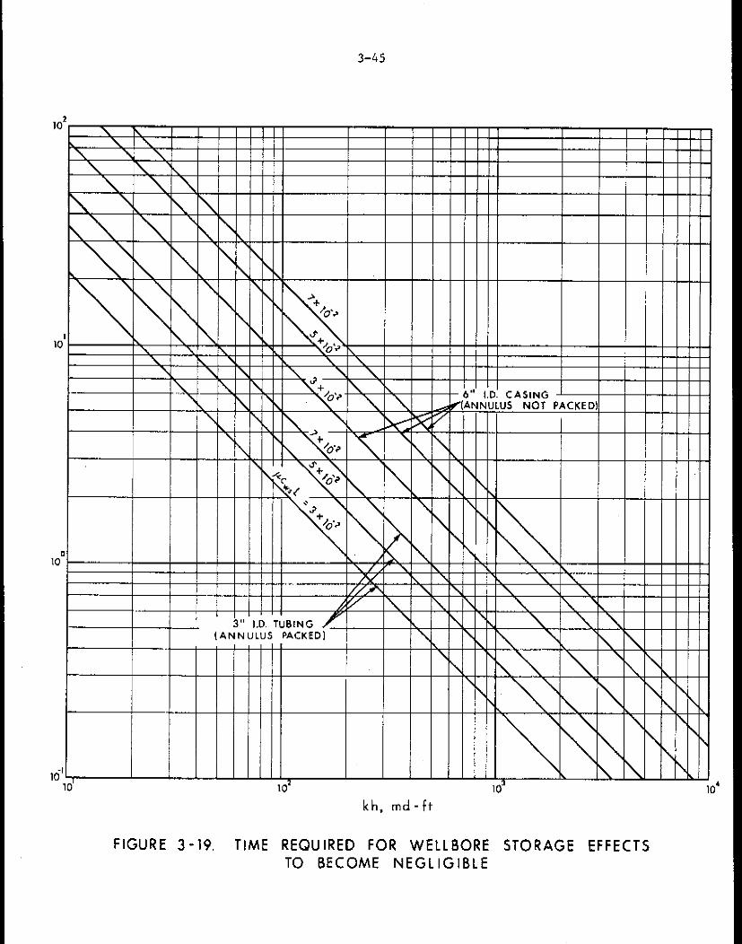
3-45
- - -
-
-
- -
-
Z Y -
\
7
\ - -
t - -
\ -
-
-
kh, md-ft
tus NOT PACKED
- - - - - - - - -
- - - - - - - - -
- - - - s \ - \ - \ *
FIGURE 3-19. TIME REQUIRED FOR WELLBORE STORAGE EFFECTS TO BECOME NEGLIGIBLE

3-46
EXAMPLE 3-6
Introduction This example illustrates calculations that are essential
to the design of a deliverability test.
Problem A well was completed in a dry, sweet gas pool which is being
developed with a one-section spacing between wells. It has been cored,
logged and drill-stem tested, acidized and cleaned but no deliverability
tests have, so far, been performed on it. Design a suitable
deliverability test.
Solution
Choice of Test
Before the choice of a suitable test can be made, the
approximate time to stabilization, t S' must be known. This being the
first well in the pool, and the drill-stem test flow rate not being
stabilized, the time to stabilization is not known and should be
estimated from Equation (3-,14). This requires a knowledge of the
Following factors: re' P,, $9 k, i,
= 2640 ft, equivalent to a one-section spacing;
= 2000 psia, obtained from the drill-stem test;
= 0.15, the gas filled porosity is obtained by
multiplying the formation porosity by the gas
saturation, both quantities being deducible
from logs:
= 120 md, the build-up period of the drill-stem
test was analyzed by methods described in Chapter 5
to give an effective kh = 1200 md-ft. From logs,
h = 10 ft;
= 0.0158 cp, the gas composition is known and is the
same as that of Example A-l. The reservoir
temperature is 580%.
From Equation (3-14)
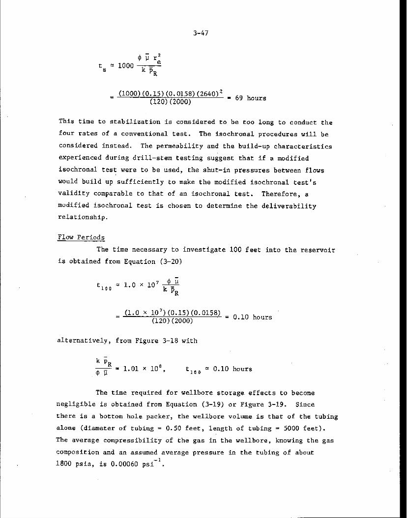
3-47
= (looo)(o.15)(o.o158)(2640~2 _ 69 hours (120) (2000)
This time to stabilization is considered to be too long to conduct the
four rates of a conventional test. The isoehronal procedures will be
considered instead. The permeability and the build-up characteristics
experienced during drill-stem testing suggest that if P modified
isochronal test were to be used, the shut-in pressures between flows
would build up sufficiently to make the modified isochronal test's
validity comparable to char of an isochronal test. Therefore, a
modified isochronal test is chosen to determine the deliverability
relationship.
Flow Periods
The time necessary to investigate 100 feet into the reservoir
is obtained from Equation (3-20)
t 100 = 1.0 x lo7 *
R
se (1.0 x 10’)(0.15)(0.0158) = o 1o hours (120) (2000)
alternatively, from Figure 3-18 with
k PR
@D 1.01 x lOa, t lpo = 0.10 hours
The time required for wellbore storage effects to become
negligible is obtained from Equation (3-19) or Flgure 3-19. SiIlC@
there is a bottom hole packer, the wellbore volume is that of the tubing
alone (diameter of tubing = 0.50 feet, length of tubing = 5000 feet).
The average compressibility of the gas in the wellbore, knowing the gas
composition and an assumed average pressure in the tubing of about
1800 psia, is 0.00060 psi-l.
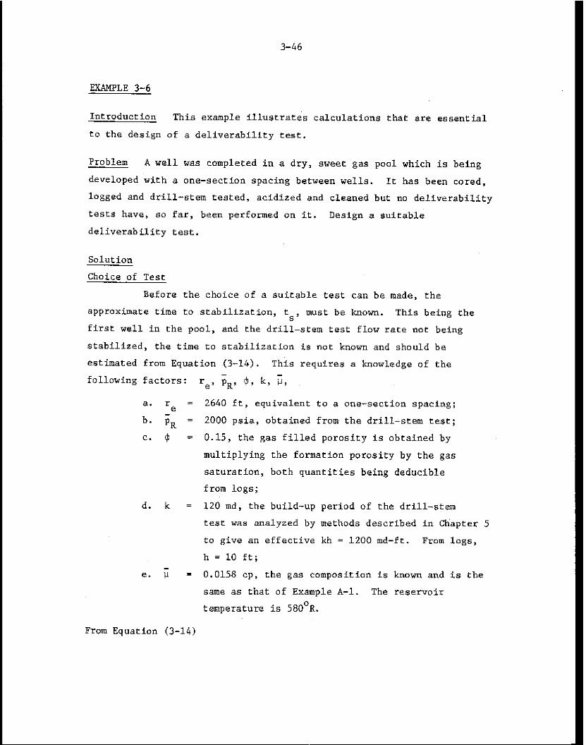
3-46
EXAMPLE 3-6
Introduction This example illustrates calculations that are essential
to the design of a deliverability test.
Problem A well was completed in a dry, sweet gas pool which is being
developed with a one-section spacing between wells. It has been cored,
logged and drill-stem tested, acldized and cleaned but no deliverability
tests have, so far, been performed on it. Design a suitable
deliverability test.
Solution
Choice of Test
Before the choice of a suitable test can be made, the
approximate time to stabilization, t 6' must be known. This being the
first well in the pool, and the drill-stem test flow rate not being
stabilized, the time to stabilization is not known and should be
estimated from Equation ,(3-14). This requrres a knowledge of the
following factors: re' $9 $7 k, L,
2640 ft, equivalent to a one-section spacing;
2000 psia, obtained from the drill-stem test;
0.15, the gas filled porosity is obtained by
multiplying the formation porosity by the gas
saturation, both quantities being deducible
from logs;
120 md, the build- up period of the drill-stem
test was analyzed by methods described in Chapter 5
to give an effective kh = 1200 md-ft. From logs,
h = 10 ft;
0.0158 cp, the gas composition is known. and is the
same as that of Example A-l. The reservoir
temperature is 580'R.
a. c =
b. ;; =
C. 9 =
d. k =
e. ; -
From Equation (3-14)
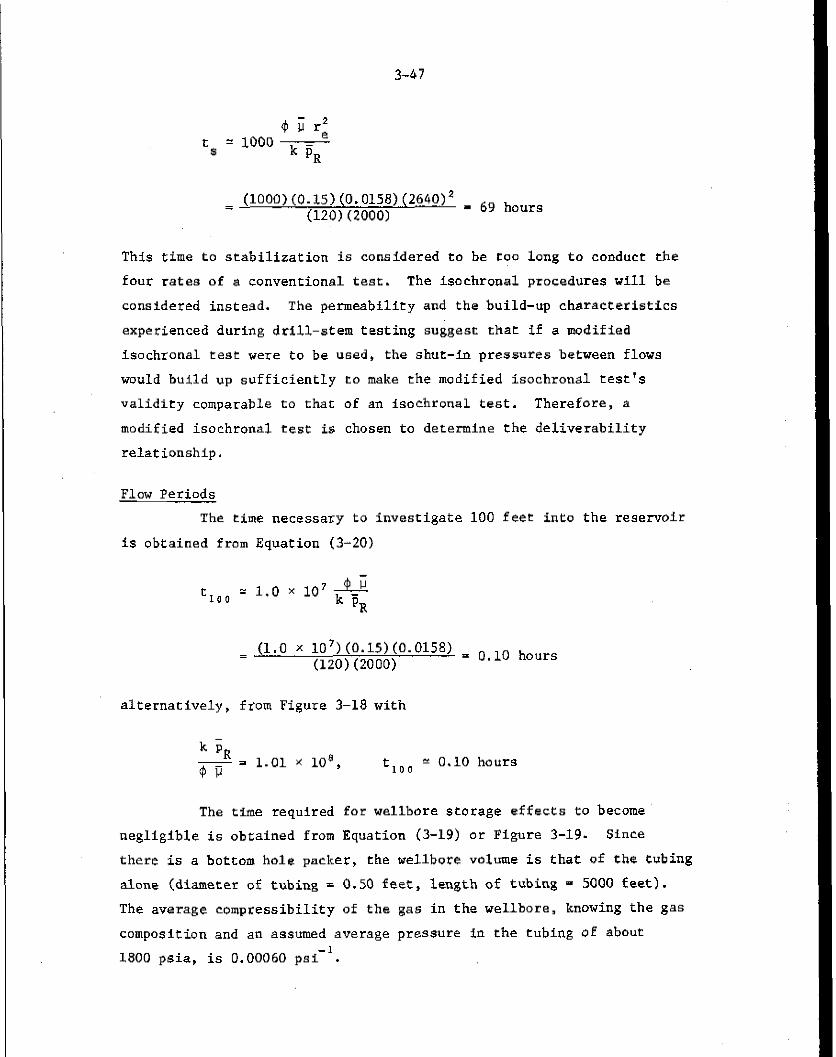
3-47
= (1000)(0.~5)(0.015E)(2640)2 _ 6g hours (120)(2000)
This time to stabilization is considered to be too long to conduct the
four rates of a conventional test. The isochronal procedures will be
considered instead. The permeability and the build-up characteristics
experienced during drill-stem testing suggest that If a modified
isochronal test were to be used, the shut-in pressures between flows
would build up sufficiently to make the modified isochronal test's
validity comparable to that of an isochronal test. Therefore, a
modified isochronal test is chosen to determine the deliverability
relationship.
Flow Periods
The time necessasy to investigate 100 feet into the reservoir
is obtained from Equation (3-20)
c 100 = 1.0 x 10's R
= (1.0 x 10')(0.15)(0.015s) = o 1o ho"rs (120)(2000)
alternatively, ftom Figure 3-18 with
k iR m= 1.01 x loa, t loo = 0.10 hours
The time required for wellbore storage effects to become
negligible is obtained from Equation (3-19) or Figure 3-19. since
there is a bottom hole packer, the wellbore volume is that of the tubing
alone (diameter of tubing = 0.50 feet, length of tubing = 5000 feet).
The average compressibility of the gas in the wellbore, knowing the gas
composition and an assumed average pressure in the tubing of about
1800 psia, is 0.00060 psi-l.
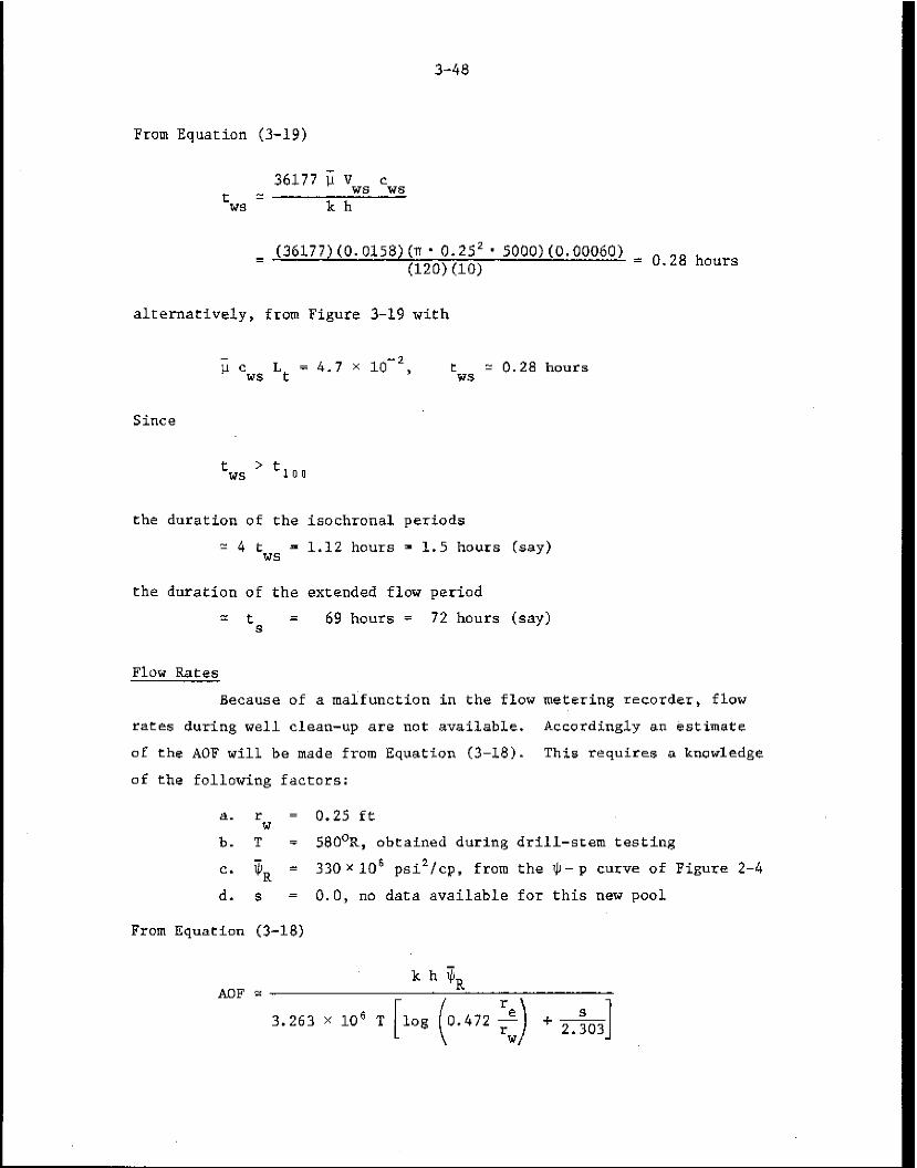
3-48
From Equation (3-19)
t 36177 u U", cws
ws kh
= (36177)(0.015a)(n* 0.25" 5000)(0.00060) = o.28 hours (120) (10)
alternatively, from Figure 3-19 with
; cw* Lt = 4.7 x 1o-2, t = 0.28 hours "S
Since
the duration of the isochronal. periods
=4t = 1.12 hours = ws 1.5 hours (say)
the duration of the extended flow period zt =
s 69 hours = 72 hours (say)
Flow Rates
Because of a mal.function in the flow metering recorder, flow
rates during well clean-up are not available. Accordingly an estimate
of the AOF will be made from Equation (3-W. This requires a knowledge
uf the following factors:
il. r = 0.25 fr
b. TW = 580°R, obtained during drill-stem testing
C. TR = 330x10" psi'/cp, from the Q-p curve of Figure 2-4
d. s = 0.0, no data available for this new pool
From Equation (3-18)
AOF z: k h Ji,
3.263 x lo6 T [log (0.47, ;) + &]
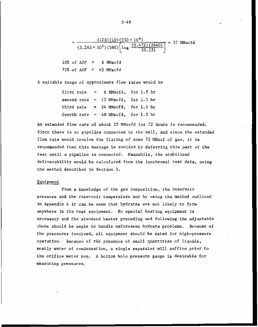
3-49
=e (120)(10)(330 r105)
(3.263x10⁶)(580) log ‘“.4:;‘;:;40’] = 57 MMscfd
10% of AOF = 6 MMscfd
75% of AOP = 45 Mi%cfd
A suitable range of approximate flow rates would be
first rate = 6 MMscfd, for 1.5 hr
second rate = 12 MNscfd, for 1.5 hr
third rate - 24 MMscfd, for 1.5 hr
fourth rate = 48 MMscfd, for 1.5 hr
An extended flow rate of about 25 MMscfd for 72 hour8 is recommended.
Since there is no pipeline connected to the well, and since the extended
flow rate would involve the flaring of some 75 MMscf of gas, it is
recommended that this wastage be avoided by deferring this part of the
test until a pipeline is connected. Meanwhile, the stabilized
deliverability would be calculated from the isochronal test data, using
the method described is Section 5.
Equipment
From a knowledge of the gas composition, the reservoir
pressure and the reservoir temperature and by using the method outlined
in Appendix A it can be seen that hydrates are not Likely CO form
anywhere in the test equipment. No special heating equipment is
necessary and the standard heater preceding and following the adjustable
choke should be ample to handle unforeseen hydrate problems. Because of
the pressures involved, all equipment should be rated for high-pressure
0peratioIl. Because oE the presence of small quantities of liquids,
mostly water of condensation,.a single separator will suffice prior to
the orifice meter run. A bottom hole pressure gauge is desirable for
measuring pressures.
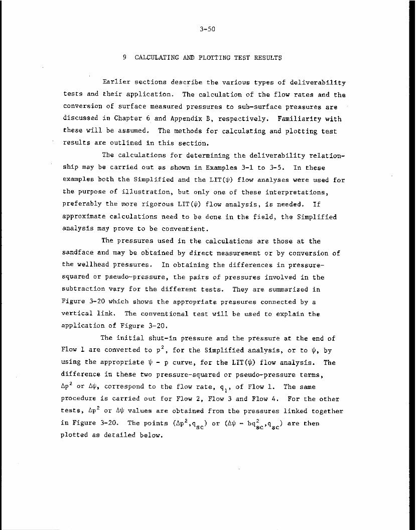
9 CALCULATING ANTJ PLOTTING TEST RESULTS
Earlier sectione describe the various types of deliverability
tests and their application. The calculation of the flow rates and the
conversion of surface measured pressures CD sub-surface pressures are
discussed in Chapter 6 and Appendix B, respectively. Familiarity with
these will be assumed. The methods for calculating and plotting test
results are outlined fn this sectidn.
The calculations for determining the deliverability relation-
ship mey be carried out as shown in Examples 3-1 to 3-5. In these
examples both the Simplified and the LIT($) flow analyses were used for
the purpose of illustration, but only one of these interpretations,
preferably the more rigorous LIT($) flow analysis, is needed. If
approxWate calculations need to be done in the field, the Simplified
analyeis inay prove to be conventient.
The pressures used is the calculations are those at the
sandface and may be obtained by direct measurement or by conversion of
the wellhead pressures. In obtaining the differences in pressure-
squared or pseudo-pressure, the pairs of pressures involved in the
subtraction vary for the different tests. They are summarized in
Figure 3-20 which shows the appropriate pressures connected by a
vertical link. The conventional test will be used to explain the
application of Figure 3-20.
The initial shut-ln pressure and the pressure at the end of
Flow 1 are converted to p', for the Stmplified analysis, or to $, by
using the appropriate $ - p curve, for the LIT($) flow analysie. The
difference in these two pressure-squared or pseudo-pressure terms,
AP' Of 4, correspond to the flow rate, q,, of Flow 1. The came
procedure is carried out for Flow 2, Flow 3 and Flow 4. For the other
tests, Ap' or A$ values are obtained from the pressures linked together
in Figure 3-20. The points (Ap2,q,,) or (AIJJ - bq&,q,,) are then
plotted as detalled below.
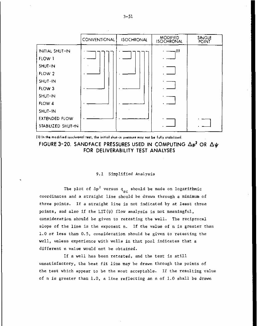
3-51
INITIAL SHUT-IN
FLOW 1
SHUT-IN
FLOW 2
SHUT-IN
FLOW 3
SHUT-IN
FLOW 4
SHUT-IN
EXTENDED FLOW
STABILIZED SHUT-IN
:ONVENTlONAL ISOCHRONAL MODIFIED ISOCHRONAL
I I
’ : 7”’ .--J :I :I
‘I I I
(I) In tha modified irochronol test, the initial shut-in preraure may not bs fully stabilized.
:Il
FIGURE 3-20. SANDFACE PRESSURES USED IN COMPUTING Ap2 OR A$ FOR DELIVERABILITY TEST ANALYSES
9.1 Simplified Analysis
The plot of Ap' versus q,, should be made on logarithmic
coordinates and a straighr line should be drawn Khrough a minimum of
three points. If a straight line is not Indicated by at least three
points, and also if the LIT($) flow analysis is not meaningful,
consideration should be given to retesting the well. The reciprocal.
slope of the line is the exponent n. If the value of n is greater Khan
1.0 or less than 0.5, consideration should be given to retesting the
well, unless experience with wells in that pool indicates Khat a
different n value would not be obtained.
If a well has been retesred, and the test ls still
unsatisfactory, the best fit line may be drawn through the points of
the test which appear to be the most acceptable. If the resulting value
of n is greater than 1.0, a line reflecting an n of 1.0 shall be dram
3-52
through the highest flow rate point. If the value of n Is less than
0.5, a line reflecting an n of 0.5 shall be drawn through the lowest
flow rate point.
In the case of isochronal type tests the deliverability line
should be positioned to reflect stabilized conditions. This 1~ done by
plotting the stabilized value of Ap’ versus the appropriate flow rate.
A line,of reciprocal slope n Is drawn through the point, a8 is
illustrated in Figure 3-8.
9.2 LIT($) FLOW Analysis
The deliverability relationship represented by Equation (3-4)
should be determined by calculating a and b from Equations (3-7) and
(3-E). A plot of (AIJJ - bqic) versus p,, on logarithmic coordinates
should be made with the data points and the calculated deliverability
relationship. Any data points showing ari excessive deviation from the
straight line plotted should be rejected, and the entire procedure of
calculating a, at or b should be repeated with at least three data
points. If the scatter of data points is excessive or if b is negative,
consideration should be given to retesting the well, unless experience
with wells in that pool indicates that a different line would not be
obtained.
If the well has been retested, and the test is still
unsatisfactory, a least squares fit of the data points that appear most
acceptable should be made. If at or b still turn out to be negative,
then a value of zero should be used in place of the negative number.
These two condi,tions are equivalent to n = 1.0 (for b = 0) and n = 0.5
(for a = 0) in the Simplified analysis.
In any case, the relationship resulting from this second
unsatisfactory test is only an estimated one, and consideration should
be given to a retest wrthin a one-year period. The fetest should
involve alterations in test procedure in an attempt to obtarn a
satisfactory relationship. This change may involve direct sandface
pressure measurements if two-phase flow appears to be a possibility, or
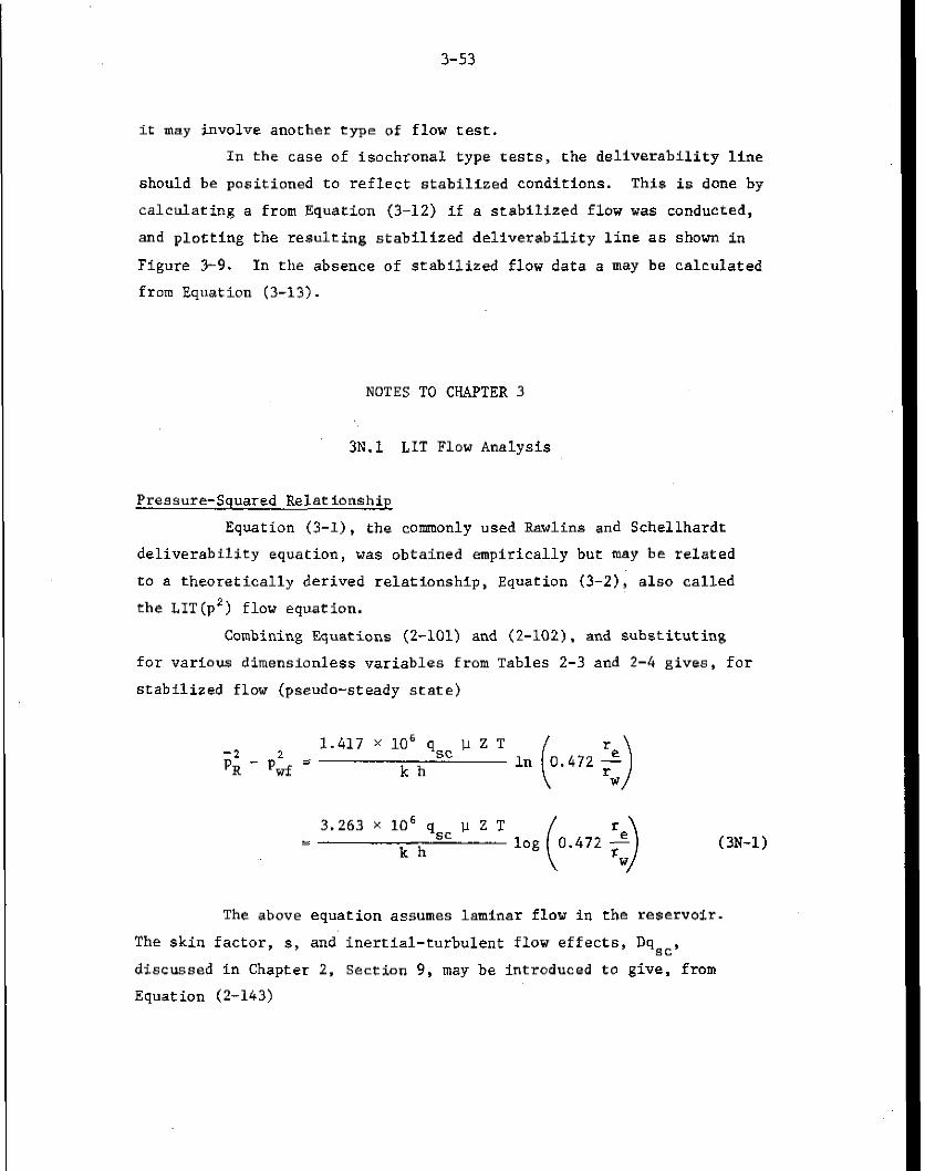
3-53
it may involve another type of flow test.
In the case of isochronal type rests, the deliverability line
should be positioned to reflect stabilized conditions. This is done by
calculating a from Equation (3-12) if a stabilized flow was conducted,
and plotting the resulting stabilized deliverability line a6 shown in
Figure 3-9. In the absence of stabilized flow data a may be calculated
from Eqvation (3-13).
NOTES TO CHAPTER 3
3N.1 LIT Flow Analysis
Pressure-Squared Relationship
Equation (3-l), the commonly used Rawlins and Schellhardt
deliverability equation, was obtained empirically but may be related
to a kheoretically derived relationship, Equation (3-2), also called
the LIT(p2) flow equation.
Combining Equations (2-101) and (2-102). and substituting
for various dimensionless variables from Tables 2-3 and 2-4 gives, for
stabilized flow (pseudo-steady state)
1.417 x lo6 -2 2 q SC u z T PR - P,f = kh
3.263 x lo6 qsc p z T %
kh (3N-1)
The above equation assumes laminar flow in the reservoir.
The skis factor, s, and inertial-turbulent flow effects, DqsC,
discussed in Chapter 2, Section 9, may be introduced to give, from
Equation (2-143)
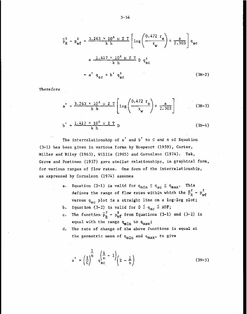
3-'54
-2 2 PR - P,f = 3.263XX1~'YZT[log(o.4::re)+~]q*c
+ 1.417 x 10⁶ II Z T kh D q:c
, a q,, + b' qic, (3N-2)
Therefore
(3N-3)
bl = 1.417 x IO6 v 2 T kh
D (3N-4)
The interrelationship of a' and b' to C and n of Equation
(3-l) has been given in various forms by Houpeurt (1959), Carter,
Miller and Riley (1963), Willis (1965) and Cornelson (1974). Tek,
Grove and Poetrman (1957) gave similar relationships, in graphical form,
for various ranges of flow rates. One form of the interrelationship,
as expressed by Cornelson (1974) assumes
a. Equation (3-l) is valid for qmin 2 qsc C q,,,. This
defines the range of flowrates within which the Fi - p$
Versus'q,, plot is a straight line on a Log-log Plot;
b. Equation (3-2) &valid for 0 2 q,, 5 AOP;
c. The function ;;; - p& from Equations (3-l) and (3-Z) is
equal with the range qmin to qmax;
d. The rate of change of the above functions is equal at
the geometric mean of qmin and q,,,, to give
(3N-5)
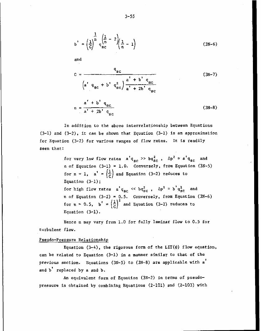
3-55
and
c= 4 *c
+ b’ qic a’ + b’ qsc
a’ + 2b’ q,,
ar + b’ qsc *=
a’ t 2b’ qs,
(3N-6)
ON-l)
(3N-8)
In addition to the above interrelationship between Equations
(3-l) and (3-2), it can be shown chat Equation (3-l) is an approximation
for Equation (3-2) for various ranges of flow rates. It IS readily
seen that:
for very low flow rates a’qsc .> bq;, , Ap’ = a’q,, and
n of Equation (3-l) = 1.0. Conversely, f ram Equation UN-5)
for n = 1, a’ = I3 and Equation (3-2) reduces to
Equation (3-l) :
for high flow rates a’qsc << bq& , Apz = b’q;, and
n of Equation (3-Z) = !.5* Conversely, from Equation (3~-6)
for n = 0.5, b’ = ($) and Equation (3-2) reduces to
Equation (3-l).
Hence n may vary from 1.0 for fully laminar flow to 0,5 for
turbulent flow.
Pseudo-Pressure Relationship
Equation (3-4). the rigorous form of the LIT($) flow equation,
can be related to Equation (3-l) in a manner similar to that of the
previous section. Equations (3N-5) to (3N-8) are applicable with a’
and b’ replaced by a and b.
An equivalent form of Equation (3N-2) in terms of pseudo-
pressure is obtaiaed by combining Equations (2-101) and (2-103) with
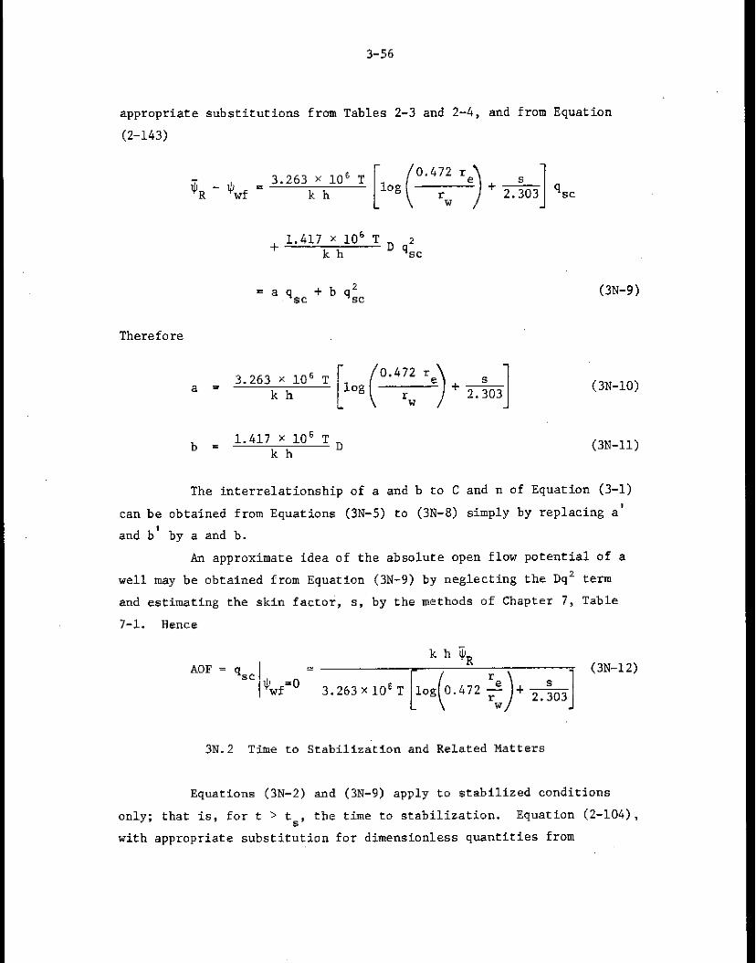
3-56
appropriate substitutions from Tables 2-3 and 2-4, and from Equation
(2-143)
f 1.417 x lo6 T kb D Gc
= a q*, + b qic (38-9)
Therefore
a - 3-263;;@ T [10g(o’4;; ‘@) + h] (3N-10)
b = 1.417 x lo6 T D
kh (3N-11)
The interrelationship of a and b to C and n of Equation (3-l)
can be obtained from Equations (3N-5) to (3N-8) simply by replacing a'
and b' by a and b.
An approximate idea of the absolute open flow potential of a
well may be obtarned from Equation (3N-9) by neglecting the Dq' term
and estimating the skin factor, s, by the methods of Chapter 7, Table
7-1. Hence
AOF = qsc k h 5,
E
%-" 3.263 x IO6 T [h+.472 ;)+ *] (3N-12)
3N.2 Time to Stabilization and Related Matters
Equations (3N-2) and (3N-9) apply to stabilized conditions
only; that is, for t > ts, the time to stabilization. Equation (2-104),
with appropriate substitution for dimensionless quantities from
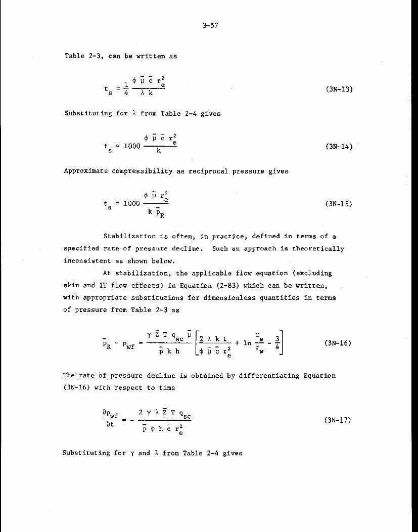
3-57
Table 2-3, can be written aa
,Substituting for x from Table 2-4 gives
Approximate compressibility ae reciprocal pressure gives
ON-131
(3N-14)
ts 2 1000 $ P r; k iR
(3N-15)
Stabilization is often, in practice, defined in terms of a
specified rate of pressure decline. Such an approach is theoretically
inconsistent as shown below.
At stabilization, the applicable flow equation (excluding
skin and IT flow effects) in Equation (2-83) which can be written,
with appropriate substitutions for dImensionless quantities in terms
of pressure from Table 2-3 as
PR - P”f =
The rate bf pressure
(3N-16) with respect
decline is obtained by differentiating Equation
to time
(3N-17)
Substituting for y and h from Table 2-4 gives
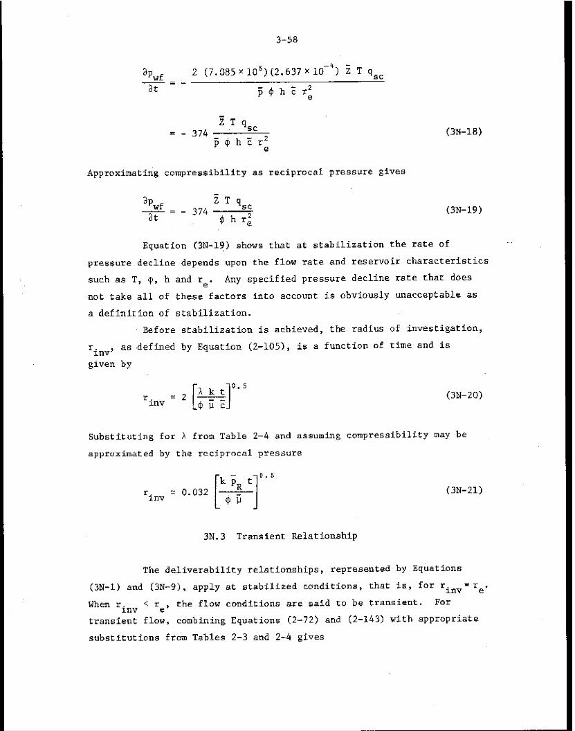
3-58
apwf 2 (7.385x10⁵)(2.637X10-') 2 T qsc -=-
at F$h?r;
Approximating compressibility as reciprocal pressure gives
(3N-18)
(3N-19)
Equati.on (3N-19) shows that at stabilization the rate of
pressure decline depends upon the flow rate and reservoir characteristics
such as T, $, h and re. Any specified pressure decline rate that does
not take all of these factors into account is obviously unacceptable as
a definition of stabilization.
Before stabilization is achieved, the radius of investigation,
r. XIV as .dcfined by Equation (2-105), is a function of time and is
given by
(3N-20)
Substituting for X from Table 2-4 and assuming compressibility may be
approximated by the rcciprocnl pressure
r. 1, n-9 = 0.032 (3N-21)
3N.3 Transient Relationshlp
The deliverability relationships, represented by Equations
(3N-1) and (3N-9), apply at stabilized conditions, that is, for rinv=re.
When rinv c re, the flow conditions are said to be transient. For
transient flow, combining Equations (2-72) and (2-143) with appropriate
substitutions from Tables 2-3 and 2-4 gives
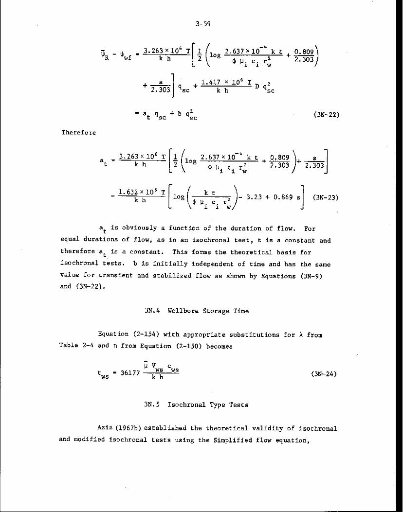
% - $"f - 3.263X10⁶ T
k h log 2.637X1O-4 k t + 0.809
+ !Ji ci r; 2.303
+k 'SC + I’ 1.417 x lo6 T k h D q:c
= at 4,. + b qic (3N-22)
Therefore
at is obviously a function of the duration of flow. For equal durations of flow, as in an isochronal test, t is a constant and
therefore at is a constant. This forms the theoretical basis for
isochronal tests. b is initially Independent of time and has the same
value for transient and stabilized flow as shown by Equations (3N-9)
and (3N-22).
3N.4 Wellbore Storage Time
Equation (2-154) with appropriate substitutions for h from
Table 2-4 and 0 from Equation (2-150) becomes
(38-24)
3N.5 Laochronal Type Tests
Aziz (1967b)established the theoretical validity of isochronal
and modified isochronal tests using the Simplified flow equation,
3-60
Equafion (3-l), radial unsteady-state laminar flow equations and several
simplifying assumptions. Noting that in the publication by Aziz (L967),
Modified Isochronal Testing and,Another Modification of the Isochronal
Test should be reversed since the latter is actually the proper modified
isochronal test, the theoretical justification may be extended quite
simply to include the LIT(e) flow equation, Equation (3-4), skin and IT
flow effects. Such an analysis would, however, assume that the
principle of superposition may be applied CO the unsteady-state LIT flow
equation.

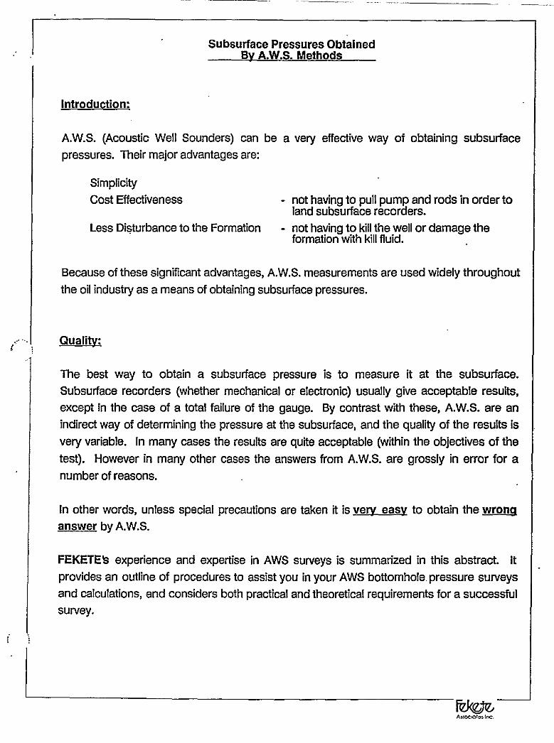
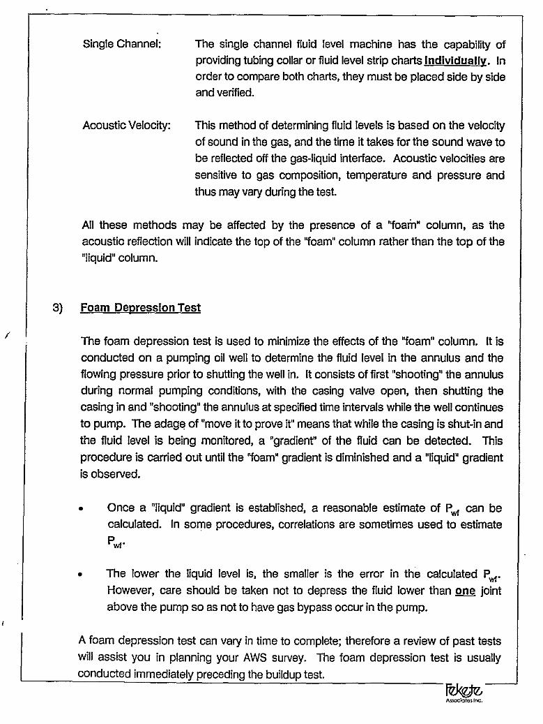
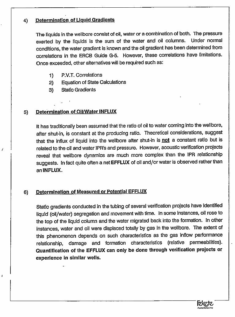
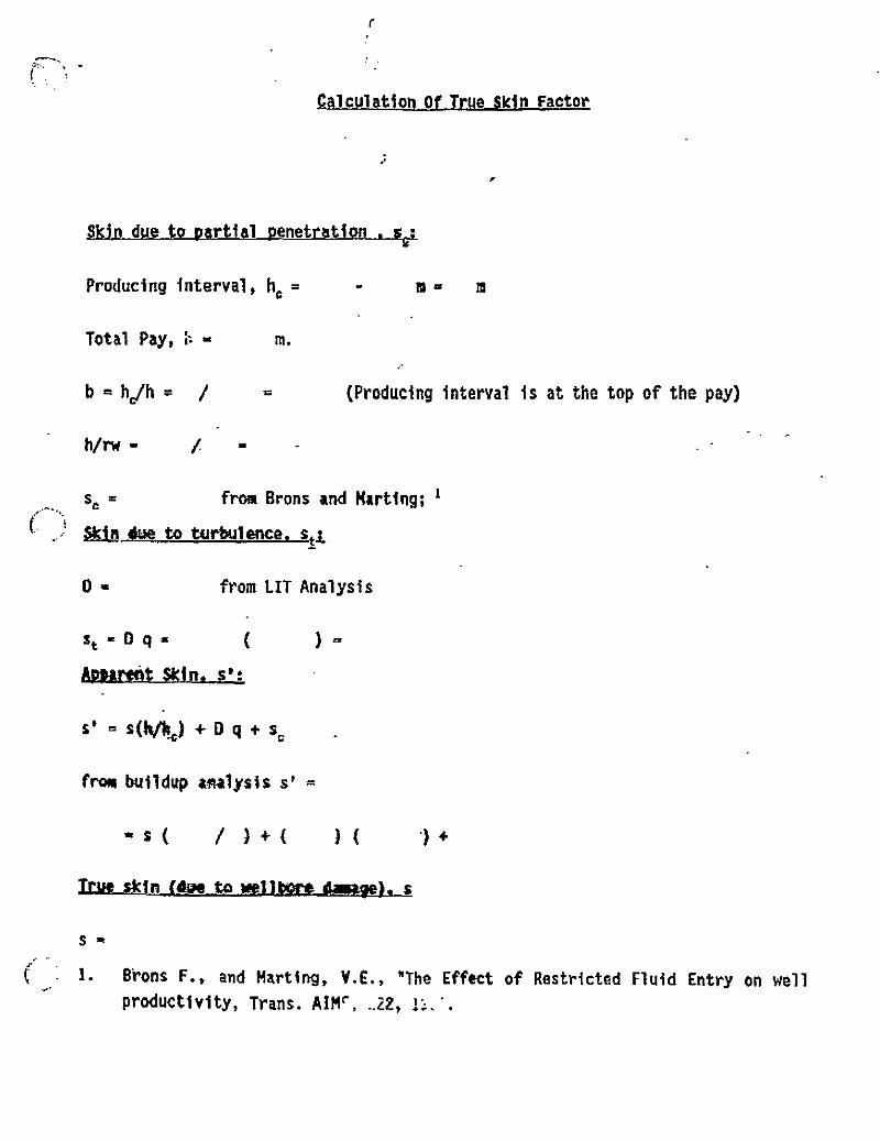
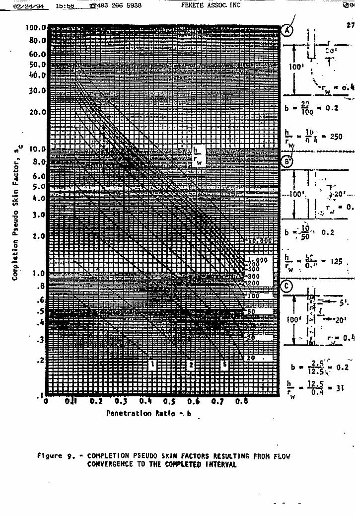

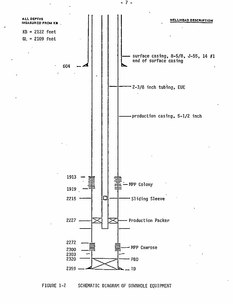
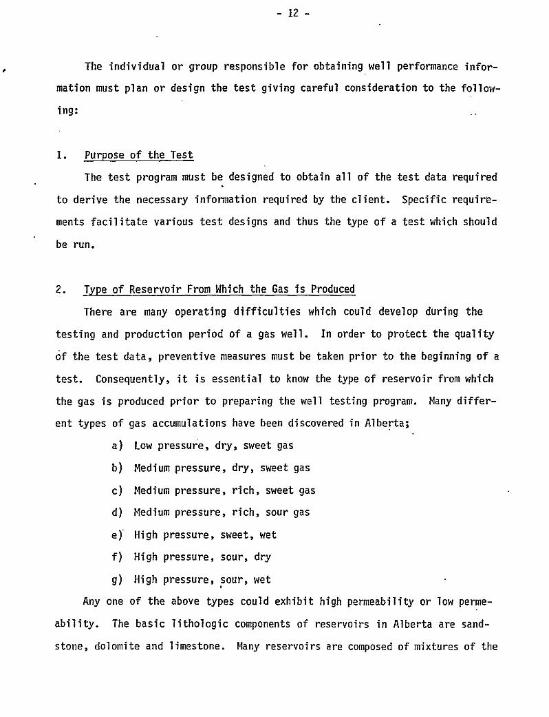
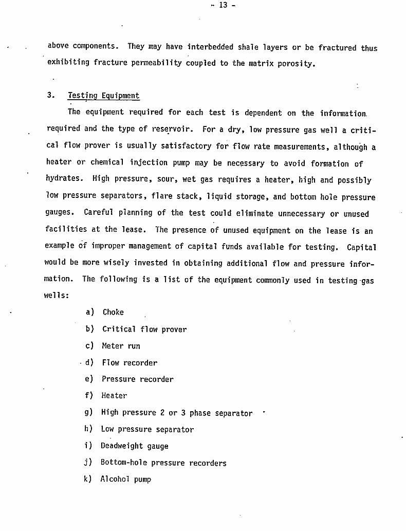
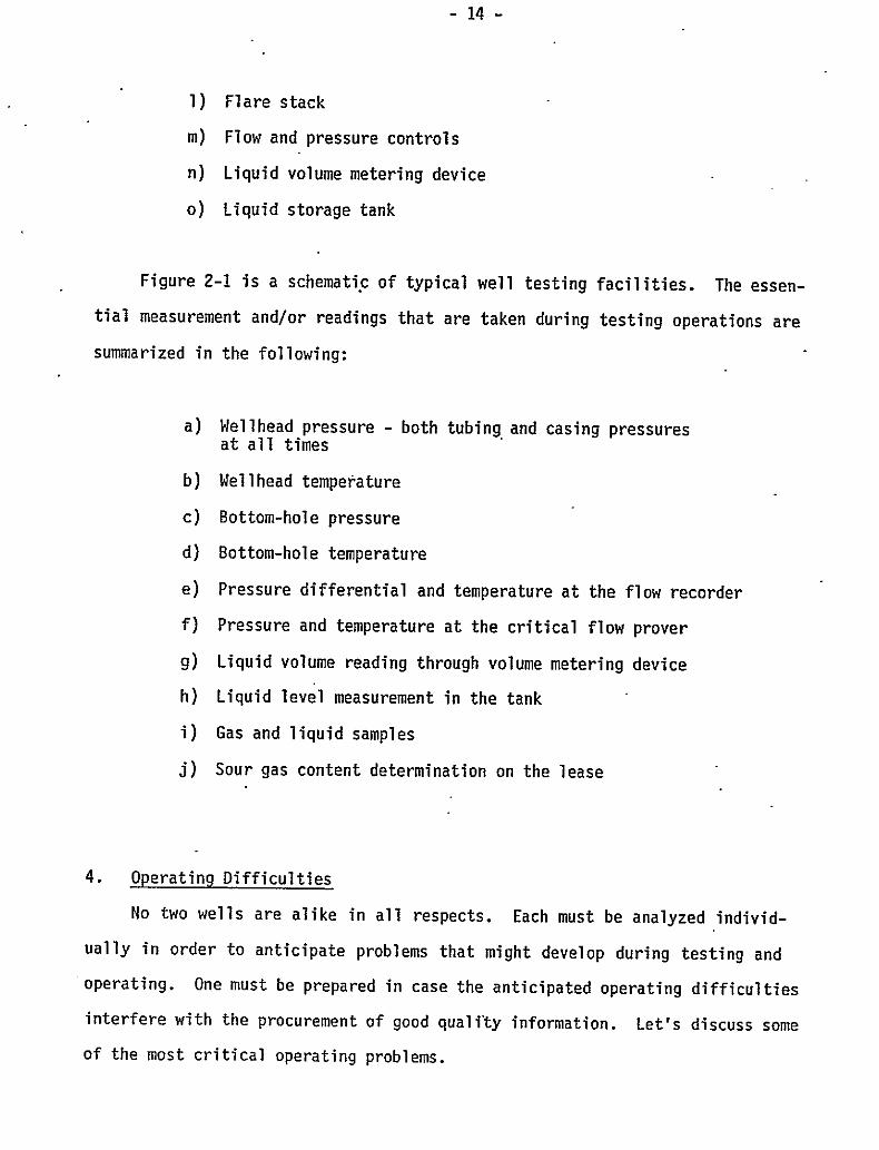
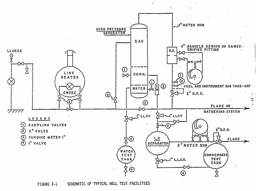
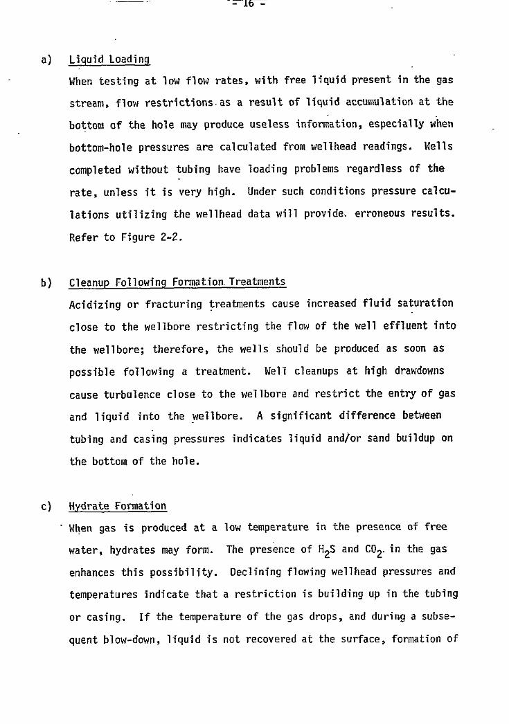
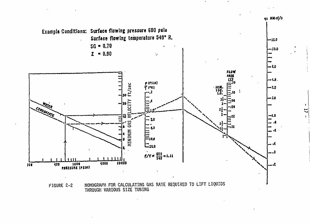
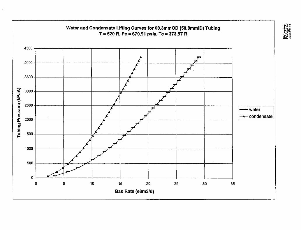
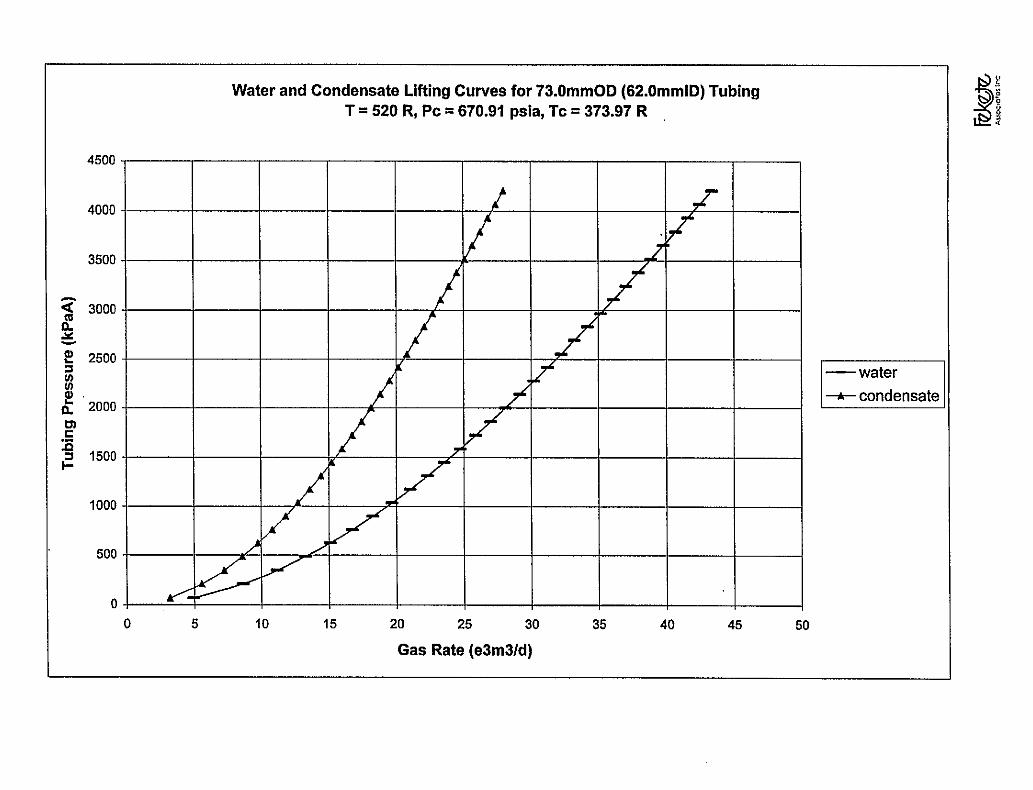
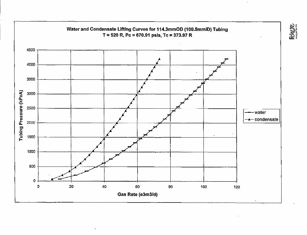
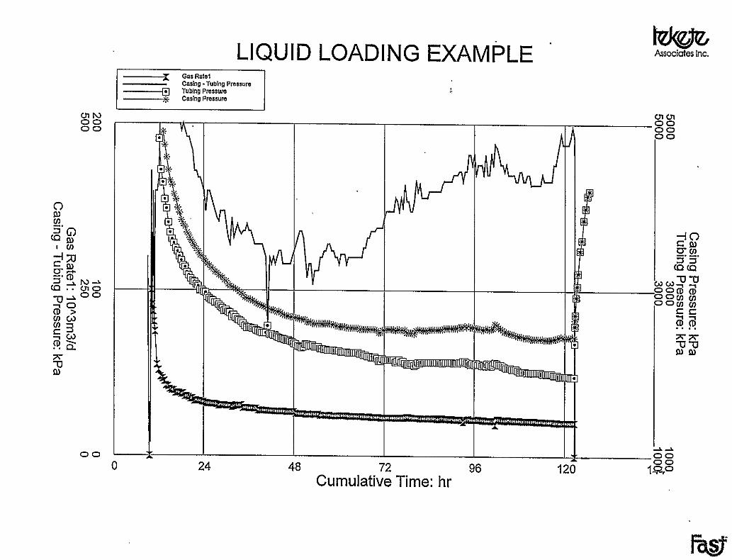
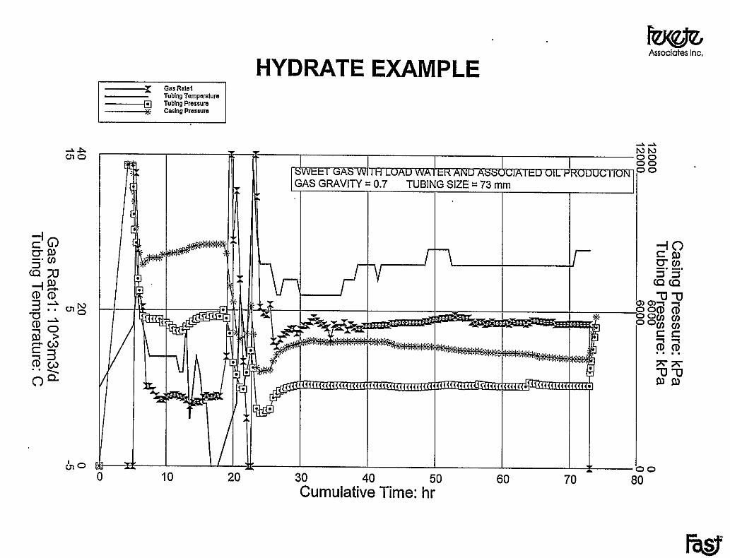
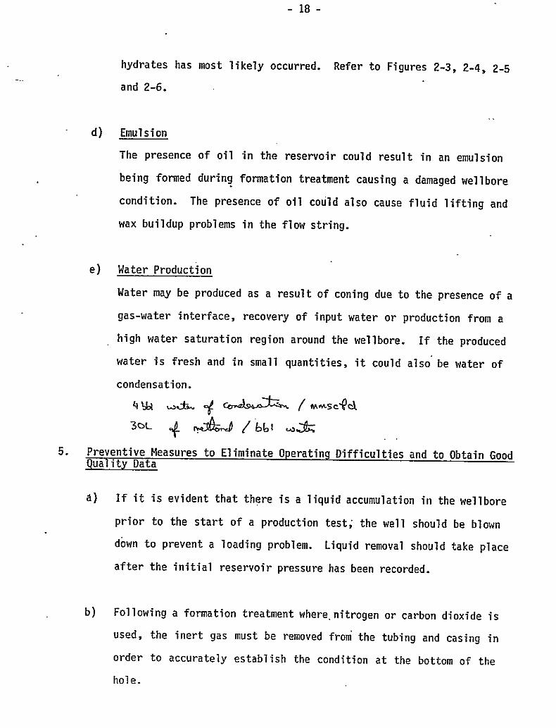
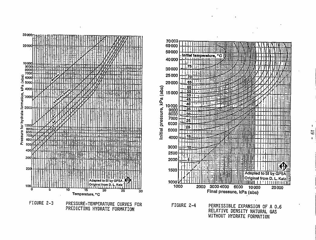
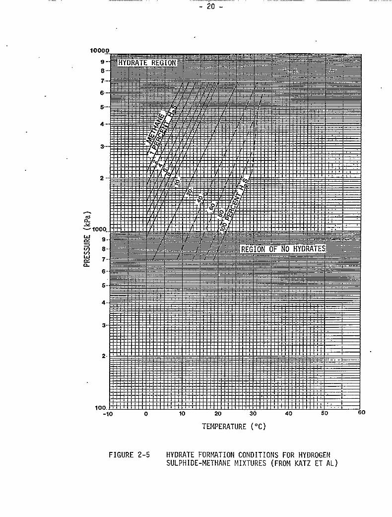
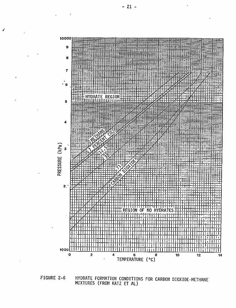

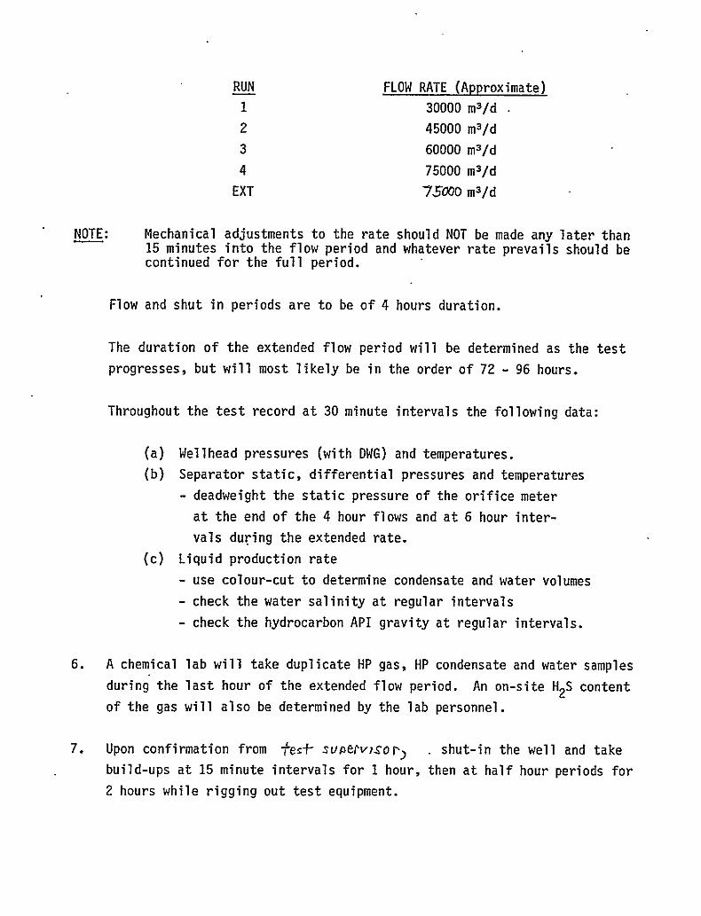
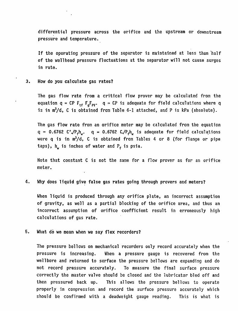
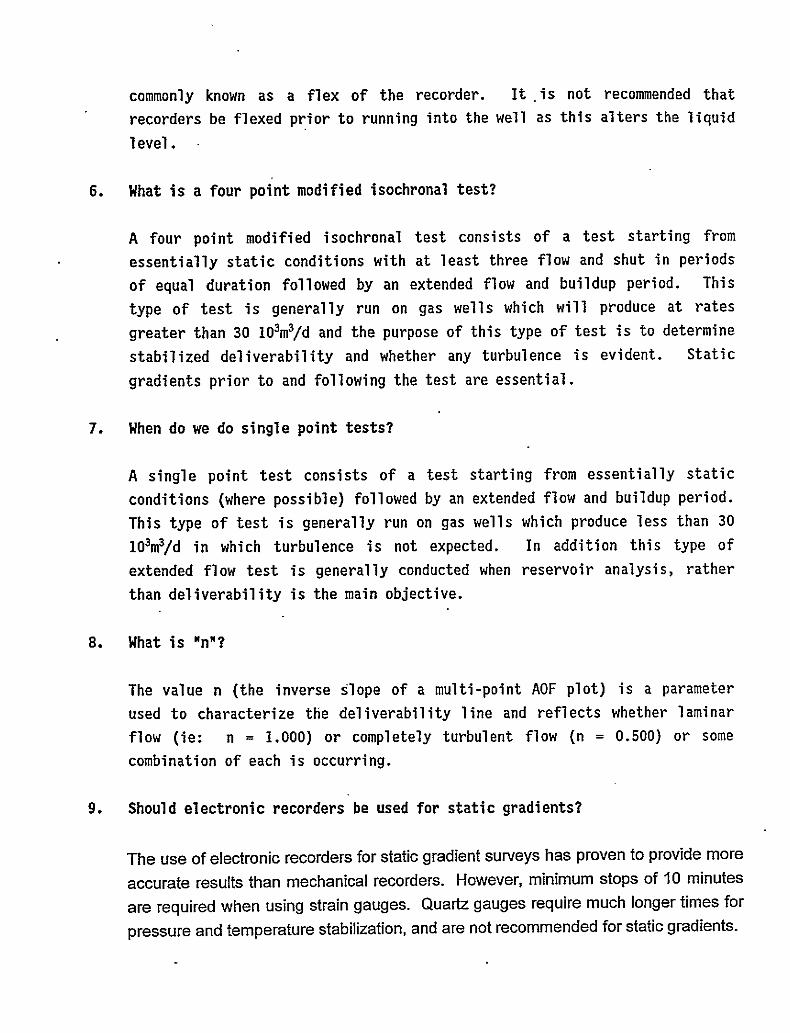
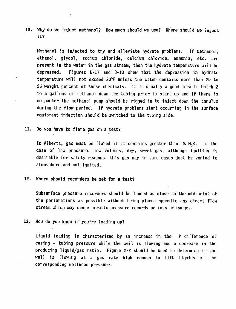
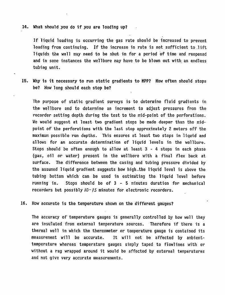
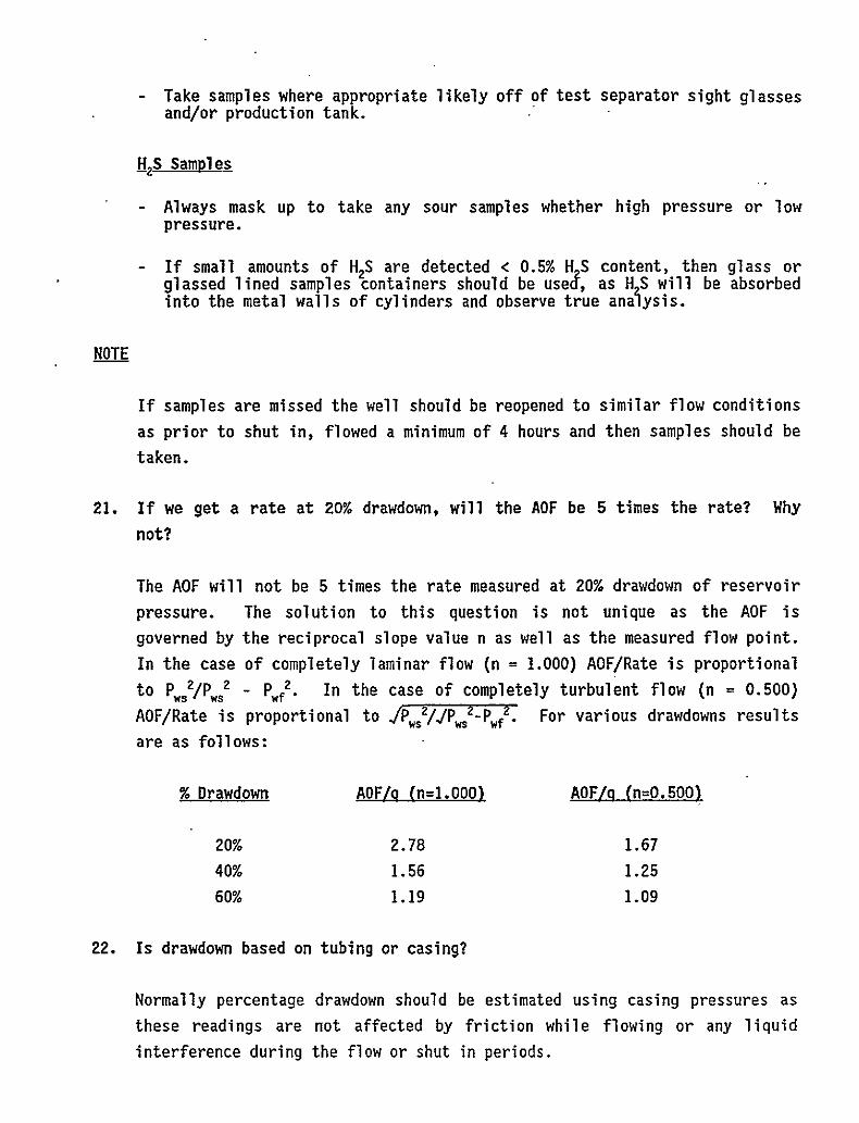
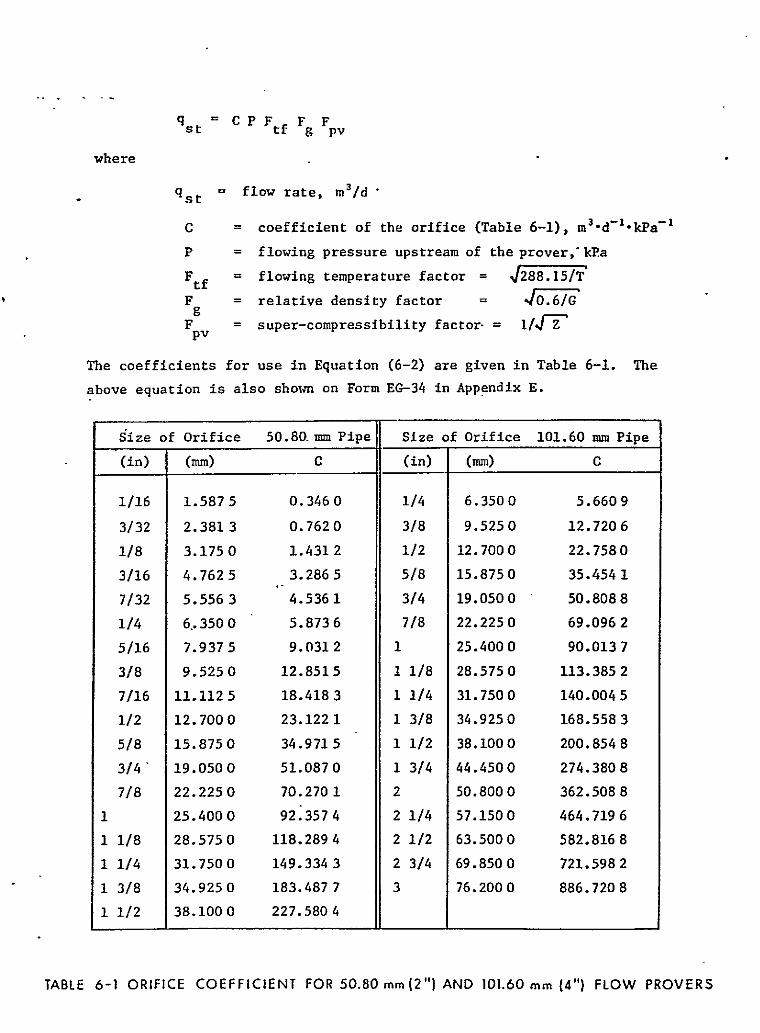
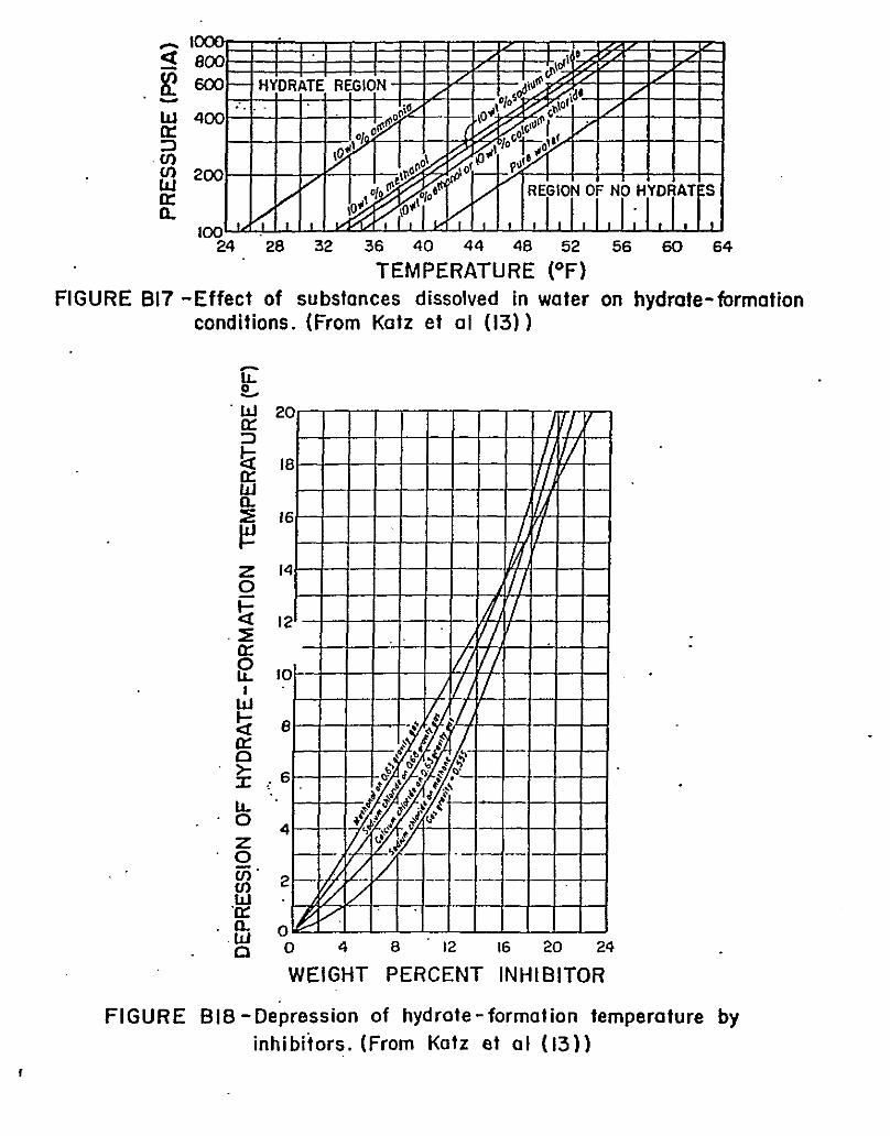

QQuuiizz –– SSeeccttiioonn 11 NNaammee………………………………………………..
11.. GGiivvee FFIIVVEE rreeaassoonnss ffoorr tteessttiinngg::
aa..
bb..
cc..
dd..
ee..
22.. WWhhiicchh tteessttss -- TTrraannssiieenntt ((TT)) oorr SSttaabbiilliizzeedd ((SS)) –– hhaavvee tthhee pprriimmaarryy oobbjjeeccttiivvee ooff oobbttaaiinniinngg tthhee ffoolllloowwiinngg iinnffoorrmmaattiioonn::
PPeerrmmeeaabbiilliittyy (( )),, DDaammaaggee (( )),, SSttiimmuullaattiioonn (( )),, HHyyddrrooccaarrbboonnss iinn ppllaaccee (( )),, RReesseerrvvooiirr hheetteerrooggeenneeiittiieess (( )),, DDeelliivveerraabbiilliittyy (( ))
33.. GGiivvee aapppprrooxxiimmaattee ttiimmee dduurraattiioonn ((hhoouurrss)) ffoorr tthhee ffoolllloowwiinngg tteessttss::
DDrraawwddoowwnn----------,, BBuuiilldduupp------------,, DDSSTT ((oonn--llaanndd))------------,, DDSSTT ((ooffffsshhoorree))------------,, RRFFTT------------,, IInntteerrffeerreennccee--------------,, DDeelliivveerraabbiilliittyy--------------,,
44.. WWhhiicchh iiss tthhee bbeetttteerr ttyyppee ooff tteesstt :: PPuullssee oorr iinntteerrffeerreennccee.. WWhhyy??
55.. NNaammee tthhee ttwwoo tteessttss tthhaatt ccaann bbee uusseedd ttoo ddeetteerrmmiinnee ppoorroossiittyy.. --------------------------------,, ------------------------------------
66.. IIff yyoouu hhaadd vveerryy lliimmiitteedd ffuunnddiinngg aanndd ccoouulldd oonnllyy ccoonndduucctt oonnee tteesstt,, wwhhiicchh tteesstt wwoouulldd yyoouu cchhoooossee,, aanndd wwhhyy??
77.. DDuurriinngg tthhee ffiirrsstt wweeeekk ooff pprroodduuccttiioonn,, WWeellll AA pprroodduucceess @@11000000 bbooppdd wwhheerreeaass WWeellll BB pprroodduucceess @@ 22000000 bbooppdd.. GGiivvee tthhrreeee rreeaassoonnss ffoorr tthhee ddiiffffeerreennccee::
aa..
bb..
cc..
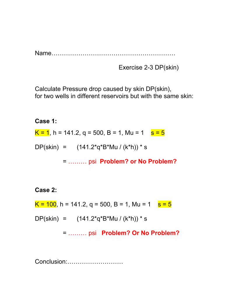
Name…………………………………………………… Exercise 2-3 DP(skin) Calculate Pressure drop caused by skin DP(skin), for two wells in different reservoirs but with the same skin:
Case 1:
K = 1, h = 141.2, q = 500, B = 1, Mu = 1 s = 5 DP(skin) = (141.2*q*B*Mu / (k*h)) * s
= ……… psi Problem? or No Problem?
Case 2: K = 100, h = 141.2, q = 500, B = 1, Mu = 1 s = 5 DP(skin) = (141.2*q*B*Mu / (k*h)) * s
= ……… psi Problem? Or No Problem?
Conclusion:………………………
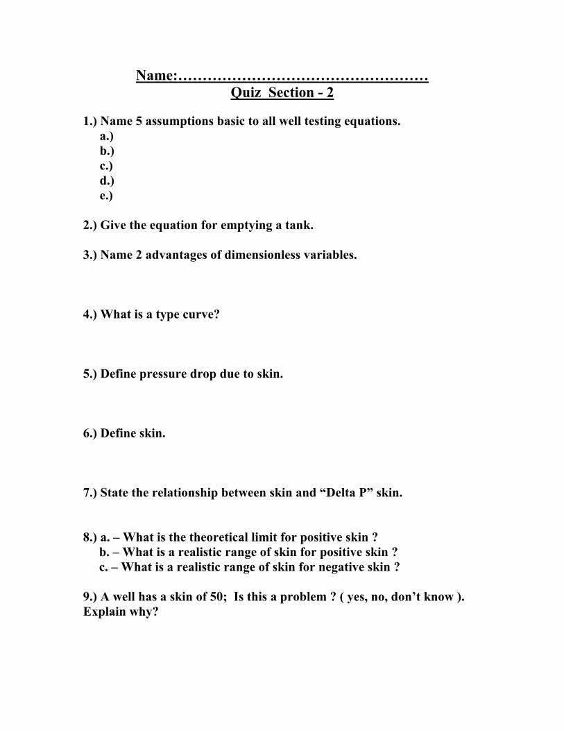
Name:…………………………………………… Quiz Section - 2
1.) Name 5 assumptions basic to all well testing equations.
a.) b.) c.) d.) e.)
2.) Give the equation for emptying a tank. 3.) Name 2 advantages of dimensionless variables. 4.) What is a type curve? 5.) Define pressure drop due to skin. 6.) Define skin. 7.) State the relationship between skin and “Delta P” skin. 8.) a. – What is the theoretical limit for positive skin ? b. – What is a realistic range of skin for positive skin ? c. – What is a realistic range of skin for negative skin ? 9.) A well has a skin of 50; Is this a problem ? ( yes, no, don’t know ). Explain why?
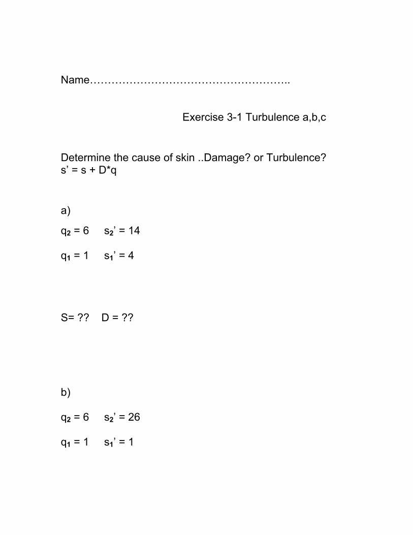
Name………………………………………………..
Exercise 3-1 Turbulence a,b,c
Determine the cause of skin ..Damage? or Turbulence? s’ = s + D*q
a)
q2 = 6 s2’ = 14 q1 = 1 s1’ = 4 S= ?? D = ?? b) q2 = 6 s2’ = 26 q1 = 1 s1’ = 1
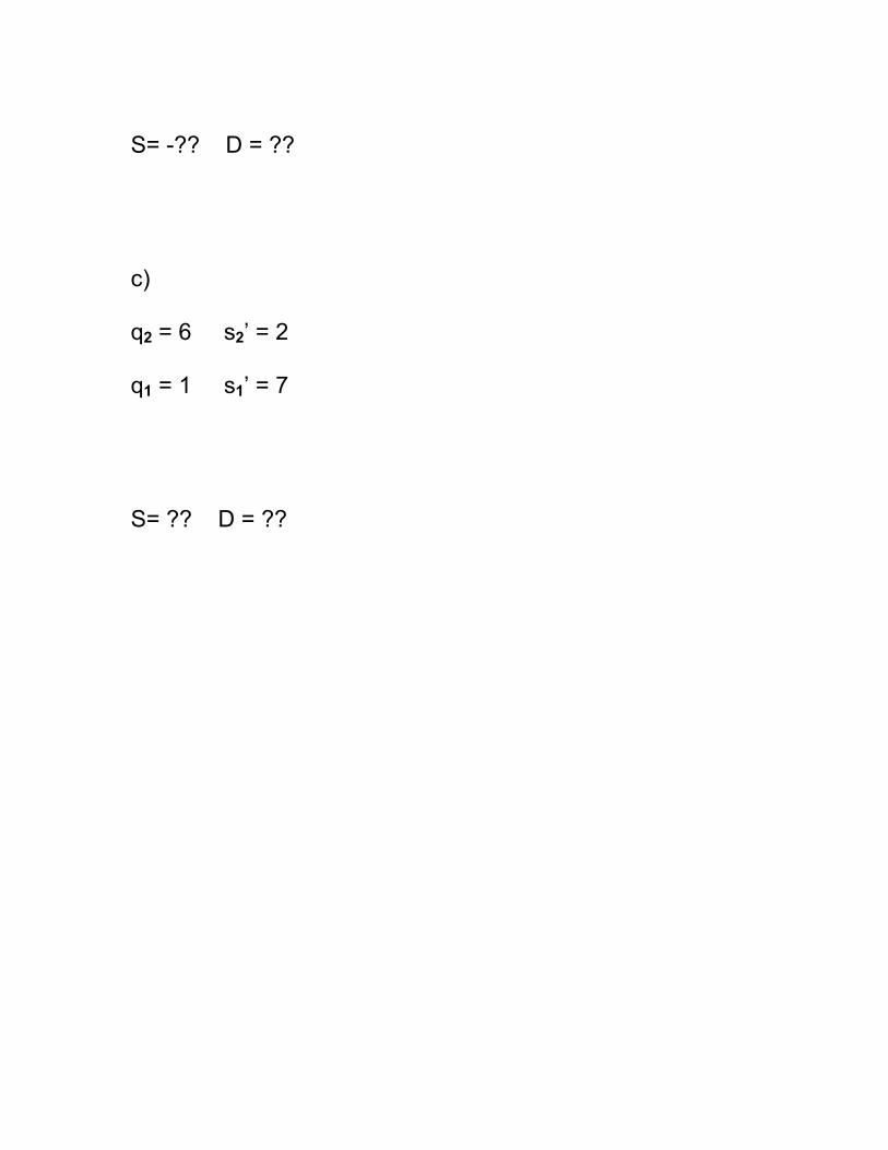
S= -?? D = ?? c) q2 = 6 s2’ = 2 q1 = 1 s1’ = 7 S= ?? D = ??
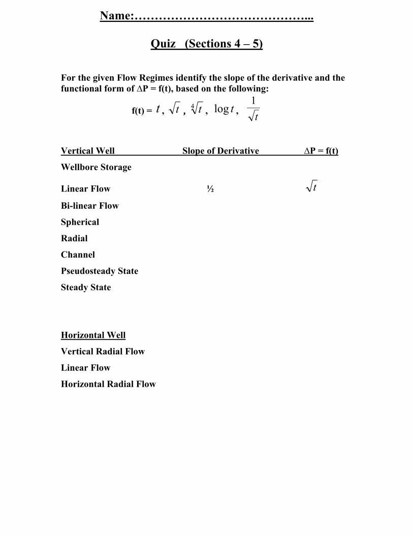
Name:……………………………………...
Quiz (Sections 4 – 5) For the given Flow Regimes identify the slope of the derivative and the functional form of ∆P = f(t), based on the following:
f(t) = t , t , 4 t , tlog , t1
Vertical Well Slope of Derivative ∆P = f(t)
Wellbore Storage
Linear Flow ½ t
Bi-linear Flow
Spherical
Radial
Channel
Pseudosteady State
Steady State
Horizontal Well
Vertical Radial Flow
Linear Flow
Horizontal Radial Flow
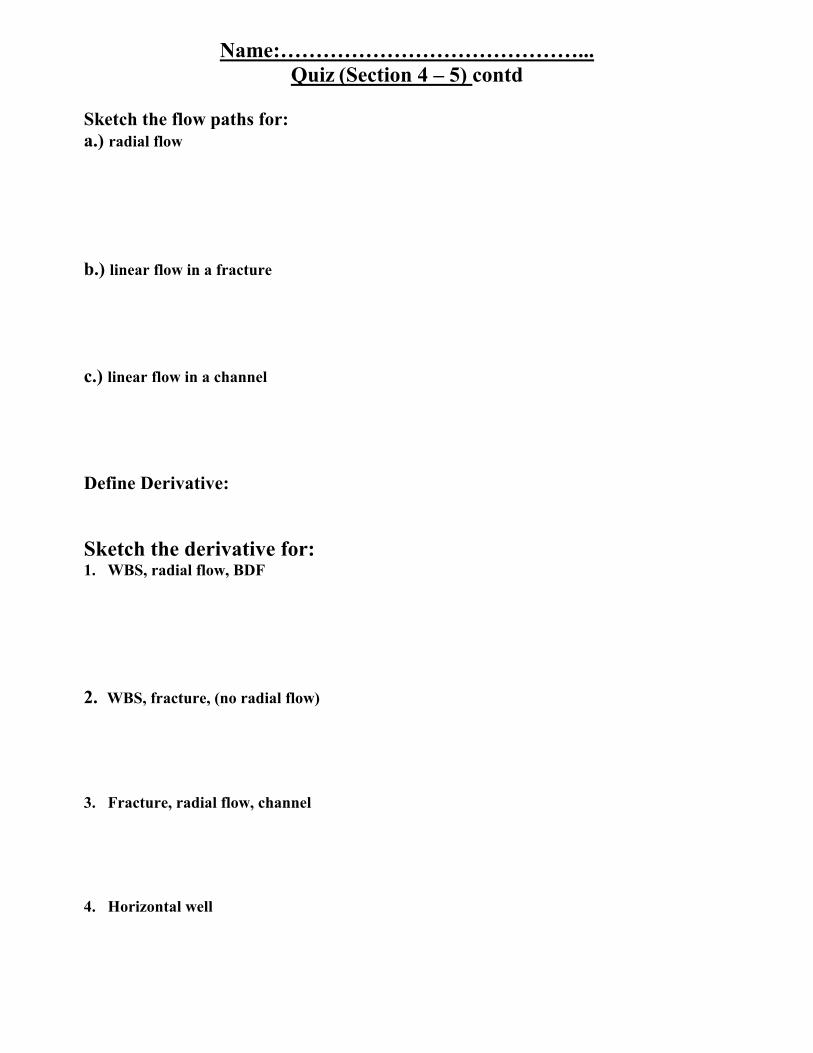
Name:……………………………………...
Quiz (Section 4 – 5) contd
Sketch the flow paths for: a.) radial flow b.) linear flow in a fracture c.) linear flow in a channel Define Derivative: Sketch the derivative for: 1. WBS, radial flow, BDF 2. WBS, fracture, (no radial flow) 3. Fracture, radial flow, channel
4. Horizontal well
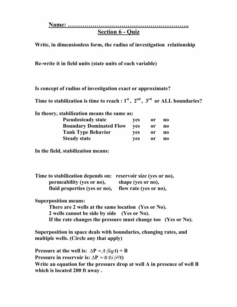
Name: ………………………………………………….. Section 6 - Quiz
Write, in dimensionless form, the radius of investigation relationship Re-write it in field units (state units of each variable) Is concept of radius of investigation exact or approximate? Time to stabilization is time to reach : 1st , 2nd , 3rd or ALL boundaries? In theory, stabilization means the same as:
Pseudosteady state yes or no Boundary Dominated Flow yes or no
Tank Type Behavior yes or no Steady state yes or no In the field, stabilization means: Time to stabilization depends on: reservoir size (yes or no),
permeability (yes or no), shape (yes or no), fluid properties (yes or no), flow rate (yes or no), Superposition means:
There are 2 wells at the same location (Yes or No). 2 wells cannot be side by side (Yes or No).
If the rate changes the pressure must change too (Yes or No). Superposition in space deals with boundaries, changing rates, and multiple wells. (Circle any that apply) Pressure at the well is: ∆P = A (log t) + B Pressure in reservoir is: ∆P = B Ei (r2/t) Write an equation for the pressure drop at well A in presence of well B which is located 200 ft away .
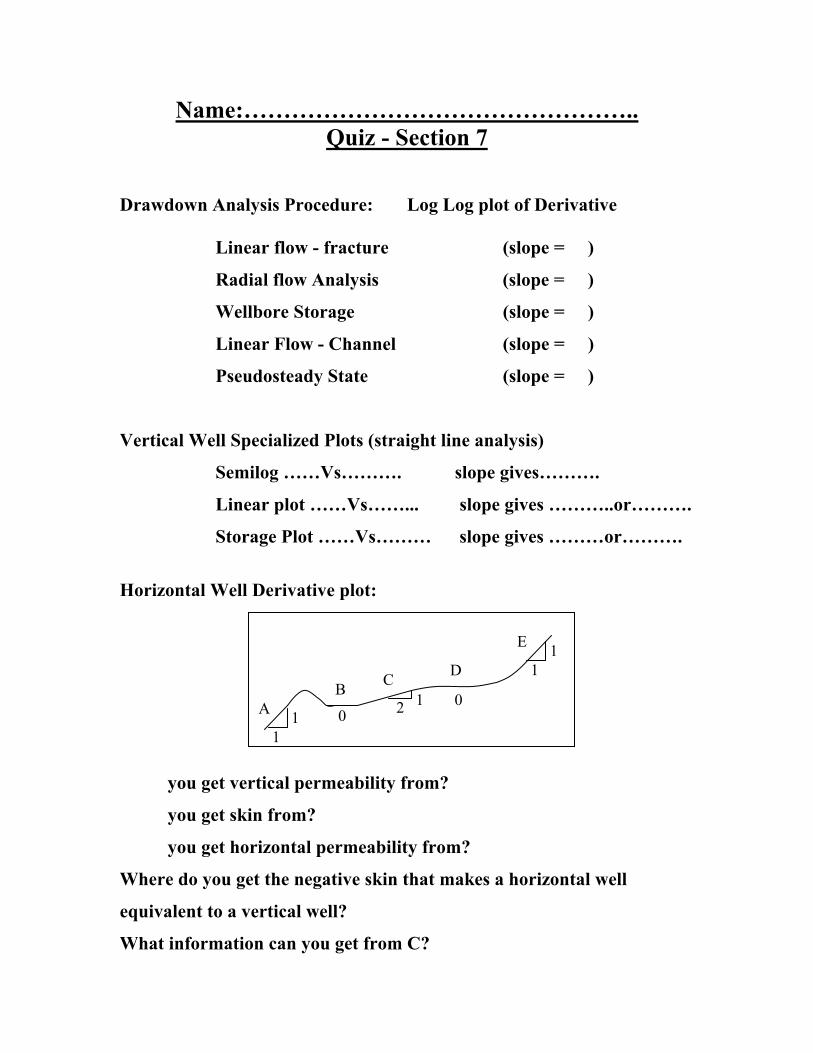
Name:………………………………………….. Quiz - Section 7
Drawdown Analysis Procedure: Log Log plot of Derivative
Linear flow - fracture (slope = )
Radial flow Analysis (slope = )
Wellbore Storage (slope = )
Linear Flow - Channel (slope = )
Pseudosteady State (slope = )
Vertical Well Specialized Plots (straight line analysis)
Semilog ……Vs………. slope gives……….
Linear plot ……Vs……... slope gives ………..or……….
Storage Plot ……Vs……… slope gives ………or……….
Horizontal Well Derivative plot: you get vertical permeability from?
you get skin from?
you get horizontal permeability from?
Where do you get the negative skin that makes a horizontal well
equivalent to a vertical well?
What information can you get from C?
2 1 0
11
1 1
0A B C D
E
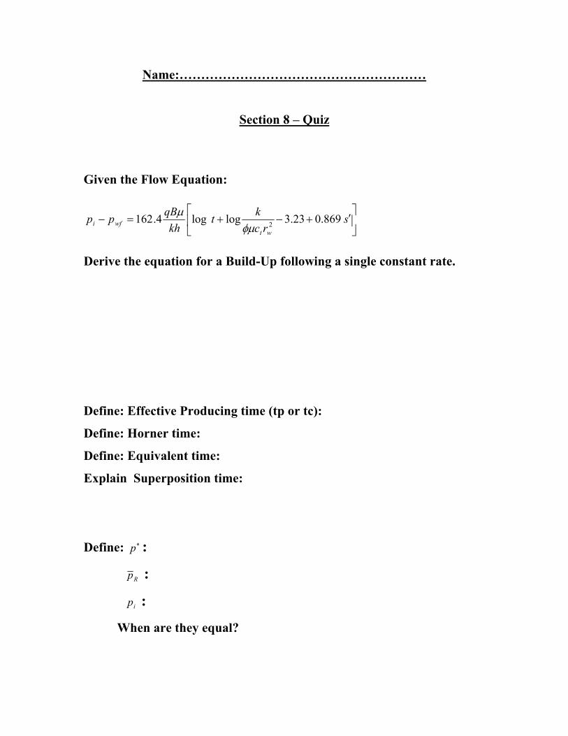
Name:…………………………………………………
Section 8 – Quiz
Given the Flow Equation:
′+−+=− s
rckt
khqBpp
wtwfi 869.023.3loglog4.162 2φµ
µ
Derive the equation for a Build-Up following a single constant rate.
Define: Effective Producing time (tp or tc):
Define: Horner time:
Define: Equivalent time:
Explain Superposition time:
Define: ∗p :
Rp :
ip :
When are they equal?

Name:…………………………………………………
Section 8 – Quiz contd.
How are buildup and fall-off analysis related?
Which part of buildup test data is used to calculate skin?
What is a Horner plot?
What is an M.D.H. plot?
When is it appropriate to use one or the other?
What are M.B.H. plots?

Name:…………………………………………… Quiz Section - 9
Define the PPD. What is it used for? How does it differ from derivative? Why are static gradients conducted? When should they be conducted? Why do we use bottomhole pressure recorders instead of wellhead recorders? Name two things that can cause an increase in the PPD.
If a Horner plot has the shape shown above, how can you tell whether this is a multilayered reservoir effect or a wellbore dynamics effect?
If a Derivative plot has the shape shown above, how can you tell whether this is a dual porosity reservoir or a wellbore dynamics effect?

Name:………………………………………………….. Quiz Section 10
Write down the simplified AOF equation: What are the limits on n, and what do they represent? A modified Isochronal test should have 3 sets of information shown on the plot. Name them: If it takes too long to reach stabilization, what are the various options? Discuss whether an AOF test is valid throughout the life of a well: Write the LIT equation: If there are no wellbore problems, what fraction of sandface AOF is the wellhead AOF? Why do we measure both wellhead and sandface pressures during a test? The field tester says “the rate stabilized after 6 hours”. The well test analyst says, “It takes 6 months to stabilize”. Discuss the above statements: