publ0055:introductiontoquantitativemethods …...example:christianityandvotechoiceingermany 0 20 40...
TRANSCRIPT

PUBL0055: Introduction to Quantitative Methods
Lecture 5: Regression (Specification)
Jack Blumenau and Benjamin Lauderdale
1 / 54

Midterm

Midterm Assessment (administrative)
• Midterm will be released at 6pm on November 1st
• Midterm is due at 2pm on November 6th
• All submissions via Turnitin on Moodle
• Late penalties apply
• Word limit penalties apply
• The word limit is 1,000 words. Tables are not included.
• Extenuating circumstances policies apply
2 / 54

Midterm Assessment (content)
• The midterm may cover any material covered in lectures, seminars orhomeworks during the first five weeks of term (including this week)
• Any material in the textbook that we have not covered in lectures orseminars is not examinable
• The midterm will require you to
• demonstrate conceptual understanding of course material• implement various statistical techniques using R• interpret the output of these techniques in substantive terms
3 / 54

Midterm Assessment (presentation)
• You need to write in full sentences, not bullet points.
• You should present output of all statistical tests in a clear andreadable format.
• Do not copy and paste output from R• Do not include screenshots from R• Do use screenreg or make a table in Word
• Answer the question! If you are asked to answer a policy relevantquestion, you should not simply report a difference in means withoutcommenting on the substance.
• You can use R to answer any question where you think it might beuseful.
4 / 54
Motivation
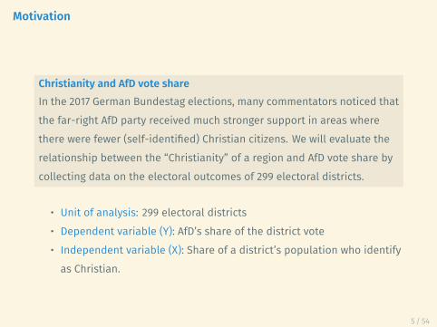
Christianity and AfD vote shareIn the 2017 German Bundestag elections, many commentators noticed thatthe far-right AfD party received much stronger support in areas wherethere were fewer (self-identified) Christian citizens. We will evaluate therelationship between the “Christianity” of a region and AfD vote share bycollecting data on the electoral outcomes of 299 electoral districts.
• Unit of analysis: 299 electoral districts• Dependent variable (Y): AfD’s share of the district vote• Independent variable (X): Share of a district’s population who identifyas Christian.
5 / 54

30 50 70
Christian %
Share of Christians
10 20 30
AfD %
AfD vote share
6 / 54

Christianity and AfD vote share
0 20 40 60 80 100
010
2030
40AfD vote share by Christian Population
Share of population who self−identify as Christian (%)
Afd
sha
re o
f vot
e (%
)
7 / 54

Example: Christianity and vote choice in Germany
• We already know one way to analyse data like this.• We have a continuous dependent variable (AFD Share𝑖)• We have a continuous independent variable (% Christian𝑖)• → bivariate linear regression
• But what if understanding variation in AFD Share𝑖 requires payingattention to more than one variable at a time?
• What if % Christian𝑖 is not the only variable we want to consider?
8 / 54
Lecture Outline
Midterm
Simple/Bivariate Linear Regression
Multiple Linear Regression
…with Categorical Variables
…with Interactions
Multiple and Adjusted R^2
Conclusion
9 / 54
Simple/Bivariate Linear Regression

Example: Christianity and vote choice in Germany
0 20 40 60 80 100
010
2030
40AfD vote share by Christian Population
Share of population who self−identify as Christian (%)
Afd
sha
re o
f vot
e (%
)
10 / 54

Example: Christianity and vote choice in Germany
#### Call:## lm(formula = AfD ~ christian, data = results)#### Residuals:## Min 1Q Median 3Q Max## -11.5059 -2.6182 -0.4376 2.3283 19.5871#### Coefficients:## Estimate Std. Error t value Pr(>|t|)## (Intercept) 21.28552 0.76182 27.94 <2e-16 ***## christian -0.15582 0.01213 -12.84 <2e-16 ***## ---## Signif. codes: 0 '***' 0.001 '**' 0.01 '*' 0.05 '.' 0.1 ' ' 1#### Residual standard error: 4.38 on 297 degrees of freedom## Multiple R-squared: 0.3571, Adjusted R-squared: 0.3549## F-statistic: 165 on 1 and 297 DF, p-value: < 2.2e-16
11 / 54

Example: Christianity and vote choice in Germany
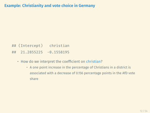
## (Intercept) christian## 21.2855225 -0.1558195
• How do we interpret the intercept?• The expected vote percentage for the AfD in a district that has noChristians is predicted to be 21.3%.
12 / 54
Example: Christianity and vote choice in Germany
## (Intercept) christian## 21.2855225 -0.1558195
• How do we interpret the coefficient on christian?• A one point increase in the percentage of Christians in a district isassociated with a decrease of 0.156 percentage points in the AfD voteshare
12 / 54
Example: Christianity and vote choice in Germany
## (Intercept) christian## 21.2855225 -0.1558195
• Are we happy to conclude that higher levels of Christianity in a districtlead to lower levels of AfD vote?
12 / 54

Causality and Regression
• Are we happy to conclude that higher levels of Christianity in a districtlead to lower levels of AfD vote?
• The language “lead to” makes this sound like a causal relationship.• We have done nothing to justify such a claim!• Question: Why not?
• We can be happy to conclude that the German districts that hadhigher proportions of Christians tended to have lower AfD support
• We cannot conclude anything about why this is the case on the basis ofthis simple linear regression.
13 / 54
This lecture and next lecture
• This lecture we will explore the ways multiple linear regression can beused to describe variation in an outcome (like AfD vote share) usingmore than one explanatory variable.
• Multiple regression specification for prediction
• Next lecture we will consider how to use Multiple Linear Regression totry establish causal claims about specific explanatory variables.
• Multiple regression specification for causal inference
14 / 54

Multiple Linear Regression

Example: Christianity and vote choice in Germany
0 20 40 60 80 100
010
2030
40AfD vote share by Christian Population
Share of population who self−identify as Christian (%)
Afd
sha
re o
f vot
e (%
)
15 / 54

Example: Christianity and vote choice in Germany
0 20 40 60 80 100
010
2030
40AfD vote share by Christian Population
Share of population who self−identify as Christian (%)
Afd
sha
re o
f vot
e (%
)
Former East GermanyFormer West Germany
16 / 54

Example: Christianity and vote choice in Germany
0 20 40 60 80 100
010
2030
40AfD vote share by Christian Population
Share of population who self−identify as Christian (%)
Afd
sha
re o
f vot
e (%
)
Former East GermanyFormer West Germany
17 / 54
Example: Christianity and vote choice in Germany
0 20 40 60 80 100
010
2030
40AfD vote share by Christian Population
Share of population who self−identify as Christian (%)
Afd
sha
re o
f vot
e (%
)
Former East GermanyFormer West Germany
18 / 54

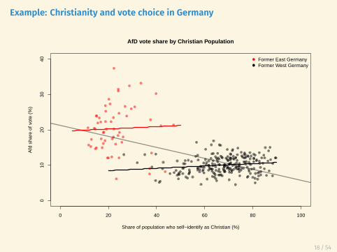
Example: Christianity and vote choice in Germany
• AfD vote share is very different in East and West
• The Christian % is also very different in East and West
• If we estimate the relationship between Christianity and AfD votewithin East and West Germany things look very different!
19 / 54

Moving beyond one variable
• Multiple regression provides a framework for describing variation inan outcome variable using more than one variable at once
• 𝑌 : AfD vote share• 𝑋1: Christian %• 𝑋2: Former East/West
20 / 54

Multiple Regression
The multiple regression model is:
𝑌𝑖 = 𝛼 + 𝛽1𝑋1 + 𝛽2𝑋2 + ... + 𝛽𝑘𝑋𝑘 + 𝜖𝑖
• Observations 𝑖 = 1, ..., 𝑛• Y is the dependent variables• 𝑋1, ..., 𝑋𝑘 are k explanatory variables• 𝛼 is the intercept or constant• 𝛽1, ..., 𝛽𝑘 are the coefficients• 𝜖𝑖 is the error term
21 / 54

The Multiple Linear Regression Model
An alternative, but equivalent, statement of the model is given by:
𝐸(𝑌𝑖|𝑋1, 𝑋2, ..., 𝑋𝑘) = 𝛼 + 𝛽1𝑋1 + 𝛽2𝑋2 + ... + 𝛽𝑘𝑋𝑘
• 𝐸(𝑌𝑖|𝑋1, 𝑋2, ..., 𝑋𝑘) represents the conditional expected value ofY, given our X variables
• This formulation makes clear that the linear regression model is amodel for the mean or the expected value of our outcome fordifferent values of our explanatory variables
22 / 54
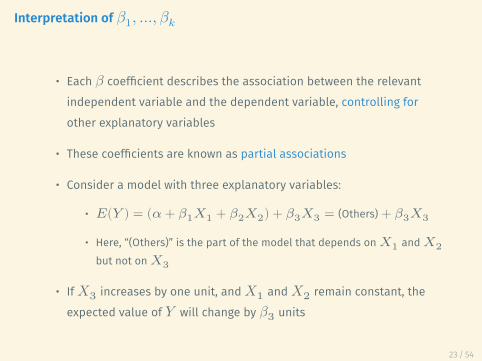
Interpretation of 𝛽1, ..., 𝛽𝑘
• Each 𝛽 coefficient describes the association between the relevantindependent variable and the dependent variable, controlling forother explanatory variables
• These coefficients are known as partial associations
• Consider a model with three explanatory variables:
• 𝐸(𝑌 ) = (𝛼 + 𝛽1𝑋1 + 𝛽2𝑋2) + 𝛽3𝑋3 = (Others) + 𝛽3𝑋3
• Here, “(Others)” is the part of the model that depends on 𝑋1 and 𝑋2but not on 𝑋3
• If 𝑋3 increases by one unit, and 𝑋1 and 𝑋2 remain constant, theexpected value of 𝑌 will change by 𝛽3 units
23 / 54
Interpretation of 𝛽1, ..., 𝛽𝑘
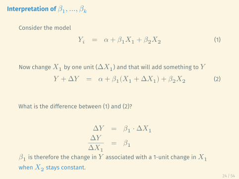
Consider the model
𝑌𝑖 = 𝛼 + 𝛽1𝑋1 + 𝛽2𝑋2 (1)
Now change 𝑋1 by one unit (Δ𝑋1) and that will add something to 𝑌𝑌 + Δ𝑌 = 𝛼 + 𝛽1(𝑋1 + Δ𝑋1) + 𝛽2𝑋2 (2)
What is the difference between (1) and (2)?
Δ𝑌 = 𝛽1 ⋅ Δ𝑋1Δ𝑌
Δ𝑋1= 𝛽1
𝛽1 is therefore the change in 𝑌 associated with a 1-unit change in 𝑋1when 𝑋2 stays constant.
24 / 54
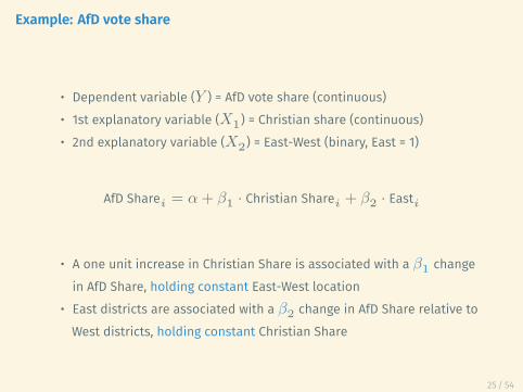
Example: AfD vote share
• Dependent variable (𝑌 ) = AfD vote share (continuous)• 1st explanatory variable (𝑋1) = Christian share (continuous)• 2nd explanatory variable (𝑋2) = East-West (binary, East = 1)
AfD Share𝑖 = 𝛼 + 𝛽1 ⋅ Christian Share𝑖 + 𝛽2 ⋅ East𝑖
• A one unit increase in Christian Share is associated with a 𝛽1 changein AfD Share, holding constant East-West location
• East districts are associated with a 𝛽2 change in AfD Share relative toWest districts, holding constant Christian Share
25 / 54

Interpretation of 𝛽1, ..., 𝛽𝑘
0 20 40 60 80 100
010
2030
40
AfD vote share by Christian Population
Share of population who self−identify as Christian (%)
Afd
sha
re o
f vot
e (%
)
EastWest
• Let’s “hold constant” ourEast-West explanatory variable
• 𝛽1 describes the slope of thelines within East and Westdistricts
26 / 54
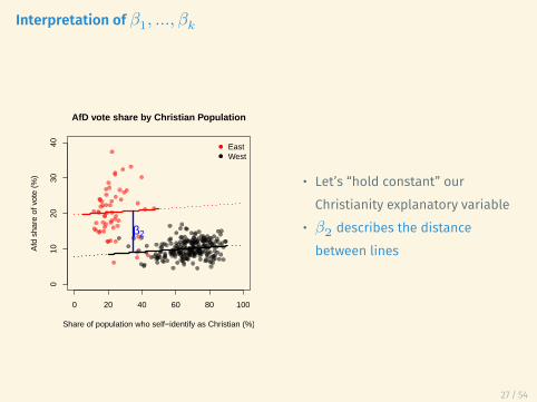
Interpretation of 𝛽1, ..., 𝛽𝑘
0 20 40 60 80 100
010
2030
40
AfD vote share by Christian Population
Share of population who self−identify as Christian (%)
Afd
sha
re o
f vot
e (%
)
EastWest
β2
• Let’s “hold constant” ourChristianity explanatory variable
• 𝛽2 describes the distancebetween lines
27 / 54

Multiple linear regression in R
# our original model with one explanatory variablelinear_model_1 <- lm(AfD ~ christian, data = results)
# our new model, with two explanatory variableslinear_model_2 <- lm(AfD ~ christian + east, data = results)
28 / 54
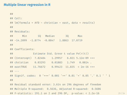
Multiple linear regression in R
#### Call:## lm(formula = AfD ~ christian + east, data = results)#### Residuals:## Min 1Q Median 3Q Max## -14.2099 -1.8774 -0.0847 1.8863 17.0719#### Coefficients:## Estimate Std. Error t value Pr(>|t|)## (Intercept) 7.82484 1.29957 6.021 5.12e-09 ***## christian 0.03293 0.01883 1.749 0.0814 .## eastTRUE 11.76672 0.99423 11.835 < 2e-16 ***## ---## Signif. codes: 0 '***' 0.001 '**' 0.01 '*' 0.05 '.' 0.1 ' ' 1#### Residual standard error: 3.614 on 296 degrees of freedom## Multiple R-squared: 0.5636, Adjusted R-squared: 0.5606## F-statistic: 191.1 on 2 and 296 DF, p-value: < 2.2e-16 29 / 54

Multiple linear regression output
AfD
christian 0.033(0.019)
east 11.767∗
(0.994)
Constant 7.825∗
(1.300)
Observations 299R2 0.564
Note: ∗p<0.05
• A one point increase in theshare of Christians is associatedwith a 0.03 point increase in theAfD share of the vote onaverage, holding constantEast-West location
• East districts are associatedwith 11.8 points higher AfD voteshare on average, holdingconstant the share of Christians
30 / 54

Interpretation of 𝛼
• Last week, the interpretation of 𝛼 was the average value of Y when𝑋 = 0
• Now we have more than one X, 𝛼 represents the average value of 𝑌when all X variables are equal to zero
• As we add more and more independent variables, 𝛼 becomes lesslikely to be a quantity that has a substantively interestinginterpretation
31 / 54

Interpretation of 𝛼
0 20 40 60 80 100
010
2030
40
AfD vote share by Christian Population
Share of population who self−identify as Christian (%)
Afd
sha
re o
f vot
e (%
)
EastWest
β0
• Remember, our X variable forEast-West is equal to 1 for Eastdistricts and 0 for West districts
• 𝛼 is therefore the point atwhich the black line intersectsthe Y-axis
32 / 54
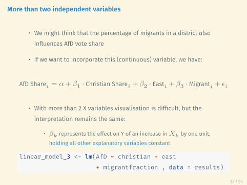
More than two independent variables
• We might think that the percentage of migrants in a district alsoinfluences AfD vote share
• If we want to incorporate this (continuous) variable, we have:
AfD Share𝑖 = 𝛼 + 𝛽1 ⋅ Christian Share𝑖 + 𝛽2 ⋅ East𝑖 + 𝛽3 ⋅ Migrant𝑖 + 𝜖𝑖
• With more than 2 X variables visualisation is difficult, but theinterpretation remains the same:
• 𝛽𝑘 represents the effect on Y of an increase in 𝑋𝑘 by one unit,holding all other explanatory variables constant
linear_model_3 <- lm(AfD ~ christian + east+ migrantfraction , data = results)
33 / 54
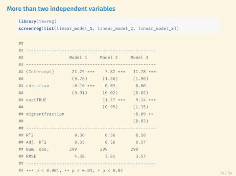
More than two independent variableslibrary(texreg)screenreg(list(linear_model_1, linear_model_2, linear_model_3))
#### ===================================================## Model 1 Model 2 Model 3## ---------------------------------------------------## (Intercept) 21.29 *** 7.82 *** 11.78 ***## (0.76) (1.30) (1.90)## christian -0.16 *** 0.03 0.00## (0.01) (0.02) (0.02)## eastTRUE 11.77 *** 9.14 ***## (0.99) (1.35)## migrantfraction -0.09 **## (0.03)## ---------------------------------------------------## R^2 0.36 0.56 0.58## Adj. R^2 0.35 0.56 0.57## Num. obs. 299 299 299## RMSE 4.38 3.61 3.57## ===================================================## *** p < 0.001, ** p < 0.01, * p < 0.05 34 / 54

Fitted values
As before, we can calculate fitted values for our model:
• The fitted values ( 𝑌 ) are:
𝑌𝑖 = 𝛼 + 𝛽1𝑋1𝑖 + 𝛽2𝑋2𝑖 + ... + 𝛽𝑘𝑋𝑘𝑖
• Interpretation: The fitted values tell us the best guess for Y for specificvalues of 𝑋1, 𝑋2, ..., 𝑋𝑘
35 / 54
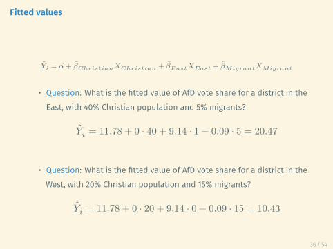
Fitted values
𝑌𝑖 = �� + 𝛽𝐶ℎ𝑟𝑖𝑠𝑡𝑖𝑎𝑛𝑋𝐶ℎ𝑟𝑖𝑠𝑡𝑖𝑎𝑛 + 𝛽𝐸𝑎𝑠𝑡𝑋𝐸𝑎𝑠𝑡 + 𝛽𝑀𝑖𝑔𝑟𝑎𝑛𝑡𝑋𝑀𝑖𝑔𝑟𝑎𝑛𝑡
• Question: What is the fitted value of AfD vote share for a district in theEast, with 40% Christian population and 5% migrants?
𝑌𝑖 = 11.78 + 0 ⋅ 40 + 9.14 ⋅ 1 − 0.09 ⋅ 5 = 20.47
• Question: What is the fitted value of AfD vote share for a district in theWest, with 20% Christian population and 15% migrants?
𝑌𝑖 = 11.78 + 0 ⋅ 20 + 9.14 ⋅ 0 − 0.09 ⋅ 15 = 10.43
36 / 54

Break
37 / 54

…with Categorical Variables

Categorical Variables and “Qualitative Information”
• We have already seen that we can incorporate qualitative informationby using dummy variables
• Our “East” variable indicated whether a given district was located in(old) East Germany
• We can also include information for many groups
• The 299 districts in Germany are clustered in 16 “regions”
• We do so by including a set of dummy variables for all groups(regions) except for one
38 / 54

Categorical Variables
• Include dummy variables for all but one category
• The category without a dummy is the reference or baseline category
• The coefficient of the category is the expected difference in Y betweenthe category and the baseline
• The choice of baseline is arbitrary: the model is identical insubstantive terms
39 / 54

Categorical Variables
• Example set of dummy variables for a categorical variable with levelsof England, Scotland, Wales, and N. Ireland
• The reference category is England:
𝑋𝑆 𝑋𝑊 𝑋𝑁𝐼Wales 0 1 0England 0 0 0Scotland 1 0 0N. Ireland 0 0 1N. Ireland 0 0 1England 0 0 0⋮ ⋮ ⋮ ⋮
• R will automatically convert any factor variable into a set of dummies,and will choose a baseline category 40 / 54

Categorical Variable Example
We will use the region variable from our data:
#### BB BE BW BY HB HE HH MV NI NW RP SH SL SN ST TH## 10 12 38 46 2 22 6 6 30 64 15 11 4 16 9 8
This shows the number of constituencies in each region in the data.
We can estimate a model with a categorical variable as before:linear_model_4 <- lm(AfD ~ christian + region , data = results)
41 / 54

Categorical Variable Example
## Estimate Std. Error t value Pr(>|t|)## (Intercept) 19.38519398 0.98617499 19.6569516 8.906315e-55## christian 0.01948636 0.01956459 0.9960014 3.201033e-01## regionBE -7.88621573 1.23122444 -6.4051813 6.268269e-10## regionBW -9.19481347 1.39715459 -6.5810996 2.269137e-10## regionBY -9.99382116 1.46489653 -6.8222028 5.466454e-11## regionHB -10.76355393 2.29222915 -4.6956710 4.154088e-06## regionHE -9.78162918 1.38520152 -7.0615207 1.286179e-11## regionHH -11.89533599 1.52194233 -7.8158914 1.089623e-13## regionMV -1.60037325 1.47391164 -1.0858000 2.784948e-01## regionNI -11.90378488 1.36936299 -8.6929360 2.951986e-16## regionNW -11.25031787 1.34611890 -8.3575960 2.953719e-15## regionRP -10.56147953 1.58461659 -6.6650063 1.388249e-10## regionSH -13.04309714 1.45041829 -8.9926453 3.612896e-17## regionSL -11.64505844 2.06876178 -5.6289992 4.374645e-08## regionSN 6.40523554 1.15243488 5.5580021 6.321840e-08## regionST -1.26241031 1.31281745 -0.9616038 3.370724e-01## regionTH 2.49520321 1.36963016 1.8218080 6.954336e-02
• In our data “region” is a categorical (factor) variable• Brandenburg (BB) is the baseline category
42 / 54

Categorical Variable Example
## Estimate Std. Error t value Pr(>|t|)## (Intercept) 19.38519398 0.98617499 19.6569516 8.906315e-55## christian 0.01948636 0.01956459 0.9960014 3.201033e-01## regionBE -7.88621573 1.23122444 -6.4051813 6.268269e-10## regionBW -9.19481347 1.39715459 -6.5810996 2.269137e-10## regionBY -9.99382116 1.46489653 -6.8222028 5.466454e-11## regionHB -10.76355393 2.29222915 -4.6956710 4.154088e-06## regionHE -9.78162918 1.38520152 -7.0615207 1.286179e-11## regionHH -11.89533599 1.52194233 -7.8158914 1.089623e-13## regionMV -1.60037325 1.47391164 -1.0858000 2.784948e-01## regionNI -11.90378488 1.36936299 -8.6929360 2.951986e-16## regionNW -11.25031787 1.34611890 -8.3575960 2.953719e-15## regionRP -10.56147953 1.58461659 -6.6650063 1.388249e-10## regionSH -13.04309714 1.45041829 -8.9926453 3.612896e-17## regionSL -11.64505844 2.06876178 -5.6289992 4.374645e-08## regionSN 6.40523554 1.15243488 5.5580021 6.321840e-08## regionST -1.26241031 1.31281745 -0.9616038 3.370724e-01## regionTH 2.49520321 1.36963016 1.8218080 6.954336e-02
• Controlling for the Christian share of the population, the AfD share inBerlin (BE) is 7.9 points lower than in Brandenburg on average
42 / 54

Categorical Variable Example
## Estimate Std. Error t value Pr(>|t|)## (Intercept) 19.38519398 0.98617499 19.6569516 8.906315e-55## christian 0.01948636 0.01956459 0.9960014 3.201033e-01## regionBE -7.88621573 1.23122444 -6.4051813 6.268269e-10## regionBW -9.19481347 1.39715459 -6.5810996 2.269137e-10## regionBY -9.99382116 1.46489653 -6.8222028 5.466454e-11## regionHB -10.76355393 2.29222915 -4.6956710 4.154088e-06## regionHE -9.78162918 1.38520152 -7.0615207 1.286179e-11## regionHH -11.89533599 1.52194233 -7.8158914 1.089623e-13## regionMV -1.60037325 1.47391164 -1.0858000 2.784948e-01## regionNI -11.90378488 1.36936299 -8.6929360 2.951986e-16## regionNW -11.25031787 1.34611890 -8.3575960 2.953719e-15## regionRP -10.56147953 1.58461659 -6.6650063 1.388249e-10## regionSH -13.04309714 1.45041829 -8.9926453 3.612896e-17## regionSL -11.64505844 2.06876178 -5.6289992 4.374645e-08## regionSN 6.40523554 1.15243488 5.5580021 6.321840e-08## regionST -1.26241031 1.31281745 -0.9616038 3.370724e-01## regionTH 2.49520321 1.36963016 1.8218080 6.954336e-02
• Controlling for the Christian share of the population, the AfD share inSachsen (SN) is 6.4 points higher than in Brandenburg on average
42 / 54

…with Interactions

Interactions
InteractionsAn interaction exists between two explanatory variables when therelationship between (either) one of them and the dependent variabledepends on the value of the other.
• We can build this intuition into the linear regression model byincluding the product of two explanatory variables in our model
• We are going to continue on with the same data set, but now focusingon whether the relationship between migrantfraction (𝑋1) andafd (𝑌 ) is different for East and West districts (𝑋2)
43 / 54

Conditional Effects
• The simple model we have been studying assumes ‘constant effects’(i.e. the effect of each 𝑋 does not depend on other 𝑋s)
𝑌𝑖 = 𝛼 + 𝛽1𝑋1𝑖 + 𝛽2𝑋2𝑖
• We can relax the assumption of constant effects by adding theproduct of explanatory variables to a model:
𝑌𝑖 = 𝛼 + 𝛽1𝑋1𝑖 + 𝛽2𝑋2𝑖 + 𝛽3𝑋1𝑖 ⋅ 𝑋2𝑖 + 𝜀𝑖
• In our example, we could run the following models:
AfD = 𝛼 + 𝛽1 ∗ migrant + 𝛽2 ∗ eastAfD = 𝛼 + 𝛽1 ∗ migrant + 𝛽2 ∗ east + 𝛽3 ∗ migrant ⋅ east
44 / 54
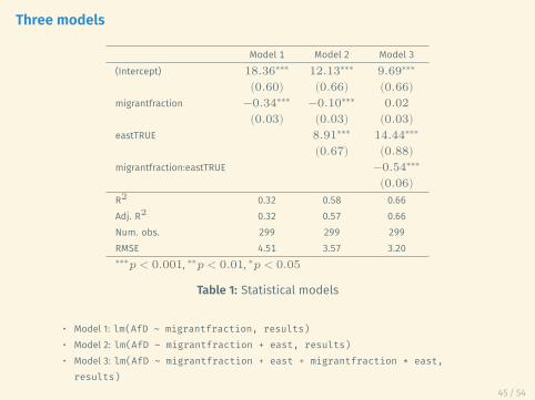
Three models
Model 1 Model 2 Model 3(Intercept) 18.36∗∗∗ 12.13∗∗∗ 9.69∗∗∗
(0.60) (0.66) (0.66)migrantfraction −0.34∗∗∗ −0.10∗∗∗ 0.02
(0.03) (0.03) (0.03)eastTRUE 8.91∗∗∗ 14.44∗∗∗
(0.67) (0.88)migrantfraction:eastTRUE −0.54∗∗∗
(0.06)R2 0.32 0.58 0.66Adj. R2 0.32 0.57 0.66Num. obs. 299 299 299RMSE 4.51 3.57 3.20∗∗∗𝑝 < 0.001, ∗∗𝑝 < 0.01, ∗𝑝 < 0.05
Table 1: Statistical models
• Model 1: lm(AfD ~ migrantfraction, results)• Model 2: lm(AfD ~ migrantfraction + east, results)• Model 3: lm(AfD ~ migrantfraction + east + migrantfraction * east,results)
45 / 54

Interaction: Continuous and Dummy
Question: What is the association between migrantfraction and AfD?AfD = 𝛼 + 𝛽1 ∗ migrant + 𝛽2 ∗ east + 𝛽3 ∗ migrant ∗ eastAfD = 9.69 + 0.02 ∗ migrant + 14.44 ∗ east + −0.54 ∗ migrant ∗ east
What is the estimate for the West (i.e. east= 0, dummy is turned off)?
AfD = 𝛼 + 𝛽1 ∗ migrant + 𝛽2 ∗ 0 + 𝛽3 ∗ migrant ∗ 0AfD = 9.69⏟
𝐼𝑛𝑡𝑒𝑟𝑐𝑒𝑝𝑡+ 0.02⏟
𝑆𝑙𝑜𝑝𝑒∗migrant
What is the estimate for the East (i.e. east= 1, dummy is turned on)?
AfD = 𝛼 + 𝛽1 ∗ migrant + 𝛽2 ∗ 1 + 𝛽3 ∗ migrant ∗ 1AfD = 9.69 + 0.02 ∗ migrant + 14.44 + −0.54 ∗ migrantAfD = 9.69 + 14.44 + (0.02 − 0.54) ∗ migrantAfD = 24.13⏟
𝐼𝑛𝑡𝑒𝑟𝑐𝑒𝑝𝑡−(0.52)⏟
𝑆𝑙𝑜𝑝𝑒∗migrant
46 / 54
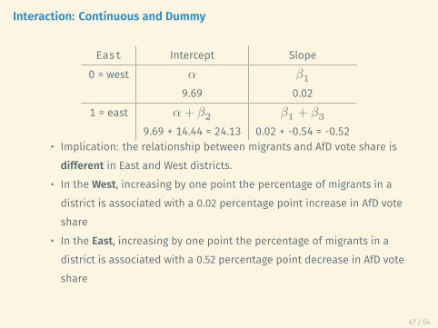
Interaction: Continuous and Dummy
East Intercept Slope0 = west 𝛼 𝛽1
9.69 0.021 = east 𝛼 + 𝛽2 𝛽1 + 𝛽3
9.69 + 14.44 = 24.13 0.02 + -0.54 = -0.52• Implication: the relationship between migrants and AfD vote share isdifferent in East and West districts.
• In the West, increasing by one point the percentage of migrants in adistrict is associated with a 0.02 percentage point increase in AfD voteshare
• In the East, increasing by one point the percentage of migrants in adistrict is associated with a 0.52 percentage point decrease in AfD voteshare
47 / 54

Interaction: Continuous and Dummy
East Intercept Slope0 = west 𝛼 𝛽1
9.69 0.021 = east 𝛼 + 𝛽2 𝛽1 + 𝛽3
9.69 + 14.44 = 24.13 0.02 + -0.54 = -0.52• 𝛽1
• The partial association between 𝑋1 and 𝑌 when 𝑋2 is equal to 0(holding other things constant)
• Here 𝛽1 describes the relationship between percentage of migrantsand the AfD’s vote share, for districts in West Germany
• 𝛽1 + 𝛽3• The partial association between 𝑋1 and 𝑌 when 𝑋2 is equal to 1(holding other things constant)
• Here 𝛽1 + 𝛽3 describes the relationship between percentage ofmigrants and the AfD’s vote share, for districts in East Germany
47 / 54

Interpreting the Constituents of the Interaction
Model 1(Intercept) 9.69
(0.66)migrantfraction 0.02
(0.03)east 14.44
(0.88)migrantfraction:east −0.54
(0.06)Adj. R2 0.66Num. obs. 299
• 𝛽1, the coefficient ofmigrantfraction, is theeffect of migration on voteshare when the dummy east is0, i.e. (in western districts)
• 𝛽2, the coefficient of east, isthe average difference betweenthe east and the west whenthere are 0% migrants
• 𝛽3, the coefficient of theinteraction, is the averagedifference in the effect ofmigrantfraction betweenthe east and west
48 / 54

Illustration
10 20 30 40
510
1520
2530
35
AfD vote share by migrant fraction
Share of migrants in district in %
AfD
vot
e sh
are
in %
• 𝛽2 the coefficient of east isnot the average differencebetween east and west
• 𝛽1 the coefficient ofmigrantfraction is not anunconditional effect ofmigration
• We do not have the general(unconditional) effects anymore
49 / 54
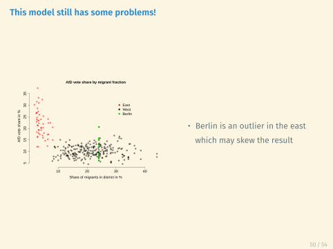
This model still has some problems!
10 20 30 40
510
1520
2530
35
AfD vote share by migrant fraction
Share of migrants in district in %
AfD
vot
e sh
are
in %
EastWestBerlin
• Berlin is an outlier in the eastwhich may skew the result
50 / 54

Multiple and Adjusted R^2

𝑅2 for the multiple regression model
𝑅2 is a useful general statistic:
• Simple linear regression
• 𝑅2 = proportion of the variance in 𝑌 explained by 𝑋
• Multiple linear regression
• 𝑅2 = proportion of the variance in 𝑌 explained by 𝑋1, ..., 𝑋𝑘
51 / 54
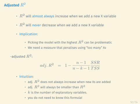
Adjusted𝑅2
• 𝑅2 will almost always increase when we add a new X variable
• 𝑅2 will never decrease when we add a new X variable
• Implication:
• Picking the model with the highest 𝑅2 can be problematic• We need a measure that penalises using “too many” Xs
-adjusted 𝑅2:
𝑎𝑑𝑗. 𝑅2 = 1 − 𝑛 − 1𝑛 − 𝑘 − 1
𝑆𝑆𝑅𝑇 𝑆𝑆
• Intuition:• adj. 𝑅2 does not always increase when new Xs are added• adj. 𝑅2 will always be smaller than 𝑅2
• 𝑘 is the number of explanatory variables.• you do not need to know this formula!
52 / 54

Conclusion
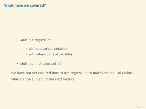
What have we covered?
• Multiple regression
• with categorical variables• with interactions of variables
• Multiple and adjusted 𝑅2
We have not yet covered how to use regression to make/test causal claims,which is the subject of the next lecture.
53 / 54

Seminar
In seminars this week, you will learn about …
1. Use of the lm() command to fit multiple linear regression models inR.
2. Use of the screenreg() command to compare differently specifiedmultiple regression models.
3. Interpretation of categorical variables and interactions betweenvariables.
4. 𝑅2 and adjusted-𝑅2
There will be no homework assignment at the end of the seminarassignment, because you will have your midterm assessment.
54 / 54