European Economic Review 37 (1993) 97-l 14. North-Holland

Public and private sector wages in the Netherlands*

Joop Hartog and Hessel Oosterbeek

University of Amsterdam, Amsterdam, Netherlands

Received September 1990, final version received November 1991

There is much debate in the Netherlands about underpayment of public sector workers relative to private sector workers. In this paper we analyze the wage structures in both sectors, using an endogenous switching regression model. Unlike previous Dutch studies, we find that the earnings prospects of public sector workers are better in the public sector than in the private sector. For private sector workers we find the exact opposite; their earnings prospects are better in the private sector. Moreover the allocation over sectors points to comparative advantages.

1. Introduction

Recently there has been lot of discussion in the Netherlands about the wages of public sector workers relative to the wages of their private sector equivalents. Until 1982 these wages were linked: The index of growth of private sector wages was directly applied to public sector wages. In 1982, however, this so-called ‘linking’ was abandoned, and since then public sector wages have fallen behind. Several studies reveal that, particularly at higher job levels, public sector workers are underpaid in the Netherlands.

Using a 1982 sample, Schippers (1986) estimates with OLS separate wage equations for public sector and private sector workers. He concludes that the returns to the human capital variables, education and on-the-job training (experience and experience squared), are more favorable in the private sector than in the public sector. Using a 1979 sample Van Schaaijk (1982) calculates for a number of different age/gender/education-groups the ratio of average public and private sector wages. He finds that in all age and schooling classes women earn more in the public sector. Males, on the other hand earn more in the public sector at lower levels of education, and less at higher educational levels. A similar finding is reported in Van Schaaijk

Correspondence to: Professor Joop Hartog, University of Amsterdam, Section of Micro- economics, Roetersstraat 11, 1018 WB Amsterdam, Netherlands.

*We benefited from discussions with Gerrit de Wit and from comments by Herbert Glejser, Joop Schippers, Jules Theeuwes, Jacques van der Gaag, Marein van Schaaijk, Wim Vijverberg and an anonymous referee.

00142921/93/$06.00 #J 1993-Elsevier Science Publishers B.V. All rights reserved

(1986). Theeuwes et al. ( 1985) report that in the 1979 data (the same data as Van Schaaijk used) life time human wealth is higher in the private sector for university educated workers and higher in the public sector for higher vocational and secondary educated workers.

The most important drawback of the approaches of Schippers and Van Schaaijk is that they ignore that the sector in which someone is working depends on decisions made by rational economic agents and is therefore endogenous. Several studies indicate that neglect of selectivity effects is likely to give a false picture of the relative earnings position of public sector workers. Venti (1987) analyses public/private sector wages in the United States with a model that takes account of selection bias. His main findings are: (i) the predicted wage difference between the federal sector and the private sector for males is about 4”,,; (ii) reductions of public sector wages of 16”, for men and 42”,, for women, will not cause an excess demand for public sector workers. The overpayment of 4% contrasts with earlier findings

for the United States by Smith (1976), who didn’t correct for selection bias and reported overpayment of public sector workers of no less than I I”,,. Comparably, from his application of the model to a sample of lawyers. Goddeeris (1988) concludes that ‘contrary to the impression one gets from estimating an earnings function for lawyers without accounting for self- selection, the results provide no evidence that those who choose public- interest law are generally accepting large sacrifices in earnings by virtue of that choice’. The estimation of earnings functions without taking account of self-selection, refers to Weisbrod (1983), who used the same sample and concluded that public sector lawyers are underpaid. Finally, Van der Gaag and Vijverberg (1988) who applied the model to a developing country (Cote d’Ivoire), report that OLS esitmates of wage equations may be biased since individuals sort themselves into the sector which pays them highest. Given these outcomes of earlier research, there seems to be no doubt that a conclusion of underpayment of public sector workers based on an estimation technique that doesn’t take account of selection bias, is not very reliable.

The research reported in this paper deviates in several respects from the studies mentioned above. Firstly, for a selection based analysis, one would prefer to have information with respect to relevant background characteris- tics of the decision-makers. Van der Gaag and Vijverberg, Goddeeris and Venti are restricted in this respect, whereas the empirical analysis in this paper is based on a rather unique data set, which contains, among others, information about family background and intelligence. Secondly, whereas in Goddeeris’ paper only the intercepts of the sector specific wage equations are allowed to differ, we permit both intercept and slopes to differ. Thirdly, Van der Gaag and Vijverberg estimate the influence of the wage differential on sector choice by a separate probit equation, whereas in our analysis this effect is estimated simultaneously.

J. Hartog and H. Oosterheek, Public and private sector wages in the Netherlands 99

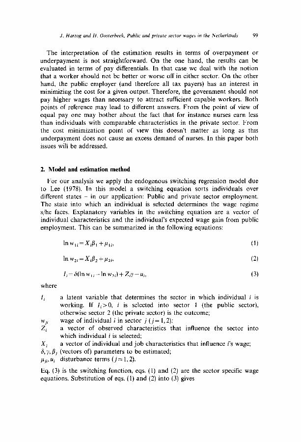
The interpretation of the estimation results in terms of overpayment or underpayment is not straightforward. On the one hand, the results can be evaluated in terms of pay differentials. In that case we deal with the notion that a worker should not be better or worse off in either sector. On the other hand, the public employer (and therefore all tax payers) has an interest in minimizing the cost for a given output. Therefore, the government should not pay higher wages than necessary to attract sufficient capable workers. Both points of reference may lead to different answers. From the point of view of equal pay one may bother about the fact that for instance nurses earn less than individuals with comparable characteristics in the private sector. From the cost minimization point of view this doesn’t matter as long as this underpayment does not cause an excess demand of nurses. In this paper both issues will be addressed.

2. Model and estimation method

For our analysis we apply the endogenous switching regression model due to Lee (1978). In this model a switching equation sorts individuals over different states - in our application: Public and private sector employment. The state into which an individual is selected determines the wage regime s/he faces. Explanatory variables in the switching equation are a vector of individual characteristics and the individual’s expected wage gain from public employment. This can be summarized in the following equations:

lnWli=XiPl +Pli,

ln w2i = xiP2 + PLzi,

Ii=6(lnw,i-lnw2i)+Zi~-~i, (3)

where

Ii a latent variable that determines the sector in which individual i is working. If Ii>O, i is selected into sector 1 (the public sector), otherwise sector 2 (the private sector) is the outcome;

wji wage of individual i in sector j (j= 1,2);

zi a vector of observed characteristics that influence the sector into which individual i is selected;

xi a vector of individual and job characteristics that influence i’s wage; 6,y,Bj (vectors of) parameters to be estimated; pji, ui disturbance terms ( j = 1,2).

Eq. (3) is the switching function, eqs. (1) and (2) are the sector specific wage equations. Substitution of eqs. (1) and (2) into (3) gives

100 J. Hartog and II. Oosterheek, Public and private sector wages in the Netherlunds

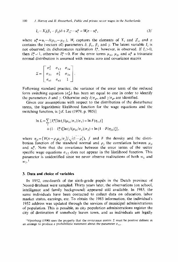
Ii=Xi(B1 -B2)6+Za_Ui* = CI/;~-UUT, (3)’

where u*=ui-6(~rj-,uZ,), K captures the elements of Xi and Zi, and rr contains the (vectors of) parameters 6, /Jr, pZ and y. The latent variable Ii is not observed; its dichotomous realization IT, however, is observed. If Ii>O, then 1: = 1, otherwise 1: =O. For the error terms pri, pZi and UT a trivariate

normal distribution is assumed with means zero and covariance matrix

2 01 012 01”

c= cr2, L I 0: ffzu

(T ul G”2 1

Following standard practice, the variance of the error term of the reduced form switching equation (a$) has been set equal to one in order to identify the parameters 6 and 1’. Otherwise only S/C,,*, and y/o”* are identified.

Given our assumptions with respect to the distribution of the disturbance terms, the logarithmic likelihood function for the wage equations and the switching function, is [cf. Lee (1979, p. 98.5)]

where ylji = [ cI/;n - /jjpji/aj]/J( 1 - pf), f’ and F the density and the distri- bution function of the standard normal and pi the correlation between pji and ~7, Note that the covariance between the error terms of the sector specific wage equations cr12 does not appear in the likelihood function. This parameter is unidentified since we never observe realizations of both u’r and W2.1

3. Data and choice of variables

In 1952, one-fourth of the sixth-grade pupils in the Dutch province of Noord-Brabant were sampled. Thirty years later, the observations (on school, intelligence and family background) appeared still available. In 1983, the same individuals have been contacted to collect data on education, labor market status, earnings, etc. To obtain the 1983 information, the individual’s 1952 address was updated through the services of municipal administrations of population. This is possible, as city population administrations register the city of destination if somebody leaves town, and as individuals are legally

‘Vijverberg (1990) uses the property that the covariance matrix Z must be positive detinite in an attempt to produce a probabilistic statement about the parameter CT, z.

J. Hartog and H. Oosterheek, Public and private sector wages in the Netherlands 101

compelled to register. A questionnaire was sent to all individuals for whom a valid address was found (some 4,700 out of 5,800 original observations). After mailing two reminders, the remaining male non-respondents were approached by an interviewer. It was decided (for budgetary reasons) to approach only men because of their higher labor force participation rate. The responses on the basis of the 4,700 addresses is 580/,.

The sample has some distinct features that are worth pointing out. It was already mentioned that all observations are originally from the same region, the province of Noord-Brabant. Earlier analysis [Hartog and Pfann (1985)12 indicated that this does not necessarily harm representativeness for the Netherlands, as many variables relating to labor force participation, industrial structure and earnings in Noord-Brabant do not differ much from values observed for the Netherlands. Also analysis of non-response in Hartog (1989) showed that the different sampling procedures for males and females, while affecting the level of non-response, did not affect structural relations; moreover, the selectivity term in separate wage equations for males and females was not significant. This suggests that selectivity problems due to non-response need not be a serious problem, although it must be admitted that non-response effects were not analyzed within the present model.

The dependent variables in the model are the sector in which someone is working (public or private sector), and the wage s/he earns. Therefore estimation of the likelihood function is restricted to the observations in the sample who work either in the public or in the private sector, where private sector only consists of individuals who work in paid employment (self- employed persons are excluded from the analysis). Since the wage determin- ation of employees in subsidized sectors is very similar to that for civil servants, the term public sector includes both civil servants and employees of the subsidized sectors. The data do not allow distinction between these sectors. The proportion of public sector workers in this sense in our sample (35.8’;/,) is about the same as in the labor force [cf. Centraal Bureau voor de Statistiek (1986, table 16)].

The wage is calculated by dividing reported after tax wage per period by reported number of hours worked during this period. Wages may not be homogeneous in hours. A study of the proper relation between hours and wage rate is a problem in itself, which we ignore here. As a simple approximation we include hours in the list of explanatory variables. Estim- ation is therefore further restricted to those observations for which after tax wage per hour could be calculated. Since net wages are used it is necessary to consider the fact that not all individuals face the same tax regime. Tax deductions for married women and nonmarried parents differ from those for married males. The consequence for net wages depends on the incidence of

*This report contains a detailed description, in Dutch, of the data set.

102 J. lfartog and H. Oosterheek, Public and private sector wages in the Netherlands

the income tax. If all workers fully shift the tax, their relative net wage is not affected by the tax regime, and can be ignored. If they fully bear the burden, their net wages fully reflect these burdens. Incomplete tax shifting is allowed for by including dummies for the relevant different treatment groups. The coefficient then is a measure of tax shifting, with zero effect indicating full shifting.

Identification in the endogenous switching regression model is of crucial importance. To identify the important parameter 6, at least one variable that enters wage equations (l)-(2) should not appear in switching function (3).3 But even if that condition is fulfilled, it should be noted that 6 is manipulable. Identifying on variables for which (pi -p2)y20 (where y is the coefficient that the left out variable would have had in the switching function) gives an upward (downward) bias to 6.

We have chosen to nearly separate the vectors Z and X, in order to avoid that identification of 6 depends on the choice of one or a few variables. Social background characteristics are supposed only to affect sector selection and not wages. On the other hand, tax-shift dummies, on-the-job training variables (experience, experience squared and years of general training) and job characteristics (hours worked and job level) are included in the wage equations and not in the switching function. It is likely that both wages and sector selection depend on education. In the analysis, actual years of education are included in the wage equations and level of education (effective education) in the switching function. This reflects that wages depend on what someone has learned (the human capital view), whereas in the selection process education is used as a filter by the employer or as a signal by the employee (the screening’ or signalling view) [cf. Groot and Oosterbeek (1990)]. The only variables that appear in both the wage equations and the switching function are IQ, gender and a dummy for non-graduation.

The labels of most of the variables are self-explanatory. A few of them, however, need some explanation. In the original questionnaire 15 categories for father’s occupation are distinguished. This information is compressed into four categories. Low-level occupations are lower clerical personnel, farm laborers, industrial laborers, other laborers and a few categories with a very small number of individuals (disabled, retired, temporarily not working). High level occupations are secondary school and university teachers and managers. Middle level occupations are made up of primary school teachers and intermediary employees. Self-employed fathers are a separate category.

‘In a recent paper Van Ophem (1992) proposes a modification of the switching regression model in which this identification restriction is not necessary. For the observed sector, he includes realized instead of expected earnings in the selection equation. The resulting likelihood function is rather complicated due to heteroscedasticity of the error term of the selection function. An unattractive feature of the model is that in fact, 6 is identifted on the residual of the wage equation; consequently, the better the wage equation, the poorer the identification of 6.

J. Hartog and H. Oosterheek, Public and private sector wages in the Netherlands 103

Table 1

Wage equations (absolute t-values in parentheses).

Regressor Public sector Private sector

Constant Years of education/l0 Experience/lo Experience sq/lOO Not married Female

Adjusted R2 F-value Number of observations

2.48 (8.66)” 0.28 (5.31) 0.44(1.72)

-0.13(2.29) -0.09 ( 1.44) -0.00(0.09)

0.22 19.9”

338

2.37 (16.8) 0.33 (9.06) 0.39 (2.93)

-0.1 l(3.59)” -0.04(1.22) -0.35(12.9)”

0.39 78.7”

605

“Significant at the 5%~level.

Unfortunately, it is not known whether the father worked in the public or in the private sector. The child’s ability was measured as an IQ test score. The test used in the empirical analysis was an already existing standard test that consisted of six subtests, relating to numbers, words, analogies and spatial orientation. The variable job level is measured on a seven point scale developed by the Dutch Department of Labor. The lowest level, level 1, covers very simple work where proficiency is attained in a few days of experience. The highest level, level 7, covers work on a scientific basis.

The appendix to this paper provides a description of all variables in terms of mean value and standard deviation for both sectors. This description is restricted to the cases that will be used in the empirical analysis.

4. Empirical results

Before turning to the estimation results of the model described in section 2, we first report the results obtained by re-estimating with the Brabant data the analyses of Schippers and Van Schaaijk as discussed in the introduction.

Table 1 contains the results of the estimation of the wage equations using the same explanatory variables as Schippers did; the only exception is that the variable age is missing in the Brabant data because everyone is about the same age. The earnings concept in these regressions is hourly wage. Based on the point estimates it turns out that with respect to the variable education the same conclusion is reached as Schippers’, namely that the returns to education are higher in the private than in the public sector.4 With respect to the variables experience and experience squared, which are supposed to measure the effect of on-the-job training, the finding is ambiguous. Up to 36 years of experience, the wage+xperience profile for someone with no

4At common levels of significance (5 or 10%) equality of the coefficients cannot be rejected. But since Schippers does not test the significance of the difference, we base our comparison on the point estimates.

104 J. Hartog and H. Oosterbeek, Public and priuate sector wages in the Netherlands

additional education, in the public sector exceeds that in the private sector. After 36 years the picture reverses. For someone with five years of additional education the take over year is 34. Schippers on the other hand calculates that with one exception the private wageexperience profiles lie always above the public sector profiles. This deviation might be due to the specific feature of the Brabant sample that all individuals are about the same age and therefore almost all of them fall within a narrow experience interval. Obviously, the sample is ill-suited for an analysis of the effect of experience on earnings and earnings differentials between sectors. The smaller wage gap for females in the public sector is similar to Schipper’s result.

Calculation of the ratio of average wages of public and private sector workers for six gender/education groups gives results that are pretty close to those reported by Van Schaaijk. We conclude therefore that it is possible to replicate earlier findings with the Brabant data. This implies that deviations of the empirical results of the analysis in this paper and the former analyses are due to the fact that a richer data set and a superior estimation method will be used, and not to any special feature of the sample.

The estimation results of the switching model are presented in table 2. The first two columns contain the results for the wage equations, the third column shows the estimates for the switching equation.

With respect to the results of the wage equations the following remarks can be made. In both the public and the private sector the hourly wage rate increases with: More years of education, a higher IQ, a lower number of working hours, and a higher job level. These results are mostly well known and repeatedly found. The depressing effect of more hours on the hourly wage rate is found in other Dutch studies as well; it may be a tax effect or be due to an upward bias in reported hours. Moffitt (1984) finds a U-shaped effect of hours on hourly wages. Comparing the coefficients of the variables in both sectors, it turns out that the effects of years of general training, years of education, job level, being female and working less hours are more favorable in the public than in the private sector. This result with respect to the effect of the job level contradicts Van Schaaijk’s finding that under- payment in the public sector increases with job level5 With respect to the other variables:

-As before, the coefficients of experience and experience squared show the well-known parabolic experience-wage profile;

-In both sectors non-graduation has a negative impact on wages, but in neither sector is this effect significant;

-Non-married parents have no different wages than males: Their different tax treatment is annihilated. Married females have an equally disadvan-

SUnfortunately the number of ‘high job level’-individuals in the sample is too small to carry out the analysis separately for this group.

.I. Hartog and H. Oosterbeek, Public and private sector wages in the Netherlands

Table 2

105

Public and private sector wage equations and sector selection function.a.b

Wage equations

Public sector Private sector Selection function

Constant

Social background Number of siblings/l00 Father’s occupation:

High Intermediate Independent

Education father Education mother

Personal characteristics

IQ/loo Extended primary = 1 Intermediate= I Higher vocational = 1 University= 1 Not graduated = 1 Years of education Years of general training Female = 1 Other variables Hours worked Job level Experience Experience squared/100

Tax dummies Married female = I Nonmarried parent = I Wage differential (6)

01 02 PI P2

Number of observations log L log L baseline Likelihood ratio ( - 21)

2.341(9.02)* 2.310(14.7)*

_ _ 0.356(0.26)

0.232( 1.80)** 0.214(2.70)* _ _ _ _ _ _

-0.047 ( 1.08)

_

- 0.035 ( 1.42) 0.030 (5.62)* 0.017(4.10)* 0.082 (4.63)* 0.021(1.61)

- 0.064 (0.83) -0.355(6.18)*

-0.023(11.2)* -0.007(3.85)* 0.078(6.43)* 0.058 (8.36)* 0.047 (2.24)* 0.025 (2.23)*

-0.126(2.61)* -0.075(2.83)*

-0.367(3.95)* - 0.073 ( 1.09) -0.112(0.95) 0.388 (0.61)

;.336( 16.5)*

_ _

0.230(21.6)* -0.842(22.5)* _

_ 0.251 (0.91)

338 605 -515.60 -932.51

833.82*

0.449 ( 1.03)

-0.013(0.06) -0.017(0.11)

0.085 ( 1.00) 0.114(1.81)**

-0.085(1.05)

-0.598( 1.76)** -0.028 (0.22)

0.147(0.95) 0.601(3.31)* 0.614(2.51)*

-0.168(1.51) _

-0.463 (2.99)*

_ _ _ _

_

;.222(5.57)* _

_ _

943

“Absolute value of asymptotic t-values in brackets. b*Significant at the 5%-level; **Significant at the IO%-level.

taged position in both sectors relative to males (the sum of the female and married female dummy coeffkients is -0.43 in both sectors). Unmarried females are worse off in the private sector, but not in the public sector.

Of some special interest are the signs of the correlation coefficients p1 and p2. These correlations appear in the conditional expectations of the wages:

106 J. Hartog and II. Oostrrheek. Public, und primte .wctor wges in the Netherlatuls

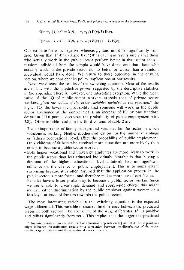
E(ln U’2i 1 1; < 0) = XJ2 + a,pJ’( l4$~)/( 1 ~ F( WX)).

Our estimate for p1 is negative, whereas p2 does not differ significantly from zero. Given that ,f‘( I&Z) > 0 and 0 < F( B$rr) < 1, these results imply that those who actually work in the public sector perform better in that sector than a random individual from the sample would have done, and that those who actually work in the private sector do no better or worse than a random individual would have done. We return to these outcomes in the ensuing section, where we consider the policy implications of our results.

Next, we discuss the results of the switching equation. Most of the results are in line with the ‘predictive power’ suggested by the descriptive statistics in the appendix. There is, however, one interesting exception. While the mean value of the IQ of public sector workers exceeds that of private sector workers, given the calues of‘ the other vuriahies included in the equation,’ the higher IQ, the lower the probability that someone will work in the public sector. Evaluated at the sample means, an increase of IQ by one standard deviation (13.6 points) decreases the probability of public employment with 3.8’?,,. Other notable results in the third column of table 2 are:

-The unimportance of family background variables for the sector in which someone is working. Neither mother’s education nor the number of siblings or father’s occupational level, affect the probability of public employment. Only children of fathers who received more education are more likely than others to become a public sector worker.

-Both higher vocational and university graduates are more likely to work in the public sector than less educated individuals. Notable is that having a diploma of the highest educational level attained, has no significant influence on the chance of public emplopyment. This is to some extent surprising because it is often assumed that the application process in the public sector is more formal and therefore makes more use of certificates.

~ Females have a lower probability to become a public sector worker. Since we are unable to disentangle demand and supply-side effects, this might indicate either discrimination by the public employer against women or a less loyal attitude of females towards the public sector.

The most interesting variable in the switching equation is the expected wage differential. This variable measures the difference between the predicted wages in both sectors. The coefficient of the wage differential (6) is positive and differs significantly from zero. This implies that the larger the predicted

“This interpretation ignores that level of education depends on IQ and that this dependency might influence the estimation results by a correlation between the disturbances of the sector specific wage equations and the educational choice function.

J. Hartog and H. Oosterheek, Public and private sector wages in the Netherlands 107

wage gain from working in the public instead of the private sector, the more likely it is that an individual is selected into the public sector. This variable will be discussed in more detail below.

5. Policy implications

In the introduction it was mentioned that for the comparison of public and private sector wages at least two points of reference are relevant. Equity considerations will stress equal pay for equal workers, whereas efficiency aspects underscore that an employer (the government) should not pay higher wages than necessary to attract enough capable workers. This section first deals with pay differentials and then treats the cost minimization aspect.

The classical approach to the question whether discrimination is at stake, makes use of OLS estimates of wage equations. This approach is adopted by researchers in the fields of race and sex discrimination. It is applied to the case of public-private wage comparisons by, among others, Smith (1976) and Weisbrod (1983). From the discussion of the endogenous switching regression model in section 2 it is clear that this approach ignores the fact that (unlike sex and race) public employment is a choice variable. It is, however, interesting to compare the results of the naive approach with the approach adopted here.

Smith (1976) decomposes the percentage of pay differential into a portion attributable to observed characteristics and a portion that remains and is determined by differences between the coefticients in the wage equations in both sectors. The second portion is referred to as discrimination. An important question is what the wage structure would have been in the absence of discrimination. Since this question is unanswerable, one has to choose either the public sector or the private sector structure as basis of reference. In our analysis we will use both bases. In her decomposition Smith calculates what a worker who works in the public sector would have earned in the private sector, given the wage structure in that sector and his characteristics. This imputed alternative wage is compared with his actual wage in the public sector. This seems incorrect, since actual wage includes a random component, whereas the calculated alternative doesn’t. We will therefore compare expected wages in both states.

First, expected wages are calculated using OLS estimates of the sector specific wage equations.’ Second, the same calculations were performed using the estimates of the endogenous switching regression (ESR) model. In

‘These wage equations have the same specification as those in table 2.

108 J. Hut-tog and H. Oosterheek. Public and private sector wages in the Netherland.~

Table 3

Predicted average public and private sector wage rates (guilders).

Lower educuted

Public sector workers (21 I cases) In public sector In private sector

Private sector workers (529 cases) In public sector In private sector

Higher edwutrd

Public sector workers (127 cases) In public sector In private sector

Private sector workers (76 cases) In public sector In private sector

OLS ESR

16.07 16.37 14.45 13.1 I

15.28 9.71 13.97 13.98

21.66 21.33 18.90 17.26

19.27 12.1’) 18.95 I X.96

the literature there is some disagreement whether to use the conditional or the unconditional expectations to evaluate the results. Bjorklund (1983) defines the unconditional effects as the effects on the prospects facing the whole population before the choice is made, and the conditional effects as the effects for those who actually have made the choice to become a public or private sector worker. The latter concept seems most appropriate to evaluate the earnings position of those who presently work in the public (private) sector [see also Maddala (1983, p. 260), Van der Gaag and Vijverberg (1988, p. 250) and Bjorklund and Moffitt (1987, p. 44)]: It includes the sector-specific expected earnings effect of unobserved characteristics. For the conditional expectations one ought to compare

with

for those who work in the public sector, and

E(ln rvzi / Ii ~0) = Xi/l1 ~ rr,p,,/‘( Wn)/( 1 - F( Wrr))

with

for the private sector workers. In table 3 we present the conditional predictions. The wages are calculated separately for lower and higher educated workers.

J. Hartog and H. Oosterbeek, Public and private sector wages in the Netherlands 109

The results in the second column of table 3 indicate that the earnings prospects for both higher and lower educated public sector workers are more favorable in the public sector than in the private sector. Higher educated public sector workers gain 23.6% (21.33 versus 17.26) from public employ- ment, and lower educated public servants gain 24.9% (16.37 versus 13.11). For private sector employees the exact opposite holds; their earnings prospects are better in the private sector than in the public sector. Their gain from working in the private sector equals 44% for lower educated (13.98 versus 9.71) and 55.5% for higher educated (18.96 versus 12.19). We might therefore conclude that from the point of view of earnings maximization the present allocation of workers over sectors is efficient.

The results in the second column also reveal that public sector workers perform better in the public sector than private sector workers would have done (21.33 > 12.19 and 16.37 > 9.71). Similarly, private sector workers do better in the private sector than public sector workers would have done ( 18.96 > 17.26 and 13.98 > 13.11). The results point to a clear case of absolute (and thus comparative) advantage.

The differences between the results in the first (OLS) and second (ESR) columns in table 3 also stress the importance of correction for selectivity bias. The main differences are that: (i) the earnings differentials for public sector workers calculated from the OLS estimates are much smaller than the ESR results; (ii) according to the OLS results private sector workers have better prospects in the public sector than in the private sector; and (iii) for lower educated workers absolute advantage no longer holds; only the weaker condition of comparative advantage is fulfilled (16.07/14.45 > 15.28/13.97).

An interesting reinterpretation of the switching regression model has been proposed by Bjiirklund and Mofitt (1987). In the model in section 2 we have set cu* equal to one in order to identify 6 and y. Bjijrklund and Moffltt argue that economic theory restricts 6 to be equal to one - the decision must be a direct function of the wage gain (p. 45, fn. 4). By this restriction it is possible to identify G”*. Furthermore (minus) Zy is interpreted as the costs of joining the public sector. As a result of this reinterpretation it is now possible to calculate the expected values of the net value (the welfare gain) of working in the public sector: E(li 11: = 1) = Xi(pI - flz) + Ziy + u&, with Ai = -f( I++c)/F( PI+) for public sector workers. For private sector workers ibi = f( IQc)/( 1 - F( CI/IX)).~ Using this expression we find that for public sector workers the average welfare gain of working in the public sector is 32.4% of the wage. For private sector workers the welfare gain from public(!) employment would on average be 3.2% of the wage. For both groups the welfare gain from public employment exceeds the wage gain from public

sThe estimate for 7 in the Bjiirklund and Moffltt model equals l/6 times the estimate for 1 from the likelihood function given in section 2: The eNects of Z-variables are measured in monetary equivalents.

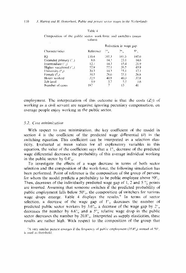
Table 4

Composition of the public sector work-force and switchers (mean \alues).

Characteristics

IQ Extended primary (‘I,,) Intermediate (“,,) Higher vocational I”,,) Universitv (” ) Female (“,,I ‘I Hours worked Job level Number of cases

Reduction in wage gap

Reference I”,, 2”,, 5”,,

I IO.4 107.3 107.5 107.0 X.6 14.3 33.1 14.6

12.7 14.3 I s.4 2 I .Y 57.‘) 51. I 3x.5 43.‘) 203 142 73.1 17. I 34.5 2X.6 23. I 16.8 32.0 40.‘) 40.3 37.8

5.‘) 5.7 5.5 5.6 lY7 7 I3 41

employment. The interpretation of this outcome is that the costs (Zy) of working as a civil servant are negative; ignoring pecuniary compensation. on average people enjoy working in the public sector.

5.2. Cost minimixitioti

With respect to cost minimization, the key coefficient of the model in section 4 is the coefficient of the predicted wage differential (6) in the switching equation. This coefficient can be interpreted as a selection elas- ticity. Evaluated at mean values for all explanatory variables in this equation, the value of the coefficient says that a l”,, decrease of the predicted wage differential decreases the probability of this average individual working in the public sector by 0.4”,,.

To investigate the effects of a wage decrease in terms of both sector selection and the composition of the work-force, the following simulation has been performed. Point of reference is the composition of the group of persons for whom the model predicts a probability to be public employee above 9.X,,. Then, decreases of the individually predicted wage gap of 1, 2 and 5 “; points are inserted. Assuming that someone switches if the predicted probability of public employment falls below 50?,, the composition of switchers for various wage drops emerge. Table 4 displays the results.” In terms of sector selection. a decrease of the wage gap of I”,, decreases the number of predicted public sector workers by 3.6”,, a decrease of the wage gap by 2”,, decreases the number by 6.6:‘” and a S’,, relative wage drop in the public sector decreases the number by 20.X”,,. Interpreted as supply elasticities, these results are rather high. With respect to the composition of the group that

‘A very similar picture emerges if the l”requencq of public employment (35.X”,,) instead of 50”,, is used a\ threshold.

J. Hartog and H. Oosterbeek, Public and private sector wages in the Netherlands 111

leaves the public sector, one would expect the most deviant composition for the early leaves, and a convergence to the average characteristics when more people switch. This is only the case for composition by working hours. It does not hold for IQ, job level, education and gender. Looking at the composition of the 41 workers predicted to leave after a So/, wage drop, it appears that mainly low educated males, who work long hours, are inclined to leave the public sector. This prediction is in contrast to anecdotal evidence and newspaper stories about top level civil servants switching to the private sector. Apparently this creates a false picture.”

6. Conclusions

In this paper the factors that determine the sector of employment and the wage structures in the public and private sector have been investigated.

Clear support is found for the endogenous switching model. An indivi- dual’s predicted wage differential between sectors has a significant effect on the individual’s sector of work. OLS estimation of wage equations gives biased estimates, in particular for workers in the private sector. The probability of public sector employment correlates negatively with IQ, and positively with human capital variables as higher vocational and university education.

The model is used to investigate whether public sector workers are underpaid relative to private sector workers. Earlier research (and public debate) concluded indeed to underpayment. However, this research at best used wage equations estimated with OLS. Common results are that the government pays less for education and on-the-job training, and hence, that especially higher level civil servants are underpaid. In contrast, the results reported in this paper indicate that both higher and lower educated public servants would experience a large wage loss if they switch sectors. On the other hand, however, private sector workers would earn lower wages after a switch as well. Calculation of the welfare gains reveals that all workers would prolit from public employment, but the gain for those already working in the public sector is much larger than the gain for those presently working in the private sector (32.4 versus 3.2% of the wage). We might therefore conclude that the present allocation of workers over sectors is efficient both from an earnings and a welfare maximization point of view.

Comparison of the wages of public and private sector workers in both sectors also reveals that public sector workers earn more in the public sector than private sector workers would have done, and vice versa, that private sector workers perform better in the private sector than public sector

“Research with recent (1985%86,88) panel data corroborates this; with respect to level of education, Mekkelholt and Oosterbeek (1991) find that switchers from the public sector are lower educated than stayers.

workers would have done. Hence our results point to the presence of absolute (and therefore comparative) advantage.

As the results deviate from earlier research as well as from communis opinio, it is important to note that the data used in this paper would generate the same conclusions as others found if their methods are applied. It is also important to be aware of the fact that a special data set has been used: All individuals about 40 years old, all living in the province of Noord- Brabant in 1952. The latter fact might for example lead to an overrepresent- ation of workers in local and provincial government relative to central government, with a somewhat different pay structure. But since it was possible to reproduce others’ results, it seems unlikely that this causes serious errors. So, there is evidence to believe that our results point to real effects rather than peculiarities of the data set.

Finally, the model has been used to simulate effects of changes in the wage gap. The selection elasticity of the relative public wage is found to be around 4. It is also found that after a wage drop in the public sector. switchers are on average low educated males who work long hours. This is also contrary to the public opinion, although it should be stressed that the results apply to 1983. As the public sector average wage started to lag seriously after 1982, it would be worthwhile to repeat the analyses with more recent data.

J. Hartog and H. Oosterheek, Public and private sector wages in the Netherlands 113

AQQendix

Table A.1

Descriptive statistics: Mean values and standard deviations.

Variable

In hourly wage

Social background:

Number of siblings Father’s occupation:

High (2,) Intermediate (y,,) Low (I;:,) Self employed (%,)

Father’s education level (l-6) Mother’s education level (l-6)

Individual’s qualities:

IQ Education:

Primary (“l;,) Extended primary (‘:b) Intermediate (y;,) Higher vocational (“4,) University (‘:A) Not graduated &,) Years of education

General training (in years)

Other variables

Female (“b) Married female (I>,,) NonmarrIed parent (“/A) Hours worked Job level (scale l-7) Experience (years)

Number of cases

References

Public sector

1.890

-Private sector

2.68 (0.32)

4.89(2.73) 4.79(2.55)

5.0 3.5 15.4 11.4 50.6 60.3 29.0 24.8

2.54 (0.90) 2.35 (0.62) 2.32 (0.67) 2.21(0.49)

lO5.2( 14.3) 102.8(13.1)

10.3 15.8 35.2 56.0 16.9 15.7 28.1 9.9

9.5 2.6 IS.1 20.5 11.99(4.36) 10.03(3.27) 0.56 (0.96) 0.44 (0.69)

23.7 18.3

I.8 37.2( 11.6)

4.9 ( I .70) 24.5(4.50)

338

17.3 14.7 2.1

39.3 (10.6) 4.3 ( 1.69)

26.0(4.13)

605

Bjiirklund, Anders, 1983, A note on the interpretation of Lee’s self-selection model, Mimeo. (Industrial Institute for Economic and Social Research, Stockholm).

Bjiirklund, Anders and Robert Moflitt, 1987, The estimation of wage gains and welfare gains in self-selection models, The Review of Economics and Statistics 69, 42-49.

Centraal Bureau voor de Statistiek, 1986, Arbeidskrachtentelling 1983 (Staatsuitgeverij, The Hague).

Goddeeris, John H., 1988, Compensating differentials and self-selection: An application to lawyers, Journal of Political Economy 96, 41 l-428.

Groot, Wim and Hessel Oosterbeek, 1990, Does it pay to take the shortest way?; Incidence and labor market consequences of class repetitions, dropping out and inellicient routing in education, UvA/FEE Research Memorandum 9013 (University of Amsterdam, Amsterdam).

Hartog, Joop, 1989, Survey non-response in relation to ability and family background: Structure and effects on estimated earnings functions, Applied Economics 21, 387-395.

Hartog, Joop and Gerard Pfann, 1985, Vervolgonderzoek Noordbrabantse zesdeklassers (University of Amsterdam, Amsterdam).

Lee. Lung-Fe]. 1978. Unionism and wage rates: A simultaneous equations model with quahtative and limited dependent variables. International Economic Review 19, 41-433.

Lee. Lung-Fel, lY79. Identification and estimatmn 1n binary choice models with llmited (censored) dependent variables. Econometrica 47, Y77 998.

Maddala. Gary. lY83. Limited-dependent and qualitative variables in econometrics (Cambridge l!niverbity Press, Cambridge).

Mekkelholt Eddie W. and Hessel Oosterbeek. IYYI, Overheldsector en marktsector: loon\er- schillen en mohiliteit. in: Eddie Mekkelholt. Erik Brouwer and William Pratt. eds,

Arbeidsmohiliteit en belonlng in Nederland. OSA-werhdocument WXX (Organisatie \oor Strategisch Arheidsmarktonderroek. The Hague).

Moffitt. Robert. 1984, The estimation of :L joint wage-hours labor supply model. Journal of Labor Economics 7. 550 566.

Roy. A.D.. lY5l. Some thoughts on the distrlbutlon of earning\. C>xford Economic Papers .3. 135 146.

Schippers. Joop. 1986. Memelijh hapltaal en heloninga~crschlllen, Economisch Statwtlwhe Berichten, 576 5X0.

Smith, Sharon. 1976. Pa) dlfferentials between federal government and private hector worhe1.s. Industrial and Labor Rclatlons Review ?Y, I79 107.

Theeuues. Jules, Carl Koopmans, Rocus \an Opstal and H. van Re?)n. 19x5, Estimation ol human capital accumulation parameters for the Netherlands. European Fconomlc Rebleu 2Y. 233 757.

Van der Haag. Jacques and Wim Vijverberg. IYXX. A buitching regression model for v,age determinants in the public and private sectors of a developing country. The Revieu 01 Economics and Statistics 70. 244 252.

Van Ophem, Hans. 1992. .A modified suitching regrewon model for earnings differentials between public and private sectors in the Netherlands. The Review of Economics and Statistics. forthcoming.

Van Schaaijk. Marein, 19x7. Een minipakketvergelijking. Economisch Statlstlsche Berichten. 1334 1337.

Van Schnaijk, Marein, lYX6. I’akketvergelijking, Economisch Statistische Berichten. 43X-440. Vent!. Steven. 19X7. Wages in the federal and prlvute sectors, in: D.A. Wise. ed. Public sector

payrolls (National Bureau of Economic Research. Cambridge. MA). ViJverherg. Wim P.M.. 1990. Identifying the unidentified parameter of the Roy model of

selectivity. Mimco. (School of Social Sciences University of Texas at Dallas, Dallas. TX). Wcishrod, Burton. 1983. Nonprofit and proprietary sector behavior: Wage differentials among

lan yew Journal of Labor Economics I. 246 263.