public disclosure authorized water quality...
TRANSCRIPT

Water QualityMod)eling
Mervin D. Palmer
22238May 2001
F
T HE WOR LD0 B AN K
Pub
lic D
iscl
osur
e A
utho
rized
Pub
lic D
iscl
osur
e A
utho
rized
Pub
lic D
iscl
osur
e A
utho
rized
Pub
lic D
iscl
osur
e A
utho
rized
Pub
lic D
iscl
osur
e A
utho
rized
Pub
lic D
iscl
osur
e A
utho
rized
Pub
lic D
iscl
osur
e A
utho
rized
Pub
lic D
iscl
osur
e A
utho
rized

Iola 4u°*%"AA,Stu% PIJOMA t1a1
3A3IIOVUd 314A13'JAA¶ 01 3ACIflD V
J;ug (I UHLluW
0 ,l ,1nii i ||| fiw~~~i allloj Igli11 I1
xI#lvn a?7 4

Copyright C) 2001 The International Bank for Reconstruction
and Development / THE WORLD BANK
1818 H Street, N.W.
W'ashington, D.C. 20433, USA
All rights reserved
Manufactured in the United States of America
First printing Miay 2001
1 2 3 4 05 04 03 02 01
The findings, interpretations, and conclusions expressed in this book are entirely those of the authors
and should not be attributed in any manner to the World Bank, to its affiliated organizations, or to
members of its Board of Executive Directors or the countries they represent. The World Bank does
not guarantee the accuracy of the data included in this publication and accepts no responsibility for
any consequence of their use. The boundaries, colors, denominations, and other information shown on
any map in this volume do not imply on the part of the World Bank Group any judgment on the legal
status of any territory or the endorsement or acceptance of such boundaries.
The material in this publication is copyrighted. The World Bank encourages dissemination of its
work and will normally grant permission to reproduce portions of the work promptly.
Permission to phstocoply items for internal or personal use, for the internal or personal use of spe-
cific clients, or for educational classroom use is granted by the WNorld Bank, provided that the appro-
priate fee is paid directly to the Copyright Clearance Center, Inc., 222 Rosewood Drive, Danvers, .NA
01923, USA; telephone 978-750-8400, fax 978-750-4470. Please contact the Copyright Clearance Cen-
ter before photocopying items.
For permission to reprinit individual articles or chapters, please fax a request with complete infor-
mation to the Republication Department, Copyright Clearance Center, fax 978-750-4470.
All other queries on rights and licenses should be addressed to the Office of the Publisher, World
Bank, at the address above or faxed to 202-522-2422.
Cover design by Tomoko Hirata
Library of Congresd Cataloging-in-Publication Data
Palmer, Mervin D., 1937-
NVater quality modeling: a guide to effective practice / by Mervin
D. Palmer.
p. cm.
Includes bibliographical references.
ISBN 0-8213-4863-9
1. Water Quality-Mathematical models. 2. WVater quality
management-Mathematical models. 3. Water quality-East
Asia-Mnviathematical models -Case studies. 1. Title.
TD370 P35 2001
363.739'42'015118-dc2l 00-049951
Contents
Acknowledgments .... vi
Foreword .................................... ix
Executive Summary .............................. xi
Chapter 1General Overview of Water Quality Modeling .... ..... 1
Modeling Costs ....................................... 4General Water Quality Model Components ...... ........... 5Typical Water Quality Model Applications ...... ............ 7
Chapter 2Water Quality Model Structure and Process ..... ..... t 1
Basic Definitions ..................................... 11Required Resources . .................................. 15Water Ouality Parameters ............. ................. 17Receiving Water Processes ....... ..................... 28
Chapter 3Some Commonly Used Models .................... 37
Hydrodynamic Model .................. ............... 37Mass Balance ........................................ 40Receiving Water Processes ............ ................. 43Selected Models ...................................... 51Model Data Requirements and Prediction Issues ..... ....... 59Quality Assurance and Quality Control ....... ............ 63
iii
C WATER QUALITY MODELING
Chapter 4Case Studies of Models Applied toWorld Bank Projects ........ ..................... 71
Detailed Hydrodynamic and Water Ouality Modeling Study,1998, Chongqing, China ......... ..................... 71Oceanographic and Water Quality Modeling Studies at Mumbai,India, 1997 .......................................... 80Hangzhou Bay Environmental Study, 1993-1996 ..... ....... 85Second Shanghai Sewerage Project (SSPII), 1996 .... ..... 90Shanghai Environment Project, 1994 ...... ............... 95Manila Second Sewage Project, 1996 ..................... 98Tarim Basin 11 Planning Project, 1997, China ..... ......... 102
Appendix .................................... 109
CE-OUAL-W2:A Numerical Two-Dimensional Laterally Averaged Model ofHydrodynamics and Water Quality ...... ................ 109CORMIX ......................................... 111DIVASTBinnie & Partners ............ ....................... 115HYDROLOGICAL SIMULATION PROGRAMI-FORTRAN(HSPF)User's Manual for Release 8.0 ....... ................... 117MIKE SYSTE M ............. ....................... 123QUAL2E & OUAL2E-UNCAS(6 April 1999) . ...................................... 131STORM WATER MANAGEMENT MODEL (SWMM)Version 4 Part A: User's Manual ....... ................. 137TRISULA - DELWAODelft Hydraulics ............. ....................... 142WQRRSWater Quality for River-Reservoir Systems ..... .......... 146
Glossary . .................................... 149
References ................................... 153
CONTENTS a
Tables
Table 2.1 Water Ouality Parameters Discussed inThis Manual ...................................... 18Table 3.1 Properties of Some Models ....... .............. 53
Figures
Figure 2.1 Dissolved Oxygen Process ..................... 20Figure 2.2 Nitrogen Processes ........................... 21Figure 2.3 Phosphorus Processes ......... ............... 22Figure 4.1 Simulated Concentrations Along Jialing River 1987. 74Figure 4.2 Schematic of Source Loadinga .................. 75Figure 4.3 Scenario 2 with Treatment Plants ...... ......... 76Figure 4.4 Scenario 3 with Interceptor Along Jialing River.... 77Figure 4.5 Simulated Maximum Concentrations of Ammonia inJanuary 1987 ...................................... 79Figure 4.6 Current Meter and Tide Gauge Locations andModel Area ....................................... 82Figure 4.7 Calibration Curve for Velocity and DirectionSpring Tidal Condition ................................. 83Figure 4.8 Fecal Coliform Densities at 3 and 8 kilometers forPrimary Treatment .................................... 84Figure 4.9 Hourly Variation in Fecal Coliforms Near 3 kmWorli Outfall .................................... 85Figure 4.10 Nested Finite Element Grid ....... ............ 87Figure 4.11 Hangzhou Bay Simulated Flow Field ..... ...... 88Figure 4.12 Hangzhou Bay Simulated Freshwater Fractionand Salinity Calibration ................................ 89Figure 4.13 The Model Domain ......... ................ 92Figure 4.14 Simulated Near-field Surface ConcentrationDistribution of Copper ................................. 94Figure 4.15 Simulated Current Velocity Vectors ............ 100Figure 4.16 Simulated Benthic Loadings .................. 101Figure 4.17 Tarim River Basin: Stage II Project Location .... 104Figure 4.18 Tarim II Preparatory Study: Study Activities .... 105Figure 4.19 Simulation of Bostan Lake ...... ............. 106

R WATER ~QUALIT~YMOD~ELING---
Figure CRX 1 Flow Classification System ..... ........... 113Figure CRX 2 Predictions versus Measurements ........... 114Figure HSP I Flow Diagram ....... ................... 119Figure HSP 2 Flow Diagram for Nitrogen Reactions ........ 120Figure HSP 3 Flow Diagram for Phosphorus Reactions ..... 121Figure HSP 4 Flow Diagram for Solids ..... ............. 122Figure MIK I Dissolved Oxygen Processes ..... .......... 129Figure iMIK 2 Nitrogen Processes ...... ................. 130Figure OUA 1 Stream Network of Computational Elementsand Reaches ........................................ 135Figure QUA 2 Discretized Stream System ..... ........... 136Figure SWM 1 Relationship Among SWWM Blocks ........ 139Figure SWM 2 Northwood (Baltimore) Drainage Basin"Coarse" Plan ....................... 140Figure SWM 3 Special Hydraulic Cases in EXTRAN Flow C 141Figure TRI I General Structure of the Modeling Framework . 144Figure TRI 2 Model Processes ...... ................... 145
Acknowledgments
P reparation of this guide was financed by the East Asia Socialand Environment Sector Unit (EASES) under the directionof Zafer Ecevit. The guide is the product of an extensive
review carried out by Merv Palmer under the guidance of GlennMorgan and Jack Fritz. The report has benefited greatly from thecontributions of others with diverse perspectives on water qualityprediction and management. In addition, the preparation of thereport has drawn extensively on the experience of institutions world-wide active in the development of water quality prediction models.
EASES gratefully acknowledges the significant advice providedby the following individuals: Geoffrey Read, Edouard Motte, andWiebe Moes of the East Asia Urban Development Unit. Doug Olsonof the East Asia Rural Development and Natural Resources Unitprovided technical inputs on case studies and contributed many hoursof peer review. Heinz Unger, Rob Crooks, Anil Somani, andPatchamathu Illangovan from EASES provided valuable insightsduring the conceptualization of the report. Editorial assistance indesign, layout, and preparation of illustrations was provided byMellen Candage, Catherine Fadel, Kaye Henry, and Nicola Marrian.
vii

Forew'ord
T he quality of surface water resources affects virtually allaspects of life in East Asia. Pollution from industrial, agricul-tural, and domestic sources continues to grow throughout the
region, affecting rivers, lakes, estuaries, and coastal regions. As pop-ulation growth with its attendant economic growth continuesthroughout the region, water resource managers must increasinglyuse analytical tools to assist in the formulation of sustainable watermanagement strategies. One family of analytical tools that can be oftremendous value are water quality prediction models.
Experience demonstrates that the design, implementation, andmonitoring of waste management schemes can benefit from the useof numerical modeling. The evolution of these prediction tools nowcreates many more opportunities for operational and economic opti-mization than were available a generation ago. Computer systemsand software are less expensive, more accessible, and easier to usethan ever before. At the same time, increased accessibility createsmore opportunity for misapplication under field conditions. To bemost effective, water quality prediction models must be used in waysappropriate to the task at hand; they require the expertise of knowl-edgeable technical specialists and reliable input data. Water qualityprediction can be expensive and potentially inconclusive if notapproached in a systematic manner.
This technical guide provides a review of the state of water qual-ity prediction models available to the practitioner today. It providesessential technical background for individuals who may be requiredto develop models or interpret their results in the context of projectdesign. The guide, which is designed as a more in-depth and revisedtreatment of this issue as presented in the World Bank's Pollution Pre-('ention anod Abatement Handbook 1998, will fill a significant gap in the
ix

E WATER QUALITY MODELING
technical literature. More important, it demonstrates how thesemodels have been applied to recent World Bank projects.
It is hoped that this publication will provide a technical discus-sion of water quality prediction that is accessible to practitioners indeveloping countries. We believe this will become an essential guidefor anyone involved in the design or use of water quality predictionmodels. In this way, the guide will contribute to the more effectiveuse of prediction tools and will improve the quality of water projectsin general.
Za/#er E&evitSector DirectorEnvironment and Social Development UnitEast Asia and Pacific RegionThe World Bank
Executive Summary
T he challenge of understanding and managing surface waterquality problems in East Asia is growing. Those responsiblefor managing water resources must look to a variety of ana-
lytical tools to design, implement, and monitor sustainable waterquality management programs. An important family of tools arenumerical water quality prediction models. With the availability ofpowerful desktop computers and the growing availability of soft-ware, these tools have become increasingly accessible.
Numerical models have demonstrated an impressive capacity tosupport important water resource decisions in developed countries.Models are typically used to support development and public policydecisions in a variety of areas: simulation of discharges, outfalls, andintakes; changes to wastewater treatment systems; approval ofchanges in industrial processes; operation of dams and reservoirs;and water resource allocations, among other uses. The value of mod-eling is important in economic and financial terms with regard todetermining particular project options and phased investment pro-grams.
Not all models, however, are appropriate under all conditions.They vary greatly with respect to their analytical approach, underly-ing assumptions, data needs, and output capacity. In the context ofdeveloping countries, the utility of models must be carefully exam-ined in the light of important constraints such as lack of experiencedtechnical staff, poor-quality data sets, and lack of or poorly enforcedquality control protocols.
This document serves as a guide to the utility and relevance ofwater quality prediction modeling. It draws upon examples fromrecent World Bank water resources and wastewater managementprojects. The goal of the guide is to provide a broad-based under-
xi
E WATER QUALITY MODELING
standing of the water quality prediction process and to evaluate therelative merits and cost-effectiveness of using water quality modelsunder field conditions. The guide builds on and revises the chapteron water quality modeling prepared for the World Bank's Pollutito
Pre(oen lion and Abatement Handbook, 1998.The guide does not address groundwater or air quality models.
The characteristics of such models are similar to those of water qual-ity models; consequently, understanding water quality models willmake it easier for users to become knowledgeable about groundwa-ter and air quality models. For more information on groundwatermodels, readers may refer to the World Bank publication, "Ground-water: Legal and Policy Perspectives"(technical Paper WTP 456,1999). For information on air pollution, readers may refer to theBank publication, Urban Air IQuality zAlanaqement Strateqy in A,4a:Guidebook 1997.
The guide is designed for a range of practitioners, including Banktask managers, environmental specialists, and counterpart technicalstaff involved in the design, evaluation, and monitoring of sustain-able water resources programs. It is not intended to be a compre-hensive review of all available water quality prediction models, norto be an endorsement of specific models. While some typical exam-ples of models are discussed in the report, it provides a thoroughreview of the current approaches to water quality modeling and thetypes of parameters that are typically modeled, and offers an assess-ment of the state of water quality modeling for each parameter.
To illustrate the myriad ways in which water quality predictionmodels have been used in practice, the guide presents a number ofcase studies from recent development project with World Bankfinancial support.. Each case study describes the manner in whichmodels have been used, the constraints encountered under field con-ditions, the results obtained, and the cost-effectiveness of each appli-cation. While the case studies are drawn from East Asian experience,they are relevant to and instructive for all regions.
-quite simple mathematical equations can model complex systems--sensitivity depends on initial conditions-
James Gleick, 1987 in "Chaos"

EXECUTIVE SUMMARY
The guide fills an important gap in the available literature on
water quality prediction models. It is designed to cover technical
material normally found in more exhaustive, but less accessible, text-
books. In addition, it attempts to bring together information on mod-
els that are currently available only through an assortment of
difficult-to-find technical references. Potential users of water quality
models will find in this guide the basics of commonly used models
and will learn how they can be effectively applied in a project con-
text. The guide addresses several inter-related questions:
* What types of models are available and how are they structured?
X AWhat are the basic parameters that models can predict, and how effec-
tively can these parameters be modeled?
* What specific models are available?
* Under what circumstances will water quality prediction models be
most beneficial?
* What are the cost and other practical implications of using models in a
project setting?
The guide comprises five sections. Chapter 1 provides a general
overview of the use of water quality models, including the objectivesof water quality modeling, the approach to water quality prediction,the costs of modeling processes, and the general components of typ-ical water quality models. Chapter 2 discusses the most commonwater quality parameters that are modeled, the receiving waterprocesses, quality assurance and control for the water quality dataand model predictions, and the required model resources. Chapter 3describes generic components of water quality models. In thisdescription, equations are presented. It is not necessary that thereader understand these equations fully, or their method of solution,but it is important to understand the complexity of the model pre-dictions and the requirements for site-specific data. Some predictionmodels are then discussed, with detailed summaries of these modelspresented in an Appendix.
Chapter 4 summarizes the present uses of water quality models
and provides summaries of some recent Bank development projectsthat used water quality models. These project summaries include the
U WATER QUALITY MODELING
costs of the modeling processes and, wherever possible, project costsavings resulting from the use of modeling. Chapter 5 discusses themodel data requirements and prediction issues such as limited site-specific data, challenges of non-point sources, designs for a waterquality monitoring program to support the model, and spill modeling.
Water quality model predictions can be robust and beneficialunder a wide range of circumstances. The state of the art is suffi-ciently advanced for models to be applied in a range of physical set-tings and for a range of parameters. Model application can becost-effective, seldom exceeding a few hundred thousand dollars,even for the largest projects. Costs seldom exceed 1 percent of thecapital costs in a new water resources project; they have typicallycost less than 0.1 percent of facility costs for water managementprojects. For the seven development projects discussed in this guide,average modeling costs were 0.25 percent of the Bank project fund-ing, including the costs of collecting the site-specific data (whichgenerally accounts for 50-70 percent of modeling costs). The cur-rently available models are generally applicable in developing coun-try situations but can be limited in their effectiveness, primarily as aresult of prediction accuracy problems and lack of data.
The guide concludes that models are most effective when certainpreconditions are met, specifically:
* The objectives of modeling and their prediction are clearly specifiedand models appropriate to those objectives are applied. It is preferablethat objectives be defined through a stakeholder analysis process.
: Model applications are implemented in a phased, incremental mannerusing such techniques as simplifications and sensitivity analysis. Stag-ing a project dramatically improves the effectiveness of modeling.
in a complex system, when you have parts you no longer have thewhole. And the whole cannot be reconstituted from the parts. - there isa move towards more holistic ways of looking at things. Does meteorologydepend on a series of pinpoint measurements or an overall view of patternsand processes?"
Edward de Bono, 1990 in "I Am Right You Are Wrong"

EXECUTIVE SUMMARY
* Experienced staff trained in the application and use of models are avail-
able.
* Baseline data collected with known quality control protocols are avail-
able.
* Precision and accuracy of water quality predictions are quantified
using quality control procedures that are appropriate for the objectives.

! | ~~C H A P TE R I
- ^ General Overvew ofWater Ouality Modeling
JInmost surface water resources projects, there is a need to pre-dict receiving water quality. Some of these projects will be dis-cussed subsequently to show the variety of projects requiring
water quality predictions. Instruments for predicting or simulatingwater quality are called water quality models. These models pre-dict or simulate receiving water quality resulting from effluent/con-taminant discharges or releases and/or non-point sources for varioustypes of receiving waters' (rivers, oceans, lakes, etc.) characteristicsand meteorological conditions. In most receiving waters, the waterlevels, currents, flows, temperature, and quality vary with timeand location. Similarly, the biochemical processes that affectreceiving water quality also vary with time and location.
All domestic wastewater discharges have large temporal varia-tions (typically 400-1,000 percent during the day) (Metcalf & Eddy,1991). By using models, it is possible to integrate all the temporaland spatial variables into the water quality prediction. For receivingwaters with many discharges at different locations, a computermodel must be used.
Because of the variability of modeling parameters, a generalizeduniversal model must be complex. Complex models require highlytrained technical staff; consequently, simpler models that consideronly the most important processes have become more popular. Somemodels have been developed for a special situation and others assimplifications of other models. Today, the number of models avail-able to predict water quality is large and growing. In addition to pre-dicting receiving water quality, the models have also been found tobe useful diagnostic instruments for water quality management.
1

This guide discusses a selection of water quality models and doc-
uments a variety of applications of models in projects funded by the
World Bank in East Asia. The guide does not endorse certain mod-
els, but rather examines the important features of different models
and shows how some have been used successfully in East Asia Bank
projects.In general, models predict the transport and dispersion processes
First, then feed the results into a water quality component of the
model. All the processes are represented by equations, and these
equations have coefficients or other parameters. Complex models
have many components with many coefficients. At the outset, one
must have an overall understanding of the modeling process. To this
end, schematic diagrams are useful and, luckily, are included in
many of the published manuals on water quality models.
Clear objectives of the modeling process must be defined. The
World Bank typically uses models to establish priorities for reduc-
tion of existing wastewater discharges or to predict the effects of a
proposed new discharge. The Worw) Bank Environmental AifeiymentSourcebook (World Bank, 1991) specifies that the effluent limitations
on loadings for each water quality parameter be determined by
mathematical modeling. MNlathematical modeling techniques have
proved to be powerful water resource management procedures. The
preface to one of the model manuals (WASP4, 1987) identifies the
generic use of a model. "As a diagnostic tool, it permits the abstrac-
tion of a highly complex real world. Realizing that no one can ever
detail all the physical phenomena that comprise our natural world,
the modeler attempts to identify and include only the phenomena, be
they natural or man-made, that are relevant to the water quality
problem under consideration. As a predictive tool, mathematical
modeling permits the forecasting and evaluation of the effects of
changes in the surrounding environment on water quality." Both the
so-called point and non-point loadings can be included in the model-
ing process.Obviously, both the project objectives and modeling objectives
must be clearly defined before any model can be selected and
applied. Below are some typical objectives.
* to achieve a certain water quality concentration at a particular location
for all time;

GENERAL OVERVIEW OF WATER QUALITY MODELING i
* to identify the most cost-effective method for enhancing receiving
water quality;
* to reduce human health risk; and
* to reduce the abundance of aquatic plants.
Defining the objectives of the modeling process is important and
should involve discussions with stakeholders, regulating agencies,
and technical personnel. Most regulating agencies have established
water quality objective concentrations for various water quality
parameters as well as effluent discharge regulations. The goal is
always to achieve the receiving water quality objectives and improve
upon them if possible. In simple cases where one point discharge
dominates the receiving water quality, it is possible to determine how
these receiving water objectives can be achieved and to use a simple,
one-dimensional water quality model. In more complex cases, it is
much more difficult to determine which water resource management
strategy should be used and even more difficult to predict receiving
water quality.
During the modeling process, modelers and personnel responsi-
ble for the data collection must cooperate and work together with
mutual understanding. Because the complexity of cases varies, one
effective approach is to achieve the ultimate objective in stages, with
each stage requiring its own objective. The objective of stage one, for
example, might be to determine the relative magnitude of all
upstream loadings on water quality degradation or to reduce the
densities of indicator bacteria in an area by 60 percent. Staging a
project dramatically improves the effectiveness of the modeling
process and its precision and accuracy. It also permits the model user
to understand progressively the receiving water quality environment
and the effectiveness of the models in simulating the quality in the
receiving water. For complex situations, always divide the projectinto progressive stages. Carefully define the project and modelobjectives for each stage.
In general, models are calibrated using data collected at a partic-ular site and verified against another similar data set. But not all
water quality model applications require detailed site-specific waterquality monitoring data; examples are applications aimed at devel-oping a better understanding of a complex water resource system,
i WATER QUALITY MODELING
developing a suitable water quality monitoring system, and compar-ing the effects of different management alternatives, such as landdevelopment and land use, on water resources.
WVater resources consist of surface water and groundwater. The
two are interdependent; surface water is the source of water supply
for groundwater, and in many instances groundwater is a source of
water for the surface waters. This guide focuses on surface water
modeling.
MODELING COSTS
The economic implications of the application of water quality mod-
els can be significant. In the early 1980s, the United States spentUSS50 million annually on water-related mathematical models used
in planning billions of dollars worth of annual water resources
investments and managing hundreds of billions of dollars worth of
existing facilities (Wurbs, 1995). Modeling costs constituted about1 percent of the capital costs for new water resources projects and
less than 0.01 percent of facility costs for such projects. For the
seven Bank East Asia water quality model projects summarized in
Chapter 4, the average modeling cost was 0.25 percent, including
the costs of data collection. In many projects, it is difficult to deter-
mine costs for water resources sustainability, water use interference,
land development, and land use. New water resources projects must
be developed in a manner that sustains the water resource and does
not degrade it for other future water uses. This is particularly impor-
tant in the countries of East Asia, which have large population den-
sities and limited water resources. Different project design options
must be evaluated using models to determine which will best sustain
the water resource.In many parts of the world, it is a legal requirement to demon-
strate that a proposed water resources project will not adversely
affect existing water users. This process is referred to as "due dili-
gence." Whether a model is being used to determine wastewater
treatment requirements, to locate and design wastewater outfalls, to
manage spill abatement procedures, or to assess or evaluate the
effects of different land development and land use options, the pro-
ponent of such a project must exercise due diligence and be able to
demonstrate that the proposed model is technically appropriate. To

GENERAL OVERVIEW OF WATER QUALITY MODELING
determine the wastewater treatment requirements, models arerequired. Models are also used to locate and design wastewater out-falls. For the management of spill abatement procedures and assess-ment of environmental impact, models are used. And models must beused to evaluate the impact of different land development and landuse options.
GENERAL WATER QUALITY MODEL COMPONENTS
Most of the water quality prediction models in use today have thefollowing components:
1. movement in the receiving water;
2. movement, dilution, and dispersion of dissolved substances;
3. first-order decay of dissolved substances;
4. water quality processes; and
5. sediment transport.
None of the components is independent. Component 2 requiresthe output of Component 1. Similarly, Components 3, 4, and 5require the outputs from Components 1 and 2. In the model, equa-tions represent the processes within each component. These equa-tions can be time-varying partial differential equations in one-, two-,or three-dimensional space, which is the most complex mode, orother types of equations or segment (box) continuity model systems.A water quality prediction is achieved by solving the appropriateequation(s).
Water quality models tend to be complex, primarily because theequations for water movements are complex. Water movementcharacteristics are normally determined by numerically solving thepartial differential equations of motion and continuity on a grid orelement or segment basis. To obtain a mathematical solution, it isnecessary to define boundary conditions, and if the model isdynamic (time-varying), initial conditions must also be defined.The physical size of the grids or elements and the time step for thesolution must be selected to ensure that the mathematical solutionsare stable and converge rapidly. In this instance, the grid size is a

a WATER QUALITY MODELING
function of the mathematical method used to solve the equations
and not the characteristics of the receiving water. Normally, there
are many more grid points and elements than necessary for a
receiving water quality model even when there are many dis-
charges and non-point sources. Because Components 2 to 5 require
the outputs from Component 1, the solutions to the equations are
carried out on the same grid or elements as used in Component 1.
There are techniques for solving the equations in Components 3 to
5 which can use every second, third, etc., grid point; nevertheless,
the number of solutions for the water quality predictions are at
least of the same order of magnitude as the water movement pre-
dictions. The mass balance equation requires averaging over time
for a numerical solution. In other words, it is assumed that the con-
centration of the water quality parameter is constant for the time
step in the solution. The validity of this assumption should be
checked.
The implications of this water quality model structure affect the
applications of the model in different ways as described below.
* For the modeling process to be successful, personnel responsible for
the models and for the data collection must function in a cooperative
and supportive manner with the confidence and support of the client.
* The water quality data sets required for calibration and verification of
the water quality model are large and comparable to the data sets
required for the water movement component. These water quality data
sets are seldom available and require expensive specialized monitoring
programs. For example, photosynthesis and respiration require record-
ing dissolved oxygen and temperatures for 30 hours at several different
locations during different times of the year.
* The number of coefficients required for the water quality equations is
large. Many of the coefficients are difficult to measure in the field, and
some, like the bottom roughness coefficient for flow, resuspension of
bottom sediment, and pore water dispersion, are nearly impossible to
measure.
* Because the number of coefficients required and the number of data for
the boundary conditions are so large, calibration and verification of the
water quality model are tedious trial-and-error procedures. In most

GENERAL OVERVIEW OF WATER QUALITY MODELING
instances, the calibration process is only carried out to the level of pro-
ducing reasonable results for a few data sets (Wurbs, 1995). The pre-dictions from most water quality models should not be considered
absolute. Absolute values of any prediction model can be trusted only
after extensive calibration and verification (SWMM, 1988).
* If a water quality model can be developed without using a complex
water movement model, the model will be easier to calibrate, verify,
and apply. It is important to select the simplest model that will satisfy
the prediction requirements (World Bank, 1998; SWMM, 1988). The
project objectives should be clearly defined before any model is
selected. If it is necessary to develop a water management plan for a
large number of discharges, the model must predict the receiving water
quality for these discharges.
TYPICAL WATER QUALITY MODEL APPLICATIONS
Water quality models (both spatially and temporally variable) are
used extensively in Europe and North America for the following:
* In the approcal process for a nev' discharge outfall or intake, for changes to a
"castewater treatnent system, for changes in /mas loadintqs, for changes in plant
processes, antdfor oceat disposal. In each case, the proponent must demon-
strate that the receiving water quality is not degraded and other exist-
ing water uses will not be adversely affected. This demonstration
requires the use of site-specific data and prediction models for a vari-
ety of different conditions (e.g., 20-year low flow, spring tide, summer
stratification).
* In land decelopment and land toe. The project proponent must show what
water quality changes will occur as a result of the proposed develop-
ment and what effect the land development or land use will have on the
existing water uses. The project proponent must use site-specific data
and predict the water quality changes using models.
* In the approval proces fJor dams and 'in their operation. The project propo-
nents are required to demonstrate that the construction of the dam will
not adversely affect the water quality either upstream or downstream
from the dam site. Operating procedures for the dam are an integral
fl WATER QUALITY MODELING
part of the approval process; consequently, the operator of the dam
must show that the operating procedures will not adversely affect the
downstream and upstream water uses. Extensive site-specific data are
required for the approval process, and the proponent must use some of
the most sophisticated prediction models available today. In addition to
the water quality aspects, the proponents must demonstrate that the
safety aspects of the dam have been properly addressed. Dam con-
struction and operation are extensively regulated.
* To ressl'e t4'ater use conflicts like deqraded ) cater quality at a uater inntake,du7inisbed fiAn,neral t oh ,itock,s, deqraded eater quahity oir other tnater uses,
ndance grokqrth of azquatic p/znt,, and contaminated a'ell u"atee NXVater quality
models are routinely used to resolve such conflicts, using extensive site-
specific data both historical and recent. In many instances, the conflictresolution is decided in the courts. The modeling process must be thor-
ough, rigorous, and transparent. Generally, only water quality models
available in the public domain can be used, because the models must be
made available to all parties in the dispute.
* Zn the allocation of tater resources to different (iater uset like oruiktn7q u'atet;Proces.% i1ater irrzaalia, fziheries, and recreationnal fwilitie. Allocations of
water resources must be determined through modeling because the
allocations are based on a design criterion such as the 50-year low flow,
which cannot be measured. To improve the credibility of the model pre-
dictions, use only well-tested models. The hydrology in the model must
be technically strong. Large data sets are normally required for these
models. Water allocation projects are generally undertaken with the
same rigor and thoroughness as with dam projects.
In7 the operation of -irrqatiwn eiithdraiea/s. Historically, water withdrawals
for irrigation have been established based on water availability; how-
ever, with the demand for water resources, these withdrawals are being
reviewed because of water quality concerns. The prime concern is that
the downstream in-flow stream needs to support a viable fishery. Water
quality models are extensively used to predict downstream water tem-
peratures and water quality. These models require extensive site-spe-
cific water quality and stream characteristics.
* in spill mnanagemnent. Models are used primarily for coastal spills of oil to
assist in the allocation of remedial measures. These models are not very
sophisticated and use very little site-specific data. Prediction models

GENERAL OVERVIEW OF WATER QUALITY MODELING M
have also been developed for rivers; they make it possible to warn the
owners of intakes downstream of the arrival time of a spill. These mod-
els are also crude and use little site-specific data.
Some recent examples of the use of water quality models inWorld Bank projects are summarized in Chapter 4.

I ~~~C H A P T E R 2
Water Quality ModelStructure and Proceses
BASIC DEFINITIONS
In order to move to a modeling context, it is necessary to agree ona number of basic definitions. This first set of definitions is verybroad in that they set the physical context for the analysis.
Spatial characteristics. All models have spatial properties in a fixedgrid system, with up to three perpendicular axes, called a Euleriansystem, or a moving frame system, called a Lagrangian system, asfollows:
One dimension - typically distance downstream or upstream in a river ordownstream in an effluent plume;
Two dimensions - typically x and y coordinates in a shallow lake or wideriver, or x and z (depth) coordinates in a narrow deep river, lake, orestuary; and
Three dimensions - typically x, y, and z coordinates in large rivers, lakes,and oceans.
Simple models are easier to calibrate, verify, and use, andrequire less site-specific data. The one-dimensional model is thepreferred model. Three-dimensional models, although intrinsicallyappealing, should be avoided whenever possible because of thelarge quantities of site-specific data required to ensure the reliabil-ity of the model predictions. It is important to keep the model as sim-ple as possible, but the model must fulfill the prediction requirements(World Bank, 1998, p. 119). Sensitivity analysis combined with his-torical site-specific data can be very useful in simplifying the model.
11

*WATER QUALITY M'ODELING
Lagrangian systems move with a segment of receiving water. Asimple analogy helps to differentiate between Eulerian andLagrangian systems, namely, the speed characteristics of a movingtrain. In the Eulerian system, details of the train movement would beobtained from observations at fixed points on the track at varioustimes. In the Lagrangian system, details on the train movementwould be obtained from observations by someone on the train. Thedata collected by the two systems are different, and while there aremathematical methods for approximately converting one type of datato the other type, a model is normally developed in the system that ismost suitable for the phenomena being studied and applied in thatsystem. Typically, Lagrangian systems are used for spill, tracer, orplume models, and all other applications use Eulerian systems. TheEulerian dynamic river models use time of travel, which is aLagrangian measurement, rather than velocitv. In this case, it is anEulerian system using time scales from Lagrangian studies.Lagrangian models are generally not suitable for time-varying dis-charges. The most used Lagrangian models are two-dimensional. Itis very easy to use Lagrangian models as stochastic models simply bysuccessively releasing a large number of water particles at a fixedpoint, then tracing the particles and analyzing the particle statisticsat locations in the modeled area.
Temporal characteristics. MVIodels can be steady-state, where timedoes not appear in any of the model equations, or time-variable, withtime as a variable in the model equations. Including time in the equa-tions makes the model much more complex and increases the need forsite-specific data for calibration and verification. All time-varyingmodels can be used as steady-state models. In many applications, it isnot necessary to use time-varying models. For example, a steady-statemodel could be used for conditions averaged over a 24-hour period ifphotosynthesis and respiration are factors, or for tidal averaged con-ditions. Several different steady-state conditions could also be run fordifferent conditions, and the predictions from each run averaged. Forexample, a steady-state model could be used to assess the effect of adomestic wastewater discharge by predicting the receiving waterquality for the peak discharges at morning, mid-day, evening, andmidnight; then the model predictions for these four runs could beaveraged for the daily mean. A steady-state model could also be used

WATER QUALITY MODEL STRUCTURE AND PROCESSES
to predict the receiving water quality for high and low tide slacks,with the rising and falling tides then averaged for a tidal average pre-diction. Multiple runs of steady-state models to represent varia-tions in time are simpler than time-varying models.
If time is a variable in the model equations, it is necessary todefine the time intervals of interest. In most instances, the shortesttime period is defined by the requirement to obtain solutions to themodel equations so that they rapidly converge, and the longestperiod is defined by receiving water characteristics. If the model is topredict the effects of photosynthesis and respiration, it must predictfor a 24-hour period. Similarly, if tidal effects are important, themodel must predict for at least two tidal cycles. If low flow is a fac-tor, the model must predict for the period of the low flow condition.If eutrophication is a factor, seasonal model predictions may berequired for nutrients. Furthermore, the water quality parameterbeing modeled may influence the selection of a time period for themodel. Some receiving water quality objectives are specified asinstantaneous minimums, like dissolved oxygen (DO), unionizedammonia, copper, etc., and some objectives are specified as averages,like biological oxygen demand (BOD), indicator bacterial densities,etc. The water quality objective defines the model predictionrequirements. The time period for the modeling must be compati-ble with the water quality objective for the water quality param-eter being modeled, e.g., single value or an average.
Non-point sources. Non-point sources are areal discharges to thereceiving water such as surface runoff, groundwater discharges, oratmospheric loadings. Non-point source loadings are frequentlyimportant in receiving water quality management in both urbanand rural areas and can be easily incorporated in the predictionmodel as a point discharge to the model element or river reach. Com-putationally, treating non-point sources like this is not a problem inwater quality modeling. The biggest problem in non-point sources isdetermining the magnitude of the non-point source loading, becausenon-point sources are difficult to measure. Some detailed hydro-logical models can predict the surface and subsurface runoff reason-ably well and provide various options for ascribing concentrations torunoff and quantifying the non-point loadings. The model documentsdo provide literature references to assist in the selection of the

r YWATER OQUALITY MODELING
approach to be used in the model. Ideaily, some site-specific data willassist the model user in selecting the non-point source loading methodthat is the most suitable for a particular application.
To estimate the magnitude of the non-point source loadings in aparticular application, some simple mass balances can be computedfor the receiving water using only the point discharges and receivingwater quality and flow measurements. If these mass balances differsignificantly, these differences can be assumed to be non-pointsource loadings. Another method to quantify the magnitude of thenon-point source loadings is to carry out water quality surveys dur-ing dry and runoff periods. Historically, it has been found that non-point source loadings of indicator bacteria, nutrients, and metals arefrequentl.y important in receiving water quality management forrivers, lakes, and reservoirs. If non-point source loadings are impor-tant factors in the water quality model, the model predictions will beless precise, owing to uncertainties associated with quantifying non-point source loadings. In these cases, a less complex model wouldprobably be more suitable.
WN'ater quality monitoring requirements. Water quality monitoring
is an integral component of the modeling process (World Bank,
1998). To calibrate and verify the model predictions, site-specific
data are required. All the models have coefficients and rate constantsthat customize the model for a particular application. These coeffi-
cients and rate constants are defined in the calibration process using
site-specific data. More complex models have more coefficients and
rate constants; consequently, simpler models require less site-specific
data. It is possible to use many of the models with minimal or no site-
specific data by selecting values for the coefficients from ranges of
values provided in the model manuals. Nevertheless, the most pre-
cise and accurate model prediction is achieved when there are
site-specific data sets for calibration and verifications.If different data sets are available for the calibration and verifica-
tions, the predictions will have the best precision and accuracy avail-
able with that particular model. In practice, this situation is achieved
only in large projects that have the appropriate financial and techni-
cal resources available. In many instances, the available data set is
incomplete, and the remainder of the model data requirements mustbe obtained from the manual. For these applications, it is important

WATER QUALITY MODEL STRUCTURE AND PROCESSES U
that the model user determine the sensitivity of the model predictionsto using the range of values in the manual. One simple method is touse the model with the center third of the range of values in the man-ual and compare the predictions for the high and low values. If lit-erature values are used for the model coefficients, the sensitivityof the predictions using those coefficients must be quantified. Ifno site-specific data are available, only simple prediction modelsshould be used and a sensitivity analysis should be carried out on therange of coefficients used even if two different model predictions aremade and differenced. In other words, even if the model is beingapplied in a comparative manner, it is necessary to know if a differ-ence of, say, 10 percent is greater than the sensitivity of the modelprediction. Using pair differencing increases the precision of the pre-dictions,and the sensitivity determination should follow standardstatistical procedures for matched pairs testing.
Models are very useful for designing a more efficient and rel-evant water quality monitoring system. The model can be used todetermine where, when, and what water quality parameters shouldbe measured. Furthermore, the model can be used to identify whichdischarges should be monitored and what other parameters shouldbe measured to improve the model predictions.
Computational grid. Most of the water quality models consist ofpartial differential equations that are solved numerically. The grid orelement size and time step are selected so that the solution is stableand converges rapidly. Numerical water quality predictions areavailable at the nodes of the grid. There is some numerical dispersionor imprecision introduced by using a grid, but this imprecision isnormally small compared to the imprecision of most of the otherwater quality parameters in the model.
REQUIRED RESOURCES
Most water quality models can be run on personal computers with atleast 64K RAM, 2Meg hard-drive, mathematical co-processor, 3.5"disk drive, and printer. With the rapid growth in computer hard-ware, most personal computers have more than enough capacity. Ifthe computer available for the modeling is less powerful than speci-fied, a number of tricks that can be used:
U WATER QUALITY MODELING
* Reduce the number of dimensions.
* L'se a steady-state model repeatedly for different time periods.
* Reduce the number of water quality parameters modeled.
* Reduce the number of calculation points or grid points (this can be
done by nesting solutions, i.e., using a large, coarse grid first, then a
smaller grid in the area of interest wvhich uses the output of the coarse
grid [see Hongzhou Bay and Chongqing Projects]). Use a less complex
level in the model; many models have different levels of complexity and
allow the user to select the level.
* Reduce the number of independent variables by removing the variable
from the model or manipulating the coefficient associated with the vari-
able (not possible in all models).
Many models are available at no cost. It is important that a gooduser's manual be available. User's manuals typically cost US$100.00.
The model user should be competent in operating numerical models,understand receiving water processes, and have a university science
degree or equivalent experience. The hydrodynamic and hydrologi-cal models are characterized by large time series input data sets. Theuser will need experience with data management, because calibrat-ing the hydrodynamic model is normally the biggest and most com-plicated part of the model application. Good water qualitypredictions are based on good hydrodynamic predictions.
Many of the models are friendly and can be used by personnelwith little experience in modeling. The user can learn by using the
model in a progressive manner, from the simpler to more complexforms of the model, provided that the user understands the modelequations. Model calibration is a trial-and-error process that can besimplified with an understanding of the model equations and somesensitivity analysis. Once calibrated, the model can be applied and,providing that the user quantifies the precision and accuracy of themodel prediction, the predictions should be useful. A useful ordercheck on the model predictions is to carry out simple mass balancesof some of the substances on a spreadsheet.
The costs of water quality modeling are generally small, sel-
dom more than a few hundred thousand dollars, including the col-lection of site-specific data. In fact, the modeling results may
WATER QUALITY MODEL STRUCTURE AND PROCESSES
influence the design of the capital works. In nearly all cases wherewater quality models are used, the costs of the modeling processare a small fraction of the savings on the capital works. Thelargest variable in the modeling costs is normally the data collectioncost. The costs for large dam projects where the modeling mustdefine the operating characteristics for the dam as well as managewater quality in the reservoir tend to be the largest. Once the modelhas been developed, calibrated, and verified, it can be used for verylittle cost as a water quality management instrument. The model canbe used for future project assessments as required, for example, toassess the merits of improved treatment for some of the discharges,or to quantify the impact of changing receiving water flows or back-ground concentrations.
WATER QUALITY PARAMETERS
The most commonly predicted water quality parameters are dis-cussed in this section of the guide, in particular why these parame-ters are modeled, what is modeled, and the reliability of the modelingprocess. Typical receiving water objectives are presented for eachparameter, primarily to provide general information on the typicalnumbers that are in use; in any given project, the relevant receivingwater quality objectives of the local regulating agencies must beused. A summary of the parameters, and methods used to measurethese parameters, is presented in Table 2.1.
Dissolved oxygen. DO is required for most aquatic life and isone of the most important receiving quality parameters. Typi-cally, fish like DO concentrations of between 5 and 8 mg/L. Thegenerally accepted objectives for DO concentrations are instanta-neous and/or seasonal averaged concentrations for rivers, lakes, andmarine environments. In most instances, a minimum concentration(normally 3 to 4 mg/L) and a desired concentration (5 to 7 mg/L) arespecified. DO can be measured with a precision and accuracy ofless than 5 percent.
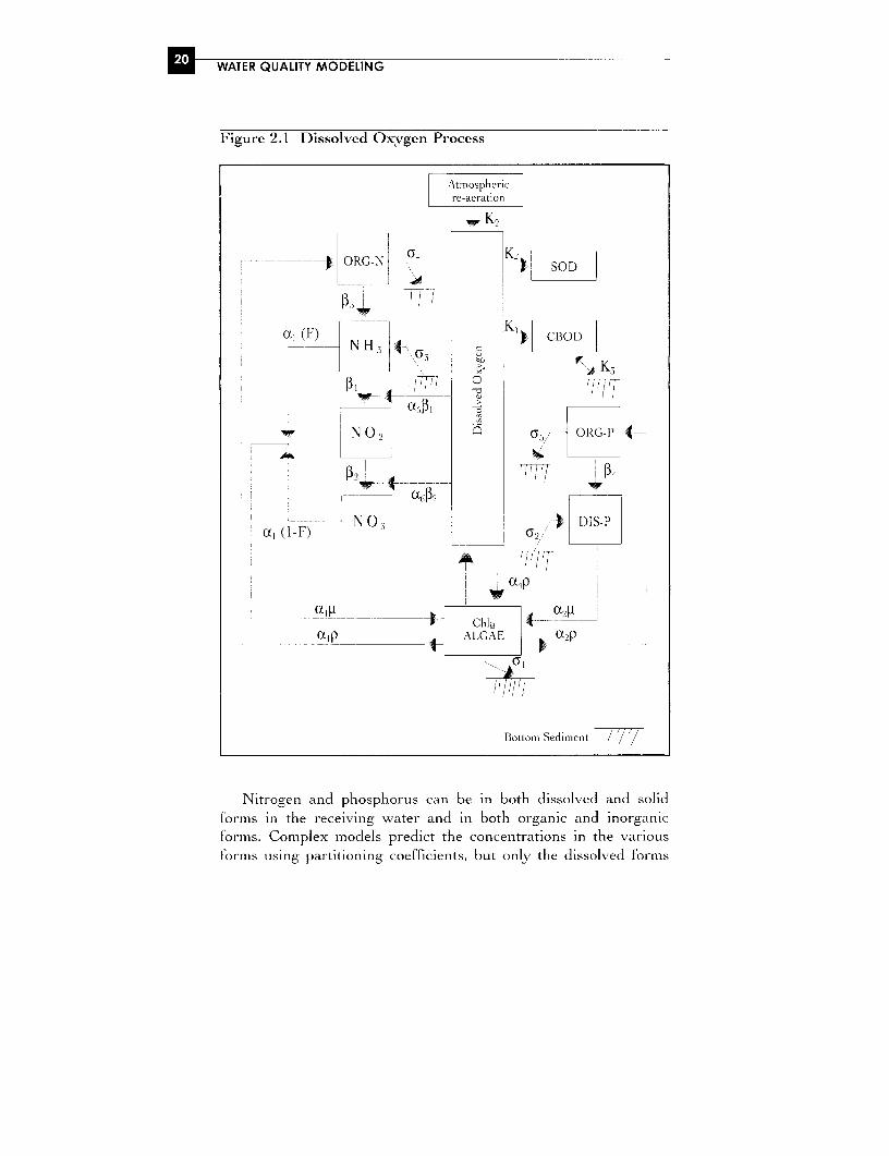
The DO kinetics in a natural water body is complex. Figure 2.1shows the dissolved oxygen sources (external supply, photosynthe-sis, surface re-aeration, denitrification) and sinks (BOD), water col-umn and sediment oxygen demand (SOD),respiration, andnitrification). Most of these processes are biological and occur over
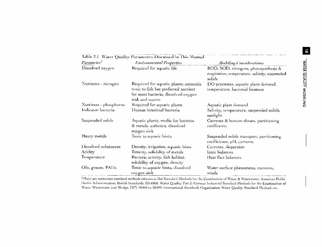
Talble 2.1 W\ater Quality P~arameters D)iSCLIsSed in Th'Iis ManuLal
eler Li~~Ftil oi'rnnelita/ I )cprtie iThode/inq L•aizsideration,"
Dissolved oxygen Required for aquatic life BOD, SOD, nitrogens, photosynthesis & -
respiration, temperature, salinity, suspended0
solids >Nutrients - nitrogen Required for aquatic plants; ammonia DO processes, aquatic plant demand,
toxic to fish but preferred nutrient temperature, bacterial biomassfor m-ost bacteria; dissolved oxygen 0
nisink and source
zNutrients - phosphorus Required for aquatic plants Aquatic plant demand pIndicator bacteria Human intestinal bacteria Salinity, temperature, suspended solids,
sunlightSuispended solids Aquatic plants, media for bacteria Currents & bottom shears, partitioning
& metals, asthetics, dissolved coefoicentsoxygen sink
Heavy metals Roxic to aquatic biota Suspended solids transport, partitioningcoefficients, pll, currents
Dissolved substances Density, iprigation, aquatic biota Currents, dispersionAcidity Toxicity, solubility of metals Ionic balancesTemperature Bacteria actilvity, rish habitat, Heat flux balances
solubility of oxygen, densityOils, grease, PAHs Toxic to aquatic biota, dissolved Water surface phenomena, currents,
oxygen sink windsThere are numerous standard methods references like Standard Methods for the Examination oliWater & Wastewater, Anoerican PilicHealth Administration; British Standards, o iS 6068, Water Quality Part 2; German Industical Standard Methods for the Examination ofWater, Wastewater and Sludge, DtIN s8404 to 38409; International Standards Organization Water Quality Standard Method; etc.

WATER QUALITY MODEL STRUCTURE AND PROCESSES U
a period of time; the biological process rate is very sensitive to tem-perature.
DO is modeled as oxygen deficit, or the difference between theDO concentration and the concentration of the DO when the wateris saturated with DO. The saturation concentration is a function ofboth the temperature and the salinity. Saturation concentrations arenormally available in the model manual or other standard references(APHA, 1998).
The DO concentration is a function of numerous physical andbiochemical processes. DO processes modeled are those shown inFigure 2.1. The model user has the option of omitting processes thatmay not be important in a particular application. For example, SODis not important for rocky substrates, and photosynthesis and respi-ration are normally not factors in fast-moving rivers or receivingwaters with high turbidities. Many of the processes in the DOequation are difficult to measure; consequently, these processesare imprecise. For example, the precision of the biochemical oxygendemand is 10-20 percent; re-aeration, 20-30 percent; photosynthesisand respiration, 10-20 percent; and sediment oxygen demand, 10-20percent. Simplifying the model by omitting processes that areknown to be very imprecise can improve the precision of themodel predictions.
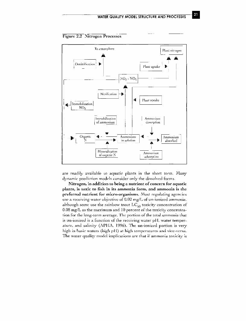
Nutrients. In water quality studies, only the vegetation nutrientsnitrogen and phosphorus are considered because domestic waste-waters have high concentrations of nitrogen and can have high con-centrations of phosphorus. Aquatic plants are part of the DOprocesses shown in Figure 2.1. Phytoplankton (microscopic free-float-ing plants) are the foundation of the aquatic biota in the receivingwater as the food supply for zooplankton. Without nutrients, aquaticorganisms cannot exist; however, an excess of phytoplankton bio-mass can cause receiving water quality to degrade, primarily in theoxygen demands for the decay of expired phytoplankton bio-mass.The ideal molecular ratio for phosphorus:nitrogen:carbon for plantgrowth is about 1:10:40. Phosphorus, nitrogen, and carbon can bemeasured with a precision of <10 percent. In general, aquatic plants inestuaries tend to be nitrogen-limited. High concentrations of nutrients,particularly nitrogen, can result in nuisance growths of aquatic plantsand species. The nitrogen processes in the receiving water are shownin Figure 2.2, and the phosphorus processes in Figure 2.3.
fl WATER QUALITY MODELING
Figure 2.1 Dissolved Oxygen Process
Atmosphericre-aeration
4 K2
--- --- ORG-N -) SOD
u (F) K
NH %4 CBOD c'rr~, K3
N02~~~
, *(X4p *
w N 2 (37 OGP
_w_ _ °t!p_ -- i- Chla--lO!lp ALGAE 0 2P
| ~~~~~~~~~~~~Botiom Sediment///
Nitrogen and phosphorus can be in both dissolved and solidforms in the receiving water and in both organilc and inorganicforms. Complex models predict the concentrations in the variousforms using partitioning coefficients, but only the dissolved forms
WATER QUALITY MODEL STRUCTURE AND PROCESSES U
Figure 2.2 Nitrogen Processes
To atmosphere l
Denitrification ~~~ Plant uPtake mtrge
|cNitrification )
FPlant uptakeImmobilization
Immo.billization Ammonium._of ammonium desmmoptiun
Organic - Ammonium | - AmmoniumN - -* in solution -- absorbed
Ak
| lineralizationof organic N adron
are readily available to aquatic plants in the short term. Manydynamic prediction models consider only the dissolved forms.
Nitrogen, in addition to being a nutrient of concern for aquaticplants, is toxic to fish in its ammonia form, and ammonia is thepreferred nutrient for micro-organisms. Most regulating agenciesuse a receiving water objective of 0.02 mg/L of un-ionized ammonia,although some use the rainbow trout LC50 toxicity concentration of0.08 mg/L as the maximum and 10 percent of the toxicity concentra-tion for the long-term average. The portion of the total ammonia thatis un-ionized is a function of the receiving water pH, water temper-ature, and salinity (APHA, 1996). The un-ionized portion is veryhigh in basic waters (high pH) at high temperatures and vice-versa.The water quality model implications are that if ammonia toxicity is

-- ~~~~~~~~~~~~~ cPlant m
phosphorus (P) I
Planltuptake 0I
vl r~~l
DesorptionI
Phosphate phosphateimmobilization
Organic in ~~~~~~~Phsopto Phiosphate
Organic P osl absorbed
p~~~~~~~~~~~~~~~~~~~~~~~~~~~~~~~~~~~~~~~~~~~~~~~~~~~~~~~~~~~~~~~~~~~~~~~~~~~~~~~~~~~~~~~~~~~~~~~~~~~~~~~~~~~~~~~~~~~~~~~~~~~~~~~~~~~~~~~~~~~~~~~~~
Organic P Adsorptiomineralization phsat

WATER QUALITY MODEL STRUCTURE AND PROCESSES C
to be predicted, it is necessary to predict the pH and temperatureand salinity in marine environments as well as total ammonia con-centrations.
pH is difficult to model and predict. In most instances, pH mustbe measured in the receiving water, and statistical values for the pHare used to determine the un-ionized portion of the ammonia. Theperiod that most affects the ammonia prediction is when the receiv-ing water temperatures and pH are the highest and when the salin-ity is the lowest. Furthermore, because many agencies specifydifferent concentrations for instantaneous prediction and averagesover a period of days, appropriate time-averaged concentrationsmust be predicted.
Phosphorus is an aquatic plant nutrient. In natural freshwaterreceiving waters, phosphorus is frequently the nutrient that limitsexcessive aquatic plant growths. Domestic wastewaters are a sourceof phosphorus for the receiving water and can cause excessiveaquatic plant growths, which will result in a degraded water quality.
Predicting the nutrient concentrations in receiving water usingwater quality models requires that the phytoplankton bio-mass andspecies as well as the macrophyte bio-mass be known. Because of thepatchiness of phytoplankton bio-mass and the kinetics of the bio-mass (Palmer, 1981: Harris, 1980: Denman et al., 1977), quantifyingit requires an extensive field measurement program. Furthermore,using bio-mass measurements in the water quality prediction modelsintroduces more imprecision.
Indicator bacteria. The density of indicator bacteria is used as ameasure of the presence of domestic wastewater in the receivingwater and, consequently, the public health risk associated withhuman contact with these waters. The presence of domestic waste-waters has historically been determined by measuring a group ofintestinal bacteria. Originally, a total coliform determination wasdeveloped. This test was subsequently replaced with a fecal coliformand E. coli test that was found to be more specific for the presence ofintestinal bacteria. "Although E. coli is undisputed as the fecal indi-cator of choice, some of the fecal coliform tests used will also enu-merate Klel,i'ella spp fecal sources" (NHW, 1992). Numerousattempts to define the bacterial density objective using epidemiolog-ical studies have met with with mixed results (see NHW, 1992 for a
WATER QUALITY MODELING
good discussion of bacteria indicators). Most regulating agencies usegeometric mean density objectives of between 100 cfu/lOOmL (cfu =colony forming units) to 500 cfu/lOOmL (about 1 part sewage:1 00,000 parts water) for recreational waters and for drinking water0 cfu/lOOmL fecal coliforms and < 10 cfu/lOOmL total coliforms.
For recreational waters, model predictions must be suitablefor the applicable receiving water quality objective, typically ageometric mean of 5 to 10 samples. The precision and accuracy ofsampling, transporting, and measuring bacterial densities areabout logI0 0.2 to log1 0 0.35
In receiving waters, the bacterial cells are normally attached toorganic flocs or suspended solids (see, for example, Palmer & Bur-relle, 1996); consequently, the densities can vary between samples.Furthermore, these intestinal bacteria cannot survive for very longin natural water bodies, particularly if the salinities are high. Themortality rate of the bacterial cells is a function of many factors andgenerally not universal. The mortality rate is site-specific, and typi-cally a 90 percent mortality occurs in 3 to 6 hours in marine waters(Palmer & Dewey, 1984) and in 12 to 30 hours in fresh waters.Mortality rates are normally measured by releasing and tracking abacterial seed, frequently mixed with a visible dye tracer, eitherdirectly in the receiving water or in containment bags in the receiv-ing water.
Most recreational indicator bacteria objectives are defined as thegeometric mean of 5 to 10 samples over a period of time. Regulatingagencies also frequently specify the field sampling methods to reducevariability in the samples. The model predictions should be geomet-ric mean densities, and models that predict organic floc and sus-pended solids transport are better for indicator bacteria. Theprediction models for indicator bacteria normally consist of trans-port, dispersion, and mortality. Transport and dispersion can be pre-dicted with precision on the order of 50 percent, provided that thereceiving water is not very dynamic. The mortality rate can cause thepredictions to be imprecise, particularly in salt water receivingwaters. In situ measurements of mortality are difficult unless a largebacterial source exists (Gannon and Busse, 1989; Palmer, 1984: andSpringthorpe et al., 1993). The method for determining the densitiesof the indicator bacteria by culturing also introduces imprecisioninto the measurements, which affects the prediction model calibra-
WATER QUALITY MODEL STRUCTURE AND PROCESSES
tion and verification. Typically, the log standard deviation for thedensities of indicator bacteria in the laboratory for split (three) sam-ples is between 0.15 and 0.25 (Palmer, 2000). An extensive qualityassurance and control program is necessary for indicator bacteriamodel predictions.
Suspended solids. Suspended solids can be inorganic or organic.Both are important in determining whether aquatic plant productiv-ity and/or aesthetics will be affected. Most of the heavy metals likecopper, zinc, lead, cadmium, and iron are associated with the veryfine (cohesive) sediments. Indicator bacteria attach themselves tosuspended solids, particularly the organic flocs. Similarly, organiccompounds like pesticides and herbicides tend to combine withorganic flocs. The transport and fate of suspended solids areimportant in determining the concentrations of metals, bacteria,and organic substances in the receiving water.
Suspended solids measurement is a mass measurement and assuch generally underestimates the importance of the organic flocsand plankton bio-masses. The turbidity measurement, which is alight transmittance measurement, is frequently used in receivingwaters. The interpretation of Secchi disc data is extremely difficult(Effler, 1985) and probably should be avoided in quantitative inter-pretations. There is no rigorous relationship between suspendedsolids and turbidity, although there is a general correspondenceunless the plankton or organic tloc bio-masses are large.
Domestic wastewaters have high concentrations of suspendedsolids. Typically, raw wastewaters have suspended solids concentra-tions of 100 to 200 mg/L (Metcalf & Eddy, 1992), which treatmentsystems can reduce to 10 to 50 mg/L. Receiving water objectives aretypically expressed as a percentage increase (5 to 10 percent) overnaturally existing conditions. For instance, the characteristics of theorganic flocs are functions of the floc size, which is determined bythe physical shear processes in the receiving water. Physical shear isdifficult to predict in receiving waters. In general, the better sedi-ment dynamics models use sedimentation velocity, resuspensionvelocity, and transport velocities, and it is extremely important thatsite-specific field data be used in the predictions to improve theirprecision. Predicting the receiving water suspended solids con-centrations and the suspended solids sedimentation is important
M KATER QUALITY MODELING
in a model; however, predicting these processes for the very smallcohesive particles and the organic flocs is difficult and requirescomplex models.
Metals. Metals are associated primarily with the suspended solids.High concentrations of metals are toxic to aquatic life, with thedissolved form being the most toxic. The metals of greatest concernare copper, cadmium, zinc, lead, mercury, cyanide, chromium,nickel, arsenic, and iron, with the lowest concentration objectives formercury at 0.0002 mg/L, for cadmium at 0.004 mg/L, for copper at0.015 mg/L, and for cyanides at 0.005 mg/L. Normally, the concen-trations in domestic sewage are small and of little concern; however,if small industries such as metal shops, plating shops, and paintshops are connected to the domestic sewage system, metals can be aconcern in domestic sewage. Because the metals are associatedwith suspended solids, these metals can accumulate in the receiv-ing water sediments and have a negative long-term effect on thereceiving water and should be predicted in water quality models.Water quality prediction models must effectively predict the sus-pended solids transport and fate processes if metal concentra-tions are to be predicted in the receiving water.
Dissolxed substances. Dissolved nutrients and metals have beendiscussed in the preceding text. Other dissolved substances of inter-est in the receiving water are salinity, hardness, and salts. The totaldissolved solids concentration is measured as conductivity with anaccuracy and precision of 1 to 2 percent, and because temperatureaffects the conductivity measurement, the conductivity is given for astandard temperature. The mass of the various ions and cations canalso be measured with an accuracy of 4 to 5 percent.
Large changes in the natural salinity of the receiving watercannot be tolerated by the existing biota. Consequently, regulatingagencies generally restrict changes in salinity to less than 10 percentof existing levels. In marine environments, natural salinity is sea-sonal; therefore, model predictions should be for the season of lowsalinity. Salinity of more than 125 mg/L is also a concern in fresh-water receiving waters if the water is to be used in irrigation. Sodiumof more than 20 mg/L is also a concern for irrigation and drinkingwater. Hardness is a concern because it affects the toxicity levels for

WATER QUALITY MODEL STRUCTURE AND PROCESSES U
fish if metals and unionized ammonia are elevated in the receivingwater.
Dissolved substances in the receiving water are diluted by bulkmixing and dispersion; consequently, these concentrations can bepredicted well with most water quality models. The precision andaccuracy for the total dissolved solids concentration predictions aresimilar to the precision and accuracy for the transport and dilutionmodels. Conductivity data are useful in estuaries where the conduc-tivity is on the order of 32,000 umhos/cm for salt water, municipaleffluent is at 200 to I 000 umhos/cm, and the fresh water has a nearlyzero conductivity level. Conductivity is used extensively in estuariesto quantify the fresh water fraction at any location in the estuary.
Total dissolved solids are measured as conductivity with an accu-racy and precision of about 1 to 2 percent; however, conductivity isa function of temperature and must be given for standard tempera-tures. In modeling, conductivity data are useful for mass balancesin estuaries and in the vicinity of wastewater discharges.
Acidity. The pH in the receiving water is an important parameterfor chemical reactions and toxicity. Acidic pHs permit metals togo into solution. The pH is also important in the bicarbonate equi-librium in fresh waters, and it affects the levels of most toxicants forfish. Generally, the higher the pH, the less toxic toxicants are to fish.pH is not predicted by most water quality models and must bemeasured in the field. This can be done with a precision of 0.1 usingstandard pH meters.
Temperature. Temperature is an inmportant factor in the chemicalreactions and biological activity in the receiving water. Tempera-ture is also an important parameter for fish habitat where the watertemperature maximums and temperature ranges must be within spec-ified limits for specified seasons. The seasonally acceptable range andlimits are defined by the by life cycle of the different fish species.Water temperatures are predicted well by many water qualitymodels and can be easily measured with a precision of about 0.1 °C.In estuaries, it may be necessary to measure the temperature withgreater precision using more sophisticated equipment. Existing waterquality models are capable of predicting water temperature with anaccuracy and precision of about 3 to 5 percent.
El WATER QUALITY MODELING
Oils and grease. Municipal wastewaters are a source of oils andgrease. Most regulating agencies specify that surface grease andoils be undetectable by sight or smell (<0.1 mg/L). Both are pres-ent in most domestic sewage and must be removed by treatment.Oils and grease are not predicted in most water quality models butcan be predicted using the oil spill prediction models. Measurementsof oil and grease concentrations have a precision on the order of15 to 20 percent. For the oil spill models to be precise, extensivesite-specific data are required. Seldom are these data available; con-sequently, oil spill models typically have a precision of 25 to 50percent.
Polycyclic aromatic hydrocarbons (PAHs). PAHs are toxic toaquatic life at low concentrations (0.1 to 10 ug/L). In mostinstances, the hydrocarbons are buoyant in the receiving waterand require special oil spill or surface film water quality modelsthat have a precision rate of 25 to 50 percent (unless extensivesite-specific data are available). Hydrocarbons that are associatedwith suspended solids can be predicted using water quality modelsthat predict the suspended sediment transport and fate. Any modelwill have difficulty predicting PAH concentrations at the lowobjective levels; consequently, PAHs can only be predicted quali-tativelv.
RECEIVING WATER PROCESSES
When a substance is discharged to a receiving water, manv differentreceiving water processes move the substance, dilute it, and changeit. These processes are the basis of all water quality prediction mod-els. Some processes are easier to model than others, and theprocesses are not independent of each other. One of the majorstrengths of water quality models is that the model integrates theinteraction of these processes.
Physical processes. Dilution is simply the mixing of a volume at oneconcentration with another volume at a lower concentration. Simplebatch computation produces the resulting concentration. For contin-uous flows, batch computation can be done over a period of time.This computation is frequently carried out as a first-order approxi-

WATER QUALITY MODEL STRUCTURE AND PROCESSES i
mation or as a means of confirming more complex model predictions.It is sometimes called a "reality check."
Dispersion refers to the mixing processes that occur as a result ofeddies within the fluid, differences in velocity in different areas in thefluid (sometimes called the shear), and gradients of concentration.Dispersion is normally expressed as a temporal constant (and fre-quently as a spatial constant) associated with the concentration gra-dient terms in the mass balance equation. In fact, the dispersioncoefficient varies with time (Alsaffar, 1966; Okubo, 1971), so themost appropriate dispersion coefficient is selected for the model. Dis-persion coefficients in a water quality model are frequently adjustedin the calibration of the model. For some unexplained reason, themodel calibration dispersion coefficient may be very different fromsite-specific field measurements. In these situations, the model cali-brated dispersion coefficient should be used in the prediction process.
Advection is the (velocity multiplied by concentration) term inthe mass balance equation. It is generally referred to as the mass
transport in the direction of the velocity. In models, advection is a
complex process because both the velocity and concentration are
time and spatial variables.Tides affect water levels, which changes the volume of water;
therefore, there is more dilution water during high tides and less dur-
ing low tides. But there are other considerations for a freshwater
waste discharge to marine water. The difference in densities between
the freshwater effluent and receiving water reduces the rate of mix-
ing of the two waters. If freshwater sources exist in the coastal
region, salinity gradients can exist; when that is the case, the differ-
ences in water density can generate density-difference-driven circu-
lation in the coastal waters. In long estuaries, the tidal effects on
water quality can be very complex because of the temporal, spatial,and seasonal variability of the tidal processes combined with the
variability of discharges.
Most river flows vary seasonally and can have shorter-period
variations associated with rainfall. River flow is an important water
quality parameter that most water quality models treat as a spatial
and temporal variable.
Currents in the receiving water can be generated by winds, tides,density, thermal differences, or river flows. These currents and theirspatial and temporal variations produce dilution and dispersion in
E WATEgQULITY MODELING
the receiving water. In a narrow river, the currents are directlyrelated to the river flow, but in wide rivers, lakes, estuaries, andmarine coastal regions, the currents are much more complex. Cur-rents are vectors (speed and direction) which normally vary withtime, location, and season.
Buoyancy, both positive and negative, is the difference in densitybetween the effluent and the receiving water. The largest differences
in density occur for freshwater discharges into a salt water receiving
water; however, the density differences between effluents at temper-
atures different from the freshwater receiving water are also a con-
cern. The density differences reduce the rate of the mixing of the
effluent and the receiving water, resulting in higher concentrations in
the receiving waters.
Density stratification in receiving waters is a seasonal phenom-
enon in lakes, reservoirs, and marine coastal regions and is a perma-
nent feature in estuaries. The density depth stratification reduces the
rate of mixing with depth and changes the physical transport
processes in the various depth layers of the receiving water. Receiv-ing water depth stratification is an important factor in determining
water quality in the receiving water and, if it exists, must be
addressed in the water quality models. In general, three-dimensional
models are avoided because of the difficulty in calibrating these mod-
els. Specialized models like the oil spill models have been developed
for buoyant contaminants in the receiving water, and some two-
dimensional models can be used in the depth for density stratifica-tion and in the downstream dimensions.
Suspended sediment kinetics in the receiving water is the mainmechanism for the transport of bacteria, heavy metals, and organiccontaminants. Both the organic flocs and inorganic suspended cohe-sive solids are important. A water quality model for sediment kinet-ics should include settling, transport, resuspension, and partitioning.Sedimentation velocity is a function of the particle size and densitydifference between the particle and the receiving water. Resuspen-sion is a function of the physical shear at the bottom, type of bottom,
and particle size defined by mobility and transport parameters (Ack-ers & White, 1973; Yalin, 1977; Van Der Kooij et al., 1991). Parti-
tioning coefficients that identify the portion of the metal in both thesolid and dissolved states are different for the different metals, con-centrations of suspended solids, and their porosity. Sediment kinet-
WATER QUALITY MODEL STRUCTURE AND PROCESSES
ics is so complex that few water quality models address them in acomprehensive manner. Most models address only the sedimentationand partitioning processes.
Surface processes. The most important surface process for gen-eral water quality modeling is re-aeration because the two mainmechanisms for supplying oxygen to receiving water are surface re-aeration and photosynthesis. Surface re-aeration in receiving watersis a complex process that is a function of the surface area, turbu-lence, wind climates, dissolved oxygen concentrations near the watersurface, and temperatures of the air and fluid. Surface re-aerationcan be measured by injecting a gas like propane into the receivingwater and measuring the escape of this gas. However, because of thecost of these measurements and the number of measurementsrequired for all the different conditions, re-aeration is normallydetermined by using empirical relationships based primarily on fluidvelocity and depth of the receiving water. Mlost models allow theuser to select the relationship from a range of options. Frequently,re-aeration is used as a calibration variable.
Volatilization refers to the changing of a substance from a liquidto gaseous state at the liquid interface. The process is a function ofHenry's Law, transfer coefficients and concentrations (Lewis &Whitman, 1924; Gowda & Lock, 1985). Volatilization is an impor-tant process for organic contaminants of concern. For generalwater quality modeling, the main concerns are PAHs, and their fatein the receiving water is approximated by a single factor in the oilspill models.
Atmospheric deposition is an important process for nutrients,particularly for phosphorus in freshwater lakes. Most water qualitymodels do not consider atmospheric deposition as a process in themodel, though it may be included in models as a non-point sourceusing locally measured deposition rates per area or literature deposi-tion rates.
Biochemical processes. Chemical processes occur during a shortperiod of time, whereas biological processes occur over a muchlonger period.
Dissolved oxygen is essential for most aquatic biological life.DO processes are designated as either sources or sinks which when
Ex WATER QUALITY MODELING
summed result in the DO concentrations in the receiving water.These processes are shown in Figure 2.1. Because all of the DOprocesses are biological except for surface re-aeration, time isrequired for them to take place. The rates of these processes arealso functions of temperature. In general, biological activityincreases with temperature. One of the DO sinks is the biochemicaloxygen demand, which is measured over a five-day period accord-ing to methods in various publications (APHA, 1996; ASTM Annual( 11.01 &' 11.02; British Standards, British Standards Institute,WaTzter- Qzal/iy BS-6068). When large amounts of BOD are dis-charged into a receiving water with a long residence time, it is oftennecessary to measure BOD for periods longer than five days,
referred to as "the ultimate BOD" (National Council, 1982, 1986).
Atmospheric re-aeration and sediment oxygen demand (Figure 2.1)
are difficult to measure in the field, and empirical methods are fre-quently used in models for these processes. The empirical methods
for re-aeration are based on flow characteristics and depth, and for
sediment oxygen demand are based on the organic carbon concen-trations in the sediments. Using these empirical methods in water
quality models affects the precision and accuracy of the model pre-
dictions.
Phosphorus is a necessary nutrient for the growth of aquatic
flora (Figures 2.1 and 2.2). The natural sources of phosphorus are
generally limited; consequently, natural freshwater systems often
have little phosphorus. Domestic sewage, on the other hand, often
contains large amounts of phosphorus, and discharges of untreated
domestic sewage can change the nutrient balance in the receiving
water. As aquatic flora require only small amounts of phosphorus,
treatment systems must remove the phosphorus to concentrationsto about one mg/L to control the eutrophication in the receiving
water.Nitrogen is a necessary nutrient for the growth of aquatic plants
(Figures 2.1 and 2.3). Domestic sewage (typically 25 to 30 mg/L of
total organic nitrogen) and animal wastes contain high concentra-
tions of organic nitrogen, which can cause eutrophication in the
receiving water. (The ideal molecular weight ratio of nitrogen to
phosphorus is about 10:1; therefore, the receiving water is more sen-
sitive to phosphorus discharges than to nitrogen discharges.) How-
ever, because much of the nitrogen is in an ammonia form, it exerts

WATER QUALITY MODEL STRUCTURE AND PROCESSES
a high oxygen demand on the receiving water. Furthermore, highconcentrations of ammonia are toxic to fish.
Photosynthesis and respiration of aquatic flora are important inDO balance in the receiving water. The photosynthesis and respira-tion processes are shown in Figure 2.1. In the water quality models,the phytoplankton growth rates are expressed in equations that haveterms for light, extinction coefficients, depth, temperature, and car-bon:chlorophyll a ratios. Another approach to quantifying photosyn-thesis and respiration is to measure DO concentrations andtemperature at a fixed point for a period of 30 hours. Data collectedfrom these measurements can be used to quantify photosynthesisand respiration.
Bio-mass transfers in the aquatic food web system, includingdetritus. Most natural receiving waters contain suspended solids,which consist of inorganic particles-principally clay particles, phy-toplankton and zooplankton, and organic flocs -referred to as detri-tus. The detritus is consumed by zooplankton and fish and ultimatelyreturned to the receiving water as a waste product. The detritusmay have high bacterial densities, heavy metal, and other organiccompound concentrations which may be returned to the receivingwater or remain in the zooplankton and fish. Bio-mass transfers inthis manner can be important when predicting the concentrations ofwater quality parameters in the receiving water.
Indicator bacteria are intestinal bacteria from warm-bloodedanimals; they cannot normally survive in natural receiving waters.Their mortality rate in the receiving water is referred to as T90,which is the time required for an order of magnitude reduction in thedensity of the bacteria. In a marine receiving water, the T90 is typi-cally 3 to 6 hours; in freshwaters it is 12 to 30 hours. The T90 is func-tion of temperature, particle association, sunlight, and other factors.T90 can be measured in the field using various methods, but in mostinstances, literature T9Os or a range of T9Os are used in water qual-ity models with some site verification data. Sometimes it is best toselect a T90 value that is too large so that the predictions will be con-servative.
Sediment water interactions are important for the water qualityparameters that are associated with suspended solids like indicatorbacteria, heavy metals, and organic substances of concern. The por-tion of the water quality parameter in a dissolved form and associ-

fl WATER QUALITY MODELING
ated with suspended matter is generally defined by the partitioncoefficient. This coefficient is a characteristic of the substance beingmodeled. Most water quality models predict total concentrations,which consist of the dissolved and suspended solids components,with the portion in each state determined from the partition coeffi-cient.
General Prediction Confidence
The physical and biochemical processes discussed in the precedingsections can be measured and modeled with varying degrees of con-fidence. It is helpful to list what can be measured in the field andwhat is difficult to measure. Water quality parameters that can beeasily measured in the field with some precision are:
* physical parameters like position, depth, temperature, salinity, turbid-ity, particle size, and sediment-settling velocities;
* chemical parameters like concentrations of most substances, includingdissolved oxygen and suspended solids, and pH; and
* biological parameters like bacterial densities, phytoplankton and zoo-plankton bio-masses, and fish species and populations.
Water quality parameters that are difficult to measure in the fieldare:
* physical parameters like bottom roughness, circulation patterns, resus-pension of sediments, surface re-aeration, partition coefficients, trans-port and fate of organic flocs and cohesive sediments, and atmosphericloadings;
* chemical parameters like sediment oxygen demand and volatilization;and
* biological processes like indicator bacteria mortality and detritus bio-mass recycling.
In most instances, processes that are difficult to measure aredefined by empirical methods or through literature values for similarreceiving water. If empirical methods or literature values are used,

WATER QUALITY MODEL STRUCTURE AND PROCESSES U
the model prediction precision is affected. The process of definingthe precision and accuracy of models is based on the quality assur-ance and quality control in both the field data collection and analy-sis and modeling process.


| ! - ~C H A P T E R 3
Some Coninionly UsedModels
n overview of water quality models was presented in Chap-ter 1. There is a general structure in the water quality mod-
k.hels being used today. This structure is discussed in thischapter. Understanding this structure will assist a potential modeluser in evaluating the characteristics of any model. Most of themodels have three parts, which are discussed in the following text.The model user in many cases can omit processes that may not beimportant in a particular application. These simplifications are dis-cussed. Equations are presented to show the required user inputsto the model for the different processes in the receiving water.While it is true that every model has some unique characteristics, ageneral common structure exists in the models. This commonstructure consists of three parts: 1) the hydrodynamic/hydrologicalpart, 2) the mass balance part, and 3) the receiving water processpart. Much of the following discussion is based on the informationcontained in the various model manuals that are discussed in theAppendix.
HYDRODYNAMIC MODEL
The hydrodynamic characteristics, namely the spatially and tempo-rally varying velocity vectors and water levels, can be determined bysolving the following equations, shown below.
Receiving Water Equation of Motion
The equation represents the change of local inertia and rate ofmomentum change.
37

A WATER QUAULTY MODELING
a&,' - -(, at n (1)a,~ ~ + ,at axi
where l = velocity in the i direction
t = time
xi = distance in the i direction
n = gravity, friction, and wind acceleration
Gra 'ity = _g aH (2)ax.
where H = depth
g = acceleration resulting from gravity
Frictu7/z = -g- (U. U. (3)
where n = bottom friction
R = hydraulic radius = wetted area/perimeter
Win=Ld a• W2 cos (D (4)R p1
where = surface drag coefficient
pP,,. p= density of air and water
W = wind velocity at 10 m
0 = wind angle
Receiving Water Equation of Continuity
The continuity equation is the time-varying water mass balance rela-tionship, including water depth.
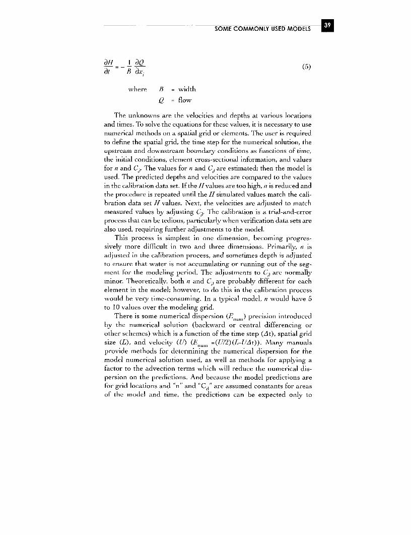
SOME COMMONLY USED MODELS
aH 1 aQat B ax, (5)
where B = width
Q = flow
The unknowns are the velocities and depths at various locationsand times. To solve the equations for these values, it is necessary to usenumerical methods on a spatial grid or elements. The user is requiredto define the spatial grid, the time step for the numerical solution, theupstream and downstream boundary conditions as functions of time,the initial conditions, element cross-sectional information, and valuesfor n and Cd. The values for nj and Cd are estimated; then the model isused. The predicted depths and velocities are compared to the valuesin the calibration data set. If the Hvalues are too high, n is reduced andthe procedure is repeated until the H simulated values match the cali-bration data set H values. Next, the velocities are adjusted to matchmeasured values by adjusting C). The calibration is a trial-and-errorprocess that can be tedious, particularly when verification data sets arealso used, requiring further adjustments to the model.
This process is simplest in one dimension, becoming progres-sively more difficult in two and three dimensions. Primarily, n isadjusted in the calibration process, and sometimes depth is adjustedto ensure that water is not accumulating or running out of the seg-ment for the modeling period. The adjustments to Cd are normallyminor. Theoretically, both ni and Cd) are probably different for eachelement in the model; however, to do this in the calibration processwould be very time-consuming. In a typical model, ti would have 5to 10 values over the modeling grid.
There is some numerical dispersion (Enum) precision introduced
by the numerical solution (backward or central differencing orother schemes) which is a function of the time step (At), spatial gridsize (L), and velocity ([/) (Enum =(U/2)(L-UAt)). Many manualsprovide methods for determining the numerical dispersion for themodel numerical solution used, as well as methods for applying afactor to the advection terms which will reduce the numerical dis-persion on the predictions. And because the model predictions arefor grid locations and "n" and 'Cd" are assumed constants for areasof the model and time, the predictions can be expected only to

WATER QUALITY MODELING
match measured data sets approximately. The velocities and waterdepths predicted from these two equations are used as inputs to thenext model part.
The only model simplification possible for the hydrodynamic partof a model is to assume steady-state conditions and reduce thedimensions to twvo or, if possible, one. There are a couple of tricksthat can extend the capabilities of simplified models. Steady-state
models can be run repeatedly for different conditions to simulatetime-variable conditions, and in some instances the model dimen-sions can be reduced to one dimension by using streamlines as anaxis.
MASS BALANCE
Discharged Substance Mass Balance Equation
A general mass balance equation is the time-varying conservation ofthe mass of a substance dissolved or suspended in the water.
ac - a-TL•) + a (E dC) + (6)at axta axt, a.Jx
where C = concentration
l,T = velocity in direction i= distance in direction i
E. = diffusion coefficient direction i
S. = sources point and non-point, boundaryloading rate, atmospheric, kinetic trans-forms
In the general mass balance equation above, the first term on theright-hand side of the equation is referred to as the advection ortransport component, the second term is the dispersion component,and the last term is the sources and sinks.
The finite difference form of the mass balance equation for thenumerical solution consists of the following.

SOME COMMONLY USED MODELS U
Discharged Substance Transport Equations
Transport equations are used to represent the movement of a sub-
stance dissolved or suspended in the water.
AV= (fYoft, + precipitation - eaporatiwn) (7)
where V = volume
A( v) QC +- - Qp(D + - ,ACf + X RAC+ (8)
: (R (fDA(C n))) + XW + yVSk
where C = concentrationQ = flowQp = pore water flowf, ,/S = dissolved and solids fractions
W s = solids transport velocity
A = area
R = dispersive flow
R p= dispersive pore water flow
W7 = sources and sinks - point, non-point bound-
ary sources
S = kinetic transforms
Each parameter introduces another equation as shown below.
Pore Water Advection
___ =' C*'IDC (9)
where illf = mass of chemical

WATER QUALiTY MODELING
C = total chemical concentration
N = porosity
f = dissolved fraction of chemical
Q = pore water flow rate
Sediment Advection
H, aSi = __ DS, - (G'R + "'S) S$ (10)
where i sediment
j = water
H = depth
I = sediment concentration
[s )= deposition velocity
wR = scour velocity
s= sedimentation velocity in upper benthiclayer
The user can select any or all of the advection relationshipsabove. In all cases, the user must provide the segment interfacialareas, characteristic lengths, and segmentation. In addition, for thesediment advection, the sediment transport velocity and fractionabsorbed to sediment must be provided.
Similar mathematical relationships can be developed for the dis-persion terms. In these relationships, the user must provide the dis-persion coefficient as a function of time and, for the pore water, thedissolved fractions in the water and sediment.
In the mass balance part of the model, the user can add or deleteadvection or dispersion terms to suit a particular application of themodel. However, the addition of each term requires that the userdefine the appropriate coefficient for the model application. The nextmodel part is the receiving water processes.

SOME COMMONLY USED MODELS ]3
RECEIVING WATER PROCESSES
Dissolved Oxygen
The receiving water DO processes are shown in Figure 3.1. These
processes can be expressed in an equation as follows:
dt= K2(0 (t- 0)+ (a 3f - a 4p)Gn -K 1 L -K 4 /H- a5 N - a6 8N 2 (11)
where 0, 0° = DO and DO saturation concentration
(mg/L)
a13 = rate of oxygen production per unit of algal
photosynthesis (mgO/mgGn)
a4 = rate of oxygen uptake per unit of algal
respired (mgO/mgGn)
a5 = rate of oxygen uptake per unit of ammonia
nitrogen (mgO/mgA\)
a6 = rate of oxygen uptake per unit of nitrite
nitrogen (mgO/mgN)
mn = algal growth rate (temperature dependent)
(1/day)
r = algal respiration rate (temperature depend-
ent) (1/day)
G/l = algal bio-mass concentration (mg/L)
H = depth (m)
L = concentration of ultimate BOD (mg/L)
K, = BOD deoxygenation rate (temperature
dependent) (1/day)
K 2 = re-aeration rate (temperature dependent)
(1/day)
K 4 = SOD (g/m 2 day)
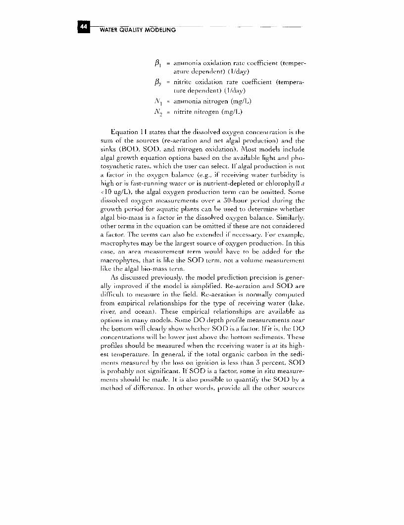
Cl WATER QUALITY MODELING
= ammonia oxidation rate coefficient (temper-
ature dependent) (I/day)
,2 = nitrite oxidation rate coefficient (tempera-ture dependent) (1/day)
N1 = ammonia nitrogen (mg/L)
A'9 = nitrite nitrogen (mg/L)
Equation 11 states that the dissolved oxygen concentration is the
sum of the sources (re-aeration and net algal production) and the
sinks (BOD, SOD, and nitrogen oxidation). NMost models include
algal growth equation options based on the available light and pho-tosynthetic rates, which the user can select. If algal production is not
a factor in the oxygen balance (e.g., if receiving water turbidity is
high or is fast-running water or is nutrient-depleted or chlorophyll a
<10 ug/L), the algal oxygen production term can be omitted. Some
dissolved oxygen measurements over a 30-hour period during the
growth period for aquatic plants can be used to determine whether
algal bio-mass is a factor in the dissolved oxygen balance. Similarly,
other terms in the equation can be omitted if these are not considered
a factor. The terms can also be extended if necessary. For example,
macrophytes may be the largest source of oxygen production. In this
case, an area measurement term would have to be added for the
macrophytes, that is like the SOD term, not a volume measurement
like the algal bio-mass term.
As discussed previously, the model prediction precision is gener-
ally improved if the model is simplified. Re-aeration and SOD are
difficult to measure in the field. Re-aeration is normally computed
from empirical relationships for the type of receiving water (lake,
river, and ocean). These empirical relationships are available as
options in many models. Some DO depth profile measurements near
the bottom will clearly show whether SOD is a factor. If it is, the DO
concentrations will be lower just above the bottom sediments. These
profiles should be measured when the receiving water is at its high-
est temperature. In general, if the total organic carbon in the sedi-
ments measured by the loss on ignition is less than 3 percent, SOD
is probably not significant. If SOD is a factor, some in situ measure-
ments should be made. It is also possible to quantify the SOD by a
method of difference. In other words, provide all the other sources
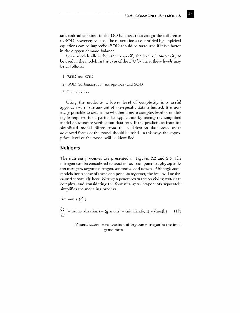
SOME COMMONLY USED MODELS l
and sink information to the DO balance, then assign the differenceto SOD; however, because the re-aeration as quantified by empiricalequations can be imprecise, SOD should be measured if it is a factorin the oxygen demand balance.
Some models allow the user to specify the level of complexity tobe used in the model. In the case of the DO balance, these levels maybe as follows:
1. BOD and SOD
2. BOD (carbonaceous + nitrogenous) and SOD
3. Full equation.
Using the model at a lower level of complexity is a usefulapproach when the amount of' site-specific data is limited. It is nor-mally possible to determine whether a more complex level of model-ing is required for a particular application by testing the simplifiedmodel on separate verification data sets. If the predictions from thesimplified model differ from the verification data sets, moreadvanced forms of the model should be tried. In this way, the appro-priate level of the model will be identified.
Nutrients
The nutrient processes are presented in Figures 2.2 and 2.3. Thenitrogen can be considered to exist in four components: phytoplank-ton nitrogen, organic nitrogen, ammonia, and nitrate. Although somemodels lump some of these components together, the four will be dis-cussed separately here. Nitrogen processes in the receiving water arecomplex, and considering the four nitrogen components separatelysimplifies the modeling process.
Ammonia (Cl)
aCl = (mineralization) - (growth) - (nitrification) + (death) (12)at
Mineralization = conversion of organic nitrogen to the inor-ganic form
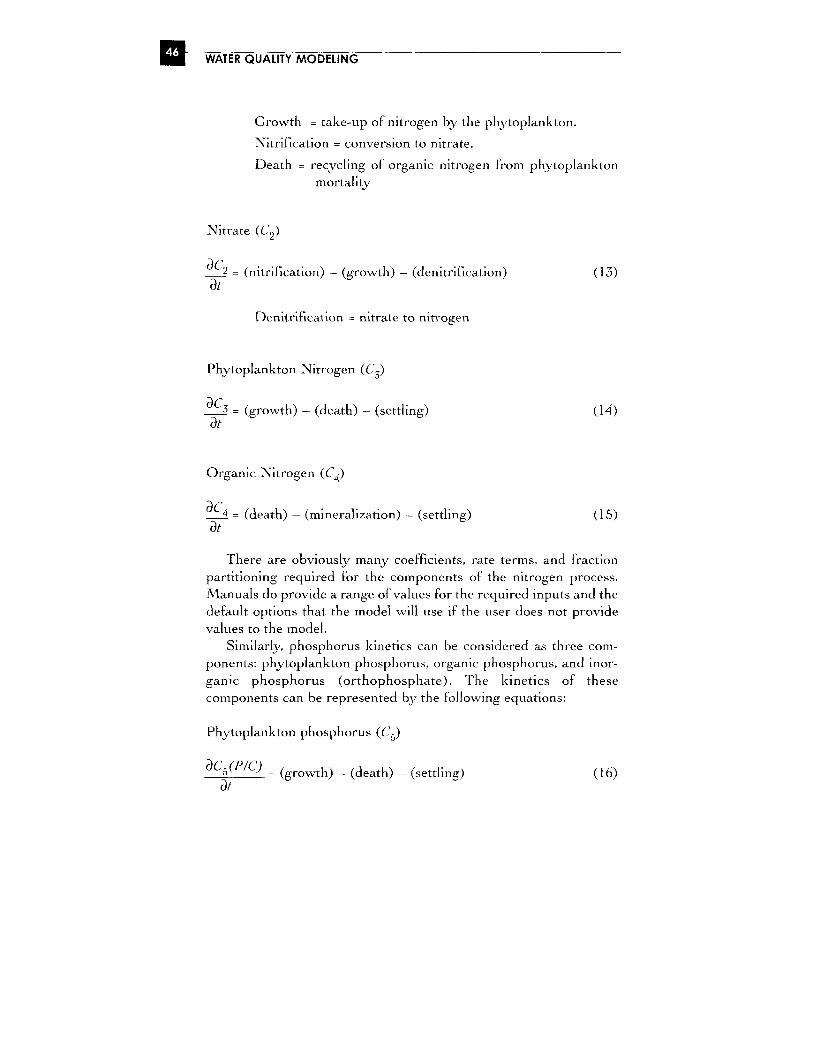
M WATER QUALITY MODELING
Growth = take-up of nitrogen by the phytoplankton.
Nitrification = conversion to nitrate.
Death = recycling of organic nitrogen from phytoplankton
mortality
Nitrate (C2)
aC9 - (nitrification) - (growth) - (denitrification) (13)
Denitrification = nitrate to nitrogen
Phytoplankton Nitrogen (C.)
aC 3 = (growth) - (death) - (settling) (14)at
Organic Nitrogen (C 4)
aC4 = (death) - (mineralization) - (settling) (15)at
There are obviously many coefficients, rate terms, and fraction
partitioning required for the components of the nitrogen process.
Manuals do provide a range of values for the required inputs and the
default options that the model will use if the user does not provide
values to the model.
Similarly, phosphorus kinetics can be considered as three com-
ponents: phytoplankton phosphorus, organic phosphorus, and inor-
ganic phosphorus (orthophosphate). The kinetics of these
components can be represented by the following equations:
Phvtoplankton phosphorus (C.)
C5 (P/C>) = (growth) - (death) - (settling) (16)at
SOME COMMONLY USED MODELS U
where P/C = phosphorus to carbon ratio in phytoplankton
Organic phosphorus (C6)
aC6 = (death) - (mineralization) - (settling) (17)at
Inorganic phosphorus (C7)
a_7 = (mineralization) - (growth) - (settling) (18)
Like the nitrogen component equations, coefficients, rate param-eters, and partitioning are required for the phosphorus processes.The range of values for these required inputs is provided in the man-uals, as well as the default options.
Some models allow the user to select the level of complexity forthe phytoplankton-nutrient kinetics similar to the DO balance. If thedata available for the site are limited, simpler models once again aremore appropriate, at least initially.
Heavy Metals
Heavy metal kinetics in a receiving water is complex because themetals can exist as soluble organic or inorganic complexes, sorbedonto organic or inorganic particles, and precipitate or dissolve. Allthe soluble components can be lumped into the dissolved term.WASP4 provides a modeling framework at four levels of complexity.Because the partitioning coefficients depend on the sorbent charac-ter of the suspended solids, there are no consistent partitioning coef-ficients. Site-specific measurements are required for heavy metalpredictions. The transport kinetics of suspended solids is included inthe mass balance part of the model (see equation 10); however, thepartitioning coefficients in this equation are for the liquid or solidstage. The partitioning of a substance between dissolved and sorbedfor equation 10 is predicted in this model component. If site-specificdata are limited at the site, simpler model configurations should be
i WATER QUALITY MODELING
used. For example, in the WASP4 model, the user can select from
the following levels of complexity for the metal predictions:
1. Specilf average concentration field by setting the initial conditions.
The solids concentrations will then influence the chemical partitioning.
2. Specify average concentration field and settling, deposition, scour, and
sedimentation velocities.
3. Simulate total solids by specifving loads, boundary concentrations, and
initial conditions, settling, deposition, scour, and sedimentation veloci-
ties.
4. Simulate three sediment types as in Level 3.
Heavy metals are associated primarily with the cohesive sedi-
ments, or organic flocs. In general, cohesive sediments will not settle
if the velocity is greater than about 12 cm/sec, and resuspension
occurs when the velocity is greater than 20 cm/sec. Knowing the crit-ical velocities and the velocities in the receiving water, it may be pos-
sible to simplify the sediment dynamics model.
Temperature
Many of the coefficients, rate parameters, DO saturation concen-
tration, and unionized portion of ammonia are temperature-
dependent; therefore, temperature must be predicted for the
receiving water. The generalized form of a temperature equation is
as follows:
a (A,aEi) a(A,UJT) QH(at A axD A ax pcH
where T = temperature
A = cross-sectional area
E = dispersion coefficient
U = mean velocity
p = density
SOME COMMONLY USED M ODELS
c = heat capacity
H = depth
OHN = rate of heat input
= net short wave + net long wave - outgoinglong wave back radiation flux ± conductiveflux - evaporation heat loss
This particular form of the temperature prediction may be sim-plified for a particular application. Statistical methods may deter-mine some simple relationships between the air temperature andwater temperature in a receiving water. Another approach to sim-plify the modeling process is to use the maximum and minimumrecorded temperatures in the receiving water to determine the rangeof values for the various coefficients. However, the complete tem-perature prediction equations are required for reservoirs or largethermal discharges to the receiving water.
Oils, Grease, and PAHs
These substances are buoyant and do not mix well with thereceiving water; consequently, they remain on or near the watersurface, where they spread outward as a thin surface film. Specialmodels have been developed to predict the behavior of these sur-face films, which are referred to as oil slick models. Oil slick mod-els are Lagrangian models that follow the path of the oil slickdispersing and diluting the oil slick in the receiving water. Likeother water quality models, oil slick models require a velocityvector field. The hydrodynamic equation (equation 1) includeswind-generated currents (equation 4) and can be used to deter-mine the surface current vectors, although these currents aredepth-averaged in the model formulation. If the hydrodynamicpredictions are not available, the surface current vectors can beestimated from wind data (3 ± 2 percent wind speed at 7 ± 6degree deflection) (Huang and Mlonastero, 1982; Venkatesh,1990). In the receiving water, the processes operating on the oilparcels are as follows:
* surface tension spreading normally early in the oil parcel release;
WATER QUALITY MODELING
* dispersion - turbulence and physical spreading; and
* weathering - includes evaporation, depth dispersion, emulsification,
dissolution, and biodegradation.
For periods of a few days, the slicks can be predicted well
using only the time and spatial variable velocity field and disper-
sion data. The models consist of releasing individual parcels of
oil and tracking the movement of the parcel of oil through the
velocity field as it is moved by the currents and dispersion. The
location of the parcel on the two-dimensional grid is determined
at selected times after its release. Typically, 200 to 300 parcels ofoil are released to obtain a representative statistical sample for
the oil slick. The oil patch is then represented by a plot of the
individual parcels. Statistical analysis of the parcels defines the
mean concentration and variance at different times after release
and for different distances from the start of the spill. The MIKE
programs discussed in the appendix have an oil spill model.
Summary
Most mechanistic models consist of a hydrodynamic part, a mass bal-
ance part, and a receiving water process part. The hydrodynamic part
predicts water levels and currents. The hydrodynamic equations must
be solved numerically, which requires that the user provide boundary
and initial conditions, bathymetry, time and/or spatial elements, wind
data, bottom friction, and wind surface drag.
Hydrodynamic calibration is a trial-and-error procedure that
may be tedious. The simplest form of the hydrodynamic model is the
one-dimensional steady-state model (QUAL2). In some instances,
this model can be used repeatedly to simulate different conditions at
different times, and can be applied along streamlines in two- or
three-dimensional flow fields.
The mass balance and process parts of the model use the outputs
from the hydrodynamics part. The mass balance part transports and
disperses substances and balances the discharges, input flows, and
outflows. Besides providing the point and non-point discharges and
other loadings as well as the initial conditions, the user must provide
SOME COMMONLY USED MODELS U
the dispersion coefficients and, for suspended solids, partitioningcoefficients. The dispersion coefficients for the model are normallyquantified in the calibration process. The receiving water processparts can be complex, requiring many different coefficients, rateparameters, and partitioning coefficients. Every effort should bemade to simplify these processes for a particular model application.
Discharged substances that are both buoyant and that do not mixwell with the receiving water (e.g., oils and PAHs) require a surfacespill type of model.
SELECTED MODELS
In preceding text, the different processes were discussed to developan understanding of the independent variables in the model predic-tion equations. It is not necessary that all these processes be includedin a model for a particular application; nevertheless, the model usershould know what processes have been omitted in the model and therationale for not considering them. One of the reasons for omittingprocesses may be the lack of site-specific data and the reluctance touse literature or default values instead of the site-specific data. Or,the user may want to develop a better understanding of the receiv-ing water responses by using a simplified version of the model to pre-dict water quality, then compare the model predictions fromdifferent model formulations. For example, a user may use the samemodel to predict receiving water quality for two different loadingsfrom an outfall or compare the receiving water quality predictionsfor an outfall at two different locations.
In many instances, it may be more efficient to use more than onemodel for a project or to combine parts of several models. If thereceiving water processes and discharges are very complex, it isalways easier for the user to understand the receiving water qualitykinetics if the models are simplified. Some of the models can be usedas a black box with little site-specific data inputs to the model (seeAppendix). Because the processes discussed above have many site-specific user data input requirements, using the model as a black boxshould be avoided if possible. If it is necessary to use a black boxmodel, it is important that the model user quantify the predictionprecision if the model is used comparatively and both precision and
WATER QUALITY MODELING
accuracy if the model predictions are compared to receiving waterquality objectives.
Some specific models are discussed in the Appendix. These mod-els may not necessarily be the best models for any particular appli-cation. They do include some of the models that have been used forNVorld Bank projects and some other well-used models that are read-ily available at no cost.
The VWor[d Bank Pollutuin Preventi7n and Abatenien/ Handbook, 1998 dis-cusses four representative models: OUAL2E, WASP, CE-QUAL-RIVI, and HEC-50. In this section, the models C-OUALRIV1 andHEC-50 are not discussed, although these models are similar to othermodels that are discussed. As discussed previously, there is a genericstructure common to most of the models so that the individual modelscan be viewed as different ways of packaging the three parts of themodel generally for a specific application. The Vllorld Bank Pollutu71n and
AhatenzentRandbivk, 1998 uses a table to show the model characteristics,which includes the type of receiving water, time characteristics, andwater quality parameters predicted. This model classification system ispresented in Table 3.1 with some additions.
The models presented in the Appendix are either specialist mod-els or general models. The general models can all be used as steady-state models or in one or two dimensions; therefore, these models canbe used for river or lake or ocean receiving waters. The general mod-els are also designed so that parts of the model can be used in othermodels; therefore, the user can create a hybrid model. Summaries ofthe important features and limitations of each model are presentedhere. As discussed previously, the water quality parameters of inter-est in this manual are temperature, turbidity, suspended solids, dis-solved oxygen, nutrients (including ammonia), indicator bacteria,oils, grease, PAHs, and heavy metals. The water quality parametersthat a model cannot predict are identified as a limitation in the modeldescription.
Ouffall Models - CORMIX (USEPA)
Most outfalls end in some kind of diffuser, which can be a single portor multiport diffuser.Diffusers increase the local dilution (commonlycalled the initial dilution) of the discharged effluent by jetting, buoy-ing, and spreading the effluent; consequently, the diffusers reduce
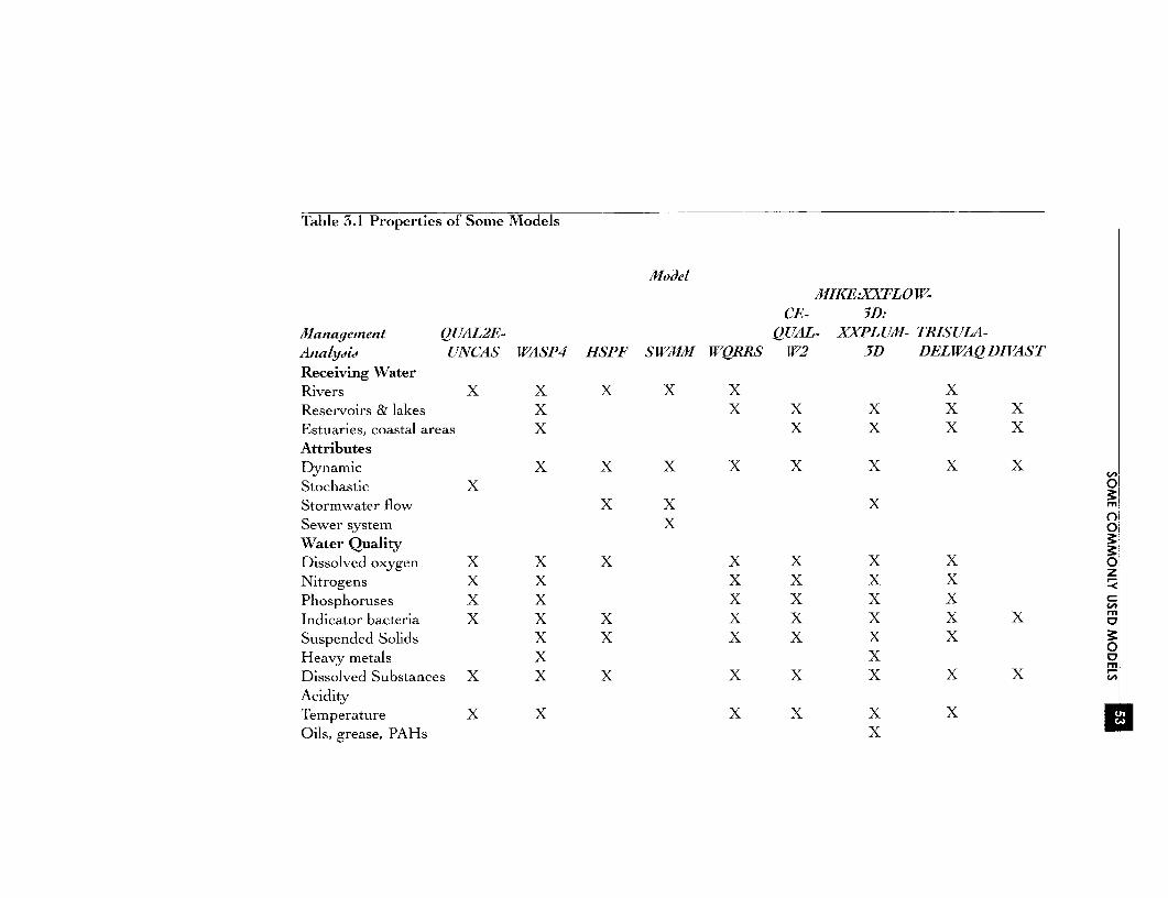
Table 3.1 Properties of Some Models
ModelMIKE.XYFLOW-
CE- 3D:JManagement OUAL2E- QUAL- XXPLUMTI- TRISULA-Analy.sid UNCAS WASP4 HSPF SWMIM WTQRRS W2 3D DELWAODIJVAST
Receiving WaterRivers X X X X X XReservoirs & lakes X X X X X XEstuaries, coastal areas X X X X XAttributesDynamic X X X X X X X X
Stochastic X 0Stormwater flow X X X
Sewer system X 0
Water QualityDissolved oxygen X X X X X X X 0Nitrogens X X X X X X zPhosphoruses X X X X X XIndicator bacteria X X X X X X X X 0Suspended Solids X X X X X X OHeavy metals XDissolved Substances X X X X X X X X
AcidityTemperature X X X X X X
Oils, grease, PAHs X
fl WATER QUALITY MODELING
the effect of the effluent on the receiving water. The diffuser designis important in any outfall (World Health, 1988) and the optionsavailable for the diffuser design are numerous. For example, a well-designed multiport diffuser located in water depths of 50 m can eas-ily achieve initial dilutions of 80:1 and will be equally effective as asecondary treatment for biodegradable components in the waste-water in terms of receiving water concentrations.
Initial dilution is not normally included in the water quality pre-diction models; therefore, the initial dilution for an outfall must bepredicted using models, then the prediction used as an input for thewater quality models. The initial dilution is affected by the jettingvelocity, direction of jets, depth of the diffuser, port diameter, num-ber of ports and port spacing, buoyancy of the effluent, receivingwater velocities (speed and direction), and stratification. Initial dilu-tion is a complex hvdrodynamic process. There are many discussionson the initial dilution hydrodynamics in the technical literature; oneof the most useful is by Muellenhoff et at. (1985).
The U.S. Environmental Protection Agency (USEPA) has devel-oped expert system models for the multiport diffuser outfalls, calledCORMIX (1990 & 1993). These are available at no cost, and theuser manual is particularly good in showing graphically the effects ofthe different variables on the initial dilution. Some model users havefound that the diffuser models overpredict the initial dilution by asignificant amount when the model predictions are compared totracer studies (Sharp & Moore, 1987 & 1989). Users of the diffusermodels may want to reduce the CORMIX model predictions by afactor of two to be conservative, or carry out site-specific tracer stud-ies to quantify the initial dilution predictions of the models. It isadvisable that some site-specific tracer study data be collected forany initial dilution prediction model, because initial dilution is soimportant in determining receiving water quality concentrations. Insome instances, an existing outfall in the area can be used for thetracer studies. The data from the tracer studies can then be com-pared to the model predictions to determine whether a factor shouldbe used for the model predictions. For most outfalls, and particularlyfor the ocean and lake outfalls, the initial dilution varies over a widerange, and it is important that the outfall prediction models be usedto define this range. For some receiving water quality parameterslike CBOD or indicator bacteria, mean dilutions are required,
SOME COMMONLY USED M ODELS
whereas other parameters like ammonia, chlorine, and metalsrequire minimum dilutions. The initial dilution predictions have tobe consistent with the objectives for the water quality parameterbeing modeled.
QUAL2E and QUAL2E-UNCAS (USEPA)
This one-dimensional model, designed for rivers, is a steady-statemodel (assumes instantaneous equilibrium). A good user's manualexplains the theoretical background of the model and provides all theinformation necessary to run the model. The DO and nutrient kinet-ics in the model are complete and have been used directly in othermodels. The UNCAS portion of the model allows uncertainty in theinput data to be incorporated directly in the model predictions. It isone of the few models that includes uncertainty in the water qualitypredictions and has frequently been used to identify the most impor-tant input data for the prediction and the level of precision requiredin these measurements. The model has been used for time-varyingdischarges by carrying out separate runs for a range of dischargeconditions or by incorporating the variability of the discharge as anuncertainty factor in the UNCAS model. The model can be used intwo-dimensional flow situations, but must be applied along thestreamlines. The model temperature prediction is based on heatfluxes and is useful.
The model does not predict heavy metals, oils, grease, or PAHs.While the model can predict indicator bacteria, these predictionsmay not be very accurate if many of the bacterial cells are associatedwith organic flocs. QUAL2 does not have sub-routines for the sus-pended sediment dynamics; consequently, if the suspended solidsconcentrations are high in the receiving water, QUAL2 will have dif-ficulty predicting some water quality parameters.
WASP4 (USEPA)
WASP was designed as a comprehensive receiving water qualitymodel that can be used for all types of receiving waters (rivers,lakes, marine). It is a flexible model that allows users to developtheir own numerical segment system and use various parts of themodel. The hydrodynamics in this model are one-dimensional and
WATER QUALITY MODELING
time-varying; therefore, the direction of the currents must beknown. The model cannot generate a two- or three-dimensionalflow field, and its use is limited if the flow field is characterized bylocalized eddies. In other words, the model will have difficulty whenapplied to a receiving water with unusual topography and bathym-etry, e.g., receiving waters characterized by embayments, offshoreshoals and reefs, breakwaters, or headlands. The user can useanother hydrodynamic model to generate the circulation pattern,then feed the output from this model into the water quality parts ofWAS P.
Predicting the DO, nutrient, sediment, and heavy metal kineticsis one of the great strengths of the model. The receiving waterprocesses in the water quality parameter kinetics have been devel-oped thoroughly in the model. (The model can also be used to pre-dict the receiving water processes for organic substances likepesticides.) The receiving water kinetics is discussed in detail in theuser's manual.
WASP is limited in its hydrodynamic capabilities, the large inputdata requirements to use the model, and the difficulty of quantiflyingthe precision and accuracy of the model, which is a common prob-lem with all complex models. Setting up the model, calibrating themodel, and applying the model require extensive time for technicalstaff.
SWMM (USEPA), HSPF (USEPA, and MIKE 1 (DanishHydraulic Institute)
These models all predict storm wvater runoff and water quality inrivers. Unlike QUAL2, these models are dynamic and predict riverflow. SWMM is a sophisticated model for urban areas with a stormwater sewer system capability. HSPF and MIKE I are similar mod-els for rural areas and do not include sewer networks. For waterquality, the SWMNiM model uses the WASP model for the water qual-ity predictions, while the other models predict water quality usingsimilar equations. These models can include the impact of point dis-charges other than storm wvater. Although the SWMM and HSPFmodels are sophisticated, they can be used as black box models withvery limited input data. This may be a useful feature for predictingstorm water runoff quantity and quality.

SOME COMMONLY USED MODELS U
Except for SWMM, which uses the water quality capabilities ofWASP, the models do not consider the receiving water processes inan integrated manner. The water quality aspects of the models areprimarily transport, dispersion, and first-order kinetics. The modelsare particularly limited in the dynamics of suspended solids in termsof associated bacterial and heavy metal contaminants.
WQRRS (U.S. Army Corps of Engineers)
This is a hybrid model that meshes a river model and a reservoir(lake, estuary) model. WASP has the same capability but is deficientin the reservoir hydrodynamics.
CE-QUAL-W2 (U.S. Army Corps of Engineers)
This is a dynamic, two-dimensional version of QUAL2 specificallyformulated for reservoirs, lakes, or narrow estuaries. The two dimen-sions are downstream and depth. This model considers all the complexprocesses with depth in a deep reservoir that has density stratification.
MIKE XX, TIDEFLOW-3D, XXFLOW-3D, and XXPLUM-3D(Danish Hydraulic Institute)
These models can be dynamically used in one, two, or three dimen-sions or as a Lagrangian spill-type model. The modeling systemdynamically predicts water elevations and currents as well as thesuspended solids dynamics, interactive water quality parametersthat are similar to the processes in WASP. Wave-generatedprocesses are not included explicitly in the model, but their meanimpact can be simulated by adjusting the surface drag coefficients.This is one of the few models that addresses implications of wavedynamics in coastal water quality. These models satisfy all thewater quality and receiving water requirements in this guide. It isnot known whether model precision is available for the modelingsystem, or whether some of the models can be run in a stochasticmanner, other than the XXPLUM-3D models, which are randomwalk models.
Like all complex models, the model setup is labor-intensive, as isthe calibration process, which requires large data sets. Because the
C WATER QUAULITY MODELING
system consists of sub-models for the various components, the indi-
vidual components can be set up and calibrated independently from
the other sub-models. This makes it easier for the user to understand
and calibrate the model.
TRISULA & DELWAQ (Delft Hydraulics)
These models predict the two-dimensional residual (tidal and wind-
averaged) currents and suspended solids dynamics and all the water
quality parameters of interest except for oils, grease, and PAHs as
surface plumes. The water quality processes in the model are simi-
lar in structure to those of WASP, and the sediment dynamics in
DELWAO are more extensive than in WASP. The primary produc-
tivity model predicts diatom and green algal bio-masses. Predicting
and using the residual currents simplifies the calibration process
and is adequate for predicting algal bio-mass but not dissolved oxy-
gen, ammonia, indicator bacteria, and metal concentrations, which
have instantaneous concentration objectives or geometric averages
over a number of samples. It is not known whether the models can
be run in a stochastic manner or whether the models compute the
prediction precision, and it may be necessary for the user to evolve
a method for quantifying prediction precision.
These models can predict all the water quality parameters of
interest except for the oils, greases, and PAHs as surface slicks. The
setup and calibration of complex models require extensive technical
staff time as well as calibration data. Predicting and using the resid-
ual currents simplify the calibration process and are adequate for
predicting algal bio-mass but not dissolved oxygen, ammonia, indi-
cator bacteria, or metal concentrations which have instantaneous
concentration objectives or geometric averages over a number of
samples.
DIVAST (Binnie & Partners)
This model predicts the dynamic two-dimensional currents, water
elevations, and transport of a dissolved substance. The dissolvedsubstance transport process includes first-order time kinetics. Con-
tinuously recorded currents, winds, and water levels can be fed
directly into the model.
SOME COMMONLY USED MODELS
The model does not predict dissolved oxygen, nutrients, sus-pended sediments, heavy metals, temperature, oils and grease, orPAHs.
MODEL DATA REQUIREMENTS AND PREDICTIONISSUES
A list of the site-specific data requirements for all prediction modelsis presented. Because many projects lack some of the data require-ments on the list, water quality prediction models can still be applied.The modeling strategies for limited site-specific data, suspect site-specific data, and non-point source loadings are discussed. The site-specific data required for a model application are discussed. Thenthe use of spill models is discussed.
To develop and use a water resource requires that the develop-ment be carried out in a manner that sustains the water resource fora diversity of water uses. Water resources management requires thedevelopment of water resources projects and/or management proce-dures to preserve and enhance water quality. Water quality predic-tion is the only way that different water resources managementprojects can be evaluated in terms of the water quality aspects; con-sequently, water quality modeling is a fundamental part of allenvironmental assessments.
Water quality models are designed so that they can be customizedto a particular application using some site-specific data. In general,these site-specific data include physical and water quality measure-ments as well as some coefficients and rate constant determinations.Ideally, the user is required to provide site-specific data on the fol-lowing:
1. Physical measurements of bathymetry and topography (flow cross-sec-tions).
2. Boundary conditions (velocity, depth, flow, and concentrations).
3. Initial conditions (depth, velocity, and concentrations).
4. Discharges (location, flow, and concentration).
5. Other coefficients and rate parameters, depending on the water quality
fl WATER QUALITY MODELING
parameter being modeled.
6. Wind and rainfall (some models).
7. One set of measured data for calibration.
8. One set of measured data for verification.
If the site-specific data above are available, the calibrated model
predictions can be expected to have a precision a little larger than the
sum of the precision of the measurements and measurement combi-
nations. The precision of the measurements is defined by the quality
assurance and control program.
In many water resources projects, all the site-specific measure-
ments required are not available and some of the available data maybe questionable. What are the guidelines for using water quality
models in these instances?
Limited Site-Specific Data
When there are limited site-specific data, complete comprehensive
complex models should not in general be used for predictions except
for developing an understanding of the water quality processes in a
particular receiving water or for developing a water quality moni-
toring program. The extensive site-specific data requirements for
comprehensive complex models would render any determination of
the precision of prediction meaningless based on the use of literature
values. Simpler models or simplified comprehensive models should
be used. The following discussion is intended to assist in identifying
the appropriate model simplifications or the preferred model for a
particular application. In this process, the difficulty in measuring
some of the site-specific data discussed previously is considered.
Some site-specific measurements are necessary for any model
application. The basic requirements are 1, 2, and 4 above. Cross-
sectional data are required at the upstream and downstream bound-
ary locations and at a minimum of three locations in between. These
measurements should be for a common flow and/or water depth con-
ditions. If not, these measurements should be adjusted to the same
flow conditions using standard hydraulic techniques. Water depths,
flow, and concentration data must be available at the upstream and
downstream boundaries and at some intermediate cross-sections.

SOME COMMONLY USED MODELS c
Again, these measurements should be for the same conditions of flowand/or water depth as the cross-sectional data and if photosynthesisand respiration are factors at the same time of day.
To determine if photosynthesis and respiration are factors, dis-solved oxygen and temperature (and salinity for marine waters)measurements should be made over a 30-hour period during theaquatic plant growth season. If this is not possible, measure DO andtemperature at several locations early in the morning and at mid-day.If the percentage change in DO percentage saturation in these meas-urements is significant, photosynthesis and respiration are factors inthe DO, and nutrient kinetics in the receiving water must be consid-ered.
The location, flow, and concentrations in the discharges must beknown or estimated. The water quality parameters of interest will beidentified in the preliminary water quality measurements or otherdata. Select the simplest appropriate model from Table 2.2 (remem-ber that dynamic models can be run as steady-state models). lMostmodels have default options and/or provide a range of values for bot-tom roughness, eddy diffusivity, dispersion coefficients, and theother required model coefficients and rate parameters. Because acalibration data set is not available, it is not possible to determine thevalues of the coefficients and rate constants required to apply themodel. These values will have to be selected from values provided inthe manual or some other source. To estimate the impact of thisselection on the predictions, it will be necessary to use the model sev-eral times with different values for the coefficients (sensitivity analy-sis). It is suggested that the model be used with the coefficients/rateparameters in the range of (mean + (0.17 x range)) to quantify theprecision of the predictions. The model in this form may be very use-ful in providing guidance for designing an appropriate monitoringprogram for the model.
If a partial site-specific data set is available, the missing data canbe selected from the range of values in a manner similar to that dis-cussed above.
Another approach is to use a stochastic type model. In thesemodels, the range or mean value and distribution (normal, lognor-mal, etc.) of the user input data can be provided, and the models canbe used stochastically. The predictions from these models willinclude mean value, range, and distribution; consequently, the preci-

WATER QUALITYMODELI NG
sion of the predictions is included in the output. The stochastic form
of the models is the best for limited data sets (Zielinski, 1988).
Suspect Data
In many instances, the data available in a particular project have
been collected at different times, different locations, and by different
agencies using different laboratories. Without some kind of qualitv
assurance and control program in place, it is difficult to assess the
validity of any data. Some simple water qualitv checks can be used
(for example: total organic nitrogen includes ammonia; fecal col-
iforms include F. coi; bacterial density measurement based on a sin-
gle sample is very questionable [coefficient of variation about 0.3
log]; if suspended solids concentrations are high, single samples for
total heavy metal concentrations are questionable; laboratory analy-
sis of dissolved oxygen concentrations, pH, and turbidity are ques-
tionable, etc.) but these are limited. It is important to rememberwhen reviewing data that some or all of the measured data maybe questionable. Equally, the model used for the predictions may
be incomplete and missing some of the important receiving water
processes; consequently, the model can produce erroneous pre-dictions. Similarly, the precision and accuracy of water quality data
must be estimated. Either one can be faultv. If there is a difference
of more than one standard deviation between the measured and the
predicted data, one of the twvo is probably questionable. Identifying
which one is questionable requires checking the predictions of the
model with other measured data sets.
Non-Point (Runoff and Groundwater) Sources
Some of the models in the Appendix predict runoff and groundwa-
ter flows in a sophisticated scientific manner. The export of sus-
pended solids in the runoff is also predicted in the models; however,
the concentrations of water quality contaminants in the runoff and
groundwater are based on statistical results for different types of
land use. It has been shown in numerous studies that about 15 dif-ferent storm events have to be measured before the statisticalrunoff characteristics of a catchment can be defined; therefore,
defining non-point source loadings for a particular catchment can be

SOME COMMONLY USED MODELS
costly. Model users must account for non-point sources in the pre-diction process, but must be aware that estimates of such loadingsmay have a large error (A40 percent for nitrogen, =60 percent forphosphorus and heavy metals). Water quality predictions for periodswhen runoff is not a significant factor will be much more reliable.
Designing a Water Quality Monitoring Program
Once a model has been selected for a particular application, it can beused to determine the most important parameters that should bemeasured to improve the reliability of the prediction. Using the pro-cedures discussed previously for the limited site-specific data, a pre-diction model will have been developed and the precision of themodel predictions will have been defined. The next step is to vary theother input variables like boundary conditions, discharge loadings,cross-sections, etc., and determine the sensitivity of the model pre-dictions to these variations. This process will identify the mostimportant monitoring requirements for the application of the model.As discussed previously, some of the water quality monitoringrequirements are very tedious and costly to carry out, and it isimportant to determine where these measurements are necessary forthe prediction of the water quality. For example: Is it necessary topredict photosynthesis and respiration? Is it necessary to measuresediment oxygen demand and surface re-aeration? Is it necessary tomeasure all the discharges?
QUALITY ASSURANCE AND QUALITY CONTROL
Monitoring Data
Water quality monitoring requires either a field measurement in situ(e.g., temperature, pH, dissolved oxygen, turbidity, depth, velocity)or the collection of water samples that are analyzed in the labora-tory for concentrations of various water quality parameters. Stan-dard laboratory methods have been developed for most waterquality parameters; these are published by various regulating agen-cies. In some instances, field sampling and field handling proce-dures of the samples between the sampling location and the
WATER QUALITY MODELING
laboratory are also specified by some regulating agencies. Theseprocedures reduce variability in the sample collection, transport,and laboratory analysis processes carried out by different personnelin different receiving waters. To quantify the variability associatedwith sample collection, transport and laboratory analysis, most reg-ulating agencies have established quality assurance and quality con-trol (QA/QC) procedures consisting of the following (see forexample USEPA, 1990):
* >10 percent field replicates' and Ž8 replicate samples(for micro-organisms,all samples should consist of at least triplicates;some regulating agenciesspecify the geometric mean of 5 to 10 samples for micro-organisms, inwhich case it may be necessary to collect 5 to 10 replicate samples);
* Ž10 percent laboratory splits* and Ž8 replicate samples;
* Ž5 percent blanks* for both field and laboratory blanks;
* replicate calibration against standards or spikes and/or interlaboratorvsample; and replicate determination of detection levels if not defined inthe standard method procedures.
For conventional water quality parameters, >5 percent has been found ade-quate for field and laboratory spiits and Ž2 percent for blanks.
QA/OC control procedures quantify the precision and accuracyof the water quality data for each measured water quality parameter.Every sampling survey must have quality control data because theprecision and accuracy of the water quality data can be different foreach survey. The detection limit for most water quality parameters isabout 5 times the highest blank concentration; for volatile waterquality parameters, it is about 10 times. Blank concentrations shouldnever be subtracted from measurements. The standard deviation ofthe laboratory splits defines the precision of the analytical technique,and the standard deviation of the field replicates defines the preci-sion of the field sampling, sample handling plus the precision of theanalytical technique. Precision is normally defined as a coefficient ofvariation (%) - (standard deviation x 100)/ mean concentration. Theaccuracy of the analytical method is defined by the calibrationagainst standards and is defined as the standard deviation of at leasteight calibrations. The accuracy of various standard methods is nor-
SOME COMMONLY USED M ODELS i
mally provided in the procedures description. It is acceptable to usethese published accuracy data. For many surveys, quality controldata are also required for positioning, timing, and depth followingthe guidelines for field replicates. A general guide of Ž10 percent forfield replicates should be followed.
The precision and accuracy of water quality data must be quan-tified using quality assurance and quality control procedures. Ifthese data are not available, literature values can be used and the lit-erature referenced.
Model Prediction
Water quality modeling predictions also require quality control, butspecifying quality control procedures for modeling is much morecomplex than for water quality monitoring (Barnwell & Krenkel,1982; Simons, 1985; Benarie, 1987; Ellis et al., 1980; Sharp &Moore, 1987). Both the characteristics of the model and its applica-tion affect the selection of the quality control procedures.
All models have coefficients or rate constants or factors what arerequired for the model to generate predictions-the more complexthe model, the greater the number of the coefficients. Ideally, thecoefficients should be site-specific and determined from local fielddata in the model calibration and verification processes. The inher-ent precision of the water quality data must be considered in the cal-ibration and verification process. In complex numerical models thatare time-variable and in one-, two-, or three-dimensional space, thecoefficients must be defined at each solution point and time step. Thecalibration and verification processes in complex models are labori-ous trial-and-error procedures (Rasmussen & Badr, 1979). Some-times it is possible to simplify the models by carrying out a sensitivityanalysis of the model input requirements to determine the mostimportant parameters in the model. In the sensitivity analysis, themodel input parameters are varied over a small range to determinethe effect of these changes on the predictions. The results of the sen-sitivity analysis can be used to determine the parameter meas-
urement requirements and/or the feasible model simplifications or
may indicate that the selected model is not suitable.If field data are not available, many models provide default
options or typical values that can be used in the models. QA/QC

i WATER QUALITY MODELING
procedures are needed for these coefficients so that the precision inthe predictions associated with the selection of the coefficient valuescan be quantified. Some models can be used stochastically, whichincludes the variability of the coefficients in the prediction (seeDewey, 1984; OUAL2E-UNCAS in Appendix A or OUAL2, 1987;Zielinski, 1988).
Many of the model predictions require the numerical solution ofindividual or coupled partial differential equations normally on aspatially defined grid. It is necessary to select the grid or element sizeand the time step boundary conditions to obtain solutions to theequations. These variables must be selected in such a way that themathematical solutions are stable and converge rapidlv; however, theselection process may affect the precision of the predictions. In gen-eral, longer time steps have less numerical dispersion. The precisionfor these aspects (spatial and time scales) should be quantified in theprocedures.
In many instances, water quality prediction models are used tocompare the effects of different water management scenarios, typi-cally capital works projects. Predictions for these applications arenormally presented as percentage improvement or degradationbetween one scenario and another. While the difference between twomodel predictions is more precise than a single model predictionprocess, there still is a need to quantify the precision of the differ-ences. For example is a 5 or 10 percent difference in the predictionsgreater than the precision for the prediction process?
Defining the precision for the prediction process is also importantin determining the level of the model prediction and the type ofmodel that is the most appropriate for a particular project. For exam-ple, the precision of a three-dimensional model may be too large fora particular application. One way to improve precision is to simplifythe model and/or reduce the number of dimensions to two or one.
Unlike the procedures for water quality monitoring, which can bedefined generically for different water quality parameters, qualitycontrol procedures must be developed for each model application.The objective of quality control in the modeling exercise is to definethe precision of the model predictions for a particular application(Rasmussen and Badr, 1979). Ideally, the precision should be evalu-ated for the model components like hydrodynamics, mass balance,receiving water process, and sediment dynamics, separately if possi-
SOME COMMONLY USED MODELS D
ble, because the magnitude of the precision can be different for eachof the components. This information is useful in providing directionfor future monitoring and modeling efforts. If one of the modelingcomponents has a precision much greater in magnitude than the othercomponents, the precision in this component can be improved byincreasing the monitoring effort for this component or by simplifyingthe model. In evaluating the component precision, it is necessary toaccount for the dependence of one model component on another com-ponent; e.g., the mass balance component uses the output from thehydrodynamic component and, consequently, includes the precisionfor this component. For the selection of the appropriate model and thelevel to be used in that model, the following procedure could be used:
* List the available site-specific data.
* Summarize the historical information on water quality problems ordegradations. This information should include both water qualitymeasurements (quantitative) and qualitative data.
* Visit the site to confirm historical information on water quality and tonote any special factors in the receiving water that relate to water qual-itv modeling. These factors could include observations of visible sur-face slicks, receiving water color or turbidity, aquatic plant growths,backwater areas, recreational swimming or fishing, visible bottom sed-iments, private domestic sewage discharges, irrigation withdrawals,livestock watering or crossing, etc.
* Interpret the available site-specific data, historical information, and sitevisit information.
* Quantify the precision and accuracy of the available data. If qualitycontrol data are not available, use literature values for the method usedto measure the data. If only laboratory analysis precisions are available,use 1.2 X (laboratory precisions) for the precision for field plus labo-ratory analysis.
* Select water quality models that are suitable for the project (i.e., mod-els that satisfy the water quality prediction objectives).
* List the input requirements for each model candidate.
* List the model input requirements for which there are no site-specificdata available. Based on the interpretation of the available data, histor-
nfWATER QUALITY MODELING
ical information, site visit, and list of the required model inputs that are
not available locally, simplify the candidate models and then select the
most appropriate model(s). A site visit is extremely important in the
model selection process.
* Set up the necessary topographical grids for the selected model(s).
* For the missing input requirements for the selected model(s), deter-
mine a range for each input using published values or values from
related projects. Determine the range of values for the available site-
specific data. Now predict the water quality concentration with the
model (CA) using one-third of the range for all input parameters. Then
predict the water quality concentration with the model (CB) using two-
thirds of the range for all input parameters. An estimate of the model
precision expressed as a percentage = (CA+CB)/((CA+CB)/ 2 ). Alterna-
tively, it can be assumed that the coefficient of variation is on the aver-
age 15 percent for all input requirements. If six to eight separate model
predictions are made randomly selecting values within ± coefficient of
variation, the standard deviation of the predictions is a good estimate
of the model precision (Dewey, 1984).
• If the model precision is within 50 percent of the site-specific measured
data, the selected model probably has the appropriate sensitivity for
project use.
Other more rigorous methods to determine the model predictionprecision are preferred for any particular model and its application.
A method can be used at the discretion of the model user. For the
non-linear numerical models, some method based on chaos or sensi-
tivity analyses may be appropriate. It is not possible to quantify the
precision of a model prediction with a single prediction verification
for deterministic or numerical models. One of the best methods for
quantifying precision is to use the stochastic or Monte Carlo formu-
lation of the model(s). In some instances, it may be appropriate touse a stochastic model as an additional instrument to provide an
estimate of the precision if stochastic forms of the models are not
available.Any selected model may not include some of the important
processes in the receiving water; therefore, the prediction will be
imprecise. For example, a model may not include the impact of the
resuspension of bottom sediments on water quality, and this may be

SOME COMMONLY USED MODELS
Typical Sensitivities for Specific Water Quality Parameters
Temperature 2-3%BOD 10-20%Dissolved oxygen 5-10%Nitrogen 15-30%Phosphorus 15-40%Algal 10-25%Bacteria 0.2-0.35 logConservative 5-10%Heavy metals 25 50%Cohesive sediments and flows 50-100%
the major loading source in some receiving waters. Or a model maynot include atmospheric loadings. These model formulation discrep-ancies will probably not become apparent until the model predic-tions are shown to be consistently different from measurements. Thisis one of the reasons that multiple verifications are required to besure that the model selected contains all the most important vari-ables.
In some instances, the precision of the prediction for the waterquality parameter of interest may be very large (for example, withinone order of magnitude) and therefore not very useful for waterquality management; e.g., indicator bacteria, phosphorus, heavymetals. In these instances, the model user can carry out numerouspredictions to statistically improve the precision, or simplify themodel, or use a surrogate parameter. The surrogate can be used forpredicting transport, dispersion, and settling. Then, the surrogateconcentrations can be related to the concentrations of the parameterof interest through studies. Or the surrogate can be used to predictthe transport, dispersion, and settling to which have been added theother processes relative to the water quality parameter of interest,like mortality rate for indicator bacteria. Suspended solids concen-trations have been used extensively as a surrogate parameter forstorm water quality. In sanitary wastewaters, suspended solids con-centrations are about 200 mg/L. Dissolved solids concentrations as

WATER QUALITY MODELING
measured by specific conductivity have also been used as a surrogateparameter for wastewaters. The conductivity of sanitary waste-waters is over 1,000 umhos/cm.
The precision and accuracy of water quality data must be quan-tified using generally accepted quality assurance and quality controlprocedures for water quality modeling. The precision and accuracyfor the model predictions must be developed for each model applica-tion. Stochastic forms of the prediction models are useful in quanti-fying the model prediction precision and accuracy.
Spill Models
Spill models were discussed previously. Normally, these models canbe used with little site-specific data; however, the same Lagrangianspill models can also be used to predict a plume, which can be onthe water surface or at depth. In the Manila Second Sewerage Pro-ject, for example, site-specific data were used to generate the cur-rents at the ocean disposal site, as well as backgroundmeasurements of the ocean concentrations in the vicinity of the pro-posed dumping sites. The resulting ocean plumes were predicted fordifferent conditions and different locations so that the optimum dis-posal site could be selected. The spill models are required for short-period discharges or releases of substances that can degrade thereceiving water quality. In this instance, a quantity of tracer dye isinstantaneously released, and the tracer concentrations are meas-ured in the tracer plume at various times thereafter. Using a spill-type model, the dispersion coefficients can be determined from thetracer plume measurements.

! ~C H A PT E R 4
Case Studies of ModelsApplied to World Bank
PoectsProysst
This chapter presents seven diverse case studies from China,T India, and the Philippines. The case studies were taken fromprojects implemented with funding by the World Bank. In
each case, the modeling work was necessary in order to allocatescarce financial resources so as to maximize environmental benefits.
DETAILED HYDRODYNAMIC AND WATER QUALITYMODELING STUDY, 1998, CHONGQING, CHINA
The municipality of Chongqing has a population of about 30 millionin an area of 82,000 km2 along the Yangtze River and Chang JialingRiver (the third longest river in the world, with a mean annual flowat Chongqing of about 100,000 m3/s) upstream from the ThreeGorges Dam. The City of Chongqing is located at the confluence ofthe Yangtze and its major tributary the Jialing.
Water supplies for the City of Chongqing are derived primarilyfrom the Jialing and, to a lesser degree, from the Yangtze. Theserivers also receive discharges, largely untreated, of municipal andindustrial wastewater from the city. These discharges are poorly dis-persed in the river water, and some are upstream from water supplyintakes. Thus, despite the very large flow and assimilative capacityof the rivers, the quality of raw water supply, particularly from theJialing, is often poor.
The construction of the Three Gorges Dam will increase thewater depth of the Yangtze by up to 16m and significantly reduce thevelocity of the river to less than low-flow conditions. Major invest-ments were therefore required for wastewater management infra-structure in the City of Chongqing. The magnitude of the associated
71
i WATER QUALITY MODELING
costs necessitated a phased approach to the provision of sewerage
system improvements and wastewater treatment plants.
Secondary treatment of all wastewater would meet water qual-
ity objectives but at a high cost, in part because of the high cost of
land in the urban area. The water quality problems of the Jialing
could, however, be readily and economically solved by improved
collection of wastewater and discharge into the Yangtze down-
stream of the confluence. This would effect substantial environ-
mental improvement within the urban area of Chongqing at a cost
significantly lower than that of full treatment of all wastewater dis-
charges.
The Yangtze, however, provides water supplies for a large popu-
lation in its catchment downstream of the Jialing confluence, includ-
ing the important cities of Fuling and Wanzhou. It was therefore
necessary to determine how such an option would affect water qual-
ity in the Yangtze in the immediate term and, if determined to be
beneficial, the time scale within which wastewater treatment wouldneed to be introduced.
Summary of the Project
These issues were investigated by means of mathematical water
quality modeling for the Yangtze and Jialing, with two objectives:
1. to evaluate the effects of wastewater discharge (at various levels of
treatment) from Chongqing on water quality in the Yangtze in a far-
field context to determine the level of compliance with water quality
objectives for the Yangtze and the need for wastewater treatment;
and
2. to use near-field modeling of the effects of wastewater discharges in the
Yangtze to optimize the discharge arrangements so as to minimize the
negative effects on water quality by efficient mixing.
The modeling was undertaken by Chongqing EnvironmentalProtection Bureau and the Danish Hydraulic Institute (DHI),
with financial assistance from the Government of Denmark. The
DHI MIKE system of models was used in the one-dimensional
form for the far-field and two-dimensional form for the near-field
modeling.
CASE STUDIES OF MODELS APPLIED TO WORLD BANK PROJECTS
The one-dimensional model MIKE 11 was set up for the Yangtzeand Jialing Rivers. In this application, MIKE 11 consisted of fourcomponents: NAM (a precipitation runoff model), HD (a hydrody-namic model), AD (an advection and dispersion model), and WO (awater quality model). The governing equations in each model arepresented in this guide. These equations are a set of partial differen-tial equations which are numerically solved at all the grid points in atopographical network established to represent the river using atime- and space-centered finite difference scheme to minimize thenumerical dispersion in the solution. The spatial and time steps usedin the solution are selected to ensure that the solution is stable andrapidly converges. The required inputs for each model are presentedin the report.
The models were then calibrated on the basis of data available for1986-87 and verified if possible against the 1993-94 data. Calibrationis the process of adjusting coefficients, initial conditions, and bound-ary conditions so that the predictions match the calibration data set.For the hydrodynamic model including NAM measured and pre-dicted water levels, river flows and accumulated flows werematched. The calibrated parameters are presented in tables, and thecalibrations shown graphically in this guide. The AD componentwas calibrated by adjusting dispersion coefficients and initial andboundary conditions for dissolved substances. The calibrationprocess for dynamic finite difference schemes is a laborious trial-and-error process.
The processes in the water quality component of the model fordissolved oxygen include biochemical oxygen demand loadings;rates of BOD degradation, re-aeration, photosynthesis, and sedi-ment oxygen demand; nitrogen loadings; rates of nitrification, den-itrification, sedimentation, and resuspension; and the uptake byalgae and plants. The water quality model predicts temperature andconcentrations of DO, BOD, ammonia- N, nitrate-N, phosphorus(as P), and fecal coliform. The most important calibrated parame-ters are presented in tables, and the calibrations presented graphi-cally (Figure 4. 1). Establishing the point and non-point dischargesto use in the model was not a simple task, because flow and con-centration data were not available for all discharges to the river.Figure 4.2 shows the discharges used for the modeling for the Jial-ing River.

WATER QUALITY MODELING
Figure -. 1 Simulated Concentrations Along Jialing River 1987
IDissolved oxgen
10
15 Mari E14 I Aug
2 1~~~~~~~~~~~~~~ Novi2
350 450 550 650 750 850 950 1050km
2
Ammonia_ ~~~~~~~~~~~~~~15 Mar
1 AugI Nov
350 450 550 650 750 850 950 1050km
The calibrated model was then verifed using the 1993-94 data
set. It was found that the simulated water levels and measured level
were in good agreement during the dry season. There were some dif-
ferences at some locations during the wet season. However, because
the accumulated flows during the dry season were within 5 percent
of the measured data, the calibrated model was considered appro-
priate for evaluating the water resources alternatives. There were
more differences between the simulated and measured water levels,with the simulated as much as 1.5 m below measured. The difference
in water levels and river cross-sections was considered to be insignif-
icant because the simulated water levels were less than those meas-
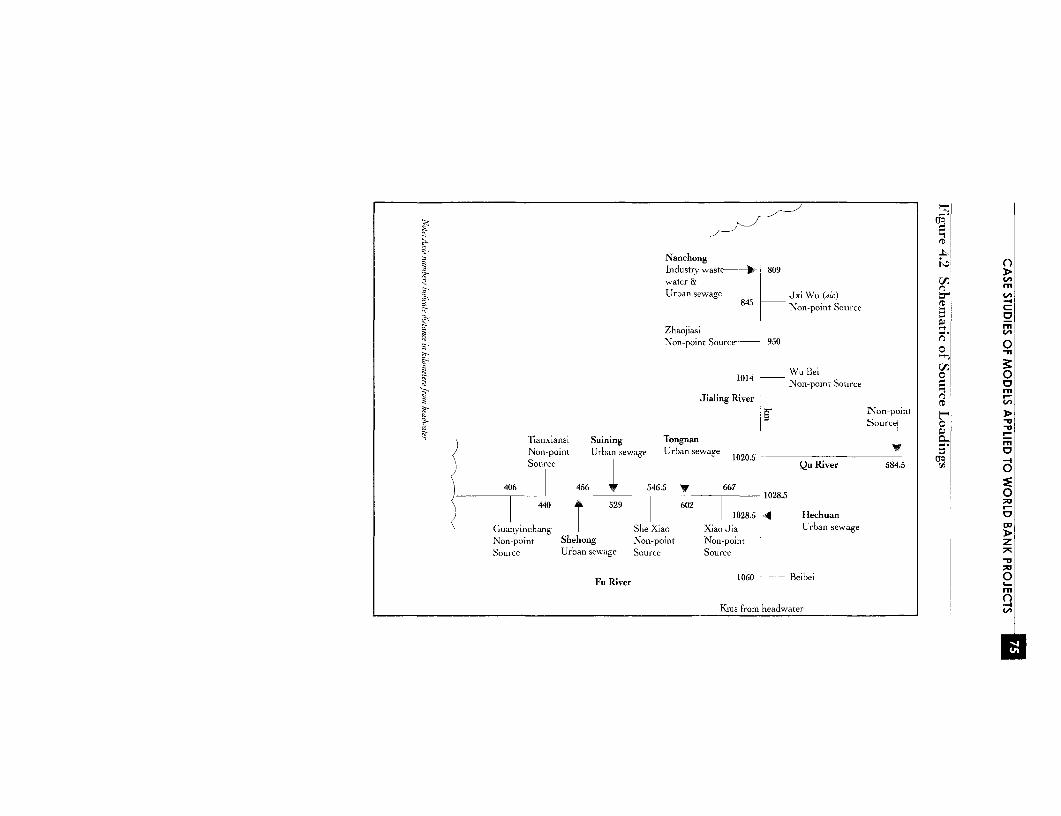
NanchongIndustry waste-)- 809 >water CA
Urban sewage Jxi Wu (dic) CA845 -Non-point Source CD
Zhaojiasi vi
Non-point Source 950 O0 -n
104 Wu Bei Sorc- 1014 ~~~~~~~~~~~~~~~ ~ ~ ~ ~ ~~Non-point Source 16
Jialing River m-
t r ~~~~~~~~~~~ ~ ~~~~~~~~~Non-point r:Source 0
Tianxiansi Suining Tongnan r n mNon-point Urban sewage Urban sewage 1020.
Source Qu River 58-1.5 t O
406 456 V 546.5 V 667 1028.5 0440 529 602
1028.5 4 Hechuan
Guan6inchang She Xiao Xiao Jia Urban sewageNon-point Shehong Non-point Non-point Z
Source Urban sewage Source Source
Fu River 1060 Beibei 0
Kmns from headwater
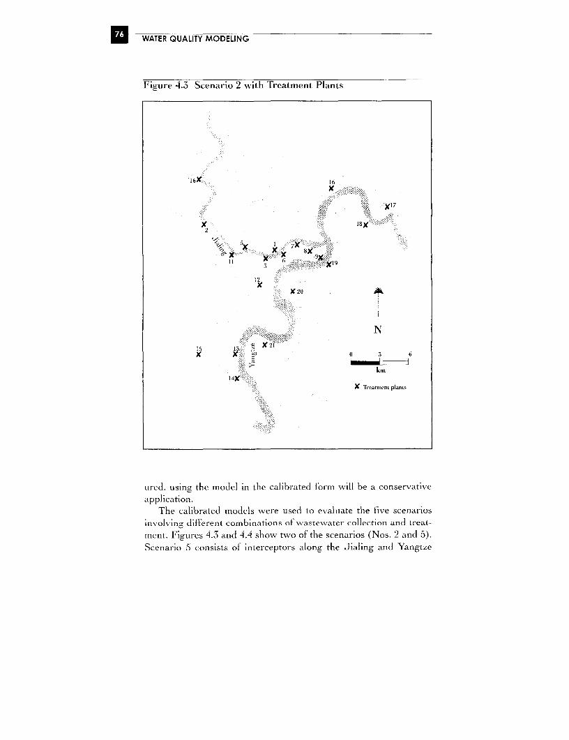
U WATER QUALITY MODELING
Figure .3 Scenario 2 with Treatment Plants
ieiK 16
2
K 8KK 1 7K
3 K1~~~~~~9
12
DX2
N
15 13 X K21K K ' 3 6
km
X Treatment plants
ured, using the model in the calibrated form will be a conservative
application.
The calibrated models were used to evaluate the five scenarios
involving different combinations of wastewater collection and treat-
ment. Figures 4.3 and 4.4 show two of the scenarios (Nos. 2 and 5).
Scenario 5 consists of interceptors along the Jialing and Yangtze
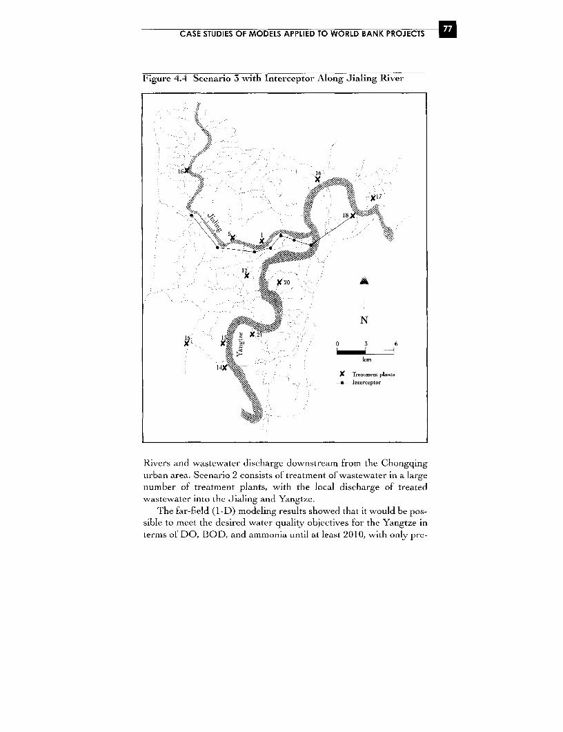
CASE STUDIES OF MODELS APPLIED TO WORLD BANK PROJECTS U
Figure A. Scenario 3 with Interceptor Along Jialing River
16* 16
P'' 4
i /Ri :~ ~ ~~ X jx1
.- i'~~~~~~~~~~~~~i
12
'-2'"A0 A
;2l .'4 N
15 I~1 X5.' K , t) , , 0 3 6
km
X Treatment plants-a-- Interceptor
Rivers and wastewater discharge downstream from the Chongqingurban area. Scenario 2 consists of treatment of wastewater in a largenumber of treatment plants, with the local discharge of treatedwastewater into the Jialing and Yangtze.
The far-field (1-D) modeling results showed that it would be pos-sible to meet the desired water quality objectives for the Yangtze interms of DO, BOD, and ammonia until at least 2010, with only pre-

fl WATER QUALITY PAODELING
liminary treatment of Chongqing wastewater discharged to theYangtze downstream from the confluence with the Jialing. Subse-quently, wastewater treatment would need to be introduced, in par-ticular to control nutrient loads.
The modeling enabled development of a phased program ofwastewater infrastructure for the city based initially on wastewaterinterception and conveyance by a system of major tunnels for dis-charge to the Yangtze. An overall treatment strategy was developedfor Chongqing to sustain and protect water quality in the Yangtzeand to prepare for the probable requirements for control of nutrientloads to the Yangtze in the light of possible eutrophication of theThree Gorges Reservoir.
The local water quality in the river reaches through theChongqing area was evaluated with a two-dimensional model,MIKE 21. MIKE 21 is similar in structure to MIKE 11, with HD,AD, and WQ components. The equations used in the model are pre-sented in this guide. The model was run for five-day periods and wascalibrated using 1987 data and verified using 1994 data. The veloc-ity vectors in the river were simulated. Figure 4.5 shows the simu-lated maximum ammonia concentrations.
The 2-D near-field modeling identified the optimum dischargelocation and diffuser configuration for the discharge of the waste-water into the Yangtze to minimize the mixing zone required. It par-ticularly highlighted the importance of discharge via a diffusersystem into the deep river channel.
Costs
The project costs were about US$400 million. Modeling costs ofUS$500,000 were provided by the governments of Chongqing andDenmark. This is equivalent to only 0.1 percent of the overall proj-ect cost, but importantly, the modeling confirmed the applicability ofthe proposed phased program, resulting in savings on the order ofhundreds of millions of dollars.
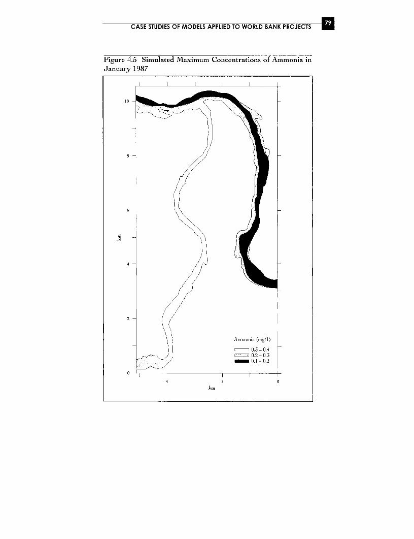
CASE STUDIES OF MODELS APPLIED TO WORLD BANK PROJECTS U
Figure 4i.5 Simulated Maximum Concentrations of Ammonia inJanuary 1987
10
8
6
4
2
Ammonia (mg/I)
0.3 -0.40.2 -0.30.1 -00.2
O4 2 0
km

A WATER QUALITY MODELING
OCEANOGRAPHIC AND WATER QUALITYMODELING STUDIES AT MUMBAI, INDIA, 1997
The island city of Mumbai, India, generates about 2 million Mm 3 /d
of sewage, most of which is discharged untreated into the Arabian
Sea. As part of the Bombay Sewage Disposal Project, design and
environmental assessment (EA), some limited modeling work was
carried out during 1990-95 to assess the proposed project's effects
on the water quality of the coastal areas and tidal creeks. The EA
recommended more extensive studies, including development of
mathematical simulation models to evaluate treatment and outfall
options for the next stage of sewerage investments in Mumbai.
Based on these recommendations, a comprehensive coastal water
quality study was commissioned in 1995. It developed an integrated
hydrodynamic and water quality model to simulate fecal coliform
densities for 35 km of shoreline and extending offshore for 15 km;
to collect bathymetry, tidal, and current data appropriate to cali-brate the prediction models for both monsoon and non-monsoon
periods; and to carry out tracer and indicator bacterial decay meas-
urements.
Water Quality Modeling Requirements
The requirements were, using collected physical and water quality
data in the area of concern, to develop and calibrate a water quality
model suitable for assessing the effects of different levels of treat-
ment and different outfall lengths and locations on the coastal water
quality. The assessment process was required to identify the most
cost-effective pollution abatement option for enhancing the coastal
water quality.
Summary of the Project
Binnie and Partners, Ltd., of the UK had carried out the original
limited assessment studies, and the National Environmental Engi-
neering Research Institute (NEERI) of India was contracted by the
Municipal Corporation of Greater Mumbai to carry out the detailed
water quality modeling, using Binnie and Partners' model, DIVAST
(Depth Integrated Velocity And Solute Transport), through a sub-
CASE STUDIES OF MODELS APPLIED TO WORLD BANK PROJECTS
contract. This is a dynamic two-dimensional finite difference modelwhich assumes that the circulation in the area of interest is prima-rily horizontal (parallel to the water surface) and not stratified withdepth. A basic grid size of about 200m by 200 m was used for themodeling area, which extended 35 km along the shore and 14-17 kmoffshore but varied in some areas to reduce the computational timein the model. Typically, the numerical model was run for 48 hoursof real time. Data from recording tide gages (3 in the model area)and recording current meters (10 in the model area), as well asmeasured bathymetry and topography, were used as inputs to themodel (see Figure 4.6). The open model boundary to the north usedrecorded water levels, and the open boundary to the south recordedcurrents. Wind data were available from two shore-based locations.
The bottom roughness coefficients, surface wind drag coeffi-cients, eddy coefficients, and model time steps were adjusted tomatch simulated and measured currents and water levels in themodel area (see Figure 4.7). To calibrate the solute model compo-nents, tracer plume data were available for rising and falling tides at
three locations using Rhodamine B and at one location using theradioisotope 8 5 Br (half-life 36 hours) in an ammonia bromide solu-
tion. The decay rates for the indicator bacteria were measured in thelaboratory twice for simulated receiving water conditions. The solute
coefficients, like dispersion coefficients, were adjusted in the calibra-tion process so that the model-simulated predictions corresponded tothe measurements. Once the models were calibrated, they were used
to simulate monsoon and non-monsoon conditions (see Figure 4.8).
The model was used to assess the impact of primary and second-
ary treated effluent discharged at various distances offshore (3-88km) for the spring and neap tidal conditions and both the maximumand minimum initial dilution conditions at the outfall. Figure 4.9shows the variation of fecal coliform densities for the primary treat-
ment scenario.
The model simulations showed that the wastewater plumes were
greatest in extent during the non-monsoon periods. At two loca-
tions, extending the outfalls farther offshore did not significantly
reduce the size of the effluent plumes owing to local circulation pat-
terns. The simulations also showed that secondary treatment would
not significantly improve the nearshore water quality at Worli andBandara.

* WATER QUALITY MODELING
Figure -i.6 Current Meter and Tide Gauge Locations and Model
Area
Vasai Creek
1039
X5
4 3 12 ~~~~~~~~~~~~ThaneCreek
t T ~~~Butcher X
= = X *M 1aLb arg Island
ColabaPoint ?oe
LEGEND
X Current Meters
) Tide Gauges
NVastewater Outfalls
a mLandO 5KS IOKM 201 M
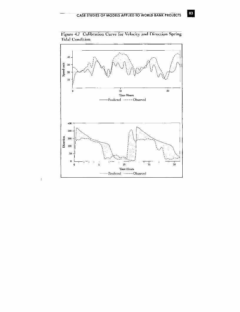
CASE STUDIES OF MODELS APPLIED TO WORLD BANK PROJECTS U
Figure 4.7 Calibration Curve for Velocity and Direction SpringTidal Condition
40-
20 20
10 A
0 10 20
Time Hours
-Predicted ----- Observed
400-
300
e *~200 - ---
50 -I
00 5 10 15 20
Time Hours
-Predicted ----- Observed

g WATER QUALITY MtODELING
Figure -. 8 Fecal Coliform Densities at 3 and 8 Km for PrimaryTreatment
Tides
('
N
0
km
Land
Costs
For 1996, the estimated costs for Worli were US$60 million for pri-marx' treatment and US$212 million for secondary treatment; atBandara, the costs wereUS$97 million and US$286 million,respectively. The outfall costs wereUS$8.7 million per 500 meters.The complete coastal water quality modeling studies cost wereabout US$880,000. Financing came from a PHRD (Japan) grantadministered and managed by the World Bank, with contributionsfrom the City of Mumbai and from NEERI, the study consultants.
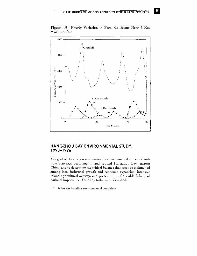
CASE STUDIES OF MODELS APPLIED TO WORLD BANK PROJECTS
Figure -. 9 Hourly Variation in Fecal Coliforms Near 3 KmWVorli Outfall
5000
~4000 1 ;ufI
g3000m /
2000 -
1 Km South
1000 A/x\\ $/ X I Km North X X
O 6/ /~v $s ."\
0 10 20 25
T`me Hours
HANGZHOU BAY ENVIRONMENTAL STUDY,1993-1996
The goal of the study was to assess the environmental impact of mul-
tiple activities occurring in and around Hangzhou Bay, eastern
China, and to determine the critical balance that must be maintained
among local industrial growth and economic expansion, intensive
inland agricultural activity, and preservation of a viable fishery ofnational importance. Four key tasks were identified:
1. Define the baseline environmental conditions.
D WATER QUALITY MODELING
2. Estimate the environmental impact of ongoing development around the
bay.
3. Develop strategic plans and policy statements.
4. Consider the planning options over a 2 0-year period.
Water quality models were extensively used to assess the various
non-intervention and intervention options.
Water Quality Modeling Requirements
A hydrodynamic numerical model was required to simulate the cir-culation patterns in the bay for different tidal conditions, river
flows, and wind climates. Superimposed on the hydrodynamicmodel, a water quality model was required to predict sedimenttransport/deposition/resuspension, nutrient and phytoplanktondynamics, dissolved oxygen/biological oxygen demand kinetics, andheavy metal dynamics. The calibrated hydrodynamic and waterquality models were then used to assess the merits of various inter-vention options.
Summary of the Project
The modeling was carried out by Delft Hydraulics and Mott Mac-Donald international consultants, using Delft's TRISULA hydrody-namic model, a two-dimensional finite element model using acurvilinear grid (see Figure 4. 10). The tidal flow was calibrated first,followed by a salinity calibration. The methods for generating modelinput data at the open sea boundaries of the model to the east andsouth (no site-specific data were available), determining the best val-ues of bottom roughness (no site-specific data were available), anddetermining the best eddy viscosities are discussed in this guide.Open boundary data and bottom roughnesses were adjusted tomatch measured water level data, and the eddy viscosities wereadjusted to match measured salinity data. Adjustments were alsomade to achieve the appropriate residual flow in the model. Anexample of the circulation field predicted by the hydrodynamicmodel is presented in Figure 4.11.

CASE STUDIES OF MODELS APPLIED TO WORLD BANK PROJECT SE
Figure 4i.10 Nested Finite Element Grid
_~~~~~~~~~~~~~~Fn Grid_
t1IxLand
Delft used its water quality model called DELWAO, which usedthe circulation pattern simulated by the hydrodynamic model asinput. DELWAQ predicts cohesive suspended solid kinetics (sedi-mentation, resuspension, absorption, and mitneralization), nutrientdynamics including nitrification and denitrification, dissolved oxy-gen processes, phytoplankton kinetics, heavy metals, and indicatorbacteria. The water quality calibration process was similar to thehydrodynamic calibration and was carried out sequentially as fol-lows: transport of suspended par-ticles followed by total concentra-tion levels, then water quality and ecological processes. Some of themodel parameters adjusted in the calibration process included criti-cal shear stresses; settling velocities; dissolved and detritus compo-nents of nitrate, ammonia, phosphate, and silicon; phytoplankton
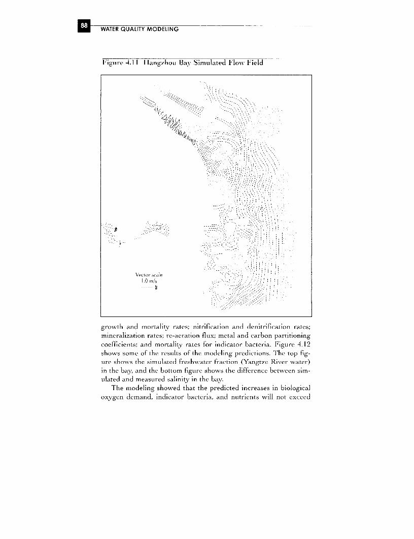
g WATER QUALITY MODELING
Figure .11 Hangzhou Bav Simulated Flow%- Field
Vector scale1.0 M/s"
growth and mortality rates; nitrification and denitrification rates;
mineralization rates; re-aeration flux; metal and carbon partitioning
coefficients; and mortality rates for indicator bacteria. Figure 4.12
shows some of the results of the modeling predictions. The top fig-
ure shows the simulated freshwater fraction (Yangtze River water)
in the bay, and the bottom figure shows the difference between sim-
ulated and measured salinity in the bay.
The modeling showed that the predicted increases in biological
oxygen demand, indicator bacteria, and nutrients will not exceed
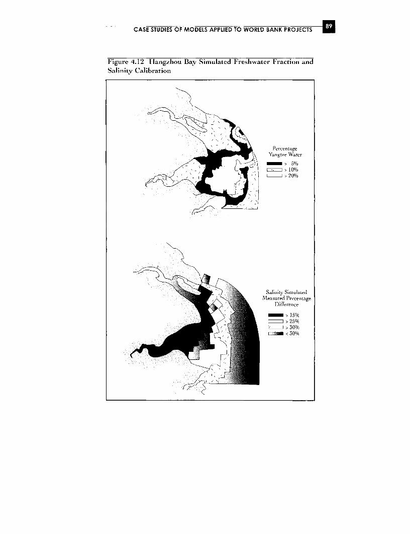
CASE STUDIES OF MODELS APPLIED TO WORLD BANK PROJECTS
Figure 4.12 Hangzhou Bay Simulated Freshwater Fraction andSalinity Calibration
PercentageYangtze Water
> 10%9 g v~~~~~~~~~~~~ t20%
Salinity SimulatedM easured Percentage
Difference
> 15%>25%
>~ 30%<30%
g WATER QUALITY MODELING
the assimilative capacity of the bay. However, because primary pro-ductivity is presently limited by high concentrations of suspendedsolids in the bay, any reduction in suspended solids concentrationswill result in higher phytoplankton bio-masses, which could lead togreater occurrences of undesirable algal blooms because of theabundance of nitrogen available. Rural nutrient controls must beimplemented in the river catchments if these blooms are to be con-trolled. The increased loadings of copper and zinc will result inincreased sediment concentrations offshore on the order of 50 per-cent, which will have a accumulative effect on benthic organisms.Metal discharges in the river catchment areas need to be controlled.
Costs
Half a million tonnes of fish are annually harvested in the bay (10percent of China's total production), and an evolving tourist indus-try on the islands is dependent on the water quality in the bay. Thecurrent annual commercial value of these resources is large. Thewater quality modeling cost relative to the annual commercial valueof the resource was less than 1 percent.
SECOND SHANGHAI SEWERAGE PROJECT (SSPII),1996
This project was the second stage in a comprehensive program forprovision of wastewater management facilities for the city of Shang-hai, China. The first stage had diverted 1.4 Mm3/d of wastewaterfrom the catchment of the Suzhou Creek in urban Shanghai for dis-posal to the Yangtze Estuary after preliminary treatment at a sub-marine outfall at Zhuyuan. The SSPII provides for the disposal ofadditional wastewater from the urban area, initially a discharge of1.7 Mm3/d, and ultimately 5 Mm3 /d, to the Yangtze Estuary at Bai-longgong
The objectives of the project were to enhance wastewater andstormwater management by expanding wastewater collection, pre-treatment, and disposal capacity and stormwater drainage facilities;to reduce urban pollution; to improve wastewater utility financialand operational management; and to strengthen sector institutionsthrough training.
CASE STUDIES OF MODELS APPLIED TO WORLD BANK PROJECTS U
An environmental assessment was required to determine the pos-sible effects on the local water quality in the Huangpu River andYangtze Estuary.The environmental assessment confirmed that theassimilative capacity of the Yangtze River (mean annual flow 30,000m3/s) was such that in a far-field context, the discharge of theplanned quantities of wastewater would not significantly adverselyaffect water quality in the immediate term. However, water qualitymodeling was necessary initially to assist in determining the optimallocation of the outfall discharge at Bailonggong and the optimal dif-fuser configuration in order to minimize the near-field impact of thewastewater discharge.
The success of this project was ensured by the positive and coop-erative working relationship between the Government of Shanghaiand the technical staff from the East China Normal University andthe Danish Hydraulic Institute.
Summary of the Project
Water quality modeling was required to determine the optimal out-fall location, its design, and the wastewater treatment strategies,including the concept of phasing the project. In particular, waterquality modeling was required to assess the nutrient loadings to theestuary and their implications in the frequency of occurrences of redtides in the estuary. The initial capacity of the outfall was 1.7Mm3/day, with an ultimate capacity of 5.0 Mm3/day.
The water quality modeling was undertaken by the governmentof Shanghai, which engaged local Shanghai specialists from the EastChina Normal University and arranged for additional support fromthe Danish Hydraulic Institute. It was recognized at the outset thatthe circulation characteristics in the Yangtze Estuary are a complexfunction of the river flow, tidal stages, wind climates, and the JapanCurrent (Kuro Shio); consequently, the currents in the estuary varyin both time and three-dimensional space.
The DHI MIKE system of models was used for the predictions(for details, see Appendix) These models numerically solve theappropriate coupled partial differential equations on a rectangulargrid. Three nested hydrodynamic models were used in this project,with grid sizes of l,OOOm (MI), 250m (M2, and 40m (M3). Thelarger-scale models (MI and M2) were two-dimensional, and the

E WATER QUALITY MODELING
smaller scale three-dimensional. The areas modeled are shown inFigure 4.13. The results from the MI model were used as boundaryconditions for the M2 model, and the M2 results for the M3 model.The model inputs included bathymetry, bottom roughness, eddycoefficients (no site-specific data were available), tidal conditions,wind climates (shore-based measurements), and river flows. First,the MI1 model was calibrated by comparison between the predictedwater levels and the measured values for tidal water level variationsand wind and net flow conditions. A similar calibration process wascarried out for the M2 and M3 models. In addition, the calibrationof M2 model included the comparison between the simulated andmeasured current velocities.
The water quality process for quantifying the required modelinput parameters like dispersion, biological oxygen demand, indica-tor bacteria decay coefficients, and suspended solids partitioning
Figure -. i5 The Alodel Domain
A12
N
Eastern
._~~~~~~~~~hn Se
CASE STUDIES OF MODELS APPLIED TO WORLD BANK PROJECTS i
coefficients for the heavy metals is discussed. The iM2 water qualitymodel was calibrated for indicator bacteria, biological oxygendemand, dissolved oxygen, ammonia, nitrate, and phosphate over a7.5-day period for both a dry season (March) and a wet season(July). In the calibration process, the decay rate and temperaturecoefficients, nitrification and denitrification constants, nutrient con-tents of organic matter, and suspended solids partitioning coeffi-cients for metals as well as the sedimentation and criticalresuspension velocities were adjusted to produce predictions thatwere similar to the measured values.
The models were used to assess different abatement options, withemphasis on comparing modeling predictions for different optionsrather than comparing the model predictions with water qualityobjectives or standards (see Figure 4.14). The model predictionsshowed that the assimilative capacity of the Yangtze River Estuaryis mainly dependent on the river discharge, tidal variation, back-ground concentration, and biochemical processes in the estuary. Thegoal of the outfall design and location study was to optimize exploita-tion of this assimilative capacity, which is a direct function of thewater quality standards for the estuary. The simulated results con-firmed that 1.7 Mm3/day of wastewater could be discharged at Bai-longgong without significant adverse effect on the water quality ineither the near or far field. The optimum diffuser configuration, rec-ommended in light of the modeling results, ensured complete mixingwithin a limited area in the near field and comprised a 20 0m-longmultiport diffuser consisting of six risers. For aesthetic purposes, itwas recommended that oils be reduced in the effluent.
The water quality modeling was also used in the development ofa longer-term strategy for wastewater treatment for Shanghai, inparticular the need to control nutrient loadings to the Yangtze Estu-ary. This was important because nutrient loads affect the frequencyof red tides in the nearby Hangzhou Bay.
Costs
The capital costs for the overall project were estimated to be US$633million. The governments of Shanghai, Denmark, Norway, andFrance provided the US$450,000 modeling costs. The modeling hada substantial economic and financial benefit because it provided
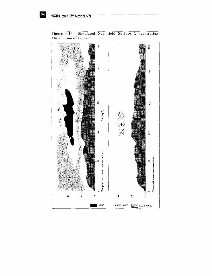
WATER QUALITY MODELING
Figure A.1-4 Simulated Near-field Surface Concentration
Distribution of Copper
E
i -
0 'A-~~A
o o
2 _,0.03 00 0 0.0260.028 0.024-0.0260-03 0.026-0.028 0.024-0.~02

CASE STUDIES OF MODELS APPLIED TO WORLD BANK PROJECTS E
direction for development of a phased approach to wastewater man-agement.
SHANGHAI ENVIRONMENT PROJECT, 1994
The population of the Shanghai municipality in 1991 was about 14million, with some 8 million living in the urban center. Most of thispopulation was served by water drawn from the Huangpu River.The river has played a major part in the development of the city, bothas a route for some 7,000 shipping movements per day between thecoast and the Grand Canal and as a source of water for the many fac-tories which have been built beside the river. The quality of thewater in the river has been degraded by both municipal and indus-trial discharges. The seriousness of the situation was appreciated bythe Shanghai government in the early 1980s; consequently, an intakewas built, upstream of the existing city intakes, at Linjiang, with rawwater fed to the existing treatment works by an enclosed conveyor.However, even this improvement did not allay concern regarding thevariety of industrial discharges upstream of Linjiang and thosewashed upstream to Linjjiang on rising tides. It was thereforedecided to extend the conveyor further upstream. The goal of theproject was to determine where the new intake should be located toprovide a safe drinking water supply.
Summary of the Project
The Shanghai area is very flat, and areas of the municipality arebelow high tide water levels and protected by the Bund; therefore,tidal effects are important. It was decided that a one-dimensionalmodel designed to characterize tidal effects was appropriate toexamine the suitability of a new site at Da Qiao.
The water quality parameters modeled were BOD, ammonia,nitrate-dissolved oxygen, and phenols. Phenols were includedbecause there are high concentrations of phenols in the river andbecause there was an accidental spill of large quantities of phenols in1989.
Rather than simulate a long period of historical records, it wasdecided to select a particular set of hydraulic conditions that wouldrepresent a worst-case scenario, and each model run examined only

U WATER QUALITY MODELING
two tidal cycles. In this way, it was possible to carry out a large num-ber of trial runs in a short period of time.
The natural river flow is largely regulated by controlled dis-charges from Lake Tai. It was therefore possible in principle toreduce the impact of upstream tidal effects by controlling the flow ofthe river at a high level. This approach was tested by using the mode,as were other scenarios, including different sewage and treatmentoptions.
The findings of the modeling process were as follows:
* A paper mill discharging to the river upstream of Da Qiao should beclosed.
* Other discharges upstream of Da Qiao were at acceptable levels.
a Normal discharges from existing factories downstream of Da Qiaowere having a negligible negative effect upon the quality of water at DaQiao.
I Simulation of the phenol spill referred to above revealed that at normalriver flows the impact of the incident would be detected at Da Qiao.
I The effect of increasing the river flow to 300 m3/s would be to eliminatethe risk of a pollution incident in the industrial areas of Minhang andWujing that would adversely affect the water quality.
The findings of the modeling process resulted in the following:
. The paper mill at Zhongjiang was relocated.
a An environmental protection zone was established for the length ofthe river with a width of 10 km. No development in this zone is per-mitted without approval by the Shanghai Environmental PolutionBureau.
* A new intake was constructed at Da Qiao, with a new conveyor of5.4 Mm3/d capacity delivering water to the existing conveyor at Lin-)iang.
* Sewage from the Minhang/Wujing areas was given high priority, andconsideration for its potential adverse effects was given in all worksconstructed under the SSSPII. Thus, failures in treatment or acciden-
CASE STUDIES OF MODELS APPLIED TO WORLD BANK PROJECTS
tal spills in the industrial area will not affect the quality of the Huangpu
River but will be discharged to sea.
Since the operation of the new intake, the quality of drinking
water in Shanghai has noticeably improved, and with the sewerage
works referred to above completed, it has not been necessary to
augment the flows of the Huangpu.
Costs
The options evaluated to solve the drinking water quality problems
were as follows:
* Relocation of the intake Cost - US$253 million
* Advanced wastewater treatment Cost - US$446 million
* Withdrawal of water from the Yangtze Cost - US$1058 million
* Improved local pollution control Cost - US$760 million
The cost of the modeling was about US$200,000; without it, the
cheapest option, relocation of the intake, could not have been select-
ed. This sum represents less than 0.1 percent of the project cost and
less than 0.1 percent of the potential savings.
Conclusions
The highly satisfactory work was largely the result of excellent coop-
eration between the Shanghai government, in particular the staff of
the SEP Project Office, and Mott MacDonald, the international
consultants who were funded by the UK government. Of particular
help were specialists from the He Hai University, who brought
amazingly detailed knowledge of the hydraulics of the myriad water-
ways linking Lake Tai and the Huangpu River.
Lessons to be learned from this most successful case are as follows:
* Define clearly the objectives of the modeling.
* Keep the models as simple as possible.
* Use specialists to make the assumptions and judgments.

g WATER QUALITY MNODELING
MANILA SECOND SEWAGE PROJECT, 1996
To improve the quality of waterways in Metropolitan Manila andManila Bay, the Philippines, and to reduce the health hazards ofexposure to human wastewaters, water supply and sewerage ser-vices needed to be upgraded. Eighty-two percent of the residentialpopulation of Manila use septic tanks for their wastewaters. Theseptage from these tanks will be treated in land-based facilitieswhich are proposed to be constructed during the period 2003-2010.As an interim measure to reduce the human health risks of expo-sure to wastewaters in the metropolitan area, it was proposed thatthe septage be dumped in the open ocean. The locations of theocean dumping, the methods of dumping, and the schedule of thedumpings had to be developed in such a way as to comply with the1972 (with subsequent amendments) "International Convention onMarine Dumping of Wastes and Other Matter" and to minimizethe negative effects of the dumping on the receiving waters. Ini-tially, 1,000 m3 of septage will be dumped in the ocean per day.This volume was expected to increase to 1,500 m3 by year 2001,then decrease as the land-based treatment facilities commenceoperation.
Terms of reference for a water quality modeling study were pre-pared to identify the best locations for the dumping and the methodsof dumping and to examine the potential effects of the ocean dump-ing on coastal areas and recreational beaches. One of the loanrequirements was that environmental impacts be predicted and, ifthese impacts were deemed unacceptable, the project design wouldhave to be changed or other mitigation procedures undertaken toabate the impacts.
Water Quality Modeling Requirements
A hydrodynamic model was required to simulate the three-dimen-sional circulation in Manila Bay caused by surface winds, tides, anddensity gradients for different seasons. The area for the simulationhad to include the proposed dump sites and the shoreline North ofManila Bay (about 90 km north). The hydrodynamic model was tobe used to predict the transport, dispersion, and fate of dissolvedand particulate pollutants from the dump sites for various loadings.
CASE STUDIES OF MODELS APPLIED TO WORLD BANK PROJECTS
Concentrations and zones of settlement were to be predicted andcompared to international environmental quality standards. Cumu-lative effects of dumping at the rates proposed were to be investi-gated. The modeling contract was awarded to the Danish HydraulicInstitute.
Summary of the Project
The model used for this project, MIKE 3 PA, consisted of four ele-ments satisfying the conservation of mass, momentum, salinity, andtemperature and the equation of state relating local density to salin-ity, temperature, and pressure. A brief description of the model ispresented in the Appendix. The hydrodynamic model was a fixedgrid model, and equation solutions were obtained numerically. Themain input data for the model consisted of boundary conditions(two of four boundaries were open, with no data available), topog-raphy, bathymetry, wind climates (shore-based meteorological sta-tions), bottom frictions (no site-specific data were available),loadings, material specifications, dispersion and decay coefficients(no site-specific data were available), velocity depth profiles speci-fications (no site-specific data were available), and simulationperiod. The main two-dimensional model outputs were instanta-neous and averaged circulation vectors, particle concentrations,and erosion/deposition/net sedimentation. Figure 4.15 shows themodel grid and surface circulation vectors. Calibration of themodel parameters used the available water-level data from twosites; meteorology data available from shore weather stations; andCoast Guard data on currents and Manila Bay temperature, salin-ity, and water quality. Because the site-specific data were limited,the model was used to compare scenarios for the same conditions.Figure 4.16 shows these comparisons. Verification of the modelpredictions was not possible because of the lack of site-specificdata: consequently, the quantitative model predictions are not rig-orous.
The model predicted that the depth of solids deposition on theocean floor would be negligible (0.04 mm for the three-year period,for a total of 58,950 tonnes of solids) and therefore would not affectthe fishing grounds. The nutrients provided from the dumpingcould affect the primary productivity in the vicinity of the dump

M WAT~ER QUA~LITY MO~DELING__
Figure 4.15 Simulated Current Velocity Vectors
120 -
80-
AO- jj - -------] 1^l 1 ,- 4-a------
km
site. The 'impact of the dumping will be monitored by measuringturbidity with a Secchi disk. In some instances, bacterial densities atthe recreational beaches and coastal area to the northeast of theocean dumping site were slightly elevated, and a monitoring pro-gram was recommended for those areas. Spills from the bargescould also degrade the bacterial quality in the coastal areas andrecreational beaches. The spill potential was reduced by restrictingbarges to the shilpping lanes and periodic barge inspections.
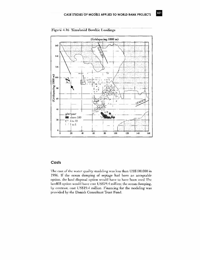
CASE STUDIES OF MODELS APPLIED TO WORLD BANK PROJECTS
Figure A.16 Simulated Benthic Loadings
(Gridspacing 1000 m)
160 _ _ _ \ __
10 -
10 -
80
40 \-_ _X _ _ _ __ _
2--gmly- -- -- -7 --
0 20 40 60 80 100 120 140 160
Costs
The cost of the water quality modeling was less than US$100,000 in1996. If the ocean dumping of septage had been an acceptableoption, the land disposal option would have to have been used Thelandfill option would have cost US$29.4 million; the ocean dumping,by contrast, cost US$19.4 million. Financing for the modeling wasprovided by the Danish Consultant Trust Fund.
WATER QUALITY MODELING
TARIM BASIN II PLANNING PROJECT, 1997, CHINA
The Tarim Basin in northwest China is more than 600,000 square kilo-
meters, with a population of about 6 million. The water resources in
the basin are extensively used for irrigation and consumption A water
resources management study was initiated to investigate methods for
managing the water resources more effectively, in particular to relieve
water shortages that tended to occur during the springtime. In partic-
ular, the following management proposals were to be assessed:
* land reclamation and land improvement, including improvement of irri-
gation system efficiency through land leveling and other measures, and
the introduction of surface drainage for water table control and salt
export;
* improved canal lining, which would result in a reduction in seepage
losses from canals;
* improved on-farm management;
* use of surface reservoirs for resource regulation (although use of thisoption was discouraged); and
* groundwater abstraction, to alleviate water supply shortages during
the spring period and for drainage purposes.
Water Quality Modeling Requirements
Water and salt balance models were required to assess the results of
the various development options. The objectives for the model devel-
opment were as follows;
* to relate the impact of the development options on the surface water
contributions to the Tarim River to the reduction of non-beneficial
losses within the sub-basins and to the salt balance;
* to determine how surface water drainage would affect the salt balance
and how it might reduce non-beneficial losses of salt in the sub-basins;
* to prepare a framework for more detailed modeling of the integrated
surface water and groundwater systems within the sub-basins in the
next phase of the study; and
CASE STUDIES OF MODELS APPLIED TO WORLD BANK PROJECTS
* to make recommendations for future data collection, monitoring, and
river modeling.
Summary of the Project
The models were developed and tested under contract to the Mott
MacDonald consulting firm and specialists from the Xinjiang Agri-
cultural University, Xian University, and Tsinghua University. Fig-
ure 4.17 is a map of the region for which the models were developed;
however, each sub-catchment also had a separate model. The overall
model development components are shown in Figure 4.18. In gen-
eral, the water balance model consisted of river, reservoir, irrigation,
groundwater, and lake modules, with the model formulation in each
module being different. For example, the river module consisted of
inflows, outflows, diversions, exports, gains and losses to groundwa-
ter, evaporation, return flows, and storage changes. The lake module
consisted of inflow from drainage surpluses, inflow from the river
module, evaporation, inflow and outflow to groundwater, change in
lake storage, and other specified outflows. The salt balance model
consisted of reservoir, river, irrigation/groundwater, irrigated and
non-irrigated fields, and lake modules. Like the water balance mod-
els, the salt balance models are formulated differently in each mod-
ule. The models were calibrated "to reach an acceptable agreement
between the observed and simulated water balance components."
Figure 4.19 shows the results of calibration. Once the models were
calibrated, model prediction runs were carried out as follows:
I Sentwitivty analysis. The model parameters were systematically changed
and the effects of these changes on the individual water balance com-
ponents analyzed. Specifically, the sensitivity analysis identified those
water components that were important and established uncertainty
ranges for the controlling parameter to test the impact of a change to
one or several parameters on the water balance.
* Wbat-if/cenarpoa. Model runs are used to obtain a better understanding
of the benefits of certain assumed changes to model parameters on the
water balance. What-if scenarios were used in the runs. For example,
"If I were to increase the depth to the water table, what would be the
effect on capillary losses from the water table and what would be the
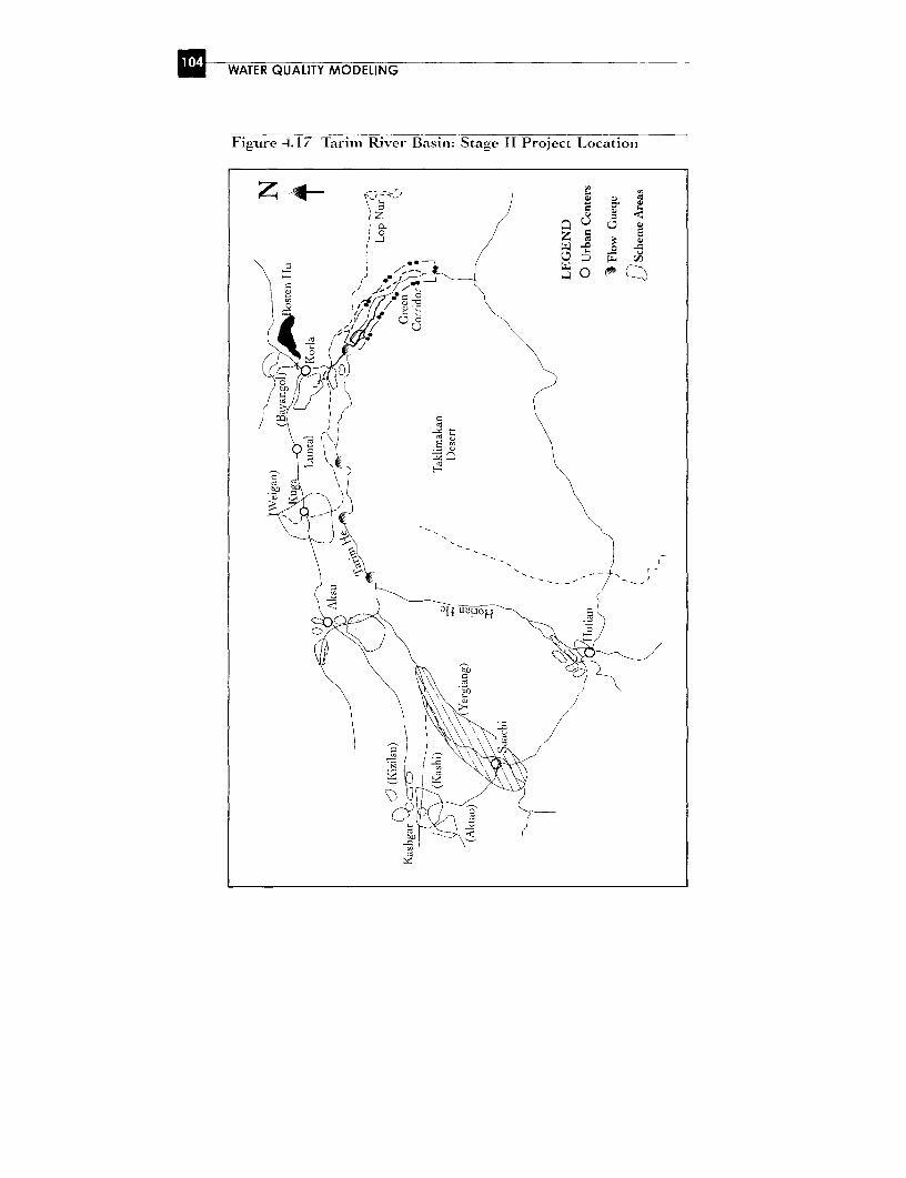
E WATER QUALITY MODELING
Figure -A.17 Tarim River Basin: Stage It Project L,ocation
I LZ 1- - r )c'- IC~~~~~~~~~~~~~~~~~~~~~~~~~~c
0_
CY
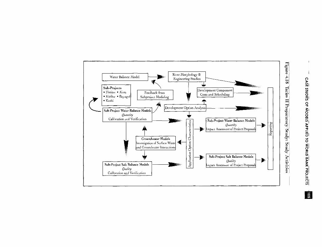
River Morphology & Water Balance Model 1 | .Engineering Studies
Sub-Project s _0* Ilotian * Aksu Feedback from Develop ment Component* Kizilsu * Bayagol SubproectModeling Costs and Scheduling C * Kasha Ch
|Sub-Project Water B alance Models |eelpntOioAayss CalibrationandVerificationDevelopment Option Ana p
Calibration and Verification Sub-Project Water Balance Models DS Oliz 0~~n
Quantity Qunly 5
Groundwater Models uDRi ad Investcgation of Surface Water 0
and Groundwater Interactions O- o; o | Sub-Project Sat Bt e Balance Models C
Sub-Project Salitv Balance lWodels ¢mpact Assesment of Project Proposal, _ -.
Calibrationiand Veri_ .SWaon 0
CA~~~n0
-4
ect Salt Balance Mm
m
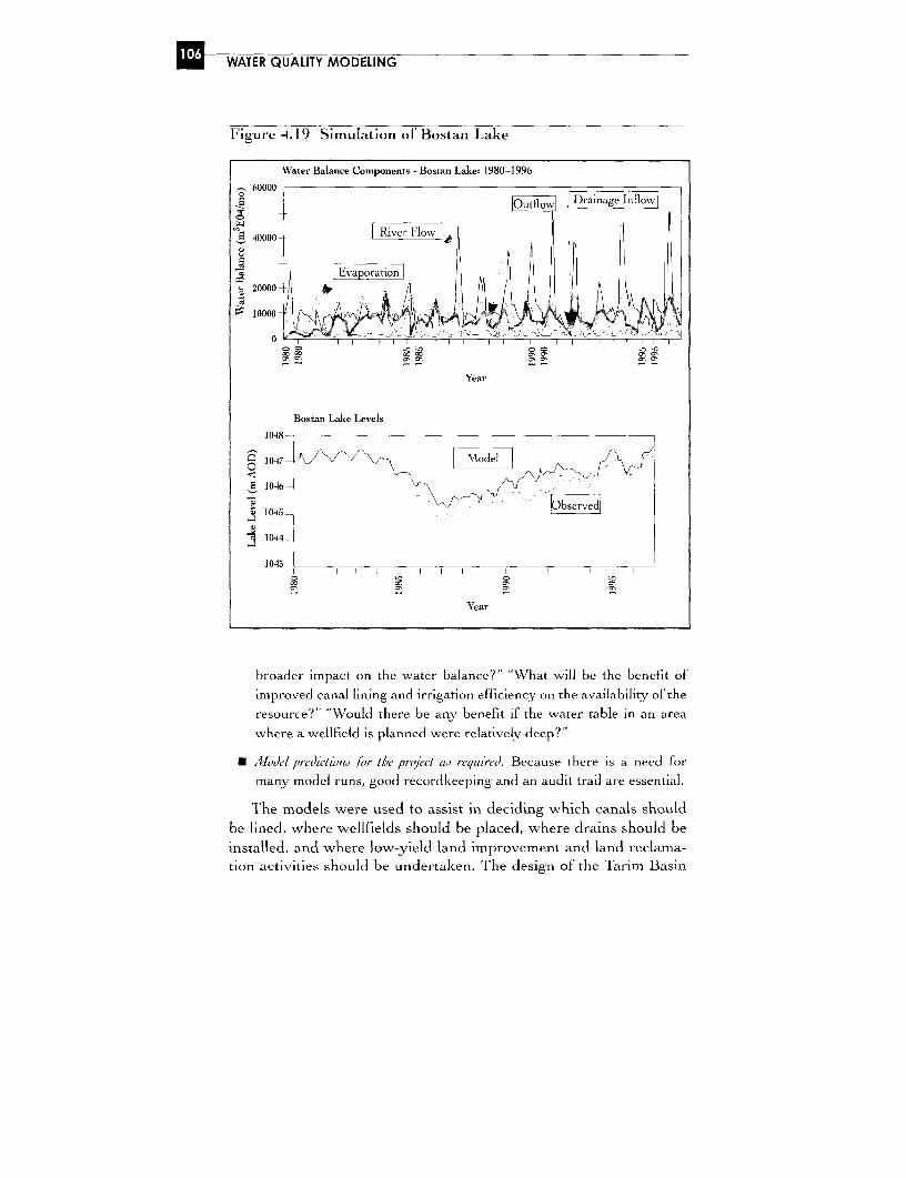
U WATER QUALITY MODELING
Figure -1.19 Simulation of Bostan Lake
Water Balance Components - Bostan Lake: 1980-1996
60000O-tflo | Drainage Inflow
E 40000- River Flov
= 20000 - 1 W K / ;:i - -00io
Year
Bostan Lake Levels
1048-
10417- Model
104
104a_ - bevd
1044_-
1043
Year
broader impact on the wvater balance?!' "What will be the benefit ofirnproved canal li'ning and irrigation ef'ficiency on the availability of theresource?" "Would there be anv benefit if the water table in an areawhere a wellfield is planned w ere relativelv deep?"
* Az1od)el pre-tta7nl fior the prty'ecl a,, req/uired. Because there i's a need formany model runs, good recordkeeping and an audit trail are essential.
The models were used to assist in deciding which canals shouldbe lined, where wellfields should be placed, where drains should be
installed, and where low-yield land improvement and land reclama-tion activities should be under-taken. The design of the Tarim Basin

CASE STUDIES OF MODELS APPLIED TO WORLD BANK PROCTS
II Project (which is presently under implementation) was deter-mined in part on the basis of the model results.
In addition, modeling requirements for the next phase were iden-titied as well as the monitoring and other data collection require-ments to support the prediction models.
Costs
The modeling activities cost approximately US$80,000, which wasfinanced with a Japanese PHRD preparation grant for the TarimBasin II Project.


Appendix
CE-QUAL-W2:A NUMERICAL TWO-DIMENSIONAL LATERALLY
AVERAGED MODEL OF HYDRODYNAMICS ANDWATER QUALITY
Source: Environmental LaboratoryU.S. Army Corps of Engineers3909 Halls Ferry RoadVicksburg, MS 39180-6199Tel: 601-634-3283Program and manual are available on the internet.Contact the above for access information.
Model Hardware Requirements: A recent personal computer with32K RAMVl and 2Meg hard drive with math co-processor with input disk file and line printer or diskfor output.
Professional Expertise Requirements: A university science degreewith experience in hydrodynamic modeling andwater quality modeling.
Receiving Water: Primarily narrow reservoirs.Spatial Characteristics: Two-dimensional laterally averaged.Temporal Characteristics: Dynamic.Water Ouality Parameters Simulated: Dissolved oxygen, biochem-
ical oxygen demand, nutrients, algal bio-mass, tem-perature, indicator bacteria, conservatives andnon-conservatives as well as the interaction of flowand temperature and nutrients and algal productivity.
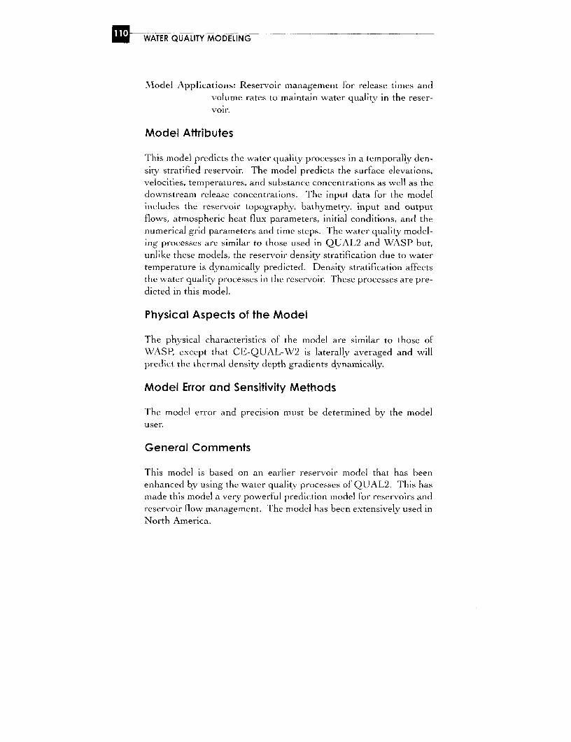
3W _TR QUALITY MODELINNG
Model Applications: Reservoir management for release times andvolume rates to maintain water quality in the reser-voir.
Model Attributes
This model predicts the water quality processes in a temporally den-sity stratified reservoir. The model predicts the surface elevations,velocities, temperatures, and substance concentrations as well as thedownstream release concentrations. The input data for the modelincludes the reservoir topography, bathymetry, input and outputflows, atmospheric heat flux parameters, initial conditions, and thenumerical grid parameters and time steps. The water quality model-ing processes are similar to those used in QUAL2 and WASP but,unlike these models, the reservoir density stratification due to watertemperature is dynamically predicted. Density stratification affectsthe water quality processes in the reservoir. These processes are pre-dicted in this model.
Physical Aspects of the Model
The physical characteristics of the model are similar to those ofWASP, except that CE-OUAL-W2 is laterally averaged and willpredict the thermal density depth gradients dynamically.
Model Error and Sensitivity Methods
The model error and precision must be determined by the modeluser.
General Comments
This model is based on an earlier reservoir model that has beenenhanced by using the water quality processes of QUAL2. This hasmade this model a very powerful prediction model for reservoirs andreservoir flow management. The model has been extensively used inNorth America.

APPENDIX m
CORMIX
Source: U.S. Environmental Protection Agency
Office of Research and DevelopmentEnvironmental Research Laboratory960 College Station RoadAthens, Georgia 30605-2700Send two blank 3.5" HD diskettes. No other costs.Manual available from NTIS.Tel: 703-605-6000, ask for EPA/600/3-90/012, Feb-ruary 1990.
Model Hardware Requirements: Modern PC with mathematics co-processor, input disk file, and line printer or disk foroutput.
Professional Expertise Requirements: A university degree withcourses in hydrodynamics.
Receiving Water: Rivers, lakes, estuaries, and marine coastal areas.Spatial Characteristics: One- or two-dimensional.Temporal Characteristics: Steady state - does not have time as a
variable; however, model can be run repeatedly tosimulate time variability.
WN,ater Quality Parameters Simulated: The initial mixing (mixingzone) of all water quality parameters.
Miodel Applications: All submerged outfalls, either single or multi-ports.
Model Attributes
This model is an expert system that predicts the path and dilutioncharacteristics of a discharged effluent plume for all possible condi-tions. These conditions include positive and negatively buoyantplumes, trapped plumes, bottom-attached plumes, unstable plumes,as well as conventional plumes. Figure CRX I shows the scope of thedifferent conditions that can be simulated in CORMIX. The equa-tions used to predict the plume trajectory path, cross-sectional area,and dilution for each case are presented and discussed in the user'smanual. This model is suitable for all submerged outfalls regardlessof the receiving water. For a particular application, the user suppliesinformation about the discharge and ambient environment. The

X WATER QUALITY MODELING
model returns information detailing the hydrodynamic mechanismscontrolling the flow, dilution, geometric information concerning theshape of the pollutant plume, or flow in the ambient water body, aswell as design recommendations, allowing the user to improve thedilution characteristics of the flow. Figure CRX 2 shows an exam-ple of the model simulation and field observations.
Typical model runs take about five minutes, and a user willrequire two to three days working with the model to understand thevarious functional relationships in the expert system.
Model Error and Sensitivity Methods
There are no discussions of model error and sensitivity methods inthe manuals. The user will have to develop methods for quantifyingthe prediction precision for a particular application. This wouldinclude varying the user input data, either singly or in groups for therange expected in the particular application. Determining the modelprecision could occur as part of the learning process in using themodel.
General Comments
Because the user must provide information on the ambient receivingwater conditions to the model, it is important that site-specific databe available. In particular, the range of values for the input datashould be known. Depth, ambient receiving water currents, andambient depth stratification are the most important input data. Themodel is very useful in the design of multiport diffusers and thedetermination of the best location and depth for the outfall.
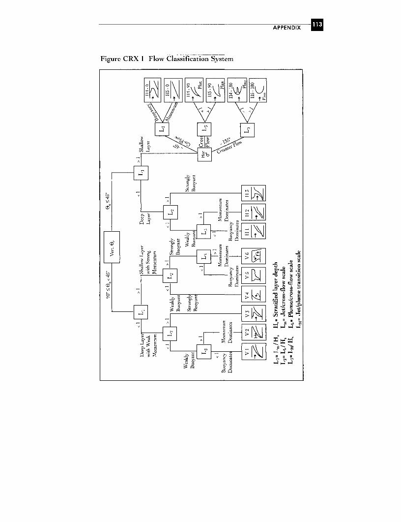
APPENDIX
Figure CRX I Flow Classification System
VI E~~~~~~~~~
CD~~~~~~~~~
X ~~~~~~~~~~ E
so~ ~ ~~ X , 'J 1 '-1
~~~~01~~~~
.4>
.-j r v 3E

WATER QUALITY MODELING
Figur-e CRX 2 Predictions versus Measurements
-o L F,,=20 R=12
40 I L ;
20 :0
-0
O so 100
Distance/D
100 I
D)iluton
10~~~ b,5/ D
4 10 100 200Disa /D
Fan (1967). \iulBoudr*D Dilution D Jet Diameter
* Width bCORMIXI
-CenterlineWVidth 6,3

APPENDIX X
DIVASTBINNIE & PARTNERS
Source: Binnie & PartnersGrosvenor House69 London RoadRedhill, SurreyUnited KingdomTel: 44-1737-774155Fax: 44-1737-772769Details on the model are available at the addressabove.
Model Hardware Requirements: Unknown because it is a propri-etary model, but a recent personal computer with32K RAM and 2Meg hard drive with math co-processor would be appropriate.
Professional Expertise Requirements: User should have a sciencedegree and be knowledgeable in modeling tech-niques and have an appreciation of modeling physi-cal processes.
Spatial Characteristics: Two dimensions.Temporal Characteristics: Dynamic.Water Quality Parameters Simulated: DIVAST (Depth Integrated
Velocity And Solute Transport) -Soluble sub-stances, including indicator bacteria.
Model Applications: Wide rivers, lakes, estuaries, and coastalregions.
Model Attributes
This model consists of the dynamic partial differential hydrodynamicequations in two dimensions, continuity equation, and the mass bal-ance equation. These equations are coupled and solved numericallyon a horizontal grid with variable cell sizes using an alternatingdirection implicit scheme (Figure 4.6). The outputs from the modelinclude water surface elevation, current speed, and direction andconcentration. The hydrodynamic model will accept continuouslyrecorded wind, water depth, and current data. The model gridrequires the topography and bathymetry. The continuously
X WATER QULAITWYMODELING
recorded wind, water depth, and current data near the model bound-aries were used as input boundary conditions for the model calibra-tion. In the calibration process, the bottom roughness coefficients,surface wind drag coefficients, eddy coefficients, and model timesteps are adjusted so that predicted water depths and currents matchcontinuously recorded depths and currents at interior locations onthe grid (Figure 4.7). The solute calibration consisted of adjustingthe dispersion coefficients to match measured bacterial densities.Site-specific data from tracer studies on the rising and falling tidesand laboratory measurements of the bacterial mortality rates werealso used in the model calibration (Figure 4.8).
Model Error and Sensitivity
Numerical dispersion can be computed from the grid size, velocity,and time steps used. The model predictions of depth, currents, andbacterial densities at various locations on the prediction grid arecompared to continuously recorded data in the calibration process;consequently, the precision of the model predictions should be rea-sonable. The sensitivity of the model can be determined usinganother data set for verification. If continuously recorded data arenot available, a sensitivity analysis can be carried out on the requireddata input parameters.
General Comments
The model was used to assess different locations and levels of treat-ment for two large outfalls for Bombav. The modeled area had theshore as one boundary, and the other three boundaries were opencoastal waters. Numerical prediction models for a coastal area withthree open boundaries are very difficult; therefore, Binnie & Part-ners used extensive site-specific continuously recorded data for themodel development.

APPENDIX X
HYDROLOGICAL SIMULATION PROGRAM-FORTRAN (HSPF)
User's Manual for Release 8.0
Source: U.S. Department of CommerceNational technical Information Service5285 Port Royal RoadSpringField, VA 221161Tel: 703-605-6050Reference: EPA/600/3-84-066, June 1984
orEnvironmental Research LaboratoryU.S. Environmental Protection Agency960 College St. RoadAthens, Georgia 30605.(706) 355-8000Paper copy of the user manual is available fromeither address above. The program is free of chargefrom the Athens address above, but the request mustbe accompanied by six HD 3.5" disks.
Model Hardware Requirements: RAM 512 Kbytes, diskette, harddrive with more than 3Meg, numeric co-processor,DOS, and ANSI FORTRAN.
Professional Expertise Requirements: User should have a sciencedegree, be knowledgeable in modeling techniques,and have an appreciation of the modeling physicalprocesses. HSPF is a large, relatively sophisticatedhydrologic hydraulic and water quality simulationprogram that does not include a sewer network.
Spatial Characteristics: Two dimensions.Temporal Characteristics: Dynamic.Water Ouality Parameters Simulated: Dissolved substances, sus-
pended solids, dissolved oxygen, nutrients, and indi-cator bacteria. The water quality parameters arelinked to the runoffs generated in the hydrologicalmodules.
Model Applications: Predicts runoff from rainfall and topographi-cal information for the catchment.

E WATER QUALITY MODELING
Model Attributes
This is a complex model that predicts runoff in real time from rain-fall data. The SWMMI\I extended HSPF's capabilities to urban areas.SWMM is similar to HSPF in structure. HSPF has many modulesthat the model user can select for a particular application. The modelhas been extensively used to predict runoff and runoff quality. Themanual contains extensive information on the receiving water qual-ity processes; however, these processes are common to most models.Like the SWiMJM model, HSPF can be used as a black box runoffprediction model with an abbreviated input data set if calibrationand verification data are available.
Model Error and Sensitivity
The accuracy of the runoff prediction from HSPF should be similarto SWMM's. The error can be determined by using verification dataand/or using sensitivity analysis for the user provided coefficientsand rate constants.
General Comments
HSPF is one of the early runoff prediction models developed. Thequality components of the model are all linked to the washoff orrunoff components of the model. The model has a good suspendedsediment kinetics module (Figure HSP 1 from the user's manual).The nitrogen and phosphorus processes considered in the model areshown in Figures HSP 2 and HSP 3, respectively. There is also areservoir quality module (Figure HSP 4). While it is possible toselect the appropriate model module, the hydrological module out-puts must be available. This model is useful for river basins, whichare largely rural.
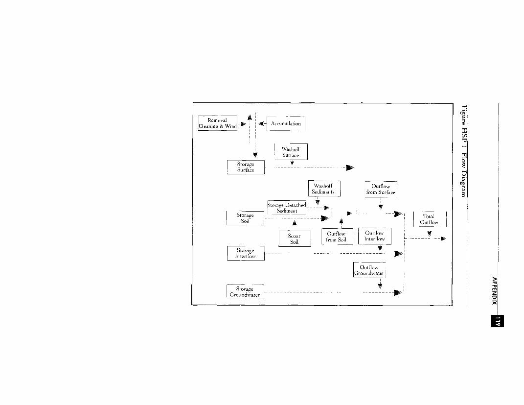
Removal .
Cleaning & Wind b j - Accumulation
WashoffW Surface |T
St-orage l--- | Sutorage _- --- _-- _--- __- __- _.--
| Surface |>t
|Washoff | |Outflow |4
Storage Detached__ - - -
F Storage I Sediment I-- ----- Tta
Soil 48 Outflow
Storage-- -_---
Interfiow_-- ---------
OutflowGroundwater
V~~~~~~~ X
Grounci~~~~$ater - ------------
F - -s -t ,.g e - - - - - - -- - - - - - - - - - - - - - - - - - - -
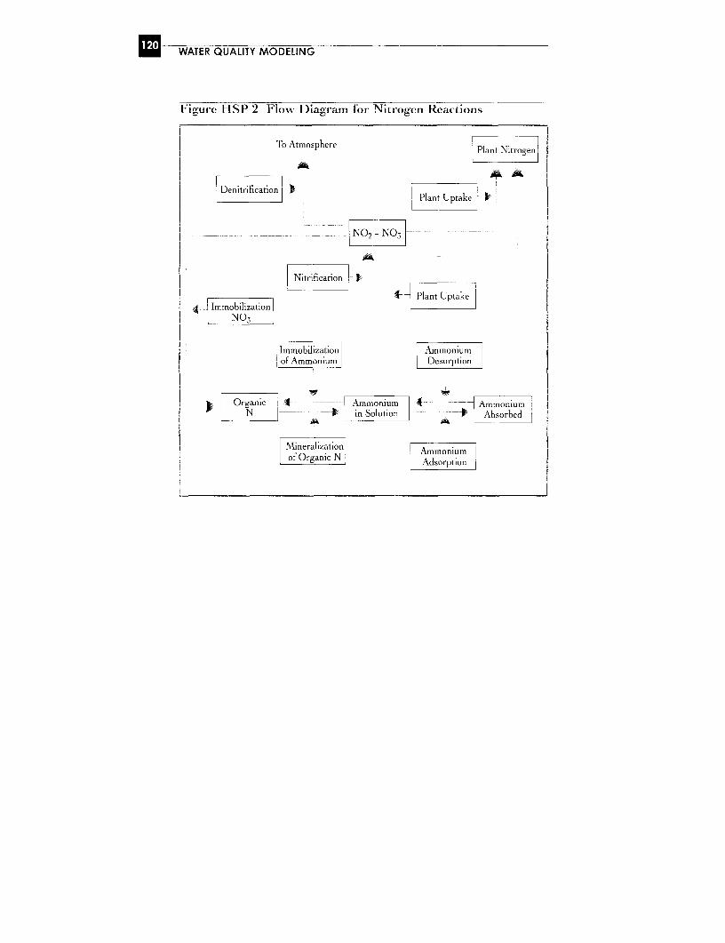
E3 WAT7ERQUALITY MOD ELING
Figure HSP 2 Flow Diagram for Nitrogen Reactions
To Atmosphere EPlnt Nitrogen
Denitrification i f Plant Uptake |1
e|trfico Nitrification
i ;~~~~~~~~tX Plant l,ptake4 Immobilization
NO5
Immobilization Ammoniumof Ammonium Desorption
Organic I monu AmmoiumN i u Absorbed
Mineralization Ammoniumof Organic N Adsorption

PlantPhosphorus (P)
PlantUptake
Phosphate | Desorption
Im onobilization
Organic Phosphate Phosphate Pp~~~~ in Solution 4Absorbed
A~~~~~~~~~~~~~~~~~~~
3.
Organic P Adsorption
Mineralization Phos,phate>T-uzX
E

E WATER QUALITY MODELING
Figure HSP -4 Flow Diagram for Solids
Clay Inflow
- - Absorption =Suspended -u
Desorption Clay
A
___ O~~~n- - Suspended --
Silt
OnSuspended c
4--------a Sand
C1 / /X // BEDw
f-a On Bed Sand |
t }iOOn Bed Silt
~~t-~- ~ ~~- ~ > On Bed Clay

APPENDIX
MIKE SYSTEM
Source: Danish Hydraulic InstituteAgern Alle 5DK - 2970, HorsholmDenmarkProprietary model. Technical Reference Manualsare available.
Model Hardware Requirements: The minimum hardware require-ments are a 586 computer with mathematical proces-sor, 32k RAM, 5 Gbyte hard disk, and printer andplotter.
Professional Expertise Requirements: Professional with experi-ence in numerical modeling, hydrodynamics, andwater quality.
Receiving Water: MIKE SYSTEM consists of different models(MIKE I l, MIKE 21, MIKE 3, MIKE SHE,MOUSE and MIKE BASIN); consequently, themodels can be used for rivers, lakes, estuaries, andcoastal regions.
Spatial Characteristics: One, two, or three dimensions. MIKE 11is a one-dimensional modeling system, MIKE 21 atwo-dimensional modeling system, MIKE 3 a three-dimensional modeling system, MIKE SHE an inte-grated hydrological modeling system, MOUSE anintegrated modeling package for urban drainage andsewer system, and MIKE BASIN an integratedwater resources management and planning system.
Temporal Characteristics: Dynamic and time-variable.Water Quality Parameters Simulated: Water level, velocity, tem-
perature, dissolved oxygen, biochemical oxygendemand, nitrate, ammonia, dissolved conservativesubstances (e.g., salinity), and dissolved substanceswith a decay term (e.g., indicator bacteria).
Model Applications
MIKE 11 NAM ( the hydrological module of MIKE 11 system):Data inputs required are catchment topography, precipitation,
E WATER QUALITY MODELING
potential evapo-transpiration, and temperature. Model input param-
eters required are overland flow coefficient, interflow time constant,
threshold value overland flow, threshold value interflow, time con-
stants, specific yield of groundwater reservoir, time constant base-
flow, storage including snow, surface, lower zone, and groundwater.
Model outputs include daily runoff, variation of soil moisture con-
tent, and ground water recharge.
MIKE 11 HD (the hydrodynamic module of MIKE 11 system):
The hydrodynanic model is for rivers based on the numerical solu-
tion of the coupled partial differential equations for continuity,
momentum, and dissolved substance dispersion and transport.
Data inputs required are river divided into reached, river cross-sec-
tional data, upstream boundary conditions, and tributary and other
discharges and withdrawals. Model input parameters required are
time step and duration of simulation, bottom roughness coefficients
for channel and flood plains, initial conditions, dispersion coeffi-
cdents, and first-order decay rate. Model outputs include river
water level, river flow, and accumulated flow and concentrations of
dissolved substances, either conservative or affected by first-order
decay only.
MIKE 11 WO (the water quality module of MIKE 11 system):
Data input required are river flow and water level from the hydro-
dynamic model, loadings from upstream boundary, tributaries and
discharges, and initial conditions in the river. Model input parame-
ters required are degradation constants, sedimentation and resus-
pension rates, photosynthesis and respiration rates, critical velocities
for sedimentation, sediment oxygen demand, re-aeration rates, oxy-
gen yield and uptake rates for ammonia and phosphorus, reaction
rates for nitrification and denitrification, and adsorption/desorption
of phosphorus on suspended solids. Model outputs include dis-
solved oxygen, biochemical oxygen demand, ammonia, nitrate, phos-
phorus, and temperature at river cross-sections.
MIKE 21 HD (the dynamic two-dimensional hydrodynamic module
of MIKE 21 system): The model can be used for rivers, lakes, estu-
aries, and coastal regions based on the numerical solution of the cou-pled partial differential equations for continuity, momentum, and

APPENDIX
dispersion and transport of dissolved substance. Data inputsrequired are similar to MIKE 11 above but in two dimensions plussome other inputs like the velocity (flux) distribution and bathyme-try. Model input parameters required are similar to MIKE 11.Model outputs include water levels, depth-averaged velocity vectors,flow, and accumulated flow.
MIKE 21 WQ (the dynamic water quality module of MIKE 21 sys-tem): Data inputs required include the output from the hydrody-namic model. MIKE 21 WO Model inputs parameters required aresimilar to MIKE 11 but in two dimensions. Miodel outputs are simi-lar to MIKE 11 but in two dimensions.
MIKE 3 PA (one of the sediment/particle transport module ofMIKE 3 system): The model can simulate the transport and fate ofdissolved and suspended substances discharged or accidentallyspilled into rivers, lakes, estuaries, coastal areas, or open seas. Thetransport can be in two or three dimensions. This is a Lagrangianmodel for the advection and dispersion resulting from randomprocesses of released uniformly distributed particles. It requires cur-rent velocities and water levels in time and space for the computa-tional grid. The model can predict any conservative and decayingsubstances. Model inputs include bathymetry, bed friction coeffi-cients, source data, wind data, dispersion coefficients, velocity depthprofiles, and decay coefficients. The following discussions do notrelate to a Lagrangrian model.
Note: the following three models are not DHI MIKE systemfamily.
TIDEFLOW-3D: Dynamically simulates currents, dissolved solids,and temperature.
XXFLOW-3D: Simulates advection and transport of mud and sin-gle pollutants and interacting water quality parameters using theoutput of TIDEFLOW-3D.
XXPLUM-3D: Random walk models for sediment and dissolvedsubstance plumes.

X WATER QUALITY MODELING
Model Attributes
The area must be divided into catchment areas. Topographical mapsand other information related to runoff must be obtained for thecatchment areas. The rivers are divided into branches of similar
hydraulic characteristics (alignment, river cross-sections, slope, and
river bottoms). In the case of the two-dimensional model, the area is
divided into grids. Model predictions are for the branch boundaries
or grid intersections. The partial differential equations are solved
numerically using an implicit finite difference scheme on the compu-
tational grid. The point and non-point discharges must be quantified
and properly located in the river reach or grid. Similarly, upstream
boundary and initial conditions must be defined as well as the initial
water quality concentrations.
Physical Aspects of the Model
All predicted parameters are dynamic or time-varying. The user can
select among six levels of water quality descriptions, from the simple
dissolved oxygen and biochemical oxygen demand to a model that
includes the most important dissolved oxygen processes. An exampleof the model setup is shown in Figure 4.13.
Dissolved Oxygen
The various dissolved oxygen processes included in the two-dimen-
sional model are shown in Figure MVIK 1. The processes shown in
Figure MIK I are superimposed on the simulations from the hydro-
dynamical model.
Nutrients - Nitrogen and Phosphorus
The nitrogen processes in the model are shown in Figure MIK 2.
The phosphorus processes in the model consist mainly of phospho-
rus adsorption and desorption from suspended sediments. These
processes are superimposed on the simulations from the hydrody-
namical model.
Two-Dimensional Model
The velocity vectors are simulated in two dimensions. Figure 4.15 is an
example of the simulation of the maximum ammonia concentration.
APPENDIX E
Error and Sensitivity Analysis
There are no recommendations or discussion for determining theerrors and sensitivity of the model input parameters. The sensitivityof the model simulations to various input parameters is useful to themodel user for the model calibration process. The model user can userecognized statistical methods to conduct a tailored sensitivity analy-sis and determine the sensitivities.
Calibration
Model calibration is discussed in the Chongqing report. A calibra-tion data set is selected and the model parameters adjusted to obtaina match between measured and simulated values. This process is car-ried out for water levels, flows, accumulated flows, temperature, andthe other simulated water quality parameters. The parameters thatcan be adjusted in the calibration process are identified in the modeldocumentation.
Verification
Model verification is discussed in the Chongqing report. In thisprocess, the calibrated model simulated values are compared withanother data set. Any significant differences are investigated. If thedeviations are unacceptable large, it may be necessary to recalibratethe models.
General Comments
The model in its two-dimensional form is very complex, requiringmany different data inputs. The complexity of the model was appro-priate for the Chongqing project, where the receiving water consistsof two major rivers with two tributaries upstream of the ThreeGorges Dam. These rivers have 50 major domestic wastewater out-falls, 12 major industrial outfalls, and 15 non-point source loadingsin the Chongqing region. There are also large loadings to theYangtze River upstream of the Chongqing area. However, complexmodels are more difficult to calibrate and verify because of the num-ber of input parameters and data that must be provided to the model.In the case of Chongqing, many of the simulated values were within5 percent, and some differed by 200 to 300 percent. It is important

E 3WATE ~RQU ATMODELING _-
that the model user know in what instances the simulated and meas-ured values have significant differences and interpret the simulationsin an appropriate manner. If the model is correctly formulated, it canbe argued that it must be possible to calibrate the model properly ifthe accurate calibration data are available. Usually there are insuffi-cient data for the calibration process and, even if these data are avail-able, the calibration process may still not be perfect because of thenumber of different combinations of input parameters that must beassessed and analyzed. Time and cost usually limit the calibrationprocess.

SourcesBOD 5 -Susp., BOD 5-Diss., NHs
Reaeration _
Dissolved / ~BOD5 DisscDissolved _ Degradation 0Org. _MatterRespiration
Suspended B tg 'BODs susp.O
( DegradationSedimented \Adsorption J .Resuspension Photosynthesis
-L- * __PlantsSedimentedOrg. Matter
BOD5 sed. Respiration >Degradation ( _ Nitrification
z
_ . ~~~~~~~~~~~~~~~~~~X
0

rn-Pollution Sources Rainfall.(BOD, Nitrogen)
Organic Matter Ammonification NHo/NH Nitrification 01~~~~
------ Uptake in
A Algae & Plants
Sedimentation I
t Resuspension Algae Plants
APPENDIX
QUAL2E & QUAL2E-UNCAS(6 APRIL 1999)
Source: U.S. Environmental Protection AgencyOffice of Research and DevelopmentEnvironmental Research Laboratory960 College Station RoadAthens, Georgia 30605-2700Send two blank 3.5" HD diskettes. No other costs.Manual available from NTIS.Tel: 703-605-6000; ask for EPA/600/3-87/007, May1987.
Model Hardware Requirements: PC with at least 256K memorywith input disk file and line printer or disk for out-put.
Professional Expertise Requirements: A university degree withcourses in hydrodynamics and environmental engi-neering.
Receiving Water: Primarily narrow rivers with tributaries.Spatial Characteristics: One-dimensional - downstream direction.Temporal Characteristics: Steady state for one solution - does not
have time as a variable; however, model can be runrepeatedly to simulate time variability.
Water Ouality Parameters Simulated: Dissolved oxygen, bio-chemical oxygen demand, nutrients, indicator bacte-ria, conservatives, and non-conservatives.Uncertainty analysis is available for model parame-ters in the form of sensitivity analysis, error analysis,or Monte Carlo simulation.
Model Applications: To determine the impact of waste loadingsfrom both point and non-point sources on the receiv-ing water quality.
Model Attributes
The river is divided into reaches that have similar hydrauliccharacteristics (maximum 25 reaches). Each reach is dividedinto computational elements of equal length. Elements at theheadwaters, at junctions, at inputs or withdrawals, and the last
E WATER QUALITY MODELING
element are identified in the model (Figures QUAI and OUA 2).
The one-dimensional advection-dispersion mass transport equa-
tion is numerically integrated over space and time for each water
quality constituent. Equations are solved by finite difference
methods.
Physical Aspects of the Model
The river flow is assumed constant at the headwater element. The
mass transport equation requires that stream cross-sectional area,
mean stream velocity, downstream dispersion coefficient, and the
volume of water in the element be known. The mean velocity, cross-
sectional area, and depth in the reach are determined using the
power functions of the flow or particular cross-sectional data (e.g.,
trapezoidal, rectangular, etc.). Three different options can be
selected for determining the downstream dispersion, and some of
these are dependent on the channel roughness. A table of channel
roughness is provided in the manual, and some typical dispersion
coefficients in rivers are provided in a table. The rivers are U.S.
rivers, but details on the river depth, width, and mean velocity are
provided in the table so that these data can be considered universal.
Primary productivity
Algal bio-mass is determined as a function of the chlorophyll a meas-
urement. Productivity is determined from light functions (three
options) or light averaging functions (four options) and algal self-
shading.
Algal-limiting nutrient relationships are developed using
Michaelis-Menten ratios.
Nitrogen cycle
The equations for organic nitrogen, ammonia nitrogen, nitrite nitro-
gen, and nitrate nitrogen are developed and solved. These relation-
ships require algal bio-mass.
Phosphorus cycle
The equations for organic phosphorus and dissolved phosphorus are
developed and solved. Algal bio-mass is an important component of
the equation.
APPENDIX
Carbonaceous BOD
The equations for BOD assume a first-order reaction to describe thede-oxygenation of BOD. This consists of a rate reduction, which istemperature-dependent, and settling of the BOD particles.
Dissolved oxygen
The rate of change of dissolved oxygen depends on re-aeration, pho-tosynthesis, oxygen of the incoming flow, oxidation of carboneousand nitrogenous organic matter, and benthic oxygen demand andrespiration.
Eight different methods exist for determining re-aeration as wellas a special re-aeration method for dams. Default values for all of thecoefficients are presented in a table in the manual. Figure 2.1 showsthe dissolved oxygen processes included in the model.
Indicator bacteria
Bacterial densities are simply determined using a first-order decaysuperimposed on the advection and dispersion predictions.
Temperature
Temperature is determined by a heat budget which considers solarradiation (short- and long-wave and reflection), convective heat,evaporation losses, and heat flux. This component of the model hasbeen found to be very effective.
Tabular values of the default options for all the coefficients in themodel are provided, as well as a range of measured values.
The manual contains good schematics that are helpful for visualizinghow the model functions. Details on the finite difference methodused to solve the equations are well presented in the manual.
Model Error and Sensitivity Methods
The model error and sensitivity methods are presented as an optionin the model application. The three types of error analysis are as fol-lows:

Xl WATER QUALITY MODELING
Sensitivity analysis: In the model, the sensitivity of the model predic-tions can be assessed single inputs or groups of inputs or factorial design.
First-order error analysis: It is possible to obtain a table of sensi-tivity coefficients (normally distributed) as a percentage of change inthe output variance. It is also possible to obtain the components ofvariance of each output variance as the percentage of the outputattributed to each input variable.
Mvlonte Carlo simulation: It is possible to run the model in a MonteCarlo simulation mode.
An excellent table is provided on the model uncertainty associatedwith the variance of the input variables. As a typical percentage,these can be summarized as follows:
Temperature 2-3%BOD 0-20%Dissolved oxygen 5- 10%Nitrogen 15-30%Phosphorus 15-40%Algae 10-25%Bacteria 0.2-0.35 logConservative 5-10%C-ohesive sediments and flocs 50-100%
The user manual is easy to use and is presented in a step-by-stepmanner.
General Comments
OUAL2 is one of the most extensive water quality prediction mod-els used. The configuration of the model is flexible, so that the usercan change it for special applications. This model is so popular thatit has been incorporated in many other models in one form oranother. The model can be used with very little site-specific data,which is its advantage and disadvantage, because the model can beused by personnel with no expertise in receiving water quality,hydraulics, or modeling/prediction.
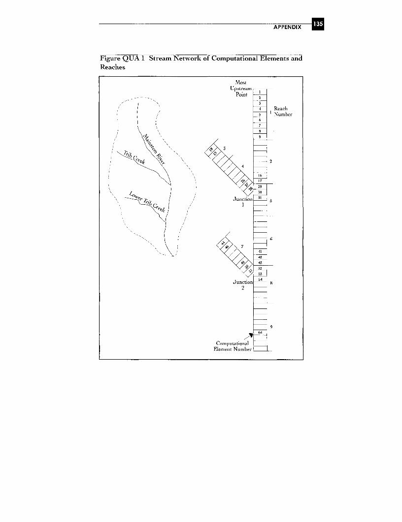
APPENDIX U
Figure QUA 1 Stream Network of Computational Elements andReaclhes
MostUpstream
Point 12
4 Reach5 Number6
78
9
3~~~~~~~
c~~~~~~~~~~~~~~~~~
16
' 729
Junction 20
6
~s 7412
4 .2
N52
53
Junction 548
2
9
CoDmputationaElement Nume

- I
zX
11 -
/ I~~~~~~~
t '° lo \9zn f\ : :~~~~~~~~~~~~~~~~
8 F ' | 0 5 < \ eN w
" 4 > !X: ; i' ni~~~~~~~~~7
X,,,, v 1,
APPENDIX
STORM WATER MANAGEMENT MODEL (SWMM)VERSION 4 PART A: USER'S MANUAL
Source: U.S. Department of CommerceNational Technical Information Service5285 Port Royal RoadSpringfield, VA 221161Tel: 703-605-6050Reference: EPA/600/3-88/001a, June 1988
orEnvironmental Research LaboratoryU.S. Environmental Protection Agency960 College St. RoadAthens, Georgia 30605.Paper copy of the user manual is available from theaddresses above. The program is free of charge fromthe Athens address above, but the request must beaccompanied by two HD 3.5" disks.
Model Hardware Requirements: RAM 512 Kbytes, diskette, harddrive of 3Meg or more, numeric co-processor, DOS,and FORTRAN 77.
Professional Expertise Requirements: User should have a sciencedegree, be knowledgeable in modeling techniques,and have an appreciation of modeling physicalprocesses. SWMM is a large, relatively sophisticatedhydrologic, hydraulic, and water quality simulationprogram.
Spatial Characteristics: One dimension.Temporal Characteristics: Dynamic - time is a variable.WVater Ouality Parameters Simulated: None. SWMM is set up to
link with WASP4 and DYNHYD.Model Applications: Predicts runoff for complicated urban areas
with sewer systems from rainfall and topographicalinformation in the catchment.
Model Attributes
This is a very complex model that predicts runoff in real time fromrainfall data for an urban area. The model has been extensively used

E WATER QUALITY MODELING
for urban areas and is one of the best models for predicting runofffrom urban areas with a well-developed sewer system. The modelcan be used as a black box runoff prediction model with minimalinput data if calibration and verification data are available. FigureSWM 1 shows the components of the model; Figure SWM 2 showsa typical setup for a model input.
Model Error and Sensitivity
The quantity prediction from SWMM may be very accurate, withlittle calibration because of the model structure. The error can bedetermined by using verification data.
General Comments
The model is very useful for generating flows in pipe networks inurban areas. The model can handle any hydraulic cross-section aswell as different flow regimes (Figure SWM 3). The model has goodhydraulic and sediment dynamics sub-routines for open channelflow and good backwater computations in the EXTRAN Addendum(EPA/600/3-88/OOlb). The model has a dry weather flow module,which is very useful for water quality management because it is thedry weather flow periods that frequently stress the receiving waterquality. The manual is easy to use, and the model processes aredescribed well.
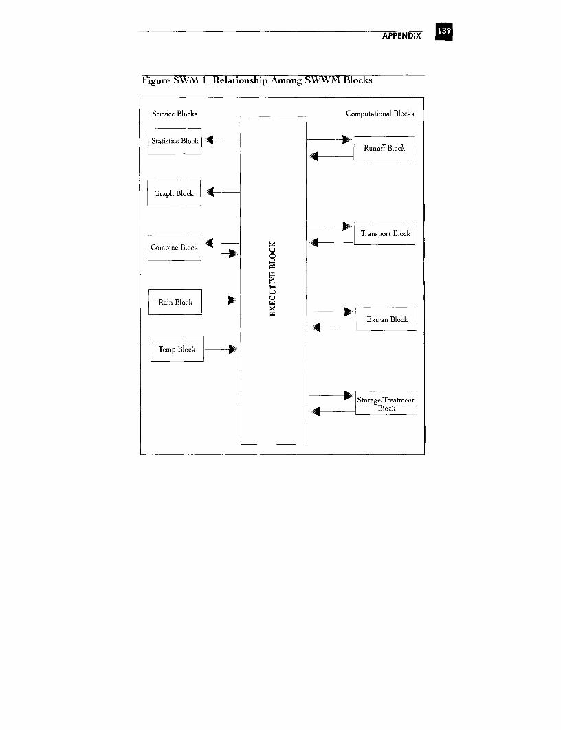
APPENDIX
Figure SWM 1 Relationship Among SWVWM Blocks
Service Blocks Computational Blocks
Statistics Block |4- ----
Combine Block ~ ~ ~ ~ ~ ~ ~ ~ unffBlcGraph Block|
|Transport Block
Combine Block U O
Rain Block
Extran Block
Temp Block
Storage/TreatmentBlock
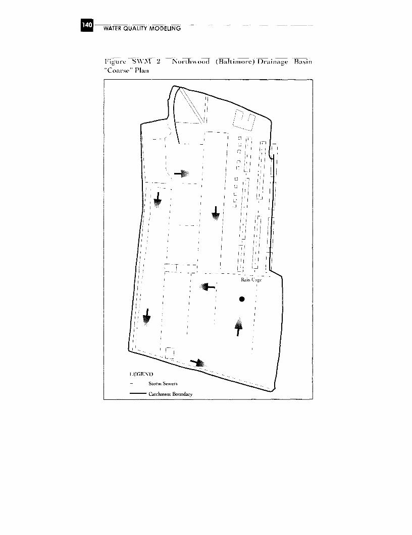
WATER QUALITY MODELING
Figure SN'.\l 2 Northw-ood (Baltimore) [Drainage Basin
"Coarse" Plan
._-
Rain Gagc
I /~~~~~~~~~~~~~
LEGEND e B
-- - Storm Sewers
Catchment Boundary
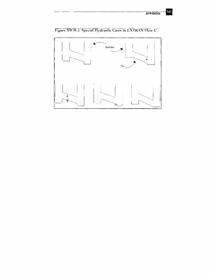
APP EN DIX A3
Figure SWMNI 3 Special Hydraulic Cases in EXTRAN Flow C
I.Wanholes
Pipe
X 2 - L<>--X\C~~~--
WATER QUALITY MODELING
TRISULA - DELWAQDELFT HYDRAULICS
Source: Delft HydraulicsRotterdamseweg 185P.O. box 1772600 MH DelftThe NetherlandsTel: 31 15 2858585Email: [email protected] on the models are available at the addressabove.
Model Hardware Requirements: Unknown because it is a propri-etary model. Presumably, a recent personal com-puter with 32K RAM and 2Meg hard drive withmath co-processor would be appropriate.
Professional Expertise Requirements: User should have a sciencedegree, be knowledgeable in modeling techniques,and have an appreciation of modeling physicalprocesses.
Spatial Characteristics: Two and three dimensions.Temporal Characteristics: Dynamic.Water Quality Parameters Simulated: Inorganic and organic sedi-
ment kinetics, nutrient kinetics, phytoplankton,nitrification and denitrification, mineralization, oxy-gen and biochemical oxygen demand, heavy metals,indicator bacteria, and oils.
Model Applications: Lakes, estuaries, and coastal regions.
Model Attributes
This model consists of equations that are solved numerically usingfinite element techniques. Figure TRI 1 shows the model modulesand the input and output data. TRISULA is the hydrodynamicmodel and DELWAO the water quality model. Figure TRI 2 showsthe water quality substances and processes included in DELWAQ.Figure TRI 2 clearly shows that the processes simulated are com-prehensive and include surface processes like re-aeration, denitrifi-
APPENDIX A
cation, and volatilization as well as the bottom sediment processeslike sedimentation, mineralization, resuspension, and burial. Thewater processes include all the major components of the primaryproductivity system as well as dissolved and detritus of the nutrients,spill, and first-order decay processes. Details on the operation andapplication of the models are available from the owners.
Model Error and Sensitivity
The total concentration levels are calibrated as well as the waterquality and ecological processes. The various model coefficients andrate constants are systematically adjusted in the calibration process.Details on the calibration process are discussed in the project reportfor Hangzhou Bay. Figure 4.12 shows an example of the calibrationprocess. In the figure, the differences between the simulated andmeasured salinities in the bay are presented. The calibration process,coupled with some sensitivity analysis for the user-provided coeffi-cients and rate constants, should quantify the precision of the modelsimulation for any application.
General Comments
The models have been extensively used on large water resource proj-ects throughout the world. Further details on the models can beobtained from Delft Hydraulics.
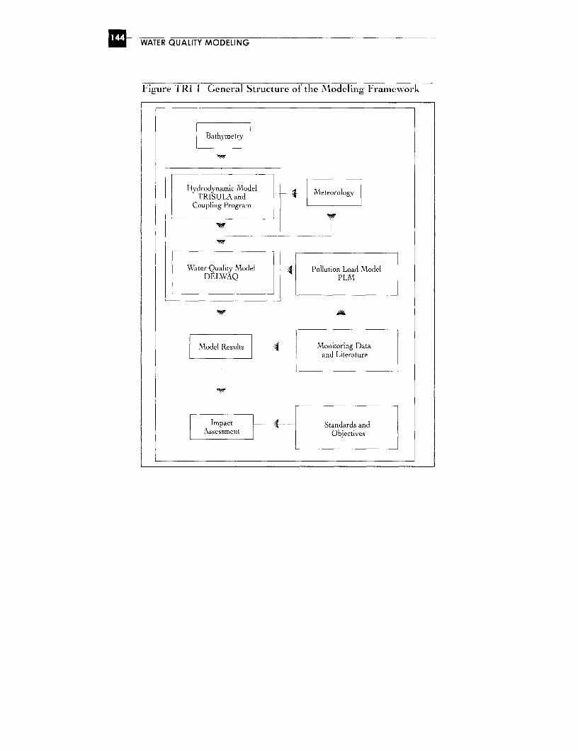
C WAT~ER QUALITY MO~DELIN~G
Figure TRI I General Structure of the Modeling Framework
Bathymetry
Hlydrodynamic Model Meero'TRISULA and ,
Coupling Program
w~~~
Water Quality Model 4 Pollution Load ModelDELWAQ PLM
{ Model Results 4- M^onitoring Dataand Literature
| Impact 4 Standards andAssessment Objectives
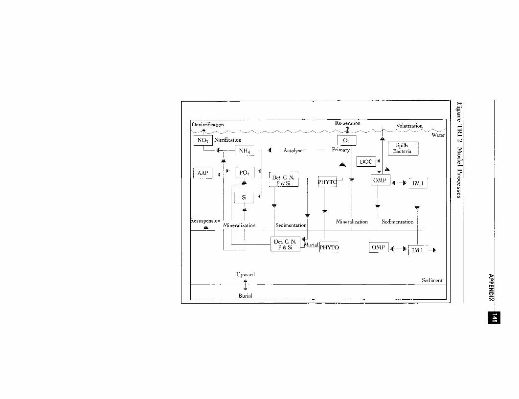
Denitrification Re-aeration Volatization
t-< -'\-~ --- ~ - -- '--'<--~~ ' -- '--4 -- -1 ~-~<~^~-^Wa-ter 5.
NO3 Nitrification 02spills
L~ zxx NH4:3 -- 1 Autolyse - Primary Bacteria
AAP X> P0 4 3 <i3HC + J~Dt.C,
r Si HY IM
Resuspension Mineralization Sedimentation Mineralization Sedimentation
| Det. C, N, | M I |P & Si _ HYT 3OMP - M -
UpwardSediment
mBurilz
_ ~~~~Burial C)X
WATER QUALITY MODELING
WQRRSWATER QUALITY FOR RIVER-RESERVOIR SYSTEMS
Source: Hydrologic EngineeringU.S. Army Corps of Engineers609 Second StreetDavis, CA 95616Tel: 916-756-1104Program and manual are available on the internet,password 9167561104. Contact the above for otherinformation.
Model Hardware Requirements: A recent Pentium personal com-puter with 32K RAM and 2Meg hard drive withmath co-processor with input disk file and lineprinter or disk for output.
Proressional Expertise Requirements: A university science degreewith experience in hydrodynamical modeling andwater quality modeling.
Receiving 'Water: River-reservoir systems.Spatial Characteristics: One and two dimensions.Temporal Characteristics: Dynamic - time is a variable.Water Quality Parameters Simulated: Dissolved oxygen, bio-
chemical oxygen demand, nutrients, algal bio-mass,temperature, indicator bacteria, conservatives andnon-conservatives, reservoir nutrients and algal pro-ductivity, as well as the interaction of reservoir flowand temperature.
Model Applications: Reservoir management for releases times andvolume rates to maintain water quality in the reser-voir.
Model Attributes
This model is an extension of the CE-OUAL-W2 reservoir modelthat predicts the input quality and quantity for the river system trib-utary to the reservoir. The river portion of the model is similar toQUAL2. WORRS integrates the outputs from the river model intothe reservoir model.
APPENDIX f
Physical Aspects of the Model
The physical characteristics of the model are similar to those ofQUAL2 and CE-QUAL-W2, and the outputs from the river modelare integrated in the reservoir model.
Model Error and Sensitivity Methods
The model error and precision must be determined by the modeluser.
General Comments
This model is based on the QUAL2 and CE-QUAL-W2 models,which have both been extensively used in the Western hemisphere.


Glodsary
Advection: The concentration multiplied by the velocity vector inthe mass balance equations.
Bathyrnetry: Measurements of the water depths.
Biochemical oxygen demand (BOD): The concentration of dis-solved oxygen required to oxidize organic and inorganic substancesexpressed at a water temperature.
Buoyancy: A difference in density between two fluids.
Calibration: The process of adjusting the coefficients and parame-ters in a water quality model so that the predictions correspond to aset of measurements.
cfu: Colony-forming units.
Coefficient: A dimensionless constant number.
Cohesive: Inorganic particles less than 2 um in size that have largesurface areas.
Concentration: The mass of a substance in the mass of water.
Denitrification: The reduction of nitrate and nitrite to nitrogen with therelease of oxygen. This process is achieved with bacteria and enzymes.
Density stratification: Layers of different density in the fluid.
Detritus: A mixture of organic and inorganic particles suspended ina fluid.
149

WATER QUALITY MODELING
Differencing: Subtracting the predictions from two separate model
applications.
Diffuser: A device for spreading the effluent discharge in the receiv-
ing water, typically using numerous smaller diameter ports spaced at
various distances along the outfall pipe (multiport diffuser).
Dilution: The mixing of a volume of water with a concentration of
a substance with another volume of water at a lower concentra-
tion.
Dispersion: The spreading of a dissolved substance in water.
Dissolved oxygen (DO): The concentration of dissolved oxygen in
the liquid expressed in mg/L.
Dynamic: Varies with time.
A. coli: A bacterial species that exists in great numbers in the intes-
tines; consequently, it can be used to quantify the presence of fecal
matter in the receiving water.
Eulerian: A Fixed reference system, normally three axes at right
angles to each other with a fixed location.
Eutrophication: Providing an abundance of needed nutrients to
aquatic plants.
Fecal coliform: A group of intestinal bacteria that can be used toquantify7 the presence of fecal matter in the receiving water.
Geometric mean: The antilog of the mean of the logs.
Herbicide: A chemical substance that destroys living plants.
Hydrodvnamic: Relating to water movement.
Hydrological: Relating to the volume and flow of water on or
below the ground originating from precipitation events.
GLOSSARY
Initial dilution: The dilution achieved by the kinetic energy in theeffluent discharge.
LCs: The concentration that causes 50 percent fish mortality in 96hours.
Lagrangian: A moving reference system, normally three orthogonalaxes at right angles to each other with an origin that moves as a func-tion of time.
Loading: The concentration of a water quality parameter multipliedby the wastewater flow in mass loadings per unit of time.
Macrophyte: Rooted aquatic plant.
Nitrification: The oxidation of ammonia to nitrate. The process isachieved by bacteria.
Nutrients: Chemicals necessary for the growth of aquatic plants andbacteria. (Only phosphorus and nitrogen are considered in this guide.)
PAH: Polycyclic aromatic hydrocarbons.
Pesticide: A chemical/biological substance that destroys insects.
pH: The acidity.
Photosynthesis: Aquatic plant process of using sunlight energymeasured as the production of oxygen.
Physical shear: The gradients of velocity in the fluid.
Phytoplankton: Microscopic free-floating aquatic plants.
QA/QC: Quality assurance (generally the accuracy) and qualitycontrol (generally the precision).
Replicate samples: Two separate samples collected at the same loca-tion, same depth, and at the same time.

E3 WATER QUALITY MODELING
Respiration: Aquatic plant process in the absence of sunlight meas-
ured as the production of carbon dioxide.
Secchi disc: A metal disc that is painted in alternating white andblack quadrants.
SOD: Sediment oxygen demand
Split samples: Dividing a single sample into two or three parts.Each part is called a split.
Steady-state: Does not vary with time.
Stochastic: Random or probability.
Streamlines: A line that is parallel to the local velocity vector.
Surface re-aeration: The increase of the dissolved oxygen concen-tration through atmospheric processes, both physical and chemical.
Suspended solids: The mass of organic and inorganic particles sus-
pended in water.
T90: The time required for a 90 percent reduction in concentration.
Total coliforms: A group of intestinal bacteria that can be used toquantify the presence of fecal matter in the receiving water.
Iransport: The movement of a parcel of water.
Verification: The process of comparing the predictions of a cali-
brated water quality model with a set of measurements that were not
used in the calibration process.
V'olatilization: The process of a change of state in fluids between liq-
uid and a gas.
Zooplankton: Microscopic aquatic animals.
R-eerences
Ackers, P. and WR. White, 1973. Sediment transport: new approachand analysis. Arnericaan Society of Cii'ilEnqifleer., Hydraulics Dit is on99(HY11), 2041-2060.
Alsaffar, A.M., 1966. Lateral diffusion in a tidal estuary. Journal ofGeopkvial Re,search 71(24): 5837-5871.
Barnwell, T.O. and P.A. Krenkel, 1982. The use of water qualitymodels in management decision making. Water Science Techno/qy14: 1095-1107.
Benarie, M.M., 1987. Editorial: The limits of air pollution modeling.Attnosp/eric Environ,nent 21: 1-5.
CORMIX, 1993. Expert system for hydrodynamic mixing zoneanalysis for multiport discharges. Environmental Research Lab-oratory, U.S. Environmental Protection Agency, Athens, Geor-gia 30605. EPA/600/3-93/007.
CORMIXI, 1990. Expert system for hydrodynamic mixing zoneanalysis of conventional and toxic submerged single port dis-charges. Environmental Research Laboratory, U.S. Environ-mental Protection Agency, Athens, Georgia 30605.EPA/600/3-90/012.
Denman, K.L., A. Okubo, and T. Platt, 1977. The chlorophyll fluc-tuation spectrum in the sea. Lilnnolbqy and Oceanoqyraphy 22: 1033-1038.
153
E WATER QUALITY MODELING
Dewey, R.J., 1984. Application of stochastic dissolved oxygenmodel. Jourtal of Enzcroninental Fnzqi'neerinq 110(2): 412-429.
Effler, S.W., 1985. Attenuation versus transparency. Journal of Envi-ronnmental En2qineering 111 (4): 448-459.
Ellis, H.M., et al., 1980. Comparison of predicted and measured con-centrations for 58 alternative models of plume transport in com-plex terrain. Journal of Air Pollution Control A.sioctcatian. June.
Gannon, J.J. and M.K. Busse, 1989. E. colt and enterococci in urbanstormwater, river water and chlorinated treatment plant effluent.Journal o?f T;,'ater Research 7: 789-798.
Gowda, T.P.H. and J.D. Lock, 1985. Volatilization rates of organicchemicals of public health concern. Journal of EncirOnntnental EFnqi-neercng 111(6); 755-776.
Harris, G.P., 1980. Temporal and spatial scales in phytoplanktonecology, mechanisms, mehtods, models and management. Calza-dian .Journal Fiheriest Aquatic Science.s 37: 877-900.
Huang, J.C. and F.C. Monastero, 1982. Review of the state-of-the-art of oil spill simulation models. American Petroleum Institute,Washington, D.C.
Lewis, W.K. and W.G. Whitman, 1924. Principles of gas absorption.Idu)u.trial and .Enqineerinq CherncItri 16(12); 1215-1220.
Metcalf & Eddy, 1991. Wastewater Engineering. McGraw-Hill Inc.,New York.
Muellenhoff, W.P., A.M. Solate, Jr., D.J. Baumgartner, M.D.Schuldt, L.R. Davis, and W.E. Frick, 1985. Initial mixing char-acteristics of municipal ocean discharges. Volume I - proceduresand applications. Environmental Research Laboratory, U.S.Environmental Protection Agency, Narragansett, RI 02882.EPA/600/3-85/073a.
REFERENCES
National Council of the Paper Industry for Air and Stream Improve-ment Inc., 1982. A review of ultimate BOD and its kinetic for-mulation for pulp and paper mill effluents. Technical Bulletin382.
National Council of the Paper Industry for Air and Stream Improve-ment Inc., 1986. A review of the separation of carbonaceous andnitrogenous BOD in long-term BOD measurements. TechnicalBulletin 461.
NHW, 1992. Guidelines for Canadian Recreational Water Oual-ity. Canadian National Health and Welfare. Canadian Gov-ernment Publishing Centre, Supply and Services Canada,KIA 0S9.
Okubo, A., 1971. Oceanic diffusion diagrams. Deep Ocean Research 18:789-802.
Palmer, M.D., 1981. Some measurements of near surface turbulencein the depth direction and some phytoplankton distributionimplications. Journal Great Lakes Re.search 7(2): 171-18 1.
Palmer, M.D., 1984. Surface streaking and fecal coliform levels.Canadian Journal of Civil Engineering 11(2): 351-355.
Palmer, M.D., 2000. Analyses of sediment bacteria monitoring datafrom two deep ocean raw wastewater outfalls, Victoria, BC.Canadian Water Resources Journal 25(1): 1-18.
Palmer, M.D. and L. Burrelle, 1996. Aerated stabilization basin flocsize treatment implications. Water Quality Recsearch Journal Canzada31(4): 787-799.
Palmer, M.D. and R.J. Dewey, 1984. St. John's harbor water qual-ity model. Canadian Journal of Cioll Engineering 11: 65-73.
QUAL2E, 1987. The enhanced stream water quality modelsQUAL2E and OUAL2E-UNCAS: documentation and user

* WATER QUALITY MODELING
manual. Environmental Research Laboratory, U.S. Environ-mental Protection Agency, Athens, Georgia 30605. EPA/600/3-87/007.
Rasmussen, H. and H.M. Badr, 1979. Validation of numerical mod-els of the unsteady flow in lakes. App'lIdMatheniaticalzlJI di)ellilnq 3:416-420.
Sharp, J.J. and E. Moore, 1987. Estimation of dilution in buoyanteffluents discharged into a current. Proceedinyq In.stitutia, Cib/dEnqineers, Part 2, 83: 181-196.
Sharp, J.J. and E. Moore, 1989. Marine outfall design-computermodels for initial dilution in a current. Procee)ditqs InvtitutiOn Cii ilEnqinzeer., Part 1, 86: 953-961.
Simons, T.J., 1985. Reliability of circulation models. Journal PhysLicalOceans qraphy 15(9): 1191-1204.
SWMM, 1988. Storm water management model, version 4. Part A:User's manual. Environmental Research Laboratory, U.S. Envi-ronmental Protection AgencyAthens, Georgia 30605.EPA/600/3-88/001 a.
Springthorpe, V.S., Chi Leong Loh, WJ. Robertson, and S.A. Sat-tar, 1993. In situ survivial of indicator bacteria, 1MS-2 phage andhuman pathogenic viruses in river water. Witer Scieence Techbwltgqy27(3-4): 413-420.
HSPF, 1983. Hydrological simulation program - FORTRAN:Users' manual for release 8.0. Environmental Research Labora-tory, U.S. Environmental Protection Agency, Athens, Georgia30605. EPA/600/3-84-066.
Van Der Kooij, L.A., D. Van De Meent, C.J. Van Leeuwen, andW.A. Bruggeman, 1991. Deriving quality criteria for wvater andsediment from the results of aquatic toxicity tests and productstandards: application of the equilibrium partitioning method.Water Research 25(6); 697-705.

REFERENCES G
Venkatesh, S., 1990. Model simulations of the drift and spread of theExxon Valdez oil spill. Atmosphere-Ocean 28(1): 90-105.
WASP4, 1988. A hydrodynamic and water quality model - modeltheory, user's manual and programmer's guide. EnvironmentalResearch Laboratory, U.S. Environmental Protection Agency,Athens, Georgia 30605. EPA/600/3-87/039.
World Bank, 1998. Pollution Prevention and Abatement Handbook,1998. World Bank, Washington, DC.
World Bank, 1991. Environmental Assessment Sourcebook. VolumeII -Sectoral Guidelines. World Bank, Washington, DC.,Techni-cal Paper Number 140.
World Health, 1988. Environmental Impact Assessment - Siting andDesign of Submarine Outfalls. Monitoring and AssessmentResearch Centre, King's College London, University of London.
Yalin, M.S., 1977. Mechanics of Sediment Transport. PergamonPress, New York.Zielinski, P.A., 1988. Stochastic dissolved oxy-gen model. Journal of Environmental Engineering 114(1): 74-90.


*!! THE WORLD BANK
1818 H Street, N.W.Washington, D.C. 20433, U.S.A.
Telephone: 202 477 1234Facsimile: 202 477 6391Internet: www.worldbank.orgE-mail: [email protected]
Surface water quality is a key to life, yet in many developing coun-tries, municipal and industrial pollution continues to pervade rivers,lakes, estuaries, and coastal areas due to competing demands onscarce resources. Elementary environmental controls are being ap-plied, but the optimal allocation of limited financial resources re-quires sophisticated analytical approaches. This volume provides anintroduction to the latest analytical tools, specifically water qualitymodeling, used in determining the quality of surface waters.Illustrated through case studies of projects financed by the WorldBank, the book is an invaluable resource for technical staff partici-pating in the design, evaluation, and monitoring of projects withnegative impacts on water resources. It is also a valuable referencework for environmental specialists, environmental and civil engi-neers, urban and rural water specialists, and planners.
0-8213-4863-9