Public Economics: Tax & Transfer Policies

(Master PPD & APE, Paris School of Economics) Thomas Piketty

Academic year 2013-2014

Lecture 5: Optimal Labor Income Taxation (October 29th 2013)

(check on line for updated versions)

• Main theoretical results about optimal taxation of labor income (for capital income, see lectures 6-7):

• (1) the social optimum usually involves a U-shaped

pattern of marginal tax rates = in order to have high minimum income, one needs to withdraw it relatively fast (but not too fast) = relatively consistent with observed patterns (if we take into account transfers)

• (2) optimal top rates depends positively on income

concentration (top income shares) and negatively on labor supply elasticities

(and positively on bargaining power at the top: very important if we want to understand Roosevelt-type confiscatory tax rates)

• Here I will only present the main results and intuitions. For complete technical details and proofs, see the following papers:

• Mirrlees, J., "An exploration in the theory of optimum

income taxation", RES 1971 • Diamond, P., “Optimal Income Taxation: An Example with

a U-Shaped Pattern of Optimal Marginal Rates”, AER 1998 [article in pdf format]

• Saez, “Using Elasticities to Derive Optimal Income Tax Rates”, RES 2001 [article in pdf format]

• Piketty-Saez, "Optimal Labor Income Taxation", 2013, Handbook of Public Economics, vol. 5

• Piketty-Saez-Stantcheva, "Optimal Taxation of Top Labor Incomes: A Tale of Three Elasticities", AEJ 2013 (see also Slides)

The optimal labor income tax problem

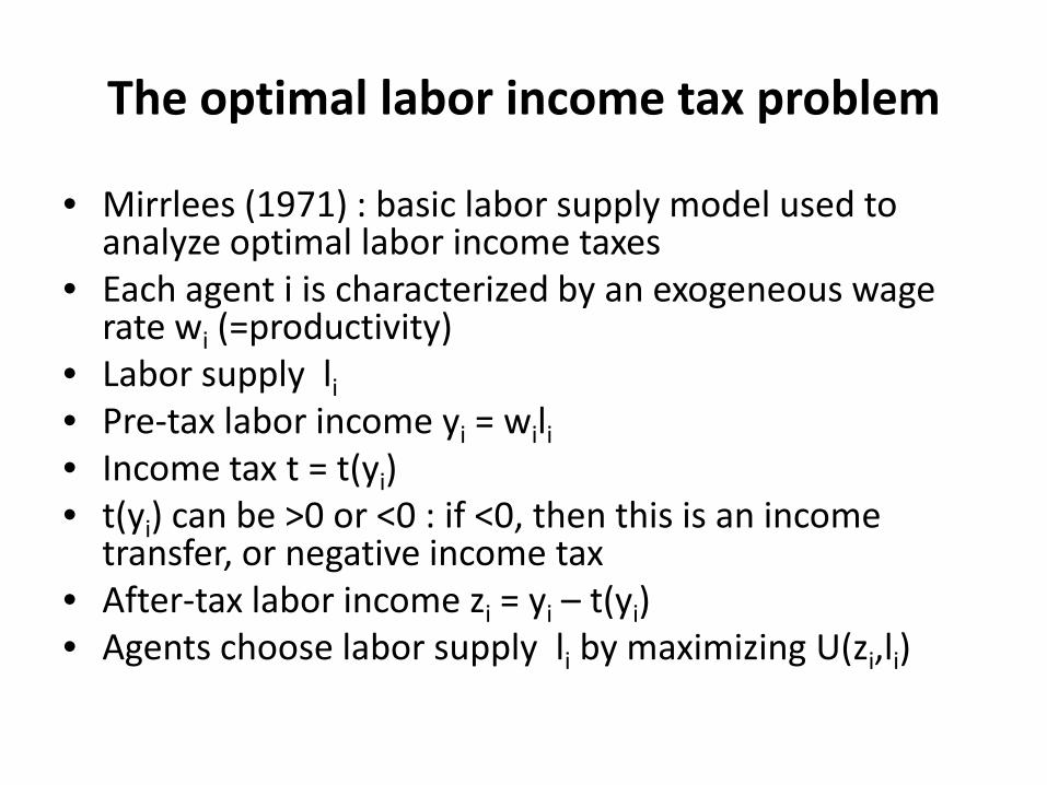
• Mirrlees (1971) : basic labor supply model used to analyze optimal labor income taxes

• Each agent i is characterized by an exogeneous wage rate wi (=productivity)

• Labor supply li • Pre-tax labor income yi = wili • Income tax t = t(yi) • t(yi) can be >0 or <0 : if <0, then this is an income

transfer, or negative income tax • After-tax labor income zi = yi – t(yi) • Agents choose labor supply li by maximizing U(zi,li)

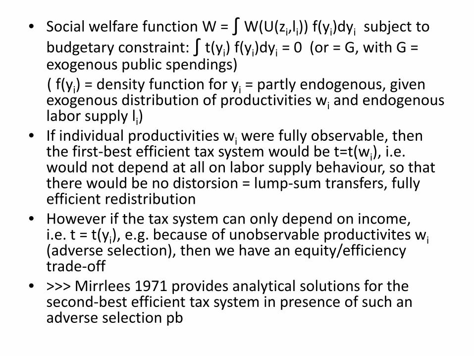
• Social welfare function W = ∫ W(U(zi,li)) f(yi)dyi subject to budgetary constraint: ∫ t(yi) f(yi)dyi = 0 (or = G, with G = exogenous public spendings)

( f(yi) = density function for yi = partly endogenous, given exogenous distribution of productivities wi and endogenous labor supply li)

• If individual productivities wi were fully observable, then the first-best efficient tax system would be t=t(wi), i.e. would not depend at all on labor supply behaviour, so that there would be no distorsion = lump-sum transfers, fully efficient redistribution

• However if the tax system can only depend on income, i.e. t = t(yi), e.g. because of unobservable productivites wi (adverse selection), then we have an equity/efficiency trade-off

• >>> Mirrlees 1971 provides analytical solutions for the second-best efficient tax system in presence of such an adverse selection pb

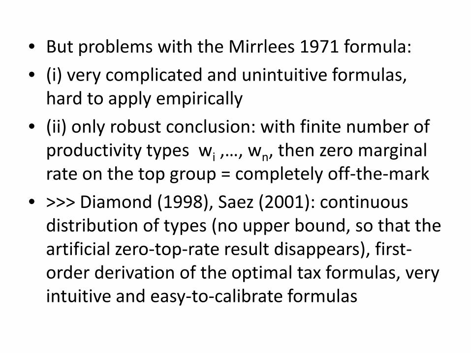
• But problems with the Mirrlees 1971 formula: • (i) very complicated and unintuitive formulas,

hard to apply empirically • (ii) only robust conclusion: with finite number of

productivity types wi ,…, wn, then zero marginal rate on the top group = completely off-the-mark

• >>> Diamond (1998), Saez (2001): continuous distribution of types (no upper bound, so that the artificial zero-top-rate result disappears), first-order derivation of the optimal tax formulas, very intuitive and easy-to-calibrate formulas

First-order derivation of linear optimal labor income tax formulas

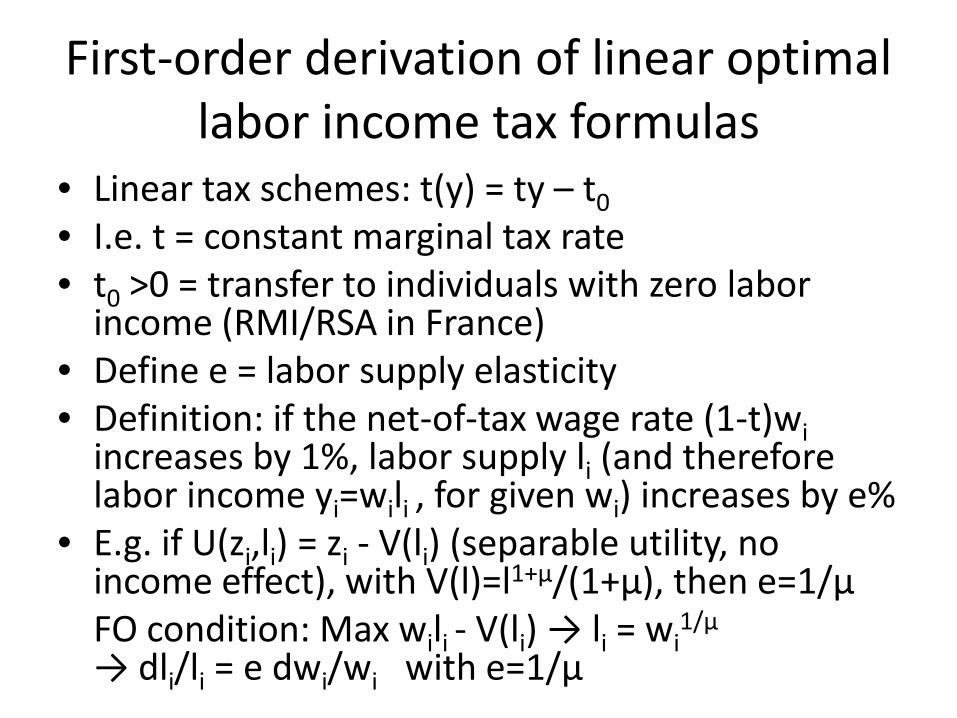
• Linear tax schemes: t(y) = ty – t0 • I.e. t = constant marginal tax rate • t0 >0 = transfer to individuals with zero labor

income (RMI/RSA in France) • Define e = labor supply elasticity • Definition: if the net-of-tax wage rate (1-t)wi

increases by 1%, labor supply li (and therefore labor income yi=wili , for given wi) increases by e%

• E.g. if U(zi,li) = zi - V(li) (separable utility, no income effect), with V(l)=l1+µ/(1+µ), then e=1/µ

FO condition: Max wili - V(li) → li = wi1/µ

→ dli/li = e dwi/wi with e=1/µ

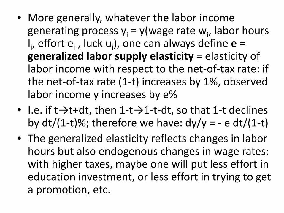
• More generally, whatever the labor income generating process yi = y(wage rate wi, labor hours li, effort ei , luck ui), one can always define e = generalized labor supply elasticity = elasticity of labor income with respect to the net-of-tax rate: if the net-of-tax rate (1-t) increases by 1%, observed labor income y increases by e%

• I.e. if t→t+dt, then 1-t→1-t-dt, so that 1-t declines by dt/(1-t)%; therefore we have: dy/y = - e dt/(1-t)

• The generalized elasticity reflects changes in labor hours but also endogenous changes in wage rates: with higher taxes, maybe one will put less effort in education investment, or less effort in trying to get a promotion, etc.

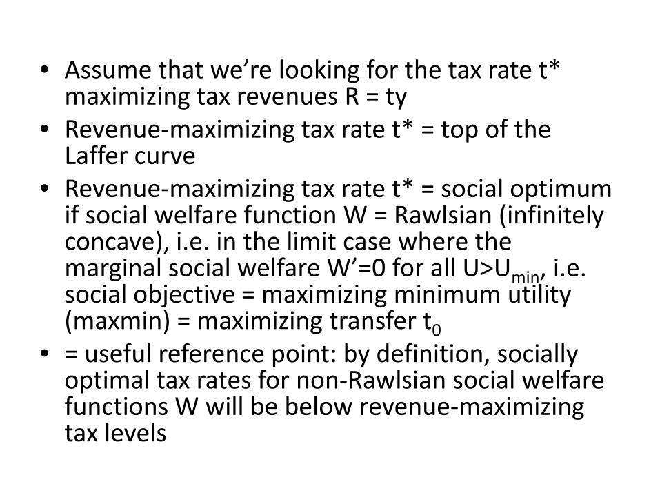
• Assume that we’re looking for the tax rate t* maximizing tax revenues R = ty

• Revenue-maximizing tax rate t* = top of the Laffer curve

• Revenue-maximizing tax rate t* = social optimum if social welfare function W = Rawlsian (infinitely concave), i.e. in the limit case where the marginal social welfare W’=0 for all U>Umin, i.e. social objective = maximizing minimum utility (maxmin) = maximizing transfer t0

• = useful reference point: by definition, socially optimal tax rates for non-Rawlsian social welfare functions W will be below revenue-maximizing tax levels

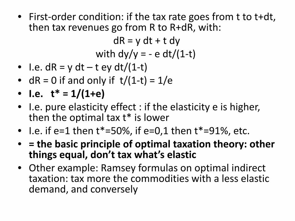
• First-order condition: if the tax rate goes from t to t+dt, then tax revenues go from R to R+dR, with:

dR = y dt + t dy with dy/y = - e dt/(1-t) • I.e. dR = y dt – t ey dt/(1-t) • dR = 0 if and only if t/(1-t) = 1/e • I.e. t* = 1/(1+e) • I.e. pure elasticity effect : if the elasticity e is higher,

then the optimal tax t* is lower • I.e. if e=1 then t*=50%, if e=0,1 then t*=91%, etc. • = the basic principle of optimal taxation theory: other

things equal, don’t tax what’s elastic • Other example: Ramsey formulas on optimal indirect

taxation: tax more the commodities with a less elastic demand, and conversely

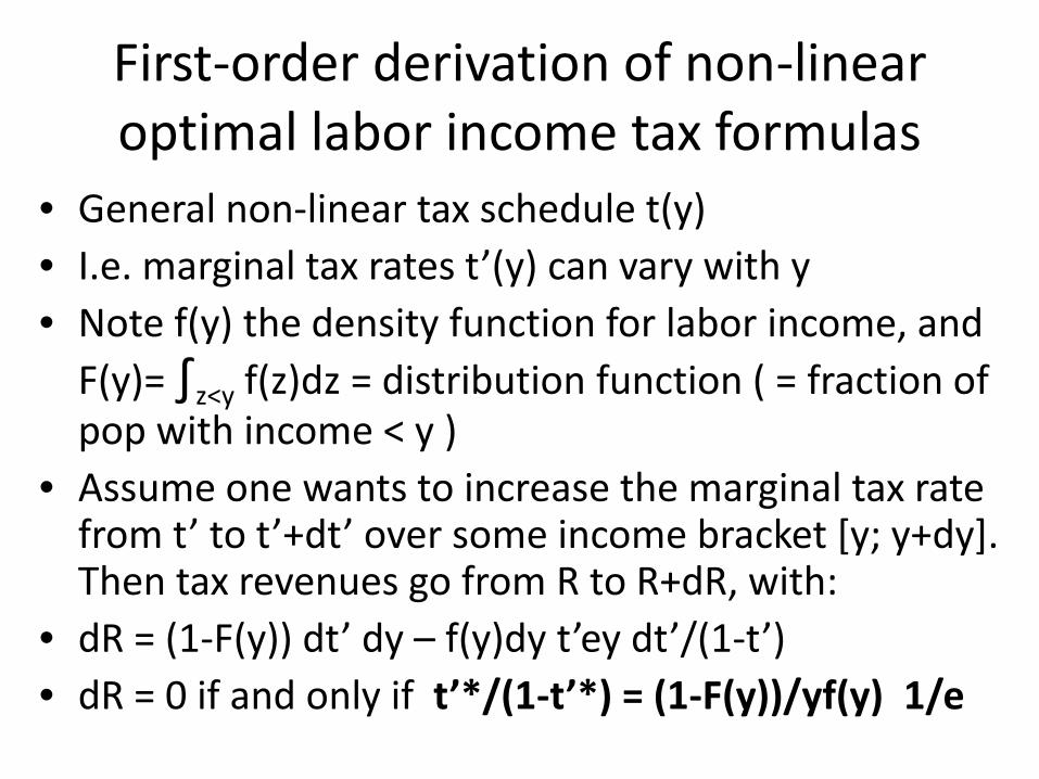
First-order derivation of non-linear optimal labor income tax formulas

• General non-linear tax schedule t(y) • I.e. marginal tax rates t’(y) can vary with y • Note f(y) the density function for labor income, and

F(y)= ∫z<y f(z)dz = distribution function ( = fraction of pop with income < y )

• Assume one wants to increase the marginal tax rate from t’ to t’+dt’ over some income bracket [y; y+dy]. Then tax revenues go from R to R+dR, with:

• dR = (1-F(y)) dt’ dy – f(y)dy t’ey dt’/(1-t’) • dR = 0 if and only if t’*/(1-t’*) = (1-F(y))/yf(y) 1/e

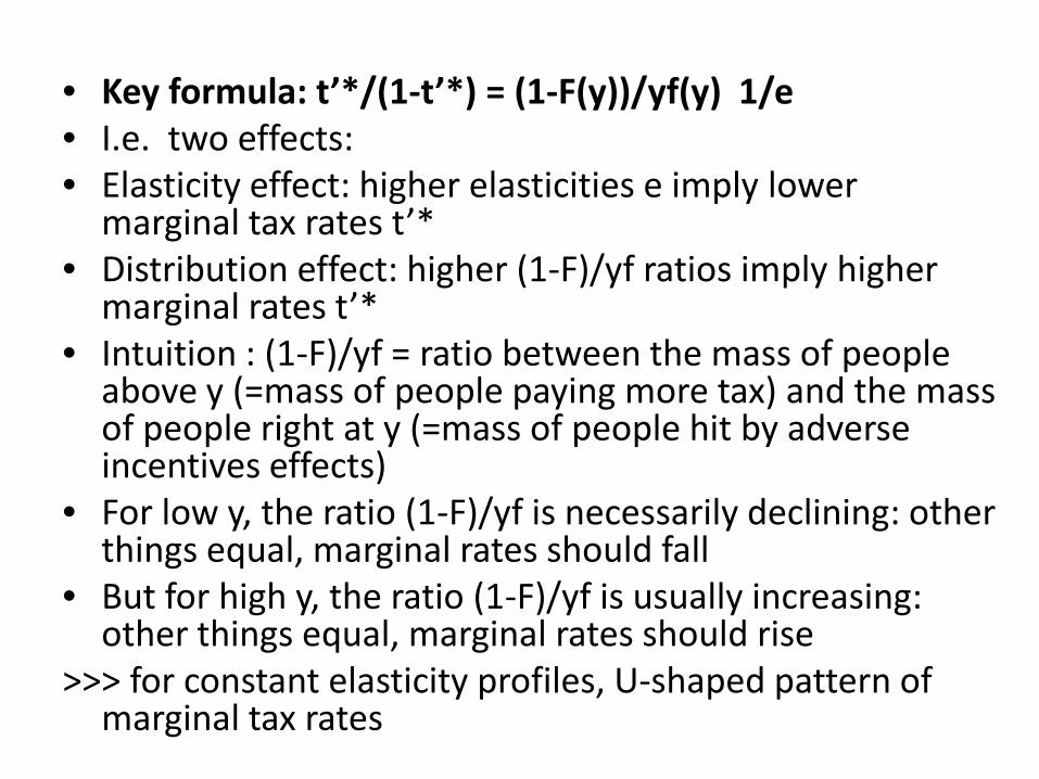
• Key formula: t’*/(1-t’*) = (1-F(y))/yf(y) 1/e • I.e. two effects: • Elasticity effect: higher elasticities e imply lower

marginal tax rates t’* • Distribution effect: higher (1-F)/yf ratios imply higher

marginal rates t’* • Intuition : (1-F)/yf = ratio between the mass of people

above y (=mass of people paying more tax) and the mass of people right at y (=mass of people hit by adverse incentives effects)

• For low y, the ratio (1-F)/yf is necessarily declining: other things equal, marginal rates should fall

• But for high y, the ratio (1-F)/yf is usually increasing: other things equal, marginal rates should rise

>>> for constant elasticity profiles, U-shaped pattern of marginal tax rates

Asymptotic optimal marginal rates for top incomes

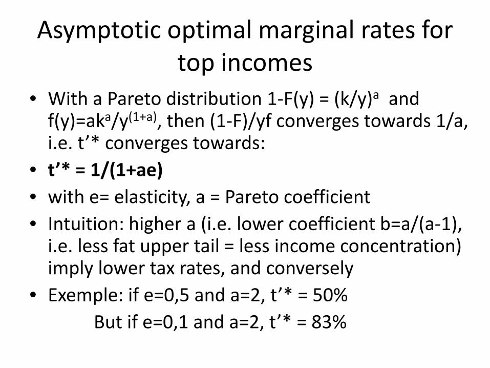
• With a Pareto distribution 1-F(y) = (k/y)a and f(y)=aka/y(1+a), then (1-F)/yf converges towards 1/a, i.e. t’* converges towards:

• t’* = 1/(1+ae) • with e= elasticity, a = Pareto coefficient • Intuition: higher a (i.e. lower coefficient b=a/(a-1),

i.e. less fat upper tail = less income concentration) imply lower tax rates, and conversely

• Exemple: if e=0,5 and a=2, t’* = 50% But if e=0,1 and a=2, t’* = 83%

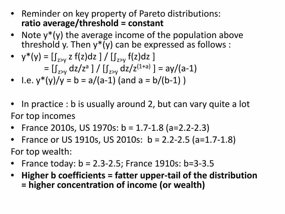
• Reminder on key property of Pareto distributions: ratio average/threshold = constant

• Note y*(y) the average income of the population above threshold y. Then y*(y) can be expressed as follows :

• y*(y) = [∫z>y z f(z)dz ] / [∫z>y f(z)dz ] = [∫z>y dz/za ] / [∫z>y dz/z(1+a) ] = ay/(a-1) • I.e. y*(y)/y = b = a/(a-1) (and a = b/(b-1) ) • In practice : b is usually around 2, but can vary quite a lot For top incomes • France 2010s, US 1970s: b = 1.7-1.8 (a=2.2-2.3) • France or US 1910s, US 2010s: b = 2.2-2.5 (a=1.7-1.8) For top wealth: • France today: b = 2.3-2.5; France 1910s: b=3-3.5 • Higher b coefficients = fatter upper-tail of the distribution

= higher concentration of income (or wealth)

Evidence on U-shaped pattern of marginal rates

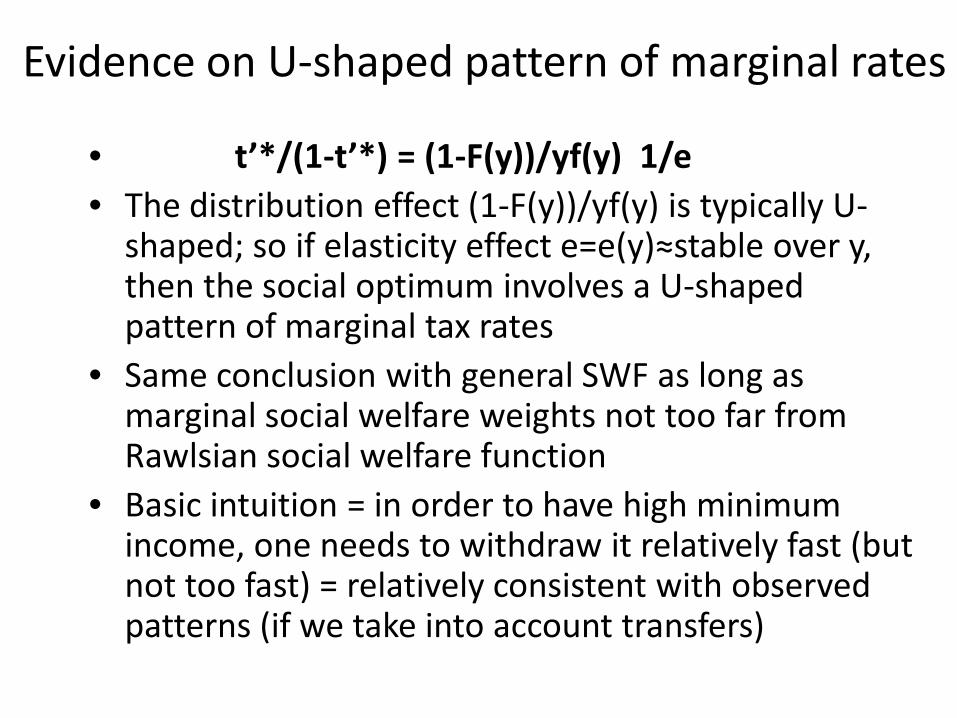
• t’*/(1-t’*) = (1-F(y))/yf(y) 1/e • The distribution effect (1-F(y))/yf(y) is typically U-

shaped; so if elasticity effect e=e(y)≈stable over y, then the social optimum involves a U-shaped pattern of marginal tax rates

• Same conclusion with general SWF as long as marginal social welfare weights not too far from Rawlsian social welfare function

• Basic intuition = in order to have high minimum income, one needs to withdraw it relatively fast (but not too fast) = relatively consistent with observed patterns (if we take into account transfers)

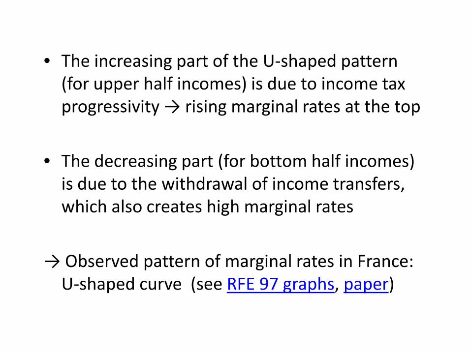
• The increasing part of the U-shaped pattern (for upper half incomes) is due to income tax progressivity → rising marginal rates at the top

• The decreasing part (for bottom half incomes)

is due to the withdrawal of income transfers, which also creates high marginal rates

→ Observed pattern of marginal rates in France:

U-shaped curve (see RFE 97 graphs, paper)

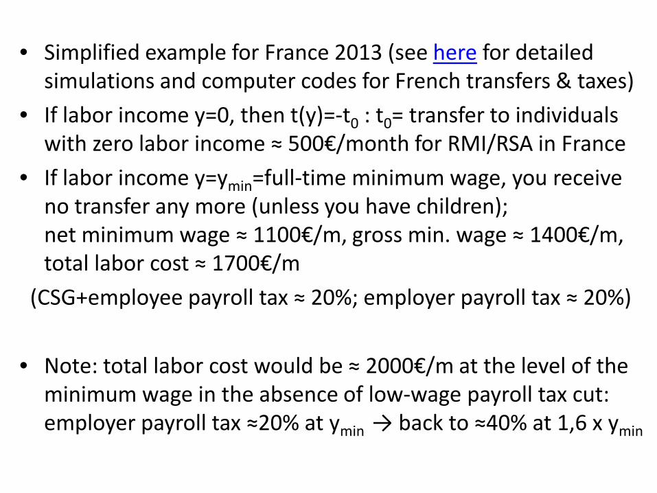
• Simplified example for France 2013 (see here for detailed simulations and computer codes for French transfers & taxes)

• If labor income y=0, then t(y)=-t0 : t0= transfer to individuals with zero labor income ≈ 500€/month for RMI/RSA in France

• If labor income y=ymin=full-time minimum wage, you receive no transfer any more (unless you have children); net minimum wage ≈ 1100€/m, gross min. wage ≈ 1400€/m, total labor cost ≈ 1700€/m

(CSG+employee payroll tax ≈ 20%; employer payroll tax ≈ 20%) • Note: total labor cost would be ≈ 2000€/m at the level of the

minimum wage in the absence of low-wage payroll tax cut: employer payroll tax ≈20% at ymin → back to ≈40% at 1,6 x ymin

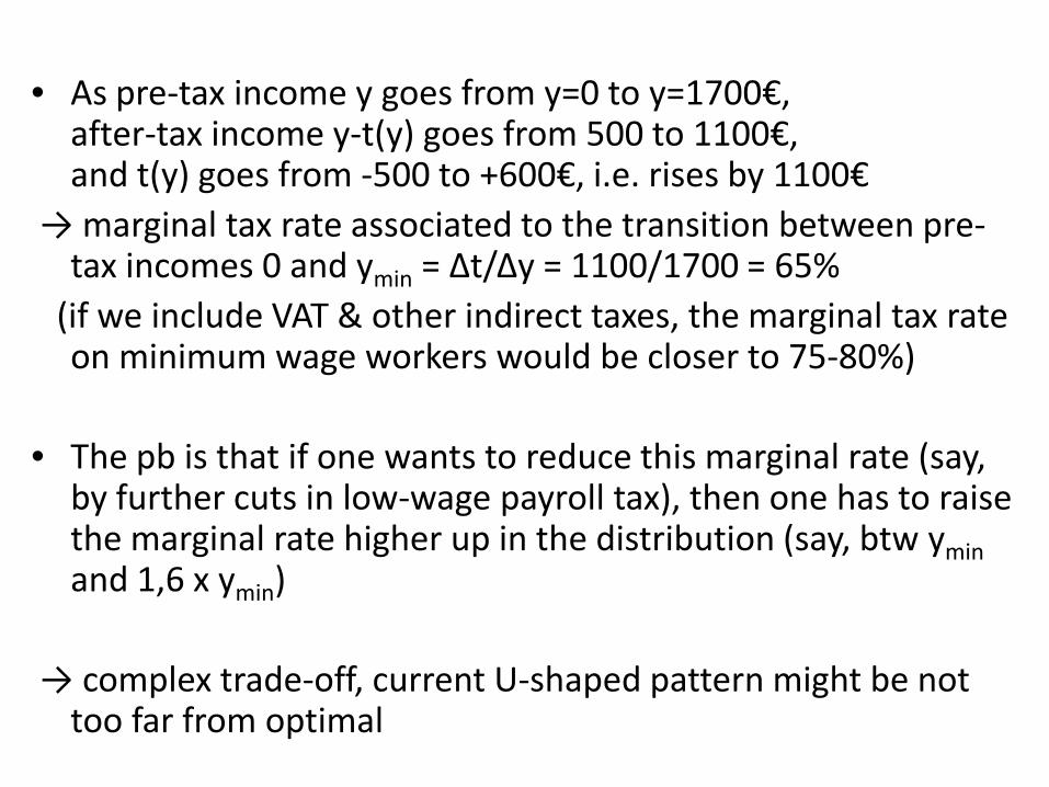
• As pre-tax income y goes from y=0 to y=1700€,

after-tax income y-t(y) goes from 500 to 1100€, and t(y) goes from -500 to +600€, i.e. rises by 1100€

→ marginal tax rate associated to the transition between pre-tax incomes 0 and ymin = Δt/Δy = 1100/1700 = 65%

(if we include VAT & other indirect taxes, the marginal tax rate on minimum wage workers would be closer to 75-80%)

• The pb is that if one wants to reduce this marginal rate (say,

by further cuts in low-wage payroll tax), then one has to raise the marginal rate higher up in the distribution (say, btw ymin and 1,6 x ymin)

→ complex trade-off, current U-shaped pattern might be not too far from optimal

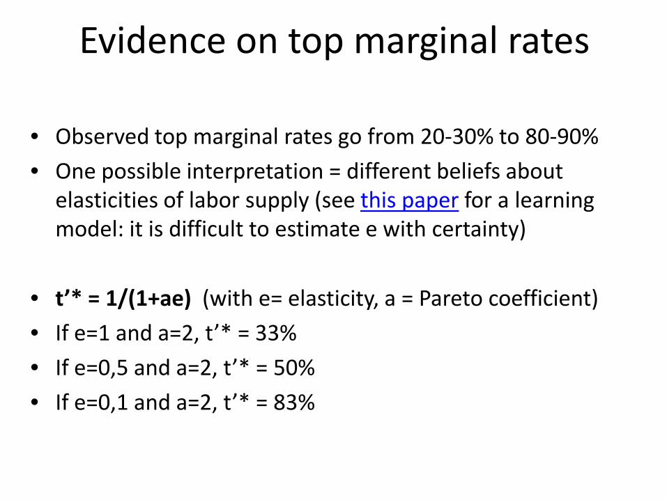
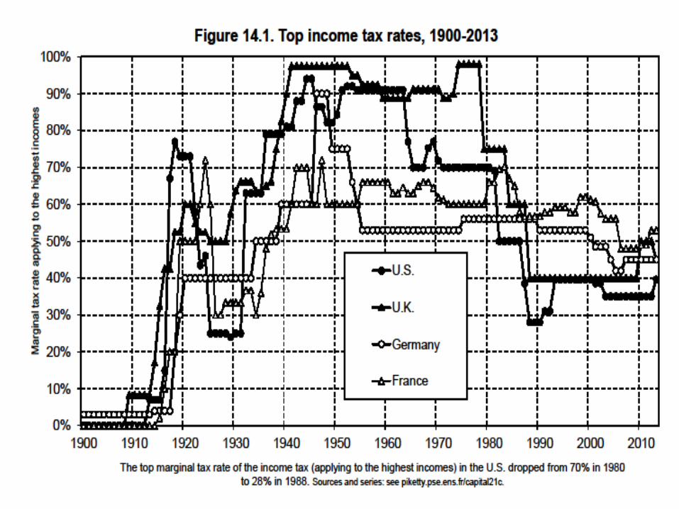
Evidence on top marginal rates • Observed top marginal rates go from 20-30% to 80-90% • One possible interpretation = different beliefs about

elasticities of labor supply (see this paper for a learning model: it is difficult to estimate e with certainty)

• t’* = 1/(1+ae) (with e= elasticity, a = Pareto coefficient) • If e=1 and a=2, t’* = 33% • If e=0,5 and a=2, t’* = 50% • If e=0,1 and a=2, t’* = 83%

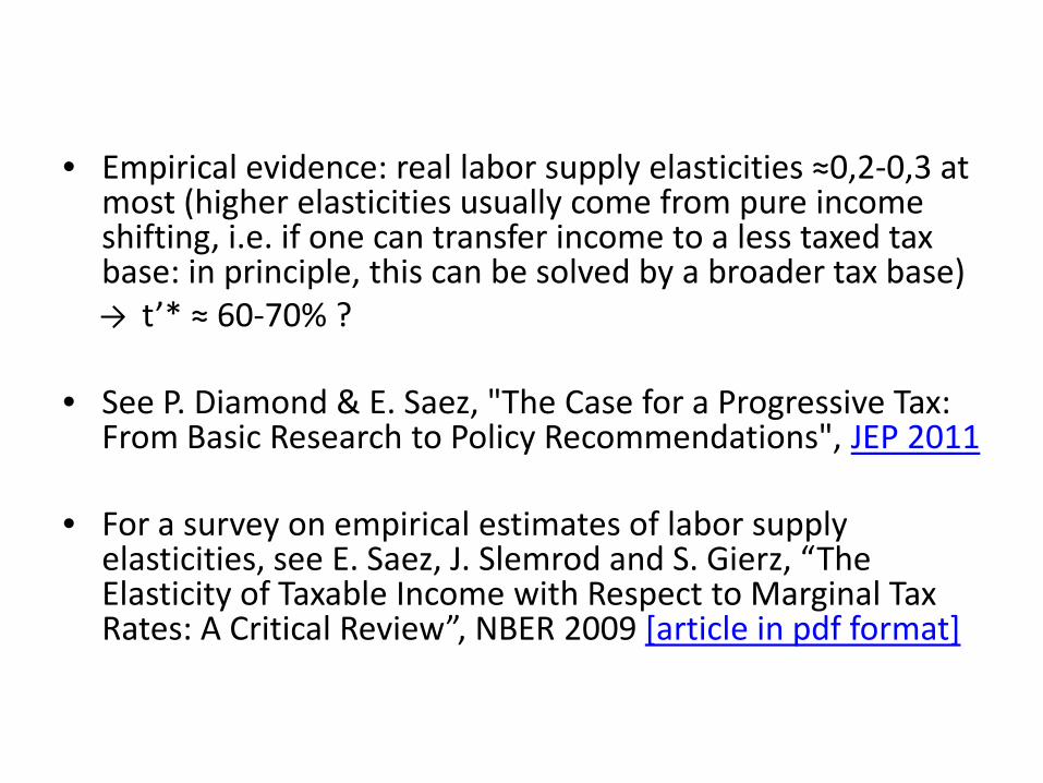
• Empirical evidence: real labor supply elasticities ≈0,2-0,3 at

most (higher elasticities usually come from pure income shifting, i.e. if one can transfer income to a less taxed tax base: in principle, this can be solved by a broader tax base)

→ t’* ≈ 60-70% ? • See P. Diamond & E. Saez, "The Case for a Progressive Tax:

From Basic Research to Policy Recommendations", JEP 2011

• For a survey on empirical estimates of labor supply elasticities, see E. Saez, J. Slemrod and S. Gierz, “The Elasticity of Taxable Income with Respect to Marginal Tax Rates: A Critical Review”, NBER 2009 [article in pdf format]

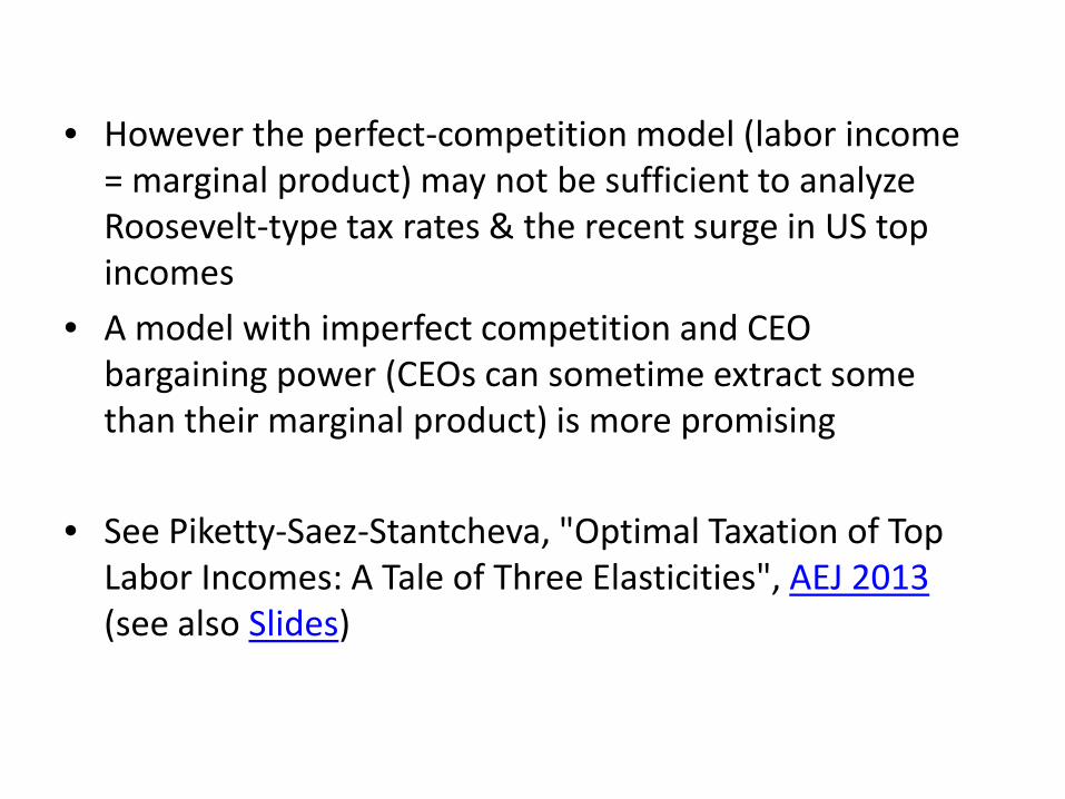
• However the perfect-competition model (labor income

= marginal product) may not be sufficient to analyze Roosevelt-type tax rates & the recent surge in US top incomes

• A model with imperfect competition and CEO bargaining power (CEOs can sometime extract some than their marginal product) is more promising

• See Piketty-Saez-Stantcheva, "Optimal Taxation of Top

Labor Incomes: A Tale of Three Elasticities", AEJ 2013 (see also Slides)

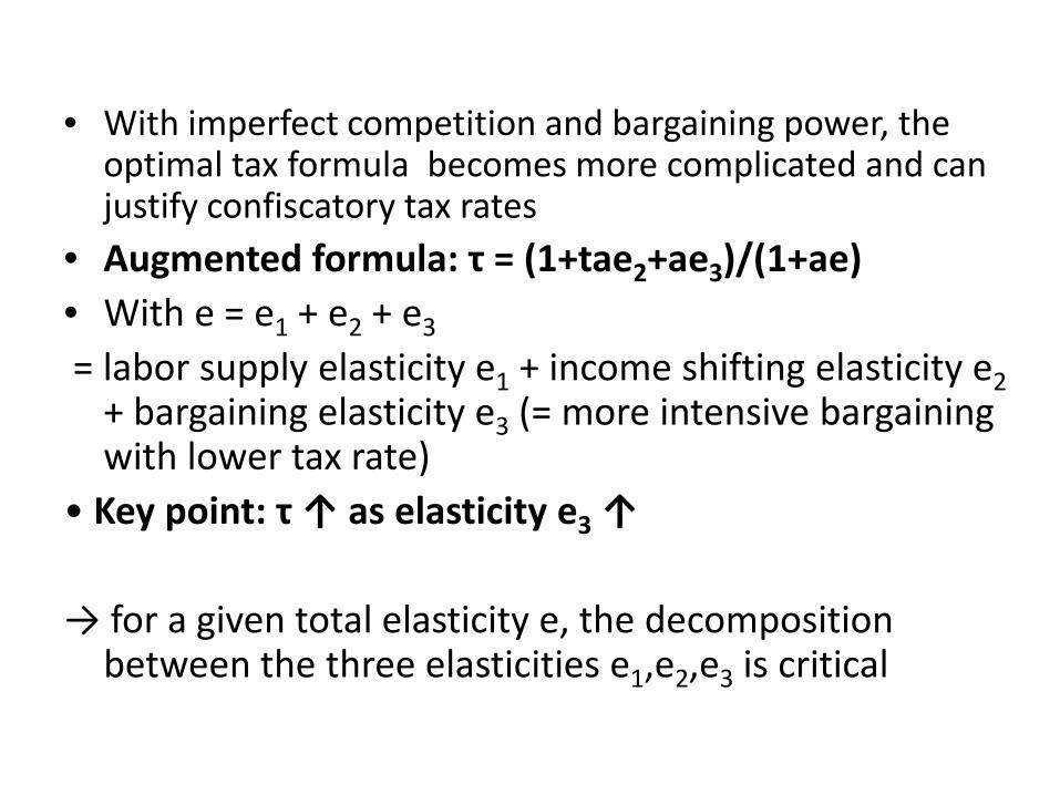
• With imperfect competition and bargaining power, the

optimal tax formula becomes more complicated and can justify confiscatory tax rates

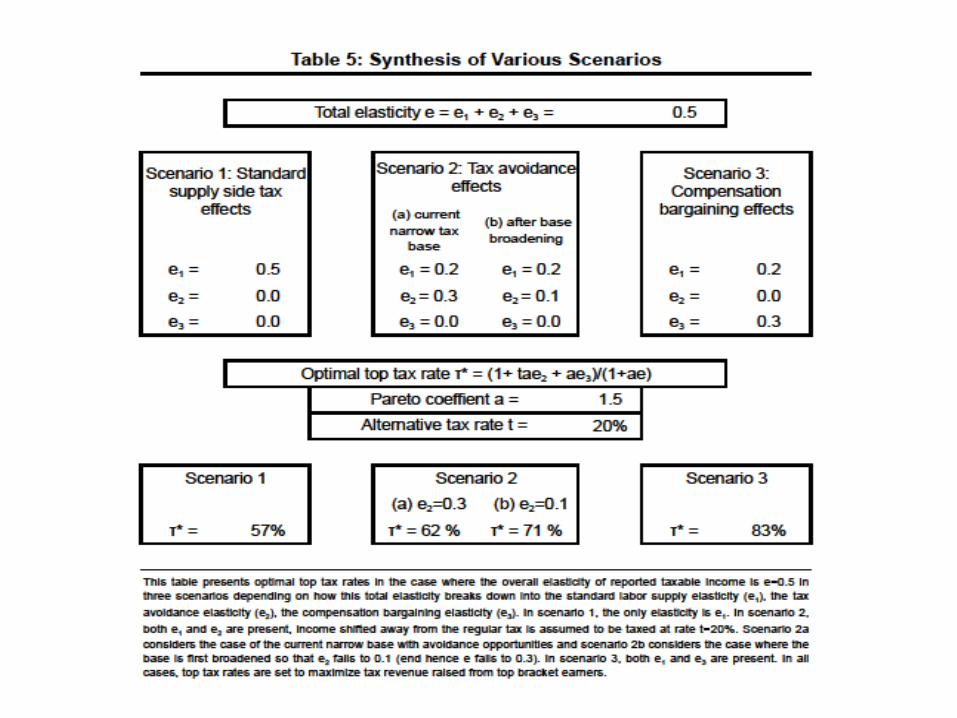
• Augmented formula: τ = (1+tae2+ae3)/(1+ae) • With e = e1 + e2 + e3 = labor supply elasticity e1 + income shifting elasticity e2

+ bargaining elasticity e3 (= more intensive bargaining with lower tax rate)

• Key point: τ ↑ as elasticity e3 ↑ → for a given total elasticity e, the decomposition

between the three elasticities e1,e2,e3 is critical