Public Investment, Growth, and Debt Sustainability: Putting Together the Pieces

Edward E. Buffie, Andrew Berg, Catherine Pattillo,

Rafael Portillo, and Luis-Felipe Zanna

WP/12/144

© 2012 International Monetary Fund WP/12/144 IMF Working Paper Research Department

Public Investment, Growth and Debt Sustainability: Putting Together the Pieces Prepared by Edward Buffie, Andrew Berg, Catherine Pattillo, Rafael Portillo, and Luis-Felipe Zanna1

June 2012

Abstract

This Working Paper should not be reported as representing the views of the IMF. The views expressed in this Working Paper are those of the author(s) and do not necessarily represent those of the IMF or IMF policy, or of DFID. Working Papers describe research in progress by the author(s) and are published to elicit comments and to further debate.

We develop a model to study the macroeconomic effects of public investment surges in low-income countries, making explicit: (i) the investment-growth linkages; (ii) public external and domestic debt accumulation; (iii) the fiscal policy reactions necessary to ensure debt-sustainability; and (iv) the macroeconomic adjustment required to ensure internal and external balance. Well-executed high-yielding public investment programs can substantially raise output and consumption and be self-financing in the long run. However, even if the long run looks good, transition problems can be formidable when concessional financing does not cover the full cost of the investment program. Covering the resulting gap with tax increases or spending cuts requires sharp macroeconomic adjustments, crowding out private investment and consumption and delaying the growth benefits of public investment. Covering the gap with domestic borrowing market is not helpful either: higher domestic rates increase the financing challenge and private investment and consumption are still crowded out. Supplementing with external commercial borrowing, on the other hand, can smooth these difficult adjustments, reconciling the scaling up with feasibility constraints on increases in tax rates. But the strategy may be also risky. With poor execution, sluggish fiscal policy reactions, or persistent negative exogenous shocks, this strategy can easily lead to unsustainable public debt dynamics. Front-loaded investment programs and weak structural conditions (such as low returns to public capital and poor execution of investments) make the fiscal adjustment more challenging and the risks greater. JEL Classification Numbers: E62, F34, H63, O43, H54. Keywords: Public Investment, Growth, Debt Sustainability, Fiscal Policy, Infrastructure, Aid

Mail Author’s E-Addresses:

ebuffie@indiana.edu; aberg@imf.org; cpattillo@imf.org; rportillo@imf.org; fzanna@imf.org

1 We thank Valerio Crispolti, Raphael Espinoza, Giovanni Ganelli, Andrew Jewell, Alvar Kangur, Chris Papageorgiou, Jens Reinke, Carlo Sdralevich, Susan Yang, and participants of the MMDG seminar of the African department at the IMF, the 2011 AERC/UNU-WIDER Macroeconomics of Foreign Aid Meeting, and the 2012 CSAE conference in Oxford for useful comments. All errors remain ours. This working paper is part of a research project on macroeconomic policy in low-income countries supported by the U.K.'s Department for International Development (DFID). Edward Buffie: Department of Economics, Indiana University, Wylie Hall Rm 105, 100 S. Woodlawn, Bloomington, IN 47405.

2

Table of Contents Page

I. Introduction ..........................................................................................................................4 II. The Model ............................................................................................................................9 A. Firms ...............................................................................................................................9 A.1. Technology.............................................................................................................9 A.2. Factor Demands ...................................................................................................10 B. Consumers .....................................................................................................................11 C. The Government ............................................................................................................13 C.1. Infrastructure, Public Investment and Efficiency .................................................13 C.2. Fiscal Adjustment and the Public Sector Budget Constraint ...............................14 D. Market-Clearing Conditions and External Debt Accumulation ....................................17 III. Calibration of the Model ....................................................................................................17 IV. The Long-Run Outcome ....................................................................................................23 A. Insights from a Simplified Model .................................................................................24 B. Numerical Solutions ......................................................................................................26 V. The Medium-Term Fiscal and Macroeconomic Adjustments under Different Financing

Schemes .............................................................................................................................28 A. Unconstrained Tax Adjustment ....................................................................................28 A.1. The Base Case ......................................................................................................28 A.2. More Optimistic and Troublesome Scenarios ......................................................30 A.3. Gradually Increasing Transfers, Efficiency, and the Collection Rate of User Fees ......................................................................................................................32 B. Constrained Tax Adjustment Combined with External Commercial Borrowing .........36 B.1. Tax Smoothing and Private Demand Crowding Out ...........................................36 B.2. Debt Blowups: Structural and Policy Conditions ................................................38 C. Constrained Tax Adjustment Combined with Domestic Borrowing ............................39 VI. External Shocks and Risks .................................................................................................41 VII. Concluding Remarks ........................................................................................................44 Tables Table 1. Base Case Calibration ................................................................................................19 Table 2. Public Investment Scaling Up, Concessional Borrowing, and Grants .....................23 Table 3. Long-run Effects of Scaling up Public Investment by 3 Percent of Initial GDP .......27 Figures Figure 1. The Long-run Outcome in the Simplified Model .....................................................24 Figure 2. Base Case: Unconstrained Tax Adjustment .............................................................29 Figure 3. Unconstrained Tax Adjustment: Optimistic and Troublesome Scenarios ...............31

3

Figure 4. Unconstrained Tax Adjustment: The Size of the Scaling Up ...................................33 Figure 5. Unconstrained Tax Adjustment: Increasing Transfers .............................................34 Figure 6. Unconstrained Tax Adjustment versus Constrained Tax Adjustment with External Commercial Borrowing .............................................................................37 Figure 7. Constrained Tax Adjustment with External Commercial Borrowing: Varying the Structural and Policy Conditions .......................................................................38 Figure 8. Constrained Tax Adjustment: Domestic Borrowing versus External Commercial Borrowing ...............................................................................................................40 Figure 9. External TOT Shocks: Shocks Persistence and Financing Schemes ........................41 Figure 10. TFP and Risk Premium Shocks and Risks .............................................................43 Appendix A. On Public Investment Efficiency, Rates of Return, and Growth ........................................46 References ...............................................................................................................................49

4

I. Introduction

Many low-income countries (LICs) are facing dire infrastructure gaps.1 For the first time in

decades, many also have substantial growth momentum, low debt levels, and access to nonconcessional

foreign credit. Meanwhile, aid resources are not increasing as promised.2 The opportunity to borrow

nonconcessionally to meet infrastructure needs has thus become very tempting.3

The risks associated with excessive borrowing to finance these public investment plans need to be

considered as well. The Highly Indebted Poor Country (HIPC) and Multilateral Debt Relief initiatives

(MDRI) reduced the external debt of the poorest countries by ninety percent over the past decade.

This followed decades of struggle by these countries to work their way out from onerous debt levels,

which were mostly accumulated in the 1970s, the last time many of them were growing rapidly and

had access to new foreign lending on a large scale. Debt indicators in LICs are still far below the

levels seen in the mid-90s. However, rapid accumulation of new debt in these countries–especially

the increasing reliance on more expensive domestic and external commercial debt–could bring back

the spectre of debt crisis, macroeconomic instability, and severely impaired development prospects.4

The IMF and World Bank (IMF-WB) use a debt sustainability framework (DSF) to identify

overborrowing situations that may endanger macroeconomic stability. In the DSF, a baseline set

of 20-year projections for borrowing, GDP growth, exports, and other key macroeconomic variables

underpin an analysis of key debt ratios. In this debt sustainability analysis (DSA), a country is at

“high risk” of debt distress if any of the debt ratios–such as debt/GDP and debt/exports–exceed a

specified threshold in the baseline scenario over the 20-year horizon. The thresholds in turn have been

determined based on empirical evidence linking these ratios to subsequent episodes of debt distress.5 A

country is at “moderate risk” if the ratios exceed the thresholds in one of several specified alternative

scenarios or “stress tests” that simulate negative growth shocks and nominal exchange rate shocks,

among others.6 But, of course, judgement is used by staff when assigning risk ratings.

The DSF has helped countries monitor their risk of debt distress and sharpened the IMF-WB’s

assessments and policy advice, but it has been also subject to several criticisms.

1See Foster and Briceño-Garmendia (2010).2For example, Redifer (2010) points out that the four East African countries with new Fund’s Policy Support Instru-

ment Programs (Mozambique, Rwanda, Tanzania, and Uganda), official aid has on average not increased in line with

public investment spending and is not projected to do so in the next three years; therefore new financing sources, such

as external commercial borrowing, must be tapped if public investment is to be scaled up.3A recent survey by Citigroup describes the new borrowing environment: “Knowing they want to borrow money to

spend on projects to close the infrastructure deficit, governments in SSA have faced a wave of lenders looking to get

money out of the door and into their pockets: whether investment bankers extolling the virtues of issuing Eurobonds;

apparently cheap BRIC country loans, but with long-term catches on payment implications . . .” (Cowan, 2010, p.9). A

call to borrow for development neeeds is endorsed by UNCTAD (2004) and EURODAD (2001, 2009), in the context of

the human development approach to debt sustainability.4See IMF and World Bank (2006) and Barkbu et al. (2008), among others.5The thresholds depend on the quality of policies and institutes as measured by the Country Policy and Institutional

Assessment (CPIA) index of the World Bank.6See IMF(2010) for the most recent guidelines on the application of the DSF to LICs.

5

One of the criticisms is that the DSF does not contain a consistent analytic framework for creat-

ing the 20-year projections. Sachs (2002), for instance, argues that “the so-called debt sustainability

analysis is built on the flimsiest of foundations,” arguing that it is little more than a set of accounting

identities and exogenous projections. In the same vein, Eaton (2002) and Hjertholm’s (2003) have

raised concerns that IMF-WB’s debt projections are not derived from an integrated, internally con-

sistent macroeconomic framework. A specific aspect of this criticism is that the IMF-WB projections

do not take sufficiently into account the relationship between public investment and growth. That

is, the projections generally do not make an explicit linkage between the public investment that the

proposed nonconcessional borrowing is meant to finance and the resulting growth that should make

the operation self-financing. This inflates debt indicators, such as debt-to-GDP ratios, creates a bias

toward conservative borrowing limits, and can amount “to sacrificing growth to imprecisely known

debt sustainability risks” (Wyplosz, 2007).

Another concern relates to the treatment of fiscal policy in the forward-looking framework. The

DSF concept of solvency requires that debt stay below the thresholds absent a “major correction” in

policies. It cannot, in the view of Wyplosz (2007), be invoked to argue that a particular level of debt,

or even a prolonged rising path, signifies debt distress. After all, even a very good project may take

some time to pay off, and in the interim the debt ratios may exceed a given threshold. Moreover, the

stress tests assume that the government does not react to shocks, contradicting evidence that primary

balances in fact respond to rising public debt and potentially making the tests too conservative.7

This paper addresses these criticisms by proposing an internally consistent quantitative macroeco-

nomic framework that may be useful in constructing the scenarios necessary for debt sustainability

analysis. The model has many LIC-specific components, but it is centered on the public investment-

growth nexus.8 In the end, judgement will be critical in making projections and scenarios for the DSF,

whether through purely ad hoc forecasts or the careful calibration of the model. But the model should

serve to: make explicit the assumptions underlying the projections, furthering discussions internally

and with stakeholders based on different simulated scenarios; help apply empirical information, for

example on project rates of return; and allow more systematic risk assessments.

In putting the model through its paces to analyze debt-led public investment scaling ups in a typical

Sub-Saharan African (SSA) LIC, the paper demonstrates the importance of a coherent forward-looking

analysis, with explicit policy reaction functions that may respond to debt levels. An overarching

conclusion regarding the debt sustainability impact of ambitious public investment plans is that it is

not enough to compare the rate of return of these plans to their cost of funding.9 Rather, the absorptive

capacity of the country, the efficiency of public investment spending, the response of the private sector,

7For this evidence see Celasun et al. (2007), among others. In the current review of the DSF, Fund and World

Bank staff are proposing the inclusion, on an optional basis, of a new stress test reflecting dynamic linkages between

macroeconomic variables.8The Fund acknowledges the need for strengthening analysis of the investment/growth nexus in DSAs, including

through development and operationalizing models to provide a consistent way to assess the complex interlinkages (IMF

and World Bank, 2009).9Thus we disagree with Wyplosz (2007): “If external borrowing is growth enhancing, the risk of over borrowing is

small, possibly inexistent. If, instead, external borrowing does not exert any favorable growth effect, and possibly stunts

growth, DSA is moot . . . (p.14)”.

6

the authorities’ ability to adjust taxes and spending, and other factors shape the benefits–and the

debt sustainability risks–of these investment plans.

A further criticism is that the DSF-based debt limits policy is not flexible enough in allowing

countries with IMF-supported programs to borrow nonconcessionally. In response, the IMF has re-

cently made its policies more flexible.10 The question of how to move from an analysis of debt

sustainability to the application of borrowing limits in IMF-supported programs is outside the scope

of this paper. Rather, the sole focus here is on the macroeconomic framework–the projections and

scenarios–underlying the DSF. However, we hope that the availability of more coherent medium-term

framework, incorporating public investment/growth linkages, will allow better analysis and application

of borrowing limits in difficult cases.11

With these goals in mind, we construct an optimizing intertemporal model that embeds features

that seem crucial to capturing the main mechanisms and policy issues of interest for DSAs in LICs.

The model incorporates a neoclassical production function with private and public capital. Because

public capital is productive, government spending can raise output directly and crowd in as well as

crowd out private investment. The parameters of the production function determine the rate of return

to installed public capital.

Several distinct features capture aspects of the challenges LIC governments have faced historically

in making productive public investments. First, spending on public investment does not always imply

an equivalent increase in the stock of public capital. Depending on the “efficiency” of public investment,

some of the spending may be wasted or spent on poor (inframarginal) projects. In addition, we assume

an “absorptive capacity” problem: due to coordination problems or supply bottlenecks during the

implementation phase of public investment projects, unusually high investment rates may result in

large costs overruns that affect the budget. Both efficiency and absorptive capacity play key roles in

determining the final impact of public investment on growth, along with the rate of return to public

capital.12

We allow for different government financing options and state explicitly the fiscal policy reactions

that may ensure debt sustainability. In our analysis, we take available aid and concessional borrowing

flows as exogenously given. Absent additional financing sources, the government adjusts taxes and

transfers to finance the public investment scaling up. The model then considers external commercial

10The IMF has recently modified its policies on nonconcessional borrowing by LICs in the context of IMF-supported

programs to reflect better the diversity of LICs and their financing patterns, and offer more flexibility depending on

countries’ debt vulnerabilities and public financial management capacity. See IMF(2009b) for the guidelines on debt

limits in Fund-supported programs.11The IMF and World Bank Boards have stated that until the investment-growth nexus is incorporated concerns will

persist that “the DSF has unduly constrained the ability of LICs to finance their development goals.”See IMF and World

Bank (2009).12As in Berg et al. (2010b), we also introduce learning-by-doing externalities in the production of both sectors, defined

in terms of sectoral outputs. These externalities capture the Dutch-disease (Dutch-vigor) notion that real exchange

appreciation (depreciation) may harm (help) productivity growth in the traded sector, which is a major concern in LICs

that face aid surges, including substantial increases in concessional borrowing. Nevertheless, in this paper we do not

elaborate on the implications of these externalities for debt sustainability.

7

borrowing and domestic borrowing to help finance the public investment surge, with taxes and transfers

responding to stabilize debt levels over time. The model allows the imposition of feasibility constraints

on the pace or level of these fiscal adjustments for taxes and transfers, potentially yielding explosive

debt trajectories.

Finally, the model contains a number of other features and shocks that are common in LICs and

shape the macroeconomic effects of public investment surges. The model has traded and non-traded

sectors and separate prices for exports and imports. These features allow an analysis of the real ex-

change rate and the need to achieve external and internal balance; they also permit the analysis of

shocks to the terms of trade (TOT). On the private sector side, it incorporates hand-to-mouth con-

sumers and limited access to international capital markets to capture financial market imperfections.

The presence of these consumers helps break Ricardian equivalence. The limited access to international

capital markets is key to making nonconcessional borrowing by the government important. With fully

open capital accounts, it would not matter whether the government borrowed domestically or abroad,

for example, as private agents could borrow abroad to lend to the government. In addition to TOT

shocks, the model incorporates shocks to the government external debt risk premium (or world interest

rates) and negative total factor productivity (TFP) shocks, as a way to model natural disaster shocks.

Because the future is uncertain, asserting that a path of public debt is unsustainable is still chal-

lenging. As Wyplosz (2007) argues “it is future balances that matter, not the past and not just the

current debt level. Huge debts can be paid back, and small debts may not be sustainable, it all de-

pends on what the primary balance will look like in the future, including the very distant future.” Our

model provides a logically consistent framework that helps unveil the trade-offs and potential risks

associated with different types of financing and fiscal policy reactions. Given a calibration and some

assumptions about structural conditions, financing options and fiscal policy reactions of a particular

LIC, the model can help IMF country teams or country authorities build different scenarios to inform

the DSA. This should help articulate and dissect ambitious borrowing plans that aim to push growth

above historical averages along with analysis of “an alternative high-investment, low-growth payoff

scenario” to counterbalance potential tendencies toward excessive optimism.13

We calibrate the model to the “average” LIC and pursue different policy experiments, whose results

speak directly to many of the issues that have preoccupied the literature:

• Despite the low tax-take in LICs, increases in infrastructure investment may be self-financing inthe long run. The favorable long-run effect on the budget reflects extra increases in output and

revenue associated with strong crowding in of private capital. For this to happen the economy

must feature strong structural conditions, such as high returns on public capital, high public

investment efficiency and high collection rates of user fees, among others.

• Even very good (high rate-of-return) projects may not be fully self-financing, however, becausemost of the direct benefits of the higher public capital accrue to the private sector and average

tax collection rates are quite low.

13On calls to pursue alternative scenarios in DSAs, see IMF and World Bank (2006) and Barkbu et al. (2008).

8

• Even if the investment program is self-financing in the long run, transition problems can be

formidable. Absent additional borrowing or aid, the revenue gains from growth will not mate-

rialize soon enough to obviate the need for difficult fiscal adjustments on the transition path,

especially when the scaling up is front-loaded. Tax rates may have to increase sharply, crowding

out private investment and consumption and further aggravating the near-term fiscal challenge.

• Nonconcessional external borrowing can smooth away difficult fiscal adjustments, reconcilingscaling up of public investment with constraints on feasible increases in tax rates (or cuts in

spending). But this strategy may be risky. Low rates of return, inefficient public investment,

sluggish fiscal adjustment, or low absorptive capacity can easily lead to unsustainable public

debt.

• Borrowing in the domestic debt market is ineffective in smoothing the path of fiscal adjustmentand avoiding private sector crowding out. It does not provide additional resources from abroad, so

the public investment scaling up still requires a decline in private consumption and investment

in the first few years. In addition, interest rates are likely to be higher than with external

borrowing, which further deteriorates the prospects for private investment.

• Commercial borrowing can make the economy more vulnerable to macroeconomic instability inthe presence of persistent unexpected shocks, such as to the TOT, TFP, or public debt risk

premium. These shocks are less prone to ignite explosive paths of public debt when aid or

concessional lending responds positively to negative shocks.

• Because there is uncertainty about the underlying parameters and because of exogenous shocks,size matters. If the increase in public investment is small relative to the size of the economy,

then the risk of debt distress does not depend much on these parameters or on the shocks. But

as the investment grows larger, they become more critical to the risks of debt distress.

Our work distinguishes itself from the literature that studies the macroeconomic effects of public

investment by analyzing the trade-offs of different types of public debt, while underscoring the role

for debt sustainability of i) structural and policy conditions and ii) exogenous shocks. The seminal

works by Barro (1990), Sala-i-Martin (1992), Futagami et al. (1993) and Glomm and Ravikumar

(1994) analyze the growth impact of public investment in the context of endogenous growth models.

More recently, Chatterjee and Turnovsky (2007) and Agenor (2010), among others, have relied on

these endogenous growth setups to explore the importance of some LIC-specific features for the public

capital accumulation and growth nexus. The former explore the importance of tied vs untied aid, while

the latter emphasizes the role of infrastructure network effects and the efficiency of public investment.

All these models, however, assume government balanced budget rules, thereby abstracting from public

debt accumulation. On the other hand, Turnovsky (1999), Greiner et al. (2005) and Greiner (2007),

among others, incorporate government debt in their endogenous growth framework. In contrast to our

work, they do not allow for different financing schemes and ignore the role played by the structural

and policy conditions for debt sustainability. Finally, the works by Adam and Bevan (2006), Cerra et

al. (2008), and Berg et al. (2010b), among others, look into the macroeconomic effects of aid-financed

public investment expansions. But here again, external public debt accumulation is not allowed and,

therefore, the interaction of structural and policy conditions with debt dynamics is missing.

9

Finally, our paper is also related to the literature about debt sustainability, but our emphasis is

on LICs. Celasun et al. (2007), Garcia and Rigobon (2005), and Mendoza and Oviedo (2004), among

others, focus on emerging economies; while Bohn (1998) and Ghosh et al. (2011), among others,

concentrate on advanced economies.

The main body of the paper is organized into seven sections. In Sections II and III we explicate

the model and calibrate it to the “average” LIC. Following these, Section IV analyzes the long-run

impact of a permanent, large increase in public investment. Then Sections V and VI investigate the

medium-term trade-offs and potential risks associated with the different financing schemes. Finally,

Section VII concludes.

II. The Model

Our framework is the standard two-sector model of a small open economy embellished with multiple

types of public sector debt and multiple tax and spending variables. The country produces a traded

good and a non-traded good from private capital , labor , and government-supplied infrastruc-

ture . Besides these domestically produced goods, agents can import a traded good for consumption

and machines m to produce factories (private capital) and infrastructure (public capital). All

quantity variables except labor are detrended by (1 + ), where is the exogenous long-run growth

rate of real GDP.14 A composite good produced abroad is the numeraire, with the associated consumer

price index (CPI) denoted by ∗ which is assumed to be equal to one for simplicity. Since the timehorizon for the DSA is about 20 years, the model abstracts from money and all nominal rigidities.15

We lay out the model in stages, starting with the specification of technology.

A. Firms

A.1. Technology

In each sector , the representative firm use Cobb-Douglas technologies to convert labor , private

capital −1, and effectively productive infrastructure −1, which is a public good, into output:

16

=

¡−1

¢ (−1) ()

1− (1)

and

=

¡−1

¢ (−1) ()

1− (2)

14 In the long run all variables, including real GDP, grow at the same exogenous growth rate However, in the short

to medium term, significant public and private capital accumulation, resulting from scaling up investment, implies that

the growth rate of the economy can go above 15We are currently working on a version that includes money and nominal price rigidities along the lines of the model

in Berg et al. (2010b).16We assume Cobb-Douglas technologies but, to some extent, we do not expect significant changes in our results by

considering CES technologies.

10

The firm productivities are expressed as

=

Ã−1

! ¡−1

¢ and =

Ã−1

! ¡−1

¢and feature sector-specific externalities of two types, with variables with the superindex denoting

sectoral quantities: a “static” externality associated with private capital accumulation–³−1

´for

= –as in Arrow (1962); and a “learning-by-doing” externality that depends on the deviations

of the lagged sector output from the (initial) steady state–

µ−1

¶

for = . When the latter

externality is greater in the traded sector than that in the non-traded sector, then it can capture the

notion of Dutch-disease as in Berg et al. (2010b), where a decline in the traded sector imposes an

economic cost through a sectoral loss in total-factor productivity (TFP).

Factories and infrastructure are built by combining one imported machine with ( = ) units

of a non-traded input (e.g., construction). The supply prices of private capital and infrastructure are

thus

= + (3)

and

= + (4)

where is the (relative) price of the non-traded good and is the (relative) price of imported

machinery.

A.2. Factor Demands

Competitive profit-maximizing firms equate the marginal value product of each input to its factor

price. This yields the input demand equations

(1− )

= (5)

(1− )

= (6)

−1= (7)

and

−1= (8)

where is the wage and is the rental earned by capital in sector . Labor is intersectorally mobile,

so the same wage appears in (5) and (6). Capital is sector-specific, but differs from only on the

transition path. After adjustment is complete and and have settled at their equilibrium levels,

the rentals are equal.

11

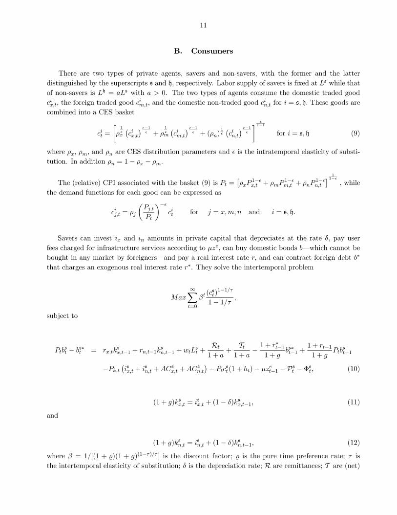
B. Consumers

There are two types of private agents, savers and non-savers, with the former and the latter

distinguished by the superscripts s and h respectively. Labor supply of savers is fixed at s while that

of non-savers is h = s with 0. The two types of agents consume the domestic traded good

, the foreign traded good , and the domestic non-traded good for = s h These goods are

combined into a CES basket

=

∙

1

¡¢ −1

+ 1

¡

¢ −1 + ()

1

¡¢ −1

¸ −1

for = s h (9)

where , , and are CES distribution parameters and is the intratemporal elasticity of substi-

tution. In addition = 1− − .

The (relative) CPI associated with the basket (9) is =£

1− +

1− +

1−

¤ 11−

while

the demand functions for each good can be expressed as

=

µ

¶− for = and = s h

Savers can invest and amounts in private capital that depreciates at the rate , pay user

fees charged for infrastructure services according to , can buy domestic bonds –which cannot be

bought in any market by foreigners–and pay a real interest rate and can contract foreign debt ∗

that charges an exogenous real interest rate ∗. They solve the intertemporal problem

∞X=0

(s)

1−1

1− 1

subject to

s − s∗ =

s−1 + −1

s−1 +

s +

R

1 + +

T1 +

− 1 + ∗−1

1 + s∗−1 +

1 + −1

1 +

s−1

−¡s + s +s +s

¢− s(1 + )− −1 − Ps −Φs (10)

(1 + )s = s + (1− )s−1 (11)

and

(1 + )s = s + (1− )s−1 (12)

where = 1[(1 + )(1 + )(1−) ] is the discount factor; is the pure time preference rate; isthe intertemporal elasticity of substitution; is the depreciation rate; R are remittances; T are (net)

12

transfers; denotes the consumption value added tax (VAT); and Φs are profits from domestic firms.

Remittances and transfers are proportional to the agent’s share in aggregate employment. Observe

that in the budget constraint (10), the trend growth rate appears in several places in (10)-(12),

reflecting the fact that some variables are dated at and others at -1 and that multiplies s and

s−1because domestic bonds are indexed to the price level.17 Also note that there are adjustment

costs incurred in changing the capital stock–s ≡ 2

³s

s−1− −

´2

s−1 for = and with

0–and portfolio adjustment costs associated with foreign liabilities–Ps ≡ 2(s∗ − s∗)2 where

∗ is the (initial) steady-state value of the private foreign liabilities.18

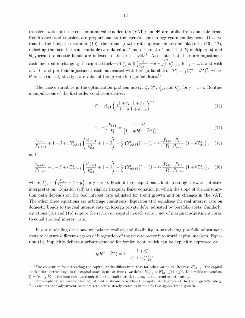
The choice variables in the optimization problem are s , s ,

s∗ ,

s, and s for = . Routine

manipulations of the first-order conditions deliver:

s = s+1

µ1 +

1 +

1 +

1 + +1

¶− (13)

(1 + )+1

=

1 + ∗£1− (s∗ − s∗)

¤ (14)

+1

+1

+ 1− + Υs+1

Ãs+1

s+ 1−

!−

2

¡Υs+1

¢2= (1 + )

+1

+1

¡1 + Υs

¢ (15)

and

+1

+1

+ 1− + Υs+1

Ãs+1

s+ 1−

!−

2

¡Υs+1

¢2= (1 + )

+1

+1

¡1 + Υs

¢ (16)

where Υs =³

ss−1− −

´for = Each of these equations admits a straightforward intuitive

interpretation. Equation (13) is a slightly irregular Euler equation in which the slope of the consump-

tion path depends on the real interest rate adjusted for trend growth and on changes in the VAT.

The other three equations are arbitrage conditions. Equation (14) equalizes the real interest rate on

domestic bonds to the real interest rate on foreign private debt, adjusted by portfolio costs. Similarly,

equations (15) and (16) require the return on capital in each sector, net of marginal adjustment costs,

to equal the real interest rate.

In our modelling decisions, we balance realism and flexibility in introducing portfolio adjustment

costs to capture different degrees of integration of the private sector into world capital markets. Equa-

tion (14) implicitly defines a private demand for foreign debt, which can be explicitly expressed as:

(s∗ − s∗) = 1− 1 + ∗(1 + )

+1

17The convention for detrending the capital stocks differs from that for other variables. Because s−1–the capital

stock before detrending–is the capital stock in use at time , we define s−1 ≡ s

−1(1 + ). Under this convention,

s = ( + )s in the long run–as required for the capital stock to grow at the trend growth rate .

18For simplicity, we assume that adjustment costs are zero when the capital stock grows at the trend growth rate .

This ensures that adjustment costs are zero across steady states as in models that ignore trend growth.

13

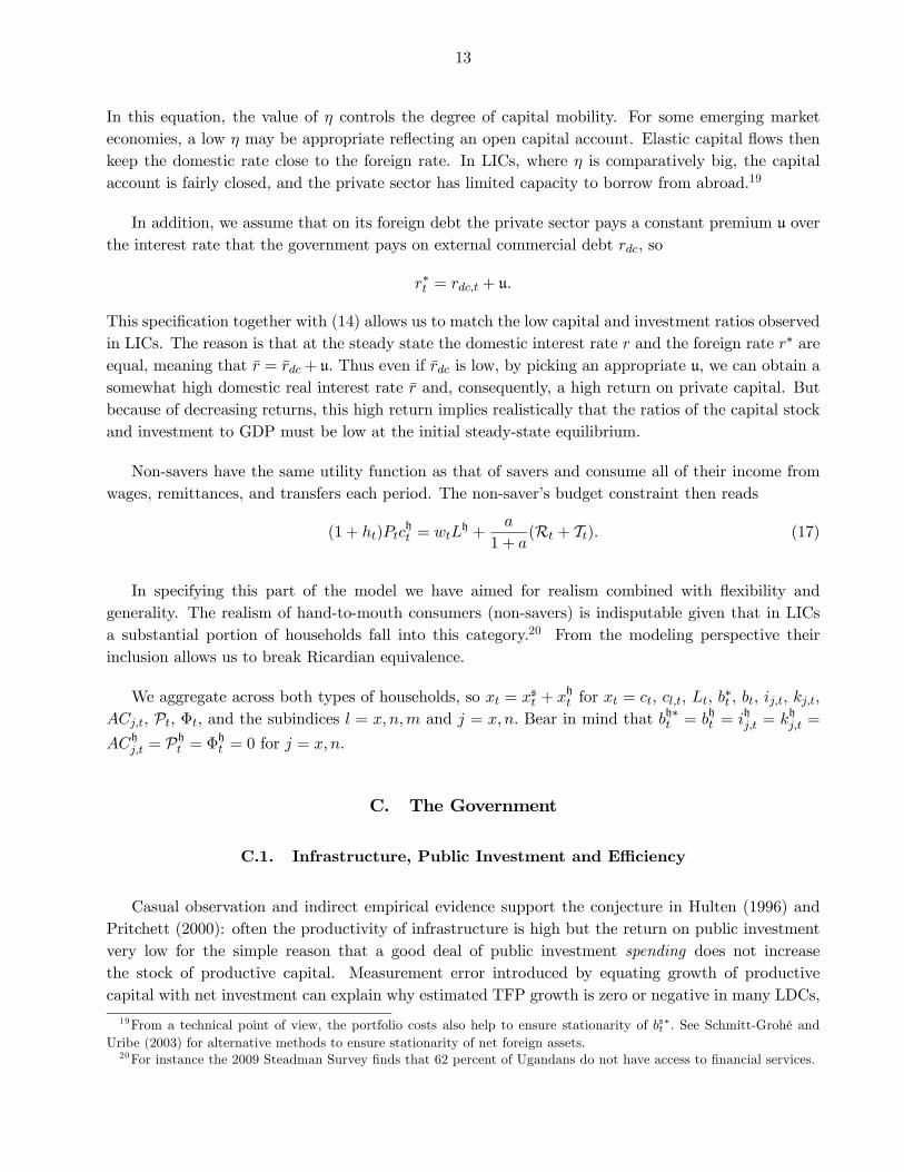
In this equation, the value of controls the degree of capital mobility. For some emerging market

economies, a low may be appropriate reflecting an open capital account. Elastic capital flows then

keep the domestic rate close to the foreign rate. In LICs, where is comparatively big, the capital

account is fairly closed, and the private sector has limited capacity to borrow from abroad.19

In addition, we assume that on its foreign debt the private sector pays a constant premium u over

the interest rate that the government pays on external commercial debt , so

∗ = + u

This specification together with (14) allows us to match the low capital and investment ratios observed

in LICs. The reason is that at the steady state the domestic interest rate and the foreign rate ∗ areequal, meaning that = + u Thus even if is low, by picking an appropriate u we can obtain a

somewhat high domestic real interest rate and, consequently, a high return on private capital. But

because of decreasing returns, this high return implies realistically that the ratios of the capital stock

and investment to GDP must be low at the initial steady-state equilibrium.

Non-savers have the same utility function as that of savers and consume all of their income from

wages, remittances, and transfers each period. The non-saver’s budget constraint then reads

(1 + )h =

h +

1 + (R + T). (17)

In specifying this part of the model we have aimed for realism combined with flexibility and

generality. The realism of hand-to-mouth consumers (non-savers) is indisputable given that in LICs

a substantial portion of households fall into this category.20 From the modeling perspective their

inclusion allows us to break Ricardian equivalence.

We aggregate across both types of households, so = s + h for =

∗

P Φ and the subindices = and = Bear in mind that h∗ =

h =

h =

h =

h = Ph = Φh = 0 for = .

C. The Government

C.1. Infrastructure, Public Investment and Efficiency

Casual observation and indirect empirical evidence support the conjecture in Hulten (1996) and

Pritchett (2000): often the productivity of infrastructure is high but the return on public investment

very low for the simple reason that a good deal of public investment spending does not increase

the stock of productive capital. Measurement error introduced by equating growth of productive

capital with net investment can explain why estimated TFP growth is zero or negative in many LDCs,

19From a technical point of view, the portfolio costs also help to ensure stationarity of s∗ See Schmitt-Grohé and

Uribe (2003) for alternative methods to ensure stationarity of net foreign assets.20For instance the 2009 Steadman Survey finds that 62 percent of Ugandans do not have access to financial services.

14

as suggested by Pritchett (2000); and why empirical studies generally find a much stronger positive

relationship between growth and physical indicators of infrastructure than between growth and capital

stock series calculated via the perpetual inventory method, as reviewed by Straub (2008).21

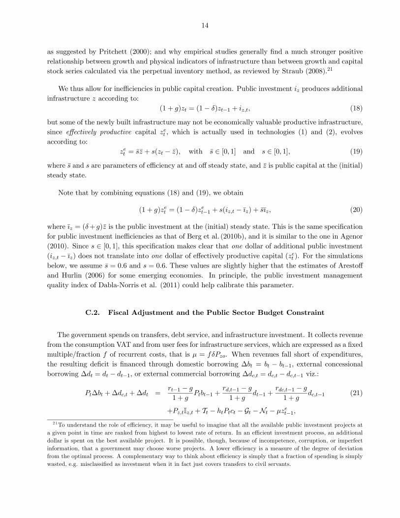
We thus allow for inefficiencies in public capital creation. Public investment produces additional

infrastructure according to:

(1 + ) = (1− )−1 + (18)

but some of the newly built infrastructure may not be economically valuable productive infrastructure,

since effectively productive capital which is actually used in technologies (1) and (2), evolves

according to:

= + ( − ) with ∈ [0 1] and ∈ [0 1] (19)

where and are parameters of efficiency at and off steady state, and is public capital at the (initial)

steady state.

Note that by combining equations (18) and (19), we obtain

(1 + ) = (1− )−1 + ( − ) + (20)

where = (+) is the public investment at the (initial) steady state This is the same specification

for public investment inefficiencies as that of Berg et al. (2010b), and it is similar to the one in Agenor

(2010). Since ∈ [0 1] this specification makes clear that one dollar of additional public investment( − ) does not translate into one dollar of effectively productive capital (

). For the simulations

below, we assume = 06 and = 06 These values are slightly higher that the estimates of Arestoff

and Hurlin (2006) for some emerging economies. In principle, the public investment management

quality index of Dabla-Norris et al. (2011) could help calibrate this parameter.

C.2. Fiscal Adjustment and the Public Sector Budget Constraint

The government spends on transfers, debt service, and infrastructure investment. It collects revenue

from the consumption VAT and from user fees for infrastructure services, which are expressed as a fixed

multiple/fraction of recurrent costs, that is = . When revenues fall short of expenditures,

the resulting deficit is financed through domestic borrowing ∆ = − −1 external concessional

borrowing ∆ = − −1 or external commercial borrowing ∆ = − −1 viz.:

∆ +∆ +∆ =−1 −

1 + −1 +

−1 −

1 + −1 +

−1 −

1 + −1 (21)

+I + T − − G −N − −1

21To understand the role of efficiency, it may be useful to imagine that all the available public investment projects at

a given point in time are ranked from highest to lowest rate of return. In an efficient investment process, an additional

dollar is spent on the best available project. It is possible, though, because of incompetence, corruption, or imperfect

information, that a government may choose worse projects. A lower efficiency is a measure of the degree of deviation

from the optimal process. A complementary way to think about efficiency is simply that a fraction of spending is simply

wasted, e.g. misclassified as investment when it in fact just covers transfers to civil servants.

15

where , , G, andN denote concessional debt, external commercial debt, grants, and natural resource

revenues (if any);22 and and are the real interest rates (in dollars) on concessional and commercial

loans. The interest rate on concessional loans is assumed to be constant = while the interest

rate on external commercial debt incorporates a risk premium that depends on the deviations of the

external public debt to GDP ratio³+

´from its (initial) steady-state value

³+

´. That is,

= +

+

− +

(22)

where is a risk-free world interest rate and = + is GDP. Van der Ploeg and Venables

(2011) provide positive estimates for . But note by setting 0 and = 0 our specification

embeds the case of an exogenous risk premium that does depend on public debt.

The term I in the budget constraint (21) corresponds to public investment outlays includingcosts overruns associated with absorptive capacity constraints. It is defined as

I = H( − ) +

Because skilled administrators are in scarce supply in LICs, ambitious public investment programs

are often plagued by poor planning, weak oversight, and myriad coordination problems, all of which

contribute to large cost overruns during the implementation phase.23 To capture this, we multiply

new investment ( − ) by H =³1 +

−1− −

´, where ≥ 0 determines the severity of the

the absorptive capacity–or “bottleneck”–constraint in the public sector. The constraint affects only

implementation costs for new projects: in a steady state,¡1 +

− −

¢= 1 as = ( + ).

Policy makers accept all concessional loans proffered by official creditors. The borrowing and

amortization schedule for these loans is fixed exogenously. Given the paths for public investment and

concessional borrowing, the fiscal gap before policy adjustment (Gap) can be defined as:

Gap =1 +

1 + −1−+

−1 −

1 + −1+

−1 −

1 + −1+I+T−−G−N−−1 (23)

That is, Gap corresponds to expenditures (including interest rate payments on debt) less revenues and

concessional borrowing, when transfers and taxes are kept at their initial levels Tand , respectively.Using this definition, we can rewrite the budget constraint (21), in any given year, as:

Gap = ∆ +∆ + ( − ) − (T − T) (24)

In the short/medium run, this gap Gap in (24) can be covered by domestic and/or external

commercial borrowing ∆ + ∆, tax adjustments ( − ) and/or transfers adjustments

−(T − T) For the sake of comparing different borrowing schemes, in the experiments below, we will22We model natural resources revenues as a net foreign transfer, following Dagher et al. (2012). As such the measure

of GDP used below corresponds to non-oil GDP. For a more comprehensive analysis of oil production, foreign investment,

and managing natural resources in LICs see Berg et al. (2012).23Development agencies report that cost overruns of 35% and more are common for new projects in Africa. The most

important factor by far is inadequate competitive bidding for tendered contracts. See Foster and Briceno-Garmendia

(2010).

16

focus on cases where part of this gap can be filled with either external commercial loans or domestic

loans, but not with both at the same time.

Debt sustainability requires, however, that the VAT and transfers eventually adjust to cover the

entire gap (i.e., ∆ + ∆ = 0). We let policy makers divide the burden of adjustment (net

windfall when Gap 0) between transfers cuts and tax increases. The adjustments, defined below

according to some reaction functions, have as part of their targets the following debt-stabilizing values

for transfers and the VAT

target = + (1− )

Gap

(25)

and

T target = T − Gap (26)

where is a policy parameter that splits the fiscal adjustment between taxes and transfers and therefore

satisfies 0 ≤ ≤ 1 For the extreme case of = 0 (respectively = 1) all the adjustment falls on taxes(respectively transfers).

Taxes and transfers are defined according to the following reaction functions:

= (27)

and

T =nT T

o (28)

where is a ceiling on taxes, T is a floor for transfers, and and T are determined by the fiscal

rules

= −1 + 1(target − −1) + 2

(−1 − target)

with 1 2 0 (29)

and

T = T−1 + 3(T target − T−1)− 4(−1 − target) with 3 4 0 (30)

with = + and = or depending on whether the rules respond to domestic debt or

commercial debt. The target for debt target is given exogenously. The ceiling on taxes and the

floor T on transfers can also have discrete jumps over time, as we show below.24 This allows us to

model staggered tax and transfers structures.

Given the targets, the reaction functions defined in (27)-(30) together with the budget constraint

(24) embody the core policy dilemma. Fiscal adjustment is painful, especially when administered sud-

denly in large doses. The government would prefer therefore to phase-in tax increases and expenditure

cuts slowly (1 0 and 3 0). Since fiscal adjustment is gradual, the debt instrument that varies

endogenously to satisfy the government budget constraint may rise above its target level in the time

it takes and T to reach target and T target . When this happens, the transition path includes a

phase in which T T target and/or target to generate the fiscal surpluses needed to pay down

the debt. In addition, and despite the fact that the rules respond to debt (i.e., 2 0 and 4 0), if

the government moves too slowly (i.e., 1 and 3 are too low), or if the bounds and T constrain

24For instance, to introduce discrete jumps in the cap on taxes we can respecify the rule as = , where = +∆

is the initial cap and ∆ is a discrete jump (shock) at time which can be temporary or permanent.

17

adjustment too much, interest payments will rise faster than revenue net of transfers, causing the debt

to grow explosively. Large debt-financed increases in public investment are undeniably risky–the

economy converges to a stationary equilibrium only if policy makers win the race against time.

D. Market-Clearing Conditions and External Debt Accumulation

Flexible wages and prices ensure that demand continuously equals supply in the labor market

+ = (31)

where the labor supply = s + h is fixed.

In the non-tradables market, after aggregating across types of consumers, we obtain

=

µ

¶− + ( + + +) + I (32)

The first term of the right-hand side of (32) is the demand for non-traded consumer goods, while the

second and third terms link public and private investment to orders for new capital goods.

Finally, aggregating across consumers and adding the public and private sector budget constraints

produce the accounting identity that growth in the country’s net foreign debt equals the difference

between national spending and national income:

− −1 + − −1 + ∗ − ∗−1 = −

1 + −1 +

−1 −

1 + −1 +

∗−1 −

1 + ∗−1 (33)

+P + I + ( + + +)

+ − − −R − G −N

Equation (33) includes extra terms that reflect the impact of trend growth on real interest costs and

the contributions of remittances, grants, and natural resource related foreign transfers to gross income.

The textbook identity emerges when = R = G = N = 0.

III. Calibration of the Model

Calibration of the model requires data on cost shares, elasticities of substitution, consumption

shares, depreciation rates, sector shares in GDP, tax rates, debt stocks, and the return on infrastructure

at the benchmark equilibrium. Once values are set for these parameters, all other variables that enter

the model can be tied down by budget constraints, the first-order conditions associated with the

solution to the private agents’ optimization problems, and various adding-up constraints.

The values in Table 1 are based on a mixture of data and guesstimates. We assume that =

= = = = = 1 and discuss below the rationale for the value assigned to each

parameter and the problems that arose in calibrating certain parts of the model:

18

• The distribution parameters ( ). In the base case, we pick and so that, the share

of non-tradables in GDP is about 50% and the share of imports in GDP is around 45%, which

correspond to average shares of non-tradables and imports for LICs during 1998-2008 using WEO

data. This gives us = 043 and = 037 Then is calculated as = 1− −

• Intertemporal elasticity of substitution (). According to Agenor and Montiel (1999), most

estimates of for LDCs lie between 010 and 050. The value in the base case, 034, equals the

average estimate for LICs in Ogaki et al. (1996).

• Elasticity of substitution in consumption (). We fix at 050 as estimates of compensated

elasticities of demand tend to be small at high levels of aggregation, especially when food claims

a large share of total consumption.25

• Capital’s share in value added ( ). Data on factor shares may be found in social accountingmatrices assembled by the Global Trade Analysis Project (GTAP) and the International Food

Policy Research Institute (IFPRI). The GTAP5 database for SSA suggests a capital share of

55 − 60% in the non-tradables sector and 35 − 40% in the tradables sector.26 The data in

Thurlow et al. (2004) and Perrault et al. (2010) suggest similar numbers.27 Accordingly, we set

= 055 and = 040.

• Learning externalities ( ). The base case does not incorporate learning externalities.In alternative runs that allow for learning effects, and are set to 008 so that the social

return to capital in the traded sector is about 30% higher than the private return.28

• Cost share of non-traded inputs in the production of capital goods ( ). Data on the ratio ofimported machinery and equipment to aggregate investment indicate that and are around

05 in SSA. One-half is also the guesstimate used by the IMF (2007a) in its analysis of scaling

up public investment in Nigeria.

• Elasticities of sectoral output with respect to the stock of infrastructure ( ). The ratio

is set independently. This ratio and other values assigned elsewhere in calibrating the model–

most notably, the return on infrastructure–pin down and .29 We assume = 1 in

all runs and obtain that = 017

• Depreciation rate (). There is little hard data on depreciation rates in LICs. Our choice of 5%is in line with estimates for developed countries.

25See Lluch et al. (1977, chapter 3), Deaton and Muellbauer (1980, p.71), Blundell (1988, p.35), and Blundell et al.

(1993, Table 3b).26The nontradables sector comprises trade and transport, private services, dwellings, and construction. The tradables

sector consists of agriculture and manufacturing.27The average factor shares cited here conceal tremendous variation. For example, the value added share of capital in

the services sector is 59% in Zambia but only 27% in Malawi. See Thurlow et al. (2004) and Thurlow et al. (2008).28The net social return to capital, evaluated at a steady state is ( + )(1 + ) − . To set so that the social

return is 30% above the private return, solve ( + )(1 + )− = (130) for .29 and are linked to other parameters and variables through = ( + )(+), where = +

is the gross return on infrastructure, is the share of sector j production in GDP, and is the ratio of infrastructure

investment to GDP.

19

Table 1

Base Case Calibration

Parameter Value Definition

0.43 Distribution parameter for non-traded goods

0.37 Distribution parameter for traded goods

0.34 Intertemporal elasticity of substitution

0.50 Intratemporal elasticity of substitution across goods

0.40 Capital’s share in value added in the traded sector

0.55 Capital’s share in value added in the non-traded sector

0.00 Capital learning externalities

0.00 Sectoral output learning externalities

0.50 Cost share of non-traded inputs in the production of capital

0.17 Elasticities of sectoral output with respect to infrastructure

0.05 Depreciation rate

6.41 Capital adjustment cost parameter

0.05 User fees parameter for infrastructure services

0.015 Trend growth rate

0.10 Initial real interest rate on domestic debt

∗ 0.10 Initial real interest rate on private external debt

0.04 Real risk-free foreign interest rate

0.00 Real interest rate on concessional loans

0.06 Initial real interest rate on public commercial loans

1.00 The portfolio adjustment costs parameter

0.00 Public debt risk premium parameter

u 0.04 Private debt risk premium

0.02 Public debt risk premium

0.25 Initial return on infrastructure

0.20 Initial public domestic debt to GDP ratio

0.50 Initial public concessional debt to GDP ratio

0.00 Initial public external commercial debt to GDP ratio

∗ 0.00 Initial private external debt to GDP ratio

G 0.05 Grants to GDP ratio

R 0.04 Remittances to GDP ratio

N 0.00 Natural Resource Revenues to GDP ratio

0.06 Initial ratio of infrastructure investment to GDP

0.60 Efficiency of public investment

0.00 Absorptive capacity parameter

0.15 Initial consumption VAT

T 11.93 Initial transfers to GDP ratio

0.00 Division of fiscal adjustment parameter

1 3 0.25 Fiscal reaction parameters (policy instrument terms)

2 4 0.02 Fiscal reaction parameters (debt terms)

1.50 Labor ratio of non-savers to savers

Note: See the calibration discussion in the main text.

20

• The capital adjustment costs parameter ( ). Evaluated at the initial equilibrium, this parameteris related to Ω, the elasticity of investment with respect to Tobin’s q, according to Ω = 1( +

).30 There are no reliable estimates of this elasticity for LICs. The assigned value, 2, is at the

high end of estimates for developed countries. This implies = 641 The results do not change

substantively when Ω equals 1 or 10.

• The user fees for infrastructure services (). The user fee for infrastructure services is a fixedmultiple/fraction of recurrent costs = . Fuel taxes, which are earmarked for road

maintenance and construction, electricity tariffs, and user charges for water and sanitation are

low but not trivial in LICs. According to Briceño-Garmendia et al. (2008), on average, user

fees recoup 50% of recurrent costs in SSA. Again, however, there is considerable variation–

Zambia’s average electricity tariff was three cents per kWH in 2008. We decided therefore to

let vary from 020 to unity, with = 050 in the base case. Since in the baseline calibration

=1

1− = 2 and = 005, then = 005.

• Trend growth rate (). The trend growth rate of 15% equals the 1990-2008 per capita growth

rate for SSA reported in African Development Indicators.

• The real interest rate on domestic bonds (), the real return on private capital, and the realinterest rate on external private debt ( ∗). Across steady states, the real interest rate on domesticdebt and the real return on private capital equal (1 + )(1 + ) − 1 where is the subjectivediscount rate. We choose jointly with and so that the domestic real interest rate is 10% at

the initial equilibrium. This is consistent with the data for SSA in Fedelino and Kudina (2003),

with the estimated return on private capital in Dalgaard and Hansen (2005), and with the

stylized fact that domestic debt in low- and middle-income countries is usually more expensive

than external commercial debt. There is tremendous variation in real interest rates across

countries and time periods, however. Note that at the steady state equation (14) implies that

the interest rate that the private sector pays on foreign debt must satisfy ∗ = So for the base

case we also have ∗ = 010

• The risk-free foreign real interest rate ( ). We fix at 4%, the approximate average of the

historical real returns on stocks and 3-10 year T bills in the United States.

• Real interest rates on concessional and non-concessional loans ( ). Ghana paid 87% on the$750 mn.Eurobond it floated in 2007. This is slightly above Gueye and Sy’s (2010) estimate of

the average interest rate SSA pays (855%) on debt raised in external capital markets, excluding

Seychelles and South Africa. The IMF-WB’s DSAs show an average interest rate of 23% on

concessional loans taken out by LICs in 2009-2010. Assuming 25% inflation in world prices of

traded goods, the corresponding (initial) real rates in dollars are about 6% for commercial debt

and 0% for concessional debt. The latter is assumed to be constant through the analysis.

30 In each sector , the first-order condition for investment reads [1 + (−1 − − )] = , where and

are the multipliers associated with the budget constraint and the law of motion for the capital stock. Since

is the

shadow price of capital measured in dollars,

is effectively Tobin’s , the ratio of the demand price to the supply

price of capital. Adopting this notation, we have that at a stationary equilibrium (+ )

= 1. Define Ω ≡ to be the

q-elasticity of investment spending. Then = 1( + )Ω.

21

• The portfolio adjustment costs parameter ( ) and the private and public debt risk premia pa-rameters (u ). The parameter controls the degree of openness of the capital account.

We set = 1 in the base case, to capture the fact that the private sector has limited access

to international capital markets. We assume that the public risk premium is constant–i.e.,

we set = 0 in equation (22)–and calibrate it as the difference between the interest rate on

public commercial debt and the risk-free foreign interest rate. So, at the initial steady state

equilibrium, = − = 002 The constant private risk premium is set as the difference

between the domestic interest rate and the interest rate on public commercial debt. Therefore

u = ∗ − = 004

• Return on infrastructure ().31 Estimates of the return on infrastructure are all over the map,

but the weight of the evidence in both micro and macro studies points to a high average return.

The median rate of return on World Bank projects circa 2001 was 20% in SSA and 15-29%

for various sub-categories of infrastructure investment. Foster and Briceño-Garmendia (2010)

estimate returns for electricity, water and sanitation, irrigation, and roads range from 17% to

24% Similarly, the macro-based estimates in Dalgaard and Hansen (2005) cluster between 15%

and 30% for a wide array of different estimators. Hulten et al. (2006), Escribano et al. (2008),

Calderón et al. (2009), and Calderón and Servén (2010) supply additional evidence of high re-

turns.32 All of this adds up to a presumption that high returns are the norm. We consider a

high-return scenario as the base case by setting = 025 at the initial steady state.33

• Domestic debt (). Different datasets give different numbers for the ratio of domestic debt toGDP in LICs. We settled on 20% by averaging the figures reported in IMF(2009a), Panizza

(2008), and Arnone and Presbitero (2010).

• Private foreign debt and public external debt ( ∗ ). We set concessional external debtequal to 50% of GDP at the initial equilibrium, given that the ratio of total public debt to GDP

and the share of concessional loans in total debt were about 70% and 69% respectively, for LICs

during 2007-2008.34 As little is known about the likely value of private foreign debt (or assets)

in LICs, we set ∗ = 0 for the base case. We also assume that initially the economy has no accessto external commercial loans implying that = 0

• Remittances, Grants, and Natural Resource Revenues (R, G N). For the base case, remit-

tances and grants are assumed to be 5% and 4% of GDP at their initial equilibrium, respectively.

These are in line with averages for LICs in the last decade. For the baseline calibration we assume

that the economy is not endowed with natural resources.

• Initial ratio of infrastructure investment to GDP ( ). We set the initial infrastructure invest-

ment to be equal to 6% of GDP This initial figure includes the net investment associated with

31The production function parameters and that govern are deduced from the calibration of , given the

rest of the calibration.32Some growth regressions suggest low or insignificant returns, but these are dominated by studies that use cumulative

public investment instead of physical indicators to measure the stock of instructure.33Thirty percent may raise some eyebrows, but it is not as big as some of the numbers thrown around in the literature

and in policy work. See for instance the scaling-up exercise in Box 4.1 in Barkbu et al. (2008) and Gupta, Powell, and

Yang (2006).34See IMF (2009a) and IMF staff calculations.

22

trend growth and the outlays on operations and maintenance (O+M)–which average about

34% of GDP for LICs in SSA.35 This figure is close to the average for LICs in SSA, which in

2008 corresponded to 609%, as suggested by Briceño-Garmendia et al. (2008).

• Efficiency of public investment ( ) and the absorptive capacity parameter ().36 The base

case assumes that investment is somewhat efficient ( = 060 and = 060) and that scaling

up does not strain absorptive capacity ( = 0 and = ). Motivated by the findings in Hulten

(1996), Pritchett (2000), and Foster and Briceño-Garmendia (2010), we also investigate scenarios

in which the scaling up is associated with extreme inefficiency ( = 02) and a tight absorptive

capacity constraint ( = 5).37

• Consumption VAT (). The consumption VAT in the model proxies for the average indirect

tax rate. Our rate of 15% at the initial steady state.38 This is comparable to the average

VAT of LICs, which using 2005-06 data by the International Bureau of Fiscal Documentation is

estimated to be close to 158%

• Net Transfers (T). At the initial steady state, transfers ensure that the budget constraint ofthe government holds. Given the other parameters we obtain T = 1193 percent of GDP. Giventhe definition of the other fiscal variables, this concept of transfers includes other taxes different

from VAT as well as non-capital expenditures such as public wages.

• Division of fiscal adjustment between expenditure cuts and tax increases (). Across steadystates, we assume that only taxes share the burden of fiscal adjustment ( = 0).

• Policy reaction parameters (1 2 3 4). There are no estimates of these parameters for LICs.

For the scenarios that allow commercial debt accumulation or domestic debt accumulation we

set 1 = 3 = 025 and 2 = 4 = 002 We also study the implications of lowering 1.

• Ratio of labor supply of non-savers to labor supply of savers (). We set = 15 so 60% percent

of the consumers are non-savers. This is broadly in line with survey findings in LICs.

35But true O+M costs are probably higher, as argued by Briceño-Garmendia et al. (2008). Because of underspending

on O+M, 30% of Africa’s infrastructure assets are in need of rehabilitation.36Appendix A describes how calibration of and interact with that of and the production function parameters

and . The bottom line is that the operator needs to be thoughtful when calibrating efficiency, particularly in

considering what it might imply for the marginal product of effective capital. A change in the calibration of the efficiency

has two different interpretations: (i) as a level change that applies to the past and the future, as when comparing

two countries at a point in time. In this case, should in principle change as well, but a change in is unnecessary,

because any effect of changing is undone by the change in and required to preserve the value of ; or (ii) as a

change that applies to future investment but not the past, as for example because of an improvement in public financial

management. It is up to the operator to decide which applies and whether other adjustments to the calibration are

necessary in light of that interpretation.37Pritchett’s estimates of range from 008 to 049 for SSA and from 009 to 054 for South Asia. In Africa, large

cost overruns stemming from planning/coordination/management problems and low capital budget execution ratios

(average = 66%) suggest that absorptive capacity may be a binding constraint in many countries. See Foster and

Briceño-Garmendia (2010).38For 2003-2006, consumption, indirect taxes, and trade taxes averaged 81%, 9.6%, and 4.6% of GDP, respectively. If

duties on consumer imports accounted for half of trade taxes, then the average consumption tax was 14.7%. (Data from

IMF, 2007b). Ideally this rate will also reflect VAT productivity adjustments.

23

The public investment scaling-up scenario we study is exogenous and front loaded. Concessional

borrowing and an increase in grants, which are also exogenous, help finance this scaling up.

The time lines for the infrastructure investment surge (valued at the initial price level = 2),

concessional borrowing, and the increase in grants, as percentage of initial GDP ( = 100), are shown

in Table 2. The time lines are hump-shaped. In year 1 public investment is at 6% of GDP and there is

no increase. Then the scaling up of this investment jumps to 5% of initial GDP in year 2, rises to 7%

in years 3 and 4, and tapers off gradually to its permanent level of 3% of initial GDP. Net concessional

loans, on the other hand, increase by 4% of GDP in year 2, go slightly up to 5% of initial GDP in year

3 and then decline gradually until year 9.39 From year 10 to year 28, the country repays these loans

(−101% of initial GDP). The increase in grants G corresponds to 04% of initial GDP from year 2 to

year 9, and declines to 02% before dying off by year 32. Concessional borrowing and the increase in

grants will only cover about 50% of the investment surge during the first 8 years of the scaling up. The

rest will require some fiscal adjustment and, potentially, other sources of financing such as external

commercial or domestic borrowing.

Table 2

Public Investment Scaling Up, Concessional Borrowing, and Grants

1 2 3 4 5 6 7 8 9 10 29 32

(−)

00 50 70 70 66 58 50 44 40 30 30 30

00 40 50 40 30 20 10 08 05 -101 00 00

G−G

00 04 04 04 04 04 04 04 04 02 02 00

Note: figures are in percent of initial GDP (= 100).

IV. The Long-Run Outcome

In this section, we use a mix of analytical and numerical methods to demonstrate that in the long

run (i) infrastructure and private capital are strong complements and (ii) increases in infrastructure

investment can be self-financing, depending on structural conditions of the economy.

39The repayment period is leisurely stretched out over 27 years, after 8 years of grace period. These correspond roughly

to the average maturity and grace-period years for new concessional loans to LICs in 2009-2010, based on available IMF-

WB’s DSAs. We assume that the country contracts a concessional loan of 2025% of initial GDP in year 2, with the

previously described disbursements. Then we apply an equal principal payment formula, together with these grace and

maturity periods and an interest rate of 0%, to obtain the repayment profile. The grant element of this loan is about

62%.

24

Z

O

K

K

C'

C

C'(z1)

C(z0)

FB'(T1)

FB(T0) T1>T0iz

zc

k

iz,1

iz,0

k0

k1

c1 c0 z1zo

Figure 1: The Long-run Outcome in the Simplified Model.

A. Insights From a Simplified Model

Although the model of Section II has many moving parts, it is not a black box. To highlight

the key interactions that drive the long-run (steady-state) outcome, consider a stripped-down model

that ignores trend growth, non-traded goods, foreign traded goods, private capital flows, remittances,

grants, natural resource revenues, public sector debt and efficiency and absorptive capacity issues (so

= = 1 and = 0). For notational simplicity we ignore the upper bars on the variables, which

we used before to denote steady-state values. With these elements gone, the steady-state equilibrium

simplifies to

= +1− (34)

+ = +−11− (35)

= (36)

+ = + T (37)

and

= − ( + ); (38)

five equations that can be solved for , , , and either T or as a function of . Equation (34) is theproduction function and equations (35)-(38) are the steady-state versions of equations (8), (18),(21),

and (33) in Section II.

25

Figure 1 depicts the steady-state equilibrium when transfer payments adjust to satisfy the govern-

ment budget constraint, but similar results obtain if all the fiscal adjustment falls on taxes. The ray

OZ in the first quadrant relates to . For the results that follow, it is important to note the obvious:

the slope of OZ is quite flat because comparatively small increases in map into very large increases

in over the long run ( = ).

Proceeding south, the KK schedule in the fourth quadrant shows how the equilibrium private

capital stock depends on the stock of infrastructure. From (35),

=

µ

¶µ

1− −

¶ 0 (39)

Substitute = +

and = =

+into (39), where = − is the net return to infrastructure

and =is the marginal product of infrastructure. After canceling terms, we have

¯

=

µ+

+

¶µ

1− −

¶ (40)

Since we have assumed a Cobb-Douglas technology, growth in the stock of infrastructure stimulates

private investment by increasing the marginal product of capital. Equation (40) tells us, in addition,

that the long-run crowding-in effect may be quantitatively large. The ratio of the gross return on

infrastructure to the gross return on private capital, ++

, multiplies a term that lies somewhere

between 049 and 183, if ∈ [033 055] and ∈ [0 015]. Thus, if empirical estimates are right andthe mean return on infrastructure is much higher than the mean return on private capital, then the

long-run crowding-in coefficient can approach or exceed two. Suppose, for example, that = 010,

= 025, = 005, and = 040 as there is only one domestic traded good. The crowding-in coefficientthen ranges from about 133 to 178 when ∈ [0 015]. Productive infrastructure and private capital

are very strong complements in the long run. This, however, depends on structural conditions of the

economy. As we will see below, public investment inefficiencies and absorptive capacity constraints,

among others, can lower the crowding in.

The schedules in the second and third quadrants connect the increases in the stocks of infrastructure

and private capital to consumption, tax revenue, and the change in transfers needed to balance the

fiscal budget. CC relates to for given , while FB depicts the locus in the - plane for which

revenue equals government expenditure. The slope of CC equals ( + )(1 + ) − , the net social

marginal product of capital. The FB schedule

| =− T1−

has a horizontal intercept at = Tand a positive slope that rises from at = 0 to infinity at = .

When increases, the CC schedule shifts horizontally to the left by (1 − ). Crowding-in of

private capital increases consumption another [( + )(1 + ) − ](1 − ). Expressed relative to

the policy instrument , the combined effect is

=

∙µ +

+

¶+

1− − +

¸

26

Comparing the increase in consumption taxes and user fees (+ = + ) to the increase

in investment determines whether the FB schedule shifts left or right. In Figure 1 the revenue gain

pays for the increase in investment and leaves something left over to finance higher transfer payments.

This case occurs when

(1 + −

)(1− − )

³1−

+

´ − (41)

The crucial implication of (41) is that does not have to be unusually high for the increase in

infrastructure investment to be self-financing. Consider the base case values of Table 1 but bear

in mind that in this simplified model = 040 (since there is only one domestic traded good) and

= 0025 (since = and = 050) In this case, the borderline value of is a modest 10%. Even

with = 0, however, (41) holds for 215%. This is high but well within the range of empirical

estimates. Moreover, note that this borderline value decreases with the externalities .

B. Numerical Solutions

Table 3 summarizes the long-run effects of a permanent increase in public investment equal to

3% of initial GDP using the full model. Consider first the base case. Transfers are kept constant,

by assumption, while taxes require a small adjustment from 15% to 163%. As predicted by the

simplified model, the crowding-in coefficient, calculated as ∆∆

exceeds unity. Consequently there

are some gains in the economy. Real output, real wages, and private capital increase by more than

13% while consumption rises by 93%. Sectoral outputs also move up, and there is a permanent real

depreciation of 19%. Our base case calibration then delivers a positive scenario, to some extent. But

even with a rate of return on public capital of 25% the public investment does not pay for itself. The

average tax rate is quite low, and most of the benefits accrue to the private sector are not sufficient

to cover the recurrent costs.

The long-run impact of the public investment scaling up depends on the structural conditions of

the economy. To see this, consider scenario 1 of Table 3. This scenario is very optimistic. The return

on capital is 35% user fees recoup all recurrent costs–i.e., = 1 implying that = = 01–the

public investment surge is fully efficient = 1, and there are some positive externalities = 008,

which imply a social return to capital in the traded sector that is 30% higher than the private return.

With these conditions, the scaling up turns out to be more than self-financing and produces striking

benefits in the real economy. Taxes decline to 123% in the long run, while real GDP, wages, and

private capital expand by about 33 − 35%, as the crowding-in coefficient is above 2 Furthermore,consumption jumps by 293%.

We issue two caveats.

First, it is also possible to recreate very troublesome scenarios under weak structural conditions

that may characterize some LICs. Scenario 2 in Table 3 is an example. This scenario features a low

return on public capital = 010, a deficient collection rate of user fees of 20% of recurrent costs–

i.e., = 02 implying that = = 002–and an insignificant efficiency of additional public

27

investment = 02. As a result, taxes have to adjust permanently to 187% and consumption falls by

12%.40 In addition, real GDP and private capital have disappointing increases of about 25% despite

the large increase in public investment. All of this is consistent with a crowding-in coefficient that is

below 1.

Table 3

Long-run Effects of Scaling Up Public Investment by 3 Percent of Initial GDP

Base Case Scenario 1 Scenario 2

= 025 = 006 = 035 = 01 = 010 = 002

= 060 and = 0 = 1 and = 008 = 02 and = 0

Taxes 16.29 12.26 18.73

CIC ∆(+)∆

1.51 2.31 0.85

Public Effective Capital 50.00 83.33 16.67

Private Capital + 13.23 33.70 2.49

Real GDP 13.45 34.31 2.48

Real Wages 13.53 34.66 2.44

Consumption 9.29 29.30 -1.24

Traded Output 13.83 35.99 2.21

Non-Traded Output 13.04 32.57 2.75

Real Exchange Rate -1.90 -3.90 -0.36

Note: The effects are measured as the percentage change between the steady states, except

for taxes and the crowding-in coefficient (CIC). Fiscal adjustment is assumed to fall exclusively

on taxes, so transfers are kept constant.

The second caveat pertains to difficulties that may arise on the transition path. As we will show

in the next section, even when the long run looks good, medium-run tax increases appear to be

unavoidable. Non-concessional borrowing can smooth away difficult fiscal adjustments that threaten

to undermine support for the investment program. But if the capacity for fiscal adjustment is too

limited and the government borrows too much in the short/medium run, there is a risk that future

revenue gains will not arrive fast enough to prevent explosive growth of the debt. Therefore, the

viability of the borrowing-for-development strategy depends not only on the structural conditions of

the economy and the long-run outcome, but also on whether policy makers can solve the problem of

how to get from here to there.

40Note that the adjustment in taxes would be smaller if government transfers were cut. But this is not an easy task

when public sector employees are pressing for wage increases that match the increase in the private sector wages.

28

V. The Medium-Term Fiscal and Macroeconomic Adjustments

Under Different Financing Schemes

A. Unconstrained Tax Adjustment

There are a variety of ways to finance a large increase in public investment. We start by analyzing

the case in which, given the public investment surge and the path for concessional borrowing and

grants, taxes and/or transfers adjust continuously and freely to satisfy the budget constraint of the

government. This provides the counterfactual for the analysis of riskier schemes that supplement

concessional borrowing with domestic or external commercial loans.

For now, we assume the government is unable or unwilling to take out non-concessional debt.

Commercial and domestic debt thus stay at their initial steady-state levels; so = = and

= = . Taxes and transfers adjust continuously and without bounds. To capture this we set

→∞ T →∞, 1 = 3 = 1 and 2 = 4 = 0 in equations (27)-(30) and combine them with (25)

and (26) to obtain

= target and T = T target

To fix ideas and simplify the analysis, in the experiments below we assume the burden of fiscal

adjustment falls exclusively on taxes. In other words, we set = 0 This implies that transfers are

kept constant at their initial level T = T target = T, while taxes follow the path = target which,

given 1 = 1 and 2 = 0 ensures that taxes always adjust to satisfy the government budget constraint.

A.1. The Base Case

The medium-run dynamics presented in Figure 2 are discouraging.41 Since cumulative borrowing

and grants in years 2-9 equals about 50% of cumulative net investment, the fiscal adjustment has to be

demanding. The VAT rises to 189% at = 5 and to 188% at = 10. The former increase is associated

with the demands from the scaling up, while the latter is related to the needs for concessional debt

repayment. Although conditions improve slightly thereafter, by year 20, the VAT still remains above

18%.

The government’s protracted fiscal problems in the first years also stem from disappointing effects

on private consumption and investment. Unfortunately, this disappointment is a robust feature of the

transition path. Because savers cannot smooth consumption by borrowing from abroad (imperfect

capital mobility) and non-savers live hand to mouth, the sharp increase in taxes translates into a

reduction in consumption. The positive impact of increases in the stock of infrastructure on future

productivity could spur, in theory, an immediate increase in private investment. But this is not

41The numerical simulations are free of approximation error. In all scenarios, the simulations track the global nonlinear

saddle path. The solutions were generated by set of programs written in Matlab 7.7.0.471 (R2008b) and Dynare 4.1.1.

See http://www.cepremap.cnrs.fr/dynare.

29

5 10 15 20 25 30

-10

0

10

Scaling Up (% of GDP)

Public Investment

Loans and Grants

5 10 15 20 25 30-5

0

5

10Relative Price of NT Goods

5 10 15 20 25 30

16

18

20Taxes (%)

5 10 15 20 25 30-1

0

1Transfers Change (% of GDP)

5 10 15 20 25 3010

11

12Interest Rate (%)

5 10 15 20 25 30-2

0

2

4

6

8Private Investment

5 10 15 20 25 30-10

0

10External Private Debt (% of GDP)

5 10 15 20 25 30-2

0

2

4

6Consumption

5 10 15 20 25 30

0

5

10Wages

5 10 15 20 25 300

20

40

Public Effective Capital

5 10 15 20 25 30

0

2

4

6Private Capital

5 10 15 20 25 301

2

3

4Real GDP Growth (%)

5 10 15 20 25 30-5

0

5

10Sectoral Output

Traded

Non-Traded

5 10 15 20 25 30

0

5

10Deficits (% of GDP)

Fiscal

Current Account

5 10 15 20 25 3040

50

60

70Concessional Debt (% of GDP)

5 10 15 20 25 3050

60

70

80

90Total Public Debt (% of GDP)

Figure 2: Base Case: Unconstrained Tax Adjustment. The transition path in the base case

when the government takes out only concessional loans and the tax adjustment is unconstrained.

Variables are expressed as percentage deviations from the initial steady state, unless otherwise noted.

30

possible. In our base case, the increase in the real interest rate–a by-product of the significant VAT

adjustment–is enough to force savers to cut investment in the short run.42 In summary, private

consumption and investment contract relative to their initial steady state in the short run: by the

year 2 consumption and investment decrease by about 1% and then stay depressed for another couple

of years before they start rising slowly.

Due to the period of stagnant investment, growth of the private capital stock and real income lag far

behind growth in the stock of infrastructure. At the typical 20-year horizon of the Excel-based DSAs

and relative to the steady state, public capital has increased almost 45% which corresponds to the 90%

of the 50% increase across steady states; but private capital is only about 33% higher (vs. almost 13%

higher across steady states).43 Growth (in per capita terms) increases above 2% in the first decade, but

by year 20 is close to 18% which is only 03 percentage points higher than the exogenously assumed

long-run growth rate of 15% Because income and the tax base grow slowly during the borrowing

phase, the government is ill-prepared for the subsequent repayment phase. The revenue demands of

debt service keep the VAT above 18%, which, in turn, slows the pace of capital accumulation and

perpetuates the fiscal bind. Eventually policy makers are rewarded for their perseverance with a tiny

revenue windfall and a moderate increase in the private capital stock, but this occurs in a distant

future.

As expected, total public debt follows the sustainable path of concessional debt. Public debt peaks

at year 8 reaching 84% of GDP and then declines as the country repays the concessional loans and GDP

increases. Because, by construction, taxes always adjust to satisfy the government budget constraint,

unstable dynamics for debt are ruled out from the analysis. Therefore the key question from the fiscal

perspective is whether the tax adjustment is feasible in practice. For the base case, an increase from

15% to 189% of the VAT in four years seems implausible.

A.2. More Optimistic and Troublesome Scenarios

We study now the dynamic implications of changing some of the structural conditions of the

economy. We consider conditions that represent optimistic and troublesome scenarios.

Panel A of Figure 3 shows the paths of the tax rate, consumption, and private investment of an

optimistic scenario. The initial return on infrastructure is 35%, user fees pay for all recurrent costs

= 1 ( = 01), and the public investment surge is fully efficient = 1. The paths of this scenario are

notably better than those from the base case, especially in the medium term. The peak of the VAT,

which occurs in the short run, is still high and close to 18%. But the medium-term tax is much more

42To see why the interest rate rises when taxes go up significantly, recall the Euler equation for savers consumption,

which can be written as:

=1 +

1 + +1

1 +

s+1

s

1

− 1

43 It is common practice to discount econometric estimates of the q-elasticity of investment and assign Ω a value of

5-10 to speed up adjustment of the capital stock. That does not work in our case. When Ω = 10, the increases in private

capital and real GDP are still small.

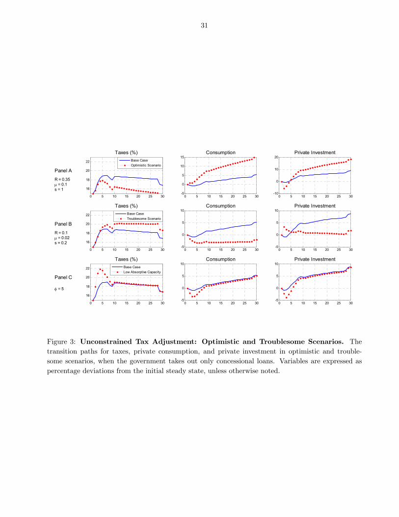
31

0 5 10 15 20 25 30

16

18

20

22

Taxes (%)

Panel A

R = 0.35 = 0.1s = 1

Base Case

Optimistic Scenario

0 5 10 15 20 25 30-5

0

5

10

15Consumption

0 5 10 15 20 25 30-10

0

10

20Private Investment

0 5 10 15 20 25 30

16

18

20

22

Taxes (%)

Panel B

R = 0.1 = 0.02s = 0.2

Base Case

Troublesome Scenario

0 5 10 15 20 25 30-5

0

5

10Consumption

0 5 10 15 20 25 30-5

0

5

10Private Investment

0 5 10 15 20 25 30

16

18

20

22

Taxes (%)

Panel C

= 5

Base Case

Low Absorptive Capacity

0 5 10 15 20 25 30-5

0

5

10Consumption

0 5 10 15 20 25 30-5

0

5

10Private Investment

Figure 3: Unconstrained Tax Adjustment: Optimistic and Troublesome Scenarios. The

transition paths for taxes, private consumption, and private investment in optimistic and trouble-

some scenarios, when the government takes out only concessional loans. Variables are expressed as

percentage deviations from the initial steady state, unless otherwise noted.

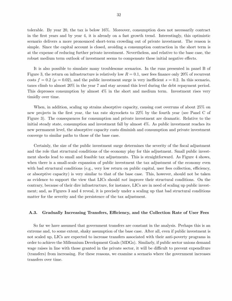
32

tolerable. By year 20, the tax is below 16%. Moreover, consumption does not necessarily contract

in the first years and by year 4, it is already on a fast growth trend. Interestingly, this optimistic

scenario delivers a more pronounced short-term crowding out of private investment. The reason is

simple. Since the capital account is closed, avoiding a consumption contraction in the short term is

at the expense of reducing further private investment. Nevertheless, and relative to the base case, the

robust medium term outlook of investment seems to compensate these initial negative effects.

It is also possible to simulate many troublesome scenarios. In the runs presented in panel B of

Figure 3, the return on infrastructure is relatively low = 01, user fees finance only 20% of recurrent

costs = 02 ( = 002), and the public investment surge is very inefficient = 02. In this scenario,

taxes climb to almost 20% in the year 7 and stay around this level during the debt repayment period.

This depresses consumption by almost 4% in the short and medium term. Investment rises very

timidly over time.

When, in addition, scaling up strains absorptive capacity, causing cost overruns of about 25% on

new projects in the first year, the tax rate skyrockets to 22% by the fourth year (see Panel C of

Figure 3). The consequences for consumption and private investment are dramatic. Relative to the

initial steady state, consumption and investment fall by almost 4%. As public investment reaches its

new permanent level, the absorptive capacity costs diminish and consumption and private investment

converge to similar paths to those of the base case.

Certainly, the size of the public investment surge determines the severity of the fiscal adjustment

and the role that structural conditions of the economy play for this adjustment. Small public invest-

ment shocks lead to small and feasible tax adjustments. This is straightforward. As Figure 4 shows,

when there is a small-scale expansion of public investment the tax adjustment of the economy even

with bad structural conditions (e.g., very low return on public capital, user fees collection, efficiency,

or absorptive capacity) is very similar to that of the base case. This, however, should not be taken

as evidence to support the view that LICs should not improve their structural conditions. On the

contrary, because of their dire infrastructure, for instance, LICs are in need of scaling up public invest-

ment; and, as Figures 3 and 4 reveal, it is precisely under a scaling up that bad structural conditions

matter for the severity and the persistence of the tax adjustment.

A.3. Gradually Increasing Transfers, Efficiency, and the Collection Rate of User Fees

So far we have assumed that government transfers are constant in the analysis. Perhaps this is an

extreme and, to some extent, shaky assumption of the base case. After all, even if public investment is

not scaled up, LICs are expected to increase transfers associated with their anti-poverty programs in

order to achieve the Millennium Development Goals (MDGs). Similarly, if public sector unions demand

wage raises in line with those granted in the private sector, it will be difficult to prevent expenditure

(transfers) from increasing. For these reasons, we examine a scenario where the government increases

transfers over time.

33

0 5 10 15 20 25 30

16

18

20Taxes (%) - Scaling Up

Panel ABase Case R vs R=0.10

Base Case Parameter Values Alternative Values

0 5 10 15 20 25 30

16

18

20Taxes (%) - No Scaling Up

0 5 10 15 20 25 30

16

18

20Taxes (%) - Scaling Up

Panel BBase Case vs

=0.020 5 10 15 20 25 30

16

18

20Taxes (%) - No Scaling Up

0 5 10 15 20 25 30

16

18

20Taxes (%) - Scaling Up

Panel CBase Case svss=0.2

0 5 10 15 20 25 30

16

18

20Taxes (%) - No Scaling Up

0 5 10 15 20 25 30

16

18

20

22

Taxes (%) - Scaling Up

Panel DBase Case vs

=5

0 5 10 15 20 25 30

16

18

20

22

Taxes (%) - No Scaling Up

Figure 4: Unconstrained Tax Adjustment: The Size of the Scaling Up. Comparison of the tax

adjustment with and without a scaling up of public investment, under different structural conditions.

The increase of public investment in the no scaling up scenario corresponds to 5% of the increase in

the scaling up scenario.

34

0 5 10 15 20 25 3015

16

17

18

19

20Taxes (%)

Panel A

IncreasingTransfers

Base Case Increasing Transfers and =0.5 and s =0.6

0 5 10 15 20 25 30

0

0.5

1

1.5Transfers Change (% of GDP)

0 5 10 15 20 25 30

0

2

4

6

8

10Consumption

0 5 10 15 20 25 3015

16

17

18

19

20Taxes (%)

Panel B

IncreasingTransfersWhen and sIncrease as Well

Base Case Increasing Transfers, , and s Over Time

0 5 10 15 20 25 30

0

0.5

1

1.5Transfers Change (% of GDP)

0 5 10 15 20 25 30

0

2

4

6

8

10Consumption

Figure 5: Unconstrained Tax Adjustment: Increasing Transfers. Comparison of the tax and

private consumption adjustments in the base case and in the case when government transfers, the

efficiency of public investment and user fees collection increase over time. Variables are expressed as

percentage deviations from the initial steady state, unless otherwise noted.

Our framework is flexible enough to incorporate different rules for transfers.44 For expositional

reasons, here we assume that transfers are raised as a fixed proportion m of increases in real GDP as

described by

T = T +mT( − )

where = + is real GDP at period . To fix ideas, assume m = 1.

When transfers increase over time, the damage report for the fiscal adjustment is grim, while the

consumption benefits are nil. As shown in panel A of Figure 5, taxes not only soar and reach a peak of

197% at = 7, but also stay above 19% over most of the debt repayment period. Of course transfers

grow, and by year 20 their increase is above 06% of GDP. However, their effect on consumption is fully

44When 0 the fiscal adjustment falls on both taxes and transfers. In this case the model can still allow for

scenarios with downwardly inflexible expenditure. For instance, transfers can be kept constant until growth generates a

fiscal windfall according to T = T target T where T target

is defined (26); or the government can be assumed to

be unable to cut other expenditures to offset increases in public sector wages, implying that transfers evolve as

T =

T target T + 005

( −)

where the initial public wage bill is 5% of GDP and raises of this bill are as large as raises in private sector wages.

35

offset by the more demanding tax adjustment. As a result, the path for consumption when transfers

increase is practically the same as that when transfers are kept constant.

Does this mean that, in the context of public investment scaling ups, LICs cannot raise transfers

without both suffering drastic tax adjustments and producing consumption benefits? The answer

may lie, once more, on the key role that structural conditions, such as efficiency of public investment

and the ability to collect user fees, play in the analysis. Unfortunately, there is evidence that these

structural conditions are weak in LICs. The public investment management quality index of Dabla-

Norris et al. (2011) suggests that there is a considerable variation across LICs. But their efficiency is

in general lower than that of emerging and advanced economies.45 On the other hand, average user

fees equal or slightly exceed average costs for operation and maintenances of physical infrastructure

in SSA. But because of low collection rates, revenues cover only half of recurrent costs, as discussed

by Briceño-Garmendia et al. (2008) and Eberhard et al. (2008).

Improving the efficiency of public investment and the collection rate of infrastructure user fees may

allow LICs to increase transfers, while easing fiscal adjustment. Raising both structural conditions to

100% would capture more revenue not only from the expansion of infrastructure services, but also from

services supplied by the existing network. Of course the prevalence of low efficiency and collection

rates suggest that the problem is not easy to solve. But the transition from partial to full efficiency and

collection does not have to occur overnight to greatly reduce the demands made on taxes. As shown in

panel B of Figure 5, even when it takes a decade to complete the task, by year 20 the VAT is reduced

to 162%, whereas the increase in transfers is about 125% of GDP. As more infrastructure-related

fiscal revenue is available, then the government can support a bigger increase in transfers than that of

an economy where efficiency and the collection rate do not improve. More importantly with less tax

adjustment and much higher transfers, consumption is boosted over the medium term.

Undoubtedly some governments will succeed in raising efficiency and the collection rate in upcoming

decades, but this poses new questions.

First, even when efficiency improves, it is not clear whether the collection rate would be expected

to rise or fall over time. The complicating factor is that scaling up public investment adds to the

collection task by increasing the share of the population with access to infrastructure services. If

collection capacity does not increase as fast as the supply of services, which is proportional to the

stock of effective infrastructure, the collection rate might fall.

Second, if steady, systematic increases in efficiency and the collection rate are sure to happen in

some country, then, given the magnitude of infrastructure deficits in LICs, policy makers should aim

to scale up investment even more. A country that can achieve the paths shown in panel B of Figure

5 might choose not settle for an increase in public investment of 3% of initial GDP in the medium

to long run; it could try to scale up much more. But this brings us back to the main scenario where

the challenge is to ascertain how the scope for scaling up depends on feasible fiscal adjustments in the

VAT.

45 In fact, public management capacity constraints in themselves may call for further investments in capacity, i.e. “to

invest in investing” in the words of Collier (2007).

36

B. Constrained Tax Adjustment Combined with External Commercial

Borrowing

The analysis of the previous section suggests that the transition can be challenging even when the

investment is self-financing in the long run. The most obvious remedy, investigated next, is to borrow

against future revenue gains in the external debt market with view to smoothing the path of fiscal

adjustment.

Increasingly LICs have access to external debt markets. In recent years, Uganda, Tanzania, Senegal,

Ghana, Angola, Congo DRC, Mali, Mauritania, and Rwanda have all entered into non-concessional

loan agreements or issued sovereign bonds in international capital markets. Recognizing that the

trend is likely to continue, the World Bank and the IMF have adopted a more flexible approach to

non-concessional borrowing. The World Bank has introduced the IDA Non-concessional Borrowing

Policy and the IMF has approved supplemental commercial loans for critical, large-scale infrastructure

projects in countries with IMF-supported programs.

In this sub-section, we thus study the fiscal and macroeconomic implications of external commercial

borrowing. In particular, the path of commercial debt is backed out from the government budget

constraint

= I+1 +

1 + −1− +

1 + −1

1 + −1+

−1 −

1 + +T−−G−N−−1 (42)

while we assume the reactions functions described in (27)-(30) with = determine the path for

transfers and taxes.46 Concessional borrowing follows the same path as before and commercial loans

are fully repaid (target = 0). These reaction functions subscribe to the view that the proposed

borrowing and investment program is sustainable only if debt converges to a stationary level without

violating sociopolitical constraints on how much and how fast fiscal policy can change. Inside the caps

and T , the parameters 1-4 determine whether policy adjustment is slow or fast; setting these

parameters requires a realistic assessment of the country’s capacity for fiscal adjustment over different

time horizons.

For expositional purposes, as in the case of concessional borrowing, in the experiments to follow

we keep transfers constant. To do so we set the lower bound T equal to the initial value T Bythe reaction function (28), this ensures that T = T at all times. Regarding the cap on taxes we set = 017 initially, but allow for a discrete jump at = 8 of 2 percentage points, so = 019.

B.1. Tax Smoothing and Private Demand Crowding Out

Access to the commercial debt market can make the dynamic transition associated with the scaling

up smoother. Early on, non-concessional borrowing allows tax increases to be phased in more slowly.

46Note that this is equivalent to say that taxes and transfers are determined by the reactions functions (27)-(30), where

= and the gap Gap is defined in (23); while the path of external commercial debt is determined by equation (24),

which is a different way to express the government budget constraint.

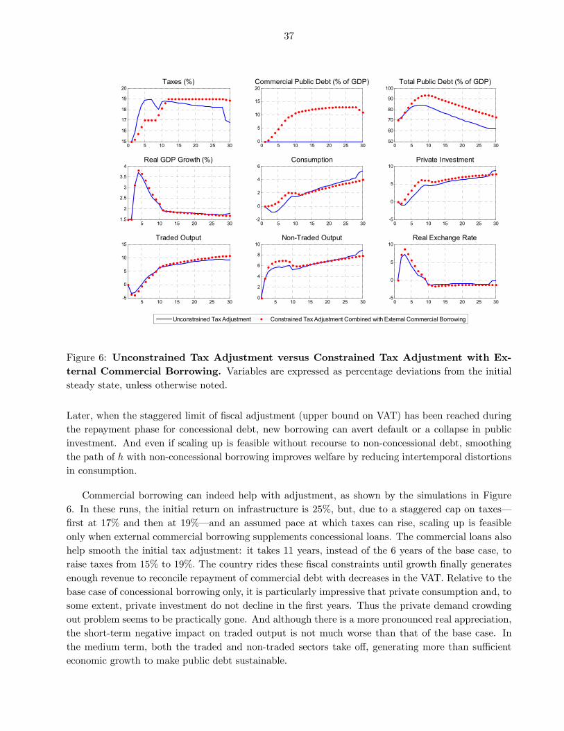
37

0 5 10 15 20 25 3015

16

17

18

19

20Taxes (%)

Unconstrained Tax Adjustment Constrained Tax Adjustment Combined with External Commercial Borrowing

0 5 10 15 20 25 300

5

10

15

20Commercial Public Debt (% of GDP)

0 5 10 15 20 25 3050

60

70

80

90

100Total Public Debt (% of GDP)

5 10 15 20 25 301.5

2

2.5

3

3.5

4Real GDP Growth (%)

0 5 10 15 20 25 30-2

0

2

4

6Consumption

0 5 10 15 20 25 30-5

0

5

10Private Investment

5 10 15 20 25 30-5

0

5

10

15Traded Output

5 10 15 20 25 300

2

4

6

8

10Non-Traded Output

0 5 10 15 20 25 30-5

0

5

10Real Exchange Rate

Figure 6: Unconstrained Tax Adjustment versus Constrained Tax Adjustment with Ex-

ternal Commercial Borrowing. Variables are expressed as percentage deviations from the initial

steady state, unless otherwise noted.

Later, when the staggered limit of fiscal adjustment (upper bound on VAT) has been reached during

the repayment phase for concessional debt, new borrowing can avert default or a collapse in public

investment. And even if scaling up is feasible without recourse to non-concessional debt, smoothing

the path of with non-concessional borrowing improves welfare by reducing intertemporal distortions

in consumption.

Commercial borrowing can indeed help with adjustment, as shown by the simulations in Figure

6. In these runs, the initial return on infrastructure is 25%, but, due to a staggered cap on taxes–

first at 17% and then at 19%–and an assumed pace at which taxes can rise scaling up is feasible

only when external commercial borrowing supplements concessional loans. The commercial loans also

help smooth the initial tax adjustment: it takes 11 years, instead of the 6 years of the base case, to

raise taxes from 15% to 19% The country rides these fiscal constraints until growth finally generates

enough revenue to reconcile repayment of commercial debt with decreases in the VAT. Relative to the

base case of concessional borrowing only, it is particularly impressive that private consumption and, to

some extent, private investment do not decline in the first years. Thus the private demand crowding

out problem seems to be practically gone. And although there is a more pronounced real appreciation,

the short-term negative impact on traded output is not much worse than that of the base case. In

the medium term, both the traded and non-traded sectors take off, generating more than sufficient

economic growth to make public debt sustainable.

38

0 5 10 15 20 25 3015

16

17

18

19

20

21Taxes (%)

Panel A

Slow TaxAdjustment

0 5 10 15 20 25 300

10

20

30

40

50Commercial Public Debt (% of GDP)

Constrained Tax Adjustment Constrained but Slower Tax Adjustment

0 5 10 15 20 25 3070

75

80

85

90

95

100

105

110Total Public Debt (% of GDP)

0 5 10 15 20 25 300

10

20

30

40

50Effective Public Capital

Panel B

LowEfficiency

0 5 10 15 20 25 300

10

20

30

40

50Commercial Public Debt (% of GDP)

Base Case Efficiency Lower Efficiency

0 5 10 15 20 25 3070

75

80

85

90

95

100

105

110Total Public Debt (% of GDP)

Figure 7: Constrained Tax Adjustment with External Commercial Borrowing: Varying

the Structural and Policy Conditions.The transition paths for taxes and debt when the fiscal

adjustment is slower or public investment is very inefficient.

B.2. Debt Blowups: Structural and Policy Conditions

There are also risks, of course, to taking out additional, more expensive debt. If non-concessional

borrowing serves merely to delay the day of reckoning for an unsound investment program, then

the ensuing debt crisis will be more costly and more traumatic than otherwise. If extra credit does

more than facilitate fiscal adjustment, if instead it diminishes fiscal effort too much for too long–

one interpretation of delaying the initial tax adjustment and lowering the values for 1 and 2 in the

reaction function (29)–the country may end up in a debt crisis. Borrowing-on-all-fronts is a high-risk,

high-return strategy. It may greatly enhance the prospects for debt sustainability or lead to spectacular

failure; much depends on the fine details governing debt contracts, the structural conditions of the

economy, the dynamics of growth, and the speed of fiscal adjustment.

Policy makers might overestimate their capacity for fiscal adjustment, finance low-return projects,

misplace the blueprints for reforms to improve governance and the efficiency of public investment, or

repeatedly succumb to the temptation to put off necessary but unpopular tax increases and expenditure

cuts. In this event we get some dreadful results, as exemplified in Figure 7. The run in Panel A

simulates the case when the government delays raising the VAT. Because of this delay, the government

loses the race against time and the debt blows up. In Panel B the government borrows heavily in

39

the commercial market as it pays off its concessional debt, counting on growth in future tax revenues

to ensure debt sustainability. But since public investment is very inefficient ( = 02) little effective

public capital is accumulated, so future revenue gains are too small to stabilize the debt or even to

prevent it from increasing at an accelerating rate. Similar results of explosive debt growth obtain if the

return on public capital, the capacity to collect user fees or the absorptive capacity are low enough.

C. Constrained Tax Adjustment Combined with Domestic Borrowing

Although the DSAs have traditionally focused on the public external public debt, there is broad

agreement that domestic debt plays an important role in overall debt sustainability. The IMF empha-

sizes that better integration of domestic debt into the DSF is critical to early detection of external

debt vulnerability. In a similar vein, UNCTAD (2004) has warned that controlling growth of domestic

debt may prove the main obstacle to debt sustainability in many LICs.

Accordingly, our last financing scenario involves a government that can sell debt in the domestic

market but not in world capital markets. Domestic debt is then determined by the government budget

constraint according to

= I +1 +

1 + −1 − +

1 + −1

1 + −1 + T − − G −N − −1 (43)

whereas the reactions functions described in (27)-(30) with = still determine the path for transfers

and taxes.47 Concessional borrowing follows the same path described in the calibration section and

new domestic loans are fully repaid (target = 02). As before, for expositional purposes, we assume

that all the burden of the fiscal adjustment fall on taxes; so we set T = T in (28), implying T = Tat all times. We also assume that there is a staggered structure for taxes: = 017 initially and then

jumps to = 019

Domestic borrowing is more prone to trigger unsustainable public debt dynamics than external

commercial borrowing. This is for two reasons. Perhaps the most obvious is that domestic loans

are more expensive than other sources of financing. In our calibration, the real interest rate on

domestic loans at the initial steady-state equilibrium is 4 percentage points higher than the rate

paid on external commercial debt.48 Moreover, it rises with more domestic borrowing. The second

reason domestic borrowing is less effective is that it does not provide additional resources from abroad.

Instead of taxing residents to extract the resources necessary to finance the higher public investment,

the government borrows from them. But either way, the resources have to shift to the public sector,

and the scaling up requires a crowding out of private consumption and investment. Thus if rates on

domestic borrowing were the same as on foreign borrowing, the adjustment path would be much more

47Note that this is equivalent to say that taxes and transfers are determined by the reactions functions (27)-(30), where

= and the gap Gap is defined in (23); while the path of domestic debt is determined by equation (24), which is a

different way to express the government budget constraint.48 Interest payments on the internal debt are usually several times larger than interest payments on the external debt,

exceeding 5% in some countries. Barkbu et al. (2008) also note that empirical studies find that rising domestic debt

significantly increases the likelihood of external debt distress.

40

0 5 10 15 20 25 3015

16

17

18

19

20Taxes (%)

External Commercial Borrowing Domestic Borrowing

0 5 10 15 20 25 305

10

15Real Interest Rate (%)

On Domestic Debt

On External Commercial Debt

0 5 10 15 20 25 300

10

20

30

Public Debt (% of GDP)

External Commercial

Domestic

5 10 15 20 25 301.5

2

2.5

3

3.5

4Real GDP Growth (%)

0 5 10 15 20 25 30-2

0

2

4

6Consumption

0 5 10 15 20 25 30-5

0

5

10

15Private Investment

5 10 15 20 25 30-5

0

5

10

15Traded Output

5 10 15 20 25 300

2

4

6

8

10Non-Traded Output

0 5 10 15 20 25 30-5

0

5

10Real Exchange Rate

Figure 8: Constrained Tax Adjustment: Domestic Borrowing versus External Commercial

Borrowing. Variables are expressed as percentage deviations from the initial steady state, unless

otherwise noted.

difficult with domestic borrowing.49

Given the calibration for domestic interest rates and other parameters, domestically-financed in-

vestment scenarios are thus more likely to be explosive. Recall that external commercial borrowing

yields a sustainable trajectory with fiscal reaction functions implying that a 19% cap on the tax rate is

delayed for more than 10 years. In the same scenario financed by domestic borrowing, public domestic

debt explodes. To avoid this, the same changes to assumptions that eased adjustment with commercial

borrowing would work here: a higher rate of return, higher efficiency, higher rate of user fee collec-

tion, a smaller investment scaling up, etc. To compare the macroeconomic dynamics associated with

domestic borrowing to those with external commercial borrowing for nonexplosive scenarios, we now

speed up fiscal adjustment in the domestic borrowing case to ensure debt sustainability. This can be

achieved by raising the parameter 1 of the reaction function (29) from 0.25 to 0.45 and by increasing

the original caps by 05 percentage points. As a result, in Figure 8 taxes go up to 175% by = 5

and to 195% by = 11. We can see the higher interest rates and much higher degree of crowding

out of private consumption and investment. Both combine to increase fiscal pressure and require that

taxes stay at 195% percent for almost two decades.

49This is analogus to a spend-and-don’t-aborb response to aid surges and creates similar macroeconomic challenges,

as analyzed in detail in Berg et al. (2010a)

41

5 10 15 20 25 3070

80

90

100

110Terms of Trade (Base = 100)

Panel A

TOT Shock,Persistence

5 10 15 20 25 3015

16

17

18

19

20

21

22Taxes (%)

5 10 15 20 25 300

10

20

30

40

50Commercial Public Debt (% of GDP)

No Shock Temporary TOT Shock Permanent TOT Shock

5 10 15 20 25 3070

80

90

100

110

120Total Public Debt (% of GDP)

5 10 15 20 25 3070

80

90

100

110Terms of Trade (Base = 100)

Panel B

AdditionalFinancing

5 10 15 20 25 3015

16

17

18

19

20

21

22Taxes (%)

5 10 15 20 25 300

10

20

30

40

50Supplement (% of GDP)

Commercial Debt

Additional Concessional Debt

More Concessional Borrowing Commercial Borrowing

5 10 15 20 25 3070

80

90

100

110

120Total Public Debt (% of GDP)

Figure 9: External TOT Shocks and Risks: Shocks Persistence and Financing Schemes.

The paths of tax and public debt in the context of unexpected TOT shocks, with different degrees

of persistence (temporary versus permanent) and financing sources to supplement concessional loans

(external commercial borrowing versus more concessional borrowing), when tax adjustment is con-

strained

VI. External Shocks and Risks

Our previous analyses have abstracted from the possibility of unexpected exogenous shocks. It is

said, however, that LICs are particularly vulnerable to terms-of-trade shocks, natural disasters shocks,

and other adverse exogenous shocks.50 This is to some extent due to the structural characteristics of

these countries: LICs tend to be more dependent on primary commodities and have a higher exposure

to natural disasters. Furthermore, as LICs become more financially integrated to the rest of the world

by borrowing in capital markets, they will start resembling emerging economies. As such, they will

be subject more frequently to risk premium shocks that affect the volatility of the real interest rate at

which they can borrow.51

We proceed then to investigate the implications for debt sustainability of big unexpected negative

50For a discussion on importance of these external shocks in explaining the instability of output and the macroeconomic

fluctuations in LICs, see Kose and Riezman (2001) and Raddatz (2007) and references therein.51Neumeyer and Perri (2005), Uribe and Yue (2006) and Fernández-Villaverde et al. (2011) discuss how country

risk premia, country spread and the volatility of the real exchange rate, respectively, affect business cycles in emerging

economies.

42

terms-of-trade (TOT) shocks, negative total-factor productivity (TFP) shocks52–as a way to model

natural disaster shocks–and shocks to the risk premium of public commercial debt.53 To model TOT

shocks we assume a decline of 10% in the relative price of exports and an increase of 20% in the

relative price of intermediate inputs which together imply a negative shock of 25% to the TOT

measured as

Negative TFP shocks are just introduced as a simultaneous and equal decrease of

5% in the productivity scale factors and in the technologies (1) and (2); while the risk premium

shock is modelled as a jump in the premium that on impact raises the real interest rate on external

commercial debt from 6% to almost 10% For this last shock we also turn on the mechanism in our

model that allows for a variable government debt risk premium. This is achieved by setting at a

positive value in our specification in equation (22). Following van der Ploeg and Venables (2011) we

assume = 189

In the analysis to follow we focus on the case where external commercial loans close the financing

gap.

In addition, we concentrate on unexpected shocks that hit at the time when the economy is very

vulnerable. We consider that this time is when the total public debt to GDP ratio would have reached

a maximum, if shocks were absent. The relevance of this timing stems from the following reasons. It is

precisely at this point in time when (i) public debt is more likely to breach one of the IMF-WB’s DSF

indicative thresholds or (ii) an unexpected adverse shock is most likely to place, in principle, public

debt on an unsustainable path.54

Three results stand out from our analysis, summarized by the simulations presented in Figures 9

and 10.

First, the persistence of the shock matters for debt sustainability. Panel A of Figure 9 shows the

implications of varying the persistence of an unexpected TOT shock. It is clear that when the shock

is temporary, the country manages a tax adjustment that is sufficient to avoid explosive dynamics for

public commercial debt. Hence public debt is sustainable. But as the persistence of the shock increases,

the debt outcome may become gloomy. If the shock were permanent, the adjustment would become

insufficient, given the caps on taxes. Therefore, if shocks are persistent enough, debt sustainability

52Kraay and Nerhu (2006) find that shocks to real GDP growth are highly significant predictors of debt distress.53Because in our analysis there is perfect foresight, to model unexpected shocks we have to paste two dynamic systems.

Consider, for instance, how to model unexpected TOT shocks. In this case, the first system ignores TOT shocks and

gives us the dynamic paths for all the endogenous variables under the public investment scaling up. This allows us to

retrieve the values of these variables for any particular time when we want to hit the economy with the TOT shock.

Assume that, without loss of generality, this time corresponds to = 9 Then we run a second system that (i) has as

initial conditions for endogenous and exogenous variables the values retrieved from the first system at = 9, (ii) includes

the TOT shocks and (iii) appropriately incorporates the continuation values for the rest of exogenous variables such as

public investment, grants, and concessional borrowing. The final path for each variables is then constructed by pasting

the series of the first system up to = 9 and the series of the second system beyond this point. Note that by our perfect

foresight assumption, this methodology implies that the initial decrease in TOT shocks is the unexpected part. The rest

of the shock, beyond = 9 is still expected. We leave for further work the generalization of this procedure to look at

sequences of unexpected shocks, though because of the perfect foresight assumption, we cannot allow agents to react to

uncertainty per se.54There is nothing, however, that prevents the possibility of explosive debt dynamics if the unexpected shock hits the

economy at any point in the rising path of debt.

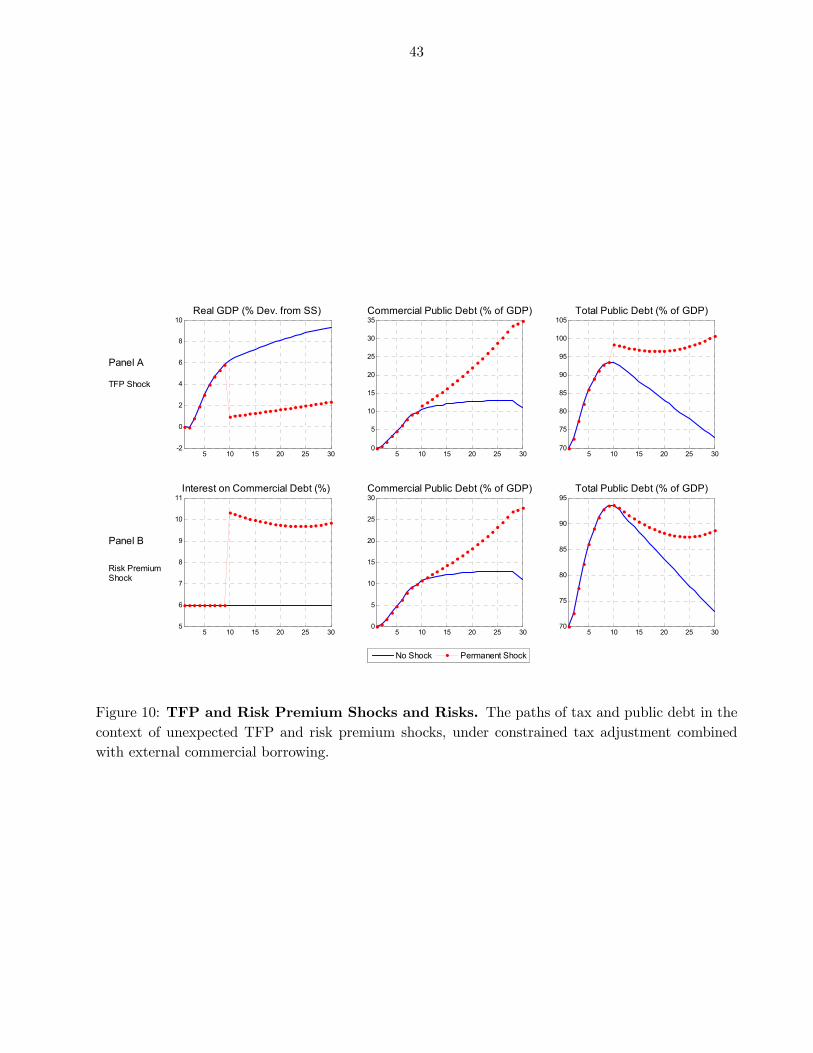
43

5 10 15 20 25 30-2

0

2

4

6

8

10Real GDP (% Dev. from SS)

Panel A

TFP Shock

5 10 15 20 25 300

5

10

15

20

25

30

35Commercial Public Debt (% of GDP)

5 10 15 20 25 3070

75

80

85

90

95

100

105Total Public Debt (% of GDP)

5 10 15 20 25 305

6

7

8

9

10

11Interest on Commercial Debt (%)

Panel B

Risk PremiumShock

5 10 15 20 25 300

5

10

15

20

25

30Commercial Public Debt (% of GDP)

No Shock Permanent Shock

5 10 15 20 25 3070

75

80

85

90

95Total Public Debt (% of GDP)

Figure 10: TFP and Risk Premium Shocks and Risks. The paths of tax and public debt in the

context of unexpected TFP and risk premium shocks, under constrained tax adjustment combined

with external commercial borrowing.

44

problems may easily arise. Of course, this also depends on the magnitude of the shocks and the scale

of additional public investment.

Second, in the context of unexpected shocks, additional concessional financing instead of external

commercial loans could greatly reduce the risks of debt unsustainability. Panel B of Figure 9 shows

that when an unexpected TOT shock hits the economy, additional concessional borrowing to finance

the public investment surge, while setting caps in the tax adjustment, can ensure debt sustainability.

In contrast, using commercial loans may be risky, as unsustainable debt paths become feasible. The

crux of the matter is whether LICs can obtain additional aid in the event of adverse shocks.

Third, unexpected TFP shocks or government debt risk premium shocks can also induce explosive

paths for public debt when the government contracts commercial loans. This is shown in Figure 10

that presents the effects on debt accumulation of permanent negative TFP shocks and government

debt premium shocks. As the reader can easily infer from this figure, similar considerations to those

we raised in the context of TOT shocks–shock persistence and type of additional financing–apply

to these shocks. The risk premium shock case is interesting because it captures the idea that if

market fears of debt repudiation rise and the risk premium rises with the stock of debt, borrowing

and investment programs that were previously sustainable may become unsustainable.55

Summarizing, our analysis of unexpected shocks reveals that the strategy of external commercial

borrowing, although a valuable resource for development, may be risky because it may give rise to

public debt sustainability problems. Size matters here as well: the smaller the scaling up, the larger

the unexpected shock required to cause explosive behavior.

VII. Concluding Remarks

In this paper we have developed a fully-articulated, dynamic macroeconomic model to support

debt sustainability analysis in low-income countries. Our model allows for financing schemes that

mix concessional, external commercial, and domestic debt, while taking into account the impact of

public investment on growth and constraints on the speed and magnitude of fiscal adjustment. In this

regard, our model can help country authorities, IMF country teams, and others build a wide variety of

logically consistent scenarios of public investment surges and other shocks, to inform and complement

the currently used Excel-based DSA. Follow-on work will develop the apparatus to bring the model to

data and conduct DSAs in a build-and -distribute approach.

We calibrate the model to the “average” LIC and provide simulations for a public investment

surge, showing the macroeconomic consequences and potential risks associated with different financing

schemes. We find that when the economy can only borrow concessionally to cover part of the surge,

difficult fiscal and private sector adjustments seem unavoidable in the short to medium term, especially

when the surge is front-loaded and the structural conditions of the economy are weak. The strategy

55A more interesting but much more challenging approach will be to endogenize default in the model and make the

risk premium depend on the model-consistent risk of default.

45

of allowing for external commercial borrowing in LICs may ease these adjustments; but the presence

of weak structural and policy conditions and/or unexpected exogenous shocks calls for caution, as

this strategy is also prone to induce unsustainable public debt dynamics. Domestic borrowing, on

the other hand, is not as effective as external commercial borrowing, because it does not provide

additional external resources, requires more drastic fiscal adjustments, and worsens the crowding out

of the private sector.

The model is already being used to support debt sustainability analysis in country cases.56 These

applications have motivated extensions of the model, including considering external commercial bor-

rowing and domestic borrowing at the same time, modeling regional market borrowing, studying the

implications of financing public investment with natural resource revenues, modeling investment in

security, and financial repression issues, among others.

Still, a number of additional exercises and extensions would be useful. The prospects for debt

sustainability would depend on the composition of public investment, including in human capital.

Our model now assumes that all new public investment is allocated to physical infrastructure projects

with a short gestation period. But even infrastructure can take many years to come on line. And

from a debt sustainability perspective, the distinctive feature of human capital investments is their

long gestation period. Also, user fees finance a much smaller fraction of recurrent costs for education

and health than for power, roads, and water and sanitation. The time profiles for supporting fiscal

adjustment and debt are certain therefore to look very different from the time profiles for investment

in physical infrastructure.

Another important extension will be to more systematically incorporate uncertainty and shocks.

It may be feasible to generalize the method used to analyze specific shocks in Section VI. Stochastic

processes could be assumed for exogenous shocks, to the terms of trade and TFP, for example. Some

elements of parameter uncertainty, e.g., about the rate of return to public investment, might be

explicitly addressed.57

Finally, we have not investigated the trade off between costs and benefits of higher long-run debt

levels. All the scenarios examined here assume debt/GDP returns to initial levels. It is plausible,

however, that by raising the long-run level of debt, a country can forgo some of the long-run benefits

of the investment surge in return for an easier transition. In considering such scenarios, it would be

important to consider the risks associated with carrying a permanently higher debt level.

56The model was used to evaluate the authorities’ public investment scaling-up strategies in Togo in the context of

the debt sustainability analysis. Moreover it was used to carry out counterfactual simulations using the projections of

the macroeconomic framework underlying the standard Excel-based DSA. These simulations provided a useful check on

the plausibility and internal consistency of the projections made in the DSA. See Andrle et al. (2012). The model has

been also applied to Burkina Faso and is being applied to Afghanistan, Cape Verde, Cote d’Ivoire, Ethiopia, Ghana, and

Senegal.57See Clinton et al. (2010) as an example, in a different context.

46

Appendix

A. On Public Investment Efficiency, Rates of Return, and Growth

This Appendix elaborates on the concept of “efficiency” and the closely related concept of the rate

of return to public capital. It serves as background information for the calibration of efficiency and the

rate of return. The bottom line is that the operator needs to be thoughtful when calibrating efficiency,

particularly in considering what it might imply for the marginal product of effective capital. A change

in the calibration of efficiency has two different interpretations: as a level change that applies to the

past and the future, as when comparing two countries at a point in time; or as a change that applies

to future investment but not the past, as for example because of an improvement in public financial

management. It is up to the operator to decide which applies and whether other adjustments to the

calibration are necessary in light of that interpretation.

In the analysis to follow, for simplicity, we assume that there is only one productive sector in the

economy and set the long-run growth rate equal to zero.

“Efficiency” refers to the rate at which spending on public investment translates into public capital.

The model distinguishes between the efficiency of steady-state public investment () and the efficiency

of the additional public investment associated with the surge (). Thus, reproducing equation (20)

from the text with = 0:

= (1− )−1 + ( − ) + (44)

where is public investment (measured in real dollars), is the rate of depreciation of public capital,

= ( + ) is the public investment at the (initial) steady state, and is the stock of “effective”

public capital. It is “effective” because it is what appears in the economy’s production function:

=

¡−1

¢(−1)

()1− (45)

The only nonstandard feature here is that and are not necessarily equal to 1. If they were, then

the usual capital accumulation equation = (1 − )−1 + would obtain. When they are less

than 1, a given rate of public investment results in a smaller accumulation of effective public capital.

What is the effect of additional public investment on growth, and how does it depend on efficiency?

The starting point is that the effect of additional public investment on output–the marginal product

of investment³

−1

´or –depends on both the marginal product of effective public capital–³

−1

´or–and on the efficiency with which public investment spending translates into effective

public capital:

≡

−1=

µ

−1

¶µ−1

−1

¶ (46)

Consider first the marginal product of effective public capital (), which is equal to the rate of

return on effective public capital () plus the depreciation rate . Taking derivatives of the production

function and rearranging terms (and suppressing time subscripts):

≡µ

¶= ()−1 () ()1− =

(47)

47

That is, the marginal product of effective public capital is proportional to the production function

parameter and the output/public capital ratio. The production function embodies decreasing returns

to public capital, holding other factors constant, and given the value of the parameter .

Efficiency has a simple direct effect:

= from equation (44). To understand efficiency, it may

be useful to imagine that all the available public investment projects at a given point in time are ranked

from highest to lowest rate of return. This ranking reflects the decreasing marginal product of public

capital shown in equation (47). The marginal product is thus the return of the best project available. In

a fully efficient investment process, when an additional dollar is spent, this next best project is chosen.

Suppose, though, because of incompetence, corruption, or just imperfect information, a government

chooses worse projects. A lower efficiency–a lower –is a measure of the degree of deviation from the

optimal process. Another–and complementary–way to think about a value of below 1 is simply

that a fraction of spending is literally wasted, e.g. misclassified as investment when it in fact just

covers transfers to civil servants.

It would seem straightforward to obtain the growth impact of public investment. In calibrating

the model, the operator chooses directly a value for the rate of return to effective public capital ,

and thus of the marginal product of public capital. The computer can solve for the implied value of

, given the other parameters of the model. Meanwhile, assumptions about the efficiency parameters

and determine the value of

. These together determine the output effect of additional public

investment from equation (46), holding other factors constant. The other parameters and assumptions

in the model about fiscal policy, private sector behavior, “Dutch disease”, and so on yield the overall

macroeconomic impact of the investment surge.

There is an important potential complication, however: efficiency and the marginal product of

public capital may be related. Whenever–as with the Cobb-Douglas specification of equation (45)–

the marginal product of public capital is declining with larger stocks of public capital, this marginal

product will tend to be higher when efficiency has been low in the past. A country with a low value

of for a given rate of historical or steady-state public investment, will have a low stock of effective

public capital .58 Because the stock of public capital is scarcer, the marginal product of public

capital will tend to be higher. This makes some sense: if a country has difficulty converting spending

into public capital, it will tend to have very little capital, and even a small increment could be highly

productive; think of the first road from the capital city to the port.

In the specific but widely-used case of the Cobb-Douglas production function, which is that used

in the model in the text, the will vary inversely with , and thus with for a given value of .the

production function parameter . In this case, countries with different levels of efficiency will have

the same , holding output, rates of public investment, and other model parameters constant.

Thus, a given increase in public investment spending will have the same effect on output whatever the

value of again given output, rates of public investment, and other model parameters.59

58To see this, it may help to note that, for a case in which = , equation (44) can be solved iteratively to obtain:

= ∞

=1(1− )−, so that is proportional to .

59There is empirical support for declining marginal product of public capital and for the specific Cobb-Douglas version.

Isham and Kaufman (1999) show that the ex post rate of return on World Bank-financed projects (which may correspond

more closely to than ) rises with “good policy” (measured very generally as low inflation, free trade, and

48

This inverse relationship between and has been overridden for the user of the model

because, as was described above, the operator chooses directly. This means that when the

calibration of is changed, the computer finds a different value of as required to preserve the value

of the .60

The upshot is that the operator needs to be thoughtful when calibrating efficiency, particularly in

considering what it might imply for the marginal product of effective capital. In particular, a different

calibration of can be understood in two different ways. It is thus up to the operator to decide which

interpretation applies and whether it calls for other recalibrations:

• According to one interpretation, different calibrations of the value of represent a time-invariantlevel difference in efficiency, e.g. between two countries. Higher steady-state efficiency will imply

a higher marginal product of public investment in the model, because the marginal product of

public capital is given by assumption.61 However, the operator should consider whether this

makes sense in a particular case. How is it that the country wastes less public investment, and

thus presumably has a higher public capital stock, and yet still has the same marginal product

of public capital?

• The second interpretation is that this represents a change in efficiency relative to the past. Sucha change in efficiency through time will have an unambiguous effect on the marginal product of

public investment. This is because it raises the effect of investment spending on the growth rate

of public capital, with no potentially offsetting effect on the size of the stock. Thus, if the idea

is that the country is improving its efficiency relative to its own history, then there is no need

to reflect on possible implications for the marginal product of public capital.

Similar thoughtfulness would seem to apply in the application of the Fund’s policy on non-

concessional borrowing (IMF, 2009b). The policy emphasizes the role of efficiency framed as the capac-

ity to manage public resources well–along with debt levels–in determining whether non-concessional

borrowing for public investment is warranted. But from equation (46), the also matters for the

growth–and hence the debt sustainability–impact of public investment. This may depend on the

broad policy environment and on the scarcity of public capital, and thus could be negatively corre-

lated with steady-state efficiency. Presumably, these considerations need to be brought in through

case-by-case analysis as discussed in the policy.

so on) and falls with the capital/labor ratio. This implies decreasing . Arslanalp et al. (2010) estimate a Cobb-

Douglas production function. They include a further term related to the level of public capital and find a negative

coefficient, consistent with a deviation from Cobb-Douglas in which the falls even faster than implied by Cobb-

Douglas. Servén (2010) provides a direct test in the context of estimated production functions. He finds that the output

elasticity of infrastructure (the percent change in output associated with a given percent change in infrastructure) does

not vary with the stock of infrastructure per worker, supporting a Cobb-Douglas specification.60This approach to calibration can be rationalized with the observation that different measures of policy are positively

correlated: a country that cannot efficiently build an electrical grid probably is not good at keeping it running well. Thus,

countries with low investment efficiency likely also have low marginal product of installed capital, for a given capital

stock (i.e., a relatively low value of ). This offsets the negative effect of higher efficiency on the that operates

through the stock of public capital.61Whether is actually recalibrated does not matter, because the effect of any such change on the marginal product

of investment spending is undone by changes in .

49

References

Adam, C. and D. Bevan, 2006, “Aid and the Supply Side: Public Investment, Export Performance, and Dutch

Disease in Low-Income Countries,” The World Bank Economic Review, Vol. 20(2), pp. 261-290.

Agenor, R. and P. Montiel, 1999, Development Macroeconomics, 2nd edition (Princeton, N.J.; Princeton Uni-

versity Press).

Agenor, R., 2010, “A Thoery of Infrastructure-Led Development,” Journal of Economics Dynamics and Control,

Vol. 34(5), pp. 932-950.

Andrle, M., A. David, R. Espinoza, M. Mills, and L.F. Zanna, 2012, “As You Sow So Shall You Reap: Public

Investment Surges, Growth, and Debt Sustainability in Togo,” IMF Working Paper, forthcoming.

Arestoff, F. and C. Hurlin (2006), “Estimates of Government Net Capital Stocks for 26 Developing Countries,

1970-2002,” World Bank Policy Research Working Paper 3858.

Arslanalp, Serkan Fabian Bornhorst, Sanjeev Gupta, and Elsa Sze, 2010, “Public Capital and Growth”, IMF

Working Paper 10/175 (Washington: International Monetary Fund).

Arnone, M. and A. Presbitero, 2010, Debt Relief Initiatives: Policy Design and Outcomes, forthcoming (Ash-

gate).

Arrow, K., 1962, “The Economic Implications of Learning by Doing.” Review of Economic Studies 29, 153-173.

Asea, P. and C. Reinhart, 1996, “Le Prix de l’Argent: How (Not) to Deal with Capital Flows.” Journal of

African Economies 5 (AERC Supplement), 231-272.

Barkbu, B., C. Beddies, and M. Le Manchec, 2008, “The Debt Sustainability Framework for Low-Income

Countries.” IMF Occasional Paper, No. 266.

Barro, R., 1990, “Government Spending in a Simple Model of Endogenous Growth,” Journal of Political Econ-

omy, Vol. 98(5), pp. S103-26.

Barro, R. and X. Sala-i-Martin, 1992, “Public Finance in Models of Economic Growth,” Review of Economic

Studies, Vol. 59(4), pp. 645-61.

Berg, A., T. Mirzoev, R. Portillo, and L.F. Zanna, 2010a, “The Short-Run Macroeconomics of Aid Inflows:

Understanding the Interaction of Fiscal and Reserve Policy,” IMF Working Paper 10/65.

Berg, A., J. Gottschalk, R. Portillo, and L.F. Zanna, 2010b, “The Macroeconomics of Medium-Term Aid

Scaling-Up Scenarios.” IMF Working Paper 10/160.

Berg, A., R. Portillo, S. Yang, and L.F. Zanna, 2012, “Public Investment in Resource Abundant Low-Income

Countries,” IMF Working Paper, forthcoming .

Blundell, R., 1988, “Consumer Behavior: Theory and Evidence – A Survey.” Economic Journal 98, 16-65.

Blundell, R., P. Pashardes, and G. Weber, 1993, “What do we Learn about Consumer Demand Patterns from

Micro Data?” American Economic Review 83, 570-597.

Briceño-Garmendia, C., K. Smits, and V. Foster, 2008, “Financing Public Infrastructure in Sub-Saharan Africa:

Patterns and Emerging Issues.” AICD Background Paper 15 (World Bank).

Bohn, H., 1998, “The Behavior of US Public Debt and Deficits,” Quarterly Journal of Economics, Vol 113(3),

pp. 949-963.

Calderón, C., E. Moral-Benito, and L. Servén, 2009, “Is Infrastructure Capital Productive? A Dynamic Het-

erogeneous Approach.” Mimeo (World Bank).

50

Calderón, C. and L. Servén, 2010, “Infrastructure in Latin America.” Policy Research Working Paper, No. 5317

(World Bank).

Chatterjee, S. and S. Turnovsky, 2007, “Foreign Aid and Economic Growth: The Role of Flexible Labor Supply,”

Journal of Development Economics, Vol. 84(1), pp. 507—533.

Celasun, O., X. Debrun, and J. D. Ostry, 2007, “Primary Surplus Behavior and Risks to Fiscal Sustainability

in Emerging Market Countries: A ‘Fan-Chart’ Approach,” IMF Staff Papers, Vol. 53(3), pp. 401-425.

Cerra, V., S. Tekin, and S. Turnovsky, 2008, “Foreign Aid and Real Exchange Rate Adjustments in a Financially

Constrained Dependent Economy,” IMF Working Paper 08/204.

Clinton, K., R. Garcia-Saltos, M. Johnson, O. Kamenik, and D. Laxton, 2010, “International Deflation Risks

under Alternative Macroeconomic Policies,” Journal of the Japanese and International Economies, Vol.

24(2), pp. 140-177.

Collier, P., 2007, “The Bottom Billion: Why the Poorest Countries are Failing and What Can Be Done About

It,” Oxford University Press, New York.

Cowan, D., 2010, “Sub-Saharan Africa Macro View.” Citigroup Global Markets.

Dabla-Norris, E., J. Brumby, C. Papageorgiou, A. Kyobe, and Z. Mills, 2011, “Investing in Public Investment:

An Index of Public Investment Management Quality,” IMF Working Paper, 11/37.

Dagher, J., J. Gottschalk, and R. Portillo, 2012, “The Short-run Impact of Oil Windfalls in Low-income Coun-

tries: A DSGE Approach.” Journal of African Economies, forthcoming.

Dalgaard, C. and H. Hansen, 2005, “The Return to Foreign Aid.” Discussion Paper No. 05-04, Institute of

Economics, University of Copenhagen.

Deaton, A., and D. Muellbauer, 1980, Economics and Consumer Behavior (New York, Cambridge University

Press).

Eaton, J., 2002, “The HIPC Initiative: The Goals, Additionality, Eligibility, and Debt Sustainability.” Mimeo

(Operations Evaluation Department, World Bank).

Eberhard, A., V. Foster, C. Bricendo-Garmendia, F. Ouedraogo, D. Camos, and M. Shkaratan, 2008, “Un-

derpowered: The State of the Power Sector in Sub-Saharan Africa.” AICD Background Paper 6 (World

Bank).

Escribano, A., J. Guasch, and J. Pena, 2008, “Impact of Infrastructure Constraints on Firm Productivity in

Africa.” AICD Working Paper No. 9 (World Bank).

EURODAD, 2001, “Putting Poverty Reduction First.” (European Network on Debt and Development)

EURODAD, 2009, “Review of the DSF: Bank & Fund Declare Countries Can Borrow More.” (European Network

on Debt and Development)

Fedelino, A. and A. Kudina, 2003, “Fiscal Sustainability in African HIPC Countries: A Policy Dilemma?” IMF

Working Paper, No. 03/187.

Fernández-Villaverde, J., P. Guerrón-Quintana, J. Rubio-Ramírez, and M. Uribe, 2011. “Risk Matters: The

Real Effects of Volatility Shocks,” American Economic Review, Vol. 101(6), pp. 2530-2561.

Foster, V. and C. Briceño-Garmendia, 2010, Africa’s Infrastructure: A Time for Transformation, forthcoming

(Agence Francaise de Developpement and the World Bank).

Futagami, K., Y. Morita, and A. Shibata, 1993, “Dynamic Analysis of an Endogenous Growth Model with

Public Capital,” Scandinavian Journal of Economics, Vol. 95(4), pp. 607-25.

51

Garcia, M. and R. Rigobon, 2005, “A Risk Management Approach to Emerging Market’s Sovereign Debt Sustain-

ability with an Application to Brazilian Data,” in Inflation Targeting, Debt, and the Brazilian Experience:

1999 to 2003, editors, Francesco Giavazzi, Ilan Goldfajn, and Santiago Herrera, MIT Press.

Ghosh, A., J. Kim, E. Mendoza, J. D. Ostry, and M. Qureshi, 2011. “Fiscal Fatigue, Fiscal Space and Debt

Sustainability in Advanced Economies,” NBER Working Papers 16782, National Bureau of Economic Re-

search.

Glomm, Gerhard and B. Ravikumar, 1994, “Public investment in infrastructure in a simple growth model,”

Journal of Economic Dynamics and Control, Vol. 18(6), pp. 1173-1187.

Greiner, A., 2007, “An Endogenous Growth Model with Public Capital and Sustainable Government Debt,”

The Japanese Economic Review, Vol. 58(3), pp. 345-361.

Greiner, A., W. Semmler, and G. Gong, 2005, The Forces of Economic Growth: A Time Series Perspective, 1st

edition (Princeton, N.J.; Princeton University Press).

Gueye, C. and A. Sy, 2010, “Beyond Aid: How Much Should African Countries Pay to Borrow?” IMF Working

Paper, No. 10/140.

Gupta, S., R. Powell, and Y. Yang, 2006, Macroeconomic Challenges of Scaling Up Aid to Africa: A Checklist

for Practitioners (International Monetary Fund).

Hjertholm, P., 2003, “Theoretical and Empirical Foundations of HIPC Debt Sustainability Targets.” Journal of

Development Studies 39, 67-100.

Hulten, C., 1996, “Infrastructure Capital and Economic Growth: How Well You Use It May Be More Important

Than How Much You Have.” NBER Working Paper, No. 5847.

Hulten, C., E. Bennathan, and S. Srinivasan, 2006, “Infrastructure, Externalities, and Economic Development:

A Study of Indian Manufacturing.” World Bank Economic Review 20, xx-xx.

International Monetary Fund, 2007a, “Regional Economic Outlook: Sub-Saharan Africa,” SM/07/319, available

at http://www.imf.org/external/pubs/ft/reo/2007/afr/eng/sreo1007.pdf

International Monetary Fund, 2007b, “Ghana: Staff Report for the 2007 Article IV Consultation,” SM/07/156,

available at http://www.imf.org/external/pubs/ft/scr/2007/cr07210.pdf

International Monetary Fund, 2009a, “Changing Patterns in Low-Income Country Financing and

Implications for Fund Policies on External Financing and Debt,” SM/09/56, available at

http://www.imf.org/external/np/pp/eng/2009/022509a.pdf

International Monetary Fund, 2009b, “Debt Limits in Fund-Supported Programs: Proposed New Guidelines”,

SM/09/215, available at http://www.imf.org/external/np/pp/eng/2009/080509.pdf

International Monetary Fund, 2010, “Staff Guidance Note on the Application of the Joint Fund-

Bank Debt Sustainability Framework for Low-Income Countries,” SM/10/16, available at

http://www.imf.org/external/np/pp/eng/2010/012210.pdf

International Monetary Fund and World Bank, 2006, “Applying the Debt Sustainablity

Framework for Low-Income Countries: Post-Debt Relief,” SM/06/364, available at

http://www.imf.org/external/np/pp/eng/2006/110606.pdf

International Monetary Fund and World Bank, 2009, “A Review of Some Aspects of

the Low-Income Country Debt Sustainability Framework,” SM/09/216, available at

http://www.imf.org/external/np/pp/eng/2009/080509a.pdf

52

International Monetary Fund and World Bank, 2010, “Preserving Debt Sustainability in

Low-Income Countries in the Wake of the Global Crisis,” SM/10/76 , available at

http://www.imf.org/external/np/pp/eng/2009/080509a.pdf

Isham, Jonathan and Daniel Kaufmann, 1999, “The Forgotten Rationale For Policy Reform: The Productivity

of Investment Projects” Quarterly Journal of Economics, February, Vol. 114, No. 1, pp. 149—184.

Kose, M. A., and R. Riezman, 2001, “Trade Shocks and Macroeconomic Fluctuations in Africa,” Journal of

Development Economics, Vol. 65(1), pp. 55-80.

Kraay, A. and V. Nehru, 2006, “When Is External Debt Sustainable?,” World Bank Economic Review, Vol.

20(3), pp. 341-365.

Lluch, C., A. Powell, and R. Williams, 1977, Patterns in Household Demand and Saving (London, Oxford

University Press).

Mendoza, E. and M. Oviedo, 2004, “Public Debt, Fiscal Solvency and Macroeconomic Uncertainty in Latin

America: The Cases of Brazil, Colombia, Costa Rica, and Mexico,” NBER Working Papers 10637, National

Bureau of Economic Research.

Neumeyer, P., and F. Perri, 2005, “Business Cycles in Emerging Economies: the Role of Interest Rates,” Journal

of Monetary Economics, Vol. 52(2), pp. 345-380.

Ogaki, M., J. Ostry, and C. Reinhart, 1996, ”Saving Behavior in Low- andMiddle-Income Developing Countries.”

IMF Staff Papers 43, 38-71.

Panizza, U., 2008, “Domestic and External Public Debt in Developing Countries.” UNCTAD Discussion Paper,

No. 188.

Perrault, J., L. Savard, and A. Estache, 2010, “The Impact of Infrastructure Spending in Sub-Saharan Africa:

A CGE Modeling Approach.” Policy Research Working Paper, No. 5386 (World Bank).

Pritchett, L., 2000, “The Tyranny of Concepts: CUDIE (Cumulated, Depreciated, Investment Effort) is Not

Capital.” Journal of Economic Growth 5, 361-384.

Raddatz, C., 2007, “Are External Shocks Responsible for the Instability of Output in Low-Income Countries?,”

Journal of Development Economics, Vol. 84(1), pp. 155-187.

Redifer, L., 2010, “New Financing Sources for Africa’s Infrastructure Deficit.” IMF Survey Magazine: Countries

and Regions.

Sachs, J., 2002, “Resolving the Debt Crisis of Low-Income Countries.” Brookings Papers on Economic Activity

1, 257-286.

Schmitt-Grohé, S. and M. Uribe, 2003, “Closing Small Open Economy Models,” Journal of International Eco-

nomics, Vol. 61(1), pp. 163—185.

Servén, Luis, 2010, “Infrastructure investment and growth”, World Bank, in progress; presentation available at

http://www.imf.org/external/np/seminars/eng/2010/spr/lic/index.htm

Steadman Group (2009), “Financial Access Survey for Financial Sector Deepening,” Presentation.

Straub, S., 2008, “Infrastructure and Growth in Developing Countries: Recent Advances and Research Chal-

lenges.” Policy Research Working Paper, No. 4460 (World Bank).

Thurlow, J., D. Evans, and S. Robinson, 2004, “A 2001 Social Accounting Matrix for Zambia.” International

Food Policy Research Institute (Washington, D.C.)

Thurlow, J., X. Diao, and C. McCool, 2008, “2004 Social Accounting Matrix: Malawi.” International Food

Policy Research Institute.

53

Turnovsky, S., 1999, Methods of Macroeconomic Dynamics, 2nd edition (Cambridge, Mass.; MIT Press).

Uribe, M. and V. Yue, 2006, “Country Spreads and Emerging Countries: Who Drives Whom?,” Journal of

International Economics, Vol. 69(1), pp. 6-36.

UNCTAD, 2004, “Analysis of Eligibility and Debt Sustainability Criteria of the HIPC Initiative.” Chapter 2 in

Debt Sustainablility: Oasis or Mirage? (United Nations Conference on Trade and Development).

van der Ploeg, F. and A. Venables, 2011, “Harnessing Windfall Revenues: Optimal Policies for Resource-Rich

Developing Economies,” Economic Journal, Vol. 121(551), pp. 1-30.

Wyplosz, C., 2007, “Debt Sustainability Assessment: The IMF Approach and Alternatives.” HEI Working

Paper, No. 03/2007 (Graduate Institute of International Studies, Geneva).