Public school consolidation: a partial observability spatial

bivariate probit approach

David M. Brasington∗

Department of EconomicsUniversity of CincinnatiCarl H. Lindner Hall

2925 Campus Green DrivePO Box 0371

Cincinnati, OH 45221-0371Phone:513-556-2616Fax:513-556-2669

david.brasington@uc.eduand

Olivier ParentDepartment of EconomicsUniversity of Cincinnatiolivier.parent@uc.edu

Abstract

A pair of municipalities may consolidate services if they are contiguous. Traditionalestimation methods assume that each voting process is independent. Instead we proposea new estimation procedure that allows the probability of consolidation to be influencedby neighboring decisions. We extend a model of local interaction by allowing consol-idation effort of neighbors to be either strategic substitutes or strategic complements.We disentangle direct effects arising from a change in one’s own characteristics fromindirect or spillover effects associated with a change in the other municipalities’ char-acteristics. Results reveal that the endogenous peer effect coming from neighbors is aprimary determinant of willingness to consolidate.

KEYWORDS: social interactions, discrete choice modeling, spatial econometrics,school district consolidation, land annexation.

JEL: C11, C21, H41, H7, I2

∗We would like thank the Taft Research Center, the University Research Council and the research commit-tee of the Carl H. Lindner College of Business of the University of Cincinnati for providing generous researchsupport. The authors acknowledge comments from Chunrong Ai, James P. LeSage, David MacArthur andother participants at the Midwest Econometric Group 2012, NARSC 2011, 2013 and WRSA 2013 confer-ences.

1

1 Introduction

In recent years, economists have paid considerable attention to political integration. Onekey challenge for the empirical literature has been to model the interaction between decisionmakers.

We specify a model where the probability of consolidation for individual pairs of con-tiguous municipalities is influenced by neighboring pairs. For an example at the nationlevel, when West Germany integrated with East Germany in 1990, West Germany becamecontiguous to Poland, which mattered for West Germany’s trade and defense purposes,because Poland was a member of the Warsaw Pact and (unlike East Germany) had foughtagainst Germany in World War II. The new border between a unified Germany and Polandalso allowed for Poland to potentially become a member of NATO in the future. If Poland’sproximity represents peer effects, and these effects are ignored, a model of consolidationwill yield biased parameter estimates. The case we study is school boards. If our schoolboard is considering consolidating with an adjacent school board, and the adjacent schoolboard’s neighbors affect our decision, ignoring the peer effects of those neighbors will leadto biased estimates of the determinants of agreeing to consolidate.

We propose a new estimation procedure based on the spatial Durbin bivariate probitmodel to address the influence of neighboring jurisdictions in a consolidation decision. Tra-ditional attempts to model consolidation involve regressing the number of political units inan urban area (like school districts) as a function of population heterogeneity (e.g., Nelson,1990). Recent studies use probit analysis to model the decision of Connecticut municipalitiesto consolidate public health services (Bates, Lafrancois and Santerre, 2011), and logit analy-sis to model the desire of Norwegian town officials to consolidate their municipality with oneor more neighbors (Sorensen, 2006). Brasington (1999) argues that such approaches fail tomodel the true decision-making involved. The decision to consolidate should be modeled asa joint decision by two specific, contiguous neighboring municipalities. This bivariate probitapproach allows each municipality to decide whether to consolidate with its neighbor, witheach neighbor having veto power. Brasington (2003a, 2003b) extends this approach andlets researchers compare the decision-making of the smaller and larger member of a pair.

Gordon and Knight (2009) introduce a matching algorithm to model consolidation.While they do not allow for multiple member consolidation, they relax the assumption ofindependence in merger decisions of Brasington (1999). The current study extends theapproaches proposed by Brasington (1999) and Gordon and Knight (2009) by allowing theprobability of consolidation between pairs of municipalities to depend on the probability ofconsolidation with their respective neighbors while retaining many of the other attractivefeatures of their models: mutual veto power, multiple member consolidation, and the abilityto separately analyze the decisions of the larger and smaller members of a consolidation. Weextend the model of local interaction of Glaeser and Scheinkman (2001) by allowing the effortof neighboring members of a potential consolidation pair to be either strategic substitutesor strategic complements. We analyze a unique data set of 1,596 pairs of municipalities thatcould potentially consolidate schooling services across 8 urban areas in Ohio and Texas.

The main contribution relies on a simple extension of discrete choice models that wouldallow latent utilities to contain strategic interactions similar to the spatial autoregressiveformulation of the linear-in-means models (as defined in Lee, 2007 and Bramoulle et al.

2

2014 among others) while observing the same stability conditions. This avoids complexcontraction mapping properties to define the rational expectation equilibrium. Estimatesof group interaction might also suffer from the presence of unobservable factors that couldaffect all individual pairs within the same urban area. People typically use traditional fixedeffects approaches, but these require transformations that cannot be implemented in discretechoice models. Instead we invoke the correlated random effects approach (Chamberlin,1984) to model the unobservable factors while avoiding the incidental parameters problem.Another advantage of this approach is that it makes it easy to evaluate partial effectsfor discrete choice models. With spatial dependence, changes in one explanatory variableassociated with one municipality directly affect the willingness to consolidate of the othermember of the pair but are also reflected in the decisions of all other municipalities locatedwithin the same urban area. Our approach makes it feasible to properly interpret the partialderivative impacts from changes in the explanatory variables. Results reveal that local aswell as global interaction effects correspond to a complementarity in consolidation efforts.

The outline of this paper is as follows. Section 2 presents the theoretical framework of thelinear-in-means model. Extension to discrete choice models is provided in Section 3 usingPoirier’s (1980) approach to specify a bivariate model with partial observability. Section 4presents the estimation procedure along with Monte Carlo experiments. We describe thedata in Section 5 while empirical results are discussed in Section 6. Section 7 concludes.

2 Theoretical framework

For the theoretical model, we extend to the bivariate case the traditional social networkmodel recently surveyed in Liu, Patacchini and Zenou (2011), who use network analysis tostudy the impact of peer pressure on adolescents’ sports, education, and video game-playingactivities. Our objective is to probabilistically describe the choice of consolidation of publicschooling provision for a pair i = (1, . . . , n) of neighboring municipalities j = (1, 2).

Let nr be the number of pairs of neighboring municipalities in an urban area r =(1, . . . , r) that could potentially consolidate. Across all urban areas r, the total number ofpairs is equal to n =

∑rr=1 nr. Municipalities are laid out across urban areas, and urban

areas are assumed to be disconnected from each other.1 We describe connections betweenpairs of adjacent municipalities as: Gr = [gil,r], where [gil,r] = 1 if pairs i and l havemunicipalities that are direct neighbors, and [gil,r] = 0 otherwise. Because municipalitiesare either adjacent or not, gil,r = gli,r, which satisfies reciprocity in the networking literature,and, as in the spatial econometric literature, we assume gii,r = 0, that a municipality cannotbe its own neighbor. The data set for our empirical section will be a map of neighboringmunicipalities, some of whom have independent school districts, others of whom have formedconsolidated school districts with one or more neighbors. Taking this map as an equilibrium,we model how the map came to be in this equilibrium as a simultaneous set of decisionsby contiguous pairs of municipalities. We work at the pair level to be able to draw simpleanalogies between the linear-in-means model and the bivariate discrete choice model.

Within each pair i a municipality j = (1, 2) tries to consolidate schooling services with an

1Urban areas like Cincinnati and Dayton are distant from each other and do not share any commonboundary.

3

adjacent municipality (−j) = (1, 2). The two municipalities of that pair i must expend someeffort studying the costs and benefits of consolidating with each other. In our static game,each municipality j = (1, 2) of the pair i in urban area r expends y?ij,r ≥ 0 in consolidationeffort. To better understand how the model is set up, consider the illustration in AppendixA. It shows five political jurisdictions in a metropolitan area. Each jurisdiction can maintainits own school district, or it can consolidate with a willing neighbor. Neighboring pairsare defined as dyads having one municipality in common. Outside the direct consolidationprocess taking place between the two players of that pair i, each of municipality j’s neighborsbelonging to other pairs l also expend a certain amount of effort consolidating with j. Welet yij,r be the average effort of j’s neighbors:

y?ij,r =1

gi,r

nr∑l=1

gil,ry?lj,r, (1)

where gi,r =∑nr

l=1 gil,r is the number of neighboring pairs for individual pair i. Note that asof now the neighboring influence is coming from different pairs but the same order j = (1, 2)of municipality. We will later see that each pair i is composed of a small municipality (j = 1)and large municipality (j = 2) that are contiguous. This equation says that municipalityj’s expectations of the average effort in urban area r equals the average effort of adjacentmunicipalities.

To introduce the bivariate setting, we extend the model of local interaction developedby Glaeser and Scheinkman (2001). Local dependence is based on the interaction betweenboth municipalities j in each pair i and global dependence is based on y?ij,r, the neighborsof municipality j.

Municipality j of pair i chooses its own effort level to maximize utility:

Uij,r(Y?r , Gr) = (aij,r + λr + εij,r)y

?ij,r −

(1− ψ − ϕ)

2y?2ij,r −

ψ

2(y?ij,r − y?i(−j),r)

2 − ϕ

2(y?ij,r − y?ij,r)2 (2)

Certain symbols in Equation (2) require explanation. We let Y ?r = (y?′1,r, . . . , y

?′nr,r)

′

represent the population effort profile in each urban area r with y?1,r = (y?i1,r, y?i2,r)

′. Asin Liu et al. (2011), aij,r represents the idiosyncratic heterogeneity, which is perfectlyobservable by all municipalities. This term captures all the observable characteristics ofthe municipality j (like e.g. enrollment, racial composition, education levels, and propertyvalues etc.) and the average observable characteristics of the neighboring municipalities(contextual effects). In fact, aij,r can be written as:

aij,r = x′ij,rβ2 + (1/gi,r)

nr∑l=1

gil,rx′lj,rγ2 (3)

where xij,r is the Q-dimensional vector of individual-specific characteristics, and β2 and γ2

are parameters of interest.The parameter λr represents unobservable network or urban area characteristics, and

εij,r is an error term, unobservable to the modeler but known to the municipality, whose in-clusion indicates that there is some uncertainty about the benefit of consolidation. The first

4

term of (2) captures the intrinsic utility and reveals that utility depends on a municipality’sown characteristics and the characteristics of its neighbors.

For the pair i, municipality j = (1, 2) must decide whether to consolidate with the othermunicipality (−j) = (1, 2) of that same pair. As in the univariate case intrinsic utility is

defined by a municipality’s own independent effort toward consolidation (1−ψ−ϕ)2 y?2ij,r. The

utility function is strictly concave in own effort as long as ψ + ϕ < 1. In the bivariatecase a municipality’s effort is also a function of the effort of its neighbor. As detailed inBallester et al. (2006), neighboring influences are captured by the cross-derivatives thatare pair-dependent. Following Glaeser and Scheinkman (2001), local interdependence iscaptured by the third term ψ

2 (y?ij,r − y?i(−j),r)2 and depends on the difference between both

municipalities’ effort within each pair i. Negative values for the cross-derivatives (positive ψ)would reveal that consolidation efforts for both members of pair i are strategic substitutes. Ifψ is negative, an increase in municipality (−j)’s consolidation effort would trigger a positiveshift in j’s reaction, allowing effort for both municipalities to be strategic complements.

Global dependence is represented by the last term in (2). It corresponds to the disutilityfor deviating from the group or urban area norms between pairs of potential consolidations.Similar to local dependence, the effort of consolidation with neighboring municipalities ismeasured by the parameter ϕ which also represents a taste for conformity. A negative valuefor ϕ would deter a municipality from merging when its neighbors have a high willingnessto consolidate. A high, positive value would indicate a high taste for conformity in effort,while a low positive value suggests a municipality doesn’t care much about conformingto its neighbors’ consolidation effort. Whether local and global strategic interaction aresubstitutes or complements is theoretically unknown; our empirical section will estimatethe values of those parameters.

The idea is that a municipality cares about its residents and the education of its students.It works to undertake a consolidation with a neighbor if the consolidation benefits residents,but there is a difference between a hostile takeover and a friendly merger. In Ohio and Texas,mutual consent is required for consolidation, but having the two parties agree equally is likelyto provide a more peaceful transition from independent to consolidated school districts.Newspaper articles discuss the poisoned atmosphere of a school district consolidation whereone party was more eager than the other to consolidate.

In addition, the y?ij,r term in (2) implies that the more neighbors a municipality has,the more influences the utility will be averaged over. In general, residents sorting intoan urban area with a large number of municipalities will be able to find a closer matchbetween preferences over taxes, public services, and demographic characteristics, and thusachieve a higher utility, than residents who sort into an urban area with few municipalities.Similarly, the more neighbors a municipality has, the better the chances of a good fit witha neighbor for purposes of school district consolidation. Consolidation is more attractivebetween neighbors with similar size, property values, demographic characteristics and otherunobserved attributes.

Sorting the members of each pair of potential consolidation by size will allow us toidentify separate impacts for the larger and smaller municipality’s neighbors, instead ofestimating an average impact. Previous studies (e.g. Brasington, 2003a) show that thereare differences in how the larger and smaller member of a pair makes its consolidationdecisions, so there might be differences in how the neighbors of the larger and the neighbors

5

of the smaller member of a pair influence consolidation, too.More importantly, within a given urban area, it is hard to disentangle endogenous peer

effects coming from interactions between pairs of municipalities from correlated unobserv-able effects λr associated with similar individual preferences (Moffitt, 2001). In fact, Lee(2007) shows that interaction effects cannot be identified if there is no variation in sizebetween groups or urban areas. He proposes to model unobserved heterogeneity via fixedeffects and discusses efficient estimators to overcome the incidental parameter problem. Be-cause of our interest in identifying marginal effects, we implement the popular correlatedrandom effects model (Chamberlain, 1984). Dependence between the unobserved effectsand explanatory variables is restricted through assumptions on the conditional distributionof heterogeneity given the explanatory variables. Therefore, we do not need to assumeindependence like a traditional random effects model does, and we avoid the incidentalparameters problem as well.

When all pairs of municipalities choose effort level y?ij,r simultaneously to maximize (2),the following first-order conditions result:

δUij,r(Y?r , Gr)

δy?ij,r= aij,r + λr + εij,r − y?ij,r + ψy?i(−j),r + ϕy?ij,r (4)

Using the definition of y?ij,r from (1) along with (4) yields the best-response function:

y?ij,r = ϕ1

gi,r

nr∑l=1

gil,ry?lj,r + (aij,r + λr + εij,r + ψy?i(−j),r)

y?ij,r = ψy?i(−j),r + ϕ1

gi,r

nr∑l=1

gil,ry?lj,r +

x′ij,rβ2 + (1/gi,r)

nr∑l=1

gil,rx′lj,rγ2 + λr + εij,r (5)

For the univariate case, when ψ = 0, Liu, Patacchini and Zenou (2011) show that if|ϕ| < 1 then the game has a unique Nash equilibrium in pure strategies given by (5).By setting specific constraints on ψ and ϕ, Glaeser and Scheinkman (2001) force strategicinteraction to be characterized by efforts that are either complements or substitutes. Thissimplifies tremendously the stability condition of the Nash equilibrium. As discussed inBramoule et al. (2014) in great detail, introducing substitutability into a model of localinteraction effects with complementarity in effort greatly complicates the stability conditionsfor a unique Nash equilibrium. Depending on the magnitude of the minimum eigenvalueof the entire network, multiple equilibria could arise. One crucial difference with Bramouleet al. (2014) is that we allow for both matrices of global and local interactions to berow-normalized. The standard dominance diagonal conditions will ensure the inferiorityand uniqueness of the equilibrium. Stationary regions are defined by the maximum andminimum eigenvalues of the entire network. Maximum eigenvalues for both matrices oflocal and global dependence are equal to one and the largest characteristic root is thusequal to ψ+ϕ. If both parameters are positive, the equilibrium conditions will be satisfiedif ψ + ϕ < 1. When one or both parameters are negative, minimum eigenvalues have to

6

be calculated to define stationary conditions. We will use the complete set of stationaryconditions defined by Elhorst et al. (2012) to ensure the system is stable.

In Ohio and Texas, school boards must each vote in favor for a consolidation to occur,so consolidation involves effort on the part of each school board. The effort of each schoolboard depends on the other’s effort, according to (4) and (5), and these are related decisions.And while the theoretical model has an observed, continuous effort y?, we do not observey?. Instead we observe whether effort is high enough on the part of both parties to resultin a consolidation or not. The measure of effort y?, or willingness to consolidate, thatwe use is the utility differential before and after a potential consolidation. Because theconsolidation process takes place between two municipalities of a same pair i, it argues fora bivariate model. Because we observe consolidation or not, it argues for a probit model.And because we only observe consolidation if both parties vote for it, but we do not observeactual consolidation votes, we have a bivariate probit with partial observability. The spatialcomponent of the bivariate probit model arises from the influence of neighboring pairs - andthe neighbors of the other member of our pair - in the consolidation decision.

Traditionally with discrete choice models, the econometrician only observes the choiceyij,r = m, m ∈ 0, 1 of municipality j that generates the highest utility level. If latentutility were observed by the econometrician, estimating parameters would reduce to linearregression. Using the Bayesian approach, the Data Augmentation step (Tanner and Wong,1987) allows the econometrician to simulate the latent consolidation effort. The idea behinddata augmentation is simply to expand the parameter space with a set of ancillary variablesin order to simplify the estimation of the model.

3 Discrete Choice Modeling

For discrete choice models, the observed choice yij,r depends on the latent utility Uij,r ina non-linear way. As described by Brock and Durlauf (2001) and Tamer (2003) the mainchallenge is that in general, multiple equilibria arise when we try to estimate latent utilitymodels. Lee, Li and Lin (2014) have recently shown that subjective data on expectationsprovides important information in the modeling of social interactions. Using logit and probitmodels, they prove that the existence of an equilibrium is guaranteed only by the fixed pointtheorem, whether the expected probability is constant or heterogeneous across individualsin a group. We model interactions with other individuals in the same group through theirlatent utilities and therefore equilibrium can be achieved with simple properties of stabilityas in the linear-in-means framework, without relying on the fixed point theorem. The mainpurpose of this section is to show that the latent utility difference derived from the bivariateprobit model is equivalent to the Nash equilibrium defined in (5).

Suppose that we no longer observe actual consolidation effort y?ij,r but only whether ornot two municipalities have consolidated yij,r. Following Brock and Durlauf (2001), we setthe observed discrete outcome yij,r = m where m ∈ {−1, 1}. The utility function Uijm,rdeveloped in (2) is now defined with the index m ∈ {−1, 1} and is equivalent to:

Uijm,r(Yr, Gr) = yij,r(aij,r + λr)−ψ

2E(yij,r − y?i(−j),r)

2 −ϕ

2E(yij,r − µij,r)2 + εij,r(yij,r),

7

where µij,r =∑nr

l=1 gil,ry?lj,r denotes the expectation municipality j places on neighboring

consolidation effort. Similar to the linear-in-means model, the penalty terms are expressedas the expected square deviation of j’s consolidation choice from the expected mean effortof others. Then, the willingness to consolidate for municipality j is equivalent to:

Uij1,r(Yr, Gr)− Uij(−1),r(Yr, Gr) = 2(aij,r + λr) + 2ψE(y?i(−j),r) +

2ϕ

nr∑l=1

gil,rE(y?lj,r) + εij,r, (6)

with εij,r = εij,r(1) − εij,r(−1). In this case, equilibrium could be characterized usingthe logistic density and maintaining the i.i.d. error assumptions. Blume et al. (2011)draw an interesting analogy between this binary choice model and the quadratic utilityfunction previously described in the linear-in-means model. Because choice models cannotbe identified, the scalar 2 in front of each term of the willingness to consolidate definedin (6) could be removed. A detailed discussion on identification will be discussed in thissection. We will now show that a similar expression can be obtained using the traditionalsetting yij,r = m where m ∈ {0, 1}, following Poirier (1980).

We consider in an urban area r, a pair i = (1, . . . , n) of neighboring municipalities(j = 1, 2) each faced with the binary choice of consolidation yij,r = m where m ∈ {0, 1}.As in Brasington (2003a), we examine the effect of size in the consolidation decision byimposing j = 1 to be the smaller municipality and j = 2 the larger one. The frameworkcould also be used to split the data by income, race or even to randomly assign pairs.The common formulation of the merger decision between two communities relies on thebivariate probit model. For a given pair i of neighboring communities, vijm,r represents thevector of individual characteristics for municipality j where m ∈ {0, 1} for an urban arear. The bivariate probit model proposed by Poirier (1980) relies on the fact that the twomunicipalities j = 1, 2 have the following utility functions for m ∈ {0, 1}:

Ui1m,r = hi1m(vi1m,r, y?i2,r) + ω1m,r + ηi1m,r

Ui2m,r = hi2m(vi2m,r, y?i1,r) + ω2m,r + ηi2m,r,

where hijm is a scale function, ωjm,r and ηijm,r represent the unobserved attributes.2 Evenif we only observe a single binary outcome of consolidation, the utility maximization frame-work reflects the binary joint choices of two decision-makers’ choices. However, as empha-sized by Gordon and Knight (2009), this model assumes that the consolidation decisionprocess for each pair of neighboring municipalities is independent from all the other poten-tial partners. We extend the bivariate probit model proposed by Poirier (1980) by assumingthat utility for each member in the pair is a function of the member’s willingness to poten-tially consolidate with each of its neighbors. In fact, we want to measure to what extent thedecision process for the consolidation of two municipalities depends on the potential con-solidations neighboring municipalities could undertake. As for the linear-in-means model,we separate the direct influence of the other member of the pair (local effect) from theinfluence of neighboring pairs (global effect). We will show the new latent utility formu-lation is similar to the best reply function defined in (5) and stability conditions remain

2For identification perspective, the parameter expansion technique requires that within each urban arear, small (j = 1) and large (j = 2) municipalities have different fixed effects ωjm,r.

8

identical. For each utility function, we define a new vector Y ?δij

measuring the willingness

to consolidate of all the neighboring communities around a municipality j = (1, 2) of pairi.3 Utility functions are now defined for m ∈ 0, 1 as:

Ui1m,r = hi1m(vi1m,r, y?i2,r, Y

?δi1,r

) + ω1m,r + ηi1m

Ui2m,r = hi2m(vi2m,r, y?i1,r, Y

?δi2,r

) + ω2m,r + ηi2m.

For each pair i, we measure the willingness to consolidate for a municipality j = (1, 2),with the utility differential:

y?ij,r = Uij1,r − Uij0,r.

One way to represent the effect of neighboring decisions is to assume that for a potentialconsolidation pair i, the willingness to consolidate of the smaller community y?i1,r (resp. thelarger, y?i2,r) is first influenced by a set of neighbors δi1 (resp. δi2). The influence ofneighbors on the decision process between two municipalities is modeled using the spatialweight matrix Wj . The elements of the matrix show whether or not two municipalities thatbelong to different pairs are themselves contiguous.4 The coefficients wiljj′ of the (n × n)dimensional matrix Wjj′ , j, j

′ = (1, 2), are equal to one if community j′ of pair i is a neighborof community j belonging to pair l (see Appendix A for further details). The spatial weightis based on the number of neighboring pairs i = (1 . . . , n) that could potentially consolidate.

Thus, we obtain for each municipality j = (1, 2) of the pair i = (1, . . . , n):

hi11(vi11,r, y?i2,r, Y

?δi1

)− hi10(vi10,r, y?i2,r, Y

?δi1

) = ψ1y?2,r + ϕ

nr∑l=1

wil11y?l1,r +

ϕ

nr∑l=1

wil21y?l2,r + xi1,rδ1 (7)

hi21(vi21,r, y?i1,r, Y

?δi2

)− hi20(vi20,r, y?i1,r, Y

?δi2

) = ψ2y?i1,r + ϕ

nr∑l=1

wil22y?l2,r +

ϕ

nr∑l=1

wil12y?l1,r + xi2,rδ2, (8)

where we extended Poirier’s (1980) model for the individual characteristics xij,r to includethe following variables:

xij,r =

[xij,r

nr∑l=1

wil11xl1,r +

nr∑l=1

wil21xl2,r

]. (9)

The first term xij,r of the concatenation (9) is a kj− raw vector of individual characteristicsand the second term is also a kj− raw vector containing the contextual effects obtainedfrom averaging characteristics (with row-normalized spatial weight matrix) of the small(xl1,r) and large (xl2,r) municipalities in neighboring pair l. The 2kj−dimensional vectorδj represents parameters of interest similar to the marginal effects β2 and γ2 defined in the

3Note that this vector excludes the other municipality (−j) of pair i.4The same municipality belonging to two different pairs is not defined as a neighbor.

9

best-reply function (5) of the linear-in-means model. However, unlike the linear-in-meansmodel, Poirier (1980) allows for local interaction to be different between small and thelarge municipalities of each pair. In fact, the effect (ψ1) of the large municipality on thewillingness to consolidate of the small municipality is set to be different from the effect(ψ2) of the small on the large municipality’s willingness to consolidate. Note that thisassumption will be challenged when we investigate identification issues. The parameter ϕmeasures the endogenous effects or the strength of the spatial dependence between neigh-boring municipalities. It corresponds to the same effect measuring the global dependencein the linear-in-means model.

Note that each municipality can be influenced either by a smaller municipality yl1,r ofthe neighboring pair l or by a larger municipality yl2,r. Even though this separation wasnot made in the linear-in-means model, it will help us to identify endogenous effects comingfrom large and small neighboring municipalities. This is a necessary step to analyticallysolve the reduced form developed in Appendix B. This separation forces the unobservedgroup or urban area effects λr to be split between small municipalities (λ1,r) and largemunicipalities (λ2,r)) where ω11,r − ω10,r = λ1,r, ω21,r − ω20,r = λ2,r. We define the newrandom term as ηi11,r − ηi10,r = εi1,r and ηi21,r − ηi20,r = εi2,r.

Let w1ij = (wij11, wij21), w2ij = (wij12, wij22) and Y ?i,r = (y?i1,r, y

?i2,r)

′. Thus for eachpair of municipalities that could consolidate, the spatial bivariate probit model with partialobservability can be rewritten as:

y?i1,r = xi,rβ1 + ρ1

nr∑l=1

w1ilY?l,r + ρ2

nr∑l=1

w2ilY?l,r + µ1,r + νi1,r, (10)

y?i2,r = xi,rβ2 + ρ1

nr∑l=1

w2ilY?l,r + ρ2

nr∑l=1

w1ilY?l,r + µ2,r + νi2,r

where ρ1 = ϕ(1−ψ2)

and ρ2 = ψϕ(1−ψ2)

, by setting ψ1 = ψ2 = ψ. This restriction does not

affect the identification of the marginal effects but simplifies the effect of the neighboringmunicipalities. In fact, the parameter ψ represents the effect of local dependence definedin the linear-in-means model. Because the reduced form involves solving the system withrespect to the local dependence, the global dependence is now characterized by two spatialweight matrices w1ij and w2ij . The decomposition of other marginal effects and unobservedrandom terms are defined in Appendix B. For each pair of potential consolidation the errorterm can be rewritten as: (

νi1,rνi2,r

)iid∼ N

[(00

), R

],

where the correlation matrix R is defined as

R =

(1 %% 1

).

It is important to emphasize that the willingness to consolidate for each communityj = (1, 2) depends on the willingness of its neighbors but also on the neighbors of theother municipality under direct consideration for consolidation. For identification purposes,var(ν1,r) and var(ν2,r) are usually set to one. However we will propose a more flexible

10

specification for the variance matrix that relaxes this constraint and allows for a simplerinterpretation of the estimation results. A discussion about this variance constraint is pro-vided in Appendix C. Identification conditions also require the set of explanatory variablesof the small municipality to be distinct from the large municipality for each pair of potentialconsolidation (see Poirier 1980).5

Note that consolidation only happens if each municipality’s board of education votes infavor of it. The consolidation between two contiguous municipalities fails if one or both ofthe boards votes against it. Because we observe consolidation or no consolidation, instead ofactual consolidation votes by each municipality, we have a situation of partial observability.Partial observability for each potential consolidation i = 1, . . . , n can be modeled using thefollowing random variable:

zi,r = yi1,ryi2,r.

Thus, the likelihood function is:

ln(β1, β2, %, ρ1, ρ2, µ1, µ2) =n∑i

{zi,r lnF (xi,rβ1, xi,rβ2, ρ1, ρ2, µ1, µ2; %)+

(1− zi,r) ln [1− F (xi,rβ1, xi,rβ2, ρ1, ρ2, µ1, µ2; %)]} ,

where F denotes the bivariate standard normal distribution function with correlation coef-ficient % for each of the potential consolidation i = 1, 2, . . . , n.

For estimation purposes, we can rewrite the bivariate expression in matrix form. In fact,for each potential consolidation pair i, we estimate the extent to which the willingness ofmunicipality j = 1 to consolidate with its partner j = 2 is influenced by 1’s own neighborsvia the matrix W1 and by the neighbors of its partner municipality j = 2 via the matrixW2. Each spatial weight Wo, o = (1, 2) is a (2n × 2n)-dimensional matrix, where n is thenumber of potential consolidation pairs. The coefficients of W1 and W2 are defined as:

w1ij =

(wij11 wij21

wij12 wij22

)=

(w1ij

w2ij

), (11)

w2ij =

(wij12 wij22

wij11 wij21

)=

(w2ij

w1ij

). (12)

For matrix form, we set the dependent variable Y ? = (Y ?′1 , . . . , Y

?′n )′ as a vector of

dimension (2n×1). The matrix of explanatory variables X = (X ′1, . . . , X′n)′ is of dimension

(2n × 4K) from which each pair i is defined with the 2K−dimensional vector xi as Xi =(I2 ⊗ xi). The parameters of interest b = (β′1, β

′2)′ are of dimension (4K × 1) and the

2n−dimensional vector of error terms is defined as V = (V ′1 , . . . , V′n)′ with Vi = (νi1, νi2)′.

For each urban area r, the unobserved correlated random effects M = (m′1, . . . ,m′r)′ are of

dimension (2r × 1), with mr = (m1,r,m2,r)′. The (2n × 2r) matrix ∆ serves to impose a

restriction that unobserved heterogeneity is the same for all pairs of municipalities within thesame urban area. The (2n×2r) block diagonal matrix corresponds to ∆ = diag(D1, . . . , Dr)

5The concatenation X with the correlated random effects defined in Appendix D ensures that small andlarge municipalities of the same pair have different values allowing for ψ and ϕ to be identified.

11

where each block is defined as Dr = (ιnr ⊗ I2) with ιnr the nr-dimensional vector of ones.The spatial bivariate probit defined in (10) can now be rewritten in matrix form:

Y ? = Xb+ ρ1W1Y? + ρ2W2Y

? + ∆M + V. (13)

Analyzing stationary conditions, Elhorst et al. (2012) show that |ρ1| + |ρ2| < 1 is toorestrictive. We implement their algorithm to make sure spatial models are always stationary.It is also important to note that by construction, the two spatial weight matrices W1 and W2

are row-normalized and do not have common elements. Even if two municipalities have thesame neighbor, this common neighbor will never be part of the same pair. It is importantto note that the stability conditions remain identical to the linear-in-means model. In fact,if we assume both parameters ρ1 and ρ2 to be positive, then the constraint ρ1 + ρ2 < 1 isequivalent to ϕ

(1−ψ2)+ ψϕ

(1−ψ2)< 1. Those constraints are actually the same as the stability

condition ψ + ϕ < 1 of the Nash equilibrium of the linear-in-means model assuming thatψ and ϕ are positive.6 If either ψ and ϕ are negative, the real minimum eigenvalues of thematrices W1 + (ρ2/ρ1)W2 for each coordinate point located at the border of the stationaryregion (ρ2, ρ1) will have to be determined to establish the system of stationary conditions(see Elhorst et al. 2012).

4 Estimation Method and Monte Carlo Simulations

The estimation is achieved via Markov Chain Monte Carlo (MCMC) methods. LettingB = (I2n−ρ1W1−ρ2W2), the simultaneous spatial autoregressive process can be expressedas:

BY ? = Xb+ ∆M + V. (14)

For Bayesian analysis of this bivariate probit form, we note that the posterior densityis a function of the likelihood and the prior distribution as follows:

p(b,M, ρ1, ρ2,Σ|Y ?, X) ∝ p(Y ?|b,M, ρ1, ρ2,Σ, X)p(b,M, ρ1, ρ2,Σ).

Because direct evaluation of the posterior density is computationally intensive, we useMetropolis-Hastings algorithms to produce a sequence of MCMC samples from the con-ditional posterior distributions for each parameter in the model. The sample of drawsconverges in distribution to a joint posterior for the parameters of our model.

We briefly note some features of our MCMC sampler, with details provided in AppendixD.

To investigate the finite sample performance of our estimator we simulate the followingdata generating process assuming full observability:

Y ? = Xb+ ρ1W1Y? + ρ2W2Y

? + ∆M + V. (15)

V ∼ N(0, In ⊗ Σ)

6It is easy to note that ϕ(1−ψ2)

+ ψϕ(1−ψ2)

< 1⇔ ϕ(1−ψ)

< 1.

12

As detailed in Appendix D, unobserved correlated effects M = (m′1, . . . ,m′r)′ are defined

for the small and large municipalities as mr = (m1,r,m2,r) with mj,r = αj + ¯xj,rκj + µj,rwhere ¯xj,r = 1

nr

∑nri=1(xij,r) represents the average of individual characteristics over each

group r and µr ∼ N(0,Σµ). When running the algorithms, we use prior distributions definedin Appendix D with b0 = 1.01. Pairs of potential consolidation are created by randomlyplacing 250 municipalities. Each municipality faces potential mergers with its neighbors.Pairs are sorted so that the first municipality is the smaller one. We define neighboringmunicipalities using the 5 nearest neighbors. For each dyad, or pair of neighboring munici-palities, the weight matrices W1 and W2 initially have a weight of one if two pairs have onemunicipality in common. The 2n × 2n weight matrix W1 represents the neighboring dyadfor the smaller municipalities whereas W2 represents the neighboring dyad for the largermunicipalities. Both spatial weight matrices are then row normalized.

The sample data are generated with one regressor (k1 = k2 = 1) for each municipalityi, xijr ∼ N(0, 4). For the urban area r, xi1r represents the characteristics for the smallmunicipality and xi2r corresponds to the same variables for the large municipality. In thebivariate setting, the matrix of idiosyncratic heterogeneity for each pair i corresponds toXi = I2 ⊗ [xi1r

∑nrl=1w1ilxl,r xi2r

∑nrl=1w2ilxl,r]. The matrix X = (X ′1, . . . , X

′n)′ is

of dimension 2n × 8. The true parameters are b = ι2 ⊗ (0.5,−0.5, 0.5,−0.5)′, α = (1, 1)′

κ = (2, 2)′, β = (b′, α′, κ′)′, ρ = (0.35, 0.35)′, and

Σ = Σµ =

(1 0.5

0.5 1

). (16)

As in Lee (2007), we consider two situations with 50 groups or urban areas: a casewhere the average size for the urban area is small, and another where it is relatively large.In the first case, the sample size for urban areas varies from 3 to 8 with an average of 5. Inthe large case, the number of urban areas ranges from 15 to 25 with an average of 20 anda sample size of 950. This allows us to analyze the effect of increasing the average groupsize.7 For both cases, we generate 20 replications of 5,000 iterations with a burn-in periodof 4,000 to calculate the posterior means reported in Table (2). Unlike Lee (2007), we donot observe increased bias when groups are larger. In fact, the within group estimatorthat removes the unobserved group fixed effects in Lee (2007) makes the identification of ρdifficult when groups are large. Here we do not suffer from this problem since unobservedeffects are estimated. We also present numerical standard errors (NSE) which give insightinto the accuracy of the Monte Carlo approximation (see Geweke 1991 for a discussion).8

5 Data Description

There are important advantages of our data set over that used in Brasington (1999, 2003a,2003b). First, we add observations from Texas, which not only contributes half our sample:it also allows us to test whether there are differences in how the consolidation decision

7These are the two extreme cases, any situations in between will provide more efficient estimates.8Based on n iterations of the Gibbs sampler, Geweke (1991) proposes estimating the NSE of the sample

mean of the function of interest g(Θ, y) by the square root of its asymptotic variance Sg(O)/N , where Sg(O)is an estimate of the spectral density of the series g(Θ(i), y(i)) (i = l, . . . , S) at frequency zero, and Θ(i) andy(i) are the sampled values.

13

is made in two parts of the U.S.A. that differ in culture and consolidation law. Second,the papers of Brasington (1999, 2003a, 2003b) omit central cities. The argument was thatcentral cities contained heterogeneous populations, while the theoretical model containedinternally homogeneous municipalities. The previous papers also omitted any municipalitythat sent a substantial portion of its population to more than one school district. Ourcurrent study includes central cities and municipalities with split school district assignmentsbecause it takes a much closer look at the data. For example, the City of Houston sends itschildren to sixteen school districts! While it would be easier to omit Houston as having notmade a unified decision about where to send its students, we instead treat each of the sixteenpieces of the City of Houston as a separate municipality. We examine maps to see whichCensus tracts and block groups belong to the portion of the City of Houston that sendsits students to Pasadena School District, and we add up the data from these Census tractsand block groups to find the population, income, racial composition, and all the othervariables of interest for this new Houston City-Pasadena School District “municipality”.The same is true for smaller municipalities like Texas City, whose students attend TexasCity, Dickinson, and Lamarque School Districts. While the data work is much more time-consuming, it allows us to include a larger number of observations. For example, we coverthe same urban areas of Ohio as Brasington (1999) did, but while he had 298 observationsfor Ohio, we have 821.

We draw our sample from the largest urban areas in Ohio and Texas in 2000. Thelegal and geo-political environment for school consolidation across both states is detailedin Appendix E. The Ohio urban areas are Toledo, Cincinnati, Cleveland, Columbus andDayton, which range in population from 670,000 to 2.2 million. In Texas, our sample coversHouston (5.9 million), Dallas (6.4 million), and San Antonio (2.1 million).9 The samplecontains 1596 observations, where an observation is a pair of municipalities that couldpotentially consolidate schooling services or belong to different school districts. Of these1596, Ohio contributes 821 observations and Texas 775. These 1596 observation pairs comefrom 655 municipalities (291 in Texas and 364 in Ohio). There are 227 school districtsin our sample: 101 in Texas and 126 in Ohio. Texas school districts are fewer in numberand larger in size than Ohio’s, probably because Texas has a minimum size of nine squaremiles. This difference in consolidation decisions across both states forced us to separate thedeterminants of consolidation between the states of Ohio and Texas. Parameters capturingendogenous effects stay the same across states.

As explained in the previous section, we examine to what extent the larger commu-nity’s consolidation decisions are different from the smaller community’s decisions. As inBrasington (2003a), we split the sample into larger and smaller municipalities. Sources andsummary statistics are presented in Table 3 and Table 4.

6 Estimation Results

To determine the robustness of the main socioeconomic factors influencing the willingnessto consolidate, we decided to present two models capturing different proxy variables for

9Austin was excluded because it has few municipalities and school districts and would have added fewobservations.

14

racial composition, education, income and property value. For Model 1, we implement thefollowing proxy variables: the percent of Hispanic population, percent of students enrolled ingrades 1-12 who attend private schools, percent of occupied housing units that are occupiedby renters rather than owners, percent of households that are married with own child 0-17 years and property value per pupil. For Model 2, the following proxy variables areconsidered: an index measuring ethnic heterogeneity, percent of persons in municipalityaged 5-17 years who speak English less than “very well”, percentage of persons 25 years orolder in municipality whose highest educational attainment is no more than a high schooldegree, and average income of households. For both models, we generate a single chain oflength 50,000 along with a burn-in period of 10,000 iterations. We use prior distributionsdefined in Appendix D with b0 = 1.01.

Estimation results presented in Table 5 and Table 10 show how the larger and smallermembers of each potential consolidation pair decide whether to consolidate with each other.We observe a significant role for spatial dependence. We consider this one of the mostimportant findings of the paper. As previously detailed, there are two parameters measuringspatial dependence. The parameter estimates for ρ1 = ϕ

(1−ψ2), is about 0.39 for Model 1

and 0.32 for Model 2. Recall that there are two members for each pair of municipalitiesthat could consolidate. The parameter ρ1 suggests that the willingness to consolidate forone member of the pair is influenced by its own neighbors. The theoretical model suggestsalso that each municipality in a potential consolidation pair is affected by the neighborsof the other municipality in the pair. This effect is captured by the parameter ρ2. Thespatial dependence parameter ρ2 = ψϕ

(1−ψ2)for both models is around 0.2. It suggests that

the neighbors of the other member of any pair affect the decision to consolidate. For eachpair of municipalities that could consolidate, the neighbors of both municipalities directlyaffect the willingness to consolidate of the two municipalities in the pair. More importantlythe theoretical model allows us to separate the direct influence of the other member of thepair (local effect) from the influence of neighboring pairs (global effect).

More importantly, from the reduced form of the theoretical model defined in (10) we findthe endogenous peer effects coming from neighboring pairs (ψ = 0.54 for Model 1 ψ = 0.63for Model 2) to be greater than the direct effect coming from the other municipality in eachpair of potential consolidation (ϕ = 0.18 for Model 1 and ϕ = 0.12 for Model 2). This resultconfirms the importance of modeling the influence of neighbors of the other member of ourpair. Traditional bivariate probit models that omit endogenous peer effects will obtainbiased estimates. The other statistic of interest, Σ12, measures the correlation between thetwo decision makers’ decisions. The estimate is to 0.35 for both models suggesting that thedecision process cannot be estimated separately between the larger and smaller member ofeach consolidation pair.

With the presence of local and global interactions, any change of a particular municipal-ity’s characteristics will have multiple impacts. Before discussing those impacts in greaterdetail, marginal effects obtained from the reduced form (13) are presented in Table 5 and Ta-ble 10. Even though we cannot interpret them directly, it is possible to retrieve their initialvalues by observing that b = (β′1, β

′2)′ and β1 = [δ1 ψδ2] /(1− ψ2), β2 = [ψδ1 δ2] /(1− ψ2).

Since ψ has been previously identified, the effects of individual characteristics as well ascontextual effects can now be retrieved from δ1 and δ2 as defined in (9). For instance, inModel 1, the contextual effect of the property values per pupil of the small municipality on

15

its willingness to consolidate is equal to 0.114 (= 0.081/(1− 0.542)).There are many ways to calculate marginal effects. We decide to interpret the model

estimates of the spatial Durbin bivariate probit model in light of the approach proposedby Greene (1996) that is based on the derivatives of Prob [y1 = 1, y2 = 1|x1, x2]. Detailsare provided in Appendix F. With the introduction of spatial dependence, changes in oneexplanatory variable associated with one municipality will directly affect the willingness toconsolidate of the other member of the pair (bivariate model) but will also be reflected inthe decisions of all other municipalities located within the same urban area. As describedin LeSage et al. (2011) the indirect effects, evaluated through cross-partial derivatives,cumulate the spillover effects falling on all other observations, but the magnitude will begreater for neighboring municipalities. The concept of direct and indirect effect is similar tothe one detailed in Bramoulle et al. (2014) and Ballester et al. (2006) where municipalitieswill have a direct effect on some other municipalities through the spatial connectivity matrixW and the indirect effects will depend on higher orders of the matrix W k.

The direct effects capture only the own partial derivatives including the feedback ef-fects. The sum of the direct and indirect effects represents the total effects and reflects thecumulative change in probability of consolidation arising from a change in an explanatoryvariable in a typical municipality. For each urban area r, the cumulation process occursover the nr potential pairs of consolidation. The spatial weight matrix being block diagonal,there will be no spillover impact between urban areas. Since changes are observed for theexplanatory variables of each municipality, each change gives rise to 2nr responses includingour own municipality, the other municipality of the pair as well as all other municipalitiesof the other pairs. We obtain a (2n × 2n) block diagonal matrix of partial derivativesreflecting all responses. To overcome the difficulty of presenting an (2n × 2n) matrix ofpartial derivatives for each explanatory variable, LeSage and Pace (2009) propose the useof average scalar summary measures. LeSage et al. (2011) underline that if explanatoryvariables vary substantially over space, scalar summary measures might not be useful forglobal inferences. Since we only work with urban areas, the variables only vary across alimited geography. Therefore, summary measures for the marginal effects are more glob-ally representative. Table 6, Table 7 and Table 8 show the posterior means of the direct,indirect, and total marginal effects for Model 1, and Table 11, Table 12 and Table 13 showthe same for Model 2. These scalar summary estimates required for proper inference arecalculated during each iteration of the MCMC sampling.

We focus first on the impact of the size of the municipality, as measured by the numberof pupils, on the willingness to consolidate. Because of its importance, pup is the onlyvariable appearing in both models. Across specifications we find consistent results. Smallermunicipalities are more reluctant to consolidate. Analyzing the direct effects in Table 6and Table 11, we observe that in Ohio, the smaller a municipality gets the less temptingare the economies of scale gains of consolidation; the city instead prefers to enjoy completepolitical control over the provision of public schooling. The negative estimates of (−0.002)of pupL for Model 1 and (−0.003) for Model 2 reveal that the small municipality in a pairof potential consolidation is more reluctant to consolidate when the other municipality getslarger. Unlike Brasington (2003a), the effects of the number of pupils on school consolidationis different between larger and smaller municipalities. Table 6 shows that in both Ohio andTexas the large municipality is more willing to consolidate if it has more pupils. The positive

16

estimates of pupL (+0.003) in Ohio and (+0.001) in Texas confirm that the big municipalitycan gain some scale economies without sacrificing political control. This is consistent withthe prediction of Ellingsen’s (1998) theory that large jurisdictions favor consolidating withsmaller cities. A large municipality is more encouraged to consolidate with the smallermunicipality, and the effect is stronger the smaller the small municipality is. Moreover,indirect effects summarized in Table 7 and Table 12 show that the large municipality foreach pair in Ohio will have greater positive spatial spillover impact (+0.007 for Model 1and +0.002 for Model 2) on its larger neighboring municipalities.

The literature consistently shows that property value is a strong driver of the probabilityof consolidation. The current study finds that, the richer the municipality’s school districtis in property value, the less willing it is to consolidate. Any consolidation would dilutethe municipality’s property tax base. Similarly, large Ohio municipalities are less willingto consolidate the more property value they have; and large Texas municipalities are morewilling to consolidate when the smaller municipality of the consolidation has a higher per-pupil property value. For both states, the large municipality has a positive spillover impacton the neighbors of the smaller municipality valpup allS with a value of +0.018 for Ohio and+0.003 for Texas. Spillover effects are important particularly for the smaller municipalityin Ohio for which the total effect of +0.020 in Table 8 is mainly explained by the large+0.016 impact in Table 7 of property value of the neighbors of the larger municipality foreach potential consolidation pair.

Similar arguments can be made analyzing the impact of average household income wherethe small municipality is more willing to consolidate if the large municipality has higherincome (+0.047 for the variable avincL in Texas in Table 11).

Like Alesina et al. (2000), which focused on the impact of population heterogeneity onjurisdictional consolidation, we find that racial composition does affect school consolidationin Ohio and Texas. There is a significant role for Hispanic in influencing consolidationin Ohio and Texas. However Ohio seems more influenced by the presence of Hispanics,despite a much larger presence of Hispanics in Texas than Ohio. For each pair of potentialconsolidation in Ohio, the smaller municipality is less likely to consolidate if the largermunicipality has a larger percentage of Hispanics (−0.011). While there is no significantdirect effect of population heterogeneity leikrace on the consolidation decision we do findnegative spillover effects in Ohio in Table 12. In fact, neighbors of large municipalitiesin Ohio with higher levels of racial heterogeneity decrease the probability of consolidationfor both municipalities of each pair. Indirect effects on smaller municipalities are equal to−0.644 and reach −0.815 on larger municipalities.

Consistently significant in Ohio, the percentage of school-aged children who do notspeak English well (pctbadenglish) does influence the willingness to consolidate. Table 11shows that for large jurisdictions, having a higher percentage of children with poor Englishlanguage skills makes them more willing to consolidate (+0.056). Larger municipalities areless likely to consolidate (-0.060) than smaller (-0.027) when the other municipality of thepair has a higher percentage of school-aged children who do not speak English well.

Having a greater private school market share reduces consolidation effort. Among themost important drivers of private school attendance is the quality of public education avail-able and the ability of residents to afford private schooling. For smaller municipalitiesin Ohio and Texas, having larger enrollment in private schools reduces their effort toward

17

consolidation (−0.003 in Ohio and −0.002 in Texas, from Table 6). For larger Texas munici-palities, private school attendance is positively related to the likelihood of consolidation. Foreach pair of potential consolidation in Texas, we observe positive spillover effects (+0.008for privL in Table 7) between the smaller municipality and the neighbors of the largermunicipality.

The percentage of residents who have no more than a high school degree sometimesinfluences consolidation. Similar to the results for pctbadenglish, municipalities with loweducation levels are more willing to consolidate with their neighbors. This is true for smallmunicipalities in Ohio and Texas, as well as for large Texas municipalities.

Having a high percentage of renters affects the likelihood of consolidation, especially forthe larger Ohio and Texas municipalities. The more renters there are in the small Ohio andTexas municipalities, the less larger municipalities are willing to consolidate schooling withthem.

Family composition is also an important determinant of consolidation. For both Ohioand Texas, the willingness to consolidate will be higher if the potential candidate has ahigher proportion of families married with children and lower if the municipality itselfalready has a high proportion of families married with children.

Finally, it is important to analyze the unobserved effects associated with each urbanarea. Predicted values of correlated random effects defined in Appendix D are reported inTable 9 for Model 1 and Table 14 for Model 2. Estimation results show that despite thehigher number of consolidations we observe in Texas, the smaller municipalities are lesslikely to consolidate. Dallas and Houston in Texas and Toledo in Ohio are the only urbanareas for which both models show a negative willingness to consolidate. The decision toconsolidate schooling services with a neighbor varies across urban areas and further revealsthe reluctance for smaller jurisdictions to do so. Analyzing municipality characteristics andtheir effect on neighboring decisions provides insightful explanations about the main factorsrelated to school district consolidation. However, unobserved heterogeneity is only based onmunicipality characteristics averaged over urban areas, and the variation in the willingnessto consolidate reveals that urban area characteristics might also provide further insights intoschool consolidation. The literature has mainly focused on explaining differences in publicgoods provision and school quality between municipalities but little is known about commonfactors existing at the metropolitan area level. A more coherent regional strategy, operatingat the urban area level, could increase efficiency in public goods provision. For instancedifferent degrees of racial segregation across metropolitan areas could be associated with adifferent willingness to spend on local public goods. Hoxby (2000) analyzes the effects ofschool choice across metropolitan area and shows that public schools are more productivewith greater Tiebout choice among districts.

7 Conclusion

This paper proposes an approach to modeling public school consolidation using a social in-teraction framework allowing for both correlations between alternative consolidation choicesas well as between individuals. We also help model unobserved heterogeneity in the urbanarea in which each municipality is located.

To illustrate this new model, we analyze how municipalities interact in making decisions

18

about consolidation of schooling services. Strategic interaction is key to better understand-ing why some pairs of municipalities have a low probability of consolidation.

To reach these conclusions, we try to clearly identify the peer effects from both thecontextual and unobserved correlated effects. We provide necessary and sufficient conditionsfor identification and propose a specification ensuring the existence of a unique equilibrium.To this end, we extend the most current estimation procedure for bivariate probit modelswith partial observability by introducing a spatial Durbin model with correlated randomeffects. The identification of these effects is of paramount importance for policy purposes.We derive analytical expressions related to partial derivatives measuring how changes invalues of an explanatory variable impacts its own and other municipalities. It allows us todisentangle direct effects coming from a change in one’s own characteristics from indirector spillover effects coming from a change in the other municipalities’ characteristics orwillingness to consolidate.

Based on our theoretical framework in which both municipalities must agree to con-solidate public good provision, differences in size discourage consolidation for the smallermunicipality. In fact, only larger differences in size make big municipalities more willingto consolidate. Since smaller municipalities have veto power, larger differences in size hin-der consolidation. By analyzing the willingness to consolidate between pairs of contiguousmunicipalities, results reveal that the merger decision is directly influenced by neighboringpairs that could consolidate. However the direct influence of the other municipality of thepair is still more important than neighboring merger decisions.

Similar to Alesina et al. (2004) we also find evidence that municipalities avoid hetero-geneity because they do not want to interact with different people, but we also find evidencethat people avoid heterogeneity because of the difficulty of cooperating in the provision oflocal public goods.

References

[1] Alesina, A., Baqir R. and Hoxby C. (2004). “Political jurisdictions in heterogeneouscommunities”,Journal of Political Economy, 112, 348-396.

[2] Anderson, Simon P., Jacob K. Goeree, and Charles A. Hol, (1998). “A TheoreticalAnalysis of Altruism and Decision Error in Public Goods Games.” Journal of PublicEconomics 70, 297-323.

[3] Ballester, Coralio, Antoni Calv-Armengol, and Yves Zenou. 2006. “Who’s Who inNetworks: Wanted: The Key Player.” Econometrica 74 (5): 140317.

[4] Bates, Laurie J., Lafrancois, Becky A. and Santerre, Rexford E. 2011. An empiricalstudy of the consolidation of local public health services in Connecticut. Public Choice147(1-2) p. 107-121.

[5] Barnard, J., McCulloch, R., and Meng, X. (2000), “Modeling Covariance Matricesin Terms of Standard Deviations and Correlations, with Application to Shrinkage,”Statistica Sinica, 10, 1281-1311.

19

[6] Blume, L, W. Brock, S. Durlauf, and Y. Ioannides (2011), “Identification of SocialInteractions,” in J. Benhabib, A. Bisin, and M. Jackson (eds.), Handbook of SocialEconomics, Amsterdam: North-Holland.

[7] Bramoulle, Y., Kranton, R. and M. D’Amours (2014). “Strategic Interactions andNetworks,” American Economic Review (104)3, 898-930.

[8] Brasington, D.M. (1999). “Joint provision of public goods: The consolidation of schooldistricts”, Journal of Public Economics, 73, 373-93.

[9] Brasington, D.M. (2003a). “Size and School District Consolidation: Do Opposites At-tract?”, Economica, 70, 673-690.

[10] Brasington, D. (2003b) Snobbery, Racism, or Mutual Distaste: What Promotes andHinders Cooperation in Local Public-Good Provision? Review of Economics and Statis-tics 85, 874 883.

[11] Brock, William A and Durlauf, Steven N, (2001). “Discrete Choice with Social Inter-actions,” Review of Economic Studies, 68(2), 235-60

[12] Chamberlain, G. (1984), “Panel Data,” in Handbook of Econometrics, Volume 2, ed.Z. Griliches and M.D. Intriligator. Amsterdam: North Holland, 1248-1318.

[13] Chib, S. and Greenberg, E. (1998), “Analysis of Multivariate Probit Models,”Biometrika, 85, 347-361.

[14] Chopin, N. (2011) “Fast simulation of truncated Gaussian distributions”, Statistics andComputing, 21(2), 275-288

[15] Elhorst, J. P., Lacombe, D. J. and Piras, G. (2012), “On model specification and pa-rameter space definitions in higher order spatial econometric models”, Regional Scienceand Urban Economics 42(1), 211-220.

[16] Elligsen T. (1998). “Externalities vs internalities: A model of political integration”.Journal of Public Economics, 68, 251-68.

[17] Geweke, J. (1991) Evaluating the Accuracy of Sampling-Based Approaches to the Cal-culation of Posterior Moments, in Bernardo, J., Berger, J., Dawid, A. and Smith, A.(eds.), Bayesian Statistics 4, pp. 641-649. Oxford: Clarendon Press.

[18] Glaeser, E.L., Scheinkman, J.A., 2001. Measuring social interactions. In: Durlauf, S.N.,Young, H.P. (Eds.), Social Dynamics. Brooking Institute, Washington, DC, pp. 83131.

[19] Gordon, N. and B. Knight. (2009). “A Spatial Merger Estimator with an Applicationto School District Consolidation,” Journal of Public Economics, 93, 752-765.

[20] Greene W. (1996) “Marginal Effects in the Bivariate Probit Model.” Working PaperNo. 96-11, Department of Economics, Stern School of Business, New York University,

[21] Hoxby, C.M. (2000) “Does Competition among Public Schools Benefit Students andTaxpayers?” American Economic Review, 90(5), 1209-38.

20

[22] Imai, K. and van Dyk, D. A. (2005). ”A Bayesian Analysis of the Multinomial ProbitModel Using Marginal Data Augmentation”, Journal of Econometrics 124(2): 311-334.

[23] Lee, L.F. (2007) “Identification and Estimation of Econometric Models with GroupInteractions, Contextual Factors and Fixed Effects,” Journal of Econometrics 140,2,333-374.

[24] Lee, L.F., Li, J. and X. Lin (2014), “Binary Choice Models with Social Network underHeterogeneous Rational Expectations”Review of Economics and Statistics, forthcom-ing.

[25] LeSage, J. and R. K. Pace (2009). An Introduction to Spatial Econometrics, ChapmanHall/CRC Press.

[26] LeSage JP, Pace RK, Lam NSN, Campanella R, Liu X (2011) “New Orleans businessrecovery in the aftermath of Hurricane Katrina”. Journal of Royal Statistics Society A174(4), 10071027

[27] Liu Xiaodong, Eleonora Patacchini and Yves Zenou (2011) ”Peer Effects in Education,Sport, and Screen Activities: Local Aggregate or Local Average?”, working paper.

[28] Liu, J. and Wu, Y. (1999), “Parameter Expansion for Data Augmentation,” Journalof the American Statistical Association, 94, 1264-1274.

[29] Manski, Charles. 2004. ”Measuring Expectations.” Econometrica, 72(5): 1329-1376.

[30] McCulloch, R., Polson, N., and Rossi, P. (2000), “A Bayesian Analysis of the Multi-nomial Probit Model with Fully Identified Parameters,” Journal of Econometrics, 99,173-193.

[31] McCulloch Robert E. and Rossi Peter E. (1994), “An Exact Likelihood Analysis of theMultinomial Probit Model.”, Journal of Econometrics, 64(1-2), 207-40.

[32] Moffitt, R. A. (2001). Policy interventions, low-level equilibria, and social interactions,in S. N. Durlauf and H. P. Young (eds), Social Dynamics, MIT press, Cambridge.

[33] Nelson, M.A., (1990). Decentralization of the Subnational Public Sector: An EmpiricalAnalysis of the Determinants of Local Government Structure in Metropolitan Areas inthe U.S. Southern Economic Journal 57(2), 443-457.

[34] Nobile, A. (2000), “Comment: Bayesian Multinomial Probit Models with a Normal-ization Constraint,” Journal of Econometrics, 99, 335-345.

[35] Poirier, D. (1980). Partial observability in bivariate probit models. Journal of Econo-metrics, 12, 209-17.

[36] Sorensen, Rune J. (2006). Local government consolidations: the impact of politicaltransaction costs. Public Choice 127(1-2) p. 75-95.

21

[37] Talhouk A., A. Doucet, K. Murphy (2012) “Efficient Bayesian Inference for Multivari-ate Probit Models with Sparse Inverse Correlation Matrices”. Journal of Computationaland Graphical Statistics, 21, 739-757;

[38] Tamer, E. (2003), “Incomplete simultaneous discrete response models with multipleequilibria”, Review of Economic Studies 70, 147165.

[39] Tanner,M. A., and Wong,W. H. (1987), “The Calculation of Posterior Distributionsby Data Augmentation” (with discussion), Journal of the American Statistical Associ-ation, 82, 528550.

[40] Texas Education Agency (2013). “Consolidations, Annexations, and Name changes ForTexas Public Schools”, updated 8/13/2013.

Appendix A - Illustration of Consolidation

Figure 1 illustrates a situation of an urban area containing five municipalities. In thisstudy, the arrangement of the data is similar to Brasington (2003a, 2003b). Each munici-pality can maintain its own school district or it can consolidate with a contiguous neighbor.For this illustration only two municipalities decide to consolidate. Therefore, we observefour independent school districts. All pairs of potential consolidation are observed at themunicipality level. Thus the dependent variable would take the value one only for pair sixconnecting municipalities D and E and zero for all other pairs.

The first municipality of each potential matching pair always has the lower numberof pupils. We arrange the data to analyze to what extent smaller and larger communitiesdiffer in their willingness to consolidate. In Figure A.1, the physical size of each municipalityreflects the relative number of pupils.

In Figure 1 only municipalities D and E consolidate. Municipalities B and E are notadjacent. They cannot legally form a consolidated school district with each other; there-fore, there should be no potential consolidation pair observation between B and E directly.However, because D and E consolidate their schools, B may try to join the consolidatedschool district D&E. Municipality B may merge with E, then, but only through the ac-tual consolidated school district. Therefore, potential consolidations are observed between(1) adjacent municipalities or (2) municipalities and adjacent consolidated school districts.Neighboring pairs are defined as dyads having one municipality in common. For instance,for the fourth pair of potential consolidation between municipalities B and D, B is influencedby the willingness to consolidate of two smaller municipalities A and C (via the first andthird pairs, respectively) and one larger E (via the fifth pair) whereas D is only influencedby the larger municipality E (via the sixth pair). Note that the second pair of potentialconsolidation has no direct influence on the fourth pair of consolidation. It is importantto note that each municipality will appear in several pairs, each time revealing a differentwillingness to consolidate.

22

Figure 1: School District Consolidation

Appendix B -Reduced form of Discrete Choice Modeling

The error terms εi,r = (εi1,r, εi2,r) are assumed to follow a standard bivariate normal distri-bution, with correlation parameter %. The correlation between the two disturbances allowsfor interdependence between the utility functions of the two municipalities. Each vote is afunction of the sentiment toward consolidation with other jurisdiction. Thus, (7) and (8)are equivalent to:

y?i1,r = ψ1y?i2,r + ϕ

nr∑l=1

wil11y?l1,r +

ϕ

nr∑l=1

wil21y?l2,r + xi1,rδ1 + λ1,r + εi1,r

y?i2,r = ψ2y?i1,r + ϕ

nr∑l=1

wil22y?l2,r +

ϕ

nr∑l=1

wil12y?l1,r + xi2,rδ2 + λ2,r + εi2,r.

These latent utilities are identical to the best-response functions defined in (5). Fromrandom utility maximization theory, municipality j of pair i will vote in favor of consolida-tion m = 1 if:

yij,r = 1 iff y?ij,r > 0, i.e., Uij1,r > Uij0,r.

23

The reduced form is equivalent to:

y?i1,r = xi,rβ1 +ϕ

(1− ψ1ψ2)

(nr∑l=1

wil11y?l1,r +

nr∑l=1

wil21y?l2,r

)(17)

+ψ1ϕ

(1− ψ1ψ2)

(nr∑l=1

wil22y?l2,r +

nr∑l=1

wil12y?l1,r

)+ µ1,r + νi1,r

y?i2,r = xi,rβ2 +ϕ

(1− ψ1ψ2)

(nr∑l=1

wil22y?l2,r +

nr∑l=1

wil12y?l1,r

)+

ψ2φ

(1− ψ1ψ2)

(nr∑l=1

wil11y?l1,r +

nr∑l=1

wil21y?l2,r

)+ µ2,r + νi2,r

The explanatory variables are based on the concatenation xi,r = [xi1,r xi2,r] of dimension(1×2K), K = k1 +k2 and the parameters of interest βj are of dimension (2K×1). In fact,β1 = [δ1 ψ1δ2] /(1 − ψ1ψ2), β2 = [ψ2δ1 δ2] /(1 − ψ1ψ2), the group or urban area effects arenow defined as µ1,r = (λ1,r+ψ1λ2,r)/(1−ψ1ψ2) and µ2,r = (λ2,r+ψ2λ1,r)/(1−ψ1ψ2) and theerror terms are equal to ν1,r = (ε1,r+ψ1ε2,r)/(1−ψ1ψ2) and ν2,r = (ε2,r+ψ2ε1,r)/(1−ψ1ψ2).

Appendix C - Estimation Procedure

Identifiability

The traditional multivariate probit model assumes that each subject i = (1, . . . , n) hasJ distinct binary responses. Let Y ?

i = (Y ?i1, . . . , Y

?iJ)′ denote the J−dimensional vector

of latent utilities received by subject i and Xij represent 1 × K vectors of explanatoryvariables associated with each response. Assuming that K is the same for all responses,Xi = diag(Xi1 . . . , XiJ). The parameters of interest β = (β′1, . . . , β

′J)′ form a JK×1 vector

of unknown regression coefficients and εi is a J×1 error vector, normally distributed with a0 mean and a J×J variance matrix Σ. The parameters of interest (β,Σ) are not identifiablefrom the observed data (Chib and Greenberg, 1998). There are an infinite number of valuesfor those parameters which yield exactly the same model. In fact, by multiplying both sidesby a positive scalar parameter υ, we obtain

υY ? = υ(Xβ + ε) = X(υβ) + υε

where Y ? = (Y ?′1 , . . . , Y

?′n )′ is the nJ × 1 vector of latent utilities and X = (X ′1, . . . , X

′n)′

the nJ × kJ matrix of explanatory variables. The nJ × 1 vector of observed values Y willnot be affected by this scalar parameter and the likelihood of Y |X,β,Σ will be the same asthat of Y |X, υβ, υ2Σ. The probit model cannot distinguish β and Σ separately. To ensureidentifiability of the model parameters, restrictions need to be imposed on the covariancematrix. Following Imai and Van Dyk (2005), we use the symbols Σ, β and µ to representthe unidentified parameters. Removing the Σ symbol signifies the identified parameters Σ,β and µ.

In the univariate case, the standard solution to this problem is to set the varianceto one. However, defining such a restriction in the bivariate case is more complex. An

24

alternative solution proposed by McCulloch and Rossi (1994) is to ignore the identifiabilityissue and analyze the unidentified model by scaling with the sampling covariance throughthe reduction function R = d−1Σd−1, where d is a diagonal matrix with diagonal elements

di =√

Σii. But extra care must be given to the choice of prior distributions for unidentifiedparameters. McCulloch et al. (2000) propose to work with an identified model by setting thefirst diagonal element of the covariance matrix σ11 = 1. Traditional Wishart distributionsfor covariance can no longer be used: they partition the covariance matrix and impose aspecific prior on the identified parameters, but their algorithm is slower to converge. Forthat reason, Nobile (2000) suggests direct simulation from Wishart distributions conditionalon one element of the diagonal. However, for all these approaches, imposing a normalizationconstraint increases the complexity of interpretation for the parameters and priors.

Alternatively, Chib and Greenberg (1998) restrict the entire identified covariance matrixΣ to be a correlation matrix R. An efficient computational approach has been proposed byTalhouk et al. (2012) to overcome the fact there is no conjugate prior for the correlationmatrices. Following Bernard et al. (2000), they impose a prior on the identified matrixR whose elements follow marginal uniform distributions over the interval [−1, 1]. Thismarginally uniform prior distribution for R is given by:

p(R) ∝ |R|J(J−1)

2−1

(∏i

|Rii|−(J+1)/2)

)(18)

whereRii is the principal submatrix ofR. Even if this distribution is not conjugate, samplingcan be easily obtained from a standard inverse Wishart with degrees of freedom equal toν = J + 1 and then scaled back to a correlation matrix using the variance decomposition(Σ = dRd). For the bivariate specification, we have J = 2 and henceforth we will refer tothe correlation matrix R as the identified matrix Σ.

Parameter Expansion

In many situations, Gibbs sampling methods mix poorly and can be slow to converge. Pa-rameter Expanded Data Augmentation or Marginal Augmentation is a technique introducedby Liu and Wu (1999) to improve convergence by adding an additional parameter.

Assume that a multivariate specification is represented by an nJ × 1 vector of observeddata Y that is incomplete and an nJ × 1 vector Y ? represents its missing parts. Supposewe can identify an hidden parameter υ from the complete data model p(Y, Y ?|θ) where θrepresents the parameter of interest and p(Y, Y ?) is the marginal distribution of the completedata. Then we can generate new latent data W from the transformation of the latent dataY ? induced by the expansion parameter υ. This extension preserves the observed-datamodel: ∫

p(Y,W |θ, υ)dW = p(Y |θ).

The link between the newly generated data W and the missing data Y ? corresponds toa one-to-one differentiable mapping Y ? = tυ(W ). In other words, the working parameter υis identifiable given the observed data and augmented data but cannot be identified giventhe observed data alone. Talhouk et al. (2012) define the mapping function between Y ?

i

and Wi as the diagonal matrix d of the unidentified variance matrix Σ such that the ith

25

element di =√

Σii. They conveniently pick υ = (υ1, . . . , υJ) to be a function of d by takingυi = sii/(2d2

i ) where sii is the ith diagonal element of Σ−1 and di is the ith diagonal elementof d = (d1, . . . , dJ). Talhouk et al. (2012) show that the transformation of the latent datacan be defined as Y ? = tυ(W ) = D−1W where D = In ⊗ d and each element d2

i follows aninverted Gamma distribution:

d2i ∼ IG((J + 1)/2, sii/2)

This function is conveniently chosen so that its combination with the prior of θ = (β,Σ),the transformed likelihood, and the Jacobian, will result in posterior distributions that areeasy to sample from. Using the transformation Σ = dΣd, Barnard et al. (2000) emphasizethat if Σ follows a standard inverse Wishart distribution then Σ is equivalent to:

p(Σ) = p(d,Σ)× |J : Σ→ d,Σ| = p(Σ)p(d|Σ)

where the prior distribution p(Σ) has the attractive property of being marginally uniformfor each element sij on the interval [−1, 1]. As previously stated, the prior distribution forp(d|Σ) is a Gamma distribution whose shape and rate parameters are equal to (J+1)/2 and1, respectively. Therefore, we obtain the desired prior distribution p(d|Σ)p(Σ) by samplingΣ from a standard inverse Wishart and using the transformation Σ = dΣd.

For our bivariate specification defined in (23) below, we need to define a joint prior ond and θ = (β, µ, ρ,Σµ,Σ). We assume that β, ρ, µ, Σµ and Σ are independent a priori sothat p(β, µ,Σ,Σµ, ρ, d) = p(d|Σ)p(Σ)p(β)p(µ)p(ρ)p(Σµ).

As detailed in Talhouk et al. (2012), (β, µ,Σ) are sampled under the expanded datamodel. The transformation on the latent variables is obtained from W = Y ?D whereD = In⊗ d is the expansion parameter with di > 0. Therefore, following the model definedin (23), the expanded likelihood follows:

p(W |β, µ,Σ, ρ, d) ∼ N(B−1(DXβ +D∆µ), B−1(In ⊗ dΣd)B−1′) (19)

where B−1 = (I2n−ρ1W1−ρ2W2)−1. It is important to note that ρ and Σµ can be directlysampled from the non-expanded identified specification. A summary of the algorithm weadopt is presented in Table 1.

Appendix D -Conditional Posterior Distributions

Based on (15), a formal statement of the spatial bivariate probit model with group or urbanarea effects can be written as:

BY ? = Xb+ ∆M + V (20)

M ∼ N(M0, Ir ⊗ Σµ) (21)

V ∼ N(02n, In ⊗ Σ)

with X the (2n×4K) matrix of explanatory variables and b the (4K×1) vector of parametersof interest. Following Chamberlain (1982), correlated random effects M = (m′1, . . . ,m

′r)′

are defined for the small and large municipalities as

mj,r = αj + ¯xj,rκj + µj,r (22)

26

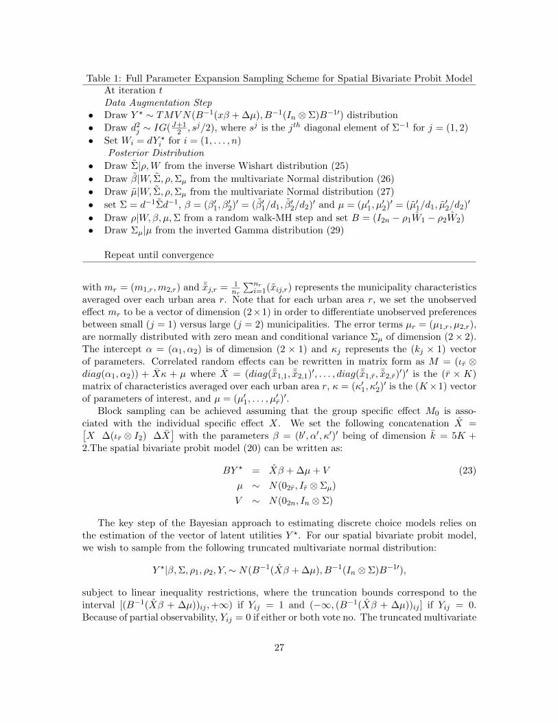
Table 1: Full Parameter Expansion Sampling Scheme for Spatial Bivariate Probit ModelAt iteration tData Augmentation Step

• Draw Y ? ∼ TMVN(B−1(xβ + ∆µ), B−1(In ⊗ Σ)B−1′) distribution

• Draw d2j ∼ IG(J+1

2 , sj/2), where sj is the jth diagonal element of Σ−1 for j = (1, 2)

• Set Wi = dY ?i for i = (1, . . . , n)

Posterior Distribution

• Draw Σ|ρ,W from the inverse Wishart distribution (25)

• Draw β|W, Σ, ρ,Σµ from the multivariate Normal distribution (26)

• Draw µ|W, Σ, ρ,Σµ from the multivariate Normal distribution (27)

• set Σ = d−1Σd−1, β = (β′1, β′2)′ = (β′1/d1, β

′2/d2)′ and µ = (µ′1, µ

′2)′ = (µ′1/d1, µ

′2/d2)′

• Draw ρ|W,β, µ,Σ from a random walk-MH step and set B = (I2n − ρ1W1 − ρ2W2)• Draw Σµ|µ from the inverted Gamma distribution (29)

Repeat until convergence

with mr = (m1,r,m2,r) and ¯xj,r = 1nr

∑nri=1(xij,r) represents the municipality characteristics

averaged over each urban area r. Note that for each urban area r, we set the unobservedeffect mr to be a vector of dimension (2×1) in order to differentiate unobserved preferencesbetween small (j = 1) versus large (j = 2) municipalities. The error terms µr = (µ1,r, µ2,r),are normally distributed with zero mean and conditional variance Σµ of dimension (2× 2).The intercept α = (α1, α2) is of dimension (2 × 1) and κj represents the (kj × 1) vectorof parameters. Correlated random effects can be rewritten in matrix form as M = (ιr ⊗diag(α1, α2)) + Xκ + µ where X = (diag(¯x1,1, ¯x2,1)′, . . . , diag(¯x1,r, ¯x2,r)

′)′ is the (r × K)matrix of characteristics averaged over each urban area r, κ = (κ′1, κ

′2)′ is the (K×1) vector

of parameters of interest, and µ = (µ′1, . . . , µ′r)′.

Block sampling can be achieved assuming that the group specific effect M0 is asso-ciated with the individual specific effect X. We set the following concatenation X =[X ∆(ιr ⊗ I2) ∆X

]with the parameters β = (b′, α′, κ′)′ being of dimension k = 5K +

2.The spatial bivariate probit model (20) can be written as:

BY ? = Xβ + ∆µ+ V (23)

µ ∼ N(02r, Ir ⊗ Σµ)

V ∼ N(02n, In ⊗ Σ)

The key step of the Bayesian approach to estimating discrete choice models relies onthe estimation of the vector of latent utilities Y ?. For our spatial bivariate probit model,we wish to sample from the following truncated multivariate normal distribution:

Y ?|β,Σ, ρ1, ρ2, Y,∼ N(B−1(Xβ + ∆µ), B−1(In ⊗ Σ)B−1′),

subject to linear inequality restrictions, where the truncation bounds correspond to theinterval [(B−1(Xβ + ∆µ))ij ,+∞) if Yij = 1 and (−∞, (B−1(Xβ + ∆µ))ij ] if Yij = 0.Because of partial observability, Yij = 0 if either or both vote no. The truncated multivariate

27

distribution is approximated using the sampling method proposed by Geweke (1991). Thissampler produces an m−step Gibbs iteration procedure based on a series of univariatetruncated Gaussian distributions. For efficiently sampling from these truncated normaldistributions, we implement the simulation procedure proposed by Chopin (2011).

To sample (β, µ,Σ) we adopt the parameter expansion framework defined in (19) usingthe transformation on the latent variables W = Y ?D where D = In⊗d and d = diag(d1, d2)represents the expansion parameter. As previously explained, the working parameter d =diag(d1, d2) is generated from an inverted Gamma distribution d2

i = IG((J + 1)/2, si/2)where the notation si is used to refer to the ith diagonal element of the unidentified matrixΣ−1.

It is important to note that prior distributions for Σ, β and µ have to be the sameunder the observed data model and the expanded model. This is a condition required forthe parameter expansion with marginal augmentation.

As previously explained, using the prior distribution for the correlation matrix Σ definedin (18), Barnard et al. (2000) shows that Σ = dΣd ∼ IW (J+1, IJ) where IW (ν, IJ) denotesthe inverse Wishart distribution defined as:

p(Σ|ν) = |Σ|−(ν+J+1)

2 exp

{−1

2tr(Σ−1)

}. (24)

To reduce correlation between draws, we implement a block sampling scheme and jointlydraw (Σ, β, µ) such that

p(β, µ, Σ|W ) = p(Σ|W )p(β, µ|W, Σ)

then compute the identified parameters using the transformation Σ = d−1Σd−1, β =(β′1, β

′2)′ = (β′1/d1, β

′2/d2)′ and µ = (µ′1, µ

′2)′ = (µ′1/d1, µ

′2/d2)′. To be able to marginal-

ize the conditional distribution of µ over the parameter β we choose a non-informativeuniform prior for β.10

Setting β = (X ′V −1X)−1X ′V −1BW with V = D [(In ⊗ Σ + ∆ (Ir ⊗ Σµ) ∆′]D and µ =

L∆′V −1(BW − Xβ) with L = Λ⊗ (dΣµd) we obtain the following posterior distributions:

Σ|W,ρ ∼ IW (n+ J + 1;

n∑i

U ′i,rUi,r + IJ) (25)

β|Σ,Σµ,W, ρ ∼ N(β, (X ′V −1X)−1), (26)

µ|Σ,Σµ,W, ρ ∼ N(µ,{L− L∆′

[V −1 − V −1X ′(X ′V −1X)−1X ′V −1

]∆L})

, (27)

where Ui,r = Wi,r − ρ1∑n

j w1ijWj,r − ρ2∑n

j w2ijWj,r − Xi,rβ − µr.Unlike the previous estimation step for (Σ,µ,β), the parameters ρ and Σµ are directly

identified. No transformation is required. As noted in LeSage and Pace (2009), the con-ditional posterior distribution for ρj , (j = 1, 2) is not reducible to a standard distribution.A Metropolis-Hastings (MH) step is used to draw from the posterior distribution (28) thatrelies on a random walk proposal with normally distributed increments.

10Unlike the method proposed by McCulloch and Rossi (1994), Imai and van Dyk (2005) underline theflexibility of the parameter expanded scheme in allowing flat priors.

28

Since the posterior distribution for ρj , (j = 1, 2) depends upon its Beta prior p(ρj) =Beta(b0, b0) centered around 0, we obtain:

p(ρj |ρ(−j),Σ,Σµ) ∝ |B|Σ−n/2 exp

(−1

2U ′(In ⊗ Σ−1)U

)p(ρj), (28)

where ρ(−j) is the vector ρj except the jth element and B = (I2n − ρ1W1 − ρ2W2). Theparameter setting for this prior distribution places little weight on the end points of thestationary interval for ρj (see LeSage and Pace (2009) for further discussion).

Finally using an inverted Wishart prior distribution for Σµ ∼ IW (r, IJ), we can simulatethe variance Σµ by reordering the identified correlated random effects in an (r × 2) matrixµ0 = (µ1, µ2) that yields the following posterior distribution:

Σµ ∼ IW(r + J + 1, IJ + µ′0µ0

). (29)

Appendix E - Legal and Geo-Political Environment

In Ohio and Texas, three or more school districts can combine to form a new school dis-trict (Ohio Revised Code 3311.26, Texas Codes 13.151). Princeton City School District inCincinnati has seven municipality members, for example.

In Texas, a consolidation may be initiated by either a resolution of the board of trusteesof the school district or by a petition of registered voters (Texas Codes 13.152), or by thecounty board of education with the consent of the boards of trustees of the school dis-tricts (Texas Revised Statutes 49.12, Article 2740b Section 2). Consolidation may onlytake place between contiguous school districts. Votes occur simultaneously in each affectedschool district, and a majority vote by people in each school district is required for pas-sage. A consolidated school district may be dissolved by the same procedure (Texas Codes13.157(a)), and a new school district may be carved out of an existing school district as longas it is big enough and populous enough (Texas Codes 13.101-13.105). A school district canadd a neighbor if the neighbor votes to abolish itself, too, but consolidation in this mannerstill requires consent by the board of trustees of the receiving school district (Texas Codes13.205(b)).

In addition to consolidation of entire school districts in Texas, territory from a schooldistrict can be detached and annexed to an adjacent school district. The procedures aresimilar to those for consolidation. A school district may be declared dormant by a countycommissioner’s court, and the school district will be annexed to an adjacent school districtupon approval of the receiving board’s trustees. A county commissioner may also force aschool district rated academically unacceptable for two years to be shut down and annexedby a neighboring district or districts, as long as the receiving districts can still meet theireducational and financial obligations to existing students.11 Citizens may also petition tovote that their school district abolish itself. A majority vote carries the motion, but only ifall territory of the abolished school district is annexed to contiguous school districts.

Between the 1983 and 2013 school years in Texas, there have been 35 consolidationsand 27 annexations. Three new school districts formed, including a school district formed

11Receiving school districts get additional state aid.

29

by the detachment of territory from two different school districts. One school district wasannexed to three existing districts. One school district was declared dormant, five districtswere closed or abolished, one school district was forcibly consolidated with a neighbor by thecounty commissioner, and three annexations occurred by order of the county commissioner(Texas Education Agency, 2014).

Ohio consolidation law is similar to that of Texas, except that only school boards caninitiate a vote, and no vote by the people is required, just approval by each pre-consolidationschool board. The procedure for disbanding or splitting up a school district is similar tothe procedure for consolidation (Brasington, 2003b). In Ohio since 1985, three consolidatedschool districts formed, one school district disbanded for lack of students, two school districtsformed from detachment of territory from existing school districts, and three split into theirpre-merger components.

Appendix F - Interpretation of Model Estimates

We extend the method of LeSage and Pace (2011) that produces useful summary measuresof spatial spillover impacts that arise in probit models with a spatial lag in response tochanges in the explanatory variables. For each municipality j of the pair i, the probability ofconsolidation is non-linear in its own as well as in neighboring characteristics. In fact, whenallowing for spatial dependence, changes in the explanatory variables for municipality j inpair i will influence the willingness to consolidate of municipalities belonging to neighboringpairs.

In a simple bivariate probit without endogenous and contextual effects that same changewill only affect the probability of consolidation of both municipalities of the pair i. By settingρ1 = ρ2 = 0 in (10), we can evaluate for a pair i in urban area r the effect on the probabilityof consolidation arising from a change in the kth explanatory variable xki,r = (xki1,r, x

ki2,r),

where xkij,r is the kth explanatory variable of municipality j in pair i. Since xij,r is an

2K−dimensional vector defined in (9), the contextual effects can be removed by constrainingβj,2k = 0, k = 1, . . . ,K.12 Assuming that the change can come from the small or the largemunicipality of each pair, the marginal effect is given as:

δPr(Yi1r = 1, Yi2r = 1|X)

δxki,r= φ(xi1,rβ1 +m1,r)Φ

(xi2,rβ2 +m2,r − %(xi1,rβ1 +m1,r)√

1− %2

)β1,k +

φ(xi2,rβ2 +m2,r)Φ

(xi1,rβ1 +m1,r − %(xi2,rβ2 +m2,r)√

1− %2

)β2,k,

where % is the covariance on the correlation matrix Σ, mj,r are the correlated random effectsdefined in (22), X is the (2n×4K) vector of explanatory variables, β1 is the 2K−dimensionalvector of parameter estimates measuring the effects of small and large municipality char-acteristics on the smaller municipality of each pair and β2 is the 2K−dimensional vectormeasuring the same characteristics on the larger municipality with K = k1 + k2.

In this case, the marginal effect of a change of the 2n−dimensional variable xk on the

12The first K = k1 +k2 elements represents the explanatory variables for the small and large municipalitiesand the second set of K elements represents the contextual effects.

30

probability of consolidation of all pairs is given by:

δPr(Y1 = 1, Y2 = 1|X)

δxk′=

2∑j=1

gjInβj,k, (30)

where gj = φ(ηj)Φ

(η(−j)−%ηj√

1−%2

), with ηj = xjβj + mj and −j represents the other munici-

pality (i.e. η(−j) = η2 if j = 1).For our general model with contextual effects, we simply note that (Inβj,k) has to be

replaced in (30) by (Inβj,k + (W1 + W2)jβj,2k), where (W1 + W2)j represents the (n × n)spatial weight matrix for j = (1, 2).

LeSage et al. (2011) propose a method to analyse the direct and indirect effects in thecase of a spatial autoregressive probit model. Since the small municipalities have a differentspatial weight matrix than the larger municipalities, we rely on the work of Elhorst et al.(2012) who show that it is not possible to dissociate the direct and indirect effects betweenthese two spatial weight matrices.

B−1(ρ1,ρ2) = (I2n − ρ1W1 − ρ2W2)−1 = I2n +

∞∑q=1

(ρ1W1 + ρ2W2)q.

However we can still separate the direct effects based on the diagonal elements of B−1(ρ1,ρ2)

from the indirect effects calculated from the off-diagonal terms of that same matrix B−1(ρ1,ρ2).

Unlike the simple probit model, we observe several non-linear transformations for thepartial derivatives of the bivariate probit because of the presence of the cumulative normaldistribution Φ(.) and its density function φ(.). These non-linearities are reinforced in thespatial case by the presence of the inverse of the spatial weight matrix. In fact, by analyzingthe reduced form of (13), the expected value of the latent variables is equal to Y ? =B−1

(ρ1,ρ2)Xβ +B−1(ρ1,ρ2)M .

Another contrast involves a change in location for observations having different explana-tory variables. It seems impossible to disentangle the impact of a change in location from achange in characteristics. LeSage et al. (2011) argue this can be overcome by the fact thatthe same variables in neighboring locations might have similar values.

For computing marginal effects, we typically use the expression at the sample mean ofthe data but other pertinent values could be analyzed. In the univariate case, LeSage et al.(2011) propose different scalar summary measures that are based on the following (n× n)partial derivatives:

δPr(Y = 1)

δxk′= D [φ(η)]S(ρ)βk

={D [φ(η)] + ρD [φ(η)]W + ρ2D [φ(η)]W 2 + . . .

}βk

where S(ρ) = (In−ρW )−1 = In+ρW+. . .+ρnWn, η = S(ρ)Xβ and d(.) is an n−dimensionalvector of a diagonal matrix D(.).

31

The (n× 1) vector of cumulative total effects is equivalent to:

δPr(Y = 1)

δxk′ιn = D [φ(η)]S(ρ)ιnβk

= D [φ(η)] ιn(1− ρ)−1βk

= d [φ(η)] (1− ρ)−1βk.

The average total effect can be summarized as n−1d [φ(η)]′ ιn(1− ρ)−1βk.And using the diagonal elements, it is easy to obtain the average direct effect:

n−1tr

{δPr(Y = 1)

δxk′

}= {tr(D [φ(η)]) + ρtr(D [φ(η)])W+

ρ2tr(D [φ(η)])W 2 + . . .}βk/n.

We can extend these two summary measures to the bivariate case by replacing η withthe expected value of the latent variables Y ? = B−1

(ρ1,ρ2)Xβ +B−1(ρ1,ρ2)M in (30) and obtain:

(2n)−1ι2nδPr(Y1 = 1, Y2 = 1|X)

δxk′rι′2n = (2n)−1ι2nD [g1β1k + g2β2k]S(ρ1,ρ2)ι2n

= (2n)−1ι2nD [g1β1k + g2β2k] ι2n(1− ρ1 − ρ2)−1

= (2n)−1d [g1β1k + g2β2k]′ ι2n(1− ρ1 − ρ2)−1

(2n)−1tr

{δPr(Y1 = 1, Y2 = 1|X)

δxk′r

}= {tr(D [g1β1k + g2β2k]) + (ρ1 + ρ2)tr(D [g1β1k + g2β2k])W+

(ρ1 + ρ2)2tr(D [g1β1k + g2β2k])W2 + . . .

}βk/(2n).

32

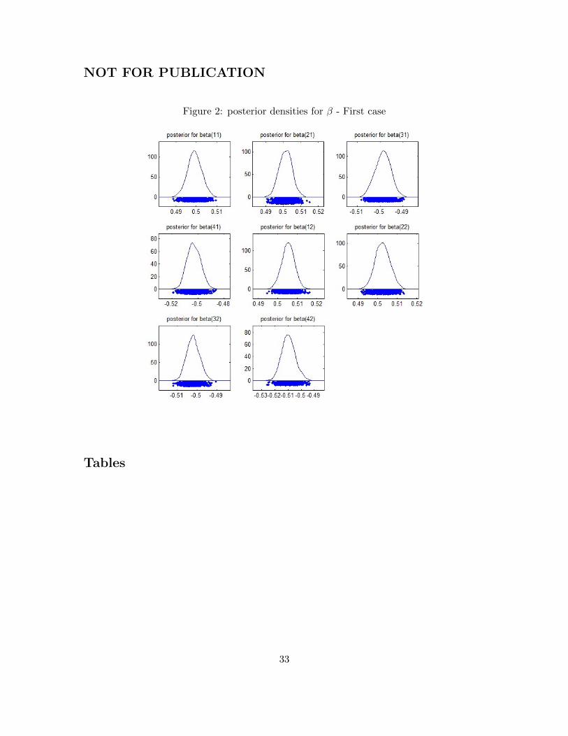
NOT FOR PUBLICATION

Figure 2: posterior densities for β - First case

Tables

33

Figure 3: posterior draws for ρ - First case

Figure 4: posterior draws for σ12 - First case

34

Table 2: Monte Carlo simulations

Parameter True value Mean NSE True value Mean NSE

Small Urban AreasSmall municipalities (j = 1) Large municipalities (j = 2)

ρj 0.35 0.3590 0.0041 0.35 0.3524 0.0032b1j 0.5 0.4857 0.0090 0.5 0.4754 0.0091b2j -0.5 -0.4736 0.0241 -0.5 -0.48456 0.0223b3j 0.5 0.4962 0.0078 0.5 0.4864 0.0075b4j -0.5 -0.4762 0.0255 -0.5 -0.4895 0.0268αj 1 1.0105 0.0085 1 1.0124 0.0088κj 2 2.9806 0.0127 2 2.0306 0.0125σ12 0.5 0.4720 0.0122

Large Urban AreasSmall municipalities (j = 1) Large municipalities (j = 2)

ρj 0.35 0.3519 0.0042 0.35 0.3521 0.0034b1j 0.5 0.4845 0.0084 0.5 0.4871 0.0075b2j -0.5 -0.4815 0.0212 -0.5 -0.4876 0.0245b3j 0.5 0.4892 0.0084 0.5 0.4816 0.0075b4j -0.5 -0.4782 0.0245 -0.5 -0.4812 0.0254αj 1 1.0120 0.0084 1 1.0125 0.0082κj 2 0.9786 0.0115 2 1.97236 0.0119σ12 0.5 0.4880 0.0123

Note: NSE: Numerical Standard Error (see Geweke, 1991)

Table 3: Variable Definition and Sources

Variable Definition Sourcea

pup number of children enrolled in K-12 (public or private) in municipality(in thousands) (1)

renterocc percent of occupied housing units in municipality that are occupied byrenters rather than owners (1)

valpup all property value per pupil; for Ohio it’s class 1 (agricultural and residential)and class 2 (industrial, commercial, mineral, and railroad) real marketvalue of property in dollars divided by number of children enrolled inK-12 (public or private) in municipality; for Texas it’s taxable propertyvalue in dollars divided by number of children enrolled in K-12(public or private) in municipality (in hundreds of thousands) (1),(2),(3)

pctbadenglish percent of persons in municipality aged 5-17 years who speak English lessthan “very well”; p. B-29 of Technical Documentation: Census 2000Summary File 3, U.S. Census Bureau, 2002 (1)

pcthisp percent of municipality population that is Hispanic/Latino/Spanish,and may be of any race (1)

loweduc percentage of persons 25 years or older in municipality whose highesteducational attainment is no more than a high school degreeor equivalent (1)

priv percent of students in municipality enrolled in grades 1-12 who attendprivate schools (1)

avinc average income of households in municipality in tens of thousandsof dollars, where household is householder and other individuals 15+living in household (1)

albundy percent of households in municipality that are married with ownchild 0-17 years (1)

leikrace index created by Robert K. Leik (1966) measure of ethnic heterogeneityin municipality (1)

a: (1) GeoLytics CensusCD 2000 Long Form Release 2.0, East Brunswick, NJ: 2002,(2) “2000 Real Property Abstracts by Taxing District” from Ohio Department of Taxation,(3) Texas Comptroller of Public Accounts, Carole Keeton Strayhorn, Property Tax Division “Annual property tax report tax year 2000appendix D: City local self report data - 2000”

35

Table 4: Variable Mean and Standard Deviation

Ohio TexasSmall Large Small Large

Variable Mean St.Dev. Mean St.Dev. Mean St.Dev. Mean St.Dev.

pup 1.586 1.839 11.130 21.947 2.786 6.600 23.154 48.002renterocc 0.234 0.151 0.274 0.152 0.257 0.199 0.305 0.170valpup all 3.707 3.249 2.778 1.793 8.470 2.364 3.020 5.930

pctbadenglish 1.366 1.670 1.7093 1.4004 5.2521 6.6187 7.5830 6.6912pcthisp 1.287 2.151 1.4937 2.0743 16.5981 17.3016 21.8775 17.6517priv 16.688 14.089 15.8018 9.1368 12.2613 12.5846 8.9517 6.9336

leikrace 0.085 0.075 0.114 0.091 0.348 0.215 0.458 0.243albundy 24.834 7.970 24.478 7.881 30.788 11.145 31.392 8.914loweduc 46.028 18.186 45.374 15.680 39.115 19.400 40.936 17.085avinc 6.470 2.509 6.132 2.156 7.161 3.020 6.537 2.386

Table 5: Estimation Results - Model 1

Parameter Mean s.d. 0.05 0.95 Mean s.d. 0.05 0.95Ohio - Smaller municipalities Ohio - Larger municipalities

pupS -0.040 0.040 -0.104 0.025 -0.023 0.046 -0.095 0.058pupL -0.012 0.005 -0.021 -0.003 -0.012 0.006 -0.021 -0.003valpup allS 0.004 0.048 -0.072 0.084 -0.055 0.042 -0.125 0.016valpup allL -0.073 0.054 -0.166 0.016 -0.136 0.058 -0.236 -0.041albundyS 0.020 0.017 -0.009 0.048 -0.008 0.016 -0.034 0.018albundyL 0.013 0.021 -0.021 0.046 0.003 0.022 -0.036 0.041pcthispS 0.027 0.054 -0.057 0.119 -0.052 0.048 -0.129 0.022pcthispL -0.004 0.055 -0.094 0.091 -0.020 0.065 -0.118 0.091renteroccS 0.006 0.008 -0.008 0.020 -0.004 0.008 -0.017 0.009renteroccL 0.013 0.010 -0.005 0.029 0.004 0.013 -0.017 0.025privS -0.010 0.009 -0.024 0.006 0.010 0.009 -0.004 0.023privL 0.005 0.011 -0.012 0.025 0.023 0.012 0.004 0.045W ∗ pupS 0.001 0.038 -0.065 0.068 -0.021 0.040 -0.086 0.050W ∗ pupL 0.006 0.005 -0.003 0.015 0.010 0.005 0.002 0.019W ∗ valpup allS 0.023 0.033 -0.028 0.081 0.071 0.034 0.021 0.127W ∗ valpup allL 0.081 0.040 0.013 0.148 0.030 0.042 -0.037 0.102W ∗ albundyS -0.005 0.014 -0.029 0.017 0.012 0.014 -0.009 0.038W ∗ albundyL -0.009 0.016 -0.036 0.016 0.003 0.015 -0.022 0.029W ∗ pcthispS -0.026 0.047 -0.109 0.047 0.046 0.042 -0.023 0.110W ∗ pcthispL 0.066 0.043 -0.001 0.142 0.028 0.042 -0.051 0.097W ∗ renteroccS 0.001 0.007 -0.012 0.012 0.009 0.008 -0.002 0.023W ∗ renteroccL -0.007 0.008 -0.021 0.005 -0.001 0.008 -0.013 0.013W ∗ privS -0.005 0.007 -0.018 0.006 -0.010 0.007 -0.022 0.001W ∗ privL -0.005 0.011 -0.022 0.012 -0.017 0.010 -0.034 0.001

Texas - Smaller municipalities Texas - Larger municipalities

pupS 0.027 0.017 -0.002 0.052 0.008 0.013 -0.012 0.029pupL -0.006 0.003 -0.009 -0.002 0.015 0.001 0.012 0.018valpup allS 0.006 0.007 -0.006 0.018 0.002 0.006 -0.008 0.012valpup allL 0.034 0.028 -0.003 0.088 0.004 0.015 -0.019 0.030albundyS -0.033 0.015 -0.057 -0.008 -0.025 0.013 -0.048 -0.004albundyL -0.032 0.019 -0.063 0.002 -0.001 0.019 -0.034 0.032pcthispS -0.016 0.010 -0.034 0.002 0.003 0.009 -0.014 0.018pcthispL 0.001 0.011 -0.016 0.019 0.011 0.014 -0.016 0.032renteroccS -0.013 0.008 -0.028 0.003 -0.006 0.007 -0.019 0.005renteroccL 0.001 0.009 -0.013 0.016 0.001 0.011 -0.016 0.018privS 0.005 0.014 -0.017 0.025 0.010 0.011 -0.008 0.029privL -0.015 0.015 -0.041 0.010 0.028 0.021 -0.006 0.063W ∗ pupS -0.041 0.015 -0.066 -0.016 -0.031 0.013 -0.052 -0.010W ∗ pupL -0.002 0.002 -0.006 0.002 -0.004 0.002 -0.008 0.001W ∗ valpup allS -0.002 0.005 -0.012 0.007 -0.003 0.006 -0.012 0.007W ∗ valpup allL -0.002 0.026 -0.047 0.043 -0.011 0.020 -0.043 0.023W ∗ albundyS 0.041 0.013 0.020 0.062 0.022 0.011 0.001 0.044W ∗ albundyL 0.025 0.009 0.009 0.040 0.005 0.014 -0.017 0.033W ∗ pcthispS 0.002 0.010 -0.014 0.019 -0.006 0.009 -0.021 0.009W ∗ pcthispL 0.018 0.008 0.006 0.033 0.011 0.009 -0.003 0.025W ∗ renteroccS 0.011 0.007 -0.001 0.022 0.010 0.007 -0.001 0.022W ∗ renteroccL 0.002 0.009 -0.012 0.017 -0.007 0.009 -0.020 0.008W ∗ privS -0.007 0.012 -0.028 0.011 -0.011 0.011 -0.029 0.006W ∗ privL 0.015 0.014 -0.009 0.038 -0.018 0.014 -0.041 0.006

Mean s.d. 0.05 0.95ρ1 0.391 0.023 0.347 0.432ρ2 0.213 0.024 0.172 0.254Σ12 0.350 0.074 0.195 0.494

36

Table 6: Estimation Results - Direct effects - Model 1

Parameter Mean s.d. 0.05 0.95 Mean s.d. 0.05 0.95Ohio - Smaller municipalities Ohio - Larger municipalities

pupS 0.007 0.004 -0.001 0.016 -0.009 0.015 -0.038 0.021pupL -0.002 0.001 -0.003 -0.001 0.001 0.001 -0.002 0.001valpup allS -0.009 0.002 -0.013 -0.006 0.003 0.005 -0.008 0.013valpup allL 0.003 0.003 -0.003 0.009 -0.013 0.004 -0.022 -0.005albundyS 0.004 0.003 -0.002 0.009 0.004 0.001 0.002 0.007albundyL -0.001 0.002 -0.005 0.004 -0.005 0.002 -0.009 -0.001pcthispS 0.003 0.005 -0.006 0.013 -0.003 0.001 -0.005 -0.001pcthispL -0.011 0.004 -0.018 -0.003 -0.004 0.008 -0.021 0.012renteroccS 0.001 0.001 -0.001 0.003 -0.002 0.001 -0.004 -0.001renteroccL 0.001 0.001 -0.001 0.003 -0.001 0.001 -0.003 0.001privS -0.003 0.001 -0.005 -0.001 0.001 0.001 -0.002 0.002privL 0.002 0.001 -0.001 0.005 0.002 0.002 -0.001 0.005

Texas - Smaller municipalities Texas - Larger municipalities

pupS -0.002 0.002 -0.005 0.002 -0.010 0.006 -0.021 0.001pupL 0.001 0.001 -0.001 0.001 -0.001 0.001 -0.003 0.001valpup allS 0.001 0.001 -0.001 0.003 0.002 0.001 0.001 0.003valpup allL -0.003 0.003 -0.009 0.002 -0.001 0.002 -0.005 0.003albundyS -0.004 0.002 -0.008 -0.001 -0.003 0.003 -0.009 0.003albundyL 0.004 0.002 0.001 0.008 -0.003 0.003 -0.009 0.004pcthispS -0.001 0.001 -0.003 0.001 -0.002 0.001 -0.003 -0.001pcthispL 0.001 0.001 -0.002 0.002 -0.003 0.002 -0.007 0.001renteroccS 0.002 0.001 0.001 0.003 -0.002 0.001 -0.003 -0.001renteroccL 0.003 0.001 0.001 0.005 0.001 0.002 -0.003 0.003privS -0.002 0.001 -0.004 -0.001 0.005 0.001 0.002 0.007privL 0.002 0.002 -0.002 0.007 0.009 0.004 0.001 0.017

Table 7: Estimation Results - Indirect effects - Model 1

Parameter Mean s.d. 0.05 0.95 Mean s.d. 0.05 0.95Ohio - Smaller municipalities Ohio - Larger municipalities

pupS 0.016 0.008 -0.001 0.033 0.017 0.023 -0.029 0.062pupL 0.001 0.001 -0.001 0.003 0.007 0.001 0.005 0.009valpup allS 0.008 0.002 0.004 0.013 0.018 0.005 0.008 0.028valpup allL 0.016 0.006 0.004 0.029 -0.035 0.017 -0.070 -0.001albundyS 0.004 0.003 -0.002 0.010 0.001 0.003 -0.006 0.007albundyL -0.004 0.004 -0.011 0.003 0.004 0.005 -0.005 0.014pcthispS 0.013 0.010 -0.007 0.033 0.012 0.013 -0.013 0.038pcthispL -0.004 0.014 -0.032 0.023 0.016 0.011 -0.006 0.038renteroccS -0.003 0.001 -0.004 -0.002 0.003 0.002 -0.001 0.007renteroccL 0.001 0.002 -0.003 0.004 -0.001 0.002 -0.006 0.003privS -0.002 0.001 -0.004 0.001 -0.001 0.002 -0.004 0.002privL -0.001 0.003 -0.007 0.005 0.003 0.003 -0.002 0.009

Texas - Smaller municipalities Texas - Larger municipalities

pupS -0.008 0.005 -0.017 0.001 -0.019 0.013 -0.046 0.007pupL 0.001 0.001 -0.001 0.002 0.001 0.001 -0.001 0.002valpup allS 0.002 0.002 -0.002 0.005 0.003 0.001 0.001 0.005valpup allL -0.017 0.010 -0.037 0.004 0.001 0.006 -0.012 0.013albundyS 0.006 0.002 0.001 0.010 0.002 0.003 -0.004 0.008albundyL 0.001 0.003 -0.005 0.007 -0.011 0.008 -0.027 0.004pcthispS -0.001 0.002 -0.005 0.002 -0.002 0.001 -0.005 0.001pcthispL 0.001 0.002 -0.003 0.004 -0.003 0.003 -0.009 0.002renteroccS -0.001 0.001 -0.003 0.002 -0.001 0.001 -0.004 0.002renteroccL 0.005 0.003 -0.001 0.011 0.001 0.003 -0.007 0.006privS -0.004 0.002 -0.009 0.001 -0.005 0.004 -0.013 0.002privL 0.008 0.004 0.001 0.015 0.012 0.006 0.001 0.023

37

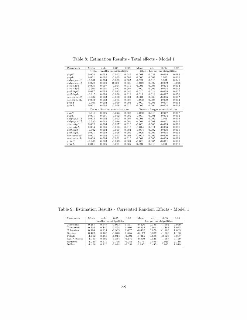
Table 8: Estimation Results - Total effects - Model 1

Parameter Mean s.d. 0.05 0.95 Mean s.d. 0.05 0.95Ohio - Smaller municipalities Ohio - Larger municipalities

pupS 0.024 0.013 -0.002 0.049 0.008 0.038 -0.068 0.083pupL 0.001 0.002 -0.003 0.002 0.006 0.002 0.003 0.010valpup allS -0.001 0.004 -0.009 0.007 0.021 0.010 0.001 0.041valpup allL 0.020 0.010 0.001 0.038 -0.049 0.022 -0.092 -0.006albundyS 0.008 0.007 -0.004 0.019 0.005 0.005 -0.004 0.014albundyL -0.004 0.007 -0.017 0.007 -0.001 0.007 -0.014 0.012pcthispS 0.017 0.015 -0.013 0.046 0.010 0.014 -0.018 0.037pcthispL -0.015 0.018 -0.050 0.019 0.012 0.019 -0.027 0.050renteroccS -0.002 0.003 -0.006 0.001 0.001 0.003 -0.005 0.007renteroccL 0.002 0.003 -0.005 0.007 -0.002 0.004 -0.009 0.004privS -0.004 0.002 -0.009 0.001 -0.001 0.003 -0.007 0.004privL 0.001 0.005 -0.008 0.010 0.005 0.004 -0.004 0.014

Texas - Smaller municipalities Texas - Larger municipalities

pupS -0.010 0.006 -0.023 0.003 -0.030 0.019 -0.067 0.007pupL 0.001 0.001 -0.002 0.002 -0.001 0.001 -0.004 0.002valpup allS 0.003 0.002 -0.002 0.007 0.004 0.002 0.001 0.008valpup allL -0.020 0.013 -0.046 0.005 0.001 0.008 -0.017 0.016albundyS 0.002 0.004 -0.007 0.010 -0.001 0.006 -0.013 0.010albundyL 0.004 0.006 -0.008 0.015 -0.014 0.011 -0.036 0.008pcthispS -0.002 0.003 -0.007 0.004 -0.004 0.002 -0.008 0.001pcthispL 0.001 0.003 -0.006 0.006 -0.006 0.004 -0.015 0.002renteroccS 0.001 0.002 -0.003 0.004 -0.003 0.002 -0.006 0.001renteroccL 0.008 0.004 -0.001 0.016 0.001 0.005 -0.009 0.009privS -0.006 0.003 -0.013 0.001 -0.001 0.005 -0.011 0.009privL 0.011 0.006 -0.001 0.022 0.021 0.010 0.001 0.040

Table 9: Estimation Results - Correlated Random Effects - Model 1

Parameter Mean s.d. 0.05 0.95 Mean s.d. 0.05 0.95Smaller municipalities Larger municipalities

Cleveland 0.267 0.747 -0.963 1.531 -0.226 0.785 -1.602 0.999Cincinnati 0.536 0.840 -0.864 1.910 -0.355 0.901 -1.883 1.043Colombus 0.368 0.814 -0.903 1.637 -0.402 0.879 -1.900 1.003Dayton 0.422 0.765 -0.840 1.625 -0.172 0.807 -1.560 1.133Toledo -1.002 0.456 -1.914 -0.091 -1.215 0.688 -2.628 0.007San Antonio -1.785 0.802 -3.384 -0.176 -0.899 0.536 -1.967 0.169Houston -1.235 0.579 -2.398 -0.081 1.075 0.495 0.025 2.110Dallas -1.466 0.716 -2.894 -0.031 0.995 0.485 0.045 1.919

38

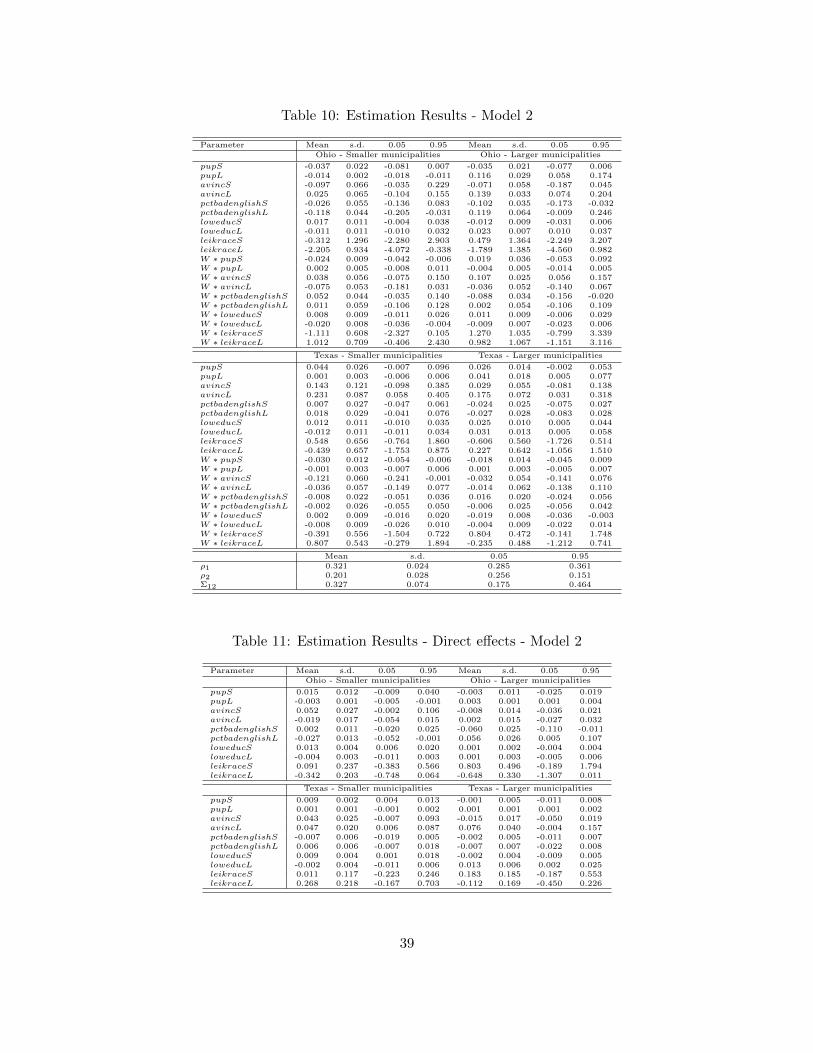
Table 10: Estimation Results - Model 2

Parameter Mean s.d. 0.05 0.95 Mean s.d. 0.05 0.95Ohio - Smaller municipalities Ohio - Larger municipalities

pupS -0.037 0.022 -0.081 0.007 -0.035 0.021 -0.077 0.006pupL -0.014 0.002 -0.018 -0.011 0.116 0.029 0.058 0.174avincS -0.097 0.066 -0.035 0.229 -0.071 0.058 -0.187 0.045avincL 0.025 0.065 -0.104 0.155 0.139 0.033 0.074 0.204pctbadenglishS -0.026 0.055 -0.136 0.083 -0.102 0.035 -0.173 -0.032pctbadenglishL -0.118 0.044 -0.205 -0.031 0.119 0.064 -0.009 0.246loweducS 0.017 0.011 -0.004 0.038 -0.012 0.009 -0.031 0.006loweducL -0.011 0.011 -0.010 0.032 0.023 0.007 0.010 0.037leikraceS -0.312 1.296 -2.280 2.903 0.479 1.364 -2.249 3.207leikraceL -2.205 0.934 -4.072 -0.338 -1.789 1.385 -4.560 0.982W ∗ pupS -0.024 0.009 -0.042 -0.006 0.019 0.036 -0.053 0.092W ∗ pupL 0.002 0.005 -0.008 0.011 -0.004 0.005 -0.014 0.005W ∗ avincS 0.038 0.056 -0.075 0.150 0.107 0.025 0.056 0.157W ∗ avincL -0.075 0.053 -0.181 0.031 -0.036 0.052 -0.140 0.067W ∗ pctbadenglishS 0.052 0.044 -0.035 0.140 -0.088 0.034 -0.156 -0.020W ∗ pctbadenglishL 0.011 0.059 -0.106 0.128 0.002 0.054 -0.106 0.109W ∗ loweducS 0.008 0.009 -0.011 0.026 0.011 0.009 -0.006 0.029W ∗ loweducL -0.020 0.008 -0.036 -0.004 -0.009 0.007 -0.023 0.006W ∗ leikraceS -1.111 0.608 -2.327 0.105 1.270 1.035 -0.799 3.339W ∗ leikraceL 1.012 0.709 -0.406 2.430 0.982 1.067 -1.151 3.116

Texas - Smaller municipalities Texas - Larger municipalities

pupS 0.044 0.026 -0.007 0.096 0.026 0.014 -0.002 0.053pupL 0.001 0.003 -0.006 0.006 0.041 0.018 0.005 0.077avincS 0.143 0.121 -0.098 0.385 0.029 0.055 -0.081 0.138avincL 0.231 0.087 0.058 0.405 0.175 0.072 0.031 0.318pctbadenglishS 0.007 0.027 -0.047 0.061 -0.024 0.025 -0.075 0.027pctbadenglishL 0.018 0.029 -0.041 0.076 -0.027 0.028 -0.083 0.028loweducS 0.012 0.011 -0.010 0.035 0.025 0.010 0.005 0.044loweducL -0.012 0.011 -0.011 0.034 0.031 0.013 0.005 0.058leikraceS 0.548 0.656 -0.764 1.860 -0.606 0.560 -1.726 0.514leikraceL -0.439 0.657 -1.753 0.875 0.227 0.642 -1.056 1.510W ∗ pupS -0.030 0.012 -0.054 -0.006 -0.018 0.014 -0.045 0.009W ∗ pupL -0.001 0.003 -0.007 0.006 0.001 0.003 -0.005 0.007W ∗ avincS -0.121 0.060 -0.241 -0.001 -0.032 0.054 -0.141 0.076W ∗ avincL -0.036 0.057 -0.149 0.077 -0.014 0.062 -0.138 0.110W ∗ pctbadenglishS -0.008 0.022 -0.051 0.036 0.016 0.020 -0.024 0.056W ∗ pctbadenglishL -0.002 0.026 -0.055 0.050 -0.006 0.025 -0.056 0.042W ∗ loweducS 0.002 0.009 -0.016 0.020 -0.019 0.008 -0.036 -0.003W ∗ loweducL -0.008 0.009 -0.026 0.010 -0.004 0.009 -0.022 0.014W ∗ leikraceS -0.391 0.556 -1.504 0.722 0.804 0.472 -0.141 1.748W ∗ leikraceL 0.807 0.543 -0.279 1.894 -0.235 0.488 -1.212 0.741

Mean s.d. 0.05 0.95ρ1 0.321 0.024 0.285 0.361ρ2 0.201 0.028 0.256 0.151Σ12 0.327 0.074 0.175 0.464

Table 11: Estimation Results - Direct effects - Model 2

Parameter Mean s.d. 0.05 0.95 Mean s.d. 0.05 0.95Ohio - Smaller municipalities Ohio - Larger municipalities

pupS 0.015 0.012 -0.009 0.040 -0.003 0.011 -0.025 0.019pupL -0.003 0.001 -0.005 -0.001 0.003 0.001 0.001 0.004avincS 0.052 0.027 -0.002 0.106 -0.008 0.014 -0.036 0.021avincL -0.019 0.017 -0.054 0.015 0.002 0.015 -0.027 0.032pctbadenglishS 0.002 0.011 -0.020 0.025 -0.060 0.025 -0.110 -0.011pctbadenglishL -0.027 0.013 -0.052 -0.001 0.056 0.026 0.005 0.107loweducS 0.013 0.004 0.006 0.020 0.001 0.002 -0.004 0.004loweducL -0.004 0.003 -0.011 0.003 0.001 0.003 -0.005 0.006leikraceS 0.091 0.237 -0.383 0.566 0.803 0.496 -0.189 1.794leikraceL -0.342 0.203 -0.748 0.064 -0.648 0.330 -1.307 0.011

Texas - Smaller municipalities Texas - Larger municipalities

pupS 0.009 0.002 0.004 0.013 -0.001 0.005 -0.011 0.008pupL 0.001 0.001 -0.001 0.002 0.001 0.001 0.001 0.002avincS 0.043 0.025 -0.007 0.093 -0.015 0.017 -0.050 0.019avincL 0.047 0.020 0.006 0.087 0.076 0.040 -0.004 0.157pctbadenglishS -0.007 0.006 -0.019 0.005 -0.002 0.005 -0.011 0.007pctbadenglishL 0.006 0.006 -0.007 0.018 -0.007 0.007 -0.022 0.008loweducS 0.009 0.004 0.001 0.018 -0.002 0.004 -0.009 0.005loweducL -0.002 0.004 -0.011 0.006 0.013 0.006 0.002 0.025leikraceS 0.011 0.117 -0.223 0.246 0.183 0.185 -0.187 0.553leikraceL 0.268 0.218 -0.167 0.703 -0.112 0.169 -0.450 0.226

39

Table 12: Estimation Results - Indirect effects - Model 2

Parameter Mean s.d. 0.05 0.95 Mean s.d. 0.05 0.95Ohio - Smaller municipalities Ohio - Larger municipalities

pupS 0.014 0.012 -0.010 0.038 0.006 0.015 -0.024 0.035pupL 0.001 0.001 -0.001 0.004 0.002 0.001 0.001 0.004avincS 0.062 0.019 0.024 0.101 -0.008 0.016 -0.041 0.024avincL -0.016 0.017 -0.051 0.018 0.002 0.022 -0.041 0.045pctbadenglishS 0.006 0.013 -0.021 0.033 -0.055 0.016 -0.087 -0.022

pctbadenglishL -0.038 0.009 -0.056 -0.020 0.042 0.024 -0.006 0.091loweducS 0.007 0.005 -0.003 0.016 0.001 0.003 -0.006 0.006loweducL -0.003 0.003 -0.010 0.004 0.001 0.004 -0.006 0.009leikraceS 0.085 0.301 -0.518 0.688 0.767 0.454 -0.141 1.675leikraceL -0.644 0.220 -1.084 -0.204 -0.815 0.307 -1.430 -0.201

Texas - Smaller municipalities Texas - Larger municipalities

pupS 0.009 0.007 -0.004 0.022 0.003 0.005 -0.008 0.013pupL 0.001 0.001 -0.002 0.001 0.001 0.001 -0.001 0.002avincS 0.052 0.030 -0.008 0.111 0.003 0.014 -0.026 0.031avincL 0.075 0.030 0.015 0.135 0.061 0.028 0.006 0.117pctbadenglishS -0.002 0.007 -0.016 0.011 -0.001 0.007 -0.014 0.013pctbadenglishL 0.010 0.009 -0.008 0.027 -0.010 0.010 -0.029 0.009loweducS 0.006 0.003 0.001 0.013 0.003 0.003 -0.004 0.010loweducL 0.002 0.004 -0.006 0.008 0.012 0.005 0.002 0.021leikraceS 0.070 0.168 -0.266 0.405 0.052 0.197 -0.341 0.445leikraceL 0.163 0.174 -0.184 0.511 0.024 0.173 -0.322 0.369

Table 13: Estimation Results - Total effects - Model 2

Parameter Mean s.d. 0.05 0.95 Mean s.d. 0.05 0.95Ohio - Smaller municipalities Ohio - Larger municipalities

pupS 0.029 0.024 -0.020 0.077 0.003 0.026 -0.048 0.054pupL -0.002 0.002 -0.006 0.002 0.004 0.002 0.001 0.008avincS 0.115 0.046 0.022 0.207 -0.016 0.030 -0.077 0.044avincL -0.036 0.034 -0.105 0.033 0.004 0.036 -0.068 0.077pctbadenglishS 0.009 0.025 -0.041 0.058 -0.115 0.041 -0.197 -0.033pctbadenglishL -0.065 0.022 -0.109 -0.021 0.098 0.050 -0.001 0.197loweducS 0.019 0.008 0.002 0.036 0.001 0.005 -0.011 0.010loweducL -0.007 0.007 -0.021 0.006 0.001 0.007 -0.011 0.014leikraceS 0.176 0.539 -0.901 1.254 1.570 0.950 -0.330 3.469leikraceL -0.986 0.423 -1.832 -0.140 -1.463 0.637 -2.736 -0.190

Texas - Smaller municipalities Texas - Larger municipalities

pupS 0.018 0.009 0.001 0.035 0.005 0.008 -0.011 0.022pupL 0.001 0.001 -0.003 0.003 0.001 0.002 -0.002 0.004avincS 0.094 0.055 -0.016 0.204 -0.002 0.025 -0.051 0.047avincL 0.121 0.050 0.021 0.222 0.133 0.060 0.013 0.253pctbadenglishS -0.010 0.013 -0.035 0.016 -0.003 0.009 -0.022 0.015pctbadenglishL 0.015 0.015 -0.015 0.045 -0.015 0.016 -0.047 0.016loweducS 0.016 0.007 0.001 0.030 0.003 0.004 -0.005 0.012loweducL -0.001 0.008 -0.016 0.014 0.024 0.009 0.005 0.042leikraceS 0.081 0.285 -0.489 0.651 0.141 0.272 -0.402 0.684leikraceL 0.432 0.391 -0.351 1.214 -0.052 0.313 -0.678 0.574

Table 14: Estimation Results - Correlated Random Effects - Model 2

Parameter Mean s.d. 0.05 0.95 Mean s.d. 0.05 0.95Smaller municipalities Larger municipalities

Cleveland 0.652 0.534 -0.416 1.720 -0.677 0.480 -1.637 0.283Cincinnati 0.485 0.563 -0.641 1.611 0.449 0.736 -1.022 1.920Colombus -1.390 0.610 -2.611 -0.170 0.467 0.989 -1.511 2.445Dayton -1.312 0.573 -2.458 -0.166 -0.244 0.722 -1.688 1.200Toledo -1.460 0.649 -2.758 -0.161 0.164 0.705 -1.246 1.574San Antonio -0.727 0.907 -2.541 1.086 0.293 0.696 -1.098 1.684Houston -1.894 0.766 -3.427 -0.361 -0.608 0.448 -1.504 0.287Dallas -1.870 0.613 -3.097 -0.644 -0.053 0.648 -1.350 1.243

40