public sector pay and corruption: measuring bribery from micro data
TRANSCRIPT

m/locate/econbase
Journal of Public Economics 91 (2007) 963–991www.elsevier.co
Public sector pay and corruption: Measuring briberyfrom micro data
Yuriy Gorodnichenko a, Klara Sabirianova Peter b,c,⁎
a University of Michigan, United Statesb Georgia State University, United States
c IZA Bonn, Germany
Received 16 February 2006; received in revised form 1 December 2006; accepted 6 December 2006Available online 16 January 2007
Abstract
This study provides the first systematic measure of bribery using micro-level data on reported earnings,household spending and asset holdings. We use the compensating differential framework and the estimatedsectoral gap in reported earnings and expenditures to identify the size of unobserved (unofficial)compensation (i.e., bribes) of public sector employees. In the case of Ukraine, we find that public sectoremployees receive 24–32% less wages than their private sector counterparts. The gap is particularly large atthe top of the wage distribution. At the same time, workers in both sectors have essentially identical level ofconsumer expenditures and asset holdings that unambiguously indicate the presence of non-reportedcompensation in the public sector. Using the conditions of labor market equilibrium, we develop anaggregate measure of bribery and find that the lower bound estimate of the extent of bribery in Ukraine isbetween 460 million and 580 million U.S. dollars (0.9–1.2% of Ukraine's GDP in 2003).© 2006 Elsevier B.V. All rights reserved.
JEL classification: D73; H1; J3; J4; O1; P2Keywords: Corruption; Bribery; Public sector; Wage; Wage differentials; Consumption; Ukraine
1. Introduction
Corruption undermines the strength of public institutions and hampers economic growth anddevelopment (Shleifer and Vishny, 1993; Mauro, 1995; Bardhan, 1997; Meon and Sekkat, 2005).The cost of corruption is particularly high in developing and transition countries where bribery is
⁎ Corresponding author. Georgia State University, United States. Tel.: +1 404 651 3986; fax: +1 404 651 4985.E-mail addresses: [email protected] (Y. Gorodnichenko), [email protected] (K. Sabirianova Peter).
0047-2727/$ - see front matter © 2006 Elsevier B.V. All rights reserved.doi:10.1016/j.jpubeco.2006.12.003

964 Y. Gorodnichenko, K. Sabirianova Peter / Journal of Public Economics 91 (2007) 963–991
endemic (EBRD, 2005; Transparency International, 2005). The question faced by the public andpolicy-makers is not whether corruption exists but its extent. Yet available estimates of bribery areimprecise, sporadic and apply to highly specific cases. Popular perception-based indices areordinal and subjective and while informative they do not provide a reliable quantitative estimateof bribery.
In this paper we develop a novel framework to estimate the extent of bribery in the publicsector using micro-level data on observable labor market outcomes, household spending, andasset holdings. Specifically, we estimate the residual wage differentials between the public andprivate sectors, compare these differentials with the sectoral differences in household expen-ditures and asset holdings, and then use the conditions of labor market equilibrium to compute amonetary value of unobserved non-taxable compensation (i.e., bribery) at the aggregate level.
We motivate our analysis by observing conflicting evidence from developed countries andseveral transition economies with respect to the private–public wage differentials. In a review ofpublic sector pay in several developed countries, Gregory and Borland (1999) conclude thatpublic sector employees generally receive higher average earnings than private sector employees.However, a few recent studies from transition countries find the opposite result, with public sectoremployees receiving much lower wages than their private sector counterparts (Adamchik andBedi (2000) in Poland, Brainerd (2002) in Russia, and Lokshin and Jovanovic (2003) inYugoslavia).
Using recently collected data from the Ukrainian Longitudinal Monitoring Survey, we alsofind that public sector employees in Ukraine are significantly underpaid compared to workers inthe other sectors. The wage gap between private and public firms is surprisingly large (24 to 32%conditional on worker characteristics) and remarkably stable over recent years (1997–2003). Weexamine the wage gap at different points of the conditional wage distribution and establish thataverage results understate the gap at the top and overstate it at the bottom of the distribution. Weshow that the wage gap is largest (can exceed 60%) among the most productive and highly paidworkers. At the same time, public and private sectors exhibit very similar rates of voluntaryseparations, labor mobility across sectors is non-trivial, the flows in and out of the public sectorare approximately the same, and the size of the public sector remains virtually unchanged over the7 years of our data. This brings about an important question of why public sector employees onaverage and the most productive workers in particular continue working in the public sectordespite their low rate of official pay.
We argue that bribery is the most likely explanation for the observed wage differences. Inparticular, we show that the wage gap remains large after correcting for endogeneity, controllingfor unobservable characteristics and accounting for differences in hours of work, job security,fringe benefits, bonuses, job satisfaction, and secondary employment. More importantly, we findthat the levels of consumer expenditures and asset holdings are essentially identical for workers inthe public and private sectors. This finding indicates unequivocally the presence of additionalnon-reported monetary compensation that allows employees in the public and private sectors toenjoy similar levels of consumption. We refer to this unobserved compensation in the publicsector as a bribe. We find that the gap between consumption and reported income is the largest forsubsectors of public administration and health care and for occupations of public sector managersand medical workers — groups that are commonly perceived as bribe takers and have also thegreatest opportunities to extract bribes.
The bribery explanation of the wage gap is consistent with a study of 31 developing countriesthat finds a robust negative relationship between aggregate corruption indices and relative civil-service pay at the country level (van Rijckeghem and Weder, 2001). This explanation is also

965Y. Gorodnichenko, K. Sabirianova Peter / Journal of Public Economics 91 (2007) 963–991
consistent with numerous media reports and surveys that portray widespread bribery in theUkrainian public sector. For example, according to the 2002 national survey of corruption inUkraine, 78% of the respondents believe that all or almost all government officials accept bribes,44% indicate that they paid bribes or made gifts in one form or another at least once during the lastyear (Woronowycz, 2003).1
The fact that bribery exists in Ukraine on a large scale is common knowledge and it has beenvery well documented in the literature and by the mass media. It is not something that we wouldlike to prove or disprove in this study. What we argue here is that when bribery is widespread andexists for many years, it should appear through sectoral differences in equilibrium wages andemployment flows, and we can use these differences to infer the size of bribery in the economy.
We estimate the extent of bribery at the national level by using the method of equalizingsectoral differences. There are three underlying assumptions of our method: (1) there is no briberyin the private sector, (2) there are no queues in the public sector, and (3) there is no risk of beingdetected taking bribes in the public sector. If any of these assumptions does not hold, weunderestimate the magnitude of bribery. Using our best estimates of the residual private–publicwage gap, we find that bribery accounts for at least 20% of the total wage compensation in thepublic sector in Ukraine, which is equivalent to 460–580 million U.S. dollars or 0.9–1.2% ofUkraine's GDP in 2003. Our alternative estimates suggest that the amount of bribery could be ashigh as 750 million U.S. dollars in 2003.
The paper is organized as follows. In Section 2 we introduce our data and descriptive statistics.In Section 3 we present the estimates of the private–public wage gap on average and at differentpoints in the wage distribution and check their robustness. In Section 4 we explore the factors thatmight explain the trends established in Section 3. We present the methodology and the estimatesof bribery in Ukraine in Section 5 and conclude in Section 6.
2. Data and sample
The data for this study are drawn from the Ukrainian Longitudinal Monitoring Survey(ULMS) which is based on a stratified, random, and nationally representative sample of 4096households. 8641 individuals of age 15–72 participated in the Ukrainian survey in 2003. Theresponse rate was 66% for households and 87% for individuals within the households. AlthoughULMS started only in 2003, it collected employment histories for 1986, 1991, and continuouslyfrom 1997 to 2003. In this paper we do not use the 1986 data because no respondent reports aprivate job for this year.
The ULMS contains rich information on household and individual characteristics such ashousehold expenditures and asset holdings, individual earnings, hours of work, education,demographics, job tenure, quits and layoffs, parents' occupation and education, and charac-teristics of the primary employer such as sector, location, size, and fringe benefits. The definitionsof all variables used in the empirical analysis are provided in Appendix Table A1.
The key variable in our analysis is the log of monthly contractual (accrued) wage after taxes atthe primary job. We refer readers to Gorodnichenko and Sabirianova (2005) for a discussion ofthe advantages and shortcomings of this measure and also for the effect of a recall bias on the
1 According to the same survey, 73% of the respondents indicated they had offered money to medical workers, 25%paid traffic police, 24% paid teachers and professors, 23% claimed they had illegally compensated governmentcommunal service workers (Woronowycz, 2003).
966 Y. Gorodnichenko, K. Sabirianova Peter / Journal of Public Economics 91 (2007) 963–991
wage measure in the ULMS. Ideally, we would like to use an hourly wage rate to control forsectoral differences in hours of work. However, we can create such a variable only for 2003 bydividing monthly wage by monthly hours of work at the primary job (calculated as averageweekly hours times 4.2). In all other years, the differences in hours are partially controlled byincluding a dummy variable for a full-time job.
To reduce the potential effect of mortality-related sample attrition in a retrospective survey, thesample is restricted to the prime age group 15–59. Following the literature (e.g., Borjas, 2002),we exclude the self-employed from the analysis of the private–public wage gap. We also leave outworker collectives (cooperatives and agricultural farms) because their wage determinationprocess is different from other private firms. These criteria produce the sample of wage earnersthat ranges from 2320 in 1998 to 2893 people in 1991.
We distinguish between the private sector and the two segments of the state sector —budgetary organizations and state-owned enterprises (SOEs) and define the public sector ascomprised of budgetary organizations. These are non-profit organizations that are financed byand fully accountable to the government, highly regulated, forced to pay according to thewage grid, and significantly influenced by the political environment. They typically providedirect services to the population, and hence employees of these organizations may receiveunofficial additional payments from customers for their services. The major categories ofbudgetary organizations are public administration, schools, and health care institutions.2 Incontrast, SOEs are mostly profit-driven institutions that are self-financed through theirown activities and managed by appointed directors who are given significant freedom indecision making. They often operate in concentrated or heavily regulated industries such asnatural resources, transportation, communications, the military industrial complex, andutilities. Wage payment according to the wage grid is recommended, but not strictly enforcedin SOEs. Despite these differences, SOEs and public organizations are very similar in manycharacteristics, including hours of work, fringe benefits, labor force composition, organi-zational norms, morale, etc. Therefore, working in SOEs might be a better counterfactualalternative for a public sector employee than working in the private sector (see Section 5 forfurther discussion).
The share of SOE employment in our sample continuously declined from 79.6% in 1991 to36.8% in 2003. In contrast, the private sector share increased from 1.3% in 1991 to 41.4% in2003. The growth of the private sector continued throughout the whole transition period — itssize increased by almost 64% from 1997 to 2002, which can be explained by large-scaleprivatization of state enterprises and by the entry of new private firms. In the meantime, theshare of public sector employment remained relatively unchanged over the last 12 years andstayed at 19–22%.
The summary statistics of the key variables are reported in Appendix Table A2. The share ofpublic sector employment is much larger for females than for males (31.3% vs. 10.6% in 2003).On average, the public sector employees (both males and females) are more educated thanemployees in state-owned and private firms. The public sector and SOEs display strongsimilarities in terms of average work experience, tenure, and hours of work. If in the privatesector the gender differences in all characteristics, except for education, are not statistically
2 Several studies of the private–public wage gap use similar definitions of the public sector. For example, Mueller(1998, 2000) includes in the public sector only those involved in public administration, health and education workers, anddoes not include government workers more closely related to other industries in Canada.

967Y. Gorodnichenko, K. Sabirianova Peter / Journal of Public Economics 91 (2007) 963–991
significant, in both state sectors females predictably stay longer at the same enterprise and workfewer hours.
3. Private–public wage gap
In this section, we document the evolution of the private–public wage gap in Ukraine andpresent various estimates of the gap, with a special emphasis on treating the endogeneity bias dueto omitted variables and self-selection.
Table 1 presents the summary statistics for the unconditional private–public wage gap inUkraine for all workers, and separately by gender. The gap is measured as a mean differencein log of monthly wage between the sectors. Evidently, SOEs and private firms pay anoticeable wage premium relative to public organizations for both males and females. Theaverage gap in 2003 was about 0.3 log points (33–36%). This finding is consistent with thepositive private sector wage premium (as compared to the entire state sector) found inseveral other transition countries (e.g., Brainerd (2002) in Russia and Lokshin and Jovanovic(2003) in Yugoslavia), but it contrasts with the negative gap observed in developedcountries.3
After controlling for the observable characteristics of workers, the conditional private–publicwage gap often reduces in absolute terms but remains negative and significant for females andsometimes takes on zero or a small positive value for males (Mueller, 1998; Poterba and Rueben,1994). Following the literature, we estimate the conditional gap from the wage equation for eachyear and gender:
lnwit ¼ Sitbþ Xitgþ eit; ð1Þ
where wit is after-tax monthly contractual wage, Sit is a set of indicators for working in SOEs orthe private sector; Xit is a vector of individual characteristics such as years of schooling, a genderdummy, experience, experience squared, tenure, tenure squared, a dummy for full-time job, sevencategories of firm size, and five categories of location; and εit is the error term.4 Table 1 shows theprivate–public wage gap ( β ) from Eq. (1) estimated for each year separately. The estimatedconditional wage gap remains large in economic and statistical levels and does not show any signof a decline from 1997 to 2003.5
3 For example, the mean difference in log of hourly wage between the private and public sectors is estimated to be−0.086 for males and −0.236 for females in UK in 1986 (Bender, 2003); −0.114 for both genders in Netherlands in 1986(van Ophem, 1993); −0.225 for males and −0.336 for females in Canada in 1990 (Prescott and Wandschneider, 1999);−0.009 for males and −0.165 for females in Germany in 1984–1996 (Jurges, 2002); and −0.060 for males and −0.200for females in Germany in 2000 (Melly, 2005), among many other studies.4 The choice of individual covariates is quite standard. Industry dummies are not included because they are perfectly
nested within the sectors. We are aware of a current debate whether it is appropriate to include the firm size variable(Gregory and Borland, 1999). We include the firm size in order to control partially for the unobservable differences innon-labor compensation and job security. Without this variable, the SOE–public gap increases by 0.03 log points whilethe private–public gap remains unaffected. The complete earnings functions estimates for the same data are reported inGorodnichenko and Sabirianova (2005).5 The colossal private sector wage premium in 1991 (0.482 log points or 62%) might seem somewhat inconsistent with
the rest of time-series. We note that the private sector virtually did not exist at that time (1.3% of non-farm employment)and the premium may simply reflect a first mover advantage for very few risk takers. For that reason we exclude the 1991data from the subsequent panel analysis and focus on the more mature transition period.
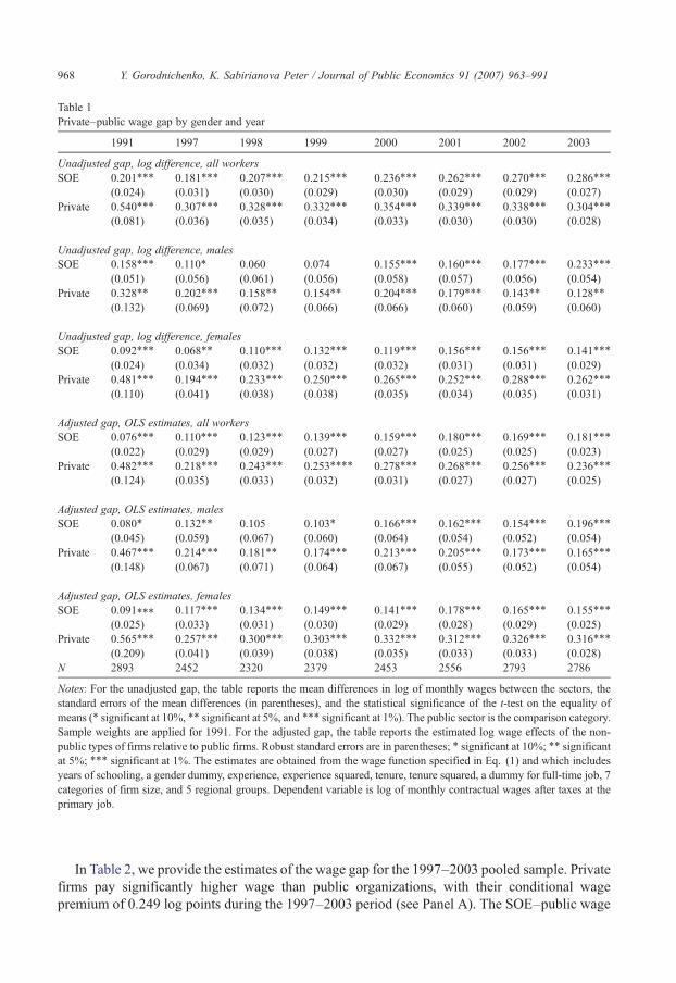
Table 1Private–public wage gap by gender and year
1991 1997 1998 1999 2000 2001 2002 2003
Unadjusted gap, log difference, all workersSOE 0.201⁎⁎⁎ 0.181⁎⁎⁎ 0.207⁎⁎⁎ 0.215⁎⁎⁎ 0.236⁎⁎⁎ 0.262⁎⁎⁎ 0.270⁎⁎⁎ 0.286⁎⁎⁎
(0.024) (0.031) (0.030) (0.029) (0.030) (0.029) (0.029) (0.027)Private 0.540⁎⁎⁎ 0.307⁎⁎⁎ 0.328⁎⁎⁎ 0.332⁎⁎⁎ 0.354⁎⁎⁎ 0.339⁎⁎⁎ 0.338⁎⁎⁎ 0.304⁎⁎⁎
(0.081) (0.036) (0.035) (0.034) (0.033) (0.030) (0.030) (0.028)
Unadjusted gap, log difference, malesSOE 0.158⁎⁎⁎ 0.110⁎ 0.060 0.074 0.155⁎⁎⁎ 0.160⁎⁎⁎ 0.177⁎⁎⁎ 0.233⁎⁎⁎
(0.051) (0.056) (0.061) (0.056) (0.058) (0.057) (0.056) (0.054)Private 0.328⁎⁎ 0.202⁎⁎⁎ 0.158⁎⁎ 0.154⁎⁎ 0.204⁎⁎⁎ 0.179⁎⁎⁎ 0.143⁎⁎ 0.128⁎⁎
(0.132) (0.069) (0.072) (0.066) (0.066) (0.060) (0.059) (0.060)
Unadjusted gap, log difference, femalesSOE 0.092⁎⁎⁎ 0.068⁎⁎ 0.110⁎⁎⁎ 0.132⁎⁎⁎ 0.119⁎⁎⁎ 0.156⁎⁎⁎ 0.156⁎⁎⁎ 0.141⁎⁎⁎
(0.024) (0.034) (0.032) (0.032) (0.032) (0.031) (0.031) (0.029)Private 0.481⁎⁎⁎ 0.194⁎⁎⁎ 0.233⁎⁎⁎ 0.250⁎⁎⁎ 0.265⁎⁎⁎ 0.252⁎⁎⁎ 0.288⁎⁎⁎ 0.262⁎⁎⁎
(0.110) (0.041) (0.038) (0.038) (0.035) (0.034) (0.035) (0.031)
Adjusted gap, OLS estimates, all workersSOE 0.076⁎⁎⁎ 0.110⁎⁎⁎ 0.123⁎⁎⁎ 0.139⁎⁎⁎ 0.159⁎⁎⁎ 0.180⁎⁎⁎ 0.169⁎⁎⁎ 0.181⁎⁎⁎
(0.022) (0.029) (0.029) (0.027) (0.027) (0.025) (0.025) (0.023)Private 0.482⁎⁎⁎ 0.218⁎⁎⁎ 0.243⁎⁎⁎ 0.253⁎⁎⁎⁎ 0.278⁎⁎⁎ 0.268⁎⁎⁎ 0.256⁎⁎⁎ 0.236⁎⁎⁎
(0.124) (0.035) (0.033) (0.032) (0.031) (0.027) (0.027) (0.025)
Adjusted gap, OLS estimates, malesSOE 0.080⁎ 0.132⁎⁎ 0.105 0.103⁎ 0.166⁎⁎⁎ 0.162⁎⁎⁎ 0.154⁎⁎⁎ 0.196⁎⁎⁎
(0.045) (0.059) (0.067) (0.060) (0.064) (0.054) (0.052) (0.054)Private 0.467⁎⁎⁎ 0.214⁎⁎⁎ 0.181⁎⁎ 0.174⁎⁎⁎ 0.213⁎⁎⁎ 0.205⁎⁎⁎ 0.173⁎⁎⁎ 0.165⁎⁎⁎
(0.148) (0.067) (0.071) (0.064) (0.067) (0.055) (0.052) (0.054)
Adjusted gap, OLS estimates, femalesSOE 0.091⁎⁎⁎ 0.117⁎⁎⁎ 0.134⁎⁎⁎ 0.149⁎⁎⁎ 0.141⁎⁎⁎ 0.178⁎⁎⁎ 0.165⁎⁎⁎ 0.155⁎⁎⁎
(0.025) (0.033) (0.031) (0.030) (0.029) (0.028) (0.029) (0.025)Private 0.565⁎⁎⁎ 0.257⁎⁎⁎ 0.300⁎⁎⁎ 0.303⁎⁎⁎ 0.332⁎⁎⁎ 0.312⁎⁎⁎ 0.326⁎⁎⁎ 0.316⁎⁎⁎
(0.209) (0.041) (0.039) (0.038) (0.035) (0.033) (0.033) (0.028)N 2893 2452 2320 2379 2453 2556 2793 2786
Notes: For the unadjusted gap, the table reports the mean differences in log of monthly wages between the sectors, thestandard errors of the mean differences (in parentheses), and the statistical significance of the t-test on the equality ofmeans (⁎ significant at 10%, ⁎⁎ significant at 5%, and ⁎⁎⁎ significant at 1%). The public sector is the comparison category.Sample weights are applied for 1991. For the adjusted gap, the table reports the estimated log wage effects of the non-public types of firms relative to public firms. Robust standard errors are in parentheses; ⁎ significant at 10%; ⁎⁎ significantat 5%; ⁎⁎⁎ significant at 1%. The estimates are obtained from the wage function specified in Eq. (1) and which includesyears of schooling, a gender dummy, experience, experience squared, tenure, tenure squared, a dummy for full-time job, 7categories of firm size, and 5 regional groups. Dependent variable is log of monthly contractual wages after taxes at theprimary job.
968 Y. Gorodnichenko, K. Sabirianova Peter / Journal of Public Economics 91 (2007) 963–991
In Table 2, we provide the estimates of the wage gap for the 1997–2003 pooled sample. Privatefirms pay significantly higher wage than public organizations, with their conditional wagepremium of 0.249 log points during the 1997–2003 period (see Panel A). The SOE–public wage
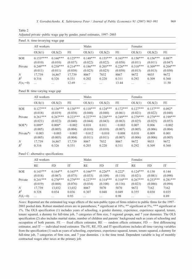
Table 2Adjusted private–public wage gap by gender, panel estimates, 1997–2003
Panel A: time-invarying wage gap
All workers Males Females
OLS(1) OLS(2) FE OLS(1) OLS(2) FE OLS(1) OLS(2) FE
SOE 0.153⁎⁎⁎⁎ 0.160⁎⁎⁎ 0.125⁎⁎⁎ 0.148⁎⁎⁎ 0.155⁎⁎⁎ 0.165⁎⁎⁎ 0.150⁎⁎⁎ 0.156⁎⁎⁎ 0.087⁎
(0.010) (0.010) (0.037) (0.022) (0.022) (0.058) (0.011) (0.011) (0.047)Private 0.249⁎⁎⁎ 0.258⁎⁎⁎ 0.214⁎⁎⁎ 0.186⁎⁎⁎ 0.205⁎⁎⁎ 0.226⁎⁎⁎ 0.310⁎⁎⁎ 0.309⁎⁎⁎ 0.204⁎⁎⁎
(0.011) (0.011) (0.038) (0.023) (0.023) (0.058) (0.013) (0.013) (0.050)N 17,739 16,867 17,739 8067 7832 8067 9672 9035 9672R2 0.316 0.326 0.331 0.202 0.220 0.311 0.292 0.309 0.360F(αi=0) … … 12.69 … … 13.44 … … 11.50
Panel B: time-varying wage gap
All workers Males Females
OLS(1) OLS(2) FE OLS(1) OLS(2) FE OLS(1) OLS(2) FE
SOE 0.127⁎⁎⁎ 0.136⁎⁎⁎ 0.130⁎⁎⁎ 0.118⁎⁎⁎ 0.124⁎⁎⁎ 0.172⁎⁎⁎ 0.127⁎⁎⁎ 0.137⁎⁎⁎ 0.092⁎
(0.018) (0.019) (0.038) (0.040) (0.040) (0.061) (0.021) (0.022) (0.048)Private 0.261⁎⁎⁎ 0.267⁎⁎⁎ 0.223⁎⁎⁎ 0.227⁎⁎⁎ 0.238⁎⁎⁎ 0.249⁎⁎⁎ 0.279⁎⁎⁎ 0.279⁎⁎⁎ 0.199⁎⁎⁎
(0.021) (0.022) (0.040) (0.044) (0.043) (0.063) (0.025) (0.025) (0.053)SOE⁎t 0.009⁎ 0.008⁎ −0.002 0.010 0.011 −0.003 0.007 0.006 −0.002
(0.005) (0.005) (0.004) (0.010) (0.010) (0.007) (0.005) (0.006) (0.004)Private⁎t −0.003 −0.003 −0.003 −0.012 −0.010 −0.008 0.010 0.009 0.001
(0.005) (0.005) (0.004) (0.011) (0.011) (0.007) (0.006) (0.006) (0.005)N 17,739 16,867 17,739 8067 7832 8067 9672 9035 9672R2 0.316 0.326 0.331 0.203 0.220 0.311 0.292 0.309 0.360
Panel C: alternative specifications
All workers Males Females
RE FD IT RE FD IT RE FD IT
SOE 0.143⁎⁎⁎ 0.164⁎⁎ 0.165⁎⁎ 0.166⁎⁎⁎ 0.226⁎⁎ 0.222⁎ 0.124⁎⁎⁎ 0.130 0.144(0.018) (0.067) (0.075) (0.033) (0.109) (0.118) (0.021) (0.081) (0.090)
Private 0.241⁎⁎⁎ 0.270⁎⁎⁎ 0.279⁎⁎⁎ 0.227⁎⁎⁎ 0.314⁎⁎⁎ 0.310⁎⁎⁎ 0.267⁎⁎⁎ 0.253⁎⁎⁎ 0.281⁎⁎⁎
(0.019) (0.068) (0.076) (0.034) (0.108) (0.116) (0.023) (0.086) (0.094)N 17,739 13,032 13,032 8067 5870 5870 9672 7162 7162R2 0.328 0.034 0.036 0.307 0.048 0.049 0.355 0.030 0.035F(δi=0) … … 0.93 … … 0.98 … … 0.89
Notes: Reported are the estimated log wage effects of the non-public types of firms relative to public firms for the 1997–2003 pooled data. Robust standard errors are in parentheses; ⁎ significant at 10%; ⁎⁎ significant at 5%; ⁎⁎⁎ significant at1%. The OLS specification (1) includes years of schooling, a gender dummy, experience, experience squared, tenure,tenure squared, a dummy for full-time job, 7 categories of firm size, 5 regional groups, and 7 year dummies. The OLSspecification (2) also includes marital status, number of children and parents' background such as years of schooling andoccupation of both parents. FE — fixed effects estimator, RE — random effects estimator, FD — first differencingestimator, and IT— individual trend estimator. The FE, RE, FD, and IT specifications includes all time-varying variablesfrom the specification (1) such as years of schooling, experience, experience squared, tenure, tenure squared, a dummy forfull-time job, 7 categories of firm size, and 7 year dummies. t is the time trend. Dependent variable is log of monthlycontractual wages after taxes at the primary job.
969Y. Gorodnichenko, K. Sabirianova Peter / Journal of Public Economics 91 (2007) 963–991

970 Y. Gorodnichenko, K. Sabirianova Peter / Journal of Public Economics 91 (2007) 963–991
gap is also large and highly significant (0.153 log points). Estimates in Panel B confirm thatsectoral wage differences are not diminishing over time. It is interesting that the conditionalprivate–public wage gap is noticeably higher for females than for males (0.310 vs. 0.186 logpoints), whereas we know from previous research in developed countries that females usuallyenjoy a bigger wage premium in the public sector, with or without conditioning on workercharacteristics (Borjas, 2002; Prescott and Wandschneider, 1999).
Our OLS estimates may be biased due to omitted variables and endogenous self-selection tothe public sector. Among the “usual suspects” of omitted factors are individual abilities, pre-ferences, family or neighborhood influence, etc. The most obvious solution to this problem is toadd omitted variables or their proxies into a wage equation. Cross-sectional data could offer apartial treatment because of the limited number of available proxies such as test scores, parentalbackground, number of children, place of residence, etc. Fixed effect estimates are superior in thatthey control for all time-invariant omitted variables that might affect both wage and sectoralchoice, including unobserved abilities, sectoral preferences, accumulated family wealth, andparental influence.6
In Table 2, column OLS(2), we report the conditional private–public wage gap estimated fromthe wage equation that includes all covariates from OLS(1) plus marital status, number ofchildren, and several variables for family background — ten categories of occupations and yearsof schooling of both parents. In Table 2 we also show the fixed effect (FE) estimates of the gapfrom Eq. (2):7
lnwit ¼ Sitbþ Xitgþ ai þ uit; ð2Þ
where αi are individual fixed effects.Both OLS(2) and FE estimates indicate that the private–public wage gap is economically
large, statistically significant, and not diminishing over time. The gap estimated with controls forchildren and family background is not statistically different from its original OLS estimate at the5% level of significance. Furthermore, the estimated gap for males is hardly influenced by fixedeffects, while the gap for females falls in FE compared to its original OLS estimate (from 0.310 to0.204 log points). This suggests that endogenous sorting into the public sector might be moreimportant for females than for males.8
6 Alternatively, the endogeneity bias can be addressed by using instrumental variables or switching regression models.These methods, however, require an exclusion restriction that affects strongly the choice of the sector and that is notcorrelated with the wage equation error term. Having experimented with a number of commonly used exclusionrestrictions (such as marital status, number of children, parents' occupation, household income, employment in pre-reform period, etc.), we conclude that the wage gap estimates corrected for self-selection are extremely sensitive to thechoice of exclusion restrictions and thus not credible. These estimates are reported and discussed in the associatedworking paper (Gorodnichenko and Sabirianova Peter, 2006). Most of the potentially valid exclusion restrictions aretime-invariant (or hardly change over time) and, therefore, these alternatives are not superior to the fixed effectspecification.7 In Table 2, panel C, we also report the random effect (RE) and first-differencing (FD) estimates of the wage gap but
note that the RE estimate cannot be considered as unbiased by the virtue of our assumption that αi influence sectoralchoice, i.e., E(Sit, αi)≠0. Both RE and FD estimates of the gap are close to the OLS estimate.8 Stronger preferences of females for fewer hours of work and higher job security may partly explain why endogenous
sorting into the public sector is more important for females than for males.
971Y. Gorodnichenko, K. Sabirianova Peter / Journal of Public Economics 91 (2007) 963–991
The FE estimates could be criticized for treating only the time-invariant portion of theendogeneity bias while preferences for a particular sector may change over time. To capture thispossible time-varying endogeneity, we estimate an individual trend model that allows individualunobserved factors to have their own time trend:
lnwit ¼ Sitbþ Xitgþ ai þ dit þ uit: ð3Þ
We first eliminate the constant individual effect αi by first-differencing transformation of allvariables, and then we apply the fixed effects transformation to Eq. (4) in order to eliminate theindividual-specific trend δi:
9
Dlnwit ¼ DSitbþ DXitgþ di þ Duit: ð4Þ
We note that such a transformation, while treating endogeneity, can generate several problems.First, it might lead to the attenuation bias due to an increased noise-to-signal ratio, especiallywhen the number of people who switch sectors is small. This is less of a problem in our data sincethe number of people changing sectors is non-trivial. Among those employed in the public sectorin 1997, 63% continued working in this sector during next six years, while the remaining 37% leftthe sector either temporary or permanently. If we take only employees in our three sectors, about12% of them switched sectors directly (without a break for non-employment or self-employment)at least once during the 1997–2003 period. Second, applying FE to a first-differenced equationtends to magnify standard errors due to a smaller sample size, reduced variation in regressors, andincreased variation of the error term. Despite these problems, the individual trend estimate of theprivate–public wage gap is large in magnitude (0.279 log points) and statistically significant(Table 2, Panel C).
In summary, all panel data estimates of the gap appear to be very close to the baseline OLSestimates and indicate that public sector employees are significantly underpaid compared toemployees in SOEs and private firms, with an estimated conditional wage loss varying from0.214 to 0.279 log points relative to private sector wages and from 0.125 to 0.165 log pointsrelative to SOEs wages.
We also estimate a series of quantile regressions to examine the private–public wage gap atdifferent percentiles of conditional wage distribution:
QhðlnwitjSit;XitÞ ¼ Sitbh þ Xitgh; ð5Þ
whereQθ is the θth percentile of lnwit conditional on the covariates S and X specified in OLS(1).10
The estimated coefficients βθ give the conditional wage gap at the θth percentile. The distributionof these coefficients is depicted in Fig. 1 (see distributions for contractual monthly wages).
9 The FE estimator is more efficient than the second differencing estimator under the assumption that Δuit are seriallyuncorrelated.10 We use the set of covariates specified in OLS(1) because including additional covariates from OLS(2) reduces thesample size significantly and the OLS(1) specification makes our estimates more comparable to other studies given thatfamily background and children variables are not easily available in many surveys. As discussed in Section 3, theadditional covariates do not have a statistically significant effect on the estimated wage gap.
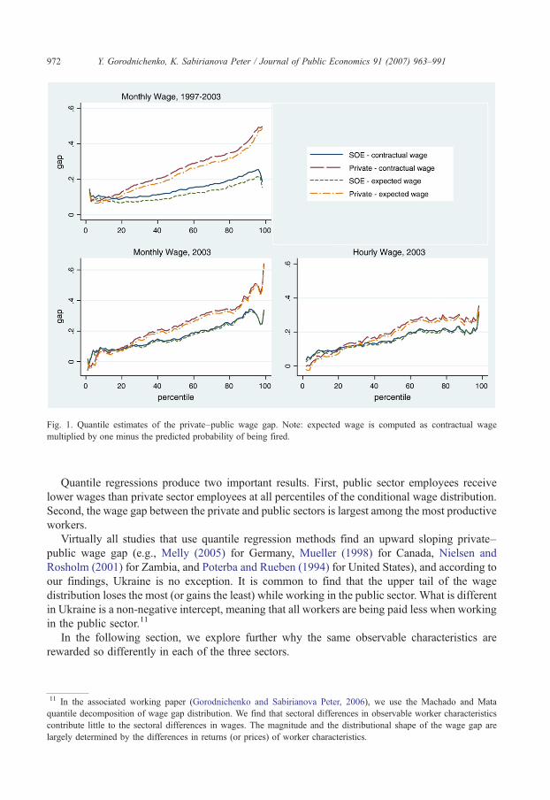
Fig. 1. Quantile estimates of the private–public wage gap. Note: expected wage is computed as contractual wagemultiplied by one minus the predicted probability of being fired.
972 Y. Gorodnichenko, K. Sabirianova Peter / Journal of Public Economics 91 (2007) 963–991
Quantile regressions produce two important results. First, public sector employees receivelower wages than private sector employees at all percentiles of the conditional wage distribution.Second, the wage gap between the private and public sectors is largest among the most productiveworkers.
Virtually all studies that use quantile regression methods find an upward sloping private–public wage gap (e.g., Melly (2005) for Germany, Mueller (1998) for Canada, Nielsen andRosholm (2001) for Zambia, and Poterba and Rueben (1994) for United States), and according toour findings, Ukraine is no exception. It is common to find that the upper tail of the wagedistribution loses the most (or gains the least) while working in the public sector. What is differentin Ukraine is a non-negative intercept, meaning that all workers are being paid less when workingin the public sector.11
In the following section, we explore further why the same observable characteristics arerewarded so differently in each of the three sectors.
11 In the associated working paper (Gorodnichenko and Sabirianova Peter, 2006), we use the Machado and Mataquantile decomposition of wage gap distribution. We find that sectoral differences in observable worker characteristicscontribute little to the sectoral differences in wages. The magnitude and the distributional shape of the wage gap arelargely determined by the differences in returns (or prices) of worker characteristics.

973Y. Gorodnichenko, K. Sabirianova Peter / Journal of Public Economics 91 (2007) 963–991
4. Determinants of the private–public wage gap
To this point of our analysis, we have established three important patterns in sectoral wagedifferentials in Ukraine: (i) the private–public wage gap is positive and economically significant;(ii) the gap is not diminishing over time; and (iii) the gap is largest among the most productiveworkers. This section investigates the factors that might explain these patterns.12 In particular, wefocus on wage control in an inflationary environment, differences in hours of work, non-laborcompensation, job security, job satisfaction, multiple job holding, and bribery.
4.1. Government wage control
Wages in the public sector in Ukraine are paid according to a government-regulated wage grid.In an inflationary economy such as Ukraine, delayed revisions of the wage grid might result inlower wages in the public sector. It could have been an important issue during the early 1990swhen Ukraine experienced a hyperinflation of three to four digits, reaching the 4735% level in1993. After 1996, inflation was relatively mild and fluctuated from 28.2% in 2000 to 0.8% in2002. During the 1997–2003 period, the government implemented eight revisions of the wagegrid level in the public sector, yet the gap remained large. More importantly, the fact that publicemployees are constantly underpaid due to delayed and imperfect adjustments in the wage griddoes not explain why we do not observe higher quit rates in the public sector, as shown below.
4.2. Hours of work
As we see from the descriptive statistics in Table A2, a public sector employee, on average,works fewer hours per week than a private sector employee, with a 3-hour difference for malesand a 7-hour difference for females. It may not be sufficient to simply control for a full-time job aswe did it in our previous estimates. It is predictable that the estimated wage gap is likely to declineif we were to use hourly wages instead of monthly wages. For 2003, we can test how sensitive ourgap estimates to hourly wages are by using OLS and quantile regressions.
We report our results in Table 3 and Fig. 1. To reduce the influence of outliers and ameasurement error, we include only respondents who earn more than two thirds of a minimumhourly wage (≈0.734 UAH). Using hourly wage rate as a dependent variable in Eq. (1) reducesthe size of the SOE–public wage gap by only 0.036 log points while the private–public gap fallsfrom 0.287 to 0.193 log points. As a side note, Table 3 also shows that restricting our sample tofull-time employees does not make any difference for the reduction in the size of the gap. Themost interesting finding from the quantile regressions (depicted on Fig. 1) is that with an hourlycontractual wage rate on the left-hand side the private–SOE gap reduces significantly while theSOE–public gap remains the same at nearly all percentiles of conditional wage distribution. Animportant implication of this finding is that in the absence of hours of work variable the SOE–public gap can be used as an approximate measure of the private–public gap.
12 Previous studies focused on explanations of the opposite phenomenon, that is, why a public sector employee earns a rent(i.e., positive wage premium conditional onworker characteristics). Themost common answer is the specificity of the publicsector, namely, its different objective function (not profit maximization) and soft budget constraints, inelastic demand forpublic services, difficult monitoring of public sector services, and a higher rate of unionization and hence stronger bargainingposition to secure a higher wage (Mueller, 2000). If any of these factors are relevant for Ukraine, then the size of the private–public gap would be even bigger than the estimates reported in Section 3. However, we did not find statistically significantdifferences in wages associated with union membership in Ukraine (Gorodnichenko and Sabirianova Peter, 2006).
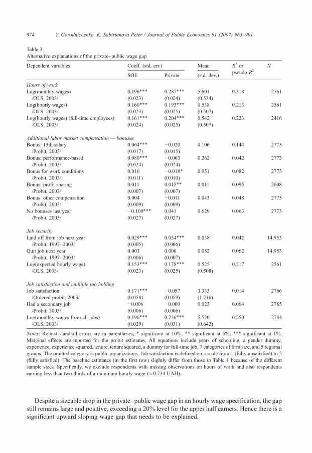
Table 3Alternative explanations of the private–public wage gap
Dependent variables: Coeff. (std. err.) Mean R2 orpseudo R2
N
SOE Private (std. dev.)
Hours of workLog(monthly wages) 0.196⁎⁎⁎ 0.287⁎⁎⁎ 5.601 0.318 2561
/OLS, 2003/ (0.023) (0.024) (0.534)Log(hourly wages) 0.160⁎⁎⁎ 0.193⁎⁎⁎ 0.538 0.213 2561
/OLS, 2003/ (0.023) (0.025) (0.507)Log(hourly wages) (full-time employees) 0.161⁎⁎⁎ 0.204⁎⁎⁎ 0.542 0.223 2416
/OLS, 2003/ (0.024) (0.025) (0.507)
Additional labor market compensation — bonusesBonus: 13th salary 0.064⁎⁎⁎ −0.020 0.106 0.144 2773
/Probit, 2003/ (0.017) (0.015)Bonus: performance-based 0.080⁎⁎⁎ −0.003 0.262 0.042 2773
/Probit, 2003/ (0.024) (0.024)Bonus for work conditions 0.016 −0.018⁎ 0.051 0.082 2773
/Probit, 2003/ (0.011) (0.010)Bonus: profit sharing 0.011 0.015⁎⁎ 0.011 0.095 2608
/Probit, 2003/ (0.007) (0.007)Bonus: other compensation 0.004 −0.011 0.043 0.048 2773
/Probit, 2003/ (0.009) (0.009)No bonuses last year −0.100⁎⁎⁎ 0.041 0.629 0.063 2773
/Probit, 2003/ (0.027) (0.027)
Job securityLaid off from job next year 0.029⁎⁎⁎ 0.034⁎⁎⁎ 0.038 0.042 14,953
/Probit, 1997–2003/ (0.005) (0.006)Quit job next year 0.003 0.006 0.082 0.062 14,953
/Probit, 1997–2003/ (0.006) (0.007)Log(expected hourly wage) 0.153⁎⁎⁎ 0.178⁎⁎⁎ 0.525 0.217 2561
/OLS, 2003/ (0.023) (0.025) (0.508)
Job satisfaction and multiple job holdingJob satisfaction 0.171⁎⁎⁎ −0.057 3.333 0.014 2766
/Ordered probit, 2003/ (0.058) (0.059) (1.216)Had a secondary job −0.006 −0.000 0.023 0.064 2785
/Probit, 2003/ (0.006) (0.006)Log(monthly wages from all jobs) 0.196⁎⁎⁎ 0.236⁎⁎⁎ 5.520 0.250 2784
/OLS, 2003/ (0.029) (0.031) (0.642)
Notes: Robust standard errors are in parentheses; ⁎ significant at 10%; ⁎⁎ significant at 5%; ⁎⁎⁎ significant at 1%.Marginal effects are reported for the probit estimates. All equations include years of schooling, a gender dummy,experience, experience squared, tenure, tenure squared, a dummy for full-time job, 7 categories of firm size, and 5 regionalgroups. The omitted category is public organizations. Job satisfaction is defined on a scale from 1 (fully unsatisfied) to 5(fully satisfied). The baseline estimates (in the first row) slightly differ from those in Table 1 because of the differentsample sizes. Specifically, we exclude respondents with missing observations on hours of work and also respondentsearning less than two thirds of a minimum hourly wage (≈0.734 UAH).
974 Y. Gorodnichenko, K. Sabirianova Peter / Journal of Public Economics 91 (2007) 963–991
Despite a sizeable drop in the private–public wage gap in an hourly wage specification, the gapstill remains large and positive, exceeding a 20% level for the upper half earners. Hence there is asignificant upward sloping wage gap that needs to be explained.

975Y. Gorodnichenko, K. Sabirianova Peter / Journal of Public Economics 91 (2007) 963–991
4.3. Fringe benefits and total labor compensation
More generous fringe benefits in the public sector may compensate lower wages. Compared toprivate firms, public organizations in Ukraine are more likely to provide their employees withadditional medical services, free child care, vacation travel, housing subsidies, and enterprise-paid training (Table 4). Thus, it is plausible to hypothesize that total labor compensation (wagesplus fringe benefits) could be equalized between the sectors.
However, several facts invalidate this hypothesis. First, there are almost no differences in fringebenefits provision between the public sectors and SOEs and in some instances more workersreceive benefits in SOEs than in public organizations (e.g., health coverage and transportationsubsidies). Consequently, fringe benefits cannot explain the observed wage differences betweenthe two state sectors. Second, the distribution of fringe benefits across the percentiles of con-ditional wage is practically flat in all sectors, as depicted in Fig. 2 for the selected benefits. The flatdistribution of fringe benefits does not support the upward sloping private–public gap. Even if weassume that fringe benefits account for the wage differences between SOEs and private firms, asignificant portion of the private–public gap, particularly for the most productive workers, remainsunexplained.
We also compare mean probabilities of receiving five types of bonuses across sectors usingmarginal effects from the probit model shown in Table 3. 37.1% of the sample report getting abonus last year, although the exact bonus amount is unknown. In most specifications, cross-sectoral differences in probabilities of getting bonuses are not statistically significant at the 5%level, with an exception of a higher incidence of receiving a 13th salary and performance-basedbonuses in SOEs, and a higher probability of profit sharing in the private sector. Based on thesefindings, adding bonus amounts to wages on the LHS is likely to increase the conditional private–public wage gap (or at least not to change it).
Alternative firm-level data sources also suggest that the sectoral differences in total laborcompensation might be bigger than pure wage differentials. Despite the lower percent of privatesector workers receiving fringe benefits, the value of social expenditures is higher in privateenterprises than in public organizations, perhaps reflecting the budgetary difficulties of financingsocial programs in budgetary organizations. In budgetary non-profit organizations, the averageshare of social benefits in total labor costs (weighted by firm employment) is 23% whereas thebenefit share in state-owned enterprises is 27% and private non-farm firms is 26%.13 Thus, ifworkers were able to assess the value of their fringe benefits and bonuses, then the estimatedsectoral gap in total labor compensation would have been larger.
4.4. Job security and risk aversion
Job security is another important factor that enters into a tradeoff with wage. Public sectoremployees may accept lower wages in exchange for higher job security. We can approximateindividual job security by the probability of layoffs and also by the degree of wage volatility.
13 Both mean differences in the share of benefits are statistically significant at the 1% level. Social benefits includeexpenditures on housing provision and housing subsidies of employees, cost of professional training, cost of workers'recreation and entertainment, health care payments, child care allowances and services, employer contribution togovernment social security schemes and private social funds, and other related expenditures. The firm-level datarepresent the whole population of the registered Ukrainian firms that have submitted their labor cost statistics to the StateStatistics Committee in 2002 (50,400 firms with total employment of 8.5 million workers).
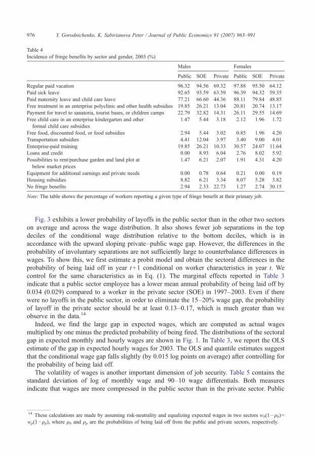
Table 4Incidence of fringe benefits by sector and gender, 2003 (%)
Males Females
Public SOE Private Public SOE Private
Regular paid vacation 96.32 94.56 69.32 97.88 95.50 64.12Paid sick leave 92.65 93.59 63.59 96.39 94.32 59.35Paid maternity leave and child care leave 77.21 66.60 44.36 88.11 79.84 48.85Free treatment in an enterprise polyclinic and other health subsidies 19.85 26.21 13.04 20.81 20.74 13.17Payment for travel to sanatoria, tourist bases, or children camps 22.79 32.82 14.31 26.11 29.55 14.69Free child care in an enterprise kindergarten and other
formal child care subsidies1.47 5.44 3.18 2.12 1.96 1.72
Free food, discounted food, or food subsidies 2.94 5.44 3.02 0.85 1.96 4.20Transportation subsidies 4.41 12.04 3.97 3.40 9.00 4.01Enterprise-paid training 19.85 26.21 10.33 30.57 24.07 11.64Loans and credit 0.00 8.93 6.04 2.76 8.02 5.92Possibilities to rent/purchase garden and land plot at
below market prices1.47 6.21 2.07 1.91 4.31 4.20
Equipment for additional earnings and private needs 0.00 0.78 0.64 0.21 0.00 0.19Housing subsidies 8.82 6.21 3.34 8.07 5.28 3.82No fringe benefits 2.94 2.33 22.73 1.27 2.74 30.15
Note: The table shows the percentage of workers reporting a given type of fringe benefit at their primary job.
976 Y. Gorodnichenko, K. Sabirianova Peter / Journal of Public Economics 91 (2007) 963–991
Fig. 3 exhibits a lower probability of layoffs in the public sector than in the other two sectorson average and across the wage distribution. It also shows fewer job separations in the topdeciles of the conditional wage distribution relative to the bottom deciles, which is inaccordance with the upward sloping private–public wage gap. However, the differences in theprobability of involuntary separations are not sufficiently large to counterbalance differences inwages. To show this, we first estimate a probit model and obtain the sectoral differences in theprobability of being laid off in year t+1 conditional on worker characteristics in year t. Wecontrol for the same characteristics as in Eq. (1). The marginal effects reported in Table 3indicate that a public sector employee has a lower mean annual probability of being laid off by0.034 (0.029) compared to a worker in the private sector (SOE) in 1997–2003. Even if therewere no layoffs in the public sector, in order to eliminate the 15–20% wage gap, the probabilityof layoff in the private sector should be at least 0.13–0.17, which is much greater than weobserve in the data.14
Indeed, we find the large gap in expected wages, which are computed as actual wagesmultiplied by one minus the predicted probability of being fired. The distributions of the sectoralgap in expected monthly and hourly wages are shown in Fig. 1. In Table 3, we report the OLSestimate of the gap in expected hourly wages for 2003. The OLS and quantile estimates suggestthat the conditional wage gap falls slightly (by 0.015 log points on average) after controlling forthe probability of being laid off.
The volatility of wages is another important dimension of job security. Table 5 contains thestandard deviation of log of monthly wage and 90–10 wage differentials. Both measuresindicate that wages are more compressed in the public sector than in the private sector. Public
14 These calculations are made by assuming risk-neutrality and equalizing expected wages in two sectors wb(1−ρb)=wp(1−ρp), where ρb and ρp are the probabilities of being laid off from the public and private sectors, respectively.
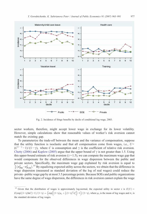
Fig. 2. Incidence of fringe benefits by decile of conditional log wage, 2003.
977Y. Gorodnichenko, K. Sabirianova Peter / Journal of Public Economics 91 (2007) 963–991
sector workers, therefore, might accept lower wage in exchange for its lower volatility.However, simple calculations show that reasonable values of worker's risk aversion cannotmatch the existing gap.
To parameterize the trade-off between the mean and the variance of compensation, supposethat the utility function is isoelastic and that all compensation come from wages, i.e., U=(C1− γ−1) / (1−γ), where C is consumption and γ is the coefficient of relative risk aversion.Chetty (2006) and Kaplow (2005) argue that the upper bound of γ is not greater than 1.5. Usingthis upper-bound estimate of risk aversion (γ=1.5), we can compute the maximum wage gap thatwould compensate for the observed differences in wage dispersion between the public andprivate sectors. Specifically, the maximum wage gap explained by risk aversion is equal tog2 ðr2PRI−r2PUBÞ.15 By equalizing expected utility across the sectors, we obtain that the difference inwage dispersion (measured as standard deviation of the log of real wages) could reduce theprivate–public wage gap by at most 3.5 percentage points. Because SOEs and public organizationshave the same degree of wage dispersion, the differences in risk aversion cannot explain the wage
15 Given that the distribution of wages is approximately log-normal, the expected utility in sector x is EðUÞ ¼Eðexpfð1−gÞlnCg−1Þ=ð1−gÞ ¼ exp ð1−gÞlx þ 1
2 ð1−gÞ2r2xn o
−1� �
=ð1−gÞ, where μx is the mean of log wages and σx is
the standard deviation of log wages.
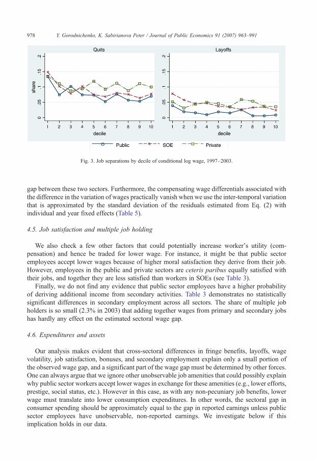
Fig. 3. Job separations by decile of conditional log wage, 1997–2003.
978 Y. Gorodnichenko, K. Sabirianova Peter / Journal of Public Economics 91 (2007) 963–991
gap between these two sectors. Furthermore, the compensating wage differentials associated withthe difference in the variation of wages practically vanish when we use the inter-temporal variationthat is approximated by the standard deviation of the residuals estimated from Eq. (2) withindividual and year fixed effects (Table 5).
4.5. Job satisfaction and multiple job holding
We also check a few other factors that could potentially increase worker's utility (com-pensation) and hence be traded for lower wage. For instance, it might be that public sectoremployees accept lower wages because of higher moral satisfaction they derive from their job.However, employees in the public and private sectors are ceteris paribus equally satisfied withtheir jobs, and together they are less satisfied than workers in SOEs (see Table 3).
Finally, we do not find any evidence that public sector employees have a higher probabilityof deriving additional income from secondary activities. Table 3 demonstrates no statisticallysignificant differences in secondary employment across all sectors. The share of multiple jobholders is so small (2.3% in 2003) that adding together wages from primary and secondary jobshas hardly any effect on the estimated sectoral wage gap.
4.6. Expenditures and assets
Our analysis makes evident that cross-sectoral differences in fringe benefits, layoffs, wagevolatility, job satisfaction, bonuses, and secondary employment explain only a small portion ofthe observed wage gap, and a significant part of the wage gap must be determined by other forces.One can always argue that we ignore other unobservable job amenities that could possibly explainwhy public sector workers accept lower wages in exchange for these amenities (e.g., lower efforts,prestige, social status, etc.). However in this case, as with any non-pecuniary job benefits, lowerwage must translate into lower consumption expenditures. In other words, the sectoral gap inconsumer spending should be approximately equal to the gap in reported earnings unless publicsector employees have unobservable, non-reported earnings. We investigate below if thisimplication holds in our data.
979Y. Gorodnichenko, K. Sabirianova Peter / Journal of Public Economics 91 (2007) 963–991
Because information on expenditures and assets is available at the household level, weaggregate our individual variables in Eq. (1) to the household level and estimate the followingbase wage equation for the 2003 household data:
lnwh ¼ b0 þ b1NSOEh þ b2N
PRIh þ b3N
OTHh þ b4N
EARh þ X hgþ eh; ð6Þ
where bars indicate that independent variables and errors are averaged across all wage earners inhousehold h; Xh include the same vector of covariates as in Eq. (1) aggregated at the householdlevel (i.e., years of schooling, gender, experience, experience squared, tenure, tenure squared,full-time job, firm size, and location); Nh
SOE, NhPRI, Nh
OTH denote the number of householdmembers employed in SOEs, private firms, and other sectors (collectives), respectively;16 andNh
EAR is the number of household wage earners. Households with no wage earners are excludedfrom the analysis.
We employ three definitions of labor compensation (wh): household total of individualmonthly contractual (accrued) wages at the primary job; total wages received last month by allhousehold members at their primary jobs; and total earnings in the form of money, goods, andservices received last month by all household members from their primary and secondary jobs.All wages and earnings are net of taxes. As shown in Table 6, all three estimated household wagefunctions are consistent with our previous findings and indicate a significant wage gap betweenthe public and non-public sectors. A marginal increase in total household earnings when amember is employed in the private sector instead of being employed in the public sector is 0.163–0.175 (0.102–0.124 for SOEs) log points, ceteris paribus. Sectoral differences in earnings arestatistically significant at the 1% level.
To make estimates in household income and consumption functions comparable, we need tomake one more step in aggregation of income measure, that is, we need to add the non-laborportion of household income. This will also require using finer controls for the householdcomposition, including the number of major contributors to non-labor income.
lnYh ¼ b0 þ b1NSOEh þ b2N
PRIh þ b3N
OTHh þ b4N
EARh þ b5N
HHMh þ X hgþ eh; ð7Þ
where Yh is total household income comprised of contractual monthly labor earnings from alljobs, accrued monthly pensions, and other types of income actually received last month (stipends,social payments, alimonies, income from capital investment, rental income, etc.); Nh
HHM is thevector of household composition variables such as the number of household members, thenumber of pensioners (the largest source of non-labor income), and the number of children15 years and younger. After adding non-labor income, the income premium associated withhousehold member working in the private sector and SOEs remains large and statisticallysignificant at the 1% level (0.135 and 0.104, respectively, as shown in Table 6).
Now we can replace the dependent variable in Eq. (7) with the measures of householdexpenditures and examine if there is a consumption gap across sectors in the following model:
lnCh ¼ b0 þ b1NSOEh þ b2N
PRIh þ b3N
OTHh þ b4N
EARh þ b5N
HHMh þ X hgþ eh; ð8Þ
16 Coefficients are easier to interpret when we use the number of the employed household members instead of theemployment shares. For example, β1 shows a marginal increase in household earnings if a household member isemployed in SOEs instead of being employed in a public organization. To have a complete account for householdearnings, we included workers in other sectors (collectives) in this part of the analysis.

Table 5Dispersion of wages
Panel A: dispersion of wages by year
1991 1997 1998 1999 2000 2001 2002 2003
Standard deviation of log of monthly wagePublic 0.480 0.553 0.539 0.533 0.511 0.495 0.512 0.473SOE 0.539 0.602 0.574 0.551 0.572 0.567 0.584 0.570Private 0.829 0.651 0.633 0.634 0.633 0.609 0.636 0.610
90–10 wage differentialsPublic 1.139 1.273 1.139 1.227 1.099 1.068 1.070 1.019SOE 1.358 1.322 1.358 1.308 1.310 1.427 1.357 1.386Private 1.792 1.609 1.492 1.609 1.526 1.466 1.455 1.386
Panel B: dispersion of wages in the pooled sample, 1997–2003
Standard deviation of log of monthly wage ΔWage gap
Public SOE Private SOE–public Private–public
Variation in lnwit (raw data adjusted for inflation)All 0.508 0.556 0.629 0.013 0.035Males 0.583 0.538 0.642 … 0.018Females 0.442 0.490 0.569 0.011 0.032
Variation in conditional lnwit (OLS residuals)All 0.427 0.471 0.570 0.010 0.036Males 0.518 0.492 0.597 … 0.022Females 0.387 0.446 0.524 0.012 0.032
Inter-temporal variation in conditional lnwit (FE residuals)All 0.259 0.303 0.281 0.006 0.003Males 0.273 0.317 0.284 0.007 0.002Females 0.255 0.289 0.277 0.005 0.003
Notes: ΔWage gap=the change in the wage gap that compensates the differences in the dispersion of wages between thesectors (γ=1.5). The dispersion of conditional log of monthly wage is computed on the basis of the OLS residuals obtainedfrom Eq. (1). Inter-temporal variation on conditional log wage is approximated by the standard deviation of residualsestimated from Eq. (2), with individual and year fixed effects included.
980 Y. Gorodnichenko, K. Sabirianova Peter / Journal of Public Economics 91 (2007) 963–991
where Ch is a measure of consumption expenditures. Table 6 provides the consumption gapestimates for durables, non-durables, and different subsets of consumer non-durables such as food(food, beverages, and tobacco), apparel, and services (transportation, health care, education,entertainment, and recreation). Regardless of the measure, we do not find significant differencesin expenditures of workers across sectors. At the same time the coefficients on other covariates aregenerally consistent with standard theoretical predictions. For example, Table 6 shows thatschooling has positive and statistically significant returns in almost all household income andexpenditure functions (except for durables).
In principle, workers with different level of true earnings could have comparable levels ofexpenditures if, for example, private sector employees save more (consume less) because oftheir job and wage uncertainty. Note that we focus on contractual wages rather than actualwages because contractual wages are less affected by transitory income shocks and thus canserve as a proxy for permanent income. We have also shown that the sectoral differences in job
981Y. Gorodnichenko, K. Sabirianova Peter / Journal of Public Economics 91 (2007) 963–991
uncertainty and wage volatility are so small (see Section 4.4) that they are unlikely to inducesavings in the private sector sufficient to equalize expenditures. Indeed, we find that householdswith workers in the private sector do not hold more assets (accumulated savings) thanhouseholds with public sector workers.17 Table 6 reports that employees in the private andpublic sectors have an essentially identical probability of possessing cars, phones, cell phones,and computers, and they live in better housing conditions (with higher market value and largertotal living space) than households with SOEs workers. Hence the precautionary motives ofworkers cannot reconcile the sizeable sectoral gap in wages with the minor gap in expendituresand assets.18
The same set of controls in both the income Eq. (7) and the consumption Eq. (8) allows us tosubtract one equation from another and estimate the consumption–income gap directly asfollows:
lnCh−lnYh ¼ b0 þ b1NSOEh þ b2N
PRIh þ b3N
OTHh þ b4N
EARh þ b5N
HHMh þ X hgþ eh; ð9Þ
where Ch is expenditures on non-durables, Yh is total household income, lnCh− lnYh is theconsumption–income gap (or “C–Y gap”), and all other variables are defined as above.19 Animportant property of this specification is that it controls for any unobservable householdcharacteristics that are omitted and simultaneously affect household income and consumption.Most likely the estimates of Eq. (9) understate the extent of the consumption–income gap in thepublic sector because workers in SOEs and the private sector are likely to receive unofficial non-taxable compensation (“payments in envelopes”).20 In line with the estimates of income andconsumption functions, we find that the consumption income gap in the public sector iseconomically and statistically significant, and it is 7.2–7.3% greater than in the two other sectors(Table 6).
4.7. Bribery
Our findings clearly suggest that the sectoral differences in expenditures and asset holdings areconsiderably smaller than the sectoral differences in wages. Thus, we cannot attribute the largeprivate–public wage gap in Ukraine to the differences in non-pecuniary job amenities such as jobsecurity, fringe benefits, job satisfaction, efforts, etc. The similar levels of consumer expendituresacross sectors unambiguously indicate that public sector employees receive unobserved monetary
17 We also find that public sector workers are no more likely to have debts for utility payments than employees in othersectors. These utility debts are one of the largest sources of credit to individuals since the consumer credit market is notdeveloped in Ukraine.18 In the associated working paper (Gorodnichenko and Sabirianova Peter, 2006), we test the “elite hypothesis” andshow that the coefficient on private ownership is not likely to be biased downwards in the asset and consumptionfunctions if members of wealthy families are more likely to get a job in the public sector.19 Alternatively we estimated Eqs. (6)–(9) with controls that characterize the household head (defined as the person withlargest earnings). The results are reported in the associated working paper. They are very similar to the specifications thatuse controls averaged for household wage earners.20 Estimates from Eq. (9) can overstate the consumption–income gap if public sector employees (1) systematically saveless, (2) systematically spend less on durables, or (3) have greater complementarity in consumption and leisure thanworkers in other sectors. These cases, however, contradict to the equality of asset holdings (wealth) and consumption ofnon-durables across sectors that we found previously.

Table 6Household income, expenditures, and wealth, 2003
Dependentvariables:
SOE sector Private sector No. of earners Schooling Mean (sd) N
(1) (2) (4) (5) (6) (7)
Household incomeContractual wage 0.118⁎⁎⁎ 0.166⁎⁎⁎ 0.532⁎⁎⁎ 0.051⁎⁎⁎ 420.7 2272
/OLS/ (0.022) (0.023) (0.022) (0.004) (313.9)Actual wage 0.102⁎⁎⁎ 0.163⁎⁎⁎ 0.511⁎⁎⁎ 0.048⁎⁎⁎ 414.6 2180
/OLS/ (0.023) (0.024) (0.024) (0.005) (317.2)Total earnings 0.124⁎⁎⁎ 0.175⁎⁎⁎ 0.283⁎⁎⁎ 0.055⁎⁎⁎ 497.3 2081
/OLS/ (0.029) (0.031) (0.030) (0.006) (391.1)Household income 0.104⁎⁎⁎ 0.135⁎⁎⁎ 0.434⁎⁎⁎ 0.041⁎⁎⁎ 526.5 2202
/OLS/ (0.021) (0.022) (0.022) (0.004) (337.3)
ExpendituresNon-durables 0.019 0.057 0.087⁎⁎ 0.038⁎⁎⁎ 623.2 2000
/OLS/ (0.036) (0.038) (0.038) (0.007) (765.2)Food 0.026 0.050 0.073⁎ 0.028⁎⁎⁎ 87.9 2066
/OLS/ (0.036) (0.038) (0.038) (0.007) (82.8)Apparel 0.053 0.027 −0.007 0.025⁎⁎ 185.8 1184
/OLS/ (0.060) (0.063) (0.063) (0.013) (200.8)Services 0.003 0.055 0.119⁎⁎ 0.066⁎⁎⁎ 190.9 2034
/OLS/ (0.052) (0.055) (0.055) (0.010) (600.2)Durables, annual 0.170 −0.118 −1.081 0.315 2957.1 2234
/Tobit/ (0.977) (1.033) (1.037) (0.192) (5976.0) [241]
Consumption–income gapC–Y gap −0.072⁎⁎ −0.073⁎⁎ −0.345⁎⁎⁎ −0.003 0.045 1949
/OLS/ (0.035) (0.037) (0.037) (0.007) (0.800)
Household assets/debtValue of housing −0.645⁎⁎⁎ −0.377 0.552⁎⁎ 0.187⁎⁎⁎ 8508.5 1337
/Tobit/ (0.244) (0.252) (0.253) (0.050) (9340.0) [1092]Housing space −2.373⁎⁎ −0.550 −0.291 0.424⁎⁎ 60.6 2047
/OLS/ (1.067) (1.118) (1.117) (0.214) (25.1)Debt for utilities 0.266 0.668 −0.263 0.094 776.3 2223
/Tobit/ (0.392) (0.409) (0.412) (0.078) (1169.6) [736]Computer 0.003 0.019⁎⁎ −0.003 0.017⁎⁎⁎ 0.073 2264
/Probit/ (0.009) (0.010) (0.009) (0.002) (0.261)Phone −0.027 −0.017 0.035 0.056⁎⁎⁎ 0.528 2269
/Probit/ (0.024) (0.025) (0.025) (0.006) (0.499)Cell 0.005 0.014 −0.008 0.014⁎⁎⁎ 0.090 2263
/Probit/ (0.012) (0.012) (0.013) (0.002) (0.286)Car −0.031 −0.027 0.014 0.024⁎⁎⁎ 0.237 2269
/Probit/ (0.019) (0.020) (0.020) (0.004) (0.425)
Notes: Household is the unit of observation. Except for tobit, robust standard errors are in parentheses; ⁎ significant at10%; ⁎⁎ significant at 5%; ⁎⁎⁎ significant at 1%. In tobit specifications zero values are replaced by 1, observations withlog(depvar) N0 are in brackets and their conditional mean is reported in column 6. To reduce the influence of outliers inearnings and consumption functions, the OLS is performed as a Huber robust regression, with lower weights given toinfluential observations. All income and expenditures measures are used in logarithmic form. All specifications includeindividual covariates from Eq. (1) that are averaged for household wage earners. Specifications related to the wholehousehold (as opposed to the first three specifications for wage earners) also include controls for household compositionsuch as number of household members, number of children, and number of retirees. The consumption–income gap (C–Ygap) is defined in the text.
982 Y. Gorodnichenko, K. Sabirianova Peter / Journal of Public Economics 91 (2007) 963–991

983Y. Gorodnichenko, K. Sabirianova Peter / Journal of Public Economics 91 (2007) 963–991
compensation that allows them to enjoy the level of consumption comparable to the consumptionof workers in the other sectors. We refer to this unobserved, non-reported compensation as abribe.
By its nature, bribery is unobserved (or at least unreported by bribe receivers) and, hence, thehypothesis that bribes explains the wage gap cannot be tested directly. However, we can test thebribery hypothesis indirectly by examining the variation of the consumption–income gap acrossoccupations and subsectors of the public sector. It has been found by Mocan (2004), Hunt (2005),and others that certain occupations and subsectors of the public sector are more prone tocorruption than others. For example, 73% of the respondents in the recent survey of corruptionin Ukraine indicated they had offered money to medical workers (Woronowycz, 2003). Like-wise, the incidence of corruption appears to be very high in enforcement agencies and publicadministration.
Earlier we have shown that the wage gap is the largest among the highly paid workers whomay extort larger side payments because of either their high positions within the governmenthierarchy or ability to provide better services (e.g., high-quality physicians). Now we canextend this analysis further by allowing the consumption–income gap in Eq. (9) to varyacross major occupational groups and subsectors (such as public administration, education,health care and social work, and other industries which include army and public organizationsin arts, culture, and science).21 If the bribery hypothesis holds, then the groups that com-monly perceived as bribe takers should display larger positive discrepancy between con-sumption and income. To avoid the plethora of dummy variables for each householdmember (interacted with occupations and subsectors), we use characteristics of the head of thehousehold in Eq. (9).22 The results are reported in Table 7, with the private sector as anomitted category.
Consistent with the predictions of the bribery hypothesis, we find that the largestconsumption–income gap is observed in public administration (including police, customs,and tax authorities) and health care (which also includes social work). The consumption–income gap is 0.238 and 0.247 log points respectively larger when compared to the gap in theprivate sector. Table 7 also provides two specifications with occupations: column (3) com-pares typical occupations in the public sector with all occupations in the private sectorassuming skill transferability (public sector workers might choose a different occupationwhen they move to the private sector); and column (4) compares occupations in the publicsector with the same occupations in the private sector assuming skill non-transferability. Inboth cases we see the gap is larger for public sector managers (0.247 log points) and healthcare professionals and associate professionals (0.226 log points). These occupations andsubsectors provide services that have highly inelastic demand and, thus, create the greatestopportunities to extract bribes.
In addition to these formal tests, the bribery hypothesis is consistent with many other pieces ofevidence. Indeed, numerous media reports and surveys indicate widespread bribery in theUkrainian public sector. Ukraine is persistently at the bottom of the world distribution of theTransparency International Corruption Perceptions Index. Ukraine was ranked 69–70 among 85
21 Further breakdown of the public sector cannot be done with these data because finer disaggregation leads to having afew observations per cell.22 We thank a referee for suggesting this specification. The results are similar if we control with average householdcharacteristics.

Table 7The consumption–income gap by subsector and major occupational group of the public sector, head of householdspecification, 2003
(1) (2) (3) (4)
Private sector — all occupations Omitted Omitted Omitted …Public sector — all occupations 0.118⁎⁎
(0.048)Public sector by subsector:
Public administration 0.238⁎⁎
(0.107)Healthcare 0.247⁎⁎⁎
(0.073)Education 0.043
(0.065)Other public sector industries −0.086
(0.106)Public sector by occupation:
Managers 0.247⁎⁎ 0.244⁎⁎
(0.120) (0.120)Health professionals and associates 0.226⁎⁎⁎ 0.225⁎⁎⁎
(0.086) (0.086)Teaching professionals and associates 0.017 0.015
(0.080) (0.081)Other public sector occupations 0.102 0.101
(0.064) (0.065)Private sector by occupation:
Managers 0.023(0.091)
Health professionals and associates −0.366(0.284)
Teaching professionals and associates 0.376(0.692)
Other private sector occupations OmittedSOE 0.006 0.006 0.007 0.006
(0.038) (0.037) (0.038) (0.038)Other sectors −0.139⁎⁎ −0.139⁎⁎ −0.139⁎⁎ −0.140⁎⁎
(0.068) (0.068) (0.068) (0.068)
Notes: N=1938. Household is the unit of observation. Household head is the person with largest earnings. Robust standarderrors are in parentheses; ⁎ significant at 10%; ⁎⁎ significant at 5%; ⁎⁎⁎ significant at 1%. To reduce the influence ofoutliers in earnings and consumption functions, the OLS is performed as a Huber robust regression, with lower weightsgiven to influential observations. All specifications include individual covariates for the household head from Eq. (1) andcontrols for household composition such as number of household members, number of children, and number of retirees.The dependent variable – consumption–income gap – is defined in the text.
984 Y. Gorodnichenko, K. Sabirianova Peter / Journal of Public Economics 91 (2007) 963–991
surveyed countries in 1998, 87–88 among 90 countries in 2000, and 122 among 146 countries in2004 (Transparency International, 2005). Pervasive and persistent bribery in Ukraine is consistentwith the positive and time-invariant private–public wage gap.
5. Measuring bribery
In this section, we use the equalizing differences framework to obtain an estimate of bribery atthe country level. In a labor market with unconstrained entry and exit, equilibrium is achieved

985Y. Gorodnichenko, K. Sabirianova Peter / Journal of Public Economics 91 (2007) 963–991
when the total worker compensation is equalized across sectors.23 In this framework bribery, aswith any other form of non-labor compensation, is going to be reflected in compensating wagedifferentials across sectors. There are three underlying assumptions to this method: there is nobribery in the private sector, there are no queues in the public sector, and there is no risk of beingdetected taking bribes. If private sector employees receive bribes (e.g. for utility repairs, phoneinstallation, etc.), then our estimate of aggregate bribery is going to be understated. If there areentry constraints in the public sector (in the form of queues or bribes to get a job in the publicsector), then our bribery measure is also going to be understated because any additional investmentin acquiring a job in the public sector will result in higher reservation wage, longer job tenure, andfewer quits in the public sector.24 We find that voluntary turnover in the public sector is no less thanin the other sectors, and tenure in public organizations is no longer than in SOEs (Tables 3 and A2).Thus, entry constraints do not appear to be important in Ukraine. If there is a significant risk ofbeing detected (which is likely to be low in a country where bribe is a social and acceptable norm),then workers in the public sector should demand higher bribes to compensate for the risk.
In our calculations we ignore general equilibrium effects, which, however, are likely to amplifythe magnitude of bribery. Since in equilibrium after-tax compensation in the public and privatesectors is equalized, it must hold, ceteris paribus, that
Wp ¼ Wbð1þ bÞ; ð10ÞwhereWb is average annual after-tax earnings in the public sector,Wp is annual after-tax earningsin the private sector, and β is the proportion of annual earnings received in the form of bribes bythe average worker in the public sector. Because current wage is the best predictor of future wagesand of the net present value of wage stream, this condition also applies to life-time earnings.
Thus, the total amount of bribes in the public sector (B) is equal to NbWbβ, where Nb is thenumber of employees in the public sector. The corresponding formula for the amount of bribesusing the hourly wage rate is Nbwbhbβ, where wb is the average after-tax hourly wage in the publicsector and hb is annual hours of work in the public sector.
In these calculations it is assumed that the wage gap β is the same for all workers. However,our quantile estimates suggest that the wage gap is increasing with the level of conditional wage.We can account for this fact by weighting the estimated wage gap in each percentile (βθ) by thecorresponding level of wage (wbθ):
B ¼ Nbhb1
100
X100
h¼1
wbhbh; ð11Þ
where θ is the θth percentile of the wage distribution.
23 Even if the employer sets the wage (which is a quite plausible assumption given that trade unions are very weak inUkraine), it is the workers who move across sectors and eliminate arbitrage opportunities. If the private sector employeespersistently receive larger rents (due to “efficiency wage” policies), then we would observe lower exit rates and longertenure in the private sector, which we do not see in our data. The similar rates of voluntary separations in the private andpublic sectors contradict to the efficiency wage argument and may be also taken as evidence that arbitrage opportunitiesare eliminated in the labor market.24 Several studies indicate higher wages in the public sector in countries with relatively high corruption (Terrell (1993)for Haiti and Nielsen and Rosholm (2001) for Zambia). In these countries bribery is likely to appear on the quantity sidein the form of queues or side payments to get a job in the public sector.

Table 8Estimates of bribery in the public sector, 2003
Method Wagegapestimate
Aggregate bribery
Million UAH % of GDP % of wage bill
SOE vs. publicUnconditional monthly wage, 2003 0.286 4132 1.56 6.36OLS, monthly wage, 1997–2003 0.153 2063 0.78 3.18Fixed effect, monthly wage, 1997–2003 0.125 1662 0.63 2.56Individual-specific trend, monthly wage, 1997–2003 0.165 2239 0.85 3.45OLS, hourly wage, 2003 0.160 2165 0.82 3.33OLS, expected hourly wage, 2003 0.153 2063 0.78 3.18Quantile regression, hourly wage, 2003 0.185 2542 0.96 3.91Quantile regression, expected hourly wage, 2003 0.178 2438 0.92 3.75
Private vs. publicUnconditional monthly wage, 2003 0.304 4434 1.68 6.82OLS, monthly wage, 1997–2003 0.249 3528 1.34 5.43Fixed effect, monthly wage, 1997–2003 0.214 2978 1.13 4.58Individual-specific trend, monthly wage, 1997–2003 0.279 4016 1.52 6.18OLS, hourly wage, 2003 0.193 2657 1.01 4.09OLS, expected hourly wage, 2003 0.178 2431 0.92 3.74Quantile regression, hourly wage, 2003 0.238 3346 1.27 5.15Quantile regression, expected hourly wage, 2003 0.221 3094 1.17 4.76
Notes: The amount of bribes is computed according to the methodology described in Section 6. In addition to the estimatedwage gap, we also use the following data for 2003: GDP=264,165 million UAH; Nb=3,741 million people, averagebefore-tax monthly wage of the public sector employee=351 UAH; total wage bill=64,966 million UAH, effectiveincome tax rate=20.8% (State Statistics Committee of Ukraine, 2003). The wage gap estimate for quantile regressions is aweighted average across percentiles, with conditional hourly wage rate used as a weight.
986 Y. Gorodnichenko, K. Sabirianova Peter / Journal of Public Economics 91 (2007) 963–991
Since β is not observed, we use the estimate of β from Eqs. (1)–(5) to compute the proportionof annual earnings received in bribes as (exp( β )−1). Table 8 shows the aggregate measures ofbribery in the public sector in 2003 for several alternative estimates of β.25
The range of the estimated amount of bribes in the public sector is rather large — from1662 million UAH to 4434 million UAH. As previous analysis indicated, some estimates arebetter than others. Conditional wage gap estimates are superior to unconditional ones forthe obvious reason of accounting for the differences in worker characteristics. We areindifferent between the various panel data estimates because they are close to each other anddistributed compactly around the pooled OLS estimate. We prefer hourly wage over monthlywage since it allows us to control for the sectoral difference in hours of work. We wouldchoose expected hourly wage over actual hourly wage in order to account for the difference injob security. The quantile estimates are superior to the OLS estimates in computing briberybecause they give more weights to high earners who are likely to extract larger bribes. We use
25 To compute the amount of bribes, we use the following data for 2003: GDP=264,165 million UAH; Nb=3741 millionpeople, average before-tax monthly wage of the public sector employee=351 UAH; total wage bill = 64,966 millionUAH; effective income tax rate (to compute after-tax monthly wage) =20.8% (State Statistics Committee of Ukraine,2003).

987Y. Gorodnichenko, K. Sabirianova Peter / Journal of Public Economics 91 (2007) 963–991
both SOE–public and private–public gap measures to define the range of our preferredbribery estimates.26
Based on our preferred wage gap estimates, the amount of bribery in the public sector inUkraine equals 2438–3094 million UAH (457–580 million U.S. dollars), which translates into0.9–1.2% of GDP and 3.8–4.8% of the total wage bill in the economy. This estimate is likely tobe a lower bound because of potential bribery in the private sector, soft budget constraints in thepublic sector, non-profit objective function of public organizations, larger bonuses in SOEs andprivate firms, etc. Even though this lower bound estimate is large, we believe it is entirelyplausible. According to various estimates, the size of the shadow (unofficial) economy in Ukraineis at least 30% of GDP (Johnson et al., 2000; Schneider and Enste, 2000). Suppose that the publicsector employees extract bribes by allowing the activity of the shadow economy, then theeffective tax rate on the shadow economy would be about 4% (=1.2% GDP in bribes divided bythe size of the shadow economy (30% of GDP)). In contrast, the tax burden on the official sector ismuch higher (the value added tax alone is 20%) and, thus, bribery can be a profitable mechanismof tax evasion.
6. Conclusions
Our analysis provides the first systematic measure of bribery using micro-level data onobservable labor market outcomes, household spending, and asset holdings. Bribery is a socialscourge in developing and transition countries. However, available estimates of bribery arequalitative and subjective. We show how one can obtain a simple and robust estimate of briberyfrom income, expenditures and asset holdings data. Specifically, we use the compensatingdifferential framework and the estimated sectoral gap in expenditures and reported earnings toidentify the size of unobserved (unofficial) compensation (i.e., bribes) of public sectoremployees. Using the conditions of labor market equilibrium, we offer a technique to calculatean aggregate measure of bribery in a country or a sector. Since we make only a few assumptions,our method should be practically helpful in welfare calculations and designing anti-corruptionpolicies throughout the world.
In the case of Ukraine, we find that public sector employees receive on average 24–32% less inmonthly wages than their private sector counterparts and that the size of the wage gap does notdiminish over time. The gap remains large after controlling for a number of covariates and time-invariant unobservable worker characteristics. We also find that the private–public wage gap ispositive at all percentiles of the conditional wage distribution, and it increases with workerproductivity, reaching 67.5% in the 90th percentile of the wage distribution. All of these empiricalobservations are consistent with pervasive bribery in Ukraine.
We attribute the significant portion of the observed differences in reported earnings to bribes(20–27% of public sector wages). Our analysis of household expenditures and asset holdingsallows us to conclusively rule out theories that lower wages of public worker employees are offsetby non-pecuniary characteristics of a public sector job such as efforts, fringe benefits, jobsatisfaction, job security, etc. We strengthen our analysis by examining a better counterfactual(SOEs) for the public sector. We find that large sectoral differences in wages are not translated into
26 SOEs and public organizations share a lot of similarities in terms of the variance of wages, hours of work, fringebenefits and many other characteristics; and, for that reason, public employees might consider working in SOEs as abetter alternative than working in the private sector.

988 Y. Gorodnichenko, K. Sabirianova Peter / Journal of Public Economics 91 (2007) 963–991
comparable differences in the levels of consumer expenditures and wealth as employees in thepublic and private sectors enjoy similar levels of consumption. We show that corruption proneoccupations and subsectors of the public sector have the largest discrepancy between consumptionand income, thus supporting our explanation of the wage gap being driven by bribes.
Using a no-arbitrage argument, we develop an aggregate measure of bribery and find thatthe lower bound estimate of the extent of bribery in Ukraine is between 460 million and580 million U.S. dollars, which is equivalent to 0.9–1.2% of Ukraine's GDP and 3.8–4.8% ofthe official wage bill in 2003. Hence, at least 1% of GDP should be allocated to ensuring fairwages in the public sector. Given that the wage gap is particularly large at the top of the wagedistribution, the decompression of wages in the public sector might be a necessary prescriptionfor reducing corruption at the top levels. Although ensuring fair wages in the public sector isnecessary in reducing corruption, it is not a sufficient condition and should be complementedwith other measures such as increasing transparency and competition in the public sector,improving accountability and enforcement, etc. that reduce the incentives and powers to extractbribes.
We believe that combining expenditures/asset and income data is a fruitful avenue in theanalysis of the private–public wage differentials. Since household budget surveys are availablefor many countries, our analysis can be easily replicated in other transition and developingcountries where bribery is present.
Acknowledgement
The authors would like to thank David Brown, John Earle, Bruce Kaufman, Patrick Kline, JanSvejnar, anonymous referees, seminar participants at the Georgia State University, University ofKentucky, University of Michigan, and the participants at the ACES/ASSA Meetings inPhiladelphia and Boston, the IZA/World Bank conference “Employment and Development” inBerlin, and the Econometric Society European Meetings in Vienna for useful comments.Sabirianova Peter acknowledges the research support from the National Council for Eurasian andEast European Research and the NSF (Research Grant SES 0111783).
Appendix A
Table A1Definitions of variables
Variable
DescriptionPublic
=1 if primary employer is a budgetary organization SOE =1 if primary employer is a state enterprise or a local municipal enterprise Private =1 if primary employer is a privatized enterprise, a newly established private enterprise; or aforeign company
Wage Monthly contractual wage after taxes at the primary job in December of the corresponding year. Allwages are converted into hryvnyas.
Adjusted yearsof schooling
Education status from the survey has been converted into a continuous variable representing adjustedyears of schooling. Adjusted years of schooling were taken as 4 for 1–6 grades, 8 for 7–9 grades, 10 for10–12 secondary school grades, 9 for a vocational non-secondary school diploma, 11.5 for a vocationalsecondary school diploma, 13 for a technical school diploma and incomplete higher education, 14 for abachelor degree, 15 for a diploma of specialist, 16 for a master degree, and 18 for a Ph.D. degree. Samedefinitions are used to compute adjusted years of schooling of parents.Female
=1 if female
989Y. Gorodnichenko, K. Sabirianova Peter / Journal of Public Economics 91 (2007) 963–991
(continued)Table A1 (continued )
Variable
DescriptionExperience
Age minus years of schooling minus 6 Tenure Number of years since an individual started the primary job Full-time job =1 if worked full time throughout a given year Weekly hours ofwork
2003: hours per week an individual usually works at the primary job; not available for other yearsFirm size
Number of persons working at enterprise (workplace for self-employed) of primary job: 1–9, 10–49,50–99, 100–499, 500–999, 1000+, and no informationRegions
5 regional dummies: Eastern, Southern, Western, Central and Northern, and Kyiv city Fringe benefits 2003: 14 categorical variables for various types of fringe benefits at the primary job; not availablefor other years
Bonuses Several dummies indicating whether an employee received the following types of bonuses last year:13th salary, performance-based bonus, bonus for work conditions, profit sharing, or other bonuses.
Job separations Two dummies indicating whether an individual is laid off or quits during the next year. Job satisfaction Categorical variable that ranges from 1 (fully unsatisfied) to 5 (fully satisfied) Secondary job =1 if had a secondary job during the reference week Total earnings After tax total earnings in the form of money, goods, and services received last month by allhousehold members from their primary and secondary jobs.
Householdincome
After tax sum of contractual monthly labor earnings from all jobs, accrued monthly pensions, and othertypes of income actually received last month (stipends, alimonies, unemployment insurance, child caresubsidies, income from capital investment, rental income, etc.)Non-durables
Last month expenditures on food, beverages, tobacco, apparel, and services (including transportation,health care, education, and entertainment); all weekly food expenses are multiplied by 4.Durables
Last year expenditures on furniture, refrigerator, washer/dryer, car, truck, motorcycle, summer house,plot, and house/apartment.Assets
Four dummy variables indicating whether a household possesses a car, a phone, a cell phone,or a computer.Value of housing
Self-estimated current market value of housing. Debt for utilities Amount of accumulated unpaid bills for utilities. Housing space Total area of the residence, m2.Table A2Summary statistics, 2003
Males
FemalesPublic
SOE Private Public(
SOE
continued on n
Private
Distribution by sector
0.106 0.402 0.491 0.313 0.339 0.348 Schooling (adjusted years) 14.032 12.450 12.267 13.580 12.710 12.653(3.257)
(2.345) (2.349) (2.393) (2.439) (2.407) Experience (years) 21.836 21.067 19.431 21.031 23.603 19.597(10.936)
(10.968) (11.665) (10.452) (10.386) (10.603) Tenure (years) 8.971 9.825 7.359 11.571 12.515 8.183(8.488)
(9.194) (8.942) (9.219) (10.082) (9.470) Average hours per week 41.130 41.810 44.198 37.495 39.234 44.839(10.824)
(8.703) (10.556) (9.361) (9.151) (13.306) Full-time job 0.971 0.973 0.952 0.909 0.916 0.941 Firm size (no. of persons)1–9
0.044 0.029 0.115 0.076 0.092 0.242 10–49 0.272 0.128 0.229 0.312 0.235 0.239 50–99 0.177 0.126 0.115 0.223 0.125 0.095 Size is missing 0.110 0.085 0.110 0.062 0.076 0.076 100–499 0.243 0.268 0.204 0.223 0.217 0.158ext page)
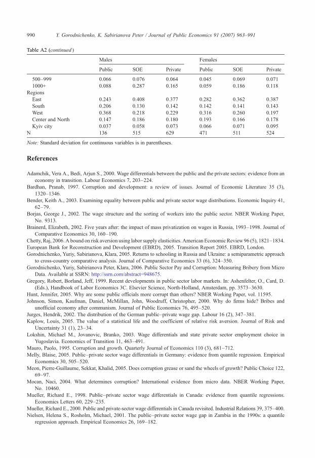
990 Y. Gorodnichenko, K. Sabirianova Peter / Journal of Public Economics 91 (2007) 963–991
(continued)Table A2 (continued )
Males
FemalesPublic
SOE Private Public SOE Private500–999
0.066 0.076 0.064 0.045 0.069 0.071 1000+ 0.088 0.287 0.165 0.059 0.186 0.118Regions
East 0.243 0.408 0.377 0.282 0.362 0.387 South 0.206 0.130 0.142 0.142 0.141 0.143 West 0.368 0.218 0.229 0.316 0.260 0.197 Center and North 0.147 0.186 0.180 0.193 0.166 0.178 Kyiv city 0.037 0.058 0.073 0.066 0.071 0.095N
136 515 629 471 511 524Note: Standard deviation for continuous variables is in parentheses.
References
Adamchik, Vera A., Bedi, Arjun S., 2000. Wage differentials between the public and the private sectors: evidence from aneconomy in transition. Labour Economics 7, 203–224.
Bardhan, Pranab, 1997. Corruption and development: a review of issues. Journal of Economic Literature 35 (3),1320–1346.
Bender, Keith A., 2003. Examining equality between public and private sector wage distributions. Economic Inquiry 41,62–79.
Borjas, George J., 2002. The wage structure and the sorting of workers into the public sector. NBER Working Paper,No. 9313.
Brainerd, Elizabeth, 2002. Five years after: the impact of mass privatization on wages in Russia, 1993–1998. Journal ofComparative Economics 30, 160–190.
Chetty, Raj, 2006.A bound on risk aversion using labor supply elasticities. American EconomicReview 96 (5), 1821–1834.European Bank for Reconstruction and Development (EBRD), 2005. Transition Report 2005. EBRD, London.Gorodnichenko, Yuriy, Sabirianova, Klara, 2005. Returns to schooling in Russia and Ukraine: a semiparametric approach
to cross-country comparative analysis. Journal of Comparative Economics 33 (6), 324–350.Gorodnichenko, Yuriy, Sabirianova Peter, Klara, 2006. Public Sector Pay and Corruption: Measuring Bribery from Micro
Data. Available at SSRN: http://ssrn.com/abstract=948675.Gregory, Robert, Borland, Jeff, 1999. Recent developments in public sector labor markets. In: Ashenfelter, O., Card, D.
(Eds.), Handbook of Labor Economics 3C. Elsevier Science, North-Holland, Amsterdam, pp. 3573–3630.Hunt, Jennifer, 2005. Why are some public officials more corrupt than others? NBER Working Paper, vol. 11595.Johnson, Simon, Kaufman, Daniel, McMillan, John, Woodruff, Christopher, 2000. Why do firms hide? Bribes and
unofficial economy after communism. Journal of Public Economics 76, 495–520.Jurges, Hendrik, 2002. The distribution of the German public–private wage gap. Labour 16 (2), 347–381.Kaplow, Louis, 2005. The value of a statistical life and the coefficient of relative risk aversion. Journal of Risk and
Uncertainty 31 (1), 23–34.Lokshin, Michael M., Jovanovic, Branko, 2003. Wage differentials and state private sector employment choice in
Yugoslavia. Economics of Transition 11, 463–491.Mauro, Paolo, 1995. Corruption and growth. Quarterly Journal of Economics 110 (3), 681–712.Melly, Blaise, 2005. Public–private sector wage differentials in Germany: evidence from quantile regression. Empirical
Economics 30, 505–520.Meon, Pierre-Guillaume, Sekkat, Khalid, 2005. Does corruption grease or sand the wheels of growth? Public Choice 122,
69–97.Mocan, Naci, 2004. What determines corruption? International evidence from micro data. NBER Working Paper,
No. 10460.Mueller, Richard E., 1998. Public–private sector wage differentials in Canada: evidence from quantile regressions.
Economics Letters 60, 229–235.Mueller, Richard E., 2000. Public and private-sector wage differentials in Canada revisited. Industrial Relations 39, 375–400.Nielsen, Helena S., Rosholm, Michael, 2001. The public–private sector wage gap in Zambia in the 1990s: a quantile
regression approach. Empirical Economics 26, 169–182.

991Y. Gorodnichenko, K. Sabirianova Peter / Journal of Public Economics 91 (2007) 963–991
Poterba, James M., Rueben, Kim S., 1994. The distribution of public sector wage premia: new evidence using quantileregression methods. NBER Working Paper, No. 4734.
Prescott, David, Wandschneider, Bo, 1999. Public–private sector wage differentials in Canada: evidence from 1991 and1982 surveys of consumer finance. Applied Economics 31, 723–731.
Schneider, Friedrich, Enste, Dominik H., 2000. Shadow economies: size, causes and consequences. Journal of EconomicLiterature 38 (1), 77–114.
Shleifer, Andrei, Vishny, Robert, 1993. Corruption. Quarterly Journal of Economics 108 (3), 599–617.State Statistics Committee of Ukraine, 2003. Yearbook of Ukraine. State Statistics Committee, Kyiv.Terrell, Katherine, 1993. Public–private wage differentials in Haiti: do public servants earn a rent? Journal of Development
Economics 42, 293–314.Transparency International, 2005. Annual Report 2004.van Ophem, Hans, 1993. A modified switching regression model for earnings differentials between the public and private
sectors in the Netherlands. Review of Economics and Statistics 75, 215–224.van Rijckeghem, Caroline, Weder, Beatrice, 2001. Bureaucratic corruption and the rate of temptation: do wages in the civil
service affect corruption, and by how much? Journal of Development Economics 65, 307–331.Woronowycz, Roman, 2003. Nationwide survey reveals culture of corruption in Ukraine. The Ukrainian Weekly 4 (71)
(January 26).