economies

Article

Public Transit Ridership and Car-Oriented Cities: TheCase of the Dallas Region

Ahmed Daqrouq and Ardeshir Anjomani *

Department of Planning and Landscape Architecture, College of Architecture, Planning and Public Affairs,University of Texas at Arlington, Arlington Texas, TX 76019, USA* Correspondence: anjomani@uta.edu

Received: 23 June 2019; Accepted: 19 August 2019; Published: 27 August 2019�����������������

Abstract: U.S. cities have invested large amounts of sums on public transit and urban rail in the lastfew decades, but the transit usage in most of these car-oriented cities is very low, and previous effortsto increase ridership have been mostly fruitless. This research examines the factors affecting transitridership in a large car-oriented metropolitan setting and uses the Dallas region in the United States asa case for the study to identify factors that could help in increasing ridership. Most previous studiesof transit ridership have not included many of the variables thought to influence transit ridership.Therefore, the disparities among the findings of empirical research completed to date point to thenecessity for further study. This study addresses these shortcomings by exploring multiple factors,measuring population, technology, geography, and socioeconomic characteristics.

Keywords: transit ridership; rail transit; bus transit; Dallas Area Rapid Transit (DART); intelligenttransit information systems (ITIS)

1. Introduction

Transit ridership is at the heart of transportation policy-making and the success of any transitsystem. In recent years, the energy component of transportation is becoming more apparent. NorthAmerica greatly depends on large amounts of cheap energy to keep its economy growing. The price ofenergy, especially fossil fuels, has been rising in recent years, and the price will likely continue to rise.This rise in energy price will mean that North America must adapt, as energy gets more expensiveand scarcer. One of the areas of adaptations needs to be made in transportation, as transportationconsumes large quantities of energy. Recent studies estimate that a large percentage of air pollutants isgenerated by the transportation sector. In 2017, transportation accounted for the largest portion (29%)of total U.S. GHG emissions, 82% of which derive from road transport (Fast Facts 2019). The transportsector currently accounts for 54% of the total oil consumption (EIA 2018). The number of cars isexpected to double by 2035 when their total number reaches 1.7 billion. This rise is mainly related tothe development of emerging economies like China, India, and the Middle East. Also, the expectedincrease in urbanization is likely to cause severe congestion problems in the next decades in most citiesall over the world (Borghesi et al. 2014).

Transit ridership is essential for policymaking and the success of any transportation system.Automobile dependence is a concern for many reasons, including congestion in urban areas, pollution,and environmental damages caused by pollution. Public transit is an efficient means to move largenumbers of people within cities, and transit systems play an important role in combating trafficcongestion, reducing carbon emissions, and promoting compact, sustainable urban communities(Taylor et al. 2009). This study will examine transit ridership in the Dallas metropolitan area as anexample of a quintessential car-oriented metro area in the United States. It will examine the factorsaffecting transit ridership in a case study applied to the Dallas Area Rapid Transit (DART), a regional

Economies 2019, 7, 86; doi:10.3390/economies7030086 www.mdpi.com/journal/economies

Economies 2019, 7, 86 2 of 17

transit agency in the Dallas metropolitan in Texas, as a sample of large low-density car-oriented citiesin the United States for a ten-year period of monthly data. We also include a measure of auto ridershipin the models in order to measure the responsiveness of demand for transit to a relative change in autousage. Also, as part of these factors, it explores the impact of intelligent transit information systems(ITIS) on transit ridership. In recent years, the introduction of intelligent transit information systems(ITIS) applications that provide real-time information to transit users created new hope for increasedtransit ridership. We examine the price elasticity of demand for transit and how it could help us inunderstanding changes in transit as an effect of other essential variables. As part of ongoing research,this is examined through using Time Series/Multiple Regression methods on the dataset to estimate therelationship between the models’ variables to answer the research questions related to the demand fortransit ridership.

The primary purpose of this study is to shed light on the significant factors that influence transitridership. The research question for the study is: What are the factors affecting transit ridership?This study also examines the factors that influence transit usage in the presence of intelligent transitinformation systems (ITIS) and will shed some light on the factors that influence transit in the study area.In this type of research, quite frequently one is interested in interpreting the effect of a percent increaseof an independent variable on the dependent variable, which can be achieved through a double-log(log–log) model. As such, the elasticity of demand for transit with respect to some of the factors inthe model such as fare, income, or ITIS usage is explored, and the policy implications out of theseelasticities are discussed. We select the Dallas Area Rapid Transit as a prime sample of a car-orientedcity to examine these questions. The research contributes to transportation planning literature andprovides opportunities to improve transit for transit and non-transit users, including the poor andunderserved population. It is expected that the results of this research will help policymakers withdecisions on increasing transit ridership, which is relatively very small in American car-oriented citiesand other cities around the world where their public transportation is losing ground to car dominance.

2. Literature Review

Transit ridership literature shows that ridership depends on several economic and socialcharacteristics, such as urban geography, economic activity, and population characteristics (Taylor et al.2009). Boarnet and Crane (2001) say that transit service, like other commodities, follows a demandtheory of consumption. Individuals are faced with resource constraints and trade-offs among availabletravel alternatives: Personal car, transit, walking, bicycle, etc. The relative attractiveness of thosealternatives to individuals depends on relative costs. If the utility of using transit is higher than thecosts of driving, a traveler is likely to choose a transit option. If taking a bus or train to work instead ofdriving a personal car can save commuter money, and travel time, a transit agency is likely to gain anew rider (Armbruster 2010). It is reasonable to assume that if car drivers had a better alternative, theymight be willing to use it. In theory, that alternative is public transportation—buses, commuter trains,light rail, streetcars, and subway systems (Wallace 2017). At its best, public transportation is as reliableas driving, more efficient, less stressful, and cheaper. Most American cities fall well short of that ideal.

Other influential factors, which were identified using a literature search on factors that affectridership levels, include gas prices, education, and socioeconomic characteristics (Taylor et al. 2009)as well as intelligent transit information systems (ITIS). It is believed that factors such as gas pricechanges over the last decade have caused many automobile drivers to switch to transit. An analysis oftransit ridership and fuel prices for nine major US cities from 2002 to 2008 found a significant increasein ridership associated with changes in gas prices (Lane 2010). These studies generally concludethat higher gasoline prices have small but significant effects on transit ridership (Chen et al. 2011;Lane 2012). Several studies have shown that the immediate benefits of ITIS accrue because ridersappreciate the information and use it. A reduction of wait times, associated uncertainties, and onboardconnection information systems could be examples of the primary factors linking it to increased transituse (Gosselin 2011; Weigel et al. 2010).

Economies 2019, 7, 86 3 of 17

Employment levels, weather conditions, and system fares also matter (Kuby et al. 2004). In arecent study of the Metropolitan Tulsa Authority, Chiang et al. (2011) reported a statistically significanttravel elasticity of fare, which suggests that Tulsa Transit will lose 50,000 passengers if trip faresincrease by $1 per day. Studies measuring the impact of fare changes on ridership may focus ondifferent adjustments such as transit pass incentives (Zhou and Schweitzer 2011), or fare increases(Hickey 2005), Other studies explore the effects of fare changes on service coverage (Armbruster 2010),transit supply, employment, and gasoline prices (Chen et al. 2011; Pucher 2002). A study of the impactof fuel price and transit fare on ridership (1996–2009) similarly found that rising gas prices had a moresignificant effect than decreased transit fares (Chen et al. 2011). General economic theory suggeststhat the demand for a commodity will decrease if its price increases. Several previous studies, suchas Taylor et al. (2009), have examined the influence of transit fare on patronage and have found thatwhen the transit fares increase, ridership decreases.

Studies of socioeconomic determinants of transit ridership focus on the travel needs of demographicgroups with limited access to automobiles. Research shows that low-income groups are mostlikely to rely on transit for access to employment and other household necessities (Alam 2009;Holtzclaw et al. 2010; Polzin et al. 2000). The poor, racial, and ethnic minorities, and the elderlyconstituted 63 percent of the national transit ridership (Pucher and Renne 2003; Renne 2009). Whenplanning a new route, the transit authorities are required to submit a Title VI report to the FederalTransit Agency (FTA) proving that the rights and benefits of the poor and minorities were givenhighest-priority consideration in the planning process. Moreover, the report must demonstrate that theproposed route does increase transit accessibility for minorities. Another study used the percentage ofAfrican American population to reflect the minority population groups. Literature suggests that asubstantial proportion of the African American minority population ride transit (Alam 2009). Hence,it is expected that ridership will increase with an increase in the proportion of African Americanpopulation. Studies of socioeconomic factors also confirm that most of the transit riders are low-income,African Americans, Latinos, women, and older adults, who are unable to afford an automobile due tofinancial constraints (Alam et al. 2015).

The literature about factors impacting transit ridership is quite mixed. This study addresses thesegaps by testing multiple factors, measuring population, technology, geography, and socioeconomiccharacteristics. This study of transit ridership is examined in a case study applied to the Dallas AreaRapid Transit (DART).

3. Study Area

This study covers transit ridership in the Dallas Area Rapid Transit (DART) operation area,which is located in four counties in Dallas–Fort Worth (DFW) Metropolitan; these counties are Collin,Dallas, Denton, and Tarrant. The period covered in this research is from 2007 to 2017. The time seriesperspective undertaken in the research allows us to examine changes in transit ridership over ten yearperiod in a monthly base and the incremental exposure to ITIS technology.

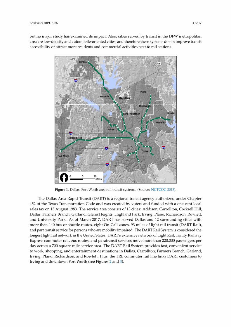
Rail passenger transportation in the Dallas–Fort Worth Metropolitan Area is provided by threeregional transit agencies—including Dallas Area Rapid Transit (DART), Denton County TransportationAuthority (DCTA), and Trinity Railway Express (TRE)—and serves four urban counties (Collin, Dallas,Denton, and Tarrant) as shown in Figure 1, (NCTCOG 2013). Most of the figures in the paper arefrom the North Central Texas Council of Government (NCTCOG), which is the regional council forthis urban region. In these four counties, 20 cities are served by 74 rail stations along 146 miles oflight and commuter rail, as shown in Figure 1. DART is the largest agency that provides rail services.It covers 13-member cities along 90 miles of light rail transit (59 rail stations). TRE as a commuterrail links downtown Fort Worth and downtown Dallas in this twin center combined metropolitanregion with roughly 35 miles of commuter rail service (10 stations) in four cities; DCTA provides21 miles of commuter rail that serves three cities (6 stations) (NCTCOG 2015). As mentioned earlier,one motivating factor for doing this study is that the DFW area has the longest rail transit system,

Economies 2019, 7, 86 4 of 17

but no major study has examined its impact. Also, cities served by transit in the DFW metropolitanarea are low-density and automobile-oriented cities, and therefore these systems do not improve transitaccessibility or attract more residents and commercial activities next to rail stations.

Economies 2019, 7, x FOR PEER REVIEW 4 of 17

do not improve transit accessibility or attract more residents and commercial activities next to rail stations.

Figure 1. Dallas–Fort Worth area rail transit systems. Source: NCTCOG, 2013.

The Dallas Area Rapid Transit (DART) is a regional transit agency authorized under Chapter 452 of the Texas Transportation Code and was created by voters and funded with a one-cent local sales tax on 13 August 1983. The service area consists of 13 cities: Addison, Carrollton, Cockrell Hill, Dallas, Farmers Branch, Garland, Glenn Heights, Highland Park, Irving, Plano, Richardson, Rowlett, and University Park. As of March 2017, DART has served Dallas and 12 surrounding cities with more than 140 bus or shuttle routes, eight On-Call zones, 93 miles of light rail transit (DART Rail), and paratransit service for persons who are mobility impaired. The DART Rail System is considered the longest light rail network in the United States. DART’s extensive network of Light Rail, Trinity Railway Express commuter rail, bus routes, and paratransit services move more than 220,000 passengers per day across a 700-square-mile service area. The DART Rail System provides fast, convenient service to work, shopping, and entertainment destinations in Dallas, Carrollton, Farmers Branch, Garland, Irving, Plano, Richardson, and Rowlett. Plus, the TRE commuter rail line links DART customers to Irving and downtown Fort Worth (see Figures 2 and 3).

Figure 1. Dallas–Fort Worth area rail transit systems. (Source: NCTCOG 2013).

The Dallas Area Rapid Transit (DART) is a regional transit agency authorized under Chapter452 of the Texas Transportation Code and was created by voters and funded with a one-cent localsales tax on 13 August 1983. The service area consists of 13 cities: Addison, Carrollton, Cockrell Hill,Dallas, Farmers Branch, Garland, Glenn Heights, Highland Park, Irving, Plano, Richardson, Rowlett,and University Park. As of March 2017, DART has served Dallas and 12 surrounding cities withmore than 140 bus or shuttle routes, eight On-Call zones, 93 miles of light rail transit (DART Rail),and paratransit service for persons who are mobility impaired. The DART Rail System is considered thelongest light rail network in the United States. DART’s extensive network of Light Rail, Trinity RailwayExpress commuter rail, bus routes, and paratransit services move more than 220,000 passengers perday across a 700-square-mile service area. The DART Rail System provides fast, convenient serviceto work, shopping, and entertainment destinations in Dallas, Carrollton, Farmers Branch, Garland,Irving, Plano, Richardson, and Rowlett. Plus, the TRE commuter rail line links DART customers toIrving and downtown Fort Worth (see Figures 2 and 3).

Economies 2019, 7, 86 5 of 17

Economies 2019, 7, x FOR PEER REVIEW 5 of 17

Figure 2. DART Service Area. Source: DART, 2017.

DART is considered part of the Dallas–Fort Worth Metropolitan (DFW) Area in which congestion levels and road conditions are getting worse. Automobile-dependence is a concern for many reasons, including congestion in urban areas, pollution, and environmental damage caused by pollution. The level of congestion/delay is expected to increase substantially in the DFW area between the year 2017 and 2040 (see Figures 4 and 5).

Switching to more sustainable, environmentally friendly and less congesting transportation modes, such as public transit, is likely to be an effective solution to most of these problems. Moreover, in the DART study area, the population is expected to grow significantly due to the influx of people moving from other States into the DFW area (see Figure 6). The employment level is also expected to increase substantially in the DFW area (see Figure 7). Population and employment increases are expected to have a positive impact on transit ridership.

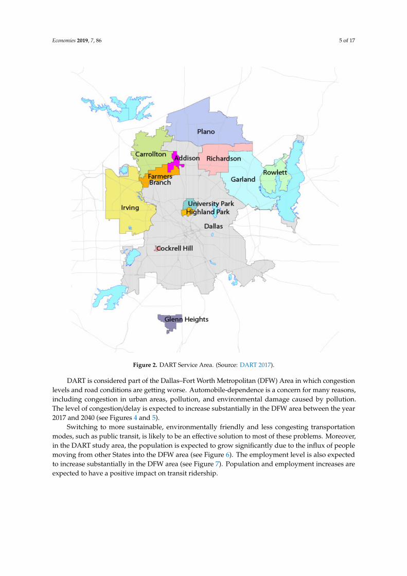
Figure 2. DART Service Area. (Source: DART 2017).

DART is considered part of the Dallas–Fort Worth Metropolitan (DFW) Area in which congestionlevels and road conditions are getting worse. Automobile-dependence is a concern for many reasons,including congestion in urban areas, pollution, and environmental damage caused by pollution.The level of congestion/delay is expected to increase substantially in the DFW area between the year2017 and 2040 (see Figures 4 and 5).

Switching to more sustainable, environmentally friendly and less congesting transportationmodes, such as public transit, is likely to be an effective solution to most of these problems. Moreover,in the DART study area, the population is expected to grow significantly due to the influx of peoplemoving from other States into the DFW area (see Figure 6). The employment level is also expectedto increase substantially in the DFW area (see Figure 7). Population and employment increases areexpected to have a positive impact on transit ridership.

Economies 2019, 7, 86 6 of 17

Economies 2019, 7, x FOR PEER REVIEW 6 of 17

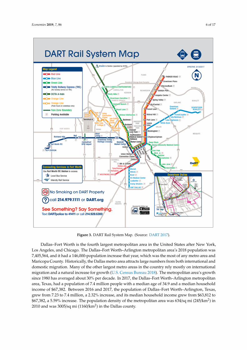
Figure 3. DART Rail System Map. (Source: DART 2017).

Dallas–Fort Worth is the fourth largest metropolitan area in the United States after New York, Los Angeles, and Chicago. The Dallas–Fort Worth–Arlington metropolitan area’s 2018 population was 7,405,564, and it had a 146,000-population increase that year, which was the most of any metro area and Maricopa County. Historically, the Dallas metro area attracts large numbers from both international and domestic migration. Many of the other largest metro areas in the country rely mostly on international migration and a natural increase for growth (U.S. Census 2018). The metropolitan area’s growth since 1980 has averaged about 30% per decade. In 2017, the Dallas–Fort Worth–Arlington metropolitan area, Texas, had a population of 7.4 million people with a median age of 34.9 and a median household income of $67,382. Between 2016 and 2017, the population of Dallas–Fort Worth–Arlington, Texas, grew from 7.23 to 7.4 million, a 2.32% increase, and its median household income grew from $63,812 to $67,382, a 5.59% increase. The population density of the metropolitan area was 634/sq mi (245/km2) in 2010 and was 3005/sq mi (1160/km2) in the Dallas county.

Figure 3. DART Rail System Map. (Source: DART 2017).

Dallas–Fort Worth is the fourth largest metropolitan area in the United States after New York,Los Angeles, and Chicago. The Dallas–Fort Worth–Arlington metropolitan area’s 2018 population was7,405,564, and it had a 146,000-population increase that year, which was the most of any metro area andMaricopa County. Historically, the Dallas metro area attracts large numbers from both international anddomestic migration. Many of the other largest metro areas in the country rely mostly on internationalmigration and a natural increase for growth (U.S. Census Bureau 2018). The metropolitan area’s growthsince 1980 has averaged about 30% per decade. In 2017, the Dallas–Fort Worth–Arlington metropolitanarea, Texas, had a population of 7.4 million people with a median age of 34.9 and a median householdincome of $67,382. Between 2016 and 2017, the population of Dallas–Fort Worth–Arlington, Texas,grew from 7.23 to 7.4 million, a 2.32% increase, and its median household income grew from $63,812 to$67,382, a 5.59% increase. The population density of the metropolitan area was 634/sq mi (245/km2) in2010 and was 3005/sq mi (1160/km2) in the Dallas county.

Economies 2019, 7, 86 7 of 17

Economies 2019, 7, x FOR PEER REVIEW 7 of 17

Figure 4. 2017 Levels of Congestion/ Delay. (Source: NCTCOG 2017).

Figure 5. 2040 Levels of Congestion/Delay. (Source: NCTCOG 2017).

Figure 4. 2017 Levels of Congestion/ Delay. (Source: NCTCOG 2017).

Economies 2019, 7, x FOR PEER REVIEW 7 of 17

Figure 4. 2017 Levels of Congestion/ Delay. (Source: NCTCOG 2017).

Figure 5. 2040 Levels of Congestion/Delay. (Source: NCTCOG 2017). Figure 5. 2040 Levels of Congestion/Delay. (Source: NCTCOG 2017).

Economies 2019, 7, 86 8 of 17

Economies 2019, 7, x FOR PEER REVIEW 8 of 17

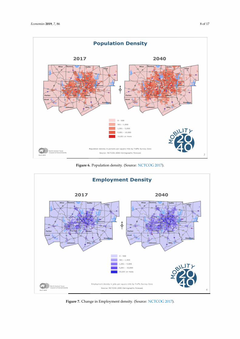
Figure 6. Population density. (Source: NCTCOG 2017).

Figure 7. Change in Employment density. (Source: NCTCOG 2017).

The population of Dallas–Fort Worth–Arlington metropolitan area is 46.3% White Alone, 28.9% Hispanic or Latino, and 15.4% Black or African American Alone. From 2016 to 2017, employment in Dallas–Fort Worth–Arlington, Texas, grew at a rate of 2.75%, from 3.61 to 3.71 million employees.

Figure 6. Population density. (Source: NCTCOG 2017).

Economies 2019, 7, x FOR PEER REVIEW 8 of 17

Figure 6. Population density. (Source: NCTCOG 2017).

Figure 7. Change in Employment density. (Source: NCTCOG 2017).

The population of Dallas–Fort Worth–Arlington metropolitan area is 46.3% White Alone, 28.9% Hispanic or Latino, and 15.4% Black or African American Alone. From 2016 to 2017, employment in Dallas–Fort Worth–Arlington, Texas, grew at a rate of 2.75%, from 3.61 to 3.71 million employees.

Figure 7. Change in Employment density. (Source: NCTCOG 2017).

Economies 2019, 7, 86 9 of 17

The population of Dallas–Fort Worth–Arlington metropolitan area is 46.3% White Alone, 28.9%Hispanic or Latino, and 15.4% Black or African American Alone. From 2016 to 2017, employmentin Dallas–Fort Worth–Arlington, Texas, grew at a rate of 2.75%, from 3.61 to 3.71 million employees.Households have a median annual income of $67,382, which is more than the median annual incomeof $60,336 across the entire United States. Using averages, employees in Dallas–Fort Worth–Arlingtonhave a longer commute time (27 min) than the normal US worker (25.5 min). Additionally, 1.92% ofthe workforce in the region have “super commutes” for more than 90 min. The public transit usehas been merely at the 8% level. In 2017, the most common method of travel for workers in theDallas–Fort Worth–Arlington area was Drove-alone, 80.9%, followed by those who carpooled, 9.61%(Data USA 2018).

4. Intelligent Transit Information Systems (ITIS) Applications Overview

In 2010, Trapeze ITS, a provider of solutions to the public passenger transportation industry,was chosen by DART for its intelligent transit transportation system implementations. DART selectedTrapeze INFO-Web for its online trip-planning software. Buses and trains were equipped withGPS based Automatic Vehicle Location (AVL), automatic passenger counters, and a private radiosystem for operator voice communications to dispatch vehicle location data every 90 s by 4G wireless.This information has helped DART, like many other public transit systems, reach its full potential andaddress concerns about the uncertainty of arrival times and limited connectivity, in addition to safetyand comfort. DART has strived to collect more information about the location of their vehicles andto provide this information to their customers. The availability of global positioning system (GPS)data was a necessary step for addressing the uncertainty concerns, but it was only part of the solutionbecause location information had to be communicated in real-time to the public. ITIS applicationson user-friendly devices such as smartphones, personal digital assistants (PDAs), and desktops canprovide that missing link.

Integration with the existing schedule data was another factor as changes to the schedules wereimmediately reflected on their website, with no need for manual updating or uploading of data.The system is also characterized by its simplicity: Riders enter a starting point, a destination, and apreferred departure or arrival time, and itineraries are generated using scheduling and routing datafrom the scheduling system. Results can be sorted by total trip time, a number of transfers, and walkingdistances. Drop-down menus also allow riders to select landmarks such as shopping centers orhospitals as their origin and destination points. DART has also implemented an application underlyinga new radio communications system which provides a trove of real-time (or close) trip data foroperational metrics and analysis. Using business intelligence tools, this system will be linked to datafrom other modules to deliver management information routinely and on-demand.

Additionally, DART has made strides in delivering information to riders. Using a desktop ormobile browser, riders can receive real-time predicted bus arrival times at a stop. Smartphones canalso be used to locate the nearest DART stop, with a street view, and then show routes at that stop,trip planning, and predicted bus or train arrival times. Text capability has been added, using thebus stop ID and short code to extend the arrival prediction service to riders with regular cell phones.Subscriptions to social media sites and email enable direct messages to riders about incidents on theirchosen routes.

5. Methods and Techniques

To understand the impact of important socioeconomic variables and ITIS on transit ridership inthe Dallas Area Rapid Transit, this study covers the period between 2007–2017. The analysis consideredin this section attempts to explain transit ridership for the combined ridership of rail and bus andstudies several independent variables selected based on the literature. The focus is on transit ridershipto evaluate the effect of factors on its decline or increase. The analysis attempts to understand thevariation of ridership for public transit, considering several independent variables selected based on a

Economies 2019, 7, 86 10 of 17

comprehensive review of the theoretical and empirical literature. The analysis for transit ridership isalso intended to evaluate the impact of the application of ITIS along with other important variables todevelop and explain the monthly transit ridership in DART area in a comprehensive manner with timeseries monthly data for the ten years.

6. Data and Analysis

In this type of research, quite frequently one may be interested in interpreting the effect of a onepercent increase of an independent variable on the dependent variable, which can also be achievedthrough a double-log (log–log) model. This can be transformed by taking the logarithm from both sides.

Log y = logα + β1logx1 + β2logx2 + β3 logx3 + e (1)

where e = log ε.In the full logarithm nonlinear form, the b coefficients will constitute elasticities. Essentially, if we

run the model proposed in this study, the coefficients will constitute the elasticities.

Log Transit Ridership = logα + β1logIncome + β2logITIS + . . . +β24 logFare + e (2)

In order to do the research, the null hypothesis (Ho) is usually constructed to make its rejectionspossible and get the desired result, which is the alternative hypothesis (Ha). However, the alternativehypothesis (Ha: β , 0) is that all independent variables have a statistically significant impact ontransit ridership for the period between 2007 and 2017. Hypotheses have been stated based on theexpected results. So, hypotheses for the research question are as follows. As fare, income, temperature,precipitation, freeze, and snow increase, transit ridership will decrease.

On the other hand, as gas prices, car trips (congestion), unemployment, poverty, and the ITISapplication usage increase, transit ridership will increase. ITIS increases transit ridership because itreduces negative aspects and the cost of using transit through providing information, saving time andother attributes, and makes transit more competitive with the automobile

In this study, the datasets consist of ridership, socio-economic data, and ITIS applications usagedata for the entire DART Area from January of 2007 to present in a monthly base. Given that theintelligent transit information systems applications were implemented in 2012, this enables the studyto capture any seasonal changes over this period or roughly few years before the implementation ofITIS transit applications to a few years after. The required data for this study was obtained from a widevariety of sources. The study uses a time-series perspective to examine changes in transit ridershipover ten years period in a monthly base to capture the incremental exposure to ITIS technology.Most of the socioeconomic data were found in the Census and the American Community Survey(ACS). The changes in these socioeconomic data impacting the transit system in the DFW area help toanswer the research questions. The North Central Texas Council of Governments (NCTCOG) providesobjective data and analysis on the development of the region related to urban planning and economicactivities such as development data, employment estimates, and Geographic Information System (GIS)layers. This source also provides some data related to DART and the study area and all geocodedinformation needed for converting some data from other jurisdictions into the DART operation area.The Dallas Area Rapid Transit (DART) provided the ITIS data.

To explore the effect of a percent increase of an affecting variable on the transit ridership,a double-log model was used. As such, the elasticity of demand for transit with respect to some ofthe factors in the model such as percent change in fare, income, or the research question variable,ITIS usage, are examined. Descriptive statistics for the dependent and independent variables arepresented in Table 1. The mean transit ridership in DART area between 2007 and 2017 was estimatedto be 211,092. The mean rail ridership was 82,225, and the mean bus ridership was 128,866. The ITISapplication usage mean was estimated to be 53,280. The mean Car Trips was 20,959, and the mean percapita income was $44,620. The mean Gas price per gallon was $2.74, and the mean Fare was $1.62.

Economies 2019, 7, 86 11 of 17

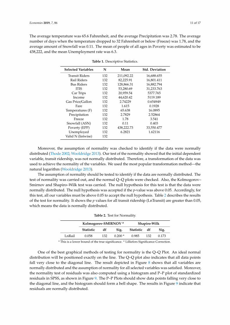
The average temperature was 65.6 Fahrenheit, and the average Precipitation was 2.78. The averagenumber of days when the temperature dropped to 32 Fahrenheit or below (Freeze) was 1.78, and theaverage amount of Snowfall was 0.11. The mean of people of all ages in Poverty was estimated to be438,222, and the mean Unemployment rate was 6.3.

Table 1. Descriptive Statistics.

Selected Variables N Mean Std. Deviation

Transit Riders 132 211,092.22 16,688.655Rail Riders 132 82,225.91 16,801.411Bus Riders 132 128,866.31 16,882.794

ITIS 132 53,280.69 31,233.763Car Trips 132 20,959.54 5377.765Income 132 44,620.42 5119.189

Gas Price/Gallon 132 2.74229 0.654949Fare 132 1.615 0.1928

Temperatures (F) 132 65.638 16.0895Precipitation 132 2.7829 2.52864

Freeze 132 1.78 3.541Snowfall (ASN) 132 0.11 0.403Poverty (EPP) 132 438,222.73 33,550.477Unemployed 132 6.2821 1.62116

Valid N (listwise) 132

Moreover, the assumption of normality was checked to identify if the data were normallydistributed (Thode 2002; Wooldridge 2013). Our test of the normality showed that the initial dependentvariable, transit ridership, was not normally distributed. Therefore, a transformation of the data wasused to achieve the normality of the variables. We used the most popular transformation method—thenatural logarithm (Wooldridge 2013).

The assumption of normality should be tested to identify if the data are normally distributed. Thetest of normality was carried out, and the normal Q–Q plots were checked. Also, the Kolmogorov–Smirnov and Shapiro–Wilk test was carried. The null hypothesis for this test is that the data werenormally distributed. The null hypothesis was accepted if the p-value was above 0.05. Accordingly, forthis test, all our variables must be above 0.05 to accept the null hypothesis. Table 2 describes the resultsof the test for normality. It shows the p values for all transit ridership (LnTransit) are greater than 0.05,which means the data is normally distributed.

Table 2. Test for Normality.

Kolmogorov-SMIRNOV a Shapiro-Wilk

Statistic df Sig. Statistic df Sig.

LnRail 0.058 132 0.200 * 0.985 132 0.173

* This is a lower bound of the true significance. a Lilliefors Significance Correction.

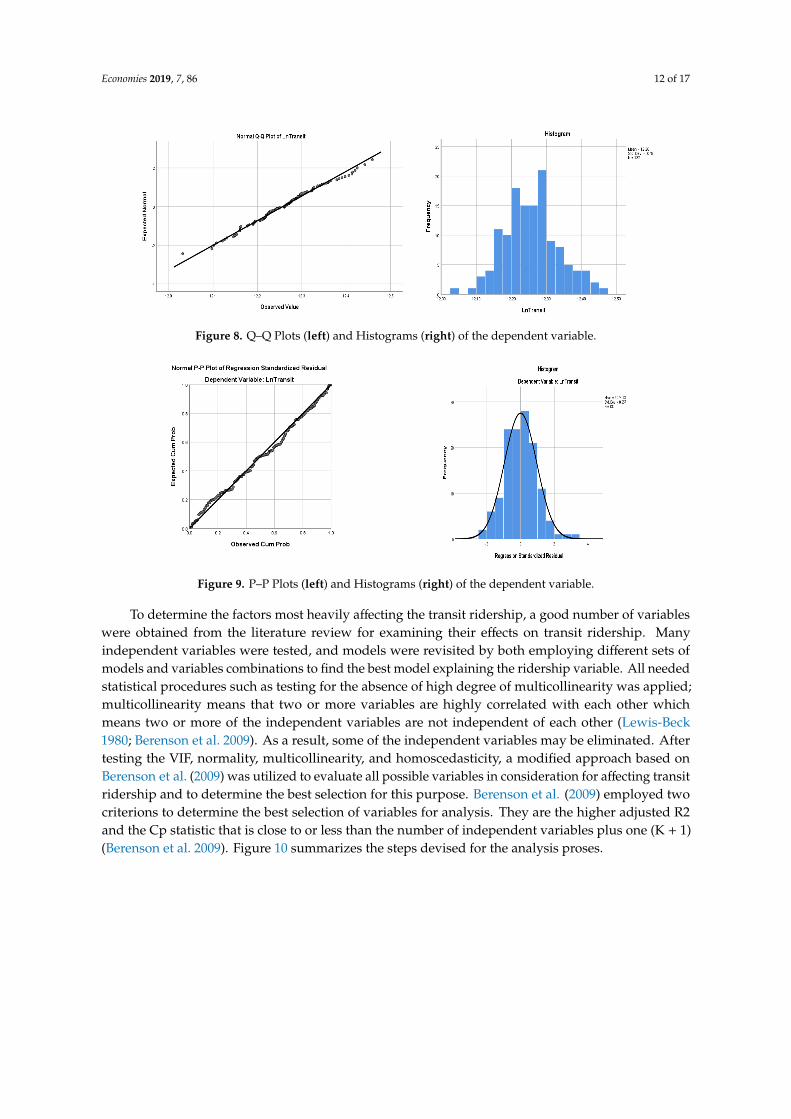
One of the best graphical methods of testing for normality is the Q–Q Plot. An ideal normaldistribution will be positioned exactly on the line. The Q–Q plot also indicates that all data pointsfall very close to the diagonal line. The result depicted in Figure 8 shows that all variables arenormally distributed and the assumption of normality for all selected variables was satisfied. Moreover,the normality test of residuals was also computed using a histogram and P–P plot of standardizedresiduals in SPSS, as shown in Figure 9. The P–P Plots should show data points falling very close tothe diagonal line, and the histogram should form a bell shape. The results in Figure 9 indicate thatresiduals are normally distributed.

Economies 2019, 7, 86 12 of 17Economies 2019, 7, x FOR PEER REVIEW 12 of 17

Figure 8. Q–Q Plots (left) and Histograms (right) of the dependent variable.

Figure 9. P–P Plots (left) and Histograms (right) of the dependent variable.

To determine the factors most heavily affecting the transit ridership, a good number of variables were obtained from the literature review for examining their effects on transit ridership. Many independent variables were tested, and models were revisited by both employing different sets of models and variables combinations to find the best model explaining the ridership variable. All needed statistical procedures such as testing for the absence of high degree of multicollinearity was applied; multicollinearity means that two or more variables are highly correlated with each other which means two or more of the independent variables are not independent of each other (Lewis-Beck 1980; Berenson et al. 2009). As a result, some of the independent variables may be eliminated. After testing the VIF, normality, multicollinearity, and homoscedasticity, a modified approach based on Berenson et al. (2009) was utilized to evaluate all possible variables in consideration for affecting transit ridership and to determine the best selection for this purpose. Berenson et al. (2009) employed two criterions to determine the best selection of variables for analysis. They are the higher adjusted R2 and the Cp statistic that is close to or less than the number of independent variables plus one (K + 1) (Berenson et al. 2009). Figure 10 summarizes the steps devised for the analysis proses.

Figure 8. Q–Q Plots (left) and Histograms (right) of the dependent variable.

Economies 2019, 7, x FOR PEER REVIEW 12 of 17

Figure 8. Q–Q Plots (left) and Histograms (right) of the dependent variable.

Figure 9. P–P Plots (left) and Histograms (right) of the dependent variable.

To determine the factors most heavily affecting the transit ridership, a good number of variables were obtained from the literature review for examining their effects on transit ridership. Many independent variables were tested, and models were revisited by both employing different sets of models and variables combinations to find the best model explaining the ridership variable. All needed statistical procedures such as testing for the absence of high degree of multicollinearity was applied; multicollinearity means that two or more variables are highly correlated with each other which means two or more of the independent variables are not independent of each other (Lewis-Beck 1980; Berenson et al. 2009). As a result, some of the independent variables may be eliminated. After testing the VIF, normality, multicollinearity, and homoscedasticity, a modified approach based on Berenson et al. (2009) was utilized to evaluate all possible variables in consideration for affecting transit ridership and to determine the best selection for this purpose. Berenson et al. (2009) employed two criterions to determine the best selection of variables for analysis. They are the higher adjusted R2 and the Cp statistic that is close to or less than the number of independent variables plus one (K + 1) (Berenson et al. 2009). Figure 10 summarizes the steps devised for the analysis proses.

Figure 9. P–P Plots (left) and Histograms (right) of the dependent variable.

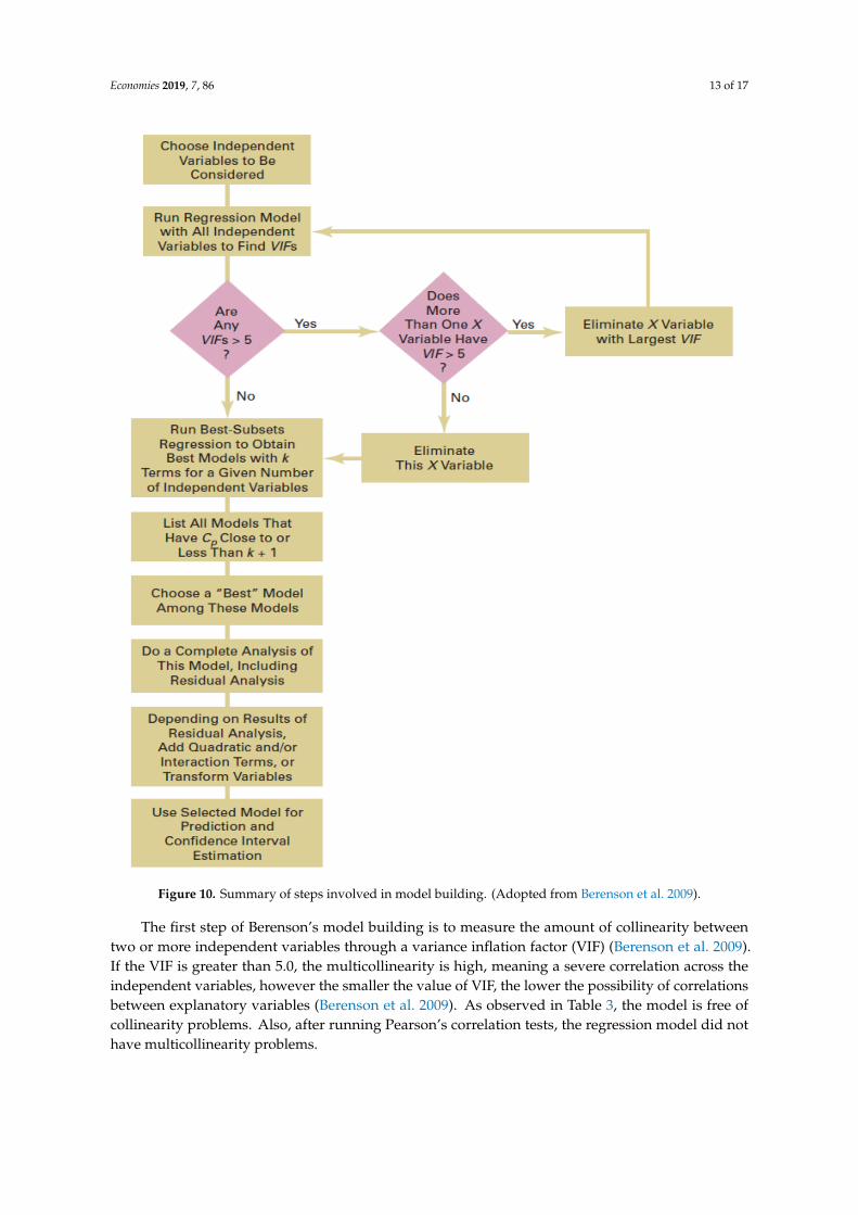
To determine the factors most heavily affecting the transit ridership, a good number of variableswere obtained from the literature review for examining their effects on transit ridership. Manyindependent variables were tested, and models were revisited by both employing different sets ofmodels and variables combinations to find the best model explaining the ridership variable. All neededstatistical procedures such as testing for the absence of high degree of multicollinearity was applied;multicollinearity means that two or more variables are highly correlated with each other whichmeans two or more of the independent variables are not independent of each other (Lewis-Beck1980; Berenson et al. 2009). As a result, some of the independent variables may be eliminated. Aftertesting the VIF, normality, multicollinearity, and homoscedasticity, a modified approach based onBerenson et al. (2009) was utilized to evaluate all possible variables in consideration for affecting transitridership and to determine the best selection for this purpose. Berenson et al. (2009) employed twocriterions to determine the best selection of variables for analysis. They are the higher adjusted R2and the Cp statistic that is close to or less than the number of independent variables plus one (K + 1)(Berenson et al. 2009). Figure 10 summarizes the steps devised for the analysis proses.

Economies 2019, 7, 86 13 of 17Economies 2019, 7, x FOR PEER REVIEW 13 of 17

Figure 10. Summary of steps involved in model building. (Adopted from Berenson et al. 2009).

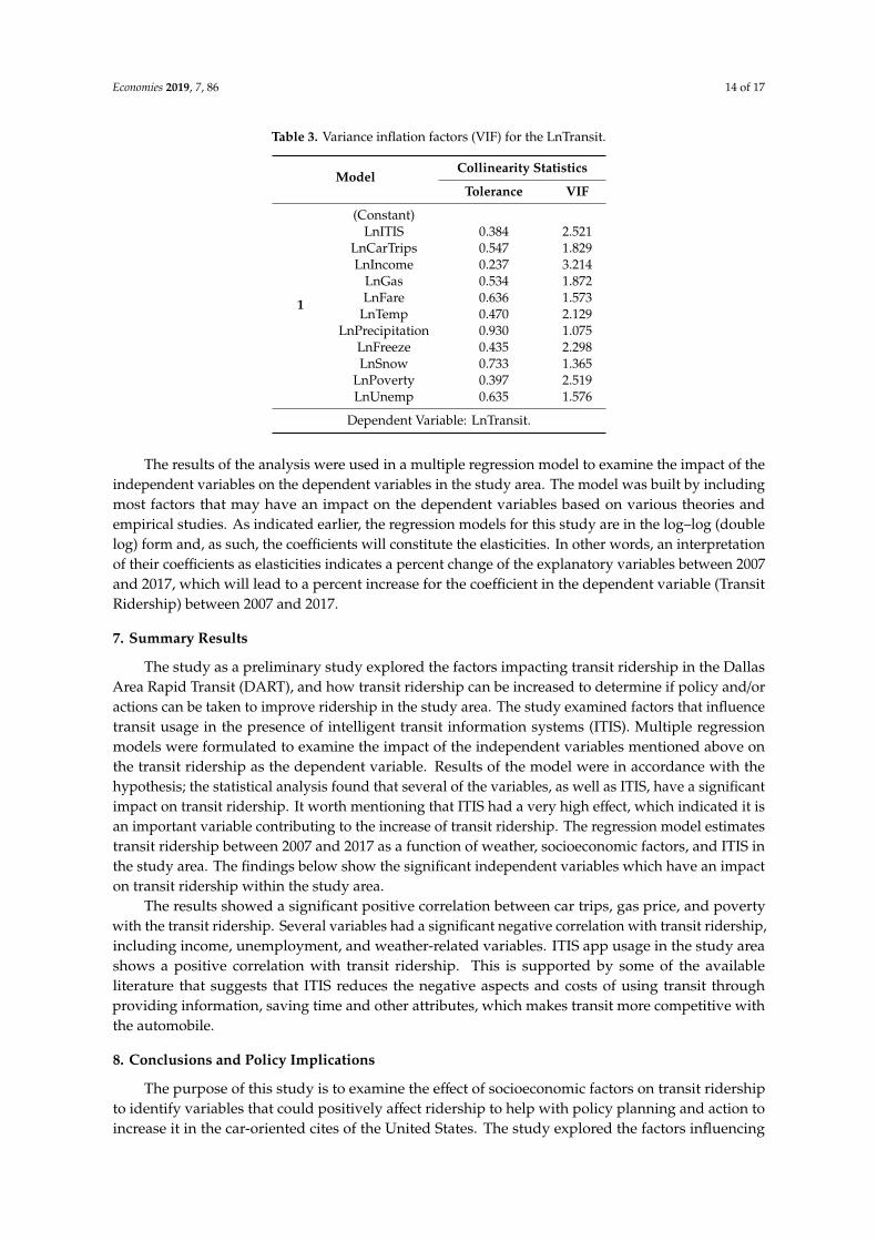
The first step of Berenson’s model building is to measure the amount of collinearity between two or more independent variables through a variance inflation factor (VIF) (Berenson et al. 2009). If the VIF is greater than 5.0, the multicollinearity is high, meaning a severe correlation across the independent variables, however the smaller the value of VIF, the lower the possibility of correlations between explanatory variables (Berenson et al. 2009). As observed in Table 3, the model is free of collinearity problems. Also, after running Pearson’s correlation tests, the regression model did not have multicollinearity problems.

Figure 10. Summary of steps involved in model building. (Adopted from Berenson et al. 2009).

The first step of Berenson’s model building is to measure the amount of collinearity betweentwo or more independent variables through a variance inflation factor (VIF) (Berenson et al. 2009).If the VIF is greater than 5.0, the multicollinearity is high, meaning a severe correlation across theindependent variables, however the smaller the value of VIF, the lower the possibility of correlationsbetween explanatory variables (Berenson et al. 2009). As observed in Table 3, the model is free ofcollinearity problems. Also, after running Pearson’s correlation tests, the regression model did nothave multicollinearity problems.

Economies 2019, 7, 86 14 of 17

Table 3. Variance inflation factors (VIF) for the LnTransit.

ModelCollinearity Statistics

Tolerance VIF

1

(Constant)LnITIS 0.384 2.521

LnCarTrips 0.547 1.829LnIncome 0.237 3.214

LnGas 0.534 1.872LnFare 0.636 1.573

LnTemp 0.470 2.129LnPrecipitation 0.930 1.075

LnFreeze 0.435 2.298LnSnow 0.733 1.365

LnPoverty 0.397 2.519LnUnemp 0.635 1.576

Dependent Variable: LnTransit.

The results of the analysis were used in a multiple regression model to examine the impact of theindependent variables on the dependent variables in the study area. The model was built by includingmost factors that may have an impact on the dependent variables based on various theories andempirical studies. As indicated earlier, the regression models for this study are in the log–log (doublelog) form and, as such, the coefficients will constitute the elasticities. In other words, an interpretationof their coefficients as elasticities indicates a percent change of the explanatory variables between 2007and 2017, which will lead to a percent increase for the coefficient in the dependent variable (TransitRidership) between 2007 and 2017.

7. Summary Results

The study as a preliminary study explored the factors impacting transit ridership in the DallasArea Rapid Transit (DART), and how transit ridership can be increased to determine if policy and/oractions can be taken to improve ridership in the study area. The study examined factors that influencetransit usage in the presence of intelligent transit information systems (ITIS). Multiple regressionmodels were formulated to examine the impact of the independent variables mentioned above onthe transit ridership as the dependent variable. Results of the model were in accordance with thehypothesis; the statistical analysis found that several of the variables, as well as ITIS, have a significantimpact on transit ridership. It worth mentioning that ITIS had a very high effect, which indicated it isan important variable contributing to the increase of transit ridership. The regression model estimatestransit ridership between 2007 and 2017 as a function of weather, socioeconomic factors, and ITIS inthe study area. The findings below show the significant independent variables which have an impacton transit ridership within the study area.

The results showed a significant positive correlation between car trips, gas price, and povertywith the transit ridership. Several variables had a significant negative correlation with transit ridership,including income, unemployment, and weather-related variables. ITIS app usage in the study areashows a positive correlation with transit ridership. This is supported by some of the availableliterature that suggests that ITIS reduces the negative aspects and costs of using transit throughproviding information, saving time and other attributes, which makes transit more competitive withthe automobile.

8. Conclusions and Policy Implications

The purpose of this study is to examine the effect of socioeconomic factors on transit ridershipto identify variables that could positively affect ridership to help with policy planning and action toincrease it in the car-oriented cites of the United States. The study explored the factors influencing

Economies 2019, 7, 86 15 of 17

transit ridership in Dallas Area Rapid Transit (DART) as a case in car-oriented cities, and also examinedthe effect of intelligent transportation information systems (ITIS). The study identified major factorsthrough a comprehensive review of literature, use of an innovative process which assisted the selectionof the most significant variable, and a time series regression mode to study the effects of variables inthe study area between 2007 and 2017 through use of monthly data.

Some of the significant variables through the findings have major policy implications. For example,the study showed that poverty has a positive correlation with transit ridership. This correlation meansthat as poverty increases, ridership increases. This finding suggests that poor individuals are mostlikely to choose public transportation for access to employment and other household necessities in anurban setting like the study area. Since the demand for transit is higher for the low-income populationwho also had to cut from their other living expenses to afford transportation, it behooves that transitshould be subsidized for the low-income population. This is also supported by the findings that,as expected, fare price has a negative correlation with ridership and was statistically significant, whichconforms to existing literature and suggests that as fare increases, ridership decreases within the studyarea. It also is in line with findings that income has a negative correlation with transit ridership.As income increases, bus ridership decreases. This finding suggests that low-income individuals aremost likely to rely on public transportations for access to employment and other household necessities,a further justification for the subsidy.

Finally, the ITIS app usage in the study area shows a positive correlation with transit ridership;as the ITIS app usage increases, transit ridership also increases. This is supported by some of theavailable literature that suggests that ITIS reduces the negative aspects and costs of using transitthrough providing information, saving time, and other attributes, that makes transit more competitivewith the automobile. The results showed that ITIS has been affecting transit ridership, and it showedthat ITIS contributed to a significant increase in transit ridership; as people got to know aboutthe availability of the service and used it more, the ridership increased. The implication is thattransit organizations investments in intelligent transportation information systems and furthering itscapabilities is warranted and should be encouraged. It reduces the negative aspects of using transitfor consumers.

As was mentioned, this study was a preliminary exploration of the determinants of transitridership, and further study need to overcome the limitations of this study. Future research needs tofurther detail the ridership study and improve the findings. More importantly, the breakdown of theridership by transit modes could shed light on the effect of important identified factors on differenttransit modes.

Author Contributions: This article is part of a larger and an ongoing research that become A.D.’s dissertationwith A.A. as the dissertation supervising professor. A.D. has undertaken the initial research and analysis workunder A.A.’s guidance, and A.A. has drafted and prepared the article for the publication.

Funding: This research received no external funding.

Acknowledgments: The authors would like to acknowledge the generous support of the Dallas Area RapidTransit (DART) by providing the ITIS and other data that has made this research possible.

Conflicts of Interest: The authors declare no conflict of interest.

References

Alam, Bhuian M. 2009. Transit Accessibility to Jobs and Employment Prospects of Welfare Recipients WithoutCars. Transportation Research Record: Journal of the Transportation Research Board 2110: 78–86. [CrossRef]

Alam, Bhuiyan M., Hilary Nixon, and Qiong Zhang. 2015. Investigating the Determining Factors for TransitTravel Demand by Bus Mode in US Metropolitan Statistical Areas. Transportation Research Record: Journal ofthe Transportation Research Board 2110: 78–86. [CrossRef]

Armbruster, Brendan. 2010. Factors Affecting Transit Ridership at the Metropolitan Level 2002–2007.Master’s Thesis, Georgetown University, Washington, DC, USA.

Economies 2019, 7, 86 16 of 17

Berenson, Mark, David Levine, and Timothy Krehbiel. 2009. Basic Business Statistics: Concepts and Applications,12th ed. Upper Saddle River: Prentice-Hall.

Boarnet, Marlone G., and Randall Crane. 2001. Travel by Design: The Influence of Urban Form on Travel. Oxford andNew York: Oxford University Press.

Borghesi, Simone, Chiara Calastri, and Giorgio Fagiolo. 2014. How Do People Choose Their Commuting Mode?An Evolutionary Approach to Transport Choices. LEM Papers Series; Pisa: Laboratory of Economics andManagement (LEM), Sant’Anna School of Advanced Studies.

Chen, Cynthia, Don Varley, and Jason Chen. 2011. What Affects Transit Ridership? A Dynamic Analysis InvolvingMultiple Factors, Lags and Asymmetric Behaviour. Urban Studies 48: 1893–908. [CrossRef]

Chiang, Wen-Chyuan, Robert A. Russell, and Timothy L. Urban. 2011. Forecasting Ridership for a MetropolitanTransit Authority. Transportation Research Part A: Policy and Practice 45: 696–705. [CrossRef]

Dallas Area Rapid Transit (DART). 2017. DART Reference Book. Dallas: DART, March.Data USA. 2018. Available online: https://datausa.io/profile/geo/dallas-fort-worth-arlington-tx-metro-area

(accessed on 31 July 2019).EIA. 2018. Energy Use for Transportation. Use of Energy in the United States Explained. Available online:

https://www.eia.gov/energyexplained/?page=us_energy_transportation (accessed on 31 July 2019).Fast Facts. 2019. Fast Facts: U.S. Transportation Sector Greenhouse Gas Emissions. 1990–2017. EPA-420-F-19-047.

June. Available online: https://nepis.epa.gov/Exe/ZyPDF.cgi?Dockey=P100WUHR.pdf (accessed on 31 July2019).

Gosselin, Kadley. 2011. Deprivation Study Finds Access to Real-Time Mobile Information Could Raise the Statusof Public Transit. Latitude. Available online: https://latd.com/blog/deprivation-study-finds-access-real-time-mobile-information-raise-status-public-transit/ (accessed on 23 August 2019).

Hickey, Robert L. 2005. Impact of Transit Fare Increase on Ridership and Revenue: Metropolitan TransportationAuthority, New York City. Transportation Research Record: Journal of the Transportation Research Board 1927:239–48. [CrossRef]

Holtzclaw, John, Robert Clear, Hank Dittmar, David Goldstein, and Peter Haas. 2010. Location Efficiency:Neighborhood and Socio-Economic Characteristics Determine Auto Ownership and Use-Studies in Chicago,Los Angeles and San Francisco. Transportation Planning and Technology 25: 1–27. [CrossRef]

Kuby, Michael, Anthony Barranda, and Christopher Upchurch. 2004. Factors Influencing Light-Rail StationBoardings in the United States. Transportation Research Part A: Policy and Practice 38: 223–47. [CrossRef]

Lane, Bradley W. 2010. The Relationship between Recent Gasoline Price Fluctuations and Transit Ridership inMajor US Cities. Journal of Transport Geography 18: 214–25. [CrossRef]

Lane, Bradley W. 2012. A Time-series Analysis of Gasoline Prices and Public Transportation in US MetropolitanAreas. Journal of Transport Geography 22: 221–35. [CrossRef]

Lewis-Beck, Michael S. 1980. Applied Regression: An Introduction. Newbury Park: SAGE.North Central Texas Council of Governments [NCTCOG]. 2013. Congestion Management Process. Available

online: http://www.nctcog.org/trans/cmp/documents/SECT2_SystemID.pdf (accessed on 31 July 2019).North Central Texas Council of Governments [NCTCOG]. 2015. TOD Data Collection. Available online:

http://www.nctcog.org/trans/sustdev/TOD/TODdatacollection.asp (accessed on 31 July 2019).North Central Texas Council of Governments [NCTCOG]. 2017. Mobility 2040 Presentation. Available online:

http://www.nctcog.org/trans/mtp/2040/documents/MapPackage.pdf (accessed on 31 July 2019).Polzin, Steven E., Xuehao Chu, and Joel R. Rey. 2000. Density and Captivity in Public Transit Success: Observations

from the 1995 Nationwide Personal Transportation Study. Transportation Research Record: Journal of theTransportation Research Board 1735: 10–18. [CrossRef]

Pucher, John. 2002. Renaissance of Public Transport in the United States? Transportation Quarterly 56: 33–49.Pucher, John, and John L. Renne. 2003. Socioeconomics of Urban Travel: Evidence from the 2001 NHTS.

Transportation Quarterly 57: 49–77.Renne, John. L. 2009. From Transit-adjacent to Transit-oriented Development. Local Environment 14: 1–15.

[CrossRef]Taylor, Brian D., Douglas Miller, Hiroyuki Iseki, and Camille Fink. 2009. Nature and/or Nurture? Analyzing the

Determinants of Transit Ridership across US Urbanized Areas. Transportation Research Part A: Policy andPractice 43: 60–77. [CrossRef]

Economies 2019, 7, 86 17 of 17

Thode, Henry C., Jr. 2002. Statistics: Textbooks and Monographs, Vol. 164. Testing for Normality. New York:Marcel Dekker.

U.S. Census Bureau. 2018. New Census Bureau Population Estimates Show Dallas-Fort Worth-Arlington HasLargest Growth in the United States. Available online: https://www.census.gov/newsroom/press-releases/2018/popest-metro-county.html (accessed on 31 July 2019).

Wallace, Nick. 2017. The Best Cities for Public Transpiration. Seattle: University of Washington.Weigel, Brent A., Frank Southworth, and Michael D. Meyer. 2010. Calculators for estimating greenhouse gas

emissions from public transit agency vehicle fleet operations. Transportation Research Record 2143: 125–33.Wooldridge, Jeffery M. 2013. Introductory Econometrics: A Modern Approach, 5th ed. Mason: South-Western Cengage

Learning.Zhou, Jiangping, and Lisa Schweitzer. 2011. Getting Drivers to Switch: Transit Price and Service Quality among

Commuters. Journal of Urban Planning and Development 137: 477–83. [CrossRef]

© 2019 by the authors. Licensee MDPI, Basel, Switzerland. This article is an open accessarticle distributed under the terms and conditions of the Creative Commons Attribution(CC BY) license (http://creativecommons.org/licenses/by/4.0/).