publiic finance and public policy - humboldt state...

Jonathan GruberMassachusetts Institute of Technology

Worth Publishers

Public Finance and Public Policy

THIRD EDITION

To Andrea, Sam, Jack, and Ava

Senior Publisher: Craig Bleyer

Senior Acquisitions Editor: Sarah Dorger

Development Editor: Jane Tufts

Media Development Editor: Marie McHale

Senior Marketing Manager: Scott Guile

Assistant Supplements Editor: Tom Acox

Associate Managing Editor: Tracey Kuehn

Project Editor: Leo Kelly, Macmillan Publishing Solutions

Production Manager: Barbara Anne Seixas

Art Director: Babs Reingold

Cover Design: Kevin Kall

Interior Design: Lissi Sigillo

Photo Editor: Cecilia Varas

Composition: MPS Limited, A Macmillan Company

Printing and Binding: RR Donnelley

Cover Photographs: Capitol Building: Photodisc; Image of “Sign Here” Sign on Tax Form: © DavidArky/Corbis; Image of man guiding steel truss: © Rich LaSalle/Getty Images; Image of businessmanholding “Need Work! Work for Food!” Sign: © Michael N. Paras/Corbis; Image of surgery: © DarrenKemper/Corbis; Image of elderly people practicing tai chi: © Peter Mumford/Alamy

ISBN-13: 978-1-4292-1949-5

ISBN-10: 1-4292-1949-1

Library of Congress Control Number: 2006937926

© 2011, 2007, 2005 Worth Publishers

All rights reserved

Printed in the United States of America

First printing, 2010

Worth Publishers

41 Madison Avenue

New York, NY 10010

www.worthpublishers.com

www.worthpublishers.com

2.2 Putting the Tools to Work: TANF and Labor Supply Among Single Mothers . . . . . . . . . . . . . . . . . . . . . . . 37

Identifying the Budget Constraint 38The Effect of TANF on the Budget Constraint 39

2.3 Equilibrium and Social Welfare . . . . . . . . . . . . . . . . . . . 43Demand Curves 44Supply Curves 46Equilibrium 48Social Efficiency 49Competitive Equilibrium Maximizes Social Efficiency 50From Social Efficiency to Social Welfare: The Role of Equity 52Choosing an Equity Criterion 54

2.4 Welfare Implications of Benefit Reductions: The TANF Example Continued . . . . . . . . . . . . . . . . . . . . . . . 55

2.5 Conclusion . . . . . . . . . . . . . . . . . . . . . . . . . . . . . . . 57

Highlights . . . . . . . . . . . . . . . . . . . . . . . . . . . . . . . . . . 57

Questions and Problems . . . . . . . . . . . . . . . . . . . . . . . . . . 58

Advanced Questions . . . . . . . . . . . . . . . . . . . . . . . . . . . . . 59

APPENDIX TO CHAPTER 2 The Mathematics of Utility Maximization . . 60

CHAPTER 3 Empirical Tools of Public Finance . . . . . . . . . . . 63

3.1 The Important Distinction Between Correlation and Causality . . . . . . . . . . . . . . . . . . . . . . . . . 64

The Problem 65

3.2 Measuring Causation with Data We’d Like to Have: Randomized Trials . . . . . . . . . . . . . . . . . . . . . . . . . . . . . . 66

Randomized Trials as a Solution 67The Problem of Bias 67Randomized Trials of ERT 69Randomized Trials in the TANF Context 69Why We Need to Go Beyond Randomized Trials 70

3.3 Estimating Causation with Data We Actually Get: Observational Data . . . . . . . . . . . . . . . . . . . . . . . . . . . . . 71

Time Series Analysis 72Cross -Sectional Regression Analysis 75Quasi-Experiments 80Structural Modeling 83

viii

3.4 Conclusion . . . . . . . . . . . . . . . . . . . . . . . . . . . . . . . 85

Highlights . . . . . . . . . . . . . . . . . . . . . . . . . . . . . . . . . . 85


Advanced Questions . . . . . . . . . . . . . . . . . . . . . . . . . . . . . 86

APPENDIX TO CHAPTER 3 Cross-Sectional Regression Analysis . . . . . 88

CHAPTER 4 Budget Analysis and Deficit Financing . . . . . . . . 91

4.1 Government Budgeting . . . . . . . . . . . . . . . . . . . . . . . . 93The Budget Deficit in Recent Years 93The Budget Process 94

Application: Efforts to Control the Deficit 95Budget Policies and Deficits at the State Level 97

4.2 Measuring the Budgetary Position of the Government: Alternative Approaches . . . . . . . . . . . . . . . . . . . . . . . . . . . 98

Real vs. Nominal 98The Standardized Deficit 99Cash vs. Capital Accounting 100Static vs. Dynamic Scoring 102

4.3 Do Current Debts and Deficits Mean Anything? A Long-Run Perspective . . . . . . . . . . . . . . . . . . . . . . . . . . 103

Background: Present Discounted Value 103Why Current Labels May Be Meaningless 104Alternative Measures of Long -Run Government Budgets 105What Does the U.S. Government Do? 109

Application: The Financial Shenanigans of 2001 112

4.4 Why Do We Care About the Government’s Fiscal Position? . . . . . . . . . . . . . . . . . . . . . . . . . . . . . . 113

Short -Run vs. Long -Run Effects of the Government on the Macroeconomy 113Background: Savings and Economic Growth 114The Federal Budget, Interest Rates, and Economic Growth 115Intergenerational Equity 117

4.5 Conclusion . . . . . . . . . . . . . . . . . . . . . . . . . . . . . . 118

Highlights . . . . . . . . . . . . . . . . . . . . . . . . . . . . . . . . . . 119


Advanced Questions . . . . . . . . . . . . . . . . . . . . . . . . . . . . 120

ix

Once again, we return to your days as an employee of your state’sDepartment of Health and Human Services. After doing the carefultheoretical analysis outlined in the previous section, you are some-

what closer to making a meaningful contribution to the debate between thegovernor and the secretary of Health and Human Services. You can tell thegovernor and the secretary that a reduction in TANF benefits is likely, but notcertain, to raise labor supply among single mothers, and that the implicationsof this response depend on their concerns about equity versus efficiency. Yetthese politicians don’t just want to know that TANF reductions might raiselabor supply, nor are they interested in the graphical calculations of the socialwelfare effects of lower benefits. What they want is numbers.

To provide these numbers, you now turn to the tools of empirical publicfinance, the use of data and statistical methodologies to measure the impactof government policy on individuals and markets. Many of these tools weredeveloped more recently than the classical analyses of utility maximization andmarket equilibrium that we worked with in the last chapter. As a result, theyare also more imperfect, and there are lively debates about the best way toapproach problems like estimating the labor -supply response of single mothersto TANF benefit changes.

In this chapter, we review these empirical methods. In doing so, we encounterthe fundamental issue faced by those doing empirical work in economics: disen-tangling causality from correlation. We say that two economic variables are cor-related if they move together. But this relationship is causal only if one of thevariables is causing the movement in the other. If, instead, there is a third factorthat causes both to move together, the correlation is not causal.

This chapter begins with a review of this fundamental problem. We thenturn to a discussion of the “gold standard” for measuring the causal effectof an intervention (randomized trials) where individuals are randomly assignedto receive or not receive that intervention. While such randomized trialsare much more common in medicine than in public finance, they provide abenchmark against which other empirical methods can be evaluated. We

Empirical Tools of PublicFinance

3

63

3.1 The Important DistinctionBetween Correlation andCausality

3.2 Measuring Causation withData We’d Like to Have:Randomized Trials

3.3 Estimating Causation withData We Actually Get:Observational Data

3.4 Conclusion

Appendix to Chapter 3Cross -Sectional RegressionAnalysis

empirical public finance Theuse of data and statistical meth-ods to measure the impact ofgovernment policy on individu-als and markets.

correlated Two economicvariables are correlated if theymove together.

causal Two economic variablesare causally related if the move-ment of one causes movementof the other.

then discuss the range of other empirical methods used by public financeeconomists to answer questions such as the causal impact of TANF benefitchanges on the labor supply of single mothers. Throughout, we use this TANFexample, using real -world data on benefit levels and the single -mother laborsupply to assess the questions raised by the theoretical analysis of the previouschapter.

3.1The Important Distinction Between Correlationand Causality

There was once a cholera epidemic in Russia. The government, in an effortto stem the disease, sent doctors to the worst -affected areas. The peasants

of a particular province observed a very high correlation between the numberof doctors in a given area and the incidence of cholera in that area. Relying onthis fact, they banded together and murdered their doctors.1

The fundamental problem in this example is that the peasants in thistown clearly confused correlation with causality. They correctly observed thatthere was a positive association between physician presence and the inci-dence of illness. But they took that as evidence that the presence of physi-cians caused illness to be more prevalent. What they missed, of course, wasthat the link actually ran the other way: it was a higher incidence of illness

that caused there to be more physicians present. Instatistics, this is called the identification problem: giventhat two series are correlated, how do you identifywhether one series is causing another?

This problem has plagued not only Russian peas-ants. In 1988, a Harvard University dean conducted aseries of interviews with Harvard freshmen andfound that those who had taken SAT preparationcourses (a much less widespread phenomenon in1988 than today) scored on average 63 points lower(out of 1,600 points) than those who hadn’t. Thedean concluded that SAT preparation courses wereunhelpful and that “the coaching industry is playingon parental anxiety.”2 This conclusion is anotherexcellent example of confusing correlation with cau-sation. Who was most likely to take SAT preparationcourses? Those students who needed the most helpwith the exam! So all this study found was that stu -dents who needed the most help with the SAT

64 P A R T I ■ I N T R O D U C T I O N A N D B A C K G R O U N D

“That’s the gist of what I want to say. Now get me some statistics to base it on”

© T

he N

ew Y

orke

r. Al

l Rig

hts

Rese

rved

.

1 This example is reproduced from Fisher (1976).2 New York Times (1988).

did the worst on the exam. The courses did not cause students to do worse onthe SATs; rather, students who would naturally do worse on the SATs werethe ones who took the courses.

Another example comes from the medical evaluation of the benefits ofbreast -feeding infants. Child -feeding recommendations typically include breast -feeding beyond 12 months, but some medical researchers have documentedincreased rates of malnutrition in breast -fed toddlers. This has led them toconclude that breast -feeding for too long is nutritionally detrimental. But themisleading nature of this conclusion was illustrated by a study of toddlers inPeru that showed that it was those babies who were already underweight ormalnourished who were breast -fed the longest.3 Increased breast -feeding didnot lead to poor growth; children’s poor growth and health led to increasedbreast -feeding.

The ProblemIn all of the foregoing examples, the analysis suffered from a common problem:the attempt to interpret a correlation as a causal relationship without sufficientthought to the underlying process generating the data. Noting that those whotake SAT preparation courses do worse on SATs, or that those infants whobreast -feed longest are the least healthy, is only the first stage in the researchprocess, that of documenting the correlation. Once one has the data on anytwo measures, it is easy to see if they move together, or covary, or if they donot.

What is harder to assess is whether the movements in one measure are caus-ing the movements in the other. For any correlation between two variables Aand B, there are three possible explanations, one or more of which could resultin the correlation:

� A is causing B.� B is causing A.� Some third factor is causing both.

Consider the previous SAT preparation example. The fact is that, for thissample of Harvard students, those who took an SAT prep course performedworse on their SATs. The interpretation drawn by the Harvard administratorwas one of only many possible interpretations:

� SAT prep courses worsen preparation for SATs.� Those who are of lower test -taking ability take preparation courses to

try to catch up.� Those who are generally nervous people like to take prep courses, and

being nervous is associated with doing worse on standardized exams.

The Harvard administrator drew the first conclusion, but the others may beequally valid. Together, these three interpretations show that one cannot interpret

C H A P T E R 3 ■ E M P I R I C A L T O O L S O F P U B L I C F I N A N C E 65

3 Marquis et al. (1997).

this correlation as a causal effect of test preparation on test scores withoutmore information or additional assumptions.

Similarly, consider the breast -feeding interpretation. Once again, there aremany possible interpretations:

� Longer breast -feeding is bad for health.� Those infants who are in the worst health get breast -fed the longest.� The lowest -income mothers breast -feed longer, since this is the cheap-

est form of nutrition for children, and low income is associated withpoor infant health.

Once again, all of these explanations are consistent with the observed cor-relation. But, once again, the studies that argued for the negative effect ofbreast -feeding on health assumed the first interpretation while ignoring theothers.

The general problem that empirical economists face in trying to use exist-ing data to assess the causal influence of one factor on another is that one can-not immediately go from correlation to causation. This is a problem becausefor policy purposes what matters is causation. Policy makers typically want touse the results of empirical studies as a basis for predicting how governmentinterventions will affect behaviors. Knowing that two factors are correlatedprovides no predictive power; prediction requires understanding the causallinks between the factors. For example, the government shouldn’t make policybased on the fact that breast -feeding infants are less healthy. Rather, it shouldassess the true causal effect of breast -feeding on infant health, and use that asa basis for making government policy. The next section begins to explore theanswer to one of the most important questions in empirical research: Howcan one draw causal conclusions about the relationships between correlatedvariables?

3.2Measuring Causation with Data We’d Like to Have:Randomized Trials

One of the most important empirical issues facing society today is under-standing how new medical treatments affect the health of medical

patients. An excellent example of this issue is the case of estrogen replacementtherapy (ERT), a popular treatment for middle -aged and elderly women whohave gone through menopause (the end of menstruation).4 Menopause isassociated with many negative side effects, such as rapid changes in body tem-perature (“hot flashes”), difficulty sleeping, and higher risk of urinary tractinfection. ERT reduces those side effects by mimicking the estrogen producedby the woman’s body before the onset of menopause.


4 For an overview of ERT issues, see Kolata (2002).

There was no question that ERT helped ameliorate the negative sideeffects of menopause, but there was also a concern about ERT. Anecdotal evi-dence suggested that ERT might raise the risk of heart disease, and, in turn,the risk of heart attacks or strokes. A series of studies beginning in the early 1980sinvestigated this issue by comparing women who did and did not receiveERT after menopause. These studies concluded that those who received ERTwere at no higher risk of heart disease than those who did not; indeed, therewas some suggestion that ERT actually lowered heart disease.

There was reason to be concerned, however, that such a comparison didnot truly reflect the causal impact of ERT on heart disease. This is becausewomen who underwent ERT were more likely to be under a doctor’s care, tolead a healthier lifestyle, and to have higher incomes, all of which are associatedwith a lower chance of heart disease (the third channel previously discussed,where some third factor is correlated with both ERT and heart disease). So itis possible that ERT might have raised the risk of heart disease but that thisincrease was masked because the women taking the drug were in better healthotherwise.

Randomized Trials as a SolutionHow can researchers address this problem? The best solution is through the goldstandard of testing for causality: randomized trials. Randomized trials involvetaking a group of volunteers and randomly assigning them to either a treatmentgroup, which gets the medical treatment, or a control group, which does not.Effectively, volunteers are assigned to treatment or control by the flip of a coin.

To see why randomized trials solve our problem, consider what researcherswould ideally do in this context: take one set of older women, replicate them,and place the originals and the clones in parallel universes. Everything wouldbe the same in these parallel universes except for the use of ERT. Then, onecould simply observe the differences in the incidence of heart disease betweenthese two groups of women. Because the women would be precisely the same,we would know by definition that any differences would be causal. That is,there would be only one possible reason why the set of women assigned ERTwould have higher rates of heart disease, since otherwise both sets of womenare the same.

Unfortunately, we live in the real world and not in some science -fiction story,so we can’t do this parallel universe experiment. But, amazingly, we can approx-imate this alternative reality through the randomized trial. This is because of thedefinition of randomization: assignment to treatment groups and control groupsis not determined by anything about the subjects, but by the flip of a coin. As aresult, the treatment group is identical to the control group in every facet butone: the treatment group gets the treatment (in this case, the ERT).

The Problem of BiasWe can rephrase all of the studies we have discussed so far in this chapter inthe treatment/control framework. In the SAT example, the people who took


randomized trial The idealtype of experiment designed totest causality, whereby a groupof individuals is randomly divid-ed into a treatment group,which receives the treatment ofinterest, and a control group,which does not.

treatment group The set ofindividuals who are subject toan intervention being studied.

control group The set of indi-viduals comparable to the treat-ment group who are not subjectto the intervention beingstudied.

Q

preparatory classes were the treatment group and the people who did not takethe classes were the control group. In the breast -feeding example, the infantswho breast -fed for more than a year were the treatment group and the infantswho did not were the control group. In the ERT studies that occurred beforerandomized trials, those who received ERT were the treatment group andthose who did not were the control group. Even in the Russian doctor exam-ple, the areas where the doctors were sent were the treatment group and theareas where the doctors were not sent was the control group. Virtually anyempirical problem we discuss in this course can be thought of as a comparisonbetween treatment and control groups.

We can therefore always start our analysis of an empirical methodologywith a simple question: Do the treatment and control groups differ for anyreason other than the treatment? All of the earlier examples involve cases inwhich the treatment groups differ in consistent ways from those in the controlgroups: those taking SAT prep courses may be of lower test -taking abilitythan those not taking the courses; those breast -fed longest may be in worsehealth than those not breast -fed as long; those taking ERT may be in betterhealth than those not taking ERT. These non -treatment -related differencesbetween treatment and control groups are the fundamental problem in assign-ing causal interpretations to correlations.

We call these differences bias, a term that represents any source of differ-ence between treatment and control groups that is correlated with the treatmentbut is not due to the treatment. The estimates of the impact of SAT prep courseson SAT scores, for example, are biased by the fact that those who take the prepcourses are likely to do worse on the SATs for other reasons. Similarly, the esti-mates of the impact of breast -feeding past one year on health are biased by thefact that those infants in the worst health are the ones likely to be breast -fedthe longest. The estimates of the impact of ERT on heart disease are biased by thefact that those who take ERT are likely in better health than those who do not.Whenever treatment and control groups consistently differ in a manner that iscorrelated with, but not due to, the treatment, there can be bias.

By definition, such differences do not exist in a randomized trial, since thegroups do not differ in any consistent fashion, but rather only by the flip of acoin. Thus, randomized treatment and control groups cannot have consistentdifferences that are correlated with treatment, since there are no consistentdifferences across the groups other than the treatment. As a result, randomizedtrials have no bias, and it is for this reason that randomized trials are the goldstandard for empirically estimating causal effects.

Quick Hint The description of randomized trials here relies on those trials

having fairly large numbers of treatments and controls (large sample sizes). Hav-

ing large sample sizes allows researchers to eliminate any consistent differences

between the groups by relying on the statistical principle called the law of large

numbers: the odds of getting the wrong answer approaches zero as the sample

size grows.


bias Any source of differencebetween treatment and controlgroups that is correlated withthe treatment but is not due tothe treatment.

Suppose that a friend says that he can flip a (fair, not weighted!) coin so that

it always comes up heads. This is not possible; every time a coin is flipped, there

is a 50% chance that it will land tails up. So you give him a quarter and ask him

to prove it. If he flips just once, there is a 50% chance he will get heads and claim

victory. If he flips twice, there is still a 25% chance that he will get heads both

times, and continue to be able to claim victory; that is, there is still the possibil-

ity of getting a biased answer by chance when there is a very small sample.

As he flips more and more times, however, the odds that the coin will come

up heads every time gets smaller and smaller. After just 10 flips, there is only a 1

in 1,024 chance that he will get all heads. After 20 flips, the odds are 1 in

1,048,576. That is, the higher the number of flips, the lower the odds that we

get a biased answer. Likewise, if randomly assigned groups of individuals are

large enough, we can rule out the possibility of bias arising by chance.

Randomized Trials of ERTWhen the National Institutes of Health appointed its first female director, Dr. Bernadine Healy, in 1991, one of her priorities was to sponsor a random-ized trial of ERTs. This randomized trial tracked over 16,000 women ages 50–79 who were recruited to participate in the trial by 40 clinical centers inthe United States. The study was supposed to last 8.5 years but was stoppedafter 5.2 years because its conclusion was already clear: ERT did in fact raisethe risk of heart disease. In particular, women taking ERT were observed toannually have (per 10,000 women): 7 more coronary heart diseases (both fataland nonfatal), 8 more strokes, and 8 more pulmonary embolisms (blood clotsin the lungs). In addition, the study found that women taking ERT had 8more invasive breast cancers as well. Thus, the randomized trial revealed thatthe earlier ERT studies were biased by differences between these groups. Thesenew findings led some doctors to question their decisions to recommendERTs for postmenopausal women.5

Randomized Trials in the TANF ContextMeasuring the health impacts of new medicines is not the only place whererandomized trials are useful; they can be equally useful in the context of pub-lic policy. Suppose that we want to measure the causal impact of TANF onlabor supply. To begin, we gather a large (e.g., 5,000-person) group of singlemothers who are now receiving a $5,000 benefit guarantee. One by one, wetake each single mother into a separate room and flip a coin. If it is heads, theycontinue to receive a benefit guarantee of $5,000; these mothers are the controlgroup whose benefits do not change. If it is tails, then the guarantee is cut to


5 Results of the study are reported in Writing Group for the Women’s Health Initiative Investigators(2002).

$3,000; these mothers are the treatment group who receive the experimentalreduction in their benefits. After we have assigned a guarantee to all of thesemothers, we follow them for a period of time and observe their labor -supplydifferences. Any labor -supply differences would have to be caused by thechange in benefit guarantee, since nothing else differs in a consistent wayacross these groups.

There is a real -world randomized trial available that can help us learn aboutthe impact of cash welfare benefits on the labor supply of single mothers.Under its Aid to Families with Dependent Children (AFDC) program (theprecursor to TANF) in 1992, California had one of the most generous benefitguarantees in the United States, $663 per month ($7,956 per year) for a familyof three. The state wanted to assess the implications of reducing its AFDCbenefit levels, in order to reduce costs. It conducted an experiment, randomlyassigning one -third of the families receiving AFDC in each of four counties tothe existing AFDC program, and assigning the other two -thirds to an experi-mental program. The experimental program had 15% lower maximum bene-fits, and several other provisions that encouraged recipients to work. Theexperiment lasted until 1998, at which point all families became subject to the15% lower benefit.

Hotz, Mullin, and Scholz (2002) studied the effects of these benefit changeson the employment of recipients. They found that the experiment increasedthe employment rate of those families assigned to the experimental treatmentto 49%, relative to an employment rate for the control group of 44.5%. The dif-ference, 4.5%, is about 10% of the employment rate of the control group. It isoften convenient to represent the relationship between economic variables inelasticity form, which in this case means computing the percentage change inemployment for each percentage change in benefits. The estimated elasticity ofemployment with respect to benefits here is about –0.67; that is, a 15% reduc-tion in the benefit guarantee resulted in a 10% increase in employment in thetreatment group relative to that of the control group.

Why We Need to Go Beyond Randomized TrialsIt would be wonderful if we could run randomized trials to assess the causalrelationships that underlie any interesting correlation. For most questions ofinterest, however, randomized trials are not available. Such trials can be enor-mously expensive and take a very long time to plan and execute, and oftenraise difficult ethical issues. On the last point, consider the example of a recenttrial for a new treatment for Parkinson’s disease, a debilitating neurological dis-order. The proposed treatment involved injecting fetal pig cells directly intopatients’ brains. In order to have a comparable control group, the researchersdrilled holes in the heads of all 18 subjects, but put the pig cells in only 10 ofthe subjects.6 As you can imagine, there was substantial criticism about drillingholes in eight heads for no legitimate medical purpose.


6 Pollack (2001).

Moreover, even the gold standard of randomized trials has some potentialproblems. First, the results are only valid for the sample of individuals whovolunteer to be either treatments or controls, and this sample may be differentfrom the population at large. For example, those in a randomized trial samplemay be less averse to risk or they may be more desperately ill. Thus, the answerwe obtain from a randomized trial, while correct for this sample, may not bevalid for the average person in the population.

A second problem with randomized trials is that of attrition: individualsmay leave the experiment before it is complete. This is not a problem if indi-viduals leave randomly, since the sample will remain random. Suppose, howev-er, that the experiment has positive effects on half the treatment group andnegative effects on the other half, and that as a result the half with negativeeffects leaves the experiment before it is done. If we focus only on the remain-ing half, we would wrongly conclude that the treatment has overall positiveimpacts.

In the remainder of this chapter, we discuss several approaches taken byeconomists to try to assess causal relationships in empirical research. We willdo so through the use of the TANF example. The general lesson from this dis-cussion is that there is no way to consistently achieve the ideal of the random-ized trial; bias is a pervasive problem that is not easily remedied. There are,however, methods available that can allow us to approach the gold standard ofrandomized trials.

3.3Estimating Causation with Data We Actually Get:Observational Data

In Section 3.2, we showed how a randomized trial can be used to measurethe impacts of an intervention such as ERT or lower TANF benefits on

outcomes such as heart attacks or labor supply. As we highlighted, however,data from such randomized trials are not always available when importantempirical questions need to be answered. Typically, what the analyst hasinstead are observational data, data generated from individual behaviorobserved in the real world. For example, instead of information on a random-ized trial of a new medicine, we may simply have data on who took the med-icine and what their outcomes were (the source of the original conclusions onERT). There are several well -developed methods that can be used by analyststo address the problem of bias with observational data, and these tools canoften closely approximate the gold standard of randomized trials.

This section explores how researchers can use observational data to esti-mate causal effects instead of just correlations. We do so within the context ofthe TANF example. It is useful throughout to refer to the empirical frame-work established in the previous section: those with higher TANF benefits arethe control group, those with lower TANF benefits are the treatment group,and our concern is to remove any sources of bias between the two groups


attrition Reduction in the sizeof samples over time, which, ifnot random, can lead to biasedestimates.

observational data Datagenerated by individual behaviorobserved in the real world, notin the context of deliberatelydesigned experiments.

(that is, any differences between them that might affect their labor supply,other than TANF benefits differences). Thus, the major concern throughoutthis section is how to overcome any potential bias so that we can measure thecausal relationship (if there is one) between TANF benefits and labor supply.

Time Series AnalysisOne common approach to measuring causal effects with observational data istime series analysis, documenting the correlation between the variables ofinterest over time. In the context of TANF, for example, we can gather dataover time on the benefit guarantee in each year, and compare these data to theamount of labor supply delivered by single mothers in those same years.

Figure 3-1 shows such a time series analysis. On the horizontal axis areyears, running from 1968 through 1998. The left -hand vertical axis charts theaverage real monthly benefit guarantee for a single mother with three children(controlled for inflation by expressing income in constant 1998 dollars) avail-able in the United States over this period. Benefits declined dramatically from$991 in 1968 to $515 in 1998, falling by half in real terms because benefitlevels have not kept up with inflation. The right -hand vertical axis charts theaverage hours of work per year for single mothers (including zeros for thosemothers who do not work). The hours worked have risen substantially, from


time series analysis Analysisof the comovement of twoseries over time.

Average Benefit Guarantee and Single Mother Labor Supply, 1968–1998 • The left -hand verti-cal axis shows the monthly benefit guarantee under cash welfare, which falls from $991 in 1968 to$515 in 1998. The right -hand vertical axis shows average hours of work per year for single mothers,which rises from 1,063 in 1968 to 1,294 in 1998. Over this entire 30-year period, there is a strongnegative correlation between the average benefit guarantee and the level of labor supply of singlemothers, but there is not a very strong relationship within subperiods of this overall time span.

Source: Calculations based on data from Current Population Survey’s annual March supplements.

1968

1970

1972

1974

1976

1978

1980

1982

1984

1986

1990

1992

1994

1996

1988

1998

1,400

1,300

1,200

1,100

1,000

900

800

1,063

$991

1,294

$515

$1,100

1,000

900

800

700

600

500

Monthly benefitguarantee

Hours per year

Monthlybenefit

guarantee(for familyof four, in 1998dollars)

Averagehours of work

per year (single

mothers)

■ FIGURE 3-1

1,063 hours per year in 1968 to 1,294 in 1998. Thus, there appears to be astrong negative relationship between benefit guarantees and labor supply:falling benefit guarantees are associated with higher levels of labor supply bysingle mothers.

Problems with Time Series Analysis Although this time series correlation isstriking, it does not necessarily demonstrate a causal effect of TANF benefitson labor supply. When there is a slow -moving trend in one variable throughtime, as is true for the general decline in income guarantees over this period, itis very difficult to infer its causal effects on another variable. There could bemany reasons why single mothers work more now than they did in 1968:greater acceptance of women in the workplace; better and more options forchild care; even more social pressures on mothers to work. The simple fact thatlabor supply is higher today than it was 30 years ago does not prove that thisincrease has been caused by the steep decline in income guarantees.

This problem is highlighted by examining subperiods of this overall timespan. From 1968 through 1976, benefits fell by about 10% (from $990 to $890per month), yet hours of work also fell by about 10% (from 1,070 hours to960 hours), whereas a causal effect of benefits would imply a rise in hours ofwork. From 1978 through 1983, the period of steepest benefits decline, bene-fits fell by almost one -quarter in real terms (from $858 to $669 per month),yet labor supply first increased, then decreased, with a total increase over thisperiod of only 2%. The subperiods therefore give a very different impressionof the relationship between benefits and labor supply than does the overalltime series.

A particularly instructive example about the limitations of time seriesanalysis is the experience of the 1993–1998 period. In this subperiod, there isboth a sharp fall in benefits (falling by about 10%, from $562 to $515 permonth) and a sharp rise in labor supply of single mothers (rising by about13%, from 1,148 hours per year to 1,294 hours per year). The data from thissubperiod would seem to support the notion that lower benefits cause risinglabor supply. Yet during this period the economy was experiencing dramaticgrowth, with the general unemployment rate falling from 7.3% in January1993 to 4.4% in December, 1998. It was also a period that saw an enormousexpansion in the Earned Income Tax Credit (EITC), a federal wage subsidythat has been shown to be effective in increasing the labor supply of singlemothers. It could be those factors, not falling benefits, that caused increasedlabor supply of single mothers. So once again, other factors get in the way of acausal interpretation of this correlation over time; factors such as economicgrowth and a more generous EITC can cause bias in this time series analysisbecause they are also correlated with the outcome of interest.

When Is Time Series Analysis Useful? Is all time series analysis useless? Notnecessarily. In some cases, there may be sharp breaks in the time series that arenot related to third factors that can cause bias. A classic example is shown inFigure 3-2. This figure shows the price of a pack of cigarettes (in constant1982 dollars) on the left vertical axis and the youth smoking rate, the percentage


of high school seniors who smoke at least once a month, on the right verticalaxis. These data are shown for the time period from 1980 to 2000.

From 1980 to 1992, there was a steady increase in the real price of ciga-rettes (from $0.80 to $1.29 per pack), and a steady decline in the youthsmoking rate (from 30.5% to 27.8%). As previously noted, these changes overtime need not be causally related. Smoking was falling for all groups over thistime period due to an increased appreciation of the health risks of smok -ing, and prices may simply have been rising due to rising costs of tobaccoproduction.

Then, in April 1993, there was a “price war” in the tobacco industry, lead-ing to a sharp drop in real cigarette prices from $1.29 to $1.18 per pack.7 Atthat exact time, youth smoking began to rise. This striking simultaneousreversal in both series is more compelling evidence of a causal relationshipthan is the long, slow -moving correlation over the 1980–1992 period. But itdoesn’t prove a causal relationship, because other things were changing in1993 as well. It was, for example, the beginning of an important period ofeconomic growth, which could have led to more youth smoking. Moreover,the rise in youth smoking seems too large to be explained solely by the pricedecrease.


Real Cigarette Prices and Youth Smoking, 1980–2000 • The left -hand vertical axis shows the realprice of cigarettes per pack, which rises from $0.80 in 1980 to $1.78 in 2000. The right -hand verticalaxis shows the youth smoking rate (the share of high school seniors who smoke at least once a month),which fell from 1980 to 1992, rose sharply to 1997, and then fell again in 2000 to roughly its 1980level. There is a striking negative correspondence between price and youth smoking within subperiodsof this era.

Source: Calculations based on data on smoking from Monitoring the Future survey and on tobacco prices from the Tobacco Institute.

1980 1985 1990 1995 2000

37%

35

33

31

29

27

$1.90

1.66

1.42

1.18

0.94

0.70

Price of cigarettes

30.5%

$0.80

$1.78

31.4%

Youthsmoking rate

Real priceof cigarettes

per pack(in 1982 dollars)

Youthsmokingrate (%)

■ FIGURE 3-2

7 The leading hypothesis for this sharp drop in prices on “Marlboro Friday” (April 2, 1993) is that the majorcigarette manufacturers were lowering prices in order to fight off sizeable market share gains by “generic”lower -priced cigarettes.

Fortunately, in this case, there is another abrupt change in this time series.In 1998 and thereafter, prices rose steeply when the tobacco industry settled aseries of expensive lawsuits with many states (and some private parties) andpassed the costs on to cigarette consumers. At that exact time, youth smokingbegan to fall again. This type of pattern seems to strongly suggest a causaleffect, even given the limitations of time series data. That is, it seems unlikelythat there is a factor correlated with youth smoking that moved up until 1992,then down until 1997, then back up again, as did price. That youth smokingfollows the opposite pattern as cigarette prices suggests that price is causingthese movements. Thus, while time series correlations are not very usefulwhen there are long -moving trends in the data, they are more useful whenthere are sharp breaks in trends over a relatively narrow period of time.

Cross -Sectional Regression AnalysisA second approach to identifying causal effects is cross -sectional regressionanalysis, a statistical method for assessing the relationship between two vari-ables while holding other factors constant. By cross-sectional, we mean compar-ing many individuals at one point in time, rather than comparing outcomesover time as in a time series analysis.

In its simplest form, called a bivariate regression, cross -sectional regressionanalysis is a means of formalizing correlation analysis, of quantifying theextent to which two series covary. Returning to the example in Chapter 2,suppose that there are two types of single mothers, with preferences overleisure and food consumption represented by Figures 2-10 and 2-11 (p. 42).Before there is any change in TANF benefits, the mother who has a lowerpreference for leisure (Sarah in Figure 2-10) has both lower TANF benefitsand a higher labor supply than the mother who has a greater preference forleisure (Naomi in Figure 2-11). If we take these two mothers and correlateTANF benefits to labor supply, we would find that higher TANF benefits areassociated with lower labor supply.

This correlation is illustrated graphically in Figure 3-3. We graph the twodata points when the benefit guarantee is $5,000. One data point, point A,corresponds to Naomi from Figure 2-11, and represents labor supply of 0hours and an income guarantee of $5,000. The other data point, point B, cor-responds to Sarah in Figure 2-10, and represents a labor supply of 90 hoursper year and TANF benefits of $4,550. The downward sloping line makes clearthe negative correlation between TANF benefits and labor supply; the motherwith lower TANF benefits has a higher labor supply.

Regression analysis takes this correlation one step further by quantifyingthe relationship between TANF benefits and labor supply. Regression analysisdoes so by finding the line that best fits this relationship, and then measuringthe slope of that line.8 This is illustrated in Figure 3-3. The line that connects


cross -sectional regressionanalysis Statistical analysisof the relationship between twoor more variables exhibited bymany individuals at one pointin time.

8 We discuss here only linear approaches to regression analysis; nonlinear regression analysis, where one fitsnot only lines but other shapes to the data, is a popular alternative.

these two points has a slope of �0.2. That is, this bivariate regression indicatesthat each $1 reduction in TANF benefits per month leads to a 0.2-hour -per-year increase in labor supply. Regression analysis describes the relationshipbetween the variable that you would like to explain (the dependent variable,which is labor supply in our example) and the set of variables that you thinkmight do the explaining (the independent variables; in our example, the TANFbenefit).

Example with Real-World Data The example in Figure 3-3 is made up, butwe can replicate this exercise using real data from one of the most popularsources of cross -sectional data for those doing applied research in publicfinance: the Current Population Survey, or CPS.

The CPS collects information every month from individuals throughoutthe United States on a variety of economic and demographic issues. Forexample, this survey is the source of the unemployment rate statistics that youfrequently hear cited in the news. Every year, in March, a special supplementto this survey asks respondents about their sources of income and hours ofwork in the previous year. So we can take a sample of single mothers from thissurvey and ask: What is the relationship between the TANF benefits and hoursof labor supply in this cross -sectional sample?

Figure 3-4 graphs the hours of labor supply per year (vertical axis) againstdollars of TANF benefits per year (horizontal axis), for all of the single moth-ers in the CPS data set. To make the graph easier to interpret, we divide thedata into ranges of TANF income ($0 in TANF benefits; $1–$99 of benefits;$100–$250 of benefits; etc.). Each range represents (roughly) a doubling of theprevious range (a logarithmic scale). For each range, we show the averagehours of labor supply in the group. For example, as the highlighted point


TANF Benefits and Labor Supplyin Theoretical Example • If weplot the data from the theoreticalexample of Chapter 2, we find amodest negative relationshipbetween TANF benefits and thelabor supply of single mothers.

■ FIGURE 3-3

$5,000

1,000

TANF benefit(per year)

Labor supply(hours of work

per year)

Regressionline

Slope = –0.2

$4,5500

90B

A

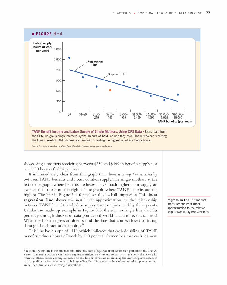
shows, single mothers receiving between $250 and $499 in benefits supply justover 600 hours of labor per year.

It is immediately clear from this graph that there is a negative relationshipbetween TANF benefits and hours of labor supply. The single mothers at theleft of the graph, where benefits are lowest, have much higher labor supply onaverage than those on the right of the graph, where TANF benefits are thehighest. The line in Figure 3-4 formalizes this eyeball impression. This linearregression line shows the best linear approximation to the relationshipbetween TANF benefits and labor supply that is represented by these points.Unlike the made -up example in Figure 3-3, there is no single line that fitsperfectly through this set of data points; real -world data are never that neat!What the linear regression does is find the line that comes closest to fittingthrough the cluster of data points.9

This line has a slope of –110, which indicates that each doubling of TANFbenefits reduces hours of work by 110 per year (remember that each segment


TANF Benefit Income and Labor Supply of Single Mothers, Using CPS Data • Using data fromthe CPS, we group single mothers by the amount of TANF income they have. Those who are receivingthe lowest level of TANF income are the ones providing the highest number of work hours.

Source: Calculations based on data from Current Population Survey’s annual March supplements.

1,800

1,500

1,200

900

600

300

0

Labor supply(hours of work

per year)

$0 $100–249

$250–499

$500–999

$1,000–2,499

$2,500–4,999

$5,000–9,999

$10,000–25,000

$1–99

TANF benefits (per year)

Regressionline

Slope = –110

■ FIGURE 3-4

regression line The line thatmeasures the best linearapproximation to the relation-ship between any two variables.

9 Technically, this line is the one that minimizes the sum of squared distances of each point from the line. Asa result, one major concern with linear regression analysis is outliers. An outlier, which is a point that is very farfrom the others, exerts a strong influence on this line, since we are minimizing the sum of squared distances,so a large distance has an exponentially large effect. For this reason, analysts often use other approaches thatare less sensitive to such outlying observations.

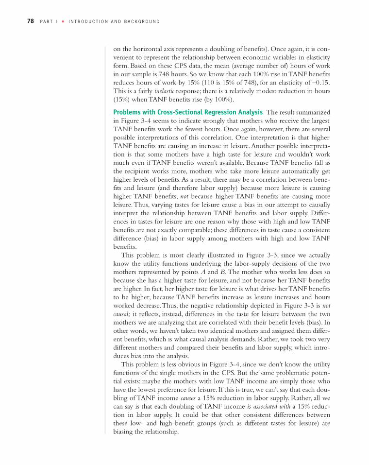
on the horizontal axis represents a doubling of benefits). Once again, it is con-venient to represent the relationship between economic variables in elasticityform. Based on these CPS data, the mean (average number of) hours of workin our sample is 748 hours. So we know that each 100% rise in TANF benefitsreduces hours of work by 15% (110 is 15% of 748), for an elasticity of –0.15.This is a fairly inelastic response; there is a relatively modest reduction in hours(15%) when TANF benefits rise (by 100%).

Problems with Cross-Sectional Regression Analysis The result summarizedin Figure 3-4 seems to indicate strongly that mothers who receive the largestTANF benefits work the fewest hours. Once again, however, there are severalpossible interpretations of this correlation. One interpretation is that higherTANF benefits are causing an increase in leisure. Another possible interpreta-tion is that some mothers have a high taste for leisure and wouldn’t workmuch even if TANF benefits weren’t available. Because TANF benefits fall asthe recipient works more, mothers who take more leisure automatically gethigher levels of benefits. As a result, there may be a correlation between bene-fits and leisure (and therefore labor supply) because more leisure is causinghigher TANF benefits, not because higher TANF benefits are causing moreleisure. Thus, varying tastes for leisure cause a bias in our attempt to causallyinterpret the relationship between TANF benefits and labor supply. Differ-ences in tastes for leisure are one reason why those with high and low TANFbenefits are not exactly comparable; these differences in taste cause a consistentdifference (bias) in labor supply among mothers with high and low TANFbenefits.

This problem is most clearly illustrated in Figure 3-3, since we actuallyknow the utility functions underlying the labor -supply decisions of the twomothers represented by points A and B. The mother who works less does sobecause she has a higher taste for leisure, and not because her TANF benefitsare higher. In fact, her higher taste for leisure is what drives her TANF benefitsto be higher, because TANF benefits increase as leisure increases and hoursworked decrease. Thus, the negative relationship depicted in Figure 3-3 is notcausal; it reflects, instead, differences in the taste for leisure between the twomothers we are analyzing that are correlated with their benefit levels (bias). Inother words, we haven’t taken two identical mothers and assigned them differ-ent benefits, which is what causal analysis demands. Rather, we took two verydifferent mothers and compared their benefits and labor supply, which intro-duces bias into the analysis.

This problem is less obvious in Figure 3-4, since we don’t know the utilityfunctions of the single mothers in the CPS. But the same problematic poten-tial exists: maybe the mothers with low TANF income are simply those whohave the lowest preference for leisure. If this is true, we can’t say that each dou-bling of TANF income causes a 15% reduction in labor supply. Rather, all wecan say is that each doubling of TANF income is associated with a 15% reduc-tion in labor supply. It could be that other consistent differences betweenthese low - and high -benefit groups (such as different tastes for leisure) arebiasing the relationship.


Q

Control Variables Regression analysis has one potential advantage over cor-relation analysis in dealing with the problem of bias: the ability to includecontrol variables. Suppose that the CPS had a variable included in the dataset called “taste for leisure” that accurately reflected each individual’s taste forleisure. Suppose that this variable came in two categorical values: “prefersleisure” and “prefers work,” and that everyone within each of these categoricalvalues had identical tastes for leisure and work. That is, there is no bias withinthese groups, only across them; within each group, individuals are identical interms of their preferences toward work and leisure.

If we had this information, we could divide our sample into two groupsaccording to this leisure variable, and redo the analysis within each group.Within each group, different tastes for leisure cannot be the source of the rela-tionship between TANF benefits and labor supply, because tastes for leisure areidentical within each group. This “taste for leisure” control variable will allowus to get rid of the bias in our comparison, because within each group we nolonger have a systematic difference in tastes for leisure that is correlated withbenefits. Control variables in regression analysis play this role: they try to con-trol for (take into account) other differences across individuals in a sample, sothat any remaining correlation between the dependent variable (e.g., laborsupply) and independent variable (e.g., TANF benefits) can be interpreted as acausal effect of benefits on work.

In reality, control variables are unlikely to ever solve this problem com-pletely, as the key variables we want, such as the intrinsic taste for leisure inthis example, are impossible to measure in data sets. Usually, we have toapproximate the variables we really want, such as taste for leisure, with what isavailable, such as age or education or work experience. These are imperfectproxies, however, so they don’t fully allow us to control for differences in tastefor leisure across the population (e.g., even within age or education or workexperience groups, there will be individuals with very different tastes forleisure). Thus, it is hard to totally get rid of bias with control variables, sincecontrol variables only represent in a limited way the underlying differencesbetween treatment and control groups. We discuss this point in the appendixto this chapter, which includes reference to data on our Web site that you canuse to conduct your own regression analysis.

Quick Hint For many empirical analyses, there will be one clear treatment

group and one clear control group, as in the ERT case. For other analyses, such

as our cross -sectional TANF analysis, there are many groups to be compared with

one another. A cross -sectional regression essentially compares each point in

Figure 3-4 with the other points in order to estimate the relationship between

TANF benefits and labor supply.

Even though the treatment/control analogy is no longer exact, however, the

general intuition remains. It is essential in all empirical work to ensure that

there are no factors that cause consistent differences in behavior (labor supply)

across two groups and are also correlated with the independent variable (TANF


control variables Variablesthat are included in cross -sectional regression models toaccount for differences betweentreatment and control groupsthat can lead to bias.

benefits). When there are more than two groups, the concern is the same: to

ensure that there is no consistent factor that causes groups with higher benefits

to supply less labor than groups with lower benefits, other than the benefit dif-

ferences themselves.

Quasi-ExperimentsAs noted earlier, public finance researchers cannot set up randomized trialsand run experiments for every important behavior that matters for public pol-icy. We have examined alternatives to randomized trials such as time series andcross -sectional regression analysis, but have also seen that these research meth-ods have many shortcomings which make it hard for them to eliminate thebias problem. Is there any way to accurately assess causal influences withoutusing a randomized trial? Is there an alternative to the use of control variablesfor purging empirical models of bias?

Over the past two decades, empirical research in public finance has becomeincreasingly focused on one potential middle -ground solution: the quasi-experiment, a situation that arises naturally when changes in the economicenvironment (such as a policy change) create nearly identical treatment andcontrol groups that can be used to study the effect of that policy change. In aquasi-experiment, outside forces (such as those instituting the policy change)do the randomization for us.

For example, suppose that we have a sample with a large number of singlemothers in the neighboring states of Arkansas and Louisiana, for two years,1996 and 1998. Suppose further that, in 1997, the state of Arkansas cut itsbenefit guarantee by 20%, while Louisiana’s benefits remained unchanged. Inprinciple, this alteration in the states’ policies has essentially performed ourrandomization for us. The women in Arkansas who experienced the decreasein benefits are the treatment group, and the women in Louisiana whose bene-fits did not change are the control. By computing the change in labor supplyacross these groups, and then examining the difference between treatment(Arkansas) and control (Louisiana), we can obtain an estimate of the impact ofbenefits on labor supply that is free of bias.

In principle, of course, we could learn about the effect of this policy changeby simply studying the experience of single mothers in Arkansas. If nothingdiffered between the set of single mothers in the state in 1996 and the set ofsingle mothers in the state in 1998, other than the benefits reduction, then anychange in labor supply would reflect only the change in benefits, and theresults would be free of bias. In practice, such a comparison typically runs intothe problems we associate with time series analysis. For example, the periodfrom 1996 through 1998 was a period of major national economic growth,with many more job openings for low -skilled workers, which could leadsingle mothers to leave TANF and increase their earnings even in the absenceof a benefits change. Thus, it is quite possible that single mothers in Arkansasmay have increased their labor supply even if their benefits had not fallen.


quasi-experiments Changesin the economic environmentthat create nearly identical treat-ment and control groups forstudying the effect of that envi-ronmental change, allowing pub-lic finance economists to takeadvantage of randomization cre-ated by external forces.

Because other factors may have changed that affected the labor supplydecisions of single mothers in Arkansas, the quasi -experimental approachincludes the extra step of comparing the treatment group for whom the policychanged to a control group for whom it did not. The state of Louisiana didnot change its TANF guarantee between 1996 and 1998, but single mothers inLouisiana benefited from the same national economic boom as did those inArkansas. If the increase in labor supply among single mothers in Arkansas isdriven by economic conditions, then we should see the same increase in laborsupply among single mothers in Louisiana; if the increase in labor supplyamong single mothers in Arkansas is driven by lower TANF benefits, then wewould see no change among single mothers in Louisiana. The bias introducedinto our comparison of single mothers in Arkansas in 1996 to single mothersin Arkansas in 1998 by the improvement in economic conditions across thenation is also present when we do a similar comparison within Louisiana. InLouisiana, however, the treatment effect of a higher TANF benefit is notpresent. In this comparison, we can say that:

Hours (Arkansas, 1998) � Hours (Arkansas, 1996) � Treatment effect � Biasfrom economic boom

Hours (Louisiana, 1998) � Hours (Louisiana, 1996) � Bias from economicboom

Difference � Treatment effect

By subtracting the change in hours of work in Louisiana (the control group)from the change in hours of work in Arkansas (the treatment group), we con-trol for the bias caused by the economic boom and obtain a causal estimate ofthe effect of TANF benefits on hours of work.

Table 3-1 provides an illustrative but hypothetical set of numbers that wecan use to analyze the results of this quasi -experiment. Suppose that the welfareguarantee was cut from $5,000 to $4,000 in Arkansas between 1996 and 1998.Over the same period, hours of work per year among single mothers in thestate rose by from 1,000 to 1,200. The time series estimate using the experi-ence of Arkansas alone would be that the $1,000 benefit reduction (20%)increased hours of work by 200 (20%). This outcome implies an elasticity oftotal hours with respect to benefits of �1 (a 20% benefit cut led to a 20% laborsupply rise). Notice that this estimate is considerably larger than the �0.67elasticity found in the randomized trial in California (our gold standard).

Consider now the bottom panel of Table 3-1. This panel shows that,between 1996 and 1998, there was no change in welfare benefits in Louisiana,but hours of work increased by 50 hours per year. Thus, it appears that theeconomic boom did play a role in the increase in hours worked by singlemothers. By looking only at time series data from Arkansas, we ignore theeffect of the economic boom. If we don’t take this effect into account in ourstudy, our conclusions about the effect of TANF benefits on labor supply willbe biased.

A simple solution to this problem, as we have seen, is to examine the differ-ence between the change in Arkansas and the change in Louisiana. That is,


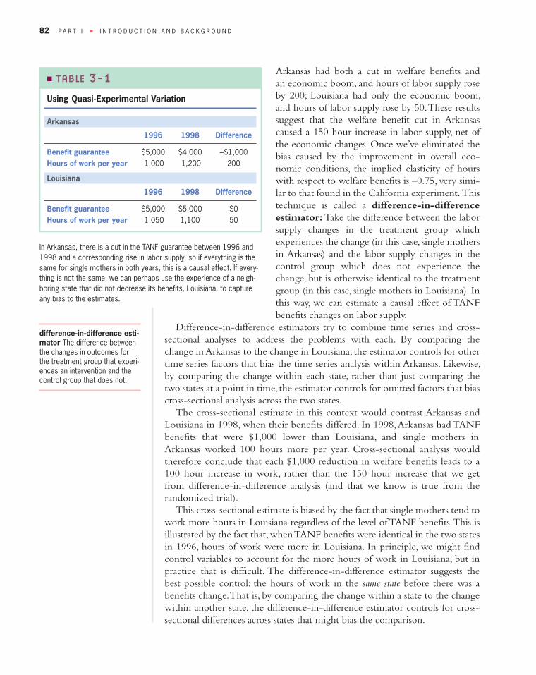
Arkansas had both a cut in welfare benefits andan economic boom, and hours of labor supply roseby 200; Louisiana had only the economic boom,and hours of labor supply rose by 50. These resultssuggest that the welfare benefit cut in Arkansascaused a 150 hour increase in labor supply, net ofthe economic changes. Once we’ve eliminated thebias caused by the improvement in overall eco-nomic conditions, the implied elasticity of hourswith respect to welfare benefits is –0.75, very simi-lar to that found in the California experiment. Thistechnique is called a difference -in-differenceestimator: Take the difference between the laborsupply changes in the treatment group whichexperiences the change (in this case, single mothersin Arkansas) and the labor supply changes in thecontrol group which does not experience thechange, but is otherwise identical to the treatmentgroup (in this case, single mothers in Louisiana). Inthis way, we can estimate a causal effect of TANFbenefits changes on labor supply.

Difference -in-difference estimators try to combine time series and cross -sectional analyses to address the problems with each. By comparing thechange in Arkansas to the change in Louisiana, the estimator controls for othertime series factors that bias the time series analysis within Arkansas. Likewise,by comparing the change within each state, rather than just comparing thetwo states at a point in time, the estimator controls for omitted factors that biascross -sectional analysis across the two states.

The cross -sectional estimate in this context would contrast Arkansas andLouisiana in 1998, when their benefits differed. In 1998, Arkansas had TANFbenefits that were $1,000 lower than Louisiana, and single mothers inArkansas worked 100 hours more per year. Cross -sectional analysis wouldtherefore conclude that each $1,000 reduction in welfare benefits leads to a100 hour increase in work, rather than the 150 hour increase that we getfrom difference -in-difference analysis (and that we know is true from therandomized trial).

This cross -sectional estimate is biased by the fact that single mothers tend towork more hours in Louisiana regardless of the level of TANF benefits. This isillustrated by the fact that, when TANF benefits were identical in the two statesin 1996, hours of work were more in Louisiana. In principle, we might findcontrol variables to account for the more hours of work in Louisiana, but inpractice that is difficult. The difference -in-difference estimator suggests thebest possible control: the hours of work in the same state before there was abenefits change. That is, by comparing the change within a state to the changewithin another state, the difference -in-difference estimator controls for cross -sectional differences across states that might bias the comparison.


In Arkansas, there is a cut in the TANF guarantee between 1996 and1998 and a corresponding rise in labor supply, so if everything is thesame for single mothers in both years, this is a causal effect. If every-thing is not the same, we can perhaps use the experience of a neigh-boring state that did not decrease its benefits, Louisiana, to captureany bias to the estimates.

■ TABLE 3-1Using Quasi-Experimental Variation

Arkansas

1996 1998 Difference

Benefit guarantee $5,000 $4,000 –$1,000Hours of work per year 1,000 1,200 200

Louisiana

1996 1998 Difference

Benefit guarantee $5,000 $5,000 $0Hours of work per year 1,050 1,100 50

difference -in-difference esti-mator The difference betweenthe changes in outcomes forthe treatment group that experi-ences an intervention and thecontrol group that does not.

Problems with Quasi -Experimental Analysis As well as the difference -in-difference quasi -experimental approach works to control for bias, it is still lessthan ideal. Suppose, for example, that the economic boom of this periodaffected Arkansas in a different way than it affected Louisiana. If this were true,then the “bias from economic boom” terms in the previous comparisonwould not be equal, and we would be unable to isolate the treatment effect ofhigher TANF benefits by simple subtraction. Instead, we get a new bias term:the difference in the impact of the economic boom in Arkansas and Louisiana.That is, when we compute our difference -in-difference estimator we obtain:

Hours (Arkansas, 1998) � Hours (Arkansas, 1996) � AR bias from economicboom � Treatment

Hours (Louisiana, 1998) � Hours (Louisiana, 1996) � LA bias fromeconomic boom

Difference � Treatment effect �(AR bias – LA bias)

Since AR and LA biases are not equal, the estimator will not identify the truetreatment effect.

With quasi -experimental studies, unlike true experiments, we can never becompletely certain that we have purged all bias from the treatment–controlcomparison. Quasi -experimental studies use two approaches to try to makethe argument that they have obtained a causal estimate. The first is intuitive:trying to argue that, given the treatment and control groups, it seems verylikely that bias has been removed. The second is statistical: to continue to usealternative or additional control groups to confirm that the bias has beenremoved. In the appendix to Chapter 14, we discuss how alternative or addi-tional control groups can be used to confirm the conclusions of quasi -experimental analysis.

Structural ModelingThe randomized trials and quasi -experimental approaches previously describedhave the distinct advantage that, if applied appropriately, they can address thedifficult problem of distinguishing causality from correlation. Yet they alsohave two important limitations. First, they only provide an estimate of thecausal impact of a particular treatment. That is, the California experiment foundthat cutting benefits by 15% raised employment rates by 4.5 percentage points.This is the best estimate of the impact of cutting benefits by 15%, but it maynot tell us much about the impact of cutting benefits by 30%, or of raisingbenefits by 15%. That is, we can’t necessarily extrapolate from a particularchange in the environment to model all possible changes in the environment.These approaches give us a precise answer to a specific question, but don’tnecessarily provide a general conclusion about how different changes in bene-fits might affect behavior.

The second limitation is that these approaches can tell us how outcomeschange when there is an intervention, but often they cannot tell us why. Consider


the behavior of mothers with income between $6,000 and $10,000 in ourexample from Chapter 2, and how the mothers react to a cut in benefits underTANF. For these mothers, as we noted, there is both an income effect and asubstitution effect leading to more work; both mothers are poorer becausebenefits have fallen, and they have a higher net wage since the implicit tax ratehas fallen. An experimental or quasi -experimental study of the responses ofthese women to the benefits reduction might show us the total effect of thereduction on their labor supply, but it would tell us very little about the rela-tive importance of these income and substitution effects.

Yet, as we will learn later in this book, we often care about the structuralestimates of labor supply responses, the estimates that tell us about features ofutility that drive individual decisions, such as substitution and income effects.Randomized or quasi -experimental estimates provide reduced form estimatesonly. Reduced form estimates show the impact of one particular change onoverall labor -supply responses. This second disadvantage of randomized orquasi-experiments is thus related to the first: if we understood the underlyingstructure of labor -supply responses, it might be possible to say more about howlabor supply would respond to different types of policy interventions.

These issues have led to the vibrant field of structural estimation. Using thisresearch approach, empirical economists attempt to estimate not just reducedform responses to the environment but the actual underlying features of utilityfunctions. They do so by more closely employing the theory outlined in theprevious chapter to develop an empirical framework that not only estimatesoverall responses, but also decomposes these responses into, for example, sub-stitution and income effects.

Structural models potentially provide a very useful complement to experi-mental or quasi -experimental analyses. Yet structural models are often moredifficult to estimate than reduced form models because both use the sameamount of information, yet structural models are used to try to learn muchmore from that information. Consider the TANF example. The earlier analysisshowed you how to derive a reduced form estimate of the impact of a changein TANF benefits. Using this same information to decompose that responseinto income and substitution effects is not possible employing the same simpleapproach. Rather, that decomposition is only possible if the researcher assumesa particular form for the utility function, as we did in Chapter 2, and thenemploys that assumption to decompose the overall response into its two com-ponents. If the assumption for the form of the utility function is correct, thenthis approach provides more information. If it is incorrect, however, then theresponse derived from this approach might lead one to incorrectly estimateincome and substitution effects.

From the perspective of this text, reduced form estimation has one otheradvantage (which may be obvious after reading this section!): it is much easierto think about and explain. Thus, for the remainder of the text, we will largelyrely on reduced form modeling and evidence when discussing empiricalresults in public finance. Yet the promise of structural modeling should not bediscounted, and is a topic of fruitful future study for those of you who want togo on in economics. The lessons about empirical work learned in this book


structural estimates Esti-mates of the features that driveindividual decisions, such asincome and substitution effectsor utility parameters.

reduced form estimatesMeasures of the total impact ofan independent variable on adependent variable, withoutdecomposing the source of thatbehavior response in terms ofunderlying utility functions.

are universal for all types of studies; they provide a basis that you can takeforward to more sophisticated empirical approaches such as structuralmodeling.

3.4Conclusion

The central issue for any policy question is establishing a causal relationshipbetween the policy in question and the outcome of interest. Do lower

welfare benefits cause higher labor supply among single mothers? Does morepollution in the air cause worse health outcomes? Do larger benefits for unem-ployment insurance cause individuals to stay unemployed longer? These are thetypes of questions that we will address in this book using the empirical methodsdescribed here.

In this chapter, we discussed several approaches to distinguish causality fromcorrelation. The gold standard for doing so is the randomized trial, whichremoves bias through randomly assigning treatment and control groups.Unfortunately, however, such trials are not available for every question wewish to address in empirical public finance. As a result, we turn to alternativemethods such as time series analysis, cross -sectional regression analysis, and quasi -experimental analysis. Each of these alternatives has weaknesses, but carefulconsideration of the problem at hand can often lead to a sensible solution tothe bias problem that plagues empirical analysis.


are identical by definition, there is no bias, and anydifferences across the groups are a causal effect.

■ Time series analysis is unlikely to provide a con-vincing estimate of causal effects because so manyother factors change through time.

■ Cross -sectional regression analysis also suffers frombias problems because similar people make differentchoices for reasons that can’t be observed, leadingonce again to bias. Including control variables offersthe potential to address this bias.

■ Quasi-experimental methods have the potential toapproximate randomized trials, but control groupsmust be selected carefully in order to avoid biasedcomparisons.

■ A primary goal of empirical work is to document thecausal effects of one economic factor on another, forexample the causal effect of raising TANF benefitson the labor supply of single mothers.

■ The difficulty with this goal is that it requires treat-ment groups (those who are affected by policy) andcontrol groups (those not affected) who are identicalexcept for the policy intervention.

■ If these groups are not identical, there can be bias—that is, other consistent differences across treatment/control groups that are correlated with, but not dueto, the treatment itself.

■ Randomized trials are the gold standard to sur-mount this problem. Since treatments and controls

� H I G H L I G H T S

two groups and find that the treatment group hasa lower average age than the control group. Howcould this arise?

1. Suppose you are running a randomized experi-ment and you randomly assign study participantsto control and treatment groups. After making theassignments, you study the characteristics of the

� Q U E S T I O N S A N D P R O B L E M S

2. Why is a randomized trial the “gold standard” forsolving the identification problem?

3. What do we mean when we say that correlationdoes not imply causality? What are some of theways in which an empirical analyst attempts todisentangle the two?

4. A researcher conducted a cross -sectional analysisof children and found that the average test per-formance of children with divorced parents waslower than the average test performance of chil-dren of intact families. This researcher then con-cluded that divorce is bad for children’s testoutcomes. What is wrong with this analysis?

5. A study in the Annals of Improbable Research oncereported that counties with large numbers ofmobile-home parks had higher rates of tornadoesthan the rest of the population. The authors con-clude that mobile -home parks cause tornadooccurrences. What is an alternative explanation forthis fact?

6. What are some of the concerns with conductingrandomized trials? How can quasi -experimentspotentially help here?

7. You are hired by the government to evaluate theimpact of a policy change that affects one groupof individuals but not another. Suppose thatbefore the policy change, members of a groupaffected by the policy averaged $17,000 in earn-ings and members of a group unaffected by thepolicy averaged $16,400. After the policy change,


members of the affected group averaged $18,200in earnings while members of the unaffected groupaveraged $17,700 in earnings.

a. How can you estimate the impact of the policychange? What is the name for this type of esti-mation?

b. What are the assumptions you have to makefor this to be a valid estimate of the impact ofthe policy change?

8. Consider the example presented in the appendixto this chapter. Which coefficient estimates wouldbe considered “statistically significant” or distinctfrom zero?

9. A researcher wants to investigate the effects ofeducation spending on housing prices, but sheonly has cross -sectional data. When she performsher regression analysis, she controls for averageJanuary and July temperatures. Why is she doingthis? What other variables would you control for,and why?

10. It is commonly taught in introductory microeco-nomics courses that minimum wages cause unem-ployment. The Federally mandated minimumwage is $7.25, but approximately 1/3 of stateshave higher state -mandated minimum wages.Why can’t you test the “minimum wages causeunemployment” theory by simply comparingunemployment rates across states with differentminimum wages? Can you think of a better wayto test it?

� A DVA N C E D Q U E S T I O N S

11. Suppose that your friend Oscar has collected dataand determined that towns with newly construct-ed high schools tend to have higher SAT scoresthan other towns. He tells you that he has provedthat new high schools cause higher SAT scores.When you object that “correlation does not implycausation,” he is ready with more data. He showsyou convincing evidence that SAT scores tend toincrease shortly after towns build new highschools, but that there is no tendency for newhigh schools to be built in towns which haverecently seen large increases in SAT scores. Is this

enough evidence to prove that new high schoolscause higher SAT scores, or can you think of analternative explanation for Oscar’s data?

12. Researchers often use panel data (multiple obser-vations over time of the same people) to conductregression analysis. With these data, researchersare able to compare the same person over time inorder to assess the impacts of policies on individ-ual behavior. How could this provide an improve-ment over cross -sectional regression analysis of thetype described in the text?

13. Suppose that your state announced that it wouldprovide free tuition to high -achieving studentsgraduating from high school starting in 2007. Youdecide to see whether this new program inducesfamilies with high -achieving children graduatingin 2007 or later to purchase new cars. To test yourfindings, you use a “falsification exercise”: youobserve the new -car-purchasing behavior of fam-ilies with children graduating in 2006. Why is thisa useful exercise?

14. Your state introduced a tax cut in the year 1999.You are interested in seeing whether this tax cuthas led to increases in personal consumptionwithin the state.

You observe the following information:


a. Your friend argues that the best estimate of theeffect of the tax cut is an increase in consump-tion of 30 units, but you think that the trueeffect is smaller, because consumption wastrending upward prior to the tax cut. What doyou think is a better estimate?

b. Suppose that you find information on a neigh-boring state that did not change its tax policyduring this time period. You observe the fol-lowing information in that state:

Year Consumption in your state

1994 3001996 3101998 3202000 350

Year Consumption in neighboring state

1994 2601996 2701998 2802000 300

Given this information, what is your best esti-mate of the effect of the tax cut on consump-tion? What assumptions are required for that tobe the right estimate of the effect of the taxcut? Explain.

88

Cross -Sectional RegressionAnalysis

Appendix to Chapter 3

In the text, we presented a cursory discussion of cross -sectional regressionanalysis, and the role of control variables. In this appendix, we provide amore detailed presentation of this approach within our TANF example.

Data For this analysis, we use data from the March 2002 Current PopulationSurvey (CPS). From that survey, we selected all women who reported thatthey were unmarried and had a child younger than age 19. The total sample is8,024 single mothers.

For this sample, we have gathered data on the following variables for eachwoman:

� TANF: Total cash TANF benefits in the previous year (in thousands ofdollars).

� Hours: Total hours of work in the previous year, computed as reportedweeks of work times usual hours per week.

� Race: We divide reported race into white, black, and other.� Age: Age in years.� Education: We use reported education to divide individuals into four

groups: high school dropouts; high school graduates with no college;those with some college; and college graduates.

� Urbanicity: We use information on residential location to divide individ-uals into four groups: central city; other urban; rural; and unclear (theCPS doesn’t identify location for some mothers for survey confidential-ity reasons).

Regression Using these data, we can estimate a regression of the impact ofwelfare on hours of work of the form:

(1) HOURSi � α � βTANFi � i

where there is one observation for each mother i. This is the counterpart of theregression analysis shown in Figure 3-4, but now we are using each individualdata point, rather than grouping the data into categories for convenience.

In this regression, α, the constant term, represents the estimated number ofhours worked if welfare benefits are zero. β is the slope coefficient, which

∋

represents the change in hours worked per dollarof welfare benefits. is the error term, which rep-resents the difference for each observation betweenits actual value and its predicted value based onthe model.

The results of estimating this regression modelare presented in the first column of the appendixtable. The first row shows the constant term α,which is 1,537: this measures the predicted hoursof labor supply delivered at zero welfare benefits.The second row shows the coefficient β, which is�107: each $1,000 of welfare benefits lowershours worked by 107. This is very close to the esti-mate from the grouped data of �110 discussed inthe text. Thus, for a mother with no welfare bene-fits, predicted hours of work are 1,537; for a motherwith $5,000 in welfare benefits, predicted hours ofwork are 1,537 � 5 × 107 � 1,002.

Underneath this estimate in parentheses is theestimate’s standard error. This figure captures the pre-cision with which these coefficients are estimatedand reminds us that we have here only a statisticalrepresentation of the relationship between welfarebenefits and hours worked. Roughly speaking, wecannot statistically distinguish values of β that aretwo standard errors below or above the estimatedcoefficient. In our context, with a standard error of3.7 hours, the results show that our best estimate isthat each thousand dollars of welfare lowers hours worked by 107, but we can’trule out that the effect is only 99.6 (107 � 2 � 3.7) or that it is 114.4 (107 �2 � 3.7).

In the context of empirical economics, this is a very precise estimate. Typi-cally, as long as the estimate is more than twice the size of its standard error,we say that it is statistically significant.

The final row of the table shows the R2 of the regression. This is a measureof how well the statistical regression model is fitting the underlying data. AnR2 of 1 would mean that the data are perfectly explained by the model so thatall data points lie directly on the regression line; an R2 of 0 means that the dataare not at all explained. The value of 0.095 here says that less than 10% of thevariation in the data is explained by this regression model.

As discussed in the text, however, this regression model suffers from seriousbias problems, since those mothers who have a high taste for leisure will haveboth low hours of work and high welfare payments. One approach to address-ing this problem suggested in the text was to include control variables. Wedon’t have the ideal control variable, which is taste for leisure. We do, however,have other variables that might be correlated with tastes for leisure or other

∋


■ APPENDIX 3 TABLE

Cross-Sectional Regression Analysis

Equation (1) Equation (2)

Constant 1,537 2,062(10) (61)

TANF benefits –107 –93(3.7) (3.6)

White 181(44)

Black 61(47)

High school dropout –756(30)

High school graduate –347(25)

Some college –232(28)

Age –9.3(0.8)

Central city –12(30)

Other urban 34(29)

Rural –43(31)

R2 0.095 0.183

factors that determine labor supply: race, education, age, and urbanicity. So wecan estimate regression models of the form:

(2) HOURSi � α � βTANFi � δCONTROLi � i

where CONTROL is the set of control variables for individual i.In the second column of the appendix table, we show the impact of includ-

ing these other variables. When we have a categorical variable such as race(categorized into white, black, and other), we include indicator variables thattake on a value of 1 if the individual is of that race, and 0 otherwise. Note thatwhen we have N categories for any variable (e.g., 3 categories for race),we only include N � 1 indicator variables, so that all estimates are relative tothe excluded category (e.g., the coefficient on the indicator for “black” shows theimpact of being black on welfare income, relative to the omitted group ofHispanics).

Adding these control variables does indeed lower the estimated impact ofwelfare benefits on labor supply. The coefficient falls to –93, but remains highlysignificant. The R2 doubles but still indicates that we are explaining less than20% of the variation in the data.

The control variables are themselves also of interest:� Race: Whites are estimated to work 181 hours per year more than His-

panics (the omitted group); blacks are estimated to work 61 hours peryear more than Hispanics, but this estimate is only about 1.3 times aslarge as its standard error, so we do not call this a statistically significantdifference.

� Education: Hours of work clearly rise with education. High schooldropouts work 756 fewer hours per year than do college graduates (theomitted group); high school graduates work 347 fewer hours per year;and those with some college work 232 fewer hours per year than thosewho graduate from college. All of these estimates are very precise (thecoefficients are very large relative to the standard errors beneath themin parentheses).

� Age: Hours worked decline with age, with each year of age leading to 9 fewer hours of work; this is a very precise estimate as well.

� Location: Relative to those with unidentified urbanicity, people in citiesand rural areas work less and those in the suburbs work more, but noneof these estimates is statistically precise.

Do these control variables eliminate bias in the estimated relationshipbetween TANF benefits and labor supply? There is no way to know for sure,but it seems unlikely. The fact that this large set of controls explains only 9%more of the variation in labor supply across individuals suggests that it isunlikely to capture all of the factors correlated with both labor supply andTANF benefits.

∋


publiic finance and public policy - humboldt state...

Documents