pullback attracting inertial manifolds for nonautonomous dynamical systems

889

1040-7294/02/1000-0889/0 © 2002 Plenum Publishing Corporation

Journal of Dynamics and Differential Equations, Vol. 14, No. 4, October 2002 (© 2002)

Pullback Attracting Inertial Manifolds forNonautonomous Dynamical Systems

Norbert Koksch1 and Stefan Siegmund2 , 3

1 Fachrichtung Mathematik, Technische Universität Dresden, 01062 Dresden, Germany. E-mail:[email protected] Institute for Mathematics and its Applications, University of Minnesota, Minneapolis,

Minnesota 55455. E-mail: [email protected] To whom correspondence should be addressed.

Received April 29, 2002

In this paper we present an abstract approach to inertial manifolds for nonau-tonomous dynamical systems. Our result on the existence of inertial manifoldsrequires only two geometrical assumptions, called cone invariance and squeez-ing property, and two additional technical assumptions, called boundedness andcoercivity property. Moreover we give conditions which ensure that the globalpullback attractor is contained in the inertial manifold. In the second part of thepaper we consider special nonautonomous dynamical systems, namely processes(or two-parameter semi-flows). As a first application of our abstract approachand for reason of comparison with known results we verify the assumptions forsemilinear nonautonomous evolution equations whose linear part satisfies anexponential dichotomy condition and whose nonlinear part is globally boundedand globally Lipschitz.

KEY WORDS: Inertial manifolds; pullback attractors; nonautonomous dynami-cal systems.

1. INTRODUCTION

Let us consider a dissipative nonlinear evolution equation of the form

u+Au=f(u)

in a Banach space X, where A is a linear sectorial operator with compactresolvent and f is a nonlinear function. Such an evolution equation may be

an ordinary differential equation (X=Rn) or the abstract formulation of asemilinear parabolic differential equation with X as a suitable functionspace over the spatial domain. In the last case, A corresponds to a lineardifferential operator and f is a nonlinearity which may involve derivativesof lower order than A.

The dissipativity finds its expression in the fact that there is a boundedset A in X which absorbs bounded subsets of the phase space after a finitetime. Given a compact set A which is absorbing and positively invariantwith respect to the semi-flow, the w-limit set of A under the semi-flow hassome interesting properties: There is a compact, invariant set A in A

which attracts all trajectories. Such a set A is called the global attractor[Tem97], and it is maximal in the sense that it is the largest set with thisproperty. Often global attractors have a finite (fractal) dimension and,therefore, they are important objects for the study of long time behavior.At the present level of understanding of dynamical systems, the attractorsare expected to be very complicated objects (fractals) and their practicalutilization, for instance for numerical simulations, may be difficult. Becauseof the finite dimensionality of the attractor, it is a natural question if theattractor could be generated by a (possibly high dimensional) system ofordinary differential equations, i.e., if the flow on the attractor could begenerated by a system of ordinary differential equations. An indirect wayto obtain such a system is to embed the attractor A into a smooth finitedimensional manifold.

Inertial manifolds are positively invariant, exponentially attracting,finite dimensional Lipschitz manifolds. For an introduction see Sell andYou [SY02]. They go back to R. Mane, D. Henry, X. Mora, and D. A.Kamaev [Hen81, Mor83, Man77, Kam84] and were first introducedand studied by P. Constantin, C. Foias, B. Nicoalenko, G. R. Sell, andR. Temam [FST85, FNST85, CFNT86] for selfadjoint A. For the con-struction of inertial manifolds with A being non-selfadjoint see for example[SY92] and [Tem97]. Inertial manifolds are generalizations of center-unstable manifolds and they are more convenient objects which capture thelong-time behavior of dynamical systems. If such a manifold exists, then itcontains the global attractor A. Usually an inertial manifold M is soughtas the graph of a sufficiently smooth function m on PX, i.e.,

M=graph(m) :={x+m(x) : x ¥ PX},

where P is a finite dimensional projector. The finite dimensionality and theexponential attracting property permit the reduction of the dynamics of the

890 Koksch and Siegmund

infinite or high dimensional equation to the dynamics of a finite or lowdimensional ordinary differential equation

x+Ax=Pf(x+m(x)) in PX

called inertial form system. A stronger reduction property is the exponentialtracking property [FST89], also called asymptotical completeness property[Rob96]: Each trajectory of the evolution equation tends exponentiallyto a trajectory in the inertial manifold.

Thus, one can reduce (in some sense) an infinite-dimensional physicalsystem to a system with a finite number of degrees of freedom and useknown properties of ordinary differential equations in Rn for the qualita-tive analysis of the behavior of the solutions of the original equation forlarge time. Another advantage of studying the inertial form system is thereduction of the dimension of the original problem which could be impor-tant for the numerical analysis. In concrete applications, the N-dimensionalprojector P is the projector onto the eigenspace spanned by the first NFourier modes of L, i.e., by eigenvectors of A belonging to the set of the Nsmallest eigenvalues of A. Hence the inertial form system describes thedynamics of the slow modes. For applications of the concept of inertialmanifolds see for example [HR92, RB95, SK95, BH96, MSZ00].

There are a few ways of constructing an inertial manifold. Most ofthem are generalizations of methods developed for the construction ofunstable, center-unstable or center manifolds for ordinary differentialequations. Following the introduction of [Wig94], there are at least thefollowing two basic methods:

The Lyapunov–Perron method has been developed by A. M. Lyapunov[Lya47, Lya92] and O. Perron [Per28, Per29, Per30] for the proof ofthe existence of stable and unstable manifolds of hyperbolic equilibriumpoints. In the context of ordinary differential equations, it deals with theintegral equation formulation of the differential equation and constructsthe invariant manifold as a fixed point of an operator that is derived fromthis integral equation. This method has been used in many different situa-tions. The book of J. Hale [Hal80] may serve as a good reference. In theinfinite dimensional setting, the method is used by D. Henry [Hen81] toprove the existence of stable, unstable and center manifolds for semilinearparabolic equations. In [FST88, Tem88, CFNT89b, FST89, DG91], it hasbeen adapted for the construction of inertial manifolds. At the moment,the Lyapunov–Perron method is the most common method for inertialmanifolds.

Hadamard’s method [Had01], also called graph transformationmethod, has been developed to prove the existence of stable and unstable

Pullback Attracting Inertial Manifolds 891

manifolds of fixed points of diffeomorphisms. The graph transformationmethod is more geometrical in nature than the Lyapunov–Perron method.In presence of a hyperbolic fixed point, the stable and unstable manifoldsare constructed as graphs over the linearized stable and unstable subspaces.Mallet–Paret and Sell [MPS88] were the first who used Hadamard’smethod for the construction of inertial manifolds, see also [BJ89, Rob93,Rob01]. A review on different construction methods (including Hadamard’smethod) for inertial manifolds can be found in [LS89, Nin93].

The above mentioned notion of inertial manifolds is translated andextended to more general classes of differential equations like nonautono-mous differential equations, [GV97, WF97, LL99], retarded parabolic dif-ferential equations, [TY94, BdMCR98], or differential equations withrandom or stochastic perturbations, [Chu95, BF95, CL99, CS01, DLS01].

The construction of inertial manifolds often is redone for differentclasses of equations. Our aim is to separate the general structure of theconstruction from the technical estimates which vary from example toexample. To achieve this goal we develop the existence result of inertialmanifolds on the abstract level of nonautonomous dynamical systems andthen apply it to explicit nonautonomous evolution equations under variousassumptions.

In Section 2 we introduce the abstract notion of a nonautonomousdynamical system extending dynamical systems, to the nonautonomoussituation. For a nonautonomous dynamical system we introduce inertialmanifolds and global pullback attractors. We formulate a cone invariance,squeezing, boundedness and coercivity property which are assumed inSubsection 3.4 where the existence of an inertial manifold is proved.Moreover, we give conditions which imply that the global pullback attrac-tor is contained in the inertial manifold. The assumptions of the existenceresult are formulated on the general level of nonautonomous dynamicalsystems and are independent of a specific equation which generates thenonautonomous dynamical system.

In Section 3 we apply it to special nonautonomous dynamical systems,namely processes (or two-parameter semi-flows). As a first application weverify the assumptions for nonautonomous semilinear evolution equationswhose linear part satisfies an exponential dichotomy condition and whosenonlinear part is globally bounded and globally Lipschitz under theassumption that a special algebraic problem is solvable. For this wedevelop and apply comparison theorems. The algebraic problem is solvableif the exponential rates in the exponential dichotomy condition satisfy agap condition whose form depends on the used Lipschitz inequality and theconcrete form of the exponential dichotomy condition. Finally we compareour results with known ones.


Applications to nonautonomous dynamical systems which are gener-ated by stochastic or retarded partial differential equations are subject of aforthcoming paper.

2. NONAUTONOMOUS DYNAMICAL SYSTEMS

2.1. Preliminaries

Let (X, || · ||) be a Banach space.

Definition 2.1 (Nonautonomous Dynamical System (NDS)). A non-autonomous dynamical system (NDS) on X is a cocycle j over a drivingsystem h on a set B, i.e.,

(i) h: R×BQB is a dynamical system, i.e., the family h(t, · )=h(t):BQB of self-mappings of B satisfies the group property

h(0)=idB, h(t+s)=h(t) p h(s)

for all t, s ¥ R.

(ii) j: R \ 0×B×XQX is a cocycle, i.e., the family j(t, b, · )=j(t, b) : XQX of self-mappings of X satisfies the cocycleproperty

j(0, b)=idX, j(t+s, b)=j(t, h(s) b) p j(s, b)

for all t, s \ 0 and b ¥B. Moreover (t, x)W j(t, b, x) is contin-uous.

Remark 2.2.

(i) The set B is called base and in applications it has additionalstructure, e.g., it is a probability space, a topological space or acompact group and the driving system has additional regularity,e.g., it is ergodic or continuous.

(ii) The pair of mappings

(h, j): R \ 0×B×XQB×X, (t, b, x)W (h(t, b), j(t, b, x))

is a special semi-dynamical system a so-called skew product flow(usually one requires additionally that (h, j) is continuous). IfB={b} consists of one point then the cocycle j is a semi-dynamical system.


(iii) We use the abbreviations htb or h(t) b for h(t, b) and j(t, b) xfor j(t, b, x). We also say that j is an NDS to abbreviate thesituation of Definition 2.1.

Definition 2.3 (Nonautonomous Set). A family M=(M(b))b ¥B ofnonempty sets M(b) …X is called a nonautonomous set and M(b) is calledthe b-fiber of M or the fiber of M over b. We say that M is closed, open,bounded, or compact, if every fiber has the corresponding property. Fornotational convenience we use the identification M 4 {(b, x) : b ¥B,x ¥M(b)} …B×X.

Definition 2.4 (Invariance of Nonautonomous Set). A nonautono-mous set M is called forward invariant under the NDS j, if j(t, b)M(b) …M(htb) for t \ 0 and b ¥B. It is called invariant, if j(t, b)M(b)=M(htb) for t \ 0 and b ¥B.

Definition 2.5 (Inertial Manifold). Let j be an NDS. Then a nonau-tonomous set M is called (nonautonomous) inertial manifold if

(i) every fiber M(b) is a finite-dimensional Lipschitz manifold in X

of dimension N for an N ¥N;

(ii) M is invariant;

(iii) M is exponentially attracting, i.e., there exists a positive constantg such that for every b ¥B and x ¥X there exists an xŒ ¥M(b)with

||j(t, b) x−j(t, b) xŒ|| [Ke−gt for t \ 0 and b ¥B

and a constant K=K(b, x, xŒ) > 0.

The property (iii) is also called exponential tracking property orasymptotic completeness property and xŒ or j( · , b) xŒ is said to be theasymptotic phase of x or j( · , b) x, respectively.

Recall that if D and A are nonempty closed sets in X, the Hausdorffsemi-metric d(D |A) is defined by

d(D |A) :=supx ¥D

d(x,A), d(x,A) := infy ¥A

d(x, y)= infy ¥A

||x−y||.

Now we want to generalize the attractor notion of dynamical systems tononautonomous dynamical systems. A natural generalization of convergence


to a nonautonomous set A seems to be the forwards running convergencedefined by

d(j(t, b) x,A(htb))Q 0 for tQ..

However, this does not ensure convergence to a specific component set A(b)for a fixed b. For that one needs to start ‘‘progressively earlier’’ at h−tbin order to ‘‘finish’’ at b. This leads to the concept of pullback convergencedefined by

d(j(t, h−tb) x,A(b))Q 0 for tQ..

Note that forward and pullback convergence are equivalent for autono-mous dynamical systems.

Using this we can define a pullback attractor.

Definition 2.6 (Pullback Attracting, Absorbing, Attractor). Let j bean NDS and A be a nonautonomous set.

(i) A is called (globally) pullback attracting if for every boundedset D …X and b ¥B

limtQ.d(j(t, h−tb) D |A(b))=0.

(ii) A is called (globally) pullback absorbing if A is bounded andfor every bounded set D …X and b ¥B there is a T > 0 with

j(t, h−tb) D …A(b) for all t \ T.

(iii) A is called (global) pullback attractor of j if A is compact,invariant and pullback attracting.

The concept of pullback convergence was introduced in the mid 1990s inthe context of random dynamical systems (see Schmalfuss [Sch92], Craueland Flandoli [CF94], Flandoli and Schmalfuss [FS96], and Crauel,Debussche and Flandoli [CDF97]) and has been used, e.g., in numericaldynamics, see for example [KS97b, KS97a, KS98]. Note that a similaridea had already been used in the 1960s by Mark Krasnoselski [Kra68] toestablish the existence of solutions that exist and remain bounded on theentire time set.

Now we define a handy notion introduced for random dynamicalsystems (see Ludwig Arnold [Arn98, Definition 4.1.1(ii)]) describingsubexponential growth of a function.


Definition 2.7 (Temperedness). A function R: BQ ] 0,.[ is calledtempered from above if for every b ¥B

lim suptQ ±.

1|t|

log R(htb)=0.

Note that the following characterization holds.

Corollary 2.8. Suppose that R: BQ ] 0,.[ is a nonautonomousvariable. Then the following statements are equivalent:

(i) R is tempered from above.

(ii) For every e > 0 and b ¥B there exists a T > 0 such that

R(htb) [ e e |t| for |t| \ T.

Definition 2.9 (Nonautonomous Projector). Let j be an NDS. A familyp=(p(b))b ¥B of projectors p(b) ¥ L(X, X) in X is called nonautonomousprojector.

(i) p is called tempered from above if bW ||p(b)|| is tempered fromabove.

(ii) p is called N-dimensional for an N ¥N if dim im p(b)=N forevery b ¥B.

2.2. Inertial Manifolds for Nonautonomous Dynamical Systems

Let p1 be an N-dimensional nonautonomous projector in X. We definethe complementary projector

p2(b) :=idX−p1(b) for b ¥B.

Then

X1(b) :=p1(b) X and X2(b) :=p2(b) X, b ¥B

define nonautonomous sets Xi consisting of complementary linear sub-spaces Xi(b) of X, i.e., X1(b) ÀX2(b)=X. For this fact we also writeX1 ÀX2=B×X.

We want to construct a nonautonomous inertial manifold

M=(M(b))b ¥B


consisting of manifolds M(b) which are trivial in the sense that each ofthem can be described by a single chart, i.e.,

M(b)=graph(m(b, · )) :={x1+m(b, x1) : x1 ¥X1(b)}

with m(b, · )=m(b):X1(b)QX2(b). In the general case we try to constructM along h-orbits in B. For this let

O(b) :={htb : t ¥ R}

denote the h-orbit through b ¥B and let

O(B) :={O(b) : b ¥B}

denote the set of all h-orbits on B. Note that O(B) is a partition of B intoa family of nonempty, pairwise disjoint sets with union B. For a mappingL: BQ R > 0, we introduce the nonautonomous set

CL :={(b, x) ¥B×X : ||p2(b) x|| [ L(b) ||p1(b) x||}.

Since the fibers CL(b) are cones it is called (nonautonomous) cone.

Definition 2.10 (Cone Invariance). The NDS j satisfies the (nonau-tonomous) cone invariance property for a cone CL if for each orbitO ¥O(B) there is a T0 \ 0 such that for b ¥ O and x, y ¥X,

x−y ¥ CL(b)

implies

j(t, b) x−j(t, b) y ¥ CL(htb) for t \ T0.

Now we define a property of a cocycle j which describes a kind of squeez-ing outside a given cone.

Definition 2.11 (Squeezing Property). The NDS j satisfies the (non-autonomous) squeezing property for a cone CL if for each orbit O ¥O(B)there exist positive constants K1, K2 and g such that for every b ¥ O, x,y ¥X and T > 0 the identity

p1(hTb) j(T, b) x=p1(hTb) j(T, b) y

implies for all xŒ ¥X with p1(b) xŒ=p1(b) x and xŒ−y ¥ CL(b) the estimates

||pi(htb)[j(t, b) x−j(t, b) y]|| [Kie−gt ||p2(b)[x−xŒ]||, i=1, 2,

for t ¥ [0, T].


Remark 2.12. We consider the special case that B={b} is a single-ton. Then the NDS j defines a semiflow S on X by S tx=j(t, b) x for (t, x) ¥R \ 0×X and we may replace pi(b) by pi. As a special case of the coneinvariance property we obtain the

Autonomous Cone Invariance Property: There exists T0 \ 0 such thatx, y ¥X with

||p2[x−y]|| [ L ||p1[x−y]||

implies

||p2[S tx−S ty]|| [ L ||p1[S tx−S ty]|| for t \ T0.

The squeezing property in the autonomous case becomes the following

Autonomous Squeezing Property: There exist positive constants K1,K2, g such that for every x, y ¥X and T > 0 the identity

p1STx=p1STy

implies for all xŒ ¥X with p1xŒ=p1x and ||p2[xŒ−y]|| [ L ||p1[xŒ−y]|| theestimates

||pi[S tx−S ty]|| [Kie−gt ||p2[x−xŒ]||, i=1, 2,

t ¥ [0, T].

A combination of cone invariance and squeezing properties for evolutionequations, sometimes called strong squeezing property, was first introducedfor the Kuramoto–Sivashinsky equations in [FNST85, FNST88], anabstract version of it was developed in [FST89], another formulation of itcan be found for example in [Tem88, FST88, CFNT89a, Rob93, JT96].Essentially, a strong squeezing property states that if the difference of twosolutions of the evolution equation belongs to a special cone then itremains in the cone for all further times (that is the cone invariance prop-erty); otherwise the distance between the solutions decays exponentially(that is the squeezing property).

Our autonomous cone invariance property with T0=0 corresponds tothese cone invariance properties. Our autonomous squeezing property is amodification of the usual squeezing properties, however, at least forsemilinear parabolic evolution equations, a strong squeezing property andan additional cone invariance property imply our autonomous squeezingproperty.


Definition 2.13 (Boundedness Property). The NDS j satisfies the(nonautonomous) boundedness property if for all t \ 0, O ¥O(B) and allM1 \ 0 there exists an M2 \ 0 such that for b ¥ O, x ¥X with ||p2(b) x||[M1 the estimate

||p2(htb) j(t, b) x|| [M2

holds.

Definition 2.14 (Coercivity Property). The NDS j satisfies the (non-autonomous) coercivity property if for all t \ 0, b ¥B and all M3 \ 0 thereexists anM4 \ 0 such that for x ¥X with ||p1(b) x|| \M4 the estimate

||p1(htb) j(t, b) x|| \M3

holds.The coercivity property will ensure the existence of global homeo-

morphisms used for the definition of the graph transformation mapping.With the boundedness property we will ensure that the graph transformationmapping maps bounded graphs on bounded graphs.

Remark 2.15. As we will show later in Section 3.4, for evolutionequations the coercivity and boundedness property of j follows from theboundedness of the nonlinearity and exponential dichotomy properties ofthe linear part.

We say that j satisfies an inverse Lipschitz inequality if for all t \ 0,b ¥B there exists a K > 0 such that

||p1(b) x−p1(b) y|| [K ||p1(htb) j(t, b) x−p1(htb) j(t, b) y||

holds for x, y ¥X. Obviously, the inverse Lipschitz property of j impliesthe coercivity property of j. For evolution equations, the inverse Lipschitzproperty follows from a uniform Lipschitz property of the nonlinearity andexponential dichotomy properties of the linear part.

Theorem 2.16 (Existence of Inertial Manifold). Let j be an NDS ona Banach space X over a driving system h: R×BQB on a set B and assumethat j satisfies the cone invariance, squeezing, coercivity and boundednessproperty. Then there exists an inertial manifold M=(M(b))b ¥B of j withthe following properties:

(i) M(b) is a graph in X1(b) ÀX2(b),

M(b)={x1+m(b, x1) : x1 ¥X1(b)}


with a mapping m(b, · )=m(b):X1(b)QX2(b) which is globallyLipschitz continuous

||m(b, x1)−m(b, y1)|| [ L(b) ||x1−y1 ||.

(ii) M is exponentially attracting, more precisely

||pi(htb)[j(t, b) x−j(t, b) xŒ]|| [Kie−gt ||p2(b) x−m(b, p1(b) x)||

for t \ 0, i=1, 2, x ¥X, b ¥ O ¥O(B), with an asymptotic phasexŒ=xŒ(b, x) ¥M(b) of x and the constants K1, K2, g > 0 fromthe squeezing property which are independent of x but may dependon the orbit O.

(iii) If in addition p1 is tempered from above, thenM is exponentiallypullback attracting, more precisely, for every orbit O ¥O(B) andfor each bounded set D …X there is a K \ 0 and for every b ¥ O

there is a T \ 0 such that

d(j(t, h−tb) D |M(b)) [Ke−gt/2 for t \ T. (2.1)

Moreover, if supb ¥B ||p1(b)|| <. and supb ¥B L(b) <. then Tcan be chosen independently of b ¥B.

Proof. As the proof is rather involved we split it into four parts. Inthe first two steps we fix a h-orbit O ¥O(B), define a graph transformationmapping and show the existence and uniqueness of fixed-points of thegraph transformation mapping for this orbit. The existence of these fixed-points gives rise to a nonautonomous invariant set M of Lipschitz mani-folds M(b). In the third step the exponential tracking property is provedand in the fourth step we investigate the pullback attractivity of M.

Step 1: Definition of Graph Transformation Mapping. Let O ¥O(B)be fixed. We want to define the part of M along O via the construction of afixed-point of a special graph transformation mapping. More precisely, weintroduce

Xi[O] :={(b, x) : b ¥ O, x ¥Xi(b)}=0b ¥ O

{(b, x) : x ¥Xi(b)}. (2.2)

The set G of all bounded mappings g: X1[O]QX with g(b, x1) ¥X2[O] for(b, x1) ¥X1[O] such that g(b, · ) is continuous for every b ¥ O, is a Banachspace with the norm

||g||G= sup(b, x1) ¥X1[O]

||g(b, x1)||.


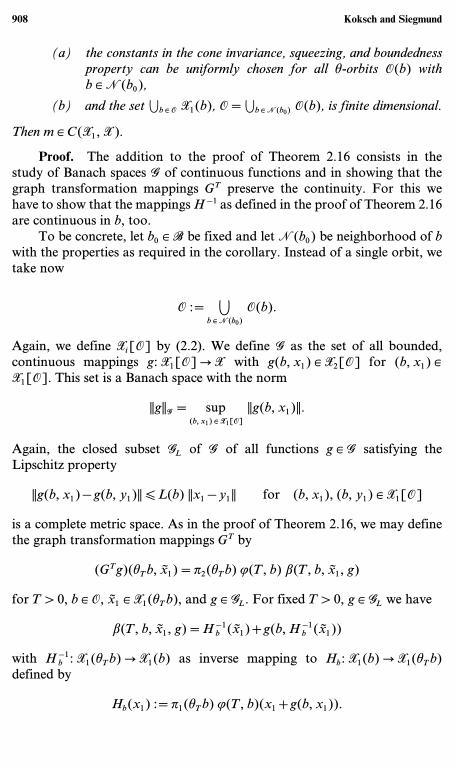
Fig. 2.1. Graph transformation mapping GT.

Moreover, let GL denote the subset of G containing all mappings whichsatisfy the global Lipschitz condition

||g(b, x1)−g(b, y1)|| [ L(b) ||x1−y1 ||

for (b, x1), (b, y1) ¥X1[O] with L from the cone invariance property. Notethat both G and GL … G are complete metric spaces. Let T > 0 be arbitrary,but fixed. We wish to define the graph transformation mapping GT: GL Q G

such that

graph((GTg)(hTb, · ))=j(T, b) graph(g(b, · ))

(see Fig. 2.1) and this means that x ¥ graph((GTg)(hTb, · )) equals j(T, b) xfor some x ¥ graph(g(b, · )). More precisely, for an x1 ¥X1(hTb) we want todefine (GTg)(hTb, x1)=x2 ¥X2(hTb) by determining an x ¥ graph(g(b, · ))such that

p1(hTb) j(T, b) x=x1 and p2(hTb) j(T, b) x=: (GTg)(hTb, x1).

To this end we show that for each T > 0, b ¥ O, X1 ¥X1(hTb), g ¥ GL, theboundary value problem

x ¥ graph(g(b, · )), p1(hTb) j(T, b) x=x1 (2.3)

has a unique solution x=b(T, b, x1, g).Uniqueness of a solution of (2.3). Assume there exist x and y with

x, y ¥ graph(g(b, · )), p1(hTb) j(T, b) x=p1(hTb) j(T, b) y=x1.


We get x−y ¥ CL(b) and the squeezing property (with xŒ=x) implies theidentity

j(t, b) x=j(t, b) y for t ¥ [0, T].

Hence x=y and there is at most one solution x=b(T, b, x1, g) of (2.3).Existence of a solution of (2.3). Let T > 0, b ¥ O, g ¥ GL be fixed and

define H: X1(b)QX1(hTb) by

H(x1) :=p1(hTb) j(T, b)(x1+g(b, x1)).

By the continuity of j(T, b) and g(b, · ), H is continuous. For x1 ¥HX1(b) …X1(hTb), any x1 in the preimage H−1(x1)={x1 ¥X1(b) : H(x1)=x1} gives rise to a solution x=x1+g(b, x1) of the boundary valueproblem (2.3). As we have already seen, there exists at most one solutiondenoted by b(T, b, x1, g) and therefore the inverse H−1 of H is given by

H−1(x1)=p1(b) b(T, b, x1, g) on HX1(hTb).

Now we show the continuity of H−1: HX1(b)QX1(b). Suppose, there is at. ¥HX1(b) …X1(hTb) such that H−1 is not continuous at t.. Then thereare e > 0 and a sequence (tk)k ¥N in X1(hTb) such that tk Q t. as kQ.and

||tk−t. || \ e for all k ¥N (2.4)

where tk :=p1(b) b(T, b, tk, g) for k ¥N 2 {.}.First, we suppose that there is a subsequence of (tk)k ¥N, denoted for

brevity again by (tk)k ¥N, with ||tk ||Q. as kQ.. Then the coercivityproperty of j implies

||tk ||=||H(tk)||=||p1(hTb) j(T, b)(tk+g(b, tk))||Q. as kQ.,

but this contradicts tk Q t..Therefore we have proved that (tk)k ¥N is bounded. Since X1(b) is a

finite-dimensional space, there is a convergent subsequence, denoted forbrevity again by (tk)k ¥N, with a limit

t.= limkQ.

tk ¥X1(b). (2.5)

By the continuity of H, we have H(tk)QH(t.). Since also H(tk)=tk Q t.=H(t.) we get t.=t. in contradiction to (2.4) and (2.5). There-fore, H and H−1 are continuous.


Now we show that H is onto, i.e., satisfies

HX1(b)=X1(hTb). (2.6)

By the coercivity of j, we have the norm coercivity ||H(t)||Q. for||t||Q. of H. Since X1(b) is finite-dimensional, H is a sequentiallycompact mapping. By [Rhe69, Theorem 3.7], H is a homeomorphismfrom X1(b) onto X1(hTb) and hence we have (2.6).

Thus we have unique solvability of (2.3), and we can define the graphtransformation mapping GT by

(GTg)(hTb, x1)=p2(hTb) j(T, b) b(T, b, x1, g)

for T > 0, b ¥ O, x1 ¥X1(hTb), and g ¥ GL. Note that we have

graph((GTg)(hTb, · ))=j(T, b) graph(g(b, · )).

Since H−1, g(b, · ) and xW p1(b) j(T, b) x are continuous, and

b(T, b, x1, g)=H−1(x1)+g(b, H−1(x1))

holds, the mapping (GTg)(hTb, · ) is also continuous.It remains to show that

||GTg||G <..

Since g ¥ G, there is an M1 with ||p2(b) x|| [M1 for all b ¥ O and all x ¥graph(g(b, · )). By the boundedness property of j there is an M2=M2(O, M1) with ||p2(hTb) j(t, b) x|| [M2 for all b ¥ O and all x ¥X with||p2(b) x|| [M1. Let b ¥ O, x1 ¥X1(hTb) be arbitrary. Then b(T, b, x1, g) ¥graph(g(b, · )), hence ||p2(b) b(T, b, x1, g)|| [M1, and therefore

||(GTg)(hTb, x1)||=||p2(hTb) j(T, b) b(T, b, x1, g)|| [M2

proving that ||GTg||G <., i.e., GTg ¥ G.

Step 2: Unique Fixed-Point of Graph Transformation Mappings. LetT > 0, b ¥ O, x1, x2 ¥X1(hTb), g ¥ GL be arbitrary. Since b(T, b, x1, g),b(T, b, x2, g) ¥ graph(g(b, · )), we get

b(T, b, x1, g)−b(T, b, x2, g) ¥ CL(b)


and the cone invariance property implies for T \ T0 a Lipschitz estimatefor GTg,

||(GTg)(hTb, x1)−(GTg)(hTb, x2)||

[ L(hTb) ||p1(hTb)(j(T, b) b(T, b, x1, g)−j(T, b) b(T, b, x2, g))||

=L(hTb) ||x1−x2 ||,

i.e., GT maps GL into G for every T \ 0, and it is a self-mapping forT \ T0. Now let T \ 0, b ¥ O, x1 ¥X1(hTb), g, h ¥ G, and x ¥ graph(g(b, · )),y ¥ graph(h(b, · )) with

p(hTb) j(T, b) x=p1(hTb) j(T, b) y=x1.

Define

xŒ :=p1(b) x+h(b, p1(b) x).

Then xŒ−y ¥ CL, and the squeezing property implies

||p2(hTb)[j(T, b) x−j(T, b) y]|| [K2e−gT ||g(b, p1(b) x)−h(b, p1(b) x)||

for T \ 0. Thus

||(GTg)(hTb, x1)−(GTh)(hTb, x1)||

[K2e−gT ||g(b, p1(b) b(T, b, x1, g))−h(b, p1(b) b(T, b, x1, g))||,

and passing to the sup over all (hTb, x1) ¥X1[O] we get

||GTg−GTh||G [ o(T) ||g−h||G

for all T > 0, g, h ¥ GL, where

o(T) :=K2e−gT.

Since g > 0, there is a positive T1 \ T0 with o(T) < 1 for T \ T1. Thus, forT \ T1, GT is a contractive self-mapping on the complete metric space GL.Now choose and fix an arbitrary T \ T1 and let gg denote the unique fixed-point of G T in GL. We show that gg is the unique fixed-point of GT forevery T \ 0.

For every T \ 0 the mapping GTgg ¥ G is uniquely determined by thegraphs

graph((GTgg)(hTb, · ))=j(T, b) graph(gg(b, · )), b ¥ O.


For T \ 0 and b ¥ O we have the identity

graph((GT+Tgg)(hT+Tb, · ))=j(T+T, b) graph(gg(b, · ))

=j(T, hTb) j(T, b) graph(gg(b, · ))

=j(T, hTb) graph(gg(hTb, · ))

=graph((GTgg)(hT+Tb, · ))

and therefore GTgg=GT+Tgg ¥ GL. Hence the composition GTGTŒgg makessense for T, TŒ \ 0 and we get

graph((GTGTŒgg)(hT+TŒb, · ))=j(T, hTŒb) graph(GTŒgg(hTŒb, · ))

=j(T, hTŒb) j(TŒ, b) graph(gg(b, · ))

=j(T+TŒ, b) graph(gg(b, · ))

=graph((GT+TŒgg)(hT+TŒb, · ))

and therefore GTGTŒgg=GTŒGTgg=GT+TŒgg for T, TŒ \ 0. We get

G T(GTgg)=GT(G Tgg)=GTgg.

Thus GTgg equals the unique fixed-point gg of G T and we have

GTgg=gg for T \ 0.

To prove the uniqueness of the fixed-point gg of GT, assume that hg isanother fixed-point. But then gg and hg are both fixed-points of GkT forevery k ¥N. Choosing k large enough such that kT \ T1 we know that GkT

has a unique fixed-point and this implies gg=hg. Note that gg depends onthe orbit O ¥O(B). Hence we rename it to gO.

Let m: X1 QX defined by

m(b, x) :=gO(b, x) for O ¥O(B), b ¥ O, x ¥X1(b).

By the uniqueness of the fixed-points gO, we have the invariance property

j(t, b) graph(m(b, · ))=graph(m(htb, · )) for t \ 0 and b ¥B,

and we may define M(b) :=graph(m(b, · )) for b ¥B. Note that gO ¥ GLimplies that for each O ¥O(B) there is a K=K(O) such that

||m(b, x)|| [K (2.7)

for b ¥ O, x ¥X1(b).


Step 3: Existence of Asymptotic Phase. Let O ¥O(B), b ¥ O andx ¥X be arbitrary and let (tk)k ¥N be a monotonically increasing sequenceof positive real numbers tk with tk Q. for kQ.. Define yŒ :=p1(b) x+m(b, p1(b) x) ¥ graph(m(b, · )) and

xk :=b(tk, b, p1(htkb) j(tk, b) x, m) ¥ graph(m(b, · )).

We get yŒ−xk ¥ CL(b) and the squeezing property implies for i=1, 2,t ¥ [0, tk]

||pi(htb)[j(t, b) x−j(t, b) xk]|| [Kie−gt ||p2(b) x−m(b, p1(b) x)||.

In particular, we find for i=1 and t=0

||p1(b) xk || [ ||p1(b) x||+||p1(b)[x−xk]||

[ ||p1(b) x||+K1 ||p2(b) x−m(b, p1(b) x)||.

Therefore we have proved that (p1(b) xk)k ¥N …X1(b) is bounded. SinceX1(b) is a finite-dimensional space, there is a convergent subsequence,denoted again by (p1(b) xk)k ¥N. Since

xk=p1(b) xk+m(b, p1(b) xk)

and m(b, · ) is continuous, also (xk)k ¥N is converging to some

xŒ ¥ graph(m(b, · )).

Then we get for i=1, 2

||pi(htb)[j(t, b) x−j(t, b) xŒ]||

[ ||pi(htb)[j(t, b) x−j(t, b) xk]||+||pi(htb)[j(t, b) xk−j(t, b) xŒ]||

[Kie−gt ||p2(b) x−m(b, p1(b) x)||+||pi(htb)[j(t, b) xk−j(t, b) xŒ]||

for all T > 0, t ¥ [0, T] and all k ¥N > 0 with tk \ T. By the continuity ofj(t, b), and because of xk Q xŒ, the second term can be made arbitrarysmall for each fixed t ¥ [0, T] choosing k large enough. Therefore,

||pi(htb)[j(t, b) x−j(t, b) xŒ]|| [Kie−gt ||p2(b) x−m(b, p1(b) x)||

for t \ 0, i.e., xŒ ¥M(b) is an asymptotic phase of x.


Step 4: Pullback Attractivity. Note that with p1 also the complemen-tary projector p2 is tempered from above. Since j(t, b) xŒ ¥M(htb) forevery x ¥X, t \ 0, b ¥B, Step 3 implies

d(j(t, b) x,M(htb)) [K0e−gt ||p2(b)[x−xŒ]|| for t \ 0

with xŒ=p1(b) x+m(b, p1(b) x) and a constant K0=K0(K1, K2) > 0. Letz ¥M(b) be arbitrary. Then, because of z−xŒ ¥ CL(b) and p1(b) x=p1(b) xŒ,

||p2(b)[x−xŒ]|| [ ||p2(b)[x−z]||+||p2(b)[z−xŒ]||

[ ||p2(b)[x−z]||+L(b) ||p1(b)[z−xŒ]||

[ (||p2(b)||+L(b) ||p1(b)||) ||x−z||.

Hence

||p2(b)[x−xŒ]|| [ (||p2(b)||+L(b) ||p1(b)||) d(x,M(b)).

Replacing b by h−tb and using the temperedness (Corollary 2.8) to choose aT=T(b) > 0 such that

K0 · (||p2(h−tb)||+L(b) ||p1(h−tb)||) [ eg

2 t for t \ T,

we obtain

d(j(t, h−tb) x,M(b)) [ e−g

2 t d(x,M(h−tb)) [ e−g

2 t d(D |M(h−tb)) (2.8)

for t \ T with T independent of D. Moreover, if supb ¥B ||p1(b)|| <. andsupb ¥BL(b) <. then T can be chosen independently of b. To finish theproof we use the fact that y ¥M implies d(D |M) [ d(D | {y}), the esti-mate (2.7), the inclusion 0 ¥X(h−tb) and the boundedness of D to obtain

d(D |M(h−tb)) [ d(D | {m(h−tb, 0)}) [ |D|+K,

proving the exponential pullback attractivity of M. i

The following corollary describes a situation, where the manifold iscontinuous.

Corollary 2.17. Let the NDS j satisfy the assumptions ofTheorem 2.16. Further we assume:

(1) B is a metric space, j ¥ C(R \ 0×B×X, X) and h ¥ C(R×B, B).(2) (b, x)W p1(b) x is continuous on B×X.(3) For each b0 ¥B there is an open neighborhoodN(b0) such that


(a) the constants in the cone invariance, squeezing, and boundednessproperty can be uniformly chosen for all h-orbits O(b) withb ¥N(b0),

(b) and the set 1b ¥ O X1(b), O=1b ¥N(b0) O(b), is finite dimensional.

Then m ¥ C(X1, X).

Proof. The addition to the proof of Theorem 2.16 consists in thestudy of Banach spaces G of continuous functions and in showing that thegraph transformation mappings GT preserve the continuity. For this wehave to show that the mappingsH−1 as defined in the proof of Theorem 2.16are continuous in b, too.

To be concrete, let b0 ¥B be fixed and let N(b0) be neighborhood of bwith the properties as required in the corollary. Instead of a single orbit, wetake now

O := 0b ¥N(b0)

O(b).

Again, we define Xi[O] by (2.2). We define G as the set of all bounded,continuous mappings g: X1[O]QX with g(b, x1) ¥X2[O] for (b, x1) ¥X1[O]. This set is a Banach space with the norm

||g||G= sup(b, x1) ¥X1[O]

||g(b, x1)||.

Again, the closed subset GL of G of all functions g ¥ G satisfying theLipschitz property

||g(b, x1)−g(b, y1)|| [ L(b) ||x1−y1 || for (b, x1), (b, y1) ¥X1[O]

is a complete metric space. As in the proof of Theorem 2.16, we may definethe graph transformation mappings GT by

(GTg)(hTb, x1)=p2(hTb) j(T, b) b(T, b, x1, g)

for T > 0, b ¥ O, x1 ¥X1(hTb), and g ¥ GL. For fixed T > 0, g ¥ GL we have

b(T, b, x1, g)=H−1b (x1)+g(b, H

−1b (x1))

with H−1b : X1(hTb)QX1(b) as inverse mapping to Hb: X1(b)QX1(hTb)defined by

Hb(x1) :=p1(hTb) j(T, b)(x1+g(b, x1)).


By the continuity of g, p1, j and h−T, the required continuity ofGTg: X1[O]QX follows now from the continuity of (b, x1)WH

−1h−Tb(x1) as

a mapping from X1[O] into X. The proof of the latter one can be donesimilar to the corresponding part in the proof of Theorem 2.16, where wenow have to consider sequences in X1[O]. i

2.3. Pullback Attractors for Nonautonomous Dynamical Systems

The following theorem shows that we can easily construct a globalpullback attractor once we have a compact, forward invariant, globallypullback absorbing set.

Theorem 2.18 [Sch92, CF94, FS96, Sch99]. Suppose that A is acompact, forward invariant, globally pullback absorbing set. ThenA,

A(b) :=3t \ 0

j(t, h−tb) A(h−tb) for b ¥B,

is a global pullback attractor.

Proof. Since A is forward invariant, A(b) is the intersection of adecreasing sequence of compact sets contained in A, hence is non-void andcompact, moreover

limtQ.d(j(t, h−tb) A(h−tb) |A(b))=0. (2.9)

Using the elementary fact that if (Dn) is a decreasing sequence of compactsets and f is continuous then 4n f(Dn)=f(4n Dn), the cocycle propertyand the monotonicity of j(t, h−tb) A(h−tb) we obtain for any T ¥ R \ 0

j(T, b)A(b)=3t \ 0

j(T, b) j(t, h−tb) A(h−tb)

=3t \ 0

j(T+t, h−t−T(hTb)) A(h−t−T(hTb))

=3t \ T

j(T, h−t(hTb)) A(h−t(hTb))

=3t \ 0

j(T, h−t(hTb)) A(h−t(hTb))=A(hTb),

proving the invariance of A.


To see that A is globally pullback attracting choose a bounded setD …X, b ¥B and an e > 0. Due to formula (2.9) there exists a T0=T0(e, D, b) \ 0 such that

d(j(T0, h−T0b) A(h−T0b) |A(b)) < e,

and since A is absorbing, there exists a T1=T1(h−T0b, D) \ 0 with

j(t−T0, h−(t−T0)(h−T0b)) D … A(h−T0b) if t−T0 \ T1.

Applying j(T0, h−T0b) to this inclusion, the cocycle property implies

j(t, h−tb) D … j(T0, h−T0b) A(h−T0b).

Using the fact that if D1 …D2 then d(D1 |A) [ d(D2 |A), we obtain

d(j(t, h−tb) D |A(b)) < e for t \ T0+T1,

proving that A is globally pullback attracting. i

The next lemma shows that we only need the existence of an absorbingset A, if we have a suitable smoothing property of j. This smoothingproperty is expressed by the assumption that the set Ac is compact for suf-ficiently large c \ 0. A similar property is used in [Tem97] for semiflows,and it is called there uniform compactness property.

Lemma 2.19. Suppose that A is a globally pullback absorbing set.Then A0,

A0(b) :=0s \ 0

j(s, h−sb) A(h−sb) for b ¥B,

is globally pullback absorbing and forward invariant. If there is a c \ 0 suchthat Ac,

Ac(b) :=cl(j(c, h−cb) A0(b)) for b ¥B,

is compact, then Ac is a compact, forward invariant, globally pullbackabsorbing set.

Proof. For y \ 0 let

Ay(b) :=0s \ y

j(s, h−sb) A(h−sb) for b ¥B.


Let b ¥B, t \ 0. Then

j(t, b) Ay(b)=0s \ y

j(t+s, h−sb) A(h−sb)

= 0r \ y+t

j(r, h−rhtb) A(h−rhtb)

ı 0r \ y

j(r, h−rhtb) A(h−rhtb)

=Ay(htb).

Thus Ay is forward invariant for each y \ 0.Since A is globally pullback attracting, for any b ¥B and any

bounded set D there is a T(b,D) with j(t, h−tb) D ı A(b) for t \ T(b,D).Since j(y, h−yb) A(h−yb) ı Ay(b) and

j(t, h−th−yb) D ı A(h−yb) for t \ T(h−yb, D)

we have

j(t, h−tb) D ı Ay(b) for t \ y+T(h−yb, D).

Thus Ay is pullback attracting for each y \ 0. For y=0 we obtain the firstclaim.

Now assume that there exists a c \ 0 such that Ac is compact. Sincej(c, h−cb) A0=Ac(b), the set Ac is the closure of the forward invariant,globally pullback attracting set Ac(b) and hence it is forward invariant,globally pullback attracting, too. i

Obviously, if A is compact, positively invariant and globally pullbackattracting then we may choose c=0 and hence A0=A.

In Theorem 2.16 we proved the existence of an inertial manifold whichis exponentially attracting in the sense of forward convergence, i.e.,j(t, b) x is converging to its asymptotic phase j(t, b) xŒ. Moreover, weproved that the inertial manifold is globally pullback attracting if theprojector p1 is tempered from above.

Combining the Theorems 2.16 and 2.18, we give a sufficient conditionfor the existence of a global pullback attractor which is contained in theinertial manifold.

Corollary 2.20. Let the assumptions of Theorem 2.16 be satisfied witha projector p1 which is tempered from above. Moreover, suppose that A is acompact, forward invariant, globally pullback absorbing set which is tempered


from above, i.e., the function bW |A(b))| is tempered from above, where|D| :=sup{||x|| : x ¥D}. Then the global pullback attractorA,

A(b)=3t \ 0

j(t, h−tb) A(h−tb) b ¥B,

is contained in the inertial manifoldM.

Proof. By Theorem 2.16 we have the existence of the globallypullback attracting inertial manifold M satisfying (2.8).

Let A be a compact, forward invariant, globally pullback absorbingset which is tempered from above. Theorem 2.18 implies the existence ofthe global pullback attractor A which is also tempered from above. Usingthe invariance of A, the estimate (2.7) and choosing a TŒ > T such that|A(h−tb)| [ e

g

4 t for t \ TŒ (Corollary 2.8), we get from (2.8) for t \ TŒ

d(A(b) |M(b))=d(j(t, h−tb)A(h−tb) |M(b))

[ e−g

2 t d(A(h−tb) |M(h−tb))

[ e−g

2 t d(A(h−tb) | {m(h−tb, 0)})

[ e−g

2 t(eg

4 t+K).

Since this expression tends to 0 for tQ., we obtain d(A(b) |M(b))=0and conclude that A(b) …M(b) for all b ¥B. i

3. NONAUTONOMOUS EVOLUTION EQUATIONS

3.1. Processes

Let (X, || · ||X) be a Banach space. The solutions of a nonautonomousevolution equation will not generate a semi-flow but a so-called process(Dafermos [Daf71]) (or two-parameter semi-flow).

Definition 3.1 (Process). A process m on X is a continuous mapping

{(t, s, x) ¥ R×R×X : t \ s} ¦ (t, s, x)W m(t, s, x) ¥X

which satisfies

(i) m(s, s, · )=idX for s ¥ R;

(ii) the process property for t \ y \ s, x ¥X, i.e.,

m(t, y, m(y, s, x))=m(t, s, x).


The next lemma explains how a process defines an NDS. For a morerefined construction associating, e.g., to a compact process an NDS withcompact base see Dafermos [Daf75] for details.

Lemma 3.2 (Process defines NDS). Suppose that m is a process. Thenj: R \ 0×B×XQX,

j(t, b) x=m(t+b, b, x) (3.1)

is an NDS with base B=R and driving system h: R×BQB,

h(t) b=t+b.

Moreover, for t \ s and x ¥X the relation m(t, s, x)=j(t−s, s) x holds.

Proof. h is a dynamical system. We have

j(0, b)=m(b, b, · )=idX.

We use the process property of m to obtain for t, s \ 0, b ¥B

j(t+s, b)=m(t+s+b, b, · )

=m(t+s+b, s+b, m(s+b, b, · ))

=j(t, hsb) p j(s, b),

proving the cocycle property of j. The continuity of m implies the continu-ity of (t, x)W j(t, b) x. Now substitute t by t−s and b by s in (3.1) to seethat m(t, s, x)=j(t−s, s) x. i

Theorem 3.3 (Inertial Manifold for Processes). Suppose that m isa process on X and let (pi(y))y ¥ R … L(X), i=1, 2, be two families ofcomplementary projectors p1(y) and p2(y). Let m satisfy the

• cone invariance property, i.e., there are L: RQ R > 0 and T0 \ 0 suchthat for y ¥ R and x, y ¥X,

x−y ¥ CL(y) :={t : ||p2(y) t||X [ L(y) ||p1(y) t||X}

implies

m(t, y, x)−m(t, y, y) ¥ CL(t) for t \ y+T0;


• squeezing property, i.e., there exist positive constants K1, K2 and g

such that for every y ¥ R, x, y ¥X and T > 0 the identity

p1(y+T) m(y+T, y, x)=p1(y+T) m(y+T, y, y)

implies for all xŒ ¥X with p1(y) xŒ=p1(y) x and xŒ−y ¥ CL(y) theestimates

||pi(t)[m(t, y, x)−m(t, y, y)]||X [Kie−g(t−y) ||p2(y)[x−xŒ]||X, i=1, 2,

for t ¥ [y, y+T];

• boundedness property, i.e., for all t \ 0 and allM1 \ 0 there exists anM2 \ 0 such that for y ¥ R, x ¥X with ||p2(y) x||X [M1 the estimate

||p2(t) m(t+y, y, x)||X [M2

holds.

• coercivity property, i.e., for all t, y ¥ R with t \ y and allM3 \ 0 thereexists an M4 \ 0 such that for x ¥X with ||p1(y) x||X \M4 theestimate

||p1(t) m(t, y, x)||X \M3

holds.Then there exists an inertial manifold M=(M(y))y ¥ R of m with

the following properties:

(i) M(y) is a graph in p1(y) X À p2(y) X,

M(y)={x1+m(y, x1) : x1 ¥ p1(y) X}

with a mapping m(y, · )=m(y): p1(y) XQ p2(y) X which isglobally Lipschitz continuous

||m(y, x1)−m(y, y1)||X [ L(y) ||x1−y1 ||X.

(ii) M is exponentially attracting, more precisely

||pi(t)[m(t, y, x)−m(t, y, xŒ)]||X

[Kie−g(t− y) ||p2(y) x−m(y, p1(y) x)||X

for t \ y, i=1, 2, with an asymptotic phase xŒ=xŒ(y, x) ¥M(y)of x and the constants K1, K2 > 0 from the squeezing propertywhich are independent of y and x.


(iii) If in addition p1 is tempered from above, thenM is exponentiallypullback attracting, i.e., for each bounded set D …X there is aconstant K > 0 and for every y ¥ R there is a T \ y such that

d(m(t, y−t, D) |M(y)) [Ke−gt/2 for t \ T.

Proof. By Lemma 3.2, the process m defines an NDS j with baseB=R and driving system h: R×BQB with h(t) y=t+y, y=b ¥B. NowTheorem 3.3 follows from Theorem 2.16. i

3.2. Nonautonomous Evolution Equations

Let X ıY be Banach spaces equipped with norms || · ||X, || · ||Y, and let(A(t))t ¥ R be a family of densely defined linear operators A(t) on Y withdomain D(A(t)) in Y. We consider a nonautonomous evolution equation

x+A(t) x=f(t, x) (3.2)

which satisfies the following assumptions:

(A1) Linearity A(t):

• Existence of evolution operator of the linear system: Under suitableadditional assumptions on X, Y, A and f (see for example [Hen81,DKM92, Lun95]), we may define the evolution operator F : {(t, s) ¥R2: t \ s}Q L(Y, Y) of the linear equation

x+A(t) x=0 (3.3)

in Y as the solution of

ddt

F(t, s)+A(t) F(t, s)=0 for t > s, s ¥ R

and

F(y, y)=idY for y ¥ R.

• There are constants k0,..., k4 \ 1, b2 > b1, a ¥ [0, 1[, a monotoni-cally decreasing function k ¥ C(R > 0, R > 0) with k(t) [ k0t−a, and afamily p1=(p1(t))t ¥ R of linear, invariant projectors p1(t): YQY,i.e.,

p1(t) F(t, s)=F(t, s) p1(s) for t \ s,


such that F(t, s) p1(s) can be extended to a linear, bounded operatorfor t ¥ R with

ddt

F(t, s) p1(s)+A(t) F(t, s) p1(s)=0 for t, s ¥ R

and

||F(t, s) p1(s)||L(X, X) [ k1e−b1(t−s) for t [ s,

||F(t, s) p2(s)||L(X, X) [ k2e−b2(t−s) for t \ s,

||F(t, s) p1(s)||L(Y, X) [ k3e−b1(t−s) for t [ s,

||F(t, s) p2(s)||L(Y, X) [ k4k(t−s) e−b2(t−s) for t > s

(3.4)

with p2, p2(t)=idY−p1(t), as the complementary projector to p1in Y.

(A2) Nonlinearity f(t, x): The nonlinear function f ¥ C(R×X, Y) isassumed to be globally bounded and to satisfy the Lipschitz inequality

||pi(t)[f(t, x)−f(t, y)]||Y [ ci(||p1(t)[x−y]||X, ||p2(t)[x−y]||X) (3.5)

for all t ¥ R, x, y ¥X, where ci are suitable norms on R2.

(A3) Existence of Mild Solutions: We have the existence and unique-ness of the mild solutions

m( · , y, t) ¥ C([y,.[, X)

of (3.2) with initial condition x(y)=t ¥X, i.e., let m be the continuoussolution of the integral equation

x(t)=F(t, y) t+Ft

y

F(t, r) f(r, x(r)) dr for t \ y.

These are our assumptions.

Remark 3.4.

(1) Conditions like our assumptions can be found in the literatureand they are standard for ordinary differential equations and fortime-independent evolution equations in the non-selfadjoint case,see for example [Tem97]. For concrete examples of the realiza-tion of these assumptions we refer to Section 4, where we will


apply our following Theorem 3.10 on the existence of inertialmanifolds in these special situations.

(2) At least in special cases like X=Y, it is possible to allow time-depending Lipschitz constants L and to use exponential dicho-tomy conditions with time-depending rates b1, b2, i.e., to replacekjebi(t−s) by kje >ts bi(r) dr in (3.4). For reason of simplicity and inorder to avoid technical complications, in this paper we onlyconsider the case where L and b1, b2 are time-independent.

3.3. Comparison Theorems

In order to apply Theorem 3.3, we have to show the cone invarianceproperty and the squeezing property for the process m with respect to theprojector p1.

For fixed r1, r2 \ 0 and T \ 0, we define

(L1w)(t) :=k3 FT

te−b1(t−r)1 c1(w(r)) dr,

(L2w)(t) :=k4 Ft

0k(t−r) e−b2(t−r)c2(w(r)) dr+k2e−b2tLw1(0)

and

q(t) :=(k1e−b1(t−T)r1, k2e−b2tr2)

for t ¥ [0, T] and w ¥ C([0, T], R2). Then q ¥ C([0, T], R2\ 0). Because ofk(t) [ k0t−a with a ¥ [0, 1[, L is an at most weakly singular integral opera-tor from C([0, T], R2) into C([0, T], R2). Moreover, L is completelycontinuous.

Lemma 3.5. Assume there are L > 0 and T0 \ 0 such that for eachT \ T0 the inequality

v2(T) [ Lr1 (3.6)

holds for each solution v ¥ C([0, T], R2\ 0) of

v i(t) [ (Lv) i (t)+q i(t) for i=1, 2, t ¥ [0, T] (3.7)

with r1 \ 0, r2=0. Then m possesses the cone invariance property withrespect to p with the parameters L > 0 and T0 \ 0.


Proof. The cone invariance property is shown if

||p2(t)[m(t, y, x)−m(t, y, y)]||X [ L ||p1(t)[m(t, y, x)−m(t, y, y)]||X(3.8)

for each y ¥ R, t \ y+T0 and x, y ¥X with

||p2(y)[x−y]||X [ L ||p1(y)[x−y]||X. (3.9)

Let y ¥ R, T > 0 and x, y ¥X with (3.9) be fixed and let

l(t) :=m(t, y, x)−m(t, y, y), fD(t) :=f(t, m(t, y, x))−f(t, m(t, y, y))

on [y, y+T]. Then we have

p1(t) l(t)=F(t, y+T) p1(y+T) l(y+T)+Ft

y+TF(t, r) p1(r) fD(r) dr

and

p2(t) l(t)=F(t, y) p2(y)[x−y]+Ft

y

F(t, r) p2(r) fD(r) dr

on [y, y+T]. Let v: [0, T]Q R2\ 0 be defined by

v(t)=(||p1(y+t) l(y+t)||X, ||p2(y+t) l(y+t)||X). (3.10)

Then

v1(t) [ ||F(y+t, y+T) p1(y+T) l(y+T)||X

+FT

t||F(y+t, y+r) p1(y+r) fD(y+r)||X dr

[ ||F(y+t, y+T) p1(y+T)||L(X, X) ||p1(y+T) l(y+T)||X

+FT

t||F(y+t, y+r) p1(y+r)||L(Y, X) ||p1(y+r) fD(y+r)||Y dr

and

v2(t) [ ||F(y+t, y) p2(y) l(y)||X

+Ft

0||F(y+t, y+r) p2(y+r) fD(y+r)||X dr

[ ||F(y+t, y) p2(y)||L(X, X) ||p2(y) l(y)||X

+Ft

0||F(y+t, y+r) p2(y+r)||L(Y, X) ||p2(y+r) fD(y+r)||Y dr.


The exponential dichotomy and Lipschitz assumptions (3.4), (3.5) andinequality (3.9) imply that the function v defined by (3.10) satisfies (3.7)with

r1 :=||p1(y+T)[m(y+T, y, x)−m(y+T, y, y)]||X, r2 :=0.

By the assumptions we have (3.9), i.e., (3.8) holds. i

Lemma 3.6. Assume there are positive numbers L, g, K1, K2 such that

v i(t) [Kie−gtr2 for t ¥ [0, T] (3.11)

holds for each T > 0 and each solution v ¥ C([0, T], R2\ 0) of (3.7) withr1=0, r2 \ 0. Then m possesses the squeezing property with respect to p withthe parameters L, g, K1, K2.

Proof. The squeezing property is shown if we find g > 0 and con-stants K1, K2 > 0 such that for all y ¥ R, x, y ¥X and T > 0 the identity

p1(y+T) m(y+T, y, x)=p1(y+T) m(y+T, y, y) (3.12)

implies for all xŒ ¥X with

p1(y) xŒ=p1(y) x and ||p2(y)[xŒ−y]||X [ L ||p1(y)[xŒ−y]||X(3.13)

the estimates

||pi(t)[m(t, y, x)−m(t, y, y)]||X [Kie−g(t− y) ||p2(y)[x−xŒ]||X (3.14)

for i=1, 2 and t ¥ [y, y+T].As in the proof of Lemma 3.5 let y ¥ R, T > 0 and x, y, xŒ ¥X with

(3.12), (3.13) be fixed and let

l(t) :=m(t, y, x)−m(t, y, y), fD(t) :=f(t, m(t, y, x))−f(t, m(t, y, y))

on [y, y+T]. Then we have

p1(t) l(t)=F(t, y+T) p1(y+T) l(y+T)+Ft


=Ft



and

p2(t) l(t)=F(t, y) p2(y)[xŒ−y]+F(t, y) p2(y)[x−xŒ]

+Ft

y

F(t, r) p2(r) fD(r) dr

on [y, y+T]. Similar to the proof of Lemma 3.5, the exponential dicho-tomy and Lipschitz assumptions (3.4), (3.5) and inequality (3.13) imply thatthe function v: [0, T]Q R2\ 0 defined by (3.10) satisfies (3.7) with

r1 :=0, r2 :=||p2(y)[xŒ−x]||X.

By assumption we have (3.11), i.e., (3.14) holds. i

To estimate the solutions v of (3.7), we make an excursion to thetheory of monotone iterations in ordered Banach spaces, see for example[KLS89]. Note that similar ideas are used in [AC98].

Let B be a Banach space and let C be an order cone in B. The ordercone C induces a semi-order [C in B by

u [C w :Z w−u ¥ C.

The norm in B is called semi-monotone if there is a constant c with||x||B [ c||y||B for each x, y ¥B with 0 [C x [C y. The cone C is callednormal if the norm in B is semi-monotone, and C is called solid if C

contains an open ball with positive radius.Note that C([0, T], RN\ 0) is a normal, solid cone in C([0, T], RN).In a Banach space B with normal and solid cone C, we study the

fixed-point problem

u=Pu+p (3.15)

with p ¥B and P: BQB. We assume that P is completely continuous,increasing,

Pu [C Pv if u [C v,

subadditive,

P(u+v) [C Pu+Pv, u, v ¥ C,

and homogeneous with respect to nonnegative factors,

P(lu)=lPu l ¥ R \ 0, u ¥ C.


Definition 3.7. A function w ¥B is called upper (lower) solution of(3.15) if Pw+p [C w (w [C Pw+p).

Our goal is to ensure the existence of a unique solution w ¥ C of (3.15)and to estimate lower solutions v ¥ C of (3.15) by solutions or uppersolutions of (3.15).

For x, y ¥B with x [C y, we denote by

[x, y]C :={z ¥B : x [C z [C [ y}

the order interval given by x and y.

Lemma 3.8. Let x¯ 0

¥ C and x0 ¥ C be a lower and an upper solution of(3.15) with x

¯ 0[C [ x0. Then the sequences (x¯ n

)n ¥N and (xn)n ¥N with x¯ n+1=

Px¯ n+p and xn+1=Pxn+p converges to solutions x¯ g and xg of (3.15) and

x¯ 0

[C x¯ g [C xg [C x0. (3.16)

Proof. We follow the proof of Theorem 3.1 in [EL75]. i

By the normality of the cone, there is a constant c > 0 such that||w1 ||B [ c||w2 ||B for all w1, w2 ¥ C satisfying w1 [C w2. Hence, the sets[x¯ 0, x0]C ı [0, x0]C are norm bounded by c ||x0 ||B and closed. Because of

the complete continuity of P, there is a convergent subsequence (x¯ nk)k ¥N of

(x¯ n)n ¥N in [x

¯ 0, x0]C with limit x

¯ g ¥ [x¯ 0, x0]C. Suppose (x

¯ n)n ¥N is not con-

vergent to x¯ g. Then there are d > 0 and a subsequence (x

¯ mk)k ¥N of (x

¯ n)n ¥N

satisfying

||x¯ mk−x¯ g ||B > d, x

¯ mk[C x¯ g, x

¯ nk[C x¯ mk

for k ¥N.

By the normality of the cone, we have

||x¯ g−x¯ mk

||B [C c||x¯ g−x¯ nk||B Q 0

for kQ. and a contradiction is reached. Thus, (x¯ n)n ¥N is convergent

to x¯ g.

Analogously, one can show the converges of (xn)n ¥N.By construction we have

x¯ 0

[C x¯ 1[C x¯ 2

[C · · · [C x¯ g [C xg [C · · · [C x2 [C x1 [C x0.

The inequalities x¯ n

[C x¯ n+1=Px¯ n+p [C x¯ g, the convergence x

¯ nQ x¯ g and

the continuity of P imply

x¯[C Px¯ g+p [C x¯ g,

i.e., x¯ g is a solution of (3.15).


Similarly follows that xg is a solution of (3.15), too. By constructionwe have (3.16). i

Lemma 3.9. Assume that there are y ¥ int C and d ¥ [0, 1[ with

Py [C dy.

Then there is a unique solution xg of (3.15) in C and

x¯[C xg [C x (3.17)

holds for each lower solution x¯¥ C and each upper solution x ¥ C of (3.15).

Proof. First we note that by the normality and solidity of C, for eachx ¥ C there is ||x||y defined by

||x||y :=inf{m \ 0 :−my [C x [C my}.

Now we show that 0 is the unique solution of

x=Px (3.18)

in C. Since P is subadditive, we have P0=P(0+0) [C P0+P0 and hence0 [C P0. From 0 [C y follows 0 [ P0 [C Py [C dy, i.e., 0 [C P0 [C dy.Thus 0 [C P0 [C dny for all n ¥N. Hence 0=P0. Let x ¥ C be a solution of(3.18). Then 0 [C x [C m(x) y. By the monotony and homogeneity of P wehave 0 [C x [C ||x||y dny for all n ¥N and hence x=0. Therefore, 0 is theunique solution of (3.18) in C.

By the subadditivity of P and because of p ¥ C, 0 is a lower solution of(3.15). Moreover ly with l \

||q||y1−d is an upper solution of (3.15). By Lem-

ma 3.8, the existence of at least one solution x1 ¥ C of (3.15) follows.Assume there is another solution x2 ¥ C of (3.15). By Lemma 3.8, we

find a solution x3 ¥ C of (3.15) with 0 [C xi [C [ x3 [C ly for i=1, 2 withl \ max{||x1 ||y, ||x2 ||y,

||q||y1−d }. Hence, without loss of generality we may assume

that 0 [C x1 [C [ x2 and x1 ] x2.Let w :=x2−x1. Then 0 [C w, w ] 0, and, by the subadditivity of P,

w=Px2−Px1=P(x1+w)−Px1 [C Px1+Pw−Px1=Pw.

Thus, w is a lower solution of (3.18). Since m(w) y is an upper solution of(3.18) and w [C ||w||y y, Lemma 3.8 with p=0 implies the existence of asolution v ¥ [w, y]C of (3.18). As above shown, v=0 is the unique solutionof (3.18) in C. Hence w=0 in contrast to the assumption x1 ] x2. Thus(3.15) possesses a unique solution xg ¥ C.


Now let x¯¥ C, x ¥ C be arbitrary lower and upper solutions of (3.15).

By Lemma 3.8 and by the uniqueness of the solution xg of (3.15), we havex¯[C xg [C ly with l \ max{||x

¯||y, ||xg ||y,

||q||y1−d }. On the other hand, with the

lower solution 0 of (3.15), we have 0 [C xg [C x. Thus (3.17) holds. i

In order to apply Lemma 3.9 to our situation, we choose B=C([0, T], R2) and C=C([0, T], R2\ 0). Then C is a normal cone. Theoperator P=L is increasing and completely continuous, and p=q belongsto C. So we only have to find a function w* in the interior of C with

Lw* [C ew* with some e ¥ [0, 1[. (3.19)

Further we can estimate the solutions v of (3.7) by solutions w ¥ C of

Lw+q [C w. (3.20)

3.4. Inertial Manifold Theorem for Nonautonomous Evolution Equations

Now we are in a position to prove the following theorem.

Theorem 3.10 (Inertial Manifolds for Nonautonomous Evolution Equa-tions). Under the general assumptions in Section 3.2, let tg \ 0 be fixedwith

kg :=limtQ t

*

k(t) <., k(t) > kg for t < tg. (3.21)

Further let

k5 \ d Ft*

0k(r) e−dr dr+kg lim

tQ t*

e−dt for all d ¥ ] 0, b2−b1[.(3.22)

Assume that there are positive numbers r1 < r2 with

G(r1)=G(r2)=0, G|[r1, r2] ] 0 (3.23)

and

k1k2r1 < k−12 kgr5 (3.24)

where G: R > 0 Q R is defined by

G(r) :=b2−b1−k3c1(1, r)−k4k5r−1c2(1, r).


Then there are positive numbers g1 < g2 with

gi=b1+k3c1(1, ri)=b2−k4k5r−1i c2(1, ri),

and the claim of Theorem 3.2 holds for the process m generated by (3.2) with

g :=g2, L ¥ ] k1r1, k−12 k

−15 kgr2[, (3.25)

and

K1 :=k2k5

r2kg−k2k5L, K2 :=r2K1. (3.26)

Remark 3.11. Because of limrQ 0 G(r)=limrQ.G(r)=−., the exis-tence of rg > 0 with G(rg) > 0 implies the existence of positive numbersr1 < r2 with (3.23). Since G(r1)=0 and r1 < rg imply

r1 <k4k5r

−1g c2(1, rg)

b2−b1−k3c1(1, rg),

the inequality (3.24) holds if

b2−b1 > k3c1(1, rg)+k1k2k4k

25

kgrgc2(1, rg). (3.27)

Since (3.27) implies G(rg) > 0, the conditions (3.23), (3.24) can be replacedby (3.27) for some rg > 0.

Proof of Theorem 3.10. We show that the process m generated by(3.2) satisfies the assumptions of Theorem 3.2. We split the proof into fiveparts: First we show that (3.23) implies the existence of solutions of (3.19)and (3.20). Then we verify the four required properties for the process m.

Step 1: Determining of Solutions of (3.19) and (3.20). In order to finda solution w* of (3.19), first we look for w ¥ C in the form

w(t)=e−gt(1, r) (3.28)

with r > 0 and satisfying

w1(t) \ (Lw)1 (t)+c1e−b1(t−T) (3.29)


and

w2(t) \ (Lw)2 (t)+(c2r−k2L) e−b2t (3.30)

for t ¥ [0, T] with suitable positive c1 and c2.If we assume g > b1 and

g \ b1+k3c1(1, r) (3.31)

then because of

egt(Lw)1 (t)=k3c1(1, r) FT

te (g−b1)(t−r) dr

=k3c1(1, r)

g−b1(1− e (g−b1)(t−T)),

we may choose

c1=c1(r, g) :=k3c1(1, r)

g−b1e−gT (3.32)

in order to satisfy (3.29). Remains to satisfy (3.30).Inserting (3.28) in (3.30) and dividing by r e−gt, we have to satisfy

1 \H(t, r, g) (3.33)

for t ¥ [0, T] where H: [0,.[×R×RQ R is defined by

H(t, r, g) :=c2(1, r)

rk4 F

t

0k(r) e−(b2 −g) r dr+c2e−(b2 −g) t.

We choose

c2=c2(r, g) :=c2(1, r)(b2−g) r

k4kg.

Because of

D1H(t, r, g)=1 −(b2−g) c2+c2(1, r)

rk4k(t)2 e−(b2 −g) t


and because of the monotonicity of k, the function H(· , r, g) is maximizedat tg. Hence we have

H(t, r, g) [H(tg, r, g)

=c2(1, r)

rk4 1F

t*

0k(r) e−(b2 −g) r dr+(b2−g)−1 kge−(b2 −g) t*2

for all t \ 0. Because of (3.22), inequality (3.33) is satisfied if

c2(1, r)r

k4k5 [ b2−g. (3.34)

Combining (3.31) with (3.34), we find

b1+k3c1(1, r) [ g [ b2−k4k5r−1c2(1, r) (3.35)

as a sufficient condition for (3.29) and (3.30).By assumption there are positive numbers r1 < r2 with (3.23) and

(3.24). Let

gi :=b1+k3c1(1, ri)=b2−k4k5r−1c2(1, ri).

Then (g1, r1) and (g2, r2) solve (3.35).Moreover, g2 > g1. To show this, we note that g2 \ g1, by the mono-

tonicity of c1. Assuming g1=g2 we find c1(1, r1)=c1(1, r2) and c2(r−11 , 1)=

c2(r−12 , 1). By the convexity of the c1 and c2-balls we had c1(1, r)=

c1(1, r1) and c2(r−1, 1)=c2(r−11 , 1) for r ¥ [r1, r2]. This would imply the

constance of G on [r1, r2] in contradiction to (3.23).Because of (3.24) we can choose

L ¥ ] k1r1, k−12 k

−15 kgr2[. (3.36)

Now we define wi ¥ C, i=1, 2, by

wi(t) :=e−git(1, ri). (3.37)

Then

w1i (t) \ (Lwi)1 (t)+

k3c1(1, r)g−b1

e−gT e−b1(t−T)

and

w2i (t) \ (Lwi)2 (t)+(rik

−15 kg−k2L) e−b2t


on [0, T] because of

c1(ri, gi)=k3c1(1, ri)

gi−b1=1, c2(ri, gi)=

c2(1, ri) k4kg

(b2−gi) ri=k−15 kg.

Because of (3.36) we have

r2k−15 kg > k2L (3.38)

and inequality (3.19) holds for w* :=w2.Let now C1 ¥ [0, 1], C2 > 0 satisfy

C2(C1e−g1T+(1−C1) e−g2T) \ k1r1,

C2(C1r1k−15 kg+(1−C1) r2k

−15 kg−k2L) \ k2r2. (3.39)

Then

w :=C2(C1w1+(1−C1) w2)

solves

Lw+q [C w,

and Lemma 3.9 implies

v [C w

for each solution v ¥ C of (3.7).

Step 2: Verification of the Cone Invariance Property. Because of(3.38) we can fix

r ¥ ] max{r1, k2k5k−1g L}, r2[.

Let r2=0 and r1 \ 0. Then (3.39) is satisfied with

C1 :=r2− r

r2−r1, C2 :=

k1r1C1e−g1T+(1−C1) e−g2T

.

Thus we find

v2(t) [ w2(t)=C2(C1w21(t)+(1−C1) w

22(t))=L(r, t) r1

for t ¥ [0, T] with

L(r, t)=k1(r2− r) r1e−g1t+(r−r1) r2e−g2t

(r2− r) e−g1T+(r−r1) e−g2T.


Especially we have

v2(T) [ L(r, T) r1.

The inequalities g2 > g1 > b1 imply

L(r, T)Q k1r1 as TQ..

Hence there are T0 \ 0 and L \ 0 with (3.6), if the additional inequality

k1r1 < L

holds, which trivially follows from (3.36).By Lemma 3.5, the cone invariance property of m as required in

Theorem 3.3 is verified.

Step 3: Verification of the Squeezing Property. Now let r1=0 andr2 \ 0. Then we may choose

C1 :=0, C2 :=k2k5r2

r2kg−k2k5L

in order to satisfy (3.39). Thus we find

v(t) [k2r2

r2kg−k2k5Le−g2t(1, r2) for t ¥ [0, T].

Hence (3.11) holds with

g :=g2, K1 :=k2k5

r2kg−k2k5L, K2 :=r2K1

and L satisfying (3.36). By Lemma 3.6, the squeezing property of m asrequired in Theorem 3.3 is verified.

Step 4: Verification of the Boundedness Property. By the boundednessof f there is a number F \ 0 with

||f(x)||Y [ F for x ¥X.

Thus, for y ¥ R, t \ y, x ¥X,

p2(t) m(t, y, x)=F(t, y) p2(y) x+Ft

y

F(t, r) p2(r) f(r, m(r, y, x)) dr


and, by the exponential dichotomy conditions (3.4),

||p2(t) m(t, y, x)||X [ ||F(t, y) p2(y)||L(X, X) ||p2(y) x||X

+Ft

y

||F(t, r) p2(r)||L(Y, X) ||f(r, m(r, y, x))||X dr

[ k2e−b2(t−y) ||p2(y) x||X+Fk4 Ft

y

k(t−r) e−b2(t−r) dr

=k2e−b2(t−y) ||p2(y) x||X+Fk4 Ft−y

0k(r) e−b2(r) dr

[ k2e−b2(t−y) ||p2(y) x||X+Fk4 F.

0k(r) e−b2(r) dr.

Thus, for any t, y with t \ y and any M1 \ 0 there is an M2 \ 0 suchthat for x ¥X with ||p2(y) x||X [M1 we have ||p2(t) m(t, y, x)||X [M2, i.e.,the process possesses the boundedness property of m as required inTheorem 3.2.

Step 5: Verification of the Coercivity Property. For y ¥ R, t ¥[y, y+T], x ¥X, we have

p1(t) m(t, y, x)=F(t, y+T) p1(y+T) m(y+T, y, x)

+Ft

y+TF(t, r) p1(r) f(r, m(r, y, x)) dr

and hence

p1(y) x=F(y, y+T) p1(y+T) m(y+T, y, x)

+Fy

y+TF(y, r) p1(r) f(r, m(r, y, x)) dr.

The exponential dichotomy conditions (3.4) imply

||p1(y) x||X [ ||F(y, y+T) p1(y+T)||L(X, X) ||p1(y+T) m(y+T, y, x)||X

+F Fy+T

y

||F(y, r) p1(r)||L(Y, X) dr

[ k1eb1T ||p1(y+T) m(y+T, y, x)||X+Fk3 Fy+T

y

e−b1(y−r) dr

=k1eb1T ||p1(y+T) m(y+T, y, x)||X+Fk3b1(eb1T−1).


Hence

||p1(y+T) m(y+T, y, x)||X \1k1||p1(y) x||X−

Fk3b1k1

(1− e−b1T)

for T \ 0, y ¥ R, x ¥X which shows the coercivity property of the process m

as required in Theorem 3.2.Thus all assumption of Theorem 3.2 are verified and Theorem 3.2

implies the existence of an inertial manifold with the stated properties. i

3.5. Pullback Attractors for Nonautonomous Evolution Equations

In addition to the assumptions of Subsection 3.2 we suppose:

• There is a Banach space Z which is compactly embedded in X.

• There are k7, c ¥ ] 0, 1[ and b0 > 0 such that the evolution operatorF of (3.2) maps Y into Z and satisfies

||F(t, s)||L(X, X) [ k7e−b0(t−s),

||F(t, s)||L(Y, X) [ k7(t−s)a e−b0(t−s),

||F(t, s)||L(Y,Z) [ k7(t−s)c e−b0(t−s) for t > s.

• There is an a0 \ 0 with

||f(t, x)||Y [ a0 for (t, x) ¥ R×X.

Theorem 3.12. Under the above assumptions there is a global pullbackattractor A=(A(y))y ¥ R for (3.2). If p1 is tempered from above then A iscontained in the inertial manifoldM.

Remark 3.13. The assumption of Theorem 3.12 on the linear partA(t) of (3.2) are easily to satisfy if A is a time-independent, selfadjointpositive operator on the Hilbert space Y. In dependence on the nonli-nearity f, the Hilbert space X can be chosen as the domain D(Aa) of apower Aa of A with a ¥ [0, 1[. Further, we may choose Z=D(Ac) withsome c ¥ ] a, 1[. Since A is time-independent, the projector p1 from Y ontothe subspace spanned by the first N eigenvectors e1,..., eN of A belonging tothe N smallest eigenvalues l1 [ · · · [ lN of A is also time-independent andhence trivially tempered from above.


Proof of Theorem 3.12 Let m denote the process generated by (3.2).Thus j(t, y) x=m(t+y, y, x) and

j(t, y) x=F(t+y, y) t+Ft

0F(t+y, s+y) f(y+s, j(s, y) x) ds.

By Lemma 2.19 it is sufficient to construct a globally pullback absorbingset A such that A1,

A1(y) :=cl 1j(1, y−1) 0s \ 0

j(s, y−s) A(y−s)2 for y ¥ R,

is compact.For t \ 0, y ¥ R and x ¥X, we estimate

||j(t, y) x||X [ ||F(t+y, y)||L(X, X) ||x||X

+Ft

0||F(t+y, s+y)||L(Y, X) ||f(y+s, j(s, y) x)||Y ds

[ k7e−b0t ||x||X+a0k7 Ft

0t−a e−b0t dr

[ k7e−b0t ||x||X+a0k7k8

with

k8 :=F.

0t−a e−b0t dr.

Let r0 < a0k7k8 and

A(y) :={x ¥X : ||x||X [ r0} for y ¥ R.

Then A is globally pullback attracting,

j(t, y−t) D ı A(y) for all t \ T(|D|),

with

|D|Y :=supx ¥D

||x||Y, T(r) :=b−10 ln 1 k7rr0− a0k7k82 .


Let y ¥ R. We show that A 1(y) are compact subsets of X. First we notethat, for s \ 0, j(s, y−s) A(y−s) is bounded in X by r1 :=k7r0+a0k7k8.Thus A0(y) :=1s \ 0 j(s, y−s) A(y−s) is bounded in X by r1. Let x ¥X

with ||x||X [ r1. Then

||j(1, y−1) x||Z

[ ||F(y, y−1)||L(Y,Z) ||x||Y

+F1

0||F(y, s+y−1)||L(Y,Z) ||f(s+y−1, j(s, y−1) x)||Y ds

[ k7e−b0r1+a0k7 F1

0(1−s)−c e−b0(1−s) ds

=k7e−b0r1+a0k7 F1

0s e−b0s ds=: r2.

Hence j(1, y−1) A0(y) is bounded in Z by r2. Since Z is compactlyembedded in X, the closure A 1 (y) of j(1, y−1) A0(y) in X is a compactsubset of X for all y ¥R.

It remains to show that A 1 is tempered from above. Sincej(1, y−1) A0(y) ı A0(y), the set A1(y) is bounded in X by r1 for all y ¥ R.Hence A1 is trivially tempered from above. i

4. CONCLUSION

Magalhaes [Mag87] was the first who used exponential dichotomies forthe construction of inertial manifolds. Exponential dichotomy conditionsof the form (3.4) are used, for example, in [Hen81], [Tem97], [BdMCR98],[LL99], [CS01]. There k3=ba1k1, k4=ba2 with some a ¥ [0, 1[ dependingon the spaces X and Y, and k(t)=b−a2 max{t−a, 1}, k(t)=b−a2 t

−a+1, ork(t)=max{aab−a2 t

−a, 1} where 00 :=1. If A is a time-independent sectorialoperator, then usually X is the domain D((A+a)a) of the power (A+a)a ofA+a with some a ¥ [0, 1[ and some a ¥ R. If X=Y then we may choosea=0 and k=1.

In the special case that A is a time-independent, selfadjoint positivelinear operator with compact resolvent and dense domain D(A) on theHilbert space Y, usually one uses X=D(Aa) with some a ¥ [0, 1[. Let p1be the orthogonal projector from Y onto the linear subspace spannedby the N eigenvectors of A corresponding to the first N eigenvaluesl1 [ · · · [ lN (counted with their multiplicity). Then we may chooseb1=lN, b2=lN+1, k1=k2=1, k3=ba1 , k4=ba2 , k(t) :=max{aab−a2 t

−a, 1},see for example [FST88, Lemma 3.1].


In [LL99] (and with X=Y), a Lipschitz inequality of the form

||pi(t)[f(t, x)−f(t, y)]||X [ ai max{||p1(t)[x−y]||X, ||p2(t)[x−y]||X}

is utilized. This special form of a Lipschitz inequality is contained in ourLipschitz assumption with ci(w)=ai |w|. and | · |. as the maximum normin R2. The standard Lipschitz inequality

||f(t, x)−f(t, y)||Y [ a ||x−y||X

in a Hilbert space Y and with orthogonal projectors p1(t) leads to (3.5)with ci(w)=a |w|2 or ci(w)=a |w|1, where | · |1 denotes the sum norm and| · |2 denotes the euclidean norm in R2.

In order to compare known results with ours we verify the assump-tions of Theorem 3.10 for different forms of Lipschitz estimates for f andfor concrete functions k in the exponential dichotomy property.

Corollary 4.1. Under the general assumptions in Section 3.2, let fsatisfy (3.5) with weighted maximum norms

ci(w)=ai max{|w1|, |w2|}, ai > 0 for w ¥ R2. (4.1)

Let tg, kg and k5 with the properties as in Theorem 3.10. Then condition(3.23) and hence the claim of Theorem 3.10 hold if

b2−b1 >k3a1+k4k5a2

2+= (k3a1−k4k5a2)

2

4+k1k2k3k4k

25a1a2

kg. (4.2)

Proof. Calculating the zeroes of G with

G(r)=b2−b1−k3a1 max{1, r}−k4k5a2r−1 max{1, r},

we find (4.2) as sufficient and necessary condition for (3.23) and (3.24). i

Latushkin and Layton [LL99] consider −A as generator of a stronglycontinuous semigroup on the Banach space X=Y. Let X be the direct sumof two subspace X1 and X2 and let pi the projector from X onto Xi.Assuming exponential dichotomy conditions (3.4) with k1=k2=1 (andk3=k4=1, k=1 because of X=Y) and f(0)=0 and

||pi[f(x)−f(y)]||X [ ai max{||p1[x−y]||X, ||p2[x−y]||X}

for the time-independent nonlinearity f, they found

b2−b1 > a1+a2 (4.3)


as optimal spectral gap condition. They extended this result to (−A(t)) as afamily of linear operators on the Banach space X=Y generating astrongly continuous semiflow, see [LL99] too. Again, assuming exponen-tial dichotomy conditions (3.4) with k1=k2=k3=k4=1, k=1, and theLipschitz estimate

||pi(t)[f(t, x)−f(t, y)]||X [ ai max{||p1(t)[x−y]||X, ||p2(t)[x−y]||X}

and f(t, 0)=0 for f, they found the spectral gap condition (4.3) fornonautonomous inertial manifolds.

Since X=Y, we have k3=k1, k4=k2, k=1. Thus we have to choosetg=0 and find k5=kg=1. Our condition (4.2) reduces to

b2−b1 > k1a1+k2a2,

which in the special case of k1=k2=1 reduces to the optimal spectral gapcondition (4.3) found by Y. Latushkin and B. Layton, [LL99].

Corollary 4.2. Under the general assumptions in Section 3.2, let fsatisfy (3.5) with weighted sum norms

ci(w)=ai1 |w1|+ai2 |w

2|, ai1 , ai2 > 0 for w ¥ R2. (4.4)

Let tg, kg and k5 with the properties as in Theorem 3.10. Then condition(3.23) and hence the claim of Theorem 3.10 hold if

b2−b1 > k3a11+k4k5a22+k1k2k5+kg

`k1k2kg

`a12a21k3k4 . (4.5)

Proof. Calculating the zeroes of G with

G(r)=b2−b1−k3a11−k3a12r−k4k5a21r−1−k4k5a22,

we find (4.5) as a sufficient and necessary condition for (3.23) and (3.24).i

First let

k(t) :=max{aab−a2 t−a, 1}

as in [FST88, Lemma 3.1]. Here and in the following we set 00 :=1 inorder to continuously extend the expression for k to the limit case a=0.We choose tg :=ab−12 and hence we have kg=1. To satisfy (3.22) we notethat

d Ft*

0k(r) e−dr dr+kg lim

tQ t*

e−dt=daaab−a2 Fda b

−12

0r−a e−r dr+e−da b

−12 .


The right hand side is monotonically increasing in d > 0. Therefore, wemay satisfy (3.22) for 0 < d [ b2−b1 [ b2 with

k6 :=aa Fa

0r−a e−r dr+e−a−1 \ 0, k5 :=1+

(b2−b1)a

ba2k6.

If k3=k1ba1 , k4=k2b

a2 and a11=a12=a21=a22=a, condition (4.5) reads

b2−b1 > (k1ba1+k2k5b

a2+(1+k5k1k2),`ba1b

a2 ) a. (4.6)

Now we assume that Y is a Hilbert space, A is a time-independent, self-adjoint, positive linear operator on Y with dense domain and compactresolvent, f is a time-independent, continuous mapping from X=D(Aa)into Y satisfying a global Lipschitz condition ||f(x)−f(y)||Y [ a ||x−y||X.Let l1 [ l2 [ · · · denote the eigenvalues of A counted with their multipli-city and let p1 be the orthogonal projector from Y onto the N-dimensionalsubspace spanned by the first N eigenvectors of A. Then (3.4) is satisfiedwith k1=k2=1, b1=lN, b2=lN+1, and we find the spectral gap condition

lN+1−lN > 1 (la/2N +la/2N+1)2+k6

la/2N +la/2N+1la/2N+1

(lN+1−lN)a2 a (4.7)

which holds if

lN+1−lN > 2(laN+laN+1+k6(lN+1−lN)a) a. (4.8)

Romanov [Rom94] showed that a spectral gap condition

lN+1−lN > (laN+1+laN) a (4.9)

is sufficient for the existence of an N-dimensional (autonomous) inertialmanifold. Note that the right hand side in (4.8) is at most by the factor2(1+k6) worse than the right hand side in the sharp condition (4.9), wherek6=0 for a=0 and k6 % 0.46 for a=1

2 . There are two reasons why ourcondition (4.8) is worse than (4.9): Firstly, Romanov used the Fourierexpansion of the points in the Hilbert space Y and the correspondingspectral properties of A instead of the exponential dichotomy condition.Secondly, he used an indefinite quadratic form along the difference oftrajectories in order to show needed properties of the graph transformationmapping. This approach is more effective in Hilbert spaces than the moregeneral approach presented here for the verification of the cone invarianceand squeezing property. However, using indefinite quadratic forms too, weare also able to show that (4.9) is sufficient for the cone invariance andsqueezing property.


Now let

k(t)=b−a2 t−a+1

as in [Tem97]. Then tg=., kg=1 and we may choose

k6 :=C(1−a), k5 :=1+k6

to satisfy (3.22). In the special case a1=a2=a, k3=k1ba1 , k4=k2b

a2 , con-

dition (4.5) reads now

b2−b1 > (k1ba1+(1+k1k2(1+k6))`ba1b

a2+k2(1+k6) ba2) a. (4.10)

For a Banach space Y, a time-independent, sectorial linear operator A onY with dense domain D(A), and a time-independent, continuous mappingf from X=D(Aa) into Y satisfying a global Lipschitz condition||f(x)−f(y)||Y [ a ||x−y||X whereX=D((A+a)a)withfixeda ¥ R,a ¥ [0, 1[with Rs(A)+a > 0, and under assumption (3.4) with k(t)=b−a2 t

−a+1,Temam showed ([Tem97], Theorem IX.2.1) that there are constants c1 andc2 independent of the Lipschitz constant a and the boundedness constant a0of the nonlinearity f, such that the spectral gap condition

b2−b1 \ c1(a0+a+a2)(ba2+ba1), b1−a1 \ c2(a0+a) (4.11)

implies the existence of an autonomous inertial manifold in the autono-mous case.

Note that our condition (4.10) is of similar form as (4.11) but (4.10)contains only known constants and is applicable for the nonautonomouscase, too. Moreover, in contrast to (4.11), in our condition (4.10), the righthand side is linear in the Lipschitz constant a.

Finally let

k(t)=aab−a2 t−a+1.

Then we choose tg :=. and have kg=1. Since

d Ft*

0k(y) e−dy dy=db−a2 F

.

0(aay−a+ba2) e−dy dy

=aa dab−a2 C(1−a)+1,

for d > 0, we may choose

k6 :=aaC(1−a), k5 :=1+(b2−b1)a

ba2k6 (4.12)


in order to satisfy (3.22) for d ¥ ] 0, b2−b1[. In the special case a1=a2=a,k3=k1b

a1 , k4=k2b

a2 , condition (4.5) takes the form (4.6).

Whilst we are yet not in a position to deal with retardation orstochastic perturbation, we will indicate how our results can be comparedwith those found in L. Boutet de Monvel, I. D. Chueshov and A. V.Rezounenko in [BdMCR98] and by I. D. Chueshov, M. Scheutzow in[CS01] for the special case of a semilinear parabolic equation without per-turbation and without retardation. There Y is a Hilbert space, A is a time-independent, selfadjoint, positive linear operator on Y with dense domainand compact resolvent, f is a continuous mapping from R×X, X=D(Aa),into Y satisfying a global Lipschitz condition ||f(t, x)−f(t, y)||Y [

a ||x−y||X. Let l1 [ l2 [ · · · denote the eigenvalues of A counted with theirmultiplicity and let p1 be the orthogonal projector from Y onto the N-dimensional subspace spanned by the first N eigenvectors of A. Chueshovand Scheutzow [CS01] found the spectral gap condition

lN+1−lN > 2(laN+laN+1+aaC(1−a)(lN+1−lN)a) a, (4.13)

and Boutet de Monvel, Chueshov and Rezounenko found

lN+1−lN \ 4(laN+laN+1+aaC(1−a)(lN+1−lN)a) a,

which is little bit worse than (4.13).In this situation the exponential dichotomy condition (3.4) is satisfied

with k1=k2=1, b1=lN, b2=lN+1, k3=laN, k4=laN+1, and we find againthe spectral gap condition (4.7) but here with k6 given by (4.12). Obviouslyour condition (4.7) is a little weaker than (4.13). Thus we have goodchances to extend our result to retarded semilinear parabolic equations and,possibly, to semilinear parabolic equations with stochastic perturbation.

REFERENCES

[AC98] Arnold, L., and Chueshov, I. (1998). Order-preserving random dynamicalsystems: Equilibria, attractors, applications. Dynam. Stability Systems 13(3),265–280.

[Arn98] Arnold, L. (1998). Random Dynamical Systems, Springer-Verlag, Berlin/Heidelberg/New York.

[BdMCR98] Boutet de Monvel, L., Chueshov, I. D., and Rezounenko, A. V. (1998). Inertialmanifolds for retarded semilinear parabolic equations. Nonlinear Anal. 34,907–925.

[BF95] Bensoussan, A., and Flandoli, F. (1995). Stochastic inertial manifold. Stochas-tics Rep. 53(1–2), 13–39.


[BH96] Bloom, F., and Hao, W. (1996). Inertial manifolds of incompressible, nonlinearbipolar viscous fluids. Quart. Appl. Math. 54(3), 501–539.

[BJ89] Bates, P. W., and Jones, C. K. R. T. (1989). Kirchgrabner, U., and Walther,H. O. (eds.), Invariant Manifolds for Semi-Linear Partial Differential Equations,Dynamics Reported, Vol. 2, Wiley, pp. 1–38.

[CDF97] Crauel, H., Debussche, A., and Flandoli, F. (1997). Random attractors.J. Dynam. Differential Equations 9(2), 307–341.

[CF94] Crauel, H., and Flandoli, F. (1994). Attractors for random dynamical systems.Probab. Theory Related Fields 100, 365–393.

[CFNT86] Constantin, P., Foias, C., Nicolaenko, B., and Temam, R. (1986). Nouveauxrésultats sur les variétés inertielles pour les équations différentielles dissipatives.(New results on the inertial manifolds for dissipative differential equations).C. R. Acad. Sci., Paris, Sér. I. 302, 375–378.

[CFNT89a] Constantin, P., Foias, C., Nicolaenko, B., and Temam, R. (1989). IntegralManifolds and Inertial Manifolds for Dissipative Partial Differential Equations,Applied Mathematical Sciences, Vol. 70, Springer.

[CFNT89b] Constantin, P., Foias, C., Nicolaenko, B., and Temam, R. (1989). Spectralbarriers and inertial manifolds for dissipative partial differential equations.J. Dynam. Differential Equations 1(1), 45–73.

[Chu95] Chueshov, I. D. (1995). Approximate inertial manifolds of exponential orderfor semilinear parabolic equations subjected to additive white noise. J. Dynam.Differential Equations 7(4), 549–566.

[CL99] Caraballo, T., and Langa, J. A. (1999). Tracking properties of trajectories onrandom attracting sets. Stochastic Anal. Appl. 17(3), 339–358.

[CS01] Chueshov, I. D., and Scheutzow, M. (2001). Inertial manifolds and forms forstochastically perturbed retarded semilinear parabolic equations. J. Dynam.Differential Equations 13(2), 355–380.

[Daf71] Dafermos, C. M. (1971). An invariance principle for compact processes. J. Dif-ferential Equations 9, 239–252; Erratum. Ibid. 10, 179–180.

[Daf75] Dafermos, C. M. (1975). Semiflows associated with compact and uniform pro-cesses.Math. Systems Theory 8, 142–149.

[DG91] Demengel, F., and Ghidaglia, J. M. (1991). Some remarks on the smoothness ofinertial manifolds. Nonlinear Anal., Theory Methods Appl. 16(1), 79–87.

[DKM92] Daners, D., and Koch Medina, P. (1992). Abstract Evolution Equations, Perio-dic Problems and Application, Pitman Research Notes in Mathematics Series,Vol. 27, Longman Scientific & Technical, Harlow.

[DLS01] Duan, J., Lu, K., and Schmalfuss, B. (2001). Invariant manifolds for stochasticpartial differential equations, manuscript.

[EL75] Eisenfeld, J., and Lakshmikantham, V. (1975). Comparison principle and non-linear contractions in abstract spaces. J. Math. Anal. Appl. 49, 504–511.

[FNST85] Foias, C., Nicolaenko, B., Sell, G. R., and Temam, R. (1985). Variétésinertielles pour l’équation de Kuramoto–Sivashinsky. (Inertial manifoldsfor the Kuramoto–Sivashinsky equation). C. R. Acad. Sci., Paris, Sér. I 301,285–288.

[FNST88] Foias, C., Nicolaenko, B., Sell, G. R., and Temam, R. (1988). Inertial mani-folds for the Kuramoto–Sivashinsky equation and an estimate of their lowestdimension. J. Math. Pures Appl. (9) 67(3), 197–226.

[FS96] Flandoli, F., and Schmalfuss, B. (1996). Random attractors for the 3d stochas-tic Navier–Stokes equation with multiplicative white noise. StochasticsStochastics Rep. 59, 12–45.


[FST85] Foias, C., Sell, G. R., and Temam, R. (1985). Variétés inertielles des équationsdifférentielles dissipatives. (Inertial manifolds for dissipative differential equa-tions). C. R. Acad. Sci., Paris, Sér. I 301, 139–141.

[FST88] Foias, C., Sell, G. R., and Temam, R. (1988). Inertial manifolds for non-linearevolutionary equations. J. Differential Equations 73, 309–353.

[FST89] Foias, C., Sell, G. R., and Titi, E. S. (1989). Exponential tracking and approx-imation of inertial manifolds for dissipative nonlinear equations. J. Dynam.Differential Equations 1(2), 199–244.

[GV97] Goritskij, A. Yu., and Vishik, M. I. (1997). Local integral manifolds for a nonau-tonomous parabolic equation. J.Math. Sci., NewYork 85(6), 2428–2439.

[Had01] Hadamard, J. (1901). Sur l’itération et les solutions asymptotiques des équa-tions différentielles. Bull. Soc. Math. France 29, 224–228.

[Ha180] Hale, J. K. (1980). Ordinary Differential Equations, Robert E. KriegerPublishing Co., Inc.: Malabar, Florida.

[Hen81] Henry, D. (1981). Geometric Theory of Semilinear Parabolic Equations, LectureNotes in Mathematics, Vol. 850, Springer.

[HR92] Hale, J. K., and Raugel, G. (1992). Reaction-diffusion equation on thindomains. J. Math. Pures Appl. (9) 71(1), 33–95.

[JT96] Jones, D. A., and Titi, E. S. (1996). C1 approximations of inertial manifolds fordissipative nonlinear equations. J. Differential Equations 127(1), 54–86.

[Kam84] Kamaev, D. A. (1984). Hopf’s conjecture for a class of chemical kinetics equa-tions. J. Sov. Math. 25, 836–849.

[KLS89] Krasnoselski, M. A., Lifshits, Je. A., and Sobolev, A. V. (1989). Positive LinearSystems, the Method of Positive Operators, Heldermann Verlag, Berlin.

[Kra68] Krasnoselski, M. A. (1968). The Operator of Translation along Trajectories ofDifferential Equations, Translations of Mathematical Monographs, Vol. 19,American Math. Soc., Providence, R.I.

[KS97a] Kloeden, P. E., and Schmalfuss, B. (1997). Cocycle attractors of variable time-step discretizations of Lorenzian systems. J. Differ. Equations Appl. 3(2),125–145.

[KS97b] Kloeden, P. E., and Schmalfuss, B. (1997). Nonautonomous systems, co-cycleattractors and variable time-step discretization. Numer. Algorithms 14(1–3),141–152.

[KS98] Kloeden, P. E., and Stonier, D. J. (1998). Cocycle attractors in nonautono-mously perturbed differential equations. Dynam. Contin. Discrete Impuls.Systems 4(2), 211–226.

[LL99] Latushkin, Y., and Layton, B. (1999). The optimal gap condition for invariantmanifolds. Discrete Contin. Dynam. Systems 5(2), 233–268.

[LS89] Luskin, M., and Sell, G. R. (1989). Approximation theories for inertial mani-folds, RAIRO Modél. Math. Anal. Numér. 23(3), 445–461.

[Lun95] Lunardi, A. (1995). Analytic Semigroups and Optimal Regularity in ParabolicProblems, Progress in Nonlinear Differential Equations and Their Applications,Vol. 16, Birkhäuser, Basel.

[Lya47] Lyapunov, A. M. (1947). Problème général de la stabilité de mouvement, Annalsof Math. Studies, Vol. 17, Princeton University Press, Princeton (Translation ofthe Russian edition originally published in 1892 by the Mathematics Society ofKharkov.).

[Lya92] Lyapunov, A. M. (1992). The general problem of stability of motion. With abiography of Lyapunov by V. I. Smirnov and a bibliography of Lyapunov’s workby J. F. Barret. Transl. and ed. by A. T. Fuller, Taylor & Francis, London.


[Mag87] Magalhaes, L. T. (1987). The Spectrum of Invariant Sets for DissipativeSemiflows, Dynamics of infinite dimensional systems, Proc. NATO Adv. StudyInst., Lisboh/Port. 1986, NATO ASI Ser., Ser. F 37, pp. 161–168.

[Man77] Mane, R. (1977). Reduction of Semilinear Parabolic Equations to Finite Dimen-sional C1-flows, Lecture Notes in Math., Vol. 597, Springer.

[Mor83] Mora, X. (1983). Finite dimensional attracting manifolds in reaction-diffusionequations. Contemp. Math. 17, 353–360.

[MPS88] Mallet-Paret, J., and Sell, G. R. (1988). Inertial manifolds for reaction diffusionequations in higher space dimensions. J. Amer. Math. Soc. 1(4), 804–866.

[MSZ00] Mielke, A., Schneider, G., and Ziegra, A. (2000). Comparison of inertial mani-folds and application to modulated systems.Math. Nachr. 214, 53–69.

[Nin93] Ninomiya, H. (1993). Inertial manifolds and squeezing properties. LectureNotes Numer. Appl. Anal. 12, 175–202.

[Per28] Perron, O. (1928). Uber Stabilität and asymptotisches Verhalten der Integralevon Differentialgleichungssystemen.Math. Zeitschrift 29, 129–160.

[Per29] Perron, O. (1929). Uber Stabilität and asymptotisches Verhalten der Lösungeneines Systems endlicher Differenzengleichungen. J. Reine Angew. Math. 161,41–64.

[Per30] Perron, O. (1930). Die Stabilitätsfrage bei Differentialgleichungen. Math.Zeitschrift 32, 703–728.

[RB95] Rodriguez-Bernal, A. (1995). Attractors and inertial manifolds for the dynam-ics of a closed thermosyphon. J. Math. Anal. Appl. 193, 942–965.

[Rhe69] Rheinboldt, W. C. (1969). Local mapping relations and global implicit functiontheorems. Trans. Amer. Math. Soc. 138, 183–198.

[Rob93] Robinson, J. C. (1993). Inertial manifolds and the cone condition. Dynam.Systems Appl. 2(3), 311–330.

[Rob96] Robinson, J. C. (1996). The asymptotic completeness of inertial manifolds.Nonlinearity 9, 1325–1340.

[Rob01] Robinson, J. C. (2001). Infinite-Dimensional Dynamical Systems. An Introduc-tion to Dissipative Parabolic PDEs and the Theory of Global Attractors, Cam-bridge Texts in Applied Mathematics, Cambridge, Cambridge University Press,p. 461.

[Rom94] Romanov, A. V. (1994). Sharp estimates of the dimension of inertial mani-folds for nonlinear parabolic equations. Russian Acad. Sci. Izv. Math. 43(1),31–47.

[Sch92] Schmalfuss, B. (1992). The stochastic attractor of the stochastic Lorenz system.In Koksch, N., Reitmann, V., and Riedrich, T. (eds.), Nonlinear Dynamics:Attractor Approximation and Global Behaviour. ISAM ’92, Technical UniversityDresden, pp. 27–52.

[Sch99] Schmalfuss, B. (1999). Measure attractors and random attractors for stochasticpartial differential equations. Stochastic Anal. Appl. 17(6), 1075–1101.

[SK95] Sano, H., and Kunimatsu, N. (1995). An application of inertial manifold theoryto boundary stabilization of semilinear diffusion systems. J. Math. Anal. Appl.196(1), 18–42.

[SY92] Sell, G. R., and You, Y. (1992). Inertial manifolds: The non-self-adjoint case.J. Differential Equations 96(2), 203–255.

[SY02] Sell, G. R., and You, Y. (2002). Dynamics of Evolutionary Equations, AppliedMathematical Sciences, Vol. 143, Springer, New York.

[Tem88] Temam, R. (1988). Infinite-Dimensional Dynamical Systems in Mechanics andPhysics, Applied Mathematical Sciences, Vol. 68, Springer, New York.


[Tem97] Temam, R. (1997). Infinite-Dimensional Dynamical Systems in Mechanics andPhysics, 2nd Ed., Applied Mathematical Sciences, Vol. 68, Springer, New York.

[TY94] Taboado, M., and You, Y. (1994). Invariant manifolds for retarded semi-linearwave equations. J. Differential Equations 114(2), 337–369.

[WF97] Wang Zongxin, and Fan Xianling, Inertial manifolds for nonautonomousevolution equations. Adv. Math., Beijing 26(2), 185–186.

[Wig94] Wiggins, St. (1994). Normally Hyperbolic Invariant Manifolds in DynamicalSystems, Applied Mathematical Sciences 105, Springer.

Printed in Belgium


pullback attracting inertial manifolds for nonautonomous dynamical systems

Documents