pulsar characteristics across the energy spectrum · radially pulsating white dwarf stars were...
TRANSCRIPT
Pulsar Characteristics Across
The Energy Spectrum
Agnieszka S lowikowska
Nicolaus Copernicus Astronomical Center
Department of Astrophysics in Torun
Ph. D. Thesis written under the supervision of
Dr. Bronis law Rudak
Warsaw 2006

I dedicate this thesis to my husband

Acknowledgements
I am deeply grateful to many people for their help and support during
my studies. In particular, I would like to thank Dr. Bronis law Rudak
for giving me the opportunity to work as a member of a pulsar group at
Copernicus Astronomical Center, and for supervising my PhD thesis. I am
grateful to the Director of CAMK for offering me the fellowship, support,
and excellent conditions to study and work. I am grateful to both, the
European Association for Research in Astronomy Marie Curie Training
Site and Deutsche Akademischer Austausch Dienst for the EARASTAR-
GAL and DAAD fellowships, respectively. This work was also supported
by KBN grant 2P03D.004.24.
I am very grateful to Bronek Rudak for all his help, support and advice
during my PhD. I would especially like to thank him for reading the thesis
and for giving me comments and advice on how to significantly improve
it. I appreciate very much his help in organising the formal preparation
of getting the degree. I am thankful for financial support, for sending
letters of recommendation, and for allowing me to present my work at
various conferences and meetings. Additionally, for encouraging me to
apply for different fellowships and for giving me opportunities to work
outside Poland. I am most grateful for his friendship.
I would like to thank Gottfried Kanbach, Axel Jessner, Lucien Kuiper,
Wim Hermsen, Roberto Mignani and Werner Becker for giving me the
possibilities to work with them. Special thanks to Gottfried Kanbach for
his support during the application for the EARA and DAAD fellowships.
Very deep thanks to Jarek Dyks for always being ready to explain and
discuss theoretical pulsar aspects. Special thanks to Gottfried Kanbach,
Axel Jessner and Roberto Mignani for writing recommendation letters.
All my work could not have been done without help from Jurek Borkowski
and Micha l Jastak. Thank you very much for being patient and ‘user-
friendly’ computer administrators. I am grateful to all people from CAMK

administration department for being very helpful with all administrative
procedures.
I am thankful to all my astronomical and non-astronomical friends that I
met in Poland, Holland and Germany, not only for astronomical discus-
sions, but also for great time that I spent with them. Special thanks to
all my Polish friends for a great time spent far away from the computer.
I would like to thank my family, especially my husband Tomek for being
so patient with me, for forgiving all my strange ideas and for his uncon-
ditional love. I am grateful to my parents, Marek and Ela, for their love,
support and help during my PhD: to my Daddy for pushing me with writ-
ing the thesis, and to my Mom for designing and building our great house.
Many thanks to my private doctors, my sis Iza and her’s husband Adam.
To Iza for taking care of my health, and to Adam and Dr. Brycki for the
greatest surgic operation ever done. Thank you.
4

Contents
1 Introduction 1
1.1 Neutron stars and pulsars . . . . . . . . . . . . . . . . . . . . . . . . 1
1.2 Observational characteristics of pulsars . . . . . . . . . . . . . . . . . 6
1.3 Distribution of pulsars in the Galaxy . . . . . . . . . . . . . . . . . . 12
1.4 Pulsars across the electromagnetic spectrum . . . . . . . . . . . . . . 12
1.5 The Crab pulsar and its nebula . . . . . . . . . . . . . . . . . . . . . 17
1.6 An outline of the thesis and statement of originality . . . . . . . . . . 19
2 Enhanced radio emission from the Crab pulsar 21
2.1 Introduction . . . . . . . . . . . . . . . . . . . . . . . . . . . . . . . . 21
2.2 Giant radio pulses . . . . . . . . . . . . . . . . . . . . . . . . . . . . . 26
2.3 Effelsberg observations . . . . . . . . . . . . . . . . . . . . . . . . . . 26
2.3.1 EPOS - the Effelsberg Pulsar Observation System . . . . . . . 27
2.3.2 LeCroy oscilloscope - an ultra-high resolution detection system 28
2.4 EPOS data analysis . . . . . . . . . . . . . . . . . . . . . . . . . . . . 28
2.4.1 GRPs statistics . . . . . . . . . . . . . . . . . . . . . . . . . . 29
2.4.2 Polarisation . . . . . . . . . . . . . . . . . . . . . . . . . . . . 32
2.5 High resolution detections . . . . . . . . . . . . . . . . . . . . . . . . 35
2.6 Conclusions . . . . . . . . . . . . . . . . . . . . . . . . . . . . . . . . 35
3 Optical polarimetry of the Crab pulsar 39
3.1 Introduction . . . . . . . . . . . . . . . . . . . . . . . . . . . . . . . . 39
3.2 Observations . . . . . . . . . . . . . . . . . . . . . . . . . . . . . . . . 40
3.2.1 Nordic Optical Telescope . . . . . . . . . . . . . . . . . . . . . 40
3.2.2 OPTIMA instrument . . . . . . . . . . . . . . . . . . . . . . . 41
3.2.3 Weather and seeing conditions during the observations . . . . 47
3.3 Data reduction . . . . . . . . . . . . . . . . . . . . . . . . . . . . . . 51
3.3.1 Flat field correction . . . . . . . . . . . . . . . . . . . . . . . . 51
i

CONTENTS
3.3.2 Raw data binning . . . . . . . . . . . . . . . . . . . . . . . . . 51
3.3.3 Rotating polarisation filter characteristics . . . . . . . . . . . 53
3.3.4 Polarisation data analysis . . . . . . . . . . . . . . . . . . . . 62
3.3.5 The HST polarisation standards . . . . . . . . . . . . . . . . . 73
3.4 Results . . . . . . . . . . . . . . . . . . . . . . . . . . . . . . . . . . . 78
3.4.1 Nebular contribution . . . . . . . . . . . . . . . . . . . . . . . 78
3.4.2 Time alignment between optical and radio wavelengths . . . . 82
3.4.3 Polarisation characteristics of the Crab pulsar . . . . . . . . . 84
3.4.4 Polarisation characteristics of the Crab pulsar after DC sub-
traction . . . . . . . . . . . . . . . . . . . . . . . . . . . . . . 89
3.5 Summary and discussion . . . . . . . . . . . . . . . . . . . . . . . . . 89
3.6 Conclusions . . . . . . . . . . . . . . . . . . . . . . . . . . . . . . . . 97
4 PSR B0540-69 - the Crab twin in the Large Magellanic Cloud 98
4.1 Introduction . . . . . . . . . . . . . . . . . . . . . . . . . . . . . . . . 98
4.2 The INTEGRAL satellite . . . . . . . . . . . . . . . . . . . . . . . . . 99
4.3 Observations . . . . . . . . . . . . . . . . . . . . . . . . . . . . . . . . 100
4.4 IBIS/ISGRI data analysis and results . . . . . . . . . . . . . . . . . . 102
4.5 JEM-X data analysis and results . . . . . . . . . . . . . . . . . . . . 111
4.6 Summary . . . . . . . . . . . . . . . . . . . . . . . . . . . . . . . . . 115
5 PSR B1929+10 revisited in X-rays 116
5.1 Introduction . . . . . . . . . . . . . . . . . . . . . . . . . . . . . . . . 116
5.2 Previous results . . . . . . . . . . . . . . . . . . . . . . . . . . . . . . 117
5.3 Observations . . . . . . . . . . . . . . . . . . . . . . . . . . . . . . . . 118
5.4 Timing analysis . . . . . . . . . . . . . . . . . . . . . . . . . . . . . . 120
5.4.1 ROSAT PSPC-B . . . . . . . . . . . . . . . . . . . . . . . . . 120
5.4.2 ROSAT HRI . . . . . . . . . . . . . . . . . . . . . . . . . . . . 122
5.4.3 ASCA GIS . . . . . . . . . . . . . . . . . . . . . . . . . . . . . 123
5.4.4 RXTE PCA . . . . . . . . . . . . . . . . . . . . . . . . . . . . 125
5.5 Comparison of the X-ray and radio profile . . . . . . . . . . . . . . . 127
5.6 Spectral analysis . . . . . . . . . . . . . . . . . . . . . . . . . . . . . 128
5.6.1 High value of the neutral hydrogen column density . . . . . . 131
5.7 The X-ray emitting trail . . . . . . . . . . . . . . . . . . . . . . . . . 133
5.8 Summary and conclusions . . . . . . . . . . . . . . . . . . . . . . . . 134
6 Closing remarks 142
ii

CONTENTS
A OPTIMA data files 145
B ROSAT timing 147
iii

Chapter 1
Introduction
1.1 Neutron stars and pulsars
The discovery of pulsars
In 1934 Baade and Zwicky suggested that stars might end their lives as neutron stars
(Baade & Zwicky 1934a,b). This hypothesis was introduced in an effort to account for
liberation of tremendous amount of energy in supernova explosions. They suggested
the existence of stars and cores of stars with the average density of nuclear matter.
It took more that 30 years to confirm the existence of these objects in the Universe.
The first object (which eventually turned out to be a rapidly rotating highly
magnetised neutron star) - CP 1919 - was discovered by Jocelyn Bell and Antony
Hewish at Cambridge in 1967 (Hewish et al. 1968). The pulse period of 1.3373 s was
much shorter than the time scale on which normal stars can vary, and the recurrence
of the pulses was extremely regular. This object is known as PSR B1919+211 now.
Radially pulsating white dwarf stars were proposed at first as an explanation and
remained popular for some time (Hewish et al. 1968). In contrast to neutron stars,
white dwarfs had been observed and relatively well understood for some time. This
idea was even more supported when the second periodicity in the original pulsar,
having the source in the drifting subpulses, was observed (Drake & Craft 1968). It
was considered as higher harmonics of fundamental frequency. By the end of the year
1968 the situation changed dramatically. Two new pulsars were discovered: in the
Vela supernova remnant a 0.089 s pulsar was found (Large et al. 1968), and the Crab
Nebula turned out to host a 0.033 s pulsar (Staelin & Reifenstein 1968). These new
1PSR stands for Pulsating Source of Radio, while the numbers refer to its position at the sky,and the letter B refers to the coordinate system 1950. The modern convention is for all pulsars tohave a J designation (2000 coordinates) and to retain the B designation only for those publishedprior to about 1993.
1

1. INTRODUCTION
observations were not speaking in favour of the oscillating white dwarf hypothesis.
The rapidity of the pulsation ruled out this hypothesis. Moreover, pulsars were linked
clearly to supernovae now.
Various phenomenological models of possible sources of these ‘pulsing’ signals
were proposed. One of them was a ‘neutron star lighthouse’ model proposed by
Gold (1968) and by Pacini (1967). Franco Pacini and Tommy Gold interpreted the
repeating signals as the ‘lighthouse’ effect. They concluded independently that the
radio beams were being emitted by a rotating, highly magnetised neutron star. Strong
magnetic fields and subluminal rotation speeds would lead to relativistic velocities in
any plasma in the surrounding magnetosphere, leading to anisotropic radiation in the
form of a rotating beacon. This explanation - in which the radio waves are produced
by synchrotron radiation from relativistic particles that are accelerated by the star’s
magnetic field - was then positively verified.
The discovery by Richards & Comella (1969) that the Crab pulsar is slowing down
its rotation was a firm confirmation of a rotating neutron-star model. The measured
slow-down rate could be well explained by a dipolar magnetic field, which had to be
strong to power the Crab Nebula (Pacini 1967). The observed value of the slow-down
and the moment of inertia of a neutron star implied an energy loss rate that closely
matched the observed luminosity of the nebula. Evidently, energetic particles, fed by
the rotational energy, were responsible for it (Gold 1969).
The idea of neutron stars
Neutron stars (NS) are compact objects with masses comparable to that of the Sun
but compressed into a volume with radius of about 10 to 15 km. They are formed
in supernova explosions as the result of gravitational core-collapse of a massive (with
initial mass between ∼ 8M and ∼ 30M) star. Such collapse of the iron core occurs
at the end of a massive (M & 8M) star’s lifetime when its nuclear fuel is exhausted
and it is no longer supported by the release of nuclear energy.
The question of internal structure of NSs was addressed by Oppenheimer and
Volkoff long before the pulsar discovery (Oppenheimer & Volkoff 1939). The structure
is determined by an equation of state (EOS) that relates its pressure to its density.
One of the major goals in neutron-star astronomy is to constrain the EOS. Major
global parameters of NS (like mass and radius) are obtained from the exact EOS; see
for example Fig. 1.1 for mass and radius relation.
The density of a neutron star is close to that of a nucleus, but depends on its precise
EOS. The NS’s composition can vary from neutrons with some addition of electrons
2
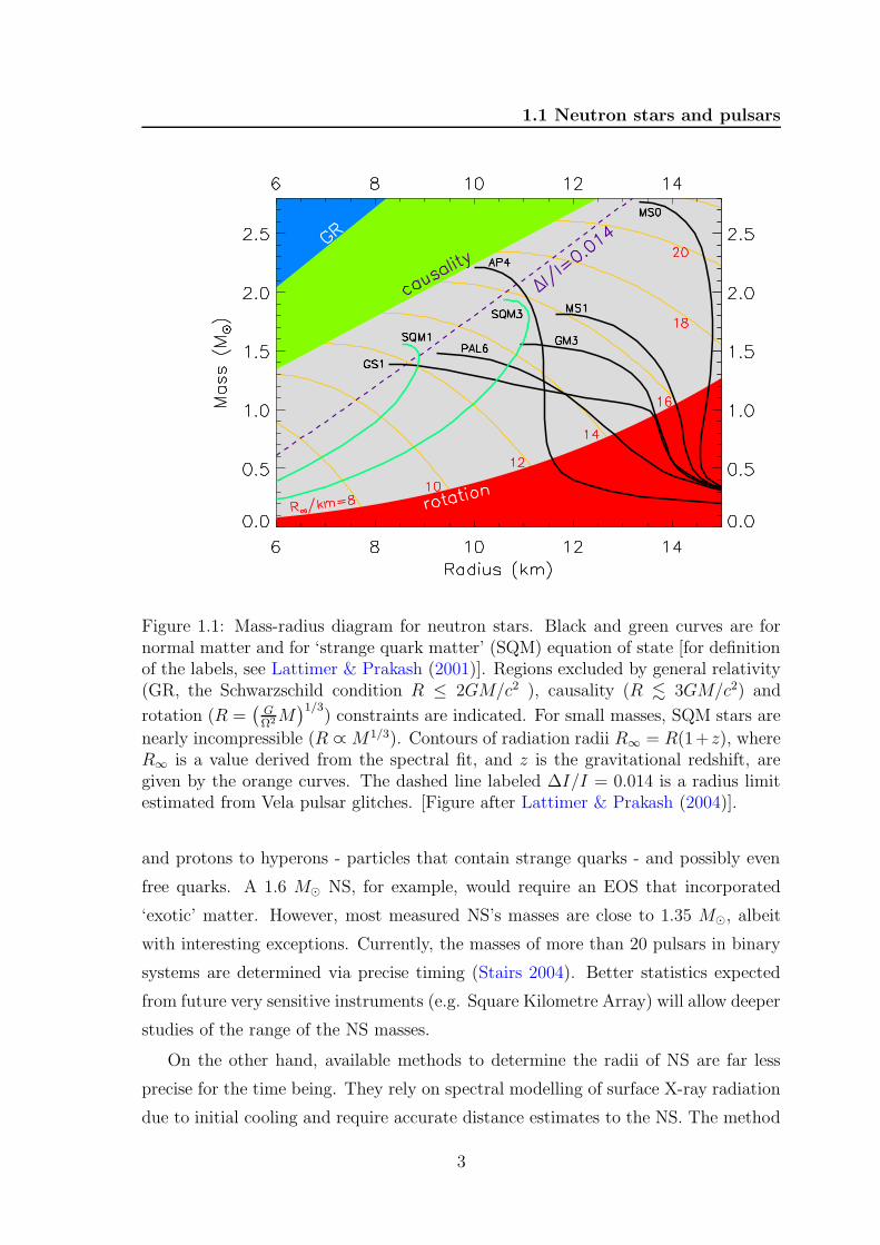
1.1 Neutron stars and pulsars
Figure 1.1: Mass-radius diagram for neutron stars. Black and green curves are fornormal matter and for ‘strange quark matter’ (SQM) equation of state [for definitionof the labels, see Lattimer & Prakash (2001)]. Regions excluded by general relativity(GR, the Schwarzschild condition R ≤ 2GM/c2 ), causality (R . 3GM/c2) and
rotation (R =(
GΩ2 M
)1/3) constraints are indicated. For small masses, SQM stars are
nearly incompressible (R ∝ M 1/3). Contours of radiation radii R∞ = R(1+z), whereR∞ is a value derived from the spectral fit, and z is the gravitational redshift, aregiven by the orange curves. The dashed line labeled ∆I/I = 0.014 is a radius limitestimated from Vela pulsar glitches. [Figure after Lattimer & Prakash (2004)].
and protons to hyperons - particles that contain strange quarks - and possibly even
free quarks. A 1.6 M NS, for example, would require an EOS that incorporated
‘exotic’ matter. However, most measured NS’s masses are close to 1.35 M, albeit
with interesting exceptions. Currently, the masses of more than 20 pulsars in binary
systems are determined via precise timing (Stairs 2004). Better statistics expected
from future very sensitive instruments (e.g. Square Kilometre Array) will allow deeper
studies of the range of the NS masses.
On the other hand, available methods to determine the radii of NS are far less
precise for the time being. They rely on spectral modelling of surface X-ray radiation
due to initial cooling and require accurate distance estimates to the NS. The method
3

1. INTRODUCTION
is biased by influence of strong gravity, as well as magnetised atmospheres of unknown
composition. Reliable measurements of NS radii are therefore, difficult to obtain and
to use them to constrain the models.
Milestones
Pulsar observations have given us by far the most accurate confirmation of general
relativity, and the first observations of the process of emission of gravitational waves,
as well as many other new astronomical data.
Pulsar research has been driven by numerous surveys with many different radio
telescopes over the years. These searches have discovered exciting new objects. At
the moment there are 1627 pulsars known. The most important discoveries of pulsar
radio astronomy are presented in Tab. 1.1.
Table 1.1: Milestones of pulsar radio astronomy (ordered chronologically)
Object DescriptionPSR B1919+21 Cambridge discovery of pulsars, Hewish et al. (1968)PSR B0531+21 Discovery of the Crab pulsar, Staelin & Reifenstein (1968)PSR B1913+16 The first binary pulsar; experimental demonstration of
the existence of gravitational waves, Hulse & Taylor (1974)PSR B1937+21 The first millisecond pulsar, ν = 642 Hz; for long time remains
the most rapidly spinning NS known, Backer et al. (1982)PSR B0540-69 The first extra-galactic pulsar, Seward et al. (1984)PSR B1821-24 The first pulsar in globular cluster, M21, Lyne et al. (1987)PSR B1257+12 The first pulsar planetary system; at the same time the first
extra-solar planetary system discovered,Wolszczan & Frail (1992)
PSR B1620-26 The first triple system: a pulsar, a white dwarf, anda Jupiter-mass planet, Backer et al. (1993),Thorsett et al. (1993)
PSR J0737-3039 The first ‘double pulsar’ system consisting of a 22.7 ms and2.77 s pulsars; gives even more stringent constrains ongravitational theories than PSR B1913+16Burgay et al. (2003), Lyne et al. (2004), Kramer et al. (2006)
PSR J1748-2446ad The fastest spinning pulsar, ν = 716 Hz, this pulsar locatedin Terzan 5 globular cluster beat the previous record of642 Hz from PSR B1937+21, Hessels et al. (2006)
4

1.1 Neutron stars and pulsars
Present surveys
Many of the discoveries in the past six years, including the discovery of the first
double pulsar J0737-3039 (see Tab. 1.1), were made using the 64-m Parkes telescope.
The Parkes multi-beam pulsar survey1 (PMBPS) is a sensitive survey of a strip along
the Galactic plane with |b| < 5 and l = 260 to l = 50. It uses the multi-beam
receiver system to collect data at 1.4 GHz from thirteen independent points in the
sky (Manchester et al. 2001). The 1.4 GHz operating frequency of the PMBPS is
particularly well suited for pulsar searches in the Galactic plane. Lower frequencies
suffer from deleterious effects of pulse broadening due to interstellar scattering and
dispersion, while pulsar flux densities typically are much reduced at higher frequen-
cies. Therefore, the strong inverse frequency dependence of scattering clearly favours
searches carried out at higher frequencies. More than one half of all known pulsars,
including the slowest radio pulsar (Young et al. 1999), have been discovered with this
system. Moreover, several pulsars with inferred magnetic field exceeding the critical
field of ∼ 4.3 × 10¹³ G were discovered. By this survey the large increase in the
number of nulling pulsars - where radio emission appears to abruptly ‘switch off’ for
many pulse period - is observed. The large number of radio pulsars discovered in this
survey resulted also in a number of candidate associations between young pulsars and
the unidentified EGRET sources. However, the EGRET sources have large positional
error, thus such associations naturally are uncertain. To confirm these matches we
need to wait for new γ-ray satellite missions like for example AGILE and GLAST
that will greatly reduce positional uncertainties.
On the other hand, the recently started Arecibo L-band Feed Array (ALFA) pul-
sar survey aims to find ∼ 1000 new pulsars (Cordes et al. 2006). The new survey is
enabled by several innovations. ALFA is a seven-beam feed and receiver system de-
signed for large-scale surveys in the 1.2–1.5 GHz band. The ALFA frontend is similar
to the 13-beam system used for the extremely prolific PMBPS and will complement it
in its sky coverage. Moreover, their initial and next-generation spectrometer systems
have much finer resolution in both time and frequency than the spectrometer used
with the PMBPS. This will allow to increase the detection volume of millisecond pul-
sars by an order of magnitude. Additionally, the sensitivity of the Arecibo telescope
allows for short pointings that simplify the detection of binary pulsars undergoing
strong acceleration. J. van Leeuwen et al. report already the results of their prelimi-
nary analysis: in the first months they have already discovered 21 new pulsars (van
1http://www.atnf.csiro.au/research/pulsar/pmsurv/
5

1. INTRODUCTION
Leeuwen et al. 2006).
Radio pulsars catalogues can be found in the archive maintained at the Parkes
Observatory operated by the Australia Telescope National Facility1 (ATNF) and at
the European Pulsar Network2 (EPN). Although, the EPN data base contains smaller
number of pulsars than the ATNF data base, it has a great advantage over the
Australian catalogue. It provides not only the basic pulsar parameters, but also pulsar
profiles at different frequencies, and in some cases the polarisation information, i.e.
intensity profiles for all Stokes parameters.
Current population studies of pulsars suggest that our Galaxy contains ∼ 105 −−106 active radio pulsars. Looking further ahead, the next-generation radio telescope
- the Square Kilometre Array3 (SKA) - is expected to detect essentially ∼ 20, 000 (for
some estimates even ∼ 30, 000 ) active radio pulsars. This telescope will have the
sensitivity of more than 100 times that of the Parks telescope and should be ready to
operate in 2015.
1.2 Observational characteristics of pulsars
Basic pulsar observables
Rotation-powered pulsars (RPPs) are generally referred to as ‘radio pulsars’, because
in the vast majority of cases, they are observed only just at radio wavelengths. Ro-
tational frequency ν (or corresponding period of rotation, P = 1/ν) is the basic
observational parameter of each pulsar. If possible its spin-down rate - first time
derivative of ν - is measured also. Additionally, for some pulsars the second fre-
quency derivative can be derived if only the regular, long term timing observations
are performed.
A neutron star spinning with angular velocity Ω = 2π/P , that decreases with time
at the rate of Ω = −2πP−2P < 0, loses its rotational energy Erot = 12IΩ2. Thus the
rate of the rotational kinetic energy loss is given by Erot = IΩΩ = −4π2IP /P 3 with
the assumption that stellar moment of inertia I = kMNSR2NS is constant, i.e. does
not change with time. Coefficient k amounts to 0.4 for a sphere of uniform density
distribution. For a NS, the exact value of k depends on the density profile, hence, on
the equation of state. For most practical calculations I ' 1045 g cm2 is derived from
the canonical NS parameters, MNS = 1.4 M, RNS = 10 km and k = 0.4.
1http://www.atnf.csiro.au/research/pulsar/psrcat/2http://www.mpifr-bonn.mpg.de/div/pulsar/data/3http://www.skatelescope.org/
6

1.2 Observational characteristics of pulsars
The so called spin-down luminosity Lsd is directly related to the rotational kinetic
energy loss rate by
Lsd = |Erot| ' 3.95 × 1031I45P−15P−3 erg s−1 (1.1)
where P is in seconds, P−15 ≡ P /10−15 and I45 ≡ I/1045 g cm2. One way of estimating
pulsar magnetic field is to equate the rotational energy loss rate (Eq. 1.1) with that
from a classical magnetic dipole radiation of a rotating magnetic dipole (Eq. 1.2).
This estimate was first given by Ostriker and Gunn (Ostriker & Gunn 1969). The
dipole (which represents the star) with its magnetic moment set by BsR3NS, rotating
in vacuum will lose energy at the rate
Lmagn =2
3c3B2
s sin2 αR6NSΩ4, (1.2)
where α is an inclination angle between the dipole magnetic axis and the spin axis,
and Bs is the strength of the magnetic field at the equator of the neutron star.
Consequently, the inferred surface dipolar magnetic field Bs for an orthogonal rotator
case, i.e. α = 90, is
Bs ' 1012
√
PP−15 G (1.3)
for I45 = 1 and RNS = 10 km. Another model for estimating the pulsar magnetic
field, where the dipolar radiation is replaced with a magnetospheric wind of particles,
leads to a similar result, but it is independent of the inclination angle α.
Those two simple models give a differential equation for period P :
P = KP−1, (1.4)
where Bs is now hidden in the parameter K.
This is a special case within the more general model for magnetic braking, which
reads
P = KP 2−n. (1.5)
The parameter n is the braking index that reflects the true spin-down behaviour and
K is usually assumed to be constant. For the simple model discussed above n = 3.
In terms of ν the equation 1.5 corresponds to
ν = −Kνn. (1.6)
The braking index can be determined, if in addition to ν, the second derivative of the
spin frequency ν can be obtained from radio timing observations. By differentiating
7

1. INTRODUCTION
Eq. 1.6 and eliminating constant K, the braking index is related with the pulsar
rotational parameters via
n =νν
ν2. (1.7)
Usually, the observed ν is contaminated by timing noise, therefore to get reliable value
a long observational time span is needed. Thus, only for a few pulsars a determination
of n has been possible. The values range from n = 1.4 to n = 2.9 (e.g. Kaspi & Helfand
2002).
By integrating Eq. 1.5 with the assumption of a constant K and n 6= 1 we obtain
the age of the pulsar
T =P
(n − 1)P
[
1 −(
P0
P
)n−1]
. (1.8)
However, the spin period at birth P0 is unknown. Assuming that the initial period
is negligibly short (P0 P ) and taking the braking index n = 3 the above equation
leads to the so-called characteristic age
τc 'P
2P' 15.8
P
P−15
Myr, (1.9)
also known as the spin-down age. This quantity does not necessarily provide a reliable
age estimate. For the Crab pulsar τc ' 1240 yr, which is comparable to the age of
about 950 years known from the Chinese observation of the supernova explosion.
However, for some other objects larger discrepancies are known.
The pulsar magnetosphere is bounded by the ‘light cylinder’ of radius
RLC =cP
2π' 4.77 × 10⁴P km, (1.10)
which is the distance from the spin axis at which the co-rotational speed equals the
speed of light and it sets a natural limit on the size of the neutron star magnetosphere.
The magnetic field strength at the light cylinder is given by
BLC = Bs
(
ΩRNS
c
)3
≡ Bs
(
2πRNS
cP
)3
' 9.2P−5/2P−15 G. (1.11)
All field lines which cross the light cylinder are then considered as open lines, and
their footpoints on the stellar surface define two polar caps of radius
RPC =
√
2πR3NS
cP≡ RNS
√
RNS
RLC' 150P−1/2 m. (1.12)
8

1.2 Observational characteristics of pulsars
The P–P diagram
The observed pulsar spin period P as well as the corresponding rate of spin-down P
can be obtained with very high accuracy through regular radio timing measurements.
These values give us insights into the pulsar spin evolution. The best way to present
it is to use the ‘P–P diagram’ shown in Fig. 1.2. Two main groups of pulsars are
clearly visible. The most numerous group is the group of ∼ 1500 ‘normal pulsars’
(P ∼ 0.5 s and P ∼ 10−15 s s−1) out of 16271 already known. Within this class of
pulsars we can distinguish three subclasses. RPPs are called either young, or middle-
age, or old if their spin-down age (Eq. 1.9) is of order a few times 103−104, 105−106,
and ≥ 106 years, respectively. Their inferred magnetic fields (Eq. 1.3) span the range
from ∼ 1011 G to ∼ 1013 G. The second group, occupying the lower left part of the
diagram, contains a hundred of ‘millisecond pulsars’ (P ∼ 5 ms and P ∼ 10−20 s s−1).
Their inferred magnetic fields span the range from ∼ 108 G to ∼ 1010 G. In addition to
rotational characteristics, a very important difference between normal and millisecond
pulsars (MSPs) is binarity of most of the MSPs. The orbiting companions are either
white dwarfs, main sequence stars or other NSs (i.e. double neutron stars binaries -
DNS). Evolutionary, it is possible that some binaries include a black-hole companion.
However, this kind of systems still remains the Holy Grail in pulsar astronomy.
The range of spin-down luminosity values Lsd covered by known pulsars is impres-
sively wide. The largest value, Lsd ' 4 × 1038 erg s−1, is reached by the Crab pulsar
and PSR J0537-6910. The minimal value, Lsd ' 4 × 1028 erg s−1, is ten orders of
magnitude smaller and it is reached by the slowest radio pulsar detected so far (PSR
J2144-3933, P ∼ 8.5 s, Young et al. (1999)).
The DNS group, placed on the P − P diagram between normal and MSPs, is
a rather small group (eight members), but certainly not negligible. On the P − P
diagram the DNS pulsars are located near the line of a constant magnetic field of
1010 G. An excellent example of DNS is the original binary pulsar B1913+16 (Tab. 1.1)
in which the orbital period is observed to decrease at the rate predicted by general
relativity due to emission of gravitational waves (Taylor & Weisberg 1989). So far
only in one system, PSR J0737-3039, two pulsars (named A and B) are observed.
This system turned out to be the best testbed for the theory of General Relativity.
In particular, the Shapiro delay measured for this system remains in agreement with
the delay predicted by GR with an uncertainty of ∼ 0.05% (Kramer et al. 2006).
1According to The Australia Telescope National Facility Pulsar Catalogue,http://www.atnf.csiro.au/research/pulsar/psrcat/, Manchester et al. (2005).
9

1. INTRODUCTION
Figure 1.2: The P − P diagram showing the current sample of radio pulsars. Binarypulsars are marked as an open circle. Pulsars associated with supernova remnant aremarked with stars. For soft gamma repeaters (SGRs) and anomalous X-ray pulsars(AXPs) open triangles are used, whereas ‘radio-quite’ pulsars are highlighted withfilled triangles. Lines of constant magnetic field Bs (Eq. 1.3) and characteristic age τc
(Eq. 1.9) are indicated. Regions indicated with grey are areas where radio pulsars arenot predicted to exist by theoretical models. The ‘spin-up’ line denotes the terminalperiod for objects moving to the left in the diagram due to accretion and become‘recycled’ millisecond pulsars once it ceases. The ‘graveyard’ marks the region whereradio pulsars emit less radiation or turn off entirely. [Courtesy M. Kramer].
10

1.2 Observational characteristics of pulsars
Moreover, observations of relativistic effects in binary pulsars like J0737-3039 allow
precise determination of their masses.
Pulsars are ‘born’ with very short rotation periods P0, of the order of 1 to 10 mil-
liseconds, and large slow down rates P0 of the order of ∼ 10−9 s s−1 to ∼ 10−12 s s−1.
Then, they slow down along the lines of constant magnetic field values (Eq. 1.3).
Their magnetic fields may decay on time scales longer than 1 Myr. When they cross
the pulsar ‘death line’, the conditions for the pair creation are not fulfilled any more,
therefore no radio emission is produced and the pulsars become invisible. The lower
right region on the P − P diagram defined by the ‘death line’ is commonly called a
‘graveyard’. In the standard picture all pulsars start as normal pulsars. Millisecond
pulsars are also called ‘recycled pulsars’ due to their evolutionary path. It is be-
lieved that future MSPs enter the ‘graveyard’ as members of binary systems. As the
companion evolves, mass and angular momentum are transfered from the companion
to the pulsar, spinning it up. Once ‘spun-up’, the pulsar is ‘recycled’ as a millisec-
ond pulsar. This model predicts that all millisecond pulsars are members of binary
systems.
Additionally, in the upper right part of the diagram a group extraordinary of ob-
jects is located: the Soft Gamma Repeaters (SGRs) and Anomalous X-ray Pulsars
(AXPs). SGRs emit bright, repeating flashes of low-energy (soft) gamma rays. The
physical nature of these stars was a mystery for many years. Late in 1992, it was
proposed that SGRs are magnetically-powered neutron stars, or magnetars. Sub-
sequent observational studies support this hypothesis. AXPs are also magnetars –
young, isolated, highly magnetised neutron stars. These energetic X-ray pulsars are
characterised by slow rotation periods of ∼ 5 − 12 s and large magnetic fields of
∼ 1013 − 1015 G, some have also been found to emit SGR-like bursts. Very likely,
SGRs and AXPs are essentially connected to each other. Their behaviour is now best
described by the magnetar model, in which the decay of an ultra-strong magnetic
field (B & 1014 G) powers the high-luminosity bursts and also a substantial fraction
of their X-ray emission. For the recent review about these sources see Woods &
Thompson (2004).
There are also pulsars, for which the pulsations have been detected at high energies
but not at radio frequencies. In most cases such pulsation are seen in the X-ray regime.
This may be due to a misaligned radio beam or due to very low radio luminosity.
Pulsars characterise by this behaviour are called ‘radio quiet’ pulsars. A prototype
of this group is a well known Geminga pulsar.
11

1. INTRODUCTION
1.3 Distribution of pulsars in the Galaxy
Most of known pulsars are Galactic, residing in or near the disc of the Galaxy. Some of
them (millisecond pulsars) are located in globular clusters. Twenty pulsars have been
found to date in the Magellanic Clouds (Manchester et al. 2006). No pulsars have been
detected in other galaxies. The reason is a limited sensitivity of radio telescopes in
confrontation with pulsars as actually very weak radio sources. Moreover, propagation
effects make the task of finding pulsed emission from distant sources more difficult.
For these reasons we observe only a tiny fraction of a much larger pulsar population.
The observed pulsar sample is biased towards the brighter and nearby objects that are
easiest to detect. The extent to which the sample is incomplete is well demonstrated
by the projection of all pulsars known to date onto the Galactic plane in Fig. 1.3 left
panel. The gathering of pulsars around the Sun clearly differs from the distribution
of other stellar populations that show a radial distribution about the Galactic centre.
Their cumulative number distribution as a function of distance from the Galactic
centre is shown in Fig. 1.3, middle panel, solid red line. This may be compared with
the simulated distribution of pulsars with no selection effects (Fig. 1.3, middle panel,
dotted black line). A strong deficit in the observed number distribution becomes
visible beyond a few kpc. Very sensitive SKA pulsar survey will allow to discover
∼ 20, 000 pulsars including ∼ 1, 000 millisecond pulsars (Fig. 1.3, right panel). The
SKA will provide a complete sampling of pulsars in both the Galaxy and in Galactic
globular clusters. Information collected by the SKA will provide a detailed map
of electron density and magnetic fields in the Galaxy, the dynamics of the pulsar
systems, and their evolutionary history. A huge sample of detected pulsars will allow
statistical studies of pulsars.
1.4 Pulsars across the electromagnetic spectrum
Pulsars are known emitters across the whole electromagnetic spectrum. They are ob-
served not only in the radio band, but also in optical, X-rays and γ-rays. In contrast
to more than 1600 pulsars already detected in radio, we know just six optical pulsars,
around eighty X-ray pulsars, and seven (high-confidence) gamma-ray pulsars. The
pulsars seen in optical are: Crab, Vela, Geminga, PSR B0540-69, PSR B0656+14
and PSR B1929+10 (e.g. Mignani et al. 2004; Shearer & Golden 2002). The first
four objects show clear pulsed emission. PSR B0656+14 and PSR B1929+10 are less
12

1.4 Pulsars across the electromagnetic spectrum
−15 −10 −5 0 5 10 15X (kpc)
−15
−10
−5
0
5
10
15
Y (
kpc)
Figure 1.3: Left : The current sample of all known radio pulsars projected onto theGalactic plane. The Galactic centre is at (0, 0) and the Sun is at (0, 8.5) kpc.Middle: Cumulative number of pulsars as a function of projected distance from theSun. The solid red line shows the observed sample while the dotted black line showsa model population free from selection effects. [Reproduced from Lorimer (2005)].Right : Simulated pulsar population projected onto Galactic plane. The ∼ 20, 000pulsars estimated to be discovered by SKA survey are shown together with the spiralarms structures. Coordinates are the same as on the left panel. [Credit Cordes et al.(2004)].
clear cases in terms of pulsed versus unpulsed character of their emission. In partic-
ular, PSR B1929+10 proper motion yielded the confirmation of its optical counter-
part (Mignani et al. 2002), but only a marginal detection of optical pulsations exists
(Mignani, private communication). The brightest pulsed source is the Crab pulsar. It
is strong enough to allow extensive studies of its single pulses. Moreover, it is the only
pulsar for which phase-resolved polarisation characteristics could have been obtained
(Jones et al. (1981), Smith et al. (1988), and very recent results by A. S lowikowska,
see Chap. 3).
In the past decade we observed the growing number of RPPs detected in X-rays.
It is mostly due to recent observations performed by sensitive instruments on board
the XMM-Newton and Chandra satellites (∼ 80 pulsars). ROSAT and ASCA yielded
‘only’ 33 detections, including 7 X-ray pulsars that were already known from earlier
missions - the Einstein X-Ray Observatory and EXOSAT. X-ray observations of pul-
sars offer more direct insight into the magnetospheric plasma densities and processes
in comparison to not fully understood coherent radio emission. However, in many
pulsars the observed X-ray emission is a mixture of thermal and non-thermal emis-
sion that can not always be discriminated by the available data. Thermal emission
may originate from the stellar surface as a consequence of stellar interior cooling.
Additionally, it may be caused by heated polar caps due to backflowing particles.
13

1. INTRODUCTION
In the latter case X-ray flux modulation are expected due to rotation. In any case,
the thermal emission from pulsars is expected to deviate from a simple blackbody
radiation; significant modifications are due to presence of a magnetised atmosphere
on the NS surface. In contrast to thermal X-rays, non-thermal X-ray emission, as
well as gamma-ray emission, is exclusively a direct consequence of magnetospheric ac-
tivity of the pulsar. For different models different regions in pulsars magnetospheres
are considered as a particle accelerators. Particles are accelerated to ultrarealtivistic
energies, and in turn they induce electromagnetic cascades with curvature radiation,
synchrotron radiation, and radiation due to inverse Compton scattering. The non-
thermal emission spreads then from optical, through X-rays, to γ-rays frequencies.
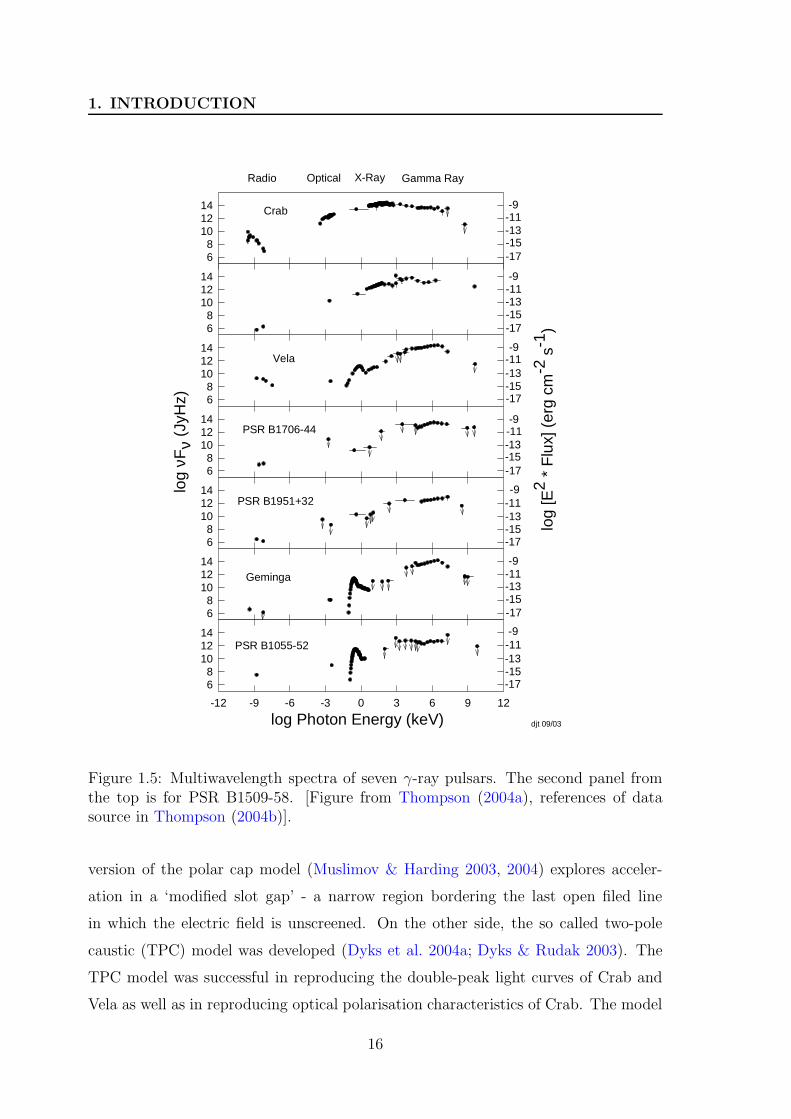
For seven pulsars - Crab, B1509-58, Vela, B1706-44, B1951+32, Geminga and B1055-
52 - strongly pulsed gamma-ray emission was detected (e.g. Kanbach 2002). Their
light curves and phase-averaged spectral energy distributions from radio to gamma-
rays are presented in Figs. 1.4 and 1.5, respectively. Important features of these light
curves are: (a) for each pulsar the pulse shape changes with energy, sometimes very
dramatically; (b) not all seven objects are seen at hard γ-ray energies - the case of
PSR B1509-58, (c) three pulsars (Crab, Vela and Geminga) show a common feature
above 100 MeV: a double peak structure.
The energy spectra in Fig. 1.5 show the distinction between the radio emission
(that originate from a coherent emission) and the high-energy emission (originating
in incoherent processes). It is particularly visible for the Crab and Vela pulsar.
These spectra clearly emphasise that the emission in X-rays and γ-rays dominates
the radiation budget of these pulsars. The spectra of the pulsed emission are generally
harder than a power law spectrum with a photon index of −2 (which would give a
horizontal line in the spectral plot). The spectra have a cut-off or a turnover at a few
GeV (with the exception of PSR B1509-58 mentioned before). Their interpretation
is model dependent.
The emission processes in the magnetospheres of RPP have been studied in great
details from many years. Yet, they are still not well understood. The radio emis-
sion must be a coherent process requiring significant particle densities and probably
electron-positron pairs, and the emission at higher energies requires acceleration of
particles to energies of at least ∼ 10 TeV.
Several mechanisms of the radio emission have been proposed. These are: maser
curvature emission, linear acceleration emission, anomalous Doppler instability, cur-
vature-drift instability and relativistic plasma emission (review Melrose 2004).
14

1.4 Pulsars across the electromagnetic spectrum
Crab B1509-58 Vela B1706-44
X-ray/Gamma Ray
HardGamma Ray
B1951+32 Geminga B1055-52
Radio
Optical
SoftX-Ray
?
djt 9/03P ~ 33 ms P ~ 89 ms P ~ 102 ms P ~ 39 ms P ~ 237 ms P ~ 197 msP ~ 150 ms
Inte
nsity
var
iatio
n du
ring
one
rota
tion
of th
e ne
utro
n st
ar
Figure 1.4: Light curves of seven γ-ray pulsars in five energy bands (given on the rightside of the plot), from left to right in order of characteristic age τc (Eq. 1.9). Eachpanel show one full rotation of the neutron stars. [Figure from Thompson (2004a),references of data source in Thompson (2004b)].
The models of pulsed high-energy emission are based on physics of particle ac-
celeration, which results from the strong electric fields that are induced along open
magnetic field lines. Two accelerator sites have been studied in details and two main
types of models have been developed: polar cap models and outer gap models. Polar
cap models are based on particle acceleration near the magnetic poles (Ruderman &
Sutherland 1975) and outer gap models are based on acceleration in vacuum gaps
in the outer magnetosphere (Cheng et al. 1986; Romani 1996). Additionally, pulsed
emission from the wind zone, the striped wind model, has also been proposed (Petri
& Kirk 2005). Both types of models significantly evolved in recent years. More recent
15
1. INTRODUCTION
68
101214
68
101214
68
101214
Radio Optical X-Ray Gamma Ray
68
101214
log
νFν
(JyH
z)
68
101214
log Photon Energy (keV)-12 -9 -6 -3 0 3 6 9 12
68
101214
Crab
PSR B1509-58
PSR B1951+32
Vela
PSR B1706-44
Geminga
PSR B1055-52
djt 09/03
-9-11-13-15-17
-9
-9
-9
-9
-9
-9-11
-11
-11
-11
-11
-11
-13
-13
-13
-13
-13
-13
-15
-15
-15
-15
-15
-15
-17
-17
-17
-17
-17
-17
log
[E2 *
Flu
x] (
erg
cm-2
s-1
)68
101214
Figure 1.5: Multiwavelength spectra of seven γ-ray pulsars. The second panel fromthe top is for PSR B1509-58. [Figure from Thompson (2004a), references of datasource in Thompson (2004b)].
version of the polar cap model (Muslimov & Harding 2003, 2004) explores acceler-
ation in a ‘modified slot gap’ - a narrow region bordering the last open filed line
in which the electric field is unscreened. On the other side, the so called two-pole
caustic (TPC) model was developed (Dyks et al. 2004a; Dyks & Rudak 2003). The
TPC model was successful in reproducing the double-peak light curves of Crab and
Vela as well as in reproducing optical polarisation characteristics of Crab. The model
16
1.5 The Crab pulsar and its nebula
stimulated a significant revision of outer gap models very recently.
So far none of the proposed models is able to reproduce all observational pul-
sar features, i.e. their light curves, spectra (also phase resolved) and polarisation
properties.
1.5 The Crab pulsar and its nebula
The Crab pulsar is surrounded by bright diffuse nebula, that is about six light years
across, and expands outward at 4.8 million km per hour. The filamentary system
visible in optical is near the outer boundary of this expansion. Both, the Crab Nebula
and the pulsar are bright sources of non-thermal radiation extending from radio to
gamma-rays (the nebula was the first TeV source detected in the sky).
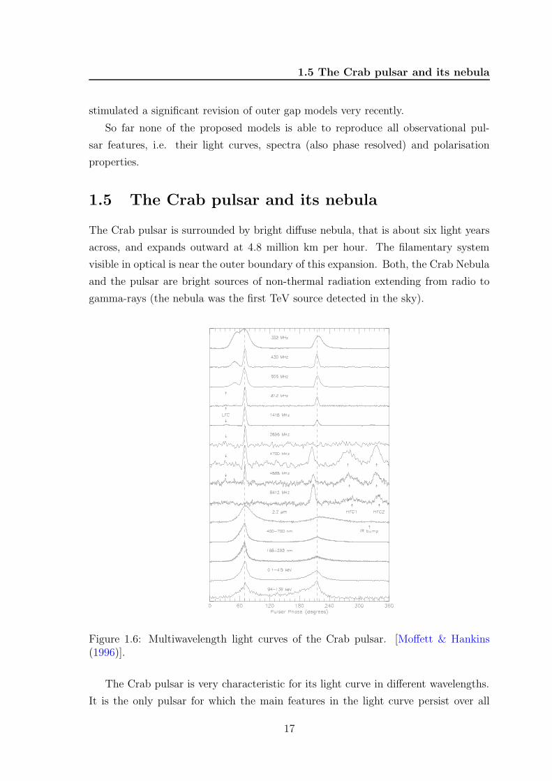
Figure 1.6: Multiwavelength light curves of the Crab pulsar. [Moffett & Hankins(1996)].
The Crab pulsar is very characteristic for its light curve in different wavelengths.
It is the only pulsar for which the main features in the light curve persist over all
17

1. INTRODUCTION
wavelengths, from radio to gamma-rays. The light curve shows two basic components
- the main pulse (MP) and the inter pulse (IP). This double-peak structure remains
phase-aligned over all available wavelengths (Figs. 1.4 and 1.6). However, there are
some extra features present: at low radio frequencies a precursor to the first peak is
visible. Moreover, an additional low frequency component (LFC) is present between
1 and 5 GHz. Above 4.7 GHz two additional components trailing the IP show up.
They are known as high frequency components: HFC1 and HFC2. In the optical
domain the light curve is much less structured than in radio. Both, the MP and the
IP are slightly asymmetrical: in the MP the signal falls off more sharply that it rises,
whereas the opposite situation prevails for the IP. The peak of the MP is surprisingly
sharp, and it plummets down in only 40 µs. The X-ray shape is interesting because
both the MP and the IP are of about the same intensity. There is a ‘bridge’ component
between the MP and the IP at high energies. At optical and X-rays the flux level
before the MP never reaches the zero level (Golden et al. 2000a; Tennant et al. 2001).
Presently there is no theoretical concept that would explain all these extra features
in the Crab light curve.
The Crab pulsar emits maximum power at about 100 keV (Fig. 1.5). Its spectrum
can be well described by a broken power law extending from the optical (∼ 1 eV)
to about 10 GeV. In addition to the pulsed emission the Crab pulsar shows a strong
unpulsed component at high energies. This component has been interpreted as coming
from the inner part of the Crab Nebula: as synchrotron radiation below a few GeV and
as inverse Compton radiation, upscattered from optical photons, up to TeV energies.
Comparison of the X-ray, optical, infrared, and radio images of the Crab Nebula
shows that it is most compact in X-rays and largest in the radio (Fig. 1.7). The X-ray
nebula shown in the Chandra image is about 40% as large as the optical nebula, which
is in turn about 80% as large as the radio image. Chandra’s X-ray image of the Crab
Nebula directly traces the most energetic particles being produced by the pulsar.
This image reveals an unprecedented level of details about how the energetic wind of
particles (mostly electrons) interacts with the nebular matter and its magnetic field.
While the electrons move outward, they lose energy to radiation. The diffuse optical
light comes from intermediate energy particles produced by the pulsar. The optical
filaments are identified as expanding gases, consisted of the matter that was once
ejected by the supernova explosion. The gas temperature is of the order of tens of
thousand degrees Kelvin. The infrared radiation comes from dust grains mixed in
with the hot gas in the filaments. Radio waves can travel the largest distance and
define the full extent of the nebula.
18
1.6 An outline of the thesis and statement of originality
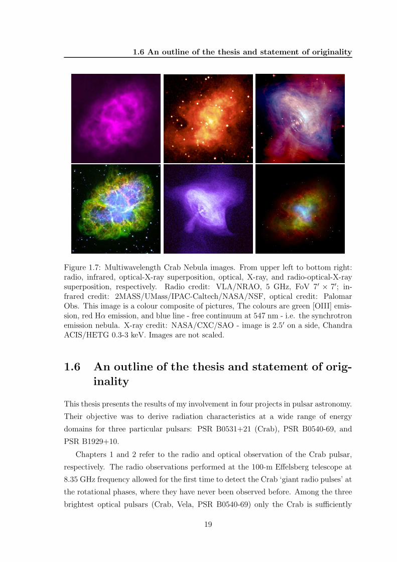
Figure 1.7: Multiwavelength Crab Nebula images. From upper left to bottom right:radio, infrared, optical-X-ray superposition, optical, X-ray, and radio-optical-X-raysuperposition, respectively. Radio credit: VLA/NRAO, 5 GHz, FoV 7′ × 7′; in-frared credit: 2MASS/UMass/IPAC-Caltech/NASA/NSF, optical credit: PalomarObs. This image is a colour composite of pictures, The colours are green [OIII] emis-sion, red Hα emission, and blue line - free continuum at 547 nm - i.e. the synchrotronemission nebula. X-ray credit: NASA/CXC/SAO - image is 2.5′ on a side, ChandraACIS/HETG 0.3-3 keV. Images are not scaled.
1.6 An outline of the thesis and statement of orig-
inality
This thesis presents the results of my involvement in four projects in pulsar astronomy.
Their objective was to derive radiation characteristics at a wide range of energy
domains for three particular pulsars: PSR B0531+21 (Crab), PSR B0540-69, and
PSR B1929+10.
Chapters 1 and 2 refer to the radio and optical observation of the Crab pulsar,
respectively. The radio observations performed at the 100-m Effelsberg telescope at
8.35 GHz frequency allowed for the first time to detect the Crab ‘giant radio pulses’ at
the rotational phases, where they have never been observed before. Among the three
brightest optical pulsars (Crab, Vela, PSR B0540-69) only the Crab is sufficiently
19

1. INTRODUCTION
bright for individual pulse work to be performed. Furthermore, it is the only pulsar
for which the Stokes parameters can be accurately measured throughout the pulsar’s
rotation period. Optical polarisation of the Crab pulsar, obtained with 30 µs time
resolution is presented and discussed in Chapter 2. The next two chapters refer to the
X-ray observations. Chapter 3 is dedicated to the PSR B0540-69 results obtained from
the INTEGRAL satellite, whereas Chapter 4 presents the results of the reanalysis of
the available X-ray archive data of PSR B1929+10.
Three projects (Chapters 1 to 3) started with observational campaigns and were
followed by data reduction and data analysis. In all these cases I have been assisted
by other members of observational proposals submitted in order to obtain telescope
time. The remaining project (Chapter 4) consisted of data reduction and analysis.
My analysis was carried out mostly at the Department of Astrophysics, Nicolaus
Copernicus Astronomical Center Torun, and at MPE-MPG Garching between 2001
and 2006.
Except where otherwise acknowledged, the work presented in this thesis is my
own. Significant contributions from other people are as follows:
Chapter 1: Effelsberg proposal to detect giant radio pulses from the Crab pulsar;
PI of the proposal: A. S lowikowska. Other members of the team: Dr. Axel
Jessner (MPIfR) performed the observations; together with Dr. Bernd Klein
(MPIfR) he installed and run, for the first time, the Le Croy oscilloscope at
the 100-m Effelsberg radio telescope; during the data analysis I have used some
scripts written by Axel Jessner.
Chapter 2: Optical polarimetric observations with Nordic Optical Telescope;
PI of the proposal: Dr. G. Kanbach (MPE). The observations were performed
jointly by all members of the team: G. Kanbach, A. S lowikowska, A. Stefanescu
(MPE) and Fritch Schrey (MPE).
Chapter 3: INTEGRAL observations of PSR B0540-69; PI of the proposal: Dr.
G. Kanbach. The RXTE ephemeris of PSR B0540-69 used in my analysis were
derived by Dr. Lucien Kuiper (SRON).
Chapter 4: Lucien Kupier performed the analysis described in the Appendix B.
For some parts of data analysis I used his scripts.
20

Chapter 2
Enhanced radio emission from theCrab pulsar
2.1 Introduction
The occurrence of sporadic radio emission of very strong pulses by NP 0532, the
very first name of the Crab pulsar, has been known since its discovery by Staelin
and Reifenstein (Staelin & Reifenstein 1968). They discovered the dispersed pulse
signals from the Crab Nebula. These strong pulses were not periodic (see Fig. 2.1),
therefore the rotational period of the Crab was not established. However, considering
the source as a periodic one, Staelin and Reifenstein were able to give the upper limit
of 0.13 s for its period. Noteworthy is that the pulsar would not have been discovered
if it had not shown the strong radio pulses, that were later called the giant radio
pulses (GRPs). A single pulse of average flux density can not be detected because of
the high radio emission from the plerionic nebula. The strongest pulses exceed the
total radio emission from the nebula itself by an order of magnitude. For a long time
it was the only known pulsar showing the GRP phenomenon. The rotational period
of the pulsar was measured by Comella, who used the 305 m reflector at the Arecibo
Observatory (Comella et al. 1969), whereas its slowdown rate was given by Richards
and Comella a few months later (Richards & Comella 1969). The optical emission
was for the first time reported by Cocke, Disney and Taylor (Cocke et al. 1969), and
later confirmed by other groups (e.g. Nather et al. 1969). Fishman, Harnden and
Haymes reported the detection of the pulsar at hard X-rays (Fishman et al. 1969),
Bold, Desai and Holt, as well as Fritz et al. in soft X-rays (Boldt et al. 1969; Fritz
et al. 1969), and Neugebauer et al. in the infrared wavelengths (Neugebauer et al.
1969).
21

2. ENHANCED RADIO EMISSION FROM THE CRAB PULSAR
Figure 2.1: Time-frequency diagram of radio pulses observed with circular polarisa-tion. Left: One strong and three week pulses (marked with arrows) received fromPSR B0531+21 on 21 October 1968. Right: One typical pulse received from PSRB0531+21 on 19 October 1968. Open squares and closed circles represent deviationsfrom the mean of 4.2 and 8.3 σ, respectively. Horizontal axis is a time scale in seconds.Within one second the Crab pulsar rotates around 30 times. [Staelin & Reifenstein(1968)].
Following studies of its pulse shape as a function of radio frequency have shown
that Crab is very unique (Figs. 2.2, 2.3). The average pulse profile is determined
by averaging the data from thousands of sequentially recorded single pulses. The
results show that the averaged radio pulse profile consists of two main components:
an intense but narrow ‘main pulse’ (MP), lasting about 250 µs with respect to the
33 ms pulsar period, and a broader and weaker ‘inter pulse’ (IP) following the MP
by 13.37 milliseconds. IP does not occur exactly between successive main pulses;
the phase separation between the MP and the IP is ∼ 0.4. At lower frequencies
∼ 300 − 600 MHz another broad and weak component is visible. It precedes the MP
by 1.6 milliseconds. It is called ‘precursor’ (P). New and unseen before 1996 profile
components were discovered by Moffett and Hankins, Fig. 2.3 (Moffett & Hankins
1996). In the average pulse shape at 1.4 GHz the precursor vanishes, due to its
steep spectral index, leaving only the MP, IP, and a weak but distinct low frequency
component (LFC). It is ∼ 36 ahead of the MP, therefore it is not coincident with
the position of the precursor apparent at lower frequency (Fig. 2.3, second panel from
the top). Two additional components appear in the profiles obtained for frequencies
between 5 and 8 GHz. These two broad components with nearly flat spectrum are
referred to as high frequency component 1 and 2, i.e. HFC1 and HFC2, respectively.
The existence of the extra components at high frequency and their strange, frequency-
dependent behaviour is unlike anything seen in other pulsars. It can not easily be
22

2.1 Introduction
Figure 2.2: Average Crab pulsar pulse shape at 73.8, 111.5, 196.5, 318, and 430 MHz,respectively from the top to the bottom. Phases of pulses are arbitrary. [Rankin et al.(1970)].
explained by emission from a simple dipole field geometry. Two main components,
i.e. the MP and the IP, have counterpart non-thermal emission from the infrared to
the gamma-ray energies (Fig. 1.6).
The pulse shape changes markedly across all radio frequencies (Fig. 2.3). The
changes are caused by intrinsic as well as propagation effects. At lower frequen-
cies the pulse shape becomes more washed out as the well-defined features seen at
430 MHz broaden (Fig. 2.4). These changes are due to the effects of radio wave prop-
agation in the interstellar medium between the Earth and the pulsar (e.g. Lorimer
& Kramer 2005). Individual waves from the pulsar get scattered by the electrons in
the interstellar medium, and thus the signal that actually reaches the radio telescope
is the superposition of signals from very many slightly different paths through the
medium. At a sufficiently low frequency the waveform will be smeared out so much
as to be indistinguishable from continuous steady emission. This effect is illustrated
in Fig. 2.4. The strong inverse frequency dependence of scattering clearly favours
pulsar searches carried out at high frequencies. Besides scattering, two other dis-
tinct propagation effects occur: dispersion and scintillation. The dispersion effect is
a frequency dependence of the radio waves group velocity as they propagate through
23

2. ENHANCED RADIO EMISSION FROM THE CRAB PULSAR
Figure 2.3: The aligned, average radio intensity profiles of the Crab pulsar obtained at0.33, 1.4, 4.9 and 8.4 GHz with Very Large Array (VLA) showing several components:the main pulse (MP), interpulse (IP), precursor (visible at 330 MHz, just before MP),low frequency component (LFC), and two broad high frequency components (HFC1,HFC2), waxing and waning with radio frequency.[Moffett & Hankins (1996)].
the ionised component of the interstellar medium (ISM). The delay in pulse arrival
time is inversely proportional to observing frequency, thus pulses observed at higher
frequencies arrive earlier at the telescope than their lower frequency counterparts.
During the observations the de-dispersion procedure is used to correct for this effect.
Because the ISM is highly turbulent and inhomogeneous, its irregularities produce
phase modulation on the propagating pulsar signal. This scintillation effect causes
the observed intensity to fluctuate on a variety of timescales and bandwidths.
(Comment: Figs. 2.1, 2.2, 2.4 and 2.5 are reproduced from papers published in
late 60’s and early 70’s. Because the only available source of these figures are scanned
images, therefore they are of poor quality.)
24

2.1 Introduction
Figure 2.4: (a) Intrinsic pulse shape assumed in the broadening model. In (b) and(c) the intrinsic pulse is convolved with an exponential and an xe−x probability-density function, respectively, representing multi-path propagation effects in the in-terstellar medium. (b) and (c) are also convolved with functions representing thepulse-broadening effects of the radiometer, and are thus directly comparable with theobserved pulses in Fig. 2.2. [Rankin et al. (1970)].
25

2. ENHANCED RADIO EMISSION FROM THE CRAB PULSAR
2.2 Giant radio pulses
For over 25 years, only the Crab pulsar was known to emit GRPs. Actually, it
was discovered because of its giant radio pulses at the phases of MP. Its individual
GRPs might last just a few microseconds (Hankins et al. 2003). However, they rank
among the brightest flashes in the radio sky reaching peak flux densities of up to
1500 Jy even at high radio frequencies. Already four years after its discovery it
has been reported that GRPs occur not only at the MP, but also at the IP phases
(Gower & Argyle 1972). This discovery is illustrated in Fig. 2.5. Until 2005 the GRP
phenomenon in the Crab pulsar had been known to occur exclusively at the phases
of the MP and the IP (Cordes et al. 2004; Lundgren et al. 1995; Sallmen et al. 1999).
In particular, no GRPs had been detected either in the LFC or at the phases of the
high radio frequency components: HFC1 and HFC2. This situation has changed due
to the results published by Jessner, S lowikowska et al. (2005). In our observations at
8.35 GHz the IP and both HFCs are clearly visible, whereas the LFC can be seen as
a slight rise above the noise level separated by about 0.1 in phase from the MP that
is not very intense at this frequency as well (Fig. 2.11, top panel). Our observations
show that GRPs can be found in all phases of ordinary radio emission including
HFC1 and HFC2. This result has potentially important consequences for pulsar
emission theory. In particular, it seems that there is no difference in the emission
mechanism of the MP, IP and HFCs. High resolution dynamic spectra from our
recent observations of giant pulses with the Effelsberg telescope at a centre frequency
of 8.35 GHz show distinct spectral maxima within our observational bandwidth of
500 MHz for individual pulses. Their narrow band components appear to be brighter
at higher frequencies (8.6 GHz) than at lower ones (8.1 GHz). Moreover, there is an
evidence for spectral evolution within and between those structures. High frequency
features occur earlier than low frequency ones. Strong plasma turbulence might be a
feasible mechanism for the creation of the high energy densities and high brightness
temperatures.
2.3 Effelsberg observations
Observations with the Effelsberg 100-m radio telescope began on 25 November 2003
and ended on 28 November 2003. We used a secondary focus cooled HEMT1 receiver
with a centre frequency of 8.35 GHz, providing two circularly polarised IF signals2
1High Electron Mobility Transistor2Intermediate frequency signal
26

2.3 Effelsberg observations
Figure 2.5: Seven giant pulses occurring at the phase of the inter pulse. This 3Dplot represents 4 hours’ observation of PSR B0531+21 at 146 MHz. [Gower & Argyle(1972)].
with a system temperature of 25 K on both channels. With a sky temperature of 8 K,
and a contribution of 33 K from the Crab Nebula, the effective system temperature
was 70 K. Two detection systems were used.
2.3.1 EPOS - the Effelsberg Pulsar Observation System
First, a polarimeter with 1.1 GHz bandwidth measured total power of the left-hand
and right-hand circularly polarised signals (LHC and RHC respectively), as well as
cos ∠( LHC, RHC) and sin ∠( LHC, RHC). These four signals were then recorded by
the standard Effelsberg Pulsar Observation System (EPOS). With the Crab pulsar’s
dispersion measure of 56.8 pc cm−3, we had an time resolution of tsample = 890 µs,
while our sampling resolution was fixed at ∼ 640 µs. EPOS was therefore set to
continuously record data blocks containing 20 periods divided into 1020 phase bins
for all four signals. The minimum detectable flux per bin was ∆Smin = 0.117 Jy.
Considering the dispersion pulse broadening, the detection limit for a single GRP of
duration τgrp = 3 µs would be ∆Smin tsample/τgrp = 25 Jy.
27

2. ENHANCED RADIO EMISSION FROM THE CRAB PULSAR
2.3.2 LeCroy oscilloscope - an ultra-high resolution detectionsystem
A wide band ultra-high resolution detection system similar to the one of Hankins et al.
(2003) was used as well. The two IF signals (100–600 MHz) carrying the LHC and
RHC information were sampled and recorded with a fast digital storage oscilloscope
(LeCroy LC584AL). A total of 4 × 10⁶ samples per channel were recorded at the
rate of 2 × 10⁹ samples per second. The storage scope was used in a single shot
mode. We used giant radio pulses to trigger data acquisition by the digital storage
scope. The RHC signal was detected, amplified and low-pass filtered (3 kHz), then
passed to a second scope (Tektronics 744). The second scope triggered the digital
scope whenever pulses stronger then 3–4 times rms (75–100 Jy) were detected. The
recorded waveforms were then transferred to disk. This required manual intervention
and led to a dead time of about 100 seconds after each pulse.
2.4 EPOS data analysis
About 2.4 × 10⁶ periods were observed with EPOS. Presented results are only based
on a third of all observed rotations. This selection was mostly caused by insufficient
quality of the data. Because of the Crab pulsar’s weak signal at 8.35 GHz and the
strong nebula background, ordinary single pulses were not observable with Effelsberg
at that frequency. It takes about 20 min integration to assemble a mean profile at
that frequency. The giant pulses come in short outbursts, about 5 to 20 minutes in
duration, and appear extremely prominent during such burst phases.
In our subsequent analysis, we set a threshold level of 5 rms = 125 Jy on the sum
of RHC and LHC for the same phase bin to count as a detection of a giant pulse. More
than 1300 giant pulses were detected that way (Fig. 2.6) and their arrival phases were
computed by using the TEMPO1 pulsar timing package. The data were aligned using
the current Jodrell Bank timing model. They were found to be a perfect match to
the time of arrivals (TOAs) obtained at Jodrell Bank before and after the Effelsberg
observing session (Fig. 2.7). We found that the GRPs occur at all those phases where
the radio components of the Crab pulsar emission are observed. Recorded strength
(S/N ratio) of 1318 GRPs as a function of rotational pulsar phase are presented in
Fig. 2.8.
1http://pulsar.princeton.edu/tempo
28

2.4 EPOS data analysis
Figure 2.6: A train of strong giant pulses at 8.35 GHz, sum of the right and lefthanded circular polarisation signals (EPOS, bandwidth ∆ν = 1.1 GHz). Resultsobtained during 6.7 hr of observation with the 100 m Effelsberg telescope. Locationof the Crab’s pulsar radio components: HFC2: 0.05, LFC: 0.2, MP: 0.3, IP: 0.68,HFC1: 0.9.
2.4.1 GRPs statistics
For all giant pulses, i.e. regardless their phases, the histogram of their peak strengths
at 8.35 GHz can be described by a power-law with a slope ∼ −3.34± 0.19 (Fig. 2.9).
This result is consistent with the results obtained by others (e.g. Lundgren et al. 1995).
Proportional contribution of a number of GRPs to four different phase components
is as follow: IP: 80%, MP: 9%, HFC1: 7%, and HFC2: 4%. In Fig. 2.10, we show
the phase resolved distributions of four components: two high frequency components
(HFC1 and HFC2), and the main and inter pulse components (IP and MP). Because
of the limited statistics we could make a model (S/N)α fit only for the IP component,
where a power-law index ∼ −3.13 ± 0.22 was found, and it is consistent with the
value of ∼ −2.9 presented by Cordes et al. (2004). The MPs from the Crab pulsar at
146 MHz are distributed according to a power-law with the exponent of -2.5, whereas
29

2. ENHANCED RADIO EMISSION FROM THE CRAB PULSAR
Figure 2.7: Pre-fit phases of pulse time of arrivals (TOAs) in the night of November27-28, 2003. Data from a single scan were taken. Phases 0 and -0.38 correspond tothe location of the IP and MP, respectively. HFCs are located at phases 0.22 and 0.4.
the IPs with -2.8 Argyle & Gower (1972). For comparison at 800 MHz the distribution
(regardless the phases of GRPs) has a slope of -3.46 (Lundgren et al. 1995). It should
be noticed that at low radio frequency the main contribution to the number of GRPs
comes from main pulses. So far, there is no evidence that the distributions of numbers
of GRPs for the HFC1 and HFC2 differ from each other. However, their slopes seem
to be steeper than the slope of the same distribution for the IP component.
The results obtained by us suggest that the physical conditions in the regions
responsible for HFC emission might be similar to those in the main pulse (MP) and
inter pulse (IP) emission regions. We plan to pursue this question further in 2006,
when a new observation campaign at two frequencies, 4.85 GHz and 8.35 GHz, of the
GRPs of the Crab pulsar is scheduled.
30

2.4 EPOS data analysis
Figure 2.8: Recorded strength and phases of 1318 GRPs. Location of the radiocomponents: HFC2: 0.05, LFC: 0.2, MP: 0.3, IP: 0.68, HFC1: 0.9.
Figure 2.9: Peak strength distribution of giant radio pulses from the Crab pulsarregardless their phases. For the number of occurrences larger or equal to 10 (markedwith ∗) the distribution can be roughly described by a power-law (S/N)α with indexα ∼ −3.34 ± 0.19.
31

2. ENHANCED RADIO EMISSION FROM THE CRAB PULSAR
Figure 2.10: Some as in Fig. 4, but for four phase slices. Left panel is for the HFC1and the HFC2, dotted and solid line, respectively. Right panel is for the MP andthe IP, dotted and solid line, respectively. The giant radio pulses distribution for theIP can be described by a power-law (S/N)α with index α ∼ −3.13 ± 0.22 (for thenumber of occurrences larger or equal 10; marked with ∗).
2.4.2 Polarisation
In order to obtain the polarisation characteristics of the Crab pulsar GRPs we decided
to our best single data set (scan 9525) with the highest ratio of observed GRPs
among all observed within the single scan duration pulses. The average polarisation
characteristics of these 900 GRPs in some aspects are similar to already published
high radio frequencies observations, but in some aspects we do observe significant
differences (S lowikowska et al. 2005a). All authors (this work, Moffett & Hankins
(1999) and Karastergiou et al. (2004)) find that the relative offset of the position
angle (P.A.) between IP and HFCs is on the level of 35 − 45. However, the P.A.
for the IP, and at the same time for the HFCs differ for all authors. They are as
follow, for the IP: 30, 0, -30, and for the HFCs: 60 to 70, 45, 5–10 according
to Moffett & Hankins (1999), Karastergiou et al. (2004) and this work, respectively.
Moreover, there is some discrepancy in the degree of polarisation. Almost 100% linear
polarisation of all three components has been derived by Karastergiou et al. (2004),
whereas in Moffett & Hankins (1999) the IP is polarised in only 50% and HFCs in
80-90%. In our work all components are polarised at the same level of 70-80%. This
may be due to the time varying contribution of the nebula to the rotation measure
of the pulsar (Rankin et al. (1988): RM=-43 rad m−2, Moffett & Hankins (1999):
32

2.4 EPOS data analysis
Figure 2.11: The average intensity profile (top), the position angle (after Faradaycorrection, middle), and the polarisation degree (bottom) obtained from 874 Crab’sGRPs recorded at 8.35 GHz. Location of the Crab’s pulsar radio components: HFC2:0.05, LFC: 0.2, MP: 0.3, IP: 0.68, HFC1: 0.9.
RM=-46.9 rad m−2, Weisberg et al. (2004): RM=-58 rad m−2). No abrupt sweeps in
P.A. are found within pulse components. The S/N ratio was too low to derive reliable
values of polarisation degree and angle for the LFC and MP components.
The study of radio polarisation has not essentially improved our knowledge of the
emission and magnetic field geometry: e.g., by fitting the rotation vector model to
the radio polarisation data utterly opposite conclusions have been reached (Moffett
& Hankins (1999), Karastergiou et al. (2004)). Moffett & Hankins (1999) found that
the angle between the rotation and magnetic axes is α = 56, while Karastergiou
et al. (2004) got nearly aligned rotator with α = 4 ± 1. They obtained different
results for the impact angle as well.
In the Fig. 2.12 the position angle of selected 874 GRPs as a function of rotational
phase of the Crab pulsar is shown. In these polarisation characteristics of single pulses
we do not observe any sudden changes of the P.A. within the separated components,
33

2. ENHANCED RADIO EMISSION FROM THE CRAB PULSAR
Figure 2.12: The position angle (PA) of selected 874 GRPs as a function of rotationalphase of the Crab pulsar. PA is plotted only for points above 4.5σ of the off-pulsenoise. Location of the Crab’s pulsar radio components: HFC2: 0.05, LFC: 0.2, MP:0.3, IP: 0.68, HFC1: 0.9.
34

2.5 High resolution detections
as it has been noticed for PSR B0329+54 by Edwards & Stappers (2004).
2.5 High resolution detections
Because of the burst-like character of the giant pulse emission and the long dead-times
in our data acquisition system, only 150 pulses were observed with the high resolution
equipment. One out of the 150 recorded GRPs is shown in Fig. 2.13. The peak
strength varied from our threshold of ∼ 75 Jy to a few rare events which even exceeded
1500 Jy. We computed dynamic spectra for the LHC and RHC signals by successive
Fourier transforms and squaring of the data. Baseline and sensitivity corrections
were also applied through the use of bandpass averages. The pulses were typically
2–5 µs wide and certainly wider than the resolution of our incoherent software de-
dispersion, 0.7 µs. Hankins et al. (2003) showed the strong temporal variability within
the giant pulses, which are possibly unresolved because of the limited bandwidth of
the observations. Although giant pulses can be received over a wide bandwidth,
the individual pulses do not have a uniform spectrum, as seen in Fig. 2.14. The
strongest emission was predominantly detected in the upper quarter of the accessible
bandwidth. The individual pulses consist of ∼ 100 MHz-wide clusters of narrow
δν ∼ 2 MHz spectral lines waxing and waning with time (Fig. 2.14, left). High
frequency features appear earlier than low frequency features. Furthermore, if two
giant pulses occur in rapid succession (Fig. 2.13, 2.14) separated by only 100 µs,
their spectra are similar though not identical. The maximum emission of the leading
pulse occurs at higher frequencies than that of the trailing pulse (Fig. 2.13, right).
The separation of spectral maxima also decreases in the trailing pulse. Intrinsic
fluctuations of the emission process or - alternatively - scintillation could be the
cause.
2.6 Conclusions
The results obtained so far by us suggest that physical conditions in the regions
responsible for HFCs emission might be similar to those in the main pulse and inter
pulse emission regions. This idea is supported not only by our detection of GRPs
phenomenon at LFC and HFCs phases, but also by their polarisation characteristics.
Still, the origin of HFCs remains an open question. One of the propositions is inward
emission from outer gaps which may produce two additional peaks at requested phases
in the light curve of the Crab pulsar (Cheng et al. 2000).
35

2. ENHANCED RADIO EMISSION FROM THE CRAB PULSAR
8100 8200 8300 8400 8500 8600
0
20
40
60
80
100
120
140
Frequency (MHz)
Tim
e (m
icro
seco
nds)
Dynamic spectrum of Crab GRP No. 185 8.35 GHz LHC MPIfR Effelsberg
Figure 2.13: Giant pulse with double structure at 8.35 GHz (LHC, RHC), peakstrength ∼ 116 Jy. Left : De-dispersed profiles: LHC solid line, RHC dotted line.Right : De-dispersed dynamic spectrum; centre frequency 8.35 GHz, bandwidth500 MHz, thus the low frequency is 8.1 GHz, and high frequency is 8.6 GHz. Thescale is such that 1 pixel corresponds to 1 MHz and 1 µs at the horizontal and verticalaxis, respectively. The GRP is composed of two very sharp and narrow peaks, thatare separated from each other by about 100 µs.
36

2.6 Conclusions
8450 8500 8550 8600 8650 8700 8750
3.5
4
4.5
5
5.5
6
6.5
7
7.5
8
8.5
0
2
4
x 104
Frequency (MHz)
Tim
e (microseconds)
Dynamic spectrum of Crab GRP No. 185 8.35 GHz LHC MPIfR Effelsberg
0 50 100 1500
0.5
1
1.5
2
2.5
3
3.5
4x 10
4
Relative time (microseconds)
Crab GRP No. 185 8.35 GHz LHC MPIfR Effelsberg
f1= 8652.7 MHz f2= 8666.3 MHz
Figure 2.14: Spectral structure of giant pulse components. Left : Sequence of spectraof one GRP component. Right : Intensity in two spectral channels separated by13.6 MHz, i.e. at lower frequency 8652.7 MHz (dotted line) and at higher frequency8666.3 MHz (solid line).
37
2. ENHANCED RADIO EMISSION FROM THE CRAB PULSAR
Flux density distribution of GRPs that have been detected from different pul-
sars generally follows power law statistics. GRPs are believed (to some extend) to
be associated with non-thermal high energy emission (e.g. in PSR B0531+21, PSR
B1937+21, PSR B1821-24, and PSR B0540-69). The Crab pulsar was the best ex-
ample of this association for a long time. From the group of millisecond pulsars a
strong confirmation of this idea comes from the observations of PSR B1821-24 (P=
3.054 ms). Romani et al. (2001) and more recently Knight et al. (2006) found that
GRPs of this pulsar are concentrated in a narrow phase window coincident with the
non-thermal pulses seen in hard X-rays, but occur on the trailing edges of the radio
components. Recently, more and more features of pulsar radiation showing corre-
lations between radio and high energy emission are observed. For example phase
alignment between some optical polarisation features and radio intensity profile (see
Chap. 3). Furthermore, it was found that there is a correlation between X-ray and
radio pulses for Vela (Donovan et al. 2004), whereas Shearer et al. (2003) have de-
tected a correlation between optical emission and GRPs emission in the Crab pulsar.
They found that optical pulses coincident with GRPs were of about 3% brighter on
average. On the other hand, the characteristics of some pulsars (PSR B1133+16;
Kramer et al. (2003)) and the discovery of the Crab’s giant radio pulses at phases
where no high energy emission is known, do not match to this picture.
38

Chapter 3
Optical polarimetry of the Crabpulsar
3.1 Introduction
Pulsars are generally very faint objects in the optical energy band. Hence, there are
only six known and confirmed optical pulsars, i.e. Crab, Vela, Geminga, PSR B0540-
69, PSR B0656+14 and PSR B1929+10 (e.g. Mignani et al. 2004). Among them
for three objects an attempt to measure their polarisation features has been made.
However, only for the brightest, i.e. the Crab pulsar (mV = 16.6), fully phase re-
solved polarisation measurements have been possible so far. The other two objects
investigated into optical polarisation characteristics are the LMC pulsar B0540-69
and PSR B0656+14. Observations performed by Middleditch et al. (1987) and Kern
et al. (2003) allowed to obtain: upper limits for the polarisation degree in the case
of the LMC pulsar and values of the position angles of PSR B0656+14 covering only
30% of its rotational phase.
The first good observation of phase-resolved optical linear polarisation of the Crab
pulsar (Cocke et al. 1970; Kristian et al. 1970; Wampler et al. 1969) showed that the
polarisation angle sweeps through each peak and the degree of linear polarisation
decreases and then increases with each pulse, reaching the minimum shortly after
the pulse peak. These early observations were limited to the main pulse (MP) and
inter pulse (IP) phase ranges only. Interpretation of the behaviour of the polarisation
pattern has been made in terms of geometrical models (Cocke et al. 1973; Ferguson
1973; Ferguson et al. 1974; Radhakrishnan & Cooke 1969; Wampler et al. 1969). Some
of them offer the possibility of determining the magnetospheric location of the source
radiation (e.g. Cocke et al. 1973; Ferguson et al. 1974).
39

3. OPTICAL POLARIMETRY OF THE CRAB PULSAR
For a long time it was thought that optical radiation of the Crab pulsar persisted
only through both peaks and between them, i.e between MP and IP and not be-
tween IP and MP. Peterson et al. (1978) were the first to show that radiation persists
throughout the whole pulsar cycle. They found that immediately before the start of
MP the radiation is at a level of 3.6% of its maximum intensity. After this discov-
ery, the linear polarisation of optical radiation from the Crab pulsar was measured
by Jones et al. (1981) and Smith et al. (1988). Both results confirmed the previ-
ous observations and additionally showed the polarisation characteristics during both
phase ranges between peaks. However, for the phase range of the minimum intensity
the results were not conclusive: the polarisation degree was on the level of 70% and
47 ± 10% and the position angle was ∼ 118 and ∼ 130 for Jones et al. (1981) and
Smith et al. (1988), respectively.
3.2 Observations
The goal of the project was to obtain polarisation characteristics of the Crab pulsar
with very high time resolution as a function of the pulsar rotational phase. We used
the 2.56-m Nordic Optical Telescope (NOT) for these measurements. This facility
not only provides a mirror with reasonably large collecting area but also has an
excellent performance in offset guidance and telescope control, which is important
for instruments with very small entrance apertures. Moreover, contrary to many
larger optical telescopes, guest instruments can be used at NOT. For the Crab pulsar
observations carried out during November, 23–27 2003, we brought the high-speed
photo-polarimeter OPTIMA1 (Optical Pulsar TIMing Analyser, Sec. 3.2.2) to NOT.
OPTIMA has been designed, built, and is still being reconfigured and developed at
the Max Planck Institute for Extraterrestrial Physics under the supervision of Dr.
Gottfried Kanbach.
3.2.1 Nordic Optical Telescope
The Nordic Optical Telescope Scientific Association (NOTSA) was founded in 1984
to construct and operate a Nordic telescope for observations at optical and infrared
wavelengths. The associated member countries are: Denmark, Finland, Iceland, Nor-
way and Sweden. NOT, a 2.56 m telescope, is located at the Roque de Los Muchachos
Observatory on the Canarian Island of La Palma, Spain. First light at the NOT came
1http://www.mpe.mpg.de/gamma/instruments/optima/www/optima.html
40

3.2 Observations
late 1988, and regular observations started during 1989. Technical information about
the telescope is presented in Tab. 3.1.
Table 3.1: Technical Details of the Nordic Optical Telescope
Position Longitude 17 52′ 59.′′7 W =1h 11m 32.s0 W
Latitude +28 45′ 20.′′5Altitude 2382 m
Telescope Mounting of telescope altitude-azimuthTotal moving weight of telescope 43 tonsWeight of telescope tube 6800 kgType of optical system Ritchey-ChretienEffective focal length 28160 mmEffective focal ratio f/11
Primary mirror Diameter 2560 mmSecondary mirror Diameter 510 mmOther Total field of view 30′ (25′ unvignetted)
Focal plane scale 7.325 ”/mm, 0.13652 mm/”
3.2.2 OPTIMA instrument
The primary science goal for OPTIMA is to detect and measure the optical light
curves of young high-energy pulsars known to emit X- and γ-ray photons. A second,
but no less important, class of targets for a fast photometer are compact objects
in binary systems (white dwarfs, neutron stars, black hole candidates) and their
environment. In these sources quasi-periodic as well as irregular and random intensity
fluctuations are expected. This calls for the detection and timing of single photons in
order to be able to derive light curves with any suitable binning after the observations.
The absolute arrival time of individual photons is also needed for the correlation of
OPTIMA data with measurements from other ground or space observatories.
The OPTIMA photometer development started in 1996 (Straubmeier 2001) and
used progressively more complete systems on the 1.3-m telescope (Mt. Skinakas,
Crete), on the 3.5-m telescope (Calar Alto, Spain), on the 2.1-m Guillermo Haro
telescope (Cananea, Mexico), and in the southern hemisphere (74-in. Mt. Stromlo,
2.2-m ESO/La Silla, 1.9-m SAAO/Sutherland).
The following description of the OPTIMA instrument is based on the description
presented by Kanbach et al. (2003) with some modifications.
41

3. OPTICAL POLARIMETRY OF THE CRAB PULSAR
General layout of the instrument
The basic function of a high-speed photometer is to select, record, and time photons
from a celestial source with high efficiency and precision. In the case of OPTIMA,
which was primarily designed for studying the optical light curves of extremely faint
pulsars (V≈ 25m), the observed flux of the astronomical target lies considerably below
the brightness of the night sky (≈ 22m arcsec−2), even at the best astronomical
sites. The pulsar signal can nevertheless be recovered by phase-coherent folding of
sufficiently long observations at the pulsar’s rotational frequency. To minimise the
dilution of the source’s signal by the underlying atmospheric background, the flux of
the target is isolated in the focal plane of the telescope by the use of an optical fibre
pick-up which acts as a diaphragm. Target and sky background photons are then
transferred through the fibres to photon detectors.
Fig. 3.1 displays a schematic layout of OPTIMA attached to the Cassegrain focus
of a large telescope. The light from the telescope is incident on a slant mirror with
an embedded bundle of optical fibres. Optionally one can insert filters or a rotating
linear polariser into the incoming beam. The field around the fibres, visible in the
mirror (typical size 2′ × 3′), is imaged with a target acquisition camera (early an
ST-7 produced by Santa Barbara Instrument Group, later an AP6, from Apogee
Instruments). The optical fibres are arranged in a centre-filled hexagonal array for
the target (central fibre) and its close environment (six ring fibres), and a single fibre
about 1′ distant from the target for sky background monitoring. The fibre bundle
is shown in the Fig 3.2, left in a photograph taken through a microscope. The
outer diameter of the metal tube holding the fibres is about 0.7 mm. The fibres are
illuminated from the other end, i.e. the side with the connectors to the APDs. The
light is red because there were red protective plastic covers on the connectors. The
designations of the fibres are indicated on the photograph. We use the designations
alternatively, i.e. channel 0 for the central fibre, and channels 1 to 6 for the ring
fibres. Although the pure silica core fibres transmit light from 400 nm to ∼950 nm
with better than 99%, the net transmission of the tapered fibres is lower and appears
to range between 60% and 90% . Since the fibres are easily exchanged, different sizes
can be installed to adapt to the focal scale or the seeing conditions. If broad-band
spectro-photometry is desired the target fibre is attached to a prism spectrograph.
The four output colour bands of the spectrograph are also picked up with fibres, and
go into separate counters. During our November 2003 observations we used “tapered”
fibres with 320 µm diameter at the pickup and an exit diameter at the detector of
100 µm. The single fibre size in the focal plane is equivalent to a ∼ 2.′′3 resolution at
42

3.2 Observations
Optical
Fibers
Telescope
20
5 m
m
600 x 600 mm !
~9
00
mm
Total Mass
~ 40 kg
Cassegrain
Focus
OPTIMA: Optical Pulsar Timing Analyzer
(MPE, Garching)
Target
Acquisition
APD Photon
Counters
"$#%'& ()*+-,.&/+ %1023(224(%1*5%&6)798:(+ *2;& <=02
>?A@
BDCDE FHGIIJ
K-L
M-N
Target AQ
Figure 3.1: A schematic layout of OPTIMA attached to the Cassegrain focus of alarge telescope. [Taken from Kanbach et al. (2003)].
43

3. OPTICAL POLARIMETRY OF THE CRAB PULSAR
400 500 600 700 800 900 1000 1100
0
10
20
30
40
50
60
70
Quantu
meffic
iency [%
]
Wavelength [nm]
Figure 3.2: Left: An OPTIMA centre-filled hexagonal fibre-array, central fibre is forthe target (channel 0), and six ring fibres are for its close environment (channels from1 to 6). Right: Quantum Efficieny of the APD Single Photon Counting Modules(type SPCM-AQR-15-FC) produced by EG&G, Laser Components. [Adopted fromKanbach et al. (2003)].
the 2.56-m NOT telescope (tan α = df, for d = 0.32 mm and f = 28160 mm we get
α = 2.′′344).
The timing of individual photons is controlled by signals from the Global Position-
ing System (GPS) to an absolute accuracy of ∼ 2 µs, although the readout system
limits the resolution to ∼ 4 µs. The OPTIMA detector is operated with two PCs and
is autonomous except for the need to have a good telescope guiding system.
The photometer
For the observation of faint sources it is very important to convert the highest possible
fraction of incoming photons into countable signals, i.e. to have detectors with high
quantum efficiency over a wide spectral band. Most previous systems for recording
single optical photons with time resolutions of a few microseconds used photomulti-
plier tubes (PMT) or detectors based on a similar technology. Their photo cathodes
have a peak quantum efficiency of typically 20% and a narrow wavelength range of
sensitivity. Much better quantum efficiencies can be reached with solid state detec-
tors. OPTIMA uses Avalanche Photodiodes (APDs). These new silicon devices have
been produced with peak quantum efficiencies of up to 80% and a wide band of sen-
sitivity ranging from 250 to 1100 nm. We use commercially available APD based sin-
gle photon counting modules of type SPCM-AQR-15-FC produced by EG&G, Laser
Components. These highly integrated devices operate in a Geiger counter mode where
44

3.2 Observations
a photon initiated avalanche pulse is quenched by the instantaneous reduction of the
bias voltage. The diodes have a diameter of 200 µm and are electrically cooled with
Peletier elements. The selected units offer low dark count rates of typically less than
50 Hz, are insensitive to electromagnetic interference and are very reliable. They
could record photons up to rates of several MHz before noticeable dead-time losses
occur. The present data acquisition however can not keep up with such rates. The
achieved quantum efficiency of the APD detectors is shown in Fig. 3.2, right. Al-
though it falls short of the values mentioned above, it is still above 20% for a spectral
range from 450 to 950 nm. Bandwidth and quantum efficiency of APDs result in
about a factor of 6 improvement in sensitivity compared to PMT based systems.
Timing and data acquisition
An absolute time base available anywhere is provided by the Global Positioning Satel-
lite system GPS. We use a special receiver (from Datum Inc.) which can process the
clock pulses of up to six satellites simultaneously and reaches an absolute time accu-
racy of better than 2 µs on the “pulse per second (PPS)” GPS signal. This signal
disciplines a local high frequency oscillator with the same precision which provides a
continuous UTC time signal to the system bus of the PC used for data acquisition
(DAQ). The task of the DAQ unit is thus to correlate the electronic signals of the
APD detector modules with the high resolution time base and assign UTC arrival
times to each detected photon. This association is done on hardware level to ensure
a reliable operation even on a non real-time operating system and under high system
load. The timing of the conversion cycles of the DAQ card is controlled by the GPS
based oscillator, so that the transfer of the APD detector signals is running at a fixed
rate. The absolute starting time of each software triggered acquisition sequence is
precisely known. The controlling software counts the number of conversion cycles
since the start of the sequence and stores this sequential number together with an
identifier of the respective detector channel for each detected photon. Conversion
cycles without detected photons are skipped. Based on the cycle number, the acqui-
sition frequency and the absolute time of the start of the sequence the UTC arrival
time of every recorded photon can be restored during data analysis. The present DAQ
system is effectively limited to photon count rates below about 100 kHz because of
the speed of the PC bus. Future versions of the DAQ should be able to control higher
rates, which are achievable with the photon counters (up to 2 MHz).
Typical count rates from the unfiltered night sky in dark conditions are ∼ 1−2 kHz
per fibre resulting in several GBytes of data for a night of observing. Data are first
45

3. OPTICAL POLARIMETRY OF THE CRAB PULSAR
staged to RAM and periodically (∼ every 10 minutes) stored on HDD. Off-line data
analysis includes the options to transfer the topocentric photon arrival times to the
solar system barycentre. Pulsar phases and light curves can be calculated if the pulsar
ephemeris is known. If unknown periodicities or irregular variations are investigated,
FFT analysis and rate plots are available.
Rotating polarisation filter
Figure 3.3: Photograph of the OPTIMA rotating polarisation filter. Top view(telescope side): 1 - base plate; 2 - permanent magnet on rotating filter; 3 - Hall sensorswitch on base plate mounted at ∼ 90 degrees from north to east; 4 - glass coveredPolaroid filter; the polarisation direction of the filter is approximately perpendicularto the radius vector to the magnet. The filter rotates from north to east. Bottomview: 2 and 3 assign motor and belt, respectively. The small gear on the motor has12 sprockets. 5 is the large gear with 40 sprockets.
OPTIMA can be optionally equipped with a rotating polarisation filter (RPF).
Fig. 3.3 shows photographs of the polariser seen from top (telescope side) and bottom.
The device can be introduced into the incoming beam above the fibre pick-up so that
all fibre channels and the CCD image are fully covered. The polarising filter (Type
10K by Spindler & Hoyer) is mounted on a precision roller bearing and is rotated with
the motor visible on the bottom view. Typical filter rotation frequencies of up to 10 Hz
can be adjusted through the supply voltage of the motor. The small gear on the motor
axis has 12 sprockets, and the big gear has 40 sprockets, i.e. the small gear rotates 3
46

3.2 Observations
and 1/3 turns for one full turn of the polarisation filter. Incoming linearly polarised
light is modulated at twice the rotation frequency. In the top view a magnetic switch
(magnet on the rotating filter, Hall sensor on the base plate) can be seen. The
reference position of the filter is given by a signal from the switch. It is registered
and timed in the same way as a photon event and stored in a separate channel (i.e.
channel 16 in the DAQ system). This allows us to interpolate the position of the
polarising filter for any event using the time difference from the preceding and to the
following Hall sensor signal. Slight irregularities in the rotation frequency of the RPF
that occur on time-scales longer than fractions of a second, e.g. due to supply voltage
drifts or mechanical resistance changes in the bearing and motor, can be corrected
with sufficient accuracy. The RPF was tested in the lab with unpolarised and linearly
polarised light to ensure and prove that the OPTIMA fibres and detectors have no
intrinsic systematic response to polarised light (Kellner 2002). If the incoming light
is polarised the filter produces a sinusoidal modulation as it rotates (e.g. see Fig.
3.6 and 3.17, bottom panels). Unfortunately, some parts of the rotating polarisation
filter module (especially the fast running small motor gear) are not black and reflect
any scattered light which might be present in the OPTIMA enclosure. This can
cause a low level of synchronised higher frequency intensity variations in the count
rates on top of any polarisation modulations. We sometimes observed such quasi-
periodical, and not completely understood effects in the sinusoidally modulated RPF
light curve of the incoming light. For the analysis of pulsar data that are generally
not ’in phase’ with the polariser this effect is completely washed out. The polarising
filter modulates the incoming light effectively only over a wavelength range of about
470-750 nm. Since the APD response (QE> 20%) extends from about 450 nm to
970 nm and no wavelength information of the individual recorded events is available,
it is necessary to block radiation outside the filter modulation range. Such photons,
especially towards the near IR, are not modulated and would decrease the estimate
for the degree of polarisation. We therefore inserted an IR blocking filter that cuts
the wavelength range at about 750 nm.
3.2.3 Weather and seeing conditions during the observations
For our proposal we got five observing nights from 23 to 27 November 2003. With
respect to the weather and seeing condition we were half lucky. The weather condi-
tions, i.e. the temperature, humidity, pressure, and wind speed during all observing
times are presented in the Fig 3.4. Every vertical line at midnight means a change
of date. For good observing conditions during the nights 25/26, 26/27 and 27/28
47

3. OPTICAL POLARIMETRY OF THE CRAB PULSAR
the seeing values are shown in the Fig. 3.5, respectively. Seeing data were taken
from RoboDIMM1 Isaac Newton Group of Telescopes (ING). The RoboDIMM is a
very reliable robotised seeing monitor which can operate completely autonomously.
It takes measurements (seeing, extinction, scintillation), analyses the data and stores
the results in a database.
Figure 3.4: Weather conditions during the observations, from top left to bottom right :temperature, humidity, pressure and wind speed, respectively. Every vertical lineat midnight means a change of date. Blue horizontal lines indicate the weatherconditions under which the telescope must be protected from possible damage. Theseinclude wind speed and humidity for closing the side ports, observing downwind, andclosing up the telescope. For details see comments over these figures.
Detailed description of the weather condition and observation actions taken during
the following five observing nights are presented below:
23/24 Nov: fog, rain, strong wind, temperature ∼ 0, no observations taken, APD counter
of channel 3 failed (later replaced by another counter);
1http://www.ing.iac.es/ds/robodimm/
48
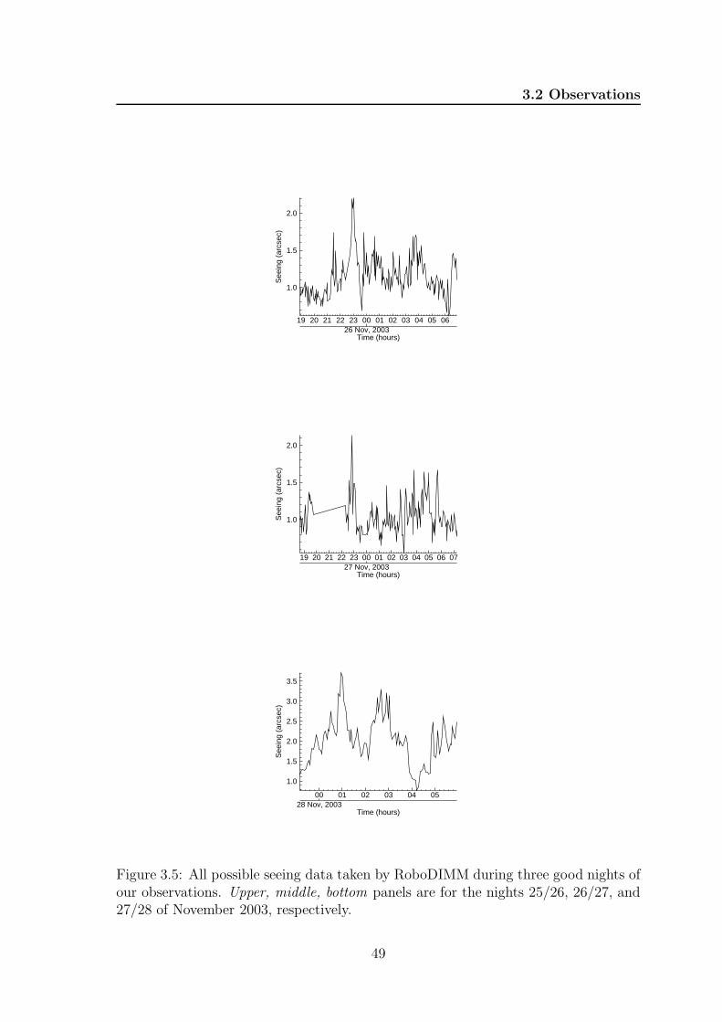
3.2 Observations
See
ing
(arc
sec)
2.0
1.5
1.0
Time (hours)26 Nov, 2003
060504030201002322212019
See
ing
(arc
sec)
2.0
1.5
1.0
Time (hours)27 Nov, 2003
07060504030201002322212019
See
ing
(arc
sec)
3.5
3.0
2.5
2.0
1.5
1.0
Time (hours)28 Nov, 2003
050403020100
Figure 3.5: All possible seeing data taken by RoboDIMM during three good nights ofour observations. Upper, middle, bottom panels are for the nights 25/26, 26/27, and27/28 of November 2003, respectively.
49

3. OPTICAL POLARIMETRY OF THE CRAB PULSAR
24/25 Nov: humidity fluctuates from 100% to 20%, in the morning fog and rain, tempera-
ture changes form ∼ −2 to ∼ 5, some calibration data taken, 27 minutes of
unfiltered Crab observations;
25/26 Nov: clear sky, humidity on the level of 45%, temperature ∼ 6, seeing and trans-
parency changing occasionally (from 2.′′2 to below 1.′′0), RPF and IR filter in-
troduced, channel 3 APD replaced by sky background APD, 8 hours and 15
minutes of Crab pulsar observations;
26/27 Nov: sky partly clouded, high Cirrus clouds, humidity fluctuates from ∼ 45% to
25%, temperature on the level of 5, around midnight wind speed increased to
14 m/s, after midnight seeing below ∼ 1.′′5, 8 hours and 44 minutes of Crab
pulsar observations;
27/28 Nov: very good weather, clear sky, at the beginning of observations humidity on the
level of 20%, around midnight jumps to more than 50%, also the wind speed
increases to 15 m/s, temperature ∼ 5, seeing and transparency changing from
1.′′1 to even more than 3.′′0, 7 hours and 53 minutes of Crab pulsar observations.
Usually one observation set of the Crab pulsar lasted 10 minutes. For brighter
sources it might be shorter because of reaching the data buffer capacity level very
quickly. All together, we had 165 files containing the Crab pulsar observations. How-
ever, three of them, coming from the morning of November 25, were taken without
the RPF and IR filter. Additionally, two of them had very short exposure time, on the
level of tenths of seconds. These five files were not taken for further analysis. For the
remaining 160 files, and all 7 channels of each file, the count rates in 10 seconds bins
were obtained. For good seeing and weather condition, as well as for proper pointing,
we had around 30 − 35% of the total counts in the central fibre, and between 5 and
10% in the background (ring) fibres. When the seeing was high (=bad) then it can
be observed that the count rate for channel 0 goes down, and consequently goes up
for channels 1÷6. We put a threshold on the level of 30% of total counts in channel 0
for the good data selection. By doing so, our end result was 83 files, being equivalent
to 13 hours and 43 minutes of total exposure. 83 selected file names are presented in
Tab. A.1 where, additionally to the file name, the starting data acquisition date and
the UTC time are given.
50

3.3 Data reduction
3.3 Data reduction
3.3.1 Flat field correction
For flat field correction factors of all channels we used two sets of dark sky observations
of the SNR 119.5+10.2 field (CTA-1, α2000 = 00h06.m6, δ2000 = +7247′), i.e. pointing
at α = 00h07m02.s00, δ = +7303′28.′′00. Both observations were taken on November
25. The data acquisition start time of the first file was 21:39:10 and of the second
21:49:13. The exposure time amounted to 600 and 300 seconds for the first and second
observation, respectively. The detected count rates behind the filters fluctuated from
180 Hz for channel 4 up to 240 Hz for channel 6. To obtain the flat field correction
factors we assumed that this value was 1.0 for the central fibre, and we scaled the
count rates of the rest of the fibres to the central one. We binned the data in 10-
seconds intervals, and then calculated the average and uncertainty for each single
channel of the ring fibres. The resulting numbers are shown in Tab. 3.2.
Table 3.2: Fibres flat field correction factorsChannel 0 1 2 3 4 5 6Factor 1.000 1.009 1.074 0.899 0.850 0.956 1.140Uncertainty 0.012 0.013 0.013 0.012 0.011 0.012 0.014
3.3.2 Raw data binning
For each incoming and detected photon the OPTIMA data acquisition system stores
its Time Of Arrival (TOA). A more detailed description of the following steps can
be found in Sec. 3.2.2. By using the OPTIMA system software (Straubmeier 2001)
one can obtain TOAs in units of Julian Date (JD). To assure high time accuracy
two parts of JD are given, the integer and fractional part referring to the day of
observations and to the fractional part of the day, respectively. In order to apply
the rotational model of the pulsar derived from radio observations to our optical
photons, it is required to measure the TOAs in an “inertial observer frame”. Using
the NOT position coordinates (Tab. 3.1), the Crab pulsar coordinates (3.3) and as
planetary ephemeris the JPL DE200 tabulations (Standish 1982) we transformed the
recorded TOAs to the commonly used inertial frame, i.e. to TOAs at the solar system
barycentre.
Parameters of the rotational model of the Crab pulsar (Tab. 3.3) obtained from
the radio observations are regularly, once per month, published by the Jodrell Bank
51

3. OPTICAL POLARIMETRY OF THE CRAB PULSAR
Table 3.3: The Crab pulsar radio ephemeris
Parameter Valueα2000 05h34m31.s972δ2000 +2200′52.′′07Val. range (MJD) 52944–52975t0 (TDB MJD) 52960.000000296ν0 (Hz) 29.8003951530036ν0 (10−10 Hz s−1) -3.73414ν0 (10−20 Hz s−2) 1.18
Observatory pulsar group as a Jodrell Bank Crab Pulsar Monthly Ephemeris1. The
derived radio model is optimised (i.e. it includes the rotational frequency and its
changes, its first and second derivative, as well as, dispersion measure changes, timing
noise effects, glitches and pulsar proper motion) so that it is sufficient to account for
the arrival time of any pulse emitted during the time span of the observations and
predict the arrival times of subsequent photons belonging to these pulses. The model
is based on a Taylor expansion of the angular rotational frequency, ν = 2π/P about
a model value ν0 at some reference epoch t0. The model pulsar phase φ as a function
of barycentric time is thus given by:
φ(t) = φ0 + (t − t0)ν0 +1
2(t − t0)2ν0 +
1
6(t − t0)
3ν0 + . . .
where φ0 is the pulse phase at t0. For each recorded TOA the corresponding pulse
phase was calculated. To obtain a light curve all events are folded according to their
phases with time resolution on the level of 33 µs, that is an equivalent of 1000 bins
per rotational period of the Crab pulsar. The chosen resolution assures a good S/N
ratio even for the phase ranges where the intensity is very low.
We sort the individual events into a 3D data array. The first dimension of this
array is given by the rotational phase of the pulsar. The second dimension is defined
by the polarisation filter phase at the photon’s TOA. This reference position of
the filter is derived from the sequence of Hall sensor signals, which are registered
and timed in the same way as the photon events and stored in a separate channel.
Therefore we can interpolate the position of the polarising filter for any photon event
using the time difference from the preceding and the following Hall sensor signal, i.e.
αRPF (TOA) =tTOA − tbta − tb
· 360,
1see http://www.jb.man.ac.uk/ pulsar/crab.html
52

3.3 Data reduction
where αRPF (TOA) is the RPF angle at which the event was observed, tTOA is the
event time of arrival, whereas tb and ta are the recorded times of the Hall signal sensor
before and after tTOA, respectively. Thus (ta − tb) is nothing else than the period of
rotation of RPF, and then consequently the RPF frequency is νRPF = 1/(ta − tb).
Since during one turn of the RPF all possible polarisation angles are measured two
times, for all values bigger than 180 exactly 180 was subtracted. Thus we have the
second dimension of our 3D array, it spans from 0 to 180 degrees, with 1 intervals.
The third dimension of the data array is assigned to the data channels. We repeated
the pulsar phase and polarisation filter phase calculation for all the events from all
possible channels. The number of channels (seven) defines the length of the 3rd
dimension of the data array. The end result is an array of 1000×180×7 containing the
recorded events, with 1000 and 180 bins for the pulsar and polarisation filter phases
respectively, and 7 channels of measurement. Here we showed a general description
of the first step of the data analysis. However, some irregularities in the rotation
frequency of the RPF have been detected. The RPF state of the art is described in
detail in Sec. 3.3.3.
The obtained light curve of the Crab pulsar and the sinusoidal modulation of
the incoming light due to the RPF are shown in the upper and bottom panels of
Fig. 3.6, respectively. These are the raw data, i.e. without subtracting any nebular
or background light recorded in the central fibre. In both cases two periods are
shown for clarity. For the pulsar light curve (Fig. 3.6, upper) we also indicated its
components: main pulse (MP), inter pulse (IP), non-zero intensity level between
two peaks - bridge, and DC1 region, previously known as the so called ‘off-pulse’
component. For our further analysis we define the DC component as the counts
between phases 0.78−0.84. The Crab pulsar period during the observations (P = 1/ν,
see Tab. 3.3), number of bins used for folding, and the corresponding time resolution
are also given. The amplitude of the modulated polarised light, summed over the
pulsar phase, is at the level of 8%, whereas the maximum is reached at around 119
(Fig. 3.6, bottom).
3.3.3 Rotating polarisation filter characteristics
OPTIMA is configured in such a way that colour filters and/or a rotating linear
polariser (Sec. 3.2.2) can optionally be inserted in front of the incoming beam. In
Sec. 3.3.2 we described the general algorithm for getting the raw data array. Single
1 Direct Current or continuous current, in this case refers to continuous emission componentthat is present along whole rotational phase.
53

3. OPTICAL POLARIMETRY OF THE CRAB PULSAR
0.0 0.5 1.0 1.5 2.0Phase
0.0
0.2
0.4
0.6
0.8
1.0
Nor
mal
ized
Cou
nts
(bef
ore
back
grou
nd s
ubtra
ctio
n)
IP
MP
IP
Bridge BridgeDC DC
Period: 0.033556602 sNo. of Bins: 1000Time Resolution: 33 µs
0 60 120 180 240 300 360Polarization Filter Angle [degree]
0.85
0.90
0.95
1.00
Nor
mal
ized
Cou
nts
(bef
ore
back
grou
nd s
ubtra
ctio
n)
Figure 3.6: Upper : The Crab pulsar light curve obtained from photons recorded bythe central fibre APD. The components of the light curve are indicated as follows:main pulse MP, inter pulse IP, non-zero intensity level between two peaks - bridge,and DC region, previously known as the so called ‘off-pulse’ component in betweenthe 0.78 − 0.84 phase range. Bottom: The sinusoidal modulation of the incomingpolarised light, summed over the pulsar phase. Its amplitude is on the level of 8%,and the maximum is reached at around 119. No background or nebula subtractionhas been applied. In both cases two periods are shown for clarity.
54

3.3 Data reduction
photons are recorded with an accuracy of 4 µs, but to assure the high S/N ratio even
for the low intensity parts of the Crab pulsar light curve we bin the data with 33 µs
resolution. Events are also folded as a function of the RPF phase. To do so we need
the information of the RPF frequency as a function of time. Each single signal coming
from the Hall sensor is recorded in the same way as a regular photon reaching the
fibre bundle and it is stored as a channel 16 event (Sec. 3.2.2). Before calculating
αRPF (TOA) for each event we investigated the polarisation filter behaviour over the
whole observation run. For single observations (corresponding arbitrary file numbers
and the file names containing the observation date can be found in Tab.A.1) we run
a short script that does the following:
1. Checks if there is an inversion in time for succeeding TOAs of the Hall sensor
signal.
2. Calculates the averaged frequency of the filter rotation by using raw and uncor-
rected data (e.g. upper left panels of Fig. 3.7, 3.8). Further used as a threshold
parameter during search for gaps and echos (described in the next algorithm
step).
3. Searches for gaps and echos. During laboratory test runs of the RPF we found
that the tick from a Hall sensor passage is sometimes missing, i.e. the time
between two succeeding ticks is twice as long as average; sometimes we observe
two ticks with a very short time interval, usually below 10 µs. The first case
we call a gap, the second case an echo. Number of occurrences of echos and
gaps as a function of the succeeding good files (files names with corresponding
arbitrary file numbers are given in Tab. A.1) is presented in the upper panel
of the Fig. 3.9. The rate of echos and gaps over the total number of the Hall
sensor signals in each file is shown in the Fig. 3.9, bottom panel.
4. If any gap or echo is found the program corrects for this effects. It interpolates
the missing event or removes the doubled tick. It is instructive to compare in
the left upper and bottom panels of Fig. 3.7 and 3.8 the raw data with the data
corrected by this procedure.
5. Both, short and long time scale variation of the RPF frequency exist (Fig. 3.7,
3.8). For the short one a simple finite impulse response filter procedure as the
boxcar filter is applied. The smoothing function returns a copy of events TOAs
55

3. OPTICAL POLARIMETRY OF THE CRAB PULSAR
smoothed with a boxcar average of the specified width. The algorithm is:
SMOOTHED TOARPF,i =
1w
∑w−1j=0 TOARPF,i+j−w/2, i = (w−1)
2, . . . , N − (w+1)
2
TOARPF,i, otherwise,
where N is the recorded number of RPF TOAs, and w is the width of the
smoothing window. Usually w was on the level of 10 bins, thus taking the
averaged RFP frequency gives us the smoothing window on the time scale of 3
seconds. The long time scale variations of the RPF frequency have to be kept
as they were.
6. The average RPF frequency during single observations, with its standard devia-
tion σ, over the whole observation is calculated (Fig. 3.10). The RPF frequency
averaged over the whole observational time span amounts to 3.4 Hz, whereas
the averaged RPF frequency of a single 10 minutes observational set varies from
2.85 Hz up to 3.75 Hz. Moreover, it might be seen that the deviations σ also
differ. They strongly depend on the long time scales variation of the RPF, see
e.g. bottom left panels of the Fig. 3.7 and 3.8.
7. Smoothed TOAs of the RPF events are stored in the file and later are used to
calculate for each single event the αRPF (TOA) introduce in Sec. 3.3.2 .
56

3.3
Data
reductio
n
Crab-IR+Pol_26Nov2003 (27-11-2003 03-28-52)_(Channel_16)
0 500 1000 1500 2000Polarization Filter Rotation Number
0.2
0.3
0.4
0.5
0.6
∆ TO
A [s
]
Echos: 0, Gaps: 6
0 500 1000 1500 2000Polarization Filter Rotation Number
0.265
0.270
0.275
0.280
0.285
∆ TO
A [s
]
SMOOTHING, No. of Bins: 10 --> Time: 3 s
0 500 1000 1500 2000Polarization Filter Rotation Number
0.270
0.272
0.274
0.276
0.278
0.280
0.282
0.284
∆ TO
A [s
]
Exposure Time: 600 s
0 500 1000 1500 2000Polarization Filter Rotation Number
-0.006
-0.004
-0.002
0.000
0.002
0.004
0.006
TO
AS
MO
OT
HE
D -
TO
AO
BS
ER
VE
D [s
]
Figure 3.7: Example of the RPF behaviour during one 10 minutes observation. Upper left: raw data time intervals betweentwo succeeding RPF TOAs. File name is given in the title. Solid line represents the average value, whereas the dashed linesshow 5 σ of the average value. Bottom left: the same as above, but after correcting for the bad events occurrence, i.e. gapsand echos, for the detailed description see Sec. 3.3.3. Numbers of bad events are given in the title. Upper right: time intervalbetween two succeeding RPF TOAs after applying the smoothing procedure. The width of the smoothing window is given inthe title. Bottom right: residuals between the smoothed and observed RPF TOAs. Dashed lines show 1 σ standard deviationof the expected normal distribution. Additionally exposure time is given in the title.
57

3.
OP
TIC
AL
PO
LA
RIM
ET
RY
OF
TH
EC
RA
BP
ULSA
RCrab-IR+Pol_25Nov2003 (26-11-2003 04-43-30)_(Channel_16)
0 500 1000 1500Polarization Filter Rotation Number
0.0
0.2
0.4
0.6
0.8
∆ TO
A [s
]
Echos: 2, Gaps: 1
0 500 1000 1500Polarization Filter Rotation Number
0.31
0.32
0.33
0.34
0.35
∆ TO
A [s
]
SMOOTHING, No. of Bins: 9 --> Time: 3 s
0 500 1000 1500Polarization Filter Rotation Number
0.315
0.320
0.325
0.330
0.335
0.340
0.345
∆ TO
A [s
]
Exposure Time: 600 s
0 500 1000 1500Polarization Filter Rotation Number
-0.006
-0.004
-0.002
0.000
0.002
0.004
0.006
0.008
TO
AS
MO
OT
HE
D -
TO
AO
BS
ER
VE
D [s
]
Figure 3.8: The same as for the Fig. 3.8. Some other 10 minutes observation data are shown as an example of the RPFbehaviour, suffering from both of the bad timing events, i.e. gaps and echos.
58

3.3 Data reduction
It is not clear what gives rise to the long time scale variation of the RPF frequency.
It might be caused e.g. by a rather unstable voltage supply of the motor, or by
different position of the OPTIMA instrument with respect to the ground during
the observing night, as well as by changes of the belt resistance with the outdoor
temperature. We corrected incoming RPF TOAs for the short time scale variation,
but still there is an evidence that we have some problems with the angular speed over
single rotation of the filter. Quite likely, the speed of the RPF during one rotation
was not perfectly constant: let’s recall that the small wheel getting the momentum
from the motor needs three and 1/3 rotations for one turn of the polarisation filter
wheel. If there are any changes in the voltage given to the motor, then they will
cause changes in the angular speed of the small wheel, and in consequence also in
the rotational speed of the main wheel. Additionally, we might be observing some
reflection of starlight from the non-dark parts of the RPF (see Fig. 3.3). This light
comes from the stars seen by the CCD mirror. So far these effects have not been
corrected. However none of these small systematic effects are synchronous to the
Crab pulsar rotation. Their effect on the astronomical result is therefore limited to a
possible smearing of any details. The sharpness of resolution of the Crab polarisation
confirms, however, that the systematics of the RPF are of minor importance.
59

3. OPTICAL POLARIMETRY OF THE CRAB PULSAR
0 20 40 60 80Arbitrary Data File Number
0
1
2
3
4
5
6
Num
ber o
f ech
os [*
] and
gap
s [+
]
0 20 40 60 80Arbitrary Data File Number
0.00
0.05
0.10
0.15
0.20
0.25
Per
cent
age
of e
chos
(gre
en) a
nd g
aps
(blu
e) [%
]
Figure 3.9: Upper : Number of occurrences of the echos and gaps as a function of thesucceeding good files (selected file names with corresponding arbitrary file numbersare given in Tab. A.1). Bottom: Rate of the echos and gaps over the total numberof Hall sensor signals in each file is shown. For our data set we have never had ina single file more than 0.28% of bad events over the total number of RPF TOAs inthat file.
60

3.3 Data reduction
0 20 40 60 80Arbitrary Data File Number
3.0
3.2
3.4
3.6
Pol
ariz
atio
n Fi
lter F
requ
ency
[Hz]
3.403 [Hz]
0 20 40 60 80Arbitrary Data File Number
350
400
450
500
550
600
Exp
osur
e Ti
me
[s]
Total Exposure Time: 13.7215 hours
Figure 3.10: Upper : The average RPF frequency with its standard deviation as afunction of the succeeding good files (selected files names with corresponding arbitraryfile numbers are given in Tab. A.1). Averaged over the whole observational time spanthe RPF frequency is 3.4 Hz, whereas for single files the RPF frequency varies from2.85 Hz up to 3.75 Hz. The standard deviations differ very much as well. Theystrongly depend on the long time scales variation of the RPF frequency. Bottom:Exposure time of the selected data files. For 81 files the exposure is about 600seconds; only two files have exposure time shorter than 500 seconds. Total exposuretime amounts to ∼ 14 hours. 61

3. OPTICAL POLARIMETRY OF THE CRAB PULSAR
3.3.4 Polarisation data analysis
Accurate derivation of polarisation information about any highly non-thermal astro-
nomical object (pulsars in particular) is an essential step in the investigation of its
underlying physical processes. Considering astronomical objects in general, the de-
gree of polarisation is often low, a few percent is a typical value, though both much
higher and lower values do occur. A polarimetric measurement is basically that of
the ratio of the small difference between two signals to their sum. Different meth-
ods have been devised to measure this small difference without systematic bias or
drift errors; but detector noise or photon noise of the signal itself is always present.
To minimise the contribution of the photometric noise considerable observing time
on a large telescope is generally required. Use of large area detectors for imaging
and spectroscopy has become commonplace, and frequently such instruments offer a
polarisation capability. Processing of polarimetric data, however, is nontrivial, espe-
cially when the polarimeter is far from ideal. On the other hand we have to remember
that sufficiently accurate polarimetry provides an insight that other methods can not
give. Therefore, it is worth to put an effort in performing polarisation observations,
analysing polarimetric data, but also in developing polarimetric instrumentation.
Hereafter, we present step-by-step polarisation data analysis by using the method-
ology described by Sparks & Axon (1999). The rotating polarisation filter inside the
OPTIMA instrument provides us with polarimetric data that comprise a series of
“images” of an object taken through 180 sets of linear polarisers. Let us remind that
we chose one degree resolution of the RPF data, therefore we had 180 polarisers. A
single polariser is not a 100% perfect polariser, but its characteristics are well estab-
lished, and this is essential for the chosen data analysis method. From an input data
set of 180 intensities I (measured in counts) and their errors (σI =√
I), assumed in-
dependent between observations, corresponding to a set of observations through these
180 polarisers (identical but not perfect) we derive the Stokes parameters, following
the case of n polarisers after Sparks & Axon (1999), .
Linearly polarised light
A monochromatic linearly polarised electromagnetic wave in vacuum is the simplest
concept of polarised light. It has a transverse electric field vector with constant
orientation, its strength at any point in space varying strictly sinusoidally with time.
The duration of this wave is infinite; it has constant amplitude and frequency at all
times. The wave that is 100% polarised, but its amplitude and phase is allowed to
62

3.3 Data reduction
vary slowly and often randomly, is a quasi-monochromatic wave. The faster these
variations are, the broader the range of frequencies contained within the wave will
be. Fully or 100% linearly polarised polychromatic radiation is a superposition of
quasi-monochromatic waves of many different frequencies; there is usually no stable
phase relation between the electromagnetic field at different frequencies. There is
now no single dominant frequency, amplitude or phase, just a unique orientation of
the otherwise often randomly oscillating electric field vector. Random in this case
means random within the constraints of the mean flow of radiant energy and of the
spectral bandwidth.
It is a matter of convenience to clearly define the dividing line between quasi-
monochromatic and polychromatic radiation. The wider the bandwidth (the faster
the modulation) the less useful is to regard the polychromatic radiation as a sine wave
modulated in phase and amplitude. In this case the polychromatic description is more
appropriate. When fractional bandwidth is small enough that one can neglect any
frequency dependence of wave amplitude, phase, receiver gain, refractive index etc.,
one uses a quasi-monochromatic description, whereas when functional dependence on
frequency is important, a polychromatic description is needed.
For our purpose we assume that we observe a quasi-monochromatic radiation,
i.e. we do not take into account the possibility that within our bandwidth there is
any frequency dependence of a sine wave modulation. Most probably it is not true,
but so far we were not able to correct for this effect. It could have been done by
using not only the polarisation filter, but also one out of three colour filters at that
time. However, this combination would give us much lower S/N ratio. Moreover,
spectral characteristics of the pulsar radiation change with its rotational phase (see
e.g. integrated and phase resolved spectral power laws from photometric analysis
performed by Golden et al. (2000a)).
Linearly polarised light requires measurement of three quantities to fully charac-
terise it. There are various ways of expressing it. The most common one involves
the total intensity of the light I, the degree of polarisation p, and the position angle
θ. An “intermediate” stage between the input data and the solution of polarisation
quantities are the Stokes parameters (I, Q, U) that are related through:
Q = Ip cos 2θ, U = Ip sin 2θ, (3.1)
or the other way around,
p =(Q2 + U2)1/2
I, θ =
1
2arctan
(
U
Q
)
. (3.2)
63

3. OPTICAL POLARIMETRY OF THE CRAB PULSAR
These quantities describe all intrinsic properties of the linearly polarised radiation of
the source. Here we would like to underline that they should not be confused with
the properties of the polarising elements of the polarimeter, which in our case are the
properties of the measured intensities in each one of the degree intervals of the RPF,
i.e. in each of 180 polarisers.
Polarising element characteristics
A linearly polarising element requires three quantities to characterise its behaviour
or response fully. These are:
- its efficiency as a polariser (hereafter ε), i.e. the ability to reject and accept
polarised light of perpendicular and parallel orientations,
- its overall throughput (hereafter t), in particular to unpolarised light,
- the position angle of the polariser (hereafter φ).
There are a variety of conventions commonly used to present these quantities (Maz-
zuca et al. 1998). Here, we adopt the convention that the output intensity of a beam
with input Stokes parameters (I, Q, U) passing through a polarising element is given
by
Ik =1
2tk[I + εk(cos 2φkQ + sin 2φkU)] (3.3)
where the subscript k anticipates that the polarising element is the k-th of a series, t
is related to the throughput to unpolarised light, ε is the efficiency of the polariser,
and φ is the position angle of the polariser. In this formalism three perfect polarisers
at optimal orientation would have tk = 1, εk = 1, ( φ1, φ2, φ3) = (0, 60, 120), in
the contrary to a perfectly bad polariser that would have tk = 2, εk = 0, and the
φk values can be anything (since ε is zero). In the case of n polarisers of arbitrary
characteristics a direct observation of the target without any polarising element in
the beam may be used as part of the observing sequence. Then the formula above
will allow this additional observation to form part of the derivation of polarisation
quantities to maximise the obtainable S/N.
We assume that we have made a set of n = 180 observations of our target, each
using a polarising element of well known, truly exactly the same, characteristics. Our
case is the case of repeating observations with the same polariser, OPTIMA RPF.
One needs at least three observations to get the solution for the three unknowns in
the description of the polarisation of the incoming light. The measured intensity Ik
64

3.3 Data reduction
through the kth polariser is related to the Stokes parameters and polariser character-
istics by Eq. (3.3). An uncertainty associated with the Ik measurement is assumed
to follow Poisson distribution and it is denoted as σk, thus σk =√
Ik. We adopted
the Sparks & Axon approach to the n polarisers case, but firstly the solution for the
case of the required minimum number of polarisers, i.e. three, is presented.
The case of three polarisers
The minimum number of polarisation observations required to determine the three
unknowns represented by the Stokes parameters is obviously three. Equation (3.3)
above with k in the range 1–3 gives three equations for the three unknowns, (I, Q,
U)
I1 =1
2t1[I + ε1(cos 2φ1Q + sin 2φ1U)],
I2 =1
2t2[I + ε2(cos 2φ2Q + sin 2φ2U)],
I3 =1
2t3[I + ε3(cos 2φ3Q + sin 2φ3U)].
This straightforward linear system may be explicitly solved to yield
(I, Q, U) = A
I1
I2
I3
(3.4)
or to introduce a minor simplification
(I, Q, U) = B
I?1
I?2
I?3
(3.5)
where I?k = Ik/(0.5tk) (i.e., the matrix A is the matrix B with rows divided by 0.5tk)
and the matrix B is given by
B =
ε2ε3 sin(2φ3 − 2φ2) ε1ε3 sin(2φ1 − 2φ3) ε1ε2 sin(2φ2 − 2φ1)ε2 sin 2φ2 − ε3 sin 2φ3 ε3 sin 2φ3 − ε1 sin 2φ1 ε1 sin 2φ1 − ε2 sin 2φ2
ε3 cos 2φ3 − ε2 cos 2φ2 ε1 cos 2φ1 − ε3 cos 2φ3 ε2 cos 2φ2 − ε1 cos 2φ1
/Ω
(3.6)
where
Ω = ε1ε2 sin(2φ2 − 2φ1) + ε2ε3 sin(2φ3 − 2φ2) + ε1ε3 sin(2φ1 − 2φ3). (3.7)
For our data analysis we used a similar method, but adapted for n polarisers. It is
described below. Having high efficiency, ε = 0.998, but low transmittance, t = 0.32,
65

3. OPTICAL POLARIMETRY OF THE CRAB PULSAR
our rotating polarisation filter does not have the characteristics of a perfect polariser.
However, with appropriate characterisation it may still be used with excellent effect.
For these purpose we use all available data, i.e. 180 polarisers; we then obtain optimal
orientation.
The case of n polarisers
An analogous solution can be derived for the case of n (n > 3) polarisers, keeping in
mind that we still have only three unknowns. This means that the equations are over
determined. Sparks & Axon (1999) adopted a maximum likelihood approach, which
is equivalent to a least-squares minimisation.
Let us assume that the true underlying values of the Stokes parameters of the
target are (I, Q, U). Then we would expect to observe a mean intensity through the
kth polariser of I ′k as in Eq. (3.3):
I ′k =
1
2tk[I + εk(cos 2φkQ + sin 2φkU)]. (3.8)
Hence the likelihood of observing a particular value Ik, given an underlying mean of
I ′k, is
ρk =1√
2πσk
e−(Ik−I′k)2/2σ2
k ,
and hence the likelihood of observing a set of n values Ik is
ρ = ρ1ρ2 . . . ρn, ρ = ρ0 exp
[
−(I1 − I ′1)2
2σ21
− (I2 − I ′2)2
2σ22
− (I3 − I ′3)
2
2σ23
− . . .
]
,
where ρ0 is a constant.
Maximising the likelihood function ρ is equivalent to minimising the absolute value
of the exponent, which is a sum of normalised deviations from the mean value. With
this “least-squares” estimate, the problem reduces to minimise
χ2 =1
2
∑
k
(Ik − I ′k)2
σ2k
. (3.9)
The values of I ′k can be substituted into Eq. (3.9) from Eq. (3.8), and minimisation
of χ2 is obtained by taking partial derivatives with respect to each of I, Q, U in turn
66

3.3 Data reduction
and equating to zero. Algebraic manipulation leads to a set of three equations
∑ Iktkσ2
k
=1
2
∑ t2kσ2
k
I +1
2
∑ t2kεk cos 2φk
σ2k
Q +1
2
∑ t2kεk sin 2φk
σ2k
U,
∑ Iktkεk cos 2φk
σ2k
=1
2
∑ t2kεk cos 2φk
σ2k
I +1
2
∑ t2kε2k cos2 2φk
σ2k
Q+
+1
2
∑ t2kε2k sin 2φk cos 2φk
σ2k
U, (3.10)
∑ Iktkεk sin 2φk
σ2k
=1
2
∑ t2kεk sin 2φk
σ2k
I +1
2
∑ t2kε2k sin 2φk cos 2φk
σ2k
Q+
+1
2
∑ t2kε2k sin2 2φk
σ2k
U,
where∑
denotes a sum over index k of the n polariser observations. This means
that again we have a set of three equations and three unknowns. It is very similar
in form to the set of three equations for the three-polariser case solved above and, in
fact, is identical if we define a set of “effective three-polariser characteristics” using
these weighted sums.
That is, the three terms on the left hand side of Eqs. (3.10) can be used as (I1, I2,
I3) in Eq. (3.3). We label these new parameters as I ′′k , to get the new three-component
vector of effective measurements:
I ′′1 =
∑ Iktkσ2
k
, I ′′2 =
∑ Iktkεk cos 2φk
σ2k
, I ′′3 =
∑ Iktkεk sin 2φk
σ2k
. (3.11)
The error estimate for each measured intensity (=counts) is based on Gaussian
statistics; therefore Ik = σ2k and the corresponding factors reduce to unity. The results
of calculating the effective intensity components I ′′1 , I ′′
2 and I ′′3 are shown in Fig. 3.11.
In our case these values are constant. I ′′1 is just a sum over the same 180 polarisers
with the same throughput to unpolarised light, i.e. t = 0.32. Therefore we get:
I ′′1 = 180 × 0.32 = 57.6. Whereas, I ′′
2 = 180tε∑
cos 2φk and I ′′s = 180tε
∑
sin 2φk,
where∑
denotes a sum over index k of the 180 polarisers. Knowing that ε = 0.998
and the integrals of cos 2φk and sin 2φk over the range from 0 to 180 we expect
I ′′2 ∼ I ′′
1
∑
cos 2φk and I ′′3 ∼ I ′′
1
∑
sin 2φk, within available numerical precision, to be
very close to zero.
Similarly, we can define a three-component vector of effective transmittances:
t′′1 =∑ t2k
σ2k
, t′′2 =∑ t2kεk cos 2φk
σ2k
, t′′3 =∑ t2kεk sin 2φk
σ2k
. (3.12)
In Fig. 3.12 three components of the vector of effective transmittance, t′′1, t′′2 and t′′3
(Eqs. (3.12)), as a function of the pulsar rotation are presented.
67
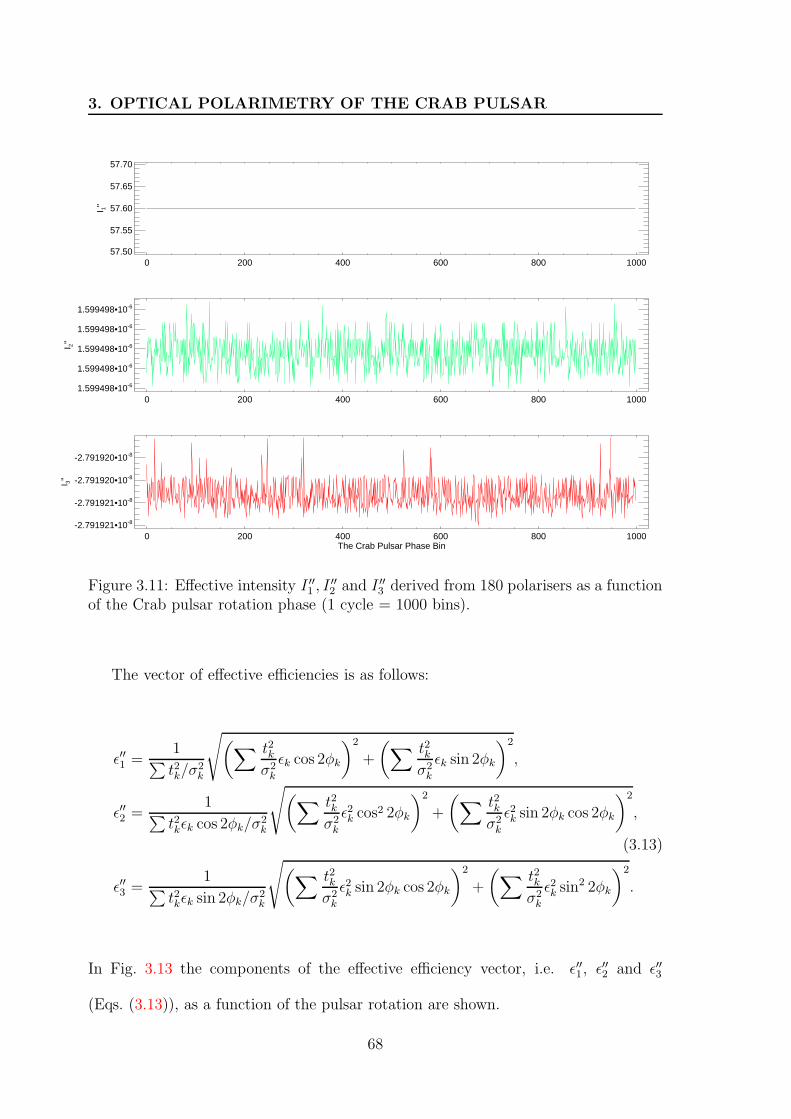
3. OPTICAL POLARIMETRY OF THE CRAB PULSAR
0 200 400 600 800 100057.50
57.55
57.60
57.65
57.70
I 1"
0 200 400 600 800 10001.599498•10-6
1.599498•10-6
1.599498•10-6
1.599498•10-6
1.599498•10-6
I 2"
0 200 400 600 800 1000The Crab Pulsar Phase Bin
-2.791921•10-8
-2.791921•10-8
-2.791920•10-8
-2.791920•10-8
I 3"
Figure 3.11: Effective intensity I ′′1 , I ′′
2 and I ′′3 derived from 180 polarisers as a function
of the Crab pulsar rotation phase (1 cycle = 1000 bins).
The vector of effective efficiencies is as follows:
ε′′1 =1
∑
t2k/σ2k
√
(
∑ t2kσ2
k
εk cos 2φk
)2
+
(
∑ t2kσ2
k
εk sin 2φk
)2
,
ε′′2 =1
∑
t2kεk cos 2φk/σ2k
√
(
∑ t2kσ2
k
ε2k cos2 2φk
)2
+
(
∑ t2kσ2
k
ε2k sin 2φk cos 2φk
)2
,
(3.13)
ε′′3 =1
∑
t2kεk sin 2φk/σ2k
√
(
∑ t2kσ2
k
ε2k sin 2φk cos 2φk
)2
+
(
∑ t2kσ2
k
ε2k sin2 2φk
)2
.
In Fig. 3.13 the components of the effective efficiency vector, i.e. ε′′1, ε′′2 and ε′′3
(Eqs. (3.13)), as a function of the pulsar rotation are shown.
68

3.3 Data reduction
0 200 400 600 800 1000
0.01
0.02
0.03
0.04
0.05
t 1"
0 200 400 600 800 1000
0.00000.00020.0004
0.00060.00080.0010
0.0012
t 2"
0 200 400 600 800 1000The Crab Pulsar Phase Bin
0.000
0.001
0.002
0.003
0.004
t 3"
Figure 3.12: Effective transmittance t′′1, t′′2 and t′′3 derived from 180 polarisers as a
function of the Crab pulsar rotation phase (1 cycle = 1000 bins).
Finally a vector of effective “position angles” is defined as:
φ′′1 =
1
2arctan
(
∑ t2kσ2
k
εk sin 2φk
/
∑ t2kσ2
k
εk cos 2φk
)
,
φ′′2 =
1
2arctan
(
∑ t2kσ2
k
ε2k sin 2φk cos 2φk
/
∑ t2kσ2
k
ε2k cos2 2φk
)
, (3.14)
φ′′3 =
1
2arctan
(
∑ t2kσ2
k
ε2k sin2 2φk
/
∑ t2kσ2
k
ε2k sin 2φk cos 2φk
)
.
The results of calculating the effective position angle components φ′′1, φ
′′2 and φ′′
3
(Eqs. (3.14)) are shown in the Fig. 3.14.
By making these substitutions, the solution given by Eq. (3.5) and Eq. (3.6) can
be used immediately. In this way we obtained the Stokes parameters (Fig. 3.15).
That is, a set of observations with n polarisers can be made equivalent to a set of
observations through three polarisers.
In the actual case of n = 3, it can also be shown that the maximum likelihood
69

3. OPTICAL POLARIMETRY OF THE CRAB PULSAR
0 200 400 600 800 1000
0.02
0.03
0.04
0.05
0.06
0.07
0.08
ε 1"
0 200 400 600 800 1000
-5.0•103
0
5.0•103
1.0•104
1.5•104
2.0•104
2.5•104
ε 2"
x 100
0 200 400 600 800 1000The Crab Pulsar Phase Bin
0
1000
2000
3000
ε 3"
x 100
Figure 3.13: Effective efficiency ε′′1, ε′′2 and ε′′3 derived from 180 polarisers as a function
of the Crab pulsar rotation phase (1 cycle = 1000 bins).
or least-squares solution is identical to the direct matrix inversion used for the three-
polariser case.
70

3.3 Data reduction
0 200 400 600 800 1000-0.20.00.20.40.60.81.0
φ 1"
0 200 400 600 800 1000
-0.002
0.000
0.002
0.004
0.006
φ 2"
0 200 400 600 800 1000The Crab Pulsar Phase Bin
0.780
0.782
0.784
0.786
φ 3"
Figure 3.14: Effective position angle φ′′1, φ
′′2 and φ′′
3 derived from 180 polarisers as afunction of the Crab pulsar rotation phase (1 cycle = 1000 bins).
71

3. OPTICAL POLARIMETRY OF THE CRAB PULSAR
0 200 400 600 800 1000
5.0•103
1.0•104
1.5•104
2.0•104
2.5•104
3.0•104
I
0 200 400 600 800 1000
-2500
-2000
-1500
-1000
-500
0
Q
0 200 400 600 800 1000The Crab Pulsar Phase Bin
-1500
-1000
-500
0
500
U
0 200 400 600 800 10000
20
40
60
80
100
Nor
mal
ised
I
0 200 400 600 800 1000
-8
-6
-4
-2
0
Nor
mal
ised
Q
0 200 400 600 800 1000The Crab Pulsar Phase Bin
-6
-4
-2
0
Nor
mal
ised
U
Figure 3.15: Raw (upper three panels) and normalised (bottom three panels) Stokesparameters I, Q, U derived from 180 polarisers as a function of the Crab pulsarrotation phase (1 cycle = 1000 bins). Normalisation was such that I = 100 at themaximum, and Q and U are normalised to I. These values corresponds to the valuesshown on the QU plane in the Fig. 3.19.
72

3.3 Data reduction
3.3.5 The HST polarisation standards
In order to understand the intrinsic polarisation and the response of the instrument
to known polarised stars we have performed observations of such reference stars
(Tab. 3.4). Since OPTIMA is very sensitive and limited in its capacity for data
acquisition at a high rate (count rate above 37 kHz, Muhlegger (2006)) we selected
three of the weakest stars from the list of Turnshek et al. (1990): two polarisation
standards, and one photometric standard (see Tab. 3.4). The first one of two polari-
sation standard stars is highly polarised, on the level of 6%, whereas the second star
has a very low polarisation degree of ∼1 . Unfortunately for our measurements both
stars are quite bright for the OPTIMA instrument. Therefore, we also performed op-
tical polarisation measurements of a dimmer star, i.e. a photometric standard from
Turnshek et al. (1990) list, expecting its light not to be polarised.
Table 3.4: HST polarisation and photometric standards (Turnshek et al. 1990)
Name FK5 2000.0 Coordinates Spectral Type CommentsHST Polarisation Standards
BD+64 106 00h 57m 36.s70 B1V V = 10.34+64 51′ 34.′′9 P: 5.65 ± 0.053%
θ: 96.8
G191B2B 05h 05m 30.s61 WD V = 11.79+52 49′ 51.′′9 P: 0.09 ± 0.048%
HST Photometric StandardsGD50 03h 48m 50.s20 WD V = 14.06
−00 58′ 31.′′2
We have performed observations of the HST polarisation standard BD+64 106 two
times during our observational campaign for 4.5 and 6.17 minutes on November 25th
and 27th, respectively (see Tab. 3.5, left side). In both cases the observing conditions
were very different, thus the results differ as well. Hereafter, we would like to discuss
them in details. In between 22:06:45 and 22:12:56 of Nov 25th the average seeing was
on the level of 1.′′27 (RoboDIMM measurements, see Fig. 3.5, upper panel), whereas
for the time span between 21:33 and 21:40 of Nov 27th no information about the
seeing conditions were provided by the RoboDIMM telescope. At the beginning of
the night the weather was very good. But later, during less than two hours, between
20:00 and 22:00, the humidity changed from 20 to almost 60%, and the wind speed
increased up to 15 m/s. Therefore the seeing was probably larger than during the
first observations, likely more than 2.′′0. This dissimilarity in the seeing values causes
different count rates in the central and ring fibres. During the Nov 25th count rate
73

3. OPTICAL POLARIMETRY OF THE CRAB PULSAR
in channel 0 was on the level of 1.9 × 10⁵ Hz, and in the ring fibres . 2.0 × 10⁴ Hz,
while during Nov 27th we had 1.5×10⁵ Hz and . 5.0×10⁴ Hz for channel 0 and ring
fibres, respectively. Summarising, it is important to notice that for all observations
the central channel was saturated, i.e. the count rates were well above the saturation
threshold, i.e. 37 kHz. For the second set of data (Nov 27th) it might have happened
that some of the ring fibres were also saturated. The most saturated channels were 1
and 6. The values of the polarisation degree and the position angle for all channels
and for all sets of observations are gathered in the right side of the Tab. 3.5. It is
important to notice that, even if the central fibre was suffering pile-up, the calculated
position angle for each single observation of BD+64 104 is pretty constant. This
is caused by the fact that the position angle, being nothing else than the phase of
the maximum of the modulated incoming light, is not (under the condition that any
modulation is observed) so strongly dependent on the pile-up effect. Saturation is
important in the case of calculating the polarisation degree, which is the amplitude
of the measured light modulation. If the channel is saturated then the values of
the polarisation degree are not reliable. We can observe this by comparing results
in Tab. 3.5. For the central fibre there is significant difference in the polarisation
degree for the first and second sets of data. When seeing was higher the light from
the observed very bright star was more smoothly distributed among all channels,
therefore an increase of p in the central fibre is observed. Seeing conditions, being an
equivalent to the count rates, did not affect significantly the measured values of p in
the ring fibres. Only in the case of channel 1 the polarisation degree is much smaller
during the Nov 27 observations than Nov 25. This is strongly connected with the fact
that, during the second observation, this channel, among all of the ring channels, was
the most saturated one.
Taking into account the resulting θ and p (Tab. 3.7) of the HST polarisation
standard BD+64 104 (being a very bright star for the OPTIMA instrument) we can
conclude that for the purpose of calibrating the north direction of our instrument it is
safe and valid to use values of the polarisation angle from the central fibre (Tab. 3.5,
marked with the grey background). The averaged value of θBD+64104 amounts to
96.74 ± 0.37 (see Tab. 3.7). From these calibration observations we learned that we
had to shift the RPF angles by 92. The angles θ given here and hereafter in text and
in tables are the E−vector position angles relative to celestial north (N to E). The
amplitude of sinusoidally modulated intensity of the incoming light is not correct in
the case of saturation. Thus, probably the best estimate of the polarisation degree of
BD+64 104 comes from the sum of the light detected in the ring fibres. The obtained
74

3.3 Data reduction
value, 4.72 ± 0.30%, is somehow smaller than the value in the measured by the HST
table (5.65 ± 0.053%), but one has to remember that our value is obtained from the
ring fibres measuring ”background” around the star. Because the star is very bright,
and seeing was more than 1.′′0, the light of the star was scattered into the ring fibres.
In this case bad seeing (high value) is an advantage, because it naturally defocuses
our target.
We also performed observations of the unpolarised HST standard, i.e. G191B2B
(Tab. 3.4). Data for this target were taken on Nov 26 21:30 for about 10 minutes
with seeing being on the level of 1.′′0. We found a very small polarisation degree
for this star, as expected, and thus the position angle has little meaning. During
observations the count rate was on the level of 1.5 × 10⁵ Hz and < 4 × 10⁴ Hz in the
central and ring fibres, respectively. Even though the channel 0 was saturated our
result, 0.05 ± 0.02% (Tab. 3.7), is in a good agreement with the value 0.09 ± 0.048%
obtained by Turnshek et al. (1990). The averaged value from the background fibres
is higher. It amounts to 0.33± 0.02%, and is probably partly caused by the polarised
sky background.
For the purpose of the instrument calibration we also chose from the Turnshek
et al. (1990) atlas of Hubble Space Telescope photometric, spectroscopic, and po-
larimetric calibration objects a star with brightness that should assure count rates
lower that the pile-up threshold. GD50 (Tab. 3.4) is a photometric standard, thus
we expect its light not to be polarised. Observations of this target were performed
on November the 27th at 21:52 with recorded count rate in the central channel of
(1.0− 1.5)× 104 Hz and in the ring channels < 1000 Hz. Results of pGD50 are shown
in the Tab. 3.6, file A. The source had polarisation degree below 1 (measured in
the central fibre), whereas the measured p within the ring fibres was much greater.
These values correspond to the sky background polarisation. However, the sky back-
ground could have been more highly polarised. The contribution of the night sky to
the observed count rates was on the level of one quarter in each fibre only, i.e. the
background ring fibres were contaminated by the source. Thus, the signal measured
in the ring fibres was most probably depolarised and could have higher polarisation
degree in reality.
75

3.
OP
TIC
AL
PO
LA
RIM
ET
RY
OF
TH
EC
RA
BP
ULSA
RTable 3.5: Measurements of the HST polarisation standard BD+64 104 (the files from 1 to 5). Table consists of two parts: theleft side part gives information about the arbitrary file number, date and time of observation and length of exposure, whereasthe right side part gives p (above) and θ (below) as a function of single observation and channel. Additionally, last raw (assignedas “1 ÷ 6” ) shows p and θ values obtained as a function of different data sets after averaging the Stokes parameters from allring channels. Columns titled “1 ÷ 2” “3 ÷ 5” and “1 ÷ 5” give the p and θ values for single channel, as well as for sum of thering fibres (last raw), obtained after summing all existing data of the target from Nov 25th, Nov 27th and both days together,respectively.
File Date and Time of Observations Exposure [s]
1 25 Nov 2003 22:07:01 140
2 25 Nov 2003 22:09:46 130
3 27 Nov 2003 21:33:35 110
4 27 Nov 2003 21:36:08 120
5 27 Nov 2003 21:38:34 120
File 1 2 3 4 5 1÷2 3÷5 1÷5
Channel
0 p 1.30 1.35 1.98 1.86 1.67 1.33 1.83 1.59
θ 96.6 96.8 96.2 96.9 97.2 96.7 96.8 96.7
1 p 4.57 4.64 3.71 3.60 4.21 4.60 3.81 3.87θ 100.3 96.6 98.0 96.5 98.3 98.4 98.0 98.0
2 p 5.16 5.17 4.59 4.84 5.57 5.16 4.99 5.04θ 96.0 94.7 98.0 96.8 96.8 95.3 97.2 96.6
3 p 5.38 5.16 5.49 5.08 5.04 5.25 5.20 5.22θ 94.3 92.9 95.5 95.9 97.4 93.5 96.2 94.6
4 p 4.67 4.34 4.14 4.98 4.27 4.49 4.46 4.48θ 99.1 98.6 98.5 100.5 103.5 98.8 100.7 99.5
5 p 5.51 5.26 5.53 5.58 5.38 5.38 5.50 5.46θ 96.7 94.3 97.9 96.2 97.1 95.5 97.0 96.5
6 p 4.62 5.00 5.06 4.52 4.80 4.81 4.80 4.79θ 98.6 98.7 93.6 93.6 91.7 98.6 93.0 93.7
1÷6 p 5.06 4.95 4.47 4.37 4.73 5.00 4.51 4.63θ 96.7 95.1 96.8 95.8 96.4 95.8 96.3 96.2
76

3.3
Data
reductio
n
Table 3.6: Measurements of the HST polarisation standard G191B2B (files from 1 to 4) and the HST photometric standardGD50 (file A). Table consists of two parts: the left side part gives information about the arbitrary file number, date and timeof observation and length of exposure, whereas the right side part gives p as a function of single observation and channel.Moreover, last raw (assigned as “1 ÷ 6” ) shows p value obtained as a function of different data sets after averaging the Stokesparameters from all ring channels. Column titled “1 ÷ 4” gives the p value for single channel, as well as for sum of the ringfibres (last row), obtained after summing all existing data of G191B2B from Nov 26th. For GD50 we had only one 10 minutesobservation.
File Date and Time of Observation Exposure [s]
1 26 Nov 2003 21:33:08 160
2 26 Nov 2003 21:36:22 150
3 26 Nov 2003 21:41:01 130
4 26 Nov 2003 21:43:53 130
A 27 Nov 2003 21:52:17 590
File. 1 2 3 4 1÷4 A
Channel
0 p 0.04 0.07 0.03 0.06 0.03 0.08
1 p 0.37 0.48 0.47 0.21 0.31 0.30
2 p 0.75 0.41 0.65 0.85 0.62 0.44
3 p 0.84 0.46 0.80 0.72 0.63 0.61
4 p 0.30 0.66 0.69 0.47 0.43 0.62
5 p 0.16 0.56 0.36 0.16 0.20 0.23
6 p 0.14 0.21 0.04 0.42 0.18 0.53
1÷6 p 0.35 0.34 0.30 0.32 0.27 0.22
77

3. OPTICAL POLARIMETRY OF THE CRAB PULSAR
Table 3.7: Results of the OPTIMA at NOT measurements of the HST polarisationstandards (for details see Tab. 3.4). Presented values are the average and standarddeviation calculated on the basis of the single measurements shown in the Tab. 3.5and 3.6, considering all single channels, as well as the sum of six ring fibres.
HST Pol. Stand. BD+64 104 G191B2BChannel p [%] θ [] p [%]0 1.63±0.30 96.74±0.37 0.05±0.021 4.15±0.48 98.14±1.62 0.38±0.132 5.07±0.37 96.46±1.22 0.67±0.193 5.23±0.20 95.20±1.70 0.71±0.174 4.48±0.34 100.04±2.09 0.53±0.185 5.45±0.13 96.44±1.35 0.31±0.196 4.80±0.23 95.24±3.21 0.20±0.161÷6 4.72±0.30 96.16±0.71 0.33±0.02
3.4 Results
3.4.1 Nebular contribution
The Crab Nebula is one of the most intensively studied objects in the sky. The
cause and the heart of the nebula is the Crab pulsar, the first pulsar with optically
detected pulses (Cocke, Disney, & Taylor 1969) and an extensively studied source
throughout the whole electromagnetic spectrum from radio to γ-rays. Closer to the
outer boundary of the nebula are the filaments - the chemically enriched material
ejected during the supernova explosion observed by Chinese astronomers in 1054.
The Crab synchrotron nebula is a relativistic magnetised plasma that is powered by
the spin-down energy of the pulsar. It was the first recognised astronomical source
of synchrotron radiation. The synchrotron nature of the radiation was confirmed
by the optical polarisation observations (Woltjer 1957). The conversion efficiency
of the nebula is quite high, with 10–20% of the spin-down energy released by the
pulsar appearing as synchrotron radiation. The inner synchrotron nebula is a region
consisting of jets, a torus of X-ray emission, small-scale variations in polarisation
and spectral index, and complexes of sharp wisps. Most theoretical models generally
associate the sharp wisps seen at the visible and radio wavelengths with the location
of the shock wave between the pulsar and the synchrotron nebula.
For a long time the imaging investigations of the Crab Nebula were limited in
a fundamental way by the spatial resolution of the data, not being able to reveal
a wealth of subarcseconds structures. A breakthrough in the optical studies of the
structure of the Crab Nebula was undertaken by using the Wide Field and Planetary
78

3.4 Results
Camera 2 (WFPC2) on board of the Hubble Space Telescope. Hester et al. (1995)
performed this observation with a 0.′′1 resolution. Below we shortly describe the most
important HST results that are important in the context of this thesis.
Figure 3.16: An enlargement of the VLT and HST image of the Crab Nebula, leftand right panel, respectively. The pulsar is identified with the lower/right of the twostars near the geometric centre of the nebula, immediately left of the small arc-likefeature. The VLT photo is based on a composite of three images taken through threedifferent optical filters: B (429 nm; here rendered as blue), R (657 nm; green) and S II(673 nm; red) during periods of 0.65 arcsec (R, S II) and 0.80 (B) seeing, respectively.The second image is an enlargement of the co-added HST WFPC2 images of 12observations of the Crab Nebula between 2000 and 2001 with the F547M filter. Onlyin the HST image the inner knot is resolved, it is located 0.′′65 to the SE of the pulsar.North is up; East is left. In both cases the OPTIMA fibre bundle (Fig. 3.2), centredon the pulsar and scaled with the NOT focal plane scale, is over plotted.
Hester et al. (1995) discovered a bright knot of visible emission located 0.′′65 to
the southeast of the pulsar, along the axis of the system. This inner knot, along
with a second similarly sharp but fainter knot (hereafter outer knot) located at a
distance of 3.′′8 from the pulsar, lies at an approximate position angle of ∼ 115 east
to north. Both knots are aligned with the X-ray and optical jet to the southeast of the
pulsar and are elongated in the dimension roughly perpendicular to the jet direction,
with lengths of ∼ 0.′′5. Both, the inner and outer knot appear to be present but not
well resolved in the images of the Crab Nebula previously taken by ground based
telescopes. Comparison of these two classes of images can be seen in the Fig. 3.16.
We show an enlargement of a smaller area in the centre of the VLT and HST images.
The pulsar is identified with the lower/right of the two stars near the geometric
centre of the nebula, immediately left of the small arc-like feature. Additionally the
79
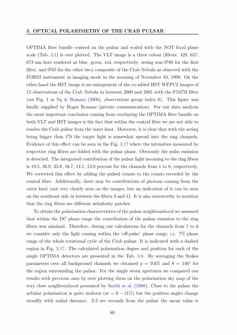
3. OPTICAL POLARIMETRY OF THE CRAB PULSAR
OPTIMA fibre bundle centred on the pulsar and scaled with the NOT focal plane
scale (Tab. 3.1) is over plotted. The VLT image is a three colour (filters: 429, 657,
673 nm here rendered as blue, green, red, respectively; seeing was 0.′′80 for the first
filter, and 0.′′65 for the other two) composite of the Crab Nebula as observed with the
FORS2 instrument in imaging mode in the morning of November 10, 1999. On the
other hand the HST image is an enlargement of the co-added HST WFPC2 images of
12 observations of the Crab Nebula in between 2000 and 2001 with the F547M filter
(see Fig. 1 in Ng & Romani (2006), observations group index 6). This figure was
kindly supplied by Roger Romani (private communication). For our data analysis
the most important conclusion coming from overlaying the OPTIMA fibre bundle on
both VLT and HST images is the fact that within the central fibre we are not able to
resolve the Crab pulsar from the inner knot. Moreover, it is clear that with the seeing
being bigger than 1.′′0 the target light is somewhat spread into the ring channels.
Evidence of this effect can be seen in the Fig. 3.17 where the intensities measured by
respective ring fibres are folded with the pulsar phase. Obviously the pulse emission
is detected. The integrated contribution of the pulsar light incoming to the ring fibres
is 19.5, 30.9, 33.8, 16.7, 14.1, 13.0 percent for the channels from 1 to 6, respectively.
We corrected this effect by adding the pulsed counts to the counts recorded by the
central fibre. Additionally, there may be contributions of photons coming from the
outer knot (not very clearly seen on the images, but an indication of it can be seen
on the southeast side in between the fibres 3 and 4). It is also noteworthy to mention
that the ring fibres see different nebulosity patches.
To obtain the polarisation characteristics of the pulsar neighbourhood we assumed
that within the DC phase range the contribution of the pulsar emission to the ring
fibres was minimal. Therefore, during our calculations for the channels from 1 to 6
we consider only the light coming within the ‘off-pulse’ phase range, i.e. 7% phase
range of the whole rotational cycle of the Crab pulsar. It is indicated with a dashed
region in Fig. 3.17. The calculated polarisation degree and position for each of the
single OPTIMA detectors are presented in the Tab. 3.8. By averaging the Stokes
parameters over all background channels we obtained p = 9.6% and θ = 140 for
the region surrounding the pulsar. For the single seven apertures we compared our
results with previous ones by over plotting them on the polarisation sky map of the
very close neighbourhood presented by Smith et al. (1988). Close to the pulsar the
nebular polarisation is quite uniform (at ∼ 9 − 11%) but the position angles change
steadily with radial distance. 2-3 arc seconds from the pulsar the mean value is
80

3.4 Results
0.0 0.2 0.4 0.6 0.8 1.0Phase
1500
2000
2500
3000
Inte
nsity
[Cou
nts]
Ch 1
Ch 2
Ch 3
Ch 4
Ch 5
Ch 6
0 60 120 180Polarization Filter Angle [degree]
200
250
300
350
400
450
Cou
nts
Ch 0
Ch 1
Ch 2
Ch 3
Ch 4
Ch 5
Ch 6
Figure 3.17: Upper : Light curves obtained from photons recorded by the ring fibresAPDs. All events were folded with the rotational parameters of the Crab pulsar.Dashed region between 0.78–0.84 phases indicates phase range of data that were latertaken to calculate θ and p for the ring fibres. Bottom: The sinusoidal modulation ofthe incoming polarised light, summed over the pulsar phase. Its amplitude varies fordifferent channels, because each channel is observing a bit different sky region.
81

3. OPTICAL POLARIMETRY OF THE CRAB PULSAR
Table 3.8: Left: p and θ results of the OPTIMA at NOT measurements of theCrab Nebula measured at the DC phase range of the Crab pulsar light curve (0.78–0.84, for details see upper panels of Fig. 3.17 and 3.18). Right: polarisation of theCrab Nebula as measured at minimum phase of the pulsar light curve. The axes arecalibrated in arcseconds centred on the pulsar, source Smith et al. (1988). ScaledOPTIMA fibre bundle is over plotted. The aperture of a single fibre is 2.′′35. Pinkline for central fibre and red lines for ring fibres represent our measurements.
Channel p [%] θ []0 33.20 118.91 8.95 141.62 10.22 142.63 8.69 148.34 9.21 136.55 11.42 133.16 10.18 138.0
1÷6 9.62 139.8
around 140 but beyond 5 arc seconds the position angle exceed 155 and it is very
direction-dependent (McLean et al. 1983).
3.4.2 Time alignment between optical and radio wavelengths
Precise timing of pulsar light curves throughout the electromagnetic spectrum can be
used to constrain theories of the spatial distribution of various emission regions and
their specific propagation delays. In the radio regime this concept has been applied in
the so called frequency mapping analysis. By dint of recent observations at different
energies, it became clear that the Crab pulsar emission maxima of IP and MP are not
aligned in phase at different wavelengths of the electromagnetic spectrum, from radio
to γ energy range. Comparing the visible and UV light curves obtained from HST,
Percival et al. (1993) were among the first to show that the phase separation between
the two peaks, ipso facto the phases of the pulse maxima, change with energy. Since
then many authors have measured this effect in an attempt to understand its relation
to and impact on the emission mechanism. However, the techniques used by different
authors to measure the phase separation (i.e. the phases of the peak maxima) have
varied. Therefore, this might cause method-dependent biases. Eikenberry & Fazio
82

3.4 Results
(1997) showed that the peak-to-peak separation appears to be a more or less smooth
function of energy from infrared to γ-ray energies. The separation decreases with
energy over the range from 0.5 to 106 eV from 0.4087 ± 0.0003 to 0.398 ± 0.003,
respectively. There is some evidence of a turnover or a break in this trend at energies
of 0.7 eV (H band pass filter). No default method exists for determining the position
of the peak of the profile. For our purpose and using our high statistics light curve it
was enough to determine the peak phases just by looking for the maximum intensity.
This gave us the phase values for the MP: 0.993 ± 0.001 and the IP: 0.398 ± 0.001
(Tab. 3.9). Our peak-to-peak separation is on the level of 0.4050 ± 0.0014. It is in
very good agreement with the values obtained by Eikenberry & Fazio (1997) for the
visual pass band, i.e. 0.4057 ± 0.0003, and from a previous OPTIMA observation
Straubmeier (2001) of 0.4060 ± 0.0003.
Optical, X-ray and γ-ray maxima of the MP are leading the radio pulse. At the
X- and γ−rays energies the picture is very much consistent, whereas at the optical
wavelength results obtained by different authors varies significantly. The reported
values of the time lags between TOA of optical and radio maxima are as follow:
344±40 µs (Rots et al. 2004, RXTE data), 280±40 µs (Kuiper et al. 2003, INTEGRAL
data), and 241 ± 29 µs (Kuiper et al. 2003, EGRET data). The uncertainty of the
latter value does not include the EGRET absolute timing uncertainty of better than
100 µs . At optical wavelengths the situation is quite different and does not provide
such a coherent picture. Several authors reported the optical peak leading the radio
peak by a time shift of 140 ± 78 µs (Sanwal 1999), 100 ± 20 µs (Shearer et al. 2003),
and 273±100 µs lately found by Oosterbroek et al. (2006). On the other hand Golden
et al. (2000b) reported that the optical pulse trails the radio pulse by about 80±60 µs.
Additionally, Romani et al. (2001) concluded that both, radio and optical, peaks are
coincident to better than 30 µs, but they did not take into account the uncertainty
of the radio ephemeris being on the level of 150 µs in their error calculations. From
our measurements we conclude that the optical is leading the radio by a time shift of
231±68 µs. The uncertainty in this value is 33 µs in the determination of the optical
peak of the MP and 60 µs in the radio ephemeris.
Our value of the optical phase difference between the MP and the IP of 0.4050 ±0.0014 is consistent with the latest optical measurements carried out by Oosterbroek
et al. (2006), who obtained 0.4054 ± 0.0004. Both values, as it has already been
shown by Eikenberry & Fazio (1997), are not consistent with the X-ray results, e.g.
obtained from RXTE data by Rots et al. (2004) of 0.4001±0.0002. This implies that
the details of the pulse profile in X-rays and in optical domain are different. In a simple
83

3. OPTICAL POLARIMETRY OF THE CRAB PULSAR
geometrical model (ignoring relativistic effects) a time shift of ∼ 231 µs indicates that
possibly the optical radiation is formed ∼ 70 km higher in the magnetosphere than
the radio emission. The difference in phase of 0.007 could also be interpreted as an
angle between the radio and optical beam of ∼ 2.5.
3.4.3 Polarisation characteristics of the Crab pulsar
The Crab pulsar is detected at all phases of rotation (Fig. 3.18), i.e. also in the
so-called ‘off-pulse’ phase with an intensity of about 2% compared to the intensity
of the MP maximum. In the literature one can find that the measured level of the
DC differs from author to author. For example very early measurements performed
by Peterson et al. (1978) gave the ‘unpulsed background’ from the Crab pulsar on
the level of 3.6% of the main peak intensity. Much lower values were obtained by
Jones et al. (1981) and later by Smith et al. (1988): 0.6% and 1.2%, respectively. In
addition Percival et al. (1993) claims that the ‘off-pulsed’ flux has an intensity less
than 0.9% of the peak flux (visible and UV data from HST , 2σ upper limit), whereas
a fractional flux derived by Golden et al. (2000a) from photometric analysis gives
∼ 1%.
For the background (nebula and sky) subtraction we took the averaged Stokes pa-
rameters recorded in the ring fibres over the ‘off-pulse’ phase. After subtracting this
steady component from the raw central channel a measurement of the three Stokes
parameters as a function of the rotational pulsar phase was derived (see Fig. 3.15).
The first Stokes parameter is of course intensity I. Pulse phase colour coded I, mea-
sured in counts, is shown in the upper panel of Fig. 3.18. The same, but normalised,
is shown on the logarithmic scale in the bottom panel. The colour coded Stokes pa-
rameters Q, U as a vector diagram are shown in Fig. 3.19. Colours refer to the pulse
phases as indicated in Fig. 3.18 and the scale is such that I = 100 at the maximum
light, i.e maximum of the MP. The MP and IP maxima are indicated with diamonds.
Points belonging to the MP phases follow an outer ellipse (upper panel), whereas
these belonging to the IP an inner one (bottom panel). In both cases the direction is
counter-clockwise. Noteworthy is that already from the Stokes parameters it is easy
to see that there is sudden change in the pattern near the radio phase, i.e. where
the red triangles change to the black ones. As the next step of the data analysis the
polarisation characteristics - the position angle and the degree of polarisation of the
E-vector - were calculated from the Stokes parameters. The results, plotted with a
resolution of 1000 phase bins, are presented in Fig. 3.20 and 3.21, respectively.
84
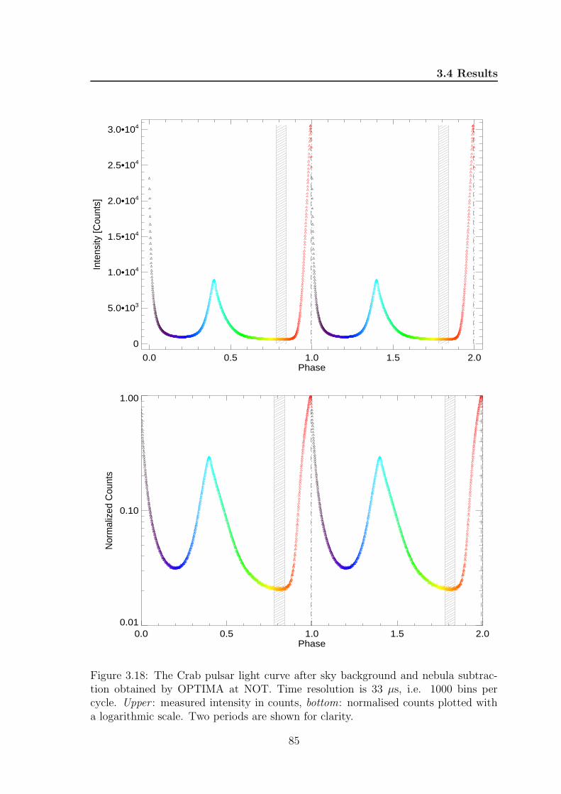
3.4 Results
0.0 0.5 1.0 1.5 2.0Phase
0
5.0•103
1.0•104
1.5•104
2.0•104
2.5•104
3.0•104
Inte
nsity
[Cou
nts]
0.0 0.5 1.0 1.5 2.0Phase
0.01
0.10
1.00
Nor
mal
ized
Cou
nts
Figure 3.18: The Crab pulsar light curve after sky background and nebula subtrac-tion obtained by OPTIMA at NOT. Time resolution is 33 µs, i.e. 1000 bins percycle. Upper : measured intensity in counts, bottom: normalised counts plotted witha logarithmic scale. Two periods are shown for clarity.
85

3. OPTICAL POLARIMETRY OF THE CRAB PULSAR
-8 -6 -4 -2 0Q
-6
-4
-2
0
U
MP max
IP max
-3 -2 -1 0 1Q
-3
-2
-1
0
1
U
IP max
Figure 3.19: Stokes parameters Q, U as a vector diagram. Colours refer to the pulsephases as indicated in Fig. 3.18. The scale is such that I = 100 at the maximum light.Phases of the MP and IP maxima are indicated with diamonds. Triangles belongingto the MP and IP follow in a counter-clockwise direction an outer and inner ellipse,respectively. Bottom panel shows a zoomed region around the IP phases as it isindicated with a black frame in the upper panel. Dashed lines are the horizontal andvertical line at the zero level.
86
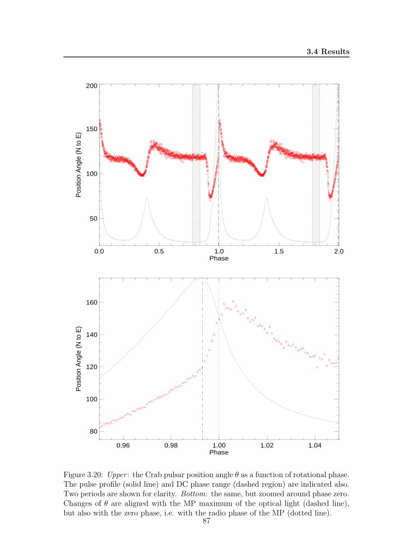
3.4 Results
0.0 0.5 1.0 1.5 2.0Phase
50
100
150
200P
ositi
on A
ngle
(N to
E)
0.96 0.98 1.00 1.02 1.04Phase
80
100
120
140
160
Pos
ition
Ang
le (N
to E
)
Figure 3.20: Upper : the Crab pulsar position angle θ as a function of rotational phase.The pulse profile (solid line) and DC phase range (dashed region) are indicated also.Two periods are shown for clarity. Bottom: the same, but zoomed around phase zero.Changes of θ are aligned with the MP maximum of the optical light (dashed line),but also with the zero phase, i.e. with the radio phase of the MP (dotted line).
87

3. OPTICAL POLARIMETRY OF THE CRAB PULSAR
0.0 0.5 1.0 1.5 2.0Phase
0
10
20
30
40
50
Pol
ariz
atio
n de
gree
[%]
0.96 0.98 1.00 1.02 1.04Phase
0
5
10
15
20
Pol
ariz
atio
n de
gree
[%]
Figure 3.21: Upper : the Crab pulsar polarisation degree p as a function of rotationalphase. The pulse profile (solid line) and DC phase range (dashed region) are indicatedalso. Two periods are shown for clarity. Bottom: the same, but zoomed around thephase zero. Minimum of p is for the radio phase (dotted line), and not for themaximum phase of the optical MP (dashed line).
88

3.5 Summary and discussion
3.4.4 Polarisation characteristics of the Crab pulsar after DCsubtraction
The apparent constancy of the position angle within the phase range 0.78–0.84 (Fig.
3.20, upper panel) may suggest that the optical emission from the Crab pulsar consists
of two components - pulsed and unpulsed. The pulsed component is characterised
by a highly variable position angle and polarisation degree. The unpulsed (i.e. DC)
component is characterised by constant intensity on the level of 2% of the main pulse
intensity, fixed θ ∼ 119, and a degree of polarisation on the level of 33%. The
source of emission of the DC is unknown. There are various ideas from where in the
magnetosphere or the nebula this component might arise. It is also possible that the
inner knot (located only 0.′′65 apart from the pulsar and being a persistent feature
throughout the sequences of HST images, Hester et al. (2002)) is responsible for the
‘off-pulse’ emission. Assuming that the unpulsed component is present at all phase
angles and has constant polarisation we obtained the polarisation characteristics of
the ‘pulsed component’ separately by subtracting the respective Stokes parameters
I, Q, U from the linear polarisation data. The results are presented in Fig. 3.22,
3.23, and 3.24. After subtracting the ‘unpulsed component’ the position angle and
polarisation degree in the phases where the intensity is very low are not well defined.
Because the Stokes parameters go basically to zero for these rotational phases, the
values of θ and p become very noisy.
The polarisation degree of the ‘off-pulse’ component obtained in this work differs
from the values presented by other authors (e.g. Jones et al. (1981): ∼ 70%; Smith
et al. (1988): ∼ 47%± 10%). This might be caused by two reasons. Firstly, different
groups treat background subtraction in different ways. Additionally, all mentioned
observations were taken during different epochs and with different instrumentation.
Secondly, the observed variation might be caused by the intrinsic mechanism of the
pulsar and/or nebula radiation. We note also that one would expect a change in flux
of ∼ 0.066 over the 22 years between Jones et al. (1981) and our observations, follow-
ing the phenomenologically derived LV ∼ 0.003 mag yr−1 (Pacini 1971), empirically
confirmed most recently by Nasuti et al. (1997).
3.5 Summary and discussion
The Crab pulsar emits highly anisotropic radiation which spans a wide range of wave-
lengths, from radio to extreme γ-rays. Knowledge of polarisation characteristics of
this radiation is of fundamental importance in our attempts to find the mechanisms
89

3. OPTICAL POLARIMETRY OF THE CRAB PULSAR
-8 -6 -4 -2 0 2Q
-4
-2
0
2
U
MP max
IP max
-3 -2 -1 0 1Q
-3
-2
-1
0
1
U
IP max
Figure 3.22: The same as in Fig. 3.19 but after DC subtraction.
90

3.5 Summary and discussion
0.0 0.5 1.0 1.5 2.0Phase
50
100
150
200P
ositi
on A
ngle
(N
to E
)
0.96 0.98 1.00 1.02 1.04Phase
80
100
120
140
160
Pos
ition
Ang
le (
N to
E)
Figure 3.23: The same as in Fig. 3.20 but after DC subtraction.
91

3. OPTICAL POLARIMETRY OF THE CRAB PULSAR
0.0 0.5 1.0 1.5 2.0Phase
0
10
20
30
40
50
Pol
ariz
atio
n de
gree
[%]
0.96 0.98 1.00 1.02 1.04Phase
0
5
10
15
20
Pol
ariz
atio
n de
gree
[%]
Figure 3.24: The same as in Fig. 3.21 but after DC subtraction.
92

3.5 Summary and discussion
Table 3.9: p and θ for three selected Crab pulsar phases, i.e. the radio phase, and thephases of both optical maxima, MP and IP. Values before and after DC componentsubtraction are shown.
After DC SubtractionPhase p [%] θ [] p [%] θ []
Radio 0.000 3.29 149.60 3.04 157.46max of MP 0.993 5.92 119.75 5.34 119.87max of IP 0.398 7.61 109.87 5.83 105.98
responsible for Crab’s magnetospheric activity. Good quality X-ray and gamma-ray
polarimetry with satellite observatories is expected to be available for pulsar studies
(among other types of objects) in the near future. Present-day state of instrumenta-
tion is sufficient to carry out optical polarimetry of this object with unprecedented
quality. Our project to study the Crab Pulsar with OPTIMA and NOT is, to the best
of our knowledge, the most recent and most complete one. The observations with
33 µs time resolution are a factor of 4 better than the previous best observations. We
have completely resolved the polarisation characteristics of both peaks of the Crab
pulsar, MP and IP, in the optical pass bands (see Fig. 3.25). Moreover, we were able
to better characterise the polarised emission between the peaks, i.e. in the so called
‘bridge’ as well as the DC (often referred as the ‘off-pulse’ component) regions. We
find that the MP of the Crab pulsar arrives 231 ± 68 µs before the peak of the radio
pulse.
The phase averaged polarisation degree of the Crab pulsar amounts to 9.82% with
a position angle of 109.5. After the DC subtraction it is 5.48% and 96.3, respectively.
Minimum polarisation degree occurs at the phase of 0.999 (see Tab. 3.9), very close
to the radio pulsar phase, with p = 3.3%, θ = 149.6 before the DC subtraction, and
with p = 3.0%, θ = 157.5 after DC subtraction. During the IP the minimum value
of p is on the level of 5%, before DC subtraction. Similar to the MP case, it is also
shifted (with respect to the phase of the optical maximum) to the leading wing of the
pulse. The value of p changes after DC subtraction to ∼ 2%. This means that the
situation is inverted: before the DC subtraction the minimum of p is reached during
the main pulse, whereas after this subtraction the minimum polarisation degree is
observed during the inter pulse.
Our results agree generally well with previous measurements (e.g. Kanbach et al.
2005; Smith et al. 1988), but they show details with much better definition and
statistics (see Fig. 3.26 for comparison). The behaviour of θ as a function of phase
observed for the Crab pulsar at optical wavelengths (Fig. 3.20) differ from those
93
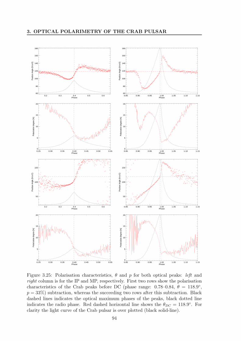
3. OPTICAL POLARIMETRY OF THE CRAB PULSAR
0.2 0.3 0.4 0.5 0.6Phase
60
80
100
120
140
160
180
Pos
ition
Ang
le (N
to E
)
0.85 0.90 0.95 1.00 1.05 1.10 1.15Phase
60
80
100
120
140
160
180
Pos
ition
Ang
le (N
to E
)
0.25 0.30 0.35 0.40 0.45 0.50 0.55Phase
0
5
10
15
20
Pol
ariz
atio
n de
gree
[%]
0.85 0.90 0.95 1.00 1.05 1.10 1.15Phase
0
5
10
15
20
Pol
ariz
atio
n de
gree
[%]
0.2 0.3 0.4 0.5 0.6Phase
50
100
150
Pos
ition
Ang
le (N
to E
)
0.85 0.90 0.95 1.00 1.05 1.10 1.15Phase
50
100
150
Pos
ition
Ang
le (N
to E
)
0.25 0.30 0.35 0.40 0.45 0.50 0.55Phase
0
5
10
15
20
Pol
ariz
atio
n de
gree
[%]
0.85 0.90 0.95 1.00 1.05 1.10 1.15Phase
0
5
10
15
20
Pol
ariz
atio
n de
gree
[%]
Figure 3.25: Polarisation characteristics, θ and p for both optical peaks: left andright column is for the IP and MP, respectively. First two rows show the polarisationcharacteristics of the Crab peaks before DC (phase range: 0.78–0.84, θ = 118.9,p = 33%) subtraction, whereas the succeeding two rows after this subtraction. Blackdashed lines indicates the optical maximum phases of the peaks, black dotted lineindicates the radio phase. Red dashed horizontal line shows the θDC = 118.9. Forclarity the light curve of the Crab pulsar is over plotted (black solid-line).
94

3.5 Summary and discussion
0.0 0.5 1.0 1.5 2.0Phase
0
20
40
60
80
100
Inte
nsity
[Cou
nts]
0.0 0.5 1.0 1.5 2.0Phase
60
80
100
120
140
160
Pos
ition
Ang
le (N
to E
)
0.0 0.5 1.0 1.5 2.0Phase
0
20
40
60
80
100
Pol
ariz
atio
n de
gree
[%]
-8 -6 -4 -2 0Q
-6
-4
-2
0
U
MP max
IP max
Figure 3.26: Comparison of the results obtained by Smith et al. (1988) and this workright and left column, respectively. From top to bottom: the intensity, position angle,polarisation degree, and the Stokes parameters Q, U plotted as a vector diagram asa function of the pulsar phase. There are 250 bins per cycle in both cases, the onlydifference is that for clarity we show two periods. As a DC component Smith et al.took 50 out of 250 bins, whereas we took only 7% of the rotational period.
95

3. OPTICAL POLARIMETRY OF THE CRAB PULSAR
observed at radio wavelengths (e.g. Karastergiou et al. 2004; Moffett & Hankins 1999;
S lowikowska et al. 2005a). Two factors may be responsible for this difference: different
propagation effects, and different intrinsic emission mechanisms. In particular, the
former factor plays an essential role in such high-energy emission models like the
outer gap model or the two-pole caustic model: in both models high-energy emission
comes from a very wide range of altitudes, contrary to radio emission which originates
within a narrow range of altitudes. For comparison the light curves and polarisation
characteristics obtained within the framework of three high energy magnetospheric
emission models of pulsars, i.e. the polar cap model, the two-pole caustic model, and
the outer gap model are shown in Fig. 3.27.
Crab Pulsar
0
1
2
3
Inte
nsity
50
100
150
200
Pos
ition
ang
le
-0.4 -0.2 0.0 0.2 0.4 0.6 0.8phase
0.0
0.1
0.2
0.3
0.4
0.5
Deg
ree
of p
olar
izat
ion
Polar cap modelα=7°, ζ=12°
-0.4 -0.2 0.0 0.2 0.4phase
0
1
2
3
Two-pole caustic modelα=70°, ζ=50°
-50
0
50
-0.2 0.0 0.2 0.4 0.6phase
0.0
0.2
0.4
0.6
0.8
1.0
Outer gap modelα=65°, ζ=82°
0.0 0.2 0.4 0.6 0.8phase
Figure 3.27: The optical light curve, the position angle θ and the degree of polarisationp calculated with the following models of high energy radiation from pulsars, from leftto right : the polar cap model, the two-pole caustic model, and the outer gap model(Dyks et al. 2004b). In the first column, the data from Calar Alto observations(Kanbach et al. 2005) are shown for comparison. Courtesy J. Dyks.
The two-pole caustic model (Dyks & Rudak 2003) predicts fast swings of the po-
sition angle and minima in the polarisation degree, similar to what is observed. Polar
cap model and outer gap model are not able to reproduce the observational polar-
isation characteristics of the Crab pulsar. Another model, placing the origin of the
pulsed optical emission from the Crab in a striped pulsar wind zone has recently been
96

3.6 Conclusions
proposed by Petri & Kirk (2005). This model features also polarisation characteristics
that bear a certain resemblance to the observations.
3.6 Conclusions
The optical emission from the Crab pulsar is highly polarised, especially in the bridge
and ‘off-pulse’ phases. The position angle θ and polarisation degree p of linear polar-
isation as a function of rotation phase show well determined properties:
a) the polarisation characteristics of the two pulse components, MP and IP, are
very similar;
b) the polarisation degree is minimal at the phases of the maximum radio intensity,
therefore, it is NOT aligned with the optical peaks;
c) there is a well defined bump in polarisation degree on the rising flank of MP,
d) there is an indication of such a bump also for IP, especially after the DC sub-
traction;
e) the polarisation angle swings through a large angle in both peaks: after subtrac-
tion of an assumed constant polarisation component (intensity on the level of
2% of the MP) the angle swing is 130 and 100 for the MP and IP, respectively.
Theoretical models, like the two-pole caustic model (Dyks, Harding, & Rudak 2004a)
or the striped pulsar wind model (Petri & Kirk 2005) are able to reproduce (at least
qualitatively) some of these properties, e.g. (a) and (e). However, full explanation of
the properties (a) to (e) will require more detailed models to be developed.
97

Chapter 4
PSR B0540-69 - the Crab twin inthe Large Magellanic Cloud
4.1 Introduction
PSR B0540-69, a 50 ms pulsar located in the Large Magellanic Cloud (LMC), is one
of the most distant pulsars known (d = 49.4 ± 3.36 kpc, Taylor & Cordes 1993).
Seward et al. (1984) discovered the pulsar at the position of supernova remnant
SNR 0540-693 by using the Einstein X-Ray Observatory. Shortly after its discovery
a bright synchrotron wind nebula was confirmed in the optical waveband (Chanan
et al. 1984). The optical pulsations were soon detected by Middleditch & Pennypacker
(1985) with a mean pulsed magnitude of 22.5. In the radio band the pulsar is quite a
faint source (Manchester et al. 1993), though Johnston & Romani recently reported
the discovery of the first giant pulses from this pulsar (Johnston & Romani 2003).
Since 1984 PSR B0540-69 has been observed by: HST (Boyd et al. 1995; Serafimovich
et al. 2004),VLT (Serafimovich et al. 2004), BeppoSAX (Mineo et al. 1999), GINGA
(Deeter et al. 1999), Chandra X-ray Observatory (Gotthelf & Wang 2000; Kaaret
et al. 2001), ASCA (Hirayama et al. 2002) and RXTE (de Plaa et al. 2003).
PSR B0540-69 is often referred to as an extragalactic ‘twin’ of the Crab pulsar
(Tab. 4.1). Both pulsars have similar rotational parameters, characteristic age, spin-
down luminosity and both are embedded in synchrotron plerionic nebulae (Figs. 4.1
and 1.7). Here the similarity ends. Pulse profiles and spectra of PSR B0540-69 and
PSR B0531+21 differ significantly. The Crab pulse profile shows a sharp double-peak
structure, whereas the profile of LMC pulsar consists of a single broad peak. However,
this broad pulse peak might be formed as a superposition of two Gaussian components
separated of about 0.2 in phase (de Plaa et al. 2003). The X-ray spectrum of PSR
98

4.2 The INTEGRAL satellite
Table 4.1: Properties of PSR B0540-69 and the Crab pulsar.
Parameter PSR B0540-69 PSR B0531+21P (s) 0.05035 0.03308
P (s s−1) 4.79 × 10⁻¹³ 4.23 × 10⁻¹³
n 2.08 2.51d (kpc) 49.40 2.0τc (kyr) 1.67 1.24Bs (G) 4.97 × 10¹² 3.78 × 10¹²
Lsd (erg s−1) 1.5 × 1038 4.6 × 1038
Nebula size (pc) 0.6 × 0.9 1.5 × 1.5
B0540-60 (de Plaa et al. 2003) differs from thet Crab spectrum. Additionally, unlike
the Crab pulsar, PSR B0540-69 is not a γ-ray pulsar.
Figure 4.1: Left : The X-ray and radio maps of the region of SNR 0540-693. PSRB0540-69 is located in the centre. Contours reflect the Chandra HRC X-ray inten-sity distribution, whereas the green-scale map denotes the radio emission at 6 cm(Manchester et al. 1993). Middle: The X-ray Chandra HRC image centred on thepulsar. Region indicated by the central box is enlarged and displayed in the nextpanel. Right : Close-up image around the pulsar. There is a marginal evidence fora jet-like feature emanating from the pulsar. Inset : The Crab Nebula image, placedat the distance of the LMC. The image was blurred to the Chandra HRC resolution.Both nebulae are similar in size. Moreover, they have broadly similar shape andoverall brightness morphology [Gotthelf & Wang (2000)].
4.2 The INTEGRAL satellite
The International Gamma-Ray Astrophysics Laboratory (INTEGRAL) is a 15 keV
– 10 MeV gamma-ray observatory mission, consisting of the spectrometer SPI and
the imager IBIS (Sec. 4.4), with concurrent source monitoring in X-rays - the Joint
99

4. PSR B0540-69 - THE CRAB TWIN IN THE LARGE MAGELLANICCLOUD
European Monitor for X-rays (JEM-X, 3–35 keV, Sec. 4.5) and in the optical range -
the Optical Monitoring Camera (OMC, V, 500–600 nm).
High resolution spectroscopy over the entire energy range permits spectral features
to be uniquely identified and line profiles to be determined for physical studies of the
source and its surrounding. The fine imaging capability of INTEGRAL within a
large field of view allows an accurate source localisation. The identification of the
gamma-ray emitting objects with their counterparts at other wavelengths enables to
distinguish extended regions from point sources. Characteristic parameters of two
main INTEGRAL instruments; spectrometer SPI and imager IBIS are presented in
Tab. 4.2
Table 4.2: Characteristics of the two main INTEGRAL instruments, the spectrometerSPI and the imager IBIS
SPI IBIS
Energy range 20 keV – 8 MeV 15 keV – 10 MeVDetectors 19 Ge 16384 CdTe (ISGRI)
cooled to 85 K 4096 CsI (PICsIT)Detector area (cm2) 500 2600 (CdTe), 3100 (CsI)Spectral resolution (FWHM) 2.3 keV @ 1.3 MeV 9 keV @ 100 keVField of view (fully coded) 16(corner to corner) 9 × 9
Angular resolution (FWHM) 2.5(point source) 12′
Source location (radius) < 1.3 (depenging on < 1′ (for 10σ source)the source strength)
Absolute timing accuracy (3σ) 129 µs 61 µs
4.3 Observations
We gathered more than one million seconds of PSR B0540-69 observations with IN-
TEGRAL. One INTEGRAL orbit that lasts three sidereal days makes one revolution.
The satellite was pointed to the LMC during nine revolutions (Tab. 4.3); six of them
took place in January 2003 and three of them a year later, in January 2004. Because
of the dithering of the INTEGRAL satellite, single observation consists of many point-
ings that last about 30 minutes and are separated by slews. Each pointing and slew,
or only a part of them if they are too long, is called a Science Window (ScW). Single
observation usually consists of several ScWs. Detailed information about the strat-
egy of scientific observations, as well as about the hierarchical data storage and data
repositories can be found in the ”Introduction to the INTEGRAL data analysis”1.
1http://isdc.unige.ch/index.cgi?Soft+download
100

4.3 Observations
Table 4.3: Time span of the INTEGRAL LMC observations. A total of 813 ScWswithin nine revolution were selected. First column gives the INTEGRAL orbit (revo-lution) number. Second column shows the arbitrary numbers of ScWs given in brack-ets, as well as a total number of ScWs in revolution. Next columns show revolutionstart and end time given in MJD TT and UTC, respectively.Rev Number of ScWs TSTART TSTOP TSTART TSTOP0027 (1-92) 92 52641.33 52643.98 2003Jan02 at 07:57:54 2003Jan04 at 23:38:550028 (93-177) 85 52644.33 52646.97 2003Jan05 at 08:01:21 2003Jan07 at 23:29:570029 (178-271) 94 52647.33 52649.97 2003Jan08 at 07:55:09 2003Jan10 at 23:20:020033 (272-367) 96 52659.29 52661.94 2003Jan20 at 06:58:11 2003Jan22 at 22:34:560034 (368-459) 92 52662.29 52664.93 2003Jan23 at 07:09:39 2003Jan25 at 22:19:590035 (460-552) 93 52665.27 52667.94 2003Jan26 at 06:29:29 2003Jan28 at 22:34:580150 (553-631) 79 53009.26 53011.93 2004Jan05 at 06:14:46 2004Jan07 at 22:29:590151 (632-726) 95 53012.23 53014.92 2004Jan08 at 05:37:33 2004Jan10 at 22:14:570152 (727-813) 87 53015.22 53017.93 2004Jan11 at 05:25:23 2004Jan13 at 22:21:52
Additional information is provided in the manuals published by INTEGRAL Science
Data Centre (ISDC) team. For the purpose of our project we used public INTEGRAL
software - Off-line Science Analysis (OSA, v5.1). It is supported by ISDC. For the
timing analysis we used our own IDL procedures.
Detailed description of the data selection
We used all available INTEGRAL data of PSR B0540-69. Until now the LMC was ob-
served during the following nine revolutions: 0027, 0028, 0029, 0033, 0034, 0035, 0150,
0151 and 0152 (Tab. 4.3). It resulted in 813 ScWs operated in the pointing mode.
The exposure time in seconds, as well as the position angle in degrees as a function
of selected ScWs is shown in the Fig. 4.2. Arbitrary ScW numbers corresponding
to different revolutions are given in Tab. 4.3. Afterwards, we made the following
selection. Using idx find1 we requested for: ScW being of pointing type, pulsar lo-
cated in the fully illuminated field of view (that is 9 and 4.8 for IBIS and JEM-X,
respectively), and both instrument modes being equal to 41, i.e. IBISMODE=41 and
JMX2MODE=41. We obtained two lists of ScWs fulfilling the terms of our criteria.
The IBIS list consists of 617 ScWs, and the JEM-X one of 409 ScWs. None the less,
in both cases the final number of used ScWs decreased during the analysis. It was
caused by different reasons that are discussed in the according paragraphs.
Both, IBIS and JEM-X are coded mask instruments, therefore it is not possible
to deal with one source at a time. Each source contributes to the background of
the other sources detected in the field of view (FoV) of the instrument. Thus, all
1This procedure allows to select ScWs fulfilling terms of user criteria.
101
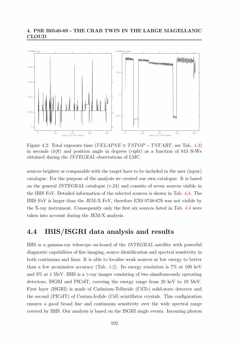
4. PSR B0540-69 - THE CRAB TWIN IN THE LARGE MAGELLANICCLOUD
0 200 400 600 800
0
2000
4000
6000
8000
Arbitrary ScW Number
TELAPSE (s)
0 200 400 600 800
-100
0
100
Arbitrary ScW Number
POSANGLE (deg)
Figure 4.2: Total exposure time (TELAPSE ≡ TSTOP − TSTART , see Tab. 4.3)in seconds (left) and position angle in degrees (right) as a function of 813 ScWsobtained during the INTEGRAL observations of LMC.
sources brighter or comparable with the target have to be included in the user (input)
catalogue. For the purpose of the analysis we created our own catalogue. It is based
on the general INTEGRAL catalogue (v.24) and consists of seven sources visible in
the IBIS FoV. Detailed information of the selected sources is shown in Tab. 4.4. The
IBIS FoV is larger than the JEM-X FoV, therefore EX0 0748-676 was not visible by
the X-ray instrument. Consequently only the first six sources listed in Tab. 4.4 were
taken into account during the JEM-X analysis.
4.4 IBIS/ISGRI data analysis and results
IBIS is a gamma-ray telescope on-board of the INTEGRAL satellite with powerful
diagnostic capabilities of fine imaging, source identification and spectral sensitivity in
both continuum and lines. It is able to localise weak sources at low energy to better
than a few arcminutes accuracy (Tab. 4.2). Its energy resolution is 7% at 100 keV
and 9% at 1 MeV. IBIS is a γ-ray imager consisting of two simultaneously operating
detectors, ISGRI and PICsIT, covering the energy range from 20 keV to 10 MeV.
First layer (ISGRI) is made of Cadmium-Telluride (CdTe) solid-state detector and
the second (PICsIT) of Cesium-Iodide (CsI) scintillator crystals. This configuration
ensures a good broad line and continuum sensitivity over the wide spectral range
covered by IBIS. Our analysis is based on the ISGRI single events. Incoming photon
102

4.4 IBIS/ISGRI data analysis and results
Table 4.4: Catalogue of selected sources used for the IBIS/ISGRI and JEM-X analysis.Coordinates are given in the increasing order of RA. Additionally the ISGRI (I FLAG)and JEM-X (J FLAG) detection flags are given; 0 - undetected, 1 - detected. However,the flag values are obtained for the standard settings of the data analysis performedby ISDC team. Especially the minimum detection sigma parameter could play a rolehere. The source coordinates were taken from the INTEGRAL General ReferenceCatalogue (v.24) containing all sources detected by INTEGRAL and being brighterthan 1 mCrab above 1 keV. Only the pulsar position was changed. We used thecoordinates given by Kaaret et al. (2001) on the basis of the Chandra observation.
NAME SOURCE ID α [] δ [] I FLAG J FLAGLMC X-2 J052029.2-715736 80.12167 -71.96000 0 1LMC X-4 J053249.2-662214 83.205 -66.37056 1 1SN 1987A J053530.0-691600 83.875 -69.26667 0 0LMC X-3 J053856.4-640501 84.735 -64.08361 0 1LMC X-1 J053938.7-694436 84.91125 -69.74333 1 1
PSR B0540-69 J054007.7-692005 85.04675 -69.33194 1 0EXO 0748-676 J074833.8-674509 117.1408 -67.7525 1 0
is stopped in a single pixel of the ISGRI layer, generating an electric pulse. The
pulse amplitude yields the energy of the incident photon. However, above 50 keV the
energy is a function of not just the pulse height but also the pulse rise time. In that
case both measured values are used to determine the energy of the photon.
We constructed pulsar ephemeris from the Rossi X-ray Timing Explorer Mission
Proportional Counter Array (RXTE PCA) observations. The RXTE data were taken
between December, 7 2002 and January, 30 2003, as well as between January, 3 and
February, 27 2004. The ephemeris obtained for both epochs are presented in Tab. 4.5,
respectively. Note that second frequency derivative for the time span 53007–53062
MJD (Rev. 150–152) is not significant. The RXTE PCA 2–10 keV pulse profile
constructed by using the data collected over December 2002 and January 2003 and
folded accordingly to the pulsar ephemeris is shown in Fig. 4.3, left panel. The pulse
profiles obtained from the data collected between January and February 2004 in three
energy bands: 2–10, 10–20, and 20–30 keV are shown in Fig. 4.3, right panel. It is
clear that the pulse duty cycle increases, while the pulsed fraction likely decreases
with energy. The exact number of the pulsed fraction defined as f = NP
NP +NDCcan not
be derived because of the unknown background level. The ephemeris for 2003 and
2004 observations are not absolute, and the alignment of the corresponding RXTE
pulse profiles is not absolute either. Absolute timing would require defining the anchor
point in the profile and referencing to this phase.
103

4. PSR B0540-69 - THE CRAB TWIN IN THE LARGE MAGELLANICCLOUD
Table 4.5: PSR B0540-69 ephemeris.
Parameter & Value Valueα2000 05h40m11.s221δ2000 −6919′54.′′98
Rev. 27, 28, 29, 33, 34 and 35Val. range (MJD) 52620–52670t0 (TDB MJD) 52625.000000000ν0 (Hz) 19.779298587915ν0 (10−10 Hz s−1) −1.87410ν0 (10−20 Hz s−2) 2.51
Rev. 150, 151, 152Val. range (MJD) 53007–53062t0 (TDB MJD) 53007.000000000ν0 (Hz) 19.773116586988(11189)ν0 (10−10 Hz s−1) −1.87256(11)ν0 (10−21 Hz s−2) 3.413(4.92)
Since October 18, 2004 all public INTEGRAL data are available in two formats:
revision 1 (Rev.1) and revision 2 (Rev.2). In Rev.2, the correction of all JD time
stamps for the offsets between the On Board Time (OBT) of each instrument is done.
In Rev.2 the data correction (COR) step, as well as the instrumental Good Time
Interval (GTI) and deadline handling (DEAD) steps are performed by ISDC team
by using OSA (v.4.2) at the science window level. During the COR step the data
are corrected for instrumental effects, such as energy and position corrections, while
the GTI step generates, selects and merges Good Time Intervals to produce a unique
GTI that is later used for selecting events. The net observing time is also computed
in this step. Dead and live times are computed during DEAD step of the analysis.
The dead time is the time during which the instrument was not capable to register,
for different reasons, the incoming photons within GTI. However, the data correction
implemented in OSA 5.1 is much better. Therefore, it is highly recommended by the
ISDC team to rerun these three steps (COR, GTI, DEAD) over the used data. We
performed these correction steps over all selected ScWs, although it is very time and
disc-space consuming.
It is known from the ISGRI limitations that a problem on-board IBIS causes,
under some circumstances, event times to be shifted by 2 seconds. The OSA software
corrects for it, but still the possible jumps might occur. Such behaviour can be verify
by checking the value under the FITS flag keyword TIMECORR. For accurate timing
104

4.4 IBIS/ISGRI data analysis and results
Figure 4.3: Left : RXTE PCA 2–10 keV pulse profile of PSR B0540-69 obtainedform the data collected between December, 7 2002 and January, 30 2003. Right :RXTE PCA normalised pulse profiles of PSR B0540-69 obtained form the datacollected between January, 3 and February, 27 2004. The red, green, and blue lightcurves corresponds to 2–10, 10–20, and 20–30 keV energy bands, respectively. Thepulse duty cycle changes significantly with energy. The background level is unknown,therefore the pulsed fraction can not be measured.
it is recommended to use only the data with no possible jump, i.e. TIMECORR=0.
Therefore, we used only ScWs with TIMECORR equal 0. The most update version
of the known limitations, including list of ScWs for which the two-second jumps have
been detected, can be found on the ISDC web pages 1.
A standard and stand-alone tool ii pif built is used to calculate the ISGRI Photo
Illumination Fraction (PIF) for a given source. Once the PIF map is made, it is
straightforward to filter event lists based on the PIF threshold. By applying the PIF
filter, one can reduce the background and optimise the signal to noise ratio. From
experience, we choose PIF> 0.5 as the event selection criterion. We run ii pif built pro-
cedure with pulsar position (α2000 = 85.046754167, δ2000 = −69.331938889, Kaaret
et al. (2001)) as an input parameter to compute the PIF for each event. By using
the evts extract script only single events (evttype=0, 7 < RISE TIME < 90) were
selected. Additionally, the noisy pixels (SELECT FLAG=0) were filtered out. The
procedure evts extract allows to barycentre the events, however at this point we did
not use it. Firstly, the instrument time corrections were applied, i.e. 111 ± 10µs and
185 ± 10µs for IBIS and JEM-X, respectively (Walter et al. 2003) and then derived
1 http://isdc.unige.ch/Soft/download/osa/osa sw/osa sw-5.1/osa issues.txt
105

4. PSR B0540-69 - THE CRAB TWIN IN THE LARGE MAGELLANICCLOUD
times of arrivals (TOAs) were barycentred. Afterwards, only events with the energy
≤ 300 keV were selected. For these events we stored their TOAs, PIF and energy
values. TOAs belonging to the first and second set of observations were then folded
according to the corresponding RXTE ephemeris (Tab. 4.5). Hence, we obtained two
sets of the pulsar light curves in five energy bands: 17–25, 25–40, 40-100, 100-200, and
200-300 keV. The ephemeris are not absolute, therefore to sum up the light curves
from both observations we used the cross-correlation method. As the template we
used light curve with the highest significance, i.e. the light curve obtained for JEM-X
data in the 6-10 keV energy band (see Sec. 4.5). In the light curves only the events
with PIF > 0.5 are included, i.e. with probability of illuminating the pixel by the
source being higher than 50%. The results are presented in Fig. 4.4.
By standard data processing (ibis science analysis) we produced the sky images for
each individual ScW. The source is very faint, therefore it was not detected on high
significance level in single ScWs. The OSA software allows to gather the single ScWs
belonging to different observations. Thus, we used all selected ScWs to produce the
mosaic maps. They correspond to the same five energy bands used for the light curve
extraction. In the mosaic maps the PSR B0540-69 was detected in four lower energy
bands with following significances: 13.8, 11.2, 7.6 and 6.2, respectively (Figs. 4.6,
4.7). There was no significant detection above 200 keV.
For the faint sources the recommended spectral extraction method is based on the
mosaic sky images. To derive the spectrum we used the count rate values obtained
from these images. We derive the spectrum of the total source exclusively from the
ISGRI data, treating the calibration of JEM-X as not applicable to such a weak
source. The photon spectrum can be fitted with a power law of index -2.22, which is
compatible with the result found by Gotz et al. (2006). The spectrum and the power
law fit are shown in Fig. 4.5.
106

4.4 IBIS/ISGRI data analysis and results
Figure 4.4: PSR B0540-69 light curves obtained from JEM-X (left column) and IBIS(middle and right columns) instruments. The energy bands are indicated in eachpanel, two cycles are shown for clarity. The PIF values in the description of PIFranges were multiply by 10.
107

4. PSR B0540-69 - THE CRAB TWIN IN THE LARGE MAGELLANICCLOUD
Figure 4.5: PSR B0540-69 spectrum in 17–300 keV energy range. Above 200 keVonly upper limit was derived. The dashed line indicates the power law fit.
108

4.4
IBIS
/IS
GR
Idata
analy
sisand
resu
lts
Figure 4.6: The IBIS/ISGRI significance mosaic images of the LMC region (left) and the close-up of the pulsar neighbourhood(right). Maps are for the 17–25 keV (top) and 25–40 keV (bottom) energy ranges. PSR B0540-69 was detected with followingsignificance 13.8σ and 11.2σ, respectively.
109

4.
PSR
B0540-6
9-T
HE
CR
AB
TW
ININ
TH
ELA
RG
EM
AG
ELLA
NIC
CLO
UD
Figure 4.7: The IBIS/ISGRI significance mosaic images of the LMC region (left) and the close-up of the pulsar neighbourhood(right). Maps are for the 40–100 (top) and 100–200 keV (bottom) energy ranges. PSR B0540-69 was detected with followingsignificance 7.6σ and 6.2σ, respectively.
110

4.5 JEM-X data analysis and results
4.5 JEM-X data analysis and results
Joint European Monitor for X-rays (JEM-X) operates simultaneously with the main
γ-ray INTEGRAL instruments. It is based on the same principles as IBIS and SPI
instruments: sky imaging accomplished by a coded aperture mask based on a Hexag-
onal Uniformly Redundant Array (HURA). Its energy range is 3–35 keV, angular
resolution at FWHM is 3′, fully illuminated field of view is 4.8, while time resolution
is on the level of 122 µs and 1 ms for relative and absolute timing, respectively. We
used the data of the full imaging telemetry format only, i.e. the image resolution of
the detector was 256x256 pixels, timing resolution 1/8192 s = 122 µs, and spectral
resolution 256 Pulse Height Amplitude (PHA) channels. The position determination
accuracy depends on the number of source and background counts and on the position
in the FoV. The off-axis collimator blocks some of the source photons and beyond
the fully coded FoV the coding is incomplete. There has been a shift in the position
correction procedure after the beginning of the reprocessing INTEGRAL revision 1
data to the revision 2 at ISDC. Therefore, when using jemx science analysis we always
started the analysis from the correction (COR) level, even for Rev.2 data.
0 2 4 6
0
10
20
Source detection significance in JEM-X 2 (sigma)
Number of Occurrence
Figure 4.8: Distribution of the detection significance of PSR B0540-69.3 in 388 singleJEM-X ScWs (75 bins, bin size: 0.1, minimum −0.37, maximum 7.04, mean 1.35,standard deviation 0.84).
111
4. PSR B0540-69 - THE CRAB TWIN IN THE LARGE MAGELLANICCLOUD
At the beginning 409 ScWs fulfilled our selection criteria for JEM-X. After first
run of jemx science analysis 388 ScWs remained. Some of them showed a ‘negative
selection’ error, whereas some did not have the fully codded imaging events. Similarly
to the IBIS/ISGRI analysis we used the user catalogue to obtain the images and light
curves of PSR B0540-69. The list of sources included during the analysis is the same
as in the case of ISGRI, except EXO 0748-676. This source was not in the FoV of
JEM-X during the LMC observations.
The source was not detected above the 3σ level in almost all single ScWs (Fig. 4.8).
All the individual images from the different science windows gathered in the observa-
tion group can be combined in the second step of image reconstruction, and produce
JEM-X mosaic images. The combined images have longer exposure time. As a conse-
quence, weaker sources which are not visible in single ScW can appear in the mosaic
images. This is the case of the PSR B0540-69, Figs. 4.9 and 4.10. The JEM-X
light curves were obtained in similar way as the IBIS/ISGRI light curves. The pulsar
profile in the following energy bands: 3–6, 6–10, 10-15 keV are shown in Fig. 4.4 (left
column).
112

4.5
JEM
-Xdata
analy
sisand
resu
lts
Figure 4.9: The JEM-X significance mosaic images of the LMC region (left) and the close-up of the pulsar neighbourhood(right). Maps are for the 3–6 (top) and 6–10 keV (bottom) energy range. PSR B0540-69 has been detected with followingsignificance 32.6σ and 37.1σ, respectively.
113

4.
PSR
B0540-6
9-T
HE
CR
AB
TW
ININ
TH
ELA
RG
EM
AG
ELLA
NIC
CLO
UD
Figure 4.10: The JEM-X significance mosaic images of the LMC region (left) and the close-up of the pulsar neighbourhood(right). Maps are for the 10-15 keV (top) and 15-35 keV (bottom) energy range. PSR B0540-69 has been detected with followingsignificance 21.9σ and 11.6σ, respectively.
114

4.6 Summary
4.6 Summary
The INTEGRAL analysis presented here is based on the INTEGRAL observations of
the LMC obtained in January 2003 and 2004 with a total exposure of ∼ 1.5 Ms. In
the mosaic maps from the total exposure (JEM-X and IBIS/ISGRI) a source at the
location of PSR B0540-69 is clearly visible up to energies of 200 keV. After barycentric
correction and determination of the pulsar phases, based on the ephemeris available
from contemporaneous RXTE data, the light curves show the characteristic shape of
a broad pulse up into the 40-100 keV band. At higher energies no significant pulsation
is detectable.
For the first time PSR B0540-69 has been detected up to ∼ 200 keV with pulsa-
tions visible up to 100 keV. The total source photon spectrum can be fitted with a
power law with photon index -2.2 and the flux in the range 17 − 300 keV is about
6×10⁻¹¹ ergs−1cm−2. The pulsed fraction of the total emission decreases with energy
and only upper limits could be derived above 100 keV assuming a light curve profile
from lower energies. Cheng & Wei (1995) predict in an outer gap emission model for
the parameters of PSR B0540-69 a significant downturn of the synchrotron spectrum
around 50 keV, which seems to be confirmed by our result.
115

Chapter 5
PSR B1929+10 revisited in X-rays
5.1 Introduction
Studying the thermal evolution of neutron stars by confronting observation and theory
can give us an insight into the composition of matter in the stellar interior. However,
our knowledge of NS interiors, the composition and equation of state of supernuclear
dense matter of NS cores is uncertain and strongly model dependent. Therefore, a
whole range of possible equations of state with different composition of the NS inner
cores results in different cooling histories of neutron star interiors (e.g. Lattimer &
Prakash 2004). NS cooling models predict that at an age of more than one million
years cooling NSs become too cold to emit X-rays from their surface (e.g. Yakovlev
& Pethick 2004). Hence, X-ray radiation of old (conventionally pulsars with the
spin-down age greater than or equal to 1 Myr) isolated radio pulsars is expected to
consist of a magnetospheric component and, possibly, a thermal component emitted
from small areas at the NS surface heated by relativistic particles accelerated in the
pulsar’s polar cap (PC) zones. The X-ray emission of old pulsars allows to examine the
properties and evolution of magnetospheric radiation, probe the particle acceleration
mechanisms operating in the magnetospheres, and constrain the PC heating and
emission models.
Although most of the ∼ 1700 currently known radio pulsars have the calculated
characteristic age greater than 1 Myr only three old, nonrecycled pulsars have been
detected in the X-ray energy band up to now. First detections of PSR B1929+10
(Helfand 1983), PSR B0950+08 (Seward & Wang 1988) and PSR B0823+26 (Sun
et al. 1993) were close to the sensitivity limits of the observing instruments. All
mentioned objects have the spin-down age τc ≥ 106 yrs, magnetic fields of about
1011 − 1012 G, and are located in the relatively close neighbourhood, i.e. distances
116

5.2 Previous results
of about 120–380 pc. Here we concentrate in PSR B1929+10 and the ephemeris and
general characteristics for this pulsar are presented in Tab. 5.1.
Table 5.1: Pulsar characteristics of PSR B1929+10 (PSR J1932+1059).
Parametera Value
Right Ascension (J2000) 19h32m13.s855Declination (J2000) 1059′32.′′41Validity range (MJD) 48336 − 48661Epoch (MJD) 48498.000000419Frequency 4.4146634668424 HzFrequency derivative −2.26475 × 10⁻¹⁴ s−2
Age (τc) 3.1 MyrMagnetic field (Bs) 0.5 × 10¹² GDistanceb 331 ± 10 pcSpin–down luminosity (Lsd) 3.9 × 1033 erg s−1
a ephemeris from D’Amico & Nicastro (1992), seehttp://pulsar.princeton.edu/ftp/gro
b From parallax measurements by Brisken et al. (2002)
5.2 Previous results
PSR B1929+10 is one of the closest and oldest known ordinary pulsar that has been
detected in X-rays. Consecutive investigations of this object in X-rays were based on
ROSAT PSPC-B, ASCA SIS, combined ROSAT and ASCA, and recently XMM −Newton observations performed by Yancopoulos et al. (1994) [hereafter Y94], Wang
& Halpern (1997) [WH97], S lowikowska et al. (2005b) [S05] and Becker et al. (2006)
[B06], respectively.
Y94 used the ROSAT PSPC-B observations with exposure time of 45 ks. After
background subtraction they obtained a total of 420± 25 photons in the 0.1–2.0 keV
band. The inferred luminosity was 1.2 × 1030 ergs s−1 (i.e. 3 × 10⁻⁴ of the pulsar’s
spin-down luminosity) for a source distance of 250 pc1 with assumed opening solid
angle for the radiation of 4π steradians. Furthermore, folding the barycentred arrival
times of the selected events, Y94 fitted the pulse shape using a sinusoid and this
yielded a pulsed fraction of 0.28 ± 0.10 (0.1–2.0 keV). The spectrum was fitted with
1At that time the distance to the pulsars was assumed to be 250 pc
117

5. PSR B1929+10 REVISITED IN X-RAYS
a black-body temperature T ≈ 3.2 × 10⁶ K assuming an absorbing hydrogen column
density of 1.5 × 1020 cm−2. Hence, from simple estimation r = (LX/4πσT 4)1/2, the
calculated intrinsic emitting area has a radius of less than 40 m and corresponds to
only ∼ 10−5 of the stellar surface area. Moreover, this radius is significantly smaller
than the canonical radius of polar cap that for the pulsar parameters is ∼ 300 m,
with assumption that the NS radius is 10 km.
WH97 used ASCA data from October 1994 (exposure time 54 ks) and fitted the
spectrum of PSR B1929+10 over the 0.5–5.0 keV range also with a single black-body.
The neutral hydrogen column density was not included as a free parameter in that fit.
It was fixed at 1×1020 cm−2. They derived a temperature of T = (5.14±0.53)×106 K
and a bolometric flux of 1.71×10⁻¹³ erg cm−2 s−1. The luminosity was calculated for
the same distance of 250 pc used by Y94 and it amounted to 1.28×1030 erg s−1 in the
0.5–5.0 keV energy range. An intrinsic emitting area obtained by WH97 amounted to
3.2×107 cm2 . A power law model with energy index α = 0.79±0.23 fitted almost as
well as the single component thermal model. Even though a thermal model provided
better overall fits, the inferred emitting areas were surprisingly small. In the timing
analysis WH97 extracted events within a 2.′5 radius around the X-ray counterpart
of PSR B1929+10 from both GIS 2 and 3 instruments with energies between 0.5
and 5.0 keV, and obtained 747 counts, 413 of which were estimated to belong to the
background. The light curve was characterised by a single broad maximum, similar
to the ROSAT soft X-ray profile, with a modulation significance of about 3.1σ, while
the pulse fraction was estimated to be 0.35 ± 0.15 (0.5–5 keV).
Even though ASCA has a broader bandwidth and greater spectral resolution than
ROSAT in the band near 1 keV, Wang & Halpern (1997) did not confirmed unambigu-
ously Y94’s interpretation, because they could not conclusively distinguish between
a thermal and non-thermal origin of the radiation.
5.3 Observations
In S lowikowska et al. (2005b) study we revisited the ROSAT PSPC-B and ASCA
data. Moreover, we also included ROSAT HRI data from a combination of 3 ob-
servations lasting 346 ks in total, together with data from a 30 ks RXTE exposure
(Tab. 5.2). The main goal was to characterise the timing and spectral properties of
PSR B1929+10 in more detail using all available archive X-ray data (Tab. 5.2).
ROSAT, the Rontgen Satellite, observed PSR B1929+10 as prime target several
times during its mission lifetime with either the PSPC (Position Sensitive Propor-
118

5.3 Observations
Table 5.2: Archival X-ray observations of PSR B1929+10.
Instrument ROSAT
Detector PSPC-B HRI
Obs. start 30/03/91 09/10/95 02/10/96 13/04/97Obs. end 25/04/91 07/11/95 21/10/96 28/04/97On - Time (ks) 43.57 104.125 136.598 106.019
Instrument ASCA RXTE
Detector GIS SIS PCA
Obs. start 17/10/94 17/10/94 21/11/97Obs. end 19/10/94 19/10/94 21/11/97On - Time (ks) 56.448 53.323 29.65
tional Counter) or with the HRI (High-Resolution Imager) in the focal plane. In this
study we used all available ROSAT data i.e. observations with the PSPC-B (30 March
1991 – 25 April 1991; 43.6 ks exposure) and with the HRI, which pointed three times
at PSR B1929+10 for a total combined exposure of 346.7 ks, see Tab. 5.2. These HRI
acquisitions were taken between 9th October and 7th November 1995 for 104.1 ks,
between 2nd and 21st October 1996 for 136.6 ks, and between 13th and 28th April
1997 for 106.0 ks. The standard correlation between the ROSAT spacecraft clock and
UTC does not permit absolute timing of the events down to millisecond accuracy
(see Appendix B).
Two more datasets for PSR B1929+10 were available from the Advanced Satel-
lite for Cosmology and Astrophysics (ASCA) and the Rossi X-ray Timing Explorer
(RXTE), see Tab. 5.2. Our target was observed by ASCA between 17th and 19th
October 1994 with exposure times 56.5 and 53.3 ks for the GIS (Gas Imaging Spec-
trometer) and the SIS (Solid-state Imaging Spectrometer), respectively. To support
timing analyses at millisecond scales only data from the high and medium rate teleme-
try modes of GIS can be used. From RXTE we used PCA (Proportional Counter
Array) data taken on 21th November 1997. The instrument operated in Good Xenon
mode for 29.65 ks. PCA comprises five identical co-aligned gas-filled proportional
counter modules. Each module is referred to as a PCU (Proportional Counter Unit),
numbered from 0 to 4. The absolute systematic uncertainty of the RXTE/PCA event
times in TDB is estimated to be ±5 µs after MJD 50567 (1997 April 29 UT) and
119

5. PSR B1929+10 REVISITED IN X-RAYS
±8 µs prior to MJD 50567 1.
5.4 Timing analysis
5.4.1 ROSAT PSPC-B
Point-like X-ray emission was clearly detected from the vicinity of the radio position
of the pulsar (α2000 = 19h32m13.s922, δ2000 = 1059′32.′′07; Pavlov et al. 1996) on the
ROSAT PSPC-B Maximum Likelihood Ratio map (MLR map, see e.g. Kuiper et al.
1998). The numbers of source and background counts are derived simultaneously by
this method. In the timing analysis we extracted events within an optimum radius
(the radius where the signal-to-noise ratio S/N maximises) of 50′′ from the X-ray
centroid. The time tags of the 604 events (energy range 0.1–2.5 keV) falling within
this radius have subsequently been barycentred and folded using appropriate pulsar
parameters (Tab. 5.1) to obtain the pulse-phase distribution shown in the left panel
of Fig. 5.1. The profile is characterised by one broad maximum and deviates from
a statistically flat distribution at a 4.2σ level applying a Z11 method (Buccheri et al.
1983). The sinusoidal shape of X-ray pulse profile is in sharp contrast to the strongly
peaked radio profile.
In order to quantify the pulsed fraction we have applied two methods, one based
on bootstrapping (Swanepoel et al. 1996) and another based on sinusoid fitting. For
broad sinusoidal profiles it is expected that the bootstrap method will systematically
underestimate the genuine pulsed fraction because parts of the leading and trailing
wings of the broad profile are considered to be part of the interval used to construct
the unpulsed level. Applying the bootstrap method we obtain a pulsed fraction
defined as fpulsed = NP
NP+NDCof 0.24 ± 0.07. The number of pulsed counts NP follows
directly from the bootstrap method, while the number of DC source counts (NDC)
requires an estimate of the number of background counts within the extraction radius
of 50′′. From the MLR map we could estimate that 140.5±2.2 background counts are
expected within the extraction radius (see corresponding background level in Fig. 5.1,
left panel).
Because the pulse profile shows one broad maximum, sinusoid fitting using one
harmonic provides an adequate description of the measured distribution. Applying
sinusoid fitting to the 0.1–2.5 keV PSPC-B pulse profile (see Fig. 5.3, left panel) we
find a pulse fraction of 0.36± 0.08 which is indeed slightly higher than the bootstrap
1http://heasarc.gsfc.nasa.gov/docs/xte/abc/time.html
120
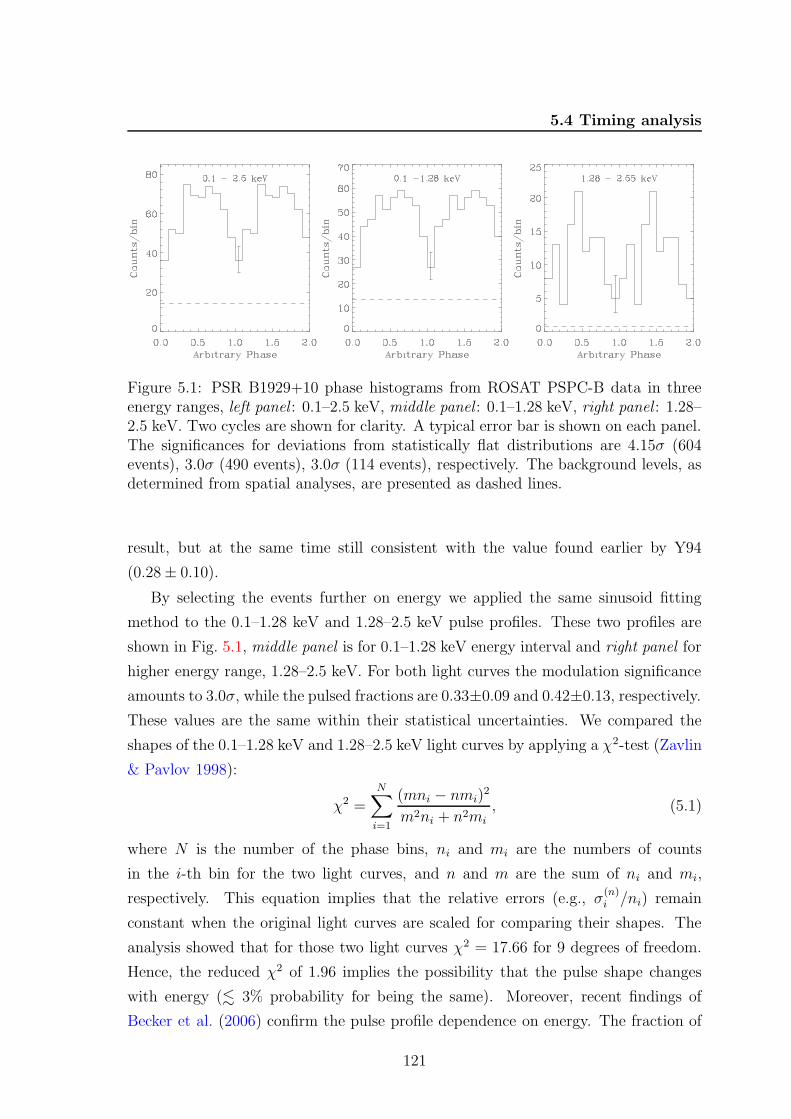
5.4 Timing analysis
Figure 5.1: PSR B1929+10 phase histograms from ROSAT PSPC-B data in threeenergy ranges, left panel : 0.1–2.5 keV, middle panel : 0.1–1.28 keV, right panel : 1.28–2.5 keV. Two cycles are shown for clarity. A typical error bar is shown on each panel.The significances for deviations from statistically flat distributions are 4.15σ (604events), 3.0σ (490 events), 3.0σ (114 events), respectively. The background levels, asdetermined from spatial analyses, are presented as dashed lines.
result, but at the same time still consistent with the value found earlier by Y94
(0.28 ± 0.10).
By selecting the events further on energy we applied the same sinusoid fitting
method to the 0.1–1.28 keV and 1.28–2.5 keV pulse profiles. These two profiles are
shown in Fig. 5.1, middle panel is for 0.1–1.28 keV energy interval and right panel for
higher energy range, 1.28–2.5 keV. For both light curves the modulation significance
amounts to 3.0σ, while the pulsed fractions are 0.33±0.09 and 0.42±0.13, respectively.
These values are the same within their statistical uncertainties. We compared the
shapes of the 0.1–1.28 keV and 1.28–2.5 keV light curves by applying a χ2-test (Zavlin
& Pavlov 1998):
χ2 =N∑
i=1
(mni − nmi)2
m2ni + n2mi, (5.1)
where N is the number of the phase bins, ni and mi are the numbers of counts
in the i-th bin for the two light curves, and n and m are the sum of ni and mi,
respectively. This equation implies that the relative errors (e.g., σ(n)i /ni) remain
constant when the original light curves are scaled for comparing their shapes. The
analysis showed that for those two light curves χ2 = 17.66 for 9 degrees of freedom.
Hence, the reduced χ2 of 1.96 implies the possibility that the pulse shape changes
with energy (. 3% probability for being the same). Moreover, recent findings of
Becker et al. (2006) confirm the pulse profile dependence on energy. The fraction of
121
5. PSR B1929+10 REVISITED IN X-RAYS
pulsed photons derived from the XMM Newton observations in the 0.2–10 keV band
is 32±4%. Within narrower energy ranges 0.2–1.0, 1.0–2.1 and 2.1–10 keV the pulsed
fraction was found at the level of 24 ± 5%, 44 ± 6% and 17 ± 17%, respectively.
At the same time, similar behaviour has been observed by Zavlin & Pavlov (2004,
hereafter ZP04) using the latest XMM-Newton data for another old pulsar emitting
pulsed X-rays, PSR B0950+08. They showed that for this pulsar both the pulse
shape and the pulsed fraction change with energy. In their work the light curve of
PSR B0950+08 is presented in four energy bands: 0.2–0.5, 0.5–1.0, 1.0–5.0 and 0.2–
5.0 keV. The pulsed fractions for these energy ranges are 33±18%, 60±13%, 57±13%
and 41 ± 10%, respectively. For energies above 0.5 keV the pulse profile consists of
two relatively narrow peaks with a high pulsed fraction (≈ 60%), which points to a
non-thermal magnetospherical origin of the X-ray emission. The lower energy light
curve shows a broad single pulse with a lower pulsed fraction of about 33%. ZP04
claim that this energy dependence can be explained by the presence of another, most
likely thermal, component.
5.4.2 ROSAT HRI
For the three long ROSAT HRI observations the timing analysis consisted in ex-
tracting the events from an 11′′ aperture around the centroid of the PSR B1929+10
counterpart and subsequently folding the barycentred event times using an appropri-
ate pulsar ephemeris. The obtained, separately for each observation, pulse profiles
(Fig. 5.2 shows left, middle and right panels for the following time spans of the data
acquisitions 9 Oct–7 Nov 1995, 2–21 Oct 1996 and 13–28 Apr 1997, respectively) have
all a low modulation significance, between 2 and 3σ, although the broad bump can
easily be discerned in all three light curves.
On account of the absolute timing limitations (see Appendix B) we cross-correlated
each of the three HRI profiles with the 0.1–2.5 keV PSPC-B profile. In the cross-
correlation procedure we used the light curves binned into 360 bins. This means
that the width of a single bin corresponds to 629 µs. The obtained shift values were
as follow 0.615, 0.395 and 0.525 for the first, second, and third HRI acquisitions,
respectively. After applying the phase shifts the combination of the three separate
profiles yielded a phase distribution which deviates from a flat distribution at the
3.7σ level (Fig. 5.3, middle panel)1. In this case the sinusoid fitting method yielded a
pulsed fraction of 0.21± 0.05, lower, but still consistent with the PSPC-B value. The
1see Appendix B for the results from a different approach involving event TDB timestamp foldingusing just one single ephemeris for the combination of the three HRI observations
122
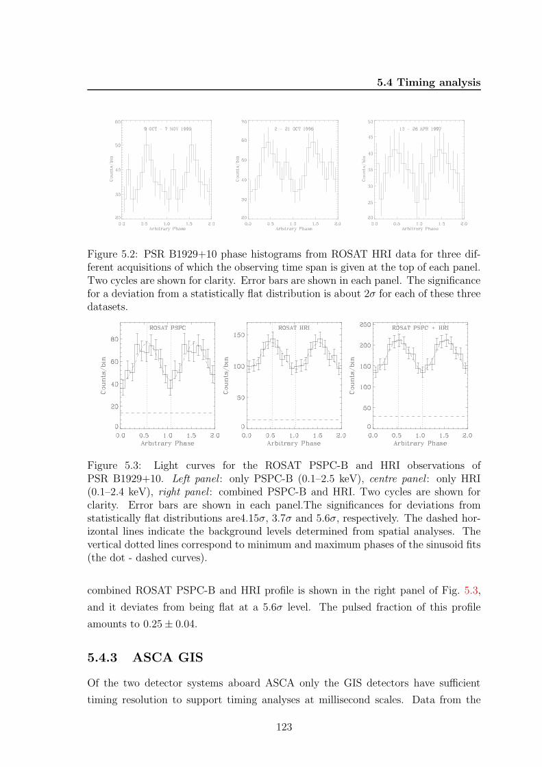
5.4 Timing analysis
Figure 5.2: PSR B1929+10 phase histograms from ROSAT HRI data for three dif-ferent acquisitions of which the observing time span is given at the top of each panel.Two cycles are shown for clarity. Error bars are shown in each panel. The significancefor a deviation from a statistically flat distribution is about 2σ for each of these threedatasets.
Figure 5.3: Light curves for the ROSAT PSPC-B and HRI observations ofPSR B1929+10. Left panel : only PSPC-B (0.1–2.5 keV), centre panel : only HRI(0.1–2.4 keV), right panel : combined PSPC-B and HRI. Two cycles are shown forclarity. Error bars are shown in each panel.The significances for deviations fromstatistically flat distributions are4.15σ, 3.7σ and 5.6σ, respectively. The dashed hor-izontal lines indicate the background levels determined from spatial analyses. Thevertical dotted lines correspond to minimum and maximum phases of the sinusoid fits(the dot - dashed curves).
combined ROSAT PSPC-B and HRI profile is shown in the right panel of Fig. 5.3,
and it deviates from being flat at a 5.6σ level. The pulsed fraction of this profile
amounts to 0.25 ± 0.04.
5.4.3 ASCA GIS
Of the two detector systems aboard ASCA only the GIS detectors have sufficient
timing resolution to support timing analyses at millisecond scales. Data from the
123

5. PSR B1929+10 REVISITED IN X-RAYS
Figure 5.4: The ASCA profiles of PSR B1929+10 in two energy intervals: left panel0.5–5.0 keV (significance 2.7σ, 493 events) and right panel 0.5–2.0 keV (significance3.1σ, 282 events). The dot - dashed curves indicate the sinusoid fitted to the data,while the vertical dotted lines correspond to the minimum and maximum phases ofthe fits. In both panels the horizontal dashed lines indicate the background levelsdetermined from spatial analyses. A typical error bar is shown in each panel. Twocycles are shown for clarity.
high and medium rate telemetry modes were used. The 3.9 ms timing resolution
valid for these rates was sufficiently accurate to sample the pulse period of 227 ms
(see Tab. 5.1). In the spatial analysis a Maximum Likelihood method, similar to that
used for the ROSAT PSPC-B and HRI data, provided the optimum position for the
X-ray counterpart of PSR B1929+10. An extraction radius of 130′′ from this position
was found to optimise the S/N ratio. In the 0.5–5 keV energy interval, the same
as used by WH97, 493 event time tags were barycentred and subsequently folded
through appropriate timing parameters to yield the corresponding pulse profile. This
profile is shown in Fig. 5.4 left panel and deviates from uniformity at a 2.7σ level. The
same broad enhancement is visible as in the ROSAT profiles at softer X-ray energies.
Constraining the energy to the 0.5–2.0 keV interval (282 events), fully overlapping
the ROSAT energy window, yielded a significance of 3.1σ (see Fig. 5.4 right panel).
Note, that in the 2.0–5.0 keV energy range (211 events) the profile is consistent with
being flat, which means that the main contribution to the pulsed fraction comes from
photons with energies lower than 2 keV. The pulsed fractions derived from sinusoid
fitting for the integral (0.5–5 keV) and the ROSAT overlapping (0.5–2.0 keV) energy
ranges are 0.36 ± 0.11 and 0.69 ± 0.18, respectively. The latter value is high, but
because of its large error it is still consistent with the ROSAT numbers, especially
in comparison with the high pulsed fraction of 1.28–2.55 keV PSPC-B light curve
(0.42 ± 0.13).
124

5.4 Timing analysis
Moreover, we can compare our results with those for PSR B0950+08 presented
by ZP04. In the energy band 0.2–5.0 keV, fully overlapping the ASCA band, they
got a pulsed fraction of 41 ± 10%, while for 0.5–1.0 keV band it increased to 60%.
Hence, we argue that the overall situation with respect to the energy dependency of
the pulsed fraction is very similar for both pulsars.
5.4.4 RXTE PCA
Finally, we have analysed RXTE PCA (2–60 keV) data from a 30 ks observation of
PSR B1929+10 (Obs. id. 20156; 21–Nov–1997) obtained in Good Xenon mode, time
tagging each event with a 0.9 µs time resolution. For the timing analysis we used
fasebin program belonging to the FTOOLS1 package to select events from the top layer
of each involved PCU, consequently to barycentre the times of the selected events,
and finally to fold the barycentred event times with an appropriate ephemeris.
Table 5.3: Observed parameters for the radio pulsar B1929+10 based on radio obser-vations made at the Torun Radio Astronomy Observatory. The numbers in paren-theses represent uncertainties in the least significant digits.
Parameter & Value ValueRight Ascension 19h32m13.s924(1)Declination 1059′32.′′44(2)Validity range (MJD) 50608–50959Epoch (MJD TDB) 50700.0Frequency 4.4146591771439(133) HzFirst frequency derivative -2.26596(64) ×10−14 Hz s−1
Second frequency derivative 3.91(84) × 10−24 Hz s−2
The ephemeris used in the folding procedure within fasebin was derived from the
regular pulsar radio timing measurements with 32m Torun Centre for Astronomy ra-
dio telescope. During Torun pulsar timing observations a dual-channel, circular polar-
isation L-band receiving system at frequencies around 1.73 GHz and a 2 x 64 x 3 MHz
pulsar back-end, the Penn State Pulsar Machine 2 (PSPM-2 Konacki et al. 1999), are
used. Data analysis was performed with the standard TEMPO2 software package. To
check occurrence of any timing irregularities broad range of data was used. Time
span covers almost five years, i.e. from Jun, 8th 1997 up to Jun, 1st 2002 and that
1http://heasarc.gsfc.nasa.gov/lheasoft/ftools/2http://pulsar.princeton.edu/tempo
125
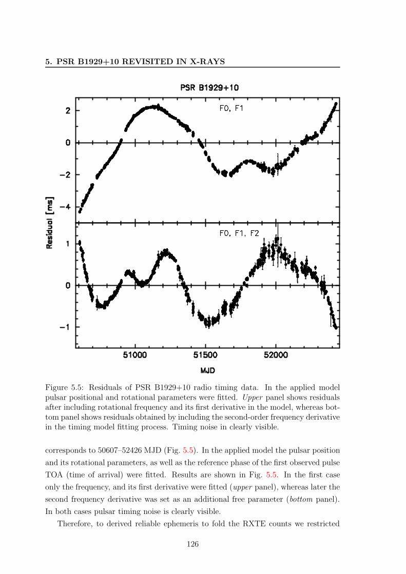
5. PSR B1929+10 REVISITED IN X-RAYS
Figure 5.5: Residuals of PSR B1929+10 radio timing data. In the applied modelpulsar positional and rotational parameters were fitted. Upper panel shows residualsafter including rotational frequency and its first derivative in the model, whereas bot-tom panel shows residuals obtained by including the second-order frequency derivativein the timing model fitting process. Timing noise in clearly visible.
corresponds to 50607–52426 MJD (Fig. 5.5). In the applied model the pulsar position
and its rotational parameters, as well as the reference phase of the first observed pulse
TOA (time of arrival) were fitted. Results are shown in Fig. 5.5. In the first case
only the frequency, and its first derivative were fitted (upper panel), whereas later the
second frequency derivative was set as an additional free parameter (bottom panel).
In both cases pulsar timing noise is clearly visible.
Therefore, to derived reliable ephemeris to fold the RXTE counts we restricted
126

5.5 Comparison of the X-ray and radio profile
Figure 5.6: The same as in bottom panel of Fig. 5.5. The fit was performed for therestricted time span of the data ranging to one year. We got χ2 = 194.48 for 181degrees of freedom, and RMS at the level of 32.15µs.
the time span to one year chosen in a way that the Nov, 21st 1997 (50773 MJD)
fell approximately in the middle of this range. By using TEMPO procedure to fit the
model parameters to selected TOAs the ephemeris in the CGRO format were derived.
Residuals are shown in Fig. 5.6, whereas astrometric and rotational parameters of PSR
B1929+10 obtained from Torun radio timing are presented in Tab. 5.3.
The folding procedure embedded in fasebin resulted in pulse phase histograms for
each of the 256 PHA channels. Unfortunately, in none of the PHA channels or channel
intervals (2–4, 4–8, 8–16, 16–32 keV) significant pulsed emission has been detected.
The lack of detection might be caused by rather short exposure time.
5.5 Comparison of the X-ray and radio profile
Five intensity profiles as a function of radio frequency are shown in Fig. 5.7 (Kramer
et al. (1997) and von Hoensbroech & Xilouris (1997)). They were obtained from
the public data base maintained by the European Pulsar Network1. The radio pulse
profile of PSR B1929+10 consists of two pulses separated by 0.5 in phase: a multi-
component main pulse (for its detailed studies see Weisberg et al. (1999)) and a much
weaker inter pulse (Fig. 5.7). According to the the standard pulsar model (Ruderman
& Sutherland 1975) the integrated pulse width is expected to decrease monotonically
with frequency. This suggests that higher radio frequencies are emitted in the lower
1http://www.mpifr-bonn.mpg.de/pulsar/data/
127

5. PSR B1929+10 REVISITED IN X-RAYS
regions of the pulsar magnetosphere, i.e. closer to the surface of the neutron star.
This phenomenon, called the radius to frequency mapping (RFM), is well established.
The multifrequency observations of pulsars have confirmed the narrowing of pulse pro-
files with frequency. Weisberg et al. (1999) discuss extensively radio multifrequency
observations.
During our (S05) data analysis we did not perform a comparison between radio
and X-ray pulsar light curves, because in the first case (i.e. for the ROSAT and ASCA
data) we did not have radio observations that would have allowed us to obtain the
corresponding radio profiles. Moreover, ROSAT observations do not permit absolute
timing (Appendix B). In the second case, i.e. the RXTE observations, we were
unlucky again. This time we possessed the required radio information, but we did
not find any significant pulsed signal from the high energy data. So far the only
absolutely phase aligned radio and X-ray pulsar profiles are presented in Fig. 7 in
recent publication of Becker et al. (2006). We reproduce this as Fig. 5.8.
The sinusoidal shape of X-ray pulse profile is in sharp contrast to the strongly
peaked radio profile. In B06 the 0.2–10 keV XMM − Newton pulse profile of PSR
B1929+10 is shown together with a radio profile observed at 1.4 GHz. The high energy
profile reveals a significant deviation from a sinusoidal pulse shape. The X-ray pulse
profile consists of at least two pulse peaks: a broader component and a narrow one.
The broader component appears to have substructures that look like two narrower
pulse peaks, not fully resolved even in the XMM − Newton data. The second main
component, i.e. the narrow peak, appears at energies ≥ 1 keV. Some indication of
such behaviour has been already shown by us in the ROSAT PSPC-B data (Fig. 5.1,
left panel), but with low statistics. Moreover, this narrow X-ray component appears
to be slightly phase shifted from the location of the main radio peak, although both
components overlap reasonably well in phase.
5.6 Spectral analysis
By studying the X-ray spectrum and temporal modulation of this and other similar
objects, we hope to learn about the origin of the X-ray emission. If the spectrum is
thermal and the projected area is small relative to that of the star, we conclude that
there is a “hot-spot” on the neutron star surface. If the spectrum is non-thermal, it
might be an indication of magnetospheric emission.
In the spectral analysis we first derived the total (= pulsed plus DC) number
of counts assigned to the X-ray counterpart of PSR B1929+10 in several narrow
128

5.6 Spectral analysis
Table 5.4: Fits to the combined ROSAT and ASCA spectrum in the energy range0.1–10 keV.
Parameter Power Law Fit
Ca 6.41+0.4−0.4 × 10⁻⁵
α 2.54+0.12−0.13
NH 9.8+1.4−1.0 × 1020 cm−2
χ2ν/ν 1.146/27
Parameter Double Black-Body Fit
Cb1 0.0117+0.0017
−0.0018
kT1 0.176+0.004−0.004 keV
Cb2 7.879+1.32
−1.26 × 10⁻⁵
kT2 0.595+0.02−0.03 keV
NH 4.43+2.08−1.12 × 1020 cm−2
χ2ν/ν 1.132/25
a Normalisation at 1 keV (ph cm−2 s−1 keV−1)
b BB normalisation (ph cm−2 s−1 keV−3)
energy slices using a spatial (MLR) analysis which takes into account the presence of
nearby sources. We applied this approach to the ROSAT PSPC-B (20 energy bins
in the interval 0.1–2.5 keV) and ASCA GIS 2+3 (10 energy bins in the interval 0.5–
10 keV) data. In contrary to WH97 we chose for ASCA the GIS data, because the
GIS sensitivity is higher than the SIS sensitivity for energies beyond ∼ 5 keV and
because of uncertainties in the SIS efficiency for energies below 1 keV. In the combined
ROSAT PSPC-B and ASCA GIS 2+3 spectral fits we used the latest upgrades for
the response matrices and we took into account the vignetting corrections for the 3.′7
off-axis ASCA observation.
The spectral models fitted to the combined data set consist of an absorbed single
power law (PL), an absorbed single black-body, an absorbed black-body plus power
law and an absorbed double black-body (BB). The best fits were obtained for an
absorbed single power law (Fig. 5.9, upper panel) and an absorbed double black-body
model (Fig. 5.9, lower panel). The fit results for these two cases, each with a free
hydrogen column density, are shown in Table 5.4.
We found that the PL model fits tha data almost as well as the double BB model,
yielding the photon index α = 2.54+0.12−0.13 and the absorbing hydrogen column density
129

5. PSR B1929+10 REVISITED IN X-RAYS
NH= 9.8+1.4−1.0×1020 cm−2. Then the derived flux f in the range 0.1–10 keV amounts to
(6.05±0.49)×10−13 erg cm−2 s−1. Together with a distance d of 331±10 pc adopted
from (Brisken et al. 2002) it implies an isotropic X-ray luminosity, LX(0.1−10 keV) =
4πd2f, of (7.9 ± 0.8) × 1030 erg s−1. From recent VLBA parallax measurements,
Chatterjee et al. (2004) obtained an even larger distance of 361+10−8 pc, which would
change our 0.1–10 keV isotropic luminosity to (9.4 ± 0.9) × 1030 erg s−1. The 0.1–
10 keV isotropic X-ray luminosity represents 2× 10⁻³ of the spin-down power E (see
Table 1) of PSR B1929+10 for the 331 pc distance estimate. For the 0.1–2.4 keV
band we obtain an isotropic X-ray luminosity of (7.1 ± 0.7) × 1030 erg s−1 which
translates to LX(0.1 − 2.4 keV)/E ratio of 1.8 × 10⁻³. This value is compatible with
e.g. the (LX(0.1 − 2.4 keV), E) empirical relation found by Seward & Wang (1988):
logLX = 1.39logE − 16.6 and later confirmed by Verbunt et al. (1996): LX ≈ 10−3E.
In the case of the double black-body model we are dealing with two different
thermal X-ray components with temperatures 2.0+0.05−0.05×10⁶ K and 6.9+0.23
−0.35×10⁶ K for
T1 and T2, respectively. For the characteristic age of PSR B1929+10 (τ ' 3.1 Myr)
cooling models predict a surface temperature of the neutron star to be ≤ 105 K,
much too low to be responsible for the observed X-ray spectrum of PSR B1929+10.
However, a plausible explanation could be that the observed X-ray radiation originates
from a heated polar cap characterized by two different thermal components (see e.g.
Cheng & Zhang 1999). The simultaneous double BB fit to the ROSAT and ASCA
data implies emission luminosities of L1 = (1.56 ± 0.25) × 1030 erg s−1 and L2 =
(1.47 ± 0.25) × 1029 erg s−1 for T1 and T2 components, respectively. The derived
luminosities allow us to calculate the areas A of the emitting regions responsible for
the detected X-rays. Following the simple estimations for the area A = LX/σT 4 we
obtain the following numbers: A1 = 1.72×109 cm2, A2 = 1.13×106 cm2 for the 2 MK
and 7 MK black-body components, respectively. The A1 and A2 values as measured
at the NS surface have to be corrected for the gravitational redshift (gr) relating the
areas derived from observations and the intrinsic emitting areas on the star. The
gravitational redshift is described by the relation
gr = (1 + z)−1 =
[
1 − 2GM
c2RNS
]1/2
, (5.2)
and for the canonical values M = 1.4M and RNS = 10 km it amounts to 0.766.
Because Aint = Ag2r we obtained Aint,1 = 1.01× 109 cm2 and Aint,2 = 6.69× 105 cm2.
The derived areas correspond to only ∼ 0.8× 10⁻⁴ and ∼ 5.3× 10⁻⁸ of the stellar
surface, assuming RNS = 10 km. On the other hand, we also compare the emitting
130

5.6 Spectral analysis
areas to the canonical polar cap size. It is defined by the locus of the last closed dipole
field line (e.g. Michel 1991). For the parameters of PSR B1929+10 the intrinsic polar
cap area is
APC =2π2R3
NS
cP= 2.9 × 109 cm2, (5.3)
where P is the pulsar period, and RNS was assumed to be 10 km. The derived Aint,1 ,
and Aint,2 values are smaller by only a factor of 3 and significantly smaller (∼ 2×10⁻⁴)
than APC area in the low- and high-temperature component case, respectively. This
shows that for thermal emission model, the X-ray emission area of PSR B1929+10 is
roughly consistent with the conventional size of a heated polar cap. The discrepancy
between Aint,1 and APC of the factor of 3 can be realistic if we consider the complicated
distribution of the magnetic field on the surface of a neutron star, distortion of the
surface black-body spectrum due to propagation of the radiation through a pulsar
magnetosphere and the beam solid angle.
In conclusion, for thermal interpretation the result means that the observed X-ray
emission does not have its origin in the cooling emission from the entire surface of
the neutron star, because the implied temperature is unexpectedly high for such an
old pulsar. Furthermore, the derived emitting area is extremely small in comparison
to the NS surface area.
5.6.1 High value of the neutral hydrogen column density
The NH value obtained from the double BB fit is about four and that obtained from
the PL-fit about eight times larger that the NH value used by Y94 and WH97. In
both cases the newly derived column densities are consistent with the updated (radio)
distance determined by Brisken et al. (2002) from VLBA data, and the hydrogen dis-
tribution measured in the direction of the pulsar (Frisch & York 1983). Additionally,
as Pavlov et al. (1996) have already mentioned, values of NH obtained from the direct
measurements of stars in the neighbourhood of the pulsar are rather controversial.
They differ from . 1019 up to 1021 cm−2. This behaviour is illustrated in Fig. 5.10.
The presented data, gathered in Tab. 5.5, were obtained using the ISM hydrogen Col-
umn Density Search Tool 1 available on the Extreme Ultraviolet Explorer (EUVE) web
page. For further discussion we will concentrate on only five out of the ten selected
sources from the EUVE database nearest to PSR B1929+10. These are: σ Aql, ε Del,
o Her, WD1910+047 and ES Vul. The first two sources are approximately halfway
1http://stdatu.stsci.edu/euve/ism/ismform.html
131

5. PSR B1929+10 REVISITED IN X-RAYS
Table 5.5: The parameters of ten EUVE sources placed in the pulsar direction asderived by the ISM hydrogen Column Density Search Tool.
HD Name Name l b da NHb
HD180968 ES Vul 56.4 4.9 408.0 20.99♠
— WD1910+047 39.7 -2.5 210.0 19.00†
HD170740 — 21.1 -0.5 279.0 21.04♠
HD163472 V2052 Oph 27.2 12.6 349.0 21.12♠
HD166014 o Her 55.2 21.6 200.0 19.65‡
HD161056 — 18.7 11.6 263.0 21.20♠
HD164284 66 Oph 31.0 13.4 184.0 20.90F
HD162094 — 59.5 27.3 320.0 20.50♣
HD195810 ε Del 55.4 -16.6 150.0 19.52‡
HD185507 σ Aql 43.3 -8.1 140.0 21.01♣
a Distance (in parsecs) between the star and the Earth.
b Reference ♠ Diplas & Savage (1994), † Paerels & Heise (1989), ‡ Welsh et al.(1991), F Bohlin et al. (1983), ♣ Brown et al. (1991).
between the Earth and the pulsar, whereas the third and fourth source are at a two-
third way and the last source is about 80 pc farther from the observer than the pulsar
is. The dependence of the logarithm of the interstellar hydrogen column densities
on the distances for all ten sources, as well as for PSR B1929+10, is shown in the
upper panel of Fig. 5.10. It is quite clear that, in some cases, even if the source is not
very far away the logarithm of NH can be as large as 21, as it happens for example
for σ Aql. On the contrary, ε Del being roughly at the same distance as σ Aql, or
o Her and WD1910+047 distant only about 50 pc from σ Aql all do have rather small
values of the logarithm of NH. This suggests that the interstellar medium is very
patchy in that direction. The spatial distribution of all sources in the Galactic coor-
dinates (l, b) is shown in the bottom panel of Fig. 5.10. For the pulsar and the five
chosen stars their names and the values of their distances and NH (in brackets) are
presented. We can distinguish two regions. The first region encircles the surface with
borders determined by the positions of the following sources WD1910+047, ε Del and
o Her. For this region, which is placed around 150–200 pc away, the average value
of neutral hydrogen column density is at the level of 2.4 × 1019 cm−2. The second
region, overlapping the first one, seems to be much smaller and elongates along the
line connecting σ Aql, PSR B1929+10 and ES Vul. The average NH is at the level of
9.92 × 1020 cm−2 here and it is about 40 times larger than that of region one.
132
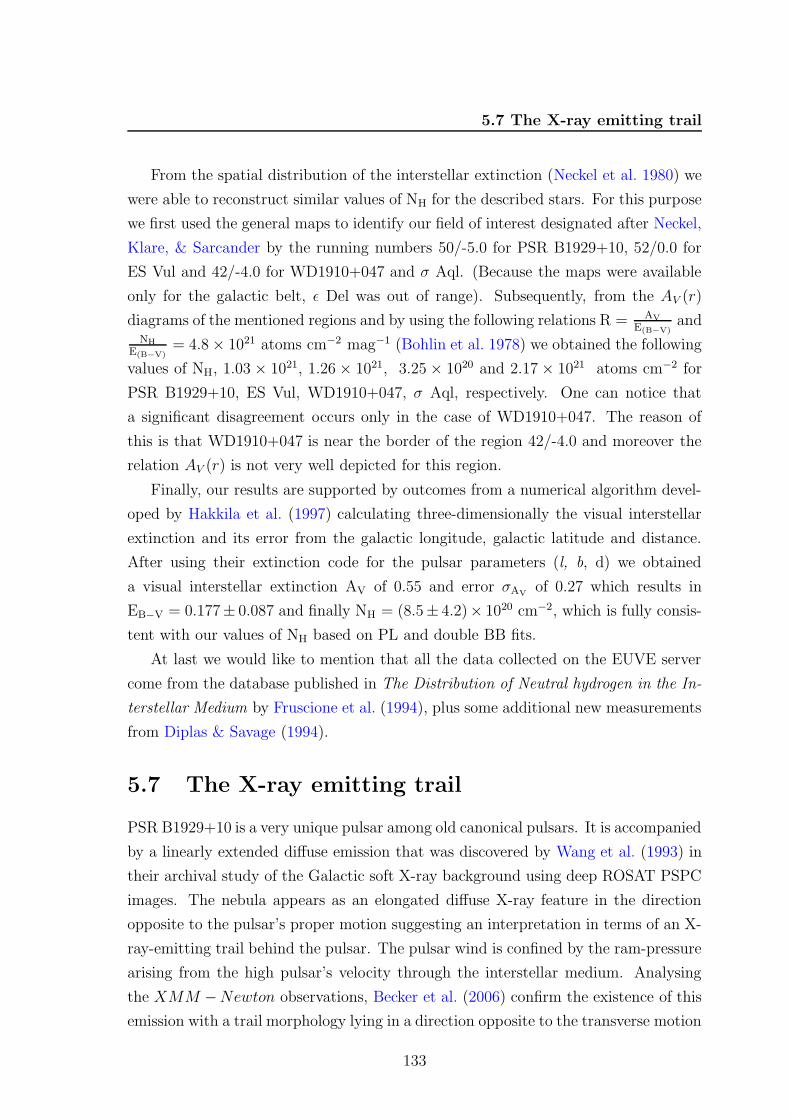
5.7 The X-ray emitting trail
From the spatial distribution of the interstellar extinction (Neckel et al. 1980) we
were able to reconstruct similar values of NH for the described stars. For this purpose
we first used the general maps to identify our field of interest designated after Neckel,
Klare, & Sarcander by the running numbers 50/-5.0 for PSR B1929+10, 52/0.0 for
ES Vul and 42/-4.0 for WD1910+047 and σ Aql. (Because the maps were available
only for the galactic belt, ε Del was out of range). Subsequently, from the AV (r)
diagrams of the mentioned regions and by using the following relations R = AV
E(B−V)and
NH
E(B−V)= 4.8 × 10²¹ atoms cm−2 mag−1 (Bohlin et al. 1978) we obtained the following
values of NH, 1.03 × 10²¹, 1.26 × 10²¹, 3.25 × 10²⁰ and 2.17 × 10²¹ atoms cm−2 for
PSR B1929+10, ES Vul, WD1910+047, σ Aql, respectively. One can notice that
a significant disagreement occurs only in the case of WD1910+047. The reason of
this is that WD1910+047 is near the border of the region 42/-4.0 and moreover the
relation AV (r) is not very well depicted for this region.
Finally, our results are supported by outcomes from a numerical algorithm devel-
oped by Hakkila et al. (1997) calculating three-dimensionally the visual interstellar
extinction and its error from the galactic longitude, galactic latitude and distance.
After using their extinction code for the pulsar parameters (l, b, d) we obtained
a visual interstellar extinction AV of 0.55 and error σAVof 0.27 which results in
EB−V = 0.177± 0.087 and finally NH = (8.5± 4.2)× 1020 cm−2, which is fully consis-
tent with our values of NH based on PL and double BB fits.
At last we would like to mention that all the data collected on the EUVE server
come from the database published in The Distribution of Neutral hydrogen in the In-
terstellar Medium by Fruscione et al. (1994), plus some additional new measurements
from Diplas & Savage (1994).
5.7 The X-ray emitting trail
PSR B1929+10 is a very unique pulsar among old canonical pulsars. It is accompanied
by a linearly extended diffuse emission that was discovered by Wang et al. (1993) in
their archival study of the Galactic soft X-ray background using deep ROSAT PSPC
images. The nebula appears as an elongated diffuse X-ray feature in the direction
opposite to the pulsar’s proper motion suggesting an interpretation in terms of an X-
ray-emitting trail behind the pulsar. The pulsar wind is confined by the ram-pressure
arising from the high pulsar’s velocity through the interstellar medium. Analysing
the XMM −Newton observations, Becker et al. (2006) confirm the existence of this
emission with a trail morphology lying in a direction opposite to the transverse motion
133

5. PSR B1929+10 REVISITED IN X-RAYS
of the pulsar (µα = 94.09±0.11 and µδ = 42.99±0.16 mas yr−1, V⊥ = 177+4−5 km s−1;
Chatterjee et al. (2004)). The XMM − Newton maps, see Fig. 5.11, show clearly
diffuse extended emission at the position of the putative X-ray trail seen already in the
ROSAT PSPC data (Wang et al. 1993). Contour lines, obtained from a reanalysis
of the ROSAT PSPC and HRI observations (A. S lowikowska), are overlaid on the
XMM − Newton maps (W. Becker). Because of the instrument characteristics and
the dependence on the source spectrum, it is much harder to detect the trail structure
in the HRI data. It was possible only after applying an adaptive kernel smoothing
procedure. Then the resulting structure becomes visible and matches with the shape
of the trail seen in ROSAT PSPC and MXX − Newton images. The trail spectrum
is non-thermal and characterised by a power law photon index of ∼ 2 (B06). It is
interpreted as synchrotron emission in the shock between the pulsar wind and the
surrounding medium.
Radio data from the Effelsberg 11 cm radio continuum survey show an elongated
feature that roughly coincides with the X-ray trail (Fig. 5.12, left). Three not fully
resolved radio sources seen in the NRAO VLA Sky Survey (NVSS) survey data at 1.4
GHz match with part of the elongated radio feature seen at 11 cm (Fig. 5.12, right).
The result obtained from the X-ray trail along with the possible discovery of its radio
counterpart are exciting (B06). Follow-up radio observations of the trail region at
different wavelengths are currently scheduled for fall 2006 in order to further constrain
its existence and, if detected, provide polarisation information and the spectral index
in the radio regime.
5.8 Summary and conclusions
Our revisited analysis of X-ray data of PSR B1929+10 from ROSAT, ASCA and
RXTE observations yielded an improved timing signal at soft X-rays of 5.6σ for
the combined ROSAT PSPC-B/HRI pulse profile, and a non-detection for energies
beyond ∼ 2 keV (RXTE PCA). Analysing the pulse profiles at soft X-rays (ROSAT
PSPC-B) in two different energy bands yielded the pulsed fractions 0.33 ± 0.09 in
the 0.1–1.28 keV band, 0.42± 0.13 in the 1.28–2.5 keV band, and 0.69± 0.18 for the
0.5–2 keV ASCA GIS band.
A spectral analysis of the combined ROSAT/ASCA data in the 0.1–10 keV en-
ergy range indicated that both an absorbed power law (non-thermal) model and an
absorbed double black-body model provide an adequate description of the observed
X-ray spectrum. For the double BB model a plausible explanation could be that
134

5.8 Summary and conclusions
the observed X-ray radiation originates from a heated polar cap characterised by two
different thermal components (Cheng & Zhang 1999). The derived hydrogen column
densities (NH) are in both cases much larger than the value used in previous X-ray
studies. However, the newly determined NH values are more consistent with the
updated (increased) distance to PSR B1929+10 in combination with the measured
hydrogen distribution in the direction of the pulsar.
A recent observation performed with the XMM-Newton satellite (B06) allows to
validate results obtained by S lowikowska et al. (2005b). Improved statistic shows that
the pulsar’s X-ray spectrum is best described by a single power law model with pho-
ton index of 2.72+0.12−0.09 (being in good agreement with our result, see Tab. 5.4), whereas
the pure thermal emission spectrum consisting of two black-body components is re-
garded as rather unlikely. Furthermore, Becker et al. (2006) show that a combination
of thermal and non-thermal spectral model (BB+PL) is possible, but the inferred
contribution to the flux from the thermal emission of heated polar caps is not more
than 7%. Noteworthy is the fact, that all spectral models considered by Becker et al.
(2006) give, in comparison with values used by Y94 and WH97, a higher value of NH,
e.g. (0.35± 0.11)× 1021 cm−2 for double BB fit, and even (1.6± 0.2)× 1021 cm−2 for
a single PL case. Thus, the high value of NH obtained by S lowikowska et al. (2005b)
have been confirmed. Besides giving the constrains for the high energy pulsar emis-
sion, the large collecting area of the XMM − Newton satellite has allowed, for the
first time, spectral analysis of the emission from the pulsar’s X-ray trail (B06).
S lowikowska et al. (2005b) performed timing and spectral analyses for PSR B1929+10,
one of the oldest (∼107 years) of the ordinary pulsars detected in X-rays, using archival
ROSAT, ASCA and RXTE data. Pulsed emission was detected at more than five
sigma level for the combined ROSAT PSPC-B and previously unpublished HRI data.
Our pulse profile is in agreement with that obtained by Yancopoulos et al. (1994)
(ROSAT PSPC-B) but now with better statistics. The pulsed fraction in the ROSAT
X-ray band is 0.25±0.04. The pulsed signal has also been detected in the ASCA GIS
data (0.5–5 keV) with a similar pulsed fraction that amounts to 0.36±0.11. No signif-
icant timing signal is found in the RXTE PCA data (> 2 keV). The most important
result from this work is derived from the spectral analysis. We found that the com-
bined ROSAT PSPC-B and ASCA GIS spectrum can satisfactorily be described by
a power law as well as by a double black-body model but not by a single black-body
model or black-body plus power law model, as was presented earlier by Yancopoulos
et al. (1994) and Wang & Halpern (1997) for ROSAT and ASCA data, respectively.
In both cases the derived NH value is higher than that adopted in earlier works, but
135

5. PSR B1929+10 REVISITED IN X-RAYS
our result is fully consistent with the larger pulsar distance estimates (Brisken et al.
2002; Chatterjee et al. 2004) in combination with the hydrogen distribution measured
in the direction of the pulsar (Frisch & York 1983). Our results have been recently
verified by Becker et al. (2006) who used the XMM − Newton observations.
136

5.8 Summary and conclusions
0.0 0.2 0.4 0.6 0.8 1.00.00.2
0.4
0.6
0.81.0
Inte
nsity
(a.
u.)
x15
1.410 GHz
0.0 0.2 0.4 0.6 0.8 1.00.00.2
0.4
0.6
0.8
1.0
Inte
nsity
(a.
u.)
x15
1.710 GHz
0.0 0.2 0.4 0.6 0.8 1.00.00.2
0.4
0.6
0.8
1.0
Inte
nsity
(a.
u.)
x15
4.850 GHz
0.0 0.2 0.4 0.6 0.8 1.00.00.2
0.4
0.6
0.8
1.0
Inte
nsity
(a.
u.)
x5
8.500 GHz
0.0 0.2 0.4 0.6 0.8 1.0Phase
0.00.2
0.4
0.6
0.8
1.0
Inte
nsity
(a.
u.)
x5
10.055 GHz
Figure 5.7: Normalised total intensity of PSR B1929+10 as a function of radio fre-quency (Kramer et al. (1997) and von Hoensbroech & Xilouris (1997)). Data weretaken from the public data base maintained by the European Pulsar Network. Thedotted lines show the same profile magnified by a few times to better visualise theweak inter pulse component around 0.8 phase. Profiles were aligned with the maxi-mum at 1.41 GHz.
137

5. PSR B1929+10 REVISITED IN X-RAYS
Figure 5.8: Upper : integrated pulse profile of PSR B1929+10 as observed in the 0.2–10 keV band with the XMM − Newton satellite. Bottom: the radio profile at 1.4GHz obtained with the Jodrell Bank radio observatory and plotted on a logarithmicscale to better characterise the weak inter pulse component. Both profiles are phasealigned. Two phase cycles are shown for clarity. [Becker et al. (2006)]
138
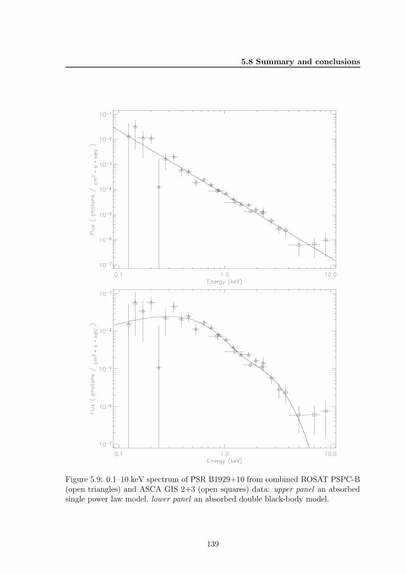
5.8 Summary and conclusions
Figure 5.9: 0.1–10 keV spectrum of PSR B1929+10 from combined ROSAT PSPC-B(open triangles) and ASCA GIS 2+3 (open squares) data: upper panel an absorbedsingle power law model, lower panel an absorbed double black-body model.
139
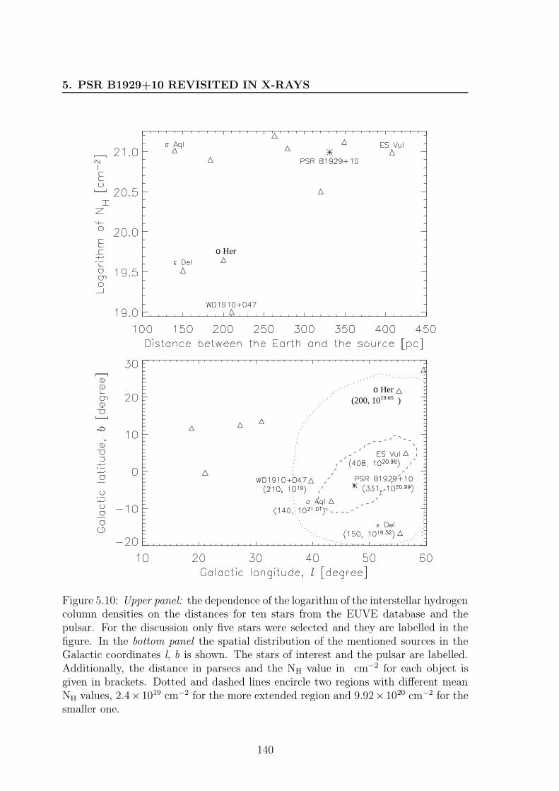
5. PSR B1929+10 REVISITED IN X-RAYS
19.65(200, 10 )Herο
ο Her
Figure 5.10: Upper panel: the dependence of the logarithm of the interstellar hydrogencolumn densities on the distances for ten stars from the EUVE database and thepulsar. For the discussion only five stars were selected and they are labelled in thefigure. In the bottom panel the spatial distribution of the mentioned sources in theGalactic coordinates l, b is shown. The stars of interest and the pulsar are labelled.Additionally, the distance in parsecs and the NH value in cm−2 for each object isgiven in brackets. Dotted and dashed lines encircle two regions with different meanNH values, 2.4× 1019 cm−2 for the more extended region and 9.92× 1020 cm−2 for thesmaller one.
140

5.8 Summary and conclusions
Figure 5.11: PSR B1929+10 and its environment as seen in the 0.2–10.0 keV energyband by MXX-Newton’s detectors. Contour lines from the ROSAT PSPC and HRIimage are overlaid in the left and right panel, respectively. The angular resolutionof the ROSAT detectors are 25” in the PSPC and 5” in the HRI, respectively, whilethat of XMM − Newton is 15”. [Maps W. Becker; contours A. S lowikowska]
Figure 5.12: Left: contour lines from the ROSAT PSPC overlaid on part of theEffelsberg 11 cm radio map. Right: contour lines from the ROSAT HRI overlaid onpart of the 1.4 GHz NRAO VLA Sky Survey (NVSS) image. [Becker et al. (2006)]
141

Chapter 6
Closing remarks
Pulsar astronomy is truly a multiwavelength field. Neutron stars as rotation-powered
pulsars are now observed across the entire electromagnetic spectrum from radio waves
to gamma rays. In this thesis the results of radio, optical, and X-ray studies of three
classical pulsars are presented. By arranging the observations, followed by data re-
duction and analysis we attempted to broaden our knowledge of these objects. Con-
clusions and possible implications from this work were discussed in the corresponding
chapters, and they will not be fully repeated here. Below a brief summary of the
results is given, as well as future projects are discussed.
First two chapters are dedicated to the Crab pulsar. One might expect that
after 38 years of extensive studies we should know almost everything about this
source. However, it turned out not to be the case and it is still worth to point the
telescopes at this source. In Chapter 1 we presented our discovery of giant radio
pulses (GRPs) occurring at the phases of high frequency component (HFCs, Jessner
et al. (2005); S lowikowska et al. (2005a)). Our finding challenges the idea that GRPs
are aligned exclusively with the main pulse (MP) and the inter pulse (IP). It weakens
the hypothesis that GRP phenomenon is somehow connected with the non-coherent
high energy emission. In order to study the evolution of giant pulses with frequency,
as well as to investigate their fluxes, time structures, and polarisation we have applied
recently for the observing time at the Effelsberg telescope. We propose observations
of the Crab pulsar at 14.6 and 23 GHz to study spectral and polarimetric properties
of GRPs at the IP and HFCs phases, and to search for possible new components in its
average radio profile. Simultaneous observations at the lower frequencies of 0.6, 2.2
and 4.8 GHz will be performed at the 64-m radio telescope in Kalyazin (Russia). Such
observations will allow to investigate the physical relation between HFCs and regular
MP and IP at lower frequencies and compare their properties in a broad frequency
range. It might also provide new constraints to the location and configuration of
142

emission regions in the Crab pulsar. This project is going to be performed by the end
of 2006.
Polarisation measurements of pulsars and of their synchrotron nebulae provide
deep insights into the highly magnetised relativistic environment of young rotating
neutron stars and allow to test current magnetospheric and wind models. Apart from
the radio band, polarisation is best measured in the optical. Chapter 2, the most
extensive one, describes the results of our polarimetric campaign of the Crab pulsar
at Nordic Optical Telescope with OPTIMA. Our results reveal complex behaviour of
polarisation degree and position angle of rotational phase. These high-quality results
with time resolution of about 30 µs will certainly stimulate a significant revision of
major pulsar models. Pulsar polarisation characteristics obtained with such high time
resolution establish the OPTIMA instrument with the rotating polarisation filter as
a very power full polarisation system.
We decided to extend our polarimetric studies to other pulsars. PSR B0540-69 is
one of the brightest optical pulsars and similar to the Crab pulsar. It is embedded
in a synchrotron nebula visible at optical wavelengths. We successfully applied for
the HST time to observe PSR B0540-69 and its compact nebula with the Advanced
Camera for Surveys (ACS) and the Wide Field Channel (WFC) detector using UV
and visual polarisation filters. Thanks to the superb angular resolution of ACS, these
observations will allow us to resolve the pulsar from its nebular background, providing
the first firm measure of the pulsar phase-averaged polarisation. Thus the number of
pulsars with measured optical polarisation will hopefully increase. The observations
will also provide the first detailed polarisation map of the nebula, including the jet and
the torus seen in previous WFPC2 images. Our proposal has been already approved
and we expect that the observations will be performed in Winter 2006.
To obtain the high time resolution photometry of the second and third brightest
optical pulsars - PSR B0540-69 and PSR B0833-45 (Vela) - we are preparing an
observational campaign at Southern African Large Telescope. These pulsars are of
average magnitude of V ∼ 22.7 and 23.6, respectively, thus the large collecting power
of SALT is essential to conduct the measurements. For our purpose we propose to
use OPTIMA as a guest instrument. The immediate results of such measurements
would be: optical light curves of PSR B0540-69 and Vela with very high statistical
accuracy and the first determination of the phase dependent linear polarisation of
these pulsars.
Chapters 3 and 4 present the X-ray data analysis and results of PSR B0540-69
and PSR B1929+10, respectively. In the first case, despite of long exposure time
143
6. CLOSING REMARKS
the results are not of high significance. Yet, the interesting piece of information we
managed to obtain is the total spectrum of this object extending, for the first time, up
to 200 keV. Chapter 4 deals with the archive X-ray data of one of the oldest observed
X-ray pulsar, PSR B1929+10. Neutron stars are born with temperatures of more
than 1012 K during the collapse of massive stars. They start to cool down directly
after they are born. The cooling process strongly depends on the physical properties
of superdense matter inside them. X-ray observations of neutron stars have already
shown that their radiation may have three different origins: (1) whole surface is so hot
that it emits thermal X-rays; (2) charged particles moving in strong magnetic field
produce non-thermal X-rays; (3) thermal X-rays come from the reheated polar caps.
Our reanalysis of the archival data of PSR B1929+10 attempted to identify possible
origin of its X-rays. Unfortunately, we were not able to distinguish explicitly between
the thermal and non-thermal source of emission (S lowikowska et al. 2005b). However,
our non-thermal model seems to be confirmed by recent XMM-Newton observations
(Becker et al. 2006). These results suggest that the observed X-ray emission of this
pulsar is due to the magnetospheric emission and not due to hot polar caps. The
heating of the polar surface regions by particle bombardment is not efficient enough
to produce significant thermal X-ray component.
Pulsar phenomenon, nearly forty years after the discovery by Jocelyn Bell, is still
not well understood, and therefore more observations with sensitive instruments in
all energy domain are needed.
144
Appendix A
OPTIMA data files
For the main data analysis 83 out of 160 files were selected as acceptable for analysis
(about the selection criteria see Sec. 3.2.3). First part of the file name contains object
name plus additionally abbreviated name of used filters, in this case it were infrared
and rotating polarisation filters, second part of the file name contains the date and
the UTC time when the data acquisition started. Number of files given in the table
are hereafter used as an arbitrary file number, see e.g. Fig. 3.9 or 3.10.
145

A. OPTIMA DATA FILES
Table A.1: Log of good data file namesNo. File Name No. File Name
0 Crab-IR+Pol 25Nov2003 (25-11-2003 23-02-42) 42 Crab-IR+Pol 26Nov2003 (26-11-2003 23-21-48)
1 Crab-IR+Pol 25Nov2003 (25-11-2003 23-12-45) 43 Crab-IR+Pol 26Nov2003 (26-11-2003 23-31-51)
2 Crab-IR+Pol 25Nov2003 (25-11-2003 23-22-48) 44 Crab-IR+Pol 26Nov2003 (26-11-2003 23-41-54)
3 Crab-IR+Pol 25Nov2003 (25-11-2003 23-32-51) 45 Crab-IR+Pol 26Nov2003 (26-11-2003 23-51-57)
4 Crab-IR+Pol 25Nov2003 (25-11-2003 23-42-54) 46 Crab-IR+Pol 26Nov2003 (27-11-2003 00-02-01)
5 Crab-IR+Pol 25Nov2003 (25-11-2003 23-52-57) 47 Crab-IR+Pol 26Nov2003 (27-11-2003 00-12-04)
6 Crab-IR+Pol 25Nov2003 (26-11-2003 00-03-01) 48 Crab-IR+Pol 26Nov2003 (27-11-2003 00-22-07)
7 Crab-IR+Pol 25Nov2003 (26-11-2003 00-13-04) 49 Crab-IR+Pol 26Nov2003 (27-11-2003 00-32-10)
8 Crab-IR+Pol 25Nov2003 (26-11-2003 00-23-07) 50 Crab-IR+Pol 26Nov2003 (27-11-2003 00-42-13)
9 Crab-IR+Pol 25Nov2003 (26-11-2003 00-33-10) 51 Crab-IR+Pol 26Nov2003 (27-11-2003 00-52-16)
10 Crab-IR+Pol 25Nov2003 (26-11-2003 00-43-58) 52 Crab-IR+Pol 26Nov2003 (27-11-2003 01-03-27)
11 Crab-IR+Pol 25Nov2003 (26-11-2003 00-54-01) 53 Crab-IR+Pol 26Nov2003 (27-11-2003 01-13-30)
12 Crab-IR+Pol 25Nov2003 (26-11-2003 01-04-04) 54 Crab-IR+Pol 26Nov2003 (27-11-2003 01-23-33)
13 Crab-IR+Pol 25Nov2003 (26-11-2003 01-14-07) 55 Crab-IR+Pol 26Nov2003 (27-11-2003 01-33-36)
14 Crab-IR+Pol 25Nov2003 (26-11-2003 01-24-10) 56 Crab-IR+Pol 26Nov2003 (27-11-2003 01-43-39)
15 Crab-IR+Pol 25Nov2003 (26-11-2003 01-34-13) 57 Crab-IR+Pol 26Nov2003 (27-11-2003 01-53-42)
16 Crab-IR+Pol 25Nov2003 (26-11-2003 01-44-16) 58 Crab-IR+Pol 26Nov2003 (27-11-2003 02-03-45)
17 Crab-IR+Pol 25Nov2003 (26-11-2003 01-54-19) 59 Crab-IR+Pol 26Nov2003 (27-11-2003 02-13-48)
18 Crab-IR+Pol 25Nov2003 (26-11-2003 02-04-22) 60 Crab-IR+Pol 26Nov2003 (27-11-2003 02-41-53)
19 Crab-IR+Pol 25Nov2003 (26-11-2003 02-14-25) 61 Crab-IR+Pol 26Nov2003 (27-11-2003 02-52-44)
20 Crab-IR+Pol 25Nov2003 (26-11-2003 02-24-28) 62 Crab-IR+Pol 26Nov2003 (27-11-2003 03-02-47)
21 Crab-IR+Pol 25Nov2003 (26-11-2003 03-05-20) 63 Crab-IR+Pol 26Nov2003 (27-11-2003 03-08-17)
22 Crab-IR+Pol 25Nov2003 (26-11-2003 03-15-59) 64 Crab-IR+Pol 26Nov2003 (27-11-2003 03-18-49)
23 Crab-IR+Pol 25Nov2003 (26-11-2003 03-52-43) 65 Crab-IR+Pol 26Nov2003 (27-11-2003 03-28-52)
24 Crab-IR+Pol 25Nov2003 (26-11-2003 04-02-46) 66 Crab-IR+Pol 26Nov2003 (27-11-2003 03-38-55)
25 Crab-IR+Pol 25Nov2003 (26-11-2003 04-13-21) 67 Crab-IR+Pol 26Nov2003 (27-11-2003 03-48-58)
26 Crab-IR+Pol 25Nov2003 (26-11-2003 04-23-24) 68 Crab-IR+Pol 26Nov2003 (27-11-2003 03-59-01)
27 Crab-IR+Pol 25Nov2003 (26-11-2003 04-33-27) 69 Crab-IR+Pol 26Nov2003 (27-11-2003 04-09-04)
28 Crab-IR+Pol 25Nov2003 (26-11-2003 04-43-30) 70 Crab-IR+Pol 26Nov2003 (27-11-2003 04-19-07)
29 Crab-IR+Pol 25Nov2003 (26-11-2003 04-53-33) 71 Crab-IR+Pol 26Nov2003 (27-11-2003 04-29-10)
30 Crab-IR+Pol 25Nov2003 (26-11-2003 05-03-36) 72 Crab-IR+Pol 26Nov2003 (27-11-2003 04-39-13)
31 Crab-IR+Pol 25Nov2003 (26-11-2003 05-13-39) 73 Crab-IR+Pol 26Nov2003 (27-11-2003 04-49-16)
32 Crab-IR+Pol 25Nov2003 (26-11-2003 05-23-42) 74 Crab-IR+Pol 26Nov2003 (27-11-2003 04-59-19)
33 Crab-IR+Pol 25Nov2003 (26-11-2003 05-33-45) 75 Crab-IR+Pol 26Nov2003 (27-11-2003 05-09-22)
34 Crab-IR+Pol 25Nov2003 (26-11-2003 05-43-48) 76 Crab-IR+Pol 26Nov2003 (27-11-2003 05-19-25)
35 Crab-IR+Pol 25Nov2003 (26-11-2003 05-53-51) 77 Crab-IR+Pol 26Nov2003 (27-11-2003 05-29-28)
36 Crab-IR+Pol 25Nov2003 (26-11-2003 06-03-54) 78 Crab-IR+Pol 26Nov2003 (27-11-2003 05-37-31)
37 Crab-IR+Pol 25Nov2003 (26-11-2003 06-13-57) 79 Crab-IR+Pol 26Nov2003 (27-11-2003 05-47-56)
38 Crab-IR+Pol 25Nov2003 (26-11-2003 06-24-01) 80 Crab-IR+Pol 26Nov2003 (27-11-2003 05-57-59)
39 Crab-IR+Pol 26Nov2003 (26-11-2003 22-51-02) 81 Crab-IR+Pol 26Nov2003 (27-11-2003 06-08-02)
40 Crab-IR+Pol 26Nov2003 (26-11-2003 23-01-42) 82 Crab-IR+Pol 26Nov2003 (27-11-2003 06-18-05)
41 Crab-IR+Pol 26Nov2003 (26-11-2003 23-11-45)
146
Appendix B
ROSAT timing
Timing analysis with the ROSAT PSPC and HRI instruments at millisecond accu-
racies is certainly no trivial task. Several authors analysing different fast spin-down
powered pulsars encountered severe problems in attempts to phase align the ROSAT
profiles with profiles obtained at different wavelengths or to phase align ROSAT pro-
files from different ROSAT observations mutually.
For instance, in Greiveldinger et al. (1995) the pulse maximum in the 0.1-2.4 keV
range for the 150 ms pulsar PSR B1509-58 was found at 0.13 ± 0.05 with respect
to the radio pulse, while it is nowadays known that the pulse maximum occurs be-
tween 0.27-0.30 (pulse shape is weakly energy dependent) for energies in excess of
∼ 0.5 keV (see e.g. Kuiper et al. 1999, and references therein for the ASCA 0.7-
2.2 keV profile overlapping the ROSAT energy band). Furthermore, Seward et al.
(2000) reported on radio/soft X-ray alignment problems for the Vela pulsar (89 ms)
analysing ROSAT HRI data, which manifest theirselves as absolute phase errors of
about 0.2. In this case the problems are probably related to (an) ignored leap sec-
ond jump(s) in the spacecraft clock-to-UTC (SCC-TO-UTC) conversion relation (see
later this section). Moreover, studying the Geminga pulsar (237 ms) at soft X-rays
Halpern & Wang (1997) reported discrepancies in the phase alignment of different
ROSAT Geminga observations, which could be traced back to leap second ignorance
in the PROS software. Finally, in Kuiper et al. (2001) a ROSAT HRI 0.1-2.4 keV
pulse profile for the Crab pulsar (33 ms) was shown based on a 7.98 ks observation
(RH400639N00) performed over the time period from 4 - 15 March 1995. In this
observation four consecutive (ROSAT) orbital intervals could be identified yielding a
stable pulse profile. The most dominant chunk showed the Crab first pulse at phase
147

B. ROSAT TIMING
0.82 (the other chunks at 0.88, 0.86 and 0.85, indicating the drift within an observa-
tion), while 0.9915 (INTEGRAL/RXTE/Chandra/XMM) is expected. Contrary to
the scatter in the phase arrival of the first Crab pulse, which is within the range of
scatter of the SCC-TO-UTC correlation, the overall shift of ∼ −0.18 (' −6 ms) is
hard to explain.
Giving these problems we initiated ROSAT timing studies ourselves using fast
spin-down powered pulsars with a) a known phase relation to radio frequencies, b)
which are sufficiently strong to show a significant timing signal in relatively short
observations and c) which have a stable soft X-ray profile over the entire soft X-
ray band (i.e. no strong energy dependent behaviour like observed e.g. for the
Vela and Geminga pulsars, which are moreover also weak X-ray pulsars). The only
two sources meeting these criteria are the Crab pulsar (PSR B0531+21) and PSR
B1509-58. Our (CGRO based) timing software used for this purpose has successfully
been applied to timing data from a wide variety of high-energy instruments (CGRO
EGRET/COMPTEL/BATSE, RXTE PCA/HEXTE, Chandra etc.) and takes leap
seconds jumps correctly into account (verified for e.g. CGRO Crab, Vela etc data).
The ROSAT 1 timing data can be easily processed by this software because the
ROSAT SCC timestamps could be converted to UTC timestamps (=default from the
CGRO instruments) applying the SCC-TO-UTC time correlation model specified in
the ssc-to-utc.tfits file (retrievable from http://wave.xray.mpe.mpg.de/rosat/cali-
bration/timing).
For PSR B1509-58 we found 4 different ROSAT observations (RP500041A00/A01;
PSPC - Feb. 1991, 1992 resp. and RH400409N00/A01; HRI - Feb./Sept. 1994)
useful for absolute timing studies. Phase folding the solar system barycentered TDB
(converted from UTC) timestamps of events extracted from circular regions centered
on the pulsar position (extraction radii PSPC/HRI are 50′′ and 12′′, respectively) with
well established/verified pulsar ephemerides from the Princeton and ATNF pulsar
databases yielded for all four observations the pulse maximum of the asymmetric
pulse in the range 0.60-0.68.
For the Crab pulsar we selected 6 different PSPC/HRI observations performed
between 2-3-1991 and 22-3-1997 encompassing 5 different periods in which leap sec-
ond adjustments have been applied. These Crab observations were: RF500065N00,
PSPC 1.9 ks 2-3-1991; RH141890N00/RH141892N00, HRI 1.4/1.8 ks 16/17-9-1992;
RH400639N00 HRI 7.9 ks 4/15-3-1995; RH500464N00 HRI 32.6 ks 9/29-3-1996; and
1It is interesting to note that the ROSAT mission with a life time of about 8.5 year (1-6-1990 –
12-2-1999) overlapped 8 time intervals in which new leap seconds were introduced.
148

RH400867N00 HRI 33.5 ks 20/22-3-1997. Applying again established/verified Crab
pulsar ephemerides (Princeton and Jodrell Bank databases) in the folding process
we found the first Crab pulse at arrival phases between 0.83-0.91 for the 4 observa-
tions selected before 31-12-1995, and in the range 0.03-0.10 for the 2 observations
selected after 31-12-1995, while an arrival phase of 0.9915 is expected (note that all
PSR B1509-58 observations had been performed before 31-12-1995). The Crab first
pulse arrival phases of the 2 sets can be made compatible (i.e. within the rms of the
SCC-UTC time correlation) by assuming that the leap second insertion at 31-12-1995
was not accounted for in the two observations after this date. Adding, for these two
observations, 1 second to the UTC timestamps derived from the regular SCC-UTC
time correlation model put the first Crab pulse in the range 0.94-1.01.
Comparing now the Crab/PSR B1509-58 alignment results for the observations
performed before 31-12-1995 it is worth-mentioning that the apparent offset of 0.37(4),
found for PSR B1509-58, from the established value of 0.27 can be understood if for
whatever reason all four PSR B1509-58 suffered from the ignorance of a 1 second
addition i.e. adding 1 second to the UTC times derived from the regular SCC-UTC
correlation put the maximum of the PSR B1509-58 pulse at ∼ 0.25. Postulating a
minor overall timing correction of about 3-6 ms in addition to this 1 second put both
the Crab and PSR B1509-58 pulses at their expected phase locations (within the rms
of the SCC-UTC time correlation).
From this study it should be clear that the direct combination of different ROSAT
observations, performed at different widely separated dates crossing leap second in-
sertion dates, can be very tricky in the case of weak pulsars in order to increase
the signal-to-noise ratio. Therefore, in the HRI timing study of PSR B1929+10 we
decide to combine the separately correlated (with the PSPC profile, see 3.2.) HRI
pulse profiles to obtain the total detection significance of the pulsed signal. Later on
we verified this approach by using one single, specially prepared from Jodrell Bank
TOAs, PSR B1929+10 ephemeris (validity time interval 49927-50595 MJD; reference
epoch 50261 MJD TDB) overlapping all three HRI observations in the folding process
taking into account that two PSR B1929+10 HRI observations had been performed
after 31-12-1995 and one before (and thus 1 second should be added to the latter to
align with the former; see notes on the Crab timing).
149

Bibliography
Argyle, E. & Gower, J. F. R. 1972, ApJ, 175, L89 2.4.1
Baade, W. & Zwicky, F. 1934a, Proceedings of the National Academy of Science, 20,
259 1.1
Baade, W. & Zwicky, F. 1934b, Phys. Rev., 46, 76 1.1
Backer, D. C., Foster, R. S., & Sallmen, S. 1993, Nature, 365, 817 1.1
Backer, D. C., Kulkarni, S. R., Heiles, C., Davis, M. M., & Goss, W. M. 1982, Nature,
300, 615 1.1
Becker, W., Kramer, M., Jessner, A., et al. 2006, ApJ, 645, 1421 5.2, 5.4.1, 5.5, 5.7,
5.8, 5.8, 5.12, 6
Bohlin, R. C., Jenkins, E. B., Spitzer, Jr., L., et al. 1983, ApJS, 51, 277 5.5
Bohlin, R. C., Savage, B. D., & Drake, J. F. 1978, ApJ, 224, 132 5.6.1
Boldt, E. A., Desai, U. D., & Holt, S. S. 1969, ApJ, 156, 427 2.1
Boyd, P. T., van Citters, G. W., Dolan, J. F., et al. 1995, ApJ, 448, 365 4.1
Brisken, W. F., Benson, J. M., Goss, W. M., & Thorsett, S. E. 2002, ApJ, 571, 906
5.1, 5.6, 5.6.1, 5.8
Brown, A., Drake, S. A., van Steenberg, M. E., & Linsky, J. L. 1991, ApJ, 373, 614
5.5
Buccheri, R., Bennett, K., Bignami, G. F., et al. 1983, A&A, 128, 245 5.4.1
Burgay, M., D’Amico, N., Possenti, A., et al. 2003, Nature, 426, 531 1.1
Chanan, G. A., Helfand, D. J., & Reynolds, S. P. 1984, ApJ, 287, L23 4.1
150

BIBLIOGRAPHY
Chatterjee, S., Cordes, J. M., Vlemmings, W. H. T., et al. 2004, ApJ, 604, 339 5.6,
5.7, 5.8
Cheng, K. S., Ho, C., & Ruderman, M. 1986, ApJ, 300, 500 1.4
Cheng, K. S., Ruderman, M., & Zhang, L. 2000, ApJ, 537, 964 2.6
Cheng, K. S. & Wei, D. M. 1995, ApJ, 448, 281 4.6
Cheng, K. S. & Zhang, L. 1999, ApJ, 515, 337 5.6, 5.8
Cocke, W. J., Disney, M. J., Muncaster, G. W., & Gehrels, T. 1970, Nature, 227,
1327 3.1
Cocke, W. J., Disney, M. J., & Taylor, D. J. 1969, Nature, 221, 525 2.1, 3.4.1
Cocke, W. J., Ferguson, D. C., & Muncaster, G. W. 1973, ApJ, 183, 987 3.1
Comella, J. M., Craft, H. D., Lovelace, R. V. E., Sutton, J. M., & Tyler, G. L. 1969,
Nature, 221, 453 2.1
Cordes, J. M., Bhat, N. D. R., Hankins, T. H., McLaughlin, M. A., & Kern, J. 2004,
ApJ, 612, 375 2.2, 2.4.1
Cordes, J. M., Freire, P. C. C., Lorimer, D. R., et al. 2006, ApJ, 637, 446 1.1
Cordes, J. M., Kramer, M., Lazio, T. J. W., et al. 2004, New Astronomy Reviews,
48, 1413 1.3
D’Amico, N. & Nicastro, L. 1992, Princeton University 5.1
de Plaa, J., Kuiper, L., & Hermsen, W. 2003, A&A, 400, 1013 4.1, 4.1
Deeter, J. E., Nagase, F., & Boynton, P. E. 1999, ApJ, 512, 300 4.1
Diplas, A. & Savage, B. D. 1994, ApJS, 93, 211 5.5, 5.6.1
Donovan, J., Lommen, A., Arzoumanian, Z., et al. 2004, in IAU Symp. 218: Young
Neutron Stars and Their Environments, ed. F. Camilo & B. M. Gaensler, 335 2.6
Drake, F. D. & Craft, H. D. 1968, Nature, 220, 231 1.1
Dyks, J., Harding, A. K., & Rudak, B. 2004a, ApJ, 606, 1125 1.4, 3.6
151

BIBLIOGRAPHY
Dyks, J., Harding, A. K., & Rudak, B. 2004b, in IAU Symp. 218: Young Neutron
Stars and Their Environments, ed. F. Camilo & B. M. Gaensler, 373–374 3.27
Dyks, J. & Rudak, B. 2003, ApJ, 598, 1201 1.4, 3.5
Edwards, R. T. & Stappers, B. W. 2004, A&A, 421, 681 2.4.2
Eikenberry, S. S. & Fazio, G. G. 1997, ApJ, 476, 281 3.4.2
Ferguson, D. C. 1973, ApJ, 183, 977 3.1
Ferguson, D. C., Cocke, W. J., & Gehrels, T. 1974, ApJ, 190, 375 3.1
Fishman, G. J., Harnden, F. R., & Haymes, R. C. 1969, ApJ, 156, L107 2.1
Frisch, P. C. & York, D. G. 1983, ApJ, 271, L59 5.6.1, 5.8
Fritz, G., Henry, R. C., Meekins, J. F., Chubb, T. A., & Friedman, H. 1969, Science,
164, 709 2.1
Fruscione, A., Hawkins, I., Jelinsky, P., & Wiercigroch, A. 1994, ApJS, 94, 127 5.6.1
Gold, T. 1968, Nature, 218, 731 1.1
Gold, T. 1969, Nature, 221, 25 1.1
Golden, A., Shearer, A., & Beskin, G. M. 2000a, ApJ, 535, 373 1.5, 3.3.4, 3.4.3
Golden, A., Shearer, A., Redfern, R. M., et al. 2000b, A&A, 363, 617 3.4.2
Gotthelf, E. V. & Wang, Q. D. 2000, ApJ, 532, L117 4.1, 4.1
Gotz, D., Mereghetti, S., Merlini, D., Sidoli, L., & Belloni, T. 2006, A&A, 448, 873
4.4
Gower, J. F. R. & Argyle, E. 1972, ApJ, 171, L23 2.2, 2.5
Greiveldinger, C., Caucino, S., Massaglia, S., Oegelman, H., & Trussoni, E. 1995,
ApJ, 454, 855 B
Hakkila, J., Myers, J. M., Stidham, B. J., & Hartmann, D. H. 1997, AJ, 114, 2043
5.6.1
Halpern, J. P. & Wang, F. Y.-H. 1997, ApJ, 477, 905 B
152

BIBLIOGRAPHY
Hankins, T. H., Kern, J. S., Weatherall, J. C., & Eilek, J. A. 2003, Nature, 422, 141
2.2, 2.3.2, 2.5
Helfand, D. J. 1983, in IAU Symp. 101: Supernova Remnants and their X-ray Emis-
sion, ed. J. Danziger & P. Gorenstein, 471–484 5.1
Hessels, J. W. T., Ransom, S. M., Stairs, I. H., et al. 2006, Science, 311, 1901 1.1
Hester, J. J., Mori, K., Burrows, D., et al. 2002, ApJ, 577, L49 3.4.4
Hester, J. J., Scowen, P. A., Sankrit, R., et al. 1995, ApJ, 448, 240 3.4.1, 3.4.1
Hewish, A., Bell, S. J., Pilkington, J. D., Scott, P. F., & Collins, R. A. 1968, Nature,
217, 709 1.1, 1.1
Hirayama, M., Nagase, F., Endo, T., Kawai, N., & Itoh, M. 2002, MNRAS, 333, 603
4.1
Hulse, R. A. & Taylor, J. H. 1974, ApJ, 191, L59 1.1
Jessner, A., S lowikowska, A., Klein, B., et al. 2005, Advances in Space Research, 35,
1166 2.2, 6
Johnston, S. & Romani, R. W. 2003, ApJ, 590, L95 4.1
Jones, D. H. P., Smith, F. G., & Wallace, P. T. 1981, MNRAS, 196, 943 1.4, 3.1,
3.4.3, 3.4.4
Kaaret, P., Marshall, H. L., Aldcroft, T. L., et al. 2001, ApJ, 546, 1159 4.1, 4.4, 4.4
Kanbach, G. 2002, in Neutron Stars, Pulsars, and Supernova Remnants, ed.
W. Becker, H. Lesch, & J. Trumper, 91 1.4
Kanbach, G., Kellner, S., Schrey, F. Z., et al. 2003, in SPIE Proc. Instrument De-
sign and Performance for Optical/Infrared Ground-based Telescopes, ed. M. Iye &
A. F. M. Moorwood, Vol. 4841, 82–93 3.2.2, 3.1, 3.2
Kanbach, G., S lowikowska, A., Kellner, S., & Steinle, H. 2005, in AIP Conf. Proc.
801: Astrophysical Sources of High Energy Particles and Radiation, ed. T. Bulik,
B. Rudak, & G. Madejski, 306–311 3.5, 3.27
153

BIBLIOGRAPHY
Karastergiou, A., Jessner, A., & Wielebinski, R. 2004, in IAU Symp. 218: Young
Neutron Stars and Their Environments, ed. F. Camilo & B. M. Gaensler, 329–330
2.4.2, 3.5
Kaspi, V. M. & Helfand, D. J. 2002, in ASP Conf. Ser. 271: Neutron Stars in Super-
nova Remnants, ed. P. O. Slane & B. M. Gaensler, 3 1.2
Kellner, S. 2002, Master’s thesis, TU-Munchen 3.2.2
Kern, B., Martin, C., Mazin, B., & Halpern, J. P. 2003, ApJ, 597, 1049 3.1
Knight, H. S., Bailes, M., Manchester, R. N., & Ord, S. M. 2006, astro-ph/0608155
2.6
Konacki, M., Lewandowski, W., Wolszczan, A., Doroshenko, O., & Kramer, M. 1999,
ApJ, 519, L81 5.4.4
Kramer, M., Karastergiou, A., Gupta, Y., et al. 2003, A&A, 407, 655 2.6
Kramer, M., Stairs, I. H., Manchester, R. N., et al. 2006, Science, 1132305 1.1, 1.2
Kramer, M., Xilouris, K. M., Jessner, A., et al. 1997, A&A, 322, 846 5.5, 5.7
Kristian, J., Visvanathan, N., Westphal, J. A., & Snellen, G. H. 1970, ApJ, 162, 475
3.1
Kuiper, L., Hermsen, W., Bennett, K., et al. 1998, A&A, 337, 421 5.4.1
Kuiper, L., Hermsen, W., Cusumano, G., et al. 2001, A&A, 378, 918 B
Kuiper, L., Hermsen, W., Krijger, J. M., et al. 1999, A&A, 351, 119 B
Kuiper, L., Hermsen, W., Walter, R., & Foschini, L. 2003, A&A, 411, L31 3.4.2
Large, M. I., Vaughan, A. E., & Mills, B. Y. 1968, Nature, 220, 340 1.1
Lattimer, J. M. & Prakash, M. 2001, ApJ, 550, 426 1.1
Lattimer, J. M. & Prakash, M. 2004, Science, 304, 536 1.1, 5.1
Lorimer, D. R. 2005, Living Reviews in Relativity, 8, 7 1.3
Lorimer, D. R. & Kramer, M. 2005, Book Review: Handbook of Pulsar Astronomy,
Cambridge Observing Handbooks for Research Astronomers (Cambridge University
Press) 2.1
154

BIBLIOGRAPHY
Lundgren, S. C., Cordes, J. M., Ulmer, M., et al. 1995, ApJ, 453, 433 2.2, 2.4.1
Lyne, A. G., Brinklow, A., Middleditch, J., Kulkarni, S. R., & Backer, D. C. 1987,
Nature, 328, 399 1.1
Lyne, A. G., Burgay, M., Kramer, M., et al. 2004, Science, 303, 1153 1.1
Manchester, R. N., Fan, G., Lyne, A. G., & Kaspi, V. M. 2006, ApJ, 649, 235 1.3
Manchester, R. N., Hobbs, G. B., Teoh, A., & Hobbs, M. 2005, AJ, 129, 1993 1
Manchester, R. N., Lyne, A. G., Camilo, F., et al. 2001, MNRAS, 328, 17 1.1
Manchester, R. N., Mar, D. P., Lyne, A. G., Kaspi, V. M., & Johnston, S. 1993, ApJ,
403, L29 4.1, 4.1
Mazzuca, L., Sparks, W. B., & Axon, D. 1998, Instrument Science Report NICMOS
98-017, (Baltimore: STScI) 3.3.4
McLean, I. S., Aspin, C., & Reitsema, H. 1983, Nature, 304, 243 3.4.1
Melrose, D. 2004, in IAU Symp. 218: Young Neutron Stars and Their Environments,
ed. F. Camilo & B. M. Gaensler, 349 1.4
Michel, F. C. 1991, Theory of neutron star magnetospheres (Chicago, IL, University
of Chicago Press, 1991, 533 p.) 5.6
Middleditch, J. & Pennypacker, C. 1985, Nature, 313, 659 4.1
Middleditch, J., Pennypacker, C. R., & Burns, M. S. 1987, ApJ, 315, 142 3.1
Mignani, R. P., de Luca, A., & Caraveo, P. A. 2004, in IAU Symp. 218: Young
Neutron Stars and Their Environments, ed. F. Camilo & B. M. Gaensler, 391 1.4,
3.1
Mignani, R. P., De Luca, A., Caraveo, P. A., & Becker, W. 2002, ApJ, 580, L147 1.4
Mineo, T., Cusumano, G., Massaro, E., et al. 1999, A&A, 348, 519 4.1
Moffett, D. A. & Hankins, T. H. 1996, ApJ, 468, 779 1.6, 2.1, 2.3
Moffett, D. A. & Hankins, T. H. 1999, ApJ, 522, 1046 2.4.2, 3.5
Muhlegger, M. 2006, Master’s thesis, TU-Munechen 3.3.5
155

BIBLIOGRAPHY
Muslimov, A. G. & Harding, A. K. 2003, ApJ, 588, 430 1.4
Muslimov, A. G. & Harding, A. K. 2004, ApJ, 606, 1143 1.4
Nasuti, F. P., Mignani, R., Caraveo, P. A., & Bignami, G. F. 1997, A&A, 323, 839
3.4.4
Nather, R. E., Warner, B., & Macfarlane, M. 1969, Nature, 221, 527 2.1
Neckel, T., Klare, G., & Sarcander, M. 1980, A&AS, 42, 251 5.6.1
Neugebauer, G., Becklin, E. E., Kristian, J., et al. 1969, ApJ, 156, L115 2.1
Ng, C.-Y. & Romani, R. W. 2006, ApJ, 644, 445 3.4.1
Oosterbroek, T., de Bruijne, J. H. J., Martin, D., et al. 2006, astro-ph/0606146 3.4.2
Oppenheimer, J. R. & Volkoff, G. M. 1939, Phys. Rev., 55, 374 1.1
Ostriker, J. P. & Gunn, J. E. 1969, ApJ, 157, 1395 1.2
Pacini, F. 1967, Nature, 216, 567 1.1
Pacini, F. 1971, ApJ, 163, L17 3.4.4
Paerels, F. B. S. & Heise, J. 1989, ApJ, 339, 1000 5.5
Pavlov, G. G., Stringfellow, G. S., & Cordova, F. A. 1996, ApJ, 467, 370 5.4.1, 5.6.1
Percival, J. W., Biggs, J. D., Dolan, J. F., et al. 1993, ApJ, 407, 276 3.4.2, 3.4.3
Peterson, B. A., Murdin, P., Wallace, P., et al. 1978, Nature, 276, 475 3.1, 3.4.3
Petri, J. & Kirk, J. G. 2005, ApJ, 627, L37 1.4, 3.5, 3.6
Radhakrishnan, V. & Cooke, D. J. 1969, Astrophys. Lett., 3, 225 3.1
Rankin, J. M., Campbell, D. B., Isaacman, R. B., & Payne, R. R. 1988, A&A, 202,
166 2.4.2
Rankin, J. M., Comella, J. M., Craft, H. D., et al. 1970, ApJ, 162, 707 2.2, 2.4
Richards, D. W. & Comella, J. M. 1969, Nature, 222, 551 1.1, 2.1
Romani, R. W. 1996, ApJ, 470, 469 1.4
156

BIBLIOGRAPHY
Romani, R. W., Miller, A. J., Cabrera, B., Nam, S. W., & Martinis, J. M. 2001, ApJ,
563, 221 2.6, 3.4.2
Rots, A. H., Jahoda, K., & Lyne, A. G. 2004, ApJ, 605, L129 3.4.2
Ruderman, M. A. & Sutherland, P. G. 1975, ApJ, 196, 51 1.4, 5.5
Sallmen, S., Backer, D. C., Hankins, T. H., Moffett, D., & Lundgren, S. 1999, ApJ,
517, 460 2.2
Sanwal, D. 1999, PhD thesis, The University of Texas at Austin 3.4.2
Serafimovich, N. I., Shibanov, Y. A., Lundqvist, P., & Sollerman, J. 2004, A&A, 425,
1041 4.1
Seward, F. D., Alpar, M. A., Flanagan, C., et al. 2000, ApJ, 536, 948 B
Seward, F. D., Harnden, F. R., & Helfand, D. J. 1984, ApJ, 287, L19 1.1, 4.1
Seward, F. D. & Wang, Z.-R. 1988, ApJ, 332, 199 5.1, 5.6
Shearer, A. & Golden, A. 2002, in Neutron Stars, Pulsars, and Supernova Remnants,
ed. W. Becker, H. Lesch, & J. Trumper, 44 1.4
Shearer, A., Stappers, B., O’Connor, P., et al. 2003, Science, 301, 493 2.6, 3.4.2
S lowikowska, A., Jessner, A., Klein, B., & Kanbach, G. 2005a, in AIP Conf. Proc.
801: Astrophysical Sources of High Energy Particles and Radiation, ed. T. Bulik,
B. Rudak, & G. Madejski, 324–329 2.4.2, 3.5, 6
S lowikowska, A., Kuiper, L., & Hermsen, W. 2005b, A&A, 434, 1097 5.2, 5.3, 5.8, 6
Smith, F. G., Jones, D. H. P., Dick, J. S. B., & Pike, C. D. 1988, MNRAS, 233, 305
1.4, 3.1, 3.4.1, 3.8, 3.4.3, 3.4.4, 3.5, 3.26
Sparks, W. B. & Axon, D. J. 1999, PASP, 111, 1298 3.3.4, 3.3.4, 3.3.4
Staelin, D. H. & Reifenstein, E. C. 1968, Science, 162, 1481 1.1, 1.1, 2.1, 2.1
Stairs, I. H. 2004, Science, 304, 547 1.1
Standish, Jr., E. M. 1982, A&A, 114, 297 3.3.2
Straubmeier, C. 2001, PhD thesis, TU-Munchen 3.2.2, 3.3.2, 3.4.2
157

BIBLIOGRAPHY
Sun, X., Trumper, J., Dennerl, K., & Becker, W. 1993, IAU Circ., 5895, 2 5.1
Swanepoel, J. W. H., de Beer, C. F., & Loots, H. 1996, ApJ, 467, 261 5.4.1
Taylor, J. H. & Cordes, J. M. 1993, ApJ, 411, 674 4.1
Taylor, J. H. & Weisberg, J. M. 1989, ApJ, 345, 434 1.2
Tennant, A. F., Becker, W., Juda, M., et al. 2001, ApJ, 554, L173 1.5
Thompson, D. J. 2004a, in IAU Symp. 218: Young Neutron Stars and Their Envi-
ronments, ed. F. Camilo & B. M. Gaensler, 399 1.4, 1.5
Thompson, D. J. 2004b, in ASSL Vol. 304: Cosmic Gamma-Ray Sources, ed. K. S.
Cheng & G. E. Romero, 149 1.4, 1.5
Thorsett, S. E., Arzoumanian, Z., McKinnon, M. M., & Taylor, J. H. 1993, ApJ, 405,
L29 1.1
Turnshek, D. A., Bohlin, R. C., Williamson, II, R. L., et al. 1990, AJ, 99, 1243 3.3.5,
3.4, 3.3.5
van Leeuwen, J., Cordes, J. M., Lorimer, D. R., et al. 2006, astro-ph/0604392 1.1
Verbunt, F., Kuiper, L., Belloni, T., et al. 1996, A&A, 311, L9 5.6
von Hoensbroech, A. & Xilouris, K. M. 1997, A&A, 324, 981 5.5, 5.7
Walter, R., Rodriguez, J., Foschini, L., et al. 2003, A&A, 411, L427 4.4
Wampler, E. J., Scargle, J. D., & Miller, J. S. 1969, ApJ, 157, L1 3.1
Wang, F. Y.-H. & Halpern, J. P. 1997, ApJ, 482, L159 5.2, 5.8
Wang, Q. D., Li, Z.-Y., & Begelman, M. C. 1993, Nature, 364, 127 5.7
Weisberg, J. M., Cordes, J. M., Kuan, B., et al. 2004, ApJS, 150, 317 2.4.2
Weisberg, J. M., Cordes, J. M., Lundgren, S. C., et al. 1999, ApJS, 121, 171 5.5
Welsh, B. Y., Vedder, P. W., Vallerga, J. V., & Craig, N. 1991, ApJ, 381, 462 5.5
Wolszczan, A. & Frail, D. A. 1992, Nature, 355, 145 1.1
Woltjer, L. 1957, Bull. Astron. Inst. Netherlands, 13, 301 3.4.1
158

BIBLIOGRAPHY
Woods, P. M. & Thompson, C. 2004, Soft Gamma Repeaters and Anomalous X-ray
Pulsars: Magnetar Candidates 1.2
Yakovlev, D. G. & Pethick, C. J. 2004, ARA&A, 42, 169 5.1
Yancopoulos, S., Hamilton, T. T., & Helfand, D. J. 1994, ApJ, 429, 832 5.2, 5.8
Young, M. D., Manchester, R. N., & Johnston, S. 1999, Nature, 400, 848 1.1, 1.2
Zavlin, V. E. & Pavlov, G. G. 1998, A&A, 329, 583 5.4.1
Zavlin, V. E. & Pavlov, G. G. 2004, ApJ, 616, 452 5.4.1
159