pulsar spin-down: the glitch-dominated rotation of psr ... · pulsar spin-down: the...

MNRAS 000, 1–13 (2017) Preprint 12 September 2017 Compiled using MNRAS LATEX style file v3.0

Pulsar spin-down: the glitch-dominated rotation of PSR J0537−6910

D. Antonopoulou1,2?, C. M. Espinoza3, L. Kuiper4, and N. Andersson21Nicolaus Copernicus Astronomical Center, Polish Academy of Sciences, ul. Bartycka 18, 00-716 Warsaw, Poland2Mathematical Sciences and STAG Research Centre, University of Southampton, Highfield Southampton SO17 1BJ, UK.3Departamento de Física, Universidad de Santiago de Chile, Estación Central, Santiago 9170124, Chile.4SRON Netherlands Institute for Space Research, Sorbonnelaan 2, NL-3584 CA Utrecht, the Netherlands

Accepted XXX. Received YYY; in original form ZZZ

ABSTRACT

The young, fast-spinning, X-ray pulsar J0537−6910 displays an extreme glitch activity,with large spin-ups interrupting its decelerating rotation every ∼100 days. We present nearly13 years of timing data from this pulsar, obtained with the Rossi X-ray Timing Explorer. Wediscovered 22 new glitches and performed a consistent analysis of all 45 glitches detectedin the complete data span. Our results corroborate the previously reported strong correlationbetween glitch spin-up size and the time to the next glitch, a relation that has not beenobserved so far in any other pulsar. The spin evolution is dominated by the glitches, whichoccur at a rate ∼ 3.5 per year, and the post-glitch recoveries, which prevail the entire interglitchintervals. This distinctive behaviour provides invaluable insights into the physics of glitches.The observations can be explained with a multi-component model which accounts for thedynamics of the neutron superfluid present in the crust and core of neutron stars. We placelimits on the moment of inertia of the component responsible for the spin-up and, ignoringdifferential rotation, the velocity difference it can sustain with the crust. Contrary to its rapiddecrease between glitches, the spin-down rate increased over the 13 years, and we find thelong-term braking index nl = −1.22(4), the only negative braking index seen in a young pulsar.We briefly discuss the plausible interpretations of this result, which is in stark contrast to thepredictions of standard models of pulsar spin-down.

Key words: pulsars: general – pulsars: individual: PSR J0537-6910 – stars: neutron

1 INTRODUCTION

Much of our knowledge on neutron stars comes from pulsar timingobservations, that is, tracking the rotational phase to study their spinfrequency ν and its evolution. The slow down rate | Ûν | of isolatedsources depends mainly on the electromagnetic energy losses andprovides, amongst other information, the test-ground for models ofpulsarmagnetospheres. Its evolution, usually expressed via the brak-ing index n = ν Üν/ Ûν2, can be used to explore the processes governinga neutron star’s magnetic field and emission. This quantity, however,is hard to probe observationally: the effect of Üν is feeble, and usuallymasked by timing noise. Furthermore, the internal dynamics (espe-cially for relatively young pulsars) can have a strong impact on thespin behaviour. The most notable timing phenomenon associatedwith the physics of neutron star interiors is glitches: sudden and fastincreases of the spin frequency. An increase in the spin-down rateand relaxation (over days to years) towards the pre-glitch rotationalstate are often seen following a glitch (Espinoza et al. 2011; Yu et al.2013).

? E-mail: [email protected]

Both the glitch spin-up event and the subsequent slow responseto it are linked to the presence of a superfluid component in the star’sinner crust and core (Anderson & Itoh 1975; Haskell & Melatos2015). Neutrons in a superfluid state can be weakly coupled tothe rest of the star, and thus store the required angular momentumto accelerate the crust, to which the magnetosphere and emissionregions are anchored, resulting in the glitch. Vortex lines of quan-tised circulation carry the angular momentum of the superfluid andtheir number density defines its rotation rate. In equilibrium (andin the absence of spatial inhomogeneities), vortices are distributedin a rectilinear array and the average superfluid velocity field fol-lows solid-body rotation, similar to that of the crust and chargedcomponents of the neutron star. As the pulsar slows down due tothe external electromagnetic torque, the excess of vortices is re-moved via their motion and annihilation at the superfluid boundary.If such a continuous rearrangement of vortex density is prohibited(for example as a result of decreased vortex mobility due to theirinteraction with the nuclear lattice of the inner crust), differentialrotation builds up and the spin-down of the superfluid happens inan episodic way, giving rise to glitches.

Weakly coupled superfluid regions will not immediately fol-

© 2017 The Authors

2 D. Antonopoulou et al.

low the glitch spin-up, which can be very abrupt - an upper limit of40 s has been inferred for a glitch in the Vela pulsar (Dodson et al.2002). Such regions are then driven out of their equilibrium state (orfurther away from it) and decouple, reducing the effective momentof inertia that the external torque acts upon. The resulting strength-ening of the spin-down rate decays on timescales characteristic ofthe relaxation of these regions and encodes important informationabout their properties, such as their temperature and dominant cou-pling mechanisms. Post-glitch relaxation can dominate the magne-tospheric contribution to the evolution of the spin-down rate andbe responsible for observed large (> 3) braking indices (Alpar &Baykal 2006). The conventional glitch model, as described above,successfully accounts for a large part of glitch phenomenology; how-ever, several pieces of the picture remain elusive. A non-exhaustivelist includes the exact trigger of vortex unpinning, the extent and lo-cation of the superfluid that participates in a glitch and the couplingstrength between the various stellar components. These issues needresolving before we can extract constraints on internal propertiesfrom glitch observations and understand the effects of superfluidityon the long-term evolution of neutron stars.

Here, we investigate the rotational history of the extraordi-nary pulsar PSR J0537−6910 as uncovered by the ∼ 13 years ofobservations with the Rossi X-ray Timing Explorer (RXTE). Thispulsar holds the record as the fastest non-recycled rotation-poweredpulsar known. Moreover, with the exception of two millisecondpulsars which displayed one very small glitch each (Cognard &Backer 2004; McKee et al. 2016), it is the fastest pulsar observedto glitch. Its spin frequency of ν ' 62 Hz is about twice that ofthe Crab pulsar, which is the next fastest spinning and frequentlyglitching neutron star. PSR J0537−6910’s strong spin-down rate ofÛν = −1.992 × 10−10 s−2 is second only to that of the Crab, and itsspin-down energy loss rate ÛE = 4.88 × 1038 erg s−1, the greatestknown to date.

PSR J0537−6910 is a particularly interesting neutron star: itshows the highest glitch rate of any pulsar, and an atypical long-term spin-down evolution characterised by a well-defined negativebraking index. Our analysis of the data and rotational parametersreveals a total of 45 glitches (most of which have absolute sizesamongst the largest observed in any pulsar), which display a strik-ing regularity: the size of each spin-up strongly correlates with thetime until the next one. This relation not only has interesting theo-retical implications, but moreover it can be used to predict the epochof future glitches (Middleditch et al. 2006) and –with designatedobservations– constrain the spin-up timescale and early response.We also present a systematic study of the glitch properties and de-rive limits on the basic ingredients of the glitch mechanism in asimple multifluid neutron star framework. Finally, we use this longdataset to explore the overall growth of the spin-down rate and itsplausible physical interpretations.

2 OBSERVATIONS OF PSR J0537−6910

PSR J0537−6910 was discovered by RXTE in the supernova rem-nant N157B (Marshall et al. 1998). The remnant, located in theLarge Magellanic Cloud, has a kinematic age of < 24 kyr as in-ferred from Hα measurements (Chu et al. 1992), and a Sedov age,estimated from its X-ray emission, of ∼ 5 kyr (Wang & Gotthelf1998), which is in line with the characteristic spin-down age of thepulsar (τsd = 4.93 kyr). Radio pulsations have not been detectedto date (Crawford et al. 2005), but strongly pulsed X-ray/soft γ-ray emission is observed from 0.1 to above 50 keV (see Kuiper

& Hermsen 2015, for an overview and the characteristics of thespectra and pulse profile).

RXTE monitoring of PSR J0537−6910 began on January 19,1999 and continued until December 31, 2011. The general methodwe use to derive the time-of-arrival (TOA) of the pulses is exten-sively described in section 4.1 of Kuiper & Hermsen (2009). In ourcase, however, the template used in the correlation procedure comesfrom a 60 bin asymmetric Lorentzian model fit to a high-statisticspulse profile, which was obtained with the Proportional CounterArray (PCA). During its ∼16 years operational lifetime, the PCAexperienced several high-voltage breakdowns in all five constitutingdetector units, which became more frequent as the instrument aged.The most stable unit was PCU-2, which was on almost all of thetime. In particular, after ∼2006, typically one (in 50 per cent of thecases) or two (40 per cent) of the five PCUs were operational duringa standard observation. This significantly reduced the sensitivity topulsed flux detection and resulted in larger uncertainties in the re-constructed TOAs for PCA observations performed during the latestages of the RXTE mission. In this work, we sometimes had tocombine observations which were closely spaced in time (usuallyby a week). The cadence of TOAs and their errors can be seen in theupper panels of Figure 1. Though observations were sparser in theperiod after 2004, typical TOA separation is less than two weeks.After 2008, TOA errors can be sometimes quite large, complicatingthe timing analysis.

3 TIMING ANALYSIS

3.1 Methodology

A preliminary reduction was carried out in order to determine timeintervals (and respective TOA subsets) for which it is possible tofind a phase-coherent timing solutions and to identify the epochsof candidate glitch events. All medium to large glitches (& 10µHz)happened at epochswhen coherencewas lost. Some smaller glitches,however, were found after visual inspection of the timing residualswith respect to a simple slow-down model for each interval.

We detected a total of 45 glitches in the entire dataset, which arepresented in Table 2. The list comprises 24 events which occurredduring the first ∼ 7 years of data, 23 of which have been previouslyreported (Marshall et al. 2004; Middleditch et al. 2006), one smallglitch identified by Kuiper & Hermsen (2015) (glitch 7 in Table 2),and 21 new glitches in the newly examined data, after MJD 53968.

In general, the TOAs of an inter-glitch time interval were fittedwith a Taylor expansion in phase φ of the form:

φ(t) =φ0 + ν0 · (t − t0) +Ûν02· (t − t0)

2 +Üν06· (t − t0)

3 (1)

where φ0, ν0, Ûν0 and Üν0 are the reference phase, frequency and itsfirst two time derivatives at epoch t0. Such a timingmodel provides agood fit for all time intervals except the one following the first glitch.This is due to the presence of an exponentially decaying componentin the post-glitch recovery, as we discuss in section 3.1.1. All fitswere done with the timing package tempo2 (Hobbs et al. 2006).The results are presented in Table 1.

The last term of Eq. 1 is important, as it describes the gradualevolution of Ûν between glitches, but its effect is significant only forthe longest inter-glitch intervals. For those intervals less than ∼ 40days long (or with exceptionally small numbers of TOAs) the quality

MNRAS 000, 1–13 (2017)

The glitch-dominated rotation of PSR J0537−6910 3

52000 53000 54000 55000 56000

1

10

2000 2002 2004 2006 2008 2010 2012Year

52000 53000 54000 55000 56000MJD

100

200

1

10

RMS

52000 53000 54000 55000 56000MJD

100

200

1

10

RMS

χ2_

RMS

(µs) χ2

RMS

(µs) _

52000 53000 54000 55000 56000

100

200

300

400

500

600

TOA

unce

rtain

ties

(μs)

Tim

e si

nce

last

TO

A (D

ays)

Figure 1. Top panel: TOA separation as a function of time. Middle panel: TOA error. Lower panel: RMS of the residuals and χ2 values of the respective fitsto a timing model (see text for details on the fitting method used for each segment).

of the fit does not significantly improve by including this term1 andresulting Üν0 values are not accurately determined. The timingmodeland quoted best-fit parameters for such segments exclude that term.

When Üν was detected, we used it to calculate the inter-glitchbraking index nig. Using the inter-glitch solutions avoids contami-nation of nig from the techniques used to characterise the glitchesbut it should be stressed that quoted values are only indicative ofthe overall inter-glitch spin evolution and (weakly) depend on thechoice of t0. Although a model with constant Üν describes the datarather well (see last two columns in Table 1) with the minimumrequired free parameters, some departures from this linear decay ofthe spin-down rate are observed (asides the exponential recoveryafter the first glitch). For example, the resulting “average" | Üν | is usu-ally smaller for longer intervals, reflecting the fact that the initial,fast post-glitch recovery is slowing down at later times.

1 The difference in RMS is typically less than 10µs, the maximum was30µs for segment nr.41.

3.1.1 Glitches

Typically, glitches are described by additional terms in Eq. 1, thatset in after the glitch epoch tg:

φg(t) =∆φ + ∆νp · (t − tg) +∆ Ûνp2· (t − tg)2 +

∆ Üνp6· (t − tg)3

−

(∑i

∆ν(i)d τ(i)d e−(t−tg)/τ

(i)d

). (2)

Quantities with index p describe persisting step-like (unresolved intime) changes in the rotational parameters, while an index d de-notes exponentially decaying components in the post-glitch timingresiduals. In the following we will drop the index p for simplic-ity - decaying components will still be denoted with the index d.The term ∆φ ensures phase coherence between the pre-glitch andpost-glitch TOAs, which is lost if the glitch epoch is not knownprecisely.

The determination of tg is difficult and depends mainly onthe TOA coverage and the size of the glitch. With the reasonableassumption that the rotational phase is continuous across the glitch,the time of the event can be pinpointed by finding the time atwhich ∆φ = 0. Unfortunately, this leads to unique solutions only forrelatively small glitches and/or when the observational gap around

MNRAS 000, 1–13 (2017)


Table 1. Spin parameters (ephemeris) of PSR J0537-6910, for the glitch-free observational spans. Corresponding inter-glitch braking indices nig are calculatedas ν Üν/Ûν2. The 1σ errors in the last quoted digit are shown between parentheses.

Nr. Start End Nr. TOAs Epoch ν Ûν Üν nig RMS χ2

MJD MJD MJD Hz 10−15 Hz s−1 10−20 Hz s−2 µs

00 51197.1 51262.7 11 51229 62.040383761(4) -199227(2) 1.0(4) 16(6) 89.6 0.801 51294.1 51546.7 33 51420 62.037138047(1) -199226.6(1) 0.49(1) 7.6(1) 208.6 3.502 51576.6 51705.2 18 51640 62.033378994(2) -199267.5(4) 0.75(4) 12(1) 130.6 1.903 51716.0 51817.7 17 51766 62.031229134(2) -199286(1) 1.2(1) 19(1) 155.0 2.404 51833.8 51874.6 9 51854 62.029722720(5) -199294(3) 2(1) 32(19) 58.5 0.605 51886.9 51954.8 10 51920 62.028594933(6) -199277(2) 3(1) 44(8) 151.5 2.506 51964.4 52144.1 26 52054 62.026315878(1) -199279.8(3) 0.70(2) 10.9(3) 204.4 3.507 52155.6 52165.3 5 52160 62.02449120(2) -199090(179) – – 84.6 1.208 52175.1 52229.5 9 52202 62.023779326(3) -199325(3) 1.7(5) 26(8) 70.0 1.009 52252.8 52367.4 21 52310 62.021945863(2) -199307.9(3) 0.6(1) 10(1) 91.1 0.610 52389.5 52445.4 10 52417 62.020113717(9) -199332(4) 1(1) 21(17) 175.0 3.511 52460.0 52539.0 14 52499 62.018715011(3) -199324(1) 1.2(2) 18(3) 81.1 0.712 52551.6 52717.4 29 52634 62.016416116(1) -199314.2(2) 0.72(2) 11.2(3) 138.4 1.413 52745.4 52791.9 8 52768 62.014117657(3) -199359(5) – – 83.0 1.014 52822.8 52883.7 12 52853 62.012669329(4) -199365(2) 1.8(4) 28(6) 90.7 1.115 52889.1 53007.2 20 52948 62.011047480(2) -199342(1) 1.3(1) 21(1) 130.9 1.716 53019.8 53121.7 12 53070 62.008967229(1) -199363.5(3) 0.95(4) 15(1) 49.2 0.217 53128.1 53142.4 5 53135 62.007848725(6) -199393(45) – – 63.5 0.518 53147.0 53284.7 14 53215 62.006494752(2) -199370.1(4) 0.87(4) 14(1) 102.0 1.119 53290.9 53443.4 21 53367 62.003900833(3) -199377(1) 1.1(1) 18(1) 252.7 3.520 53446.8 53548.7 13 53497 62.001677516(4) -199399(1) 1.7(1) 26(2) 184.4 1.821 53552.0 53681.6 15 53616 61.999647307(3) -199395(1) 1.1(1) 17(1) 164.8 1.922 53710.6 53859.2 18 53784 61.996778414(2) -199397(1) 0.83(5) 13(1) 188.6 2.023 53862.1 53946.7 12 53904 61.994725551(7) -199426(3) 2.2(4) 35(6) 239.5 3.624 53952.7 53995.7 8 53974 61.993520808(8) -199349(6) 5(2) 81(26) 102.7 1.025 54002.5 54088.4 9 54045 61.992319414(3) -199448(3) – – 248.0 4.626 54099.3 54241.5 13 54170 61.990188310(2) -199429(1) 0.73(5) 11(1) 143.7 2.227 54245.0 54269.1 7 54255 61.988723956(3) -199360(12) – – 61.6 0.428 54273.1 54441.3 17 54357 61.986996441(2) -199445.5(4) 0.80(3) 12(1) 191.6 1.329 54455.0 54534.2 9 54494 61.984650498(5) -199471(2) 1.6(3) 25(5) 141.0 0.930 54541.8 54573.3 5 54557 61.98357186(1) -199495(22) – – 116.7 1.731 54582.5 54637.1 11 54609 61.98268471(1) -199490(4) -2(1) -26(-21) 82.0 0.732 54640.3 54710.3 14 54675 61.981555144(5) -199469(3) 1.8(4) 29(7) 207.9 1.833 54714.3 54762.5 7 54738 61.98047594(2) -199475(13) 6(3) 98(45) 207.5 2.134 54770.7 54885.3 11 54828 61.978947041(2) -199498.4(3) 1.1(1) 16(1) 65.5 0.235 54904.1 55040.7 14 54972 61.976486188(1) -199477.1(4) 0.95(3) 15(1) 86.9 0.336 55044.8 55181.7 16 55113 61.974069484(3) -199449(1) 2.1(1) 33(1) 193.4 1.937 55185.4 55275.4 9 55230 61.972066323(5) -199512(1) 0.7(2) 11(4) 124.7 1.138 55284.3 55444.8 16 55364 61.969790480(4) -199503(1) 0.6(1) 9(1) 311.6 4.439 55457.8 55516.6 8 55487 61.967680846(7) -199523(2) 2(1) 30(11) 102.0 0.940 55520.7 55549.3 7 55535 61.966861019(3) -199528(8) – – 64.8 0.341 55562.5 55584.4 7 55573 61.966206683(7) -199412(20) – – 109.5 1.342 55589.3 55610.5 6 55599 61.96576392(2) -199574(49) – – 196.9 4.443 55619.0 55786.1 16 55702 61.964016055(4) -199529.2(5) 0.88(5) 14(1) 276.3 3.744 55794.7 55818.6 5 55806 61.962221550(6) -199428(23) – – 92.3 0.845 55823.0 55926.9 11 55872 61.961105096(5) -199549(1) 1.1(2) 16(3) 200.4 2.5

tg is small. It was possible to use the condition ∆φ = 0 to determinethe glitch epoch with higher accuracy only for the six smallestglitches. For the other glitches, tg is poorly constrained and wasdefined as the central point between the pre-glitch and post-glitchsets of TOAs. The error was calculated as half the distance betweenthe two datasets, leading to uncertainties of 5 to 10 days.

The glitch parameters were found by fitting the function φ(t)+φg(t) to the TOAs around the assumed glitch epoch and delimited bythe previous and next glitches. For all glitches but the first one, wedismiss the last term of Eq. 2 in the model because no evidence forexponential relaxations are present. We allow instead for a non-zerojump in Üν, which accounts for the change in gradient of Ûν with one

parameter less than an exponential term. This was found sufficientto describe the post-glitch datasets. As expected, however, if thepre- or post-glitch interval is too short, Üν will be poorly detectedover that period of time, compromising the measurement of∆ Üν. Thesituation gets worse when both intervals surrounding tg are short.We based the decision of including or not these terms on the resultsof glitch simulations, as described in the next section. The outcomeof the simulations offered also a way to assess the uncertainties onour derived parameters.

MNRAS 000, 1–13 (2017)


3.1.2 Simulations

We performed glitch simulations in order to define a consistenttechnique, which would enable the recovery of glitch parameters asaccurately as possible for all glitches in PSR J0537−6910. While∆ν is almost always well constrained, the spin-down changes ∆ Ûν aremuch more uncertain and sensitive to the methods and models usedto handle the data, especially if the TOA coverage is poor and theerror bars large. Additionally, although PSR J0537−6910 exhibitslarge Üν between glitches, many inter-glitch intervals are too shortto allow its precise determination. Because of this, the presence ofa change ∆ Üν at a glitch is sometimes unclear and hard to quantify.The inclusion, or not, of Üν and ∆ Üν in the glitch timing model cansignificantly vary the measured values of ∆ Ûν and, though to a lesserextent, ∆ν. We use simulations to examine the output of a range oftiming models in order to optimise the measurement of ∆ν and ∆ Ûνfor this particular pulsar. The investigated models varied mostly onthe treatment of the Üν terms of Eqs. 1 and 2 2.

Simulated sets of TOAs, following the measured rotation ofPSR J0537−6910, were produced with the toasim plugins availablein tempo2. Four different situations were identified in the real dataand reproduced separately in the simulations: cases in which bothpre- and post-glitch intervals are long (& 100 days, which alsoensures that there are more than 10 TOAs in each “long" subsetof data), cases in which only the post-glitch interval is long, casesin which only the pre-glitch interval is long and cases in whichboth intervals are short. The TOA uncertainties and cadence for thesimulated datasets were taken from the real data. For that we usedtwo representative examples of pre- and post-glitch sets for each ofthe four cases described above.

A glitch was introduced at an epoch drawn from a uniformprobability distribution covering 20–30 days around the inferredglitch epoch of the original data. Glitch parameters ∆ν, ∆ Ûν and∆ Üν were randomly drawn from representative normal distributions,whichwere derived frompreliminarymeasurements of these param-eters for the 45 glitches. For ∆ Üν we considered only measurementscoming from cases in which both the pre- and post-glitch intervalsare long. Exponentially decaying terms, which in general are notfavoured by the data, were not included in the simulations.

The simulated glitches were modelled by global fits, to the pre-and post-glitch data, of an underlying spin-down timing model plusthe additional glitch terms (Eqs. 1 and 2). The best-fit parameterswere then compared to the original values. The fitting functionscorresponded to all possible combinations between including or notthe terms Üν and ∆ Üν. We also tested models in which Üν was keptat a constant value, chosen as the average of the observed valuesfor several inter-glitch TOA sets, or as the value corresponding tothe longest of the pre- and post-glitch intervals. For the cases inwhich both intervals are short (< 100 days) we performed extrasimulations of small glitches and tested, in addition, models withand without the ∆ Ûν term. This was motivated by preliminary resultsshowing that the detection of this term is hard for small glitches,which –in the case of this particular pulsar– are always surroundedby very short datasets.

We found that the inclusion of all terms leads to the mostaccurate measurements of ∆ν and ∆ Ûν only when both the pre- andpost-glitch intervals were long (& 90 days). For the other three cases

2 A detailed analysis of the efficacy of glitch measuring techniques, basedon a big sample of simulated data aimed to represent different sources andmonitoring programmes, will be presented elsewhere (Espinoza et al. inprep.).

however, where one or both intervals are short, the real parametersare better recovered if we remove the ∆ Üν term and fit for Üν, evenif the latter is not well constrained (i.e. its fractional error is largerthan 1). From the simulations focussed on the small glitches andshort intervals we saw that even if ∆ Ûν is poorly constrained, settingit to zero negatively affects the accuracy of the measured ∆ν.

The glitch measurements of simulated data serve also as amethod to probe the uncertainties of the glitch parameters. Usually,standard (1σ) errors from the fitting procedures are reported inthe literature, although they are often underestimates of the trueerrors and do not account for the uncertainty in the glitch epoch.According to the simulations, for the chosen fitting functions used inthis analysis, 1σ errors are underestimated, in general, by a factor of∼ 2. Consequently, we applied this multiplying factor to all best-fitstandard errors3.

As already mentioned, when tg cannot be uniquely determinedit is set to the mid-point between the pre- and post-glitch datasets.Our simulations results confirm that this is typically a reasonablechoice, often with little impact on the accuracy of inferred param-eters. Nonetheless, the errors arising from the uncertainty in tgshould not be ignored. This is particularly important if the gap inthe TOAs around tg is long. We quantified these uncertainties byperforming two additional fits per glitch, setting tg to be the epochof the TOAs bracketing the event. The error was then taken as halfof the difference of the measured parameters at the two boundariesand was compared to the errors of the fitting procedure with tg setat the mid-point. We quote the largest of the two in Table 2.

3.2 Results

All 45 glitches were analysed according to our findings from mea-suring simulated glitches (section 3.1.2). That is, it is best to fit for Üνand set∆ Üν = 0 in all cases in which any, or both, of the datasets priorand after the glitch are shorter than ∼90 days. Both terms shouldbe included otherwise, which was the case for 18 glitches in thissample. The precise choice of 90 days is an empirical one, based onthe outcome of the simulations. It does, however, have some phys-ical justification as this is approximately the timescale over whichthe Üν terms of the fitted equations become comparable to the errorson the higher order Ûν terms. We note that when ∆ Üν is not used andset to zero, the Üν value obtained from the fit is contaminated by theglitch and has no physical meaning. Meaningful measurements ofÜν were performed differently, from fits only to glitch-free intervals(Table 1). The two smallest glitches required the additional exclu-sion of the ∆ Ûν term, as explained below. The lower panel of Figure1 displays the statistics of the fitting procedure (rms and χ2 valuesof the residuals).

The glitch parameters are presented in Table 2. Their propertiesare described and discussed in section 4. As discussed earlier, Üν, ∆ Ûνand ∆ Üν are sometimes unconstrained (as reflected by > 1 fractionalerrors) but still required in the fit in order to recover correctly therest of the parameters. This is the case for 15 glitches, out of which10 have only ∆ Üν unconstrained.

A decaying term, replacing ∆ Üν, was necessary to produce fea-tureless (flat) residuals only after the first glitch, where a smallamplitude exponential recovery with timescale τ ∼ 20 days is de-tected. This is the largest glitch in the data and it is followed by

3 This means that our reported best-fit errors on glitch parameters (e.g. inTable 2) should be viewed as approximately representing a∼ 68% confidenceinterval.

MNRAS 000, 1–13 (2017)


Table 2. Parameters for the 45 glitches of PSR J0537-6910, the fitted data range (Start/End epoch) and best-fit statistics (RMS and χ2). Details on the methodsused to characterise the glitches and quantifying the parameters’ errors (last digit errors in parentheses) are presented in Section 3.

G. Nr. Start End G. Epoch ∆φ ∆ν ∆ Ûν ∆Üν RMS χ2

MJD MJD MJD µHz 10−15 Hz s−1 10−20 Hz s−2 µs

1 51197.1 51423.0 51278(16) 0.61(3) 42.4(2) -123(12) – 94.2 0.92 51423.0 51705.2 51562(15) 0.63(3) 27.9(2) -148(15) 0.3(3) 126.8 1.53 51576.6 51817.7 51711(5) -0.06(2) 19.5(1) -123(13) 0.5(2) 142.4 2.14 51716.0 51874.6 51826(8) 0.13(2) 8.7(1) -100(16) – 126.0 1.85 51833.8 51954.8 51881(6) 0.15(2) 8.7(1) -139(44) – 108.9 1.56 51886.9 52144.1 51960(5) 1.1(2) 28.2(3) -156(94) -2(1) 192.0 3.37 51997.4 52165.3 52152(1) 0.00(1) 0.15(2) – – 113.2 1.18 51997.4 52229.5 52170(5) 0.68(2) 11.4(1) -155(32) 1(1) 98.9 1.09 52175.1 52367.4 52241(12) 0.37(2) 26.44(5) -48(12) – 91.8 0.810 52252.8 52445.4 52378(11) 0.05(2) 10.4(1) -85(16) – 131.3 1.311 52389.5 52539.0 52453(7) -0.06(3) 13.52(5) -76(40) – 128.4 1.612 52460.0 52717.4 52545(6) -0.4(1) 26.1(1) -92(40) -0.4(5) 121.0 1.213 52551.6 52791.9 52731(14) -0.04(3) 9.0(2) -128(12) – 124.7 1.314 52745.4 52883.7 52807(15) -0.1(1) 15.8(2) -125(59) – 91.4 1.115 52822.8 53007.2 52886(3) -0.38(1) 14.55(2) -87(9) – 118.8 1.516 52889.1 53121.7 53014(6) 0.50(1) 21.0(1) -143(12) -0.4(2) 110.1 1.217 53019.8 53142.4 53125.5(1) 0.00(1) 1.0(1) -83(69) – 52.8 0.318 53019.8 53284.7 53145(2) 0.29(1) 24.25(1) -38(7) -0.1(1) 81.2 0.619 53152.4 53443.4 53288(3) -0.18(2) 24.51(4) -137(15) 0.3(2) 183.9 2.620 53290.9 53548.7 53445(2) -0.35(2) 16.09(4) -174(21) 0.6(4) 232.2 2.921 53446.8 53681.6 53550(2) 0.00(2) 19.90(4) -134(23) -0.6(3) 172.4 1.922 53552.0 53859.2 53696(14) 1.0(1) 25.4(2) -139(19) -0.2(2) 177.1 2.023 53710.6 53946.7 53861(1) -0.14(2) 14.56(4) -167(28) 1(1) 209.7 2.624 53862.1 53995.7 53951.3(3) 0.00(3) 1.1(1) -59(47) – 202.7 2.725 53952.7 54088.4 53999(3) -0.19(3) 21.9(1) -88(54) – 220.8 3.926 54002.5 54241.5 54094(5) -0.8(1) 23.0(2) -18(52) 1(1) 179.9 3.227 54099.3 54269.1 54243(8) 0.00(1) 0.06(2) – – 126.9 1.628 54245.0 54441.3 54271(2) -0.27(2) 30.3(1) -154(41) – 147.2 1.129 54273.1 54534.2 54448(7) -0.26(2) 14.8(1) -151(30) 1(1) 176.4 1.230 54455.0 54573.3 54538(4) 0.28(2) 7.1(1) -108(51) – 126.3 1.131 54541.8 54637.1 54578(5) 0.36(4) 9.1(1) 68(145) – 94.3 0.932 54582.5 54710.3 54639(2) -0.39(2) 7.98(3) -84(48) – 155.7 1.533 54640.3 54762.5 54712(2) 0.22(4) 6.5(1) -109(58) – 227.3 2.034 54714.3 54885.3 54767(4) -0.50(2) 22.4(1) -112(28) – 164.3 1.335 54770.7 55040.7 54895(9) 0.31(2) 21.1(1) -103(11) -0.1(1) 77.6 0.336 54904.1 55181.7 55043(2) -0.09(2) 13.45(3) -159(16) 1.2(2) 156.8 1.237 55044.8 55275.4 55184(2) -0.12(2) 12.94(4) -223(27) -1(1) 170.8 1.638 55185.4 55444.8 55280(4) -0.4(1) 34.0(2) -63(58) 0(1) 254.7 3.539 55284.3 55516.6 55451(7) 0.23(3) 10.47(4) -79(15) – 258.7 3.640 55457.8 55549.3 55519(2) -0.45(1) 7.58(4) -87(53) – 88.6 0.641 55520.7 55584.4 55552(2) 0.0(1) 0.5(1) 323(413) – 88.3 0.842 55562.5 55610.5 55587(2) -0.3(1) 5.4(1) -242(823) – 154.2 3.043 55589.3 55786.1 55615(4) 0.15(4) 28.1(1) -32(91) – 249.1 3.844 55619.0 55818.6 55786.06(1) -0.02(3) 0.9(1) 46(39) – 281.9 4.345 55794.7 55926.9 55819(2) -0.19(1) 21.4(1) -181(71) – 164.9 1.9

a much longer glitch-free interval (∼ 280 d) compared to all otherglitches (< 180 d). While exponential recoveries could be followingthe other glitches too, their smaller magnitude and shorter post-glitch intervals render them undetectable.

The parameters for the first glitch are presented in Table 3. Wealso perform a fit using a smaller post-glitch interval, for which theexponential term can be omitted, for consistency with the derivationof parameters for the rest of the glitches; the resulting values of thisfit are the ones presented in Table 2. Note that for the fit of thefollowing (second) glitch, we use a shortened pre-glitch interval, toavoid the strong decaying phase.

For glitches 7 and 27, the two smallest glitches (with ∆ν <

1.0 µHz), we were unable to constrain both ∆ν and ∆ Ûν, not only due

to their magnitude but also because they are followed by extremelyshort post-glitch intervals. Glitch 27 is the smallest and has a pre-glitch interval with just 7 TOAs, covering 24 days. In this case,results could only be obtained from a fit to a model with ∆ν alone.Glitch 7 happened only 9.6 days before the next glitch, an intervalcontaining only 5 TOAs. Fitting only for a frequency change resultsin the value presented in Table 2. This model gives ∆φ = 0 inbetween the established pre- and post-glitch datasets, consistentwith what visual examination of the data suggests. It should benoted though that the observed departure from the pre-glitch timingmodel can be equally well fitted by a change in spin-down ratealone, taking place (i.e. the time at which ∆φ = 0) before the lastTOA of the pre-glitch dataset. This fit offers a very similar reduced

MNRAS 000, 1–13 (2017)


Table 3. Glitch parameters for the first glitch (the largest spin-up found in this study), accounting for the presence of an exponential recovery.

Start (MJD) End (MJD) Glitch Epoch (MJD) ∆φ ∆ν (µHz) ∆ Ûν (10−15 Hz s−1) ∆νd (µHz) τd (days) RMS (µs) χ2

51197.1 51546.7 51278(16) -0.5(1) 42.3(2) -70(7) 0.3(1) 21(4) 104.6 0.9

χ2 value as the fit for ∆ν alone and leads to a positive change∆ Ûν = (100 ± 8) × 10−15 Hz/s, i.e. a “timing noise” kind of event.

While all glitches were fitted individually, without includingother glitches in the pre- or post-glitch datasets, for glitches 8 and18 it was necessary to break this rule. In both cases the pre-glitchdatasets contain only 5 TOAs (the fewest of any inter-glitch in-tervals), hence it was necessary to include TOAs from before theprevious glitch to create new, longer datasets. The parameters of theprevious glitches were kept fixed to their respective best-fit valuesduring the new fits. Both cases concern very small events, unlikelyto contaminate significantly the measurements of glitches 8 and 18,which are large ones. We note, nonetheless, that their reported sizesare measured mainly with respect to the timing solutions valid priorto glitches 7 and 17, respectively.

The sequence of glitches in time, as well as their magnitudein spin frequency4 are shown in the lower panel of Figure 2, whilethe upper panel displays the cumulative increase in frequency dueto the glitches. The average inter-glitch time interval is ∼ 103 days,leading to a glitching rate of ∼ 3.5 per year, the highest observed sofar in any pulsar. We do not find evidence for significant variationsof the glitch activity with time.

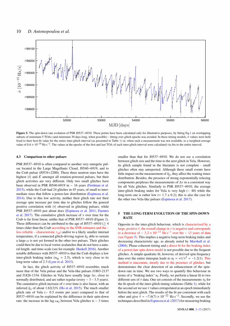
Finally, the history of the spin-down rate is presented in Figure5. As can be seen in this plot, the effect of glitches in the spin-down evolution is rather dramatic. A quasi-linear decay of | Ûν | isclearly seen after each glitch (or, in the case of the first glitch, oncethe exponential recovery no longer dominates), implying inter-glitchbraking indices well above 3; on the other hand, overall, there is a netincrease in the spin-down rate over the course of the observations.This, in turn, can be associated with a negative long-term “brakingindex”. We will discuss the physical interpretation of these resultsin the following.

4 GLITCH PROPERTIES AND INTERPRETATION

In the previous section we identified and parameterized, as con-sistently as possible, 45 glitches contained in the RXTE data ofPSR J0537−6910. Figure 3 presents these glitches in a ∆ Ûν − ∆νdiagram, together with detectability limits for recovering (∆ Ûν < 0)glitches derived according to Equation 2 in Espinoza et al. (2014).We use a value of 300 µs as the maximum between TOA error andthe RMS of the (inter-glitch) phase residuals, and two different ob-servation cadences of 10 and 30 days. The values for these threeparameters were chosen in order to obtain a very conservative esti-mate of the detection limits. As can be seen in figure 1, typically theTOA error and RMS are much smaller than 300 µs, and observa-tions are usually separated by no more than two weeks. This givesus confidence that our glitch sample is complete above, at least,∆ν ' 1 µHz. Most likely all glitches in the examined dataset thathad ∆ν & 0.3 µHz have been detected, unless they had an excep-tionally large ∆ Ûν and occurred in the few observing periods with

4 For the first glitch, the displayed size is the sum of the persisting anddecaying component.

0

100

200

300

400

500

600

700

2000 2002 2004 2006 2008 2010 2012Year

Cum

ulative Δν

(μH

z)

52000 53000 54000 55000 56000MJD

0

10

20

30

40

5

15

25 35 45

Δν (μ

Hz)

Figure 2. Glitches in PSR J0537−6910. Top panel: The cumulative increasein spin frequency over time due to the abrupt changes at glitches. The glitchactivity parameter (see Section 4.1) can be extracted by a linear fit in thisplot. Lower panel: The sizes and distribution of the 45 glitches in time.

TOA separation > 20 − 30 days. We will now examine the proper-ties of the glitch population of PSR J0537−6910, and discuss theirimplications in a simple superfluid glitch model framework.

4.1 The frequency changes

The spin-ups, ∆ν, span about two orders of magnitude. In otherpulsars with such a broad range of glitch sizes, a power-law providesa good description of the distribution (Melatos et al. 2008; Espinozaet al. 2014). In the case of PSR J0537−6910 however, glitch sizesappear to be normally distributed, with a mean ' 15.9 µHz andstandard deviation ' 10.8 µHz (probability 85% and 89% usingthe Cramer von Mises or K–S test respectively). The glitch “waitingtimes" ∆T are consistent with a Weibull distribution (Cramer vonMises probability 94%), with shape and scale parameters 1.74 and118.4 days respectively (with a mode of 72.5 days and mean 105.5days).

The regularity in glitch size and recurrence times (Figure 2)

MNRAS 000, 1–13 (2017)


0.01 0.1 1 10 100

1

10

100

1000 not measured > 0


0 10 20 30 40

0

50

100

150

200

250

300

Figure 3. The time interval to the next glitch versus the spin-up sizeof the preceding one. The dashed line goes through the origin (slope 6.44 days/µHz) and is the best fit to the data.

from !cr

). On the other hand, the size of a glitch does not correlateto the time since the last one, as could perhaps be expected if, forexample, bigger glitches were driven by a larger superfluid regionthat had time to reach its critical lag.

Let us assume that neutron vortices in the glitch-driving re-gion are strongly pinned (completely immobilised) whilst! < !

cr

.At the glitch, vortices catastrophically unpin, move (and possiblyre-pin) on a much shorter timescale compared to the inter-glitchevolution. Therefore, the spin-down rate for this superfluid compo-nent (hereafter denoted G) is zero, €

G

= 0, between glitches. Atthe same time, the crust and all stellar components tightly coupledto it - summing up to a moment of inertia I

c

- spin down at a rate€c

(t) = 2 €c

(t), where €c

(t) can be calculated from the inter-glitchtiming model. The rotational lag !

G

(t) = G

c

(t) after a glitchat epoch t

g

thus evolves as

!G

(t > tg

) !G

(tg

) =π

€c

(t)dt . (3)

Excess angular momentum in the component G builds at arate I

G

| €c

|, which should be compared to its transfer rate to theobserved component, I

c

A, where

A =1

Tobs

’

is the activity parameter. For this pulsar A is very well defineddue to the high glitch rate and regularity, as illustrated in Figure 2.A linear fit suggests that the moment of inertia of the componentG, I

G

, accounts for 0.873 ± 0.005% of the moment of inertiathat follows the spin-up, I

c

. Even if the latter comprises most ofthe stellar moment of inertia, I

c

Itot, and there is strong crustalentrainment, the inferred I

G

can be accommodated by the innercrust for a reasonable range of neutron star masses (Chamel 2013,see however Ho et al. 2015 for the possible core contribution).

The spread of glitch sizes could arise either from dierencesin the fractional moment of inertia participating in each glitch, orincomplete transfer of the excess angular momentum (the decreasein lag |!

G

| , !cr

), or both. Let us examine the second possibilityin more detail. If corotation between region G and the crust isrestored at a glitch (!

G

(tg

) = 0), Eq. 3 becomes !G

(t > tg

) =c

(tg

) c

(t). By extrapolating the inter-glitch timing solutions

to the epochs of consecutive glitches, we find that the maximumpossible lag that is built between them can vary even by an order ofmagnitude. This discrepancy, unlikely to be due to a large changeof !

cr

on such a short timescale, indicates that !G

does not alwaysdrop to zero at a glitch and the observed range of glitch sizes canbe explained by dierences in !

G

alone. We are thus justified toassume, for simplicity, that I

G

is the same for each glitch.Adopting I

G

/Ic

= 8.73 103, an estimate for a lower limitof the critical lag follows from the size

c

of the largest observedglitch. By angular momentum conservation, I

G

|G

| = Ic

c

,!

G

= Ic+IGIG

c

where !G

is the drop in !G

. For G

c

,|!

G

| must not be in excess of !cr

, thus

!cr

Ic

+ IG

IG

c

' 3 102 rad/s. (4)

The lag increase during the longest observed inter-glitch interval(between the first and second glitch) leads to a very similar minimumfor!

cr

of 3.1102 rad/s, but relies on the uncertain extrapolationof the inter-glitch timing solution to the glitch epochs.

If we were to relax our assumptions, the limits for the criticallag would change. For example, a partial coupling of region G( €

G

< 0) would reduce the inferred !cr

and require a realistictreatment of the superfluid’s dierential rotation. On the other hand,if the region where vortices are immobilised is not disconnectedfrom superfluid regions closer to the rotational axis that allow vortexcurrents, vortices could accumulate there and the real critical lagcould even be higher than our estimate.

4.2 The spin-down rate changes

A negative change of the spin-down €c

= 2 €, unresolved in time,accompanies the majority of glitches. The post-glitch € evolutionis well approximated by a linear increase (decreasing magnitude ofspin-down rate), untill the epoch of the next glitch. The only excep-tion to this nearly linear behaviour is the first (and largest) glitch, forwhich the inclusion of a short-term ( 20 days) exponential recov-ery in the timing model significantly improves the residuals. Theinter-glitch evolution is characterised by a positive ‹ of the order1020 Hz/s2, and large braking indices (n

ig

22 on average, seeTable 1).

The measurements of € are less accurate than those of ,hindering a robust statistical analysis. Using only those glitches (37out of 45) that have a clear detection of € < 0, the best-fit distri-bution is normal with mean ' 118.4 1015 Hz/s and standarddeviation' 44.41015 Hz/s (Cramer von Mises probability 94%).We do not observe a hard upper limit of | € | ' 1501015 Hz/s assuggested by Middleditch et al. (2006), but according to the abovedistribution the probability for | € | > 200 1015 Hz/s is indeedvery low.

The changes € for all glitches do not appear to correlatewith . Furthermore, we do not find evidence for the correlationbetween the time interval preceding a glitch and the change €which was reported by Middleditch et al.. We noted though that thesmallest glitches of our sample ( > 1 µHz) do not demonstrate thesame behaviour as the rest, that is, none of them has a clear negativechange in €. Instead, glitches 7, 27 and 41 have € consistent withbeing zero, and the timing solution for glitch 44 gave a positive € but with a large fractional error (0.85) thus potentially alsohad no eect on €. Assuming that these small spin-ups do not actto “reset" the clock for the spin-down rate changes, we calculated“waiting times" only between glitches with > 1 µHz (41 events).

MNRAS 000, 1–12 (2017)


0 10 20 30 40

0

50

100

150

200

250

300

Figure 3. The time interval to the next glitch versus the spin-up sizeof the preceding one. The dashed line goes through the origin (slope 6.44 days/µHz) and is the best fit to the data.

from !cr

). On the other hand, the size of a glitch does not correlateto the time since the last one, as could perhaps be expected if, forexample, bigger glitches were driven by a larger superfluid regionthat had time to reach its critical lag.

Let us assume that neutron vortices in the glitch-driving re-gion are strongly pinned (completely immobilised) whilst! < !

cr

.At the glitch, vortices catastrophically unpin, move (and possiblyre-pin) on a much shorter timescale compared to the inter-glitchevolution. Therefore, the spin-down rate for this superfluid compo-nent (hereafter denoted G) is zero, €

G

= 0, between glitches. Atthe same time, the crust and all stellar components tightly coupledto it - summing up to a moment of inertia I

c

- spin down at a rate€c

(t) = 2 €c

(t), where €c

(t) can be calculated from the inter-glitchtiming model. The rotational lag !

G

(t) = G

c

(t) after a glitchat epoch t

g

thus evolves as

!G

(t > tg

) !G

(tg

) =π

€c

(t)dt . (3)

Excess angular momentum in the component G builds at arate I

G

| €c

|, which should be compared to its transfer rate to theobserved component, I

c

A, where

A =1

Tobs

’

is the activity parameter. For this pulsar A is very well defineddue to the high glitch rate and regularity, as illustrated in Figure 2.A linear fit suggests that the moment of inertia of the componentG, I

G

, accounts for 0.873 ± 0.005% of the moment of inertiathat follows the spin-up, I

c

. Even if the latter comprises most ofthe stellar moment of inertia, I

c

Itot, and there is strong crustalentrainment, the inferred I

G

can be accommodated by the innercrust for a reasonable range of neutron star masses (Chamel 2013,see however Ho et al. 2015 for the possible core contribution).

The spread of glitch sizes could arise either from dierencesin the fractional moment of inertia participating in each glitch, orincomplete transfer of the excess angular momentum (the decreasein lag |!

G

| , !cr

), or both. Let us examine the second possibilityin more detail. If corotation between region G and the crust isrestored at a glitch (!

G

(tg

) = 0), Eq. 3 becomes !G

(t > tg

) =c

(tg

) c

(t). By extrapolating the inter-glitch timing solutions

to the epochs of consecutive glitches, we find that the maximumpossible lag that is built between them can vary even by an order ofmagnitude. This discrepancy, unlikely to be due to a large changeof !

cr

on such a short timescale, indicates that !G

does not alwaysdrop to zero at a glitch and the observed range of glitch sizes canbe explained by dierences in !

G

alone. We are thus justified toassume, for simplicity, that I

G

is the same for each glitch.Adopting I

G

/Ic

= 8.73 103, an estimate for a lower limitof the critical lag follows from the size

c

of the largest observedglitch. By angular momentum conservation, I

G

|G

| = Ic

c

,!

G

= Ic+IGIG

c

where !G

is the drop in !G

. For G

c

,|!

G

| must not be in excess of !cr

, thus

!cr

Ic

+ IG

IG

c

' 3 102 rad/s. (4)

The lag increase during the longest observed inter-glitch interval(between the first and second glitch) leads to a very similar minimumfor!

cr

of 3.1102 rad/s, but relies on the uncertain extrapolationof the inter-glitch timing solution to the glitch epochs.

If we were to relax our assumptions, the limits for the criticallag would change. For example, a partial coupling of region G( €

G

< 0) would reduce the inferred !cr

and require a realistictreatment of the superfluid’s dierential rotation. On the other hand,if the region where vortices are immobilised is not disconnectedfrom superfluid regions closer to the rotational axis that allow vortexcurrents, vortices could accumulate there and the real critical lagcould even be higher than our estimate.


A negative change of the spin-down €c

= 2 €, unresolved in time,accompanies the majority of glitches. The post-glitch € evolutionis well approximated by a linear increase (decreasing magnitude ofspin-down rate), untill the epoch of the next glitch. The only excep-tion to this nearly linear behaviour is the first (and largest) glitch, forwhich the inclusion of a short-term ( 20 days) exponential recov-ery in the timing model significantly improves the residuals. Theinter-glitch evolution is characterised by a positive ‹ of the order1020 Hz/s2, and large braking indices (n

ig

22 on average, seeTable 1).

The measurements of € are less accurate than those of ,hindering a robust statistical analysis. Using only those glitches (37out of 45) that have a clear detection of € < 0, the best-fit distri-bution is normal with mean ' 118.4 1015 Hz/s and standarddeviation' 44.41015 Hz/s (Cramer von Mises probability 94%).We do not observe a hard upper limit of | € | ' 1501015 Hz/s assuggested by Middleditch et al. (2006), but according to the abovedistribution the probability for | € | > 200 1015 Hz/s is indeedvery low.

The changes € for all glitches do not appear to correlatewith . Furthermore, we do not find evidence for the correlationbetween the time interval preceding a glitch and the change €which was reported by Middleditch et al.. We noted though that thesmallest glitches of our sample ( > 1 µHz) do not demonstrate thesame behaviour as the rest, that is, none of them has a clear negativechange in €. Instead, glitches 7, 27 and 41 have € consistent withbeing zero, and the timing solution for glitch 44 gave a positive € but with a large fractional error (0.85) thus potentially alsohad no eect on €. Assuming that these small spin-ups do not actto “reset" the clock for the spin-down rate changes, we calculated“waiting times" only between glitches with > 1 µHz (41 events).

MNRAS 000, 1–12 (2017)

|Δν| (μHz)

|Δν|

(10

-15 H

z s-1

)

·

300 μs

10 da

ys

30 da

ys

Figure 3. Conservative glitch detection limits and the changes in frequency,∆ν, and spin-down rate, |∆ Ûν |, for the 40 glitches with ∆ Ûν < 0 (blue dia-monds). Only the change ∆ν is shown for the 3 glitches with ∆ Ûν > 0 (blackcircles) and the two glitches for which ∆ Ûν was not fitted for (black crosses).The solid line represents the detection limit for phase residuals or TOAerror of 300µs, while the two dashed lines correspond to the limits due toTOA separation greater than 10 and 30 days. Glitches with (∆ν, ∆ Ûν < 0)above these lines would not have been identified in observations with suchrespective parameters.

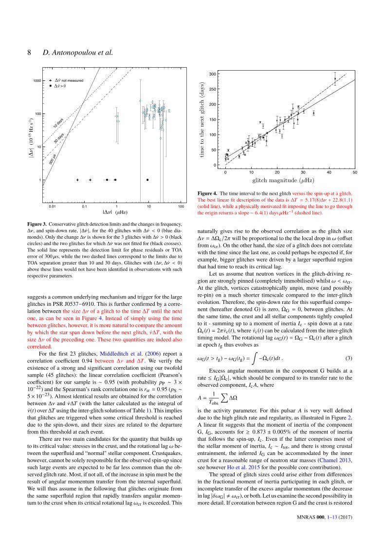
suggests a common underlying mechanism and trigger for the largeglitches in PSR J0537−6910. This is further confirmed by a corre-lation between the size ∆ν of a glitch to the time ∆T until the nextone, as can be seen in Figure 4. Instead of simply using the timebetween glitches, however, it is more natural to compare the amountby which the star span down before the next glitch, Ûν∆T , with thesize ∆ν of the preceding one. These two quantities are indeed alsocorrelated.

For the first 23 glitches, Middleditch et al. (2006) report acorrelation coefficient 0.94 between ∆ν and ∆T . We verify theexistence of a strong and significant correlation using our twofoldsample (45 glitches): the linear correlation coefficient (Pearson’scoefficient) for our sample is ∼ 0.95 (with probability pP ∼ 3 ×10−22) and the Spearman’s rank correlation one is rsr = 0.95 (pS ∼5× 10−23). Almost identical results are obtained for the correlationbetween ∆ν and Ûν∆T (with the latter calculated as the integral ofÛν(t) over∆T using the inter-glitch solutions of Table 1). This impliesthat glitches are triggered when some critical threshold is reacheddue to the spin-down, and their sizes are related to the departurefrom this threshold at each event.

There are two main candidates for the quantity that builds upto its critical value: stresses in the crust, and the rotational lag ω be-tween the superfluid and “normal" stellar component. Crustquakes,however, cannot be solely responsible for the observed spin-up sincesuch large events are expected to be far less common than the ob-served glitch rate. Most, if not all, of the increase in spin must be theresult of angular momentum transfer from the internal superfluid.We will thus assume in the following that glitches originate fromthe same superfluid region that rapidly transfers angular momen-tum to the crust when its critical rotational lagωcr is exceeded. This

0 10 20 30 40 50

0

50

100

150

200

250

300

timeto

thenextglitch

(days)

glitch

magn

itude(µHz)

1

time to the next glitch (days)

glitch magnitude (µHz)

1

Figure 4. The time interval to the next glitch versus the spin-up at a glitch.The best linear fit description of the data is ∆T = 5.17(8)∆ν + 22.8(1.1)(solid line), while a physically motivated fit imposing the line to go throughthe origin returns a slope ∼ 6.4(1) daysµHz−1 (dashed line).

naturally gives rise to the observed correlation as the glitch size∆ν = ∆Ωc/2π will be proportional to the the local drop in ω (offsetfrom ωcr). On the other hand, the size of a glitch does not correlatewith the time since the last one, as could perhaps be expected if, forexample, bigger glitches were driven by a larger superfluid regionthat had time to reach its critical lag.

Let us assume that neutron vortices in the glitch-driving re-gion are strongly pinned (completely immobilised) whilst ω < ωcr.At the glitch, vortices catastrophically unpin, move (and possiblyre-pin) on a much shorter timescale compared to the inter-glitchevolution. Therefore, the spin-down rate for this superfluid compo-nent (hereafter denoted G) is zero, ÛΩG = 0, between glitches. Atthe same time, the crust and all stellar components tightly coupledto it - summing up to a moment of inertia Ic - spin down at a rateÛΩc(t) = 2π Ûνc(t), where Ûνc(t) can be calculated from the inter-glitchtiming model. The rotational lag ωG(t) = ΩG −Ωc(t) after a glitchat epoch tg thus evolves as

ωG(t > tg) − ωG(tg) =∫− ÛΩc(t)dt . (3)

Excess angular momentum in the component G builds at arate ≤ IG | ÛΩc |, which should be compared to its transfer rate to theobserved component, Ic A, where

A =1

Tobs

∑∆Ω

is the activity parameter. For this pulsar A is very well defineddue to the high glitch rate and regularity, as illustrated in Figure 2.A linear fit suggests that the moment of inertia of the componentG, IG, accounts for ≥ 0.873 ± 0.005% of the moment of inertiathat follows the spin-up, Ic. Even if the latter comprises most ofthe stellar moment of inertia, Ic ∼ Itot, and there is strong crustalentrainment, the inferred IG can be accommodated by the innercrust for a reasonable range of neutron star masses (Chamel 2013,see however Ho et al. 2015 for the possible core contribution).

The spread of glitch sizes could arise either from differencesin the fractional moment of inertia participating in each glitch, orincomplete transfer of the excess angular momentum (the decreasein lag |δωG | , ωcr), or both. Let us examine the second possibility inmore detail. If corotation between region G and the crust is restored

MNRAS 000, 1–13 (2017)


at a glitch (ωG(tg) = 0), Eq. 3 becomesωG(t > tg) = Ωc(tg)−Ωc(t).By extrapolating the inter-glitch timing solutions to the epochs ofconsecutive glitches, we find that the maximum possible lag that isbuilt up can vary even by an order of magnitude. This discrepancy,unlikely to be due to a large change ofωcr on such a short timescale,indicates that ωG does not always drop to zero at a glitch and theobserved range of glitch sizes can be explained by differences inδωG alone. We are thus justified to assume, for simplicity, that IGis the same for each glitch.

Adopting IG/Ic = 8.73 × 10−3, an estimate for a lower limitof the critical lag follows from the size ∆Ωc of the largest observedglitch. By angular momentum conservation, IG |∆ΩG | = Ic∆Ωc,

δωG = −Ic + IG

IG∆Ωc

where δωG is the drop in ωG. For ΩG ≥ Ωc, |δωG | must not be inexcess of ωcr, thus

ωcr ≥Ic + IG

IG∆Ωc ' 3 × 10−2 rad s−1. (4)

The lag increase during the longest observed inter-glitch interval(between the first and second glitch) leads to a very similarminimumforωcr of 3.1×10−2 rad s−1, but relies on the uncertain extrapolationof the inter-glitch timing solution to the glitch epochs.

If we were to relax our assumptions, the limits for the criticallag would change. For example, a partial coupling of region G( ÛΩG < 0) would reduce the inferred ωcr and require a realistictreatment of the superfluid’s differential rotation. On the other hand,if the region where vortices are immobilised is not disconnectedfrom superfluid regions closer to the rotational axis that allow vortexcurrents, vortices could accumulate there and the real critical lagcould even be higher than our estimate.


A negative change of the spin-down ÛΩc = 2π Ûν, unresolved in time,accompanies the majority of glitches. The post-glitch Ûν evolutionis well approximated by a linear increase (decreasing magnitude ofspin-down rate), until the epoch of the next glitch. The only excep-tion to this nearly linear behaviour is the first (and largest) glitch, forwhich the inclusion of a short-term (∼ 20 days) exponential recov-ery in the timing model significantly improves the residuals. Theinter-glitch evolution is characterised by a positive Üν of the order10−20 Hz s−2, and large braking indices (nig ∼ 22 on average, seeTable 1).

The measurements of ∆ Ûν are less accurate than those of ∆ν,hindering a robust statistical analysis. Using only those glitches(37 out of 45) that have a clear detection of ∆ Ûν < 0, the best-fit distribution is normal with mean ' −118.4 × 10−15 Hz s−1

and standard deviation ' 44.4 × 10−15 Hz s−1 (Cramer von Misesprobability 94%). We do not observe a hard upper limit of |∆ Ûν | '150 × 10−15 Hz s−1 as suggested by Middleditch et al. (2006), butaccording to the above distribution the probability for |∆ Ûν | > 200×10−15 Hz s−1 is indeed very low.

The changes ∆ Ûν for all glitches do not appear to correlatewith ∆ν. Furthermore, we do not find evidence for the correlationbetween the time interval preceding a glitch and the change ∆ Ûνwhich was reported by Middleditch et al.. We noted though that thesmallest glitches of our sample (∆ν < 1 µHz) do not demonstrate thesame behaviour as the rest, that is, none of them has a clear negativechange in Ûν. Instead, glitches 7, 27 and 41 have ∆ Ûν consistent withbeing zero, and the timing solution for glitch 44 gave a positive

∆ Ûν but with a large fractional error (0.85) thus potentially alsohad no effect on Ûν. Assuming that these small spin-ups do not actto “reset" the clock for the spin-down rate changes5, we calculated“waiting times" only between glitches with∆ν > 1 µHz (41 events).Then a somewhat weak but significant correlation (rsr = 0.57,pS ∼ 2 × 10−4) emerges.

In the simplest case, the neutron star comprises of threecomponents, Ic, IG and In such that the total moment of in-ertia is Itot = Ic + IG + In and the total angular momentumLtot = IcΩc + IGΩG + InΩn. The component In consists of anysuperfluid region that is loosely coupled to Ic: if vortices are notimmobilised due to pinning (as in the region G), their outwards mo-tion allows for a non-zero | ÛΩn | ≤ | ÛΩc |, with the equality definingan “equilibrium" lag ωs. Since ÛΩG(t , tg) = 0, IG is decoupledbefore and after the glitch and does not contribute to the observedinter-glitch spin-down, which is described by

Ic ÛΩc + In ÛΩn = Next . (5)

For standard dipole braking, the external torque is

Next = −B2⊥R6

?

6c3 Ω3c, (6)

where B⊥ = Bp sinα, Bp the polar dipole magnetic field compo-nent, α its angle to the rotational axis, and R? the stellar radius. Atany given moment, the observed magnitude of the spin-down rateis therefore bound between a maximum of | ÛΩc |max = |Next |/Ic, anda minimum | ÛΩc |min = |Next |/(Ic + In) when the “equilibrium" lagis reached. When a glitch occurs, any loosely coupled superfluidregion will be driven out (or further away) of its equilibrium lag,which results in the observed abrupt increase in spin-down rate.

The change in ÛΩc provides a lower limit for the component Inthat can decouple at the glitch. Assuming a torque as in Equation6 and that on short timescales it changes only due to the varyingΩc(t), then

InIc≥ÛΩ

postc − ÛΩ

prec

ÛΩprec

, (7)

where ÛΩprec is the spin-down rate immediately before the glitch and

ÛΩpostc is at time t > tg such thatΩ

postc < Ω

prec . We evaluate this using

the epochs of the TOAs surrounding each glitch as tpre and tpost.Although an earlier tpost would lead to tighter constraints, we preferto avoid a less accurate extrapolation of the timing model closer tothe (unknown) glitch epoch. The obtained constraint isInIc≥ 1.4 × 10−3 .

While observed ∆ ÛΩc/ ÛΩc is usually 10−4 − 10−3, immediatelyafter the glitch the decoupled fraction of the superfluid can bemuch higher, as has been inferred for other pulsars (Lyne et al.2000; Dodson et al. 2002). Usually such large changes recoverquickly, often in an exponential manner with various characteristictimescales, from few hours to several days. If present, such a strongrelaxation would have been easily missed for PSR J0537−6910: itsvery fast rotation compared to other pulsars shortens considerablythe re-coupling timescales, while the monitoring cadence was notvery high. Both glitch parameters∆Ω and∆ ÛΩ should then be viewedas lower limits of their counterparts at the glitch epoch.

5 For example, this could be the case if the inferred spin-up was gradual,rather than abrupt as in larger glitches. Excluding these small irregularitiesfrom the glitch sample has little impact on the ∆ν analysis and does not alterthe main conclusions.

MNRAS 000, 1–13 (2017)


52000 53000 54000 55000 56000

-199600

-199500

-199400

-199300

-199200

-199100

MJD [days]

[10

15Hz/s]

Figure 5. The spin-down rate evolution of PSR J0537−6910. These points have been calculated only for illustrative purposes, by fitting Eq.1 on overlappingsubsets of minimum 5 TOAs (and minimum 30 days long, when possible) – fitting over glitch epochs was avoided. In these timing models, Üν values were heldfixed to their best-fit value for the entire inter-glitch interval (as presented in Table 1) or, when such a measurement was not available, to a weighted averagevalue of 0.6 × 10−20 Hz s−2. The values at the epochs of the first and last TOA of each inter-glitch interval were calculated via fits to the entire interval.

4.3 Comparison to other pulsars

PSR J0537−6910 is often compared to another very energetic pul-sar located in the Large Magellanic Cloud, J0540−6919, and tothe Crab pulsar (J0534+2200). These three neutron stars have thehighest | Ûν | and ÛE amongst all rotation-powered pulsars, but theirglitch activities are very different. Only two small glitches havebeen observed in PSR J0540-6919 in ∼ 16 years (Ferdman et al.2015), while the Crab had 24 glitches in 45 years, of small to inter-mediate sizes that follow a power-law distribution (Espinoza et al.2014). Due to this low activity, neither their glitch rate nor theiraverage spin increase per time due to glitches follow the generalpositive correlation with | Ûν | observed in glitching pulsars, whilePSR J0537−6910 just about does (Espinoza et al. 2011; Fuenteset al. 2017). The cumulative glitch increase of ν over time for theCrab is far from linear, unlike that of PSR J0537−6910 (Figure 2).These differences can be attributed to the age of J0537−6910 (& 4times older than the Crab according to the SNR estimates and the –less reliable – characteristic τsd) and/or to a likely smaller internaltemperature, if a connected glitch-driving region IG able to sustaina large ω is not yet formed in the other two pulsars. Their glitchescould then be due to local vortex avalanches that do not have a natu-ral length- and time-scale (see for example Haskell 2016). Anothernotable difference with J0537−6910 is that the Crab displays a lowinter-glitch braking index (nig ' 2.5), which is very close to itslong-term value of 2.3 (Lyne et al. 2015).

In fact, the glitch activity of J0537−6910 resembles muchmore that of the Vela pulsar and the Vela-like pulsars J1803-2137and J1826-1334. Glitches in Vela have usually large ∆ν, close tonormally distributed, and are rather regular (every ∼ 3− 3.5 years).The cumulative glitch increase of ν over time is also linear, with aninferred IG of about 1.62(3)% (Ho et al. 2015). The much smallerglitch rate of Vela (∼ 0.5 events per year) compared to that ofJ0537−6910 can be explained by the difference in their spin-downrate: the increase in the lag ωG between Vela glitches is ∼ 3 times

smaller than that for J0537−6910. We do not see a correlationbetween glitch size and the time to the next glitch in Vela. However,its glitch sample found in the literature is not complete - smallglitches often stay unreported. Although these small events havelittle impact on the measurement of IG, they affect the waiting timesdistribution. Besides, the presence of strong exponentially relaxingcomponents perplexes the measurements of ∆ν in a consistent wayfor all Vela glitches. Similarly to PSR J0537−6910, the averageinter-glitch braking index for Vela is very high (∼ 40) while thelong-term one is rather low (= 1.7 ± 0.2); this is also the case forthe other two Vela-like pulsars (Espinoza et al. 2017).

5 THE LONG-TERM EVOLUTION OF THE SPIN-DOWNRATE

Opposite to the inter-glitch behaviour, which is characterised by alarge, positive Üν, the overall change in Ûν is negative and correspondsto a decrease of ∼ 3.2 × 10−13 Hz s−1 over the ∼ 13 years of data(see Figure 5). This implies a negative long-term braking index anddecreasing characteristic age, as already noted by Marshall et al.(2004). Phase-coherent timing and a direct fit for the braking indexof a power-law spin-down model is not possible due to the frequentglitches. A simple quadratic fit, however, of derived spin frequencydata over the entire timespan leads to nl = ν Üν/ Ûν

2 = −1.2(1). Thismethod is inaccurate, mostly due to the presence of glitches, butdemonstrates the clear detection of an enhancement of the spin-down rate in time. We use two ways to quantify this behaviour interms of a “braking index" nl. Firstly, we perform a linear fit to twodifferent sets of Ûν data. One set consists of the measurements Ûν0 forthe fit epoch of the inter-glitch timing solutions (Table 1), while forthe second set we use Ûν values extrapolated at an epoch immediatelybefore the next glitch. The results of the fit are consistent with eachother and give Üν = −7.6(7) × 10−22 Hz s−2. Secondly, we use thetechniques described inEspinoza et al. (2017) formeasuring braking

MNRAS 000, 1–13 (2017)


indices in pulsars with large and regular glitches. The method isbased on constructing a Ûν-template which is used to calculate therelative Ûν shifts of each inter-glitch interval. Together with the glitchepochs, these define a set of ( Ûν, t) points that follow a straight line(linear correlation coefficient 0.976) fromwhich the long-term Üν canbe inferred. For PSR J0537−6910, we use the 39 largest glitchesand a 160-days long template constructed from their post-glitchcurves. In line with our previous estimates, we obtain a long-termÜν = −7.7(3) × 10−22 Hz s−2 and a corresponding braking indexnl = −1.22(4).

Identifying the possible mechanism behind the unusual in-crease in spin-down rate depends on whether this change is con-tinuous, or happens in discrete steps (for example in relation to theglitches), or a combination of both. Unfortunately we were not ableto confidently discriminate between these options from the data athand. We outline some possibilities below and give quantitative es-timates under the assumption that - for the time interval of interest -the actual braking index n is constant. To obtain numerical results weoften assume an underlying power-law braking with n = 3, howevervarious mechanisms contribute to the evolution of Ûν, some of whichmight not even have a power-law form (one such example couldbe the internal torque due to the superfluid dynamics). Moreover,there is a wide range of reported long-term braking indices for otheryoung pulsars, the majority of which is under 3 (see for exampleLyne et al. (2015); Espinoza et al. (2017) and references therein).Although some of the same physical processes might be responsiblefor all observed low (< 3) braking indices, PSR J0537−6910 is theonly rotationally-powered pulsar with a net increase in | Ûν | over somany years.

A decreasing effective moment of inertia Ic could result inbraking indices less than three. Ho & Andersson (2012) modelled adecreasing Ic as the result of an ongoing formation of new superfluidregions as they cool below the critical temperature for superfluidity.An increasing fraction of the interior then decouples, leaving asmaller moment of inertia to respond to the (nearly constant) spin-down torque (which we take here as the standard dipole braking,Eq. 6). If the two fluids are completely decoupled ( ÛΩs = 0) and(Ωs −Ωc)/Ωc 1 then

nl ' 3 − 2ÛIIΩcÛΩc⇒ ÛI ' 2 × 1041

(I

1045g cm2

)g cm2 yr−1

is required to explain the observed braking index of−1.2. One of themain challenges of this model is to accommodate the low brakingindex of the - relatively old and cool - Vela pulsar consistently withthe constraints for the (de)coupled superfluid moment of inertiathat come from glitch observations6. A similar, also short-livedcompared to τsd, effect of decreasing Ic will arise if the coupling insome, already superfluid, regions becomes weaker; this can be donealso in discrete steps, for example if small crustquakes leave thenuclei lattice deformed in such a way that vortex pinning becomesstronger (Alpar et al. 1996).

Accumulated offsets∆ Ûν < 0, due to the frequent glitcheswhichdecouple the internal superfluid, could mimic a negative long-termÜν. After all, the very high nig up to the time of a following glitchmeans that the recoupling of the superfluid still carries on. Thismechanism requires the progressive decoupling of a superfluid ef-fective moment of inertia Is additional to In that does not recoupleon observable timescales. If the persisting offsets arose only from

6 ÛΩs = 0 cannot hold in the bulk of the star if the post-glitch relaxation isof superfluid origin.

parts of the In component that did not have the time to recover till thenext glitch, then | ÛΩc |min would change but | ÛΩc |max would remainlimited at |Next |/Ic. Instead, as clearly seen in Figure 5, | ÛΩc |max

also follows an increasing trend; moreover, measurements of ∆ Ûν/ Ûνshow no convincing evidence for a decreasing In/Ic over time. Inthis scenario, the Is that needs to have decoupled during the RXTEobservations needs to be of the order 10−3I.

It is worth noting that glitches in at least two pulsars left long-lasting decreases in their braking indices (Livingstone et al. 2011;Antonopoulou et al. 2015), mainly due to a drop in Üν after the initialpost-glitch recovery stages were over. A period of higher glitchactivity of the Crab pulsar is also associated with a decrease of itsbraking index, even after some persisting glitch offsets have beencorrected for (Lyne et al. 2015), and 9 out of the 12 pulsars witha measured long-term n < 3 have known glitches (Espinoza et al.2017, and references therein). It is perhaps then not surprising thatPSR J0537−6910, with its unprecedented high rate of large glitches,has the smallest braking index of all.

Another possibility is an increasing torque as a result of mag-netic field evolution. We consider a spin-down that is governed by

ÛΩc = − f (?)B2?Ω

nc

which makes the assumption that the superfluid is either completelydecoupled ( ÛΩs = 0) or in equilibrium with the normal component( ÛΩs = ÛΩc). Here, f (?) is a function of stellar parameters that willbe taken constant in time, B? = g(α)Bp with g(α) a trigonometricfunction of α, and n is the real, underlying braking index. Allowingfor a changing B? means that the observed braking index will be

nl = n + 2ΩcÛΩc

ÛB?B?

(8)

which implies, for nl = −1.2, n = 3 and constant g(α):

ÛBp ' 6.8(

| Ûνc |

2 × 10−10Hz s−1

) ( ν

62Hz

)−1(

Bp

1012G

)G s−1 .

It has been suggested that such a ÛBp could be due to field reemer-gence from the crust following an initial mass accretion (see forexample Muslimov & Page 1996; Pons et al. 2012), although itis unclear whether PSR J0537−6910 could have accreted enoughmaterial for the required field burial because it has a large inferredkick velocity (Ng & Romani 2007, but see also Güneydaş & Ekşi2013). An amplification of the dipole component due to Hall driftat early timescales has been also proposed (Gourgouliatos & Cum-ming 2015), but requires an exceptionally strong magnetic field inthe crust.

Alternatively, ÛB? can be due to an increasing misalignment ofthe magnetic and rotational axes, while the magnetic field strengthremains almost constant ( ÛBp = 0). Middleditch et al. (2006) ex-plored this idea in detail, taking α to be a linear function of timeand the intrinsic braking index n to be less than 3, to track thebirth values of α and ν. Discrete shifts ∆α in the inclination anglehave been invoked to explain persisting changes of the rotationalparameters after glitches, seen in several pulsars (Link et al. 1992;Link & Epstein 1997; Akbal et al. 2015). In the case of the Crabpulsar, however, the sum of possible glitch-associated ∆α over thetotal observing time does not suffice to explain the deviation of itsbraking index from 3 (Lyne et al. 2015), nor the recently reportedevidence for increasing phase separation between its main pulseand interpulse (Lyne et al. 2013) which suggests a non-zero inter-glitch Ûα. From Equation 8, for g(α) = sinα(t), Bp = const we get

MNRAS 000, 1–13 (2017)


cotα Ûα = (nl − n) Ûν/(2ν) or, for n = 3 and nl = −1.2:

Ûα

tanα= 6.8 × 10−12

(| Ûν |

2 × 10−10Hz s−1

) ( ν

62Hz

)−1rad s−1 . (9)

For a moderate α = 30 we get Ûα ' 0.7 degrees per century,remarkably close to the slow migration rate inferred for the Crabpulsar (Lyne et al. 2013).

6 SUMMARY AND CONCLUSIONS

We analysed all RXTE observations of the pulsar J0537−6910 withthe aim of reconstructing its rotational history and studying itsglitching activity. Twenty-one new glitches were identified, raisingtheir total number for this pulsar at 45 in nearly 13 years. Mostspin-ups are large and follow a broad Gaussian distribution withmean ∆ν ∼ 16 µHz. The first glitch in the data remains the largestand the only one for which some exponential decay of the spin-upis seen, on a characteristic timescale of ∼ 20 days. The rest wereadequately described by a model with step-like changes in the spinν, spin-down Ûν and sometimes Üν. The mean waiting time betweenglitches is 105.5 days and is strongly correlated to the size ∆ν ofthe preceding glitch. This fact can be used to predict the epoch ofthe subsequent spin-up.

Almost all glitches display an abrupt spin-down rate change,∆ Ûν < 0, with mean ∆ Ûν ∼ −120 × 10−12 Hz s−1. A correlation be-tween the waiting time and the size |∆ Ûν | of the following glitch,with a saturation at |∆ Ûν | ' 150× 10−12 Hz s−1 was noticed by Mid-dleditch et al. (2006). Such a finding would provide extra supportfor superfluid models of post-glitch relaxation but unfortunately itsconcrete confirmation was not possible using our results.

In a simple 3-component model of a neutron star, the observedglitch phenomenology can be explained as follows: A part of the su-perfluid, bearing less than 0.8% of the total moment of inertia, doesnot spin down at all in between glitches. Once its rotational veloc-ity exceeds that of the crust by & 0.03 rad s−1, it rapidly transferssome angular momentum to the non-superfluid (normal) compo-nent, causing a glitch. The rest of the superfluid follows the spin-upof the normal component on timescales that depend on couplingstrength between the two; an effective& 0.15% of the total momentof inertia remains decoupled on long enough timescales so that theobserved spin-down rate is higher post-glitch. The slow recouplingof this component is most likely responsible for the large inter-glitchbraking indices (nig ∼ 22).

Over the time span of the observations, the spin-down rateincreased by ∼ 0.15%, equivalent to a well-defined negative long-term Üν = −7.5(3) × 10−22 Hz s−2, unlike what is seen in any otheryoung pulsars. The inferred braking index for this behaviour is nl =−1.22(4) and could be attributed to the progressive decoupling of asuperfluid component (of ∼ 10−3 fractional moment of inertia), oran increasing external spin-down torque, e.g. as the pulsar becomesmore of an orthogonal rotator. The pulsar’s evolutionary path on theP − ÛP diagram points in the direction of the Crab pulsar (Espinozaet al. 2017). Clearly though, the duration of the phase with this lowbraking index cannot be very long compared to τsd . Although wewere unable to resolve a significant time variation of nl, it is notimpossible –albeit optimistic– to imagine that a measurable changecould be revealed in the coming years, given a good observationalcoverage.

PSR J0537−6910 has the highest spin frequency and spin-down luminosity of all known rotational-powered pulsars and aremarkable rotational evolution, vastly dominated by large glitches.

The high glitch rate of ∼ 3.5 per year and the predictability of thetime for a next glitch, given a firm measurement of the preced-ing one, makes this pulsar an ideal target for close observations ofa glitch’s rise, early recovery and possible emission changes withmissions like NICER, which are crucial for the advances of our the-oretical understanding of the phenomenon. Furthermore, long-termmonitoring might shed light to the mechanism behind the excep-tional negative long-term braking index observed for this pulsar.

ACKNOWLEDGMENTS

D.A. acknowledges support from the Polish National Science Cen-tre (SONATA BIS 2015/18/E/ST9/00577, P.I.: B. Haskell) andthe research networking programme NewCompStar (COST ActionMP1304). C.M.E. acknowledges support from FONDECYT Regu-lar Project 1171421.

REFERENCES

Akbal O., Gügercinoğlu E., Şaşmaz Muş S., Alpar M. A., 2015, MNRAS,449, 933

Alpar M. A., Baykal A., 2006, MNRAS, 372, 489Alpar M. A., Chau H. F., Cheng K. S., Pines D., 1996, ApJ, 459, 706Anderson P. W., Itoh N., 1975, Nature, 256, 25Antonopoulou D., Weltevrede P., Espinoza C. M., Watts A. L., Johnston S.,

Shannon R. M., Kerr M., 2015, MNRAS, 447, 3924Chamel N., 2013, Phys. Rev. Lett., 110, 011101Chu Y.-H., Kennicutt Jr. R. C., Schommer R. A., Laff J., 1992, AJ, 103,

1545Cognard I., Backer D. C., 2004, ApJ, 612, L125Crawford F., McLaughlin M., Johnston S., Romani R., Sorrelgreen E., 2005,

Advances in Space Research, 35, 1181Dodson R. G., McCulloch P. M., Lewis D. R., 2002, ApJ, 564, L85Espinoza C. M., Lyne A. G., Stappers B. W., Kramer M., 2011, MNRAS,

414, 1679Espinoza C. M., Antonopoulou D., Stappers B. W., Watts A., Lyne A. G.,

2014, MNRAS, 440, 2755Espinoza C. M., Lyne A. G., Stappers B. W., 2017, MNRAS, 466, 147Ferdman R. D., Archibald R. F., Kaspi V. M., 2015, ApJ, 812, 95Fuentes J. R., Espinoza C. M., Reisenegger A., 2017, Submitted to A&AGourgouliatos K. N., Cumming A., 2015, MNRAS, 446, 1121Güneydaş A., Ekşi K. Y., 2013, MNRAS, 430, L59Haskell B., 2016, MNRAS, 461, L77Haskell B., Melatos A., 2015, International Journal of Modern Physics D,

24, 1530008Ho W. C. G., Andersson N., 2012, Nature Physics, 8, 787Ho W. C. G., Espinoza C. M., Antonopoulou D., Andersson N., 2015,

Science Advances, 1, e1500578Hobbs G. B., Edwards R. T., Manchester R. N., 2006, MNRAS, 369, 655Kuiper L., Hermsen W., 2009, A&A, 501, 1031Kuiper L., Hermsen W., 2015, MNRAS, 449, 3827Link B., Epstein R. I., 1997, ApJ, 478, L91Link B., Epstein R. I., Baym G., 1992, ApJ, 390, L21LivingstoneM. A., Ng C.-Y., Kaspi V. M., Gavriil F. P., Gotthelf E. V., 2011,

ApJ, 730, 66Lyne A. G., Shemar S. L., Smith F. G., 2000, MNRAS, 315, 534Lyne A., Graham-Smith F., Weltevrede P., Jordan C., Stappers B., Bassa C.,

Kramer M., 2013, Science, 342, 598Lyne A. G., Jordan C. A., Graham-Smith F., Espinoza C.M., Stappers B.W.,

Weltevrede P., 2015, MNRAS, 446, 857Marshall F. E., Gotthelf E. V., Zhang W., Middleditch J., Wang Q. D., 1998,

ApJ, 499, L179Marshall F. E., Gotthelf E. V., Middleditch J., Wang Q. D., Zhang W., 2004,

Nature, 603, 682

MNRAS 000, 1–13 (2017)

http://dx.doi.org/10.1093/mnras/stv322

http://adsabs.harvard.edu/abs/2015MNRAS.449..933A

http://dx.doi.org/10.1111/j.1365-2966.2006.10893.x

http://adsabs.harvard.edu/abs/2006MNRAS.372..489A

http://dx.doi.org/10.1086/176935

http://adsabs.harvard.edu/abs/1996ApJ...459..706A

http://dx.doi.org/10.1038/256025a0

http://adsabs.harvard.edu/abs/1975Natur.256...25A

http://dx.doi.org/10.1093/mnras/stu2710

http://adsabs.harvard.edu/abs/2015MNRAS.447.3924A

http://dx.doi.org/10.1103/PhysRevLett.110.011101

http://adsabs.harvard.edu/abs/2013PhRvL.110a1101C

http://dx.doi.org/10.1086/116167

http://adsabs.harvard.edu/abs/1992AJ....103.1545C

http://adsabs.harvard.edu/abs/1992AJ....103.1545C

http://dx.doi.org/10.1086/424692

http://adsabs.harvard.edu/abs/2004ApJ...612L.125C

http://dx.doi.org/10.1016/j.asr.2005.03.074

http://adsabs.harvard.edu/abs/2005AdSpR..35.1181C

http://dx.doi.org/10.1086/339068

http://adsabs.harvard.edu/abs/2002ApJ...564L..85D

http://dx.doi.org/10.1111/j.1365-2966.2011.18503.x

http://adsabs.harvard.edu/abs/2011MNRAS.414.1679E


http://adsabs.harvard.edu/abs/2014MNRAS.440.2755E

http://dx.doi.org/10.1093/mnras/stw3081

http://adsabs.harvard.edu/abs/2017MNRAS.466..147E

http://dx.doi.org/10.1088/0004-637X/812/2/95

http://adsabs.harvard.edu/abs/2015ApJ...812...95F


http://adsabs.harvard.edu/abs/2015MNRAS.446.1121G

http://dx.doi.org/10.1093/mnrasl/sls050

http://adsabs.harvard.edu/abs/2013MNRAS.430L..59G

http://dx.doi.org/10.1093/mnrasl/slw103

http://adsabs.harvard.edu/abs/2016MNRAS.461L..77H

http://dx.doi.org/10.1142/S0218271815300086

http://adsabs.harvard.edu/abs/2015IJMPD..2430008H

http://dx.doi.org/10.1038/nphys2424

http://adsabs.harvard.edu/abs/2012NatPh...8..787H

http://dx.doi.org/10.1126/sciadv.1500578

http://dx.doi.org/10.1111/j.1365-2966.2006.10302.x

http://adsabs.harvard.edu/abs/2006MNRAS.369..655H

http://dx.doi.org/10.1051/0004-6361/200811580

http://adsabs.harvard.edu/abs/2009A%26A...501.1031K

http://dx.doi.org/10.1093/mnras/stv426

http://adsabs.harvard.edu/abs/2015MNRAS.449.3827K

http://dx.doi.org/10.1086/310549

http://adsabs.harvard.edu/abs/1997ApJ...478L..91L

http://dx.doi.org/10.1086/186362

http://adsabs.harvard.edu/abs/1992ApJ...390L..21L

http://dx.doi.org/10.1088/0004-637X/730/2/66

http://adsabs.harvard.edu/abs/2011ApJ...730...66L

http://dx.doi.org/10.1046/j.1365-8711.2000.03415.x

http://adsabs.harvard.edu/abs/2000MNRAS.315..534L

http://dx.doi.org/10.1126/science.1243254

http://adsabs.harvard.edu/abs/2013Sci...342..598L


http://adsabs.harvard.edu/abs/2015MNRAS.446..857L

http://dx.doi.org/10.1086/311381

http://adsabs.harvard.edu/abs/1998ApJ...499L.179M

http://dx.doi.org/10.1086/381567

http://adsabs.harvard.edu/abs/2004ApJ...603..682M


McKee J. W., et al., 2016, MNRAS, 461, 2809Melatos A., Peralta C., Wyithe J. S. B., 2008, ApJ, 672, 1103Middleditch J., Marshall F. E., Wang Q. D., Gotthelf E. V., Zhang W., 2006,

ApJ, 652, 1531Muslimov A., Page D., 1996, ApJ, 458, 347Ng C.-Y., Romani R. W., 2007, ApJ, 660, 1357Pons J. A., Viganò D., Geppert U., 2012, A&A, 547, A9Wang Q. D., Gotthelf E. V., 1998, ApJ, 494, 623Yu M., et al., 2013, MNRAS, 429, 688

MNRAS 000, 1–13 (2017)

http://dx.doi.org/10.1093/mnras/stw1442

http://adsabs.harvard.edu/abs/2016MNRAS.461.2809M

http://dx.doi.org/10.1086/523349

http://dx.doi.org/10.1086/508736

http://dx.doi.org/10.1086/176817

http://adsabs.harvard.edu/abs/1996ApJ...458..347M

http://dx.doi.org/10.1086/513597

http://adsabs.harvard.edu/abs/2007ApJ...660.1357N

http://dx.doi.org/10.1051/0004-6361/201220091

http://adsabs.harvard.edu/abs/2012A%26A...547A...9P

http://dx.doi.org/10.1086/305214

http://adsabs.harvard.edu/abs/1998ApJ...494..623W

http://dx.doi.org/10.1093/mnras/sts366

http://adsabs.harvard.edu/abs/2013MNRAS.429..688Y

pulsar spin-down: the glitch-dominated rotation of psr ... · pulsar spin-down: the...

Documents