pump fault detection and diagnosis (fdd) based on electrical … · pump fault detection and...

2.141 Term Project

Pump Fault Detection and Diagnosis (FDD) Based on Electrical Startup Transient

2002.12.12 Peter Armstrong

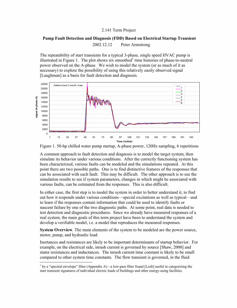
The repeatability of start transients for a typical 3-phase, single speed HVAC pump is

illustrated in Figure 1. The plot shows six smoothed1 time histories of phase-to-neutral

power observed on the A-phase. We wish to model the system (or as much of it as

necessary) to explore the possibility of using this relatively easily observed signal

[Laughman] as a basis for fault detection and diagnosis.

Figure 1. 50-hp chilled water pump startup, A-phase power, 120Hz sampling, 6 repetitions

A common approach to fault detection and diagnosis is to model the target system, then

simulate its behavior under various conditions. After the correctly functioning system has

been characterized, various faults can be modeled and the simulations repeated. At this

point there are two possible paths. One is to find distinctive features of the responses that

can be associated with each fault. This may be difficult. The other approach is to use the

simulation results to see if system parameters, changes in which might be associated with

various faults, can be estimated from the responses. This is also difficult.

In either case, the first step is to model the system in order to better understand it, to find

out how it responds under various conditions—special excitations as well as typical—and

to learn if the responses contain information that could be used to identify faults or

nascent failure by one of the two diagnostic paths. At some point, real data is needed to

test detection and diagnostic procedures. Since we already have measured responses of a

real system, the main goals of this term project have been to understand the system and

develop a verifiable model, i.e. a model that reproduces the measured responses.

System Overview. The main elements of the system to be modeled are the power source,

motor, pump, and hydraulic load.

Inertances and resistances are likely to be important determinants of startup behavior. For

example, on the electrical side, inrush current is governed by source [Shaw, 2000] and

stator resistances and inductances. The inrush current time constant is likely to be small

compared to other system time constants. The flow transient is governed, in the fluid

1 by a “spectral envelope” filter (Appendix A)—a low-pass filter found [Leeb] useful in categorizing the

start transient signatures of individual electric loads of buildings and other energy-using facilities.

Children's Court 17 June P4, 6 reps

0

2000

4000

6000

8000

10000

12000

14000

16000

18000

20000

22000

1 13 25 37 49 61 73 85 97 109 121 133 145 157 169 181 193

Time (1s/tick)

sig

nal (A

-ph

ase A

)

1

2

3

4

5

6

Armstrong 2/29

domain, by inertances and resistances in the piping circuit; it may, depending on coupling

and relative time scales, be significantly affected by motor and pump rotor inertances.

The non-linear natures of motor, pump, and load static performance are, of course, very

basic to the process because the entire range of operation is traversed during startup.

Ringing, evident on the tail in Figure 12, could stem from compliances in the motor field,

in mechanical coupling of motor to pump, or in the hydraulic circuit3. In the latter case,

compliances could be near to or remote from the pump—or distributed over the circuit.

Model 1. We can represent the motor, pump, and load by their non-linear static behaviors.

The source/nature of ringing can then be explored by inserting plausible compliances,

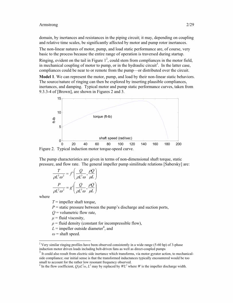
inertances, and damping. Typical motor and pump static performance curves, taken from

9.3.3-4 of [Brown], are shown in Figures 2 and 3.

Figure 2. Typical induction motor torque-speed curve.

The pump characteristics are given in terms of non-dimensional shaft torque, static

pressure, and flow rate. The general impeller pump similitude relations [Sabersky] are:

L

Q

L

Qg

L

P

L

Q

L

Qf

L

T

,'

,'

322

325

where

T = impeller shaft torque,

P = static pressure between the pump’s discharge and suction ports,

Q = volumetric flow rate,

µ = fluid viscosity,

= fluid density (constant for incompressible flow),

L = impeller outside diameter4, and

= shaft speed.

2 Very similar ringing profiles have been observed consistently in a wide range (5-60 hp) of 3-phase

induction motor driven loads including belt-driven fans as well as direct-coupled pumps 3 It could also result from electric side inertance which transforms, via motor gyrator action, to mechanical-

side compliance; our initial sense is that the transformed inductances typically encountered would be too

small to account for the rather low resonant frequency observed.4 In the flow coefficient, Q/ L3 , L3 may by replaced by WL2 where W is the impeller discharge width.

0 20 40 60 80 100 120 140 160 180 2000

5

10

15

ft-lb torque (ft-lb)

shaft speed (rad/sec)

Armstrong 3/29

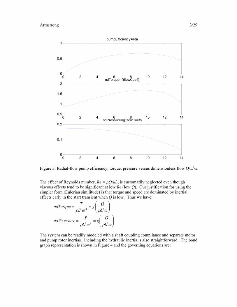
Figure 3. Radial-flow pump efficiency, torque, pressure versus dimensionless flow Q/L3

.

The effect of Reynolds number, Re = Q/µL, is customarily neglected even though

viscous effects tend to be significant at low Re (low Q). Our justification for using the

simpler form (Eulerian similitude) is that torque and speed are dominated by inertial

effects early in the start transient when Q is low. Thus we have:

322

325

PrL

Qg

L

Pessurend

L

Qf

L

TndTorque

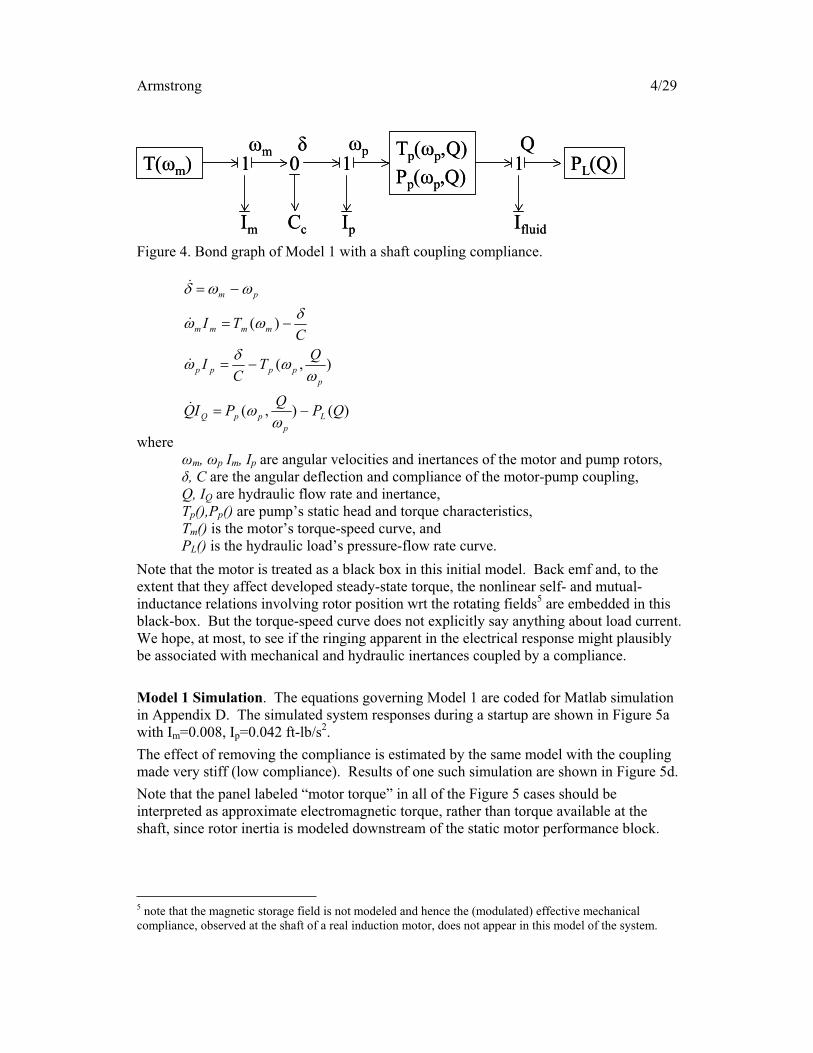
The system can be readily modeled with a shaft coupling compliance and separate motor

and pump rotor inertias. Including the hydraulic inertia is also straightforward. The bond

graph representation is shown in Figure 4 and the governing equations are:

0 2 4 6 8 10 12 140

0.5

1pumpEfficiency=eta

0 2 4 6 8 10 12 140.5

1

1.5

2ndTorque=f'(flowCoeff)

0 2 4 6 8 10 12 140

0.1

0.2ndPressure=g'(flowCoeff)

Armstrong 4/29

Figure 4. Bond graph of Model 1 with a shaft coupling compliance.

)(),(

),(

)(

QPQ

PIQ

QT

CI

CTI

L

p

ppQ

p

pppp

mmmm

pm

where

m, p Im, Ip are angular velocities and inertances of the motor and pump rotors,

, C are the angular deflection and compliance of the motor-pump coupling,

Q, IQ are hydraulic flow rate and inertance,

Tp(),Pp() are pump’s static head and torque characteristics,

Tm() is the motor’s torque-speed curve, and

PL() is the hydraulic load’s pressure-flow rate curve.

Note that the motor is treated as a black box in this initial model. Back emf and, to the

extent that they affect developed steady-state torque, the nonlinear self- and mutual-

inductance relations involving rotor position wrt the rotating fields5 are embedded in this

black-box. But the torque-speed curve does not explicitly say anything about load current.

We hope, at most, to see if the ringing apparent in the electrical response might plausibly

be associated with mechanical and hydraulic inertances coupled by a compliance.

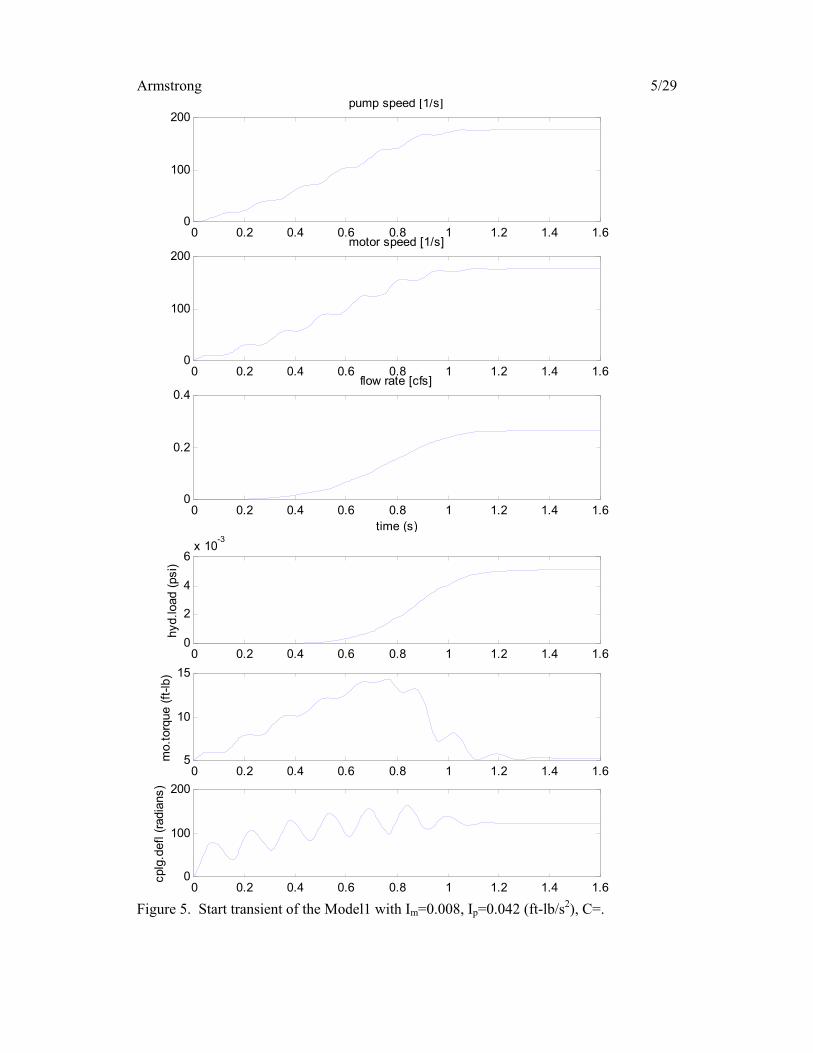
Model 1 Simulation. The equations governing Model 1 are coded for Matlab simulation

in Appendix D. The simulated system responses during a startup are shown in Figure 5a

with Im=0.008, Ip=0.042 ft-lb/s2.

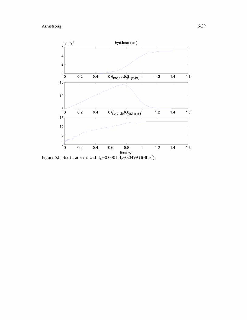
The effect of removing the compliance is estimated by the same model with the coupling

made very stiff (low compliance). Results of one such simulation are shown in Figure 5d.

Note that the panel labeled “motor torque” in all of the Figure 5 cases should be

interpreted as approximate electromagnetic torque, rather than torque available at the

shaft, since rotor inertia is modeled downstream of the static motor performance block.

5 note that the magnetic storage field is not modeled and hence the (modulated) effective mechanical

compliance, observed at the shaft of a real induction motor, does not appear in this model of the system.

T( m) 1 0

CcIm

1

Ip

Tp( p,Q)

Pp( p,Q)1

Ifluid

PL(Q)m p Q

T( m) 1 0

CcIm

1

Ip

Tp( p,Q)

Pp( p,Q)1

Ifluid

PL(Q)m p Q

Armstrong 5/29

Figure 5. Start transient of the Model1 with Im=0.008, Ip=0.042 (ft-lb/s2), C=.

0 0.2 0.4 0.6 0.8 1 1.2 1.4 1.60

100

200pump speed [1/s]

0 0.2 0.4 0.6 0.8 1 1.2 1.4 1.60

100

200motor speed [1/s]

0 0.2 0.4 0.6 0.8 1 1.2 1.4 1.60

0.2

0.4flow rate [cfs]

time (s)

0 0.2 0.4 0.6 0.8 1 1.2 1.4 1.60

2

4

6x 10

-3

hyd.load (

psi)

0 0.2 0.4 0.6 0.8 1 1.2 1.4 1.65

10

15

mo.t

orq

ue (

ft-lb)

0 0.2 0.4 0.6 0.8 1 1.2 1.4 1.60

100

200

cplg

.defl (

radia

ns)

Armstrong 6/29

Figure 5d. Start transient with Im=0.0001, Ip=0.0499 (ft-lb/s2).

0 0.2 0.4 0.6 0.8 1 1.2 1.4 1.60

2

4

6x 10

-3 hyd.load (psi)

0 0.2 0.4 0.6 0.8 1 1.2 1.4 1.65

10

15mo.torque (ft-lb)

0 0.2 0.4 0.6 0.8 1 1.2 1.4 1.60

5

10

15cplg.defl (radians)

time (s)

Armstrong 7/29

Model 2. The ringing obtained in the simulation of Figure 5, which involved shaft

compliance, is similar to the observed ringing depicted in Figure 1. However, it is not

quite plausible that—even during the brief period of startup when the motor develops peak

torque—a shaft coupler would deflect 10’s or 100’s of radians! We expect that similar

responses might be obtained by inserting a suitable compliance at any one of several other

points in the system. In fact, we know that change in flux linkage with shaft position

appears as a mechanical compliance and a given compliance inserted at this bond-graph

location will produce the slowest and largest oscillations because it puts all of the

significant (mechanical and hydraulic) inertances downstream.

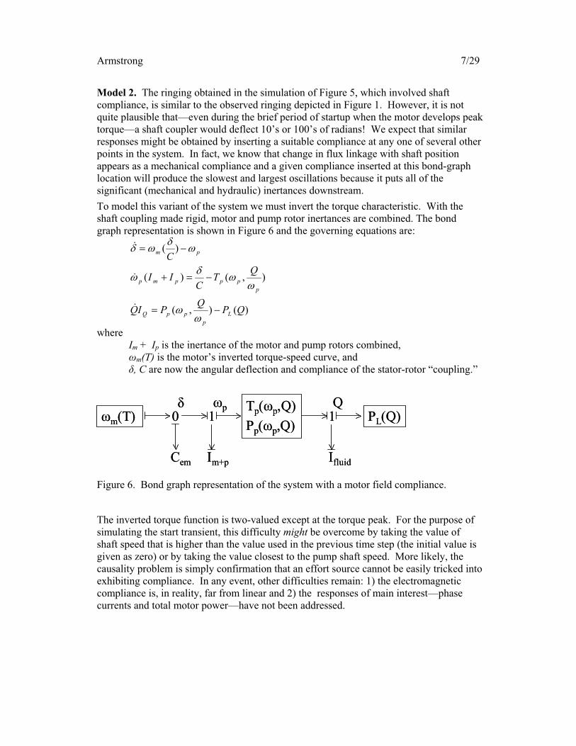
To model this variant of the system we must invert the torque characteristic. With the

shaft coupling made rigid, motor and pump rotor inertances are combined. The bond

graph representation is shown in Figure 6 and the governing equations are:

)(),(

),()(

)(

QPQ

PIQ

QT

CII

C

L

p

ppQ

p

pppmp

pm

where

Im + Ip is the inertance of the motor and pump rotors combined,

m(T) is the motor’s inverted torque-speed curve, and

, C are now the angular deflection and compliance of the stator-rotor “coupling.”

Figure 6. Bond graph representation of the system with a motor field compliance.

The inverted torque function is two-valued except at the torque peak. For the purpose of

simulating the start transient, this difficulty might be overcome by taking the value of

shaft speed that is higher than the value used in the previous time step (the initial value is

given as zero) or by taking the value closest to the pump shaft speed. More likely, the

causality problem is simply confirmation that an effort source cannot be easily tricked into

exhibiting compliance. In any event, other difficulties remain: 1) the electromagnetic

compliance is, in reality, far from linear and 2) the responses of main interest—phase

currents and total motor power—have not been addressed.

m(T) 0

Cem

1

Im+p

Tp( p,Q)

Pp( p,Q)1

Ifluid

PL(Q)p Q

m(T) 0

Cem

1

Im+p

Tp( p,Q)

Pp( p,Q)1

Ifluid

PL(Q)p Q

Armstrong 8/29

Induction Motor Model. Since model 2 faces a number of difficulties, the approach of

using a linear mechanical compliance to approximate the air-gap flux to rotor perturbation

relation was abandoned in favor of using a more realistic and informative motor model.

Standard 3-phase induction motor designs have multiple stator polls (most commonly 2 or

4 poles per phase) and a smooth rotor with a distributed “winding” such that the current in

each rotor bar is distinct. The apparent system order is depressingly large. If one

considers air gap flux the situation is somewhat better. However, a transformation

developed in the 1920’s [Park] that allows the electrical elements to be modeled in terms

of one complex stator flow-effort pair (iqds,vqds) and one complex rotor flow-effort pair

(iqdr,vqdr) has been used ever since, with variations [Stanley, Kron, Krause, Karnopp,

Breedveld], to simulate dynamic performance of induction and synchronous machines.

The assumptions commonly made in the analysis of 3-phase, line-powered machines are

1) balanced construction and excitation,

2) linear magnetics (to be relaxed later), and

3) sinusoidal distribution of air-gap flux.

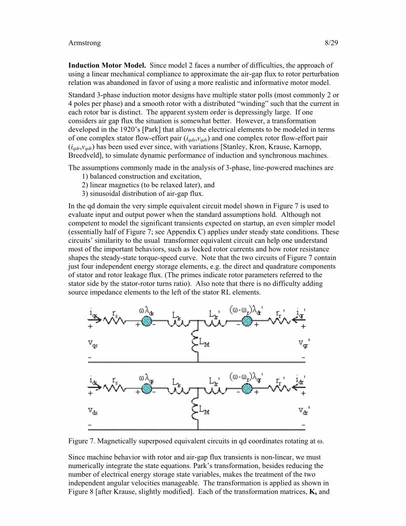
In the qd domain the very simple equivalent circuit model shown in Figure 7 is used to

evaluate input and output power when the standard assumptions hold. Although not

competent to model the significant transients expected on startup, an even simpler model

(essentially half of Figure 7; see Appendix C) applies under steady state conditions. These

circuits’ similarity to the usual transformer equivalent circuit can help one understand

most of the important behaviors, such as locked rotor currents and how rotor resistance

shapes the steady-state torque-speed curve. Note that the two circuits of Figure 7 contain

just four independent energy storage elements, e.g. the direct and quadrature components

of stator and rotor leakage flux. (The primes indicate rotor parameters referred to the

stator side by the stator-rotor turns ratio). Also note that there is no difficulty adding

source impedance elements to the left of the stator RL elements.

Figure 7. Magnetically superposed equivalent circuits in qd coordinates rotating at .

Since machine behavior with rotor and air-gap flux transients is non-linear, we must

numerically integrate the state equations. Park’s transformation, besides reducing the

number of electrical energy storage state variables, makes the treatment of the two

independent angular velocities manageable. The transformation is applied as shown in

Figure 8 [after Krause, slightly modified]. Each of the transformation matrices, Ks and

Armstrong 9/29

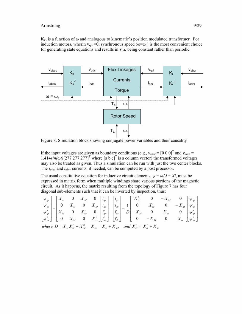
Kr, is a function of and analogous to kinematic’s position modulated transformer. For

induction motors, wherin vqdr=0, synchronous speed ( = e) is the most convenient choice

for generating state equations and results in vqds being constant rather than periodic.

Figure 8. Simulation block showing conjugate power variables and their causality

If the input voltages are given as boundary conditions (e.g., vabcr = [0 0 0]T and vabcr =

1.414sin( t)[277 277 277]T where [a b c]

T is a column vector) the transformed voltages

may also be treated as given. Thus a simulation can be run with just the two center blocks.

The iabcs and iabcr currents, if needed, can be computed by a post processor.

The usual constitutive equation for inductive circuit elements, = Li = Xi, must be

expressed in matrix form when multiple windings share various portions of the magnetic

circuit. As it happens, the matrix resulting from the topology of Figure 7 has four

diagonal sub-elements such that it can be inverted by inspection, thus:

Ks

Ks-1

Kr

Kr-1

Flux Linkages

Currents

Torque

vqds

iqds iqdr

vqdrvabcs

iabcs iadcr

vabcr

Rotor Speed

TL

Te

= e

r

r

mlrrrmlsssmrrss

dr

qr

ds

qs

ssM

ssM

Mrr

Mrr

dr

qr

ds

qs

dr

qr

ds

qs

rrM

rrM

Mss

Mss

dr

qr

ds

qs

XXXandXXXXXXDwhere

XX

XX

XX

XX

D

i

i

i

i

i

i

i

i

XX

XX

XX

XX

,,

00

00

00

00

1

00

00

00

00

2

Armstrong 10/29

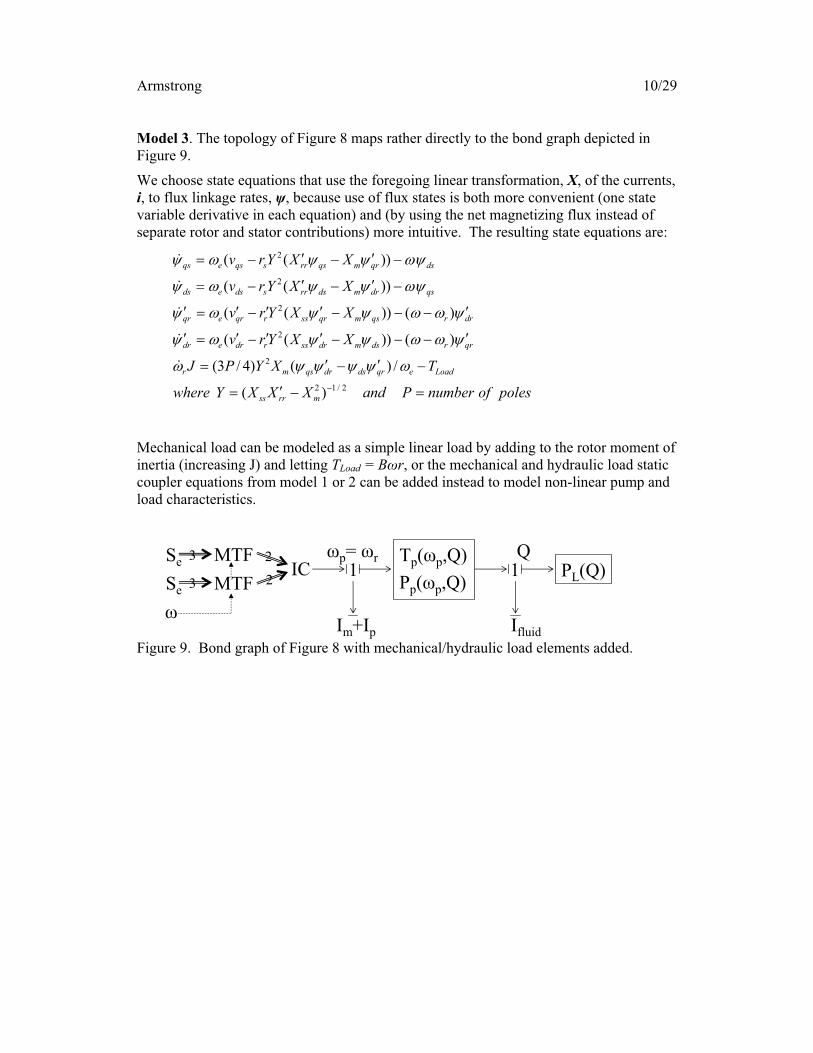
Model 3. The topology of Figure 8 maps rather directly to the bond graph depicted in

Figure 9.

We choose state equations that use the foregoing linear transformation, X, of the currents,

i, to flux linkage rates, , because use of flux states is both more convenient (one state

variable derivative in each equation) and (by using the net magnetizing flux instead of

separate rotor and stator contributions) more intuitive. The resulting state equations are:

Mechanical load can be modeled as a simple linear load by adding to the rotor moment of

inertia (increasing J) and letting TLoad = B r, or the mechanical and hydraulic load static

coupler equations from model 1 or 2 can be added instead to model non-linear pump and

load characteristics.

Figure 9. Bond graph of Figure 8 with mechanical/hydraulic load elements added.

polesofnumberPandXXXYwhere

TXYPJ

XXYrv

XXYrv

XXYrv

XXYrv

mrrss

Loadeqrdsdrqsmr

qrrdsmdrssrdredr

drrqsmqrssrqreqr

qsdrmdsrrsdseds

dsqrmqsrrsqseqs

2/12

2

2

2

2

2

)(

/)()4/3(

)())((

)())((

))((

))((

Se1

Im+Ip

Tp( p,Q)

Pp( p,Q)1

Ifluid

PL(Q)p= r Q

ICMTF

MTFSe

3 2

23

Armstrong 11/29

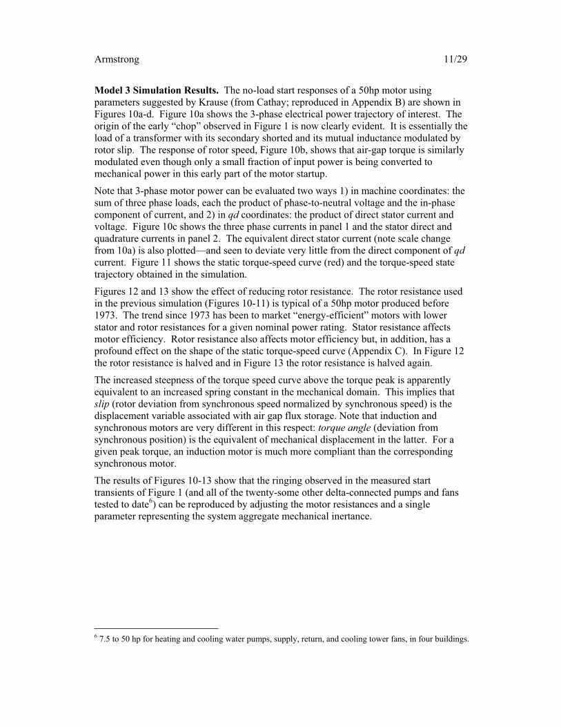
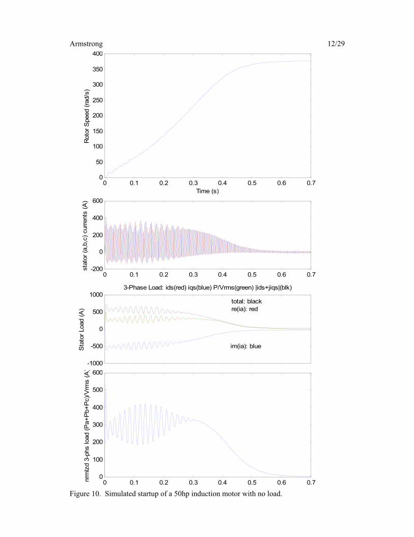
Model 3 Simulation Results. The no-load start responses of a 50hp motor using

parameters suggested by Krause (from Cathay; reproduced in Appendix B) are shown in

Figures 10a-d. Figure 10a shows the 3-phase electrical power trajectory of interest. The

origin of the early “chop” observed in Figure 1 is now clearly evident. It is essentially the

load of a transformer with its secondary shorted and its mutual inductance modulated by

rotor slip. The response of rotor speed, Figure 10b, shows that air-gap torque is similarly

modulated even though only a small fraction of input power is being converted to

mechanical power in this early part of the motor startup.

Note that 3-phase motor power can be evaluated two ways 1) in machine coordinates: the

sum of three phase loads, each the product of phase-to-neutral voltage and the in-phase

component of current, and 2) in qd coordinates: the product of direct stator current and

voltage. Figure 10c shows the three phase currents in panel 1 and the stator direct and

quadrature currents in panel 2. The equivalent direct stator current (note scale change

from 10a) is also plotted—and seen to deviate very little from the direct component of qd

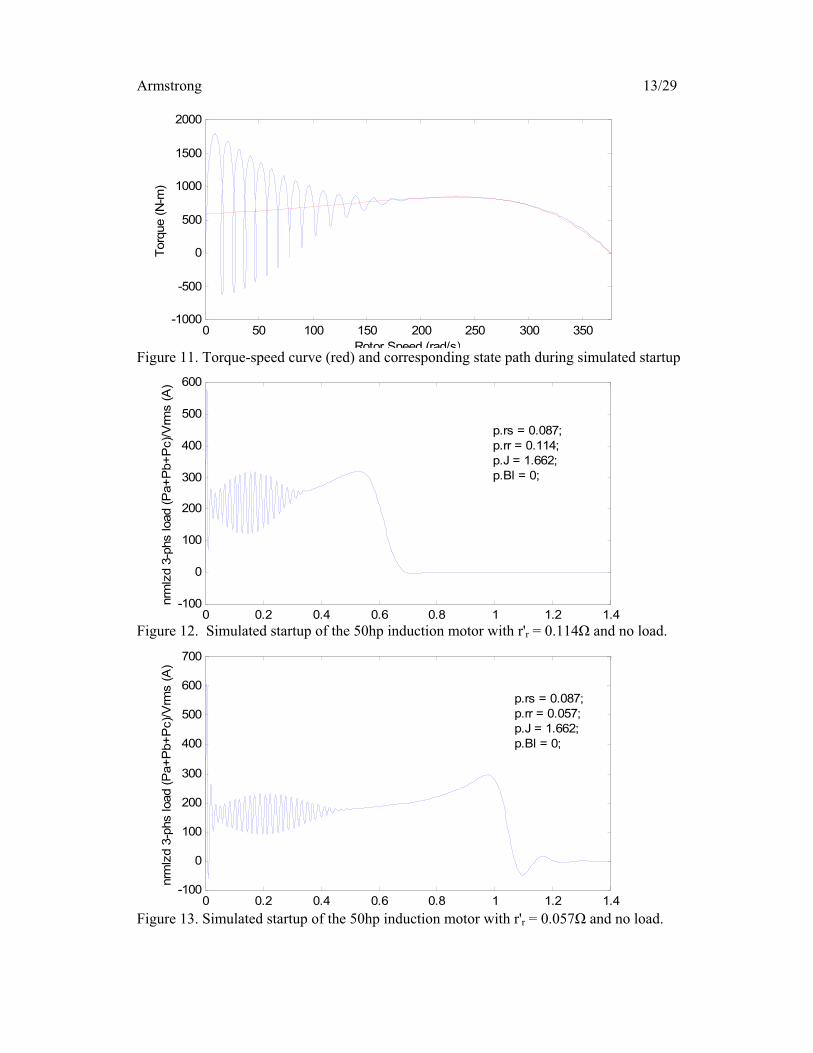
current. Figure 11 shows the static torque-speed curve (red) and the torque-speed state

trajectory obtained in the simulation.

Figures 12 and 13 show the effect of reducing rotor resistance. The rotor resistance used

in the previous simulation (Figures 10-11) is typical of a 50hp motor produced before

1973. The trend since 1973 has been to market “energy-efficient” motors with lower

stator and rotor resistances for a given nominal power rating. Stator resistance affects

motor efficiency. Rotor resistance also affects motor efficiency but, in addition, has a

profound effect on the shape of the static torque-speed curve (Appendix C). In Figure 12

the rotor resistance is halved and in Figure 13 the rotor resistance is halved again.

The increased steepness of the torque speed curve above the torque peak is apparently

equivalent to an increased spring constant in the mechanical domain. This implies that

slip (rotor deviation from synchronous speed normalized by synchronous speed) is the

displacement variable associated with air gap flux storage. Note that induction and

synchronous motors are very different in this respect: torque angle (deviation from

synchronous position) is the equivalent of mechanical displacement in the latter. For a

given peak torque, an induction motor is much more compliant than the corresponding

synchronous motor.

The results of Figures 10-13 show that the ringing observed in the measured start

transients of Figure 1 (and all of the twenty-some other delta-connected pumps and fans

tested to date6) can be reproduced by adjusting the motor resistances and a single

parameter representing the system aggregate mechanical inertance.

6 7.5 to 50 hp for heating and cooling water pumps, supply, return, and cooling tower fans, in four buildings.

Armstrong 12/29

0 0.1 0.2 0.3 0.4 0.5 0.6 0.70

50

100

150

200

250

300

350

400

Time (s)

Roto

r S

peed (

rad/s

)

0 0.1 0.2 0.3 0.4 0.5 0.6 0.7-200

0

200

400

600

sta

tor

(a,b

,c)

curr

ents

(A

)

-1000

-500

0

500

1000

Sta

tor

Load (

A)

3-Phase Load: ids(red) iqs(blue) P/Vrms(green) |ids+jiqs|(blk)

total: black

re(ia): red

im(ia): blue

0 0.1 0.2 0.3 0.4 0.5 0.6 0.70

100

200

300

400

500

600

nrm

lzd 3

-phs load (

Pa+

Pb+

Pc)/

Vrm

s (

A)

Figure 10. Simulated startup of a 50hp induction motor with no load.

Armstrong 13/29

0 50 100 150 200 250 300 350-1000

-500

0

500

1000

1500

2000

Rotor Speed (rad/s)

Torq

ue (

N-m

)

Figure 11. Torque-speed curve (red) and corresponding state path during simulated startup

0 0.2 0.4 0.6 0.8 1 1.2 1.4-100

0

100

200

300

400

500

600

nrm

lzd 3

-phs load (

Pa+

Pb+

Pc)/

Vrm

s (

A)

p.rs = 0.087;

p.rr = 0.114;

p.J = 1.662;

p.Bl = 0;

Figure 12. Simulated startup of the 50hp induction motor with r'r = 0.114 and no load.

0 0.2 0.4 0.6 0.8 1 1.2 1.4-100

0

100

200

300

400

500

600

700

nrm

lzd 3

-phs load (

Pa+

Pb+

Pc)/

Vrm

s (

A)

p.rs = 0.087;

p.rr = 0.057;

p.J = 1.662;

p.Bl = 0;

Figure 13. Simulated startup of the 50hp induction motor with r'r = 0.057 and no load.

Armstrong 14/29

0 50 100 150 200 250 300 350-600

-400

-200

0

200

400

600

800

1000

Rotor Speed (rad/s)

Torq

ue (

N-m

)

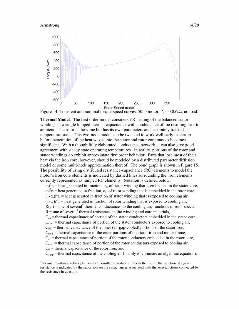
Figure 14. Transient and nominal torque-speed curves, 50hp motor, r'r = 0.057 , no load.

Thermal Model. The first order model considers i2R heating of the balanced stator

windings as a single lumped thermal capacitance with conductance of the resulting heat to

ambient. The rotor is the same but has its own parameters and separately tracked

temperature state. This two-node model can be tweaked to work well early in startup

before penetration of the heat waves into the stator and rotor core masses becomes

significant. With a thoughtfully elaborated conductance network, it can also give good

agreement with steady state operating temperatures. In reality, portions of the rotor and

stator windings do exhibit approximate first order behavior. Parts that lose most of their

heat via the iron core, however, should be modeled by a distributed parameter diffusion

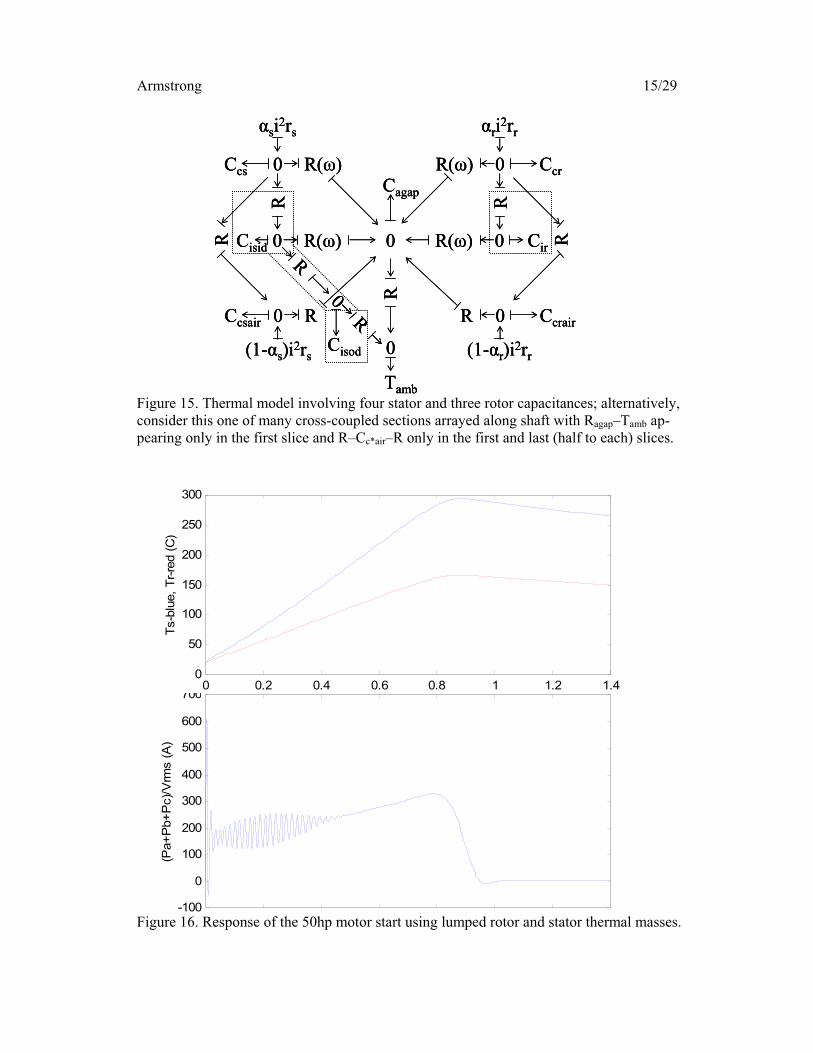
model or some multi-node approximation thereof. The bond graph is shown in Figure 15.

The possibility of using distributed resistance-capacitance (RC) elements to model the

motor’s iron core elements is indicated by dashed lines surrounding the iron elements

currently represented as lumped RC elements. Notation is defined below:

si2rs = heat generated in fraction, s, of stator winding that is embedded in the stator core,

ri2rr = heat generated in fraction, r, of rotor winding that is embedded in the rotor core,

(1- s)i2rs = heat generated in fraction of stator winding that is exposed to cooling air,

(1- r)i2rr = heat generated in fraction of rotor winding that is exposed to cooling air,

R( ) = one of several7 thermal conductances to the cooling air, functions of rotor speed,

R = one of several7 thermal resistances in the winding and core materials,

Ccs = thermal capacitance of portion of the stator conductors embedded in the stator core,

Ccsair = thermal capacitance of portion of the stator conductors exposed to cooling air,

Cisid = thermal capacitance of the inner (air gap-cooled) portions of the stator iron,

Cisod = thermal capacitance of the outer portions of the stator iron and motor frame,

Ccr = thermal capacitance of portion of the rotor conductors embedded in the rotor core,

Ccrair = thermal capacitance of portion of the rotor conductors exposed to cooling air,

Cir = thermal capacitance of the rotor iron, and

Cagap = thermal capacitance of the cooling air (mainly to eliminate an algebraic equation).

7 thermal resistance subscripts have been omitted to reduce clutter in the figure; the function of a given

resistance is indicated by the subscripts on the capacitances associated with the zero junctions connected by

the resistance in question.

Armstrong 15/29

Figure 15. Thermal model involving four stator and three rotor capacitances; alternatively,

consider this one of many cross-coupled sections arrayed along shaft with Ragap–Tamb ap-

pearing only in the first slice and R–Cc*air–R only in the first and last (half to each) slices.

0 0.2 0.4 0.6 0.8 1 1.2 1.40

50

100

150

200

250

300

Ts-b

lue,

Tr-

red (

C)

-100

0

100

200

300

400

500

600

700

(Pa+

Pb+

Pc)/

Vrm

s (

A)

Figure 16. Response of the 50hp motor start using lumped rotor and stator thermal masses.

0Cisid R( ) 0 0 CirR( )

0Ccs R( ) 0 CcrR( )

R

RR

0Ccsair R

0

0 CcrairR

R R

(1- s)i2rs (1- r)i

2rr

ri2rrsi

2rs

R

R

Tamb

0

Cisod

Cagap


0Ccs R( ) 0 CcrR( )

R

RR

0Ccsair R

0

0 CcrairR

R R

(1- s)i2rs (1- r)i

2rr

ri2rrsi

2rs

R

R

Tamb

0

Cisod

Cagap


0Ccs R( ) 0 CcrR( )

R

RR

0Ccsair R

0

0 CcrairR

R R

(1- s)i2rs (1- r)i

2rr

ri2rrsi

2rs

R

RR

Tamb

0

Cisod

Cagap

Armstrong 16/29

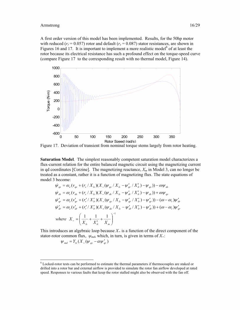
A first order version of this model has been implemented. Results, for the 50hp motor

with reduced (rr = 0.057) rotor and default (rs = 0.087) stator resistances, are shown in

Figures 16 and 17. It is important to implement a more realistic model8 of at least the

rotor because its electrical resistance has such a profound effect on the torque-speed curve

(compare Figure 17 to the corresponding result with no thermal model, Figure 14).

0 50 100 150 200 250 300 350-600

-400

-200

0

200

400

600

800

1000

Rotor Speed (rad/s)

Torq

ue (

N-m

)

Figure 17. Deviation of transient from nominal torque stems largely from rotor heating.

Saturation Model. The simplest reasonably competent saturation model characterizes a

flux-current relation for the entire balanced magnetic circuit using the magnetizing current

in qd coordinates [Corzine]. The magnetizing reactance, Xm in Model 3, can no longer be

treated as a constant, rather it is a function of magnetizing flux. The state equations of

model 3 become:

This introduces an algebraic loop because X= is a function of the direct component of the

stator-rotor common flux, md, which, in turn, is given in terms of X=:

8 Locked-rotor tests can be performed to estimate the thermal parameters if thermocouples are staked or

drilled into a rotor bar and external airflow is provided to simulate the rotor fan airflow developed at rated

speed. Responses to various faults that keep the rotor stalled might also be observed with the fan off.

1

111

)()))//()(/((

)()))//()(/((

)))//()(/((

)))//()(/((

mlrls

qrrdrlrdrlsdslrrdredr

drrqrlrqrlsqslrrqreqr

qsdslrdrlsdslssdseds

dsqslrqrlsqslssqseqs

XXXXwhere

XXXXrv

XXXXrv

XXXXrv

XXXXrv

)(( qrqslsmd XY

Armstrong 17/29

The non-linear reactance, Xm( md), could be implemented by table lookup but a safer

approach is to use the arctan function recommended by Corzine to avoid bad derivative

behavior. This simplest of saturation models ignores the fact that leakage inductances

become variable, increasing significantly at the onset of saturation.

Next Steps. Effects of saturation and thermal transient parameters need to be explored. A

test motor with known magnetic and thermal parameters is needed. A number of other

tasks should also be pursued.

For verification, the simulation results for A-phase direct and quadrature current and

power must be passed through the appropriate spectral envelope filter before comparing to

responses of the type depicted in Figure 1. We need to simulate a known9 system and, if

possible, one in which at least the piping circuit inertance and static characteristics can be

varied, e.g. by two shunt valves, one close to and one remote from the pump.

Measurements of rotor speed and pump pressure during startup would be very useful.

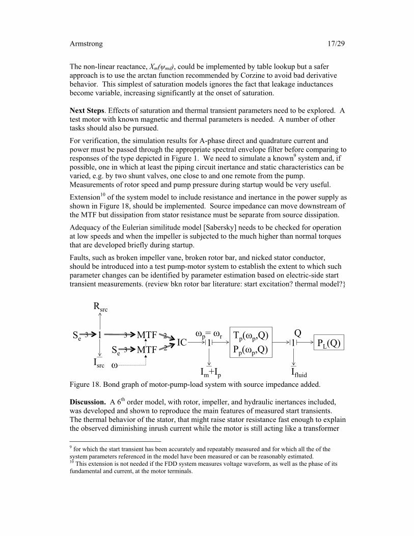
Extension10

of the system model to include resistance and inertance in the power supply as

shown in Figure 18, should be implemented. Source impedance can move downstream of

the MTF but dissipation from stator resistance must be separate from source dissipation.

Adequacy of the Eulerian similitude model [Sabersky] needs to be checked for operation

at low speeds and when the impeller is subjected to the much higher than normal torques

that are developed briefly during startup.

Faults, such as broken impeller vane, broken rotor bar, and nicked stator conductor,

should be introduced into a test pump-motor system to establish the extent to which such

parameter changes can be identified by parameter estimation based on electric-side start

transient measurements. (review bkn rotor bar literature: start excitation? thermal model?}

Figure 18. Bond graph of motor-pump-load system with source impedance added.

Discussion. A 6th

order model, with rotor, impeller, and hydraulic inertances included,

was developed and shown to reproduce the main features of measured start transients.

The thermal behavior of the stator, that might raise stator resistance fast enough to explain

the observed diminishing inrush current while the motor is still acting like a transformer

9 for which the start transient has been accurately and repeatably measured and for which all the of the

system parameters referenced in the model have been measured or can be reasonably estimated. 10 This extension is not needed if the FDD system measures voltage waveform, as well as the phase of its

fundamental and current, at the motor terminals.

Se

Im+Ip

Tp( p,Q)

Pp( p,Q)1

Ifluid

PL(Q)p= r Q

ICMTF

MTFSe

3 2

231

13

Isrc

Rsrc

Armstrong 18/29

with its secondary shorted, has not been modeled yet. The state equations that account for

saturation have been developed but not yet coded in Matlab.

The proposed FDD system measures all three phase currents and voltages, making

detection of electrical imbalances in both the power supply and load very straightforward.

This study therefore focused on mechanical and hydraulic aspects of the system to explore

the extent to which they might be characterized and monitored by the electric-side

measurements. Two derived responses, total real and total reactive motor power, were

found, as expected based on the qd (Park’s) transformation, to be useful, given balanced

electric-side conditions, for these purposes.

The effects of parameter changes were explored. The following parameters had effects

that were found to be important:

stator and rotor winding resistances

lumped mechanical/hydraulic inertance

dominant compliance (function of motor parameters)

stator and rotor thermal capacitances

When a compliant coupling (belt or flexible shaft coupling) is added between the motor

and fan or pump, the rotor inertance is decoupled from the downstream inertances by the

compliance. Preliminary simulations indicate that the additional poles are too highly

damped or too far from the real axis to be detected reliably from a typical start transient.

Future work should explore whether such poles might be detected from response to step

changes or impulses in excitation during normal run conditions, e.g. brief power

interruption with stator leads open or shorted.

There may be cases where compliances in the hydraulic system are significant to the

observed responses. Further field testing is needed to explore this hypothesis.

The most practical approach to FDD appears to involve a priori data. Blocked-rotor and

no-load run-up responses are easily obtained by 1) making modest extensions of the FDD

monitoring system’s software and 2) calling for such tests as part of building

commissioning. The static torque curve is important, particularly the slope around

nominal steady-state load. It is not clear if the curves given by manufacturers are

sufficiently reliable and, if not, whether reliable electrical parameters (mutual inductance,

rotor and stator resistance and leakage inductance) can be obtained in the field. The

possibility of obtaining a reasonable static torque-speed curve during commissioning

seems tenuous but may be worth exploring.

Note that there are two important reasons to integrate the FDD system with the control

system. First, it can simplify building commissioning and, second, it enables an active

testing component of FDD—i.e., extends passive-monitoring-based FDD by enabling

automated active testing processes. There is a third reason that does not necessarily apply

to pumps but would certainly apply to other pieces of the plant, e.g., chillers: model-based

FDD and model-based control can share the same model.

To aid further development and refinement of on-line-model based FDD, it may be

important to have the 3-phase, high bandwidth monitoring subsystem (under

development) output the unfiltered (or lightly filtered) 3-phase power signal, sampled at a

fairly high frequency (e.g. 900-1200 Hz), in addition to the spectral envelopes output by

the preprocessor stage in the current single-phase implementation.

Armstrong 19/29

The problem of tracking shaft speed during transients is a difficult one [Velez-Reyes,

Shaw 1999] that has not been addressed here. We have so far focused on FDD

measurements, models and approaches that do not require a measurement or estimate of

shaft speed. Belt driven shaft speeds, if needed, can be estimated in steady operation

from the spectral envelope data [5/01 CEC progress report] and might also be reliably

estimated for direct coupled pumps were the 3-phase power measurement, discussed

above, made available. It would be reasonable to measure transient shaft speeds during

commissioning if there is sufficient value in doing so. These are additional possibilities to

be explored in the future.

References.

Breedveld, P.C., 2001. A generic dynamic model of multiphase electromechanical

transduction in rotating machinery, Proc. WESIC.

Brown, F.T. 2001. Engineering System Dynamics, Marcel Dekker, New York..

Cathay, J.J., et al, 1973. Transient load model of an induction machine, IEEE Trans. PAS92(1399-1406).

Corzine, K.A., et al, 1998. An improved method for incorporating magnetic saturation in

the q-d synchronous machine model, IEEE Trans. Energy Conversion, 13(3) pp.270-275.

Karnopp, D. 1991. State functions and bond graph dynamic models for rotary, multi-

winding electrical machines, J. Franklin Institute, 328(1) pp.45-54.

Krause, P.C., et al, 2002. Analysis of Electric Machinery and Drive Systems, 2nd

Edition,

IEEE Press, Piscataway, NJ.

Kron, G., 1951. Equivalent Circuits of Electric Machinery, J. Wiley and Sons, NY.

Laughman, C.R., et al, 2002. Advanced non-intrusive monitoring of electric loads,

submitted October 2002 to IEEE CAP.

Leeb, S.B. and S.R. Shaw, 1994. Harmonic estimates for transient event detection, IEEEUPEC.

Ong, C-M. 2998. Dynamic Simulation of Electric Machinery, Prentice-Hall, NJ.

Park, R.H., 1929. A two-reaction theory of synchronous machines—generalized method

of analysis, part I; AIEE Trans. 48(716-727).

Sabersky, R.H. and A.J. Acosta, 1971. Fluid Flow, MacMillan, NY.

Sen Gupta, D.P. and J.W. Lynn, 1980. Electrical Machine Dynamics, MacMillan.

Shaw, S.R., and S.B.Leeb, 1999. Identification of Induction Motor Parameters from

Transient Stator Current Measurements, IEEE Trans. Industrial Electronics, 46(1) pp.139-

149.

Shaw, S.R., et al, 2000. A power quality prediction system, IEEE Trans. Industrial Electronics, 47(3) pp.511-517.

Tavner, P.J. and J. Penman, 1987. Condition Monitoring of Electric Machines, Wiley.

Velez-Reyes, M., et al, 1989. Recursive speed and parameter estimation for induction

machines, Proc. IEEE-IAS Annual Meeting, pp.607-611.

Armstrong 20/29

Appendix A: Spectral Envelope Filter (after Laughman)

The spectral envelope filter is an ideal demodulator for amplitude modulated signals. The

ideal demodulator assumes a known carrier frequency. The carrier of interest for analysis

of electric loads on the North American grid is, of course, 60Hz. For nonlinear loads,

useful information may be lost with the 60Hz filter. In this case, signals obtained by

spectral envelope filters applied at harmonics of 60Hz will contain additional information.

If i(t) is the current of a load driven by a voltage, e(t) = Vsin( t), the direct and quadrature

kth

harmonic spectral envelopes are given by

2

)cos()(2

)(

)sin()(2

)(

Twhere

dkxT

tb

dkxT

ta

t

Ttk

t

Ttk

Additional smoothing can be obtained (albeit with additional loss of information) by using

integer multiples of T. {Matlab function to implement spectral envelope filter goes here.}

Appendix B. Motor and Pump Data

Table B-1. Bell and Gosset 1510 Series, Model 6E, 10.5” impeller. Data scaled from

B&G published performance chart at 1770 rpm.

Gpm ft.WC hp Eff

420 102 25 44

520 101.9 26.8 50

690 101.6 29.9 60

930 101 34.2 70

1070 99.6 36.5 75

1250 97.7 38.9 80

1465 94.2 41.6 85

1650 90.3 43.5 86

1895 82.5 45.9 87

2040 77 46.4 86

2125 73.5 46.7 85

2295 64 46.6 80

2415 57.5 46.3 75

Table B-2. Induction motor parameters; Cathay (1982, Table 4.10 in Krause), Ong (1998)

Machine Rating TB IB Rs Xls XM X´lr R´r J

Hp V Rpm N-m A kg-m2

V* XM

hp

3 220 1710 11.9 5.8 .435 .754 26.13 .754 .816 .089

20 220 1748 79.2 49.7 .1062 .2145 5.834 .2145 .0764 2.8

50 460 1705 198 46.8 .087 .302 13.08 .302 .228 1.662

500 2300 1773 1980 93.6 .262 1.206 54.02 1.206 .187 11.06

2250 2300 1786 8900 421.2 .029 .226 13.04 .226 .022 63.87

Armstrong 21/29

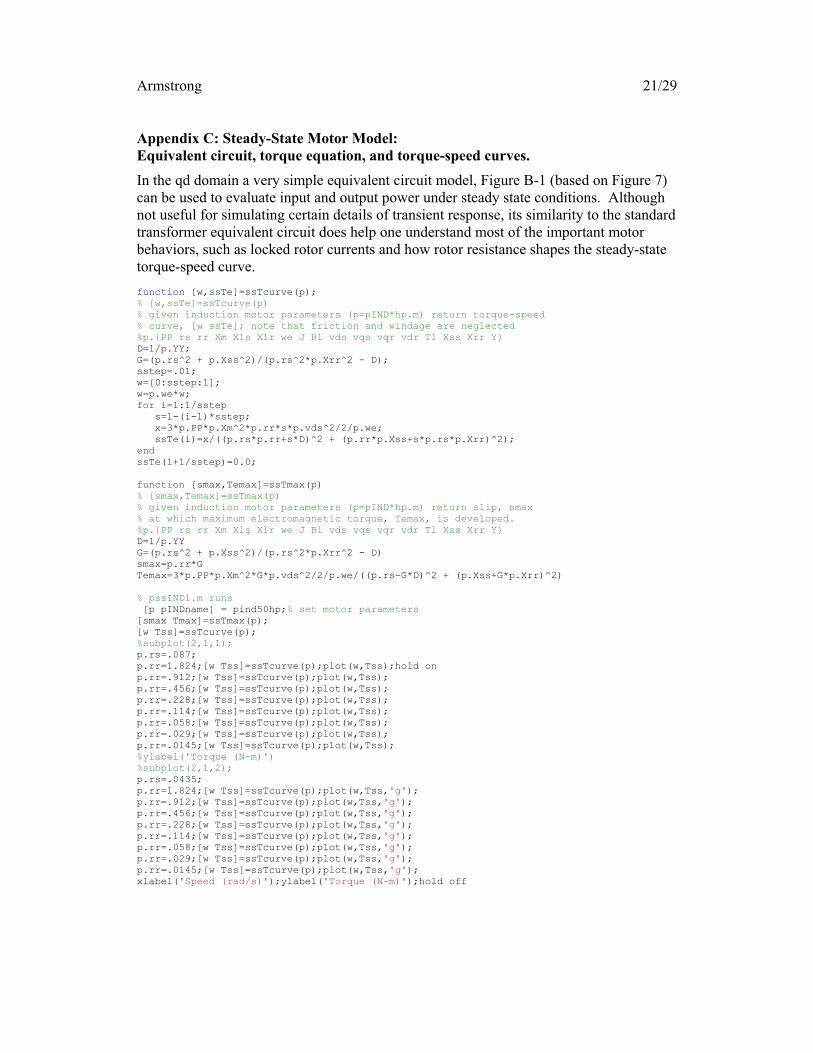
Appendix C: Steady-State Motor Model:

Equivalent circuit, torque equation, and torque-speed curves.

In the qd domain a very simple equivalent circuit model, Figure B-1 (based on Figure 7)

can be used to evaluate input and output power under steady state conditions. Although

not useful for simulating certain details of transient response, its similarity to the standard

transformer equivalent circuit does help one understand most of the important motor

behaviors, such as locked rotor currents and how rotor resistance shapes the steady-state

torque-speed curve.

function [w,ssTe]=ssTcurve(p);

% [w,ssTe]=ssTcurve(p)

% given induction motor parameters (p=pIND*hp.m) return torque-speed

% curve, [w ssTe]; note that friction and windage are neglected

%p.{PP rs rr Xm Xls Xlr we J Bl vds vqs vqr vdr Tl Xss Xrr Y}

D=1/p.YY;

G=(p.rs^2 + p.Xss^2)/(p.rs^2*p.Xrr^2 - D);

sstep=.01;

w=[0:sstep:1];

w=p.we*w;

for i=1:1/sstep

s=1-(i-1)*sstep;

x=3*p.PP*p.Xm^2*p.rr*s*p.vds^2/2/p.we;

ssTe(i)=x/((p.rs*p.rr+s*D)^2 + (p.rr*p.Xss+s*p.rs*p.Xrr)^2);

end

ssTe(1+1/sstep)=0.0;

function [smax,Temax]=ssTmax(p)

% [smax,Temax]=ssTmax(p)

% given induction motor parameters (p=pIND*hp.m) return slip, smax

% at which maximum electromagnetic torque, Temax, is developed.

%p.{PP rs rr Xm Xls Xlr we J Bl vds vqs vqr vdr Tl Xss Xrr Y}

D=1/p.YY

G=(p.rs^2 + p.Xss^2)/(p.rs^2*p.Xrr^2 - D)

smax=p.rr*G

Temax=3*p.PP*p.Xm^2*G*p.vds^2/2/p.we/((p.rs-G*D)^2 + (p.Xss+G*p.Xrr)^2)

% pssIND1.m runs

[p pINDname] = pind50hp;% set motor parameters

[smax Tmax]=ssTmax(p);

[w Tss]=ssTcurve(p);

%subplot(2,1,1);

p.rs=.087;

p.rr=1.824;[w Tss]=ssTcurve(p);plot(w,Tss);hold on

p.rr=.912;[w Tss]=ssTcurve(p);plot(w,Tss);







%ylabel('Torque (N-m)')

%subplot(2,1,2);

p.rs=.0435;

p.rr=1.824;[w Tss]=ssTcurve(p);plot(w,Tss,'g');

p.rr=.912;[w Tss]=ssTcurve(p);plot(w,Tss,'g');







xlabel('Speed (rad/s)');ylabel('Torque (N-m)');hold off

Armstrong 22/29

0 50 100 150 200 250 300 350 4000

100

200

300

400

500

600

700

800

900

1000

Speed (rad/s)

Torq

ue (

N-m

)

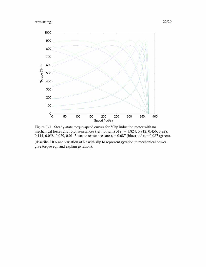
Figure C-1. Steady-state torque-speed curves for 50hp induction motor with no

mechanical losses and rotor resistances (left to right) of r´r = 1.824, 0.912, 0.456, 0.228,

0.114, 0.058, 0.029, 0.0145; stator resistances are rs = 0.087 (blue) and rs = 0.087 (green).

(describe LRA and variation of Rr with slip to represent gyration to mechanical power.

give torque eqn and explain gyration).

Armstrong 23/29

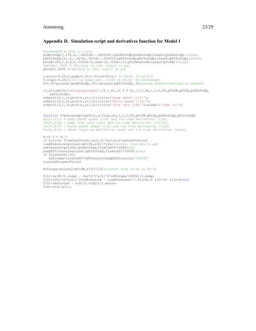
Appendix D. Simulation script and derivatives function for Model 1

%simpump02.m 2002.11.11pra

pndPofndQ=[.174,0,-.000328,-.0000281];pndPofndQ=pndPofndQ(length(pndPofndQ):-1:1);

pEffofndQ=[0,.2,-.0238,.00158,-.000053];pEffofndQ=pEffofndQ(length(pEffofndQ):-1:1);

pTofW=[60,1.2,0,0,-1453e-9,182e-10,-635e-13];pTofW=pTofW(length(pTofW):-1:1);

%pPofQ=[.0005 0 30];%arg in cfs, result in psi

pPofQ=[.0005 0 0];%arg in cfs, result in psi

I.motor=0.02;I.pump=0.03;I.fluid=8310;% ft-lb/2; lb-s2/ft5

C.coupl=0.05;%1/10 is compliant, 1/100 is stiff [ft-lb/radian]

T0=.01*polyval(pndPofndQ,.01)/polyval(pEffofndQ,.01);%else Q/eff=undefined at speed=0

[t,y]=ode15s('motorpumpload02',[0 1.6],[0 0 0 0],[],1.94,1,I,C,T0,pTofW,pPofQ,pndPofndQ,

pEffofndQ);

subplot(3,1,1);plot(t,y(:,1));title('pump speed [1/s]');

subplot(3,1,2);plot(t,y(:,3));title('motor speed [1/s]');

subplot(3,1,3);plot(t,y(:,2));title('flow rate [cfs]');xlabel('time (s)');

function f=motorpumpload02(t,x,flag,rho,L,I,C,T0,pTofW,pPofQ,pndPofndQ,pEffofndQ)

%x(1),f(1) = pump shaft speed [1/s] and its time derivative [1/s2]

%x(2),f(2) = pump flow rate [cfs] and its time derivative [ft3/s2]

%x(3),f(3) = motor shaft speed [1/s] and its time derivative [1/s2]

%x(4),f(4) = shaft coupling deflection [rad] and its time derivative [rad/s]

f=[0 0 0 0]';

if x(1)>0; flowCoeff=x(2)/x(1)/L^3;else;flowCoeff=0;end

loadPressure=polyval(pPofQ,x(2))*144;%convert from psi to psf

ndPressure=polyval(pndPofndQ,flowCoeff*10000);%g'

pumpEfficiency=polyval(pEffofndQ,flowCoeff*10000);%eta

if flowCoeff>.01;

ndTorque=flowCoeff*ndPressure/pumpEfficiency;%10000f'

else;ndTorque=T0;end

moTorque=polyval(pTofW,x(3))/12;%convert from in-lb to ft-lb

f(1)=(x(4)/C.coupl - rho*L^5*x(1)^2*ndTorque/10000)/I.pump;

f(2)=(rho*(L*x(1))^2*ndPressure - loadPressure)/I.fluid;if f(2)<0; f(2)=0;end

f(3)=(moTorque - x(4)/C.coupl)/I.motor;

f(4)=x(3)-x(1);

Armstrong 24/29

Appendix E. Simulation script and derivatives function for Model 2 %simpump03.m 2002.11.12pra



pTofW=[60,1.2,0,0,-1453e-9,182e-10,-635e-13];pTofW=pTofW(length(pTofW):-1:1);



n=length(pTofW)-1;

d1=pTofW(1:n);d1=d1.*[n:-1:1]

p=d1;p=roots(p);k=0;

for i=1:n-1;%eliminate infeasible roots

if imag(p(i))==0 & real(p(i))>0; k=k+1; p(k)=p(i);end

end

wmax=min(p(1:k));maxT=polyval(pTofW,wmax);

I.motor=0.02;I.pump=0.03;I.fluid=8310;% ft-lb/2; lb-s2/ft5

C.coupl=0.05;C.emag=0.05;%1/10 is compliant, 1/100 is stiff [ft-lb/radian]

T0=.01*polyval(pndPofndQ,.01)/polyval(pEffofndQ,.01);%else Q/eff=undefined at speed=0

[t,y]=ode15s('motorpumpload03',[0 1.6],[0 0

0],[],1.94,1,I,C,T0,pTofW,maxT,pPofQ,pndPofndQ,pEffofndQ)

% function f=motorpumpload01(t,x,flag,rho,L,I,T0,pTofW,pPofQ,pndPofndQ,pEffofndQ)

subplot(3,1,1);plot(t,y(:,1));title('pump speed [1/s]');

subplot(3,1,2);plot(t,y(:,3));title('motor speed [1/s]');

subplot(3,1,3);plot(t,y(:,2));title('flow rate [cfs]');xlabel('time (s)');

function f=motorpumpload03(t,x,flag,rho,L,I,C,T0,pTofW,maxT,pPofQ,pndPofndQ,pEffofndQ)

%x(1),f(1) = pump shaft speed [rad/s] and its time derivative [rad/s2]

%x(2),f(2) = pump flow rate [cfs] and its time derivative [ft3/s2]

%x(3),f(3) = field-rotor deflection [rad] and its time derivative [rad/s]

%global wm;%need initial guess on first call (previous value is fine for subsequent calls)

%another ploy that might work: use pump speed as the initial guess

f=[0 0 0]';

if x(1)>0; flowCoeff=x(2)/x(1)/L^3;else;flowCoeff=0;end

loadPressure=polyval(pPofQ,x(2))*144;%convert from psi to psf

ndPressure=polyval(pndPofndQ,flowCoeff*10000);%g'

pumpEfficiency=polyval(pEffofndQ,flowCoeff*10000);%eta

if flowCoeff>.01;

ndTorque=flowCoeff*ndPressure/pumpEfficiency;%10000f'

else;ndTorque=T0;end

moTorque=12*x(3)/C.emag; %convert from ft-lb to in-lb %=polyval(pTofW,x(3))/12;

%use Matlab fcn ROOTS and fact that wm>wmprev during start transient

p=pTofW; p(7)=p(7)-moTorque; p=roots(p); k=0;

for i=1:6; %eliminate infeasible (neg & complex) roots

if imag(p(i))==0 & real(p(i))>0; k=k+1; p(k)=p(i);end

end

[wm i]=min(p(1:k));

if moTorque>maxT; wm=min([p(1:i-1) p(i+1:k)]);end

if length(wm)~=1; disp([moTorque maxT i]);disp(p);disp(wm);error('moTorque,maxT,i,p,wm

(not scalar)');end

%if x(1)==0; wm=0; end

moTorque=moTorque/12

%SECANT METHOD will have trouble getting over torque peak

%d1=pTofW(1:6);d1=d1.*[6:-1:1];%slope of polynomial

%y=polyval(pTofW,w); yp=polyval(d1,w); dw=(y-moTorque)/yp;

%while abs(dw)>0.0001;

% w=w-dw;

% y=polyval(pTofW,w); yp=polyval(d1,w); dw=(y-moTorque)/yp;

%end

%w=w-dw

%f(1)=(x(3)/C.emag - rho*L^5*x(1)^2*ndTorque/10000)/(I.pump+I.motor);

f(1)=(moTorque - rho*L^5*x(1)^2*ndTorque/10000)/(I.pump+I.motor);

f(2)=(rho*(L*x(1))^2*ndPressure - loadPressure)/I.fluid;if f(2)<0; f(2)=0;end

f(3)=wm-x(1); %wm is fcn of x(3)

Armstrong 25/29

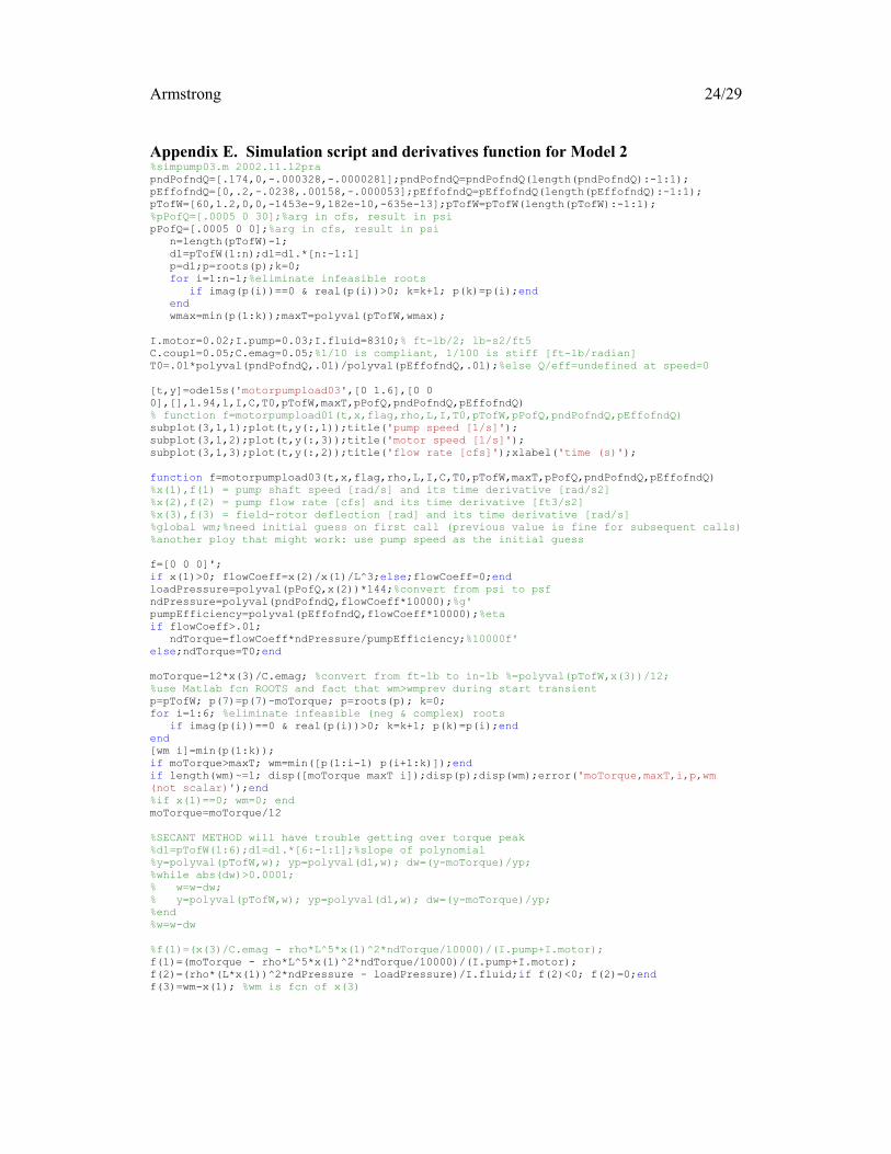
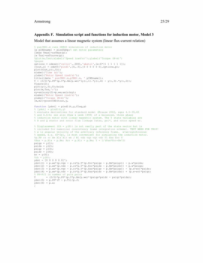
Appendix F. Simulation script and functions for induction motor, Model 3

Model that assumes a linear magnetic system (linear flux-current relation)

% punIND1.m runs ODE45 simulation of induction motor

[p pINDname] = pind3Qhp;% set motor parameters



%plot(w,Tss);xlabel('Speed (rad/s)');ylabel('Torque (N-m)')

%pause

options = odeset('reltol',.0001,'abstol',1e-6*[1 1 1 1 1 1]);

[tout,y] = ode45('pind1',[0,.5],[0 0 0 0 0 0],options,p);

plot(tout,y(:,5));

xlabel('Time (s)');

ylabel('Rotor Speed (rad/s)');

title([date ' punIND1.m,pIND1.m, ' pINDname]);

T = (3/2)*p.PP*(p.Y*p.Xm/p.we)*(y(:,1).*y(:,4) - y(:,3).*y(:,2));

figure(2);

plot(y(:,5),T);hold;

plot(w,Tss,'r');

xy=axis;xy(2)=p.we;axis(xy);

xlabel('Rotor Speed (rad/s)');

ylabel('Torque (N-m)');

[m,m2]=pconvIND(tout,y,

function [ydot] = pind1(t,y,flag,p)

% [ydot] = pind1(t,y)

% evaluate derivatives for standard model (Krause 2002, eqns 4.5-39,40

% and 4.6-6; see also Shaw & Leeb 1999) of a balanced, three phase

% induction motor with linear magnetic system. The 5 state variables are

% D and Q stator and rotor flux linkage rates, psi*, and rotor speed wr.

% Displacement (th = y(6)) is not really part of the state vector but is

% included for numerical consistency (same integration scheme). TEST NEED FOR THIS!

% w is angular velocity of the arbitrary reference frame. w=we=synchronous

% speed, e.g. 60*2pi, is most convenient for simulating the induction motor.

%p.PP rs rr Xm Xls Xlr we J Bl vds vqs vqr vdr Tl Xss Xrr Y

%Xss = p.Xls + p.Xm; Xrr = p.Xlr + p.Xm; Y = 1/(Xss*Xrr+Xm^2)

psiqs = y(1);

psids = y(2);

psiqr = y(3);

psidr = y(4);

wr = y(5);

%th = y(6);

ydot = [0 0 0 0 0 0]';

ydot(1) = p.we*(p.vqs - p.rs*p.Y*(p.Xrr*psiqs - p.Xm*psiqr)) - p.w*psids;

ydot(2) = p.we*(p.vds - p.rs*p.Y*(p.Xrr*psids - p.Xm*psidr)) + p.w*psiqs;

ydot(3) = p.we*(p.vqr - p.rr*p.Y*(p.Xss*psiqr - p.Xm*psiqs)) - (p.w-wr)*psidr;

ydot(4) = p.we*(p.vdr - p.rr*p.Y*(p.Xss*psidr - p.Xm*psids)) + (p.w-wr)*psiqr;

% PP=P/2 is number of pole pairs

T = (3/2)*p.PP*(p.Y*p.Xm/p.we)*(psiqs*psidr - psiqr*psids);

ydot(5) = p.PP*(T - p.Tl)/p.J;

ydot(6) = p.w;

;

Armstrong 26/29

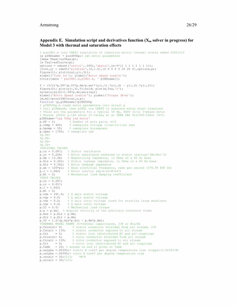
Appendix E. Simulation script and derivatives function (Xm solver in progress) for

Model 3 with thermal and saturation effects

% punIND1.m runs ODE45 simulation of induction motor; thermal states added 20021213

[p pINDname] = pind50hp;% set motor parameters



options = odeset('reltol',.0001,'abstol',1e-6*[1 1 1 1 1 1 1 1]);

[tout,y] = ode45('pind1sat',[0,1.4],[0 0 0 0 0 20 20 0],options,p);

figure(1); plot(tout,y(:,5));

xlabel('Time (s)'); ylabel('Rotor Speed (rad/s)');

title([date ' punIND1.m,pIND1.m, ' pINDname]);

T = (3/2)*p.PP*(p.YY*p.Xm/p.we)*(y(:,1).*y(:,4) - y(:,3).*y(:,2));

figure(2); plot(y(:,5),T);hold; plot(w,Tss,'r');

xy=axis;xy(2)=1.04*p.we;axis(xy);

xlabel('Rotor Speed (rad/s)'); ylabel('Torque (N-m)');

[m,m2]=pconvIND(tout,y,p);

function [p,pINDname]=pIND50hp

% pIND50hp.m loads motor parameters into struct p

% Call pINDparm, then pIND1 via ODE45 to simulate motor start transient

% These are the parameters for a typical 50 Hp, 480V (L-L) 3-phase motor

% Krause (2002) p.165 after JJ Cathay et al IEEE PAS 92(1399-1406) 1973.

pINDname='typ 50hp ind motor'

p.PP = 2; % Number of pole pairs =P/2

p.vnmp = 460; % nameplate voltage (line-to-line rms)

p.hpnmp = 50; % nameplate horsepower

p.rpmn = 1705; % nameplate rpm

%p.Vb=

%p.Pb=

%p.Tb=

%p.Ib=

%ORIGINAL VALUES

p.rs = 0.087; % Stator resistance

p.rr = 0.228; % Rotor resistance referred to stator (ractual*(Ns/Nr)^2)

p.Xm = 13.08; % Magnetizing impedance, in Ohms on a 60 Hz base

p.Xls = 0.302; % Stator leakage impedance, in Ohms on a 60 Hz base

p.Xlr = 0.302; % Rotor leakage impedance

p.we = 120*pi; % Base electrical frequency, rads per second (376.99 @60 Hz)

p.J = 1.662; % Rotor inertia (kg-m-s2=N-m3?)

p.Bl = 0; % Mechanical load damping coefficient

%TEST VALUES

p.rs = 0.087;

p.rr = 0.057;

p.J = 1.662;

p.Bl = 0;

p.vds = 391.9; % D axis stator voltage

p.vqs = 0.0; % Q axis stator voltage

p.vdr = 0.0; % D axis rotor voltage (used for starting large machines)

p.vqr = 0.0; % Q axis rotor voltage

p.Tl = 0.0; % Mechanical load torque

p.w = p.we; % Angular velocity of the arbitrary reference frame

p.Xss = p.Xls + p.Xm;

p.Xrr = p.Xlr + p.Xm;

p.YY = 1.0/(p.Xss*p.Xrr - p.Xm*p.Xm);

%THERMAL MODEL PARMS (C=thermal capacitance, J/K or Btu/R)

p.Cscslot= 0; % stator conductor shielded from air stream, J/K

p.Cscair = 130; % stator conductor exposed to air stream

p.Csi = 0; % stator iron (distributed RC and air coupling)

p.Crcslot= 0; % rotor conductor shielded from air stream

p.Crcair = 130; % rotor conductor exposed to air stream

p.Cri = 0; % rotor iron (distributed RC and air coupling)

p.Tamb = 20; % assume rs and rr given at Tamb

p.salpha =.00393;% stator R coeff per degree temperature rise (copper:0.00393/K)

p.ralpha =.00393;% rotor R coeff per degree temperature rise

p.uscair = 30;%123; %W/K

p.urcair = 30;%123;

Armstrong 27/29

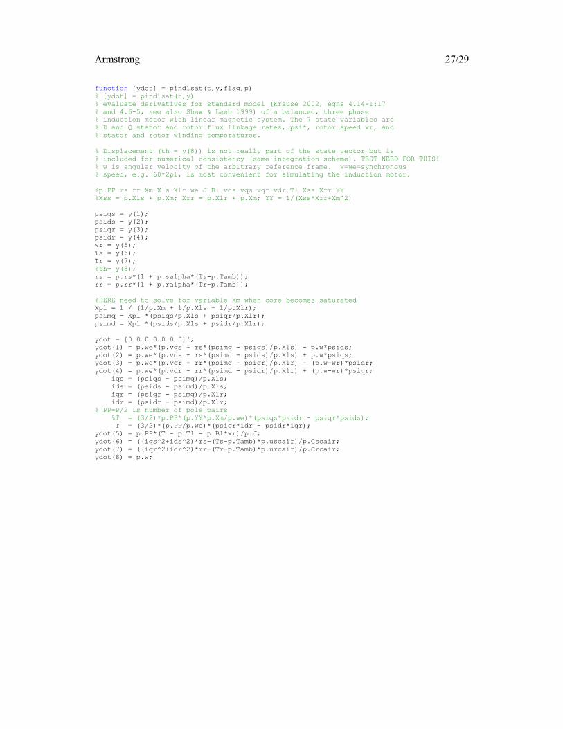
function [ydot] = pind1sat(t,y,flag,p)

% [ydot] = pind1sat(t,y)

% evaluate derivatives for standard model (Krause 2002, eqns 4.14-1:17


% induction motor with linear magnetic system. The 7 state variables are

% D and Q stator and rotor flux linkage rates, psi*, rotor speed wr, and

% stator and rotor winding temperatures.





%p.PP rs rr Xm Xls Xlr we J Bl vds vqs vqr vdr Tl Xss Xrr YY

%Xss = p.Xls + p.Xm; Xrr = p.Xlr + p.Xm; YY = 1/(Xss*Xrr+Xm^2)

psiqs = y(1);

psids = y(2);

psiqr = y(3);

psidr = y(4);

wr = y(5);

Ts = y(6);

Tr = y(7);

%th= y(8);

rs = p.rs*(1 + p.salpha*(Ts-p.Tamb));

rr = p.rr*(1 + p.ralpha*(Tr-p.Tamb));

%HERE need to solve for variable Xm when core becomes saturated

Xpl = 1 / (1/p.Xm + 1/p.Xls + 1/p.Xlr);

psimq = Xpl *(psiqs/p.Xls + psiqr/p.Xlr);

psimd = Xpl *(psids/p.Xls + psidr/p.Xlr);

ydot = [0 0 0 0 0 0 0]';

ydot(1) = p.we*(p.vqs + rs*(psimq - psiqs)/p.Xls) - p.w*psids;

ydot(2) = p.we*(p.vds + rs*(psimd - psids)/p.Xls) + p.w*psiqs;

ydot(3) = p.we*(p.vqr + rr*(psimq - psiqr)/p.Xlr) - (p.w-wr)*psidr;

ydot(4) = p.we*(p.vdr + rr*(psimd - psidr)/p.Xlr) + (p.w-wr)*psiqr;

iqs = (psiqs - psimq)/p.Xls;

ids = (psids - psimd)/p.Xls;

iqr = (psiqr - psimq)/p.Xlr;

idr = (psidr - psimd)/p.Xlr;


%T = (3/2)*p.PP*(p.YY*p.Xm/p.we)*(psiqs*psidr - psiqr*psids);

T = (3/2)*(p.PP/p.we)*(psiqr*idr - psidr*iqr);

ydot(5) = p.PP*(T - p.Tl - p.Bl*wr)/p.J;

ydot(6) = ((iqs^2+ids^2)*rs-(Ts-p.Tamb)*p.uscair)/p.Cscair;

ydot(7) = ((iqr^2+idr^2)*rr-(Tr-p.Tamb)*p.urcair)/p.Crcair;

ydot(8) = p.w;

Armstrong 28/29

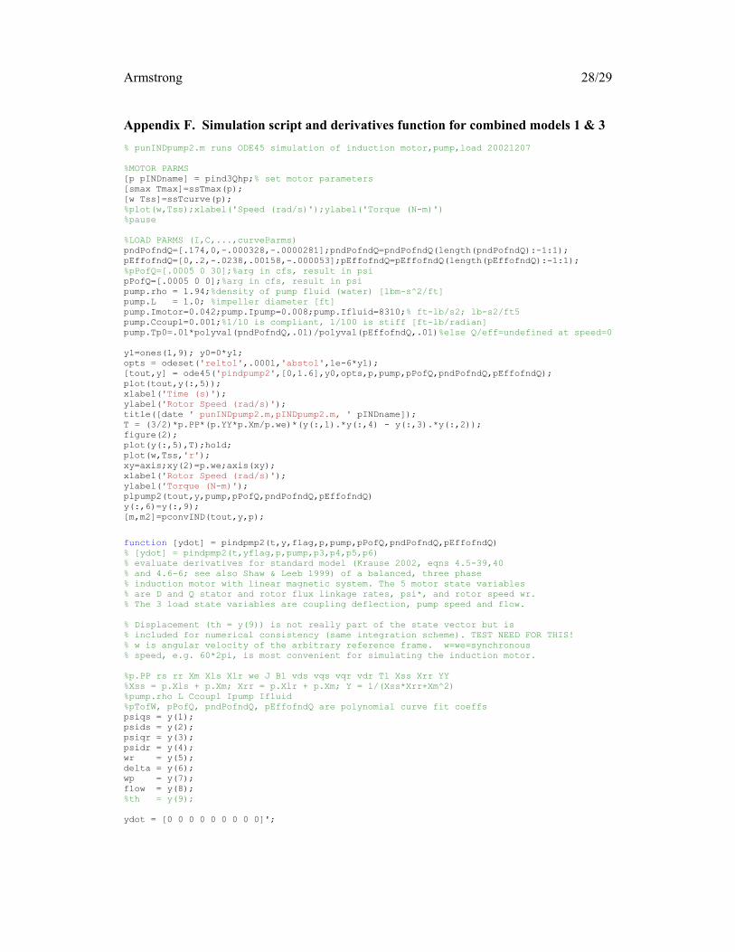
Appendix F. Simulation script and derivatives function for combined models 1 & 3

% punINDpump2.m runs ODE45 simulation of induction motor,pump,load 20021207

%MOTOR PARMS

[p pINDname] = pind3Qhp;% set motor parameters



%plot(w,Tss);xlabel('Speed (rad/s)');ylabel('Torque (N-m)')

%pause

%LOAD PARMS (I,C,...,curveParms)





pump.rho = 1.94;%density of pump fluid (water) [lbm-s^2/ft]

pump.L = 1.0; %impeller diameter [ft]

pump.Imotor=0.042;pump.Ipump=0.008;pump.Ifluid=8310;% ft-lb/s2; lb-s2/ft5

pump.Ccoupl=0.001;%1/10 is compliant, 1/100 is stiff [ft-lb/radian]

pump.Tp0=.01*polyval(pndPofndQ,.01)/polyval(pEffofndQ,.01)%else Q/eff=undefined at speed=0

y1=ones(1,9); y0=0*y1;

opts = odeset('reltol',.0001,'abstol',1e-6*y1);

[tout,y] = ode45('pindpump2',[0,1.6],y0,opts,p,pump,pPofQ,pndPofndQ,pEffofndQ);

plot(tout,y(:,5));

xlabel('Time (s)');

ylabel('Rotor Speed (rad/s)');

title([date ' punINDpump2.m,pINDpump2.m, ' pINDname]);

T = (3/2)*p.PP*(p.YY*p.Xm/p.we)*(y(:,1).*y(:,4) - y(:,3).*y(:,2));

figure(2);

plot(y(:,5),T);hold;

plot(w,Tss,'r');

xy=axis;xy(2)=p.we;axis(xy);

xlabel('Rotor Speed (rad/s)');

ylabel('Torque (N-m)');

plpump2(tout,y,pump,pPofQ,pndPofndQ,pEffofndQ)

y(:,6)=y(:,9);

[m,m2]=pconvIND(tout,y,p);

function [ydot] = pindpmp2(t,y,flag,p,pump,pPofQ,pndPofndQ,pEffofndQ)

% [ydot] = pindpmp2(t,yflag,p,pump,p3,p4,p5,p6)

% evaluate derivatives for standard model (Krause 2002, eqns 4.5-39,40


% induction motor with linear magnetic system. The 5 motor state variables

% are D and Q stator and rotor flux linkage rates, psi*, and rotor speed wr.

% The 3 load state variables are coupling deflection, pump speed and flow.





%p.PP rs rr Xm Xls Xlr we J Bl vds vqs vqr vdr Tl Xss Xrr YY

%Xss = p.Xls + p.Xm; Xrr = p.Xlr + p.Xm; Y = 1/(Xss*Xrr+Xm^2)

%pump.rho L Ccoupl Ipump Ifluid

%pTofW, pPofQ, pndPofndQ, pEffofndQ are polynomial curve fit coeffs

psiqs = y(1);

psids = y(2);

psiqr = y(3);

psidr = y(4);

wr = y(5);

delta = y(6);

wp = y(7);

flow = y(8);

%th = y(9);

ydot = [0 0 0 0 0 0 0 0 0]';

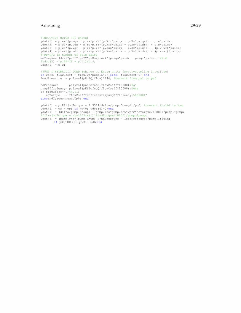
Armstrong 29/29

%INDUCTION MOTOR (SI units)

ydot(1) = p.we*(p.vqs - p.rs*p.YY*(p.Xrr*psiqs - p.Xm*psiqr)) - p.w*psids;

ydot(2) = p.we*(p.vds - p.rs*p.YY*(p.Xrr*psids - p.Xm*psidr)) + p.w*psiqs;

ydot(3) = p.we*(p.vqr - p.rr*p.YY*(p.Xss*psiqr - p.Xm*psiqs)) - (p.w-wr)*psidr;

ydot(4) = p.we*(p.vdr - p.rr*p.YY*(p.Xss*psidr - p.Xm*psids)) + (p.w-wr)*psiqr;


moTorque= (3/2)*p.PP*(p.YY*p.Xm/p.we)*(psiqs*psidr - psiqr*psids); %N-m

%ydot(5) = p.PP*(T - p.Tl)/p.J;

ydot(9) = p.w;

%PUMP & HYDRAULIC LOAD (change to Engrg units @motor-coupling interface)

if wp>0; flowCoeff = flow/wp/pump.L^3; else; flowCoeff=0; end

loadPressure = polyval(pPofQ,flow)*144; %convert from psi to psf

ndPressure = polyval(pndPofndQ,flowCoeff*10000);%g'

pumpEfficiency= polyval(pEffofndQ,flowCoeff*10000);%eta

if flowCoeff~=0;%>.01;

ndTorque = flowCoeff*ndPressure/pumpEfficiency;%10000f'

else;ndTorque=pump.Tp0; end

ydot(5) = p.PP*(moTorque - 1.3564*delta/pump.Ccoupl)/p.J; %convert ft-lbf to N-m

ydot(6) = wr - wp; if wp<0; ydot(6)=0;end

ydot(7) = (delta/pump.Ccoupl - pump.rho*pump.L^5*wp^2*ndTorque/10000)/pump.Ipump;

%f(1)=(moTorque - rho*L^5*x(1)^2*ndTorque/10000)/pump.Ipump;

ydot(8) = (pump.rho*(pump.L*wp)^2*ndPressure - loadPressure)/pump.Ifluid;

if ydot(8)<0; ydot(8)=0;end

pump fault detection and diagnosis (fdd) based on electrical … · pump fault detection and...

Documents