Purity Analysis:An Abstract Interpretation Formulation

Ravichandhran Madhavan, G. Ramalingam, and Kapil Vaswani

Microsoft Research, India.t-rakand,grama,kapilv@microsoft.com

Abstract. Salcianu and Rinard present a compositional purity analysisthat computes a summary for every procedure describing its side-effects.In this paper, we formalize a generalization of this analysis as an abstractinterpretation, present several optimizations and an empirical evaluationshowing the value of these optimizations. The Salcianu-Rinard analysismakes use of abstract heap graphs, similar to various heap analyses andcomputes a shape graph at every program point of an analyzed proce-dure. The key to our formalization is to view the shape graphs of theanalysis as an abstract state transformer rather than as a set of abstractstates: the concretization of a shape graph is a function that maps aconcrete state to a set of concrete states. The abstract interpretationformulation leads to a better understanding of the algorithm. More im-portantly, it makes it easier to change and extend the basic algorithm,while guaranteeing correctness, as illustrated by our optimizations.

1 Introduction

Compositional or modular analysis [6] is a key technique for scaling static anal-ysis to large programs. Our interest is in techniques that analyze a procedurein isolation, using pre-computed summaries for called procedures, computing asummary for the analyzed procedure. Such analyses are widely used and havebeen found to scale well. In this paper we consider an analysis presented bySalcianu and Rinard [17], based on a pointer analysis due to Whaley and Ri-nard [19], which we will refer to the WSR analysis. Though referred to as apurity analysis, it is a more general-purpose analysis that computes a summaryfor every procedure, in the presence of dynamic memory allocation, describingits side-effects. This is one of the few heap analyses that is capable of treatingprocedures in a compositional fashion.

WSR analysis is interesting for several reasons. Salcianu and Rinard presentan application of the analysis to classify a procedure as pure or impure, wherea procedure is impure if its execution can potentially modify pre-existing state.Increasingly, new language constructs (such as iterators, parallel looping con-structs and SQL-like query operators) are realized as higher-order library pro-cedures with procedural parameters that are expected to be side-effect free. Pu-rity checkers can serve as verification/bug-finding tools to check usage of theseconstructs. Our interest in this analysis stems from our use of an extension of

this analysis to statically verify the correctness of the use of speculative par-allelism [13]. WSR analysis can also help more sophisticated verification tools,such as [8], which use simpler analyses to identify procedure calls that do notaffect properties of interest to the verifier and can be abstracted away.

However, we felt the need for various extensions of the WSR analysis. A keymotivation was efficiency. Real-world applications make use of large librariessuch as the base class libraries in .NET. While the WSR analysis is reasonablyefficient, we find that it still does not scale to such libraries. Another motivationis increased functionality: our checker for speculative parallelism [13] needs someextra information (must-write sets) beyond that computed by the analysis. Afinal motivating factor is better precision: the WSR analysis declares “pure”procedures that use idioms like lazy initialization and caching as impure.

The desire for these extensions leads us to formulate, in this paper, the WSRanalysis as an abstract interpretation, to simplify reasoning about the soundnessof these extensions. The formulation of the WSR analysis as an abstract inter-pretation is, in fact, mentioned as an open problem by Salcianu ([16], page 128).

The WSR analysis makes use of abstract heap graphs, similar to various heapanalyses and computes a shape graph gu at every program point u of an ana-lyzed procedure. The key to our abstract interpretation formulation, however, isto view a shape graph utilized by the analysis as an abstract state transformerrather than as a set of abstract states: thus, the concretization of a shape graphis a function that maps a concrete state to a set of concrete states. Specifically,if the graph computed at program point u is gu, then for any concrete state σ,γ(gu)(σ) conservatively approximates the set of states that can arise at programpoint u in the execution of the procedure on an initial state σ. In our formal-ization, we present a concrete semantics in the style of the functional approachto interprocedural analysis presented by Sharir and Pnueli. The WSR analysiscan then be seen as a natural abstract interpretation of this concrete semantics.

We then present three optimizations viz. duplicate node merging, summarymerging, and safe node elimination, that improve the efficiency of WSR analysis.We use the abstract interpretation formulation to show that these optimizationsare sound. Our experiments show that these optimizations significantly reduceboth analysis time (sometimes by two orders of magnitude or more) and memoryconsumption, allowing the analysis to scale to large programs.

2 The Language, Concrete Semantics, And The Problem

Syntax A program consists of a set of procedures. A procedure P consists ofa control-flow graph, with an entry vertex entry(P ) and an exit vertex exit(P ).The entry vertex has no predecessor and the exit vertex has no successor. Everyedge of the control-flow graph is labelled by a primitive statement. The set of

primitive statements are shown in Fig. 1. We use uS→ v to indicate an edge in

the control-flow graph from vertex u to vertex v labelled by statement S.Concrete Semantics Domain Let Vars denote the set of variable names

used in the program, partitioned into the following disjoint sets: the set of global

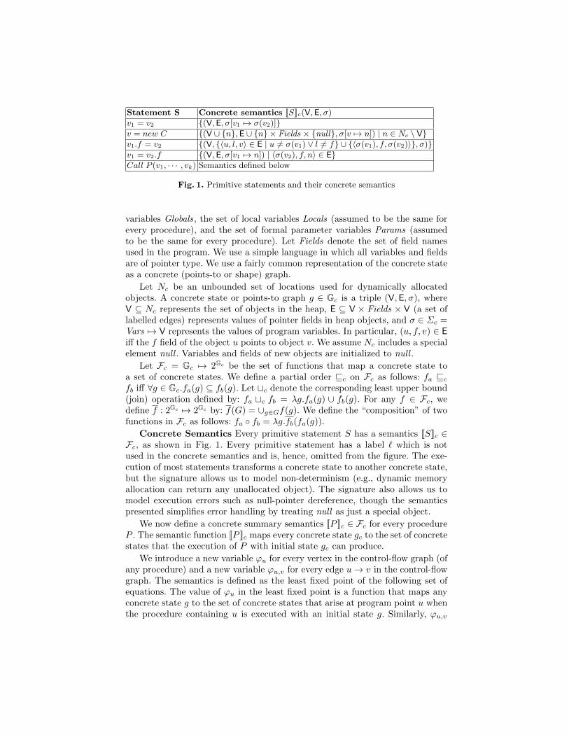
Statement S Concrete semantics [[S]]c(V,E, σ)

v1 = v2 {(V,E, σ[v1 7→ σ(v2)]}v = new C {(V ∪ {n},E ∪ {n} × Fields × {null}, σ[v 7→ n]) | n ∈ Nc \ V}v1.f = v2 {(V, {〈u, l, v〉 ∈ E | u 6= σ(v1) ∨ l 6= f} ∪ {〈σ(v1), f, σ(v2)〉}, σ)}v1 = v2.f {(V,E, σ[v1 7→ n]) | 〈σ(v2), f, n〉 ∈ E}Call P (v1, · · · , vk) Semantics defined below

Fig. 1. Primitive statements and their concrete semantics

variables Globals, the set of local variables Locals (assumed to be the same forevery procedure), and the set of formal parameter variables Params (assumedto be the same for every procedure). Let Fields denote the set of field namesused in the program. We use a simple language in which all variables and fieldsare of pointer type. We use a fairly common representation of the concrete stateas a concrete (points-to or shape) graph.

Let Nc be an unbounded set of locations used for dynamically allocatedobjects. A concrete state or points-to graph g ∈ Gc is a triple (V,E, σ), whereV ⊆ Nc represents the set of objects in the heap, E ⊆ V × Fields × V (a set oflabelled edges) represents values of pointer fields in heap objects, and σ ∈ Σc =Vars 7→ V represents the values of program variables. In particular, (u, f, v) ∈ Eiff the f field of the object u points to object v. We assume Nc includes a specialelement null . Variables and fields of new objects are initialized to null .

Let Fc = Gc 7→ 2Gc be the set of functions that map a concrete state toa set of concrete states. We define a partial order vc on Fc as follows: fa vcfb iff ∀g ∈ Gc.fa(g) ⊆ fb(g). Let tc denote the corresponding least upper bound(join) operation defined by: fa tc fb = λg.fa(g) ∪ fb(g). For any f ∈ Fc, wedefine f : 2Gc 7→ 2Gc by: f(G) = ∪g∈Gf(g). We define the “composition” of twofunctions in Fc as follows: fa ◦ fb = λg.fb(fa(g)).

Concrete Semantics Every primitive statement S has a semantics [[S]]c ∈Fc, as shown in Fig. 1. Every primitive statement has a label ` which is notused in the concrete semantics and is, hence, omitted from the figure. The exe-cution of most statements transforms a concrete state to another concrete state,but the signature allows us to model non-determinism (e.g., dynamic memoryallocation can return any unallocated object). The signature also allows us tomodel execution errors such as null-pointer dereference, though the semanticspresented simplifies error handling by treating null as just a special object.

We now define a concrete summary semantics [[P ]]c ∈ Fc for every procedureP . The semantic function [[P ]]c maps every concrete state gc to the set of concretestates that the execution of P with initial state gc can produce.

We introduce a new variable ϕu for every vertex in the control-flow graph (ofany procedure) and a new variable ϕu,v for every edge u→ v in the control-flowgraph. The semantics is defined as the least fixed point of the following set ofequations. The value of ϕu in the least fixed point is a function that maps anyconcrete state g to the set of concrete states that arise at program point u whenthe procedure containing u is executed with an initial state g. Similarly, ϕu,v

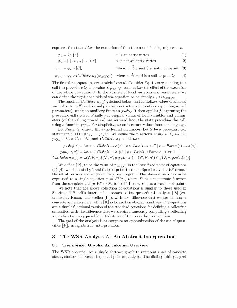
captures the states after the execution of the statement labelling edge u→ v.

ϕv = λg.{g} v is an entry vertex (1)

ϕv =⊔c{ϕu,v | u→ v} v is not an entry vertex (2)

ϕu,v = ϕu ◦ [[S]]c where uS→ v and S is not a call-stmt (3)

ϕu,v = ϕu ◦ CallReturnS(ϕexit(Q)) where uS→ v, S is a call to proc Q (4)

The first three equations are straightforward. Consider Eq. 4, corresponding to acall to a procedure Q. The value of ϕexit(Q) summarizes the effect of the executionof the whole procedure Q. In the absence of local variables and parameters, wecan define the right-hand-side of the equation to be simply ϕu ◦ ϕexit(Q).

The function CallReturnS(f), defined below, first initializes values of all localvariables (to null) and formal parameters (to the values of corresponding actualparameters), using an auxiliary function pushS . It then applies f , capturing theprocedure call’s effect. Finally, the original values of local variables and param-eters (of the calling procedure) are restored from the state preceding the call,using a function popS . For simplicity, we omit return values from our language.

Let Param(i) denote the i-the formal parameter. Let S be a procedure callstatement “Call Q(a1,...,ak)”. We define the functions pushS ∈ Σc 7→ Σc,popS ∈ Σc ×Σc 7→ Σc, and CallReturnS as follows:

pushS(σ) = λv. v ∈ Globals → σ(v) | v ∈ Locals → null | v = Param(i)→ σ(ai)

popS(σ, σ′) = λv. v ∈ Globals → σ′(v) | v ∈ Locals ∪ Params → σ(v)

CallReturnS(f) = λ(V,E, σ).{(V′,E′, popS(σ, σ′)) | (V′,E′, σ′) ∈ f(V,E, pushS(σ))}

We define [[P ]]c to be the value of ϕexit(P ) in the least fixed point of equations(1)-(4), which exists by Tarski’s fixed point theorem. Specifically, let VE denotethe set of vertices and edges in the given program. The above equations can beexpressed as a single equation ϕ = F \(ϕ), where F \ is a monotonic functionfrom the complete lattice VE 7→ Fc to itself. Hence, F \ has a least fixed point.

We note that the above collection of equations is similar to those used inSharir and Pnueli’s functional approach to interprocedural analysis [18] (ex-tended by Knoop and Steffen [10]), with the difference that we are defining aconcrete semantics here, while [18] is focused on abstract analyses. The equationsare a simple functional version of the standard equations for defining a collectingsemantics, with the difference that we are simultaneously computing a collectingsemantics for every possible initial states of the procedure’s execution.

The goal of the analysis is to compute an approximation of the set of quan-tities [[P ]]c using abstract interpretation.

3 The WSR Analysis As An Abstract Interpretation

3.1 Transformer Graphs: An Informal Overview

The WSR analysis uses a single abstract graph to represent a set of concretestates, similar to several shape and pointer analyses. The distinguishing aspect

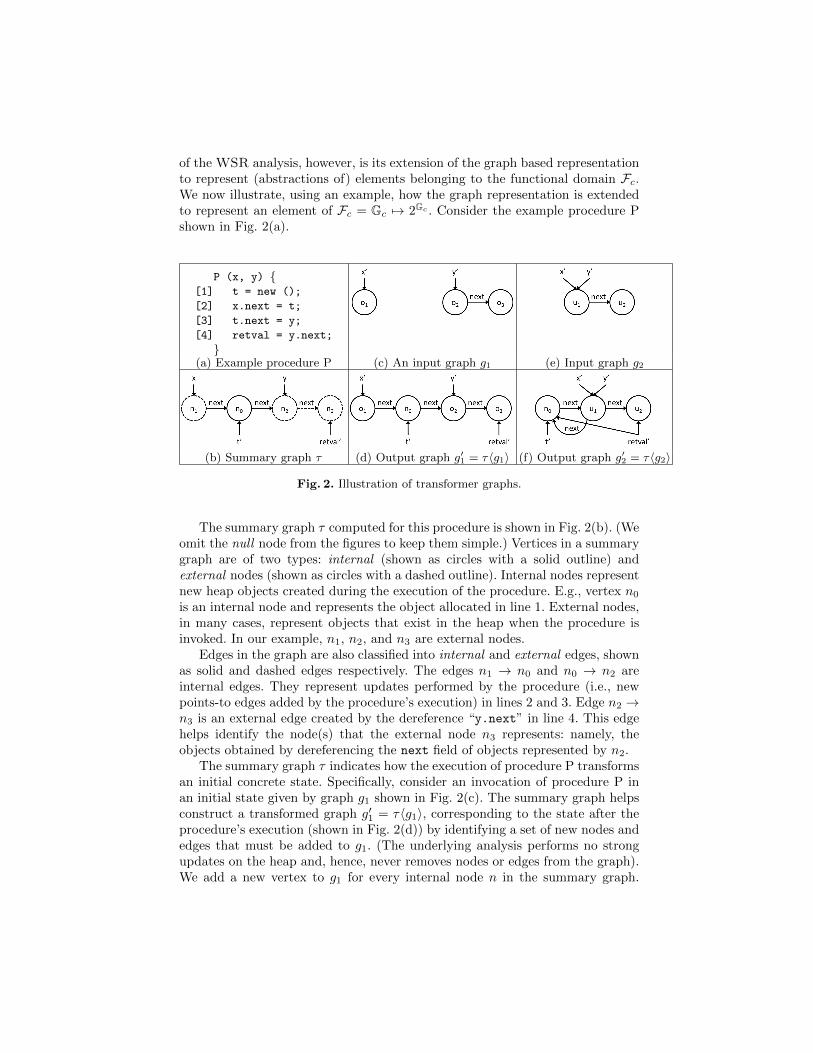
of the WSR analysis, however, is its extension of the graph based representationto represent (abstractions of) elements belonging to the functional domain Fc.We now illustrate, using an example, how the graph representation is extendedto represent an element of Fc = Gc 7→ 2Gc . Consider the example procedure Pshown in Fig. 2(a).

P (x, y) {[1] t = new ();

[2] x.next = t;

[3] t.next = y;

[4] retval = y.next;

}(a) Example procedure P (c) An input graph g1 (e) Input graph g2

(b) Summary graph τ (d) Output graph g′1 = τ〈g1〉 (f) Output graph g′2 = τ〈g2〉

Fig. 2. Illustration of transformer graphs.

The summary graph τ computed for this procedure is shown in Fig. 2(b). (Weomit the null node from the figures to keep them simple.) Vertices in a summarygraph are of two types: internal (shown as circles with a solid outline) andexternal nodes (shown as circles with a dashed outline). Internal nodes representnew heap objects created during the execution of the procedure. E.g., vertex n0is an internal node and represents the object allocated in line 1. External nodes,in many cases, represent objects that exist in the heap when the procedure isinvoked. In our example, n1, n2, and n3 are external nodes.

Edges in the graph are also classified into internal and external edges, shownas solid and dashed edges respectively. The edges n1 → n0 and n0 → n2 areinternal edges. They represent updates performed by the procedure (i.e., newpoints-to edges added by the procedure’s execution) in lines 2 and 3. Edge n2 →n3 is an external edge created by the dereference “y.next” in line 4. This edgehelps identify the node(s) that the external node n3 represents: namely, theobjects obtained by dereferencing the next field of objects represented by n2.

The summary graph τ indicates how the execution of procedure P transformsan initial concrete state. Specifically, consider an invocation of procedure P inan initial state given by graph g1 shown in Fig. 2(c). The summary graph helpsconstruct a transformed graph g′1 = τ〈g1〉, corresponding to the state after theprocedure’s execution (shown in Fig. 2(d)) by identifying a set of new nodes andedges that must be added to g1. (The underlying analysis performs no strongupdates on the heap and, hence, never removes nodes or edges from the graph).We add a new vertex to g1 for every internal node n in the summary graph.

Every external node n in the summary graph represents a set of vertices η(n) ing′1. (We will explain later how the function η is determined by τ .) Every internal

edge uh→ v in the summary graph identifies a set of edges {u′ h→ v′ | u′ ∈

η(u), v′ ∈ η(v)} that must be added to the graph g′1. In our example, n1, n2 andn3 represent, respectively, {o1}, {o2} and {o3}. This produces the graph shownin Fig. 2(d), which is an abstract graph representing a set of concrete states. Theprimed variables in the summary graph represent the (final) values of variables,and are used to determine the values of variables in the output graph.

An important aspect of the summary computed by the WSR analysis is thatit can be used even in the presence of potential aliases in the input (or cut-points [14]). Consider the input state g2 shown in Fig. 2(e), in which parametersx and y point to the same object u1. Our earlier description of how to constructthe output graph still applies in this context. The main tricky aspect here is incorrectly dealing with aliasing in the input. In the concrete execution, the updateto x.next in line 2 updates the next field of object u1. The aliasing between x

and y means that y.next will evaluate to n0 in line 4. Thus, in the concrete exe-cution retval will point to the newly created object n0 at the end of procedureexecution, rather than u2. This complication is dealt with in the definition ofthe mapping function η. For the example input g2, the external node n3 of thesummary graph represents the set of nodes {u2, n0}. (This is an imprecise, butsound, treatment of the aliasing situation.) The rest of the construction appliesjust as before. This yields the abstract graph shown in Fig. 2(f).

More generally, an external node in the summary graph acts as a proxy fora set of vertices in the final output graph to be constructed, which may includenodes that exist in the input graph as well as new nodes added to the inputgraph (which themselves correspond to internal nodes of the summary graph).

We now define the transformer graph domain formally.

3.2 The Abstract Domain

The Abstract Graph Domain We utilize a fairly standard abstract shape(or points-to) graph to represent a set of concrete states. Our formulation isparameterized by a given set Na, the universal set of all abstract graph nodes.An abstract shape graph g ∈ Ga is a triple (V,E, σ), where V ⊆ Na representsthe set of abstract heap objects, E ⊆ V × Fields × V (a set of labelled edges)represents possible values of pointer fields in the abstract heap objects, andσ ∈ Vars 7→ 2V is a map representing the possible values of program variables.

Given a concrete graph g1 = 〈V1,E1, σ1〉 and an abstract graph g2 = 〈V2,E2, σ2〉we say that g1 can be embedded into g2, denoted g1 � g2, if there exists afunction h : V1 7→ V2 such that 〈x, f, y〉 ∈ E1 ⇒ 〈h(x), f, h(y)〉 ∈ E2 and∀v ∈ Vars. σ2(v) ⊇ {h(σ1(v))}. The concretization γG(ga) of an abstract graphga is defined to be the set of all concrete graphs that can be embedded into ga:

γG(ga) = {gc ∈ Gc | gc � ga}

The Abstract Functional Domain. We now define the domain of graphsused to represent summary functions. A transformer graph τ ∈ Fa is a tuple

(EV,EE, π, IV, IE, σ), where EV ⊆ Na is the set of external vertices, IV ⊆ Nais the set of internal vertices, EE ⊆ V × Fields × V is the set of externaledges, where V = EV ∪ IV, IE ⊆ V × Fields × V is the set of internal edges,π ∈ (Params ∪Globals) 7→ 2V is a map representing the values of parametersand global variables in the initial state, and σ ∈ Vars 7→ 2V is a map representingthe possible values of program variables in the transformed state. Furthermore,a transformer graph τ is required to satisfy the following constraints:

〈x, f, y〉 ∈ EE =⇒ ∃u ∈ range(π).x is reachable from u via (IE ∪ EE) edges

y ∈ EV =⇒ y ∈ range(π) ∨ ∃〈x, f, y〉 ∈ EE

Given a transformer graph τ = (EV,EE, π, IV, IE, σ), a node u is said to be aparameter node if u ∈ range(π). A node u is said to be an escaping node if itis reachable from some parameter node via a path of zero or more edges (eitherinternal or external). Let Escaping(τ) denote the set of escaping nodes in τ .

We now define the concretization function γT : Fa → Fc. Given a transformergraph τ = (EV,EE, π, IV, IE, σ) and a concrete graph gc = (Vc,Ec, σc), we needto construct a graph representing the transformation of gc by τ . As explainedearlier, every external node n ∈ EV in the transformer graph represents a setof vertices in the transformed graph. We now define a function η : (IV ∪ EV) 7→2(IV∪Vc) that maps each node in the transformer graph to a set of concrete nodes(in gc) as well as internal nodes (in τ) as the least solution to the following setof constraints over variable µ.

v ∈ IV⇒ v ∈ µ(v) (5)

v ∈ π(X)⇒ σc(X) ∈ µ(v) (6)

〈u, f, v〉 ∈ EE, u′ ∈ µ(u), 〈u′, f, v′〉 ∈ Ec ⇒ v′ ∈ µ(v) (7)

〈u, f, v〉 ∈ EE, µ(u) ∩ µ(u′) 6= ∅, 〈u′, f, v′〉 ∈ IE⇒ µ(v′) ⊆ µ(v) (8)

Explanation of the constraints: An internal node represents itself (Eq. 5). Anexternal node labelled by a parameter X represents the node pointed to by X inthe input state gc (Eq. 6). An external edge 〈u, f, v〉 indicates that v representsany f -successor v′ of any node u′ represented by u in the input state (Eq. 7).However, with an external edge 〈u, f, v〉, we must also account for updates tothe f field of the objects represented by u during the procedure execution, ie,the transformation represented by τ , via aliases (as illustrated by the examplein Fig. 2(e)). Eq. 8 handles this. The precondition identifies u′ as a potentialalias for u (for the given input graph), and identifies updates performed on thef field of (nodes represented by) u′.

Given mapping function η, we define the transformed abstract graph τ〈gc〉 as〈V′,E′, σ′〉, where V′ = Vc∪IV, E′ = Ec∪{〈v1, f, v2〉 | 〈u, f, v〉 ∈ IE, v1 ∈ η(u), v2 ∈η(v)} and σ′ = λx.

⋃u∈σ(x) η(u). The transformed graph is an abstract graph

that represents all concrete graphs that can be embedded in the abstract graph.Thus, we define the concretization function as below:

γT (τa) = λgc.γG(τa〈gc〉).

Our abstract interpretation formulation uses only a concretization function.There is no abstraction function αT . While this form is less common, it is suffi-cient to establish the soundness of the analysis, as explained in [5]. Specifically,a concrete value f ∈ Fc is correctly represented by an abstract value τ ∈ Fa, de-noted f ∼ τ , iff f vc γT (τ). We seek to compute an abstract value that correctlyrepresents the least fixed point of the concrete semantic equations.

Containment Ordering. A natural “precision ordering” exists on Fa, whereτ1 is said to be more precise than τ2 iff γT (τ1) vc γT (τ2). However, this ordering isnot of immediate interest to us. (It is not even a partial order, and is hard to workwith computationally.) We utilize a stricter ordering in our abstract fixed pointcomputation. We define a relation vco on Fa by: (EV1,EE1, π1, IV1, IE1, σ1) vco(EV2,EE2, π2, IV2, IE2, σ2) iff EV1 ⊆ EV2, EE1 ⊆ EE2, ∀x.π1(x) ⊆ π2(x), IV1 ⊆IV2, IE1 ⊆ IE2, and ∀x.σ1(x) ⊆ σ2(x).

Lemma 1. vco is a partial-order on Fa with a join operation, denoted tco.Further, γT is monotonic with respect to vco: τ1 vco τ2 ⇒ γT (τ1) vc γT (τ2).

3.3 The Abstract Semantics

Our goal is to approximate the least fixed point computation of the concretesemantics equations 1-4. We do this by utilizing an analogous set of abstractsemantics equations shown below. First, we fix the set Na of abstract nodes.Recall that the domain Fa defined earlier is parameterized by this set. The WSRalgorithm relies on an “allocation site” based merging strategy for bounding thesize of the transformer graphs. We utilize the labels attached to statements asallocation-site identifiers. Let Labels denote the set of statement labels in thegiven program. We define Na to be {nx | x ∈ Labels ∪ Params ∪Globals}.

We first introduce a variable ϑu for every vertex u in the control-flow graph(denoting the abstract value at a program point u), and a variable ϑu,v for everyedge u → v in the control-flow graph (denoting the abstract value after theexecution of the statement in edge u→ v).

ϑv = ID v is an entry vertex (9)

ϑv = tco{ϑu,v | uS→ v} v is not an entry vertex (10)

ϑu,v = [[S]]a(ϑu) where uS→ v,S is not a call-stmt (11)

ϑu,v = ϑexit(Q)〈〈ϑu〉〉Sa where uS→ v,S is a call to Q (12)

Here, ID is a transformer graph consisting of a external vertex for each globalvariable and each parameter (representing the identity function). Formally, ID =(EV, ∅, π, ∅, ∅, π), where EV = {nx | x ∈ Params ∪ Globals} and π = λv. v ∈Params ∪ Globals → nv | v ∈ Locals → null . The abstract semantics [[S]]a ofany primitive statement S, other than a procedure call, is shown in Figure 3.The abstract semantics of a procedure call is captured by an operator τ1〈〈τ2〉〉Sa ,which we will define soon.

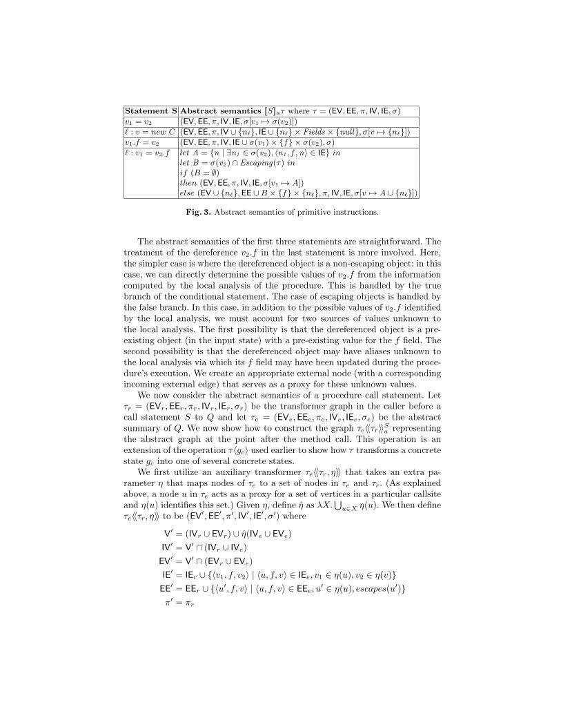
Statement S Abstract semantics [[S]]aτ where τ = (EV,EE, π, IV, IE, σ)

v1 = v2 (EV,EE, π, IV, IE, σ[v1 7→ σ(v2)])

` : v = new C (EV,EE, π, IV ∪ {n`}, IE ∪ {n`} × Fields × {null}, σ[v 7→ {n`}])v1.f = v2 (EV,EE, π, IV, IE ∪ σ(v1)× {f} × σ(v2), σ)

` : v1 = v2.f let A = {n | ∃n1 ∈ σ(v2 ), 〈n1 , f ,n〉 ∈ IE} inlet B = σ(v2 ) ∩ Escaping(τ) inif (B = ∅)then (EV,EE, π, IV, IE, σ[v1 7→ A])else (EV ∪ {n`},EE ∪B × {f} × {n`}, π, IV, IE, σ[v 7→ A ∪ {n`}])

Fig. 3. Abstract semantics of primitive instructions.

The abstract semantics of the first three statements are straightforward. Thetreatment of the dereference v2.f in the last statement is more involved. Here,the simpler case is where the dereferenced object is a non-escaping object: in thiscase, we can directly determine the possible values of v2.f from the informationcomputed by the local analysis of the procedure. This is handled by the truebranch of the conditional statement. The case of escaping objects is handled bythe false branch. In this case, in addition to the possible values of v2.f identifiedby the local analysis, we must account for two sources of values unknown tothe local analysis. The first possibility is that the dereferenced object is a pre-existing object (in the input state) with a pre-existing value for the f field. Thesecond possibility is that the dereferenced object may have aliases unknown tothe local analysis via which its f field may have been updated during the proce-dure’s execution. We create an appropriate external node (with a correspondingincoming external edge) that serves as a proxy for these unknown values.

We now consider the abstract semantics of a procedure call statement. Letτr = (EVr,EEr, πr, IVr, IEr, σr) be the transformer graph in the caller before acall statement S to Q and let τe = (EVe,EEe, πe, IVe, IEe, σe) be the abstractsummary of Q. We now show how to construct the graph τe〈〈τr〉〉Sa representingthe abstract graph at the point after the method call. This operation is anextension of the operation τ〈gc〉 used earlier to show how τ transforms a concretestate gc into one of several concrete states.

We first utilize an auxiliary transformer τe〈〈τr, η〉〉 that takes an extra pa-rameter η that maps nodes of τe to a set of nodes in τe and τr. (As explainedabove, a node u in τe acts as a proxy for a set of vertices in a particular callsiteand η(u) identifies this set.) Given η, define η as λX.

⋃u∈X η(u). We then define

τe〈〈τr, η〉〉 to be (EV′,EE′, π′, IV′, IE′, σ′) where

V′ = (IVr ∪ EVr) ∪ η(IVe ∪ EVe)

IV′ = V′ ∩ (IVr ∪ IVe)

EV′ = V′ ∩ (EVr ∪ EVe)

IE′ = IEr ∪ {〈v1, f, v2〉 | 〈u, f, v〉 ∈ IEe, v1 ∈ η(u), v2 ∈ η(v)}EE′ = EEr ∪ {〈u′, f, v〉 | 〈u, f, v〉 ∈ EEe, u

′ ∈ η(u), escapes(u′)}π′ = πr

σ′ = λx. x ∈ Globals → η(σe(x)) | x ∈ Locals ∪ Params → σr(x)

escapes(v) ≡ ∃u ∈ range(π′).v is reachable from u via IE′ ∪ EE′ edges

The predicate “escapes(u′)” used in the above definition is recursively dependenton the graph τ ′ being constructed: it checks if u′ is reachable from any of theparameter nodes in the graph being constructed. Thus, this leads to an iterativeprocess for adding edges to the graph being constructed, as more escaping nodesare identified.

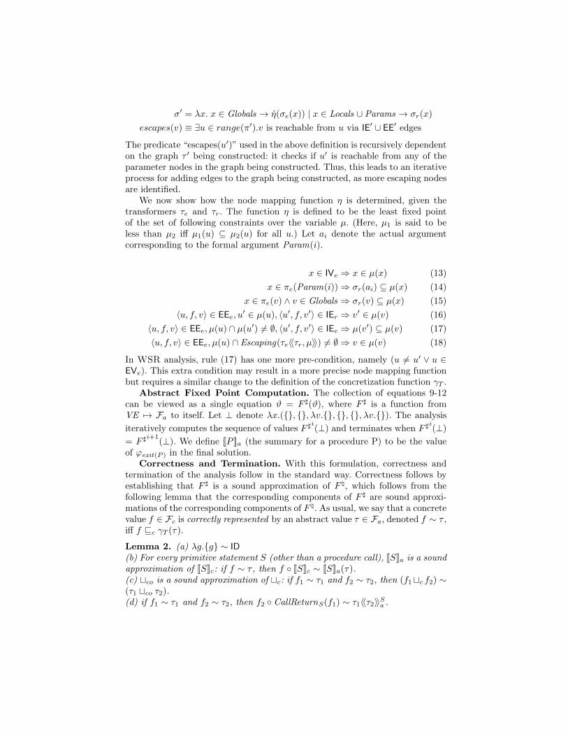
We now show how the node mapping function η is determined, given thetransformers τe and τr. The function η is defined to be the least fixed pointof the set of following constraints over the variable µ. (Here, µ1 is said to beless than µ2 iff µ1(u) ⊆ µ2(u) for all u.) Let ai denote the actual argumentcorresponding to the formal argument Param(i).

x ∈ IVe ⇒ x ∈ µ(x) (13)

x ∈ πe(Param(i))⇒ σr(ai) ⊆ µ(x) (14)

x ∈ πe(v) ∧ v ∈ Globals ⇒ σr(v) ⊆ µ(x) (15)

〈u, f, v〉 ∈ EEe, u′ ∈ µ(u), 〈u′, f, v′〉 ∈ IEr ⇒ v′ ∈ µ(v) (16)

〈u, f, v〉 ∈ EEe, µ(u) ∩ µ(u′) 6= ∅, 〈u′, f, v′〉 ∈ IEe ⇒ µ(v′) ⊆ µ(v) (17)

〈u, f, v〉 ∈ EEe, µ(u) ∩ Escaping(τe〈〈τr, µ〉〉) 6= ∅ ⇒ v ∈ µ(v) (18)

In WSR analysis, rule (17) has one more pre-condition, namely (u 6= u′ ∨ u ∈EVe). This extra condition may result in a more precise node mapping functionbut requires a similar change to the definition of the concretization function γT .

Abstract Fixed Point Computation. The collection of equations 9-12can be viewed as a single equation ϑ = F ](ϑ), where F ] is a function fromVE 7→ Fa to itself. Let ⊥ denote λx.({}, {}, λv.{}, {}, {}, λv.{}). The analysis

iteratively computes the sequence of values F ]i(⊥) and terminates when F ]

i(⊥)

= F ]i+1

(⊥). We define [[P ]]a (the summary for a procedure P) to be the valueof ϕexit(P ) in the final solution.

Correctness and Termination. With this formulation, correctness andtermination of the analysis follow in the standard way. Correctness follows byestablishing that F ] is a sound approximation of F \, which follows from thefollowing lemma that the corresponding components of F ] are sound approxi-mations of the corresponding components of F \. As usual, we say that a concretevalue f ∈ Fc is correctly represented by an abstract value τ ∈ Fa, denoted f ∼ τ ,iff f vc γT (τ).

Lemma 2. (a) λg.{g} ∼ ID(b) For every primitive statement S (other than a procedure call), [[S]]a is a soundapproximation of [[S]]c: if f ∼ τ , then f ◦ [[S]]c ∼ [[S]]a(τ).(c) tco is a sound approximation of tc: if f1 ∼ τ1 and f2 ∼ τ2, then (f1tc f2) ∼(τ1 tco τ2).(d) if f1 ∼ τ1 and f2 ∼ τ2, then f2 ◦ CallReturnS(f1) ∼ τ1〈〈τ2〉〉Sa .

Lemma 2 implies the following soundness theorem in the standard way (e.g., seeProposition 4.3 of [5]).

Theorem 1. The computed procedure summaries are correct. (For every proce-dure P, [[P ]]c ∼ [[P ]]a.)

Termination follows by establishing that F ] is monotonic with respect tov∗co, since Fa has only finite height vco-chains. Proofs of all results appear in[11].

4 Optimizations

We have implemented the WSR analysis for .NET binaries. More details aboutthe implementation and how we deal with language features absent in the corelanguage used in our formalization appear in [11]. In this section we describethree optimizations for the analysis that were motivated by our implementationexperience. We do not describe optimizations already discussed by WSR in [19]and [17]. We present an empirical evaluation of the impact of these optimizationson the scalability and the precision of the purity analysis in the experimentalevaluation section.

Optimization 1: Node Merging. Informally, we define node merging asan operation that replaces a set of nodes {n1, n2 . . . nm} by a single node nrepsuch that any predecessor or successor of the nodes n1, n2, . . . , nm becomes,respectively, a predecessor or successor of nrep. While merging nodes seems likea natural heuristic for improving efficiency, it does introduce some subtle issuesand challenges. The intuition for merging nodes arises from their use in thecontext of heap analyses where graphs represent sets of concrete states. However,in our context, graphs represent state transformers. We now present some resultsthat help establish the correctness of this optimization.

We now extend the notion of graph embedding to transformer graphs. Givenτ1 = (EV1,EE1, π1, IV1, IE1, σ1) and τ2 = (EV2,EE2, π2, IV2, IE2, σ2), we say thatτ1 � τ2 iff there exists a function h : (IV1∪EV1) 7→ (IV2∪EV2) such that: for everyinternal (respectively, external) node x in τ1 , h(x) is an internal (respectively,external) node; for every internal (respectively, external) edge 〈x, f, y〉 in τ1,〈h(x), f, h(y)〉 is an internal (respectively, external) edge in τ2, for every variable

x, h(σ1(x)) ⊆ σ2(x) and h(π1(x)) ⊆ π2(x) where h(Z) = {h(u) | u ∈ Z}.Node merging produces an embedding. Assume that we are given an equiv-

alence relation ' on the nodes of a transformer graph τ (such that no internalnodes are equivalent to external nodes). We define the transformer graph τ/ 'to be the transformer graph obtained by replacing every node u by a uniquerepresentative of its '-equivalence class in every component of τ .

Lemma 3. (a) � is a pre-order. (b) γT is monotonic with respect to �: i.e.,∀τa, τb ∈ Fa.τa � τb ⇒ γT (τa) vc γT (τb). (c) τ � (τ/ ').

Assume that we wish to replace a transformer graph τ by a graph τ/ ' atsome point during the analysis (perhaps by incorporating this into one of the

abstract operations). Our earlier correctness argument still remains valid (sinceif f ∼ τ1 � τ2, then f ∼ τ2).

However, this optimization impacts the termination argument because we donot have τ vco (τ/ '). Indeed, our initial implementation of the optimizationdid not terminate for one program because the computation ended up with acycle of equivalent, but different, transformers (in the sense of having the sameconcretization). Refining the implementation to ensure that once two nodes arechosen to be merged together, they are always merged together in all subsequentsteps, guarantees termination. Technically, we enhance the domain to include anequivalence relation on nodes (representing the nodes currently merged together)and update the transformers accordingly. A suitably modified ordering relationensures termination. Details are omitted due to space constraints, but this illus-trated to us the value of the abstract interpretation formalism (see [11] for moredetails).

The main advantage of the node merging optimization is that it reduces thesize of the transformer graph while every other transfer function increases thesize of the transformer graphs. However, when used injudiciously, node mergingcan result in loss of precision. In our implementation we use a couple of heuristicsto identify the set of nodes to be merged.

Given τ ∈ Fa and v1, v2 ∈ V(τ), we merge v1, v2 iff one of the two conditionshold (a) v1, v2 ∈ EV(τ) and ∃u ∈ V(τ) s.t. 〈u, f, v1〉 ∈ EE(τ) and 〈u, f, v2〉 ∈EE(τ) for some field f or (b) v1, v2 ∈ IV(τ) and ∃u ∈ V(τ) s.t. 〈u, f, v1〉 ∈ IE(τ)and 〈u, f, v2〉 ∈ IE(τ) for some field f .

In the WSR analysis, an external edge 〈u, f, v〉 on an escaping node u isoften used to identify objects that u.f may point-to in the state before the callto the method (i.e, pre-state). However, having two external edges with the samesource and same field serves no additional purpose. Our first heuristic eliminatessuch duplicate external edges, which may be produced, e.g., by multiple reads“x.f”, where x is a formal parameter, of the same field of a pre-state objectinside a method or its transitive callees. Our second heuristic addresses a similarproblem that might arise due to multiple writes to the same field of an internalobject inside a method or its transitive callees. Although, theoretically, the abovetwo heuristics can result in loss of precision, it was not the case on most of theprograms on which we ran our analysis (see experimental results section). Weapply this node-merging optimization only at procedure exit (to the summarygraph produced for the procedure).

Figure 4 shows an illustration of this optimization. Figure 4(a) shows a sim-ple procedure that appends an element to a linked list. Figure 4(b) shows theWSR summary graph that would result by the straight forward application ofthe transfer functions presented in the paper. Figure 4(c) shows the impact ofapplying the node-merging optimization on the WSR summary shown in Fig-ure 4(b). In the WSR summary, it can be seen that the external node n2 hasthree outgoing external edges on the field next that end at nodes n3, n4 and n7.This is due to the reads of the field next in the line numbers 3, 4 and 7. Asshown in Figure 4(b) the blow-up due to these redundant edges is substantial

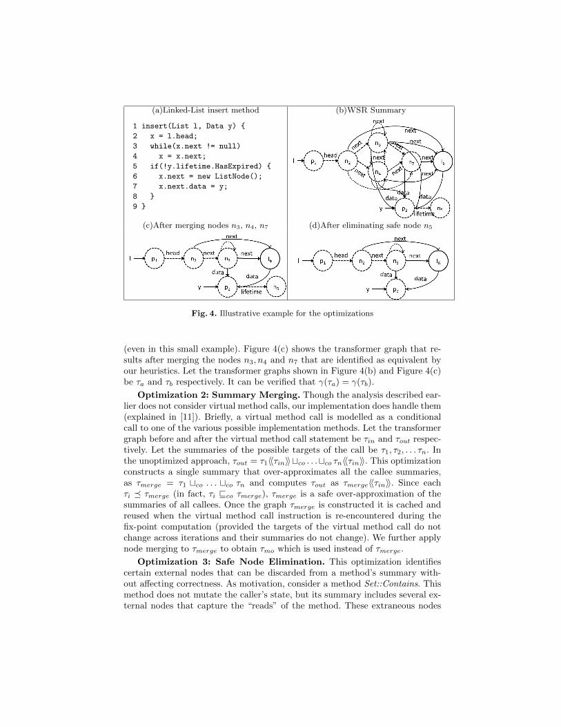
(a)Linked-List insert method (b)WSR Summary

1 insert(List l, Data y) {

2 x = l.head;

3 while(x.next != null)

4 x = x.next;

5 if(!y.lifetime.HasExpired) {

6 x.next = new ListNode();

7 x.next.data = y;

8 }

9 }

(c)After merging nodes n3, n4, n7 (d)After eliminating safe node n5

Fig. 4. Illustrative example for the optimizations

(even in this small example). Figure 4(c) shows the transformer graph that re-sults after merging the nodes n3, n4 and n7 that are identified as equivalent byour heuristics. Let the transformer graphs shown in Figure 4(b) and Figure 4(c)be τa and τb respectively. It can be verified that γ(τa) = γ(τb).

Optimization 2: Summary Merging. Though the analysis described ear-lier does not consider virtual method calls, our implementation does handle them(explained in [11]). Briefly, a virtual method call is modelled as a conditionalcall to one of the various possible implementation methods. Let the transformergraph before and after the virtual method call statement be τin and τout respec-tively. Let the summaries of the possible targets of the call be τ1, τ2, . . . τn. Inthe unoptimized approach, τout = τ1〈〈τin〉〉tco . . .tco τn〈〈τin〉〉. This optimizationconstructs a single summary that over-approximates all the callee summaries,as τmerge = τ1 tco . . . tco τn and computes τout as τmerge〈〈τin〉〉. Since eachτi � τmerge (in fact, τi vco τmerge), τmerge is a safe over-approximation of thesummaries of all callees. Once the graph τmerge is constructed it is cached andreused when the virtual method call instruction is re-encountered during thefix-point computation (provided the targets of the virtual method call do notchange across iterations and their summaries do not change). We further applynode merging to τmerge to obtain τmo which is used instead of τmerge.

Optimization 3: Safe Node Elimination. This optimization identifiescertain external nodes that can be discarded from a method’s summary with-out affecting correctness. As motivation, consider a method Set::Contains. Thismethod does not mutate the caller’s state, but its summary includes several ex-ternal nodes that capture the “reads” of the method. These extraneous nodes

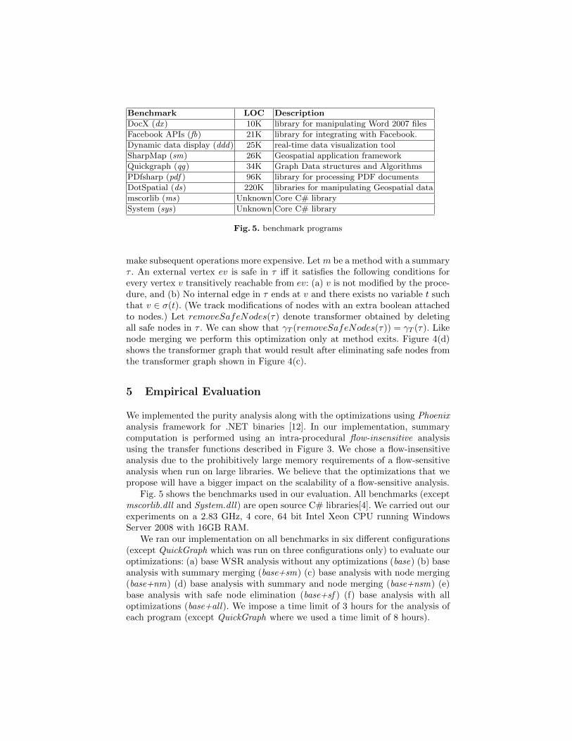
Benchmark LOC Description

DocX (dx ) 10K library for manipulating Word 2007 files

Facebook APIs (fb) 21K library for integrating with Facebook.

Dynamic data display (ddd) 25K real-time data visualization tool

SharpMap (sm) 26K Geospatial application framework

Quickgraph (qg) 34K Graph Data structures and Algorithms

PDfsharp (pdf ) 96K library for processing PDF documents

DotSpatial (ds) 220K libraries for manipulating Geospatial data

mscorlib (ms) Unknown Core C# library

System (sys) Unknown Core C# library

Fig. 5. benchmark programs

make subsequent operations more expensive. Let m be a method with a summaryτ . An external vertex ev is safe in τ iff it satisfies the following conditions forevery vertex v transitively reachable from ev: (a) v is not modified by the proce-dure, and (b) No internal edge in τ ends at v and there exists no variable t suchthat v ∈ σ(t). (We track modifications of nodes with an extra boolean attachedto nodes.) Let removeSafeNodes(τ) denote transformer obtained by deletingall safe nodes in τ . We can show that γT (removeSafeNodes(τ)) = γT (τ). Likenode merging we perform this optimization only at method exits. Figure 4(d)shows the transformer graph that would result after eliminating safe nodes fromthe transformer graph shown in Figure 4(c).

5 Empirical Evaluation

We implemented the purity analysis along with the optimizations using Phoenixanalysis framework for .NET binaries [12]. In our implementation, summarycomputation is performed using an intra-procedural flow-insensitive analysisusing the transfer functions described in Figure 3. We chose a flow-insensitiveanalysis due to the prohibitively large memory requirements of a flow-sensitiveanalysis when run on large libraries. We believe that the optimizations that wepropose will have a bigger impact on the scalability of a flow-sensitive analysis.

Fig. 5 shows the benchmarks used in our evaluation. All benchmarks (exceptmscorlib.dll and System.dll) are open source C# libraries[4]. We carried out ourexperiments on a 2.83 GHz, 4 core, 64 bit Intel Xeon CPU running WindowsServer 2008 with 16GB RAM.

We ran our implementation on all benchmarks in six different configurations(except QuickGraph which was run on three configurations only) to evaluate ouroptimizations: (a) base WSR analysis without any optimizations (base) (b) baseanalysis with summary merging (base+sm) (c) base analysis with node merging(base+nm) (d) base analysis with summary and node merging (base+nsm) (e)base analysis with safe node elimination (base+sf ) (f) base analysis with alloptimizations (base+all). We impose a time limit of 3 hours for the analysis ofeach program (except QuickGraph where we used a time limit of 8 hours).

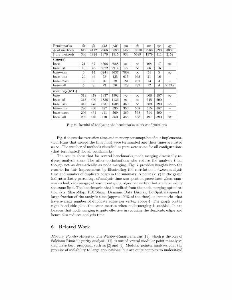
Benchmarks dx fb ddd pdf sm ds ms sys qg

# of methods 612 4112 2266 3883 1466 10810 2963 698 3380

Pure methods 340 1924 1370 1515 934 5699 1979 411 2152

time(s)

base 21 52 4696 5088 ∞ ∞ 108 17 ∞base+sf 19 46 3972 2914 ∞ ∞ 56 16 −base+sm 6 14 3244 4637 7009 ∞ 54 5 ∞base+nm 20 46 58 125 615 963 21 16 −base+nsm 5 9 26 79 181 251 13 4 −base+all 5 8 23 76 179 232 12 4 21718

memory(MB)

base 313 478 1937 1502 ∞ ∞ 608 387 ∞base+sf 313 460 1836 1136 ∞ ∞ 545 390 −base+sm 313 478 1937 1508 369 ∞ 589 390 ∞base+nm 296 460 427 535 356 568 515 387 −base+nsm 296 461 411 569 369 568 514 390 −base+all 296 446 410 550 356 568 497 390 703

Fig. 6. Results of analysing the benchmarks in six configurations

Fig. 6 shows the execution time and memory consumption of our implementa-tion. Runs that exceed the time limit were terminated and their times are listedas∞. The number of methods classified as pure were same for all configurations(that terminated) for all benchmarks.

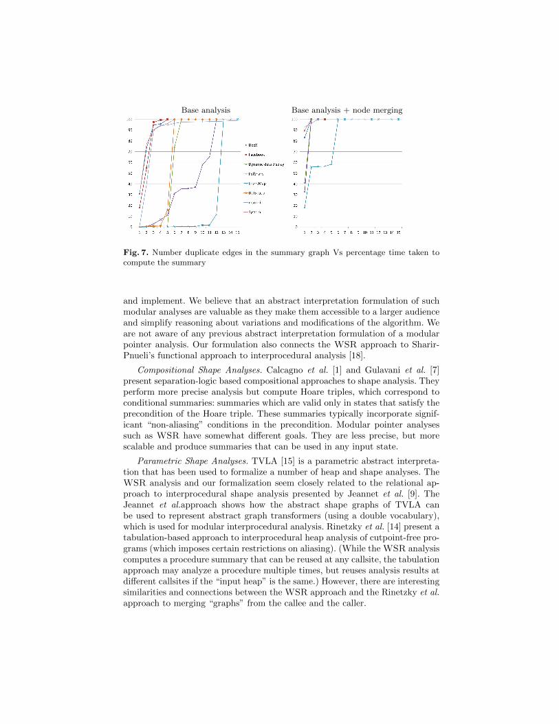
The results show that for several benchmarks, node merging drastically re-duces analysis time. The other optimizations also reduce the analysis time,though not as dramatically as node merging. Fig. 7 provides insights into thereasons for this improvement by illustrating the correlation between analysistime and number of duplicate edges in the summary. A point (x, y) in the graphindicates that y percentage of analysis time was spent on procedures whose sum-maries had, on average, at least x outgoing edges per vertex that are labelled bythe same field. The benchmarks that benefited from the node merging optimiza-tion (viz. SharpMap, PDFSharp, Dynamic Data Display, DotSpatial) spend alarge fraction of the analysis time (approx. 90% of the time) on summaries thathave average number of duplicate edges per vertex above 4. The graph on theright hand side plots the same metrics when node merging is enabled. It canbe seen that node merging is quite effective in reducing the duplicate edges andhence also reduces analysis time.

6 Related Work

Modular Pointer Analyses. The Whaley-Rinard analysis [19], which is the core ofSalcianu-Rinard’s purity analysis [17], is one of several modular pointer analysesthat have been proposed, such as [2] and [3]. Modular pointer analyses offer thepromise of scalability to large applications, but are quite complex to understand

Base analysis Base analysis + node merging

Fig. 7. Number duplicate edges in the summary graph Vs percentage time taken tocompute the summary

and implement. We believe that an abstract interpretation formulation of suchmodular analyses are valuable as they make them accessible to a larger audienceand simplify reasoning about variations and modifications of the algorithm. Weare not aware of any previous abstract interpretation formulation of a modularpointer analysis. Our formulation also connects the WSR approach to Sharir-Pnueli’s functional approach to interprocedural analysis [18].

Compositional Shape Analyses. Calcagno et al. [1] and Gulavani et al. [7]present separation-logic based compositional approaches to shape analysis. Theyperform more precise analysis but compute Hoare triples, which correspond toconditional summaries: summaries which are valid only in states that satisfy theprecondition of the Hoare triple. These summaries typically incorporate signif-icant “non-aliasing” conditions in the precondition. Modular pointer analysessuch as WSR have somewhat different goals. They are less precise, but morescalable and produce summaries that can be used in any input state.

Parametric Shape Analyses. TVLA [15] is a parametric abstract interpreta-tion that has been used to formalize a number of heap and shape analyses. TheWSR analysis and our formalization seem closely related to the relational ap-proach to interprocedural shape analysis presented by Jeannet et al. [9]. TheJeannet et al.approach shows how the abstract shape graphs of TVLA canbe used to represent abstract graph transformers (using a double vocabulary),which is used for modular interprocedural analysis. Rinetzky et al. [14] present atabulation-based approach to interprocedural heap analysis of cutpoint-free pro-grams (which imposes certain restrictions on aliasing). (While the WSR analysiscomputes a procedure summary that can be reused at any callsite, the tabulationapproach may analyze a procedure multiple times, but reuses analysis results atdifferent callsites if the “input heap” is the same.) However, there are interestingsimilarities and connections between the WSR approach and the Rinetzky et al.approach to merging “graphs” from the callee and the caller.

Modularity In Interprocedural Analysis. While the WSR analysis is modularin the absence of recursion, recursive procedures must be analyzed together. Ourexperience has shown that large strongly connected components of proceduresin the call-graph can be a bottleneck in analyzing large libraries. An interestingdirection for future work is to explore techniques that can be used to achievemodularity even in the presence of recursion, e.g., see [6].

References

1. Calcagno, C., Distefano, D., O’Hearn, P.W., Yang, H.: Compositional shape anal-ysis by means of bi-abduction. In: POPL. pp. 289–300 (2009)

2. Chatterjee, R., Ryder, B.G., Landi, W.A.: Relevant context inference. In: POPL.pp. 133–146 (1999)

3. Cheng, B.C., Hwu, W.M.W.: Modular interprocedural pointer analysis using accesspaths: design, implementation, and evaluation. In: PLDI. pp. 57–69 (2000)

4. Codeplex. http://www.codeplex.com (March 2011)5. Cousot, P., Cousot, R.: Abstract interpretation frameworks. J. Log. Comput. 2(4),

511–547 (1992)6. Cousot, P., Cousot, R.: Modular static program analysis. In: CC. pp. 159–178

(2002)7. Gulavani, B.S., Chakraborty, S., Ramalingam, G., Nori, A.V.: Bottom-up shape

analysis. In: SAS. pp. 188–204 (2009)8. Gulavani, B.S., Henzinger, T.A., Kannan, Y., Nori, A.V., Rajamani, S.K.: SYN-

ERGY: a new algorithm for property checking. In: FSE. pp. 117–127 (2006)9. Jeannet, B., Loginov, A., Reps, T., Sagiv, M.: A relational approach to interpro-

cedural shape analysis. ACM Trans. Program. Lang. Syst. 32, 5:1–5:52 (February2010), http://doi.acm.org/10.1145/1667048.1667050

10. Knoop, J., Steffen, B.: The interprocedural coincidence theorem. In: CC. pp. 125–140 (1992)

11. Madhavan, R., Ramalingam, G., Vaswani, K.: Purity analysis: An abstract inter-pretation formulation, (Forthcoming) Tech. rep., Microsoft Research, India.

12. Phoenix. https://connect.microsoft.com/Phoenix (March 2011)13. Prabhu, P., Ramalingam, G., Vaswani, K.: Safe programmable speculative paral-

lelism. In: PLDI. pp. 50–61 (2010)14. Rinetzky, N., Sagiv, M., Yahav, E.: Interprocedural shape analysis for cutpoint-free

programs. In: SAS. pp. 284–302 (2005)15. Sagiv, S., Reps, T.W., Wilhelm, R.: Parametric shape analysis via 3-valued logic.

In: POPL. pp. 105–118 (1999)16. Salcianu, A.D.: Pointer Analysis and its Applications for Java Programs. Master’s

thesis, Massachusetts institute of technology (2001)17. Salcianu, A.D., Rinard, M.C.: Purity and side effect analysis for java programs. In:

In VMCAI. Springer-Verlag (2005)18. Sharir, M., Pnueli, A.: Two approaches to interprocedural data flow analysis. In:

Program Flow Analysis: Theory and Applications. pp. 189–234 (1981)19. Whaley, J., Rinard, M.C.: Compositional pointer and escape analysis for java pro-

grams. In: OOPSLA. pp. 187–206 (1999)