python programming for data processing and climate...
TRANSCRIPT
Python Programmingfor
Data Processing and Climate Analysis
Jules Kouatchou and Hamid [email protected] and [email protected]
Goddard Space Flight CenterSoftware System Support Office
Code 610.3
April 8, 2013
Background Information
Training Objectives
We want to introduce:
Basic concepts of Python programming
Array manipulations
Handling of files
2D visualization
EOFs
J. Kouatchou and H. Oloso (SSSO) EOFs with Python April 8, 2013 2 / 33
Background Information
Special Topics
Based on the feedback we have received so far, we plan to have a hand-onpresentation on the following topic(s):
F2Py:
Python interface to Fortran
Date: April 29, 2013 at 1:30pm
iPython Notebook:
A web-based interactive computational environment
Tentative Date: TBD
J. Kouatchou and H. Oloso (SSSO) EOFs with Python April 8, 2013 3 / 33
Background Information
Obtaining the Material
Slides for this session of the training are available from:
https://modelingguru.nasa.gov/docs/DOC-2322
You can obtain materials presented here on discover at
/discover/nobackup/jkouatch/pythonTrainingGSFC.tar.gz
After you untar the above file, you will obtain the directorypythonTrainingGSFC/ that contains:
Examples/
Slides/
J. Kouatchou and H. Oloso (SSSO) EOFs with Python April 8, 2013 4 / 33

Background Information
Settings on discover
To use the Python distribution:
module load other/comp/gcc-4.5-sp1
module load lib/mkl-10.1.2.024
module load other/SIVO-PyD/spd_1.9.0_gcc-4.5-sp1
To use uvcdat:
module load other/uvcdat-1.2-gcc-4.7.1
J. Kouatchou and H. Oloso (SSSO) EOFs with Python April 8, 2013 5 / 33
Background Information
What Will be Covered Today
1 Basic Introduction to EOF
2 Data Source & EOFs with NCL
3 Two Approaches for Doing EOFs
CDATNumpy
J. Kouatchou and H. Oloso (SSSO) EOFs with Python April 8, 2013 6 / 33

Basic Concepts
Useful Links on EOFs
EOF Analysis by Cygnus Research International,http://www.cygres.com/OcnPageE/Glosry/OcnEof1E.html
Time Series Tutorial Notes by Jin-Yi Yu, http://www.ess.uci.edu/~yu/class/ess210b/lecture.5.EOF.all.pdf
J. Kouatchou and H. Oloso (SSSO) EOFs with Python April 8, 2013 7 / 33
Basic Concepts
What is EOFs Analysis?
Empirical Orthogonal Function (EOF) analysis attempts to find arelatively small number of independent variables (predictors; factors)which convey as much of the original information as possible withoutredundancy.
EOF analysis can be used to explore the structure of the variabilitywithin a data set in a objective way, and to analyze relationshipswithin a set of variables.
EOF analysis is also called principal component analysis or factoranalysis.
J. Kouatchou and H. Oloso (SSSO) EOFs with Python April 8, 2013 8 / 33

Basic Concepts
What Does EFO Analysis Do?
Uses a set of orthogonal functions (EOFs) to represent a time series in thefollowing way
Z (x , y , t) =N∑
k=1
Pk(t) × Ek(x , y)
Z (x , y , t) is the original time series as a function of time (t) andspace (x , y).
Ek(x , y) show the the spatial structures (x , y) of the major factorsthat can account for the temporal variations of Z .
Pk(t) is the principal component that tells you how the amplitude ofeach EOF varies with time.
J. Kouatchou and H. Oloso (SSSO) EOFs with Python April 8, 2013 9 / 33

Basic Concepts
What Does EOF Analysis Provides?
1 A set of EOF loading patterns (eigenvectors)
2 A set of corresponding amplitudes (temporal scores)
3 A set of corresponding variances accounted for (eigenvalues)
J. Kouatchou and H. Oloso (SSSO) EOFs with Python April 8, 2013 10 / 33

Source of Data
Data
We use Sea Level Pressure from NCEP/NCAR Reanalysis 1
Monthly means from 1948 to present
2.5 × 2.5 grid resolution
Global data
J. Kouatchou and H. Oloso (SSSO) EOFs with Python April 8, 2013 11 / 33

Source of Data
Verification
We can use NCAR Command Language (NCL) to perform EOFcalcilations.
Show good demonstration of typical steps (data sub-setting, seasonaltime averaging, plotting of EOFs, etc)
For plots: http://www.ncl.ucar.edu/Applications/eof.shtml
For source code:http://www.ncl.ucar.edu/Applications/Scripts/eof_1.ncl
J. Kouatchou and H. Oloso (SSSO) EOFs with Python April 8, 2013 12 / 33

Source of Data
NCL: Seasonal SLP Plot
J. Kouatchou and H. Oloso (SSSO) EOFs with Python April 8, 2013 13 / 33
Approaches for Doing EOFs
What is eof2?
Python package for performing EOF analysis on spatial-temporal datasets
Suitable for large data sets
Transparent handling of missing values
Work both within a CDAT environment or as a stand-alone package
Provides two interfaces (supporting the same sets of operations) forEOF analysis:
1 Numpy arrays2 cdms2 variables (which preserves metadata)
For more information: http://ajdawson.github.com/eof2/
J. Kouatchou and H. Oloso (SSSO) EOFs with Python April 8, 2013 14 / 33
Approaches for Doing EOFs
eof2 Solver
Uses SVD
Expects as input a spatial-temporal field represented a an array(Numpy array or cdms2 variable) of two or more dimensions.
Internally, any missing values in the array are identified and removed.
The EOF solution is computed when an instance of eof2.Eof (forcdms2) or eof2.EofSolver (for Numpy) is initialized.
J. Kouatchou and H. Oloso (SSSO) EOFs with Python April 8, 2013 15 / 33

Approaches for Doing EOFs
Main eof2 Functions
Here are some functions associated with the solver:
eofs: Array with the ordered EOFs along
the first dimension
eofsAsCorrelation: EOFs scaled as the correlation of
the PCs with the original field.
eofsAsCovariance: EOFs scaled as the covariance of
the PCs with the original field.
eigenvalues: Eigenvalues (decreasing variances)
associated with each EOF
pcs: Principal component time series (PCs).
Array where the columns are the ordered PCs.
J. Kouatchou and H. Oloso (SSSO) EOFs with Python April 8, 2013 16 / 33

Approaches for Doing EOFs
How to Use eof2?
1 from eof2 import Eof
2 #from eof2 import EofSolver
3 ...
4 # Initialize and Eof object.
5 # Square -root of cosine of latitude weights are used.
6 solver = Eof(myData , weights=’coslat ’)
7
8 #coslat = np.cos (np. deg2rad ( lats ))
9 #wgts = np. sqrt ( coslat )[... , np. newaxis ]
10 #solver = EofSolver (myData , weights = wgts )
11
12 # Retrieve the first two EOFs.
13 eofs = solver.eofs(neofs =2)
14
15 # Retrieve the eigenvalues
16 eigenVals = solver.eigenvalues ()
J. Kouatchou and H. Oloso (SSSO) EOFs with Python April 8, 2013 17 / 33
Approaches for Doing EOFs CDAT
What is CDAT?
CDAT: Climate Data Analysis Tools
Software ”glued” under the Python framework
CDAT packages use:
cdms2 - Climate Data Management System (file I/O, variables, types,metadata, grids)cdutil - Climate Data Specific Utilities (spatial and temporal averages,custom seasons, climatologies)vcs - Visualization and Control System (manages graphical window:picture template, graphical methods, data)
J. Kouatchou and H. Oloso (SSSO) EOFs with Python April 8, 2013 18 / 33

Approaches for Doing EOFs CDAT
CDAT: Reading Data and Calculations
1 f = cdms2.open(’slp.mon.mean. n c )
2 slp = f(’slp’, time=(’1979’,’2003’), \
3 latitude =(85,20) , longitude =( -70 ,40))
4 f.close ()
5
6 # Put time point at the beginning instead of middle of month
7 cdutil.setTimeBoundsMonthly(slp)
8
9 # Extract Dec -Jan -Feb seasons
10 djfslp = cdutil.DJF(slp)
11
12 coslat = np.cos(np.deg2rad(slp.getLatitude ()[:]))
13 wgts = np.sqrt(coslat )[..., np.newaxis]
14
15 slpsolver = Eof(djfslp , weights=wgts)
16 eofs = slpsolver.eofs(neofs =3)
17 eigenvalueVec = slpsolver.eigenvalues ()J. Kouatchou and H. Oloso (SSSO) EOFs with Python April 8, 2013 19 / 33

Approaches for Doing EOFs CDAT
CDAT: Looking at the Results
1 print eigenvalueVec ()
2 print 100* eigenvalueVec ()[0:3]/ fsum(eigenvalueVec ())
3
4 # Initialise a VCS canvas for plotting
5 p = vcs.init()
6
7 t=p.createtemplate(’new’)
8 t.scale (0.5)
9
10 # Plot the first EOF
11 p.plot(eofs[0],’default ’,’isofill ’)
J. Kouatchou and H. Oloso (SSSO) EOFs with Python April 8, 2013 20 / 33

Approaches for Doing EOFs CDAT
CDAT: Seasonal SLP Plot
J. Kouatchou and H. Oloso (SSSO) EOFs with Python April 8, 2013 21 / 33
Approaches for Doing EOFs Numpy and eof2
How Do We Do EOF?
We use:
netCDF4: to read the dataset
Numpy: to manipulate arrays
eof2: for EOF calculations
Matplotlib/Basemap: for plotting
J. Kouatchou and H. Oloso (SSSO) EOFs with Python April 8, 2013 22 / 33
Approaches for Doing EOFs Numpy and eof2
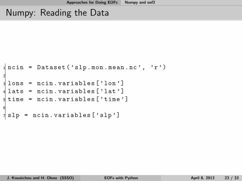
Numpy: Reading the Data
1 ncin = Dataset(’slp.mon.mean.nc’, ’r’)
2
3 lons = ncin.variables[’lon’]
4 lats = ncin.variables[’lat’]
5 time = ncin.variables[’time’]
6
7 slp = ncin.variables[’slp’]
J. Kouatchou and H. Oloso (SSSO) EOFs with Python April 8, 2013 23 / 33
Approaches for Doing EOFs Numpy and eof2
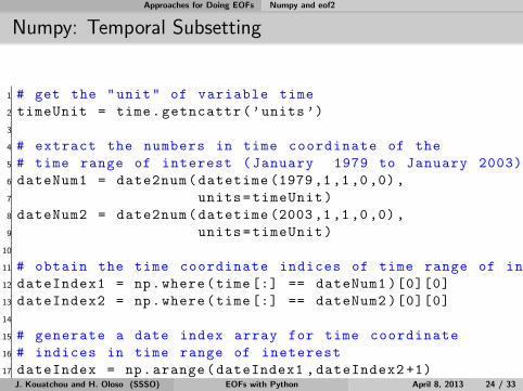
Numpy: Temporal Subsetting
1 # get the "unit" of variable time
2 timeUnit = time.getncattr(’units ’)
3
4 # extract the numbers in time coordinate of the
5 # time range of interest (January 1979 to January 2003)
6 dateNum1 = date2num(datetime (1979,1,1,0,0),
7 units=timeUnit)
8 dateNum2 = date2num(datetime (2003,1,1,0,0),
9 units=timeUnit)
10
11 # obtain the time coordinate indices of time range of interest
12 dateIndex1 = np.where(time [:] == dateNum1 )[0][0]
13 dateIndex2 = np.where(time [:] == dateNum2 )[0][0]
14
15 # generate a date index array for time coordinate
16 # indices in time range of ineterest
17 dateIndex = np.arange(dateIndex1 ,dateIndex2 +1)J. Kouatchou and H. Oloso (SSSO) EOFs with Python April 8, 2013 24 / 33

Approaches for Doing EOFs Numpy and eof2
Numpy: Spatial Subsetting
1 # Realign SLP so that longitude goes from -180 to 180
2 slpShift = np.zeros ((slp.shape [0],slp.shape [1],
3 slp.shape [2]), dtype=np.float32)
4 for i in range(slp.shape [0]):
5 slpShift[i,:,:], lonShift =
6 shiftgrid (180. ,slp[i,:,:],lon[:],start=False)
7
8 # Subsetting and Resersing latitudes
9 latIndex = np. nonzero (( lat [:: -1]>= 25 ) & \
10 (lat [:: -1]<= 80 ))[0]
11 # Subsetting longitudes
12 lonIndex = np. nonzero (( lonShift >= -70 ) & \
13 (lonShift <=40 ))[0]
14
15 # extract the desired data subset for analysis
16 slpSubset=slpShift [:,::-1,:][ dateIndex [0]: dateIndex [-1]+1,
17 latIndex [0]: latIndex [-1]+1, lonIndex]J. Kouatchou and H. Oloso (SSSO) EOFs with Python April 8, 2013 25 / 33

Approaches for Doing EOFs Numpy and eof2
Numpy: Seasonal Climatology
1 # Compute Dec -Jan -Feb seasonal climatology
2 slpDJF = np.zeros ((25, latIndex.shape[0],
3 lonIndex.shape [0]), dtype=np.float32)
4 slpDJF [0,:,:] = (slpSubset [0 ,: ,:]*31.+
5 slpSubset [1 ,: ,:]*28.)/(31.+28.) # first season
6 for i in range (1 ,24):
7 if np.mod(i,4) == 1: # leap year
8 slpDJF[i,:,:] = (( slpSubset [12.*i-1.,:,:] + \
9 slpSubset [12.*i,: ,:])*31. + \
10 slpSubset [12.*i+1. ,: ,:]*29.) / (31.+31.+29.)
11 else: # non leap year
12 slpDJF[i,:,:] = (( slpSubset [12.*i-1.,:,:] +
13 slpSubset [12.*i ,: ,:])*31. +
14 slpSubset [12.*i+1. ,: ,:]*28.) / (31.+31.+28.)
15
16 slpDJF [24,:,:] = (slpSubset [-2,:,:]+
17 slpSubset [ -1 ,: ,:])*31./62.J. Kouatchou and H. Oloso (SSSO) EOFs with Python April 8, 2013 26 / 33

Approaches for Doing EOFs Numpy and eof2
Numpy: EOF Solver
1 #----------------------------------------------
2 # Create an EOF solver to do the EOF analysis.
3 # Square -root of cosine of latitude weights are
4 # applied before the computation of EOFs.
5 #----------------------------------------------
6 coslat = np.cos(np.deg2rad(lat [:: -1][ latIndex ]))
7 wgts = np.sqrt(coslat )[..., np.newaxis]
8 solver = EofSolver(slpDJF , weights=wgts)
9
10 # extract eignevalues
11 eigenValues = solver.eigenvalues ()
12
13 # compute % contribution of each EOF
14 percentContrib = eigenValues *100./ np.sum(eigenValues)
15
16 # compute the first three leading EOFs (EOFs 0, 1 and 2)
17 eofs = solver.eofs(neofs =3)J. Kouatchou and H. Oloso (SSSO) EOFs with Python April 8, 2013 27 / 33
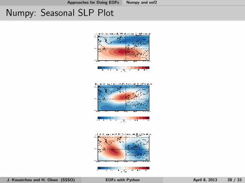
Approaches for Doing EOFs Numpy and eof2
Numpy: Seasonal SLP Plot
J. Kouatchou and H. Oloso (SSSO) EOFs with Python April 8, 2013 28 / 33

Approaches for Doing EOFs Numpy and eof2
Numpy: Reading the Data Global Data
1 ncin = Dataset(’slp.mon.mean.nc’, ’r’)
2
3 lons = ncin.variables[’lon’][:]
4 lats = ncin.variables[’lat’][:]
5 time = ncin.variables[’time’][:]
6
7 slp = ncin.variables[’slp’][:]
8
9 ncin.close()
J. Kouatchou and H. Oloso (SSSO) EOFs with Python April 8, 2013 29 / 33

Approaches for Doing EOFs Numpy and eof2
Numpy: EOF Solver
1 #----------------------------------------------
2 # Create an EOF solver to do the EOF analysis.
3 # Square -root of cosine of latitude weights are
4 # applied before the computation of EOFs.
5 #----------------------------------------------
6 coslat = np.cos(np.deg2rad(lats))
7 wgts = np.sqrt(coslat )[..., np.newaxis]
8 solver = EofSolver(slp , weights=wgts)
9
10 #---------------------------------------------------
11 # Retrieve the leading EOF , expressed as the
12 # correlation between the leading PC time series and
13 # the input SLP at each grid point , and the leading
14 # PC time series itself.
15 #---------------------------------------------------
16 eof1 = solver.eofsAsCorrelation(neofs =1)
17 pc1 = solver.pcs(npcs=1, pcscaling =1)J. Kouatchou and H. Oloso (SSSO) EOFs with Python April 8, 2013 30 / 33

Approaches for Doing EOFs Numpy and eof2
Numpy: SLP EOF1 Expressed as Correlation
J. Kouatchou and H. Oloso (SSSO) EOFs with Python April 8, 2013 31 / 33

Approaches for Doing EOFs Numpy and eof2
Numpy: SLP PC1 Time Series
J. Kouatchou and H. Oloso (SSSO) EOFs with Python April 8, 2013 32 / 33

Approaches for Doing EOFs Numpy and eof2
References I
Johnny Wei-Bing Lin, A Hands-On Introduction to Using Python inthe Atmospheric and Oceanic Sciences,http://www.johnny-lin.com/pyintro, 2012.
Hans Petter Langtangen, A Primer on Scientific Programming withPython, Springer, 2009.
Drew McCormack, Scientific Scripting with Python, 2009.
Sandro Tosi, Matplotlib for Python Developers, 2009.
A. Hannachi, I. T. Jolliffe and D. B. Stephenson, Empirical orthogonalfunctions and related techniques in atmospheric science: A review, Int.J. Climatol. 27: 1119–1152 (2007).
J. Kouatchou and H. Oloso (SSSO) EOFs with Python April 8, 2013 33 / 33