qcd at the lhchacol13.physik.uni-freiburg.de/graduiertenkolleg/klausurtagungen/... · ( higher...
TRANSCRIPT

Lectures onLectures on
QCD at the LHC
James StirlingCambridge UniversityCambridge University
Gutach Bleibach 25 November 2010Gutach Bleibach, 25 November 2010
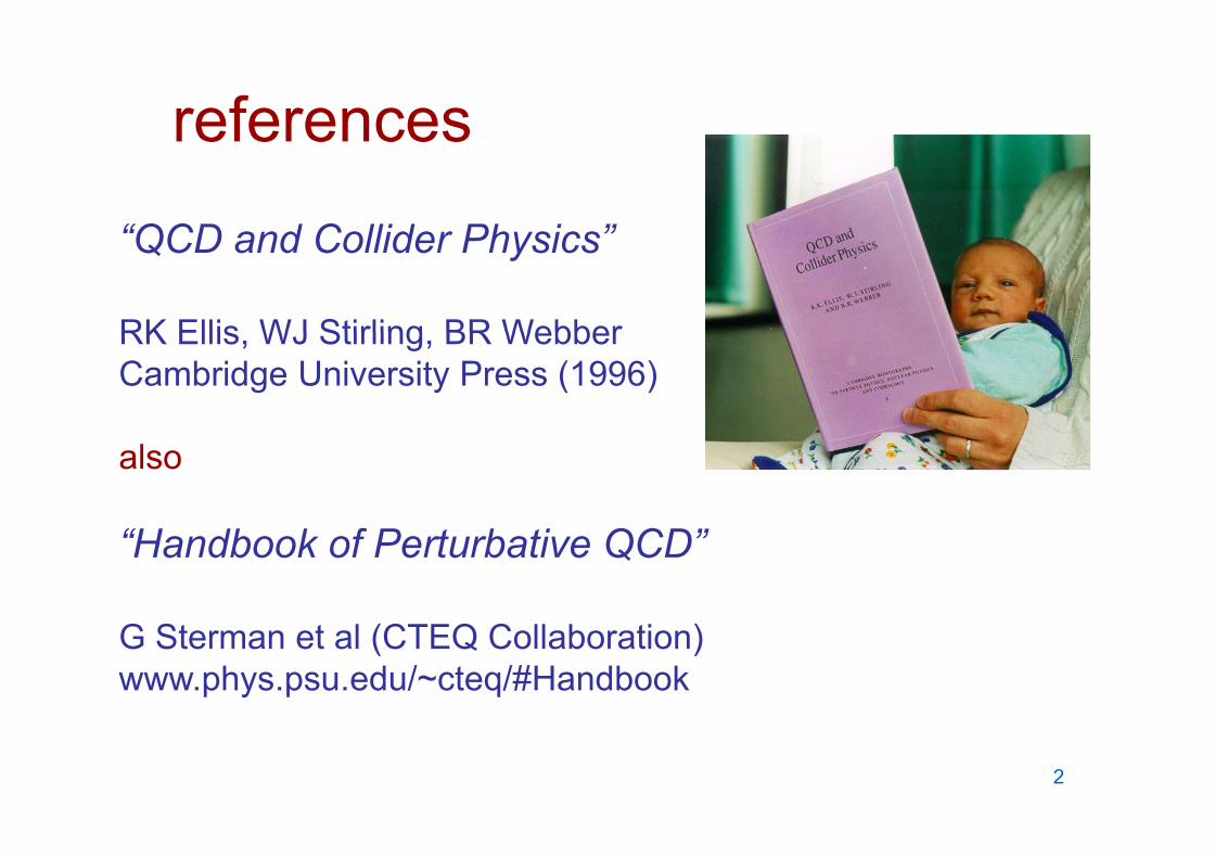
referencesreferences
“QCD and Collider Physics”QCD and Collider Physics
RK Ellis WJ Stirling BR WebberRK Ellis, WJ Stirling, BR WebberCambridge University Press (1996)
also
“Handbook of Perturbative QCD”
G S (C Q C )G Sterman et al (CTEQ Collaboration)www.phys.psu.edu/~cteq/#Handbook
2

… and
“Hard Interactions ofHard Interactions of Quarks and Gluons: a Primer for LHC Physics ”Primer for LHC Physics
JM Campbell JW Huston WJJM Campbell, JW Huston, WJ Stirling (CSH)
arxiv.org/abs/hep-ph/0611148
Rep Prog Phys 70 89 (2007)Rep. Prog. Phys. 70, 89 (2007)
3

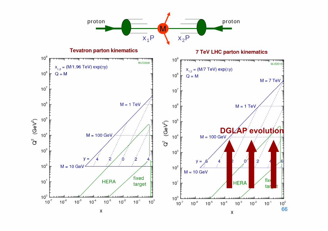
past, present and future proton/antiproton colliderscolliders…
Tevatron (1987→)Fermilab
proton-antiproton collisionsS = 1.8, 1.96 TeV,
tc b W,Z H, SUSY,...?
SppS (1981 → 1990)CERNproton-antiproton
-1970 1980 1990 2000 20202010
LHC (2009 → )CERNproton-proton and
p pcollisionsS = 540, 630 GeV
p pheavy ion collisionsS = 7 – 14 TeV
4
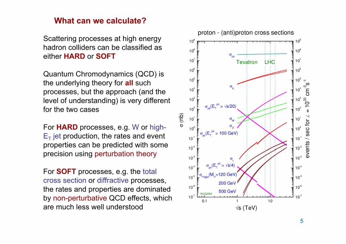
Scattering processes at high energy
What can we calculate?
Scattering processes at high energy hadron colliders can be classified as either HARD or SOFT
Quantum Chromodynamics (QCD) is the underlying theory for all such processes, but the approach (and the p , pp (level of understanding) is very different for the two cases
For HARD processes, e.g. W or high-ET jet production, the rates and event properties can be predicted with some precision using perturbation theory
For SOFT processes, e.g. the total ffcross section or diffractive processes,
the rates and properties are dominated by non-perturbative QCD effects, which
h l ll d t dare much less well understood
5

Outline• Basics I: introduction to QCD
– Motivation, Lagrangian, Feynman rules– the running coupling S : theory and measurement
l t t f th QCD t b ti i– general structure of the QCD perturbation series
• Basics II: partons– basic parton model ideas for DIS– scaling violation & DGLAP– parton distribution functions– hard scattering & basic kinematics– the Drell-Yan process in the parton model– factorisation– parton luminosity functions
• Application to the LHC– leading-order calculations– beyond leading order: higher-order perturbative QCD corrections– benchmark cross sections– beyond perturbation theory
• Sudakov logs and resummation• parton showering models (basic concepts only!)• the role of non-perturbative contributions: intrinsic kT
6

1introduction to QCDintroduction to QCD
• Motivation, Lagrangian, Feynman rules
• the running coupling S : theory and measurementS
• general structure of the QCD perturbation series
7
Quantum ChromodynamicsQuantum Chromodynamics- a Yang-Mills gauge theory with SU(3) symmetry
Rationale – evidence that quarks come in 3 colours
• ++ = (uuu) requires additional (≥3) internal degrees of freedom to satisfy Fermi-Dirac statisticsy
• cross sections and decay rates, e.g. (e+e- hadrons) y g ( )Nc and (0) Nc
2 , imply Nc = 3.0 ± ...
Th t k i t i l t d iThus, put quarks in triplets, iq = (q,q,q), and require
invariance under local SU(3) transformations
8
QCD LagrangianQCD Lagrangian
where • i th QCD li t t• gs is the QCD coupling constant• fabc are the structure constants of SU(3): [Ta,Tb] = i fabc Tc
(a b c = 1 8)(a,b,c = 1,…8)• A
a are the 8 gluon fields • Tij
a are 8 ‘colour matrices’, i.e. generators of the SU(3)Tij are 8 colour matrices , i.e. generators of the SU(3) transformation acting on the fundamental (triplet) representation: Gell-Mann 33
matrices, see ESW9
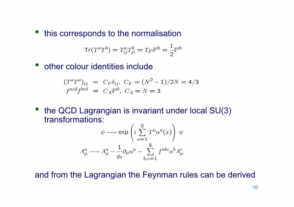
• this corresponds to the normalisation• this corresponds to the normalisation
• other colour identities include
• the QCD Lagrangian is invariant under local SU(3) transformations:
and from the Lagrangian the Feynman rules can be derivedand from the Lagrangian the Feynman rules can be derived10

Feynman Rules for QCD
(covariant gauge)
11

• Note: gauge fixing – to quantise the theory and reduce the number of degrees of freedom of the gauge fields,the number of degrees of freedom of the gauge fields, need to introduce a gauge fixing term:
• these are covariant gauges, and additional ghost fieldsare req iredare required….
a
cp
b
k
cb
or
• these are non-covariant (“axial”) gauges… no ghosts ( ) g g grequired!
12
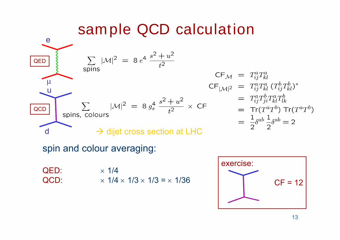
sample QCD calculatione
QED
e
u
QCD
u
spin and colour averaging:
d dijet cross section at LHC
spin and colour averaging:
QED: 1/4exercise:
QCD: 1/4 1/3 1/3 = 1/36 CF = 12
13

renormalised coupling constants• when we renormalise the coupling constant in a QFT, we introduce a
renormalisation scale,
+ + + ….+ + + ….=
• … and because there are additional diagrams (interactions) in QCD, the b,c,… coefficients in QCD and QED will be different
bare coupling u/v cut-off for divergent loop integrals
, ,
• how does g() depend on ?
14

the QCD running coupling
• and by explicit calculation gand by explicit calculation QCD
QED
• formally
the function
• in principle, can solve the differential equation in terms of g(0), to be determined from experiment
15

• explicit leading order solutiong
QCD
QED
g
• QED
• QCD
from experiment
or (historically)
16

Asymptotic Freedom
“What this year's Laureates discovered was something that, at first sight seemed completelfirst sight, seemed completely contradictory. The interpretation of their mathematical result was that the closer the quarks are to each othercloser the quarks are to each other, the weaker is the 'colour charge'. When the quarks are really close to each other the force is so weak thateach other, the force is so weak that they behave almost as free particles. This phenomenon is called ‘asymptotic freedom’. The converseasymptotic freedom . The converse is true when the quarks move apart: the force becomes stronger when the distance increases.”
αS(r)
171/r

beyond leading order• many QCD cross sections are nowadays measured to high accuracy thereforemany QCD cross sections are nowadays measured to high accuracy, therefore
need to take into account higher order (HO) corrections, e.g. 1 + c S , including in the definition ofS
• recall
thi t ti l ti ld h d fi d th lithis represents a particular convention; we could have defined another coupling, g’ , by say replacing 2 or by using the ggg vertex:
• in general, the coupling constants in 2 different schemes will be related by:
18

minimal subtraction renormalisation schemes• instead of regularising integrals like ∫d4k/k4 with a u/v cut-off M, reduce the
number of dimensions to N < 4; introduce ε = 2 – N/2
ith l M di th l d b 1/ lwith log M divergences then replaced by 1/ε poles
• MS prescription: when calculating a divergent scattering amplitude b d l di d bt t ff th 1/ l d l b thbeyond leading order, subtract off the 1/ε poles and replace g0 by the renormalised coupling g()
• b t ti th t th l l i th bi ti• but notice that the poles always appear in the combination
• … so instead subtract off this combination; this is the modified minimal subtraction (MS) scheme, widely used in practical pQCD calculations
19

QCD coupling beyond leading order
• the LO NLO solution is
• so for LO/NLO/NNLO pQCD phenomenology we need to pQ p gyinclude 0, 1, 2 in the definition of S
• see e g ESW for treatment of non-zero quark masses etcsee e.g. ESW for treatment of non zero quark masses etc20

techniques for S measurements
gluon
heavyquark hadrons
jets
lepton quark
g
+e+e-
theoretical issues:
DIS
theoretical issues:• HO pQCD corrections ( scale dependence)• Q-2n power corrections DIS • Q 2n power corrections ( higher twist, hadronisation)
21
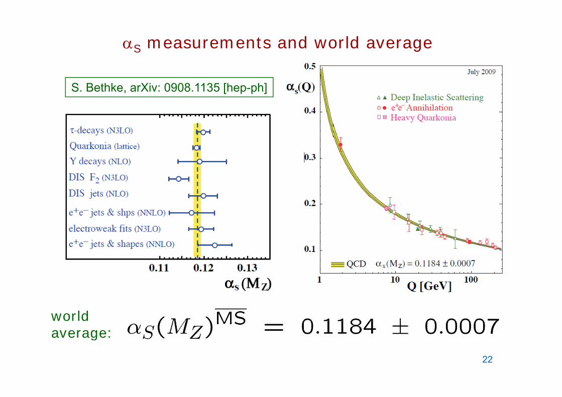
S measurements and world average
S. Bethke, arXiv: 0908.1135 [hep-ph]
worldaverage:average:
22

note the “shrinking error” effectnote the shrinking error effect…
• from the basic (LO) definitionfrom the basic (LO) definition
• therefore a precise measurement of the couplingtherefore a precise measurement of the coupling at a small scale Q can given improved precision on the fundamental parameter S(MZ
2)• however, the small-scale determination may be
more “contaminated” by power corrections or other non perturbative effectsother non-perturbative effects
23

general structure of a QCD perturbation series
• choose a renormalisation scheme (e.g. MSbar)• calculate cross section to some order (e g NLO)calculate cross section to some order (e.g. NLO)
physical process dependent coefficients renormalisation
• note d/d=0 “to all orders” but in practice
p yvariable(s)
p pdepending on P scale
note d/d 0 to all orders , but in practiced(N+n)/d= O((N+n)S
N+n+1)
• can try to help convergence by using a “physical scale choice”, ~ P , e.g. = MZ or = ET
jet at LHC
• what if there is a wide range of P’s in the process, e.g. W + n jets? 24

the higher the order in perturbation theory, the weaker the scale dependence …weaker the scale dependence …
Anastasiou, Dixon,Anastasiou, Dixon, Melnikov, Petriello, 2004
• l l i ti t i t h• only scale variation uncertainty shown• central values calculated for a fixed set pdfs with a fixed value of S(MZ
2)25

Basics of QCD - SummaryBasics of QCD Summary
1
αS(μ) non-perturbativegluon
gS Taij
gluon
gS fabc
perturbativequark quark2/4
gluongluon
• renormalisation of the coupling
0μ (GeV)
S = gS2/4
• colour matrix algebra
26

2partonspartons
• basic parton model ideas for DIS
• scaling violation & DGLAP
• parton distribution functions
27

but protons are not fundamental –h t h h th llid ?what happens when they collide?
?
Most of the time – nothing of much interest, the protons break up and the final state consists of many low energy particles (pions, kaons, photons, neutrons, ….)
But, occasionally, a parton (quark or gluon) from each proton can undergo a ‘hard scattering’
28

hard scattering in hadron-hadron collisions
higher-order pQCD corrections; i di ti j t
paccompanying radiation, jets
parton distribution X = W, Z, top, jets,d st but ofunctions
, , p, j ,SUSY, H, …
underlying eventp
for inclusive production, the basic calculational framework is provided by the QCD FACTORISATION THEOREM:
29

deep inelastic scattering
electron• variables
2 2q
p
Q2 = –q2
x = Q2 /2p·q (Bjorken x)pX proton
x Q /2p q (Bjorken x)
( y = Q2 /x s )
• resolution • inelasticity
QQh GeVm102 16 222
2
pX MMQQx
at HERA, Q2 < 105 GeV2
> 10-18 m = r /1000 0 < x 1
> 10 18 m = rp/100030

structure functions• in general, we can write y2,2(1-y)g
Q-4
F1, F2
where the Fi(x,Q2) are calledstructure functions SLAC, ~1970
• experimentally, 2 2 1.0
1.2
Q2 (GeV2) 1.5
SLAC, 1970
for Q2 > 1 GeV2
– Fi(x,Q2) Fi(x) 0.6
0.8
1.0 3.0 5.0 8.0 11.0 8.75 24.5230(x
,Q2 )
“scaling”– F2(x) 2 x F1(x) 0.2
0.4
230 80 800 8000
F 2
0.0 0.1 0.2 0.3 0.4 0.5 0.6 0.7 0.80.0
Bjorken 1968 31

toy model• suppose that the electron scatters off a pointlike,
~massless, spin ½ particle a of charge ea moving collinear with the parent proton with four-momentum p =pwith the parent proton with four momentum pa
p
• calculate the scattering cross section ea ea
k k’
pq
k k
• Exercise: show that if a has spin zero then F = 0• Exercise: show that if a has spin-zero, then F1 = 032
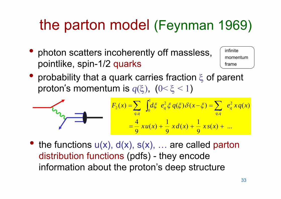
the parton model (Feynman 1969)
• photon scatters incoherently off massless
p ( y )
infinitephoton scatters incoherently off massless, pointlike, spin-1/2 quarks
• probability that a quark carries fraction of parent
momentumframe
• probability that a quark carries fraction of parent proton’s momentum is q(), (0< < 1)
1
114
)()()()( 2
,
21
0,
2 xqxexqedxF qqq
qqq
• the functions u(x) d(x) s(x) are called parton
...)(91)(
91)(
94
xsxxdxxux
the functions u(x), d(x), s(x), … are called parton distribution functions (pdfs) - they encode information about the proton’s deep structureinformation about the proton s deep structure
33

extracting pdfs from experimentg p p• different beams
( ) & t t(e,,,…) & targets (H,D,Fe,…) measure different combinations of
...)(91)(
91)(
94
2 ssdduuF ep
different combinations of quark pdfs
• thus the individual q(x) 2
...)(91)(
94)(
91
2
dF
ssdduuF
p
en
q( )
can be extracted from a set of structure function measurements
...2
...2
2
2
sduF
usdFn
p
measurements• gluon not measured directly, but carries
eNN FFss 22 365
directly, but carries about 1/2 the proton’s momentum 55.0)()(
1 xqxqxdx )()(
0 qqq
34

40 years of Deep Inelastic Scattering40 years of Deep Inelastic Scattering1.2
Q2 (G V2)
1.0
Q2 (GeV2) 1.5 3.0 5.08 0
0.6
0.88.0
11.0 8.75 24.5230Q
2 )
0.4
0.6 230 80 800 8000
F 2(x,Q
HERA
0.2
0.0 0.1 0.2 0.3 0.4 0.5 0.6 0.7 0.80.0
x
35

HERAHERA
e+, e (28 GeV) p (920 GeV)
36

(MSTW) parton distribution functions
partons = valence quarks + sea quarks + gluonspartons valence quarks + sea quarks + gluons
* MSTW = Martin, S, Thorne, Watt 37

…and so in proton-proton collisions…and so in proton proton collisions
x1Pproton quark or gluon ‘parton’ quark or gluon ‘parton’
x2P
proton
Eparton = (x1x2) Ecollider Ecollider
dN/dE often
relativistic kinematics
dN/dEpartonoften
rarelynever!
this collision energy distribution is just a convolution of the two parton probability distribution functions
Eparton
probability distribution functions f(x1)*f(x2)
Eparton
38
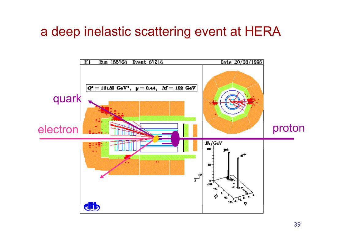
a deep inelastic scattering event at HERA
quark
electron proton
39
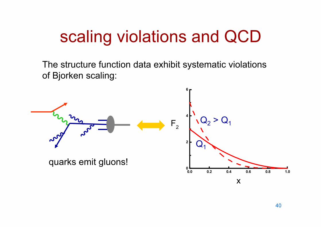
scaling violations and QCDscaling violations and QCDTh t t f ti d t hibit t ti i l tiThe structure function data exhibit systematic violations of Bjorken scaling:
6
4
F2Q2 > Q1
quarks emit gluons!
2 Q1
q g0.0 0.2 0.4 0.6 0.8 1.0
0
x
40

++++2
+2
+ …++ …+ +
where the logarithm comes from(‘collinear singularity’) and
then convolute with a ‘bare’ quark distribution in the proton:
q0(x)
p xp41

next, factorise the collinear divergence into a ‘renormalised’ quark distribution, by introducing the factorisation scale μ2 : q , y g μ
then finite, by construction
note arbitrariness of ‘factorisation scheme dependence’
we can choose C such that Cq= 0, the DIS scheme, or use dimensional _
q(x,μ2) is not calculable in perturbation theory,* but its scale (μ2)d d i
q
regularisation and remove the poles at N=4, the MS scheme, with Cq ≠ 0__
dependence is: DokshitzerGribovLipatovLipatovAltarelliParisi
*lattice QCD?42

note that we are free to choose μ2 = Q2 in which case
and thus the scaling violations of the structure function
coefficient function,see QCD book
… and thus the scaling violations of the structure function follow those of q(x,Q2) predicted by the DGLAP equation:
6
4
6
F 2
Q2 > Q1
q
0.0 0.2 0.4 0.6 0.8 1.00
2 Q1
q
x
the rate of change of F2 is proportional to αS(DGLAP) hence structure function data can be(DGLAP), hence structure function data can be used to measure the strong coupling!
43

however, we must also includethe gluon contributiong
coefficient functions- see QCD book
… and with additional terms in the DGLAP equations
splittingfunctions
note that at small (large) x, the gluon (quark) contributiongluon (quark) contribution dominates the evolution of the quark distributions, and thereforequark distributions, and therefore of F2 44

45
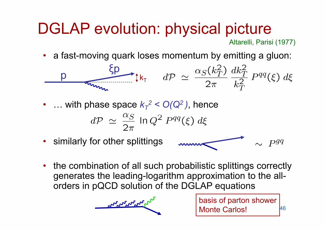
DGLAP evolution: physical picturep y p• a fast-moving quark loses momentum by emitting a gluon:
Altarelli, Parisi (1977)
kTp ξp
• … with phase space kT2 < O(Q2 ), hence
• similarly for other splittings• similarly for other splittings
• the combination of all such probabilistic splittings correctlythe combination of all such probabilistic splittings correctly generates the leading-logarithm approximation to the all-orders in pQCD solution of the DGLAP equations
basis of parton shower Monte Carlos! 46

beyond lowest order in pQCDgoing to higher orders in pQCD is straightforward in p gprinciple, since the above structure for F2 and for DGLAP li iDGLAP generalises in a straightforward way:
1972-77 1977-80 2004
see above see book very complicated!
The calculation of the complete set of P(2) splitting functions by Moch, Vermaseren and Vogt (hep-ph/0403192,0404111) completes the calculational
y p
g ( p p , ) ptools for a consistent NNLO pQCD treatment of Tevatron & LHC hard-scattering cross sections! 47

• and for the structure functions…
… where up to and including the O(αS3) coefficient
functions are known
• terminology:– LO: P(0)
– NLO: P(0,1) and C(1)
– NNLO: P(0,1,2) and C(1,2)
• the more pQCD orders are included, the weaker the dependence on the (unphysical) factorisation scale, μF
2
– and also the (unphysical) renormalisation scale, μR2 ; note above has μR
2 = Q2
48

parton distribution functions (again)
th b lk f th i f ti df f fitti DIS
parton distribution functions (again)
• the bulk of the information on pdfs comes from fitting DIS structure function data, although hadron-hadron collisions data also provide important constraints (see below)p p ( )
• pdfs are useful in two ways:p y– they are essential for predicting hadron collider cross sections, e.g.
Hp p
– they give us detailed information on the quark flavour content of the
Hp p
nucleon
49

how pdfs are obtained*p• choose a factorisation scheme (e.g. MSbar), an order in
perturbation theory (LO, NLO, NNLO) and a ‘starting p y ( , , ) gscale’ Q0 where pQCD applies (e.g. 1-2 GeV)
• parametrise the quark and gluon distributions at Q0,, e.g.
• l DGLAP ti t bt i th df t d• solve DGLAP equations to obtain the pdfs at any x and scale Q > Q0 ; fit data for parameters {Ai,ai, …αS}
• approximate the exact solutions (e g interpolation gridsapproximate the exact solutions (e.g. interpolation grids, expansions in polynomials etc) for ease of use; thus the output ‘global fits’ are available ‘off the shelf”, e.g.
i t | t tSUBROUTINE PDF(X,Q,U,UBAR,D,DBAR,…,BBAR,GLU)
input | output50*traditional method
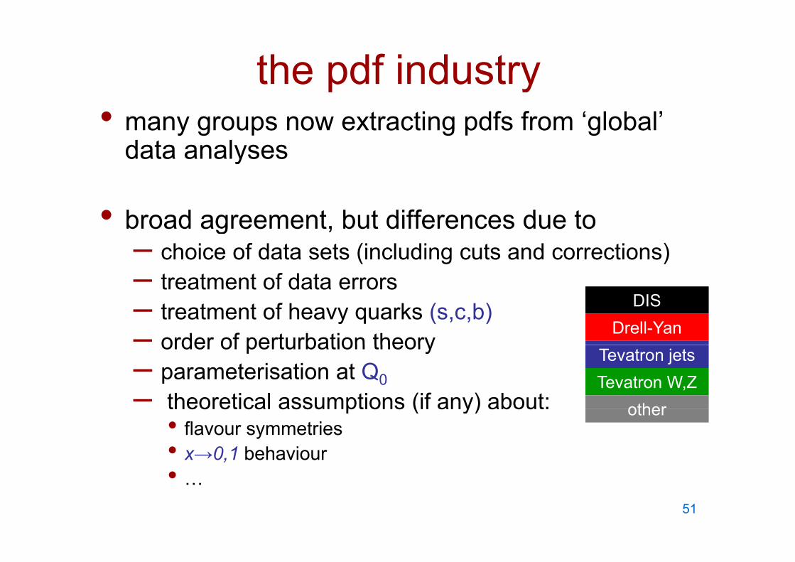
the pdf industryp y• many groups now extracting pdfs from ‘global’
data analysesdata analyses
• broad agreement but differences due to• broad agreement, but differences due to– choice of data sets (including cuts and corrections)– treatment of data errors– treatment of data errors– treatment of heavy quarks (s,c,b)– order of perturbation theory
DISDrell-Yan
order of perturbation theory– parameterisation at Q0– theoretical assumptions (if any) about:
Tevatron jetsTevatron W,Z
othertheoretical assumptions (if any) about: • flavour symmetries• x→0,1 behaviour•
other
• …51

recent global or quasi-global pdf fits
pdfs authors arXiv
ABKM S. Alekhin, J. Blümlein, S. Klein, S. Moch, and others
1007.3657, 0908.3128, 0908.2766, …
H.-L. Lai, M. Guzzi, J. Huston, Z. 1007.2241, 1004.4624, CTEQ
, , ,Li, P. Nadolsky, J. Pumplin, C.-P. Yuan, and others
, ,0910.4183, 0904.2424, 0802.0007, …
G M Glück P Jimenez-Delgado E 0909 1711 0810 4274GJR M. Glück, P. Jimenez Delgado, E. Reya, and others
0909.1711, 0810.4274, …
HERAPDF H1 and ZEUS collaborations 1006.4471, 0906.1108, …
MSTW A.D. Martin, W.J. Stirling, R.S. Thorne, G. Watt
1006.2753, 0905.3531, 0901.0002, …
NNPDFR. Ball, L. Del Debbio, S. Forte, A. Guffanti, J. Latorre, J. Rojo, M. Ubiali, and others
1005.0397, 1002.4407, 0912.2276, 0906.1958, …
52

MSTW08 CTEQ6.6X NNPDF2.0 HERAPDF1.0 ABKM09X GJR08
HERA DIS * *
F-T DIS F-T DIS
F-T DY
TEV W,Z +
TEV jets + j
GM-VFNS
NNLO + Run 1 only
* includes new combined H1-ZEUS data few% increase in quarks at low xX new (July 2010) ABKM and CTEQ updates: ABKM includes new combined H1-ZEUS data + new small-x parametrisation + partial NNLO HQ corrections; CT10
i l d bi d H1 ZEUS d R 2 j d d d lincludes new combined H1-ZEUS data + Run 2 jet data + extended gluon parametrisation + … more like MSTW08 53
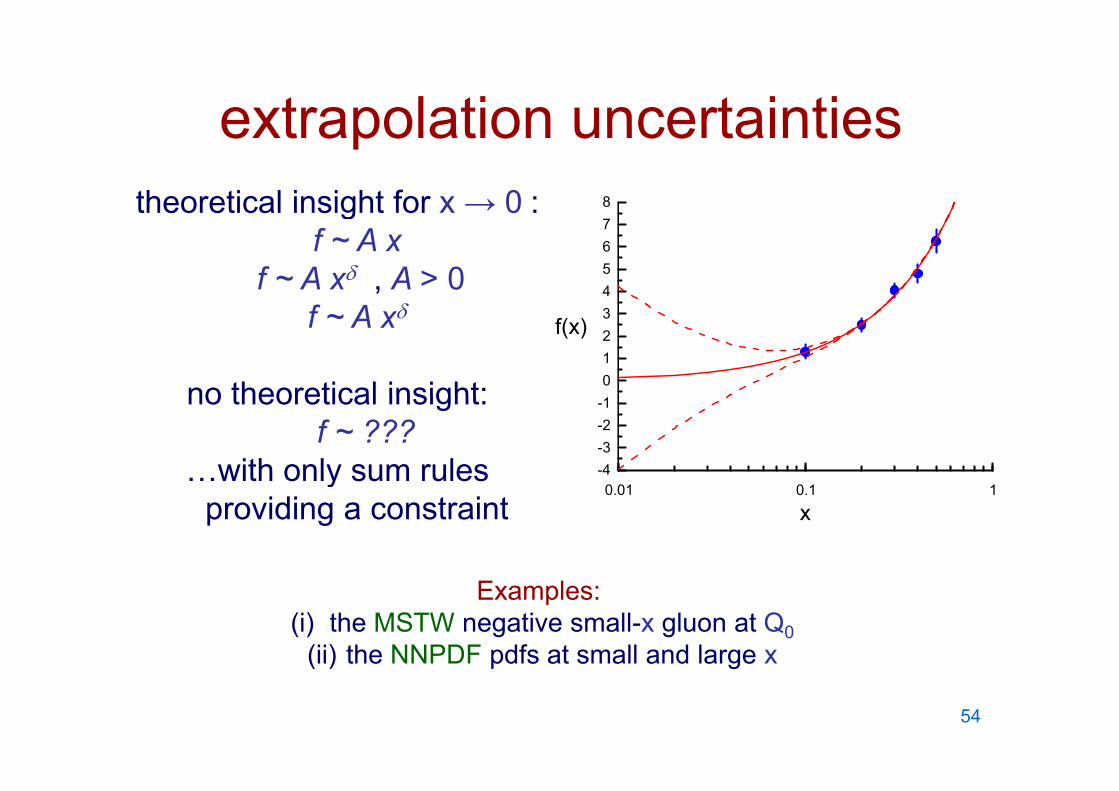
extrapolation uncertainties8
extrapolation uncertaintiestheoretical insight for x → 0 :
4567
gf ~ A x
f ~ A x , A > 0f A
0123
f(x)f ~ A x
no theoretical insight:
0 01 0 1 1-4-3-2-1no theoretical insight:
f ~ ???…with only sum rules
0.01 0.1 1
x
yproviding a constraint
Examples:(i) the MSTW negative small-x gluon at Q0
(ii) the NNPDF pdfs at small and large x( ) p g
54

summary of DIS datasummary of DIS data
+ neutrino FT DIS
data Note: must impose cutsdata Note: must impose cuts on DIS data to ensure validity of leading-twist DGLAP f li iDGLAP formalism in
analyses to determine pdfs, typically:p , yp y
Q2 > 2 - 4 GeV2
W2 = (1-x)/x Q2 > 10 - 15 GeV2
55

examples of data sets used in fits*
*MSTW2008 56

testing QCDtesting QCD
• i i t t f QCDstructure function data • precision test of QCD
• measurement of the strong coupling:
from H1, BCDMS, NMC
coupling:
NNLO(M ) 0 117 ± 0 003SNNLO(MZ) = 0.117 ± 0.003
(MSTW 2008 from global fit)DGLAP fit
(MSTW 2008, from global fit)
57
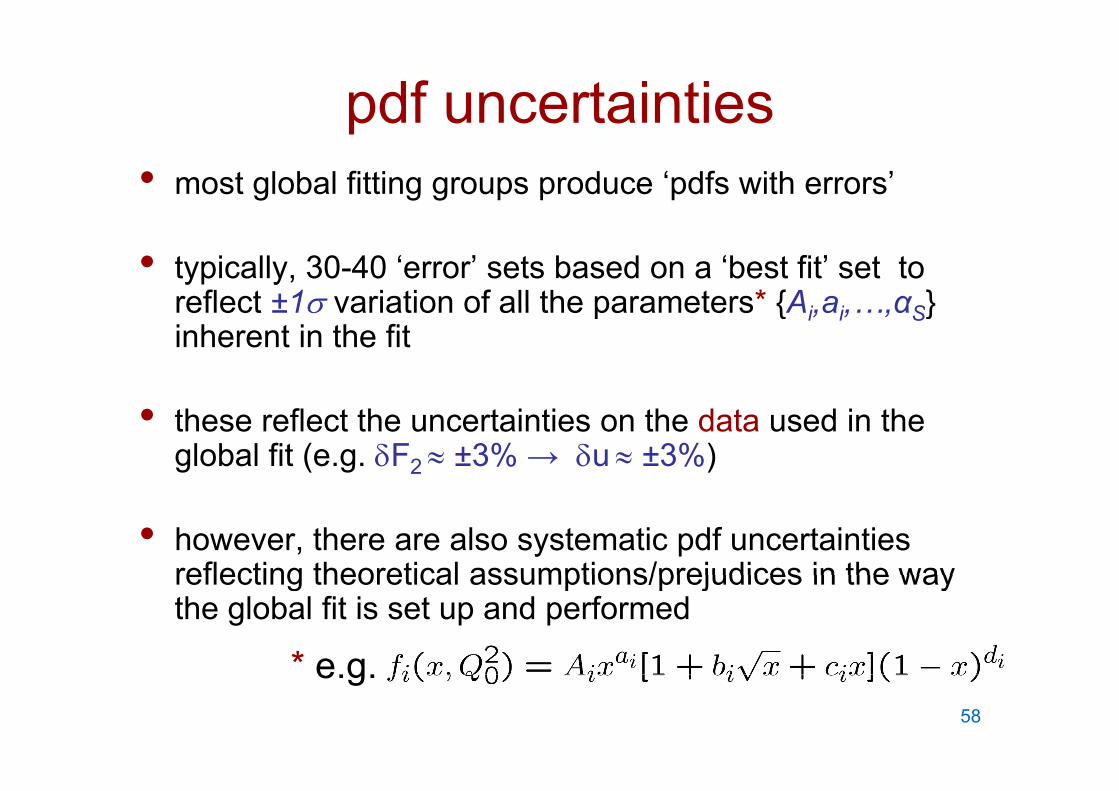
pdf uncertaintiesp• most global fitting groups produce ‘pdfs with errors’
• typically, 30-40 ‘error’ sets based on a ‘best fit’ set to reflect ±1 variation of all the parameters* {Ai ai αS}reflect ±1 variation of all the parameters {Ai,ai,…,αS}inherent in the fit
• these reflect the uncertainties on the data used in the global fit (e.g. F2 ±3% → u ±3%)
• however, there are also systematic pdf uncertainties reflecting theoretical assumptions/prejudices in the wayreflecting theoretical assumptions/prejudices in the way the global fit is set up and performed
* e g e.g.58

59

60

MSTW2008(NLO) vs. CTEQ6.6
Note:
CTEQ error bands comparable with MSTW 90%cl set (different % (definition of tolerance)
CTEQ light quarks and g qgluons slightly larger at small x because of imposition of positivity on gluon at Q0
2
61

where to find parton distributions
HEPDATA pdf websiteHEPDATA pdf websitehttp://hepdata.cedar.acuk/pdfs.uk/pdfs
• access to code for• access to code for MSTW, CTEQ,NNPDFetcetc
• online pdf plottingonline pdf plotting
• also LHAPDF interfacealso LHAPDF interface62

Scattering processes at high energy
What can we calculate?
Scattering processes at high energy hadron colliders can be classified as either HARD or SOFT
Quantum Chromodynamics (QCD) is the underlying theory for all such processes, but the approach (and the p , pp (level of understanding) is very different for the two cases
For HARD processes, e.g. W or high-ET jet production, the rates and event properties can be predicted with some precision using perturbation theory
For SOFT processes, e.g. the total ffcross section or diffractive processes,
the rates and properties are dominated by non-perturbative QCD effects, which
h l ll d t dare much less well understood
63

hard scattering in hadron-hadron collisions
higher-order pQCD corrections; i di ti j t
paccompanying radiation, jets
parton distribution X = W, Z, top, jets,d st but ofunctions
, , p, j ,SUSY, H, …
tuned event simulation (parton showers + UE) MCs, interfaced with LO or NLO hard scattering MEs
p
for inclusive production, the basic calculational framework is provided by the QCD FACTORISATION THEOREM:
64

kinematics
proton proton
x1P
p
x2P
pM
• collision energy:
• parton momenta:• parton momenta:
• invariant mass:
• rapidity:
65
x P
proton
x P
protonM
x1P x2P
DGLAP evolution
66

early history: the Drell-Yan processearly history: the Drell Yan process
+
*quark
antiquark
= M2/s
-antiquark
“The full range of processes of the type A + B → (nowadays) … and to study the g p yp+- + X with incident p,, K, etc affords the interesting possibility of comparing their parton and antiparton structures” (Drell and Yan, 1970)
( y ) yscattering of quarks and gluons, and how such scattering creates new particlesp ( ) p
67

jets! (1981)
jet
antiprotone.g. two gluons scattering at
jet
antiprotonproton
gwide angle
68
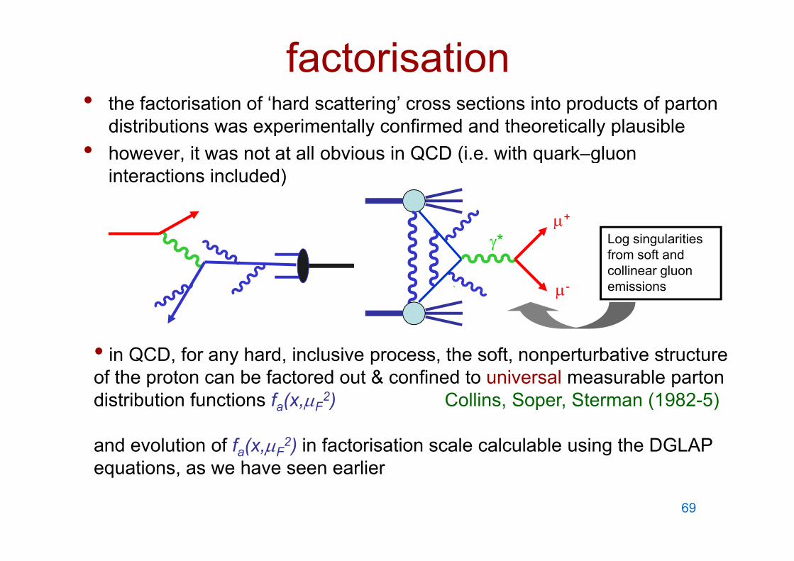
factorisation• the factorisation of ‘hard scattering’ cross sections into products of parton
distributions was experimentally confirmed and theoretically plausible• however it was not at all obvious in QCD (i e with quark gluonhowever, it was not at all obvious in QCD (i.e. with quark–gluon
interactions included)
++
* Log singularities from soft and collinear gluon
- emissions
• in QCD, for any hard, inclusive process, the soft, nonperturbative structure of the proton can be factored out & confined to universal measurable parton distribution functions fa(x,F
2) Collins, Soper, Sterman (1982-5)a( ,F ) , p , ( )
and evolution of fa(x,F2) in factorisation scale calculable using the DGLAP
equations as we have seen earlierequations, as we have seen earlier
69

Drell Yan as a probe of new physicsDrell-Yan as a probe of new physicsLarge Extra Dimension (and other New Physics) models have new resonances that could contribute to Drell-Yan
+
-
G
need to understand the SM contribution to high precision!
CDF Run II (2009)
70

Summary: the QCD factorization theorem for hard-scattering (short-distance) inclusive processes
where X=W, Z, H, high-ET jets, SUSY sparticles, black hole, …, and Q is the ‘hard scale’ (e.g. = MX), usually F = R = Q, and is known … ^( g X) y F R
• to some fixed order in pQCD, e.g. high-ET jets
• or in some leading logarithm approximation (LL NLL ) to all orders via resummation
(LL, NLL, …) to all orders via resummation
71

hard scattering cross section master formula
a 1• i t fi l t t i
.
.
.
a 2b n
• impose cuts on final state energies, angles, etc. as required
• 2 ? You choose!
• maximum 3n-2 integrations (fewer formaximum 3n 2 integrations (fewer for differential distributions); in practice, generally use Monte Carlo techniques
72

parton luminosity functions• a quick and easy way to assess the mass, collider
energy and pdf dependence of production cross sectionsgy p p p
as X
a
b
• i ll th d d d i t i d• i.e. all the mass and energy dependence is contained in the X-independent parton luminosity function in [ ]• useful combinations areuseful combinations are • and also useful for assessing the uncertainty on cross sections due to uncertainties in the pdfs (see later)p ( )
73

SSVS
more such luminosity plots available at www.hep.phy.cam.ac.uk/~wjs/plots/plots.html74

75

e.g.ggHggH
qqVHqqqqH
76

3QCD at LHCQCD at LHC
• leading-order calculationsg
• beyond leading order: higher-order perturbative QCD corrections
• benchmark cross sections
• beyond perturbation theory
77
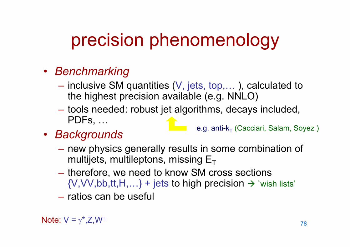
precision phenomenologyprecision phenomenologyB h ki• Benchmarking– inclusive SM quantities (V, jets, top,… ), calculated to
the highest precision available (e g NNLO)the highest precision available (e.g. NNLO)– tools needed: robust jet algorithms, decays included,
PDFs, …,• Backgrounds
– new physics generally results in some combination of
e.g. anti-kT (Cacciari, Salam, Soyez )
new physics generally results in some combination of multijets, multileptons, missing ET
– therefore, we need to know SM cross sections {V VV bb tt H } j t t hi h i i{V,VV,bb,tt,H,…} + jets to high precision `wish lists’
– ratios can be useful
Note: V = *,Z,W78

how precise?p• LO for generic PS Monte Carlos, tree-
level MEs
• NLO for NLO-MCs and many parton-level signal and background processes – in principle less sensitivity to– in principle, less sensitivity to
unphysical renormalisation and factorisation scales, μR and μF– parton merging to give structure in jetsmore types of incoming partons– more types of incoming partons
– more reliable pdfs– better description of final state
kinematics
• NNLO for a limited number of ‘precision observables’ (W, Z, DY, H, …)
+ E/W corrections, resummed HO terms etc…
th = UHO pdf param …79

emerging ‘precision’ phenomenology at LHCW, Z production
jet production
80

survey of pQCD calculations• focus first on fixed-order calculations:
d = A({P}) α (2) N [ 1 + C ({P} 2) α (2) + C ({P} 2) α (2) 2 + ]d = A({P}) αS (2) N [ 1 + C1({P}, 2) αS (2) + C2({P},2) αS (2) 2 + …. ]
… where {P} refers to the kinematic variables for the particular process. For hadron colliders there will also be pdfs and dependence on the factorisation scalecolliders there will also be pdfs and dependence on the factorisation scale.
• thus LO (A only), NLO (A, C1 only), NNLO (A,C1,C2 only) etc,
• note that in some cases the coefficients may contain large logarithms L of ratios of kinematic variables, and it may be possible to identify and resum these to all orders using a leading log approximation, e.g.orders using a leading log approximation, e.g.
d = A αSN [ 1 + (c11 L + c10 ) αS + (c22 L2 + c21 L + c20 ) αS
2 + …. ]~ A αS
N exp(c11 L αS + c21 L αS2) [ 1 + c10 αS + c20 αS
2 + ] A αS exp(c11 L αS + c21 L αS ) [ 1 + c10 αS + c20 αS + …. ]
where e.g. L = log(M/qT), log(1/x), log(1-T), … >> 1, thus LL, NLL, NNLL, etc.
81
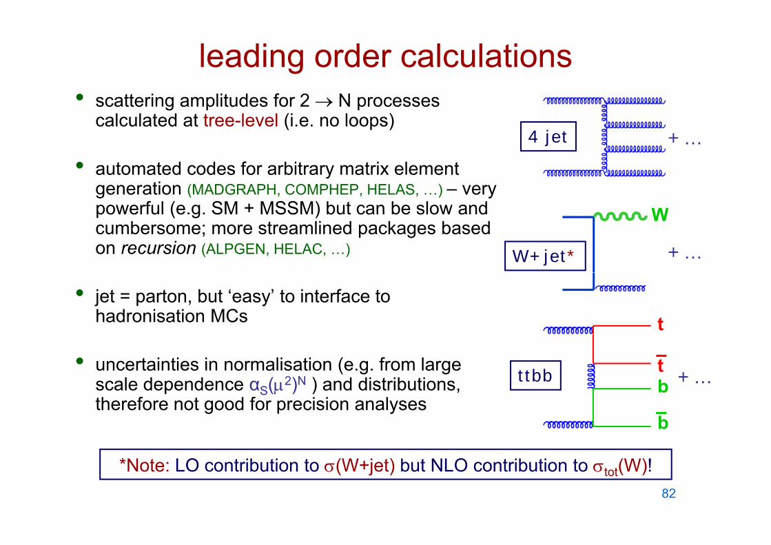
leading order calculations• scattering amplitudes for 2 N processes
calculated at tree-level (i.e. no loops) 4 jet +…
• automated codes for arbitrary matrix element generation (MADGRAPH, COMPHEP, HELAS, …) – very powerful (e g SM + MSSM) but can be slow and Wpowerful (e.g. SM + MSSM) but can be slow and cumbersome; more streamlined packages based on recursion (ALPGEN, HELAC, …)
W
W+jet* +…
• jet = parton, but ‘easy’ to interface to hadronisation MCs t
• uncertainties in normalisation (e.g. from large scale dependence αS(2)N ) and distributions,
tbttbb +…
therefore not good for precision analysesb
*Note: LO contribution to (W+jet) but NLO contribution to tot(W)!82

htt // l h h/ l / l /http://mlm.home.cern.ch/mlm/alpgen/
83

next-to-leading order calculations• the NLO contributions correspond to an additional real
gluon in final state and a virtual gluon in loop correction, i.e. (N) (N 1)dV(N) + dR
(N+1) for a 2 N process at LO, e.g.
+2
+++ +2
+2
+++ +2
+2
• the LO prediction is stabilised, in particular by reducing the (renormalisation and factorisation) scale dependence(renormalisation and factorisation) scale dependence
• jet structure begins to emerge• much recent progress (see below)uc ece t p og ess (see be o )• ... and now can interface with parton shower MC (e.g.
MC@NLO)• the NLO corrections are now known for ‘most’ processes of
interest
84

recent developments at NLOrecent developments at NLO• traditional methods based on Feynman diagrams, then reduction to
known (scalar box triangle bubble and tadpole) integralsknown (scalar box, triangle, bubble and tadpole) integrals
• … and new methods based on unitarity and on-shell recursion: assemble loop diagrams from individual tree level diagramsassemble loop-diagrams from individual tree-level diagrams– basic idea: Bern, Dixon, Kosower 1993– cuts with respect to on-shell complex loop momenta:
Cachazo Britto Feng 2004Cachazo, Britto, Feng 2004– tensor reduction scheme: Ossola, Pittau, Papadopoulos 2006– integrating the OPP procedure with unitarity: Ellis, Giele, Kunszt 2008– D-dimensional unitarity: Giele, Kunszt, Melnikov 2008D dimensional unitarity: Giele, Kunszt, Melnikov 2008– …
• … and the appearance of automated programmes for one-loop,… and the appearance of automated programmes for one loop, multi-leg amplitudes, either based on – traditional or numerical Feynman approaches (Golem, …)– unitarity/recursion (BlackHat, CutTools, Rocket, …)
85

recent NLO results…*• pp W+3j [Rocket: Ellis, Melnikov & Zanderighi] [unitarity]• pp W+3j [BlackHat: Berger et al] [unitarity]• pp tt bb [Bredenstein et al] [traditional]• pp tt bb [HELAC-NLO: Bevilacqua et al] [unitarity]• pp qq 4b [Golem: Binoth et al] [traditional]• pp tt+2j [HELAC-NLO: Bevilacqua et al] [unitarity]• pp Z+3j [BlackHat: Berger et al] [unitarity]• pp W+4j [BlackHat: Berger et al, partial] [unitarity]• …
with earlier results on V,H + 2 jets, VV,tt + 1 jet, VVV, ttH, ttZ, …
*In contrast, for NNLO we still only have inclusive *,W,Z,H with rapidity distributions and decays (although much progress on top, single jet, …)
86*relevant for LHC

calculation time: one-loop pure gluon amplitudes
Giele and Zanderighi, 2008
loop
tree
87

general structure of a QCD perturbation seriesrecall
general structure of a QCD perturbation series• choose a renormalisation scheme (e.g. MSbar)• calculate cross section to some order (e g NLO)calculate cross section to some order (e.g. NLO)
physical process dependent coefficients renormalisation
• note d/d=0 “to all orders” but in practice
p yvariable(s)
p pdepending on P scale
note d/d 0 to all orders , but in practiced(N+n)/d= O((N+n)S
N+n+1)
• can try to help convergence by using a “physical scale choice”, ~ P , e.g. = MZ or = ET
jet
• what if there is a wide range of P’s in the process, e.g. W + n jets? 88

K. Ellis
Top at Tevatron
K. Ellis
Bottom at LHC
t NLO!
89
reason: new processes open up at NLO!

in complicated processes like W + n jets, there are often many ‘reasonable’ choices of scales:often many reasonable choices of scales:
‘blended’ scales like HT can seamlessly take t f diff t ki ti l fi tiaccount of different kinematical configurations:
Berger et al., arXiv:0907.1984

LHC benchmark cross sections
91

parton luminosity comparisonsRun 1 vs. Run 2 Tevatron jet data
positivity constraint on input gluon
No Tevatron jet data or FT DISdata or FT-DIS data in fit
momentum sum ruleZM-VFNS
92
Luminosity and cross section plots from Graeme Watt, available at projects.hepforge.org/mstwpdf/pdf4lhc

more restricted parametrisation
Tevatron jet data not in fit
93

new combined HERA SF data
ZM-VFNS
94
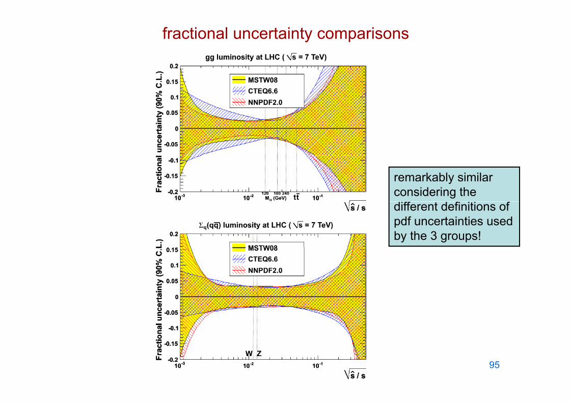
fractional uncertainty comparisons
remarkably similar considering the different definitions of pdf uncertainties used by the 3 groups!
95

NLO and NNLO parton luminosity comparisons
96

differences probably due to sea quark
benchmark W,Z cross sectionsq
flavour structure
97
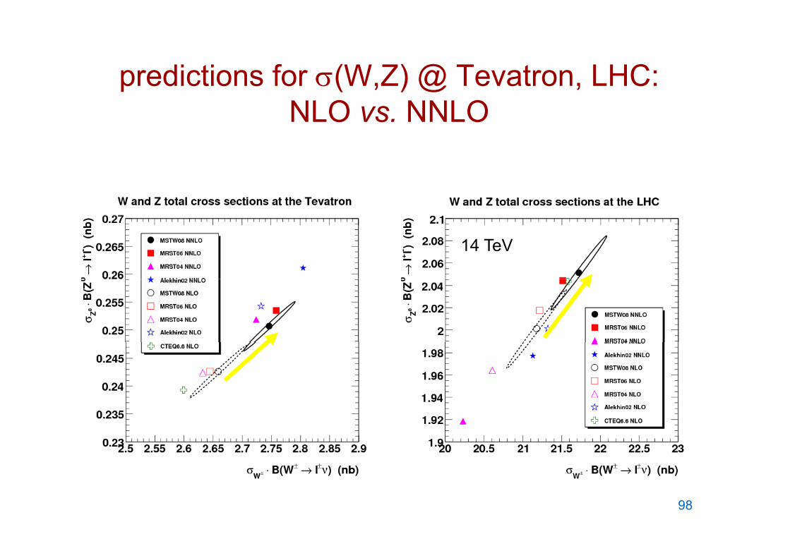
predictions for (W,Z) @ Tevatron, LHC:p ( , ) @ ,NLO vs. NNLO
14 TeV
98

impact of sea quarks on the NLO W charge asymmetry ratio at 7 TeV:
pdfs R(W+/W-){udg} only 1 53{udg} only 1.53{udscbg} = MSTW08 1.42 0.02{udscbg}sea only 0.99{ g}sea y{udscbg}sym.sea only 1.00
99
at LHC, ~30% of W and Z total cross sections involves s,c,b quarks

using the W+- charge asymmetry at the LHC• at the Tevatron (W+) = (W–), whereas at LHC (W+) ~ (1.4 –
1.3) (W–)
• can use this asymmetry to calibrate backgrounds to new physics, since typically NP(X → W+ + …) = NP(X → W– + …)
• example:
in this case
whereas…
which can in principle help distinguish signal and background100

C.H. Kom & WJS, arXiv:1004.3404
R increases with jet pT
min
R larger at 7 TeV LHC Berger et al (arXiv:1009.2338)- 7 TeV, slightly different cuts, g y

the impact of NNLO: W,Zp
Anastasiou, Dixon,Anastasiou, Dixon, Melnikov, Petriello, 2004
• l l i ti t i t h• only scale variation uncertainty shown• central values calculated for a fixed set pdfs with a fixed value of S(MZ
2)102

benchmark (NLO) Higgs cross sections
… differences from both pdfs AND S !103

104

How to define an overallHow to define an overall ‘best theory prediction’?! See
LHC Higgs Cross Section Working Group meeting, o g G oup ee g,
higgs2010.to.infn.it
Note: (i) for MSTW08, uncertainty band similar at NNLO(ii) everything here is at fixed scale =MH !
105

the impact of NNLO: H
Harlander,KilgoreAnastasiou, Melnikov
Ravindran, Smith, van Neerven…
• only scale variation uncertainty shown• l l l l d f fi d df i h fi d l f (M )• central values calculated for a fixed set pdfs with a fixed value of S(MZ)• the NNLO band is about 10%, or 15% if R and F varied independently106

scale variation in gg H?• ‘ i l’ h (NNLO)
scale variation in gg H?• ‘conventional’ approach (NNLO):
+10%- 10%
• ‘conservative’ approach (Baglio and Djouadi) , NNLO normalised to NNLL
+15%- 20%
• ‘radical approach’: N3LL (Ahrens, Becher, Neubert, Yang, 1008.3162)
+3%+3%- 3%
choice of scale and range – flat prior? 107
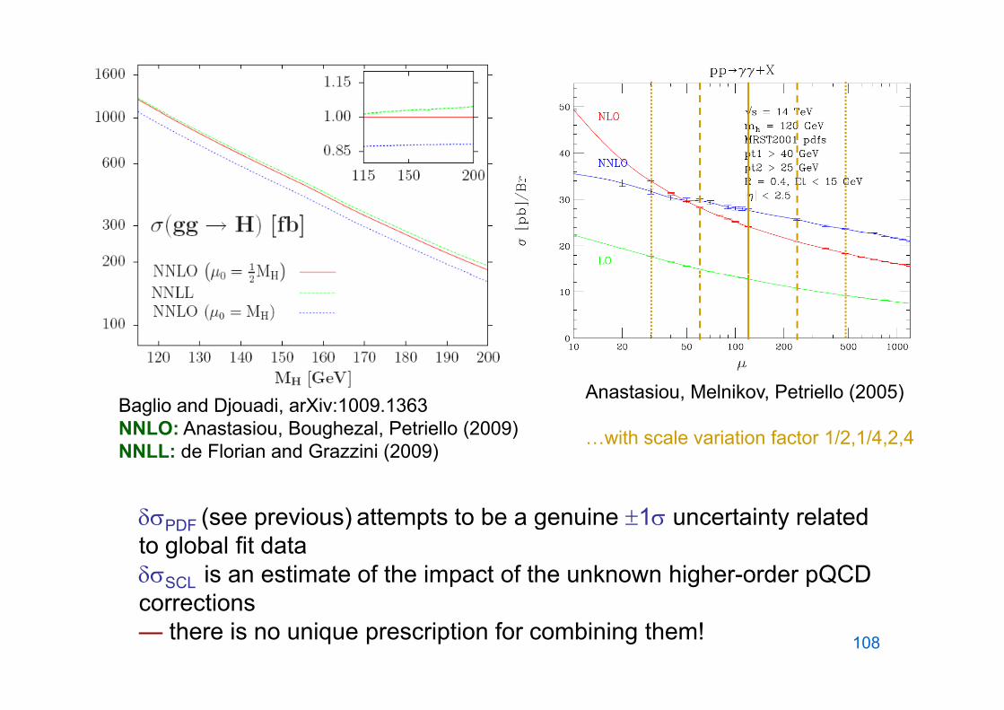
Baglio and Djouadi, arXiv:1009.1363NNLO: Anastasiou, Boughezal, Petriello (2009)
Anastasiou, Melnikov, Petriello (2005)
with scale variation factor 1/2 1/4 2 4, g , ( )NNLL: de Florian and Grazzini (2009)
(see previous) attempts to be a genuine 1 uncertainty related
…with scale variation factor 1/2,1/4,2,4
PDF (see previous) attempts to be a genuine 1 uncertainty related to global fit data SCL is an estimate of the impact of the unknown higher-order pQCD
ticorrections— there is no unique prescription for combining them! 108
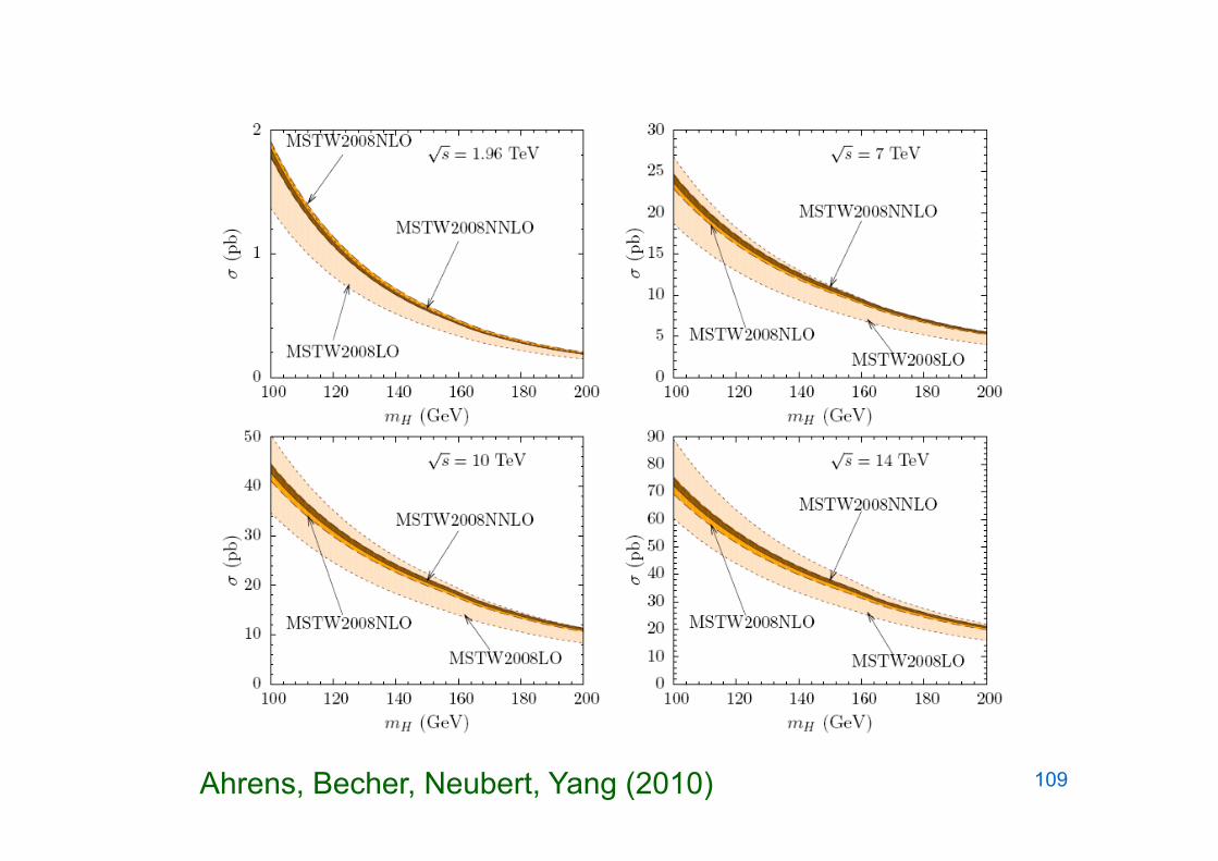
Ahrens, Becher, Neubert, Yang (2010) 109

SM Higgs: Tevatron exclusion limitsSM Higgs: Tevatron exclusion limits
theory ±50%
110

beyond perturbation theory
111

beyond perturbation theorynon-perturbative effects arise in many different ways• emission of gluons with kT < Q0 off ‘active’ partons • soft exchanges between partons of the same or different beamsoft exchanges between partons of the same or different beam
particlesmanifestations include…• h d tt i t t t t• hard scattering occurs at net non-zero transverse momentum• ‘underlying event’ additional hadronic energy
precision phenomenology requires a quantitative understanding of these effects! 112

‘intrinsic’ transverse momentumsimple parton model assumes partons have zero transverse momentum
… but data shows that the DY lepton pair is produced with non-zero <pT>
+113

the perturbative tail is even more apparent in W, Z production at the Tevatron, and can be well accounted for by the 2→2 yscattering processes:
… with known NLO pQCD corrections. Note that the pT distribution diverges as pT→0 due to soft gluon emission:
the O(αS) virtual gluon correction contributes at pT=0, in such a way as k h i d di ib i fi ito make the integrated distribution finite
intrinsic kT can also be included, by convoluting with the pQCD contribution114

resummation• when pT << M , the pQCD series contains large logarithms ln(M2/pT
2)at each order:
which spoils the convergence of the series when
• fortunately these logarithms can be resummed to all orders infortunately, these logarithms can be resummed to all orders in pQCD, to generate a Sudakov form factor:
… which regulates the LO singularity at pT = 0… which regulates the LO singularity at pT 0
• the effect of the form factor is (just about) visible in the (Tevatron) data(Tevatron) data
115

resummation contd Zresummation contd.KuleszaSterman
• theoretical refinements include the addition of sub-leading logarithms (e g NNLL)
StermanVogelsang
leading logarithms (e.g. NNLL) and nonperturbative contributions, and merging the
d t ib ti ith
qT (GeV)
resummed contributions with the fixed order (e.g. NLO) contributions appropriate for large pT
• the resummation formalism is also valid for Higgs production at LHC via gg→H
116

• comparison ofcomparison of resummed / fixed-order calculations for Higgs (MH= 125 GeV) p distribution= 125 GeV) pT distribution at LHC
B l t l h h/0403052Balazs et al, hep-ph/0403052
• differences due mainly t diff t NnLO dto different NnLO and NnLL contributions included
• Tevatron d(Z)/dpTprovides good test of calculations
117

full event simulation at hadron colliders• it is important (designing detectors,
interpreting events, etc.) to have a good d t di f ll f t f th lli iunderstanding of all features of the collisions
– not just the ‘hard scattering’ part • this is very difficult because our
understanding of the non-perturbative part of QCD is still quite primitive
• at present, therefore, we have to resort to p , ,models (PYTHIA, HERWIG, …) …
118

Monte Carlo Event GeneratorsMonte Carlo Event Generators• programs that simulates particle physics events with theprograms that simulates particle physics events with the
same probability as they occur in nature• widely used for signal and background estimatesy g g• the main programs in current use are PYTHIA and HERWIG• the simulation comprises different phases:
– start by simulating a hard scattering process – the fundamental interaction (usually a 2→2 process but could be more complicated for particular signal/background processes)
– this is followed by the simulation of (soft and collinear) QCD radiation using a parton shower algorithm
– non-perturbative models are then used to simulate the hadronizationnon perturbative models are then used to simulate the hadronization of the quarks and gluons into the observed hadrons and the underlying event
119

a Monte Carlo eventa Monte Carlo event
Hard Perturbative scattering:Hard Perturbative scattering:
Usually calculated at leading order in QCD, electroweak theory or some BSM model.Modelling of the
soft underlying event
Multiple perturbative scattering.
event
P t b ti DInitial and Final State parton showers resum the large QCD logs.
Perturbative Decays calculated in QCD, EW or some BSM theory.Non-perturbative modelling of the
Finally the unstable hadrons are decayed.
hadronization process.y
from Peter Richardson (HERWIG)120

(hadron collider) processes in HERWIG
from Peter Richardson121

however …however …• the tuning of the nonperturbative parts of the models is
performed at a single collider energy (or limited range ofperformed at a single collider energy (or limited range of energies) – can we trust the extrapolation to LHC?!
• in general the event generators only use leading order matrix elements and therefore the normalisation ismatrix elements and therefore the normalisation is uncertain
• this can be overcome by renormalising to known NLO y getc results or by incorporating next-to-leading order matrix elements (real + virtual emissions) – see below
• only soft and collinear emission is accounted for in theonly soft and collinear emission is accounted for in the parton shower, therefore the emission of additional hard, high ET jets is generally significantly underestimated
• for this reason it is possible that many of the previous• for this reason, it is possible that many of the previous LHC studies of new physics signals have significantly underestimated the Standard Model backgrounds
122

123

interfacing NnLO and parton showers
++
Benefits of both:e e s o bo
NnLO correct overall rate, hard scattering kinematics, reduced scale dep.PS complete event picture correct treatment of collinear logs to all ordersPS complete event picture, correct treatment of collinear logs to all orders
Example: MC@NLO Frixione, Webber, Nason,www.hep.phy.cam.ac.uk/theory/webber/MCatNLO/
processes include …pp WW,WZ,ZZ,bb,tt,H0,W,Z/, ...
pT distribution of tt at Tevatron 124

summary• QCD: non-abelian gauge field theory for the strong
interaction and essential component of the Standard 2Model; symmetry = SU(3) and S(MZ2) = 0.118 ± 0.001
• th k t 40 th ti l t di t d b• thanks to ~ 40 years theoretical studies, supported by experimental measurements, we now know how to calculate (an important class of) proton-proton collider ( p ) p pevent rates reliably and with a high precision
• the key ingredients are the factorisation theorem and the universal parton distribution functions
• such calculations underpin searches (at the Tevatronand the LHC) for Higgs, SUSY, etcand the LHC) for Higgs, SUSY, etc
125

summary contd.• …but much work still needs to be done, in particular:
l l ti d NNLO QCD– calculating more and more NNLO pQCDcorrections (and some missing NLO ones too)
– better understanding of ‘scale dependence’– better understanding of scale dependence– further refining the pdfs, and understanding their
uncertaintiesuncertainties– understanding the detailed event structure, which
is outside the domain of pQCD and is currentlyis outside the domain of pQCD and is currently simply modelled
– extending the calculations to new types of g ypproduction processes, e.g. central exclusive diffractive production, double parton scattering, ...
126

extra slidesextra slides
127

anatomy of a NNLO calculation: p + p jet + Xanatomy of a NNLO calculation: p + p jet + X
• 2 loop, 2 parton final statep p
• | 1 loop |2, 2 parton final state
• 1 loop, 3 parton final states or 2 +1 final stateor 2 +1 final state
• tree, 4 parton final states soft, collinear
por 3 + 1 parton final states or 2 + 2 parton final state
the collinear and soft singularities exactly cancel between the N +1 and N + 1 loop contributionsbetween the N +1 and N + 1-loop contributions
128
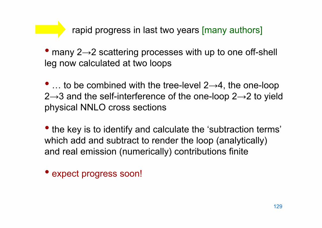
rapid progress in last two years [many authors]
• many 2→2 scattering processes with up to one off-shell leg now calculated at two loopsleg now calculated at two loops
• … to be combined with the tree-level 2→4, the one-loop… to be combined with the tree level 2 4, the one loop 2→3 and the self-interference of the one-loop 2→2 to yield physical NNLO cross sections
• the key is to identify and calculate the ‘subtraction terms’ which add and subtract to render the loop (analytically)which add and subtract to render the loop (analytically) and real emission (numerically) contributions finite
• expect progress soon!
129
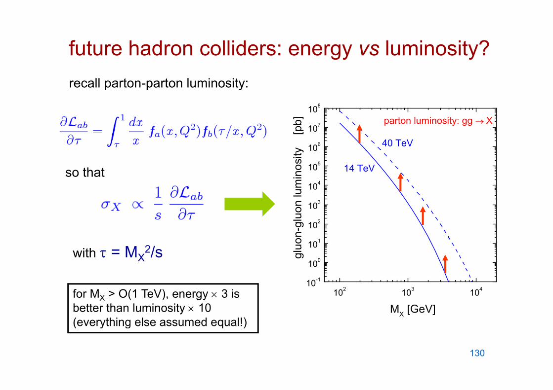
future hadron colliders: energy vs luminosity?
108
recall parton-parton luminosity:
106
107
108
40 TeV
parton luminosity: gg X
y
[pb]
104
105
10
14 TeV
umin
osity
so that
1
102
103
on-g
luon
l10-1
100
101
gluowith = MX2/s
102 103 10410
MX [GeV]for MX > O(1 TeV), energy 3 is better than luminosity 10 (everything else assumed equal!)( y g q )
130