1

Oct. 12, 2005

QM/MM: What have we learned, where are we, and where

do we go from here?

Hai Lin1,2 and Donald G. Truhlar1

(1) Chemistry Department and Supercomputing Institute, University of Minnesota, 207

Pleasant Street SE, Minneapolis, Minnesota 55455-0431

(2) Chemistry Department, University of Colorado at Denver, PO Box 173364, Denver,

CO 80217

Contribution to the Proceedings of the 10th Electronic Computational Chemistry

Conference, to be published in Theoretical Chemistry Accounts.

Correspondence to: Hai Lin, Donald G. Truhlar

e-mail: hai.lin@cudenver.edu, truhlar@umn.edu

2

Abstract. This paper briefly reviews the current status of the most popular methods

for combined quantum mechanical/molecular mechanical (QM/MM) calculations,

including their advantages and disadvantages. There is a special emphasis on very

general link atom methods and various ways to treat the charge near the boundary.

Mechanical and electric embedding are contrasted. We consider methods applicable

to gas-phase organic chemistry, liquid-phase organic and organometallic chemistry,

biochemistry, and solid-state chemistry. Then we review some recent tests of

QM/MM methods and summarize what we learn about QM/MM from these

studies. We also discuss some available software. Finally, we present a few

comments about future directions of research in this exciting area, where we focus

on more intimate bleeds of QM with MM.

Keywords: Boundary Treatment – Combined QM/MM – Electrostatic Interactions

– Embedding Scheme – Link Atom – Multi-configuration Molecular Mechanics –

Potential Energy Surfaces

3

I. Introduction

Despite of the increasing computational capability now available, molecular modeling

and simulation of large, complex systems at the atomic level remains a challenge to

computational chemists. At the same time, there is increasing interest in nanostructured

materials, condensed-phase reactions, and catalytic systems, including designer zeolites

and enzymes, and in modeling systems over longer time scales that reveal new

mechanistic details. The central problem is: can we efficiently accomplish accurate

calculations for large reactive systems over long time scales? As usual, we require

advances in modeling potential energy surfaces, in statistical mechanical sampling, and in

dynamics. The present article is concerned with the potentials.

Models based on classical mechanical constructs such as molecular mechanical (MM)

force fields that are based on empirical potentials describing small-amplitude vibrations,

torsions, van der Waals interactions, and electrostatic interactions have been widely used

in molecular dynamics (MD) simulations of large and complex organic and biological

systems1-25 as well as inorganic and solid-state systems.26-31 However, the MM force

fields are unable to describe the changes in the electronic structure of a system

undergoing a chemical reaction. Such changes in electronic structure in processes that

involve bond-breaking and bond-forming, charge transfer, and/or electronic excitation,

require quantum mechanics (QM) for a proper treatment. However, due to the very

demanding computational cost, the application of QM is still limited to relatively small

systems consisting of up to tens or several hundreds of atoms, or even smaller systems

when the highest levels of theory are employed.

Algorithms that combine quantum mechanics and molecular mechanics provide a

solution to this problem. These algorithms in principle combine the accuracy of a

quantum mechanical description with the low computational cost of molecular

mechanics, and they have become popular in the past decades. The incorporation of

quantum mechanics into molecular mechanics can be accomplished in various ways, and

one of them is the so-called combined quantum mechanical and molecular mechanical

(QM/MM) methodology.32-151

4

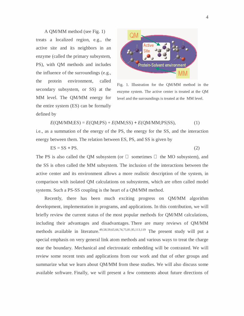
A QM/MM method (see Fig. 1)

treats a localized region, e.g., the

active site and its neighbors in an

enzyme (called the primary subsystem,

PS), with QM methods and includes

the influence of the surroundings (e.g.,

the protein environment, called

secondary subsystem, or SS) at the

MM level. The QM/MM energy for

the entire system (ES) can be formally

defined by

E(QM/MM;ES) = E(QM;PS) + E(MM;SS) + E(QM/MM;PS|SS), (1)

i.e., as a summation of the energy of the PS, the energy for the SS, and the interaction

energy between them. The relation between ES, PS, and SS is given by

ES = SS + PS. (2)

The PS is also called the QM subsystem (or sometimes the MO subsystem), and

the SS is often called the MM subsystem. The inclusion of the interactions between the

active center and its environment allows a more realistic description of the system, in

comparison with isolated QM calculations on subsystems, which are often called model

systems. Such a PS-SS coupling is the heart of a QM/MM method.

Recently, there has been much exciting progress on QM/MM algorithm

development, implementation in programs, and applications. In this contribution, we will

briefly review the current status of the most popular methods for QM/MM calculations,

including their advantages and disadvantages. There are many reviews of QM/MM

methods available in literature.49,58,59,65,66,74,75,81,95,113,119 The present study will put a

special emphasis on very general link atom methods and various ways to treat the charge

near the boundary. Mechanical and electrostatic embedding will be contrasted. We will

review some recent tests and applications from our work and that of other groups and

summarize what we learn about QM/MM from these studies. We will also discuss some

available software. Finally, we will present a few comments about future directions of

Fig. 1. Illustration for the QM/MM method in the

enzyme system. The active center is treated at the QM

level and the surroundings is treated at the MM level.

5

research in this exciting area. The applications of QM/MM methods are very interesting

and very important, but they are not emphasized in this review.

II. Interactions between the Primary and Secondary Subsystems

The coupling between the primary system (PS) and the secondary subsystem (SS) is

the heart of a QM/MM method. The coupling, in general, must be capable of treating

both bonded interactions (bond stretching, bond bending, and internal rotation,

sometimes called valence forces) and non-bonded interactions (electrostatic interaction

and van der Waals interactions). Various QM/MM schemes have been developed to treat

the interactions between the PS and SS.

As might be expected from its general importance in a myriad of contexts,152 the

electrostatic interaction is the key element of the coupling. Depending on the treatment of

the electrostatic interaction between the PS and SS, the QM/MM schemes can be divided

into two groups, the group of mechanical embedding and the group of electric

embedding.44 A mechanical embedding (ME) scheme performs QM computations for the

PS in the absence of the SS, and treats the interactions between the PS and SS at the MM

level. These interactions usually include both bonded (stretching, bending, and torsional)

interactions and non-bonded (electrostatic and van der Waals) interactions. The original

integrated molecular-orbital molecular-mechanics (IMOMM) scheme39,52,62 by

Morokuma and coworkers, which is also known as the two-layer ONIOM(MO:MM)

method, is an ME scheme.

In an electrostatic embedding (EE) scheme, also called electric embedding, the QM

computation for the PS is carried out in the presence of the SS by including terms that

describe the electrostatic interaction between the PS and SS as one-electron operators that

enter the QM Hamiltonian. Because most popular MM force fields, like CHARMM18 or

OPLS-AA,17,19,20,22,24,25 have developed extensive sets of atomic-centered partial point

charges for calculating electrostatic interactions at the MM level, it is usually convenient

to represent the SS atoms by atomic-centered partial point charges in the effective QM

Hamiltonian. However, more complicated representations involving distributed

multipoles have also been attempted.46,89 The bonded (stretching, bending, and torsional)

6

interactions and non-bonded van der Waals interactions between the PS and SS are

retained at the MM level.

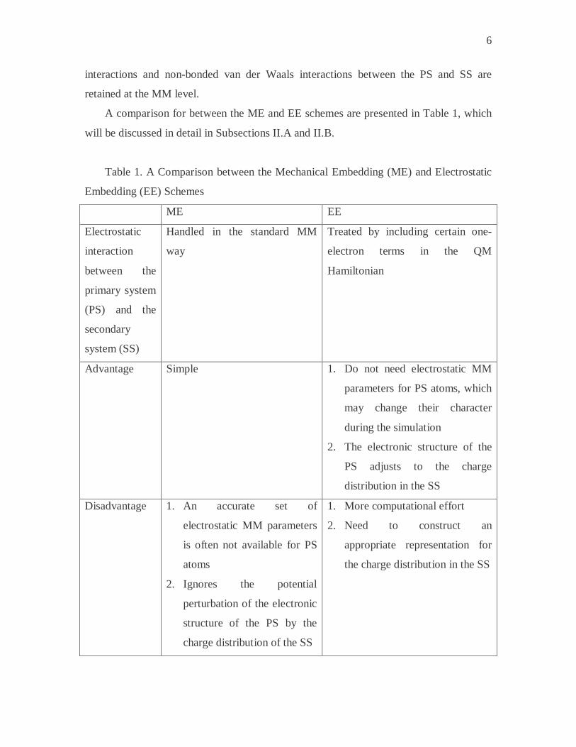
A comparison for between the ME and EE schemes are presented in Table 1, which

will be discussed in detail in Subsections II.A and II.B.

Table 1. A Comparison between the Mechanical Embedding (ME) and Electrostatic

Embedding (EE) Schemes

ME EE

Electrostatic

interaction

between the

primary system

(PS) and the

secondary

system (SS)

Handled in the standard MM

way

Treated by including certain one-

electron terms in the QM

Hamiltonian

Advantage Simple 1. Do not need electrostatic MM

parameters for PS atoms, which

may change their character

during the simulation

2. The electronic structure of the

PS adjusts to the charge

distribution in the SS

Disadvantage 1. An accurate set of

electrostatic MM parameters

is often not available for PS

atoms

2. Ignores the potential

perturbation of the electronic

structure of the PS by the

charge distribution of the SS

1. More computational effort

2. Need to construct an

appropriate representation for

the charge distribution in the SS

7

II.A. Mechanical Embedding?

The key difference between an ME scheme and an EE scheme is how they treat the

electrostatic interaction between PS and SS. An ME scheme handles the interaction at the

MM level, which is simpler. However, such a treatment has drawbacks. First, the

treatment requires an accurate set of MM parameters such as atom-centered point charges

for both the PS and SS. It is relatively easier to get such parameters for the SS, and the

problem with getting such parameters for the PS, where reactions are taking place, was

the central reason for moving from MM to QM in the first place. Since the charge

distribution in the PS usually changes as reaction progresses, the error in using a single

set of MM parameters could be very serious. The second drawback of an ME scheme is

that it ignores the potential perturbation of the electronic structure of the PS due to the

electrostatic interaction between the PS and SS. The atom-centered charges in the SS

polarize the PS and alter its charge distribution. This is especially a problem if the

reaction in the PS is accompanied by charge transfer. Another problematic situation

would be a system (e.g., an open-shell system containing transition metals) having

several electronic states close in energy, for which the polarization could change the

energetic order of these states, e.g., predicting a different ground state with a different

charge and/or spin distribution.

To deal with the lack of accurate MM electrostatic parameters for the PS atoms

during a reaction, one might consider obtaining these parameters dynamically as the

reaction progresses, e.g., deriving atom-centered point charges for the PS atoms when the

system evolutes along the reaction path. This idea works in principle, but in practice, it

requires a large PS to achieve the desired accuracy due to the second drawback of ME

schemes, which was just discussed above. That is, the PS system must be large enough to

assure that its calculated charge distribution is converged with respect to the location of

the QM/MM boundary. Moreover, an accurate and fast algorithm is necessary to derive

the MM electrostatic parameters on the fly (with no or only a little calibration by

experimental data or validation by doing pure MM simulation). These requirements will

apparently increase the computational effort considerably.

This problem motivates consideration of the mechanically embedded three-layer

ONIOM(MO:MO:MM) method.52 This method attempts to overcome the drawbacks of a

8

mechanically embedded two-layer ONIOM(MO:MM)39 by introducing a buffer (middle)

layer, which is treated by an appropriate lower-level QM theory (e.g., semi-empirical

molecular orbital theory), which is computationally less expensive than the method used

for the innermost primary subsystem. One can label such a treatment as QM1:QM2:MM

or QM1/QM2/MM. The second QM layer is designed to allow a consistent treatment of

the polarization of the active center by the environment. The new treatment does improve

the description, but, with mechanical embedding, it does not solve the problem

completely, since the QM calculation for the first layer is still performed in the absence

of the rest of the atoms.

II.B. Electrostatic Embedding?

In contrast to an ME scheme, an EE scheme does not require the MM electrostatic

parameters for the PS atoms, because the electrostatic interaction between PS and SS is

now treated at a more advanced level by including certain one-electron terms in the QM

Hamiltonian. The polarization of the PS by the charge distribution of the SS is also taken

into account automatically. The recent progress in the development of electrostatic

embedded ONIOM method137,138 reflects the trend of moving from ME to EE in QM/MM

methodology. The price to pay for this improvement is more complicated implementation

and increased computational cost.

The unsolved issue for EE schemes is how to construct the one-electron terms in the

effective QM Hamiltonian. As mentioned earlier, the simplest way is to represent the

charge distribution of the SS as a background of atom-centered partial charges. This is

further facilitated by the availability of a set of pre-parameterized MM point charges in

many MM force fields; these MM point charges have in principle been parameterized

consistently with the other MM parameters to give accurate MM energies, and they have

been validated by extensive test calculations. The use of these MM atom-centered partial

charges is very efficient, and it is the most popular way in constructing the effective QM

Hamiltonian. Nevertheless, the question is raised: are charge parameterized for a

particular MM context also appropriate for use in a QM Hamiltonian? In an extreme case,

for example, a zeolite-substrate system, the formal atomic charges used in aluminosilicate

force field are chosen to reproduce the structural rather than electrostatic data; such

9

charges may not be appropriate for the construction of the one-electron terms in the

effective QM Hamiltonian.56

The MM point charges actually include the contributions due to higher-order

multipoles implicitly, i.e., the higher-order contributions are folded into the zero-order

parameters. By considering higher-order multipole contributions explicitly, one might

increase the accuracy of calculated electrostatic interactions, but this makes the

implementation more difficult, and the computational costs grow. The development of

distributed multipole parameters is also a difficult and time-consuming task, but the

biggest obstacle is that the higher-order terms are generally sensitive to the geometry or

conformation changes.153-155 The high conformation-dependence of the multipole

expansion limits the transferability.156 For example, only about 20 amino acids are

commonly encountered in proteins. It would be ideal to have one set of parameters for

these 20 amino acids, which could be used to simulate any proteins, and it would be very

inconvenient if one had to develop a new set of parameters whenever another protein is

studied or whenever the conformation of a given protein changes considerably.

Another unsolved issue in ascertaining the best EE strategy is the question of the

polarization of the SS. In principle, the PS and SS will polarize each other until their

charge distributions are self-consistent; properly account for this in a computation is

usually accomplished by an iterative scheme157 (or matrix inversion) or by an extended

Lagrangian scheme.158 Ideally, an EE scheme should include this self-consistency; but

usually the charge distribution of the SS is considered frozen for a given set of SS nuclear

coordinates. Schemes that relax this constraint can be called self-consistent embedding

schemes (or polarized embedding schemes). However, self-consistency is difficult to

achieve, because it requires a polarizable MM force field,157-169 which has the flexibility

to respond to perturbation by an external electric field. Such flexibility is not available in

today’s most popular MM force fields, although research to develop a polarizable force

field has received much attention.164,166 Moreover, the use of a self-consistent embedding

scheme also brings additional complication to the treatment of the boundary between the

PS and SS, which we will discuss later in next section. Finally, it increases the

computational effort, since iterations are required to achieve self-consistent polarization

of the PS and SS. Thus, in most EE implementations, the PS is polarized by the SS, but

10

the SS is not polarized by the PS. Early examinations on the self-consistent embedding

scheme was carried out by Thompson and Schenter42 and Bakowies and Thiel.44 Their

treatments are based on models that describe the mutual polarization of QM and MM

fragments in the sprit of reaction field170-173 theory, with the difference that the response

is generated by a discrete reaction field (atomic polarizabilities) rather than a continuum.

Their results suggests that the polarization of the SS by the PS can be crucial in

applications involving a charged PS that generates large electric fields.

II.C. Interactions Other than Electrostatic

Although, as discussed above, the key difference between the ME and EE schemes

is the treatment of the electrostatic interaction between the PS and the SS, there are also

important issues involving in the treatments of the other interactions between the PS and

the SS. These interactions include the bonded (stretching, bending, and torsional)

interactions and the non-bonded van der Waals interactions, which are handled at the

MM level.

A similar question arises here, as in the case of electrostatic interactions for the ME

scheme, but now even for the EE schemes, i.e., all the interactions calculated at the MM

level rely on the availability of MM parameters for the PS atoms. These parameters are

not necessarily the same for the PS atoms in the reactant and product because the atom

types are changed for some atoms, e.g., a carbon atom may change from C=O type to

C−O−H type. Which set of MM parameters should we use? Should one switch between

two sets of MM parameters during a dynamics calculation following the reaction path?

Switching between these two sets of parameters during a dynamics calculation or along

the reaction path is not convenient, and, again, avoiding this was the one of the reasons

for moving up from MM to QM. Moreover, even if the switching between parameters

could be done, one does not know at which point along the reaction path it should be

done and how suddenly if the change is gradual. There is no unambiguous answer.

One key difference between the need for non-bonded electrostatic parameters and

the need for bonded parameters is that the latter requirement can always be obviated by

making the PS bigger, i.e., moving the QM-MM boundary out. The change of atom types

might change the force constants for associated bonded-interactions. Usually force

11

constants for stretches are much bigger than force constants for bends, and force

constants for torsions are the smallest. The changes of force constants due to the change

of atom types are often in this order, too. This provides us with gauge for monitoring the

error due to using a single set of MM parameters. The bonded interactions between PS

and SS are localized at the boundary. In principle, the use of a larger PS pushes the

boundary away from the reaction center and helps to alleviate the uncertainty due to

parameter choices, but at a price of increasing computational effort. In many cases,

though, enlarging the PS is not a practical solution. What then? Our suggestion is to keep

using one set of MM parameters, and examine whether the errors introduced by using one

set of parameters exceeds the errors produced by other approximations that are

introduced by the QM/MM framework. Although our treatment is not a perfect solution,

it is very practical, and it appears to be reasonable.

For the van der Waals interactions, any PS atoms that change atom types are

intrinsically ambiguous; this problem cannot be avoided even if a larger QM subsystem is

adopted. Fortunately, in practice, it does not appear to be a serious problem in most cases,

since the van der Waals interactions are significant only at short distances (as compared

to longer range forces associated charged species and permanent dipoles), and the use of

only one set of van der Waals parameters is often adequate.

II.D. Treating Solid-State Systems

So far we have been talking about QM/MM methodology in a very general sense. In

this subsection, we more specifically address some question about how to treat periodic

systems and other solid-state materials such as metals, metal oxides, and surface-

adsorbate systems. Excellent discussions47,56,74,85,96,97,101-103,108,115,133,140,145 are available

for many aspects, and we focus here especially on studies of zeolites.

As we mentioned above, the most important interaction between the PS and the SS

is the electrostatic interaction. Thus, the central problem in treating periodic systems like

the zeolite-substrate systems is how to incorporate the long-range electrostatic

interactions between the SS and PS into a cluster model. The basis idea174 is to develop a

representation of charge distribution with a finite number of multipoles (usually point

charges) to mimic the infinite and periodic charge distribution of the environment in

12

which the cluster model is embedded. This effective charge-distribution can be obtained

by minimizing the difference between the electrostatic potentials that are generated by the

effective charge distribution and by the original infinite and periodic charge distribution

at a set of sampling points at the active site. Additional effective core potentials can be

associated with selected point charges if needed. For example, parameterized effective

core potentials can be use to replace point charges that are close to anions in the PS in

order to reduce the overpolarization of these anions.175 By doing so, one truncates the

infinite and periodic system to a finite embedded cluster model, which is now much

easier to handle.

A simple example is the Surface Charge Representation of the Electrostatic

Embedding Potential (SCREEP) method, in which the electrostatic potential from the

infinite crystal lattice is modeled by a finite number (usually several hundred) of point

charges located on a surface enclosing the cluster.176 More sophisticated models97,101,103

also include polarization effects on the SS by using the shell-model.159 The shell model159

represents an ion, e.g., an O2– ion in silica, by a pair of charges, namely, a positive core

and a negative shell. The pair of charges are connected by a harmonic potential. The

positions of all charge are optimized to get the lowest energy, i.e., the polarization effect

is modeled as charge redistribution.

It is a concern that, in QM/MM calculations, as a consequence of the finite size of

the cluster, the calculated HOMO-LUMO gap for solid is still typically larger than that

for the corresponding extended solid, despite corrections to the energy to take into

account the electrostatic contribution of the MM region. One might expect this to cause

some errors in the calculation of absorption (of ions, electrons, or molecules) into the QM

center. One important question that seems to be involved is whether the neglect of orbital

interactions between the QM and MM subsystems underestimates the bandwidth of the

QM system. This would be a serious problem if the QM-MM boundary passed through a

conjugated system or a metallic region. But what if the boundary passes through a

covalent bond? First, it is important to keep in mind that the HOMO-LUMO gap is not a

physical observable, and the LUMO itself is somewhat arbitrary as long as it remains

unoccupied. (For example, the LUMO of Hartree-Fock theory is unphysical, and the

13

meaning of orbital energies in DFT is still a subject of debate.) It is most profitable to

cast the problem in terms of observables.

An example of a physical observable of concern would be the absorption energy of

an electron into the QM region, i.e., the electron affinity of a molecule in the QM region.

This is a difficult question to address because one of the main failings of QM/MM

methods is that they neglect charge transfer between the QM and MM subsystems,

although in reality there is almost always some charge transfer between non-identical

systems in close proximity, and it is not expected to an integer. Nevertheless we can

imagine the case of transferring an integer charge into the QM region and ask whether the

electron affinity might be systematically in error, due to a systematic error in the HOMO-

LUMO gap caused by neglecting the overlap of QM orbitals with the (missing) MM

orbitals. This would be hard to answer because the electron affinity of a subsystem is not

well defined. Therefore, one might ask a related practical question such as whether one

systematically underestimates the energy of anionic QM subsystems, such as

carboxylates. In practice, we have not seen such an effect. The errors due to the inexact

treatment of the electrostatic effects of the MM system are large enough that the error in

energies of reaction can be in either direction.

Another practical example might be the calculation of electronic excitation energies.

Is there a way, other than increasing the size of the QM region, to stabilize the excitation

energy? Or: can one calculate accurate electronic excitation energies of a non-isolated

QM system without converging the calculation with respect to enlarging the size of

subsystem that is treated quantum mechanically. We think that it is reasonable to hope

that one can do this, if one makes the QM/MM treatment sophisticated enough. For

example, one can obtain reasonable values for solvatochromic shifts from continuum

solvation models in which the solvent is not treated quantum mechanically.177

II.E. Adaptive QM/MM

An important issue that arises in simulating liquid-state phenomena and diffusion

through solids is the adaptive movement of the quantum mechanical region, which is

called the “hot spot”.50,77,116,178 Algorithms have been reported for liquid-phase

simulation that allow water molecules to enter and leave the QM region dynamically. The

14

basic idea is to identify a narrow “buffer-region” or “switching shell” between the QM

and MM regions. The cut-off is group-based, i.e., a solvent molecule like water is

considered to be in the buffer region when its center of mass is in the buffer region. In

order to avoid a discontinuity in the force as a solvent molecule enters or leaves the hot

spot, Rode and coworkers50 proposed to use a smooth function for the forces experienced

by the atoms in the buffer region to ensure a smooth transition between QM and MM

force. The smooth function takes the same form as the one179used in the CHARMM

program to handle the discontinuity in energy and force due to the use of cut-offs for non-

bonded (especially electrostatic) interactions. Despite its success, this treatment lacks a

unique definition for the energy, which is obtained by integration of the force. Later,

Kerdcharoen and Morokuma116 described another scheme to cope with the discontinuity.

In their scheme, two QM/MM calculations are performed for a given configuration of the

whole system. The first calculation is done with the atoms in the buffer region and the

atoms in the MM region treated at the MM level, and the second calculation is carried out

with the atoms in the buffer region and the atoms in the QM region treated at the QM

level. The total QM/MM energy is a weighted average of the QM/MM energies obtained

in these two calculations; the weight function is determined by the position of the atoms

in the buffer region. This treatment can be viewed as making a smooth connection of two

potential energy surfaces.

III. QM/MM Boundary Treatment

In this section, we examine the problem with a stronger microscope, and we consider

details, especially for the troublesome implementation of the EE scheme. In some cases,

the boundary between PS and SS does not go through a covalent bound, e.g., a molecule

being solvated in water, where the solute is the PS and the solvent (water) molecules is

the SS.36,69 The effective fragment potential method46 can also be considered as a special

case of MM in this catalog. In many cases, however, one cannot avoid passing the

boundary between the PS and SS through covalent bonds (e.g., in enzymes or reactive

polymers) or through ionic bonds (in solid-state catalysts). This is called cutting a bond.

In such cases, special care is required to treat the boundary, and this section (Section III)

is mainly concerned with this problem.

15

III.A. Link Atom or Local Orbital?

Treatments of the boundary between PS and SS regions can be largely grouped into

two classes. The first is the so-called link atom approach, where a link-atom is used to

saturate the dangling bond at the “frontier atom” of the PS. This link atom is usually

taken to be a hydrogen atom,34,39,52,72,106,116,119 or a parameterized atom, e.g., a one-free-

valence atom in the “connection atom”,70 “pseudobond”,82 and “quantum capping

potential”111 schemes, which involve a parameterized semi-empirical Hamiltonian70 or a

parameterized effective core potential (ECP)82,111 adjusted to mimic the properties of the

original bond being cut. The second class of QM/MM methods consists of methods that

use localized orbitals at the boundary between the PS and SS. An example is the so-called

local self-consistent field (LSCF) algorithm,35,38,43,51,112 where the bonds connecting the

PS and SS are represented by a set of strictly localized bond orbitals (SLBOs) that are

determined by calculations on small model compounds and assumed to be transferable.

The SLBOs are excluded from the self-consistent field (SCF) optimization of the large

molecule to prevent their admixture with other QM basis functions. Another approach in

the spirit of the LSCF method is the generalized hybrid orbital (GHO)

method.63,83,113,123,125,142,144,149 In this approach, a set of four sp3 hybrid orbitals is assigned

to each MM boundary atom. The hybridization scheme is determined by the local

geometry of the three MM atoms to which the boundary atom is bonded, and the

parametrization is assumed to be transferable. The hybrid orbital that is directed toward

the frontier QM atom is called the active orbital, and the other three hybrid orbitals are

called auxiliary orbitals. All four hybrid orbitals are included in the QM calculations, but

the active hybrid orbital participates in the SCF optimizations, while the auxiliary orbitals

do not.

Each kind of boundary treatment has its strength and weakness. The link atom

method is straightforward and is widely used. However, it introduces the artificial link

atoms that are not present in the original molecular system, and this makes the definition

of the QM/MM energy more complicated. It also presents complications in optimizations

of geometries. In addition, it is found, at least in the original versions of the link atom

method, that polarization of the bond between the QM frontier atom and the link atom is

unphysical due to the nearby point charge on the MM “boundary atom” (an MM

16

boundary atom is the atom whose bond to a frontier QM atom is cut). The distance

between the link atom and the MM boundary atom is about 0.5 Å in the case of cutting a

C−C bond (the bond distance is about 1.1 Å for a C-H bond and about 1.5 Å and for a C-

C bond). Similar problem is found in the case of cutting a Si−O bond (the bond distance

is about 1.4 Å for a Si−H bond and about 1.6 Å and for a Si−O bond). At such a short

distance, the validity of using a point charge to represent the distribution of electron

density is questionable. Special treatments are applied to the MM charges near the

boundary so as to avoid this unphysical polarization.33,44,70,71,82,93,110,124 We will discuss

this problem in more detail later Subsection III.B.

The methods using local orbitals are theoretically more fundamental than the

methods using link atoms, since they provide a quantum mechanical description of the

charge distribution around the QM/MM boundary. The delocalized representation of

charges in these orbitals helps to prevent or reduce the over-polarization that, as

mentioned above, is sometimes found in the link-atom methods. However, the local-

orbital methods are much more complicated than the link-atom methods. The local-

orbital method can be regarded as a mixture of molecular-orbital and valence-bond

calculations; a major issue in these studies is the implementation of orthogonality

constraints of MOs.142 Moreover, additional work is required to obtain an accurate

representation of the local orbitals before the actual start of a QM/MM calculation. For

example, in the LSCF method, the SLBOs are pre-determined by calculations on small

model compounds, and specific force field parameters are needed to be developed to

work with the SLBOs. In the GHO method, extensive parameterization for integral

scaling factors in the QM calculations is needed.63,125,142,144,149 Such parameters usually

require reconsideration if one switches MM scheme (e.g., from CHARMM to OPLS-

AA), QM scheme (e.g., from semi-empirical molecular orbital methods to density

functional theory or post-Hartree-Fock ab initio methods), or QM basis set. The low

transferability limits the wide application of the local orbital methods.

The performance of both the link-atom and local-orbital approaches has been

examined by extensive test calculations. The conclusion is that reasonably good accuracy

can be achieved by both approaches if they are used with special care. It is expected that

17

development and application of both the link-atom and local-orbital methods will

continue in the future.

III.B. Using Link-Atom Methods

A central objective in the development of a universal QM/MM algorithm is to make

the algorithm as general as possible and to avoid or to minimize the requirement of

introducing any new parameters. Thus, for example, one way to define a universally

applicable method would be that, when one makes an application to a new system, no

MM parameters need to be changed, no QM integral scaling factors needed to be

determined, no effective core potentials (ECP) needed to be developed. From this point

of view, the link-atom method seems very attractive. Furthermore the method will be

more easily built into a standard QM code if the link atom is an ordinary hydrogen atom

with a standard basis set. Methods having these features will be examined in more detail

in this section.

To facilitate our further discussion, we will label the atoms according to “tiers”. The

MM boundary atom will be denoted as M1. Those MM atoms directly bonded to M1 will

be called second-tier molecular mechanics atoms or M2; similarly, one defines M3 atoms

as those MM atoms bonded to M2 atoms … The QM boundary atom that is directly

connected to M1 is labeled Q1. Similarly, one defines Q2 and Q3 atoms in the QM

subsystem. We will denote the link-atom as HL, which stands for “hydrogen-link”,

emphasizing that an ordinary hydrogen atom is used/preferred.

18

III.B.1. Location of the Link-Atom

As we mentioned in the previous section, the link-atom method has its problems. The

first problem is the introduction of the coordinates of the link atom, which are extra

degrees of freedom. By definition, a link atom is neither a QM nor an MM atom, because

it is not present in the original PS or SS. This causes ambiguity to the definition of

QM/MM energy for the ES. One way to avoid this problem is to make the coordinates of

a link atom depend on the coordinates of the PS frontier atom and the SS boundary atom,

i.e., the Q1 and M1 atoms. Such a constraint removes the extra degrees of freedom due to

the link atom. Usually the link-atom is put on the line that connects the corresponding Q1

and M1 atoms. Morokuma and coworkers72,180 proposed to scaled the Q1−HL distance

R(Q1−HL) with respect to the Q1−M1 distance R(Q1−M1) by a scaling factor CHL:

R(Q1−HL) = CHL R(Q1−M1) (3)

During a QM/MM geometry optimization or a molecular dynamics of reaction path

calculation, the equilibrium Q1−HL and Q1−M1 distances are constrained to satisfy

equation (3). The scaling factor, CHL, depends on the nature of the bonds being cut and

constructed. It has been suggested72 that it should be the ratio of standard bond lengths

between Q1−HL and Q1−M1 bonds, which is close to 0.71 for replacement of a C−C

single bond by a C−H bond. This treatment is reasonable, and its simplicity facilitates

implementation of analytic energy derivatives (gradient and Hessians). However, the

meaning of “standard bond length” is ambiguous. Our treatment is to set the scaling

factor by

CHL = R0(Q1−H) / R0(Q1−M1), (4)

where R0(Q1−H) and R0(Q1−M1) are the MM bond distance parameters for the Q1−H

and Q1−M1 stretches in the employed MM force field, respectively.

It is worthwhile to mention that Eichinge et al.73 also proposed a scaled-bond-

distance scheme that is similar to the above scheme by Morokuma and coworkers.

However, the scheme by Eichinge et al. makes the scaling factor depend on the force

constants of the C−C stretch and C−H stretch instead of the bond distances, and it

introduces some additional terms to correct the energy.

19

III.B.2. MM Charges near the Boundary

Another problem (in fact, the problem that has caused the most concern) for the link

atom method, as we mention in the previous section, is the over-polarization of the

Q1−HL bond due to the nearby M1 point charge. The main reason for this problem is that

at such a short distance (usually about 0.5 Å in the case of cutting a C−C bond and about

0.2 Å in the case of cutting a Si−O bond), a point charge assigned to the M1 nucleus does

not provide a good approximation for the smeared distribution of charge density. For

nearby charge distributions, one must considers screening and charge penetration, and

dipole or higher order multipole moments can also become important. Various

approaches have been attempted to avoid or minimize this over-polarization effect, and

they are outlined below.

If a scheme does nothing to modify the MM charges, we label the scheme as straight-

electrostatic-embedding (SEE). The SEE scheme causes the over-polarization problem.

The simplest way to avoid over-polarization is to ignore the M1 charge by setting it to

zero;181 we call this method the Z1 scheme. One can also zero out both M1 and M2

charges; the method can be called Z2. If all M1, M2, and M3 charges are omitted,33 the

scheme is called Z3. The Z3 scheme is the default option for electrostatic embedding in

ONIOM calculations carried out by the Gaussian03 package;182 but Gaussian03 also

allows one to use scaling factors other than zero for M2, M3, and M4 charges (the M1

charge is always set to zero). The scaled-charge schemes are generalizations of the

eliminated-charge scheme. Schemes that eliminate or scale MM charges often result in

changing the net charge of the SS, e.g., a neutral SS might become partially charged, and

generate artifacts in the calculation of energies or spurious long-range forces.

In many force fields such as CHARMM, the neutrality of certain groups is enforced

during the parameterization by imposing a constraint that the sum of charges for several

neighboring atoms is zero. An improved eliminated-group-charge scheme58 takes

advantage of this feature by deleting the atomic charges for the whole group that contains

the M1 atom. This ensures that the net charge of the SS does not change. It has been

found that this scheme is more robust than the Z1, Z2, and Z3 schemes because it

preserves the charge for SS.

20

A shifted-charge scheme67 has been developed to work with force fields where the

neutral-groups feature is not available. (Of course, the scheme can also be used for force

fields having the neutral-groups feature). In this scheme, called the Shift scheme, the M1

charge is shifted evenly onto the M2 atoms that are connected to M1, and an additional

pair of point charges is placed in vicinity of the M2 atom in order to compensate for the

modification of the M1−M2 dipole by the initial shift.

As pointed out above, the over-polarization effect is largely due to the poor

approximation for the distribution of charge density around the M1 atom by a point

charge. Therefore, one might think of using a more realistic description for the charge

distribution. Recently, it has been proposed110,124 to use Gaussian charge distributions

instead of point charges for selected atoms.

Recently, we147

developed two new

schemes: a redistributed-

charge (RC) scheme and

a redistributed-charge-

and-dipole (RCD)

scheme, which are based

on combining the link-

atom treatment and the

local-orbital treatment.

As indicated in Fig. 2, both schemes use redistributed charges as molecular mechanical

mimics of the auxiliary orbitals associated with the MM boundary atom in the GHO

theory. In the RC scheme, the M1 charge is distributed evenly onto mid-points of the

M1−M2 bonds, i.e., at the nominal centers of the bond charge distributions. The

redistributed charge and M2 charges are further modified in the RCD scheme to restore

the original M1−M2 bond dipole. The RC and RCD schemes handle the charges in ways

that are justified as molecular mechanical analogs to the quantal description of the charge

distribution offered by GHO theory.

Fig. 2. The redistributed charge scheme (right) is a molecular

mechanical analog to the quantal description by the generalized hybrid

orbital (GHO) theory (left). The MM boundary atom and the active

hybrid orbital (shown in red) in the GHO theory are now modeled by an

H atom, and the auxiliary orbitals (shown in blue) are modeled by three

point charges.

21

IV. Validation of a QM/MM Algorithm

Validating QM/MM methods by comparing to high-level calculations or experiment

is essential, since the use of unvalidated methods is unacceptable. Although the

motivation for developing QM/MM methods is to apply them to large systems (e.g.,

reactions in the condensed phase, including liquids, enzymes, nanoparticles, and solid-

state materials), most of the validation studies have been based on small gas-phase model

systems, where a “model system” is a small- or medium-sized molecule. It is important,

in interpreting such validation tests, to keep two important issues in mind.

First, the molecular mechanics parameters, especially partial charges, are usually

designed for treating condensed-phase systems where partial charges are systematically

larger due to polarization effects in the presence of dielectric screening; thus electrostatic

effects of the MM subsystem may be overemphasized in the gas phase. Special attention

is given to alkyl groups that are frequently involved in these test examples, because a

non-polar C−C bond is often considered to be the most suitable place for putting the

QM/MM boundary. An alkyl group in the gas phase appears to be very unpolar, and the

C and H atoms are often assign atom-center point charges of small values. For example,

in a recent study,147 charges for the C and H atoms in a C2H6 molecule are –0.05 e and

0.02 e, respectively, as derived by the Merz-Singh-Kollmann33,183 electrostatic potential

(ESP) fitting procedure. An alkyl group becomes more polar in water or in other polar

solvents, and the point charges on the atoms in the alkyl group increase significantly. The

OPLS-AA force field assigns a charge of –0.18 e for each C atom and 0.06 e for each H

atom in the C2H6 molecule, and in the CHARMM force field, the values are even larger

(–0.27 e for each C atom and 0.09 e for each H atom). Our calculations147 on the proton

affinity of several gas-phase molecules having alkyl groups found much bigger errors

when using the charges developed for simulations in water than when using the ESP-

fitted charges. We believe that our conclusion is general since we tested several QM/MM

schemes that treat the MM charges near the boundary differently, and observed a similar

trend. We learned from this that it is very hard to test schemes designed for complex

processes in the condensed phase by carrying calculations on small molecules in the gas

phase.

22

It is probably more important to focus on the fact that the QM/MM interface can

introduce artifacts. Thus, the main goal of validation tests should usually be to ensure that

no unacceptably large energetic or structural artifacts are introduced, rather than to

achieve high quantitative accuracy for MM substituent effects. In this regard, a QM/MM

method is often tested by examples that are more difficult in one or another sense than

those in a normal application because one wants to know where the performance

envelope lies. Thus, calculations on examples having large proton affinities are very

suitable for testing. Proton or hydride transfer involves significant charge transfer and is

thus a crucial test for the treatment of electrostatic interactions (especially the procedure

for handling MM charges near the QM/MM boundary) in a QM/MM method. A large

value of the energy difference between the reactant and product also helps us to draw

conclusions that are not compromised by the intrinsic uncertainty of the QM/MM

approach.

The proton affinity of CF3CH2O−, where CF3 is the SS and CH2O− is the PS, is one

of these difficult examples, due to both the close location of the reaction center to the

boundary and the presence of significant point charges on the atoms in the CF3 group

near the boundary. A recent study147 on this difficult example by making comparisons

between full QM computations and various QM/MM schemes with the ESP-fitted MM

charges for the CF3 group. The QM/MM schemes include the capped PS, the SEE

scheme, three eliminated-charge (Z1, Z2, and Z3) schemes, the Shift scheme, the RC

scheme, and the RCD scheme. It is found that the Shift and RCD schemes, both of which

preserve both the charge of the SS and the M1−M2 bond dipoles, are superior to the other

schemes in comparison. For example, when, the errors for the RC and Shift schemes are

1 and 2 kcal/mol, respectively. It is also found that the largest error is caused by the Z1

scheme (75 kcal/mol), where neither the charge nor the dipole is preserved. The results

suggest that it is critical to retain the feature of charge distribution near the QM/MM

boundary. By this criterion, the SEE scheme does not seem to be too bad with an error of

9 kcal/mol; actually it is even better than the RC scheme (error of 12 kcal/mol) and the

best charge-elimination schemes Z2 and Z3 (errors of 25 kcal/mol). However, the error in

the optimized Q1−M1 (C−C) distance is 3 to 4 times larger for the SEE scheme than for

23

any of the other schemes to which comparison was made, and this makes the SEE scheme

a poor choice in practical applications.

V. Implementation and Software

As summarized in a recent review article, there are basically three kinds of

programming architecture for implementing QM/MM methods.

1. Extension of a “traditional” QM package by incorporating the MM environment

as a perturbation. Many QM packages are have added or are adding the QM/MM

options. A well-known example is the ONIOM method implemented in

Gaussian03 (http://www.gaussian.com/). Other examples include the ADF

(http://www.scm.com/), CHIMISTE/MM (http://www.lctn.uhp-

nancy.fr/logiciels.html), GAMES-UK (http://www.cse.clrc.ac.uk/qcg/gamess-uk/),

MCQUB (http://www.chem.umn.edu/groups/gao/software.htm), MOLCAS

(http://www.teokem.lu.se/molcas/), MOZYME

(http://www.chem.ac.ru/Chemistry/Soft/MOZYME.en.html), and QSite

(http://www.schrodinger.com/Products/qsite.html) packages.

2. Extension of a “traditional” MM package by incorporating a QM code as a force-

field extension. Examples include AMBER (http://amber.scripps.edu/), CHARMM

(http://www.charmm.org/), and CGPLUS (http://comp.chem.umn.edu/cgplus/).

3. A central control program interfacing QM and MM packages, where users can

select between several QM and/or MM packages. For example, CHEMSHELL

(http://www.cse.clrc.ac.uk/qcg/chemshell/) and QMMM

(http://comp.chem.umn.edu/qmmm/) belong to this catalog.

Each kind of program architecture has its own merits and disadvantages. The options

based on extension of traditional QM and/or MM packages can make use of the many

features of the original program, for example, the ability of the MM program to

manipulate large, complex biological systems. The disadvantage is that both options need

modification of the codes.

The third option is based on module construction and is more flexible. It often needs

no or little modification on the original QM and MM programs. The program is

automatically updated when the QM or MM packages that it interfaces are updated. The

24

drawback is that it requires a considerable amount of effort to transfer the data between

the QM and MM packages, which is usually done by reading data from files, rearranging

the data, and writing the data to files. Such additional manipulations can lower the

efficiency.

Our recently developed program QMMM adopts the third programming architecture.

The QMMM program currently interfaces Gaussian03 for doing QM computations and

TINKER for doing MM calculations. Geometry optimization and transition-state searching

can be done by using the algorithm built into the QMMM program or by using an

optimizer in the Gaussian03 program via the external option of Gaussian03. In addition

to the RC and RCD schemes, the QMMM program also implements several other schemes

such as the SEE, scaled-charge, and shifted-charge schemes for handling the MM point

charges near the QM/MM boundary. Currently we are working on combination of the

QMMM program with the molecular dynamics program POLYRATE

(http://comp.chem.umn.edu/polyrate/) for doing QM/MM direct dynamics calculations.184

VI. What do We Learn from a QM/MM Calculation?

As discussed in the introduction, one benefit that QM/MM calculations bring to us is

the inclusion of the effect of a chemical environment (secondary subsystem, SS) on the

reaction center (primary subsystem, PS). The interactions between a PS and an SS are of

two kinds: (1) interactions that are significant even at long range (electrostatic

interaction), and (2) interactions that are local (bonded interactions) or are only

significant at short range (van der Waals interactions). The electrostatic interactions are

usually dominant, as they perturb the electronic structure of the PS, and they often have

great effects on energetic quantities such as the reaction energy. The bonded and van der

Waals interaction act in other ways; for example in enzyme reactions or solid-state

reactions, they impose geometry constraints by providing a rigid frame in the active site

or lattice site to hold the PS. (In fact, the electrostatic interaction will also affect the

equilibrium geometry of the PS.)

A practical way to examine the effect of the environment is to compare quantities

such as reaction energies or barrier heights as calculated from an isolated QM model and

from a QM/MM model. Usually such quantities show significant differences for

25

processes that involve significant changes in the charge distribution. The calculations for

proton transfer reactions are good examples (see the discussion on the proton affinity in

Section IV).

However, one sometimes finds the same or very similar reaction energies and barrier

heights from isolated QM model systems and QM/MM model calculations. This is likely

to be observed for a reaction without much change transfer, e.g., a radical abstraction

reaction. This does not mean that the SS does not affect the PS. In such a case, it is likely

that the effect due to the SS is roughly the same for the reactant, transition state, and

product, and the cancellation leads to small net effects. An approximate analysis of the

effects due to SS can be obtained by an energy-decomposition as follows (see also Fig.

3).

The energy difference between the QM energy for

the PS (or CPS, i.e., a PS capped by link atoms) in the

gas phase and the QM energy for the PS in an

interacting MM environment is defined by

EPS/MM = E(QM;PS**) − E(QM;PS), (5)

where E(QM;PS**) is the QM energy for the PS

embedded in the background point charges of SS, and

E(QM;PS) is the QM energy for the PS in the gas

phase. In either case, the geometry is fully optimized at

the corresponding level of theory, i.e., at the QM/MM

level for E(QM;PS**) and at the QM level for

E(QM;PS). Equation (5) provides a measure of the

magnitude of the perturbation on the QM subsystem

due to the MM subsystem. Generally speaking, the two geometries in Equation (5) are

different. We further decompose EPS/MM into two contributions: the energy due to the

polarization of the background point charges (Epol) and the energy due to the geometry

distortion from the PS in the gas phase (Esteric), which are defined as

Epol = E(QM;PS**) − E(QM;PSdis), (6)

Esteric = E(QM;PSdis) − E(QM;PS), (7)

Figure 3. Decomposition of energy

due to MM environment into two

contributions: the energy due to the

polarization by the background point

charges (Epol) and the energy due to

the geometry distortion (Esteric). See

Equations (5) to (8).

26

EPS/MM = Epol + Esteric, (8)

where E(QM;PSdis) is the gas-phase single-point PS energy for the QM/MM optimized

geometry, i.e., one takes the PS geometry that resulted from QM/MM optimization and

removes the MM point charges. Although such an energy-decomposition is approximate,

it is informative and provides us deeper understanding of the QM/MM calculations.

The energy decomposition is applied to a reaction that we studied recently147 (Fig. 4).

CH3 + CH3CH2CH2OH CH4 + CH2CH2CH2OH (R-1)

The PS is CH3 + CH3CH2, giving rise to a CPS as CH3 + CH3CH3. The SS is CH2OH.

For each of the reactant, saddle point, and product of this reaction, we found a small

steric effect (0.1 kcal/mol) and a dominant polarization effect (9 kcal/mol). It is not

surprising to see such a small setic effect, since the distortion of geometry for the CPS

from the fully relaxed geometry in the gas phase can be rather small. The critical point is

that the energies due to geometry distortion and polarization are so similar along the

reaction path that they almost cancel out, giving rise to negligibly small net contributions

to the reaction energy and barrier height.

27

Although the MM

environment does not have a

large net effect on the relative

energies of the H atom transfer

reaction (R1), it does have

effects on the electronic

structure of the CPS through

polarization and perturbs the

charge distribution. The ESP-

fitted charges in Fig. 4 clearly

show a trend of stepwise

change from the unperturbed

CPS (denoted as CPS), to the

CPS with distorted geometry

(CPSdis), then to the CPS

embedded in the background

point charge distribution (CPS**), and finally to the ES, as modeled by full QM

calculations. It is interesting to note that the Cb−Cc bond seems to be very unpolar

according to the CPS calculations, with a small bond dipole pointing from the Cb to the

Cc atom. The CPS** calculations predict that the Cb−Cc bond is more polar, with a

larger and inverse bond dipole pointing from the Cc to the Cb atom, in qualitative

agreement with full QM calculations. The CPS** result is generally closer to the full QM

results, suggesting that QM/MM calculations provide a more realistic description for the

QM subsystem than the isolated gas-phase QM model calculations.

The conclusion that for a reaction that does not involve much charge transfer, the

inclusion of the electrostatic field of the SS will yield small effects in relative energies

but large affects in the electronic structure of the PS also gain supports from studies of

zeolite-substrate systems.56 In Ref. 56, it has been found that the inclusion of the

electrostatic field of the SS slightly alters the barrier (by ca. 2 kcal/mol) of a methyl shift

reaction over a zeolite acid site, but has considerably large effects on the charge

Fig. 4. ESP-fitted charges for selected atoms in reaction CH3 +

CH3CH2CH2OH CH4 + CH2CH2CH2OH.

28

distribution and vibrational frequencies. For example, the charge on the O atoms is

changed by 0.16 e.

Comparing the results of QM/MM calculations with experimental results is the

ultimate test of a QM/MM scheme. However, such a comparison is not trivial, and we

mention here several points that need attention in general.

First, one should consider what kinds of experimental results, including their

temperature and pressure, are most informative to be compared, and how reliable these

results are, i.e., what is the error bar associated with the observed quantity. It is also

important to understand, in the case of the experimental data were derived from fitting to

a simplified model, what kinds of assumptions and simplifications have been invoked. In

addition, it is important to understand the parameters characterizing the QM/MM

calculations. For example, are the results converged with respect to increasing the size of

the PS, increasing the QM level of theory and/or basis sets, tightening of the optimization

convergence threshold, and increasing the cutoff distance or cutoff threshold if any, in the

calculation of MM nonbonded interactions? If we are treating a complex system like an

enzyme solvated in water, is the phase space sampled adequately? If we cannot afford an

extensive phase-space sampling, can we examine several representative conformations?

Do we need to consider potential anharmonicity in vibrational analysis?

Of particular importance is to separate, at least approximately, the errors due to the

insufficient QM treatment of the PS and the errors due to the insufficient consideration of

the SS effect. As we showed previously, the barrier height and reaction energy are often

not sensitive to the electrostatic interaction between the PS and SS for a reaction that

does not involve significant charge transfer. In such a case, it may be more desirable to

increase the QM level of theory to improve the results than to improve the MM level or

the QM/MM interface. On the other hand, for reactions that are sensitive to the

electrostatic interaction between the PS and the SS, simply increasing the QM level of

theory does not necessarily improve the reliability.

29

V. Where Do We Go from Here?

Combining QM and MM by applying them to separate subsystems with a boundary in

physical space is very natural, and it is safe to say that it is now a permanent part of the

theoretical toolbox. However, there are other ways to combine QM and MM, and future

work may see greater use of methods that blend QM and MM more intimately.

A venerable example of such an approach is the use of quantum mechanics to suggest

new functional forms for molecular mechanics. The oldest example would be the Morse

curve, which was originally derived by a QM treatment of H2+.185 Replacing a harmonic

bond stretching potential by a Morse curve allows MM to treat bond breaking. It is much

harder to treat synchronous bond breaking and bond forming, but this was also

accomplished in the early days of quantum mechanics, resulting in the London

equation.186-188 Raff189 was apparently the first to combine the valence-bond-derived QM

London equation with molecular mechanics terms to make a QM/MM reactive potential,

and in recent years many other workers,190,191 especially Espinosa-Garcia and

coworkers,192-197have made fruitful use of this technique. Various workers, of whom we

single out Brenner198-200 and Goddard and coworkers201-204 for noteworthy systematic

efforts, have made generalizations to more complex reactive systems. However, these

methods are neither universal nor systematically improvable like the methods discussed

in Sections III and IV.

One way to make the combination of valence bond theory and molecular mechanics

more universal and systematic is multi-configuration molecular mechanics205-209

(MCMM). MCMM combines QM and MM in a different way than QM/MM; in MCMM

the whole system is treated by QM, and simultaneously the whole system is treated by

MM. In fact, every atom is treated by two different MM schemes, one corresponding to a

reactant and the other to a product, and the two MM energy expansions interact by a

2 × 2 configuration interaction matrix highly reminiscent of London’s 2 × 2 matrix

matrices or the similar 2 × 2 matrices used by Raff,189 Warshel and Weiss,210 and others.

However, in MCMM the off-diagonal elements of the Hamiltonian are not empirical MM

parameters as in previous work, but rather are determined by systematically improvable

QM methods. The method is very young but very promising.

30

In the future, we can expect further progress in MCMM. One straightforward

improvement is to use QM/MM to replace QM in determination of the off-diagonal

element of the Hamiltonian matrices, and this scheme can be called QM/MM-based-

MCMM, or QM/MM-MCMM for short. Another even more promising scheme is to

combine MCMM with MM in the “same way” that QM is combined with MM in

combined QM/MM methods. That is, use MCMM to replace the QM in QM/MM; this

scheme can be called MCMM-based-QM/MM, or MCMM-QM/MM. Both schemes

make MCMM suitable for handling very large systems. Work in this direction is in

progress, and encouraging preliminary results have been obtained.211

Another area of future improvement is use of improved MM formalisms in QM/MM

methods. We have already mentioned polarizable MM force fields (see Section II.B).166

Even without allowing polarization, the charges in MM force fields can be improved in

various ways. In particular, various charge models have been developed or are in

refinement. Examples include the restrained electrostatic potential212 (RESP) fitting

procedure and its latest improved version “dynamically generated restrained electrostatic

potential” (DRESP)213 for QM/MM calculations, the family of CMx (x = 1,214 2,215,216,

3217-219, and 4220) charge models, the charge equilibration221,222 (CEq) method, and the

consistent charge equilibration (CQEq)223-225 method.

An interesting and important future development is the adaptive QM/MM scheme,

which was discussed in Section II E. If we allow atoms to be exchanged between the QM

and MM regions, can we take one more step forward, allowing fractional (or whole)

charges to be transferred between the QM and MM regions? Of course, to accomplish

this goal, we need to work out how to describe the electronic structure of a system with

fractional electrons.226,227

Another important trend we can expect to see in the near future is the incorporation in

MM of methods for modeling metallic systems that were developed in the physics

community. For example, just as simplified valence bond theory can be used to obtain

functional forms for extending MM to reacting systems, the second-moment

approximation to the tight-binding approximation (also known as extended Hückel

theory) can be used to obtain new forms for modeling metals.228 An example of this kind

31

of approach is the use of the embedded-atom functional form to develop MM potentials

for Al nanoparticles.229

A theme that emerges from several of the approaches discussed in this section is the

difficulty of classifying the potential energy function as QM or MM. For example, is the

embedded-atom method an approximate version of density functional theory or is it MM?

Is MCMM an automatic fitting method for QM energies or is it an extension of MM to

reactive systems? We prefer to think of these methods as new kinds of QM-MM hybrids

where the QM-MM combination is more intimate than in the first generation of combined

QM/MM methods.

32

Acknowledgments

This work is supported in part by the National Science Foundation and the Office of

Naval Research. The authors are grateful to Jiali Gao and Jingzhi Pu for valuable

discussions.

References (1) van Gunsteren, W. F.; Berendsen, H. J. C.; Geurtsen, R. G.; Zwinderman, H. R. J. Ann. NY Acad. Sci. 1986, 482, 287. (2) Allinger, N. L.; Yuh, Y. H.; Lii, J. H. J. Am. Chem. Soc. 1989, 111, 8551. (3) Lii, J. H.; Allinger, N. L. J. Am. Chem. Soc. 1989, 111, 8566. (4) Lii, J. H.; Allinger, N. L. J. Am. Chem. Soc. 1989, 111, 8576. (5) Mayo, S. L.; Olafson, B. D.; Goddard, W. A., III. J. Phys. Chem. 1990, 94, 8897. (6) Rappé, A. K.; Casewit, C. J.; Colwell, K. S.; Goddard III, W. A.; Skid, W. M. J. Am. Chem. Soc. 1992, 114, 10024. (7) Casewit, C. J.; Colwell, K. S.; Rappé, A. K. J. Am. Chem. Soc. 1992, 114, 10035. (8) Casewit, C. J.; Colwell, K. S.; Rappé, A. K. J. Am. Chem. Soc. 1992, 114, 10046. (9) Rappé, A. K.; Colwell, K. S.; Casewit, C. J. Inorg. Chem. 1993, 32, 3438. (10) Cornell, W. D.; Cieplak, P.; Bayly, C. I.; Gould, I. R.; Merz, K. M., Jr.; Ferguson, D. M.; Spellmeyer, D. C.; Fox, T.; Caldwell, J. W.; Kollman, P. A. J. Am. Chem. Soc. 1995, 117, 5179. (11) Pearlman, D. A.; Case, D. A.; Caldwell, J. W.; Ross, W. S.; Cheatham, T. E. I.; DeBolt, S.; Ferguson, D.; Seibel, G.; Kollman, P. A. Computer Physics Communications 1995, 91, 1. (12) Halgren, T. A. J. Comput. Chem. 1996, 17, 490. (13) Halgren, T. A. J. Comput. Chem. 1996, 17, 520. (14) Halgren, T. A. J. Comput. Chem. 1996, 17, 552. (15) Halgren, T. A.; Nachbar, R. B. J. Comput. Chem. 1996, 17, 587. (16) Halgren, T. A. J. Comput. Chem. 1996, 17, 616. (17) Jorgensen, W. L.; Maxwell, D. S.; Tirado-Rives, J. J. Am. Chem. Soc. 1996, 118, 11225. (18) MacKerell, A. D., Jr.; Bashford, D.; Bellott, M.; Dunbrack, R. L.; Evanseck, J. D.; Field, M. J.; Fischer, S.; Gao, J.; Guo, H.; Ha, S.; Joseph-McCarthy, D.; Kuchnir, L.; Kuczera, K.; Lau, F. T. K.; Mattos, C.; Michnick, S.; Ngo, T.; Nguyen, D. T.; Prodhom, B.; Reiher, W. E., III; Roux, B.; Schlenkrich, M.; Smith, J. C.; Stote, R.; Straub, J.; Watanabe, M.; Wiorkiewicz-Kuczera, J.; Yin, D.; Karplus, M. J. Phys. Chem. B 1998, 102, 3586. (19) Jorgensen, W. L.; McDonald, N. A. Theochem 1998, 424, 145. (20) McDonald, N. A.; Jorgensen, W. L. J. Phys. Chem. B 1998, 102, 8049.

33

(21) Ewig, C. S.; Thacher, T. S.; Hagler, A. T. J. Phys. Chem. B 1999, 103, 6999. (22) Rizzo, R. C.; Jorgensen, W. L. J. Am. Chem. Soc. 1999, 121, 4827. (23) Allinger, N. L.; Durkin, K. A. J. Comput. Chem. 2000, 21, 1229. (24) Kaminski, G. A.; Friesner, R. A.; Tirado-Rives, J.; Jorgensen, W. L. J. Phys. Chem. B 2001, 105, 6474. (25) Price, M. L. P.; Ostrovsky, D.; Jorgensen, W. L. J. Comput. Chem. 2001, 22, 1340. (26) Hill, J.-R.; Sauer, J. J. Phys. Chem. 1994, 98, 1238. (27) Hill, J.-R.; Sauer, J. J. Phys. Chem. 1995, 99, 9536. (28) Schröder, K.-P.; Sauer, J. J. Phys. Chem. 1996, 100, 11043. (29) Sierka, M.; Sauer, J. Faraday Discuss. 1997, 106, 41. (30) Landis, C. R.; Cleveland, T.; Firman, T. K. J. Am. Chem. Soc. 1998, 120, 2641. (31) Firman, T. K.; Landis, C. R. J. Am. Chem. Soc. 2001, 123, 11728. (32) Warshel, A.; Levitt, M. Journal of molecular biology 1976, 103, 227. (33) Singh, U. C.; Kollmann, P. A. J. Comput. Chem. 1986, 7, 718. (34) Field, M. J.; Bash, P. A.; Karplus, M. J. Comput. Chem. 1990, 11, 700. (35) Ferenczy, G. G.; Rivail, J.-L.; Surjan, P. R.; Naray-Szabo, G. J. Comput. Chem. 1992, 13, 830. (36) Gao, J.; Xia, X. Science (Washington, DC, United States) 1992, 258, 631. (37) Åaqvist, J.; Warshel, A. Chem. Rev. 1993, 93, 2523. (38) Thery, V.; Rinaldi, D.; Rivail, J.-L.; Maigret, B.; Ferenczy, G. G. J. Comput. Chem. 1994, 15, 269. (39) Maseras, F.; Morokuma, K. J. Comput. Chem. 1995, 16, 1170. (40) Stanton, R. V.; Hartsough, D. S.; Merz, K. M., Jr. J. Comput. Chem. 1995, 16, 113. (41) Thompson, M. A. J. Phys. Chem. 1995, 99, 4794. (42) Thompson, M. A.; Schenter, G. K. J. Phys. Chem. 1995, 99, 6374. (43) Assfeld, X.; Rivail, J.-L. Chem. Phys. Lett. 1996, 263, 100. (44) Bakowies, D.; Thiel, W. J. Phys. Chem. 1996, 100, 10580. (45) Bakowies, D.; Thiel, W. J. Comput. Chem. 1996, 17, 87. (46) Day, P. N.; Jensen, J. H.; Gordon, M. S.; Webb, S. P.; Stevens, W. J.; Krauss, M.; Garmer, D.; Basch, H.; Cohen, D. J. Chem. Phys. 1996, 105, 1968. (47) Eichler, U.; Kölmel, C. M.; Sauer, J. J. Comput. Chem. 1996, 18, 463. (48) Eurenius, K. P.; Chatfield, D. C.; Brooks, B. R.; Hodoscek, M. Int. J. Quantum. Chem. 1996, 60, 1189. (49) Gao, J. Rev. Comput. Chem. 1996, 7, 119. (50) Kerdcharoen, T.; Liedl, K. R.; Rode, B. M. Chem. Phys. 1996, 211, 313. (51) Monard, G.; Loos, M.; Thery, V.; Baka, K.; Rivail, J.-L. Int. J. Quantum. Chem. 1996, 58, 153. (52) Svensson, M.; Humbel, S.; Froese, R. D. J.; Matsubara, T.; Sieber, S.; Morokuma, K. J. Phys. Chem. 1996, 100, 19357. (53) Bersuker, I. B.; Leong, M. K.; Boggs, J. E.; Pearlman, R. S. Int. J. Quantum. Chem. 1997, 63, 1051. (54) Cummins, P. L.; Gready, J. E. J. Comput. Chem. 1997, 18, 1496.

34

(55) Gao, J.; Alhambra, C. J. Chem. Phys. 1997, 107, 1212. (56) Sherwood, P.; De Vries, A. H.; Collins, S. J.; Greatbanks, S. P.; Burton, N. A.; Vincent, M. A.; Hillier, I. H. Faraday Discus. 1997, 106, 79. (57) Tongraar, A.; Liedl, K. R.; Rode, B. M. J. Phys. Chem. A 1997, 101, 6299. (58) Antes, I.; Thiel, W. ACS Symposium Series 1998, 712, 50. (59) Bentzien, J.; Florian, J.; Glennon, T. M.; Warshel, A. ACS Symposium Series 1998, 712, 16. (60) Bersuker, I. B.; Leong, M. K.; Boggs, J. E.; Pearlman, R. S. ACS Symposium Series 1998, 712, 66. (61) Burton, N. A.; Harrison, M. J.; Hart, J. C.; Hillier, I. H.; Sheppard, D. W. Faraday Discuss. 1998, 110, 463. (62) Froese, R. D. J.; Musaev, D. G.; Morokuma, K. J. Am. Chem. Soc. 1998, 120, 1581. (63) Gao, J.; Amara, P.; Alhambra, C.; Field, M. J. J. Phys. Chem. A 1998, 102, 4714. (64) Kaminski, G. A.; Jorgensen, W. L. J. Phys. Chem. B 1998, 102, 1787. (65) Merz, K. M., Jr. ACS Symposium Series 1998, 712, 2. (66) Mordasini, T.; Thiel, W. Chimia 1998, 52, 288. (67) Sinclair, P. E.; de Vries, A.; Sherwood, P.; Catlow, C. R. A.; van Santen, R. A. J. Chem. Soc. Faraday Trans. 1998, 94, 3401. (68) Stefanovich, E. V.; Truong, T. N. ACS Symposium Series 1998, 712, 92. (69) Woo, T. K.; Cavallo, L.; Ziegler, T. Theor. Chem. Acc. 1998, 100, 307. (70) Antes, I.; Thiel, W. J. Phys. Chem. A 1999, 103, 9290. (71) de Vries, A. H.; Sherwood, P.; Collins, S. J.; Rigby, A. M.; Rigutto, M.; Kramer, G. J. J. Phys. Chem. B 1999, 103, 6133. (72) Dapprich, S.; Komiromi, I.; Byun, K. S.; Morokuma, K.; Frisch, M. J. THEOCHEM 1999, 461-462, 1. (73) Eichinger, M.; Tavan, P.; Hutter, J.; Parrinello, M. J. Chem. Phys. 1999, 110, 10452. (74) Hillier, I. H. THEOCHEM 1999, 463, 45. (75) Monard, G.; Merz, K. M., Jr. Acc. Chem. Res. 1999, 32, 904. (76) Lyne, P. D.; Hodoscek, M.; Karplus, M. J. Phys. Chem. A 1999, 103, 3462. (77) Marini, G. W.; Liedl, K. R.; Rode, B. M. J. Phys. Chem. A 1999, 103, 11387. (78) Philipp, D. M.; Friesner, R. A. J. Comput. Chem. 1999, 20, 1468. (79) Pitarch, J.; Pascual-Ahuir, J. L.; Silla, E.; Tunon, I.; Ruiz-Lopez, M. F. J. Comput. Chem. 1999, 20, 1401. (80) Turner, A. J.; Moliner, V.; Williams, I. H. Phys. Chem. Chem. Phys. 1999, 1, 1323. (81) Woo, T. K.; Margl, P. M.; Deng, L.; Cavallo, L.; Ziegler, T. ACS Symposium Series 1999, 721, 173. (82) Zhang, Y.; Lee, T.-S.; Yang, W. J. Chem. Phys. 1999, 110, 46. (83) Amara, P.; Field, M. J.; Alhambra, C.; Gao, J. Theor. Chem. Acc. 2000, 104, 336. (84) Byun, K.; Gao, J. J. Mol. Graphics Model. 2000, 18, 50.

35

(85) Derenzo, S. E.; Klintenberg, M. K.; Weber, M. J. J. Chem. Phys. 2000, 112, 2074. (86) Field, M. J.; Albe, M.; Bret, C.; Martin, F. P.-D.; Thomas, A. J. Comput. Chem. 2000, 21, 1088. (87) Gogonea, V.; Westerhoff, L. M.; Merz, K. M., Jr. J. Chem. Phys. 2000, 113, 5604. (88) Hall, R. J.; Hindle, S. A.; Burton, N. A.; Hillier, I. H. J. Comput. Chem. 2000, 21, 1433. (89) Kairys, V.; Jensen, J. H. J. Phys. Chem. A 2000, 104, 6656. (90) Moliner, V.; Williams, I. H. Chem. Commun. 2000, 1843. (91) Murphy, R. B.; Philipp, D. M.; Friesner, R. A. J. Comput. Chem. 2000, 21, 1442. (92) Murphy, R. B.; Philipp, D. M.; Friesner, R. A. Chem. Phys. Lett. 2000, 321, 113. (93) Reuter, N.; Dejaegere, A.; Maigret, B.; Karplus, M. J. Phys. Chem. A 2000, 104, 1720. (94) Röthlisberger, U.; Carloni, P.; Doclo, K.; Parrinello, M. J. Biol. Inorg. Chem. 2000, 5, 236. (95) Sherwood, P. In Modern Methods and Algorithms of Quantum Chemistry; Grotendorst, J., Ed.; NIC-Directors: Princeton, 2000; Vol. 3; pp 285. (96) Sierka, M.; Sauer, J. J. Chem. Phys. 2000, 112, 6983. (97) Sushko, P. V.; Shluger, A. L.; Catlow, C. R. A. Surface Science 2000, 450, 153. (98) Vreven, T.; Morokuma, K. J. Comput. Chem. 2000, 21, 1419. (99) Woo, T. K.; Blöchl, P. E.; Ziegler, T. Theochem 2000, 506, 313. (100) Cui, Q.; Elstner, M.; Kaxiras, E.; Frauenheim, T.; Karplus, M. J. Phys. Chem. B 2001, 105, 569. (101) French, S. A.; Sokol, A. A.; Bromley, S. T.; Catlow, C. R. A.; Rogers, S. C.; King, F.; Sherwood, P. Angew. Chem. 2001, 113, 4569. (102) Khaliullin, R. Z.; Bell, A. T.; Kazansky, V. B. J. Phys. Chem. A 2001, 105, 10454. (103) Nasluzov, V. A.; Rivanenkov, V. V.; Gordienko, A. B.; Neyman, K. M.; Birkenheuer, U.; Rösch, N. J. Chem. Phys. 2001, 115, 8157. (104) Nicoll, R. M.; Hindle, S. A.; MacKenzie, G.; Hillier, I. H.; Burton, N. A. Theor. Chem. Acc. 2001, 106, 105. (105) Poteau, R.; Ortega, I.; Alary, F.; Solis, A. R.; Barthelat, J. C.; Daudey, J. P. J. Phys. Chem. A 2001, 105, 198. (106) Vreven, T.; Mennucci, B.; da Silva, C. O.; Morokuma, K.; Tomasi, J. J. Chem. Phys. 2001, 115, 62. (107) Worthington, S. E.; Krauss, M. J. Phys. Chem. B 2001, 105, 7096. (108) Batista, E. R.; Friesner, R. A. J. Phys. Chem. B 2002, 106, 8136. (109) Colombo, M. C.; Guidoni, L.; Laio, A.; Magistrato, A.; Maurer, P.; Piana, S.; Rohrig, U.; Spiegel, K.; Sulpizi, M.; VandeVondele, J.; Zumstein, M.; Röthlisberger, U. Chimia 2002, 56, 13. (110) Das, D.; Eurenius, K. P.; Billings, E. M.; Sherwood, P.; Chatfield, D. C.; Hodoscek, M.; Brooks, B. R. J. Chem. Phys. 2002, 117, 10534.

36

(111) DiLabio, G. A.; Hurley, M. M.; Christiansen, P. A. J. Chem. Phys. 2002, 116, 9578. (112) Ferré, Nicolas; Assfeld, X.; Rivail, J.-L. J. Comput. Chem. 2002, 23, 610. (113) Gao, J.; Truhlar, D. G. Annu. Rev. Phys. Chem. 2002, 53, 467. (114) Gogonea, V. Internet Electronic J. Mol. Design 2002, 1, 173. (115) Hermida-Ramón, J. M.; Karlström, G.; Lindh, R. J. Phys. Chem. B 2002, 106, 7115. (116) Kerdcharoen, T.; Morokuma, K. Chem. Phys. Lett. 2002, 355, 257. (117) Laio, A.; VandeVondele, J.; Röthlisberger, U. J. Chem. Phys. 2002, 116, 6941. (118) Lennartz, C.; Schaefer, A.; Terstegen, F.; Thiel, W. J. Phys. Chem. B 2002, 106, 1758. (119) Morokuma, K. Phil. Trans. Roy. Soc. London, Ser. A 2002, 360, 1149. (120) Rajamani, R.; Gao, J. J. Comput. Chem. 2002, 23, 96. (121) Schöneboom, J. C.; Lin, H.; Reuter, N.; Thiel, W.; Cohen, S.; Ogliaro, F.; Shaik, S. J. Am. Chem. Soc. 2002, 124, 8142. (122) Titmuss, S. J.; Cummins, P. L.; Rendell, A. P.; Bliznyuk, A. A.; Gready, J. E. J. Comput. Chem. 2002, 23, 1314. (123) Truhlar, D. G.; Gao, J.; Alhambra, C.; Garcia-Viloca, M.; Corchado, J.; Sanchez, M. L.; Villa, J. Acc. Chem. Res. 2002, 35, 341. (124) Amara, P.; Field, M. J. Theor. Chem. Acc. 2003, 109, 43. (125) Devi-Kesavan, L. S.; Garcia-Viloca, M.; Gao, J. Theor. Chem. Acc. 2003, 109, 133. (126) Dinner, A. R.; Lopez, X.; Karplus, M. Theor. Chem. Acc. 2003, 109, 118. (127) Hu, H.; Elstner, M.; Hermans, J. Proteins 2003, 50, 451. (128) Kongsted, J.; Osted, A.; Mikkelsen, K. V.; Christiansen, O. J. Phys. Chem. A 2003, 107, 2578. (129) Li, G.; Zhang, X.; Cui, Q. J. Phys. Chem. B 2003, 107, 8643. (130) Loferer, M. J.; Loeffler, H. H.; Liedl, K. R. J. Comput. Chem. 2003, 24, 1240. (131) Molina, P. A.; Sikorski, R. S.; Jensen, J. H. Theor. Chem. Acc. 2003, 109, 100. (132) Mordasini, T.; Curioni, A.; Andreoni, W. J. Biol. Chem. 2003, 278, 4381. (133) Sherwood, P.; de Vries, A. H.; Guest, M. F.; Schreckenbach, G.; Catlow, C. R. A.; French, S. A.; Sokol, A. A.; Bromley, S. T.; Thiel, W.; Turner, A. J.; Billeter, S.; Terstegen, F.; Thiel, S.; Kendrick, J.; Rogers, S. C.; Casci, J.; Watson, M.; King, F.; Karlsen, E.; Sjovoll, M.; Fahmi, A.; Schafer, A.; Lennartz, C. Theochem 2003, 632, 1. (134) Sulpizi, M.; Laio, A.; VandeVondele, J.; Cattaneo, A.; Röthlisberger, U.; Carloni, P. Proteins 2003, 52, 212. (135) Swart, M. Int. J. Quantum. Chem. 2003, 91, 177. (136) Tresadern, G.; Faulder, P. F.; Gleeson, M. P.; Tai, Z.; MacKenzie, G.; Burton, N. A.; Hillier, I. H. Theor. Chem. Acc. 2003, 109, 108. (137) Vreven, T.; Morokuma, K.; Farkas, O.; Schlegel, H. B.; Frisch, M. J. J. Comput. Chem. 2003, 24, 760. (138) Vreven, T.; Morokuma, K. Theor. Chem. Acc. 2003, 109, 125. (139) Yang, W.; Drueckhammer, D. G. J. Phys. Chem. B 2003, 107, 5986.

37

(140) Herschend, B.; Baudin, M.; Hermansson, K. J. Chem. Phys. 2004, 120, 4939. (141) Laio, A.; Gervasio, F. L.; VandeVondele, J.; Sulpizi, M.; Röthlisberger, U. J. Phys. Chem. B 2004, 108, 7963. (142) Pu, J.; Gao, J.; Truhlar, D. G. J. Phys. Chem. A 2004, 108, 632. (143) Riccardi, D.; Li, G. H.; Cui, Q. J. Phys. Chem. B 2004, 108, 6467. (144) Pu, J.; Gao, J.; Truhlar, D. G. J. Phys. Chem. A 2004, 108, 5454. (145) Bludsky, O.; Silhan, M.; Nachtigall, P. J. Phys. Chem. B 2005, asap. (146) Gregersen, B. A.; York, D. M. J. Phys. Chem. B 2005, 109, 536. (147) Lin, H.; Truhlar, D. G. J. Phys. Chem. A 2005, 109, 3991. (148) Nam, K.; Gao, J.; York, D. M. J. Chem. Theory Comput. 2005, 1, 2. (149) Pu, J.; Truhlar, D. G. ChemPhysChem 2005, in press. (150) Wanko, M.; Hoffmann, M.; Strodel, P.; Koslowski, A.; Thiel, W.; Neese, F.; Frauenheim, T.; Elstner, M. J. Phys. Chem. B 2005, 109, 3606. (151) Zhang, Y. J. Chem. Phys. 2005, 122, 024114. (152) Chemical Applications of Atomic and Molecular Electrostatic Potentials. Reactivity, Structure, Scattering, and Energetics of Organic, Inorganic, and Biological Systems; Politzer, P.; Truhlar, D. G., Eds.; Plenum: New York, 1981. (153) Price, S. L.; Stone, A. J. J. Chem. Soc. Faraday Trans.1992, 88, 1755. (154) Koch, U.; Popelier, P. L. A.; Stone, A. J. Chem. Phys. Lett. 1995, 238, 253. (155) Matta, C. F.; Bader, R. F. W. Proteins: Struct. Func. Genet. 2000, 40, 310. (156) Minikis, R. M.; Kairys, V.; Jensen, J. H. J. Phys. Chem. A 2001, 105, 3829. (157) Stillinger, F. H.; David, C. W. J. Chem. Phys. 1978, 69, 1473. (158) Sprik, M.; Klein, M. L. J. Chem. Phys. 1988, 89, 7556. (159) Dick Jr., B. G.; Overhauser, A. W. Phy. Rev. 1958, 112, 90. (160) Van Belle, D.; Prevost, M.; Lippens, G.; Wodak, S. J. ACS Symposium Series 1994, 568, 318. (161) Kowall, T.; Foglia, F.; Helm, L.; Merbach, A. E. J. Am. Chem. Soc. 1995, 117, 3790. (162) Banks, J. L.; Kaminski, G. A.; Zhou, R.; Mainz, D. T.; Berne, B. J.; Friesner, R. A. J. Chem. Phys. 1999, 110, 741. (163) Martinez, J. M.; Hernandez-Cobos, J.; Saint-Martin, H.; Pappalardo, R. R.; Ortega-Blake, I.; Marcos, E. S. J. Chem. Phys. 2000, 112, 2339. (164) Rick, S. W.; Stuart, S. J. Rev. Comput. Chem. 2002, 18, 89. (165) Lamoureux, G.; MacKerell, A. D.; Roux, B. J. Chem. Phys. 2003, 119, 5185. (166) Ponder, J. W.; Case, D. A. Adv. Protein Chem. 2003, 66, 27. (167) Ren, P.; Ponder, J. W. J. Phys. Chem. B 2003, 107, 5933. (168) Kaminski, G. A.; Stern, H. A.; Berne, B. J.; Friesner, R. A. J. Phys. Chem. A 2004, 108, 621. (169) Patel, S.; Mackerell, A. D., Jr.; Brooks, C. L., III. J. Comput. Chem. 2004, 25, 1504. (170) Rinaldi, D.; Rivail, J. L. Theor. Chim. Acta 1973, 32, 57.

38

(171) Storer, J. W.; Giesen, D. J.; Hawkins, G. D.; Lynch, G. C.; Cramer, C. J.; Truhlar, D. G.; Liotard, D. A. ACS Symposium Series 1994, 568, 24. (172) Tomasi, J. ACS Symposium Series 1994, 1994, 10. (173) Cramer, C. J.; Truhlar Donald, G. Continuum solvation models. In Solvents Effects and Chemical Reactivity; Tapia, O., Bertran, J., Eds.; Kluwer: Dordrecht, 1996; pp 1. (174) Bacalis, N. C.; Kunz, A. B. Phys. Rev. B 1985, 32, 4857. (175) Pascual, J.; Pettersson, L. G. M. Chem. Phys. Lett. 1997, 270, 351. (176) Stefanovich, E. V.; Truong, T. N. J. Phys. Chem. B 1998, 102, 3018. (177) Li, J.; Cramer, C. J.; Truhlar, D. G. Int. J. Quantum Chem. 2000, 77, 264. (178) Yagüe, J. I.; Mohammed, A. M.; Loeffler, H.; Rode, B. M. J. Phys. Chem. A 2001, 105, 7646. (179) Brooks, B. R.; Bruccoleri, R. E.; Olafson, B. D.; States, D. J.; Swaminathan, S.; Karplus, M. J. Comput. Chem. 1983, 4, 187. (180) Humbel, S.; Sieber, S.; Morokuma, K. J. Chem. Phys. 1996, 105, 1959. (181) Waszkowycz, B.; Hillier, I. H.; Gensmantel, N.; Payling, D. W. J. Chem. Soc. Perkin Trans. 2 1991, 2025. (182) Frisch, M. J.; Trucks, G. W.; Schlegel, H. B.; Scuseria, G. E.; Robb, M. A.; Cheeseman, J. R.; Montgomery, J., J. A.; Vreven, T.; Kudin, K. N.; Burant, J. C.; Millam, J. M.; Iyengar, S. S.; Tomasi, J.; Barone, V.; Mennucci, B.; Cossi, M.; Scalmani, G.; Rega, N.; Petersson, G. A.; Nakatsuji, H.; Hada, M.; Ehara, M.; Toyota, K.; Fukuda, R.; Hasegawa, J.; Ishida, M.; Nakajima, T.; Honda, Y.; Kitao, O.; Nakai, H.; Klene, M.; Li, X.; Knox, J. E.; Hratchian, H. P.; Cross, J. B.; Adamo, C.; Jaramillo, J.; Gomperts, R.; Stratmann, R. E.; Yazyev, O.; Austin, A. J.; Cammi, R.; Pomelli, C.; Ochterski, J. W.; Ayala, P. Y.; Morokuma, K.; Voth, G. A.; Salvador, P.; Dannenberg, J. J.; Zakrzewski, V. G.; Dapprich, S.; Daniels, A. D.; Strain, M. C.; Farkas, O.; Malick, D. K.; Rabuck, A. D.; Raghavachari, K.; Foresman, J. B.; Ortiz, J. V.; Cui, Q.; Baboul, A. G.; Clifford, S.; Cioslowski, J.; Stefanov, B. B.; Liu, G.; Liashenko, A.; Piskorz, P.; Komaromi, I.; Martin, R. L.; Fox, D. J.; Keith, T.; Al-Laham, M. A.; Peng, C. Y.; Nanayakkara, A.; Challacombe, M.; Gill, P. M. W.; Johnson, B.; Chen, W.; Wong, M. W.; Gonzalez, C.; A., P. J. Gaussian03; Gaussian, Inc.: Pittsburgh PA, 2003. (183) Besler, B. H.; Jr., K. M. M.; Kollman, P. A. J. Comput. Chem. 1990, 11, 431. (184) Truhlar, D. G.; Gordon, M. S. Science 1990, 249, 491. (185) Morse, P. M. Phy. Rev. 1929, 34, 57. (186) London, F. Z. Elektrochem. 1929, 35, 552. (187) Eyring, H.; Polanyi, M. Z. Phys. Chem. B 1931, 12, 279. (188) Parr, C. A.; Truhlar, D. G. J. Phys. Chem. 1971, 75, 1844. (189) Raff, L. M. J. Chem. Phys. 1974, 60, 2220. (190) Steckler, R.; Dykema, K. J.; Brown, F. B.; Hancock, G. C.; Truhlar, D. G.; Valencich, T. J. Chem. Phys. 1987, 87, 7024. (191) Jordan, M. J. T.; Gilbert, R. G. J. Chem. Phys. 1995, 102, 5669. (192) Espinosa-García, J.; Corchado, J. C. J. Chem. Phys. 1996, 105, 3517. (193) Espinosa-García, J.; Corchado, J. C. J. Chem. Phys. 2000, 112, 5731. (194) Espinosa-Garcia, J.; Rangel, C.; Navarrete, M.; Corchado, J. C. J. Chem. Phys. 2004, 121, 5098.

39

(195) Navarrete, M.; Rangel, C.; Espinosa-Garcia, J.; Corchado, J. C. J. Chem. Theory Comput. 2005, 1, 337. (196) Rangel, C.; Espinosa-Garcia, J. J. Chem. Phys. 2005, 122, 134315. (197) Rangel, C.; Navarrete, M.; Espinosa-Garcia, J. J. Phys. Chem. A 2005, 109, 1441. (198) Brenner, D. W. Phys. Rev. B 1990, 42, 9458. (199) Brenner, D. W. Phys. Stat. Sol. (b) 2000, 217, 23. (200) Brenner, D. W.; Shenderova, O. A.; Harrison, J. A.; Stuart, S. J.; Ni, B.; Sinnott, S. B. J. Phys.: Condens. Matter 2002, 14, 782. (201) Duin, A. C. T. v.; Dasgupta, S.; Lorant, F.; Goddard, W. A. J. Phys. Chem. A 2001, 105, 9396. (202) Goddard, W. A., III ; Zhang, Q.; Uludogan, M.; Strachan, A.; Cagin, T. In Fundamental Physics of Ferroelectrics 2002; Cohen, R. E., Ed.; American Institute of Physcis: Pasadena, 2002; Vol. 626; pp 45. (203) Duin, A. C. T. v.; Strachan, A.; Stewman, S.; Zhang, Q.; Xu, X.; Goddard, W. A. J. Phys. Chem. A 2003, 107, 3803. (204) Cheung, S.; Deng, W.-Q.; van Duin, A. C. T.; Goddard, W. A. J. Phys. Chem. A 2005, 109, 851. (205) Kim, Y.; Corchado, J. C.; Villa, J.; Xing, J.; Truhlar, D. G. J. Chem. Phys. 2000, 112, 2718. (206) Albu, T. V.; Corchado, J. C.; Truhlar, D. G. J. Phys. Chem. A 2001, 105, 8465. (207) Truhlar, D. G. J. Phys. Chem. A 2002, 106, 5048. (208) Lin, H.; Pu, J. Z.; Albu, T. V.; Truhlar, D. G. J. Phys. Chem. A 2004, 108, 4112. (209) Kim, K. H.; Kim, Y. J. Chem. Phys. 2004, 120, 623. (210) Warshel, A.; Weiss, R. M. J. Am. Chem. Soc. 1980, 102, 6218. (211) Lin, H.; Truhlar, D. G., to be published. (212) Bayly, C. I.; Cieplak, P.; Cornell, W. D.; Kollman, P. A. J. Phys. Chem. 1993, 97, 10269. (213) Laio, A.; VandeVondele, J.; Rothlisberger, U. J. Phys. Chem. B 2002, 106. (214) Storer, J. W.; Giesen, D. J.; Cramer, C. J.; Truhlar, D. G. J. Comput.-Aid. Mol. Des. 1995, 9, 87. (215) Li, J.; Zhu, T.; Cramer, C. J.; Truhlar, D. G. J. Phys. Chem. A 1998, 102, 1820. (216) Li, J.; Williams, B.; Cramer, C. J.; Truhlar, D. G. J. Chem. Phys. 1999, 110, 724. (217) Winget, P.; Thompson, J. D.; Xidos, J. D.; Cramer, C. J.; Truhlar, D. G. J. Phys. Chem. A 2002, 106, 10707. (218) Brom, J. M.; Schmitz, B. J.; Thompson, J. D.; Cramer, C. J.; Truhlar, D. G. J. Phys. Chem. A 2003, 107, 6483. (219) Thompson, J. D.; Cramer, C. J.; Truhlar, D. G. J. Comput. Chem. 2003, 24, 1291. (220) Kelly, C.; Cramer, C. J.; Truhlar Donald, G., to be published. (221) Mortier, W. J.; Ghosh, S. K.; Shankar, S. J. Am. Chem. Soc. 1986, 108, 4315.

40

(222) Rappé, A. K.; Goddard, W. A. J. Phys. Chem. 1991, 95, 3358. (223) Kitao, O.; Ogawa, T. Mol. Phys. 2003, 101, 3. (224) Ogawa, T.; Kurita, N.; Sekino, H.; Kitao, O.; Tanaka, S. Chem. Phys. Lett. 2003, 374, 271. (225) Ogawa, T.; Kurita, N.; Sekino, H.; Kitao, O.; Tanaka, S. Chem. Phys. Lett. 2004, 397, 382. (226) Gogonea, V.; Merz, K. M., Jr. J. Phys. Chem. B 2000, 104, 2117. (227) Tavernelli, I.; Vuilleumier, R.; Sprik, M. Phys. Rev. Lett. 2002, 88, 213002. (228) Ackland, G. J.; Finnis, M. W.; Vitek, V. J. Phys. F: Met. Phys. 1988, 18, L153. (229) Jasper, A. W.; Schultz, N. E.; Truhlar, D. G. J. Phys. Chem. B 2005, 109, 3915.