Geological Survey of New South Wales

Quarterly NotesSeptember 2015 No 145

© State of New South Wales through Department of Industry, Skills and Regional Development 2015.

Papers in Quarterly Notes are subject to external review. External reviewers for this issue were David Higgins (Geological Survey of Victoria) and Olivier Rey-Lescure (University of Newcastle). Their assistance is appreciated.

Quarterly Notes is published to give wide circulation to results of studies in the Geological Survey of New South Wales. Papers are also welcome that arise from team studies with external researchers. Contact: simone.meakin@industry.nsw.gov.auISSN 0155-3410 (print)ISSN 2204-4329 (online)

AUTHORSGlen Phillips1, Gary G. Colquhoun1,

Kyle S. Hughes1 and Liann Deyssing2

Geological Survey of New South Wales1516 High Street, Maitland, NSW 2320

2161 Kite Street, Orange, NSW 2800

Seamless geology of New South Wales: approach, methodology and application

AbstractThe Geological Survey of New South Wales (GSNSW) Seamless Geology Database is a compilation of the state’s best available geological mapping data in an internally consistent format. This report documents the public release of the geodatabase, which at present consists of a dynamic geological model of the eastern area of NSW covered by UTM Zone 56. The geodatabase structure allocates geological data into individual layers that represent key stages in the geological evolution of the state. For UTM Zone 56, data is assigned to one of the following layers: (i) Basement — New England and Lachlan orogens; (ii) Permian–Triassic Basins — Sydney, Gunnedah and Bowen basins; (iii) Great Australian Basin — Clarence–Moreton, Ipswich and Surat basins; (iv) Mesozoic igneous province; (v) Cenozoic sedimentary province; and (vi) Cenozoic igneous province. The approach taken to build the geological model for UTM Zone 56 involved merging disparate datasets deemed the best-available mapping data for particular regions. Initial problems encountered during the compilation and merging stages include: significant georeferencing errors inherited from older maps compiled on poor base-map data; spatial and stratigraphic mismatches across map joins, where linework did not connect or rock units were called different things across the map boundary; and mapping data that was acquired at markedly different scales (1:25 000 to 1:250 000), resulting in a variable degree of data resolution. To seamlessly merge these datasets, the following workflow was used: (i) convert all existing data into a consistent statewide format; (ii) rectify georeferencing problems; (iii) edge-match geological contacts across dataset boundaries; and (iv) re-code rock units using the new statewide stratigraphic naming convention. Using this approach, a new dynamic geological model of UTM Zone 56 was constructed. The geodatabase is also linked with the GSNSW Geoscientific Data Warehouse (GDW), which contains information on the character of rock units. Consequently, the Seamless Geodatabase can act as a spatial search engine that accesses geological data stored in the GDW.

Keywords: seamless geology, Geographic Information Systems, geodatabase

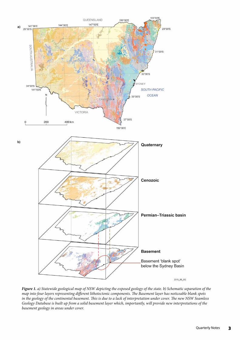
IntroductionThe advent of Geographic Information Systems (GIS) has changed the way geological data is managed. Traditionally, the Geological Survey of New South Wales (GSNSW) produced hard copy map sheets that show the distribution of exposed lithological units and geological features. While such maps are excellent tools for visualising geological data, their application beyond this is limited. Firstly, hard copy maps pose significant space restrictions which limit the amount of information that can be displayed. This restricts the amount of attribution data (which describes the characteristics of a particular rock unit) that can be shown on a map sheet. Consequently, information concerning the rock type, age and composition has to be simplified to physically fit on the map sheet. Alternatively, maps with a lot of attribution data have large swathes of text that dominate the sheet, which in turn limits the scale at which the map can be displayed. Secondly, hard copy maps produced by the GSNSW have historically been produced at a regional scale (1:250 000), which limits the resolution at which spatial data can be shown. Given the space restrictions posed by the hard copy map format, the published scale of these map sheets is commonly far removed from the best resolution of the available mapping data.

GIS provides an ideal platform to organise, view and interrogate geological data. Firstly, data can be organised in a layered format, in turn allowing geological data to be arranged in a comparable format to that observed in nature. That is, data pertaining to basement or basin geology can be organised into a series of overlapping layers that can be analysed separately, or overlaid and compared. Notably, this data structure replicates the organisation of geological units in nature, both in time and space. Secondly, space limitations associated with printed maps can be overcome in the digital environment. Attribution data such as age, composition, structural kinematics or grade of metamorphism can be attached to a lithological unit or a structural feature in the geodatabase, which can be accessed through a spatial query of the geodatabase. This removes the disconnect between spatial and attribute data that characterises printed maps. Thirdly, GIS geodatabases allow the user to display and interrogate the data at a variety of scales. Importantly, high resolution data pertaining to very detailed mapping can be integrated with low resolution data associated with broad scale regional mapping. As a result, low and high resolution data can be merged and displayed, which has always been problematic given the regional scales required for the display of statewide maps (Figure 1a).

2 September 2015

Contents

Abstract 1

Introduction 2

A historical perspective 4

The NSW Seamless Geology Database 5

UTM Zone 56 seamless geology 7

Data sources 7

Approach and methodology 10

Applications 16

Conclusion 19

Acknowledgements 19

References 19

Mobile seamless geology 20

Appendix: Data sources for the UTM Zone 56 23

Technical editing: Simone Meakin

Production co-ordination Simone Meakin and general editing : and Geneve Cox

Geospatial information: Kate Holdsworth

Layout: Nicole Edwards

DisclaimerThe information (and links) contained in this publication is based on knowledge and understanding at the time of writing (July, 2015). However, because of advances in knowledge, users are reminded of the need to ensure that the information upon which they rely is up to date and to check the currency of the information with the appropriate officer of the Department of Industry, Skills and Regional Development 2015 or the user’s independent adviser. The product trade names in this publication are supplied on the understanding that no preference between equivalent products is intended and that the inclusion of a product name does not imply endorsement by the department over any equivalent product from another manufacturer.

Copyright© State of New South Wales through Department of Industry, Skills and Regional Development 2015 You may copy, distribute and otherwise freely deal with this publication for any purpose, provided that you attribute the Department of Trade and Investment, Regional Infrastructure and Services as the owner.

Cover image: Inset map from the seamless geodatabase of the northern Sydney Basin (green) and southern Tamworth Belt (grey and blue). 1cm = approx. 4 km.

3Quarterly Notes

Figure 1. a) Statewide geological map of NSW depicting the exposed geology of the state. b) Schematic separation of the map into four layers representing different lithotectonic components. The Basement layer has noticeable blank spots in the geology of the continental basement. This is due to a lack of interpretation under cover. The new NSW Seamless Geology Database is built up from a solid basement layer which, importantly, will provide new interpretations of the basement geology in areas under cover.

4 September 2015

A historical perspectiveThe need for a database to host the GSNSW digital data was first recognised in the late 1990s. By that time, the GSNSW had hundreds of vector geology datasets ranging from detailed mapping at 1:25 000 to regional statewide datasets at 1:2 500 000. Digital data at the time was largely used for individual projects and therefore lacked a consistent structure and common format, which created difficulties in reconciling datasets from different projects. A further prompt for the development of a new geodatabase framework was the phasing out of Esri® GIS data formats, such as ArcInfo coverages and ArcView shapefiles, which were heavily used by the GSNSW. These factors led to a re-think about the way the GSNSW edited, stored and archived vector geology data, along with our approach to geological map production. Consequently, the NSW Statewide Geology Geodatabase Project was initiated with the aim of developing a new methodology for acquiring and managing digital geological map data that is consistent at a statewide level.

Early attempts at developing such a model were offered to a committee of Australian government geoscience agencies — Government Geoscience Information Policy Advisory Committee (GGIPAC) now known as the Government Geoscience Information Committee (GGIC) — as the basis for an Australian national geological map model. In 2003, a working party developed a conceptual model for the agencies to use. This model subsequently fed into the early stages of the GeoSciML Project, an international project which aims to create a standard model for serving geological map data over the web (www.geosciml.org). The GSNSW developed a conceptual model and deployed it as an Esri geodatabase. This model is believed to be the first geological mapping geodatabase in the world to be fully implemented by a government agency and was made available on the Esri website for download. Over the next 18 months, all GSNSW 1:250 000 scale geological mapping datasets were moved into the new Statewide Geology Geodatabase schema.

By the beginning of 2009, the NSW Statewide Geology Geodatabase was in urgent need of an upgrade, so was remodelled and upgraded. The restructure of the geodatabase was undertaken with digital field and office data capture in mind, and to improve compatibility with emerging geoscience data standards. The new geodatabase structure was introduced in late 2009, with a detailed workflow document for capturing geological data. This approach is now used in all GSNSW geological mapping and compilation projects. In addition to the development of the new geodatabase schema, the existing digital

The vision of the GSNSW Statewide Seamless Geology Project (SSGP) is to compile the best available geological data of the state into an internally consistent geodatabase. Historically, data acquired by the GSNSW has been restricted to regional mapping projects, which has resulted in the creation of regional datasets that are somewhat irreconcilable at a statewide level. A primary aim of the project is to merge these datasets into a single dynamic statewide geological model that can be interrogated at the best resolution available. To do this, the datasets have to be merged to remove evidence of pre-existing joins between the datasets, along with employing a consistent stratigraphic naming convention. A further goal of the project is to improve the basement maps. In the past, mapping has also focussed on documenting the exposed geology (Figure 1a), with little attempt made to extrapolate rock units or geological features under cover. This approach resulted in large swathes of the basement being uncharacterised (Figure 1b). A major outcome of the SSGP is the development of a solid basement layer that merges mapped and interpreted geology. By integrating map data with new geological interpretations based on geophysical data, solid lithological and structural interpretations of the basement are now available. This solid geology layer is a powerful tool that allows stakeholders to ‘peek’ under cover and to assess the nature of rock units or structures. In the past, these undercover areas have remained as basement ‘blank spots’ on the maps, thus rendering them potentially underutilised (Figure 1b).

This report outlines the history of the project and the methodology used to construct the geological model for Universal Transverse Mercator (UTM) Zone 56. The database can be downloaded in ArcGIS and MapInfo formats at http://www.resourcesandenergy.nsw.gov.au/miners-and-explorers/geoscience-information/products-and-data/geoscience-data-resources/geoscience-data-packages/data/seamless-geology-data-package-zone-56. As well as explaining the methodology used to construct the NSW Seamless Geology Database, we present some applications of the new geodatabase, including how it can be used to access geological data. To cover these topics, this report comprises four parts, namely: (i) a historical perspective to the GSNSW Statewide Seamless Geology Project; (ii) an introduction to the new geodatabase; (iii) the methodology used to construct the geological model for UTM Zone 56; and (iv) some applications of the new geodatabase. Furthermore, we also provide details of our new Mobile Maps platform (http://dwh.minerals.nsw.gov.au/CI/warehouse/view/mobileapps), which allows map viewing and interrogation on Android and Apple smartphones and tablets. In time, all seamless geodatabases released by the GSNSW will be available in both GIS and Mobile Map formats.

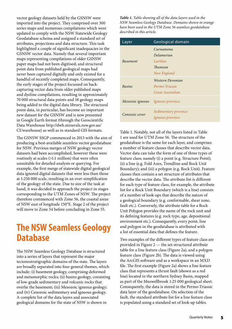
Table 1. Notably, not all of the layers listed in Table 1 are used for UTM Zone 56. The structure of the geodatabase is the same for each layer, and comprises a number of feature classes that describe vector data. Vector data can take the form of one of three types of feature class; namely (i) a point (e.g. Structure Point); (ii) a line (e.g. Fold Axes, Trendline and Rock Unit Boundary); and (iii) a polygon (e.g. Rock Unit). Feature classes then contain a set structure of attributes that describe the vector data. The attribute list is different for each type of feature class, for example, the attribute list for a Rock Unit Boundary (which is a line) consists of a number of look-ups that describe the nature of a geological boundary (e.g. conformable, shear zone, fault etc.). Conversely, the attribute table for a Rock Unit Polygon provides the name of the rock unit and its defining features (e.g. rock type, age, depositional environment etc.). Consequently, every point, line and polygon in the geodatabase is attributed with a list of essential data that defines the feature.

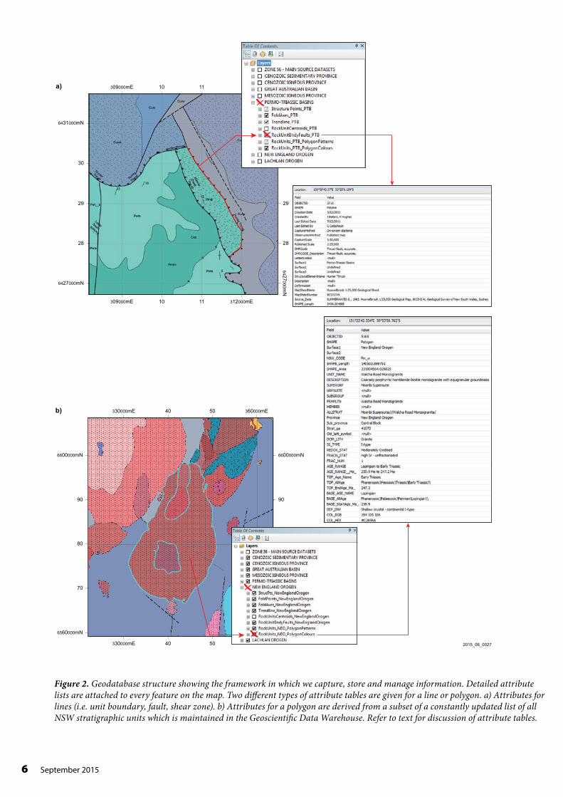
Two examples of the different types of feature class are provided in Figure 2 — the set-structured attribute table for a line feature class (Figure 2a), and a polygon feature class (Figure 2b). The data is viewed using the ArcGIS software and as a workspace in an MXD file. The first example (Figure 2a) shows a line feature class that represents a thrust fault (shown as a red line) located in the northern Sydney Basin, mapped as part of the Muswellbrook 1:25 000 geological sheet. Consequently, the data is stored in the Permo-Triassic data layer of the geodatabase. On selection of the fault, the standard attribute list for a line feature class is populated using a standard set of look-up tables.

vector geology datasets held by the GSNSW were imported into the project. They comprised over 300 series maps and numerous compilations which were updated to comply with the NSW Statewide Geology Geodatabase schema and assigned a standard set of attributes, projections and data structure. This task highlighted a couple of significant inadequacies in the GSNSW vector data. Namely that several important maps representing compilations of older GSNSW paper maps had not been digitised; and structural point data from published geological maps had never been captured digitally and only existed for a handful of recently completed maps. Consequently, the early stages of the project focussed on back-capturing vector data from older published maps and dyeline compilations, resulting in approximately 70 000 structural data points and 18 geology maps being added to the digital data library. The structural point data, in particular, has become an important new dataset for the GSNSW and is now presented in Google Earth format (through the Geoscientific Data Warehouse http://dwh.minerals.nsw.gov.au/CI/warehouse) as well as in standard GIS formats.

The GSNSW SSGP commenced in 2013 with the aim of producing a best-available seamless vector geodatabase for NSW. Previous merges of NSW geology vector datasets had been accomplished, however these were routinely at scales (>1:1 million) that were often unsuitable for detailed analysis or querying. For example, the first merge of statewide digital geological data ignored digital datasets that were less than those at 1:250 000 scale, resulting in an over-simplification of the geology of the state. Due to size of the task at hand, it was decided to approach the project in stages corresponding to the UTM Zones of NSW. The project therefore commenced with Zone 56, the coastal areas of NSW east of longitude 150°E. Stage 2 of the project will move to Zone 54 before concluding in Zone 55.

The NSW Seamless Geology DatabaseThe NSW Seamless Geology Database is structured into a series of layers that represent the major tectonostratigraphic domains of the state. The layers are broadly separated into four general themes, which include: (i) basement geology, comprising deformed and metamorphic rocks; (ii) basins geology, consisting of low-grade sedimentary and volcanic rocks that overlie the basement; (iii) Mesozoic igneous geology; and (iv) Cenozoic sedimentary and igneous geology. A complete list of the data layers and associated geological domains for the state of NSW is shown in

5Quarterly Notes

Layer Geological domain

Basement

CurnamonaDelamerianLachlanThomsonNew England

BasinsWestern DevonianPermo-TriassicGreat Australian

Mesozoic igneous Igneous province

Cenozoic coverSedimentary provinceIgneous province

Table 1. Table showing all of the data layers used in the NSW Seamless Geology Database. Domains shown in orange have been used in the UTM Zone 56 seamless geodatabase described in this article.

6 September 2015

330000mE 360000mE40 50

330000mE

6560000mN

6600000mN

40

70

80

90

6600000mN

90

50

6427000mN

309000mE 312000mE

6431000mN

28

10 11

309000mE 10 11

29

30

6427000m

N

28

29

2015_06_0027

a)

b)

Figure 2. Geodatabase structure showing the framework in which we capture, store and manage information. Detailed attribute lists are attached to every feature on the map. Two different types of attribute tables are given for a line or polygon. a) Attributes for lines (i.e. unit boundary, fault, shear zone). b) Attributes for a polygon are derived from a subset of a constantly updated list of all NSW stratigraphic units which is maintained in the Geoscientific Data Warehouse. Refer to text for discussion of attribute tables.

7Quarterly Notes

in the Geodatabase. The resulting merged dataset emerged after assessing which datasets constituted the best available geological mapping data for a particular area. The scales of these datasets typically range from 1:25 000 to 1:250 000. Consequently, the lineage of the Zone 56 seamless geology dataset is very complex, as some of the datasets used were in fact previous merges from older data sources. A brief summary of the contributing datasets used in the Zone 56 seamless database is presented herein.

Between 1962 and 1972, first edition 1:250 000 scale geological maps were published by the GSNSW over all of UTM Zone 56. During the 1980s and early 1990s many of the maps in the New England area were remapped as part of the 1:250 000 Metallogenic Mapping Program initiative. This era also saw the digital back-capture of older maps. A few 1:100 000 scale geological maps were also completed during this period in the Sydney area (i.e. Sydney, Penrith and Wollongong–Port Hacking) and in the southern New England Orogen (Camberwell, Dungog and Bulahdelah). During the late 1990s and early 2000s, several regional geological compilations were carried out as part of forestry and bioregion studies in the New England area and also in the southern parts of UTM Zone 56. These datasets represent a merge of the best available data at the time, and include: (i) the Lower and Upper Northeast Regional Forestry agreements; (ii) the Southern Regional Forestry Assessment; (iii) the Nandewar Western Regional Assessment (Dawson et al. 2003); and (iv) the Comprehensive Coastal Assessment Quaternary Geology (Troedson et al. 2004). Parts of the new Zone 56 seamless geology therefore comprise previously merged regional datasets.

These regional studies resulted in a rapid upgrade of the geology information covering large areas of UTM Zone 56. In particular, the various compilations in the New England Orogen area substantially improved the geological coverage of the region, with the existing GSNSW 1:250 000 and 1:100 000 geological and 1:250 000 metallogenic maps being combined with numerous unpublished maps from university research projects. One notable example is the detailed mapping carried out in the southern Tamworth Belt in 2001 by John Roberts (formerly University of New South Wales), which has been included in the seamless geology of UTM Zone 56, but does not appear on any of our previously released publications. The mapping has recently been compiled into a report (Roberts 2015). Collectively, the regional compilation datasets form the basis of much of the Zone 56 seamless geology dataset, apart from the Greater Sydney area and several areas which have been covered by more recent geological mapping. More recent mapping

Notable attributes shown in the attribute table include: (i) ObservationMethod: including the name of the published map or the geophysical interpretation; (ii) CaptureScale: the scale that the data was acquired at; (iii) DMRCode: a unique number code for every type of geological contact (i.e. unconformity, fault, shear zone etc.) and the confidence in the data; (iv) Surface1: layer that the data is assigned to; and (v) Source_Data: the source of the data. Importantly, our confidence in the reliability of the data is attached to the DMRCode, which indicates accurate, approximate, concealed or inferred. Therefore, if a user wants to identify all of the faults that were mapped in the field (as opposed to interpreted undercover), a query that identifies faults assigned the DMRcode for ‘fault-accurate’ can be selected from the dataset. The second example is of a polygon feature class (Figure 2b). For this example, the polygon defining the Walcha Road Monzogranite of the southern New England Orogen is selected. Notably, a different set of attributes, compared to the line feature class, is shown in the table. Some of the more important attributes that have been derived from the GSNSW Geoscientific Data Warehouse (GDW) include: (i) Description: a brief description of the rock texture and mineralogy; (ii) Province: the data layer that a unit is assigned to; (iii) Dom_Lith: dominant type of lithology that defines a particular unit; (iv) Age_Range: shown as both biostratigraphic stage and absolute isotopic age; (v) Dep_Env: depositional environment of rock unit; and (vi) COL_RGB or COL_HEX: a unique colour code assigned to every lithological unit. The latter attribute assigns a unique colour to polygons, which allows users to instantly create maps using a standard colour scheme for lithological units. This avoids the use of the limited colours provided by the Colour Ramp schemes in ArcGIS and MapInfo software.

UTM Zone 56 seamless geology

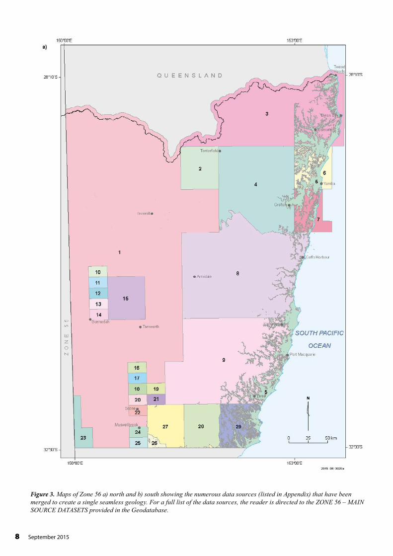
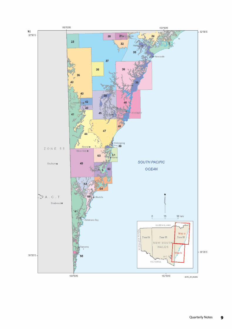
Data sourcesThe seamless geology dataset for UTM Zone 56 was compiled from 206 individual datasets representing published and unpublished GSNSW maps, thesis maps, journal publications, and unpublished maps from the GSNSW reports stored in DIGS (Figure 3). A list of the main data sources that refer to the numbered polygons in Figure 3 are provided in Appendix 1. For a full list of the data sources, the reader is directed to the ZONE 56 – MAIN SOURCE DATASETS provided

8 September 2015

Figure 3. Maps of Zone 56 a) north and b) south showing the numerous data sources (listed in Appendix) that have been merged to create a single seamless geology. For a full list of the data sources, the reader is directed to the ZONE 56 – MAIN SOURCE DATASETS provided in the Geodatabase.

9Quarterly Notes

10 September 2015

includes Woodburn 1:100 000 Geological Sheet, Bare Point 1:100 000 Geological Sheet, Warwick–Tweed Heads 1:250 000 Metallogenic Map, Manilla 1:100 000 Geological Sheet, Moss Vale 1:100 000 Geological Sheet and Gosford–Lake Macquarie 1:100 000 Geological Sheet. Another new dataset which has been integrated into the seamless geology of Zone 56 is a series of Quaternary coastal maps for the region between Newcastle and Wollongong (Troedson 2014).

Approach and methodologyGiven that all of the datasets used in the UTM Zone 56 geology database had to be formatted to adhere to the common structure used by the GSNSW Statewide Seamless Geology Project, the process of creating a seamless geology dataset for Zone 56 involved: (i) selecting the appropriate ‘best available’ datasets for different areas; (ii) updating georeferencing problems associated with mapping done using old base maps; (iii) dissolving map boundaries and dataset boundaries, including resolving edge-match and stratigraphic nomenclature conflicts between different maps and datasets; and (iv) interpreting the various layers under the cover of other layers.

Selecting the best available data depended on the generation and scale of mapping. For example, vector data from the more recent Warwick–Tweed Heads metallogenic map was used instead of the original geological maps that were compiled in the 1970s. Furthermore, mapping data collected at a better scale than that previously published by the GSNSW was converted into a vector data and merged with the surrounding maps. The detailed 1:25 000 maps of the southern Tamworth Belt (Roberts 2015), for example, are a primary example where higher resolution maps where merged with the surrounding 1:250 000 scale datasets (i.e. Tamworth–Hastings 1:250 000 Metallogenic Map).

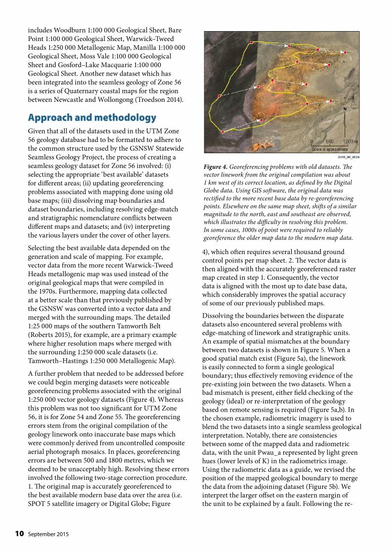
A further problem that needed to be addressed before we could begin merging datasets were noticeable georeferencing problems associated with the original 1:250 000 vector geology datasets (Figure 4). Whereas this problem was not too significant for UTM Zone 56, it is for Zone 54 and Zone 55. The georeferencing errors stem from the original compilation of the geology linework onto inaccurate base maps which were commonly derived from uncontrolled composite aerial photograph mosaics. In places, georeferencing errors are between 500 and 1800 metres, which we deemed to be unacceptably high. Resolving these errors involved the following two-stage correction procedure. 1. The original map is accurately georeferenced to the best available modern base data over the area (i.e. SPOT 5 satellite imagery or Digital Globe; Figure

4), which often requires several thousand ground control points per map sheet. 2. The vector data is then aligned with the accurately georeferenced raster map created in step 1. Consequently, the vector data is aligned with the most up to date base data, which considerably improves the spatial accuracy of some of our previously published maps.

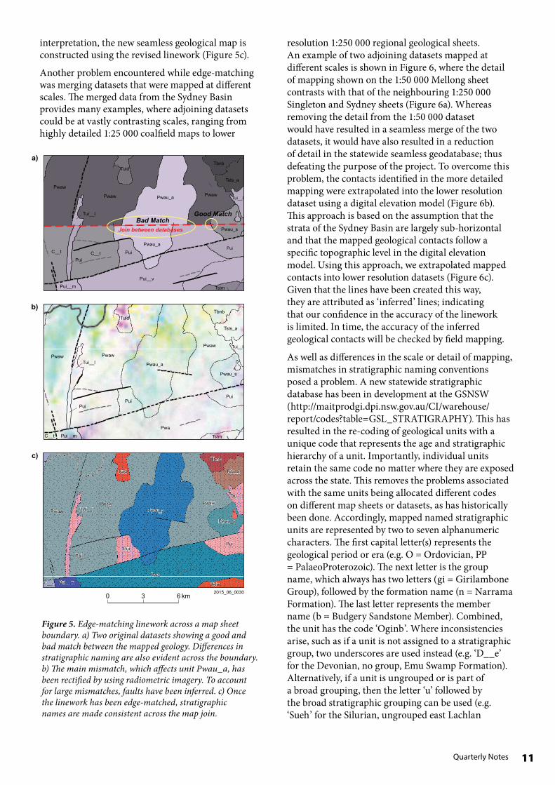
Dissolving the boundaries between the disparate datasets also encountered several problems with edge-matching of linework and stratigraphic units. An example of spatial mismatches at the boundary between two datasets is shown in Figure 5. When a good spatial match exist (Figure 5a), the linework is easily connected to form a single geological boundary; thus effectively removing evidence of the pre-existing join between the two datasets. When a bad mismatch is present, either field checking of the geology (ideal) or re-interpretation of the geology based on remote sensing is required (Figure 5a,b). In the chosen example, radiometric imagery is used to blend the two datasets into a single seamless geological interpretation. Notably, there are consistencies between some of the mapped data and radiometric data, with the unit Pwau_a represented by light green hues (lower levels of K) in the radiometrics image. Using the radiometric data as a guide, we revised the position of the mapped geological boundary to merge the data from the adjoining dataset (Figure 5b). We interpret the larger offset on the eastern margin of the unit to be explained by a fault. Following the re-

Figure 4. Georeferencing problems with old datasets. The vector linework from the original compilation was about 1 km west of its correct location, as defined by the Digital Globe data. Using GIS software, the original data was rectified to the more recent base data by re-georeferencing points. Elsewhere on the same map sheet, shifts of a similar magnitude to the north, east and southeast are observed, which illustrates the difficulty in resolving this problem. In some cases, 1000s of point were required to reliably georeference the older map data to the modern map data.

11Quarterly Notes

Figure 5. Edge-matching linework across a map sheet boundary. a) Two original datasets showing a good and bad match between the mapped geology. Differences in stratigraphic naming are also evident across the boundary. b) The main mismatch, which affects unit Pwau_a, has been rectified by using radiometric imagery. To account for large mismatches, faults have been inferred. c) Once the linework has been edge-matched, stratigraphic names are made consistent across the map join.

interpretation, the new seamless geological map is constructed using the revised linework (Figure 5c).

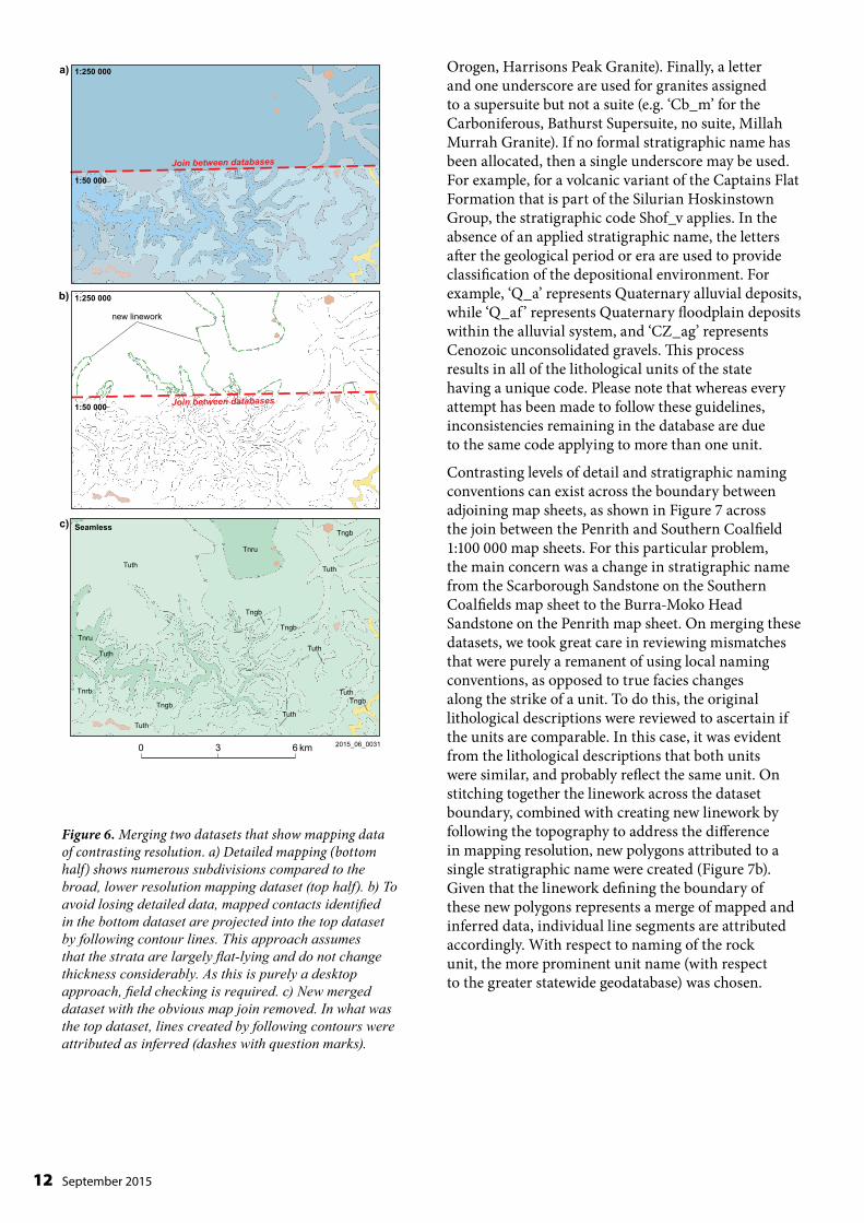
Another problem encountered while edge-matching was merging datasets that were mapped at different scales. The merged data from the Sydney Basin provides many examples, where adjoining datasets could be at vastly contrasting scales, ranging from highly detailed 1:25 000 coalfield maps to lower

Pwa

PwawPwaw Pwau_a

Pwaw

Pui

Tui__l

Pui

Tsts_a

Pwau_s

Tui__l

Pui

Tbnb

Tuid

TstmPui__mC__t

g

g

g

gg

o

o

Pwa

PwawPwaw

Pwau_a

Pwaw

PuiPui

Tsts_a

TbnbTuid

Pui

Tstm

Pwau_s

Tui__l

Pui__m

Tui__l

C__t

g

g

g

g

o

o

Bad MatchGood Match

Join between databases

Pui__v

C__tC__tPwau_a

PuiPui

TstmPui__m

Tui__l

Pwaw

Pwaw

Tuid

Pwau_a

Tbnb

Tsts_a

Tui__l

Pui

Pwau_s

Pwaw

2015_06_0030

a)

b)

c)

0 3 6 km

resolution 1:250 000 regional geological sheets. An example of two adjoining datasets mapped at different scales is shown in Figure 6, where the detail of mapping shown on the 1:50 000 Mellong sheet contrasts with that of the neighbouring 1:250 000 Singleton and Sydney sheets (Figure 6a). Whereas removing the detail from the 1:50 000 dataset would have resulted in a seamless merge of the two datasets, it would have also resulted in a reduction of detail in the statewide seamless geodatabase; thus defeating the purpose of the project. To overcome this problem, the contacts identified in the more detailed mapping were extrapolated into the lower resolution dataset using a digital elevation model (Figure 6b). This approach is based on the assumption that the strata of the Sydney Basin are largely sub-horizontal and that the mapped geological contacts follow a specific topographic level in the digital elevation model. Using this approach, we extrapolated mapped contacts into lower resolution datasets (Figure 6c). Given that the lines have been created this way, they are attributed as ‘inferred’ lines; indicating that our confidence in the accuracy of the linework is limited. In time, the accuracy of the inferred geological contacts will be checked by field mapping.

As well as differences in the scale or detail of mapping, mismatches in stratigraphic naming conventions posed a problem. A new statewide stratigraphic database has been in development at the GSNSW (http://maitprodgi.dpi.nsw.gov.au/CI/warehouse/report/codes?table=GSL_STRATIGRAPHY). This has resulted in the re-coding of geological units with a unique code that represents the age and stratigraphic hierarchy of a unit. Importantly, individual units retain the same code no matter where they are exposed across the state. This removes the problems associated with the same units being allocated different codes on different map sheets or datasets, as has historically been done. Accordingly, mapped named stratigraphic units are represented by two to seven alphanumeric characters. The first capital letter(s) represents the geological period or era (e.g. O = Ordovician, PP = PalaeoProterozoic). The next letter is the group name, which always has two letters (gi = Girilambone Group), followed by the formation name (n = Narrama Formation). The last letter represents the member name (b = Budgery Sandstone Member). Combined, the unit has the code ‘Oginb’. Where inconsistencies arise, such as if a unit is not assigned to a stratigraphic group, two underscores are used instead (e.g. ‘D__e’ for the Devonian, no group, Emu Swamp Formation). Alternatively, if a unit is ungrouped or is part of a broad grouping, then the letter ‘u’ followed by the broad stratigraphic grouping can be used (e.g. ‘Sueh’ for the Silurian, ungrouped east Lachlan

12 September 2015

Orogen, Harrisons Peak Granite). Finally, a letter and one underscore are used for granites assigned to a supersuite but not a suite (e.g. ‘Cb_m’ for the Carboniferous, Bathurst Supersuite, no suite, Millah Murrah Granite). If no formal stratigraphic name has been allocated, then a single underscore may be used. For example, for a volcanic variant of the Captains Flat Formation that is part of the Silurian Hoskinstown Group, the stratigraphic code Shof_v applies. In the absence of an applied stratigraphic name, the letters after the geological period or era are used to provide classification of the depositional environment. For example, ‘Q_a’ represents Quaternary alluvial deposits, while ‘Q_af ’ represents Quaternary floodplain deposits within the alluvial system, and ‘CZ_ag’ represents Cenozoic unconsolidated gravels. This process results in all of the lithological units of the state having a unique code. Please note that whereas every attempt has been made to follow these guidelines, inconsistencies remaining in the database are due to the same code applying to more than one unit.

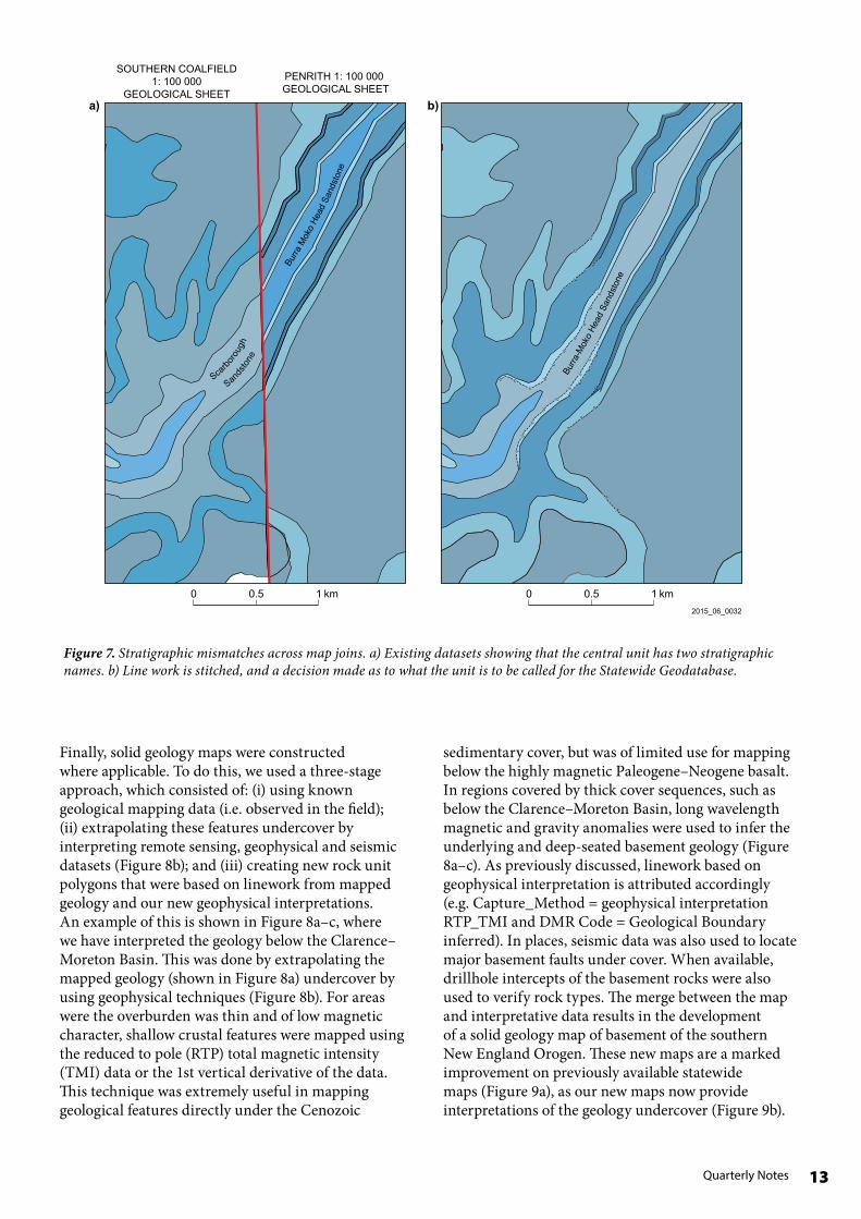
Contrasting levels of detail and stratigraphic naming conventions can exist across the boundary between adjoining map sheets, as shown in Figure 7 across the join between the Penrith and Southern Coalfield 1:100 000 map sheets. For this particular problem, the main concern was a change in stratigraphic name from the Scarborough Sandstone on the Southern Coalfields map sheet to the Burra-Moko Head Sandstone on the Penrith map sheet. On merging these datasets, we took great care in reviewing mismatches that were purely a remanent of using local naming conventions, as opposed to true facies changes along the strike of a unit. To do this, the original lithological descriptions were reviewed to ascertain if the units are comparable. In this case, it was evident from the lithological descriptions that both units were similar, and probably reflect the same unit. On stitching together the linework across the dataset boundary, combined with creating new linework by following the topography to address the difference in mapping resolution, new polygons attributed to a single stratigraphic name were created (Figure 7b). Given that the linework defining the boundary of these new polygons represents a merge of mapped and inferred data, individual line segments are attributed accordingly. With respect to naming of the rock unit, the more prominent unit name (with respect to the greater statewide geodatabase) was chosen.

Tngb

Tnru

Tuth

Tuth

Tnru

Tnrb

Tngb

Tngb

Tuth

Tngb

Tngb

Tuth

Tuth

TuthTuth

new linework

Join between databases

Join between databases

1:250 000

1:50 000

1:250 000

1:50 000

Seamless

2015_06_0031

c)

b)

a)

0 3 6 km

Figure 6. Merging two datasets that show mapping data of contrasting resolution. a) Detailed mapping (bottom half) shows numerous subdivisions compared to the broad, lower resolution mapping dataset (top half). b) To avoid losing detailed data, mapped contacts identified in the bottom dataset are projected into the top dataset by following contour lines. This approach assumes that the strata are largely flat-lying and do not change thickness considerably. As this is purely a desktop approach, field checking is required. c) New merged dataset with the obvious map join removed. In what was the top dataset, lines created by following contours were attributed as inferred (dashes with question marks).

13Quarterly Notes

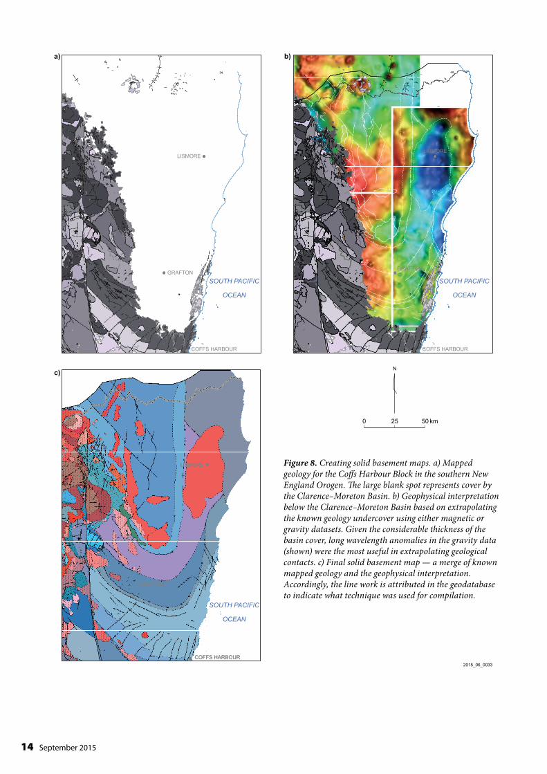
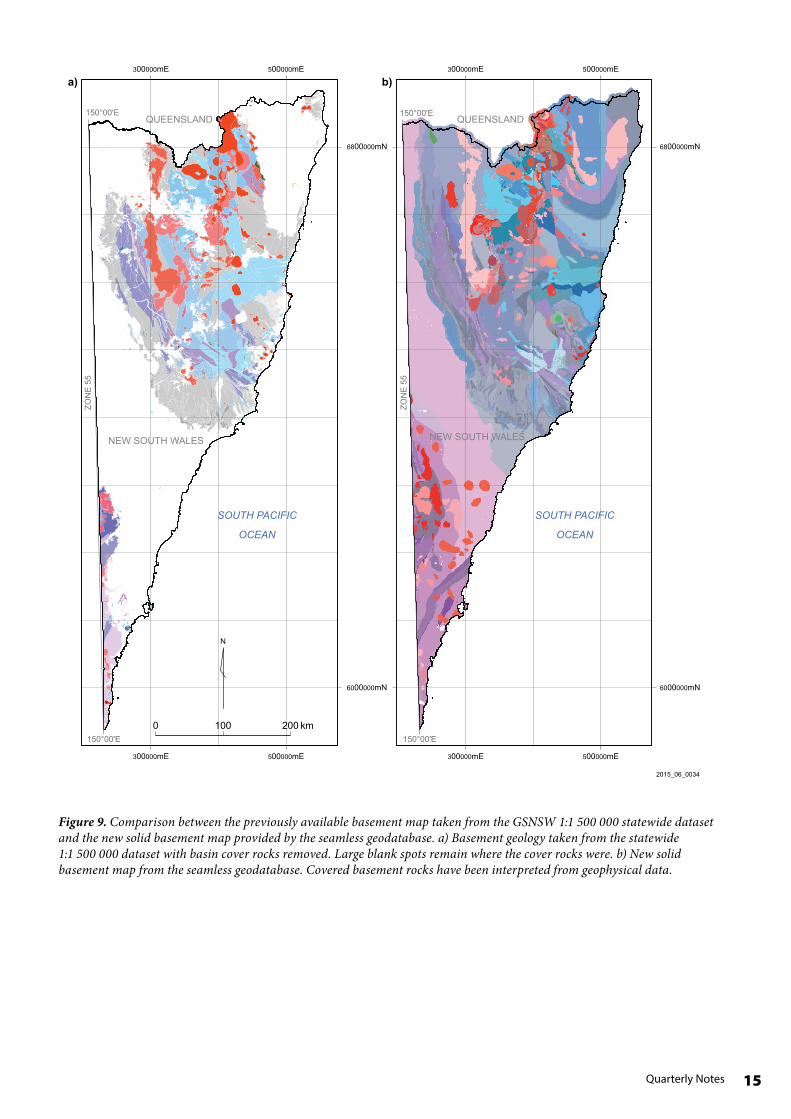
sedimentary cover, but was of limited use for mapping below the highly magnetic Paleogene–Neogene basalt. In regions covered by thick cover sequences, such as below the Clarence–Moreton Basin, long wavelength magnetic and gravity anomalies were used to infer the underlying and deep-seated basement geology (Figure 8a–c). As previously discussed, linework based on geophysical interpretation is attributed accordingly (e.g. Capture_Method = geophysical interpretation RTP_TMI and DMR Code = Geological Boundary inferred). In places, seismic data was also used to locate major basement faults under cover. When available, drillhole intercepts of the basement rocks were also used to verify rock types. The merge between the map and interpretative data results in the development of a solid geology map of basement of the southern New England Orogen. These new maps are a marked improvement on previously available statewide maps (Figure 9a), as our new maps now provide interpretations of the geology undercover (Figure 9b).

Finally, solid geology maps were constructed where applicable. To do this, we used a three-stage approach, which consisted of: (i) using known geological mapping data (i.e. observed in the field); (ii) extrapolating these features undercover by interpreting remote sensing, geophysical and seismic datasets (Figure 8b); and (iii) creating new rock unit polygons that were based on linework from mapped geology and our new geophysical interpretations. An example of this is shown in Figure 8a–c, where we have interpreted the geology below the Clarence–Moreton Basin. This was done by extrapolating the mapped geology (shown in Figure 8a) undercover by using geophysical techniques (Figure 8b). For areas were the overburden was thin and of low magnetic character, shallow crustal features were mapped using the reduced to pole (RTP) total magnetic intensity (TMI) data or the 1st vertical derivative of the data. This technique was extremely useful in mapping geological features directly under the Cenozoic

?

?

?

??

?

?

?

?

?

??

?

?

?

?

?

?

?

?

?

?

?

?

??

?

?

?

???

?

?

Burra

-Mok

o He

ad S

ands

tone

Burra

Mok

o He

ad S

ands

tone

Sca

rboro

ugh

Sands

tone

PENRITH 1: 100 000 GEOLOGICAL SHEET

SOUTHERN COALFIELD 1: 100 000

GEOLOGICAL SHEET

2015_06_0032

a) b)

0 0.5 1 km0 0.5 1 km

Figure 7. Stratigraphic mismatches across map joins. a) Existing datasets showing that the central unit has two stratigraphic names. b) Line work is stitched, and a decision made as to what the unit is to be called for the Statewide Geodatabase.

14 September 2015

SOUTH PACIFIC

OCEAN

LISMORE

COFFS HARBOUR

GRAFTON

g

g

g

g

g

g

g

g

g

g

g

g

g

g

gg

g

g

g

g

g

!!!!

!!

!!

!!

!!!!!!!!!!!! !!!!!!

MM MMM

M M

MM

M

M M

M

M MM MM M

M

FFFFFFF

F

MM

g

g

g

g

g

g

g

g

g

g

g

g

g

g

gg

g

g

g

g

g

g

g

g

g

g

g

g

g

g

g

g

gg

g

g

g

gg

g

g

g

g

g

g

g

g

g

g

g

g

g

g

g

g

g

g

g

g

gg

g

gg

g

gg

g

g

g

g

g

g

gg

gg

g

gg

g

g

g

##

g

g

g

g

LISMORE

COFFS HARBOUR

GRAFTON

LISMORE

COFFS HARBOUR

GRAFTON

SOUTH PACIFIC

OCEAN

g

g

g

g

g

g

g

g

g

g

g

g

g

g

gg

g

g

g

g

g

!!!!

!!

!!

!!

!!

!!!!!! !!!!!!!!!!!!!!!! !!!!!!

MM MMM

M M

MM

M

M M

M

M MM MM M

M

FFFFFFF

F

MM

LISMORE

COFFS HARBOUR

GRAFTON

SOUTH PACIFIC

OCEAN

0 25 50 km

2015_06_0033

a)

c)

b)

Figure 8. Creating solid basement maps. a) Mapped geology for the Coffs Harbour Block in the southern New England Orogen. The large blank spot represents cover by the Clarence–Moreton Basin. b) Geophysical interpretation below the Clarence–Moreton Basin based on extrapolating the known geology undercover using either magnetic or gravity datasets. Given the considerable thickness of the basin cover, long wavelength anomalies in the gravity data (shown) were the most useful in extrapolating geological contacts. c) Final solid basement map — a merge of known mapped geology and the geophysical interpretation. Accordingly, the line work is attributed in the geodatabase to indicate what technique was used for compilation.

15Quarterly Notes

QUEENSLAND

NEW SOUTH WALES

SOUTH PACIFIC

OCEAN

300000mE 500000mE

300000mE 500000mE

6800000mN

6000000mN

ZON

E 5

5

150°00'E

150°00'EQUEENSLAND

NEW SOUTH WALES

SOUTH PACIFIC

OCEAN

300000mE 500000mE

300000mE 500000mE

6800000mN

6000000mN

150°00'E

150°00'E

ZON

E 5

5

2015_06_0034

a) b)

0 100 200 km

Figure 9. Comparison between the previously available basement map taken from the GSNSW 1:1 500 000 statewide dataset and the new solid basement map provided by the seamless geodatabase. a) Basement geology taken from the statewide 1:1 500 000 dataset with basin cover rocks removed. Large blank spots remain where the cover rocks were. b) New solid basement map from the seamless geodatabase. Covered basement rocks have been interpreted from geophysical data.

16 September 2015

ApplicationsIn this section, we present three potential applications of the seamless geology database of UTM Zone 56. These applications are: examining basement-cover relationships; using the geodatabase as a spatial search engine; and generating maps for a chosen area and/or geological domain.

Due to the structure of the seamless geodatabase, individual geological layers can be switched on or off. This feature allows the geological character of a particular area to be viewed, from the surface map (exposed) geology all the way down to the solid basement map. For example, if a review of the basement–cover relationships between a basin and basement is required, then all of the overlying younger rock data can be removed from the viewer. Alternatively, if knowledge of a Quaternary drainage system is important and the detail provided by the underlying geology is not required, then only the Cenozoic cover can be shown in the map viewer. Thus the functionality of the geodatabase allows any individual or particular combination of geological layers to be switched ‘on’ or ‘off’.

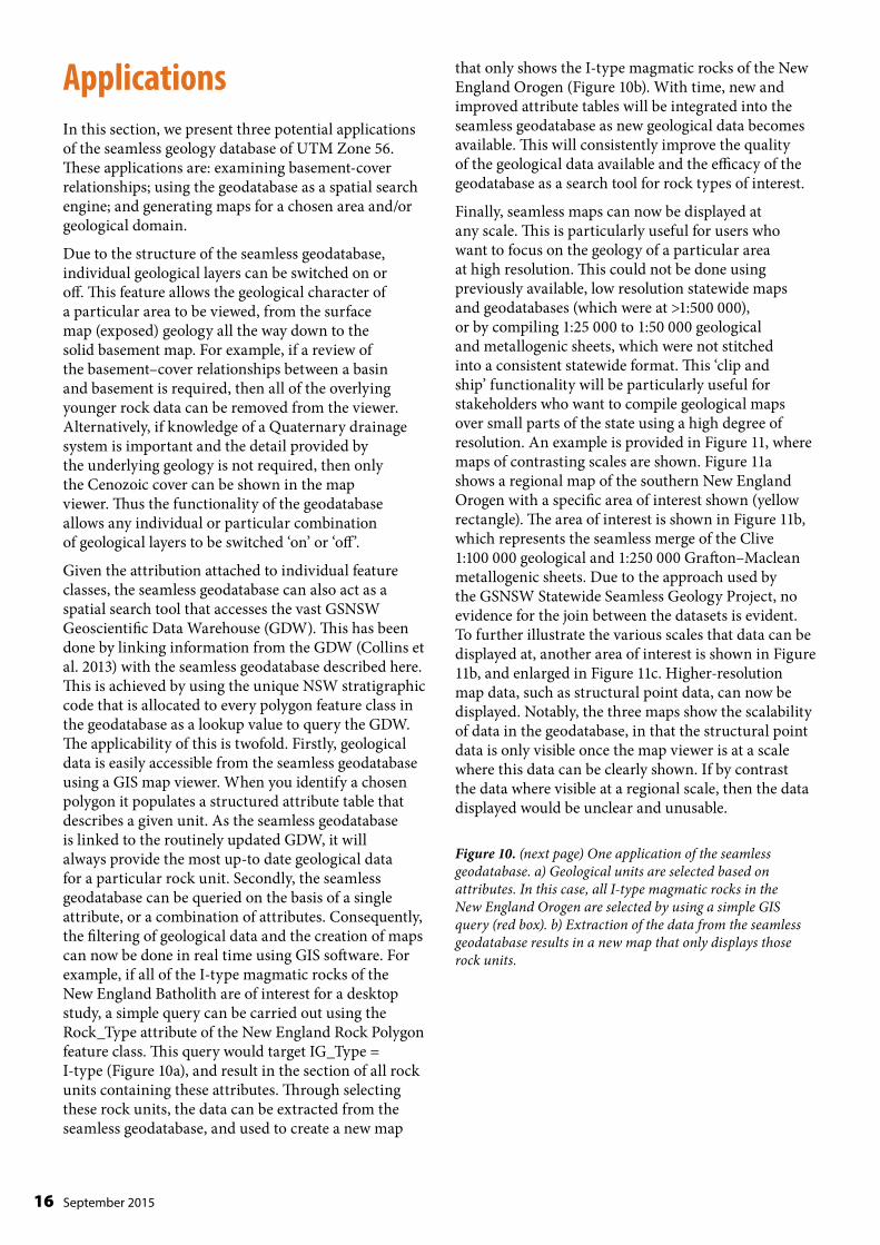
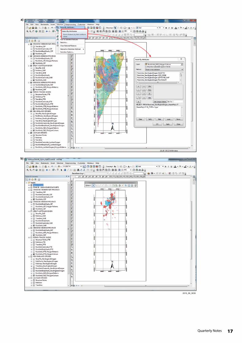
Given the attribution attached to individual feature classes, the seamless geodatabase can also act as a spatial search tool that accesses the vast GSNSW Geoscientific Data Warehouse (GDW). This has been done by linking information from the GDW (Collins et al. 2013) with the seamless geodatabase described here. This is achieved by using the unique NSW stratigraphic code that is allocated to every polygon feature class in the geodatabase as a lookup value to query the GDW. The applicability of this is twofold. Firstly, geological data is easily accessible from the seamless geodatabase using a GIS map viewer. When you identify a chosen polygon it populates a structured attribute table that describes a given unit. As the seamless geodatabase is linked to the routinely updated GDW, it will always provide the most up-to date geological data for a particular rock unit. Secondly, the seamless geodatabase can be queried on the basis of a single attribute, or a combination of attributes. Consequently, the filtering of geological data and the creation of maps can now be done in real time using GIS software. For example, if all of the I-type magmatic rocks of the New England Batholith are of interest for a desktop study, a simple query can be carried out using the Rock_Type attribute of the New England Rock Polygon feature class. This query would target IG_Type = I-type (Figure 10a), and result in the section of all rock units containing these attributes. Through selecting these rock units, the data can be extracted from the seamless geodatabase, and used to create a new map

that only shows the I-type magmatic rocks of the New England Orogen (Figure 10b). With time, new and improved attribute tables will be integrated into the seamless geodatabase as new geological data becomes available. This will consistently improve the quality of the geological data available and the efficacy of the geodatabase as a search tool for rock types of interest.

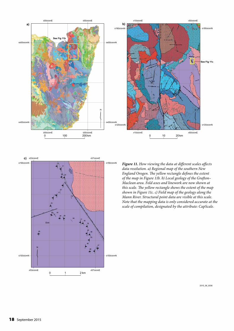
Finally, seamless maps can now be displayed at any scale. This is particularly useful for users who want to focus on the geology of a particular area at high resolution. This could not be done using previously available, low resolution statewide maps and geodatabases (which were at >1:500 000), or by compiling 1:25 000 to 1:50 000 geological and metallogenic sheets, which were not stitched into a consistent statewide format. This ‘clip and ship’ functionality will be particularly useful for stakeholders who want to compile geological maps over small parts of the state using a high degree of resolution. An example is provided in Figure 11, where maps of contrasting scales are shown. Figure 11a shows a regional map of the southern New England Orogen with a specific area of interest shown (yellow rectangle). The area of interest is shown in Figure 11b, which represents the seamless merge of the Clive 1:100 000 geological and 1:250 000 Grafton–Maclean metallogenic sheets. Due to the approach used by the GSNSW Statewide Seamless Geology Project, no evidence for the join between the datasets is evident. To further illustrate the various scales that data can be displayed at, another area of interest is shown in Figure 11b, and enlarged in Figure 11c. Higher-resolution map data, such as structural point data, can now be displayed. Notably, the three maps show the scalability of data in the geodatabase, in that the structural point data is only visible once the map viewer is at a scale where this data can be clearly shown. If by contrast the data where visible at a regional scale, then the data displayed would be unclear and unusable.

Figure 10. (next page) One application of the seamless geodatabase. a) Geological units are selected based on attributes. In this case, all I-type magmatic rocks in the New England Orogen are selected by using a simple GIS query (red box). b) Extraction of the data from the seamless geodatabase results in a new map that only displays those rock units.

17Quarterly Notes

2015_06_0035

a)

b)

18 September 2015

6750000mN

453000mE 457000mE

453000mE 457000mE

6756000mN

6750000mN

6756000mN

0 1 2 km

6720000mN

410000mE 450000mE

410000mE 450000mE

6790000mN

6720000mN

6790000mN

See Fig 11c

0 10 20km0 100 200km

See Fig 11b

6400000mN

300000mE 500000mE

300000mE 500000mE

6800000mN

6400000mN

6800000mN

2015_06_0036

a)

c)

b)

Figure 11. How viewing the data at different scales affects data resolution. a) Regional map of the southern New England Orogen. The yellow rectangle defines the extent of the map in Figure 11b. b) Local geology of the Grafton–Maclean area. Fold axes and linework are now shown at this scale. The yellow rectangle shows the extent of the map shown in Figure 11c. c) Field map of the geology along the Mann River. Structural point data are visible at this scale. Note that the mapping data is only considered accurate at the scale of compilation, designated by the attribute: CapScale.

19Quarterly Notes

ReferencesTroedson A., Hashimoto R., Jaworska J., Malloch K., Cain L. 2004. New South Wales Coastal Quaternary Geology Digital Data Set. NSW Department of Primary Industries, Mineral Resources, for Comprehensive Coastal Assessment.

Collins D.B., Gilmore P.J., Greenfield J.E. & Barlin T.R. 2013. The Geoscientific Data Warehouse – delivering NSW geoscience data. Quarterly Notes of the Geological Survey of New South Wales 139, 1–22.

Dawson M., Vickery N., Barnes R.G., & Mcdonald K. 2003. Compiled & interpreted geological dataset of the Nandewar Western regional Assessment area, northern NSW. Digital dataset, GSNSW, NSW Department of Mineral Resources, Sydney.

Roberts J. 2015. Preliminary 1:25 000 geological maps of the New England Orogen. Geological Survey of New South Wales, File 2015/1123.

Troedson A.L. 2014. Coastal Quaternary geology mapping: Filling the Newcastle to Wollongong gap. NSW Coastal Conference 2014 proceedings. url: http://www.coastalconference.com/2014/papers2014/Alexa%20Troedson%20Full%20Paper.pdf.

Troedson A.L. & Hashimoto T.R. 2008. Coastal Quaternary Geology — north and south coast of NSW. Geological Survey of New South Wales, Bulletin 34.

ConclusionThe GSNSW SSGP aims to produce a dynamic geological model of the state of NSW by merging best-available mapping data that has been converted into a statewide, consistent format. While this article describes the approach and methodology used for compiling a geodatabase for the geology of UTM Zone 56, the same methods will be used for Zone 54 and Zone 55. The main steps used in compiling the database involved identifying the best-available mapping data and converting the data into the new statewide consistent format, updating georeferencing problems inherited from older maps, dissolving map boundaries and geological conflicts through edge mapping line work and harmonising stratigraphic naming conventions and finally, interpreting geology undercover to create solid geology maps. The resulting geodatabase is a fully scalable dynamic model of NSW geology that can be interrogated spatially or by searching for attributes that are linked to all feature classes. Through exporting the data, maps showing the query results can be readily created using GIS software.

AcknowledgementsThe authors would like to acknowledge the many geologists and cartographers from the GSNSW who have worked on the constituent datasets of the NSW UTM Zone 56 seamless geology over the past 40 or more years. Significant contributors included many of the geologists from the former Armidale office (Bob Brown, Jim Stroud, Rob Barnes, Harvey Henley, Joan Henley, Jeff Brownlow, Mark Dawson, Nancy Vickery and Frances Spiller) and cartography staff (Ken McDonald and Phil Kennedy). We would also like to acknowledge Joel Fitzherbert for compiling the solid geology Lachlan data layer and James Ballard for assigning rock unit codes and data compilation. The detailed compilations of Carboniferous geology of the Tamworth Belt by John Roberts (formerly University of NSW) also significantly enhanced the existing published geological coverage over many areas. The Quaternary coastal geology dataset (Troedson et al. 2004) was the product of a team of GSNSW geologists including Alexa Troedson, Riko Hashimoto, Jola Jaworska, Kirstine Malloch and Llew Cain. John Greenfield is acknowledged for initial concept development and ongoing support of the project. Mark Dawson (Whitehaven Coal Ltd) is thanked for providing a thorough review of the Zone 56 seamless geology digital dataset. Suggestions made by Phil Gilmore also lead to significant improvements to the paper.

20 September 2015

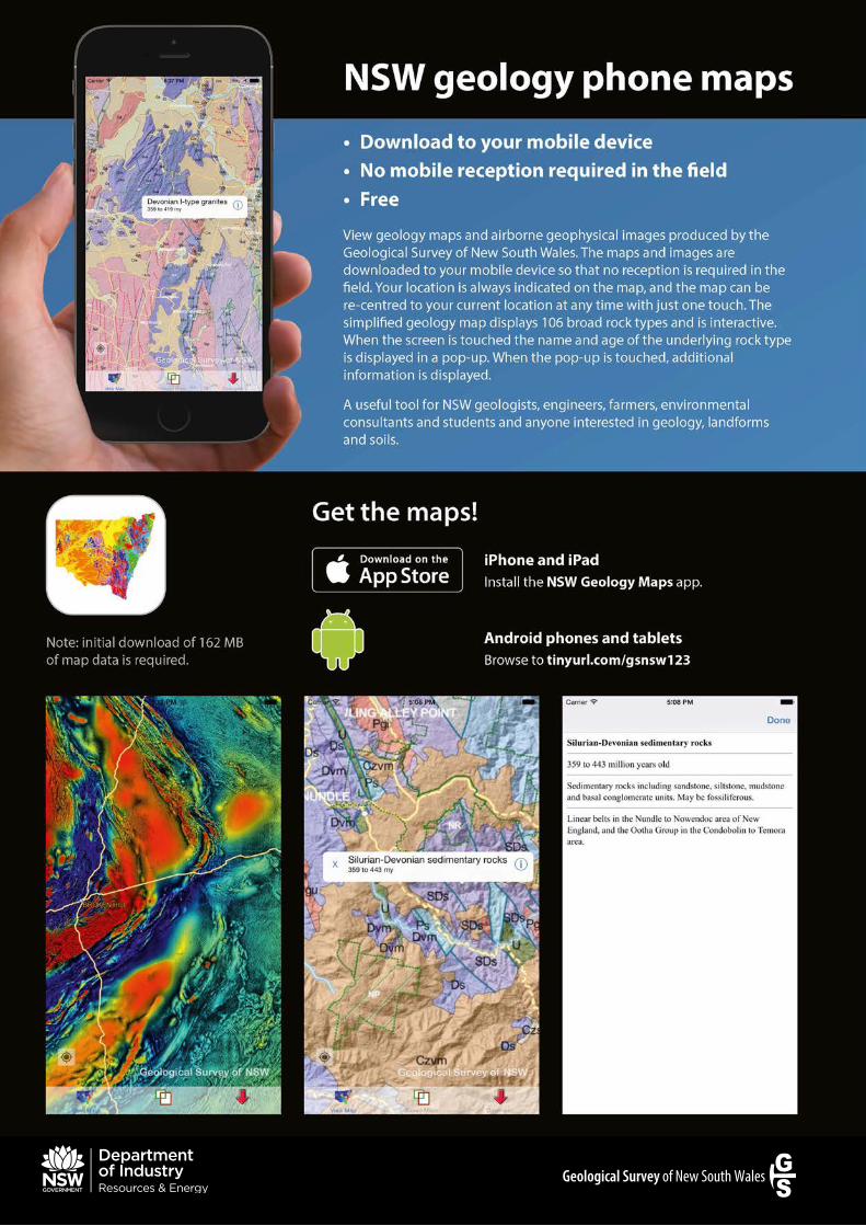
Mobile seamless geologyKyle S. Hughes & James C. Ballard

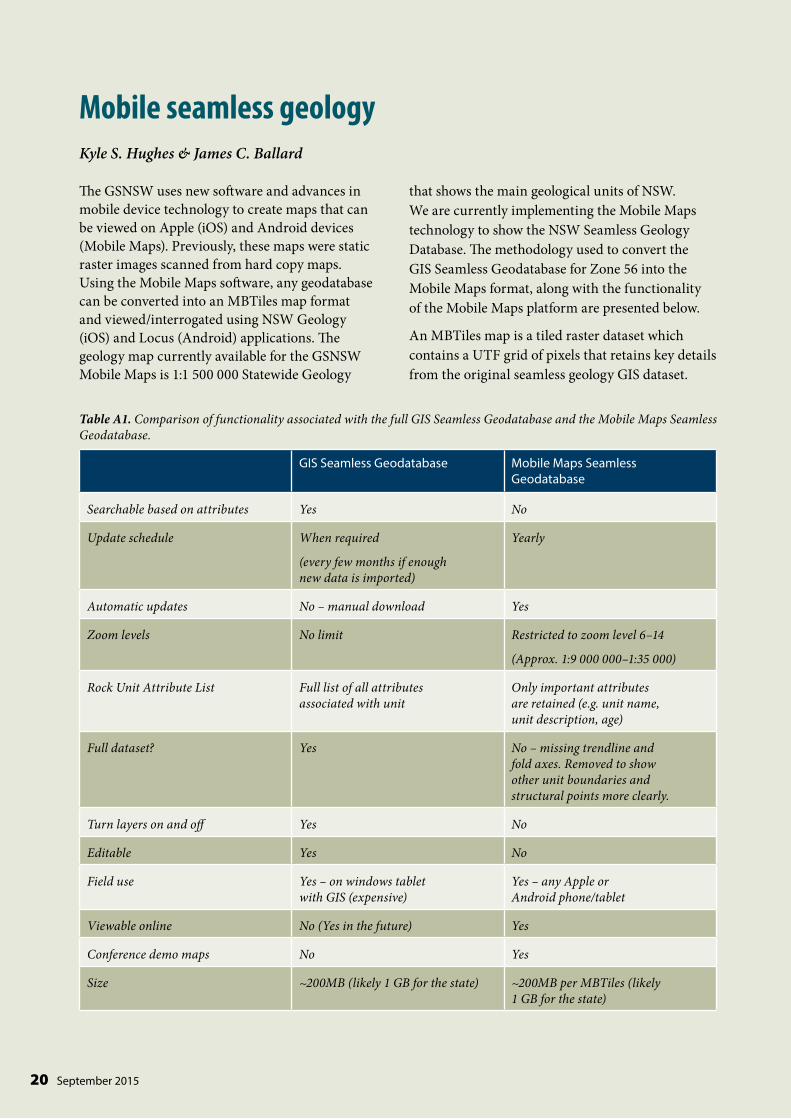
Table A1. Comparison of functionality associated with the full GIS Seamless Geodatabase and the Mobile Maps Seamless Geodatabase.

GIS Seamless Geodatabase Mobile Maps Seamless Geodatabase

Searchable based on attributes Yes No

Update schedule When required

(every few months if enough new data is imported)

Yearly

Automatic updates No – manual download Yes

Zoom levels No limit Restricted to zoom level 6–14

(Approx. 1:9 000 000–1:35 000)

Rock Unit Attribute List Full list of all attributes associated with unit

Only important attributes are retained (e.g. unit name, unit description, age)

Full dataset? Yes No – missing trendline and fold axes. Removed to show other unit boundaries and structural points more clearly.

Turn layers on and off Yes No

Editable Yes No

Field use Yes – on windows tablet with GIS (expensive)

Yes – any Apple or Android phone/tablet

Viewable online No (Yes in the future) Yes

Conference demo maps No Yes

Size ~200MB (likely 1 GB for the state) ~200MB per MBTiles (likely 1 GB for the state)

The GSNSW uses new software and advances in mobile device technology to create maps that can be viewed on Apple (iOS) and Android devices (Mobile Maps). Previously, these maps were static raster images scanned from hard copy maps. Using the Mobile Maps software, any geodatabase can be converted into an MBTiles map format and viewed/interrogated using NSW Geology (iOS) and Locus (Android) applications. The geology map currently available for the GSNSW Mobile Maps is 1:1 500 000 Statewide Geology

that shows the main geological units of NSW. We are currently implementing the Mobile Maps technology to show the NSW Seamless Geology Database. The methodology used to convert the GIS Seamless Geodatabase for Zone 56 into the Mobile Maps format, along with the functionality of the Mobile Maps platform are presented below.

An MBTiles map is a tiled raster dataset which contains a UTF grid of pixels that retains key details from the original seamless geology GIS dataset.

21Quarterly Notes

Accordingly, important attribute data such as unit name, geological description, age, depositional environment and the geological province can be attached to geological units in the Mobile Maps environment. However, unlike the full GIS version of the seamless geodatabase, it is not possible to search and select based on these attributes. The stratigraphic boundaries and units in the Mobile Maps version will be exactly the same as for the GIS Seamless Geodatabase. The only feature classes missing from the Mobile Maps geodatabase are trend lines and fold axes. This was done so that important feature classes such as structural point data can be viewed without obstruction. It is important to note that all symbology used for the GIS Seamless Geodatabase is closely matched in the MBTiles file (using CartoCSS). A comparison of the GIS Seamless Geodatabase and the Mobile Maps Seamless Geodatabase is shown in Table A1.

Significantly, the ability to show the seamless geodatabase using Mobile Maps technology means that anyone can access the geodatabase for free (or very cheaply given that Android tablets with GPS can be as little as $100). This allows anyone

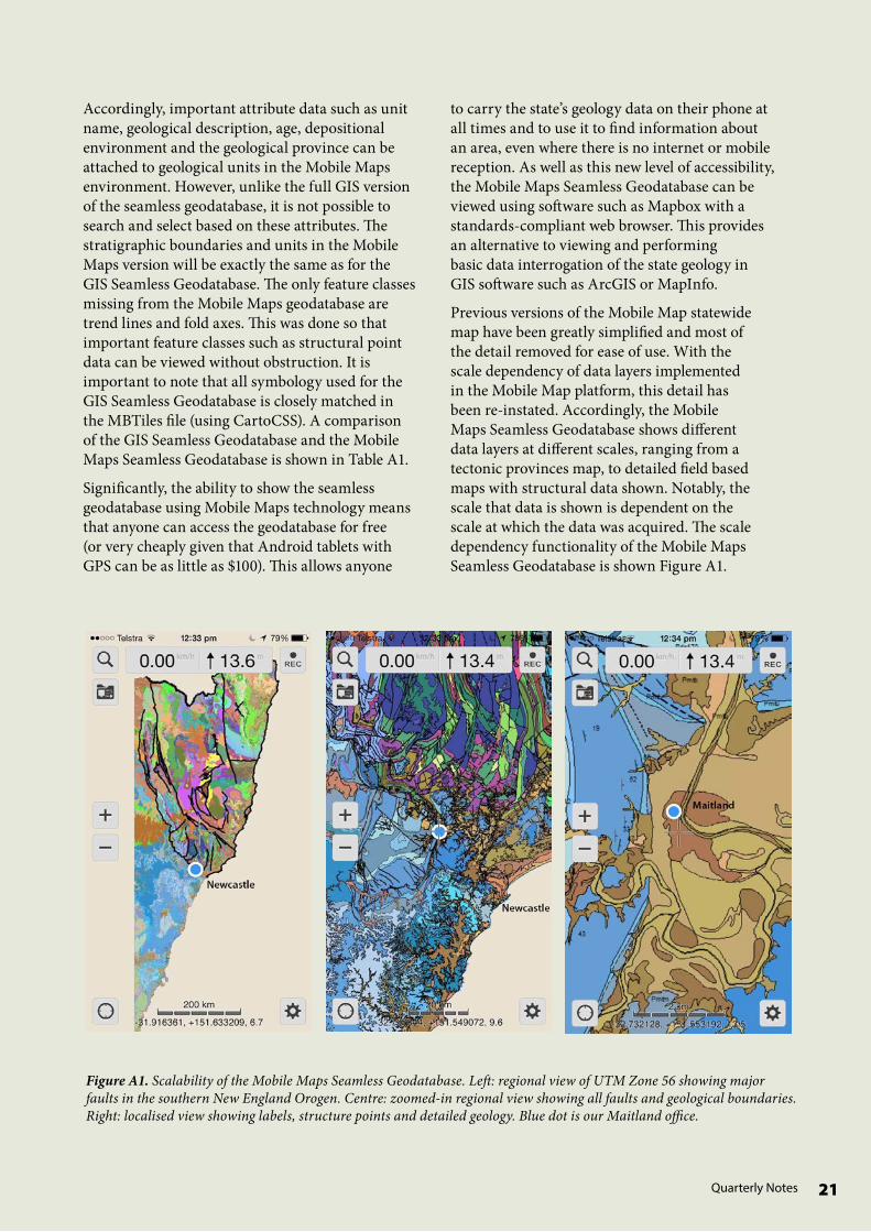
Figure A1. Scalability of the Mobile Maps Seamless Geodatabase. Left: regional view of UTM Zone 56 showing major faults in the southern New England Orogen. Centre: zoomed-in regional view showing all faults and geological boundaries. Right: localised view showing labels, structure points and detailed geology. Blue dot is our Maitland office.

to carry the state’s geology data on their phone at all times and to use it to find information about an area, even where there is no internet or mobile reception. As well as this new level of accessibility, the Mobile Maps Seamless Geodatabase can be viewed using software such as Mapbox with a standards-compliant web browser. This provides an alternative to viewing and performing basic data interrogation of the state geology in GIS software such as ArcGIS or MapInfo.

Previous versions of the Mobile Map statewide map have been greatly simplified and most of the detail removed for ease of use. With the scale dependency of data layers implemented in the Mobile Map platform, this detail has been re-instated. Accordingly, the Mobile Maps Seamless Geodatabase shows different data layers at different scales, ranging from a tectonic provinces map, to detailed field based maps with structural data shown. Notably, the scale that data is shown is dependent on the scale at which the data was acquired. The scale dependency functionality of the Mobile Maps Seamless Geodatabase is shown Figure A1.

22 September 2015

Figure A2. Screenshots of Mobile Maps Seamless Geodatabase data showing the standard map viewer with: (top) first-tap functionality, and (bottom) second-tap functionality and a simplified attribute table.

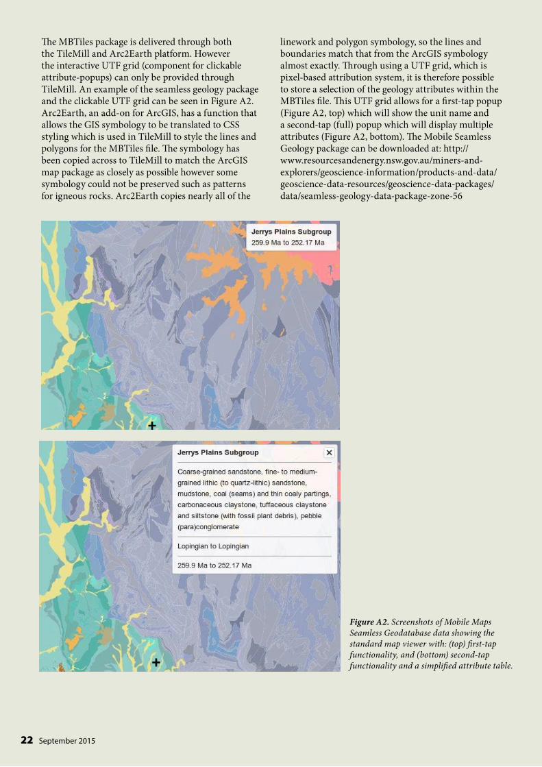
The MBTiles package is delivered through both the TileMill and Arc2Earth platform. However the interactive UTF grid (component for clickable attribute-popups) can only be provided through TileMill. An example of the seamless geology package and the clickable UTF grid can be seen in Figure A2. Arc2Earth, an add-on for ArcGIS, has a function that allows the GIS symbology to be translated to CSS styling which is used in TileMill to style the lines and polygons for the MBTiles file. The symbology has been copied across to TileMill to match the ArcGIS map package as closely as possible however some symbology could not be preserved such as patterns for igneous rocks. Arc2Earth copies nearly all of the

linework and polygon symbology, so the lines and boundaries match that from the ArcGIS symbology almost exactly. Through using a UTF grid, which is pixel-based attribution system, it is therefore possible to store a selection of the geology attributes within the MBTiles file. This UTF grid allows for a first-tap popup (Figure A2, top) which will show the unit name and a second-tap (full) popup which will display multiple attributes (Figure A2, bottom). The Mobile Seamless Geology package can be downloaded at: http://www.resourcesandenergy.nsw.gov.au/miners-and-explorers/geoscience-information/products-and-data/geoscience-data-resources/geoscience-data-packages/data/seamless-geology-data-package-zone-56

23Quarterly Notes

Source

1 Dawson M., Vickery N., Barnes R.G., & Mcdonald K. 2003. Compiled & interpreted geological dataset of the Nandewar Western regional Assessment area, northern NSW. Digital dataset, GSNSW, NSW Department of Mineral Resources, Sydney.

2 Henley H.F., Brown R.E. & Brownlow 2000. Clive 1:100 000 Geological Sheet 9239. GSNSW, Sydney.

3 Brown R.E., Cranfield L.C., Denaro T.J., Burrows P.E., Henley H.F., Stroud W.J. & Brownlow J.W. 2007. Warwick–Tweed Heads 1:250 000 Metallogenic Map (Provisional) SH/56-02 and 03. Geological Survey of NSW/Geological Survey of Qld.

4 Henley H.F., Brown R.E., Brownlow J.W., Barnes R.G. & Stroud W.J. 2001. Grafton–Maclean 1:250 000 Metallogenic Map. GSNSW, Sydney.

5 Troedson A., Hashimoto R., Jaworska J., Malloch K., Cain L. 2004. New South Wales Coastal Quaternary Geology Digital Data Set. NSW Department of Primary Industries, Mineral Resources, for Comprehensive Coastal Assessment.

6 Brownlow J.W. 2002. Woodburn 1:100 000 Geological Sheet 8539. GSNSW, Sydney.

7 Brownlow J.W. 2003. Bare Point 1:100 000 Geological Sheet 9538, provisional edition. GSNSW, Sydney.

8 Gilligan L.B., Brownlow J.W., Cameron R.G. & Henley H.F. 1992. Dorrigo–Coffs Harbour 1:250 000 Metallogenic Map. GSNSW, Sydney.

9 Gilligan L.B., Brownlow J.W. & Cameron R.G. 1987. Tamworth–Hastings 1:250 000 Metallogenic Map. GSNSW, Sydney.

10 Roberts J. 2002. Preliminary geology of the Plagyn 1:25000 map sheet. University of NSW, GSNSW report GS2015/1123.

11 Roberts J. 2002. Preliminary geology of the Berrioye 1:25000 map sheet. University of NSW, GSNSW report GS2015/1123.

12 Roberts J. 2002. Preliminary geology of the Willuri 1:25000 Map sheet. University of NSW, GSNSW report GS2015/1123.

13 Roberts J. 2002. Preliminary geology of the Kelvin 1:25000 map sheet. University of NSW, GSNSW report GS2015/1123.

14 Roberts J. 2002. Preliminary geology of the Gunnedah 1:250000 map sheet. University of NSW, GSNSW report GS2015/1123.

15 Brown R.E., Henley H.F., Vickery N.M., Glen R.A. & Stroud W.J. 2012. Manilla 1:100 000 Geological Sheet 9036. Geological Survey of NSW, Armidale.

16 Roberts J. 2001. Geological Compilation dyeline. Wallabadah 1:25 000 sheet 9034-I-N. University of NSW, GSNSW report GS2015/1123.

Appendix: Data sources for UTM Zone 56

24 September 2015

17 Roberts J. 2001. Geological Compilation dyeline. Temi 1:25 000 sheet 9034-I-S. University of NSW, GSNSW report GS2015/1123.

18 Roberts J. 2001. Geological Compilation dyeline. Murrurundi 1:25 000 sheet 9034-II-N. University of NSW, GSNSW report GS2015/1123.

19 Roberts J. 2001. Geological Compilation dyeline. Timor 1:25 000 sheet 9134-III-N. University of NSW, GSNSW report GS2015/1123.

20 Roberts J. 2001. Geological Compilation dyeline. Parkville 1:25 000 sheet 9034-II-S. University of NSW, GSNSW report GS2015/1123.

21 Roberts J. 2001. Geological Compilation dyeline. Waverly 1:25 000 sheet 9134-III-S. University of NSW, GSNSW report GS2015/1123.

22 Roberts J. 2001. Geological Compilation dyeline. Scone 1:25 000 sheet 9033-I-N. University of NSW, GSNSW report GS2015/1123.

23 Yoo E.K. 1998. Western Coalfield Regional Geology (Northern Part) 1:100 000. GSNSW, Sydney.

24 Summerhayes G. 1983. Muswellbrook 1:25 000 Geological Map, 9033-II-N, GSNSW, Sydney.

25 Sniffin M.J. & Summerhayes G.J. 1985. Jerrys Plains 1:25 000 Geological Sheet 9033-II-S. GSNSW, Sydney.

26 Glen R.A. & Beckett J. 1993. Hunter Coalfield Regional Geology 1:100 000, 2nd edition. GSNSW, Sydney. Modified by the Nandewar Regional Assessment dataset, 2003.

27 Roberts J., Engel B. & Chapman J. (editor) 1991. Camberwell 1:100 000 Geological Sheet 9133. GSNSW, Sydney.

28 Roberts J., Engel B., Lennox M. & Chapman J. (editor) 1991. Dungog 1:100 000 Geological Sheet 9233. GSNSW, Sydney.

29 Engel B., Roberts J, Roy P.S. & Chapman J. (editor) 1991. Bulahdelah 1:100 000 Geological Sheet 9333. GSNSW, Sydney.

30 Sniffin M.J., Mcilveen G.R., & Crouch A. 1988. Doyles Creek 1:25 000 Geological Sheet 9032-1-N. GSNSW, Sydney

31 McILVEEN G.R. 1984. Singleton 1:25 000 Geological Sheet 9132-IV-N. GSNSW, Sydney.

32 Glen R.A. & Beckett J. 1993. Hunter Coalfield Regional Geology 1:100 000, 2nd edition. GSNSW, Sydney.

33 Hawley S.P., Glen R.A. & Baker C.J. 1995. Newcastle Coalfield Regional Geology 1:100 000. GSNSW, Sydney.

34 Rose G., Jones W.H. & Kennedy D.R. 1966. Newcastle 1:250 000 Geological Sheet SI/56-02, 1st edition, GSNSW, Sydney.

35 Yoo E.K. 1992. Western Coalfield Regional Geology (southern part) 1:100 000, 1st edition. GSNSW, Sydney.

36 Goldberry R. 1969. Mellong 1:50 000 Geological Map, 9031-IV, GSNSW, Sydney.

25Quarterly Notes

37 Singleton & Sydney 1:250 000 geological maps. Modified by the Lower Northeast Regional Forestry Assessment, 1999.

38 Och D.J., Jones D.C., Uren R.E. & Hughes K.S. 2015. Gosford–Lake Macquarie 1:100 000 Geological Sheet 9131 & 9231. GSNSW, Maitland.

39 Troedson A. 2014. Newcastle to Wollongong Coastal Quaternary Mapping, digital dataset. Compiled for the GSNSW as part of the Seamless Geology Project.

40 Bryan J.H. 1966. Sydney 1:250 000 Geological Sheet SI/56-05, 3rd edition, GSNSW, Sydney. Modified by the Lower Northeast Regional Forestry Assessment dataset, 1999.

41 Glen R.A., Dawson M.W., & Colquhoun G.P. 2007. Eastern Lachlan Orogen Geoscience Database (on DVD-ROM) Version 2. GSNSW, Department of Primary Industries, Maitland.

42 Goldberry R. & Bembrick C.S. 1996. Katoomba 1:50 000 Geological Map, 8930-I, Prov. 1st ed. GSNSW, Sydney.

43 Authors Unknown 1969. Jamison 1:50 000 Geological Map 8930-2, Prov. 1st ed. GSNSW, Sydney (unpublished).

44 Moffitt R.S. 1999. Southern Coalfield Regional Geology 1:100 000. GSNSW, Sydney.

45 Clark N.R. & Jones D.C. 1991. Penrith 1:100 000 Geological Sheet 9030. GSNSW, Sydney.

46 Herbert C. 1983. Sydney 1:100 000 Geological Sheet 9130. GSNSW, Sydney.

47 Stroud W.J., Sherwin L., Roy H.N. & Baker C.J. 1985. Wollongong–Port Hacking 1:100 000 Geological Sheet 9029-9129, 1st edition. GSNSW, Sydney.

48 Stroud W.J., Sherwin L., Roy H.N. & Baker C.J. 1985. Wollongong – Port Hacking 1:100 000 Geological Sheet 9029–9129. GSNSW, Sydney.

49 Trigg S.J. & Campbell L.M. 2012. Moss Vale 1:100 000 Geological Sheet 8928 (Provisional). GSNSW, Maitland

50 Bowman H.N. 1974. Robertson 1:50 000 Geological Map, 9028-IV, GSNSW, Sydney.

51 Bowman H.N. 1974. Kiama 1:50 000 Geological Map, 9028-I, GSNSW, Sydney.

52 Bowman H.N 1972. Nowra–Toolijooa 1:50 000 Geological Map 9028-2 & 9028-3 (part), Prov. 1st ed. GSNSW, Sydney (unpublished).

53 Mcilveen G. 1974. Ulladulla 1:250 000 Metallogenic Map. GSNSW, Sydney. Modified by the RACAC Southern dataset, 2000.

54 Paterson I.B.L. 1975. Jervis Bay and Currarong 1:50 000 Geological Map 7265, GSNSW, Sydney.

55 Mcilveen G.. 1973. Ulladulla 1:250 000 Metallogenic Sheet. GSNSW, Sydney.

56 Lewis P.C. & Glen R.A. 1995. Bega–Mallacoota 1:250 000 Geological Sheet SJ/55-04 & part SJ/55-08, 2nd edition. GSNSW, Sydney.

*GSNSW = Geological Survey of New South Wales

26 September 2015

27Quarterly Notes

NSW Department of Industry, Division of Resources & Energy516 High Street, Maitland NSW 2320PO Box 344 Hunter Region Mail Centre NSW 2310T:1300 736 122 T: (02) 49316666

www.resourcesandenergy.nsw.gov.au

Future papers:

‘Coastal Quaternary mapping of the southern Hunter to northern Illawarra regions, NSW’ by Alexa Troedson and Liann Deyssing

‘A 3D model for the Koonenberry Belt from geologically constrained inversion of potential field data’ by Robert J. Musgrave and Stephen Dick

‘Regional metamorphism and the alteration response to selected Silurian to Devonian mineral systems in the Nymagee area, Central Lachlan Orogen, New South Wales — a HyLogger™ case study’ by Peter M. Downes, David B. Tilley, Joel A. Fitzherbert and Meagan E. Clissold

‘Outcomes of the Nymagee mineral system study — an improved understanding of the timing of events and prospectivity of the central Lachlan Orogen’ by Peter M Downes, Phil L. Blevin, Richard Armstrong, Carol J. Simpson, Lawrence Sherwin, David B. Tilley and Gary R. Burton