QoS in Distributed Broadband Wireless Communication (BWC)

Systems with Optimum Antenna Layout

Yao Yao

A Thesis

in

The Department

of

Electrical and Computer Engineering

Presented in Partial Fulfillment of the Requirements

for the Degree of Master of Applied Science

(Electrical and Computer Engineering) at

Concordia University

Montreal, Quebec, Canada

April 2012

© Yao Yao, 2012

CONCORDIA UNIVERSITY

SCHOOL OF GRADUATE STUDIES

This is to certify that the thesis prepared

By: Yao Yao

Entitled: “QoS in Distributed Broadband Wireless Communication (BWC) Systems

with Optimum Antenna Layout”

and submitted in partial fulfillment of the requirements for the degree of

Master of Applied Science

Complies with the regulations of this University and meets the accepted standards with

respect to originality and quality.

Signed by the final examining committee:

________________________________________________ Chair

Dr. R. Raut

________________________________________________ Examiner, External

Dr. C. Assi (CIISE) To the Program

________________________________________________ Examiner

Dr. W. Hamouda

________________________________________________ Supervisor

Dr. M. Mehmet-Ali

Approved by: ___________________________________________

Dr. W. E. Lynch, Chair

Department of Electrical and Computer Engineering

____________20_____ ___________________________________

Dr. Robin A. L. Drew

Dean, Faculty of Engineering and

Computer Science

iii

Abstract

QoS in Distributed Broadband Wireless Communication (BWC) Systems

with Optimum Antenna Layout

Yao Yao

This thesis is concerned with optimization of distributed broadband wireless

communication (BWC) systems. Distributed BWC systems contain a distributed antenna

system (DAS) connected to a base station with optical fiber. Distributed BWC systems

have been proposed as a solution to the transmit power problem in traditional cellular

networks. So far, the research on BWC systems have advanced on two separate tracks,

design of the system to meet the quality of service requirements (QoS) and optimization

of layout of the DAS. This thesis considers a combined optimization of BWC systems.

We consider uplink communications with multiple levels of priority traffic having any

renewal arrival and departure processes. We develop an analysis that determines packet

delay violation probability for each priority level as a function of the outage probability

of the distributed antenna system. Then, we determine the optimal locations of the

antennas that minimize the antenna outage probability, taking path-loss model, Rayleigh

model and inter-cell interferences into account. We also study the tradeoff between the

packet delay violation probability and packet loss probability.

iv

ACKNOWLEDGEMENTS

I’d like to give my sincere gratitude to my supervisor Professor Mustafa

Mehmet-Ali, for his patient guidance and the valuable suggestions he gave me when I

faced with problems out of my league. He has always been able to spend time on my

research problems no matter how busy he was. Furthermore, I’d say I have been deeply

influenced by his conscientiousness, insightfulness and patience. For me, it is a very

precious experience working with him. And I’d like to thank him again for this.

I’d like to express appreciations to my parents for their consistent supports and

care.

Also I’d like to thank my friends for the accompanying in these two years.

v

Contents

List of Figures ....................................................................................................................................... vii

List of Tables .......................................................................................................................................... ix

List of Symbols ....................................................................................................................................... x

Chapter 1. Introduction ........................................................................................................................ 1

1.1 Quality of Service (QoS) of a distributed broadband wireless communications

(BWC) system ................................................................................................................................ 1

1.1.1 QoS criteria in DAS ............................................................................................... 2

1.1.2 Review of previous work on DAS ......................................................................... 3

1.1.3 Motivation for the thesis ....................................................................................... 7

1.1.4 Problem statement ................................................................................................. 8

1.2 Background knowledge ................................................................................................ 9

1.2.1 Cellular networks .................................................................................................. 9

1.2.2 Probability of outage ........................................................................................... 11

1.2.3 ARQ mechanism .................................................................................................. 11

1.2.4 Local decoding versus joint decoding ................................................................ 12

1.2.5 Multi-priority queue ............................................................................................ 13

1.3 Outline .......................................................................................................................... 13

Chapter 2. Uplink queuing delay in a multi-priority queue under heavy traffic load .................. 15

2.1 Queuing model for uplink communications .............................................................. 16

2.2 Queuing delay for low priority traffic ....................................................................... 17

2.2.1 Delay violation probability of sole traffic .................................................. 19

2.2.2 Delay violation probability of traffic in the presence of voice traffic ..... 25

2.2.3 Extension of delay violation probability to multiple types of traffic (more

than two) .............................................................................................................. 28

2.3 Numerical results ........................................................................................................ 32

2.4 Simulation results ........................................................................................................ 36

Chapter 3. Optimal placement of antennas in DAS ......................................................................... 38

3.1 System model ............................................................................................................... 38

3.1.1 Network topology ................................................................................................ 39

3.1.2 Channel model ..................................................................................................... 42

vi

3.1.3 Frequency reuse mechanism ............................................................................... 45

3.1.4 Uplink transmission scheme ............................................................................... 47

3.2 Outage probability of a single antenna with a given set of user locations .............. 47

3.2.1 General expression of .................................................................... 48

3.2.2 The Laplace transform of the rv ................................................................ 50

3.2.3 The inverse transform of and ............................................ 53

3.3 Expected outage probability for the system .............................................................. 54

3.4 The optimal location of antennas ............................................................................... 56

3.5 Numerical results ........................................................................................................ 59

3.5.1 Brief introduction of Robbins-Monro algorithm .............................................. 60

3.5.2 Application of Robbins-Monro algorithm in obtaining optimum antenna

layout .................................................................................................................... 62

3.6 Simulation results ........................................................................................................ 65

3.6.1 Simulation procedures ........................................................................................ 65

3.6.2 Optimum antenna layout for M=4 ..................................................................... 67

3.6.3 Worst Case for M=4 ............................................................................................ 69

3.6.4 1, 5 antennas ......................................................................................................... 70

3.6.5 Summaries ............................................................................................................ 73

Chapter 4. Conclusion and future work ............................................................................................ 76

References ............................................................................................................................................ 80

vii

List of Figures

1.1 Typical cellular network topology …………………………………………………..10

2.1 Comparison of energy function from central limit theorem for renewal processes and

the exact energy functions of Poisson and Binomial processes…………….……….24

2.2. Probability of queuing delay being greater than a threshold value ,

with respect to (wrt) different values of ……33

2.3. Probability of queuing delay being greater than a threshold value ,

wrt to different values of ………………...33

2.4. Probability of queuing delay being greater than a threshold value , for

wrt different transmission time L

and outage probability ……………………………………………………..……34

2.5. Probability of packet loss as a function of maximum number of transmissions of

a packet, L, wrt different outage probability ………………………..…………35

2.6. Simulation and numerical results of probability of queuing delay being greater

than a threshold value , for ,

………………………………………………………………….…..37

2.7. Simulation and numerical results of probability of queuing delay being greater

than a threshold value for

……………………………………………………………………..37

3.1: Topology of the distributed BWC system which has a cellular network

architecture………………………………………………………………………..40

viii

3.2: Small-scale fading superimposed on large-scale fading [15] …………………..44

3.3: Topology of distributed BWC system with antennas symmetrically deployed on a

circle………………………………………..……………………………………………………...…………..58

3.4: Simulation result for system’s average outage probability for 4 antennas as a

function of the first antenna’s location………………………………………...….68

3.5: Simulation result for outage probability for 4 antennas as a function of the first

antenna’s location in the worst case. ………………………………………......…69

3.6 a: Simulation result for system’s average outage probability for 1 antenna as a

function of the first antenna’s location………………………………...………….71

3.6 b: Simulation result for outage probability for 1antenna as a function of the first

antenna’s location in the worst case. …………………………………………………………….71

3.7 a: Simulation result for system’s average outage probability for 5 antennas as a

function of the first antenna’s location ……………………………….……………………..…72

3. 7 b: Simulation result for outage probability for 5 antennas as a function of the

first antenna’s location in the worst case……………………………….………………………72

ix

List of Tables

3.1: Path loss exponents for some typical environments [16] ……………………..……43

3.2 Robbins-Monro outcome of the optimum location of the first antenna with four

antennas in a cell………………………………………………………………….…64

3.3: Optimum radius of antenna circle for minimizing ………………………..…73

3.4: Optimum radius of antenna circle for minimizing in the worst case….73

x

List of Symbols

A. Symbols in Chapter 2

The number of packet arrivals during time interval [0, t)

The number of voice packet arrivals during interval [0, t).

The number of packet arrivals during interval [0, t).

The number of packet arrivals during interval [0, t).

The number of departures during the interval [0, t)

The number of packets that may be served during interval [0, t) in a

queue with only traffic

The number of packets that may be served during interval [0, t) in a

queue with the presence of voice traffic

The maximum number of packets that may be served during [0, t)

if there is no other traffic involved

The maximum number of packets that may be served during

[0, t) in the presence of voice traffic and traffic

D The queuing delay

The queuing delay threshold

xi

i from 0 to , for all the packets arrives during [0, t), each of

them will cost slots before transmitted successfully or dropped

L The maximum number of transmission tries of a packet

The PGF of the service time of a single packet which has a truncated

geometric distribution

: The packet loss probability

The system’s average outage probability, it has the same meaning as

The energy function of an arrival process

The energy function of

The energy function of

The energy function of a saturated departure process

The energy function of

The energy function of

The energy function of

The energy function of

The arrival rate of Poisson arrival process of voice flow

The arrival rate of Poisson arrival process of flow

The arrival rate of Poisson arrival process of flow

， The mean and variance of the service time of a single packet

The mean and variance of the service time of a single packet

xii

B. Symbols in Chapter 3

The average or expected outage probability for the system

F The cluster size of the cellular network with value of 7 in this thesis

The height of the antennas

The identical independent distributed (i.i.d) complex Gaussian random

variable (rv) representing Rayleigh fading between user in cell i to antenna

m in the target cell

Equals to

M The amount of antennas in a cell

The outage probability for the system given a specific neighboring user

locations set

The outage probability for a single antenna m given a specific neighboring

user locations set

The radius of a cell

R The required transmission rate or spectrum efficiency in bits/sec/Hz

The received signal strength at the antenna m from user i

W The unitary signal strength

The path loss exponent

The distance from user i to the antennas m in the target cell

The instantaneous SNR at the antenna m in the target cell

Polar Coordinate of user i wrt to the center of the cell ,

Polar Coordinate of antenna m wrt to the center of cell ,

Polar Coordinate of optimum location of antenna m wrt to the center of

xiii

The user locations vector, …

The antennas location vector, …

The optimum antennas location vector,

…

( ) Cartesian coordinate of user i with respect to (wrt) the center of cell .

Cartesian coordinate of antenna m wrt the center of cell .

Cartesian coordinate of cell ’s center wrt the center of the target cell

.

1

Chapter 1. Introduction

1.1 Quality of Service (QoS) of a distributed broadband

wireless communications (BWC) system

The fast development of wireless networks requires higher transmission rates. The

required access rate is increasing up to 1Gbits/s for the next generation (4G)

communication systems according to the objective of IMT-Advanced (International

Mobile Telecommunications) system, which is set by ITU-R (International

Telecommunication Union- Radiocommunication Standardization Sector ) [1][2][3].

However, the constraint on the transmit power limits the transmission rate, especially for

mobile users having power and energy constraints, such as smart phones and pads. One

promising way to solve this problem is the distributed broadband wireless

communications (BWC) systems [2].

A distributed BWC system is made up of a distributed antenna system (DAS)

and radio over fiber (RoF) technology [2]. The idea of DAS is that rather than having

antenna(s) set at the center of a cell, which is called centralized antenna system (CAS),

2

the antennas are located geographically separately in the cell [2]. The RoF technology,

which is very reliable and has very small delay, is responsible for the transmission

between these antennas and a central processor where they are jointly processed [2]. In

this way, a user is very likely to have an antenna nearby comparing to a CAS, it will in

turn reduce the transmission power requirement of that user and also the antennas. What’s

more, the distributed antennas are usually cheaper so it’s possible to place many

distributed antennas in one cell [6].

The distributed BWC system solves the power constraint problem very well

instead of shrinking the cell size as in conventional CAS, which results in larger overhead

and delay due to higher frequency of handovers between cells.

1.1.1 QoS criteria in DAS

Since RoF technology is very reliable and generates very small delay for communications,

QoS requirements for distributed BWC systems are essentially the requirements for DAS.

Different traffic types may have different QoS requirements. For example, real

time traffic such as voice and video always has strict requirements on delay and jitter. At

the same time, they are usually redundant thus accuracy of the delivered information is

not a critical QoS requirement. On the other hand, data traffic such as e-mail, file

3

transfers and distributions, are usually delay-insensitive but accuracy-sensitive thus their

QoS mainly focus on packet loss or outage probability (an outage refers to a transmission

that is not received successfully by the receiver side). There is also some traffic with

intermediate QoS requirements in between the two extremes.

1.1.2 Review of previous work on DAS

Initially, the objective of DAS was to cover the dead spots at indoor situations while now

it has been demonstrated to have the advantage of decreasing the transmission power and

increasing the system capacity [4], [8], [9].

In [4], it has been shown that distributed antenna systems have better

performance than centralized antenna systems. They demonstrated that the capacity of a

centralized antenna array grows linearly with the number of antennas, and distributed

antenna array system can offer an additional growth. This result is based on the

assumption of dividing a cell into several microcells and placing an antenna at the center

of each microcell. However, no justification is given for this placement of antennas.

In [8], they assume the randomly distributed antenna topology to prove that the

mean spectral efficiency of DAS is higher than CAS, since in DAS the mean square

access distance (MSAD) is less than that in a conventional CAS. Though this early paper

4

(in 2003) does not discuss the location of antennas, it gives the first clue that the locations

of antenna matters a lot in performance.

In [9], the same randomly distributed layout is considered as in [8]. The work

shows that DAS performs better than CAS in power efficiency which in turn, improves

the system capacity. In [9], it is also shown that with the increase of the number of

distributed antennas, the capacity gain is sharply increasing.

In [5], they study the uplink sum-rate capacity with per user power constraint in

a single cell with multiple users and DAS with circular antenna layout. They give an

iterative method for obtaining the closed form for the capacity. However, their work only

works for a single cell with no inter-cell interferences involved and the radius of the

antenna circle is chosen without justification.

As discussed above, most of the early work in DAS is concerned only with

the advantages of DAS over CAS, with no attention has been paid to the optimum layout

of DAS or the QoS in DAS. However, recently, some work started to appear on the

optimum layout of DAS, based on different system performance metrics such as capacity,

spectrum and power efficiencies, like in [6], [24], [25] and [10]. And some other work

started to interested in quality of service requirements (QoS) in DAS such as delay and

outage probability, like in [13] and [11].

5

As an extension of the work in [5], reference [6] aims to optimize the sum-rate

uplink capacity of a single cell with multiple users by determining the optimal radius of

the antenna circle with assumptions that the antennas are placed on a circle centered at

the cell center and their locations on the circle are uniformly distributed independent of

each other. They obtain the optimal radius of the antenna circle for a specific case that the

path loss exponent equals to 4. This work is more appropriate to a CDMA type of system

since all the users in the cell will be transmitting simultaneously. Inter-cell interferences

are not considered in this thesis.

In [24], they aim to maximize the cell averaged uplink ergodic capacity by

converting the optimization location problem into a codebook design problem, and the

squared distance criterion is proposed to simplify it through a series of approximations.

To simplify their work, they assume a circular antenna layout and then they determine the

optimal antenna layout for the uniformly distributed users’ case analytically and for the

generalized distributed users’ case numerically. Their work is also based on a single cell

uplink model and the interference from other cells is not considered. [25] is a very similar

work which studies the downlink communications with selective transmission.

In [10], the optimal location of antennas in a cellular setting has been studied for

the downlink communications based on the performance metrics of capacity and power

efficiency, taking inter-cell interferences into account with log-normal shadowing and

6

Rayleigh fading channel models. Their work uses the Robbins-Monro procedure from

stochastic approximation theory to determine the best location of antennas through a

simple numerical method. Though no closed form results are obtained, their results show

that for a 7 antenna case, the optimal layout consists of placement of one antenna at the

center and remaining ones on a circle around it without presenting the exact position of

antennas on the circle, and they also determine that the size of the circle shrinks as the

interference coefficient increases. They demonstrate that the optimal placement can

provide reduction in power consumption, or it can increase the area spectral efficiency in

some certain cases. They conclude from simulation results that shadowing or multi-path

Raleigh fading has no effect on the optimal location of antennas, which is a really

interesting conclusion, however, without mathematical proof.

For other works which concerned the QoS in DAS, most of them are interested

in the problem of antenna selection and coordination in order to satisfy certain QoS

requirements. For example, [13] is a work based on a distributed BWC system assuming

that the central server maintains a separate queue for each of the users. This work

considers selection of a subset of the available distributed antennas such that the

probability of queuing delay (delay-bound violation probability) for users in the downlink

transmission is less than a threshold.

[11] studies the impact of the size of base station clusters on decoding outage

7

probability in a distributed BWC system. It considers the effects of limited backhaul

bandwidth and the size of overhead among cooperating base stations, in selecting an

appropriate base station cluster to perform message decoding, since more base stations

will cause more interactions thus more overhead and bandwidth will be required for the

communications among them. This work employs different multi-cell processing (MCP)

schemes: joint decoding versus local decoding; and different repeat-request mechanisms:

Automatic Repeat-reQuest (ARQ) or Hybrid Automatic Repeat-reQuest (HARQ) in

selecting base station cluster.

Our thesis will combined the above two tracks together, the optimization of

antenna layout and QoS requirement, which to my knowledge, hardly any research has

been done on these two aspects jointly.

1.1.3 Motivation for the thesis

For the next-generation communication system, the proportion of multi-media

communications will increase continuously, and these different types of multi-media

traffic are usually assigned different priorities to satisfy their QoS requirements such as

delay. Thus, it is important to study the delay attribute in a general multi-priority queue,

while former work on determining the queuing delay or the relating queuing length are

8

mostly based on a single type of traffic with specific arrival/departure such as Poisson

process and constant process, like in [13][22][23].

Also as can be seen from the above introduction, distributed BWC system is a

very promising technology and the location of the distributed antennas is a vital issue in it.

That’s why we base our work on a distributed BWC and try to find the optimum antenna

layout. Also, we consider uplink communications since we believe it is more crucial on

the aspect of the power constraint problem of users. Furthermore, we take co-channel

interferences into account since its more real while most of the work on optimization of

antenna layout only consider a single cell with no co-channel interferences, such as

[5][6][24], as was introduced in section 1.1.2.

1.1.4 Problem statement

In this thesis, we consider a cross-layer work combining the QoS in DAS and the

optimization of distributed antenna layout together.

At Mac layer, we consider uplink communications, from user to base station,

with multiple levels of priority traffic, having any renewal arrival/departure processes.

We determine one QoS criterion, the packet delay violation probability, for each priority

level as a function of the outage probability of the distributed antenna system. We also

9

study the tradeoff between the packet delay violation probability and packet loss

probability.

Then at Physical layer, we determine the optimal antenna layout that minimizes

the average uplink outage probability of DAS. Fadings and co-channel interferences are

taken into account in our analysis.

1.2 Background knowledge

Next, we describe the background knowledge needed for this thesis.

1.2.1 Cellular networks

In cellular networks a geographical area is divided into several cells with each having a

base station usually located at the center of the cell. The shapes of these cells are assumed

to be hexagonal or circle and their sizes depend on the density of the users, the capacity

of the base station and available frequency bandwidth. A base station serves to the users

in its own cell. Communication between different base stations enables the user to

communicate with users in different cells. A typical cellular network topology is shown in

Figure 1.1.

10

Figure 1.1: Typical cellular network topology

As may be seen, the area is divided into hexagonal cells with each cell having

six tier-one neighbors and 12 tier-two neighbors. Since communications between base

stations and users are wireless, there might be a lot of interference between the cells. One

solution to this problem is not to allow a cell to use the same frequency band as any of its

tier-one neighbors. This forms a cluster of 7 cells, each of these 7 cells using a different

frequency band. The frequency reuse factor for such a cluster is 1/7 since each cell uses

1/7 of all the available bandwidth. As in Figure 1.1, each of the cells in the central cluster

11

are using a different 1/7 of total bandwidth to avoid interference among each other. Same

thing is in every cluster of 7 cells.

When a user moves from one cell to another during a call, handover is

implemented between the two base stations serving to these cells which causes

overheads.

1.2.2 Probability of outage

Outage probability is a very common and important metric for QoS in wireless networks.

Since wireless environments are time-varying due to relative motions between

transmitter-receiver pair and changes of environment between it, etc, the channel capacity

can be very unstable in the time domain. When the instantaneous channel capacity drops

below a certain threshold, a channel outage will happen which will cause packet losses.

This may be a severe problem in large number for applications [17].

1.2.3 ARQ mechanism

One possible method to allay the impact of outage is to use Automatic Repeat Request

(ARQ) retransmission mechanism. This mechanism mitigates packet losses but at the

expense of higher bandwidth consumption and larger queuing delay. This is explained

12

below. The probability of packet loss may be determined by,

where p denotes the outage probability and L denotes the maximum number of allowed

transmissions of a packet assuming each transmission is independent. On the other hand,

reduction of L can reduce the delay but as mentioned before, it may not be a good

mechanism for accuracy-sensitive traffic since it will raise more packet losses. So there is

a tradeoff between packet loss probability and delay, in adjusting L.

1.2.4 Local decoding versus joint decoding

With local decoding in the uplink, each antenna in the same cell will decode the received

packets from users and send their decoding results to the central processor. Only one

successful decoding result is enough for the central processor to obtain packet correctly.

So when a central processor cannot get the correct information, it means that none of the

antennas has been able to decode the packet successfully.

With joint decoding, each antenna transmits the received soft information to the

central processor which does decoding. In this scenario, the antennas function like relays

and pass the information to the central processor, and then the central processor will

multiplex all the information based on specific mechanisms and perform decoding of the

13

merged signal. In this case, decoding only takes place at the central processor, and

antennas can simply be treated as relays.

In our work, we only consider local decoding.

1.2.5 Multi-priority queue

For the next generation communication networks, multimedia services will make a large

portion of a user’s traffic including voice, e-mail, messaging, files transfers and

distribution services [27]. Thus the service queue of a user is very likely to contain

packets from multiple classes of traffic with different Quality of Service (QoS)

requirements. Those multiple classes of traffic may be assigned different priorities

according to their own QoS requirements. Those low priority traffic will be transparent to

the high priority traffic and can be transmitted only if there is no pending packet with

higher priority.

1.3 Outline

In the following, outline of the thesis is presented.

In Chapter 2, we consider uplink communications with multiple levels of priority

traffic. We develop an analysis that determines packet delay violation probability for each

14

priority level as a function of the outage probability. In section 2.1, we present the

queuing model. In section 2.2, we determine the queuing delay violation probability for a

sole data traffic flow and then extend the results to a dual-priority queue in 2.2.1 and

2.2.2 respectively. And in 2.2.3, we demonstrate that the analysis can be easily extended

to a multi-priority queue with any number of priority levels and any traffic

arrival/departure processes as long as they are renewal processes. Then in section 2.3, we

give numerical results for the analysis of the dual-priority queue, we also show the

tradeoff between the packet delay violation probability and packet loss probability.

Simulation results are also presented in section 2.4.

From the work in Chapter 2 we learn that the reduction of outage probability

improves the system’s QoS and performance in several ways. So in Chapter 3, we study

the optimum antenna layout in DAS that minimizes the outage probability of the system.

The system model of DAS is described in section 3.1, and then we determine the outage

probability for a single antenna in section 3.2 through application of Laplace transform

techniques. After that, we obtain the average or expected outage probability for the

system in section 3.3 and the expression of the optimal location of antennas in section 3.4.

Due to mathematic difficulties, we could not determine the closed form expression for the

optimal locations of antennas. The numerical and simulation results are presented in

section 3.5 and 3.6 respectively instead.

Finally, Chapter 4 presents the conclusions of the thesis and the future work.

15

Chapter 2. Uplink queuing delay in a

multi-priority queue under

heavy traffic load

When designing a system, queuing delay is always a crucial quality of service (QoS)

metric. Especially in a multi-priority queue, the delay of the low priority traffic may be

very large when the queue is under heavy load, and some QoS requirements maybe

violated if the delay exceeds a set threshold value. Furthermore, if we consider

retransmission mechanisms due to outages caused by the instability of wireless

environment, this situation may be even worse. So in this chapter, we will study the

uplink queuing delay violation probability in a multi-priority queue under heavy traffic

load, as a function of the outage probability of the system.

We assume that each user may generate a delay-sensitive and a relatively

insensitive flow, let’s say a voice flow and a data flow , respectively, and the voice

flow will be given a higher priority than . Based on this assumption, we will

determine the queuing delay violation distribution of the traffic using approximate

16

methods, and numerical and simulation results will be presented after that. Though it is a

dual-priority queue, the same analysis can easily be applied to multi-priority queues,

which will be shown later.

2.1 Queuing model for uplink communications

In the section, we will present the queuing model for uplink communications, from the

user to the base station.

We assume that both voice and packets arrive according to independent

Poisson processes with rates and packets/sec respectively. The arriving packets

are stored at the service queue with infinite buffer size. The time–axis is slotted and the

transmission of a packet starts at the beginning of a slot, the duration of which equals to

one slot.

We assume that the voice flow has higher priority than the data flow thus

traffic will be transparent to the voice traffic and a packet will be transmitted at time

t only if there is no pending voice packets at time .

A transmitted packet may not be received successfully due to the poor channel

condition, and this event will be treated as an outage. When outages occur, voice packets

will not be allowed retransmission and will be dropped since voice is delay sensitive.

17

packets, on the other hand, will be asked for retransmission and they will be dropped only

if they could not be received successfully after L transmissions. Dropped packets will

be treated as packet loss and probability of packet loss is given by,

where p is the outage probability and L stands for the maximum number of allowed

transmissions of a packet. In this work, we do not consider the packet loss

probability of voice packets since voice information is redundant and it can tolerate for

packet losses.

2.2 Queuing delay for low priority traffic

Based on the queuing model described in the last section, packets may experience

large delays because of buffering and retransmissions. So in this section, we are going to

study the queuing delay violation probability for traffic.

We will first start by analyzing a simple case with only the traffic and no

voice traffic in the system in section 2.2.1. Then in section 2.2.2, we will study the

queuing delay violation probability of the traffic in the presence of voice traffic.

After that, in section 2.2.3 we will extend the analysis to a system with three levels of

traffic to demonstrate that our analysis applies to traffic with any number of levels.

18

Since in general it is unrealistic to determine the hard delay bound for a wireless

system [13], we are going to employ the same metric as in [13], the queuing delay-bound

violation probability, to study the queuing delay attribute of different flows. The queuing

delay-bound violation probability is defined as the probability that the queuing delay

exceeds a certain value, and it is defined as,

（2.1）

where D and represent the queuing delay and a queuing delay threshold.

For a queue, let us define as the number of source packet arrivals during

time interval [0, t). Defining the energy function of that arrival process as [13],

(2.2)

Let us consider the departure process from the same queue assuming that this

departure process is under saturation and independent of the arrival process [22].

Defining as the number of departures during the interval [0, t) and as the

corresponding energy function [22]:

(2.3)

From [13] and [22], we have the queuing delay-bound violation probability for a

queue,

19

(2.4)

where is the unique solution of .

2.2.1 Delay violation probability of sole traffic

From (2.4), we can determine the queuing delay-bound violation probability of a

queuing system if we know the energy function of the arrival and departure processes

to/from that queue. So for the sole traffic, obtaining the energy functions of the

packet arrival and departure processes are enough to determine the queuing delay-bound

violation probability of it.

The energy function of a Poisson process has been determined in [21] and let

denote the energy functions of the Poisson arrival processes of traffic, then,

it is given by [21],

(2.5)

in the subscript A denotes the arrival process, and the superscript denotes

traffic. This notation also applies to other energy functions.

Next, we will determine the energy function of the saturated departure process of

traffic when there is no voice flow involved in the system. We will assume that the

20

consecutive transmissions of a packet are independent of each other and outage

probability of each transmission is given by p. Then the service time k of each packet

has truncated geometric distribution given by,

(2.6)

where the unit of k is in slots, L is the maximum number of transmissions of a packet

and each transmission takes one slot.

Let denote the probability generating function (PGF) of the above service time

distribution, and substitute (2.6) in it, we have,

Then, the mean and variance of the service time is given by,

(2.8)

Unfortunately, it is not possible to determine the energy function of this

departure process. The inability to derive the energy function defined in (2.3) limits the

21

application of this approach to determine the delay violation probability of a packet in

(2.4). This situation is common in obtaining the energy function since most processes

may not have a closed form expression for energy function, even if there is a closed form,

usually it is hard to obtain. In this work, we propose an alternative method to determine

an asymptotic energy function, which will be applicable also to the other problems.

From the above analysis, we know that the intervals between consecutive

departures which correspond to the service times as the queue is saturated, are

independent identical distributed (i.i.d). Then we can model the departure process as a

renewal process by taking the service time as the renewal interval, and the departure of a

packet or the moment of completion a service as a renewal point. We propose to apply the

central limit theorem for renewal processes [28], to determine , the distribution of

the number of packets that may be served during [0, t). This theorem states that

, asymptotically approaches to a Gaussian random variable as goes to infinity,

with mean

, and variance

where and are the mean and variance of the

renewal interval. Thus following (2.3), the energy function of the departure process of

data traffic, , is given by,

(2.9)

is the moment generating function of the Gaussian rv with mean

,

22

and variance

, so

.

(2.9) is an asymptotic result of the energy function of the departure process of

traffic when no voice traffic is involved. Subscript in stands for the

departure process.

Substituting (2.5), (2.9) into (2.4), then the delay violation probability of

traffic is given by,

where is the unique solution to of,

with

Now we are going to demonstrate that our asymptotic method from central limit

theorem for renewal processes does provide very good approximation to the exact energy

function with two examples, a Poisson process and a Binomial process, whose exact

23

energy functions are easily to obtain. The expressions of the asymptotic and exact energy

functions of the above two processes are given below.

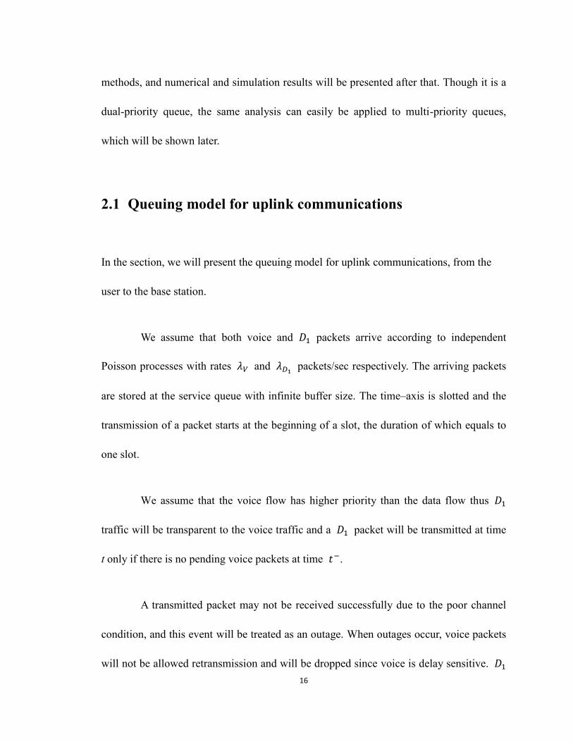
For a Poisson process with arrival rate , its exact energy function and

the asymptotic energy function when t goes to infinity are presented in [21],

and we notice is a Taylor approximation of for Poisson processes.

For Binomial process with success probability 1-q, its exact energy function

and the corresponding asymptotic energy function are presented in [21],

The asymptotic and the exact energy functions of Poisson and Binomial

processes are plotted in Fig. 2.1as a function of . We can see that the asymptotic results

are very close to the exact energy function for small values of . And for most stable

queues under heavy loading, the satisfy (2.4) is far less than 1. Thus we can conclude

that (2.9) is a good asymptotic result for the energy function of the departure process of

traffic when no voice traffic is involved.

24

(a) Energy function of Poisson process with arrival rate

(b) Energy function of Binomial process with success probability 1-q

Fig. 2.1 Comparison of energy function from central limit theorem for renewal processes and

the exact energy functions of Poisson and Binomial processes

25

2.2.2 Delay violation probability of traffic in the presence of voice

traffic

Next, we consider transmission of packets in the presence of voice, which

was described in the queuing model section. We let

,

denote the energy

functions of packet arrival and departure processes of traffic in the presence of voice.

We notice that

remains the same as since arrival processes are

independent. However,

differs from , since voice has priority over ,

traffic may only use the left over bandwidth from the voice traffic. Let

denote the number of data packets that may be served during a time interval [0, t) in the

presence of voice traffic, clearly, does not have the same distribution as .

So according to the definition of energy function in (2.3), we can conclude that

.

Unfortunately, we have not been able to determine thus cannot obtain

. It is another common bottleneck in a multi-priority queuing system to determine

the number of departures during a certain period for a low priority traffic, since it is very

complicated and most of the time there does not exist a closed form expression. As a

result of that, we propose the following approximation. Assuming

(2.10)

26

where is the number of voice packet arrivals during [0, t) and 1 corresponds to the

one slot for transmission of a voice packet. Since service of each voice packet takes one

slot, the above equation states that after voice arrival packets have all been served, during

[0, t), there is only a period of that can be used to serve packets. And that

period is exclusive for service for packets, just as in the sole case.

As we have shown in (2.9), can be approximated as a Gaussian random

variable with mean

, and variance

. So applying central limit theorem for renewal

processes again, we can say is also another Gaussian rv with mean

and variance

since goes to infinity as t goes to infinite. And recall the

definition of energy function in (2.3), we could have

assuming and are independent, we have

noticing that in the above expression, the argument in the is the probability

generating function (pgf) of and since voice arrival process is a Poisson process

with rate , then we have,

27

(2.11)

At this point, we have obtained the energy function of departure process of

traffic in the presence of voice in (2.11), by using an approximate method to obtain

in (2.10) and applying the asymptotic method to obtain

.

And substituting (2.5) and (2.11), the energy functions of arrival and departure

process of traffic in the presence of voice, into (2.4), we obtain the delay-bound

violation probability of traffic in the presence of voice,

(2.12)

where is the unique solution to the following set of equations,

The above equations cannot be solved analytically, but it is possible to solve them

numerically using Taylor expansion and that will be explained later on in the numerical

results section.

28

At this point, we have obtained the queuing delay violation probability based on

the queuing model described in section 2.1. Next, we are going to extend our analysis to a

tri-priority queue to demonstrate our analysis is feasible to any number of priority levels.

2.2.3 Extension of delay violation probability to multiple types of

traffic (more than two)

We have obtained the queuing delay violation probability for a dual-priority case

in (2.12) and (2.13). The analysis presented above can be easily extended to more than

two priorities by repeating the procedures in (2.10) and (2.11) to obtain the energy

function of the departure process whenever a new level is involved. For example,

assuming there is another data flow involving in the existing dual-priority queue with

the lowest priority. In this case, the queue is a tri-priority queue with voice having the

highest priority, traffic having the middle priority and traffic having the lowest

priority. Clearly, the delay for the traffic remains the same as before since traffic

is transparent to and voice. Now, if we want to obtain the queuing delay-bound

violation probability for the traffic, we can do the following work,

Applying the same procedure in (2.10) and (2.11), we then have,

(2.14)

29

from the definition in former analysis, we know is the number of voice packet

arrivals during [0, t), thus similarly we denote as the number of packet

arrivals during [0, t). For those arrival packets of data flow , assume that the

service time of each of them will take slots where i from 0 to , the pgf of

is and it is determined in (2.7). Also, we denote as the number of

packets that may be served during [0, t) if there is no other traffic involved, the

number of packets that may be served during a time interval [0, t) in the presence of

voice traffic and traffic.

Similar as in (2.10), equation (2.14) can be explained as before: if we subtract

the time period that is used for serving voice packets and packets, the remaining

period is then exclusive for the service for packets.

Let denotes the energy function of the arrival process of traffic.

Without loss of generality, we assume that packet arrival process is a Poisson process

with arrival rate packet/slot, so we have

just like (2.5).

And we also assume the saturated departure process of traffic is a renewal process

when no other traffic is involved in the system.

Defining as the energy function of departure process of traffic in

the sole case, and it can be defined as

. Since

we have assumed that the departure process of traffic is also a renewal process, using

30

the central limit theorem for renewal processes again we can obtain an asymptotic result

of , which is given by

just like in (2.9), while

is the

mean of the service time of a packet and the variance. Define

as

the energy function of the departure process of traffic in the tri-priority case, and it

can be expressed as

, Thus, according to (2.14) ,

we could have,

(2.15)

is the pgf of the Poisson packet arrival process of traffic with rate .

31

At this point, we have obtained the energy function of the departure process of

packet in the presence of voice and traffic. So we can determine the delay

violation probability for the traffic by substituting

and

into (2.4)

in the same way as (2.12) and (2.13).

From above, we can see our analysis is feasible for a tri-priority queuing system

with any arrival and departure processes, as long as those processes are renewal processes

which allow application of the central limit theorem for renewal processes to obtain the

asymptotic energy function of them.

Next, we summarize the procedure for application of the analysis to obtain the

delay violation probability of a traffic in a queuing system with any number of priority

levels,

1. Determine the energy function of the saturated departure process of the target traffic

with no other traffic involved using the central limit theorem for renewal processes.

2. Use the approximation method in (2.10) or (2.14) to obtain the number of departures of

the target traffic in the presence of other traffic by subtracting the time that is used for

higher level traffics.

3. Obtain the energy function of the departure process of the target traffic with all other

traffic involved by substituting the result from step 2.

4. Obtain the energy function of the arrival process of the target traffic using direct

32

analysis or asymptotic analysis from central limit theorem for renewal processes.

5. Substitute the energy function of the arrival/departure processes of the target traffic

into (2.4) to achieve the final queuing delay violation probability.

2.3 Numerical results

In this section, we present some numerical results regarding the analysis of the

dual-priority queue we have analyzed before.

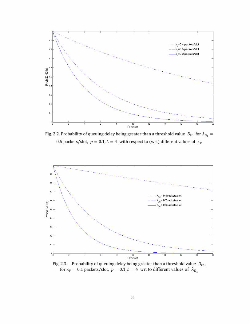
First, we present the delay violation probabilities as a function of the delay

threshold for the traffic in Fig.s 2.2, 2.3 and 2.4 with , , p and L as

parameters. From the figures, as expected, probability of delay violation increases as ,

, p or L increases. In Fig.s 2.4a, b the values of the outage probability is p=0.1 and 0.2

respectively and in Fig. 2.4a, the dashed curves corresponds to L = 4 and 8 which

overlaps with each other. This is because the retransmissions occur rarely since the

probability of outage has a low value, p = 0.1 and, as a result, the value of L does not

affect the delay much. However, in Fig. 2.4b it may be seen that the delay violation

probability increases sharply with L rising from 2 to 4. This is because of higher value of

the outage probability the retransmissions occur more frequently, which results in higher

delays.

33

Fig. 2.3. Probability of queuing delay being greater than a threshold value ,

wrt to different values of

Fig. 2.2. Probability of queuing delay being greater than a threshold value ,

with respect to (wrt) different values of

34

Fig. 2.5 presents packet loss probability as a function of the allowed maximum

number of transmissions of a packet, L, with probability outage p as a parameter. As may

be seen, packet loss probability decreases as L increases for fixed values of p. On the

(a)

(b)

Fig. 2.4. Probability of queuing delay being greater than a threshold value , for

wrt different transmission time L and

outage probability

35

other hand, packet loss probability increases as p increases for fixed values of L. We note

that results in this figure will also apply to voice for L=1.

Next, we discuss the tradeoffs between queuing delay, packet loss and

probability of outage. From Fig.s 2.4 and 2.5, we can reduce the packet loss probability

for traffics by increasing the number of transmission attempts, L, but, unfortunately, this

also increases the queuing delay. On the other hand, decrease in the probability of outage

will result in the reduction of both packet loss as well as the queuing delay. Also,

decrease in outage probability can also reduce the retransmission times thus save

bandwidth and energy. So a small outage probability is very crucial, in any wireless

networks. And that’s why we continue the work to obtain the optimum antenna layout

that achieves the minimum average outage probability of the DAS in Chapter 3.

Fig. 2.5. Probability of packet loss as a function of maximum number of transmissions of

a packet, L, wrt different outage probability

36

2.4 Simulation results

In this section we are going to present two simulation results for analysis of the

dual-priority queue in Figs 2.6 and 2.7. From the figures, we can see that simulation and

numerical computation matches perfectly well with each other. There are some slightly

differences between those two, that reason would be that randomness is hard to be

simulated appropriately in computer. Another reason might be using the central limite

theorem for renewal process to calculate the asymptotic energy function in (2.9), though

we have shown in Fig. 2.1 that for small it is a very good approximation, little

difference is still there. Also the approximate method used in equation (2.10) in

calculating the number of departures of a low priority traffic will introduce some error.

And in (2.11), since and are not independent form each other so

there exists another approximation there, which is represented below,

Despite all those approximations, comparisons of the results show that our

analysis still works perfectly for a multi-priority queuing system under heavy traffic load.

Further, the developed method can be applied to any generalized multi-priority queue

with any renewal arrive/departure processes, even whose energy functions are hard to

obtain.

37

Fig. 2.6. Simulation and numerical results of probability of queuing delay being greater than a

threshold value , for ,

Fig. 2.7. Simulation and numerical results of probability of queuing delay being greater than a

threshold value for

38

Chapter 3. Optimal placement of

antennas in DAS

As known from the previous chapter, the outage probability is an important QoS metric,

the reduction of it can reduce the queuing delay together with the packet loss probability,

and at the same time help increase the bandwidth and the power efficiencies. In this

chapter, we aim to obtain the optimal locations of distributed antennas in distributed

antenna system (DAS) such that the system’s average uplink outage probability is

minimized. Due to large mathematic difficulties, closed form expression of optimum

antenna layout could not be obtained, instead, numerical and simulation results are given.

3.1 System model

In the section, we will present the system model of distributed broadband wireless

communication system (BWC) which contains four subparts: network topology, channel

model, frequency reuse mechanism and uplink transmission scheme.

39

3.1.1 Network topology

First, we will describe the network topology. We will assume the distributed BWC system

having a cellular network architecture as shown in Fig. 3.1. In this architecture, cells form

clusters. Without loss of any generality, we will assume cluster size F to be 7. As shown

in Fig. 3.1, the cells in the clustered will be numbered as , i=0,…,F-1. And we will

refer cell as the target cell.

We show each cell as a circle rather than a hexagon since in reality, cells are

mostly in shape of circle, and hexagon is usually used as a theoretical approximation

model.

It is assumed that each cell contains a central processor and M distributed

antennas, which are placed at different geographical locations and each of these antennas

is connected to the central processor of its own cell through fiber lines. In Fig. 3.1 only

the antennas in the target cell have been shown to prevent crowding, however, each

of the other cells also contains M antennas which are deployed in the same manner as in

the target cell.

40

Fig. 3.1: Topology of the distributed BWC system which has a cellular network architecture

All the cells are assumed to have the same size with radius which has been

assigned an unitary value of . The locations of cell ’s center will be given by

, for i = 0,…, F-1, with respect to (wrt) a Cartesian coordinate system located

at the center of cell .

Stands for antenna.

Stands for the target user.

Stands for co-channel user.

Stands for the central processor.

41

In the target cell, locations of the M antennas wrt the cell center are denoted by

in polar coordinate system or in the Cartesian coordinate

system, for m=1,..., M and , with the assumption that all

the antennas have the same height , and the users are all at the ground level. This

assumption ensures that a user will always be in the far-field (will be introduced later in

section 3.1.2.1) of any antenna so we are avoiding the near-field antenna gain problem.

The relations between and can be expressed as,

As will be shown in the frequency reuse mechanism in section 3.1.3, for a

specific frequency channel, in each cell , i=0…F-1, we will assume only a single user

can use it and we will refer to that user as user i. The location of user i in polar

coordinates will be given by relative to the center of its cell. The location of

user i in Cartesian coordinates will be given by ( ) relative to the center of the target

cell , which may be expressed as,

Let denote the distance from mobile user i to the antennas in the

target cell, and it can be written as:

(3.1)

42

for i = 0, 1, …, , m=1,…M.

3.1.2 Channel model

We assume the uplink channel contains two types of fading, one is large-scale fading due

to path loss and the other is small-scale fading due to multipath propagation effects. The

combined model of these two fadings is then taken as the channel model.

3.1.2.1 Large-scale fading

The large scale fading refers to the drop of the received local average signal power as a

function of the distance between transmitter and receiver pair [14]. The large scale fading

is determined by the path-loss model below:

and are the received local average signal powers at receiver with distances

and away from the transmitter (in dB). In our case, we consider uplink

communications from user to antenna so receiver/transmitter pair refers to antenna/user.

43

Environment Path Loss Exponent,

Free Space 2

Urban area cellular radio 2.7 to 3.5

Shadowed urban cellular radio 3 to 5

In building line-of-sight 1.6 to 1.8

Obstructed in building 4 to 6

Obstructed in factories 2 to 3

Table 3.1: Path loss exponents for some typical environments [16]

is the far field distance and cannot be smaller than . “The far field

distance is related to largest linear dimension of the transmitter antenna aperture and the

carrier wavelength” [16]. Far field distance is determined because when the distance

between the transmitter and the receiver is less than the far field distance, the received

local average signal power does not follow the above model. Usually, the far field

distance is less than 1km for a large cell and 100m for microcells [15]

is the path loss exponent and is usually chosen between 2 to 6, depends on the

channel condition[16]. Table 3.1 presents the values of in some typical environments.

is a Gaussian rv with variance (in dB) representing shadowing, which is

not considered in this thesis due to its numerical complexity, just like in [11].

44

3.1.2.2 Small-scale fading

Figure 3.2: Small-scale fading superimposed on large-scale fading [15]

Small scale fading results from the multipath propagation effects in wireless

communications which may be caused by the little relative motion between the receiver

and transmitter pair, the presence of reflecting and obstructing objects in the channel or

the movements of them [14].

When there are large amount of multipath components and no line-of-sight (LoS)

component, the received signal power with small-scale fading has a Rayleigh distribution

[15]. This kind of small-scale fading model is also called Rayleigh fading model.

A good illustration of a combined large and small scale fading effect is presented

Receiver’s distance towards the transmitter

Sig

nal P

ow

er (DB

)

Small-scale fading

Large-scale fading

45

in Figure 3.2 [15]. And we will drive the expression for this channel model below.

Assuming that when a user is transmitting at distance 1 from an antenna, the

average received signal strength at the antenna is W. Then , the received signal

strength at the antenna m from any user i can be written as,

(3.2)

where is the path loss exponent represents for the large-scale fading. is an

identical independently distributed (i.i.d) normalized complex Gaussian random variable

which represents the Rayleigh fading model and the noise.

3.1.3 Frequency reuse mechanism

In this section, we will describe the frequency reuse model.

In a cellular network, usually there is a frequency reuse factor of for a

conventional cluster with F cells, just like the example in section 1.2.1. However, this

results in low spectrum efficiency. On the other hand, the increase of reuse factor results

in large co-channel interference. In this work, we assume aggressive frequency reuse

mechanism, with all the frequencies being available in every cell, or we can say that the

reuse factor is 1, as in [10]. The available spectrum will be divided into channels, each

46

user may be using a single channel at any time. We also assume that the system is

saturated so that at any time, all the channels will be busy.

In a cellular system, the major cause of an outage is the co-channel interference

from the nearest cells [12]. Let us consider the user in the target cell , which will be

referred as the target user. The co-channel interferences to the target user will come from

the single user using the same channel in each of the other cells in the cluster. In this

work, we treat the inter-cell interferences from the F-1 tier one neighboring users as the

only source of noise to a target user as well as the only cause of an outage, so in (3.2)

is assumed to be zero.

So the instantaneous SIR at the antenna m can be written as,

(3.3)

where is determined in (3.2) with has a zero value.

is the useful signal power from the target user 0. , the

co-channel interferences from other co-channel users, are taken as the only source of

noise and are assumed to be the only cause of outage as mentioned before. So in fact

is also the SNR at the antenna m.

47

3.1.4 Uplink transmission scheme

A user will broadcast its packet which will be received by the antennas in its cell,

the received signals will be locally decoded by those antennas and, the results will be

forwarded to the central processor through fiber lines, respectively. If at least one of the

antennas can decode the packet successfully, the central processor will receive the

transmitted packet correctly (local decoding in section 1.2.4). Then, the central processor

will take certain action towards processing the result, for example, it may send the result

to its affiliated antennas to perform a downlink action or it may pass the result to another

central processor to perform a handover.

On the other hand, if none of the antennas is able to decode the packet

successfully, then the central processor cannot receive the transmitted packet and this is

treated as an outage.

3.2 Outage probability of a single antenna with a given set of

user locations

In this section, we are going to present the analysis of , the outage

probability of the antenna with a given set of user locations , which is

defined as vector … . In section 3.2.1,

48

we will determine a general expression of . Then, in section 3.2.2 and 3.2.3

we will perform mathematic analysis to get a closed form expression through application

of Laplace transforms.

3.2.1 General expression of

First, we are going to derive a general expression of .

For a communication system, outage probability is generally given by [18]:

(3.4)

where R is the required transmission rate of user in bits/sec/Hz [11] and I denotes the

mutual information of the channel between the transmitter/receiver pair and I can be

expressed as [19],

(3.5)

where is the instantaneous SNR at the receiver side.

Substituting (3.5) into (3.4), the outage probability at antenna m for a specific

user locations set , can be written as:

(3.6)

49

Substituting (3.1), (3.2) and (3.3) into (3.6), we could have:

(3.7)

for i = 0, 1, …, , m=1,…M.

Let us define random variable (rv) as

and as

. We note that . Then we have,

(3.8)

Since is a normalized complex Gaussian rv, then has a Rayleigh

distribution and is an exponentially distributed rv with mean 1, thus is also

an exponentially distributed rv with mean

and variance

[20].

Defining K and as , and substituting

it into (3.8), we have . Thus (3.7) can be written as,

50

(3.9)

for i = 0, 1, …, , m=1,…M.

Equation (3.9) is the general expression of the outage probability of a single

antenna m with a given set of user locations , and it is equal to the probability of

rv being greater than zero.

3.2.2 The Laplace transform of the rv

Unfortunately, equation (3.9) does not give us an explicit closed expression for

, so in this section and section 3.2.3, we are going to apply Laplace

transform techniques to obtain a closed form expression of .

Let denote the probability density function (pdf) of the random variable

and its Laplace transform.

Define

as

, its Laplace transform and

the pdf of . From the definition of (3.9), we have,

51

thus,

(3.10)

where is the Laplace transform of the rv .

Since , we have

, and according to

Table 9.1 in [26], we have

where is the Laplace transform of the rv .

So equation (3.10) can be written as,

(3.11)

Also rv is the sum of independent exponentially distributed rvs

, so we could have,

where

since is an exponentially distributed rv with mean

and variance

.

52

Then substituting and into (3.11), we have,

=

(3.12)

The region of converge (ROC) of is

…

where represent the real part of s.

Let us define and as,

(3.13)

(3.14)

where , denote a distinct value and its frequency in the set

…

where with . We also

assume

since is the only value less than zero and we have

.

Substituting (3.13) and (3.14) into (3.12), then we have

53

(3.15)

At this point, we have obtained the Laplace transform of .

3.2.3 The inverse transform of and

Next, we are going to invert to obtain and the closed form expression of

.

Using partial fraction expansion in that we had in (3.14), we could have

(3.16)

where

, pleases notice that j in

is the

superscript, not for power.

Then taking the inverse transform of in (3.16) and then of (3.15), we

obtain , the pdf of the rv ,

(3.17)

where

the reason that there exists a unique term in (3.17) is because that

54

in (3.14) and (3.16), is the only one less than zero, so according to the inverse

Laplace transform Table 9.2 in [26], we obtain this unique term with a while

other terms end up with .

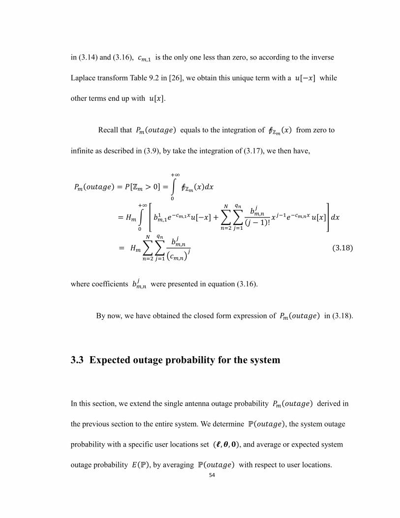
Recall that equals to the integration of from zero to

infinite as described in (3.9), by take the integration of (3.17), we then have,

where coefficients

were presented in equation (3.16).

By now, we have obtained the closed form expression of in (3.18).

3.3 Expected outage probability for the system

In this section, we extend the single antenna outage probability derived in

the previous section to the entire system. We determine , the system outage

probability with a specific user locations set , and average or expected system

outage probability , by averaging with respect to user locations.

55

Since outage of the antennas are assumed to be independent of each other, the

total outage probability of a cell with M antennas with a specific set of is given

by,

(3.19)

Next, unconditioning the above result wrt the user locations vector , we

can obtain the average or expected outage probability for the system ergodically,

…

…

…

where are the marginal pdfs of the coordinates of user i, and

respectively, denotes the expected value wrt the locations of the users. And since

we are assuming that users are uniformly distributed in a cell, we have the cumulative

distribution function (cdf) for rv as

, and substituting r=1 into it,

we have,

(3.21)

Substituting (3.21) into (3.20), we have

…

…

…

56

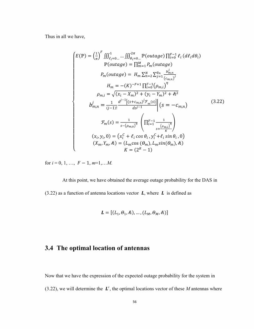
Thus in all we have,

…

…

…

(3.22)

for i = 0, 1, …, , m=1,…M.

At this point, we have obtained the average outage probability for the DAS in

(3.22) as a function of antenna locations vector , where is defined as

…

3.4 The optimal location of antennas

Now that we have the expression of the expected outage probability for the system in

(3.22), we will determine the , the optimal locations vector of these M antennas where

57

…

. The antenna locations vector that minimize the

expected outage probability of the system will be defined as optimal.

We can determine the minimum of by setting the gradient of in

(3.22) to a zero vector: , wrt to the antennas location vector

(3.23)

Among all the vectors that satisfy the above equation set, we choose one with

the minimum value of to be the optimum locations of those M antennas, .

We can also use Leibniz differentiation rule to change the order of derivatives

and integrations of equation (3.23), and obtain (3.24)

(3.24)

Again among all the vectors that satisfy the above equation set, we choose one

with the minimum value of to be .

Unfortunately, due to mathematic complexity, we cannot get a closed form for

the optimal locations of antennas with either approach.

Next, we consider the following simplification. Since all the cells are identical in

every aspect, we expect the locations of antennas to be symmetric in each cell. This

58

means that the antennas in a cell will be at the same distance from the cell center and the

space between two neighboring antennas will be the same. Thus, it is expected that the

antennas will be on a circle centered at the cell center, just as in [6]. This antenna layout

is shown in Fig. 3.2, with four antennas in the target cell in a symmetric placement.

Fig. 3.3: Topology of distributed BWC system with antennas symmetrically deployed on a circle

Stands for antenna.

Stands for the target user.

Stands for co-channel user.

Stands for the central processor

59

However, even with this assumption, we could not obtain a closed form due to

large mathematic difficulties in performing integrations and derivatives. As a result, we

have no choice but to obtain results through numerical calculations and simulations.

3.5 Numerical results

Theoretically, by turning the infinite integrations with respect to the users’ locations

in equation (3.22) into finite numerical accumulations, with the assumption of a

circular symmetric antenna layout, we may obtain with a certain antenna locations

vector . And after we apply the above procedure for every possible antenna locations,

the vector which achieves the minimum value of is then our optimum antenna

layout, . Explicitly, the density of possible locations of users and candidate antenna

will decide the accuracy of the numerical result.

However, the computation complexity limits us from obtaining accurate

numerical results which may require months of computer computations. So below we are

going to present a Robbins-Monro iterative algorithm from stochastic approximation

theory to obtain the optimum antenna layout.

Before we present the Robbins-Monro procedure, we will first give the system

parameters for numerical computations. We assume a circular symmetric antenna layout

60

with four antennas in a cell, M=4, see Fig. 3.3. Antenna’s height is assumed to have

value of , R is assumed a value of 1 bits/sec/Hz, is assumed a value of 4, which is

a typical path loss exponent in wireless communication model as in [6]. We will carry the

above assumptions and parameters to perform the Robbins-Monro iterative algorithm.

Also we define the first antenna with the coordinate

3.5.1 Brief introduction of Robbins-Monro algorithm

In this section, we are going to give a brief introduction of Robbins-Monro algorithm

from stochastic approximation theory.

Robbins-Monro algorithm is an iterative stochastic approximation algorithm. It

applies an iterative estimation procedure via noisy observations to find the values or

extremes of functions which cannot be obtained directly through regular mathematical

analysis [29].

For example, if we have a function that cannot be observed directly or

having a very complicated expression, and we want to obtain the root of the equation

y, where y is a constant value, we can apply the following procedure iteratively to

obtain ,

61

where … is a sequence of positive step sizes and the expected value of function

equals to , which can be expressed as . Or we can say that

is a noisy observation or an unbiased estimator of [10]. And Robbins and

Monro proved that converges to as n increases, provided that [29],

1. is uniformly bounded

2. is non decreasing

3. exists and is positive

4. satisfies the following requirements: and

Polyak and Juditsky proposed an improved version of Robbins-Monro algorithm

to accelerate the outcome of the above algorithm [30],

and converges to given that the constraints 1 to 3 in the above are satisfied and

sequence satisfy and

.

represents that grows much slower than does,

formally, it means that for any positive constant there exists a constant such that [31]

, for all

62

An example of a such sequence of step size may be , where 0<a<1,

and A is a positive value [30].

3.5.2 Application of Robbins-Monro algorithm in obtaining optimum

antenna layout

Using the same procedure described in section 3.5.1, we treat

as

and

as [10]. And from (3.24), which is presented again below, we

can tell is an unbiased estimator of and we have .

Next, we are going to perform the following Robbins-Monro procedure to obtain

the optimum antenna layout similar as in [10],

a. Initial an antennas location vector and set n=1

b. Randomly generate a users location vector according to their uniform

distributions in a cell.

c. Upgrade the optimum locations by applying the equation below

d. Let n=n+1 and iteratively run steps b, c, d until converges, where

63

. And converges to the optimum antenna location vector .

In our implementation of Robbins-Monro algorithm, we choose the sequence of

positive as , which satisfies the Polyak and Juditsky constraints

described at the end of section 3.5.1.

The outcome is shown below in Table 3.2. Since the antennas are symmetrically

located on the circle centered at the cell center, we only consider the first antenna’s

location with the coordinate , with .The locations of the

other three antennas can be easily obtained. Since from results, the values of are

all very close to zero, we are not showing them in the table. So in the following table we

only show the results of , which is also the radius of the antennas circle.

From the table below, we can tell that the converges to 0.58. So the

optimum location of the first antenna is , and the other three antennas are

at locations

, ,

respectively. This

optimum antenna layout achieves the minimum average uplink outage probability of the

distributed antenna system with the value of 0.0087.

64

n

ddddddddddddddddddddddd

1 0.00 31 0.54 61 0.58

2 0.90 32 0.54 62 0.58

3 0.63 33 0.54 63 0.58

4 0.54 34 0.54 64 0.58

5 0.50 35 0.55 65 0.58

6 0.47 36 0.55 66 0.58

7 0.45 37 0.55 67 0.58

8 0.46 38 0.55 68 0.58

9 0.48 39 0.55 69 0.59

10 0.49 40 0.55 70 0.59

11 0.50 41 0.55 71 0.59

12 0.50 42 0.56 72 0.59

13 0.50 43 0.56 73 0.59

14 0.51 44 0.56 74 0.59

15 0.51 45 0.56 75 0.59

16 0.51 46 0.56 76 0.58

17 0.51 47 0.56 77 0.58

18 0.51 48 0.56 78 0.58

19 0.52 49 0.57 79 0.58

20 0.52 50 0.57 80 0.58

21 0.52 51 0.57 81 0.58

22 0.52 52 0.57 82 0.58

23 0.53 53 0.57 83 0.58

24 0.53 54 0.57 84 0.58

25 0.53 55 0.57 85 0.58

26 0.54 56 0.57 86 0.58

27 0.54 57 0.58 87 0.58

28 0.54 58 0.58 88 0.58

29 0.54 59 0.58

30 0.54 60 0.58

Table 3.2 Robbins-Monro outcome of the optimum location of the first antenna with four

antennas in a cell

65

3.6 Simulation results

We are going to show our simulation results in this section. In section 3.6.1, we will

describe our simulation procedures. And the simulation result for a circular symmetric

antenna layout is shown in section 3.6.2 with M=4, and from it we can see that numerical

and simulation results are close. We will also take a look at the worst case in section 3.6.3.

The worst case represents the situation that the co-channel interferences are the most

severe, which means that the neighboring users are at the closet locations towards the

target cell.

Section 3.6.2 and 3.6.3 are both based on a 4 antennas assumption. We will show

the same kind of results for 1,5 antennas in section 3.6.4. And a summary will be given

after that in section 3.6.5.

3.6.1 Simulation procedures

The procedure of the Matlab simulation is briefly introduced below.

We apply Monte-Carlo algorithm in the simulation following equation (3.7) and

(3.19) which will be rewritten below,

66

(3.7)

(3.19)

We assume the first antenna has the following possibilities locations, is

chosen from (0, 0.05, 0.1,… ,1) and is chosen from (0,

,

,… ,

). The

remaining M-1 antennas are placed on the circle collocated at the cell center with the

radius that equals to the distance of the first antenna and the arc length between the

neighboring antennas are equal with the value of

. Once the location of the first

antenna is chosen, the whole topology of DAS is fixed. So there are

candidate antenna locations vectors .

For each , I will randomly generating 10000 user locations vector ,

according to users’ distribution. And for each of these user locations vector, I will

calculate the distance and generate exponential rvs vector 1000 times, where

… using Matlab times. Then using (3.7), for each , I can

count the number of events that satisfies

, where

67

event means an outage occurs at antenna m. Dividing the number of

outage events by 1000, then that’s our with one specific user locations

vector. Next, following equation (3.19) we could obtain . After that, I will

uncondition the user locations by averaging over those 10000 user locations vector. In

this way I can obtain the for one candidate antenna locations vector . And after

repeating the above steps and obtaining 188 values of , I will choose the one with

minimum value and the corresponding antenna locations vector will be our optimum

antenna layout .

Comparing to numerical computation, simulation is a more feasible method

since it’s much faster. Optimum antenna layout can be achieved in just several hours

using simulation.

For the simulation, antenna’s height is assumed a value of 0.05, R is assumed

a value of 1 bits/sec/Hz, is assumed a value of 4, and M=4. These parameters are

chosen the same as in the numerical computation.

3.6.2 Optimum antenna layout for M=4

In this section, we will show the simulation result of optimum antenna layout for circular

symmetric antenna layout with M=4.

68

From simulation results, we find that the optimal radius of the antenna circle is

0.55, which results in the minimum expected value of outage probability of

. Comparing to the case that all the antennas are at the center, the optimal location

provides almost 40% improvements in system’s average outage probability. Fig. 3.4

shows the for 4 antennas as a function of the first antenna’s location .

Different curves representing different angle . We can see the value of has minor

impact on and that’s why we only show the optimum radius. Also, we can tell that

the optimum antenna layouts obtained through simulation and numerical computations

are similar. (in numerical results, the minimum average uplink outage probability of the

DAS has the value of 0.0087 when the radius of antennas circle is 0.58.)

Fig. 3.4: Simulation result for system’s average outage probability for 4 antennas as a function of

the first antenna’s location.

69

3.6.3 Worst Case for M=4

In this section, we are going to present the simulation result for the worst case in Fig 3.5.

This is not for minimizing system’s average outage probability , but for minimizing

when the co-channel interferences are the most severe, which means that the

neighboring users are at the closet locations towards the target cell.

Fig. 3.5: Simulation result for outage probability for 4 antennas as a function of the first antenna’s

location in the worst case.

From Fig. 3.5, we can see that when antennas’ distances to the center are 0.5, the

outage probability is minimized at 0.2987. This is 33 times worse than the optimized

average outage probability of the system.

70

3.6.4 1, 5 antennas

In this section, we are going to present the optimum results for the average case together

with the worst case for M=1, 5.

71

3.6.4.1 M=1

A. For the system’ average outage probability

Fig. 3.6 a: Simulation result for system’s average outage probability for 1 antenna as a

function of the first antenna’s location

B. For the worst case outage probability

Fig. 3.6 b: Simulation result for outage probability for 1antenna as a function of the first

antenna’s location in the worst case.

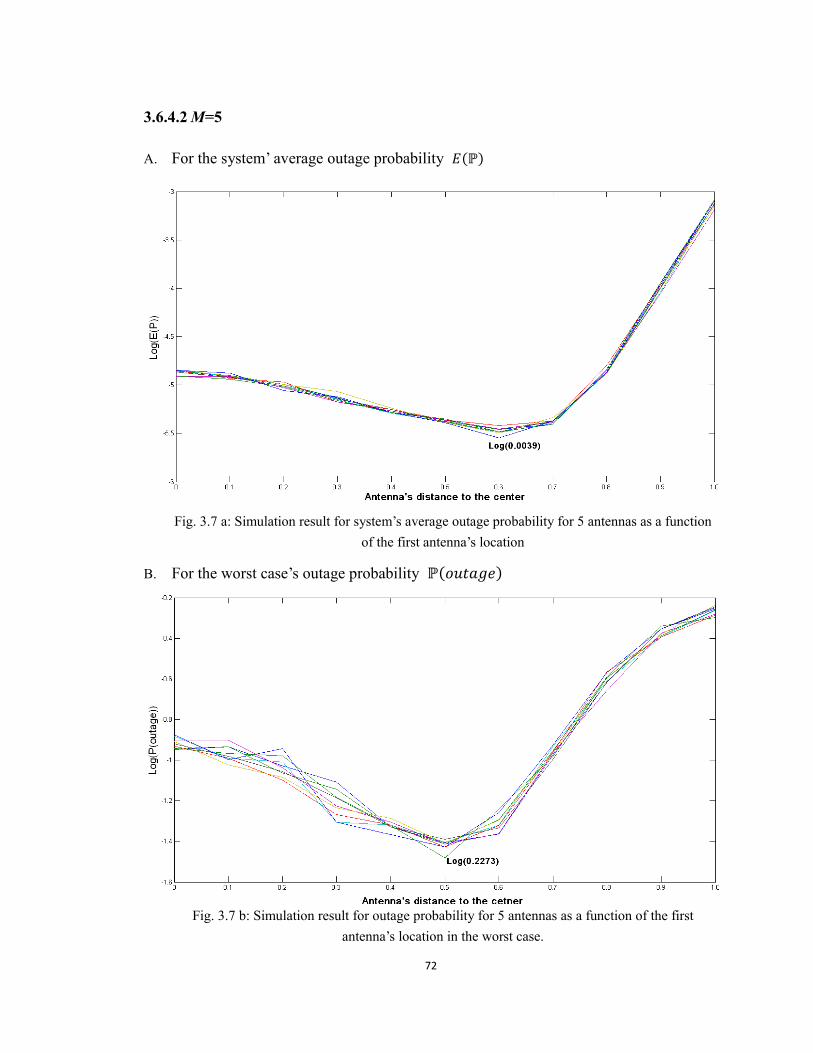
72

3.6.4.2 M=5

A. For the system’ average outage probability

Fig. 3.7 a: Simulation result for system’s average outage probability for 5 antennas as a function

of the first antenna’s location

B. For the worst case’s outage probability

Fig. 3.7 b: Simulation result for outage probability for 5 antennas as a function of the first

antenna’s location in the worst case.

73

3.6.5 Summaries

In this section, we are going to give summaries of the simulation results for different

value of M .

A. For minimizing system’ average outage probability

1 antenna 2 antennas 3 antennas 4 antennas 5 antennas

Average outage

probability

0.1864 0.0633 0.0233 0.0090 0.0039

Antenna’s optimum

distance to the center

0 0.2 0.5 0.55 0.6

Improvements of deploying

one more antenna

0 0.1231 0.04 0.014 0.0054

Improvements in

percentage

0 66% 63% 61% 57%

Table 3.3: Optimum radius of antenna circle for minimizing

B. For minimizing in the worst case

1 antenna 2 antennas 3 antennas 4 antennas 5 antennas

in the

worst case

0.6205 0.4841 0.3629 0.2987 0.2273

Antenna’s optimum

distance to the center

0 0.3 0.5 0.5 0.5

Improvements of deploying

one more antenna

0 0.1364 0.1312 0.0542 0.0714

Improvements in

percentage

0 22% 23% 15% 24%

Table 3.4: Optimum radius of antenna circle for minimizing in the worst case

From Table 3.3, we can see that for , a new antenna will bring improve 62%

in performance. And as the amount of antenna increases, the radius of antenna circle

74

asymptotically reaches 0.6. We did not present the angle of the antenna’s location in the

above table since figures above show that angles have minor influence on the optimum

locations of antennas.

From Table 3.4, we can see that for minimizing in the worst case, a

new antenna will improve about 20% in performance. From Figs. 3.5 to 3.7, we can see

though the angles do influence the outage probability , as M rises, the impact

of it is reducing, and when M=5, the influence is very little, as shown in Fig. 3.7. So no

information of angle is presented here either.

The above two tables are summarizes of the simulation results. The results are

based on our earlier assumptions that the antennas are symmetrically distributed on a

circle centered at the center of the cell, and radius of each cell has the unitary value of 1.

The antenna’s height has value of 0.05, the path-loss exponent , and the

required transmission rate R=1 bit/Hz/Sec. Explicitly, a higher R will result in higher

outage probability and vice the verse.

At this point, we have obtained the optimum antenna layout through numerical

computations and simulations. We have tried to obtain the optimum placements of

antennas for minimizing system’s average uplink outage probability by making several

reasonable assumptions for simplification: 1. There is no source of noise other than

co-channel interferences; 2. The antennas are symmetrically distributed on a circle

75

centered at the center of the cell.

From the numerical and simulation results, we can tell that the optimum antenna

layout is depending on the amount of antennas, and the optimal locations of the antennas

are not at the cell center except for the 1 antenna case. Also, radius of antennas circle

dominates the outage probability, while the corresponding angles influence little.

Furthermore, every time one more antenna being deployed, it can improve 62% in the

system’s average outage probability , and about 20% improvements to

in the worst case whereas the antenna circle expands as the amount of antennas increases

in both average and worst case.

Also, we notice that in this chapter are relatively smaller than the outage

probability we have been using in studying the queuing delay violation probability in

Chapter 2 with the value , the reason for that is in Chapter 3 we have chosen R

the required transmission rate of a user, to be a small value of R=1 bit/Hz/Sec. However,

when R increases, will increase for sure. For example, when R=2 bit/Hz/Sec, the

minimum value of system’s outage probability achieves 0.067 when the radius of

antennas circle has the value of 0.5. This is obtained through simulation.

76

Chapter 4. Conclusion and future work

Presently, distributed broadband wireless communication (BWC) system is a very

promising wireless technology due to its low cost and high performance. It contains a

distributed antenna system (DAS) connected to a base station with optical fiber. This

thesis determines the queuing delay violation probability for a multi-priority queue under

heavy traffic load as a function of the outage probability of the DAS. The relation

between these two QoS metrics is presented. And we have also studied the optimum

antenna layout that minimizes the antenna outage probability.

In the queuing delay violation probability analysis, an asymptotic method is

adopted for calculating the energy functions using the central limit theorem for renewal

processes, and an analytical approximation is given to calculate the number of departures

of a low priority traffic in the presence of high priority traffics in a certain duration. With

the above two steps, we could obtain the queuing delay violation probability for a general

multi-priority queue with any number of priority levels and arbitrary renewal

arrival/departure process while former works are mostly focusing on single priority queue

with constant arrival/departure rate. Numerical results show that the reduction in outage

77

probability will not only improve the queuing delay but also reduce the packet loss

probability; it will also improve the bandwidth and energy efficiencies. Simulation results

have been also presented to show accuracy of our analysis.

Since outage probability is a crucial factor in the QoS and performance of DAS,

we have investigated the optimum distributed antenna layout that results in the minimum

average uplink outage probability. The studied model includes path-loss and Rayleigh

fadings, and inter-cell interferences are properly taken into account in our cellular

topology. The exact distribution of the system’s outage probability with a given set of

user locations has been determined and this achievement appears to be the first in the

literature. Unfortunately, the closed form expression of the optimum antenna layout could

not be obtained due to huge mathematic complexity, even with the simplification that

antennas will be symmetrically located on a circle centered at the cell center. Thus, we

turn obtain the numerical results of the optimum antenna layout using Robbins-Monro

algorithm from stochastic approximation. The results show that for a cell with 4 antennas,

the optimum radius of the antenna circle is 0.58 which achieves the minimum outage

probability of 0.0087 for R=1 bits/sec/Hz. Simulation results show that deployment of

one more antenna can bring almost 62% improvement in the system’ average outage

probability , and about 20% improvement in the system’s outage probability

in the worst case whereas the antennas circle expands as the amount of

antennas increases in both average and worst case.

78

Our analysis on the queuing delay violation probability and the optimum antenna

layout in DAS will be useful in designing distributed BWC systems and the results are

very easy to use. What’s more, it should be noted that the analysis of queuing delay

violation probability is not just limited to the distributed BWC systems, in fact, it is quite

general and it applies to the delay attribute of a multi-priority queue with renewal arrival

and departure processes in any kind of communication system.

The following possible future works is envisioned,

1. Derivation of a closed form of the optimum antenna layout, though huge mathematic

complexities are involved.

2. Extending the optimum antenna layout study by including power constraints on each

user since power consumption is a very important issue, examples might be [9] and

[10].

3. Try the analysis of optimum antenna layout based on the combination of DAS and

CAS. This combined system model might provide a smooth transition from CAS to

the DAS by using existing infrastructures.

4. Verify the discovery from simulation results in [10] that shadowing or multi-path

Raleigh fading has no effect on the optimal location of antennas in optimizing

79

system’s capacity. If this conclusion is true, it will help reduce the complexity a lot in

dealing with similar problems.

5. While the required transmission rate R of users are different which is exactly what

happens in the real world, the optimum antenna layout in minimizing the average

uplink outage probability of the system should be a function of the distribution of R.

And the work on this problem may have to be depend on either solving problem 1 or

4.

80

References

[1] Mohr, W. ; Monserrat, J.F. ; Osseiran, A. ; Werner, M. “IMT-ADVANCED AND

NEXT-GENERATION MOBILE NETWORKS [Guest Editorial]” in Communications

Magazine, IEEE Volume : 49 , Issue:2 page(s): 82 – 83, February 2011

[2] Wang, Jiangzhou; Adachi, F.; Gameiro, A.; Gomes, N.J.; Kitayama, K-I.; Monteiro, P.;

Sawahashi, M.; Xia, Xiang-Gen “Guest Editorial: Distributed Broadband Wireless

Communications” in Selected Areas in Communications, IEEE Journal on, Volume: 29 ,

Issue: 6 Page(s): 1121 – 1122, 2011

[3] Jungwon Lee; Toumpakaris, D.; Wei Yu “Interference Mitigation via joint detection”

in Selected Areas in Communications, IEEE Journal on, Volume: 29 , Issue: 6 Page(s):

1172 – 1184, 2011

[4] Clark, M.V.; Willis, T.M., III; Greenstein, L.J.; Rustako, A.J., Jr.; Erceg, V.; Roman,

R.S. “Distributed Versus Centralized Antenna Arrays in Broadband Wireless Networks”

in VTC 2001 Spring. IEEE VTS 53rd , Volume: 1 Page(s): 33 – 37, 2001

81

[5] Wei Feng; Xibin Xu; Shidong Zhou; Jing Wang; Minghua Xia “Sum Rate

Characterization of Distributed Antenna Systems With Circular Antenna Layout” in

Vehicular Technology Conference, 2009. VTC Spring 2009. IEEE 69th , Page(s): 1 – 5,

2009

[6] Jiansong Gan; Yunzhou Li; Shidong Zhou; Jing Wang “On Sum Rate of Multi-User

Distributed Antenna System With Circular Antenna Layout” in Vehicular Technology

Conference, 2007. VTC-2007 Fall. 2007 IEEE 66th , Page(s): 596 – 600, 2007

[7] Wei Feng; Yunzhou Li; Jiansong Gan; Shidong Zhou; Jing Wang; Minghua Xia “On

the Size of Antenna Cluster in Multi-User DAS” in Communications and Networking in

China, 2008. ChinaCom 2008. Third International Conference on , Page(s): 1101 – 1105,

2008

[8] Hairuo Zhuang; Lin Dai; Liang Xiao; Yan Yao “Spectral efficiency of distributed

antenna system with random antenna layout” in Electronics Letters, Volume: 39 , Issue:

6 ,Page(s): 495 – 496, 2003

[9] Lin Dai “A Comparative Study on Uplink Sum Capacity with Co-Located and

Distributed Antennas” in Selected Areas in Communications, IEEE Journal on, Volume:

29 , Issue: 6 ,Page(s): 1200 – 1213, 2011

82

[10] Firouzabadi, S.; Goldsmith, A.” Optimal Placement of Distributed Antennas in

Cellular Systems” in Signal Processing Advances in Wireless Communications (SPAWC),

2011 IEEE 12th International Workshop on, Page(s): 461 – 465, 2011

[11]Zennaro, D.; Tomasin, S.; Vangelista, L. “Base Station Selection in Uplink Macro

Diversity Cellular Systems with Hybrid ARQ” in Selected Areas in Communications,

IEEE Journal on, Volume: 29 , Issue: 6 Page(s): 1249 – 1259, 2011

[12]Linnartz, J.-P.M.G. “Exact Analysis of the Outage Probability in Multiple-User

Mobile Radios” in Communications, IEEE Transactions on , Volume: 40 , Issue: 1

Page(s): 20 – 23, 1992

[13] Qinghe Du; Xi Zhang “QoS-Aware Base-Station Selections for Distributed MIMO

Links in Broadband Wireless Networks” in Selected Areas in Communications, IEEE

Journal on Volume: 29 , Issue: 6 Page(s): 1123 – 1138, 2011

[14]Alighanbari, A.; Sarris, C.D. “High Order S-MRTD Time-Domain Modeling of

Fading Characteristics of Wireless Channels” in Antennas and Propagation Society

International Symposium 2006, IEEE Page(s): 2165 – 2168, 2006

[15] Bernard Sklar “Digital Communications, Fundamentals and Applications,2nd

edition.” Chapter 15 Prentice Hall PTR , January 11, 2001

83

[16] Theodore S. Rappaport “Wireless Communication Principles and Practice. Chapter4”

Prentice Hall PTR, 1996

[17] Youssef, N.; Kawabata, T. “On the probability density functions of outage and

inter-outage durations of the capacity of Rayleigh fading channels” in Wireless

Communications, IEEE Transactions on , Volume: 8 , Issue: 2 Page(s): 529 – 534 ,

2009

[18]Yi Zhao; Adve, R.; Teng Joon Lim “Outage Probability at Arbitrary SNR with

Cooperative Diversity Networks” Communications Letters, IEEE , Volume: 9 , Issue: 8

Page(s): 700 – 702, 2005

[19] T.M. Cover and J.A.Thomas “Element of Information Theory”, John Wiley,1991

[20] Alberto Leon-Garcia “Probability, Statistics and Random Process for Electrical

Engineering 3rd edition”, Pearson Prentice Hall, 2008

[21]Peter Rabinovitch& Danny De Vleeschauwer “What is EffectiveBandwidth”

http://www3.sympatico.ca/peter.rabinovitch/eb.pdf

[22] Chen-Shang Chang; Thomas, J.A. “Effective Bandwidth in High-speed Digital

Networks” in Selected Areas in Communications, IEEE Journal on , Volume: 13 , Issue: 6

Page(s): 1091 – 1100, 1995

84

[23] Dapeng Wu; Negi, R. “Effective Capacity---A Wireless Link Model for Support of

Quality of Service” in Wireless Communications, IEEE Transactions on , Volume: 2 ,

Issue: 4 Page(s): 630 – 643 , 2003

[24] Xinzheng Wang; Pengcheng Zhu; Ming Chen “Antenna Location Design for

Generalized Distributed Antenna Systems” in IEEE COMMUNICATIONS LETTERS,

VOL. 13, NO. 5, MAY 2009

[25] Yunzhi Qian; Ming Chen; Xinzheng Wang; Pengcheng Zhu “Antenna Location

Design for Distributed Antenna Systems with Selective Transmission” in Wireless

Communications & Signal Processing, 2009. WCSP 2009. International Conference on,

2009

[26] Alan V.Oppenheim, Alan S.Willsky with S.Hamid Nawab “Signals and Systems”

second edition, Prentice Hall

[27] International Telecommunication Union “ITU-R M.1645: Framework and overall

objectives of the future development of IMT-2000 and systems beyond IMT-2000”

[28] William Feller “An Introduction to Probability Theory and Its Applications, Volume

2”, Chapter Ⅺ,John Wiley & Sons, Inc.

85

[29] Harold J.Kushner and Dean S.Clark “Stochastic Approximation Methods for

Constrained and Unconstrained Systems”, Chapter 1, Spinger-Verlag, New York,

Heidelberg, Berlin

[30] B. T. Polyak and A. B. Juditsky “Acceleration of Stochastic Approximation by

Averaging” SIAM J. CONTROL AND OPTIMIZATION Vol. 30, No. 4, pp. 838-855, July

1992

[31] Ronald Graham, Donald Knuth, and Oren Patashnik “Concrete mathematics (2

ed.)”. p. 446, Addison-Wesley, 1994