qps - vital imagesvitreawebeu.vitalimages.com/vital/help/en/pdf/qps_ref.pdf · qps (quantitative...
TRANSCRIPT

Cedars-Sinai Medical Center Department of Medicine
Artificial Intelligence in Medicine Program
This document and the technology described herein are the property of Cedars-Sinai Medical Center and shall not be reproduced, distributed or used without permission from an authorized company official. This
is an unpublished work subject to Trade Secret and copyright protection.
Copyright © 2011 Cedars-Sinai Medical Center
QPS
Quantitative Perfusion SPECT
Reference Manual
Version 2012.1: October 2011
Options: ARG, QPET, PlusPack20, Fusion, Coronary Tree
2
Warranty and Copyright Statement
Cedars-Sinai Medical Center has taken care to ensure the accuracy of this document. However, Cedars-Sinai Medical Center assumes no liability for errors or omissions and reserves the right to make changes without further notice to any products herein to improve reliability, function, or design. Cedars-Sinai Medical Center provides this guide without warranty of any kind, either implied or expressed, including, but not limited to, the implied warranties of merchantability and fitness for a particular purpose. Cedars-Sinai Medical Center may make improvements or changes in the product(s) and/or program(s) described in this manual at any time.
This document contains proprietary information which is protected by copyright. All rights are reserved. No part of this manual may be photocopied, reproduced, or translated to another language without written permission from Cedars-Sinai Medical Center.
Cedars-Sinai Medical Center reserves the right to revise this publication and to make changes in content from time to time without obligation on the part of Cedars-Sinai Medical Center to provide notification of such revision or change.
Copyright © 2011 Cedars-Sinai Medical Center Artificial Intelligence in Medicine (AIM) Program 8700 Beverly Blvd., CA, 90048, USA
Property of Cedars-Sinai Medical Center
Disclaimer
Neither Cedars-Sinai Medical Center, its parent, nor any of its worldwide affiliates shall be liable or obligated in any manner in respect of bodily injury and/or property damage from the use of the system/software if such is not in strict compliance with instructions and safety precautions contained in the relevant operating manuals and in all supplements thereto, in all product labels, and according to all terms of warranty and sale of the system, or if any change not authorized by Cedars-Sinai Medical Center is made to the software operating the system.
Trademarks
ADAC®, AutoQUANT®, AutoSPECT®, AutoSPECT®Plus, CardioMD®, CPET®, ENsphere®, Forte™, GEMINI™, GENESYS®, InStill®, JETSphere™, JETStream®, MCD/AC™, Midas™, Pegasys™, Precedence™, SKYLight®, Vantage™, and Vertex™ are trademarks or registered trademarks of Philips Medical Systems.
Adobe, the Adobe logo, Acrobat, the Acrobat logo, and PostScript are trademarks of Adobe Systems Incorporated or its subsidiaries and may be registered in certain jurisdictions.
UNIX® is a registered trademark of The Open Group.
Linux is a trademark of Linus Torvalds and may be registered in certain jurisdictions.
Microsoft and Windows are either registered trademarks or trademarks of Microsoft Corporation in the United States and/or other countries.
Other brand or product names are trademarks or registered trademarks of their respective holders.

3
User Assistance Information For assistance please visit our website or contact us via e-mail:
[Website] www.csaim.com
[E-mail] [email protected]

4
Table of Contents 1 Introduction ................................................................................................................................... 8
2 Interface ........................................................................................................................................ 10
2.1 Main Controls ....................................................................................................................... 10
3 Viewing Images ............................................................................................................................. 11
3.1 Viewing Slices........................................................................................................................ 12
3.2 Viewing Surfaces ................................................................................................................... 12
3.3 Viewing Polar Maps .............................................................................................................. 13
3.4 Study Selector ....................................................................................................................... 13
3.5 Dataset Selector .................................................................................................................... 13
3.6 Dataset Editor ....................................................................................................................... 14
3.7 Color Scale Control ............................................................................................................... 15
3.8 Score Box ............................................................................................................................... 16
3.9 Info Box ................................................................................................................................. 17
4 Pages.............................................................................................................................................. 19
4.1 Raw Page .............................................................................................................................. 20
4.2 Slice Page ............................................................................................................................... 21
4.3 Surface Page .......................................................................................................................... 21
4.4 Splash Page ........................................................................................................................... 22
4.5 Views Page ............................................................................................................................ 23
4.6 Results Page.......................................................................................................................... 24
4.7 More Page ............................................................................................................................. 25
5 Manual Mode ............................................................................................................................... 25
5.1 Transverse Manual Mode .................................................................................................... 26
6 Change Page ................................................................................................................................. 27
6.1 Requirements ....................................................................................................................... 28
6.2 Implementation ................................................................................................................... 28
6.3 Reviewing Results on the Change page............................................................................... 29
Assessing Change results ............................................................................................................. 29
6.4 Controls ................................................................................................................................ 29
6.5 Roving Window ................................................................................................................... 30
7 QPC Page ...................................................................................................................................... 31
5
7.1 Feature Requirements .......................................................................................................... 32
7.2 Implementation ................................................................................................................... 33
7.3 Reviewing Results on the QPC page ................................................................................... 33
Assessing Slices, Polar Maps and Surfaces ................................................................................. 34
7.4 Page Controls ....................................................................................................................... 34
8 Fusion Page .................................................................................................................................. 35
8.1 Feature Requirements .......................................................................................................... 35
8.2 Implementation ................................................................................................................... 35
8.3 Reviewing Images on the Fusion page ................................................................................ 36
8.4 Controls ................................................................................................................................ 36
8.5 Mouse Controls .................................................................................................................... 36
8.6 Keyboard Controls ............................................................................................................... 37
8.7 Roving Window ................................................................................................................... 37
9 Coronary CTA Vessels Display .................................................................................................... 38
10 Kinetic Page - Coronary Flow Reserve .................................................................................... 39
10.1 Kinetic page requirements................................................................................................... 39
10.2 Kinetic page displays............................................................................................................ 39
10.3 Manual Processing mode for dynamic PET data sets ......................................................... 42
11 Database Page .......................................................................................................................... 44
11.1 Page Specific Controls ......................................................................................................... 45
11.2 Database Menu .................................................................................................................... 45
11.3 Exam Menu .......................................................................................................................... 45
11.4 Limits Menu ......................................................................................................................... 46
11.5 Current Database Attributes ............................................................................................... 46
11.6 QPS Database Procedures ................................................................................................... 47
Creating a New Database ............................................................................................................ 47
Adding Patients to a Database .................................................................................................... 48
Removing Patients from a Database ........................................................................................... 48
Creating a New Normal Limits File ............................................................................................ 48
Editing a Normal Limits File ....................................................................................................... 49
Viewing a Normal Limits File ...................................................................................................... 49
Deleting a Normal Limits File ..................................................................................................... 49

6
Backing up Database Files ........................................................................................................... 49
Restoring Database Files ............................................................................................................. 49
View List of Existing Database Files ........................................................................................... 49
12 ARG (Automatic Report Generation) ..................................................................................... 50
12.1 Starting QPS with ARG ........................................................................................................ 50
Multiple Studies ............................................................................................................................ 51
Multiple Sites ................................................................................................................................ 51
12.2 Reporting Panel ..................................................................................................................... 51
Patient Information ...................................................................................................................... 51
Perfusion Fields ........................................................................................................................... 52
Visual Scores ................................................................................................................................ 53
Edit Panel ..................................................................................................................................... 53
Reporting Panel ........................................................................................................................... 53
Extended Editor ........................................................................................................................... 54
Consistency Checks ..................................................................................................................... 56
13 Prone-Supine (Prone+) Quantification................................................................................... 57
13.1 Feature Requirements .......................................................................................................... 57
13.2 Implementation ................................................................................................................... 57
14 Saving Results .......................................................................................................................... 58
15 PowerPoint Integration ........................................................................................................... 59
15.1 Description of Saved Files ................................................................................................... 60
15.2 Launching application studies from PowerPoint ............................................................... 60
16 Saving Screen Captures and Printing ....................................................................................... 61
16.1 Database Settings ................................................................................................................. 62
16.2 File Settings .......................................................................................................................... 62
16.3 Printer Settings .................................................................................................................... 63
16.4 Labeling ................................................................................................................................ 63
17 Saving Movies .......................................................................................................................... 64
17.1 Database Settings ................................................................................................................. 65
17.2 File Settings .......................................................................................................................... 65
17.3 Labeling ................................................................................................................................ 66
18 Application Defaults Editor ..................................................................................................... 67
7
18.1 Controls for Defaults Sets .................................................................................................... 67
18.2 General Settings ................................................................................................................... 68
18.3 AutoMatch Settings ............................................................................................................. 69
Using Filters to Automatically Determine Dataset Category ................................................... 70
Examples using AutoMatch with filters ....................................................................................... 71
18.4 Themes Settings ................................................................................................................... 74
18.5 Graphics Settings ................................................................................................................. 75
Hardware rendering and acceleration ........................................................................................ 77
Highlights and shading ............................................................................................................... 77
18.6 ARG Settings ........................................................................................................................ 79
18.7 Language Settings ................................................................................................................ 80
19 Algorithms ............................................................................................................................... 80
19.1 Volumetric LV Segmentation .............................................................................................. 80
19.2 Normal Limits Generation and Perfusion Quantification ................................................. 80
19.3 Shape Index .......................................................................................................................... 82
19.4 Eccentricity........................................................................................................................... 83
19.5 Global Functions .................................................................................................................. 83
19.6 Regional Function ................................................................................................................ 83
20 References ................................................................................................................................ 84

8
1 Introduction
QPS (Quantitative Perfusion SPECT) is an application for the automatic segmentation,
quantification, analysis, and display of SPECT/PET myocardial perfusion studies. It is designed to
assist the clinician in making an accurate, reproducible, and consistent assessment of LV
perfusion. It works with any study consisting of static (ungated) short axis, transverse, projection
(raw), or screen capture dataset types, and has specialized support for a variety of acquisition and
processing protocols including:
SPECT/PET perfusion.
SPECT/PET viability.
Stress/rest/delayed/reversibility.
Dynamic PET Coronary Flow Reserve and Absolute Blood Flow.
Serial perfusion.
Sestamibi/thallium.
Rubidium/FDG.
Male/female.
Supine/prone.
Core functionality includes:
Automatic generation of left ventricle (LV) inner and outer surfaces and valve plane from LV short axis perfusion SPECT/PET data, with optional manual intervention.
Display of short axis datasets (up to 4 simultaneously), projection datasets (up to 16 simultaneously), and screen captures. Display formats include planar, orthogonal slice sets, surfaces, parametric surfaces, and polar maps.
Global and regional determination of perfusion defects and defect reversibility using isotope- and gender-specific normal limits.
Segmental perfusion scores (stress, rest, and reversibility) based on a 17- or 20-segment, multi -point scale, with corresponding summed scores: SSS (summed stress score), SRS
9
(summed rest score), SDS (summed difference score), SS% (summed stress percent), SR% (summed rest percent), SD% (summed difference percent) and QS (quality score measure of segmentation).
Optional generation of optimal perfusion normal limits from studies of only low-likelihood normal patients (30-40 cases per gender).
Extended workflow functionality, optimizing clinical efficiency and utility, includes:
Integration of ARG (Automatic Report Generator) providing the ability within QPS to create, edit, sign, review, archive, and share customizable, consistency-checked, reports.
Storage of all generated results in a separate review file.
Application defaults, for rapidly switching QPS between custom configurations for different protocols, cameras, clinicians, etc.
PowerPoint generation, for saving the application data, results, and settings in a format suitable for launching from within Microsoft PowerPoint.
Extended analysis functionality, providing further perspectives on the data, includes:
Global metrics including LV chamber volume, mid-myocardial surface area, shape index, and eccentricity.
Change processing for direct quantification of perfusion changes between two datasets through 3D elastic registration and count normalization.
Prone-supine processing for quantification of perfusion on prone datasets as well as combined quantification of prone/supine datasets.
Extended modality functionality, enabling the analysis and display of alternative modalities,
includes:
SPECT/PET viability quantification to assess myocardial hibernation.
Fused display of SPECT/PET/CT/CTA slices in three orthogonal planes.
Review of coronary vessels, previously segmented and labeled from CT Angiography (CTA), fused with LV surfaces.
SPECT/PET Absolute Blood Flow and Coronary Flow Reserve quantification.
Transverse processing for the quantification and display of transverse datasets.

10
2 Interface
The QPS main window consists of:
Controls, in a horizontal pane spanning the top edge, control how the study is processed
and displayed.
Pages, in the rectangular area beneath the controls, for providing a series of alternative
perspectives on the data and processed results. Only one can be displayed at a time.
The info box, in a vertical pane beneath the controls and to the right of the pages, for
displaying study information and statistics.
The intent is to give as much space as possible to displaying data while still providing quick
access to commonly used controls.
2.1 Main Controls
The main controls for the application are:
Exit Exits the program.
Process Processes all datasets, automatically segmenting and quantifying.
Reset Deletes processed results from the current dataset(s).
Manual Toggles manual mode. In cases where fully automatic processing fails or is suboptimal, manual mode can be used to provide guidance to the LV segmentation algorithms.
1 2 3 4 Selects the number of datasets to simultaneously display. For side-by-side evaluation of multiple datasets (e.g. stress/rest).

11
Raw Slice Surface Splash Views Results QPC Change Fusion Kinetic More Database
Selects the current page, with each page providing an alternative perspective on the data and processed results.
Limits Brings up the perfusion normal limits selection dialog.
Score Toggles the segmental scores window.
Report Toggles the ARG (Automatic Report Generator) panel.
Defaults Button
Brings up the application defaults editor for creating, editing, and managing application defaults.
Defaults Menu
To the right of the defaults button, for quickly selecting and applying a set of application defaults.
Save Saves the processed results and manual overrides to the clinical database for archiving and review.
Print Prints the current screen either to the image database, as an image file (TIFF, JPEG, etc.), or to a system-defined printer.
Movie Saves a movie of the current dataset to the image database (if supported) or as a movie file (AVI or DICOM MFSC, if supported).
About Brings up version and copyright information.
3 Viewing Images QPS supports multiple image display formats including slices, surfaces, polar maps, and
projections. The following controls are common to more than one image type, as appropriate:
Label Toggles image labeling (slice numbers, surface labels, etc.).
Rate Selects the cine speed.
Grid Selects the grid mapping to use in defining how images should be divided into regions (ungated only).
Function Selects which function type to display in polar maps and parametric surfaces.
Oblique Toggles display of transverse datasets in short axis orientation.
The grid mappings are:
Vessels LAD, LCX, RCA, DGA.
Walls Apical, septal, lateral, superior, inferior.
Segments 17 (AHA) or 20 segments as defined by the active segmental score model.
12
Note that grid mappings, while independent of the specific dataset to which they are applied, are
defined in a way that is intended to be representative of most datasets.
The function types are:
Raw Raw data, before any normal limits processing has been applied.
Severity The data in terms of its difference from a normal value.
Extent The data in terms of whether or not it falls within a normal range.
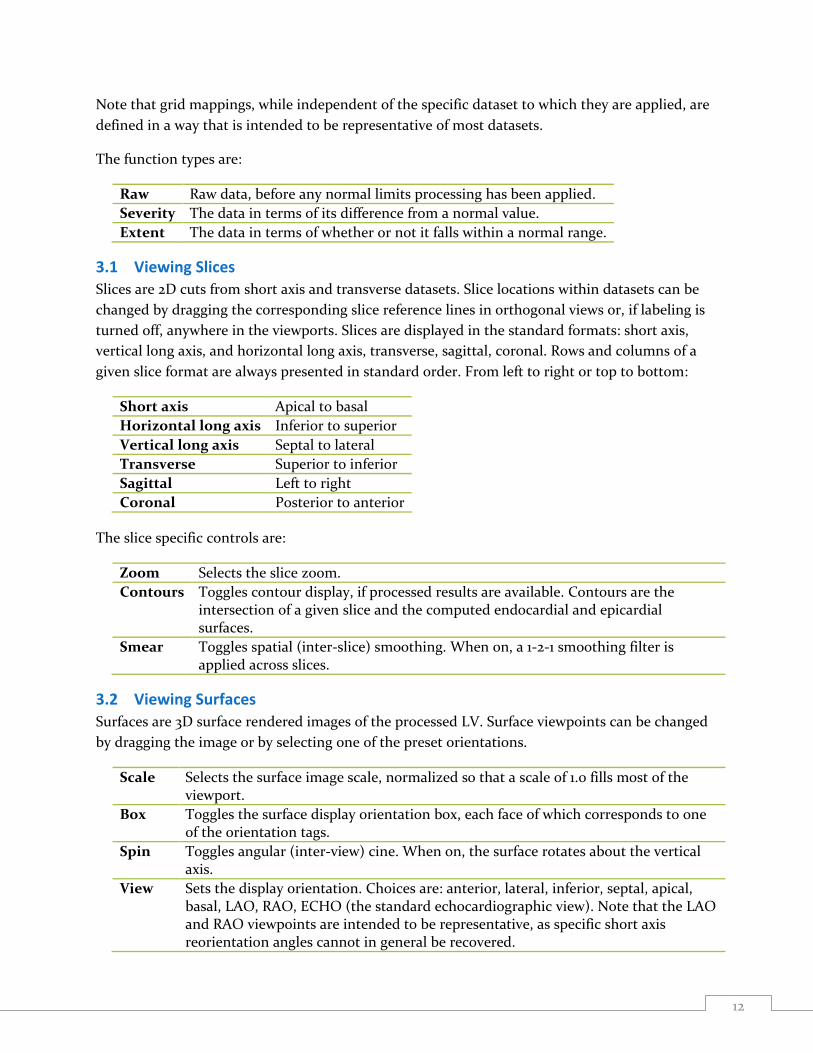
3.1 Viewing Slices
Slices are 2D cuts from short axis and transverse datasets. Slice locations within datasets can be
changed by dragging the corresponding slice reference lines in orthogonal views or, if labeling is
turned off, anywhere in the viewports. Slices are displayed in the standard formats: short axis,
vertical long axis, and horizontal long axis, transverse, sagittal, coronal. Rows and columns of a
given slice format are always presented in standard order. From left to right or top to bottom:
Short axis Apical to basal
Horizontal long axis Inferior to superior
Vertical long axis Septal to lateral
Transverse Superior to inferior
Sagittal Left to right
Coronal Posterior to anterior
The slice specific controls are:
Zoom Selects the slice zoom.
Contours Toggles contour display, if processed results are available. Contours are the intersection of a given slice and the computed endocardial and epicardial surfaces.
Smear Toggles spatial (inter-slice) smoothing. When on, a 1-2-1 smoothing filter is applied across slices.
3.2 Viewing Surfaces
Surfaces are 3D surface rendered images of the processed LV. Surface viewpoints can be changed
by dragging the image or by selecting one of the preset orientations.
Scale Selects the surface image scale, normalized so that a scale of 1.0 fills most of the viewport.
Box Toggles the surface display orientation box, each face of which corresponds to one of the orientation tags.
Spin Toggles angular (inter-view) cine. When on, the surface rotates about the vertical axis.
View Sets the display orientation. Choices are: anterior, lateral, inferior, septal, apical, basal, LAO, RAO, ECHO (the standard echocardiographic view). Note that the LAO and RAO viewpoints are intended to be representative, as specific short axis reorientation angles cannot in general be recovered.
13
Surface Selects which wall surface to display (inner, outer, both, middle, counts). The counts selection displays the mid-myocardial surface with maximal counts mapped onto it for both gated and ungated datasets.
Pins Toggles pin display, where parametric data is represented by lines extending from the surface with length proportional to magnitude.
Vessels Toggles display of the coronary vessels, previously segmented and labeled.
Fuse Registers the coronary vessels to its associated LV surface.
3.3 Viewing Polar Maps
Polar maps are 2D representations of the LV myocardium. The polar map to LV mapping is:
Center Apical
Left Septal
Right Lateral
Up Anterior
Down Inferior
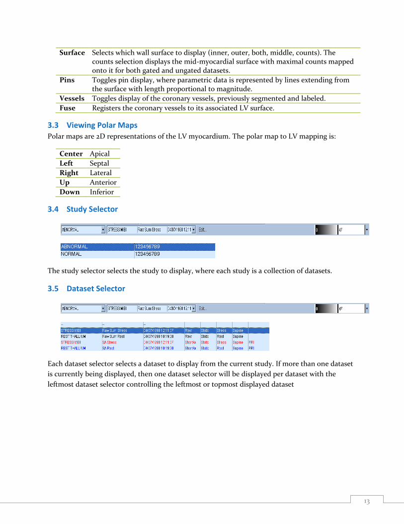
3.4 Study Selector
The study selector selects the study to display, where each study is a collection of datasets.
3.5 Dataset Selector
Each dataset selector selects a dataset to display from the current study. If more than one dataset
is currently being displayed, then one dataset selector will be displayed per dataset with the
leftmost dataset selector controlling the leftmost or topmost displayed dataset

14
3.6 Dataset Editor
Many QPS algorithms and displays require the correct categorization of datasets in order to work
correctly. In cases where automatic categorization did not work, either because dataset fields
were empty or because they did not match the criteria specified in the application defaults, the
dataset editor can be used to correctly re-categorize. It is accessed by the Edit button to the right
of the dataset selector and allows for changes to the following fields:
Sex Patient sex (can only be set for the patient, not for individual datasets).
Isotope The imaging radiopharmaceutical’s isotope.
Orientation Patient acquisition orientation.
Active Enables the dataset to be processed and displayed.
Stress Stress dataset.
Rest Rest dataset.
4Hour 4 hour (delayed) dataset.
Late 24 hour or later dataset.
Primary The default datasets to be used in reversibility computations.
AttC Attenuation corrected.
Via Viability (not always available).
Limits The perfusion normal limits to be applied.
Select OK to accept changes, Cancel to discard. If the limits field is incorrect, before changing it
first try to correct any other incorrectly assigned fields, as this should lead to the limits field being
correctly reassigned.
15
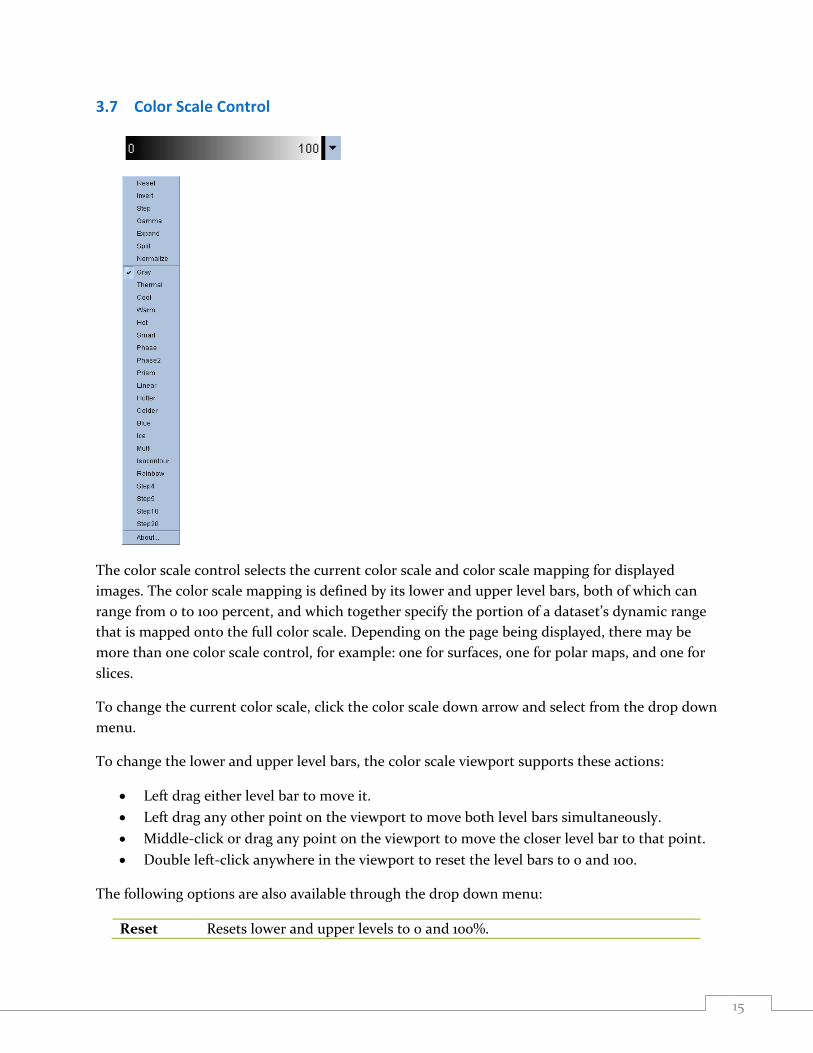
3.7 Color Scale Control
The color scale control selects the current color scale and color scale mapping for displayed
images. The color scale mapping is defined by its lower and upper level bars, both of which can
range from 0 to 100 percent, and which together specify the portion of a dataset’s dynamic range
that is mapped onto the full color scale. Depending on the page being displayed, there may be
more than one color scale control, for example: one for surfaces, one for polar maps, and one for
slices.
To change the current color scale, click the color scale down arrow and select from the drop down
menu.
To change the lower and upper level bars, the color scale viewport supports these actions:
Left drag either level bar to move it.
Left drag any other point on the viewport to move both level bars simultaneously.
Middle-click or drag any point on the viewport to move the closer level bar to that point.
Double left-click anywhere in the viewport to reset the level bars to 0 and 100.
The following options are also available through the drop down menu:
Reset Resets lower and upper levels to 0 and 100%.
16
Invert Toggles the sense of the lower and upper levels, flipping the color scale.
Step Toggles color scale discretization, making the color scale stepped.
Gamma Toggles display of the gamma control, which can be used to brighten or darken the color scale.
Expand Toggles dynamic range expansion of lower and upper levels, so that the entire image may be represented using only a portion of the color scale.
Split Toggles individual dataset color scale controls. Available only on pages with multiple datasets displayed.
Normalize Toggles automatic dataset normalization based on segmentation results.
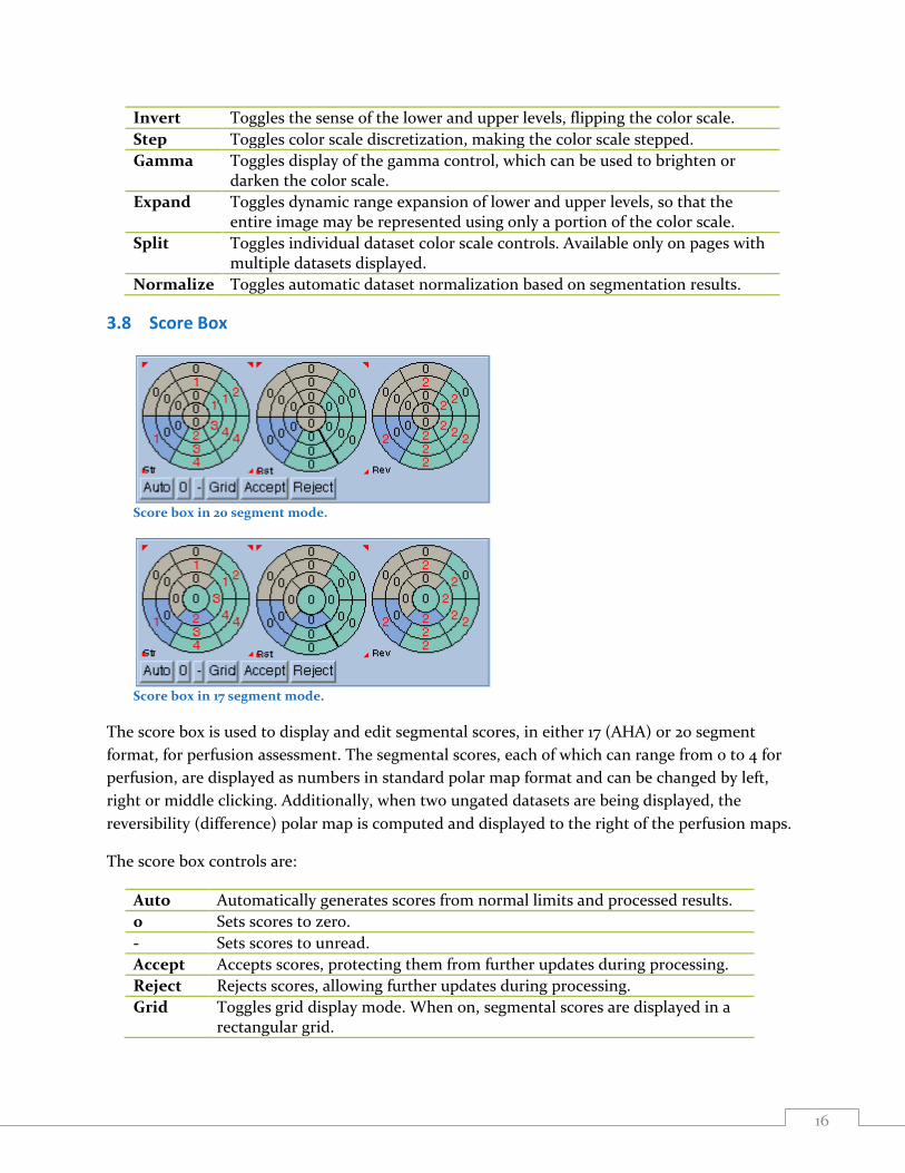
3.8 Score Box
Score box in 20 segment mode.
Score box in 17 segment mode.
The score box is used to display and edit segmental scores, in either 17 (AHA) or 20 segment
format, for perfusion assessment. The segmental scores, each of which can range from 0 to 4 for
perfusion, are displayed as numbers in standard polar map format and can be changed by left,
right or middle clicking. Additionally, when two ungated datasets are being displayed, the
reversibility (difference) polar map is computed and displayed to the right of the perfusion maps.
The score box controls are:
Auto Automatically generates scores from normal limits and processed results.
0 Sets scores to zero.
- Sets scores to unread.
Accept Accepts scores, protecting them from further updates during processing.
Reject Rejects scores, allowing further updates during processing.
Grid Toggles grid display mode. When on, segmental scores are displayed in a rectangular grid.
17
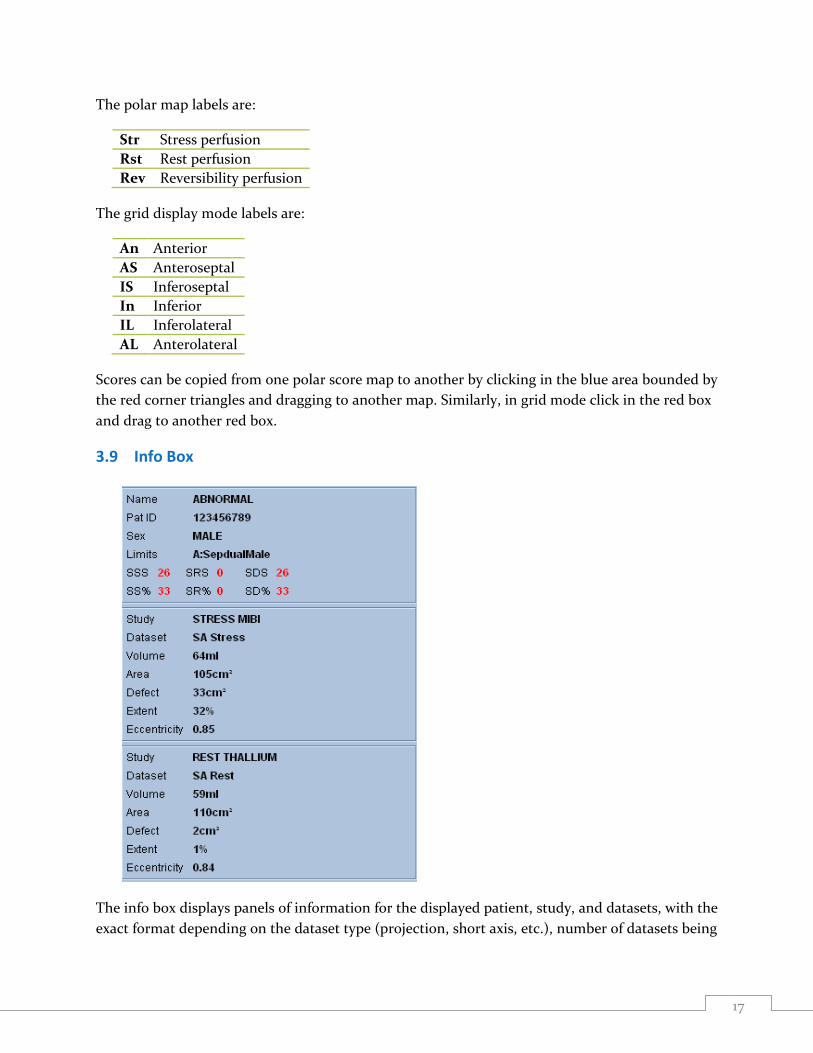
The polar map labels are:
Str Stress perfusion
Rst Rest perfusion
Rev Reversibility perfusion
The grid display mode labels are:
An Anterior
AS Anteroseptal
IS Inferoseptal
In Inferior
IL Inferolateral
AL Anterolateral
Scores can be copied from one polar score map to another by clicking in the blue area bounded by
the red corner triangles and dragging to another map. Similarly, in grid mode click in the red box
and drag to another red box.
3.9 Info Box
The info box displays panels of information for the displayed patient, study, and datasets, with the
exact format depending on the dataset type (projection, short axis, etc.), number of datasets being
18
displayed, and current page (raw, slice, etc). When multiple datasets are displayed the topmost
dataset panel corresponds to the leftmost dataset selector.
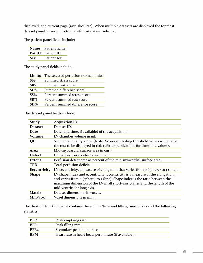
The patient panel fields include:
Name Patient name
Pat ID Patient ID
Sex Patient sex
The study panel fields include:
Limits The selected perfusion normal limits
SSS Summed stress score
SRS Summed rest score
SDS Summed difference score
SS% Percent summed stress score
SR% Percent summed rest score
SD% Percent summed difference score
The dataset panel fields include:
Study Acquisition ID.
Dataset Dataset ID.
Date Date (and time, if available) of the acquisition.
Volume LV chamber volume in ml.
QC Segmental quality score. (Note: Scores exceeding threshold values will enable the text to be displayed in red; refer to publications for threshold values).
Area Mid-myocardial surface area in cm².
Defect Global perfusion defect area in cm².
Extent Perfusion defect area as percent of the mid-myocardial surface area.
TPD Total perfusion deficit.
Eccentricity LV eccentricity, a measure of elongation that varies from 0 (sphere) to 1 (line).
Shape LV shape index and eccentricity. Eccentricity is a measure of the elongation, and varies from 0 (sphere) to 1 (line). Shape index is the ratio between the maximum dimension of the LV in all short-axis planes and the length of the mid-ventricular long axis.
Matrix Dataset dimensions in voxels.
Mm/Vox Voxel dimensions in mm.
The diastolic function panel contains the volume/time and filling/time curves and the following
statistics:
PER Peak emptying rate.
PFR Peak filling rate.
PFR2 Secondary peak filling rate.
BPM Heart rate in heart beats per minute (if available).

19
MFR/3 Mean filling rate over the first third of the end-systolic to end-diastolic phase.
TTPF Time to peak filling from end-systole.
4 Pages The pages are the central focus of QPS, with each one providing a different perspective on the
input data and processed results:
Raw Displays projection datasets, can be used for quality control and review..
Slice The slice page displays each dataset as a set of five large slices (three short axis, one vertical long axis, and one horizontal long axis), automatically or interactively selected, and can be used to examine features in detail.
Surface Displays each processed dataset as a single large 3D image of the LV surfaces, and can be used to interactively visualize features and their spatial relations to each other.
Splash Displays each dataset as multiple rows of small slices (one or two rows of short axis, one of vertical long axis, one of horizontal long axis), automatically or interactively selected. The corresponding LV surface contours can also be displayed. It is well suited for assessing function.
Views Displays each processed dataset as one or two rows of small 3D images of the LV surfaces, and can be used to interactively visualize features and their spatial relations to each other.
Results Displays an overview of processed results and perfusion analysis for one or two datasets, using slices, surfaces, polar maps, graphs, charts, and tables.
QPC Quantitative assessment of hibernating myocardium in SPECT/PET studies.
Change Direct quantification of perfusion changes between two datasets.
Fusion Fused review of SPECT/PET/CT/CTA slices in three orthogonal planes.
Snapshot Displays screen captures.
More Displays demographic data from each image dataset header, and can be used to confirm that all relevant fields are filled appropriately.
Database Allows the user to generate normal databases and limits for perfusion.

20
4.1 Raw Page
The raw page displays projection datasets, and can be used for quality control and review.
The page-specific controls are:
Lines Toggles motion reference lines.
Spin Toggles projection cine.
Rock Toggles bi-directional projection cine for sub 360 acquisitions (with spin also enabled).
Multiple Toggles multiple mode. When on, as many datasets as can fit on the screen are displayed.
Absolute Toggles absolute normalization. When on, all datasets are scaled to the same maximum value, taken across all projection datasets in the study.

21
4.2 Slice Page
The slice page displays each dataset as a set of five large slices (three short axis, one vertical long
axis, and one horizontal long axis), automatically or interactively selected, and can be used to
examine features in detail..
4.3 Surface Page
The surface page displays each processed dataset as a single large 3D image of the LV surfaces,
and can be used to interactively visualize features and their spatial relations to each other.
22
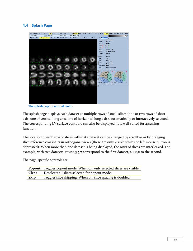
4.4 Splash Page
The splash page in normal mode.
The splash page displays each dataset as multiple rows of small slices (one or two rows of short
axis, one of vertical long axis, one of horizontal long axis), automatically or interactively selected.
The corresponding LV surface contours can also be displayed. It is well suited for assessing
function.
The location of each row of slices within its dataset can be changed by scrollbar or by dragging
slice reference crosshairs in orthogonal views (these are only visible while the left mouse button is
depressed). When more than one dataset is being displayed, the rows of slices are interleaved. For
example, with two datasets, rows 1,3,5,7 correspond to the first dataset, 2,4,6,8 to the second.
The page-specific controls are:
Popout Toggles popout mode. When on, only selected slices are visible.
Clear Deselects all slices selected for popout mode.
Skip Toggles slice skipping. When on, slice spacing is doubled.
23
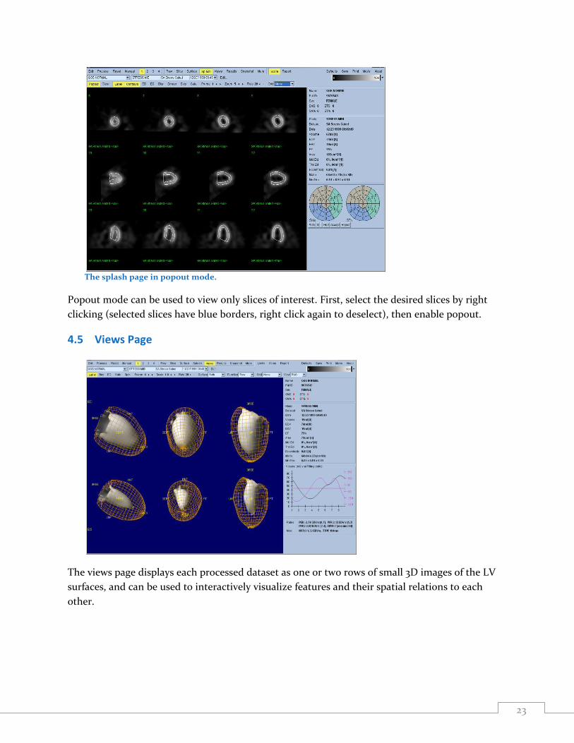
The splash page in popout mode.
Popout mode can be used to view only slices of interest. First, select the desired slices by right
clicking (selected slices have blue borders, right click again to deselect), then enable popout.
4.5 Views Page
The views page displays each processed dataset as one or two rows of small 3D images of the LV
surfaces, and can be used to interactively visualize features and their spatial relations to each
other.
24
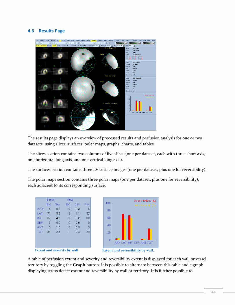
4.6 Results Page
The results page displays an overview of processed results and perfusion analysis for one or two
datasets, using slices, surfaces, polar maps, graphs, charts, and tables.
The slices section contains two columns of five slices (one per dataset, each with three short axis,
one horizontal long axis, and one vertical long axis).
The surfaces section contains three LV surface images (one per dataset, plus one for reversibility).
The polar maps section contains three polar maps (one per dataset, plus one for reversibility),
each adjacent to its corresponding surface.
Extent and severity by wall.
Extent and reversibility by wall.
A table of perfusion extent and severity and reversibility extent is displayed for each wall or vessel
territory by toggling the Graph button. It is possible to alternate between this table and a graph
displaying stress defect extent and reversibility by wall or territory. It is further possible to
25
alternate between the graph/table and the segmental function score box by toggling the Score
button.
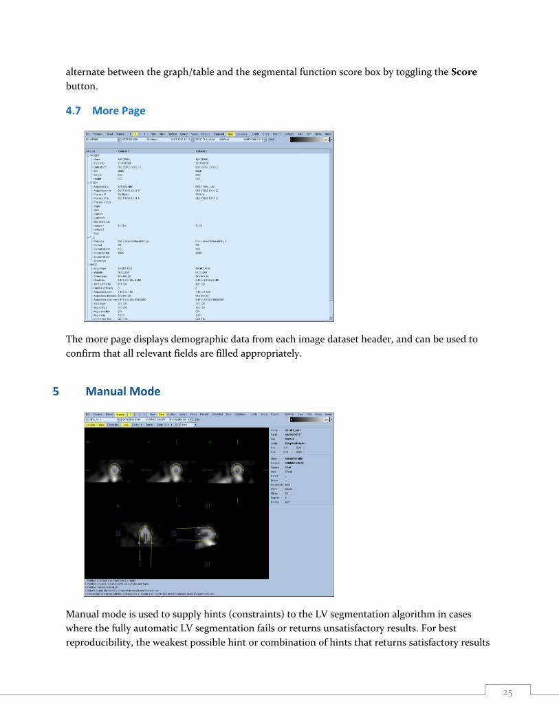
4.7 More Page
The more page displays demographic data from each image dataset header, and can be used to
confirm that all relevant fields are filled appropriately.
5 Manual Mode
Manual mode is used to supply hints (constraints) to the LV segmentation algorithm in cases
where the fully automatic LV segmentation fails or returns unsatisfactory results. For best
reproducibility, the weakest possible hint or combination of hints that returns satisfactory results
26
should be preferred. These hints are provided using essentially the same interface as the slice
page, with masking graphics (volumetric ROIs) superimposed upon the slices. The shape and
position of the masking graphics, which are initially configured to resemble an idealized LV, can
be changed by dragging its handles (the small blue boxes).
To apply manual corrections, the mask should first be shaped and positioned so that it
encompasses the LV while excluding all extra-cardiac activity (before doing so, it may be
advisable to toggle the incorrect contours off by clicking the Contours button). Then try
processing with a suitable combination of hints enabled (when the Process button is pressed all
enabled hints are applied).
The available hints, in order of increasing strength (i.e. decreasing preference) are:
Localize Restricts the initial LV search to the volume defined by the masking graphics. Use if the algorithm completely missed the LV.
Mask Restricts the entire LV segmentation algorithm to only use data within the volume defined by the masking graphics. Use to exclude extra-cardiac activity (e.g. spleen) that caused contours to be distorted.
Constrain Constrains the long axis used by the LV segmentation algorithm to lie on the end-points (apex and base) specified by the masking graphics. Use to force valveplane to be at a specific basal position.
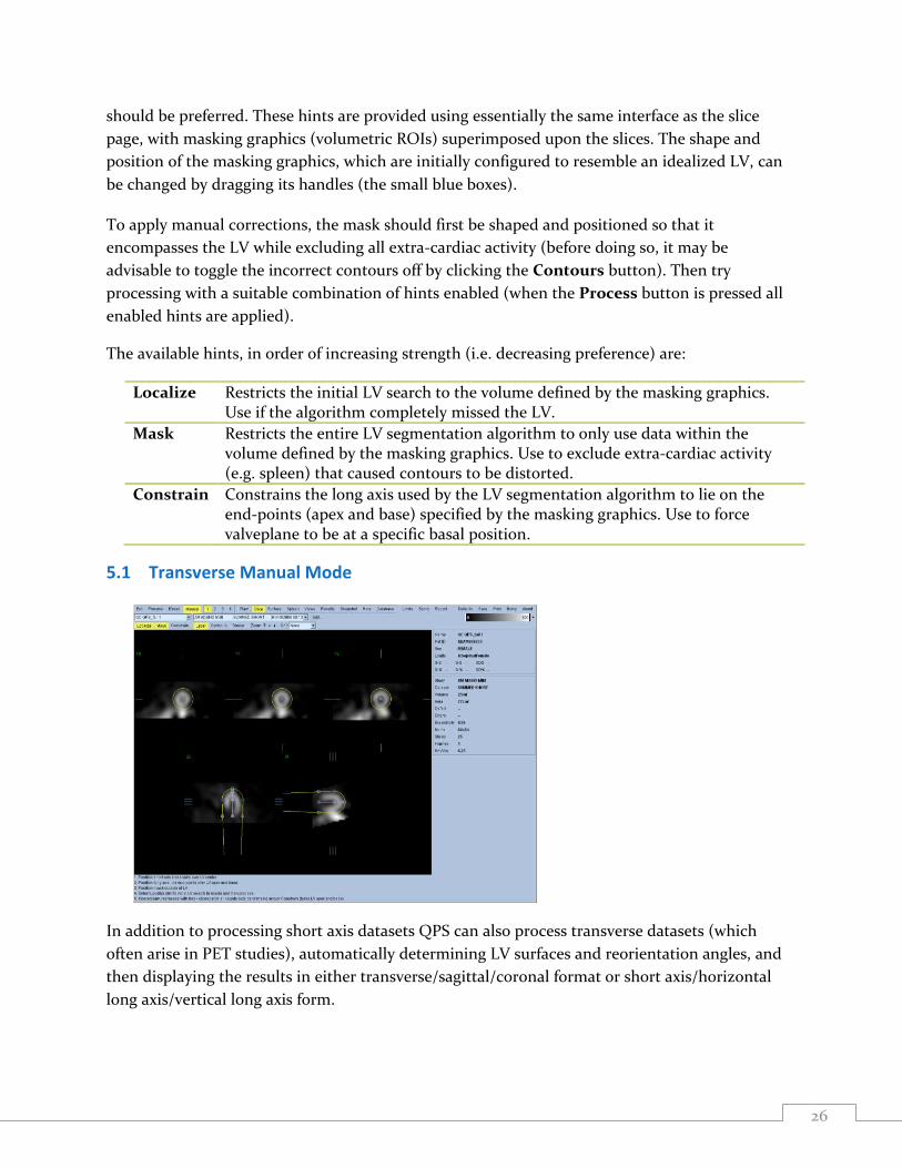
5.1 Transverse Manual Mode
In addition to processing short axis datasets QPS can also process transverse datasets (which
often arise in PET studies), automatically determining LV surfaces and reorientation angles, and
then displaying the results in either transverse/sagittal/coronal format or short axis/horizontal
long axis/vertical long axis form.
27
In cases where the automatic LV segmentation or reorientation is unsatisfactory, transverse
manual mode can be used to apply corrections to both. Transverse manual mode is the same as
short axis manual mode with the exception that reorientation may be interactively specified by
dragging the handles (small blue boxes) attached to the reorientation circles (yellow dashed
circles) so that both yellow arrows point towards the apex.
The following page specific controls are available for transverse manual mode.
Align Forces the reorientation angles to be those specified using the reorientation circles. Otherwise, they will be automatically generated.
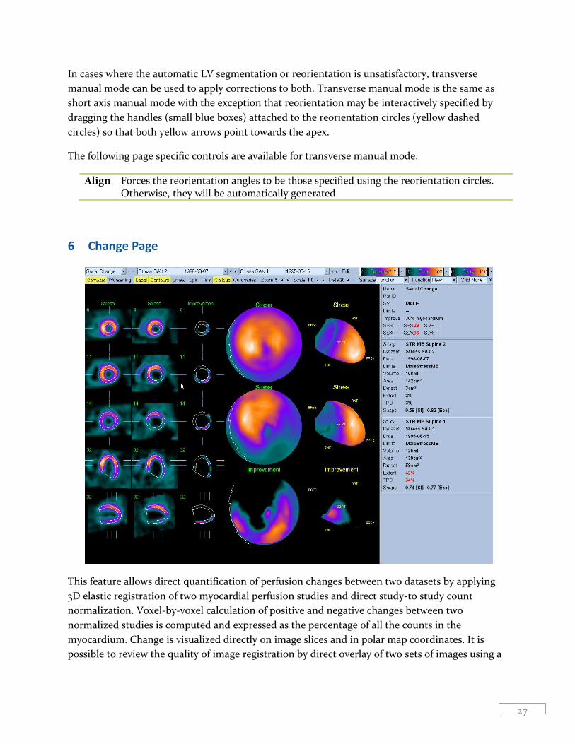
6 Change Page
This feature allows direct quantification of perfusion changes between two datasets by applying
3D elastic registration of two myocardial perfusion studies and direct study-to study count
normalization. Voxel-by-voxel calculation of positive and negative changes between two
normalized studies is computed and expressed as the percentage of all the counts in the
myocardium. Change is visualized directly on image slices and in polar map coordinates. It is
possible to review the quality of image registration by direct overlay of two sets of images using a

28
roving window on the display. No databases are required for the calculation of stress-rest changes
(ischemia) or serial (stress/stress) image changes.
The change feature can be used on stress/rest pairs to determine global ischemia measure or on
serial stress/stress pairs to evaluate changes over time (both improvement and worsening).
References: J Nucl Med. 2004 Feb;45(2):183-91
JACC Volume 45, Issue 3, Supplement 1, February 1, 2005. 1112-70, 285A.
6.1 Requirements
The change feature requires at a minimum two myocardial perfusion short axis datasets. The pairs
can be of any combination but the most useful clinically are a stress/rest pair or a stress/stress
pair. Change feature can be used for a stress/rest pair of datasets to determine global ischemia
when normal limits databases are not available, or if standard quantification results are
borderline. This feature can also be applied to pairs of data, where the stress or rest studies are
performed on different dates, to evaluate perfusion changes over time (serial changes), for
example to monitor a therapy.
6.2 Implementation
A typical sequence for using the change feature in QPS application is as follows:
1. User clicks Compare on the page control bar to apply the change algorithm. Since elastic
registration is computationally intensive it may take some time for the change results to
be reported. Hourglass is displayed to indicate the calculation progress.
2. Change results, polar map and change slice display sections are updated once the change
quantitation is performed. Change results are in % myocardium (volume).
If stress-rest studies are compared, change slice display is labeled Ischemia and change results
are displayed as Ischemia: % myocardium.
If serial stress (or serial rest) studies are compared, change results can be displayed as %
myocardium Improvement or Worsening. The default display mode is Improvement, in which the
results, change slices, and change polar maps for areas where there were positive changes are
displayed. If Worsening label is toggled, the results, change slices and change polar maps for areas
where there were negative changes are displayed. Note: the order of the serial comparison is
determined by the study date. If date is the same, the order is determined by the time of
acquisition. Therefore it is essential that the data and time of acquisition in the header are correct
for the serial change analysis.
The change feature is available in the QPS application and can be enabled to automatically apply
the change algorithm during QPS session startup by enabling (toggling on) the Change button in
the Application Options section of the Defaults Editor. Note: This will increase the startup time

29
due to change calculations being performed. If this feature is not routinely used it is best to
execute Compare “on-demand” when appropriate 2 studies are selected in the change page.
When Change is enabled in the defaults, the Compare button on the Change page is
automatically enabled indicating that the change algorithm has been applied.
6.3 Reviewing Results on the Change page
Clicking on the Change page indicator on the main toolbar will bring up the Change page. One
aspect that is quite noticeable to the user is that the Change page is very similar to the QPS
results page. Two datasets will be displayed in the Change page (the 1, 3, and 4 display datasets
options) are inactive. Change results (Ischemia, Improvement or Worsening) are displayed in the
statistic section.
Assessing Change results
The Change page provides three perfusion polar maps and three 3D parametric surfaces (stress,
rest and change-labeled as Ischemia, Improvement, or Worsening). The Function pull-down
menu contains the options “Raw”, “Severity”, and “Extent”, all of which apply to both 2D and 3D
displays. A grid of 20 or 17 segments (Segments), 3 vascular territories (Vessels) or 4 regions
(Walls) can be overlaid onto all polar maps and surfaces from the Grid pull-down menu: in the
polar maps case, the numbers associated with the overlay represent the average value of the
parameter measured by each map within the segment, territory or region in which they lie. Both
stress and rest perfusion values (or stress pairs) are normalized to 100. In addition, a slice display
of change (ischemia, improvement, or worsening) is presented where the change can be
visualized in the original slice coordinates. Note: In order to able to relate the change images and
original images it is necessary to display image contours by toggling “Contours”. The contours
displayed are that of the first study (or Stress in Stress/ Rest comparison) and are overlaid over
the coregistered second study and change images. No separate contours of rest (or second) study
are displayed during the comparison.
6.4 Controls
The following page specific controls are available:
Compare Toggling on applies the registration and change algorithm to the currently displayed pair of datasets producing the change slices and change polar map. Toggling off resets the slices and polar map.
Worsening Applicable for serial stress or serial rest comparisons only. Toggling on shows the results, change slices, and change polar maps for areas where there were negative changes or hypoperfusion.
Contours Turns contour display on and off. Contours are the intersection of a given slice and the endocardial and epicardial surfaces obtained byQPS. Note that in the change page only contours from the first study are used and are duplicated for the second study, which is registered to the first.

30
6.5 Roving Window
The roving window utility allows for quality control of the registration process. The following
describes how to use this aspect of the Change feature.
On the Change page:
1. In the slices section, with the mouse pointer on a slice image, click and hold the right
mouse button. Note: The user may zoom the images prior to performing this step using
the Zoom page control.
2. A rectangular “window” appears containing slice data as follows.
a. If the user performed step 1) on a slice in the left-most column of slices (usually a
stress dataset), the window contains slice data from the adjacent slice in the
middle column of slices (can be a rest or stress dataset).
b. If the user performed step 1) on a slice in the middle column of slices (stress or rest
dataset), the window contains slice data form the adjacent slice in the left-most
column of slices (usually a stress dataset).
c. If the user performed step 1) on a slice in the right-most column of slices (the
Change slices), the window contains slice data from the corresponding slice in the
left-most column of images (usually a stress dataset).
3. While holding the right mouse button the user can drag the window in that slice area and
verify correct registration of the slices by positioning the window over the underlying slice
data.
31
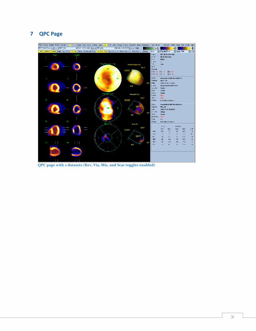
7 QPC Page
QPC page with 2 datasets (Rev, Via, Mis, and Scar toggles enabled)
32
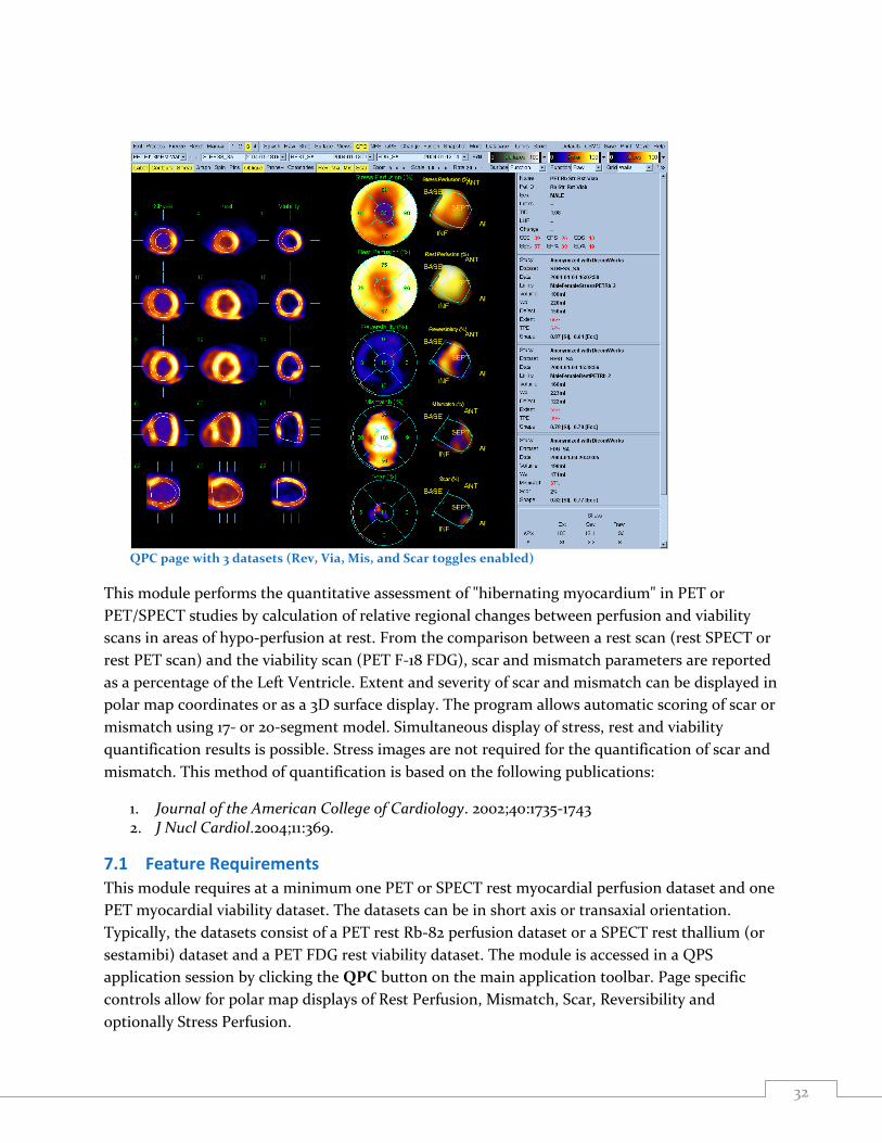
QPC page with 3 datasets (Rev, Via, Mis, and Scar toggles enabled)
This module performs the quantitative assessment of "hibernating myocardium" in PET or
PET/SPECT studies by calculation of relative regional changes between perfusion and viability
scans in areas of hypo-perfusion at rest. From the comparison between a rest scan (rest SPECT or
rest PET scan) and the viability scan (PET F-18 FDG), scar and mismatch parameters are reported
as a percentage of the Left Ventricle. Extent and severity of scar and mismatch can be displayed in
polar map coordinates or as a 3D surface display. The program allows automatic scoring of scar or
mismatch using 17- or 20-segment model. Simultaneous display of stress, rest and viability
quantification results is possible. Stress images are not required for the quantification of scar and
mismatch. This method of quantification is based on the following publications:
1. Journal of the American College of Cardiology. 2002;40:1735-1743 2. J Nucl Cardiol.2004;11:369.
7.1 Feature Requirements
This module requires at a minimum one PET or SPECT rest myocardial perfusion dataset and one
PET myocardial viability dataset. The datasets can be in short axis or transaxial orientation.
Typically, the datasets consist of a PET rest Rb-82 perfusion dataset or a SPECT rest thallium (or
sestamibi) dataset and a PET FDG rest viability dataset. The module is accessed in a QPS
application session by clicking the QPC button on the main application toolbar. Page specific
controls allow for polar map displays of Rest Perfusion, Mismatch, Scar, Reversibility and
optionally Stress Perfusion.

33
Note: The rest perfusion dataset (Rb-82, Tl-201, or Tc-99m) must have a corresponding normal
limits database.
How is the Viability Study identified?
The Viability study is identified by any one of several identifiers: (a) If the process ID field
contains FDG, F 18 or F-18 (case-insensitive), (b) if the isotope text field contains FDG, F 18 or F-18
(case insensitive), (c) if the isotope enumeration field is FDG.
7.2 Implementation
A typical processing sequence for the QPC module in is as follows:
1. User selects necessary SPECT and PET myocardial perfusion short axis datasets (and any other desired datasets for a standard QPS session, raw projections etc.) and then starts a QPS session.
2. The short axis datasets are processed by QPS to generate contours. 3. User verifies contours. 4. User clicks QPC on the QPS application main toolbar to display the QPC page. 5. User confirms correct selection of rest perfusion dataset and viability dataset in the slices
section of the QPC page. User can manually select appropriate datasets using the dataset drop-down selectors.
6. Using the page controls the user can display polar maps showing mismatch and scar by toggling “on” the Mis and/or Scar buttons.
7. If a matching stress perfusion dataset has been included in the application session the user can display it in the slices section by clicking 3 display view and selecting the stress dataset from the dataset selector drop-down ( if not already selected). Using the page controls the user can display a reversibility polar map by toggling “on” the Rev button. If appropriate stress and rest datasets are not currently selected, a difference polar map will be presented instead.
8. Depending on the datasets chosen as input to the application session the user can display
Mismatch and Scar polar maps displayed (Via, Mis and Scar enabled on Page Control Bar)
7.3 Reviewing Results on the QPC page Clicking on the QPC page indicator on the main toolbar will bring up the QPC page. One aspect
that is quite noticeable to the user is that the QPC page is very similar to the QPS results page. Up
to three datasets can be displayed in the slices section of the QPC page (the 4 display option is
inactive). The datasets most useful for this page are stress perfusion, rest perfusion and a viability
34
dataset although only rest perfusion and viability datasets are required for calculation of QPC
results.
Assessing Slices, Polar Maps and Surfaces
The QPC page provides five slice views for each dataset (up to 3 datasets can be displayed. In
addition, up to five polar maps and corresponding 3D parametric surfaces representing Stress
Perfusion, Rest Perfusion, Reversibility, Mismatch, and Scar can be displayed. The Page Control
bar provides for optimal display of slices, polar maps and 3D parametric surfaces (described in
Section 7.4). A grid of 20 or 17 segments (Segments), 3 vascular territories (Vessels) or 4 regions
(Walls) can be overlaid onto all polar maps and surfaces from the Grid pull-down menu: in the
polar maps case, the numbers associated with the overlay represent the average value of the
parameter measured by each map within the segment, territory or region in which they lie. Both
stress and rest perfusion values are normalized to 100.
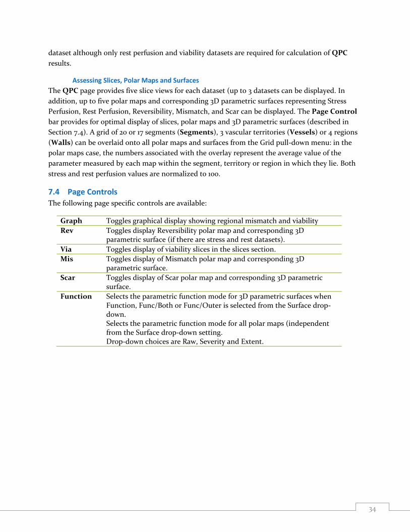
7.4 Page Controls
The following page specific controls are available:
Graph Toggles graphical display showing regional mismatch and viability
Rev Toggles display Reversibility polar map and corresponding 3D parametric surface (if there are stress and rest datasets).
Via Toggles display of viability slices in the slices section.
Mis Toggles display of Mismatch polar map and corresponding 3D parametric surface.
Scar Toggles display of Scar polar map and corresponding 3D parametric surface.
Function Selects the parametric function mode for 3D parametric surfaces when Function, Func/Both or Func/Outer is selected from the Surface drop-down. Selects the parametric function mode for all polar maps (independent from the Surface drop-down setting. Drop-down choices are Raw, Severity and Extent.
35
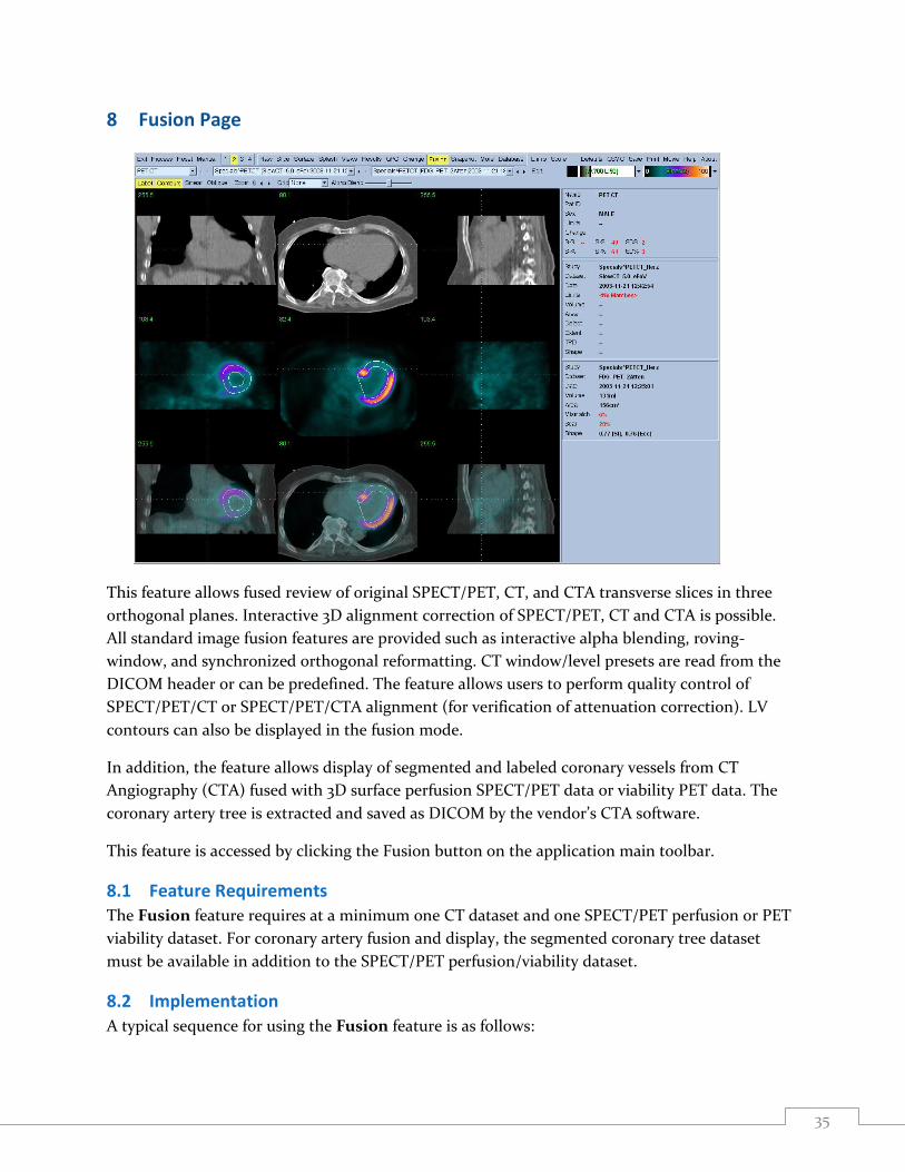
8 Fusion Page
This feature allows fused review of original SPECT/PET, CT, and CTA transverse slices in three
orthogonal planes. Interactive 3D alignment correction of SPECT/PET, CT and CTA is possible.
All standard image fusion features are provided such as interactive alpha blending, roving-
window, and synchronized orthogonal reformatting. CT window/level presets are read from the
DICOM header or can be predefined. The feature allows users to perform quality control of
SPECT/PET/CT or SPECT/PET/CTA alignment (for verification of attenuation correction). LV
contours can also be displayed in the fusion mode.
In addition, the feature allows display of segmented and labeled coronary vessels from CT
Angiography (CTA) fused with 3D surface perfusion SPECT/PET data or viability PET data. The
coronary artery tree is extracted and saved as DICOM by the vendor’s CTA software.
This feature is accessed by clicking the Fusion button on the application main toolbar.
8.1 Feature Requirements
The Fusion feature requires at a minimum one CT dataset and one SPECT/PET perfusion or PET
viability dataset. For coronary artery fusion and display, the segmented coronary tree dataset
must be available in addition to the SPECT/PET perfusion/viability dataset.
8.2 Implementation
A typical sequence for using the Fusion feature is as follows:

36
1. User selects necessary CT/CTA and SPECT/PET datasets.
2. User starts application session. Session will create contours for the SPECT/PET dataset(s).
3. Optionally, user verifies contours.
4. User clicks Fusion on the main toolbar to display the Fusion page.
5. Note: If the data comes from a Hybrid scanner and is aligned by the vendor, the Fusion
page shows “hardware fusion” on the image display in the bottom.
6. Misalignment of CT and SPECT/PET images can be visually ascertained.
8.3 Reviewing Images on the Fusion page
Clicking on the Fusion page indicator on the main toolbar will bring up the Fusion page. Two
datasets will be displayed in the Fusion page (the 1, 3, and 4 display datasets options) are inactive.
The Fusion page provides an image display area comprised of three rows and three columns. The
three rows (starting from the top) consist of NM, CT and fused images, respectively. The three
columns (starting from the left) comprise the orthogonal views, Coronal, Transverse and Sagittal,
respectively.
Visual inspection of the fused images provides an indication of the alignment between the CT
acquisition and the NM acquisition. Accurate alignment between the two acquisitions is
necessary when applying attenuation correction of PET data using CT data. The degree of
misalignment noted on visual inspection will determine if repeat imaging/processing is necessary.
Slice reference lines are provided to allow the user to change the displayed slices interactively
using a mouse. Mouse controls are described in section 8.5 below.
In addition, keyboard controls (described in section 8.6 below) allow manual alignment of mis-
registered SPECT/PET and CT data.
8.4 Controls
The following page specific controls are available:
Contours Turns contour display on and off. Contours are the intersection of a given slice and the endocardial and epicardial surfaces obtained by QPS. Note that in the change page only contours from the first study are used and are duplicated for the second study, which is registered to the first.
Alpha Blend
Sets the opacity level of SPECT/PET images on CT images in the fused image section
8.5 Mouse Controls
The following page specific mouse controls are available for interactive slice display.
Left-click, hold+drag
Left-click, hold sets the slice reference lines to the current mouse pointer position. Dragging the mouse repositions the slice reference lines on the displayed images and updates the displayed slices.
37
Middle-click, hold+drag
Allows movement of any of the nine display images within its individual display area. Releasing the middle button resets all other displayed images within their respective display areas.
Right-click, hold+drag
Enables the “Roving window” utility as described in Section 0
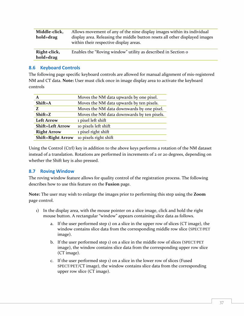
8.6 Keyboard Controls The following page specific keyboard controls are allowed for manual alignment of mis-registered
NM and CT data. Note: User must click once in image display area to activate the keyboard
controls
A Moves the NM data upwards by one pixel.
Shift+A Moves the NM data upwards by ten pixels.
Z Moves the NM data downwards by one pixel.
Shift+Z Moves the NM data downwards by ten pixels.
Left Arrow 1 pixel left shift
Shift+Left Arrow 10 pixels left shift
Right Arrow 1 pixel right shift
Shift+Right Arrow 10 pixels right shift
Using the Control (Ctrl) key in addition to the above keys performs a rotation of the NM dataset
instead of a translation. Rotations are performed in increments of 2 or 20 degrees, depending on
whether the Shift key is also pressed.
8.7 Roving Window
The roving window feature allows for quality control of the registration process. The following
describes how to use this feature on the Fusion page.
Note: The user may wish to enlarge the images prior to performing this step using the Zoom
page control.
1) In the display area, with the mouse pointer on a slice image, click and hold the right mouse button. A rectangular “window” appears containing slice data as follows.
a. If the user performed step 1) on a slice in the upper row of slices (CT image), the window contains slice data from the corresponding middle row slice (SPECT/PET image).
b. If the user performed step 1) on a slice in the middle row of slices (SPECT/PET image), the window contains slice data from the corresponding upper row slice (CT image).
c. If the user performed step 1) on a slice in the lower row of slices (Fused SPECT/PET/CT image), the window contains slice data from the corresponding upper row slice (CT image).
38
2) While holding the right mouse button the user can drag the window in that slice area and verify correct registration of the slices by positioning the window over the underlying slice data.
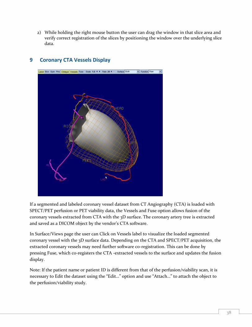
9 Coronary CTA Vessels Display
If a segmented and labeled coronary vessel dataset from CT Angiography (CTA) is loaded with
SPECT/PET perfusion or PET viability data, the Vessels and Fuse option allows fusion of the
coronary vessels extracted from CTA with the 3D surface. The coronary artery tree is extracted
and saved as a DICOM object by the vendor’s CTA software.
In Surface/Views page the user can Click on Vessels label to visualize the loaded segmented
coronary vessel with the 3D surface data. Depending on the CTA and SPECT/PET acquisition, the
extracted coronary vessels may need further software co-registration. This can be done by
pressing Fuse, which co-registers the CTA -extracted vessels to the surface and updates the fusion
display.
Note: If the patient name or patient ID is different from that of the perfusion/viability scan, it is
necessary to Edit the dataset using the “Edit…” option and use “Attach…” to attach the object to
the perfusion/viability study.
39
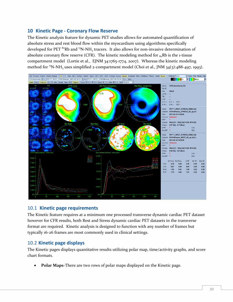
10 Kinetic Page - Coronary Flow Reserve The Kinetic analysis feature for dynamic PET studies allows for automated quantification of
absolute stress and rest blood flow within the myocardium using algorithms specifically
developed for PET 82Rb and 13N-NH3 tracers. It also allows for non-invasive determination of
absolute coronary flow reserve (CFR). The kinetic modeling method for 82Rb is the 1-tissue
compartment model (Lortie et al., EJNM 34:1765-1774, 2007). Whereas the kinetic modeling
method for 13N-NH3 uses simplified 2-compartment model (Choi et al., JNM 34(3):488-497, 1993).
10.1 Kinetic page requirements The Kinetic feature requires at a minimum one processed transverse dynamic cardiac PET dataset
however for CFR results, both Rest and Stress dynamic cardiac PET datasets in the transverse
format are required. Kinetic analysis is designed to function with any number of frames but
typically 16-26 frames are most commonly used in clinical settings.
10.2 Kinetic page displays The Kinetic pages displays quantitative results utilizing polar map, time/activity graphs, and score
chart formats.
Polar Maps-There are two rows of polar maps displayed on the Kinetic page.

40
o The polar maps displayed towards the top of the page show the absolute blood flow in
the Myocardium for the loaded datasets in ml/g/min. If both Rest and Stress dynamic
flow datasets are loaded, an additional CFR polar map showing the coronary flow
reserve is also displayed. The polar maps can be segmented into Vessels, Groups,
Walls, and Segments using the grid pull down menu. The values are averaged for the
polar map pixels for each user defined segment.
o The Polar maps displayed in the middle of the page show radiotracer activity within
the myocardium in [(Bq/ml)/Time(Sec)]. There are up to 4 polar maps displayed in
this region if both the rest and stress flow datasets are loaded. Two of the polar maps
show summed data that sums the information from all frames (Right); the remaining
two polar maps show data for the specific frame being displayed (Left).
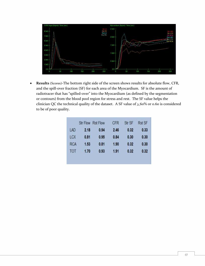
Time/Activity graphs-The time/activity curves display radiotracer activity both within
the blood pool of the right and left ventricles (left) and for the Myocardium (right).
When the Grid setting is set to Vessels, the Myocardium graph will also display the
curves for each of the 3 main coronary blood vessels (LAD, LCX, and RCA). The values in
the time/activity graphs represent absolute radiotracer activity [Bq/ml]/Time[sec].
41
Results (Scores)-The bottom right side of the screen shows results for absolute flow, CFR,
and the spill-over fraction (SF) for each area of the Myocardium. SF is the amount of
radiotracer that has “spilled-over” into the Myocardium (as defined by the segmentation
or contours) from the blood pool region for stress and rest. The SF value helps the
clinician QC the technical quality of the dataset. A SF value of > 60% or 0.60 is considered
to be of poor quality.

42
10.3 Manual Processing mode for dynamic PET data sets
Manual mode may be used to supply hints to the segmentation algorithm in cases where the fully
automatic LV segmentation fails or returns unsatisfactory results. For best reproducibility, the
weakest possible hint or combination of hints that returns satisfactory results should be preferred.
These hints are provided using essentially the same interface as the slice page, with masking
graphics (volumetric ROIs) superimposed upon the slices. The shape and position of the masking
graphics, which are initially configured to resemble an idealized LV, can be changed by dragging
its handles (the small blue boxes).
To apply manual corrections, the mask should first be shaped and positioned so that it
encompasses the LV while excluding all extra-cardiac activity (before doing so, it may be
advisable to toggle the incorrect contours off by clicking the Contours button). It may be easier
to visualize the LV on the Manual page by using longer frames (typically the last 3-6 frames of the
acquisition protocols are commonly acquired for longer durations). Time information for the
displayed frame is shown in the right side of the page next to the volume information. Then try
processing with a suitable combination of hints enabled (when the Process button is pressed all
enabled hints are applied).
The available hints, in order of increasing strength (i.e. decreasing preference) are:

43
Localize Restricts the initial LV search to the volume defined by the masking graphics. Use if the algorithm completely missed the LV.
Mask Restricts the entire LV segmentation algorithm to only use data within the volume defined by the masking graphics. Use to exclude extra-cardiac activity (e.g. spleen) that caused contours to be distorted.
Constrain Constrains the long axis used by the LV segmentation algorithm to lie on the end-points (apex and base) specified by the masking graphics. Use to force valveplane to be at a specific basal position.
As transverse data sets are often generated for PET studies, manual mode can also be used for
automatically determining reorientation angles, and then displaying the results in either
transverse/sagittal/coronal format or short axis/horizontal long axis/vertical long axis format.
In cases where the automatic LV segmentation or reorientation is unsatisfactory, transverse
manual mode can be used to apply corrections to both. Transverse manual mode is the same as
short axis manual mode with the exception that reorientation may be interactively specified by
dragging the handles (small blue boxes) attached to the reorientation circles (yellow dashed
circles) so that both yellow arrows point towards the apex.
The following page specific controls are available for transverse manual mode.
Align Forces the reorientation angles to be those specified using the reorientation circles. Otherwise, they will be automatically generated.

44
11 Database Page
The PerFusion Quant (PFQ) database page is used to create, modify, and manage normal limits
(normal databases), which are used during quantification of perfusion defects by QPS. A normal
database is defined as a collection of polar maps derived from a group of normal (typically low
likelihood) exams, where each exam is defined as a SPECT/PET myocardial perfusion dataset and
its processed results. Typically, 30-40 normal exams are used in the creation of a given database.
Multiple databases can be created and stored on one system. For example, separate databases can
be created for stress and rest datasets, or for datasets of male or female patients. Databases can
have arbitrary names as specified by the user. In order to match automatically a given database to
a particular dataset during QPS quantification of perfusion, the user can define database
attributes. This will allow assignment of a given database to a given dataset. In a typical
quantification of a standard stress/rest myocardial perfusion study, 2 separate databases will be
used: one for stress dataset and the second for the rest dataset. Using the limits menu, the user
can define a set of limits containing various normal database. The user limits can then be set as a
default in the application defaults editor.
45
The database page consists of the database control panel and database display panel. The
database control panel includes the following items: Page Specific Controls, Database Menu,
Exam Menu, Limits Menu, Current Database Attributes, and Current Database Exam List.
In the Database Display Panel the following 4 polar maps are shown: Top-left polar map-exam
highlighted in the Current Database Exam List (Patient 8 in the figure) , Top-right polar map-
current exam from the Results page, Bottom-left polar map-database Average (Normalized
Mean of all exams in the Current Database), Bottom-right polar map-database Variation
(Normalized Variation of all exams in the Current Database). Exam selection in the Current
Database Exam List can be interactively changed and polar maps for all cases included in a given
database can be quickly previewed in this manner as a quality control measure.
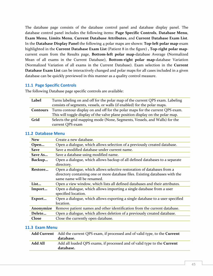
11.1 Page Specific Controls
The following Database page specific controls are available:
Label Turns labeling on and off for the polar map of the current QPS exam. Labeling consists of segments, vessels, or walls (if enabled) for the polar maps.
Contours Turns contour display on and off for the polar maps for the current QPS exam. This will toggle display of the valve plane position display on the polar map.
Grid Selects the grid mapping mode (None, Segments, Vessels, and Walls) for the current QPS exam
11.2 Database Menu
New Create a new database.
Open… Open a dialogue, which allows selection of a previously created database.
Save Save a modified database under current name.
Save As… Save a database using modified name.
Backup… Open a dialogue, which allows backup of all defined databases to a separate directory.
Restore… Open a dialogue, which allows selective restoration of databases from a directory containing one or more database files. Existing databases with the same name will be renamed.
List… Open a view window, which lists all defined databases and their attributes.
Import… Open a dialogue, which allows importing a single database from a user specified location.
Export… Open a dialogue, which allows exporting a single database to a user specified location.
Anonymize Remove patient names and other identification from the current database.
Delete… Open a dialogue, which allows deletion of a previously created database.
Close Close the currently open database.
11.3 Exam Menu
Add Current Add the current QPS exam, if processed and of valid type, to the Current database.
Add All Add all loaded QPS exams, if processed and of valid type to the Current database.
46
Delete Selected
Delete the exams selected in the Current Database Exam List from the Current Database.
Mismatch Check
When selected – a check is performed during adding of new exams to the current database to verify if the added exams match the attributes (such as Sex, Protocol) of Current Database.
Duplicate Check
When selected – a check for existing duplicates in the Current Database is performed during the process of adding new exams to the current database.
11.4 Limits Menu
Create Create a new user normal limits file.
Edit Edit an existing normal limits file
View View the contents of an existing normal limits file.
Delete
Delete an existing normal limits file.
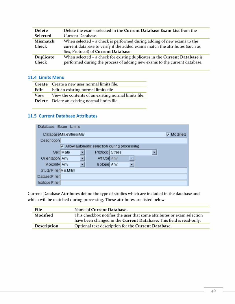
11.5 Current Database Attributes
Current Database Attributes define the type of studies which are included in the database and
which will be matched during processing. These attributes are listed below.
File Name of Current Database.
Modified This checkbox notifies the user that some attributes or exam selection have been changed in the Current Database. This field is read-only.
Description Optional text description for the Current Database.
47
Allow automatic selection during processing
When checked, it enables the automatic matching of a given database to the type of the processed exam. By selecting this option, the Current Database becomes default for the exam with matching combination of attributes (such as Sex, Protocol, Orientation etc.). Note, it is possible to have more than one matching database for a given exam. The first (alphabetically) matching will be applied in such case. By default, this option is disabled. If the user wishes that the database be matched automatically, this option should be enabled. If there is no appropriate database matched during processing, the database can be selected manually using the Dataset Editor Database field (Edit … button) on the Results page
Sex Defines the Sex attribute (Any, Female, Male) for the exams in the Current Database
Protocol Defines the acquisition protocol (Any, Stress, Rest) for the exams in the Current Database
Orientation Defines patient orientation (Supine, Prone, Any) for the exams in the Current Database
Isotope Defines the Isotope for the exams in the Current Database. Currently not used.
Att Cor Defines the Attenuation correction attribute (AC, NAC, Any) for the exams in the Current Database. Currently not used.
Study Filter Text string to be matched in the Study header field of the exams included in the Current Database.
Dataset Filter Text string to be matched in the Dataset header field of the exams included in the Current Database.
Isotope Filter Text string to be matched in the Isotope header field of the exams included in the Current Database. This is an alternative method for matching the databases by isotope during QPS processing.
11.6 QPS Database Procedures
Creating a New Database
These are steps to follow when creating normal databases:
1. Select all exams, which should be included in the new database and load all these patients
in the QPS program. These should be normal short-axis myocardial perfusion datasets of
low-likelihood patients.
2. Make sure that all datasets are processed by QPS, that all the contours* are defined
correctly, and that there are no obvious perfusion defects in the images.
3. Go to the database page and from the Database Menu, select New, which will clear all the
attribute fields in the Current Database Attributes panel.
4. From the Exam Menu select Add All. This will populate the Current Database Exam List.
5. Specify all required database attributes. Note that if “Any” is selected for a particular
attribute, the program will not consider this parameter during auto-matching when
running QPS.
48
6. If you like the created database to become default for perfusion quantification of exams
with a given combination of attributes, enable Allow automatic selection during
processing option. Note that if multiple matching databases are available the program will
produce message "Multiple matches" during the quantification. In such a case user must
select the desired database manually.
7. To anonymize the database and remove all patient information from the created database,
select Anonymize from the Database Menu. Generic patient names will appear in the
Current Database Exam list.
8. From the Database Menu select Save As... This will bring up a dialogue in which existing
database names are shown. Type in a new name in the text-box below the list of Database
names and Click OK.
* The user must verify correct contour creation. If contours appear too long, too short or
do not encompass the myocardium, they should be manually adjusted and saved.
Incorrect contours generated for the normal limits population will degrade the
quantification results when applied to clinical studies.
Adding Patients to a Database
1. Start QPS with the studies to be added.
2. Make sure that all patients are processed and contours for all studies are defined correctly.
3. From the Database Menu, select Open… and select the database to modify.
4. From the Exam Menu, select either Add Current to add the current patient, or Add All to
add all currently open patients.
5. From the Database Menu, select Save. This will overwrite the selected database with the
modified database, which includes additional patients.
Removing Patients from a Database
1. From the Database Menu, select Open…, and select the database to modify.
2. Select the patient(s) to delete from the database exam list.
3. From the Exam Menu select Delete Selected. This will update the database exam list.
4. From the Database Menu, select Save. This will overwrite the selected database with the
modified database which does not include deleted patients.
Creating a New Normal Limits File
1. From the Limits Menu, select Create...
2. From the Create Limits window, select Add to open the Limits Database selection
window.
3. From the Limits Database window, select a database to add.
4. Repeat step 3 until all database files required have been added.
5. From the Create Limits window, select Save to open the Save Limits window
6. From the Save Limits window, enter an appropriate name for this limits file and click OK.
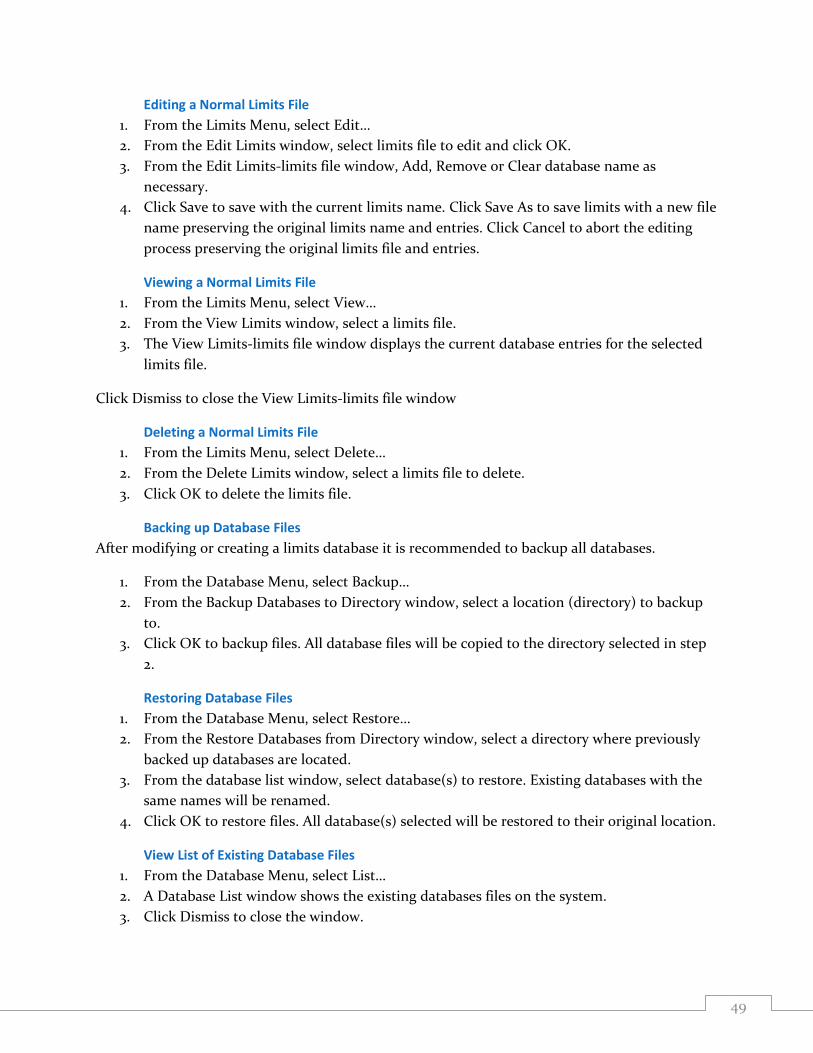
49
Editing a Normal Limits File
1. From the Limits Menu, select Edit…
2. From the Edit Limits window, select limits file to edit and click OK.
3. From the Edit Limits-limits file window, Add, Remove or Clear database name as
necessary.
4. Click Save to save with the current limits name. Click Save As to save limits with a new file
name preserving the original limits name and entries. Click Cancel to abort the editing
process preserving the original limits file and entries.
Viewing a Normal Limits File
1. From the Limits Menu, select View…
2. From the View Limits window, select a limits file.
3. The View Limits-limits file window displays the current database entries for the selected
limits file.
Click Dismiss to close the View Limits-limits file window
Deleting a Normal Limits File
1. From the Limits Menu, select Delete…
2. From the Delete Limits window, select a limits file to delete.
3. Click OK to delete the limits file.
Backing up Database Files
After modifying or creating a limits database it is recommended to backup all databases.
1. From the Database Menu, select Backup…
2. From the Backup Databases to Directory window, select a location (directory) to backup
to.
3. Click OK to backup files. All database files will be copied to the directory selected in step
2.
Restoring Database Files
1. From the Database Menu, select Restore…
2. From the Restore Databases from Directory window, select a directory where previously
backed up databases are located.
3. From the database list window, select database(s) to restore. Existing databases with the
same names will be renamed.
4. Click OK to restore files. All database(s) selected will be restored to their original location.
View List of Existing Database Files
1. From the Database Menu, select List…
2. A Database List window shows the existing databases files on the system.
3. Click Dismiss to close the window.

50
12 ARG (Automatic Report Generation)
Integration of ARG (Automatic Report Generator) provides the ability within QPS to create, edit,
sign, review, archive, and share customizable, consistency-checked, reports. A reporting pane and
a few extra dialogs have been added to QPS for this purpose. ARG is enabled by the Report button
on the right hand side of the top row of buttons. When on, the info box is replaced by the ARG
panel.
12.1 Starting QPS with ARG
ARG will automatically match the identifying information contained in the image headers with
existing (previously saved) studies. If an existing study is found, then it is possible to modify the
data or view the report associated with that study. If no study is matched, then ARG will
automatically create a new study. This new study will not get permanently saved to the database
until the Save button is clicked.
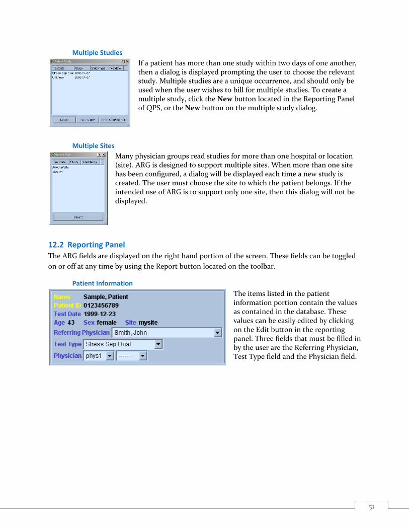
51
Multiple Studies
If a patient has more than one study within two days of one another, then a dialog is displayed prompting the user to choose the relevant study. Multiple studies are a unique occurrence, and should only be used when the user wishes to bill for multiple studies. To create a multiple study, click the New button located in the Reporting Panel of QPS, or the New button on the multiple study dialog.
Multiple Sites
Many physician groups read studies for more than one hospital or location (site). ARG is designed to support multiple sites. When more than one site has been configured, a dialog will be displayed each time a new study is created. The user must choose the site to which the patient belongs. If the intended use of ARG is to support only one site, then this dialog will not be displayed.
12.2 Reporting Panel The ARG fields are displayed on the right hand portion of the screen. These fields can be toggled
on or off at any time by using the Report button located on the toolbar.
Patient Information
The items listed in the patient information portion contain the values as contained in the database. These values can be easily edited by clicking on the Edit button in the reporting panel. Three fields that must be filled in by the user are the Referring Physician, Test Type field and the Physician field.
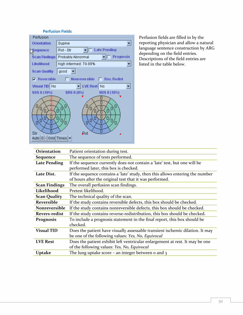
52
Perfusion Fields
Perfusion fields are filled in by the reporting physician and allow a natural language sentence construction by ARG depending on the field entries. Descriptions of the field entries are listed in the table below.
Orientation Patient orientation during test.
Sequence The sequence of tests performed.
Late Pending If the sequence currently does not contain a ‘late’ test, but one will be performed later, this box is checked.
Late Dist. If the sequence contains a ‘late’ study, then this allows entering the number of hours after the original test that it was performed.
Scan Findings The overall perfusion scan findings.
Likelihood Pretest likelihood.
Scan Quality The technical quality of the scan.
Reversible If the study contains reversible defects, this box should be checked.
Nonreversible If the study contains nonreversible defects, this box should be checked.
Revers-redist If the study contains reverse-redistribution, this box should be checked.
Prognosis To include a prognosis statement in the final report, this box should be checked.
Visual TID Does the patient have visually assessable transient ischemic dilation. It may be one of the following values: Yes, No, Equivocal
LVE Rest Does the patient exhibit left ventricular enlargement at rest. It may be one of the following values: Yes, No, Equivocal
Uptake The lung uptake score – an integer between 0 and 3
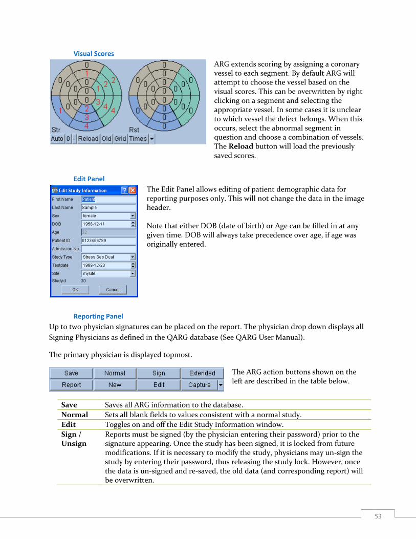
53
Visual Scores
ARG extends scoring by assigning a coronary vessel to each segment. By default ARG will attempt to choose the vessel based on the visual scores. This can be overwritten by right clicking on a segment and selecting the appropriate vessel. In some cases it is unclear to which vessel the defect belongs. When this occurs, select the abnormal segment in question and choose a combination of vessels. The Reload button will load the previously saved scores.
Edit Panel
The Edit Panel allows editing of patient demographic data for reporting purposes only. This will not change the data in the image header. Note that either DOB (date of birth) or Age can be filled in at any given time. DOB will always take precedence over age, if age was originally entered.
Reporting Panel
Up to two physician signatures can be placed on the report. The physician drop down displays all
Signing Physicians as defined in the QARG database (See QARG User Manual).
The primary physician is displayed topmost.
The ARG action buttons shown on the left are described in the table below.
Save Saves all ARG information to the database.
Normal Sets all blank fields to values consistent with a normal study.
Edit Toggles on and off the Edit Study Information window.
Sign / Unsign
Reports must be signed (by the physician entering their password) prior to the signature appearing. Once the study has been signed, it is locked from future modifications. If it is necessary to modify the study, physicians may un-sign the study by entering their password, thus releasing the study lock. However, once the data is un-signed and re-saved, the old data (and corresponding report) will be overwritten.

54
Report Displays the PDF report.
New Creates a New (multiple) study for this patient.
Extended Opens the extended editor, which permits editing of the dictation, history and ECG sections.
Capture Captures the current screen to save in report. (Ctrl+Shift+P will also capture the current screen. The key combination is useful if the ARG Panel is not desired in the screen capture).
Extended Editor
The Extended editor contains areas for dictation, history, ECG, recipients and Previous studies. Each study may have a main dictation associated with it, in addition to a history dictation. The dictation is free text that is included on the report cover letter. The dictation editor is designed to make this process as efficient as possible. ARG includes powerful built-in macros and a very flexible custom code editor. For details on the History, ECG and Recipients pane reference the QARG manual. Note that if QARG has not been purchased only the dictation screen will be visible.
Dictation
Two powerful macros are included on the dictation editor. The buttons for these macros are
located directly underneath the Custom Codes title in the Dictation Editor window beside the
Refresh button.
Auto An automatic dictation is used by default. This dictation updates real-time as fields are modified. The automatic dictation is shown in blue. Note that text can be added before or after the automatic dictation without affecting the behavior of the auto dictation. You may alter or remove the automatic dictation at any time simply by editing it. Note that once the automatic sentence(s) have been modified then the dictation will no longer be updated automatically. To re-enable the automatic dictation, click the Auto button.

55
Comparison If the patient is returning for a follow-up visit, the Comparison button is enabled. If this is the case then the signing physician should mention any changes (or no change) since the patient’s last visit. ARG will provide a warning if no mention is made. Clicking the comparison button will initialize the comparison sentence. ARG matches the previous study based on patient ID. If the patient ID was mistyped in the original study, it must be changed before ARG can auto match. Of course you may also manually enter the old study date and ARG will be able to auto-match any future studies. For more information on editing the comparison sentence or viewing raw changes, refer to the dictation section in the QARG manual.
Refresh Refreshes the list of codes in the database.
Custom Codes Custom codes are simple macros that provide a mechanism to store frequently typed sentences. Codes are made up of a code-key (small word describing the code) and code-value (text which is appended to the dictation). Codes are accessed by highlighting the code-key and clicking the Append/Add button, double clicking a code-key or typing @code-key in the dictation editor. Please see the Custom Code Manager section in the QARG User Manager for details regarding customization of these codes.
Previous Study
The previous study pane gives a very informative comparison of the patient’s previous studies.
From this pane you can view how the patient was reported in previous visits.

56
Consistency Checks
ARG contains a collection of checks resulting in various notifications of errors and warnings.
These checks ensure that the report data is consistent.
For Example: If ‘Normal’ was entered for overall perfusion scan findings and a large defect exists
in the visual scores, then an error will occur. Most checks can be viewed directly from the ARG
interface by looking at the color of the field name (field inconsistencies resulting in errors are
labeled in red, warnings in yellow). Descriptions of errors and warning are displayed in the Errors
and Warnings window (shown below) after clicking the Save button.
Critical Errors and Warnings
Critical errors prevent the report from being saved. These fields show up red in the ARG panel and are listed next to a check box in the errors and warning dialog. Most critical errors deal with the absence of required data; however some are due to major inconsistencies with the data. If errors exist in the report it is possible to continue, however the errors must be acknowledged by clicking the checkbox next to the error. Clicking the checkbox will accept the error for the current study only. To permanently disable (hide) and error right click the error and select ‘Add consistency check to blacklist.
Warnings do not prevent the report from being saved. However the physician must review them and explicitly choose to ignore them prior to saving. Theoretically, warnings should not be allowed. However, in some circumstances the inconsistency should be allowed (i.e.: the patient had a bypass surgery). Ignoring warnings should be done scarcely and only after careful consideration.
Hiding unwanted consistency checks
Users may disable errors and warnings that are irrelevant to their site by right clicking the
consistency check once the dialog is opened. This moves the consistency check to a “hidden”
group. The consistency check can be re-enabled by right clicking on the error inside the black
listed group.

57
13 Prone-Supine (Prone+) Quantification
Prone-supine (Prone+) quantification allows quantification of perfusion on prone images as well
as combined quantification of prone/supine datasets by applying heuristic rules which allow
automatic elimination of image artifacts based on the relative defect locations on prone and
supine images.
Reference: Nishina H, Slomka, PJ, Abidov AA, Yoda S, Akincioglu, C, Kang, X, Cohen, I, Hayes,
SW, Friedman, JD, Germano, G, Berman, DS.Combined Supine and Prone Quantitative
Myocardial Perfusion SPECT: Method Development and Clinical Validation in Patients with no
Known Coronary Artery Disease. (In Press J Nucl Med).
13.1 Feature Requirements
The Prone-Supine (Prone+) quantification feature requires at a minimum one supine perfusion
dataset and one prone perfusion dataset from the same patient/study. This feature is available in
the Results page and is enabled by toggling on the Prone+ button of the page control bar.
13.2 Implementation
A typical sequence for using the Prone+ feature in the QPS application is as follows:
58
1. User selects necessary myocardial perfusion short axis datasets (and any other desired
datasets for a standard QPS session, raw projections etc.) and then starts a QPS session.
2. The short axis datasets are processed by QPS to generate contours.
3. User verifies contours.
4. User displays the Results page.
5. User clicks Prone+ button to apply Prone-supine quantification algorithm and display
results. Results are displayed in the statistics section.
6. The application of the Prone+ feature is indicated in the statistics section of the Results
page and in the change of defect size/location (if any) on the Stress and Reversibility polar
maps.
Notes:
1. When the Prone+ feature is been enabled in the Results page it remains in effect for all other pages displaying perfusion results in the statistics section (Surface, Splash, etc.).
2. The Prone+ feature can be automatically enabled by toggling it on in the Application Defaults window, Application Options section and then saving the defaults settings. In this manner, the Prone+ algorithm will be applied during processing of perfusion datasets for all subsequent QPS sessions.
14 Saving Results Processing results can be saved from within the QPS application for later recall. This feature
allows manually-adjusted contours and visual scores to be saved in order to avoid repeating this
operator-dependent step. When results are saved, all datasets pertaining to the study being saved
are associated with the results file, which becomes a self-contained entity. Transferring the results
file without any other datasets to another system (e.g., using a DICOM transfer mechanism on
platforms supported by QPS) is sufficient to retain all necessary information. At this time only
transfers to a system that uses the same vendor platform is fully supported, though
interoperability between vendors may be possible if CSMC application versions match.
To save results for one or more studies, follow these steps:
1. Select your study(ies) and start your application. 2. Review the results of the study(ies) and adjust contours and/or scores if necessary. 3. Click the Save button to open the Save Results dialog. 4. Click the Results tab to display save options. See figure below. 5. If so desired, enter a description in the Dataset field (this field may have a different name
on some platforms). 6. Click Save Current to save the currently displayed study or click Save All to save all the
selected studies currently loaded. As multi-study or multi-patient processing may not be available on all platforms, on some systems Save Current and Save All will perform the same task.

59
Save Results with Results tab selected
Note: the PowerPoint tab may not be present in all software configurations.
15 PowerPoint Integration The PowerPoint save feature is a useful tool that allows saving a set of images and results along
with a batch file. The batch file launches the QPS application and loads the images and results.
This is useful for showing case studies within a Microsoft PowerPoint presentation. PowerPoint
integration is supported in Office 2000 SR1a and above.
To save a study for showing in a PowerPoint presentation, follow these steps:
1. Select your study(ies) and start your application. 2. Review the results of the study(ies) on the display page you wish to save (eg. Slice page)
and make changes as necessary (intensity/color scale, zoom, frame rate settings etc.). The changes applied will be automatically saved as the default setting for the study(ies).
3. Click the Save button to open the Save Results dialog. 4. Click the PowerPoint tab to display save options. See figure below. 5. Click Browse to select a directory to store the images and batch file. 6. Type a name in the Filename text area 7. Click Save Current to save the currently displayed study or click Save All to save all the
selected studies for the current application session.

60
Save Results with PowerPoint tab selected
15.1 Description of Saved Files Three files per study will be saved and have extensions of “vbs”, “gsi” and "xml". The “vbs” file is a
Visual Basic script file that will launch the QPS application and load the corresponding “gsi” data
file along with the "xml" file containing the saved default settings for the study(ies).
15.2 Launching application studies from PowerPoint
Studies must be saved using the procedure in the preceding section in order to use this
PowerPoint feature.
To create a slide that will launch an application (QPS) study session follow these steps.
1. Open PowerPoint and insert a new slide. 2. Under the Slide Show menu drop-down, select Action Buttons and choose an action
button graphic from the list. 3. Draw the action button on the slide. An Action Settings dialog window should be
displayed when finished drawing. Optionally, right-click on the action button and select Properties to bring up the Action Settings dialog.
4. In the Action Settings dialog click the Run program toggle. 5. Using the Browse command, locate the “vbs” file and select it. The Files of type selection
in the browse window may have to be changed from Programs (*.exe) to All Files (*.*). 6. Click OK. 7. Launch the slide show for the current slide and click the action button to verify correct
launching of the study. 8. Adding a text description beside the Action button will aid in reminding what the study
was about during a presentation.

61
Patient XYZ showing low EF post
exercise
Patient ABC showing normal EF post
exercise with ischemic changes on
perfusion study
PowerPoint slide with Action button
16 Saving Screen Captures and Printing Snapshots of the application’s screens can be saved by clicking the Print button. These screen
captures include the information box to the right of the main viewport, but not the application
controls at the top of the application’s main window. Screen captures can be saved either to the
host system’s image database (if supported by the host system), to a file (always available), or
printed to a Windows printer (if available). On DICOM-based systems, snapshots are saved as
true-color DICOM secondary captures (SC). Proprietary formats may be used for other platforms,
but exporting screen captures as DICOM SCs is always an option when saving a file to the file
system as opposed to saving to the image database.
To save a screen capture, follow these steps:
1. Select your study(ies) and start your application. 2. Configure the screen as desired (e.g., process the data, change the selected dataset, adjust
the zoom factor, select a different color scale, etc…). 3. Click the Print button to open the Print dialog. 4. Click the Database, File, or Printer tab as appropriate. See settings sections below. Fill
out or select the appropriate information. 5. Select labeling options. See “Labeling” section below. 6. If so desired, enter a description in the Series Description or Dataset field (this field
may have a different name depending on the platform). 7. Click OK to save or print the screen capture or click Cancel to cancel the task.
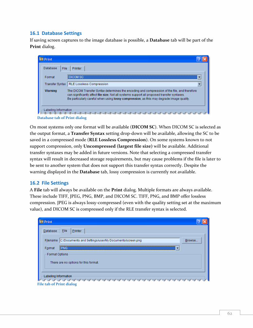
62
16.1 Database Settings
If saving screen captures to the image database is possible, a Database tab will be part of the
Print dialog.
Database tab of Print dialog
On most systems only one format will be available (DICOM SC). When DICOM SC is selected as
the output format, a Transfer Syntax setting drop-down will be available, allowing the SC to be
saved in a compressed mode (RLE Lossless Compression). On some systems known to not
support compression, only Uncompressed (largest file size) will be available. Additional
transfer syntaxes may be added in future versions. Note that selecting a compressed transfer
syntax will result in decreased storage requirements, but may cause problems if the file is later to
be sent to another system that does not support this transfer syntax correctly. Despite the
warning displayed in the Database tab, lossy compression is currently not available.
16.2 File Settings
A File tab will always be available on the Print dialog. Multiple formats are always available.
These include TIFF, JPEG, PNG, BMP, and DICOM SC. TIFF, PNG, and BMP offer lossless
compression. JPEG is always lossy-compressed (even with the quality setting set at the maximum
value), and DICOM SC is compressed only if the RLE transfer syntax is selected.
File tab of Print dialog

63
Note that the Format Options panel will only display controls if the format has optional settings.
These settings are a Quality slider for JPEG (quality can be set from 40 to 100, with 40 providing
the lowest image quality and 100 the highest image quality) and a Transfer Syntax setting for
DICOM SC (see previous section for restrictions on transfer syntaxes). All output file formats
except for DICOM SC shall be water marked to indicate that they are not for diagnostic purposes.
16.3 Printer Settings
A Printer tab will always be available on the Print dialog. The currently selected printer is listed
under Selected printer. To change to a different printer, or to edit the properties of the printer
click the Setup… button. This will open the operating system’s Print dialog that will allow the
selection of a different printer and a number of other options (on Microsoft Windows, these
options include the number of copies). On Windows, clicking Print in this dialog will cause
printing to happen immediately. Alternatively, one may click OK in the QPS Print dialog to print,
or Cancel to abort the operation.
File tab of Print dialog
16.4 Labeling The bottom portion of the Print dialog remains the same no matter what tab is selected. This
portion of the dialog is dedicated to image labeling. On DICOM-based systems a Series
Description and Comment can be entered. On other systems these fields may have a different
name or be absent altogether, depending on what fields the proprietary host platform supports.
These fields are meant to allow for the identification of the screen capture when listed in a typical
medical image database browser.
The Datasets section lists all datasets present on the current page. For each dataset acquisition
and processing information are listed, along with image generation time. This allows for the
identification of the datasets. The Operator and Institution fields are filled in automatically
from the dataset headers if available, otherwise they can be edited before printing. If the Include a
dataset legend checkbox is checked, each dataset on the printed screen will be identified by its
designation letter (A, B, or C in the example below), and a legend that includes the information in
the table will be added at the bottom of the printed or saved output. The legend table will also
include patient information (name, patient ID, date of birth) unless anonymization is enabled,
and dataset orientation and laterality (as provided by the dataset headers).

64
Labeling section of Print dialog
Note that the Format Options panel will only display controls if the format has optional settings.
These settings are a Quality slider for JPEG (quality can be set from 40 to 100, with 40 providing
the lowest image quality and 100 the highest image quality) and a Transfer Syntax setting for
DICOM SC (see previous section for restrictions on transfer syntaxes).
17 Saving Movies Movies of the application’s screens can be saved by clicking the Movie button. These movies only
include the relevant portion of the viewport as decided by each application for each page, and
does not include the information box to the right of the main viewport or the application controls
at the top of the application’s main window. Movies can be saved either to the host system’s
image database (if supported by the host system), or to a file (always available). On DICOM-based
systems, movies are saved as true-color DICOM multi-frame secondary captures (MFSC).
Proprietary formats may be used for other platforms, but exporting screen captures as DICOM
MFSCs can be an option when saving a file to the file system as opposed to saving to the image
database, unless the platform is know to not support MFSCs, in which case the option is disabled
to avoid creating files that the host system cannot handle.
When generating a movie, note that the final frame rate of the movie will vary with the
application’s Rate setting in the top application controls and attempt to match this rate. For
example, to create a faster movie of a beating heart, increase the Rate setting.
The application will pick automatically how the movie will be generated, i.e., by gating the image
or displaying a rotating image, based on the current page selection.
To save a screen capture, follow these steps:

65
1. Select your study(ies) and start your application. 2. Configure the screen as desired (e.g., process the data, change the selected dataset, adjust
the zoom factor, select a different color scale, etc…). 3. Click the Movie button to open the Movie dialog. 4. Click the Database or File tab as appropriate. See settings sections below. Fill out or
select the appropriate information. 5. Select labeling options. See “Labeling” section below. 6. If so desired, enter a description in the Series Description or Dataset field (this field
may have a different name depending on the platform). 7. Click OK to save the movie or click Cancel to cancel the task.
17.1 Database Settings If saving screen captures to the image database is possible, a Database tab will be part of the
Print dialog.
Database tab of Print dialog
On most systems only one format will be available (DICOM SC). When DICOM SC is selected as
the output format, a Transfer Syntax setting drop-down will be available, allowing the SC to be
saved in a compressed mode (RLE Lossless Compression). On some systems known to not
support compression, only Uncompressed (largest file size) will be available. Additional
transfer syntaxes may be added in future versions. Note that selecting a compressed transfer
syntax will result in decreased storage requirements, but may cause problems if the file is later to
be sent to another system that does not support this transfer syntax correctly. Despite the
warning displayed in the Database tab, lossy compression is currently not available.
17.2 File Settings A File tab will always be available on the Movie dialog. Multiple formats are usually available.
These include AVI and DICOM SC. AVI offers lossless or lossy compression, depending on the
codec (coder/decoder) used. DICOM SC is compressed only if the RLE transfer syntax is selected.
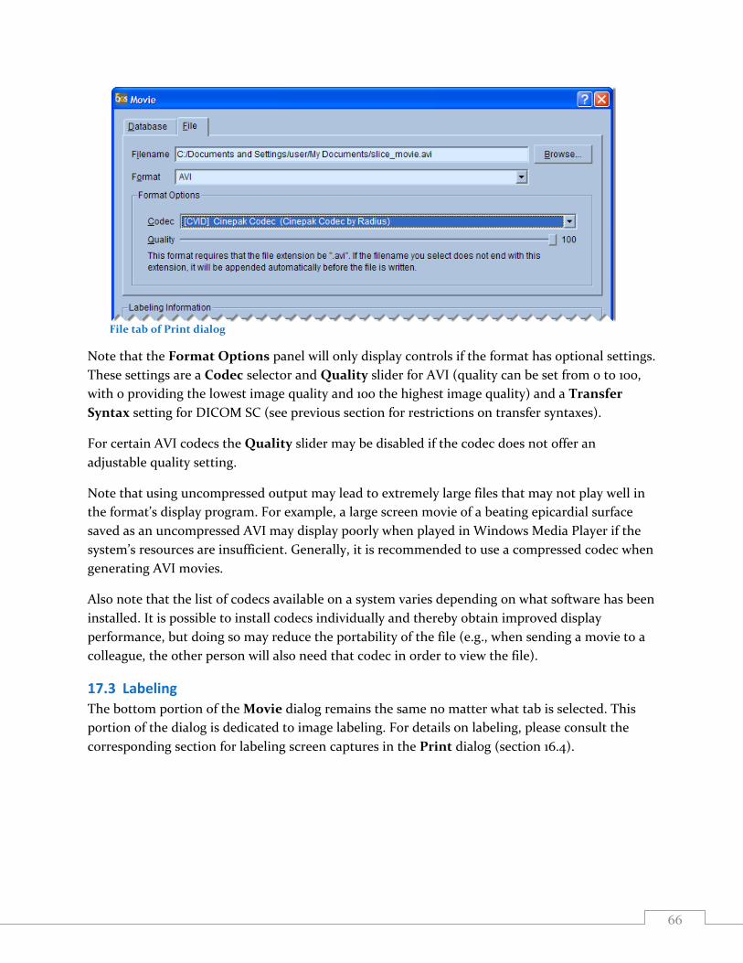
66
File tab of Print dialog
Note that the Format Options panel will only display controls if the format has optional settings.
These settings are a Codec selector and Quality slider for AVI (quality can be set from 0 to 100,
with 0 providing the lowest image quality and 100 the highest image quality) and a Transfer
Syntax setting for DICOM SC (see previous section for restrictions on transfer syntaxes).
For certain AVI codecs the Quality slider may be disabled if the codec does not offer an
adjustable quality setting.
Note that using uncompressed output may lead to extremely large files that may not play well in
the format’s display program. For example, a large screen movie of a beating epicardial surface
saved as an uncompressed AVI may display poorly when played in Windows Media Player if the
system’s resources are insufficient. Generally, it is recommended to use a compressed codec when
generating AVI movies.
Also note that the list of codecs available on a system varies depending on what software has been
installed. It is possible to install codecs individually and thereby obtain improved display
performance, but doing so may reduce the portability of the file (e.g., when sending a movie to a
colleague, the other person will also need that codec in order to view the file).
17.3 Labeling
The bottom portion of the Movie dialog remains the same no matter what tab is selected. This
portion of the dialog is dedicated to image labeling. For details on labeling, please consult the
corresponding section for labeling screen captures in the Print dialog (section 16.4).
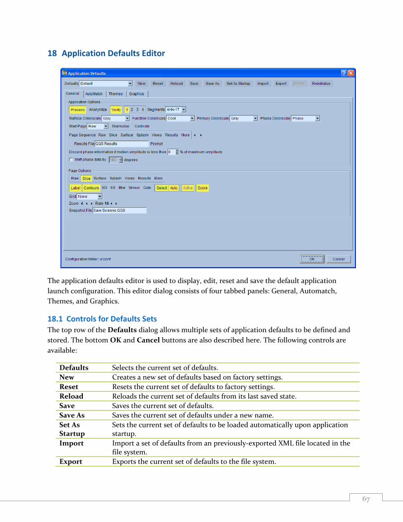
67
18 Application Defaults Editor
The application defaults editor is used to display, edit, reset and save the default application
launch configuration. This editor dialog consists of four tabbed panels: General, Automatch,
Themes, and Graphics.
18.1 Controls for Defaults Sets
The top row of the Defaults dialog allows multiple sets of application defaults to be defined and
stored. The bottom OK and Cancel buttons are also described here. The following controls are
available:
Defaults Selects the current set of defaults.
New Creates a new set of defaults based on factory settings.
Reset Resets the current set of defaults to factory settings.
Reload Reloads the current set of defaults from its last saved state.
Save Saves the current set of defaults.
Save As Saves the current set of defaults under a new name.
Set As Startup
Sets the current set of defaults to be loaded automatically upon application startup.
Import Import a set of defaults from an previously-exported XML file located in the file system.
Export Exports the current set of defaults to the file system.

68
Delete Deletes the current set of defaults. Not available for None, Default, or Factory defaults.
Reinitialize Resets the Default set of defaults to its factory settings and make this set the startup set of defaults
OK Applies current defaults to the application (one-time).
Cancel Exits default dialog without making any changes.
Defaults can be selected on the fly from the main application window by selecting a set from the
Defaults drop-down list.
18.2 General Settings
The general panel is divided into two sections: one for application wide settings and one for page
specific settings. The application settings are:
Process Toggles automatic processing of input datasets.
PFQ Enables PFQ normal limits databases. If this is disabled, perfusion defects are calculated using the old normal limits method.
Anonymize Toggles off display of patient identification.
1 2 3 4 Sets default display mode (one, two, three or four datasets).
Score Sets display of scoring polar maps.
Report Sets the initial state of the ARG (Auto Report Generator) panel.
Segments Sets the default scoring model to Cedars 20-segment or AHA 17-segment.
Convert Converts old ARG studies from 20 segments to 17 segments (if applicable). If unchecked, old ARG studies will load in the number of segments they were saved with.
Surface Color scale
Sets the default surface color scale for all 3D surface images.
Function Color scale
Sets the default polar map / parametric surface color scale.
Primary Color scale
Sets the default color scale for all 2D images.
Normalize Toggles automatic normalization of display windowing levels based on segmented LV surfaces or regions.
Sequence Defines default page ordering on the toolbar.
Normal Limits Sets default perfusion normal limits.
Browse Allows selection of default normal limits.
Results File Sets results file dataset ID.
Prompt Toggles prompting for a file name when saving results.
The following settings are available on the General tab page in the Page Options section:
Availability of any setting is specific to the page selected in this section.
Label Toggles image labeling.
Lines Toggles motion reference lines.
Spin Toggles continuous spatial cine.
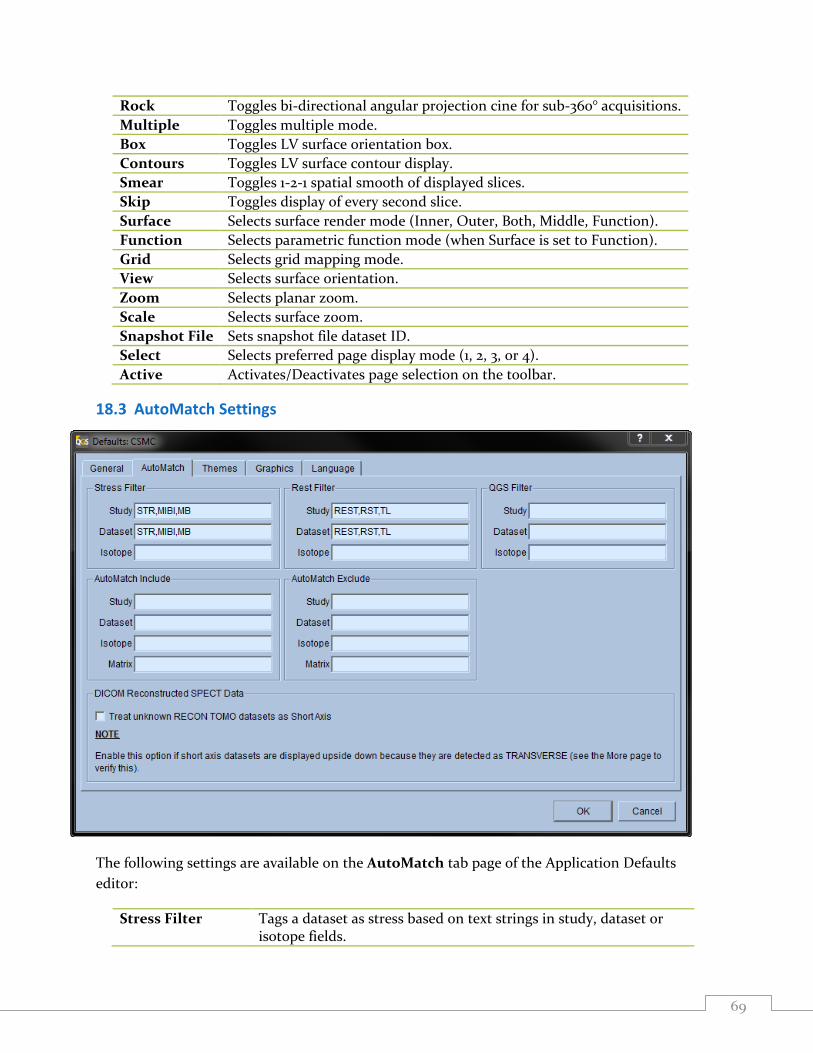
69
Rock Toggles bi-directional angular projection cine for sub-360° acquisitions.
Multiple Toggles multiple mode.
Box Toggles LV surface orientation box.
Contours Toggles LV surface contour display.
Smear Toggles 1-2-1 spatial smooth of displayed slices.
Skip Toggles display of every second slice.
Surface Selects surface render mode (Inner, Outer, Both, Middle, Function).
Function Selects parametric function mode (when Surface is set to Function).
Grid Selects grid mapping mode.
View Selects surface orientation.
Zoom Selects planar zoom.
Scale Selects surface zoom.
Snapshot File Sets snapshot file dataset ID.
Select Selects preferred page display mode (1, 2, 3, or 4).
Active Activates/Deactivates page selection on the toolbar.
18.3 AutoMatch Settings
The following settings are available on the AutoMatch tab page of the Application Defaults
editor:
Stress Filter Tags a dataset as stress based on text strings in study, dataset or isotope fields.
70
Rest Filter Tags a dataset as rest based on text strings in study, dataset or isotope fields.
AutoMatch Include
Tags a dataset as active based on text strings in study, dataset, isotope or matrix fields. In the Dataset Editor, active datasets are highlighted in yellow.
AutoMatch Exclude
Tags a dataset as inactive based on text strings in study, dataset, isotope or matrix fields. In the Dataset Editor, inactive datasets are not highlighted.
DICOM Reconstructed SPECT Data
When enabled, the application will assume that DICOM datasets that are of RECON TOMO or GATED RECON TOMO image type but contain no view type are short axis datasets
The following actions are supported:
OK Applies AutoMatch settings for the current QPS processing session and closes the Application Defaults screen. Settings are not saved for future processing sessions.
Cancel Closes the Application Defaults screen without applying or saving changes.
Save Saves all AutoMatch settings to a file and are effective for every QPS session until changed and re-saved.
Reset Restores the AutoMatch defaults to the factory shipped settings.
Using Filters to Automatically Determine Dataset Category
Filters are used to automatically identify datasets as stress, rest, raw, short axis etc. A dataset is
identified by a Study name and a Dataset name. Carefully selecting filters to identify datasets
allows the QPS application to run automatically and in a continuous manner without user
intervention. For example, if the QPS application is capable of determining which of all the
datasets selected are the stress and rest short axis datasets, then selection of normal limits and
generation of results is automatic. If QPS is unable to determine the stress and rest short axis
datasets, then results may not be calculated and the user must manually set the datasets using the
Dataset Selector pull-down menu.
Definitions used in this section:
Study: refers to the name of a dataset and typically identifies the dataset in general terms. For
example, a dataset with a study name of Rest Thallium suggests that the data is from either a rest
thallium acquisition or the data was generated from a processing procedure (raw data or
processed data, respectively).
Dataset: refers to the name of a dataset and typically identifies the dataset in more specific terms.
For example, a dataset name containing Raw or Short Axis suggests the dataset is raw data or
processed data, respectively.
When the two terms are use together, a dataset can be uniquely identified. A dataset with a Study
name of Rest Thallium and Dataset name of Short Axis identifies the dataset as a set of rest
thallium short axis tomographic slices.
71
The QPS application uses internal criteria to distinguish raw datasets from processed datasets and
then uses the AutoMatch filter settings to determine which processed datasets are to be used for
automatic processing. In particular, QPS needs to be able to identify a Primary stress and/or rest
short axis dataset. Typically, a study will contain a processed stress dataset and a processed rest
dataset but QPS will work if only one processed dataset is selected and used as input. If a study
contains more than two processed datasets (for example, processed stress, processed rest,
processed 24 hour delayed etc.), QPS will need a way to identify which two datasets are the
Primary stress/rest datasets.
The user has two methods to set the correct Primary stress/rest datasets.
1. Use the Dataset Editor and click the required Stress (or Rest) and Primary labels for the
datasets to highlight them (yellow Stress, yellow Primary).
2. Adjust the filter settings on the AutoMatch page of the Defaults Editor and let QPS
select (highlight) the correct datasets.
Using method 1), the user cannot select a Primary dataset unless the Stress and/or Rest label for
the dataset has also been selected. A further constraint is imposed (using either method) in that
QPS will not allow two Primary Stress datasets or two Primary Rest datasets, only one of each.
Note: Using the first method, the user cannot select a Primary dataset unless the Stress
and/or Rest label for the dataset has also been selected. A further constraint is imposed
(using either method) in that QPS will not allow two Primary Stress datasets or two
Primary Rest datasets, only one of each.
QPS, along with the AutoMatch filter criteria, uses a process of “pattern-matching” to match user
string entries in the Study and Dataset fields with the Study name and Dataset name to identify
stress datasets, rest datasets, a primary stress dataset and a primary rest dataset. Optionally,
isotope criteria may be entered in the Isotope field to further narrow down the identity of the
correct datasets.
The string entries may consist of complete names (e.g. Stress) or partial names (e.g. Str), numbers
(e.g. 24) and can include the wildcard characters question mark (?) and asterisk (*) for single and
multiple characters, respectively. A carat (^) can be used to match the beginning or the end of a
line. Multiple entries for the same field are permitted but must be separated by commas and not
have any spaces.
Examples using AutoMatch with filters
Example 1
In this first example, a patient named Test-1 will be used. All of the datasets for this patient will be
selected as input to the QPS application.
Selecting all the datasets for patient Test-1 and then clicking the QPS button will run the QPS
application with factory default settings for AutoMatch. Opening the Dataset Editor reveals the

72
default rest and stress datasets including primary datasets highlighted in yellow based on the
current AutoMatch settings. Using the factory shipped filter settings, the STR MIBI Prone short
axis dataset (Stress SAX) is automatically selected as the Primary stress dataset by QPS. Normally,
the STR MIBI Supine short axis dataset (Stress SAX) would be used as the Primary stress dataset.
As mentioned previously, the user can use the Dataset Editor to manually select the correct
Stress/Rest Primary datasets. However, careful setting of filter parameters on the AutoMatch
page requires no manual intervention by the user. In this example, the user could type Supine (or
Sup, or sup etc.) in the Study field of the Primary Stress Filter, click OK or Save to automatically
set the Primary Stress dataset.
Setting AutoMatch filters for the first time is probably done best by clearing the existing factory
shipped settings and then trying the most common combinations of Study name and Dataset
name for the user’s site naming conventions.
Dataset Editor Window
For the datasets used in this example, filter settings shown could be used as default settings if the
naming conventions were consistent among patient studies. Looking at the Dataset Editor one
can see that all datasets have been correctly defined as Stress or Rest and that the correct Primary
datasets have been identified. These filter settings will be saved by clicking OK and used in the
next example where the dataset naming convention is different.

73
AutoMatch settings, Example 1
Dataset Editor using filter settings above
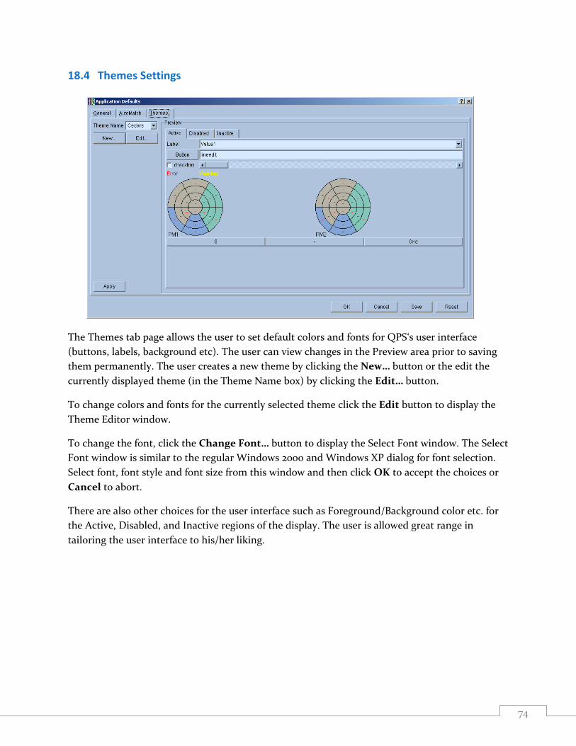
74
18.4 Themes Settings
The Themes tab page allows the user to set default colors and fonts for QPS‘s user interface
(buttons, labels, background etc). The user can view changes in the Preview area prior to saving
them permanently. The user creates a new theme by clicking the New… button or the edit the
currently displayed theme (in the Theme Name box) by clicking the Edit… button.
To change colors and fonts for the currently selected theme click the Edit button to display the
Theme Editor window.
To change the font, click the Change Font… button to display the Select Font window. The Select
Font window is similar to the regular Windows 2000 and Windows XP dialog for font selection.
Select font, font style and font size from this window and then click OK to accept the choices or
Cancel to abort.
There are also other choices for the user interface such as Foreground/Background color etc. for
the Active, Disabled, and Inactive regions of the display. The user is allowed great range in
tailoring the user interface to his/her liking.
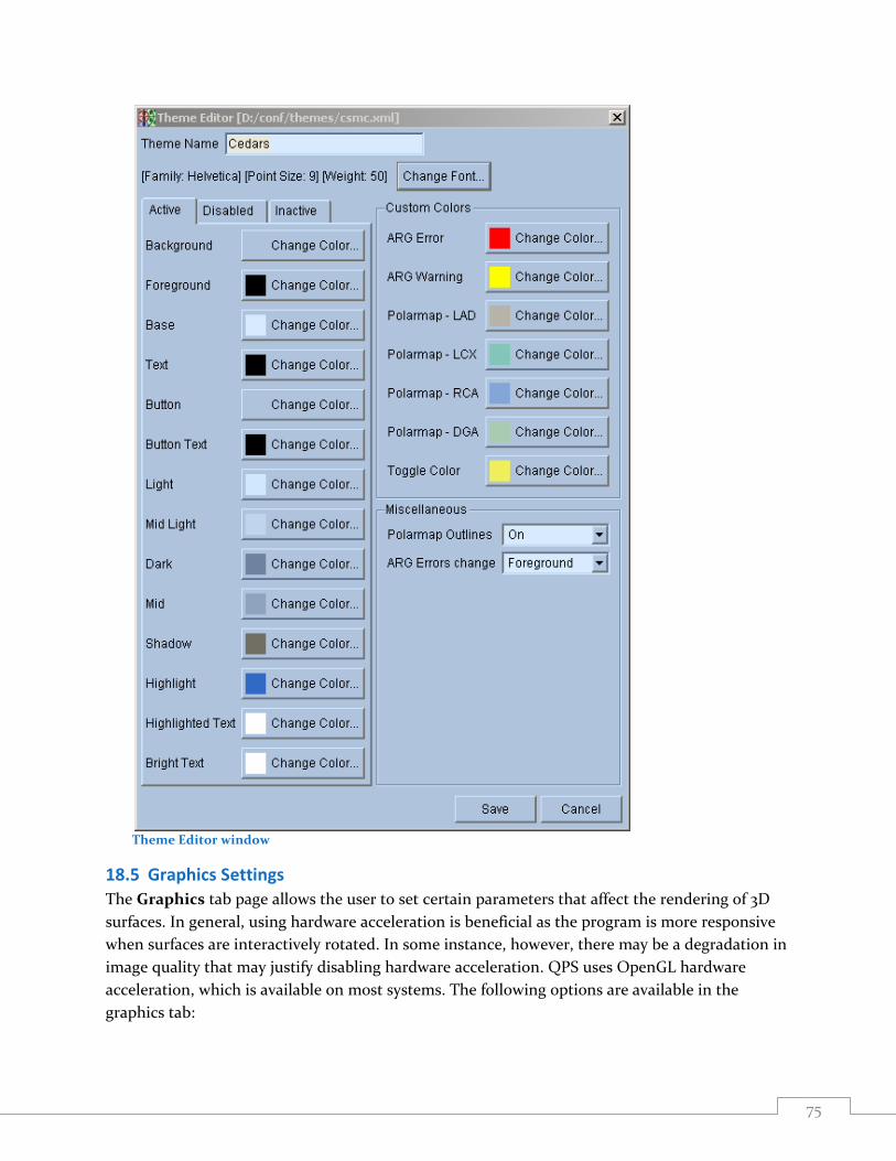
75
Theme Editor window
18.5 Graphics Settings
The Graphics tab page allows the user to set certain parameters that affect the rendering of 3D
surfaces. In general, using hardware acceleration is beneficial as the program is more responsive
when surfaces are interactively rotated. In some instance, however, there may be a degradation in
image quality that may justify disabling hardware acceleration. QPS uses OpenGL hardware
acceleration, which is available on most systems. The following options are available in the
graphics tab:

76
Enable 3D OpenGL hardware rendering
If hardware rendering causes problems, it may be necessary to disable OpenGL by unchecking this checkbox. Turning off this option may adversely affect performance for some advanced visualization tasks such as viewing coronary trees. In case of issues with rendering, try turning off hardware acceleration first (see below). Note: changing this setting will only affect viewports that have not been created yet, i.e., to pages that have not been visited. To apply this setting fully, save the defaults and restart the application.
Enable OpenGL hardware acceleration
If hardware acceleration causes problems, it is recommended to disable OpenGL hardware acceleration by setting this option to No. A typical issue involves dual monitor setups where on the secondary display the 3D viewports appear “frozen.” If this is the case, set acceleration to No, save the defaults and restart the application. Note: changing this setting will only affect viewports that have not been created yet, i.e., to pages that have not been visited. To apply this setting fully, save the defaults and restart the application.
Enable specular highlights
If OpenGL is enabled, surfaces can be rendered with added specular reflections. This adds a “shiny” appearance to the surfaces, potentially making it easier to visually assess the shape of the surface. This can be useful for isosurfaces, but may also be distracting. If checked, the amount of specular reflection can be controlled using the Surface shininess slider.
Surface shininess
Controls the amount of specular reflection (or “shine”), from 0 (none) to 100 (maximum reflection).
Enable parametric image shading
If enabled, parametrically-mapped surfaces (such as perfusion-, Fourier phase- and amplitude-mapped surfaces) are also shaded. In some cases, the shading may interfere with the interpretation of the parametric mapping, hence the ability to disable this option.
Graphics tab
77
Hardware rendering and acceleration
The Notes in the graphics tab help describe the OpenGL hardware rendering options. The
viewport with the cube at the bottom left of the tab is active and can be used to determine what
functionality is available on multiple monitors by dragging the Defaults dialog to another screen,
then attempting to rotate the cube by left-dragging with the mouse. If the rotation succeeds,
hardware acceleration is supported on that monitor. If the viewport appears frozen, hardware
acceleration is not supported and should be disabled for this system, which will allow OpenGL
viewport to function correctly on all monitors, trading rendering performance for compatibility.
It is also possible to use a configuration file to let the system decide whether to enable hardware
acceleration or not “automatically.” Acceleration will be enabled by default if the setting is set to
Auto, unless the identifier of the graphics card is found in a “blacklist” file named opengl.xml
and located in the system’s configuration folder for CSMC software (listed at the bottom of the
Defaults dialog after Configuration folder). The contents of this XML file look as follows:
<!DOCTYPE OpenGLRendererBlackList>
<OpenGLRendererBlackList>
<Renderer Id="Implementation_String_1" />
<Renderer Id="Implementation_String_2" />
...
<Renderer Id="Implementation_String_n" />
</OpenGLRendererBlackList>
Where the line containing “Implementation_String_x” may be repeated for a variety of graphics
adapters. A complete line can be obtained by clicking Copy to Clipboard in the Graphics tab.
For the adapter in the graphics tab example above, the line with the implementation string should
read
<Renderer Id="NVIDIA Corporation: GeForce 8800 GTS/PCI/SSE2" />
If the setting is Yes, hardware acceleration will be enabled whether the adapter’s identification
string is found in the blacklist file or not. This can be used for testing without requiring changes
to the blacklist file.
Highlights and shading
The following figures show examples of parametrically-mapped perfusion surfaces with various
settings for the graphics options.
NOTE: specular reflection and shading should be taken into account if parametric surfaces are
evaluated. If such surfaces are used to assess the patient’s condition, it is recommended to turn off
parametric shading and specular reflections.

78
Hardware acceleration, no parametric shading or specular reflections
Hardware acceleration, parametric shading enabled
Hardware acceleration, parametric shading and specular reflections enabled
No hardware acceleration, parametric shading, or specular reflections
No hardware acceleration, parametric shading enabled, no specular reflections
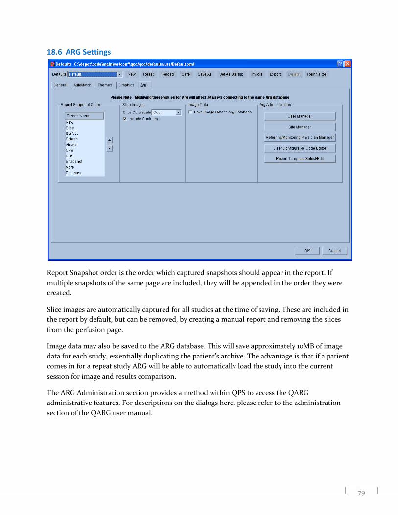
79
18.6 ARG Settings
Report Snapshot order is the order which captured snapshots should appear in the report. If
multiple snapshots of the same page are included, they will be appended in the order they were
created.
Slice images are automatically captured for all studies at the time of saving. These are included in
the report by default, but can be removed, by creating a manual report and removing the slices
from the perfusion page.
Image data may also be saved to the ARG database. This will save approximately 10MB of image
data for each study, essentially duplicating the patient’s archive. The advantage is that if a patient
comes in for a repeat study ARG will be able to automatically load the study into the current
session for image and results comparison.
The ARG Administration section provides a method within QPS to access the QARG
administrative features. For descriptions on the dialogs here, please refer to the administration
section of the QARG user manual.
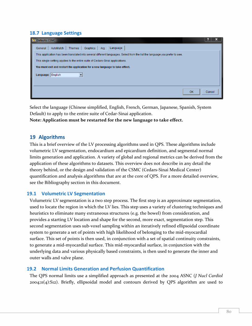
80
18.7 Language Settings
Select the language (Chinese simplified, English, French, German, Japanese, Spanish, System
Default) to apply to the entire suite of Cedar-Sinai application.
Note: Application must be restarted for the new language to take effect.
19 Algorithms This is a brief overview of the LV processing algorithms used in QPS. These algorithms include
volumetric LV segmentation, endocardium and epicardium definition, and segmental normal
limits generation and application. A variety of global and regional metrics can be derived from the
application of these algorithms to datasets. This overview does not describe in any detail the
theory behind, or the design and validation of the CSMC (Cedars-Sinai Medical Center)
quantification and analysis algorithms that are at the core of QPS. For a more detailed overview,
see the Bibliography section in this document.
19.1 Volumetric LV Segmentation
Volumetric LV segmentation is a two step process. The first step is an approximate segmentation,
used to locate the region in which the LV lies. This step uses a variety of clustering techniques and
heuristics to eliminate many extraneous structures (e.g. the bowel) from consideration, and
provides a starting LV location and shape for the second, more exact, segmentation step. This
second segmentation uses sub-voxel sampling within an iteratively refined ellipsoidal coordinate
system to generate a set of points with high likelihood of belonging to the mid-myocardial
surface. This set of points is then used, in conjunction with a set of spatial continuity constraints,
to generate a mid-myocardial surface. This mid-myocardial surface, in conjunction with the
underlying data and various physically based constraints, is then used to generate the inner and
outer walls and valve plane.
19.2 Normal Limits Generation and Perfusion Quantification
The QPS normal limits use a simplified approach as presented at the 2004 ASNC (J Nucl Cardiol
2004;11(4):S12). Briefly, ellipsoidal model and contours derived by QPS algorithm are used to
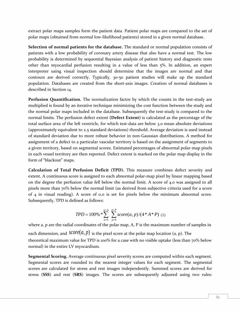
81
extract polar maps samples form the patient data. Patient polar maps are compared to the set of
polar maps (obtained from normal low-likelihood patients) stored in a given normal database.
Selection of normal patients for the database. The standard or normal population consists of
patients with a low probability of coronary artery disease that also have a normal test. The low
probability is determined by sequential Bayesian analysis of patient history and diagnostic tests
other than myocardial perfusion resulting in a value of less than 5%. In addition, an expert
interpreter using visual inspection should determine that the images are normal and that
contours are derived correctly. Typically, 30-50 patient studies will make up the standard
population. Databases are created from the short-axis images. Creation of normal databases is
described in Section 14.
Perfusion Quantification. The normalization factor by which the counts in the test-study are
multiplied is found by an iterative technique minimizing the cost function between the study and
the normal polar maps included in the database. Subsequently the test-study is compared to the
normal limits. The perfusion defect extent (Defect Extent) is calculated as the percentage of the
total surface area of the left ventricle, for which test-data are below 3.0 mean absolute deviations
(approximately equivalent to 2.5 standard deviations) threshold. Average deviation is used instead
of standard deviation due to more robust behavior in non-Gaussian distributions. A method for
assignment of a defect to a particular vascular territory is based on the assignment of segments to
a given territory, based on segmental scores. Estimated percentages of abnormal polar-map pixels
in each vessel territory are then reported. Defect extent is marked on the polar map display in the
form of “blackout” maps.
Calculation of Total Perfusion Deficit (TPD). This measure combines defect severity and
extent. A continuous score is assigned to each abnormal polar-map pixel by linear mapping based
on the degree the perfusion value fell below the normal limit. A score of 4.0 was assigned to all
pixels more than 70% below the normal limit (as derived from subjective criteria used for a score
of 4 in visual reading). A score of 0.0 is set for pixels below the minimum abnormal score.
Subsequently, TPD is defined as follows:
0 0
100%* ( , ) /(4* * )p Pa A
a p
TPD score a p A P
(1)
where a, p are the radial coordinates of the polar map, A, P is the maximum number of samples in
each dimension, and ( , )score a p is the pixel score at the polar map location (a, p). The
theoretical maximum value for TPD is 100% for a case with no visible uptake (less than 70% below
normal) in the entire LV myocardium.
Segmental Scoring. Average continuous pixel severity scores are computed within each segment.
Segmental scores are rounded to the nearest integer values for each segment. The segmental
scores are calculated for stress and rest images independently. Summed scores are derived for
stress (SSS) and rest (SRS) images. The scores are subsequently adjusted using two rules:
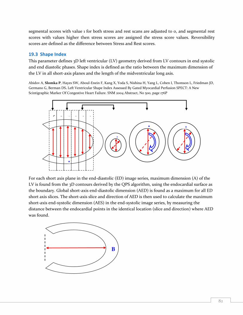
82
segmental scores with value 1 for both stress and rest scans are adjusted to 0, and segmental rest
scores with values higher then stress scores are assigned the stress score values. Reversibility
scores are defined as the difference between Stress and Rest scores.
19.3 Shape Index
This parameter defines 3D left ventricular (LV) geometry derived from LV contours in end systolic
and end diastolic phases. Shape index is defined as the ratio between the maximum dimension of
the LV in all short-axis planes and the length of the midventricular long axis.
Abidov A, Slomka P, Hayes SW, Aboul-Enein F, Kang X, Yoda S, Nishina H, Yang L, Cohen I, Thomson L, Friedman JD,
Germano G, Berman DS. Left Ventricular Shape Index Assessed By Gated Myocardial Perfusion SPECT: A New
Scintigraphic Marker Of Congestive Heart Failure. SNM 2004 Abstract, No 500, page 176P
For each short axis plane in the end-diastolic (ED) image series, maximum dimension (A) of the
LV is found from the 3D contours derived by the QPS algorithm, using the endocardial surface as
the boundary. Global short-axis end-diastolic dimension (AED) is found as a maximum for all ED
short axis slices. The short-axis slice and direction of AED is then used to calculate the maximum
short-axis end-systolic dimension (AES) in the end-systolic image series, by measuring the
distance between the endocardial points in the identical location (slice and direction) where AED
was found.
B
A
1 2 3 4 5 6
A
A
A

83
The long-axis dimension of the myocardium is derived by calculating the distance (B) between
the most apical point on the endocardial surface and the center of the valve plane. The ED long-
axis dimension (BED) is calculated independently from the ES long-axis dimension (BES).
The end-diastolic shape index (SI ED) and the end-systolic shape index (SI ES) are derived by
AED/BED and AES/BES, respectively.
19.4 Eccentricity
Eccentricity is a measure of the elongation of the LV, and varies from 0 (sphere) to 1 (line); it is calculated from the
major axis RZ and the minor axes RX and RY of the ellipsoid that best fits the mid-myocardial surface, according to
the formula:
√
It is calculated for all slices in a gated series.
19.5 Global Functions
The following standard global functions are computed:
Volume The LV chamber volume in ml.
Area The mid-myocardial surface area in cm2.
19.6 Regional Function
The regional functions are computed by generating parametric surfaces within the canonical LV
coordinate system.
The perfusion parametric surface is generated by assigning to each point on the mid-myocardial
surface the maximum end-diastolic counts along the count profile normal to that point and lying
between the inner and outer myocardial surfaces.
RX RZ
RY
84
20 References 1. Germano G, Kiat H, Kavanagh PB, Moriel M, Mazzanti M, Su HT, Van Train KF, Berman
DS. Automatic quantification of ejection fraction from gated myocardial perfusion SPECT.
J Nucl Med 1995;36(11):2138-47.
2. Germano G, Erel J, Lewin H, Kavanagh PB, Berman DS. Automatic quantitation of regional
myocardial wall motion and thickening from gated technetium-99m sestamibi myocardial
perfusion single-photon emission computed tomography. J Am Coll Cardiol
1997;30(5):1360-7.
3. Berman D, Germano G. An approach to the interpretation and reporting of gated
myocardial perfusion SPECT. In: G Germano and D Berman, eds. Clinical gated cardiac
SPECT. Futura Publishing Company, Armonk; 1999:147-182.
4. Germano G, Berman D. Quantitative gated perfusion SPECT. In: G Germano and D
Berman, eds. Clinical gated cardiac SPECT. Futura Publishing Company, Armonk;
1999:115-146.
5. Sharir T, Germano G, Kavanagh P, Lai S, Cohen I, Lewin H, Friedman J, Zellweger M,
Berman D. Incremental prognostic value of post-stress left ventricular ejection fraction
and volume by gated myocardial perfusion single photon emission computed tomography.
Circulation 1999;100(10):1035-1042.
6. Berman D.S., Kang X.P., Abidov A., Cohen I., Hayes S.W., Friedman J.D., Sciammarella M.,
German G., Aboul-Enein F., Hachamovitch R., Prognostic value of myocardial perfusion
SPECT comparing 17-segment and 20-segment scoring systems. J Am Coll Cardiology,
2003 (abstract). 41(6(Suppl.A)):p. 445A.
7. Slomka, PJ; Nishina, H; Berman, DS; Kang, X; Akincioglu, C; Friedman, JD; Hayes, SW;
Aladl, UE; Germano, G; “Motion-Frozen” Display and Quantification of Myocardial
Perfusion. J Nucl Med 2004;45(7):1128-1134.