Quaderni del Dipartimento di Matematica

Universita degli Studi di Parma

Elio Panegai and Gianfranco Rossi1 (Eds.)

Proceedings of CILC’04Italian Conference on Computational Logic

November 16, 2004 n. 390

1Dipartimento di Matematica, Universita di Parma, I-43100 Parma, Italy,gianfr@prmat.math.unipr.it

Gianfranco Rossi Elio Panegai (Eds.)

CILC’04ITALIAN CONFERENCE ON COMPUTATIONAL LOGIC

Nineteenth Annual Meeting of GULP - (Associazione Italiana Gruppo Ricer-catori e Utenti di Logic Programming)

June 16-17, 2004Parma, Italy

PROCEEDINGS

Preface

This report contains the Proceedings of the CILC’04 Italian Conference on Computa-tional Logic held in Parma (Italy), June 16-17, 2004. This is the 19th annual meeting ofthe Italian Association “Gruppo Ricercatori e Utenti di Logic Programming” (GULP).Previous GULP Conferences were held in Italy (from 1986 to 1993), and, since 1994,alternatively in Italy, Spain, Portugal (and Cuba, in 2000), in cooperation with theSpanish PRODE Association and the Portuguese Association for Artificial IntelligenceAPPIA. The 2004 edition changed its name to CILC in order to emphasize the Computa-tional Logic issue, and it moved again to a more “local” organization structure (anyway,still open to contributions from everywhere and with a wide scope of interests).

The technical program of the Conference includes 25 communications, organizedaccording to the following topics: Abductive Logic Programming, Automated Reason-ing, Constraints, Data Management, Learning and Knowledge Discovery, Logic-BasedAgents, Program Refinement and Transformation, Semantics. All papers have beenevaluated by two reviewers. In addition, the program includes an invited talk by LuısMoniz Pereira (U. Lisbon), three tutorials by Stefania Costantini (U. L’Aquila), AgostinoDovier (U. Udine) and Paolo Torroni (U. Bologna), and four “demo” presentations.

We wish to thanks all authors, the invited speaker, the tutorialists, the members ofthe Program Committee, all participants, and everyone who contributed to the successof the Conference.

Elio PanegaiJune 2004 Gianfranco Rossi

Editors

ii

Officials

Program Committee

Conference ChairmanGianfranco Rossi (Univ. di Parma)

Matteo Baldoni (Univ. di Torino)Francesco Buccafurri (Univ. ”Mediterranea” di Reggio Calabria)Michele Bugliesi (Univ. ”Ca Foscari” di Venezia)Marco Cadoli (Univ. ”La Sapienza” di Roma)Stefania Costantini (Univ. di L’Aquila)Giorgio Delzanno (Univ. di Genova)Agostino Dovier (Univ. di Udine)Andrea Formisano (Univ. di L’Aquila)Marco Gavanelli (Univ. di Ferrara)Fosca Giannotti (CNR, Pisa)Roberta Gori (Univ. di Pisa)Vincenzo Loia (Univ. di Salerno)Donato Malerba (Univ. di Bari)Maria Chiara Meo (Univ. ”G. d’Annunzio” di Chieti e Pescara)Andrea Omicini (Univ. di Bologna)Maurizio Proietti (IASI-CNR, Roma)Francesca Rossi (Univ. di Padova)Fausto Spoto (Univ. di Verona)Enea Zaffanella (Univ. di Parma)

Local Committee

Roberto Bagnara (Univ. di Parma)Dario Bianchi (Univ. di Parma)Elio Panegai (Univ. di Parma)Cristina Reggiani (Univ. di Parma)Gianfranco Rossi (Univ. di Parma)Enea Zaffanella (Univ. di Parma)

Organized by

GULP, Gruppo Ricercatori e Utenti di Logic Programming.

iii

With the contribution of:

Universita degli Studi di ParmaDipartimento di MatematicaCoLogNET

Contents

Invited Lecture

Revised Stable Models - a new semantics for logic programs . . . . . . . . . . . . . . . . . . . . . . . . . . . . . . . . . . . 3L. M. Pereira, A. M. Pinto

Tutorials

Answer Set Programming . . . . . . . . . . . . . . . . . . . . . . . . . . . . . . . . . . . . . . . . . . . . . . . . . . . . . . . . . . . . . . . . . . . . 7S. Costantini

Il problema del Protein Folding e i relativi approcci basati su programmazione con vincoli . . . . . . 8A. Dovier

Introduzione ai sistemi multi-agente basati su logica computazionale . . . . . . . . . . . . . . . . . . . . . . . . . . . 9P. Torroni

Contributed Talks

Abductive Logic Programming

Abduction with Hypotheses Confirmation . . . . . . . . . . . . . . . . . . . . . . . . . . . . . . . . . . . . . . . . . . . . . . . . . . . . 13M. Alberti, M. Gavanelli, E. Lamma, P. Mello, P. Torroni

Abductive Logic Programming with CIFF: Implementation and Applications . . . . . . . . . . . . . . . . . . 28U. Endriss, P. Mancarella, F. Sadri, G. Terreni, F. Toni

Automated Reasoning

A multi context-based Approximate Reasoning . . . . . . . . . . . . . . . . . . . . . . . . . . . . . . . . . . . . . . . . . . . . . . . 43L. Blandi, M. I. Sessa

A declarative approach to uncertainty orders . . . . . . . . . . . . . . . . . . . . . . . . . . . . . . . . . . . . . . . . . . . . . . . . 56A. Capotorti, A. Formisano

SAT-based Analysis of Cellular Automata . . . . . . . . . . . . . . . . . . . . . . . . . . . . . . . . . . . . . . . . . . . . . . . . . . . 73M. D’Antonio, G. Delzanno

Uniform relational frameworks for modal inferences . . . . . . . . . . . . . . . . . . . . . . . . . . . . . . . . . . . . . . . . . 88A. Formisano, E. G. Omodeo, E. S. Orlowska, A. Policriti

v

Constraints

Constraint Based Protein Structure Prediction Exploiting Secondary Structure . . . . . . . . . . . . . . 103R. Backofen, A. Dal Palu, A. Dovier, S. Will

Using a theorem prover for reasoning on constraint problems . . . . . . . . . . . . . . . . . . . . . . . . . . . . . . . 118M. Cadoli, T. Mancini

Constrained CP-nets . . . . . . . . . . . . . . . . . . . . . . . . . . . . . . . . . . . . . . . . . . . . . . . . . . . . . . . . . . . . . . . . . . . . . . 133S. Prestwich, F. Rossi, K. B. Venable, T. Walsh

Data Management

Efficient Evaluation of Disjunctive Datalog Queries with Aggregate Functions DB . . . . . . . . . . . 148M. Citrigno, W. Faber, G. Greco, N. Leone

Checking the Completeness of Ontologies: A Case Study from the Semantic Web . . . . . . . . . . . . 163V. Cordı, V. Mascardi

Combining logic programming and domain ontologies for text classification . . . . . . . . . . . . . . . . . . 178C. Cumbo, S. Iiritano, P. Rullo

Ontological encapsulation of many-valued logic . . . . . . . . . . . . . . . . . . . . . . . . . . . . . . . . . . . . . . . . . . . . . 189Z. Majkic

Learning and Knowledge Discovery

Frequent Pattern Queries for Flexible Knowledge Discovery . . . . . . . . . . . . . . . . . . . . . . . . . . . . . . . . . 202F. Bonchi, F. Giannotti, D. Pedreschi

Costruzione automatica di courseware in DyLOG (short paper) . . . . . . . . . . . . . . . . . . . . . . . . . . . . . . . 217L. Torasso

Improving efficiency of recursive theory learning . . . . . . . . . . . . . . . . . . . . . . . . . . . . . . . . . . . . . . . . . . . . 220A. Varlaro, M. Berardi, D. Malerba

Logic-Based Agents

From logic programs updates to action description updates . . . . . . . . . . . . . . . . . . . . . . . . . . . . . . . . . . 235J. Alferes, F. Banti, A. Brogi

Reasoning About Logic-based Agent Interaction Protocols . . . . . . . . . . . . . . . . . . . . . . . . . . . . . . . . . . . 250M. Baldoni, C. Baroglio, A. Martelli, V. Patti

Contracts in Multiagent Systems: the Legal Institution Perspective . . . . . . . . . . . . . . . . . . . . . . . . . . 265G. Boella, L. van der Torre

Integrating tuProlog into DCaseLP to Engineer Heterogeneous Agent Systems . . . . . . . . . . . . . . . 280I. Gungui, V. Mascardi

Communication Architecture in the DALI Logic Programming Agent-Oriented Language . . . . . 295S. Costantini, A. Tocchio, A. Verticchio

Programs Refinement and Trasformation

Preserving (Security) Properties under Action Refinement . . . . . . . . . . . . . . . . . . . . . . . . . . . . . . . . . . 310A. Bossi, C. Piazza, S. Rossi

Totally Correct Logic Program Transformations Using Well-Founded Annotations (short paper) 325A. Pettorossi, M. Proietti

Semantics

Implementing Joint Fixpoints Semantics on Top of DLV . . . . . . . . . . . . . . . . . . . . . . . . . . . . . . . . . . . 330F. Buccafurri, G. Caminiti

A compositional semantics for CHR . . . . . . . . . . . . . . . . . . . . . . . . . . . . . . . . . . . . . . . . . . . . . . . . . . . . . . . 345M. Gabbrielli, M. C. Meo

Demos

A demonstration of SOCS-SI . . . . . . . . . . . . . . . . . . . . . . . . . . . . . . . . . . . . . . . . . . . . . . . . . . . . . . . . . . . . . . 362M. Alberti, F. Chesani, M. Gavanelli, E. Lamma, P. Mello, P. Torroni

Constraint-based tools for protein folding . . . . . . . . . . . . . . . . . . . . . . . . . . . . . . . . . . . . . . . . . . . . . . . . . . . 365L. Bortolussi, A. Dal Palu, A. Dovier

The DALI Logic Programming Agent-Oriented Language . . . . . . . . . . . . . . . . . . . . . . . . . . . . . . . . . . . 368S. Costantini, A. Tocchio

The JSetL library: supporting declarative programming in Java . . . . . . . . . . . . . . . . . . . . . . . . . . . . . 372E. Panegai, E. Poleo, G. Rossi

Index of Authors

Invited Lecture

Revised Stable Models - a new semantics for logic programs

Luís Moniz Pereira and Alexandre Miguel Pinto

Centro de Inteligência Artificial, Universidade Nova de Lisboa 2829-516 Caparica, Portugal

lmp|amp@di.fct.unl.pt

Abstract This paper introduces an original 2-valued semantics for Normal Logic Programs (NLP), important on its own. Nevertheless, its name draws attention to that it is inspired by and generalizes Stable Model semantics (SM). The definitional distinction consists in the revision of one feature of SM, namely its treatment of odd loops over default negation. This single revised aspect, addressed by means of a Reductio ad Absurdum approach, affords us a fruitful cornucopia of consequences, namely regarding existence, relevance and top-down querying, cumulativity, and implementation. The paper motivates and then defines the Revised Stable Models semantics (rSM), justifying the definition and providing examples. It also presents two rSM semantics preserving program transformations into NLP without odd loops. Properties of rSM are given and contrasted with those of SM. Implementation is examined, and extensions of rSM are given with regard to explicit negation, ‘not’s in heads, and contradiction removal. Conclusions, further work, as well as potential use, terminate the paper. Keywords: Logic Program semantics, Stable Models, Reductio ad Absurdum.

Tutorials

Proposal of a Tutorial on Answer Set Programming

Stefania Costantini1

Dipartimento di Informatica,Universita degli Studi di L’Aquila,

L’Aquila, I-67100 Italy,stefcost@di.univaq.it

URL http://costantini.di.univaq.it

Abstract

Answer Set Programming (ASP) is an emerging paradigm of logic programming basedon the Answer Set (or equivalently Stable Model) semantics: each solution to a prob-lem is represented by an Answer Set (also called a Stable Model) of a deductivedatabase/function-free logic program encoding the problem itself. It is clearly relatedto deductive databases and knowledge bases, where the occurrence of several answersets indicates the presence of uncertain or incomplete knowledge, and each answer setrepresents a possible plausible instance of the database/knowledge base.

Recent work demonstrates that Answer Set Programming is a suitable paradigm fordefining and implementing data integration systems. In particular, the author of this pro-posal has defined a formalization in answer set programming, and a working inferenceengine, for the Global-as-View approach. The reason why answer set programming iswell suited for representing mapping s between data models is exactly that the query answering problem can be coped with also in the p resence of incomplete/ambiguous/inconsistent data sources: this by means of the advanced reasoning capabilities of com-putational logic, and by means of the possibility of making different plausible answers to queries explicit, as different answer set. The tutorial will introduce concepts and notions of computational logic, will describe the DATALOG¬ language and the answer set semantics, and will outline a comparison with traditional logic programming. However, the level of the description will be accessible to the non-expert, by providing few formal details intermixed with several intuitive examples. Some hints and references will be proposed for those who may wish to go into deeper detail.

Il Problema del Protein Folding e i Relativi Approcci Basati su Programmazione con Vincoli

1

Agostino Dovier Università degli Studi di Udine

Sommario

Le proteine sono presenti massivamente negli organismi viventi. Strutturalmente una pro-teina può essere considerata una catena costituita da elementi più semplici, detti aminoacidi.Gli aminoacidi possono essere di 20 tipi, mentre la lunghezza tipica di una proteina va da poche decine a diverse centinaia. Ogni proteina assume una determinata forma spaziale che ne caratterizza la funzione biologica. Oggigiorno è possibile scoprire la sequenza degli amminoacidi di una proteina, cosi come è possibile generare in laboratorio determinate sequenze di aminoacidi. Non esistono tuttavia ancora dei tools per predire la forma spaziale data la sequenza degli aminoacidi ne tantomeno delle tecniche di laboratorio che permettano di "fotografare" la forma spaziale di proteine esistenti in tempi ragionevoli. In questo tutorial si mostra come il constraint programming sia adatto ad affrontare il problema della predizione della forma spaziale di una proteina, la cui risoluzione ha ricadu-te immediate in medicina e nelle biotecnologie in generale.

Introduzione ai Sistemi Multi-Agente basati su Logica Computazionale

1

Paolo Torroni DEIS Bologna

Sommario

Negli ultimi anni c'è stata una notevole crescita di interesse verso un paradigma compu- tazionale noto sotto il nome di "sistemi multi-agente". Esso è l'oggetto di studio di una nuova area di ricerca che riunisce ed integra certi aspetti dell'Intelligenza Artificiale con altri tipici dei Sistemi Distribuiti, con l'idea di sviluppare modelli e architetture per agenti intelligenti. Questo breve tutorial vuole essere un'introduzione ai sistemi multi-agente intelli-genti, dal punto di vista dei modelli formali, e del ruolo importante che ha avuto e sta avendo la logica computazionale nell'affrontare problematiche di vario tipo, dalla rap-presentazione della conoscenza ai meccanismi di ragionamento, dalla semantica delle interazioni tra gli agenti ai modelli operazionali.

Contributed Talks

Abduction with Hypotheses Confirmation

Marco Alberti1, Marco Gavanelli1, Evelina Lamma1,Paola Mello2, and Paolo Torroni2

1 DI - University of Ferrara - Via Saragat, 1 - 44100 Ferrara, Italy.malberti|m gavanelli|elamma@ing.unife.it

2 DEIS - University of Bologna - Viale Risorgimento, 2 - 40136 Bologna, Italy.pmello|ptorroni@deis.unibo.it

Abstract. Abduction can be seen as the formal inference correspondingto human hypothesis making. It typically has the purpose of explain-ing some given observation. In classical abduction, hypotheses could bemade on events that may have occurred in the past. In general, abductivereasoning can be used to generate hypotheses about events possibly oc-curring in the future (forecasting), or may suggest further investigationsthat will confirm or disconfirm the hypotheses made in a previous step(as in scientific reasoning). We propose an operational framework basedon Abductive Logic Programming, which extends existing frameworksin many respects, including accommodating dynamic observations andhypothesis confirmation.

1 Introduction

Often, reasoning paradigms in artificial intelligence mimic human reasoning, pro-viding a formalization and a better understanding of the human basic inferences.Abductive reasoning can be seen as a formalization, in computational logics, ofhypotheses making. In order to explain observations, we hypothesize that some(unknown) events have happened, or that some (not directly measurable) prop-erties hold true. The hypothesized facts are then assumed as true, unless theyare disconfirmed in the following.

Hypothesis making is particularly important in scientific reasoning: scientistswill hypothesize properties about nature, which explain some observations; insubsequent work, they will try to prove (if possible), or at least to confirmthe hypotheses. This process leads often to generating new alternative sets ofhypotheses. Starting from hypotheses on the current situation, scientists try toforesee their possible consequences; this provides new hypotheses on the futurebehavior that will be confirmed or disconfirmed by the actual events.

A typical application of abductive reasoning is diagnosis. Starting from theobservation of symptoms, physicians hypothesize in general possible alternativediseases that may have caused them. Following an iterative process, they will tryto support their hypotheses, by prescribing further exams, of which they foreseethe possible alternative results. They will then drop the hypotheses disconfirmedby such results, and take as most faithful those supported by them. New findings,such as results of exams or new symptoms, may help generating new hypotheses.

We can then describe this kind of hypothetical reasoning process as composedby three main elements: classically, explaining observations, by assuming possible

causes of the observed effects; but also, adapting such assumptions to upcomingevents, such as new symptoms occurring, and foreseeing the occurrence of newevents, which may or may not occur indeed.

In Abductive Logic Programming, many formalisms have been proposed [1–6], along with proof procedures able to provide, given a knowledge base and someobservation, possible sets of hypotheses that explain the observation. IntegrityConstraints are used to drive the process of hypothesis generation, to make suchsets consistent, and possibly to suggest new hypotheses. Most frameworks focuson one aspect of abductive reasoning: assumption making, based on a staticknowledge and on some observation.

In this work, we extend the concepts of abduction and abductive proof pro-cedures in two main directions.

First, we cater for the dynamic acquisition of new facts (events), which possi-bly have an impact on the abductive reasoning process, and for confirmation (ordisconfirmation) of hypotheses based on such events. We propose a language,able to state required properties of the events supporting the hypotheses: forinstance, we could say that, given some combination of hypotheses and facts,we make the hypothesis that some new events will occur. We call this kind ofhypothesis expectation. For this purpose, we express expectations as abducibleliterals. Expectations can be “positive (to be confirmed by certain events occur-ring), or “negative” (to be confirmed by certain events not occurring).

Second, in our framework, we need to be able to state that some event isexpected to happen within some time interval: if the event does actually happenwithin it, the hypothesis is confirmed, it is disconfirmed otherwise. In doing so,we need to introduce variables (e.g. to model time), and to state constraints onvariables occurring in abducible atoms. Moreover, possible expectation could beinvolving universal quantification: this typically happens with negative expec-tations (“The patient is expected not to show symptom Q at all times”). Forthis reason, we also need to cater for abducibles possibly containing universallyquantified variables.

To summarize, the main new features of the present work with respect toclassical ALP frameworks are:

– dynamic update of the knowledge base to cater for new events, whose oc-currence interacts with the abductive reasoning process itself;

– confirmation and disconfirmation of hypotheses, by matching expectationsand actual events;

– hypotheses with universally quantified variables;– constraints a la Constraint Logic Programming [7].

We achieve these features by defining syntax, declarative and operational seman-tics of an abductive framework, based on an extension of the IFF proof procedure[4], called SCIFF[8].3 Being the SCIFF an extension of an existing abductive

3 Historically, the name SCIFF is due to the fact that this framework has been firstlyapplied to modelling protocol in agent Societies, and that is also deals with CLPConstraints.

2

framework, it also caters for classic abductive logic programming (static knowl-edge, no notion of confirmation by events). However, due to space limitations,in this work we only focus on the original new parts.

The SCIFF has been implemented using Constraint Handling Rules [9] andintegrated in a Java-based system for hypothetical reasoning [10].

In the following Sect. 2 we introduce our framework’s knowledge representa-tion. In Sect. 3 and 4 we provide declarative and operational semantics, and weshow a soundness result. In Sect. 5 we show an example of the functioning ofthe SCIFF in a multi-agent setting. Before concluding, we discuss about relatedwork in Sect. 6.

Additional details about the syntax of data structures used by the SCIFFand allowedness criteria used to prove soundness are given in [11].

2 Knowledge Representation

In this section we show the knowledge representation of the abstract abductiveframework of the SCIFF.

As typical abductive frameworks [12], ours is representated by a 3-tuple〈DKB, IC, A〉 where:

– DKB is the (dynamic) knowledge base, union of KB (a logic program,possibly containing abducibles in the body of the clauses, which does notchange during the computation) and HAP (the dynamic part, as explainedbelow);

– A is the set of abducible predicates (in our case, E, EN and their explicitnegations ¬E and ¬EN); and

– IC is the set of Integrity Constraints.

The set HAP is composed of ground facts (defining the H predicate), of theform

H(Description[,Time])

where Description is a ground term representing the event that happened andTime is an integer number representing the time at which the event happened.

The history HAP dynamically grows during the computation, as new eventshappen; we do not model here the source of such events, but it can be imaginedas a queue. We assume that events arrive in the same temporal order in whichthey happen.

The evolution of the history HAP reflects in the evolution of the abductiveframework, of which HAP is part. We can formalize the evolution as a sequenceDALP of frameworks, and denote with DALPHAP the specific instance associ-ated to a specific history HAP.

An instance DALPHAP of an abductive framework is queried with a goal G.The goal may contain both predicates defined in KB and abducibles.

The computation of an instance of an abductive framework will produce, byabduction, a set EXP of expectations, which represent events that are expectedto (but might not) happen (positive expectations, of the form E(Description[,Time]))

3

and events that are expected not to (but might) happen (negative expectations,of the form EN(Description[,Time])). Typically, expectations will contain vari-ables, over which CLP [7] constraints can be imposed.

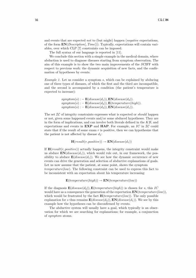
The full syntax of our language is reported in [11].We conclude this section with a simple example in the medical domain, where

abduction is used to diagnose diseases starting from symptom observation. Theaim of this example is to show the two main improvements of the SCIFF withrespect to previous work: the dynamic acquisition of new facts, and the confir-mation of hypotheses by events.

Example 1. Let us consider a symptom s, which can be explained by abducingone of three types of diseases, of which the first and the third are incompatible,and the second is accompanied by a condition (the patient’s temperature isexpected to increase):

symptom(s) : − E(disease(d1)),EN(disease(d3)).symptom(s) : − E(disease(d2)),E(temperature(high)).symptom(s) : − E(disease(d3)),EN(disease(d1)).

The set IC of integrity constraints expresses what is expected or should happenor not, given some happened events and/or some abduced hypotheses. They arein the form of implications, and can involve both literals defined in the KB, andexpectations and events in EXP and HAP. For example, an IC in IC couldstate that if the result of some exam r is positive, then we can hypothesize thatthe patient is not affected by disease d1:

H(result(r, positive)) → EN(disease(d1))

If H(result(r, positive)) actually happens, the integrity constraint would makeus abduce EN(disease(d1)), which would rule out, in our framework, the pos-sibility to abduce E(disease(d1)). We see how the dynamic occurrence of newevents can drive the generation and selection of abductive explanations of goals.Let us now assume that the patient, at some point, shows the symptomtemperature(low). The following constraint can be used to express this fact tobe inconsistent with an expectation about his temperature increasing:

E(temperature(high)) → EN(temperature(low))

If the diagnosis E(disease(d2)),E(temperature(high)) is chosen for s, this ICwould have as a consequence the generation of the expectation EN(temperature(low)),which would be frustrated by the fact H(temperature(low)). The only possibleexplanation for s thus remains E(disease(d3)),EN(disease(d1)). We see by thisexample how the hypotheses can be disconfirmed by events.

The abductive system will usually have a goal, which typically is an obser-vation for which we are searching for explanations; for example, a conjunctionof symptom atoms.

4

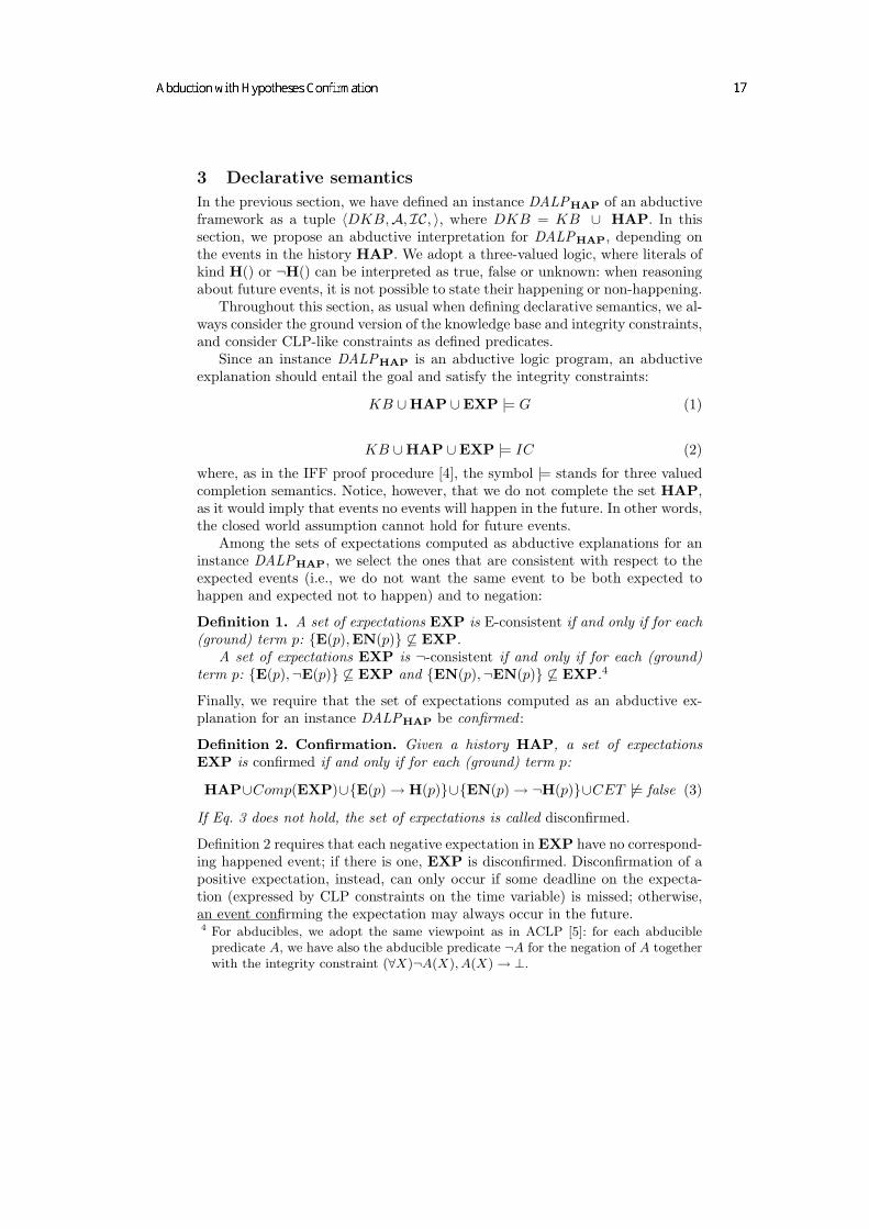
3 Declarative semantics

In the previous section, we have defined an instance DALPHAP of an abductiveframework as a tuple 〈DKB,A, IC, 〉, where DKB = KB ∪ HAP. In thissection, we propose an abductive interpretation for DALPHAP, depending onthe events in the history HAP. We adopt a three-valued logic, where literals ofkind H() or ¬H() can be interpreted as true, false or unknown: when reasoningabout future events, it is not possible to state their happening or non-happening.

Throughout this section, as usual when defining declarative semantics, we al-ways consider the ground version of the knowledge base and integrity constraints,and consider CLP-like constraints as defined predicates.

Since an instance DALPHAP is an abductive logic program, an abductiveexplanation should entail the goal and satisfy the integrity constraints:

KB ∪HAP ∪EXP |= G (1)

KB ∪HAP ∪EXP |= IC (2)

where, as in the IFF proof procedure [4], the symbol |= stands for three valuedcompletion semantics. Notice, however, that we do not complete the set HAP,as it would imply that events no events will happen in the future. In other words,the closed world assumption cannot hold for future events.

Among the sets of expectations computed as abductive explanations for aninstance DALPHAP, we select the ones that are consistent with respect to theexpected events (i.e., we do not want the same event to be both expected tohappen and expected not to happen) and to negation:

Definition 1. A set of expectations EXP is E-consistent if and only if for each(ground) term p: E(p),EN(p) 6⊆ EXP.

A set of expectations EXP is ¬-consistent if and only if for each (ground)term p: E(p),¬E(p) 6⊆ EXP and EN(p),¬EN(p) 6⊆ EXP.4

Finally, we require that the set of expectations computed as an abductive ex-planation for an instance DALPHAP be confirmed :

Definition 2. Confirmation. Given a history HAP, a set of expectationsEXP is confirmed if and only if for each (ground) term p:

HAP∪Comp(EXP)∪E(p) → H(p)∪EN(p) → ¬H(p)∪CET 6|= false (3)

If Eq. 3 does not hold, the set of expectations is called disconfirmed.

Definition 2 requires that each negative expectation in EXP have no correspond-ing happened event; if there is one, EXP is disconfirmed. Disconfirmation of apositive expectation, instead, can only occur if some deadline on the expecta-tion (expressed by CLP constraints on the time variable) is missed; otherwise,an event confirming the expectation may always occur in the future.4 For abducibles, we adopt the same viewpoint as in ACLP [5]: for each abducible

predicate A, we have also the abducible predicate ¬A for the negation of A togetherwith the integrity constraint (∀X)¬A(X), A(X) → ⊥.

5

4 Operational Semantics

Our framework’s IC are very much related to the integrity constraints of theIFF proof procedure [4]. This leads to the idea of using an extension of the IFFproof procedure for generating expectations, and check for their confirmation.

In particular, the additional features that we need are the following: (i) acceptnew events as they happen, (ii) produce a (disjunction of) set of expectations,(iii) detect confirmation of expectations, (iv) detect disconfirmation as soon aspossible.

The proof procedure that we are about to present is called SCIFF. FollowingFung and Kowalski’s approach [4], we describe the SCIFF as a transition system.Due to space limitations, we will only focus here on the new transitions, whilethe reader can refer to [4] for the basic IFF transitions.

4.1 Data StructuresThe SCIFF proof procedure is based on a transition system. Each state is definedby the tuple T ≡ 〈R, CS, PSIC,EXP,HAP,CONF,DISC〉, where R is theresolvent, CS is the constraint store, PSIC is the set of partially solved integrityconstraints, EXP is the set of (pending) expectations, HAP is the history ofhappened events, CONF is a set of confirmed hypotheses, DISC is a set ofdisconfirmed expectations.

Variable quantification In the IFF proof procedure, all the variables thatoccur in the resolvent or in abduced literals are existentially quantified, whilethe others (appearing only in implications) are universally quantified. Our proofprocedure has to deal with universally quantified variables in the abducibles andin the resolvent. In the IFF proof procedure, variables in an implication areexistentially quantified if they also appear in an abducible or in the resolvent.In our language, we can have existentially quantified variables in the integrityconstraints even if they do not occur elsewhere (see [11]).

For all these reasons, in the operational semantic specification we leave thevariable quantification explicit. Moreover, we need to distinguish between vari-ables that appear in abduced literals (or in the resolvent) and variables occurringonly in integrity constraints. The scope of the variables that occur only in animplication is the implication itself; the scope of the other variables is the wholetuple.

Initial Node and Success A derivation D is a sequence of nodes

T0 → T1 → . . . → Tn−1 → Tn.

Given a goal G and a set of integrity constraints IC, the first node is:

T0 ≡ 〈G, ∅, IC, ∅, ∅, ∅, ∅〉

i.e., the resolvent is initially the query (R0 = G) and the partially solvedintegrity constraints PSIC is the set of integrity constraints (PSIC0 = IC).

6

The other nodes Tj , j > 0, are obtained by applying the transitions defined inthe next section, until no transition can be applied anymore (quiescence). Everyarc in a derivation is labelled with the name of a transition.

Definition 3. Starting with an instance DALPHAPi there exists a successfulderivation for a goal G iff the proof tree with root node 〈G, ∅, IC, ∅,HAPi, ∅, ∅〉has at least one leaf node 〈∅, CS, PSIC,EXP,HAPf ,CONF, ∅〉 where HAPf ⊇HAPi and CS is consistent (i.e., there exists a ground variable assignment suchthat all the constraints are satisfied). In that case, we write:

DALPHAPi |∼HAPf

EXP∪CONF G

Notice that, coherently with the declarative semantics given earlier, a successnode cannot contain disconfirmed hypotheses. However, in some applications, allthe alternative sets may contain disconfirmed expectations and the goal couldbe finding a set of expectations with a minimal set of disconfirmed ones. Forthis reason, we preferred to map explicitly the set of disconfirmed expectations,instead of generating a simple fail node (paving the way for future extensions ofthe framework). Moreover, classical Logic Programming provides explanations(e.g., variable binding) about why a computation succeeds, but no explanationfor failure nodes. In our framework, a failure can be explained by means ofalternative sets of disconfirmed expectations.

From a non-failure leaf node N , answers can be extracted in a very similarway to the IFF proof procedure. First, a substitution σ′ is computed such that σ′

replaces all variables in N that are not universally quantified by ground terms,and σ′ satisfies all the constraints in the store CSN .

Definition 4. Let σ = σ′|vars(G) be the restriction of σ′ to the variables occur-ring in the initial goal G. Let ∆ = [CONFN ∪ EXPN )]σ′. The pair (∆,σ) isthe abductive answer obtained from the node N .

The SCIFF proof procedure performs some inferences based on the semanticsof time, under the temporal order assumption (see Sect. 2).

Consistency In order to ensure E-consistency of the set of expectations, werequire that the set IC of integrity constraints always contain the following:

E(T ) ∧EN(T ) → ⊥while for ¬-consistency, we impose the following integrity constraints:

E(T ) ∧ ¬E(T ) → ⊥ EN(T ) ∧ ¬EN(T ) → ⊥

4.2 TransitionsThe transitions are those of the IFF proof procedure, enlarged with those of CLP[7], and with specific transitions accommodating the concepts of confirmation ofhypotheses, and dynamically growing history.

7

In this section, the letter k will indicate the level of a node; each transitionwill generate one or more nodes from level k to k + 1. We will not explicitlyreport the new state for items that do not change; e.g., if a transition generatesa new node from the node

Tk ≡ 〈Rk, CSk, PSICk,EXPk,HAPk,CONFk,DISCk〉

and we do not explicitly state the value of Rk+1, it means that Rk+1 = Rk.

IFF-like transitions The SCIFF proof procedure contains transitions bor-rowed from the IFF proof procedure, namely Unfolding, Propagation, Splitting,Case Analysis, Factoring, Equivalence Rewriting and Logical Equivalence. Theyhave been extended to cope with abducibles containing universally quantifiedvariables and with CLP constraints. We omit them here for lack of space; thebasic transitions were proposed by Fung and Kowalski [4], while the extendedones can be found in a technical report [13].

Dynamically growing history The happening of events is dealt with by atransition Happening. This transition takes an event H(Event) from the externalqueue and puts it in the history HAP; the transition Happening is applicableonly if an Event such that H(Event) 6∈ HAP is in the external queue.

Formally, from a node Nk transition Happening produces a single successor

HAPk+1 = HAPk ∪ H(Event).

Note that transition Happening should be applied to all the non-failure nodes(in the frontier).

Confirmation and Disconfirmation

Disconfirmation EN Given a node N with the following situation:

EXPk = EXP′ ∪ EN(E1) HAPk = HAP′ ∪ H(E2)

Disconfirmation EN produces two nodes N1 and N2, as follows:

N1 N2

EXP1k+1 = EXP′ EXP2

k+1 = EXPk

DISC1k+1 = DISCk ∪ EN(E1) DISC2

k+1 = DISCk

CS1k+1 = CSk ∪ E1 = E2 CS2

k+1 = CSk ∪ E1 6= E2

Remember that node N1 is a failure node, as in success nodes DISC = ∅ (seeSect. 3).

Example 2. Suppose that HAPk = H(p(1, 2)) and ∃X∀Y EXPk = EN(p(X,Y )).Disconfirmation EN will produce the two following nodes:

8

∃X∀Y EXPk = EN(p(X,Y )) HAPk = H(p(1, 2))

CS1k+1 = X = 1 ∧ Y = 2 CS2

k+1 = X 6= 1 ∨ Y 6= 2DISC1

k+1 = EN(p(1, 2))CSk+2 = X 6= 1

where the last simplification in the right branch is due to the rules of the con-straint solver (see Section CLP).

Confirmation E Starting from a node N as follows:

EXPk = EXP′ ∪ E(E1), HAPk = HAP′ ∪ H(E2)

Confirmation E builds two nodes, N1 and N2; in node N1 we assume that theexpectation and the happened event unify, and in node N2 we hypothesize thatthe two do not unify:

N1 N2

EXP1k+1 = EXP′ EXP2

k+1 = EXPk

CONF1k+1 = CONFk ∪ E(E1) CONF2

k+1 = CONFk

CS1k+1 = CSk ∪ E1 = E2 CS2

k+1 = CSk ∪ E1 6= E2

In this case, N2 is not a failure node, as E(E1) might be confirmed by otherevents.

Disconfirmation E In order to check the disconfirmation of a positive expectationE, we need to assume that there will never be a matching event in the externalqueue. We can, e.g., exploit the semantics of time. If we make the hypothesis oftemporal ordering (Sect. 2), we can infer that an expected event for which thedeadline is passed, is disconfirmed.

Given a node:

– EXPk = E(X,T ) ∪EXP′

– HAPk = H(Y, Tc) ∪HAP′

– ∀E2, T2 : H(E2, T2) ∈ HAPk, CSk ∪ (E2, T2) = (X, T ) |= ⊥– CSk |= T < Tc

transition Disconfirmation E is applicable and creates the following node:

– EXPk+1 = EXP′

– DISCk+1 = DISCk ∪ E(X, T ).Operationally, one can often avoid checking that (X, T ) does not unify with everyevent in the history by choosing a preferred order of application of the transitions.By applying Disconfirmation E only if no other transition is applicable, thecheck can be safely avoided, as the test of confirmation is already performed byConfirmation E.

Notice that this transition infers the current time from happened event; i.e.,it infers that the current time cannot be less than the time of a happened event.

9

Symmetrically to Disconfirmation E, we also have a transition ConfirmationEN, which we do not report here for lack of space; the interested reader isreferred to [13].

Note that the entailment of constraints from a constraint store is, in general,not easy to verify. In the particular case of CSk |= T < Tc, however, we havethat the constraint T < Tc is unary (Tc is always ground), thus a CLP for finitedomains solver CLP(FD) is able to verify the entailment very easily if the storecontains only unary constraints (it is enough to check the maximum value inthe domain of T ). Moreover, even if the store contains non-unary constraints(thus the solver performs, in general, incomplete propagation), the transitionwill not compromise the soundness and completeness of the proof procedure. Ifthe solver performs a powerful propagation (including pruning, in CLP(FD)),the disconfirmation will be early detected, otherwise, it will be detected lateron.

CLP Here we adopt the same transitions as in CLP [7]. Therefore, the symbols= and 6= are in the constraint language. Note that a constraint solver workson a constraint domain which has an associated interpretation. In addition, theconstraint solver should handle the constraints among terms derived from theunification. Therefore, beside the specific constraint propagation on the con-straint domain, we need further inference rules for coping with the unification.For space limitations, we cannot show them here: but they can be found in [11].

4.3 SoundnessThe following proposition relates the operational notion of successful derivationwith the corresponding declarative notion of goal provability.

Proposition 1. Given an instance ALPHAPi of an ALP program and a groundgoal G, if DALPHAPi |∼HAPf

EXP∪CONF G then DALPHAPf |≈EXP∪CONF G.

This property has been proven for some notable classes of ALP programs. Inparticular, a proof of soundness can be found in [13] for allowed ALPs (for adefinition of allowedness see [11]). The proof is based on a correspondence drawnbetween the SCIFF and IFF transitions, and exploits the soundness results ofthe IFF proof procedure [4].

5 Using the SCIFF for agent compliance verification

Abduction has been used for various applications, and many of them (e.g. diag-nosis) could benefit from an extension featuring hypotheses confirmation, suchas the one depicted in this paper. We have applied the language to a multi-agentsetting, in the context of the SOCS project [14].

In order to combine autonomous agents and have them operate in a coordi-nated fashion, protocols are often defined. Protocols show, in a way, the idealbehaviour of agents. But, since agents are often assumed to be autonomous, andsocieties open and heterogeneous, agent compliance to protocols is rarely a rea-sonable assumption to make. Agents may violate the protocols due to malicious

10

intentions, to wrong design or, for instance, to failure to keep the pace with tightdeadlines.

With our language, protocols can be easily formalized, and the SCIFF proofprocedure can be used then to check whether the agents comply to protocols. Forinstance, let us consider the (very simple) query-ref protocol: an agent requests apiece of information to another agent, which, by a given deadline, should eitherprovide it or refuse it, but not both. The protocol can be expressed by thefollowing three integrity constraints (where D represents a dialogue identifier):

IC1: H(tell(A, B, query-ref(Info), D), T ) ∧deadline(Td) →E(tell(B, A, inform(Info, Answer), D), T1) ∧ T1 ≤ T + Td ∨E(tell(B, A, refuse(Info), D), T1) ∧ T1 ≤ T + Td

IC2: H(tell(A, B, inform(Info, Answer), D), T ) →EN(tell(A, B, refuse(Info), D), T1) ∧ T1 ≥ T

IC3: H(tell(A, B, refuse(Info), D), T ) →EN(tell(A, B, inform(Info, Answer), D), T1) ∧ T1 ≥ T

IC1 expresses that an agent that receives a query-ref must reply with eitheran inform or a refuse by Td time units; IC2 and IC3 state that an agent thatperforms an inform cannot perform a refuse later, and vice-versa. Predicatedeadline/1 is defined in the KB: in this example, let it be defined by the onefact deadline(10 ).

Let us suppose that the following events happen:H1: H(tell(alice, bob, query-ref(what-time), d0), 10)H2: H(tell(bob, alice, refuse(what-time), d0), 15)

and consider how SCIFF verifies that such an history is compliant to the inter-action protocol.

The H1 event, by propagation of IC1 (where, by unfolding, Td has beenbound to 10), will cause a disjunction of two expectations to be generated,which will split the proof tree into two branches:

1. In the first branch, EXP = E(tell(bob, alice, inform(what-time,Answer), d0), T1)and CS = T1 ≤ 20. When H2 happens, by propagation of IC2, EXP =E(tell(bob, alice, inform(what-time,Answer), d0), T1),EN(tell(bob, alice, inform(what-time,Answer), d0), T2) , with CS = T1 ≤ 20, T2 ≥15. Then, by enforcing E-consistency, the domain of T1 is reduced: CS = T1 ≤14, T2 ≥ 15. Now, Disconfirmation-E can be applied:E(tell(bob, alice, inform(what-time,Answer), d0), T1) is moved from EXP to DISC;this means that this branch cannot be successful.

2. In the second branch, EXP = E(tell(bob, alice, refuse(what-time), d0), T1) andCS = T1 ≤ 20. By propagation of IC2, after H2,EXP = E(tell(bob, alice, refuse(what-time), d0), T1),EN(tell(bob, alice, inform(what-time,Answer), d0), T2), with CS = T1 ≤ 20, T2 ≥15. By Confirmation E, H2 also causesE(tell(bob, alice, refuse(what-time), d0), T1) to be moved from EXP to CONF,with T1 = 15. If no more events happen, this branch is successful.

Through this simple example, we showed how a protocol can be easily cast inour model. More rules can be easily added, to accomplish more complex proto-cols. In other work, we have shown the application of this formalism to a rangeof protocols [15, 16]. The use of expectations generated by the SCIFF could be

11

manifold: by associating Confirmation/Disconfirmation with a notion of Fulfill-ment/Violation, we can verify at run-time the compliance of agents to protocols.Moreover, expectations, if made public, could be used by agents planning theiractivities, helping their choices if they aim at exhibiting a compliant behaviour.

6 Related Work

This work is mostly related to the IFF proof procedure [4], which it extends inseveral directions, as stated in the introduction.

Other proof procedures deal with constraints; in particular we mention ACLP[5] and the A-system [6], which are deeply focussed on efficiency issues. Bothof these proof procedures use integrity constraints in the form of denials (e.g.,A,B, C → ⊥), instead of forward rules as the IFF (and SCIFF). Both of theseproof procedures only abduce existentially quantified atoms, and do not considerquantifier restrictions, which make the SCIFF in this sense more expressive.

Some conspicuous work has been done with the integration of the IFF proofprocedure with constraints [17]; however the integration is more focussed on atheoretical uniform view of abducibles and constraints than to an implementa-tion of a proof procedure with constraints.

In [18], Endriss et al. present an implementation of an abductive proof pro-cedure that extends IFF [4] in two ways: by dealing with constraint predicatesand with non-allowed abductive logic programs. The cited work, however, doesnot deal with confirmation and disconfirmation of hypotheses and universallyquantified variables in abducibles (EN), as ours does. The two works also differin their implementation: Endriss et al.’s is a metainterpreter which exploits abuilt-in constraint solver, whereas we implement the proof transitions and vari-able unification by means of CHR and attributed variables. Both works havebeen conducted in the context of the SOCS project [14]: the main application ofEndriss et al.’s is the implementation of the internal agent reasoning, while oursis the compliance check of the observable (external) agent behaviour.

Abdual [19] is a systems for performing abduction from extended logic pro-grams adopting the well-founded semantics. It handles only ground programs.It relies on tabled evaluation and is inspired to SLG resolution [20].

Many other abductive proof procedures have been proposed in the past; theinterested reader can refer to the exhaustive survey by Kakas et al. [12].

In [21], Sergot proposed a general framework, called query-the-user, in whichsome of the predicates are labelled as “askable”; the truth of askable atoms canbe asked to the user. The framework provides, thus, the possibility of gatheringnew information during the computation. Our E predicates may in a sense beseen as asking information, while H atoms may be considered as new informationprovided during search. However, as we have shown in the paper, E atoms mayalso mean expected behavior, and the SCIFF can cope with abducibles containinguniversally quantified variables.

The concept of hypotheses confirmation has been studied also by Kakas andEvans [22], where hypotheses can be corroborated or refuted by matching themwith observable atoms: an explanation fails to be corroborated if some of its

12

logical consequences are not observed. The authors suggest that their frameworkcould be extended to take into account dynamic events, eventually, queried tothe user: “this form of reasoning might benefit for the use of a query-the-userfacility”.

In a sense, our work can be considered as an extension of these works: itprovides the concept of confirmation of hypotheses, as in corroboration, and itprovides an operational semantics for dynamically incoming events. Moreover,we extend the work by imposing integrity constraints to better define the feasiblecombinations of hypotheses, and we let the program abduce non-ground atoms.

The dinamicity of incoming events can be considered as an instance of anEvolving Logic Program [23]. In EvoLP, the knowledge base can be dynamicallymodified depending both on events that come from the external world and on theresult of a previous computation. The SCIFF proof procedure does not generatenew events, but only expectations about external events. The focus of the workis more on the expressivity of the generated expectations (which can containvariables universally quantified and constrained) than on the generality of theevolution of the knowledge base. An interesting extension of our work wouldcontain evolution of the whole knowledge bases, not only of the set of happenedevents.

In Speculative Computation [24, 25] hypotheses are abduced and can be con-firmed later on. It is a framework for a multi-agent setting with unreliable com-munication. When an agent asks a query to another agent, it also abduces its(default) answer; if the real answer arrives within a deadline, the hypothesis isconfirmed or disconfirmed; otherwise the computation continues with the default.In our work, expectations can be confirmed by events, but the scope is different.In our work, if a deadline is missed the computation fails, as an hypothesis hasbeen disconfirmed.

Other implementations have been given of abductive proof procedures inConstraint Handling Rules [26, 27]. Our implementation is more adherent to thetheoretical operational semantics (in fact, every transition is mapped onto CHRrules) and exploits the uniform understanding of constraints and abduciblesnoted by Kowalski et al. [17].

Finally, in Section 5 we considered multi-agent systems to show an applica-tion of the SCIFF. Some discussion about other formal approaches to protocolverification can be found in [13].

7 Conclusions

In this paper, we proposed an abductive logic programming framework whichextends most previous work in several directions. The two main features of thisframework are: the possibility to account for new dynamically upcoming facts,and the possibility to have hypotheses confirmed/disconfirmed by following ob-servations and evidence. We proposed a language, and described its declarativeand operational semantics. We implemented the proof-procedure for a systemverifying the compliance of agents to protocols; the implementation can be down-loaded from http://lia.deis.unibo.it/Research/sciff/ [8].

13

Acknowledgements

This work has been supported by the European Commission within the SOCSproject (IST-2001-32530), funded within the Global Computing programme andby the MIUR COFIN 2003 projects La Gestione e la negoziazione automaticadei diritti sulle opere dell’ingegno digitali: aspetti giuridici e informatici andSviluppo e verifica di sistemi multiagente basati sulla logica.

References

1. Poole, D.L.: A logical framework for default reasoning. Artificial Intelligence 36(1988) 27–47

2. Kakas, A.C., Mancarella, P.: On the relation between Truth Maintenance andAbduction. In Fukumura, T., ed.: Proceedings of PRICAI-90, Nagoya, Japan,Ohmsha Ltd. (1990) 438–443

3. Console, L., Dupre, D.T., Torasso, P.: On the relationship between abduction anddeduction. Journal of Logic and Computation 1 (1991) 661–690

4. Fung, T.H., Kowalski, R.A.: The IFF proof procedure for abductive logic program-ming. Journal of Logic Programming 33 (1997) 151–165

5. Kakas, A.C., Michael, A., Mourlas, C.: ACLP: Abductive Constraint Logic Pro-gramming. Journal of Logic Programming 44 (2000) 129–177

6. Kakas, A.C., van Nuffelen, B., Denecker, M.: A-System: Problem solving throughabduction. In Nebel, B., ed.: Proceedings of the 17th IJCAI, Seattle, Washington,USA, Morgan Kaufmann Publishers (2001) 591–596

7. Jaffar, J., Maher, M.: Constraint logic programming: a survey. Journal of LogicProgramming 19-20 (1994) 503–582

8. : (The SCIFF abductive proof procedure) http://lia.deis.unibo.it/Research/sciff/.

9. Fruhwirth, T.: Theory and practice of constraint handling rules. Journal of LogicProgramming 37 (1998) 95–138

10. Alberti, M., Chesani, F.: The implementation of a system for generation andconfirmation of hypotheses. Technical Report CS-2004-2, Dipartimento di In-gegneria, Universita degli Studi di Ferrara, Ferrara, Italy (2004) Available athttp://www.ing.unife.it/informatica/tr/CS-2004-02.pdf.

11. Alberti, M., Gavanelli, M., Lamma, E., Mello, P., Torroni, P.: Abduction with hy-potheses confirmation. Technical Report CS-2004-01, Department of Engineering,University of Ferrara, Ferrara, Italy (2004) Available at /http://www.ing.unife.it/informatica/tr/CS-2004-01.pdf.

12. Kakas, A.C., Kowalski, R.A., Toni, F.: The role of abduction in logic program-ming. In Gabbay, D.M., Hogger, C.J., Robinson, J.A., eds.: Handbook of Logic inArtificial Intelligence and Logic Programming. Volume 5., Oxford University Press(1998) 235–324

13. Alberti, M., Gavanelli, M., Lamma, E., Mello, P., Torroni, P.: Specification andverification of interaction protocols: a computational logic approach based on ab-duction. Technical Report CS-2003-03, DI, University of Ferrara, Italy (2003)http://www.ing.unife.it/informatica/tr/cs-2003-03.pdf.

14. : (Societies Of ComputeeS (SOCS): a computational logic model for the descrip-tion, analysis and verification of global and open societies of heterogeneous com-putees) http://lia.deis.unibo.it/Research/SOCS/.

14

15. Alberti, M., Gavanelli, M., Lamma, E., Mello, P., Torroni, P.: Modeling interac-tions using Social Integrity Constraints : a resource sharing case study. (In Leite,J.A., Omicini, A., Sterling, L., Torroni, P., eds.: DALT 2003. Melbourne, Victoria.Workshop Notes) 81–96

16. Alberti, M., Daolio, D., Gavanelli, M., Lamma, E., Mello, P., Torroni, P.: Specifi-cation and verification of agent interaction protocols in a logic-based system. In:Proceedings of the 19th ACM SAC. (AIMS Track), Nicosa, Cyprus, ACM Press(2004) to appear.

17. Kowalski, R., Toni, F., Wetzel, G.: Executing suspended logic programs. Funda-menta Informaticae 34 (1998) 203–224 http://www-lp.doc.ic.ac.uk/UserPages/

staff/ft/PAPERS/slp.ps.Z.18. Endriss, U., Mancarella, P., Sadri, F., Terreni, G., Toni, F.: Abductive Logic

Programming with CIFF. In Bennett, B., ed.: Proceedings of the 11th Workshop onAutomated Reasoning, Bridging the Gap between Theory and Practice, Universityof Leeds (2004) Extended Abstract. To appear.

19. Alferes, J., Pereira, L.M., Swift, T.: Abduction in well-founded semantics andgeneralized stable models via tabled dual programs. Theory and Practice of LogicProgramming (2003)

20. Chen, W., Warren, D.S.: Tabled evaluation with delaying for general logic pro-grams. Journal of the ACM 43 (1996) 20–74

21. Sergot, M.J.: A query-the-user facility of logic programming. In Degano, P.,Sandwell, E., eds.: Integrated Interactive Computer Systems, North Holland (1983)27–41

22. Evans, C., Kakas, A.: Hypotheticodeductive reasoning. In: Proc. InternationalConference on Fifth Generation Computer Systems, Tokyo (1992) 546–554

23. Alferes, J.J., Brogi, A., Leite, J.A., Pereira, L.M.: Evolving logic programs. InFlesca, S., Greco, S., Leone, N., Ianni, G., eds.: Proceedings of the 8th EuropeanConference on Logics in Artificial Intelligence (JELIA’02). Volume 2424 of LectureNotes in Artificial Intelligence., Springer-Verlag (2002) 50–61

24. Satoh, K., Inoue, K., Iwanuma, K., Sakama, C.: Speculative computation by ab-duction under incomplete communication environments. In: Proceedings of the4th International Conference on Multi-Agent Systems, Boston, USA, IEEE Press(2000) 263–270

25. Satoh, K., Yamamoto, K.: Speculative computation with multi-agent belief revi-sion. In Castelfranchi, C., Lewis Johnson, W., eds.: Proceedings of AAMAS-2002,Part II, Bologna, Italy, ACM Press (2002) 897–904

26. Abdennadher, S., Christiansen, H.: An experimental CLP platform for integrityconstraints and abduction. In Larsen, H., Kacprzyk, J., Zadrozny, S., Andreasen,T., Christiansen, H., eds.: FQAS, Flexible Query Answering Systems. LNCS, War-saw, Poland, Springer-Verlag (2000) 141–152

27. Gavanelli, M., Lamma, E., Mello, P., Milano, M., Torroni, P.: Interpreting abduc-tion in CLP. In Buccafurri, F., ed.: AGP, Reggio Calabria, Italy (2003) 25–35

15

Abductive Logic Programming with CIFF:Implementation and Applications

U. Endriss1, P. Mancarella2, F. Sadri1, G. Terreni2, and F. Toni1,2

1 Department of Computing, Imperial College LondonEmail: ue,fs,ft@doc.ic.ac.uk

2 Dipartimento di Informatica, Universita di PisaEmail: paolo,terreni,toni@di.unipi.it

Abstract. We describe a system implementing a novel extension ofFung and Kowalski’s IFF abductive proof procedure which we call CIFF,and its application to realise intelligent agents that can construct (partialor complete) plans and react to changes in the environment. CIFF ex-tends the original IFF procedure in two ways: by dealing with constraintpredicates and by dealing with non-allowed abductive logic programs.

1 Introduction

Abduction has long been recognised as a powerful mechanism for hypotheticalreasoning in the presence of incomplete knowledge [9, 13]. In this paper, we dis-cuss the implementation and applications of a novel abductive proof procedure,which we call CIFF. This procedure extends the IFF proof procedure of Fungand Kowalski [10] and is described in detail in [8].

A number of abductive proof procedures have been proposed in the litera-ture [12]. Kakas and Mancarella [13] extended the (first ever) abductive proofprocedure of Eshghi and Kowalski [9] for normal logic programming to AbductiveLogic Programming (ALP). This has been augmented to deal with constraintpredicates in [15] and with integrity constraints that behave like condition-actionrules in [22], and has been reformulated to improve its complexity in [21]. Allthese procedures are proved correct wrt. the (partial) stable model semantics.Another “family” of abductive proof procedures extend that of Console et al. [5]and are proved correct wrt. the completion semantics [4, 20]: these are the IFFprocedure [10], and its extensions to deal with constraint predicates, treatedas abducibles [19], and integrity constraints which behave like condition-actionrules [24]; and the SLDNFA procedure [6], and its extensions to deal with con-straint predicates [7]. Some of these procedures have been implemented andexperimented with in a number of applications, e.g. [15]. Moreover, recently asystem combining features of ACLP [15] and SLDNFA [6], and using heuristicsearch to improve efficiency, has been proposed in the form of the A-system [17].

Our interest in combinations of ALP and constraint reasoning stems from ourwork on using computational logic-based techniques in the area of multiagentsystems and global computing (for instance, to implement an agent’s planning

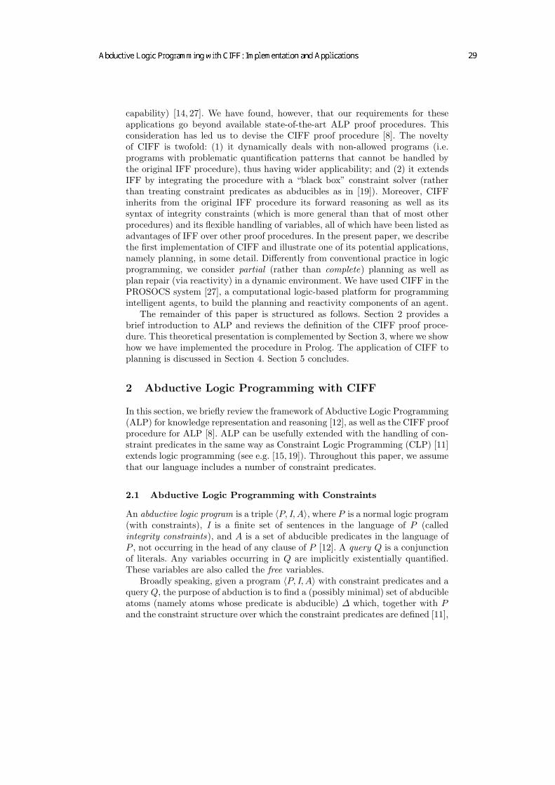
capability) [14, 27]. We have found, however, that our requirements for theseapplications go beyond available state-of-the-art ALP proof procedures. Thisconsideration has led us to devise the CIFF proof procedure [8]. The noveltyof CIFF is twofold: (1) it dynamically deals with non-allowed programs (i.e.programs with problematic quantification patterns that cannot be handled bythe original IFF procedure), thus having wider applicability; and (2) it extendsIFF by integrating the procedure with a “black box” constraint solver (ratherthan treating constraint predicates as abducibles as in [19]). Moreover, CIFFinherits from the original IFF procedure its forward reasoning as well as itssyntax of integrity constraints (which is more general than that of most otherprocedures) and its flexible handling of variables, all of which have been listed asadvantages of IFF over other proof procedures. In the present paper, we describethe first implementation of CIFF and illustrate one of its potential applications,namely planning, in some detail. Differently from conventional practice in logicprogramming, we consider partial (rather than complete) planning as well asplan repair (via reactivity) in a dynamic environment. We have used CIFF in thePROSOCS system [27], a computational logic-based platform for programmingintelligent agents, to build the planning and reactivity components of an agent.

The remainder of this paper is structured as follows. Section 2 provides abrief introduction to ALP and reviews the definition of the CIFF proof proce-dure. This theoretical presentation is complemented by Section 3, where we showhow we have implemented the procedure in Prolog. The application of CIFF toplanning is discussed in Section 4. Section 5 concludes.

2 Abductive Logic Programming with CIFF

In this section, we briefly review the framework of Abductive Logic Programming(ALP) for knowledge representation and reasoning [12], as well as the CIFF proofprocedure for ALP [8]. ALP can be usefully extended with the handling of con-straint predicates in the same way as Constraint Logic Programming (CLP) [11]extends logic programming (see e.g. [15, 19]). Throughout this paper, we assumethat our language includes a number of constraint predicates.

2.1 Abductive Logic Programming with Constraints

An abductive logic program is a triple 〈P, I, A〉, where P is a normal logic program(with constraints), I is a finite set of sentences in the language of P (calledintegrity constraints), and A is a set of abducible predicates in the language ofP , not occurring in the head of any clause of P [12]. A query Q is a conjunctionof literals. Any variables occurring in Q are implicitly existentially quantified.These variables are also called the free variables.

Broadly speaking, given a program 〈P, I, A〉 with constraint predicates and aquery Q, the purpose of abduction is to find a (possibly minimal) set of abducibleatoms (namely atoms whose predicate is abducible) ∆ which, together with Pand the constraint structure over which the constraint predicates are defined [11],

“entail” (an appropriate ground instantiation of) Q, with respect to a suitablenotion of “entailment”, in such a way that the extension of P with this set“satisfies” I (see [12] for possible notions of integrity constraint satisfaction).The appropriate notion of “entailment” depends on the semantics associatedwith the logic program P (again, there are several possible choices for such asemantics [12]). In the remainder of this paper we will adopt the completionsemantics [4, 20] for logic programming, and extend it a la CLP to take theconstraint structure into account. We represent entailment under such semanticsas |=<. An abductive answer to a query Q for a program 〈P, I, A〉, containingconstraint predicates defined over a structure <, is a pair 〈∆, σ〉, where ∆ is aset of ground abducible atoms and σ is a substitution for the free variables in Qsuch that P ∪∆σ |=< I ∧Qσ.

2.2 The CIFF Proof Procedure

We now give a brief description of the CIFF procedure [8]. Like Fung and Kowal-ski [10], we require the theory given as input to be represented in “iff-form” [4,10], which we can obtain by selectively completing P with respect to all predi-cates except special predicates (true, false, constraint and abducible predicates).That is, an alternative representation of an abductive logic program would be apair 〈Th, I 〉, where Th is a set of (homogenised) iff-definitions:

p(X1, . . . , Xk)⇔ D1 ∨ · · · ∨Dn

Here, p must not be a special predicate and there can be at most one iff-definitionfor every predicate symbol. Each of the disjuncts Di is a conjunction of literals.The variables X1, . . . , Xk are implicitly universally quantified with the scope be-ing the entire definition. Any other variable is implicitly existentially quantified,with the scope being the disjunct in which it occurs.

In this paper, the set of integrity constraints I are implications of the form:

L1 ∧ · · · ∧ Lm ⇒ A1 ∨ · · · ∨An

Each of the Li must be a literal; each of the Ai must be an atom. Any variablesare implicitly universally quantified with the scope being the entire implication.

In CIFF, the search for abductive answers of queries over a proof tree isinitialised with the root of the tree consisting of the integrity constraints in theprogram and the literals of the query. The procedure then repeatedly manipu-lates the current node by applying equivalence-preserving proof rules to it. Thenodes are sets of formulas (the so-called goals) which may be atoms, implica-tions, or disjunctions of literals. The implications are either integrity constraints,their residues, or obtained by rewriting negative literals (e.g. not p is rewritten asp⇒ false.) The proof rules modify nodes by rewriting goals in them, adding newgoals to them, or deleting superfluous goals from them. The set of iff-definitionsis kept in the background and is only used to unfold defined predicates.

Fung and Kowalski [10] require inputs to their proof procedure to meeta number of allowedness conditions (essentially avoiding certain problematic

patterns of quantification) to be able to guarantee its correct operation. Theseconditions are overly restrictive; IFF could produce correct answers also forsome non-allowed inputs. Unfortunately, it is difficult to formulate appropriateallowedness conditions that guarantee a correct execution of the proof proce-dure without imposing too many unnecessary restrictions. Our proposal, putforward in [8], is to tackle the issue of allowedness dynamically, i.e. at runtime,rather than adopting a static and overly strict set of conditions. To this end,CIFF includes a dynamic allowedness rule amongst its proof rules, which getstriggered once the procedure encounters, in the current node, formulas it cannotmanipulate correctly due to a problematic quantification pattern. When thishappens, the node is labelled as undefined and will not be selected again. Inaddition to the dynamic allowedness rule, the main proof rules of CIFF are:

– Unfolding: Replace any atomic goal p(~t), for which there is a definitionp( ~X) ⇔ D1 ∨ · · · ∨ Dn in Th, by (D1 ∨ · · · ∨ Dn)[ ~X/~t]. There is a simi-lar rule for defined predicates inside implications.

– Splitting: Rewrite any node with a disjunctive goal as a disjunction of nodes.– Propagation: Given goals of the form p(~t) ∧ A ⇒ B and p(~s), add the goal

(~t = ~s) ∧A⇒ B.– Case analysis for constraints: Replace any goal of the form Con ∧ A ⇒ B,

where Con is a constraint not containing any universally quantified variables,by [Con∧(A⇒ B)]∨Con. There is a similar case analysis rule for equalities.

– Constraint solving: Replace any node containing an unsatisfiable set of con-straints (as atoms) by false.

In addition, there are logical simplification rules, rules for rewriting equalitiesand making substitutions, and rules that reflect the interplay between constraintpredicates and the usual equality predicate. For full details we refer to [8].

In a proof tree for a query, a node containing false is called a failure node.If all leaf nodes are failure nodes, then the search is said to fail. A node towhich no more proof rules can be applied is called a final node. A final node thatis not a failure node and which has not been labelled as undefined is called asuccess node. If a success node exists, then the search is said to succeed. CIFFhas been proved sound in [8]: it is possible to extract an abductive answer fromany success node (soundness of success); and if the search fails then there existsno such answer (soundness of failure).

3 Implementation of the Proof Procedure

We have implemented the CIFF procedure in Sicstus Prolog [28].3 Most of thecode could very easily be ported to any other Prolog system conforming tostandard Edinburgh syntax. A minor exception is the module concerned withconstraint solving as it relies on Sicstus’ built-in constraint logic programmingsolver over finite domains (CLPFD) [3]. However, the modularity of our imple-mentation would make it relatively easy to integrate a different constraint solver3 The system is available at http://www.doc.ic.ac.uk/∼ue/ciff/

lamp(X) iff [[X=a]].

battery(X,Y) iff [[X=b, Y=c]].

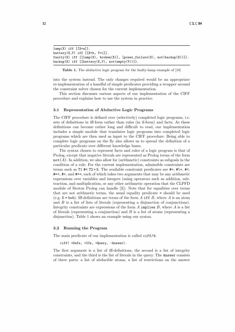
faulty(X) iff [[lamp(X), broken(X)], [power_failure(X), not(backup(X))]].

backup(X) iff [[battery(X,Y), not(empty(Y))]].

Table 1. The abductive logic program for the faulty-lamp example of [10]

into the system instead. The only changes required would be an appropriatere-implementation of a handful of simple predicates providing a wrapper aroundthe constraint solver chosen for the current implementation.

This section discusses various aspects of our implementation of the CIFFprocedure and explains how to use the system in practice.

3.1 Representation of Abductive Logic Programs

The CIFF procedure is defined over (selectively) completed logic programs, i.e.sets of definitions in iff-form rather than rules (in if-form) and facts. As thesedefinitions can become rather long and difficult to read, our implementationincludes a simple module that translates logic programs into completed logicprograms which are then used as input to the CIFF procedure. Being able tocomplete logic programs on the fly also allows us to spread the definition of aparticular predicate over different knowledge bases.

The syntax chosen to represent facts and rules of a logic program is that ofProlog, except that negative literals are represented as Prolog terms of the formnot(A). In addition, we also allow for (arithmetic) constraints as subgoals in thecondition of a rule. For the current implementation, admissible constraints areterms such as T1 #< T2 + 5. The available constraint predicates are #=, #\=, #<,#=<, #>, and #>=, each of which takes two arguments that may be any arithmeticexpressions over variables and integers (using operators such as addition, sub-traction, and multiplication, or any other arithmetic operation that the CLPFDmodule of Sicstus Prolog can handle [3]). Note that for equalities over termsthat are not arithmetic terms, the usual equality predicate = should be used(e.g. X = bob). Iff-definitions are terms of the form A iff B, where A is an atomand B is a list of lists of literals (representing a disjunction of conjunctions).Integrity constraints are expressions of the form A implies B, where A is a listof literals (representing a conjunction) and B is a list of atoms (representing adisjunction). Table 1 shows an example using our syntax.

3.2 Running the Program

The main predicate of our implementation is called ciff/4:

ciff( +Defs, +ICs, +Query, -Answer).

The first argument is a list of iff-definitions, the second is a list of integrityconstraints, and the third is the list of literals in the query. The Answer consistsof three parts: a list of abducible atoms, a list of restrictions on the answer

substitution, and a list of constraints (the latter two can be used to constructan answer substitution according to the semantics of ALP).

Alternatively, the first two arguments of ciff/4 may be replaced with thename of a file containing an abductive logic program. An example for such a fileis given in Table 1. This is the faulty-lamp example discussed, amongst others,by Fung and Kowalski [10]. The syntax is almost self-explanatory (recall that alist of lists represents a disjunction of conjunctions). This program happens toconsist only of iff-definitions (there are no integrity constraints). Assuming thatthe program is stored in a file called lamp.alp, we may run the following query:

?- ciff( ’lamp.alp’, [faulty(X)], Answer).

Answer = [broken(a)]:[X/a]:[] ? ;

Answer = [empty(c),power_failure(b)]:[X/b]:[] ? ;

Answer = [power_failure(X)]:[not(X/b)]:[] ? ; No

Here the user has enforced backtracking, so all three answer are being reportedby the system. Note that the third (empty) list in each of the answers would beused to store the associated constraints (of which there are none in this example).For details on how to interpret the above answers, we refer to [10].

3.3 Implementation of the Proof Rules

We are now going to turn our attention to the actual implementation of the proofprocedure and explain some of the design decisions taken during its development.Our implementation of CIFF has been inspired by work in the Automated Rea-soning community on so-called lean theorem provers [1]. Our proof proceduremanipulates a list of formulas rather than submitting these formulas themselvesto the Prolog interpreter. One advantage of this approach is, for instance, thatwe can report variable substitutions at the meta-level rather than having Prologmaking the actual instantiations (which would be problematic as CIFF computesonly restrictions on the answer substitution, rather than an actual substitution).

The proof rules are repeatedly applied to the current node. Whenever adisjunction is encountered, it is split into a set of successor nodes (one for eachdisjunct). The procedure then picks one of these successor nodes to continuethe proof search and backtracking over this choicepoint results in all possiblesuccessor nodes being explored. In theory, the choice of which successor node toexplore next is taken nondeterministically; in practice we simply move throughnodes from left to right. The procedure terminates when no more proof rulesapply (to the current node) and finishes by extracting an answer from this node.Enforced backtracking will result in the next branch (if any) of the proof treebeing explored, i.e. in any remaining abductive answers being enumerated. TheProlog predicate implementing the proof rules has the following form:

sat( +Node, +EV, +CL, +LM, +Defs, +FreeVars, -Answer).

Node is a list of goals, representing a conjunction. EV is used to keep track ofexistentially quantified variables in the node. This set is relevant to assess theapplicability of some of the proof rules. CL (for constraint list) is used to store the

constraints that have been accumulated so far. The next argument, LM (for loopmanagement), is a list of expressions of the form A:B recording pairs of formulasthat have already been used with particular proof rules, thereby allowing us toavoid loops that would result if these rules were applied over and over to thesame arguments (this is necessary, for instance, for the propagation rule). Thisinformation can also be exploited to improve efficiency by identifying redundantproof steps. Defs is the list of iff-definitions in the theory. FreeVars is used tostore the list of free variables. Finally, running sat/7 will result in the variableAnswer to be instantiated with a representation of the abductive answer foundby the procedure.

Each proof rule corresponds to a Prolog clause in the implementation ofsat/7. For example, the unfolding rule for atoms is implemented as follows:

sat( Node, EV, CL, LM, Defs, FreeVars, Answer) :-

member( A, Node), is_atom( A), get_def( A, Defs, Ds),

delete( Node, A, Node1), NewNode = [Ds|Node1], !,

sat( NewNode, EV, CL, LM, Defs, FreeVars, Answer).

The auxiliary predicate is atom/1 will succeed whenever the argument rep-resents an atomic goal. Furthermore, get def(A,Defs,Ds), with the first twoarguments being instantiated at the time of calling the predicate, will instanti-ate Ds with the list of lists representing the disjunction that defines the atom Aaccording to the iff-definitions in Defs whenever there is such a definition (i.e.the predicate will fail for abducibles). Once get def(A,Defs,Ds) succeeds wedefinitely know that the unfolding rule is applicable: there exists an atomic con-junct A in the current Node and it is not abducible. The cut in the penultimateline is required, because we do not want to allow any backtracking over the orderin which rules are being applied. After we are certain that this rule should beapplied we manipulate the current Node and generate its successor NewNode. Wefirst delete the atom A and then replace it with the disjunction Ds. The predicatesat/7 then recursively calls itself with the new node.

3.4 Testing

The Prolog clauses in the implementation of sat/7 may be reordered almostarbitrarily (the only requirement is that the clause used to implement answerextraction is listed last). Each order of clauses corresponds to a different proofstrategy, as it implicitly assigns different priorities to the different proof rules.This feature of our implementation allows for an experimental study of whichstrategies yield the fastest derivations. We hope to be able to exploit this featureof the implementation in our future work to study possible optimisation tech-niques. The order in which proof rules are applied in the current implementationfollows some simple heuristics. For instance, logical simplification rules as wellas rules to rewrite equality atoms are always applied first. Splitting, on the otherhand, is one of the last rules to be applied.

The implementation of the CIFF proof procedure has been tested successfullyon a number of examples. Most of these examples are taken from applications

holds(F, T2) ← happens(A, T1), initiates(A, T1, F ), not clipped(T1, F, T2), T1 <T2

holds(F, T ) ← initially(F ), not clipped(0, F, T ), 0 < Tholds(¬F, T2)← happens(A, T1), terminates(A, T1, F ), not declipped(T1, F, T2), T1 <T2

holds(¬F, T ) ← initially(¬F ), not declipped(0, F, T ), 0 < T

clipped(T1, F, T2) ← happens(A, T ), terminates(A, T, F ), T1≤T <T2

declipped(T1, F, T2)← happens(A, T ), initiates(A, T, F ), T1≤T <T2

happens(A, T )← assume happens(A, T )

Table 2. Domain-independent rules in Pplan

holds(F, T ), holds(¬F, T ) ⇒ falseassume happens(A, T ), precondition(A, P ) ⇒ holds(P, T )assume happens(A, T2), not executed(A, T2), time now(T1) ⇒ T1 <T2

Table 3. Domain-independent integrity constraints in Iplan (for complete planning)

of CIFF within the SOCS project, which investigates the application of compu-tational logic-based techniques to multiagent systems (e.g. the implementationof an agent’s planning and a reactivity capabilities). While these are encourag-ing results, it should also be noted that this is only a first prototype and moreresearch into proof strategies for CIFF as well as a fine-tuning of the implemen-tation are required to achieve satisfactory runtimes for larger examples.

4 An Application to Abductive Planning

In this section, as an example application of the CIFF system, we consider howit can be used for planning. For this purpose we propose an abductive versionof the event calculus. The event calculus is a formalism for reasoning aboutevents (or actions) and change formulated by Kowalski and Sergot [18]. Sinceits publication a number of abductive variants of it have been proposed in theplanning and abduction literature [23, 25, 26]. Our formulation is a novel variant,in part inspired by the E-language [16], to allow situated, resource-boundedagents to generate partial plans in a dynamic environment, possibly inhabitedby other agents. Partial planning is useful for two reasons. Firstly, it allows theagents to interleave planning, sensing and acting. Secondly, it prevents agentsfrom spending time and effort constructing complete plans that may becomeunnecessary or unfeasible when they get round to executing them.

4.1 An Abductive Formulation of the Event Calculus

We model a planning problem within the framework of the event calculus(EC) in terms of a (non-allowed) abductive logic program with constraintsKBplan = 〈Pplan, Iplan, Aplan〉. In a nutshell, the EC allows us to write meta-logic programs which “talk” about object-level concepts of fluents, actions, andtime points. The main meta-predicates of the formalism are: holds(F, T ) (fluent

F holds at time T ), clipped(T1, F, T2) (fluent F is clipped —from holding to notholding— between times T1 and T2), declipped(T1, F, T2) (fluent F is declipped—from not holding to holding— between times T1 and T2), initially(F ) (fluentF holds from the initial time, say time 0), happens(A, T ) (action A occurs attime T ), initiates(A, T, F ) (fluent F starts to hold after action A at time T ) andterminates(A, T, F ) (fluent F ceases to hold after action A at time T ). Roughlyspeaking, in a planning setting the last two predicates represent the cause-and-effects links between actions and fluents in the modelled world. We will also usea meta-predicate precondition(A,F ) (the fluent F is one of the preconditions forthe executability of action A). In our KBplan, we allow fluents to be positive(F ) or negative (¬F ). Our formulation of the EC also contains the predicatesobserved/2, executed/2, time now/2, assume holds/2, and assume happens/2,which will be described shortly.

We now define KBplan. To this end we first show the KBplan that wouldbe used for complete planning (but by situated agents, interacting with theirenvironment) and then show how it can be modified to allow for partial plan-ning. Pplan consists of three parts: domain-independent rules, domain-dependentrules, and a narrative part. Iplan consists of domain-independent integrity con-straints and possibly domain-dependent integrity constraints. The basic rulesand integrity constraints for the domain-independent part, adapted from theoriginal EC, are shown in Tables 2 and 3. The only abducible predicate here isassume happens. The reason why we do not use the happens predicate as an ab-ducible and instead define it in terms of assume happens will become clear whenwe describe the (domain-independent) bridging rules given in Table 4. The firstof the integrity constraints given in Table 3 states that a fluent and its negationcannot hold at the same time, while the second one expresses that when assum-ing (planning) that some action will happen, we need to enforce that each of itspreconditions hold. The third constraint ensures that the actions in the resultingplan that have not been executed yet are scheduled for the future.

The domain-dependent rules define the predicates initiates, terminates, andprecondition (as well as any other predicates required by the modelling of theconcrete domain). An example is given in Table 6 (see also Section 4.3). Thefirst two rules state that catching a train or driving to a destination X initiatesbeing at X. The two initially-facts state that initially A has petrol but does nothave any anti-freeze. The last integrity constraint has the flavour of a reactiverule and it states that if you are planning to drive somewhere and you haveobserved shortly before that it is snowing then you must make sure that youhave anti-freeze. The other rules and constraints are self-explanatory.

The narrative part of Pplan defines the predicates initially, observed andexecuted. For instance, initially(at(bob, (1, 1))) expresses that agent bob is initiallyat location (1, 1); executed(go(bob, (1, 1), (2, 2), 3), 5) says that bob went fromlocation (1, 1) to location (2, 2) at time 3, and this has been observed at time 5by the agent who contains it in its Pplan; and observed(at(jane, (2, 2)), 5) statesthat jane is observed to be at location (2, 2) at time 5. The narrative part is notonly domain-dependent, but it also refers to a particular “running scenario”, in

holds(F, T2) ← observed(F, T1), not clipped(T1, F, T2), T1≤T2

holds(¬F, T2) ← observed(¬F, T1), not declipped(T1, F, T2), T1≤T2

clipped(T1, F, T2) ← observed(¬F, T ), T1≤T <T2

declipped(T1, F, T2) ← observed(F, T ), T1≤T <T2

happens(A, T ) ← observed(A, T )happens(A, T ) ← executed(A, T )

Table 4. Domain-independent bridging rules in Pplan

holds(F, T ), assume holds(¬F, T ) ⇒ falseassume holds(F, T ), holds(¬F, T ) ⇒ falseassume happens(A, T ), precondition(A, P ) ⇒ assume holds(P, T )

Table 5. Domain-independent integrity constraints in Iplan (for partial planning)

some concrete circumstances. Typically, executed facts within the narrative partof KBplan of an agent refer to actions executed by the agent, whereas observedfacts refer to properties of the environment, via facts of the form observed(L, T )(the fluent literal L has been observed to hold at time T ) as well as actionsexecuted by other agents, via facts of the form observed(A, T ) (the action A hasbeen observed to have happened at time T ). The parameters of A can containthe identification of the agent who has executed the action. To accommodateobservations, we add the bridging rules shown in Table 4 to Pplan. Note that thenarrative part of Pplan changes over the life time of the agent (whereas the otherparts of the knowledge base remain fixed).

Planning is done by reasoning with Pplan and Iplan to generate appropriateinstances of the abducible predicate assume happens, the successful executionof whose actions would establish the planning goal. Note that we need such apredicate (and happens cannot be used directly), because abducible predicatescannot be defined in the theory.

Now we show how KBplan can be modified to facilitate partial planning.A partial plan contains subgoals as well as actions. Such subgoals are modelledusing an additional abducible predicate assume holds. Table 5 lists the additionalintegrity constraints in KBplan pertaining, specifically, to partial planning. Thepurpose of the first two of the additional integrity constraints is to make surethat no fluent is assumed to hold at a time when the contrary of the fluent holds.The final constraint replaces the second constraint in Table 3.

This formulation allows the agent to plan for its goals by generating actionsand subgoals that correspond to the preconditions of the actions, all of which areconsistent with one another and with the observations that have been made. (Analternative formulation for partial planning can add the integrity constraints ofTable 5 without modifying those in Table 3, but instead adding the following ruleto Pplan: holds(F, T ) ← assume holds(F, T ). This would allow a more “liberal”way of partial planning, but for computational reasons we have chosen the firstapproach in the implementation.)

To summarise, our abductive formulation of the EC for partial planningconsists of KBplan = 〈Pplan, Iplan, Aplan〉, where

– Pplan consists of the rules in tables 2 and 4 and any domain-dependent rules,– Iplan consists of the integrity constraints in Table 5 and the first and last

constraints in Table 3 and any domain-dependent integrity constraints, and– Aplan consists of the predicates assume happens and assume holds.

Intuitively, our proposal adds to more conventional abductive EC theories forplanning the possibility to interact with the environment, by observing thatproperties hold and that other agents have executed actions. These additionspave the way to the situatedness of the agent in the environment, when plan-ning is performed within a “sense-plan-act” cycle. Indeed, observed(L, T ) andobserved(A, T ) facts (where A is an action executed by some other agent) areadded to the narrative part of KBplan as the result of a sensing operation of theagent, whereas executed(A, T ) facts (where A is an action executed by the agent)are added as the result of the execution of a planned action in the environment.Each step in the cycle takes place at some concrete time, used to time-stampthe facts recorded in the narrative part of KBplan.

4.2 Goals and Partial Plans in CIFF

Here we describe in more detail how goals and partial plans of an agent arespecified within the framework of the EC. A goal is a conjunction of the formholds(L, T ) ∧ TC, where TC is a set of constraints on T , referred to as thetemporal constraints of the goal. A (partial) plan for a given goal consists of

– a (possibly empty) set of atoms of the form assume happens(A, T ) ∧ TC,where TC is a set of constraints on T , referred to as the Actions in the plan;

– a (possibly empty) set of atoms of the form assume holds(L, T )∧TC, whereTC is a set of constraints on T , referred to as the SubGoals in the plan.

A partial plan for a set of goals is a set of partial plans, one for each individualgoal. Goals, actions, subgoals and temporal constraints will be typically non-ground, and the variables occurring in them are implicitly existentially quantifiedover the set of (partial) plans and goals.

Given a set of goals, GS, where each goal is of the form holds(L, T ) ∧ TC,a (possibly empty) set of subgoals SubGoals, a (possibly empty) set of actionsActions (representing already existing partial plans that we are trying to ex-pand), and a (possibly empty) set of temporal constraints, to compute a partialplan for GS at a time τ , CIFF uses the program 〈Th, I 〉, where Th is a set ofiff-definitions formed by the selective completion of Pplan, given Aplan, and I isthe set of all integrity constraints in Iplan.

To choose a query for CIFF, we first have to select the goals to be planned forin the next round of planning. Let gs(Goals, Time) be a goal selection functionthat takes as input a set of goals Goals of the form holds(L, T )∧TC and a timeof evaluation Time, and returns as output a subset of Goals. We do not give adefinition for such a selection function here. A number of different definitions

initiates(catch train to(X), T, at(X))initiates(drive to(X), T, at(X))initiates(fill up(X), T, have(X)) ← X = petrolinitiates(fill up(X ), T, have(X)) ← X = anti freeze

initially(¬have(anti freeze))initially(have(petrol))

precondition(drive to(X), have(petrol))

assume happens(catch train to(X), T ), holds(train strike, T ) ⇒ falseassume happens(drive to(X), T1), observed(snowing, T2), T1−5≤T2≤T1 ⇒

assume holds(have(anti freeze, T1))

Table 6. Domain-dependent rules in KBplan for the airport example

are possible, for example gs can select those goals that are deemed “urgent”according to some measure of urgency (e.g. how close their times are to Time).Let GS′ = GS ∪ holds(L, T ) ∧ TC | assume holds(L, T ) ∧ TC ∈ SubGoals.Let gs(GS′, τ) = SelectedGoals. CIFF is then invoked with a query including:

(1) all selected goals: the conjunction of all atoms holds(L, T ) ∧ TC, for all thegoals in SelectedGoals;

(2) all non-selected (sub)goals: the conjunction of all assume holds(L′, T ′)∧TCsuch that holds(L′, T ′) ∧ TC is in GS or assume holds(L′, T ′) ∧ TC is inSubGoals, and holds(L′, T ′) ∧ TC is not in SelectedGoals;

(3) time now(τ);(4) the conjunction of all atoms assume happens(A′, T ′) ∧ TC in Actions.

4.3 Example

To illustrate the application of CIFF to planning consider the following scenario.Agent A has the goal of being at the airport before time 10. It knows of twoways of getting there, by train and by car. It has already learned that there is atrain strike. So it plans to drive there. Then it makes two observations, one thatit is low on petrol, and, the other, that it is snowing. So it plans to get petrol toaccommodate the first observation, and knowing that it is short on anti-freezeit reacts to the information about the snow by adding a goal of topping up itsanti-freeze (thus repairing its plan to fit in with its changed environment). Sothrough the cycle of observations and (partial) planning it finally constructs acomplete plan consisting of the three actions of filling up petrol, topping up anti-freeze, and driving to the airport at appropriate times. The domain-dependentand narrative parts of agent A’s KBplan are shown in Table 6.

Suppose we are now at time 4 and we have the goal of being at the airportbefore time 10. The goal given to CIFF would be the following:

holds(at(airport), T ), T < 10, time now(4)

CIFF will return the following partial plan (with 4 < T ′ < 10):

assume holds(have(petrol), T ′), assume happens(drive to(airport), T ′)

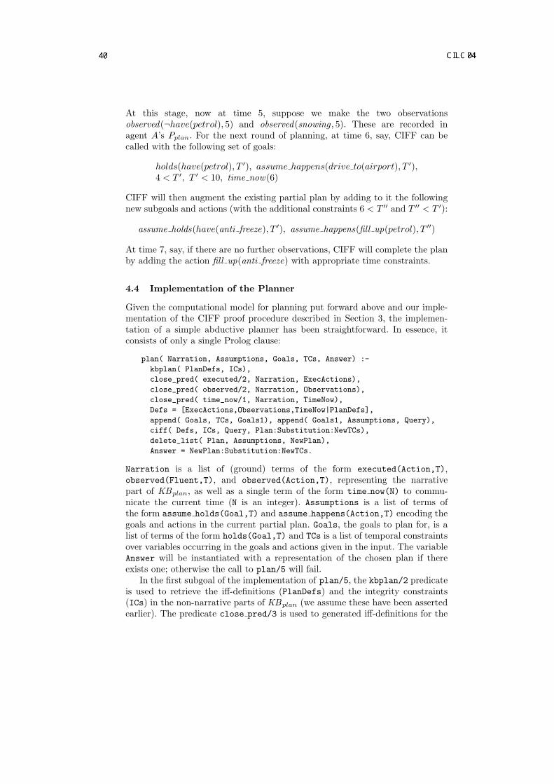
At this stage, now at time 5, suppose we make the two observationsobserved(¬have(petrol), 5) and observed(snowing , 5). These are recorded inagent A’s Pplan. For the next round of planning, at time 6, say, CIFF can becalled with the following set of goals:

holds(have(petrol), T ′), assume happens(drive to(airport), T ′),4 < T ′, T ′ < 10, time now(6)

CIFF will then augment the existing partial plan by adding to it the followingnew subgoals and actions (with the additional constraints 6 < T ′′ and T ′′ < T ′):

assume holds(have(anti freeze), T ′), assume happens(fill up(petrol), T ′′)

At time 7, say, if there are no further observations, CIFF will complete the planby adding the action fill up(anti freeze) with appropriate time constraints.

4.4 Implementation of the Planner

Given the computational model for planning put forward above and our imple-mentation of the CIFF proof procedure described in Section 3, the implemen-tation of a simple abductive planner has been straightforward. In essence, itconsists of only a single Prolog clause:

plan( Narration, Assumptions, Goals, TCs, Answer) :-

kbplan( PlanDefs, ICs),

close_pred( executed/2, Narration, ExecActions),

close_pred( observed/2, Narration, Observations),

close_pred( time_now/1, Narration, TimeNow),

Defs = [ExecActions,Observations,TimeNow|PlanDefs],

append( Goals, TCs, Goals1), append( Goals1, Assumptions, Query),

ciff( Defs, ICs, Query, Plan:Substitution:NewTCs),

delete_list( Plan, Assumptions, NewPlan),

Answer = NewPlan:Substitution:NewTCs.

Narration is a list of (ground) terms of the form executed(Action,T),observed(Fluent,T), and observed(Action,T), representing the narrativepart of KBplan, as well as a single term of the form time now(N) to commu-nicate the current time (N is an integer). Assumptions is a list of terms ofthe form assume holds(Goal,T) and assume happens(Action,T) encoding thegoals and actions in the current partial plan. Goals, the goals to plan for, is alist of terms of the form holds(Goal,T) and TCs is a list of temporal constraintsover variables occurring in the goals and actions given in the input. The variableAnswer will be instantiated with a representation of the chosen plan if thereexists one; otherwise the call to plan/5 will fail.

In the first subgoal of the implementation of plan/5, the kbplan/2 predicateis used to retrieve the iff-definitions (PlanDefs) and the integrity constraints(ICs) in the non-narrative parts of KBplan (we assume these have been assertedearlier). The predicate close pred/3 is used to generated iff-definitions for the

predicates occurring in the Narration and these are appended to the list ofdefinitions to obtain Defs. Then the CIFF proof procedure is called with Defsas the background theory, ICs as the integrity constraints, and the list of all otherrelevant terms as the query. The first component of the answer consists of a listof abducible predicates encoding the plan (using assume holds/2 for subgoalsand assume happens/2 for actions). To simplify the output, the assumptions(goals and actions) already present in the input are then deleted from this list.Furthermore, the answer may also include a list of restrictions on the answersubstitution (Substitution) and an updated list of constraints (NewTCs).

5 Conclusion

We have presented a Prolog implementation of the CIFF procedure that extendsthe general purpose abductive proof procedure IFF by dealing with non-allowedprograms and by handling constraints. The implementation allows the use ofany abductive logic program and presents answers in the form of abducibles withinstantiations and restrictions of variables. We have also discussed an applicationto planning where, by varying the input theory, we can construct complete orpartial plans in the presence or absence of narrative information.

The CIFF system has been used extensively in the PROSOCS framework [27]to implement a planning component as well as for reactivity and temporal rea-soning. Reactivity allows condition-action rule behaviour used in PROSOCS,for example, for plan repair, for strategies for negotiation and communicationwith other agents, and generally for reacting to changes in the environment. Thetemporal reasoning capability is based on an extensive abductive logic programbased on the event calculus that deals with the revision of the agent’s knowl-edge as a result of assimilating new information from its environment, includingother agents [2]. We have been able to use and test the CIFF system on a num-ber of examples for all three applications without any modifications. While sofar, we have concentrated on providing an implementation of CIFF that cor-rectly implements the semantics, that is easy to understand, and that supportsfuture extensions, in our future work we hope to also study possible optimisationtechniques for CIFF.

Acknowledgements. This work was supported by the European Commission FETGlobal Computing Initiative, within the SOCS project (IST-2001-32530). Wethank all SOCS partners for useful feedback and in particular Marco Gavanelliand Michela Milano for suggestions on implementing the constraint solver.

References

1. B. Beckert and J. Posegga. leanTAP: Lean, Tableau-based deduction. J. Auto-mated Reasoning, 15(3):339–358, 1995.

2. A. Bracciali and A. C. Kakas. Frame consistency: Computing with causal expla-nations. In Proc. NMR-2004, 2004. To appear.

3. M. Carlsson, G. Ottosson, and B. Carlson. An open-ended finite domain constraintsolver. In Proc. PLILP-97, 1997.

4. K. L. Clark. Negation as failure. In Logic and Data Bases. Plenum Press, 1978.5. L. Console, D. T. Dupre, and P. Torasso. On the relationship between abduction

and deduction. J. Log. Computat., 1(5):661–690, 1991.6. M. Denecker and D. De Schreye. SLDNFA: An abductive procedure for abductive

logic programs. J. Log. Prog., 34(1):111–167, 1998.7. M. Denecker and B. Van Nuffelen. Experiments for integration CLP and abduction.

In Proc. Workshop on Constraints, 1999.8. U. Endriss, P. Mancarella, F. Sadri, G. Terreni, and F. Toni. The CIFF proof

procedure: Definition and soundness results. Technical Report 2004/2, Departmentof Computing, Imperial College London, 2004.

9. K. Eshghi and R. A. Kowalski. Abduction compared with negation by failure. InG. Levi and M. Martelli, editors, Proc. ICLP-1989. MIT Press, 1989.

10. T. H. Fung and R. A. Kowalski. The IFF proof procedure for abductive logicprogramming. J. Log. Prog., 33(2):151–165, 1997.

11. J. Jaffar and M. J. Maher. Constraint logic programming: A survey. J. Log. Prog.,19-20:503–582, 1994.

12. A. C. Kakas, R. A. Kowalski, and F. Toni. The role of abduction in logic pro-gramming. In Handbook of Logic in Artificial Intelligence and Logic Programming,volume 5, pages 235–324. Oxford University Press, 1998.

13. A. C. Kakas and P. Mancarella. Abductive logic programming. In Proc. WorkshopLogic Programming and Non-Monotonic Logic, 1990.

14. A. C. Kakas, P. Mancarella, F. Sadri, K. Stathis, and F. Toni. The KGP model ofagency. In Proc. ECAI-2004, 2004. To appear.

15. A. C. Kakas, A. Michael, and C. Mourlas. ACLP: Abductive constraint logicprogramming. J. Log. Prog., 44:129–177, 2000.

16. A. C. Kakas and R. Miller. A simple declarative language for describing narrativeswith actions. J. Log. Prog., 31(1–3):157–200, 1997.

17. A. C. Kakas, B. Van Nuffelen, and M. Denecker. A-system: Problem solvingthrough abduction. In Proc. IJCAI-2001. Morgan Kaufmann, 2001.

18. R. A. Kowalski and M. Sergot. A logic-based calculus of events. New GenerationComputing, 4(1):67–95, 1986.

19. R. A. Kowalski, F. Toni, and G. Wetzel. Executing suspended logic programs.Fundamenta Informaticae, 34:203–224, 1998.

20. K. Kunen. Negation in logic programming. J. Log. Prog., 4:289–308, 1987.21. F. Lin and J.-H. You. Abduction in logic programming: A new definition and an

abductive procedure based on rewriting. Artif. Intell., 140(1/2):175–205, 2002.22. P. Mancarella and G. Terreni. An abductive proof procedure handling active rules.

In Proc. AI*IA-2003. Springer-Verlag, 2003.23. L. Missiaen, M. Bruynooghe, and M. Denecker. CHICA, an abductive planning

system based on event calculus. J. Log. Computat., 5(5):579–602, 1995.24. F. Sadri and F. Toni. Abduction with negation as failure for active and reactive

rules. In Proc. AI*IA-1999. Springer-Verlag, 2000.25. M. P. Shanahan. Prediction is deduction but explanation is abduction. In Proc.

IJCAI-1989. Morgan Kaufmann, 1989.26. M. P. Shanahan. Solving the Frame Problem. MIT Press, 1997.27. K. Stathis, A. C. Kakas, W. Lu, N. Demetriou, U. Endriss, and A. Bracciali.

PROSOCS: A platform for programming software agents in computational logic.In Proc. AT2AI-2004, 2004.

28. Swedish Institute of Computer Science. Sicstus Prolog User Manual, 2003.

A multi context-based Approximate Reasoning

Luciano Blandi and Maria I. Sessa

Dipartimento Matematica e InformaticaUniversita’ di Salerno

via Ponte Don Melillo - 84084 Fisciano (SA), Italylblandi, misessa@unisa.it

Abstract. The paper concerns with the theory of similarity relations in the framework ofLogic Programming. Similarity relation [34] is a formal notion that allows us to managealternative instances of entities that can be considered ‘equal’ with a given degree. In [8,15, 30, 29, 18] this notion has been encapsulated in an inference engine, based on the LogicProgramming paradigm, modifying the inference model to provide a more flexible unifica-tion (approximately equal) than the dichotomic match (equal or not). In many situations,more than one similarity relation can be defined in a universe by taking into account differ-ent contexts. In this paper we studied some aggregations of such fuzzy relations and theirapplication to our extented Logic Programming framework.

1 Introduction and previous works

The main interest in Logic Programming field traditionally concerns problems related to the anal-ysis and the efficiency of exact inferences allowed by logic programs [1, 14]. However, very oftenthe need of methods to enhance this capability, in order to deal with approximate information orflexible inference schemes, arises in many applications. In general, approximate reasoning capa-bilities are introduced in the Logic Programming framework by considering the inference systembased on fuzzy logic rather than on conventional two-valued logic.

In [8] a methodology that allows to manage uncertain and imprecise information in the frameof the declarative paradigm of Logic Programming has been proposed. With this aim, a Similarityrelation R between function and predicate symbols in the language of a logic program is considered.Approximate inferences are then possible since Similarity relation allows us to manage alternativeinstances of entities that can be considered ”equal” with a given degree.

With respect to the previous literature [4, 31, 12, 13], this approach is very different since theapproximation is represented and managed at a syntactic-level, instead of at a rule-level. Roughlyspeaking, the basic idea is that the fuzziness feature is provided by an abstraction process whichexploits a formal representation of similarity relations between elements in the alphabet of thelanguage (constants, functions, predicates). On the contrary, in the underground logic theory, theinference rule as well as the usual crisp representation of the considered universe are not modified.It allows us to avoid both the introduction of weights on the clauses, and the use of fuzzy sets aselements of the language.

In [29] the operational counterpart of this extension is faced by introducing a modified SLDResolution procedure. Such a procedure allows us to compute numeric values belonging to theinterval [0,1] providing an approximation measure of the obtained solutions. These numeric valuesare computed through a generalized unification mechanism. In [18] a Prolog interpreter written inJava which implements this Similarity-based extension has been presented.

In these works, the approximation was based on a single similarity relation. However, by takinginto account different contexts (i.e. points of view), it is possible to define different similarityrelations in a given universe. Let us consider the following Example

Multi context-based Approximate Reasoning 2

Example 1.Let U be a set of animals denoted with

U = M, B, G, E, P, H, S, T, C, W, D

where these letters stand for

M = man, B = bear, G = gorilla, E = eagle, P = pigeon, H = hawk,

S = shark, T = tiger, C = cat, W = wolf , D = dog.

We can define a similarity R1 between elements in U based on feature ‘morphology’ by setting forany x, y ∈ U

R1(x, y) = R1(y, x)

R1(x, y) = 1 if x = y

R1(G,M) = R1(D,W ) = R1(E,H) = .8

R1(W,T ) = R1(D,T ) = .6

R1(C, T ) = R1(C,W ) = R1(C,D) = .4

R1(B, T ) = R1(B,C) = R1(B,W ) = R1(B,D) = R1(E,P ) = R1(P,H) = .2

R1(x, y) = 0 otherwise.

Also, we can define a similarity R2 between elements in U based on feature ‘aggressiveness’ bysetting for any x, y ∈ U

R2(x, y) = R2(y, x)

R2(x, y) = 1 if x = y

R2(G,W ) = R2(T, S) = R2(E,H) = .8

R2(M,D) = R2(B,S) = R2(B, T ) = R2(C,D) = .6

R2(M,E) = R2(M,H) = R2(M,C) = R2(B,G) = R2(B,W ) = R2(G,S) == R2(G,T ) = R2(E,C) = R2(E,D) = R2(H,C) = R2(H,D) = R2(S,W ) = R2(T,W ) = .4

R2(M,B) = R2(M,G) = R2(M,S) = R2(M,T ) = R2(W,M) = R2(B,E) == R2(B,H) = R2(B,C) = R2(B,D) = R2(G,E) = R2(G,H) = R2(G,C) = R2(G,D) == R2(E,S) = R2(E, T ) = R2(E,W ) = R2(H,S) = R2(H,T ) = R2(H,W ) = R2(S,C) =

= R2(S,D) = R2(T,C) = R2(T,D) = R2(C,W ) = R2(W,D) = .2

R2(x, y) = 0 otherwise.

In many cases, we may need to aggregate different relations. Aggregation of binary (fuzzy)relations is an important and challenging mathematical problem in applied areas as social choice,group choice, multiple-criteria decision-making, synthesis of implication functions, etc. Formally,this problem can be formulated in terms of group choice theory as follows: suppose U is a finite set ofalternatives and R =< R1, ..., Rn > is an ordered n-tuple of binary (fuzzy) relations on U. Elementsof R are regarded as individual preferences and R is called a profile of individual preferences onthe set U of alternatives. For a given U, an aggregation rule assigns a group preference R to eachprofile R of individual preferences on U (very often it is assumed that n > 2). We denote this ruleby the same letter R. Depending on the application area, various restrictions are imposed on R. In[5, 11, 2, 26, 27, 21, 28], the fuzzy binary relations R1, ..., Rn and R satisfy T-transitivity propertyin which T is an Archimedian t-norm. In our framework we consider transitivity based on theminimum triangular norm. In particular, in this paper we study properties of Rmin =

⋂i Ri and

Rmax =⋃

i Ri assuming that individual and group preferences are similarity relations on a finiteset of alternative U.

The paper is organized as follows. After preliminaries on similarity relation in Logic Pro-gramming framework, Section 3 will study the aggregation of similarity relations by intersection(Subsection 3.1) and union (Subsection 3.2), and their exploitation in the similarity based LogicProgramming (Subsection 3.3). The last section contains some concluding remarks.

Multi context-based Approximate Reasoning 3

2 Preliminaries

2.1 Similarity relation

An important and very intuitive theoretical basis for fuzzy subsets is given by the concept offuzzy equivalence relations, which, in some sense, measure the degree to which two points of theuniverse are indistinguishable, and which generalize and relax the concept of classical equivalencerelations. A strong motivation for this notion follows from the so-called Poincare Paradox [25]: iffor three (real world) objects A, B and C we know that A is indistinguishable from B and B isindistinguishable from C, we cannot necessarily conclude that A is indistinguishable from C too.Fuzzy equivalence relations have been introduced under the name of similarity relation in [34](with respect to the minimum TM , the generalization to t-norms was considered in [32]). In thissection, we will recall some well-known definitions and properties related to similarity relation andto its application in the Logic Programming framework.

In Cantorian set theory, a relation on a universe U can be identified with a subset of U2. Byanalogy, a fuzzy relation on U is then a fuzzy subset of U2. For early traces of properties of fuzzyrelations see [34] and [22–24], more recent treatments include [6, 3].

At first, let us recall that a T-norm is a binary operation ∧ : [0, 1] × [0, 1] → [0, 1] associative,commutative, non-decreasing in both the variables, and such that x ∧ 1 = 1 ∧ x = x for any x in[0,1]. In the sequel, we assume that x ∧ y is the minimum between the two elements x, y ∈ [0, 1].

Definition 1. Given a T-norm, a fuzzy relation R on a set U is T-transitive if and only ifT (R(x, y), R(y, z)) ≤ R(x, z) for any x, y, z ∈ U.

Among all T-transitive fuzzy relations, similarity relations and fuzzy T-preorders are the mostimportant ones.

Definition 2. A similarity on a domain U is a fuzzy relation R : U × U → [0, 1] in U such thatthe following properties hold

i) R(x, x) = 1 for any x ∈ U (reflexivity)

ii) R(x, y) = R(y, x) for any x, y ∈ U (symmetry)

iii) R(x, z) ≥ R(x, y) ∧ R(y, z) for any x, y, z ∈ U (transitivity)

we say that R is strict if the following implication is also verified

iv) R(x, z) = 1 =⇒ x = z.

The value R(x, z) can be interpreted as the degree of equality or the degree of indistinguishabil-ity of x and y or, equivalently, as the truth value of the statement ’x is equal to y’. The ∧-transitivityis a many-valued model of the proposition ’IF x is equal to y AND y is equal to z THEN x is equalto z’.

Similarities also are called indistinguishability operators, fuzzy equalities, fuzzy equivalences,likeness, probabilistic relations, proximity relations, M-valued equality, depending on the authorsand on the t-norm used to model their transitivity.

There is a lot of work around this concept and it has been proved to be a useful tool both inthe theoretical aspects of fuzzy logic and in their applications such as fuzzy control or approximatereasoning.

Multi context-based Approximate Reasoning 4

2.2 Similarity relation and closure operators

We synthetically give some well known notions concerning closure operators and equivalence rela-tions.

Definition 3. Let (P,¹) be a poset. An operator H : P → P is called a closure (resp. reductive)operator if for any x, y in P the following properties hold:

i) x ¹ H(x) (resp. H(x) ¹ x)

ii) H(H(x)) = H(x)

iii) x ¹ y =⇒ H(x) ¹ H(y).

Proposition 1. Let ≡ be an equivalence relation on a set S and P(S) the powerset of S. Then,the operator H≡ : P(S) → P(S) such that for any X ⊆ P(S)

H≡(X) = x′ ∈ S | ∃x ∈ X : x′ ≡ x)

is a closure operator.

The following notion of λ−cut is crucial in fuzzy set theory:

Definition 4. Let U be a domain and R : U × U → [0, 1] a fuzzy relation in U . Then, for anyλ ∈ [0, 1], the relation ≅R,λ in U defined as

x ≅R,λ y ⇐⇒ R(x, y) º λ

is named cut of level λ (in short λ-cut) of R.

Similarity relations are strictly related with equivalence relations and, then, to closure opera-tors. Indeed, the notion of λ− cut allows us to define a similarity by means of a suitable family ofequivalence relations according to the following result that can be easily proven.

Proposition 2. Let U be a domain and R : U × U → [0, 1] a Similarity in U . Then, for any λ ∈[0, 1], the relation ≅R,λ in U is an equivalence relation. Also, the operator H≅R,λ

: P(U) → P(U)such that for any X ∈ P(U)

H≅R,λ(X) = z ∈ U | ∃x ∈ X : x ≅R,λ y = z ∈ U | ∃x ∈ X : R(z, x) ≥ λ ,

is a closure operator.

Proposition 3. Let R be a similarity in a domain U and, for any λ ∈ [0, 1] let ≅R,λ be the λ−cutof R. Then, ≅R,λλ∈[0,1] is a family of equivalence relations such that,

i) for any µ and λ in [0, 1], λ ¹ µ ⇒ ≅R,λ ⊇ ≅R,µ

ii) for any µ in [0, 1],⋂

λ¹µ

≅R,λ = ≅R,µ .

Conversely, let ≅λλ∈[0,1] be a family of equivalence relations satisfying conditions i) and ii).Then the relation R defined by setting

R(x, y) = Supλ ∈ [0, 1] | x ≅λ y

is a similarity whose family of λ−cuts is equal to the family ≅λλ∈[0,1].

Any λ−cut can be considered as a generalization of the equality. This notion plays an importantrule in our approach. Indeed, the relation ≅R,λ formalizes the idea that two constant symbols canbe considered equal with a fixed approximation level λ ∈ [0, 1]. Such a level provides a measureof the allowed approximation in order to avoid failure of matching between constant symbols in aSLD-derivation process.

Multi context-based Approximate Reasoning 5

2.3 Logic Programming with Similarity

We briefly recall that a logic program P is a set of universally quantified Horn clauses on a firstorder language L, denoted with H ← B1, . . . , Bk, and a goal is a negative clause, denoted withA1, . . . , An. We denote with BL the set of ground atomic formulae in L, i.e. the Herbrand base ofL, and with TP the immediate consequence operator TP : P(BL) 7→ P(BL) defined by:

TP (X) = a|a ← a1, . . . , an ∈ Γ (P ) and ai ∈ X, 1 ≤ i ≤ n

where Γ (P ) denotes the set of all ground instances of clauses in P . The application of Tarski’sfixpoint theorem yields a characterization of the semantics of P , which is the least Herbrand modelMP of P given by:

MP = lfp(TP ) =⋃

n≥0 TnP (∅)

where lfp stands for least fixpoint [1].In the classical Logic Programming, function and predicate symbols of the language L are crisp

elements, i.e., distinct elements represent distinct information and no matching is possible. In [8]the exact matching between different entities is relaxed by introducing a Similarity relation R inthe set of constant, function and predicate symbols in the language of a logic program P. In orderto deal with the approximation introduced by a similarity relation R, the program P is extendedby adding new clauses which are ”similar” at least with a fixed degree λ in (0,1] to the given ones.This program transformation is obtained by considering the closure operator Hλ associated to R.The new logic program

Hλ(Γ (P )) = C ′ ∈ L|∃C ∈ Γ (P ) such that R(C,C ′) ≥ λ,

named extended-program of level λ, allows us to enhance the inference process.An alternative way to manage the information carried on by the Similarity introduced between

function and predicate symbols in P , is given by considering as an unique element different symbolswhich have Similarity degree greater or equal to λ. In other words, we consider the quotient set of≅R,λ as a new alphabet Lλ, where F/ ≅R,λ and R/ ≅R,λ are the sets of function and predicatesymbols, respectively. More formally, let us denote with [s] ∈ Lλ the equivalence class of a symbols ∈ F ∪ R with respect to ≅R,λWe call translation up to ≅R,λ the function:

τλ : F ∪ R 7→ F/ ≅R,λ ∪R/ ≅R,λ

defined by setting:

τλ(x) = x for any variable x ∈ V , and τλ(f) = [f ]

for any function/predicate symbol f ∈ F ∪ R. Recursively, we can easily define the extension ofτλ to the sets of formulae in L. Let us consider a logic program P on the language L.

The set

Pλ = τλ(Γ (P )) = C ′ ∈ Lλ|C′ = τλ(C), C clause in Γ (P )

is a logic program that we name abstract-program of level λ.By considering the abstract program Pλ, it is possible to express information provided by the

similarity relation in a syntectic way exploiting the quotient language Lλ. Then, Pλ could be usedto manage similarity-based reasoning as well as Hλ(Γ (P )). In [30] the equivalence of these twoapproaches has been shown for first order languages by using an abstract interpretation technique.

It is worth to stress that the introduced similarity generally changes the semantic of the originalprogram. Indeed, it allows us to add new clauses to P providing the extended program Hλ(P ).This is the more straight way to implement the approximated inference process based on similarity.

Multi context-based Approximate Reasoning 6

On the other hand, by considering the abstract program Pλ, it is possible to express informationprovided by the similarity relation in a syntectic way exploiting the quotient language Lλ.

Both these programs allow to perform approximate inferences by assuming a “tolerance” levelλ ∈ (0, 1] in the relaxed matching between different function/predicate symbols.

In [8], the formal notion of fuzzy least Herbrand model MP,R : BL 7→ [0, 1] of the program Pwith respect to the Similarity R is defined by setting for any A ∈ BL:

MP,R(A) = Supλ ∈ [0, 1] |A ∈ MHλ(Γ (P ))

= Supλ ∈ [0, 1] |Hλ(Γ (P )) ² A

Roughly speaking, for any A ∈ BL the value MP,R(A) provides the best deduction degree of A, i.e,the best level of approximation λ that allows us to prove A by considering an extended programHλ(Γ (P )). It can be proved that:

MP,R(A) = Supλ ∈ [0, 1] |tλ(A) ∈ MPλ

= Supλ ∈ [0, 1] |Pλ ² τλ(A)

Thus, in order to compute the fuzzy least Herbrand model of a program P extended with aSimilarity R, we can equivalently perform our computations in the extended or in the abstractdomain.

3 On aggregations in multi context-based Logic Programming

framework

In many situations, there can be more than one similarity relation defined in a universe. For exam-ple that we have a set of elements defined by some features. We can generate a similarity relationfrom each feature. In these cases, we must manage and use such information in an appropriatedway, for instance we may need to aggregate the obtained relations. In this Section we give a firstformal environment in order to make that.

3.1 Aggregation of similarity relations by intersection

The most common way to put together a family of T-transitive fuzzy relations is by calculatingtheir minimum (or infimum), which also is a T-transitive relation. Indeed the following well-knownproposition [33] states that x, y are related with respect to R if and only if they are related withrespect to all the relations of the family (because the infimum is used to model the universalquantifier ∀ in fuzzy logic [9]).

Proposition 4. Let (Ri)i∈I be a family of T-transitive fuzzy relations on a set U. The relationdefined for all x, y ∈ U by

R(x, y) = mini∈IRi(x, y)

is a T-transitive fuzzy relation on U.

In particular,

Corollary 1. Let R1, . . . , Rn be n similarity relations on a set U. The relation Rmin =⋂

i Ri

defined for all x, y ∈ U by

Rmin(x, y) = minR1(x, y), . . . , Rn(x, y)

is a similarity relation on U.

Multi context-based Approximate Reasoning 7

Example 2. We consider the similarity relations R1 and R2 defined in Example 1. Then,Rmin(x, y) = Rmin(y, x)

Rmin(x, y) = 1 if x = y

Rmin(E,H) = .8

Rmin(W,T ) = Rmin(C,D) = .4

Rmin(G,M) = Rmin(D,W ) = Rmin(D,T ) = Rmin(C, T ) = Rmin(C,W ) = Rmin(B, T ) == Rmin(B,C) = Rmin(B,W ) = Rmin(B,D) = .2

Rmin(x, y) = 0 otherwise.

3.2 Aggregation of similarity relations by union

The binary fuzzy relation Rmin =⋂

i Ri is an extreme case of aggregation rule because it is veryrestrictive. Indeed, Rmin(a, b) ≤ Ri(a, b) for any i. Many times this way to aggregate fuzzy relationsby intersection leads to undesirable results in applications. The reason is that the minimum has adrastic effect. For instance, if two objects of our universe are very similar or indistinguishable forall but one similarity relation, and for this particular one the similarity value is very low, then theresult applying the minimum will give this last measure and will lose the information of all theother ones. This can be reasonable and useful if we need a perfect matching with respect to allour relations, but this is not the case in many situations. When we need to take all the relationsinto account in a less drastic way, we need to use other ways to aggregate them. A possibility ofsoftening the previous proposition is by replacing the intersection by the union.

We define Rmax =⋃

i Ri by setting Rmax(x, y) = maxR1(x, y), . . . , Rn(x, y).

Note that Rmax not is a similarity relation.

Example 3. We consider the similarity relations R1 and R2 defined in Example 1. Then,Rmax(x, y) = Rmax(y, x)

Rmax(x, y) = 1 if x = y

Rmax(M,G) = Rmax(G,W ) = Rmax(T, S) = Rmax(W,D) = Rmax(E,H) = .8

Rmax(M,D) = Rmax(B,S) = Rmax(B, T ) = Rmax(C,D) = Rmax(T,D) = .6

Rmax(C,W ) = Rmax(T,C) = Rmax(M,E) = Rmax(M,H) = Rmax(M,C) = Rmax(B,G) == Rmax(B,W ) = Rmax(G,S) = Rmax(G,T ) = Rmax(E,C) = Rmax(E,D) =

= Rmax(H,C) = Rmax(H,D) = Rmax(S,W ) = Rmax(T,W ) = .4

Rmax(M,B) = Rmax(M,S) = Rmax(M,T ) = Rmax(W,M) = Rmax(B,E) = Rmax(B,H) == Rmax(P,E) = Rmax(B,C) = Rmax(B,D) = Rmax(G,E) = Rmax(G,H) = Rmax(G,C) == Rmax(P,H) = Rmax(G,D) = Rmax(E,S) = Rmax(E, T ) = Rmax(E,W ) = Rmax(H,S) =

= Rmax(H,T ) = Rmax(H,W ) = Rmax(S,C) = Rmax(S,D) = .2

Rmax(x, y) = 0 otherwise.

Note thatRmax(W, D) = 0.8, Rmax(B, W) = 0.4, Rmax(B, D) = 0.2which violates the min-transitivity property becauseRmax(B, D) ¤ Rmax(W, D) ∧ Rmax(B, W)

Let us recall that the max-T product [34, 33] allows us to construct the transitive closure of agiven reflexive and symmetric fuzzy relation.

Definition 5. Let T be a T-norm and R, S two fuzzy relations in a set U . The max-T (or sup-T )product R S of R and S is the fuzzy relation on U defined by

(R S)(x, y) = supz∈ U

T (R(x, z), S(z, y)) for any x, y ∈ U .

Multi context-based Approximate Reasoning 8

Assuming T continuous, due to the associativity of max-T product, we can define for each n ∈ Nthe power Rn of a fuzzy relation R recursively:

R1 = R,

Rn+1 = R Rn for any n ∈ N .

Definition 6. The T -transitive closure (or T -closure R∗ of a fuzzy relation R on a set U is definedby R∗ = sup

n∈ N

Rn.

Proposition 5. If R is a reflexive and symmetric fuzzy relation on a finite set U of cardinalityn, then R∗ = Rn−1.

Proposition 6. Let R be a reflexive and symmetric fuzzy relation on a set U .

R = R∗ if and only if T (R(x, y), R(y, z)) ≤ R(x, z) for any x, y, z ∈ U .

Therefore, the transitive closure R∗ of a reflexive and symmetric fuzzy relation is a similarityoperator. Moreover, it is straightforward to prove that R∗ is a relation greater or equal than R(R∗ ≥ R). Moreover,it can be shown [33] that if E is a similarity operator greater or equal thanR, then E ≥ R∗. In other words, the transitive closure R∗ of R is the smallest similarity operatorthat contains R and is therefore the best upper approximation of R.

In fact, the following proposition can be proved.

Proposition 7. Given a reflexive and symmetric fuzzy relation R on a set U and R∗ its transitiveclosure. Let A be the set of similarity operators on U greater than or equal to R. Then

R∗(x, y) = infE∈ A

E(x, y).

Example 4. The Min-transitive closure of Rmax defined in Example 3 is

R∗max(x, y) = R∗

max(y, x)

R∗max(x, y) = 1 if x = y

R∗max(M,G) = R∗

max(M,D) = R∗max(M,W ) = R∗

max(G,W ) = R∗max(G,D) = R∗

max(E,H) =

= R∗max(T, S) = R∗

max(W,D) = .8

R∗max(M,C) = R∗

max(M,B) = R∗max(M,S) = R∗

max(M,T ) = R∗max(B,S) = R∗

max(B, T ) =

= R∗max(B,G) = R∗

max(B,W ) = R∗max(B,C) = R∗

max(B,D) = R∗max(G,S) =

= R∗max(G,T ) = R∗

max(G,C) = R∗max(C,D) = R∗

max(T,D) = R∗max(C,W ) =

= R∗max(T,C) = R∗

max(S,W ) = R∗max(T,W ) = R∗

max(S,C) = R∗max(S,D) = .6

R∗max(M,E) = R∗

max(M,H) = R∗max(B,E) = R∗

max(B,H) = R∗max(G,E) = R∗

max(G,H) =

= R∗max(E,C) = R∗

max(E,D) = R∗max(E,S) = R∗

max(E, T ) = R∗max(E,W ) =

= R∗max(H,C) = R∗

max(H,D) = R∗max(H,S) = R∗

max(H,T ) = R∗max(H,W ) = .4

R∗max(M,P ) = R∗

max(B,P ) = R∗max(G,P ) = R∗

max(E,P ) = R∗max(H,P ) = R∗

max(S, P ) =

= R∗max(T, P ) = R∗

max(C,P ) = R∗max(W,P ) = R∗

max(D,P ) = .2.

which is a similarity relation.

3.3 Exploiting Rmin and Rmax in the similarity based Logic Programming

The fuzzy relations Rmin =⋂

i Ri, and Rmax =⋃

i Ri are two extreme cases of aggregation rules.The first one implies that Rmin(a, b) ≤ Ri(a, b) for any i, the second one that Rmax(a, b) ≥ Ri(a, b)for any i. In the sequel we study properties of these relations in the framework of the Similarity-based Logic Programming. Let us start with Rmin.

Multi context-based Approximate Reasoning 9

Proposition 8. Let R1, . . . , Rn be n similarity relations on a set U, let λ ∈ (0, 1] and let P be alogic program. Then,

Hλ,Rmin(Γ (P)) ⊆

n∩

i=1Hλ,Ri

(Γ (P))

Proof. A ∈ Hλ,Rmin(Γ (P)) =⇒ ∃A’ ∈ Γ (P) t.c. Rmin(A, A’) > λ

=⇒minR1(A, A’),...,Rn(A, A’)> λ =⇒Ri(A, A’) > λ ∀i = 1, ..., n=⇒ A ∈ Hλ,Ri

(A’) ∀i = 1, ..., n, A’ ∈ Γ (P) =⇒ A ∈ Hλ,Ri(Γ (P)) ∀i = 1, ..., n

=⇒ A ∈n∩

i=1Hλ,Ri

(Γ (P))

Let us prove that the inverse inclusion does not hold.Let the following logic program be givenP = q(c)←; r(c)←; p(a)←Let us suppose that R1 and R2 are two similarity relations defined in L(P ) such thatR1(r, q) < λ, R1(p, q) > λ, R1(r, p) < λ;R2(r, q) < λ, R2(p, q) < λ, R2(r, p) > λ.Then it follows:Hλ,R1

(Γ (P)) = q(c)←; r(c)←; p(a)←;p(c)←; q(a)←Hλ,R2

(Γ (P)) = q(c)←; r(c)←; p(a)←;p(c)←; r(a)←2∩

i=1Hλ,Ri

(Γ (P)) = q(c)←; r(c)←; p(a)←;p(c)←

Rmin(r, q) < λ, Rmin(p, q) < λ, Rmin(r, p) < λHλ,Rmin

(Γ (P))= q(c)←; r(c)←; p(a)←Results2∩

i=1Hλ,Ri

(Γ (P))* Hλ,Rmin(Γ (P)). ⋄

By the previous result, because the Logic Programming is a monotonic inference system, it followsthat:

MHλ,Rmin(Γ (P )) ⊆ M n

∩i=1

Hλ,Ri(Γ (P ))

Therefore, fixed λ ∈ (0, 1], the extended program w.r.t. Rmin allows to deduce less ground atomicformulae than to the intersection of the extended programs of the similarity relations R1, . . . , Rn.Moreover, we can prove the following result:

Proposition 9. Let R1, . . . , Rn be n similarity relations on a set U, let λ ∈ (0, 1] and let P be alogic program. Then,

M n∩

i=1Hλ,Ri

(Γ (P ))⊆

n∩

i=1MHλ,Ri

(Γ (P ))

Proof. A ∈ M n∩

i=1Hλ,Ri

(Γ (P))= ∪

j>0Tj

n∩

i=1Hλ,Ri

(Γ (P ))

(∅)=⇒ ∃k >1 t.c. A∈Tkn∩

i=1Hλ,Ri

(Γ (P ))

(∅)

=⇒ ∃k>1 t.c. A∈TkHλ,Ri

(Γ (P ))(∅) ∀i = 1, ..., n

=⇒A∈ ∪j>0

TjHλ,Ri

(Γ (P ))(∅) = MHλ,Ri

(Γ (P )) ∀i = 1, ..., n

=⇒A∈n∩

i=1MHλ,Ri

(Γ (P ))

Now let us prove that the inverse inclusion does not hold.Let the following logic program be givenP = q(a)←q(b); q(c)←MP = q(c)Let us suppose that R1 and R2 are two similarity relations defined in L(P ) such thatR1(a,b) < λ, R1(a,c) > λ, R1(b,c) < λ;R2(a,b) < λ, R2(a,c) < λ, R2(b,c) > λ.

Multi context-based Approximate Reasoning 10

Then, it resultsHλ,R1

(Γ (P)) = q(a)←q(b); q(c)←; q(c)←q(b); q(a)←MHλ,R1

(Γ (P )) = q(a), q(c);Hλ,R2

(Γ (P)) = q(a)←q(b); q(c)←; q(a)←q(c); q(b)←MHλ,R2

(Γ (P )) = q(b), q(c), q(a);2∩

i=1MHλ,Ri

(Γ (P )) = q(a), q(c);

2∩

i=1Hλ,Ri

(Γ (P)) = q(a)←q(b); q(c)←

M 2∩

i=1Hλ,Ri

(Γ (P ))= q(c)

Then it results2∩

i=1MHλ,Ri

(Γ (P )) * M 2∩

i=1Hλ,Ri

(Γ (P )). ⋄

Summarizing,

MHλ,Rmin(Γ (P )) ⊆ M n

∩i=1

Hλ,Ri(Γ (P ))

⊆n∩

i=1MHλ,Ri

(Γ (P ))

Thus, let us define the fuzzy least Herbrand model of P w.r.t. the intersection relation Rmin as:

MP,Rmin(A) = supλ ∈ [0, 1] / A ∈ MHλ,Rmin

(Γ (P ))

It can be easily proved that:

Proposition 10. Let R1, . . . , Rn be n strict similarity relations on a set U. Then,A ∈ MP ⇐⇒ MP,Rmin

(A) = 1

Analogous properties hold for R∗max.

Proposition 11. Let R1, . . . , Rn be n similarity relations on a set U, let λ ∈ (0, 1] and let P bea logic program. Then,

n∪

i=1MHλ,Ri

(Γ (P )) ⊆ M n∪

i=1Hλ,Ri

(Γ (P ))

Proof. Let us consider A ∈n∪

i=1MHλ,Ri

(Γ (P )) =⇒ ∃m ∈ 1, . . . , n such as A ∈ MHλ,Rm (Γ (P )) =⇒

=⇒ A ∈ ∪j>0

T jHλ,Rm

(Γ (P ))(∅) =⇒ ∃k>1 such as A ∈ Tk

Hλ,Rm(Γ (P ))

(∅) =⇒ ∃k>1 such as A∈Tkn∪

i=1Hλ,Ri

(Γ (P ))

(∅)

=⇒A∈ ∪j>0

T jn∪

i=1Hλ,Ri

(Γ (P ))

(∅) = M n∪

i=1Hλ,Ri

(Γ (P ))

Let us prove that the inverse inclusion does not hold.Let us consider the following logic programP = p(a)←q(c); r(a)←Let us suppose that R1 and R2 are two similarity relations defined in L(P ) such thatR1(r, q) > λ, R1(p, q) < λ, R1(r, p) < λ, R1(a, c) < λ;R2(r, q) < λ, R2(p, q) < λ, R2(r, p) < λ, R2(a, c) > λ.Then it follows:Hλ,R1

(Γ (P)) = p(a)←q(c); r(a)←; q(a)←; p(a)←r(c)MHλ,R1

(Γ (P )) = q(a), r(a);Hλ,R2

(Γ (P)) = p(a)←q(c); r(a)←; p(c)←q(c); p(a)←q(a); r(c)←MHλ,R2

(Γ (P )) = r(c), r(a);n∪

i=1MHλ,Ri

(Γ (P ))= r(c), r(a), q(a);

Multi context-based Approximate Reasoning 11

2∪

i=1Hλ,Ri

(Γ (P)) = p(a)←q(c); r(a)←; q(a)←; p(a)←r(c); p(c)←q(c)←; p(a)←q(a); r(c)←

Hλ,Ri(Γ (P)) = q(a)←q(b); q(c)←

M 2∪

i=1Hλ,Ri

(Γ (P ))= r(c), r(a), q(a), p(a)

Then, it follows:

M 2∪

i=1Hλ,Ri

(Γ (P ))*

2∪

i=1MHλ,Ri

(Γ (P )). ⋄

Furthermore, it results that

Proposition 12. Let R1, . . . , Rn be n similarity relations on a set U, let λ ∈ (0, 1] and let P bea logic program. Then,

n∪

i=1Hλ,Ri

(Γ (P)) ⊆ Hλ,R∗

max(Γ (P))

Proof. C ∈n∪

i=1Hλ,Ri

(Γ (P)) =⇒ ∃j ∈ 1, . . . , n t.c. C ∈ Hλ,Rj(Γ (P)) =⇒

=⇒ ∃C’ ∈ Γ (P) t.c. Rj(C, C’) > λ =⇒ Rmax(C, C’) > λ =⇒ R∗max(C, C’) > λ =⇒

=⇒ C ∈ Hλ,R∗

max(Γ (P))

Let us prove that the inverse inclusion does not hold.Let us consider two similarity relations R1 ed R2 defined in a first order languages L such thatR1(a, b) = 0.3, R1(a, c) = 0.3, R1(b, c) = 0.5R2(a, b) = 0.6, R2(a, c) = 0.4, R2(b, c) = 0.4thenRmax(a, b) = 0.6, Rmax(a, c) = 0.4, Rmax(b, c) = 0.5andR∗

max(a, b) = 0.6, R∗max(a, c) = 0.5, R∗

max(b, c) = 0.5Let P = a←Then, results thatH0.5,R1

(Γ (P)) = a←H0.5,R2

(Γ (P)) = a←; b←2∪

i=1H0.5,Ri

(Γ (P)) = a←; b←

H0.5,R∗

max(Γ (P)) = a←; b←; c←

Then,

H0.5,R∗

max(Γ (P)) *

2∪

i=1H0.5,Ri

(Γ (P)) ⋄

Then, because the Logic Programming is a monotonic inference systemM n

∪i=1

Hλ,Ri(Γ (P ))

⊆ MHλ,R∗max

(Γ (P ))

Therefore, fixed λ ∈ (0, 1], the extended program w.r.t. R∗max allows to deduce more ground atomic

formulae than to the union of the extended programs of the similarity relations R1, . . . , Rn.

Summarizing,n∪

i=1MHλ,Ri

(Γ (P )) ⊆ M n∪

i=1Hλ,Ri

(Γ (P ))⊆ MHλ,R∗

max(Γ (P ))

Let us define the fuzzy least Herbrand model of P w.r.t. the union relation R∗max as:

MP,R∗

max(A) = supλ ∈ [0, 1] / A ∈ MHλ,R∗

max(Γ (P ))

Multi context-based Approximate Reasoning 12

It can be proved that:

Proposition 13. Let R1, . . . , Rn be n strict similarity relations on a set U and let P be a logicprogram. Then,

A ∈ MP ⇐⇒ MP,R∗

max(A) = 1

4 Conclusion

In this paper we studied two estreme cases (Rmin and Rmax) of group preferences relationsimposingthe min-transitivity property. The operators Min and Max (intersection and union in terms of fuzzyrelations) are two extreme cases of aggregation rules. Properties of these relations in the frameworkof Similarity-based Logic Programming have been proved. As future work different aggregationrules will be studied in order to manage the similarity values in a less extreme way.

Acknowledgements

The authors gratefully acknowledge the referee for their useful comments which have con-tributed to improve this work.

References

1. Apt R.K., Logic Programming, in: J. van Leeuwen (Ed.), Handbook of Theoretical Computer Science,vol. B, (Elsevier, Amsterdam, 1990) 492-574.

2. Bezdek JC, Harris JO. Fuzzy partitions and relations: An axiomatic basis for clustering. Fuzzy SetsSyst 1978;1:112127.

3. Bodenhofer U. A Similarity-Based Generalization of Fuzzy Orderings. (1999) Vol. C 26 of Schriftenreiheder Johannes-Kepler-Universitat Linz, Universitatsverlag Rudolf Trauner.

4. Dubois D., Prade H., Resolution principles in possibilistic logic, Int. Journal of Approximate Reason-ing, 3 (1990) 1-21.

5. J.C. Fodor and S. Ovchinnikov, On aggregation of T-transitive fuzzy binary relations. Fuzzy Sets andSystems 72 (1995) 135-145. (MR 1335529)

6. Fodor, J., Roubens, M. Fuzzy preference modelling and multicriteria decision support. Kluwer Ac.Publ., 250 pages, ISBN 0-7923-3116-8, 1994.

7. Genesereth M.R., Ketchpel S.P. Software agents. Communications of the ACM, 37(7):48-53, 1994.8. Gerla G., Sessa M.I., Similarity in Logic Programming, in: G. Chen, M. Ying, K.-Y. Cai (Ed.s), Fuzzy

Logic and Soft Computing, (Kluwer Acc. Pub., Norwell, 1999), 19-31.9. Hajek P. Metamathematics of fuzzy logic. Dordrecht, The Netherlands: Kluwer; 1998.

10. Ishizuka M., Kanai N., PROLOG-Elf incorporating fuzzy logic, Proc. 9th Int. Joint. Conf. on ArtificialIntelligence (Springer, Berlin, 1985) 701-703.

11. Joan Jacas, Jordi Recasens: Aggregation of T-transitive relations. Int. J. Intell. Syst. 18(12): 1193-1214(2003)

12. Kifer M., Li A., On the Semantic of Rule-Baaed Expert Systems with Uncertainty, Inter. Conf. onDatabases Theory 1988, Lecture Notes in Computer Science, vol. S26 (Springer, Berlin, 1988) 186-202.

13. Kifer M., Subrahmanian V.S., Theory of Generalized Annotated Logic Programming and its Applica-

tions, Journal of Logic, Programming 12(3&4) (1992) 335-367.14. Kowalski, R.A., Predicate logic as a programming language, in: Proc. IFIP’74 (1974) 569-574.15. Formato F., Gerla G., Sessa M.I., Similarity-based unification, Fundamenta Informaticae 40 (2000)

1-22.16. Loia V., Luongo P., Senatore S. and Sessa M.I., A Similarity-based View to Distributed Information

Retrieval with Mobile Agents. In The 10th IEInternational Conference on Fuzzy Systems, Melbourne,Australia, December 2-5, 2001.

Multi context-based Approximate Reasoning 13

17. Loia V., Senatore S. and Sessa M.I., Similarity-based agents for email mining. In Proc. of the jointConference IFSA/NAFIPS 2001, Vancouver, Canada, July 25-28, 2001.

18. Loia V., Senatore S. and Sessa M.I., Similarity-based SLD Resolution and its implementation in an

Extended Prolog System, Proceedings of 10th IEEE International Conference on Fuzzy Systems, Mel-bourne, Australia, December 2-5 2001. IEEE PRESS.

19. Martin T.P., Baldwin J.F., Pilsworth B.W., The implementation of FPROLOG a fuzzy PROLOG

interpreter, Fuzzy Sets and Systems 23 (1987) 119-129.20. Mukaidono M., Shen Z.L., Ding L., Fundamentals of fuzzy PROLOG, Int. Journal of Approximate

Reasoning 3 (1989) 179-193.21. Ovchinnikov S.V. Aggregating transitive fuzzy binary relations. IJUFKBS 1995;3:4755.22. Ovchinnikov S.V. Similarity relations, fuzzy partitions, and fuzzy orderings. Fuzzy Sets and Systems,

(1991) 40, 107-126.23. Ovchinnikov S.V. Transitive fuzzy orderings of fuzzy numbers, Fuzzy Sets and Systems. V.30 n.3,

p.283-295, May 10, 198924. Ovchinnikov, S. V. Representations of transitive fuzzy relations. In: Skala, Termini, and Trillas,

1983;105-118.25. Poincare J.H. La Valeur de la Science. Flammarion, Paris (1905).26. Pradera A, Trillas E, Castineira E. On the aggregation of some classes of fuzzy relations. In: Bouchon-

Meunier B, Gutierrez J, Magdalena L, Yager R, editors. Technologies for constructing intelligentsystems. Heidelberg: Springer-Verlag; 2002. pp 125147.

27. Pradera A, Trillas E. A note on pseudometrics aggregation. Int J Gen Syst. 2002;31(1):4151.28. Saminger S., Mesiar R., Bodenhofer U. Domination of Aggregation Operators and Preservation of

Transitivity. International Journal of Uncertainty, Fuzziness and Knowledge-Based Systems 10(Sup-plement): 11-36 (2002)

29. Sessa M.I., Approximate Reasoning by Similarity-based SLD Resolution, Theoretical Computer Science,275 (2002) 389-426.

30. Sessa M.I. Translations and Similarity-based Logic Programming, Soft Computing 5(2) (2001).31. Subrahmanian V.S. On the semantics of quantitative logic, Proc. IEEE Symposium on Logic Program-

ming (1987) 173-182.32. Trillas E., Valverde L. An Inquiry into Indistinguishability Operators. In: H.J. Skala, S. Termini, E.

Trillas (eds.), Aspects of Vagueness. Reidel, Dordrecht (1984), 231-256.33. Valverde L. On the structure of F-indistinguishability operators. Fuzzy Sets Syst 1985;17:313328.34. Zadeh, L.A., Similarity Relations and Fuzzy Orderings. Information Sciences 3 (1971) 177-200.

A declarative approach to uncertainty orders?

Andrea Capotorti1 and Andrea Formisano2

1 Dipartimento di Matematica e Informatica, Universita di Perugia.capot@dipmat.unipg.it

2 Dipartimento di Informatica, Universita dell’Aquila.formisano@di.univaq.it

Abstract. Traditionally, most of the proposed probabilistic models ofdecision under uncertainty rely on numerical measures and representa-tions. Alternative proposals call for qualitative (non-numerical) treat-ment of uncertainty, based on preference relations and belief orders.The automation of both numerical and non-numerical frameworks surelyrepresents a preliminary step in the development of inference engines ofintelligent agents, expert systems, and decision-support tools.In this paper we exploit Answer Set Programming to formalize and rea-son about uncertainty expressed by belief orders. The availability of ASP-solvers supports the design of automated tools to handle such formaliza-tions. Our proposal reveals particularly suitable whenever the domain ofdiscernment is partial, i.e. it does not represent a closed world but justthe relevant part of a problem.We first illustrate how to automatically “classify”, according to the mostwell-known uncertainty frameworks, any given partial qualitative uncer-tainty assessment. Then, we show how to compute the enlargement ofan assessment to any other new inference target, with respect to a fixed(admissible) qualitative framework.

Key words: Uncertainty orders, answer set programming, partial as-sessments, general inference.

Probability does not exist!—Bruno de Finetti [13]

Introduction and background

Nowadays, several numerical tools are usually adopted in AI to represent andmanage uncertainty. All of them originate from amendments of the well-knownProbability measure, aimed at generalizing it to better fit different peculiaritiesof specific application fields (for a survey the reader can refer to [21, 30] orto [25, Chapters 8–10], among others. The Appendix briefly summarizes somebasic notions about uncertainty measures, from the quantitative point of view).The measures that achieved wider diffusion can be classified as:?

Research partially funded by the Information Society Technologies programme of the EuropeanCommission, Future and Emerging Technologies under the IST-2001-37004 WASP project.

- Capacities;- Possibility and Necessity measures;- Probabilities;- Belief and Plausibility functions;- Lower and Upper probabilities.

Among all these measures (which are real-valued functions), Capacities [7] char-acterize the weakest notion. Indeed, Capacities are measures whose unique prop-erty is monotonicity with respect to the implication of events. Namely, if a situ-ation A implies a situation B, then the uncertainty on A should be not greaterthan the uncertainty on B. Uncertainty models based on such measures arevery general but, on the other hand, very weak because they describe nothingmore than “common sense” behaviors. The class of Capacities includes all otherclasses.

Possibility measures (Necessity measures are their dual, cf. Def. 2 of the Ap-pendix) come from Fuzzy theory [17, 33] and originate from the need to express“vagueness” about the descriptions of situations instead of uncertainty abouttheir truth.

Probabilities are characterized by the “additivity” property: Having judgedthe uncertainties P (A) and P (B) on any pair of disjoint situations A and B,the uncertainty on their combination A ∨ B is defined as P (A) + P (B). Suchmeasures have a wide range of applications. Almost any medical, engineering,economic, and environmental decision-aid tool is usually built on (or at leastcompared to) probabilistic models.

Belief functions (whose dual are Plausibilities) are the base of Evidence the-ory [26]. The Belief on a proposition represents the “strength” by which a notfully detailed information supports its truth. Plausibility functions, on the otherhand, represent how much the evidence makes reasonable that a proposition istrue. Such uncertainty measures have found valuable application in economic andmedical frameworks where the initial available information is quite not-specific.

Lower probabilities (whose dual are Upper probabilities) are instead adoptedwhenever one needs to consider as valid an entire family of probabilistic modelsin place of a single one. Such measures have been developed within the field ofImprecise probabilities [11, 29]. Obviously, such uncertainty measures are usuallyadopted in each context where precise probabilities are typically used, but wherethere are not enough constraints to be obliged to use a unique model.

As a matter of fact, each one of the framework described so far, can manageuncertainty and retains all of the expressive power of mathematical quantitativemodels. Though, inevitably, they suffer from the drawbacks often faced whenevernumerical models are applied to practical problems: a) the difficulty of express-ing a complete evaluation, and b) the hardness to elicit precise numerical values.The former problem can be circumvented by following the pioneering approachproposed by de Finetti in the context of Probabilities [12, 13]. Namely, by in-troducing the so called partial models, i.e. numerical evaluations defined only onsome of the situations at hand, and intended to be a restriction of some of thecomplete models mentioned above. (Then, we will deal with partial Capacities,

2

partial Probabilities, and so on.) This approach allows the analyst of the problemto focus his/her evaluation on the situations really judged relevant, w.r.t. theproblem at hand. This leaves open the possibility to enlarge the model to otherscenarios that could enter on the scene later. To obviate the latter drawback ofnumerical models, qualitative approaches have been proposed in the last decades.The central idea of such methodologies is to grade uncertainty about the truthof propositions, through comparisons expressing the judgement of “less or morebelieved to be true”. This operationally translates into the use of (partial) orderrelations in place of numerical grades.

Qualitative approaches are receiving wider and wider attention, either astheoretical tools to deal directly with belief management [3, 10, 14], or insidethe more articulated framework of decision-making theory (see, for example, [15,16, 18, 20, 22]). This is because, they better fit the nature of human judgments.

Numerical models remain anyway a reference point. Both because their prop-erties are well-known and deeply investigated, and because, when profitably in-volved, they could bring to conclusions hardly achievable by purely qualitativetools. The connection between the qualitative and the numerical frameworks isusually expressed by the requirement that the qualitative order must be repre-sentable3 by a (partial) numerical model. Representability of an order guaranteesthat the comparisons among the propositions follow the same rationale of thekind of numerical model agreeing with. Hence, the basic properties of the wayin which different pieces of information are combined is maintained.

In the next section we show that representability of orders, defined on arbi-trary finite sets of propositions, can be characterized by the specific properties(axioms). Before to enter into such details, it is worth stressing that in this pa-per we adopt an alternative approach, by inverting the usual attitude towardsqualitative management of uncertainty. In fact, specific axioms are usually setin advance, so that only order relations satisfying them are admitted. Here, onthe contrary, given a fixed preference relation (for instance, directly issuing fromanalyst’s interpretation of real world), our goal consists in ascertain what arethe reasonable rules to work with. This will be made easy thanks to the expres-sive power of Answer Set Programming [23, 24]. In fact, most of such axiomsare of direct declarative reading, as they involve only logical and preference re-lations. As we will see, such a declarative character supports a straightforwardtranslation of the axioms within the logical framework of Answer Set Program-ming. As a consequence, we immediately obtain an executable specification ableto discriminate between the different uncertainty orders. More specifically, weexploit a solver (in our case smodels, cf. [1]) to determine the set of axiomsthat are violated by a given preference relation, which expresses user’s beliefscomparisons.

Then, we move the first step toward the implementation of an inference en-gine that borrows user’s conceptualization of uncertainty and (implicitly) adopts

3 Recall that, in general, a numerical assessment f on a set of propositions A1, . . . , An

represents (or, equivalently, induces) a qualitative order ∗ among them if, for eachpair Ai, Aj it holds that Ai ∗ Aj ⇐⇒ f(Ai) 6 f(Aj).

3

his/her own way of modeling the intrinsic properties of the problem at hand.Thus, the system tries to mimic user’s way of expressing lack of informationand variability of phenomena. By acting in this manner, once the (most spe-cific) framework closest to user’s modelization is detected, it can be used to inferreasonable conclusions about proposition not comprised in the initial domain.This process is usually referred to as order extension. The availability of order-extension techniques is one of the main advantages offered by the use of partialmodels in the treatment of uncertainty.

The paper is organized as follows. Next section briefly describes the axiomscharacterizing partial uncertainty relations (notice that we focus on the treat-ment of partial orders, even if total relations can easily be dealt with by exploit-ing the very same machinery). Sec. 2 recalls the main features of Answer SetProgramming, with particular emphasis on the application to the above men-tioned issues. In Sections 3 and 4 we illustrate, also by simple examples, thepotentialities of our approach. Finally, we draw conclusions and outline futuredevelopments.

1 Characterization of uncertainty orders

When one admits that nothing is certain one must, I think, also add thatsome things are more nearly certain than others.

—Bertrand Russell

By following the way paved by [8, 14, 31, 32], various (qualitative) preferenceorders have been fully classified in [4, 5, 6] according to their agreement with themost well-known numerical models; both for complete and partial assessments.

In particular, apart from Possibility and Necessity measures—that seem tohave an intrinsically numerical character— [6] proposes a fully axiomatic classi-fication of partial orders according to the numerical models outlined above.

Let us start by briefly recalling the basic notions on uncertainty orders andtheir axiomatic characterization. We will not enter into the details of the moti-vations for such classification, the reader is referred to [4, 5, 6]. The domain ofdiscernment is represented by a finite set of events E = E1, . . . , En (amongthem, ∅ and Ω denote the impossible and the sure event, respectively). Theevents in E are seen as the relevant propositions on which the subject of theanalysis can (or wants) to express his/her opinion. Hence, usually E does notrepresent a full model, i.e. it does not comprehend all elementary situationsand all of their combinations. For this reason, a crucial component of partialassessments is the knowledge of the logical relationships (incompatibilities, im-plications, combinations, equivalences, etc.) holding among the events Eis. Suchconstraints are usually represented as a set C of clauses predicating on the Eis.

Taking into account the constraints C, the family E spans a minimal Booleanalgebra AE containing E itself. Note that AE is only implicitly defined via Eand C and it is not a part of the assessment. Anyway, AE can be referenced asa supporting structure.

4

Let be a partial (i.e. not necessarily defined for all pairs (A,B) in E × E)order among events, expressing the intuitive idea of being “less or equal than”or “not preferred to”. The symbols ∼ and ≺ denote the symmetrical part andasymmetrical part of , respectively.

As mentioned before, Capacities constitute the most general numerical tool tomanage uncertainty and they express “common sense” behaviors. Hence, in ourcontext, any reasonable relation must be representable by a partial Capacity(i.e., a restriction to the events under consideration, of a Capacity measure). Thistranslates into the following axioms: the (partial) order must be a reflexivebinary relation on E such that(A1) ≺ has no intransitive cycles;4

(A2) ¬(Ω φ);

(A3) for all A,B ∈ E , A ⊆ B =⇒ ¬(B ≺ A);where ¬(B ≺ A) means that the pair (B,A) does not belong to ≺.Mathematical properties of orders satisfying basic axioms (A1), (A2) and (A3)are deeply investigated in [10]. In what follows, we consider these axioms asprerequisites for any investigation on . Differentiation among order relationscan be done on the basis of more specific way of combining distinct pieces ofinformation. Below, we list the axioms characterizing each class.5 The nameof the classes comes from the representability of by corresponding partialnumerical measures.6

Comparative Probabilities. An order is representable by a partial Prob-ability assessment iff the following holds:

(CP) for any A1, . . . , An, B1, . . . , Bn ∈ E , with Bi Ai, ∀i = 1, . . . , n,such that for some r1, . . . , rn > 0, if sup

∑ni=1 ri(ai − bi) 6 0 holds

than, for all i = 1, . . . , n, Ai ∼ Bi (ai, bi denote the indicator functionsof Ai, Bi, resp.).

Comparative Beliefs. An order is representable by a partial Belief func-tion assessment iff for all A,B, C ∈ E s.t. A ⊂ B, B ∧ C = φ it holds that

(B) A ≺ B =⇒ ¬(B ∨ C A ∨ C).

Comparative Lower probabilities. An order is representable by a partialLower probability assessment iff for all A,B ∈ E s.t. A∧B = φ it holds that

(L) φ ≺ A =⇒ ¬(A ∨B B).

4 A preference relation≺ on a set X has an intransitive cycle if there exist A1, . . . , An ∈X for n > 2 such that Ai ≺ Ai+1 holds for each i = 1, . . . , n − 1, while A1 ≺ An

does not hold.5 Note that we characterize each class by a single axiom, whereas in [6] some classes

are described by introducing further axioms. It is easy to see that these additionalaxioms are redundant whenever we consider to enlarge ≺ by monotonicity (i.e. byimposing that A ⊆ B ⇐⇒ A ≺ B always holds).

6 Axiom (CP) was originally introduced in [8]. Axiom (B) derives by the analogousaxiom introduced for complete orders in [32].

5

Comparative Plausibilities. An order is representable by a partial Plau-sibility function assessment iff for all A,B,C ∈ E s.t. A ⊂ B it holds that

(PL) A ∼ B =⇒ ¬(A ∨ C ≺ B ∨ C).

Comparative Upper probabilities. An order is representable by a partialUpper-probability assessment iff for all A,B,C ∈ E s.t. A∧B = φ it holds that

(U) φ ∼ A =⇒ ¬(C ≺ A ∨ C).

Comparative Lower/Upper probabilities. An order can be simultane-ously represented by both a partial Lower-probability assessment and by apartial Upper-probability assessment iff it simultaneously satisfies both ax-ioms (L) and (U).

Note that only the axiom (CP) does not have a pure qualitative nature since itinvolves indicator functions and summations. Such axiom is the only one whoseverification should require some form of numerical elaboration (e.g. involvingsome linear programming tool such as the simplex or the interior point methods).Meanwhile, to remain within the same kind of axioms, the following necessaryaxiom (WC) can also be considered. Note that (WC), if taken by itself, doesnot guarantee the representability of by a partial Probability assessment;nevertheless, its failure witnesses non-representability.

Weak comparative probabilities. If is representable by a partial Proba-bility assessment then, for all A,B,C ∈ E s.t. A∧C = B∧C = φ it holds that

(WC) A B =⇒ ¬(B ∨ C ≺ A ∨ C)

Clearly, all such qualitative axioms are of direct reading, i.e. they explicitwhich are the rules to follow in combining elements of the domain E to remaininside a specific framework.

The introduction of different classes of orders shares the very same motiva-tions supporting the definition of different numerical measures of uncertainty.The main point is that there exist practical situations where a strictly prob-abilistic approach is not viable. The following example describes an extremelysimplified situation of this kind.

Example 1. Let A, B, and C be three distinct companies, and let each of thembe a potential buyer of a firm that some other company wants to sell. Evenbeing distinct, both A and C belong to the same holding. Hence, the followinguncertainty order about which company will be the buyer, could reflect specificinformation about the companies’ strategies (by abuse of notation, let A denotethe event “the company A buys the firm”, and similarly for B and C):

∅ ≺ A ≺ B ≺ B ∨ C ≺ A ∨ C ≺ Ω.

Since A, B and C are incompatible events, it is immediate to see that the orderrelation is not representable by a probability because it violates axiom (WC),while it can be managed in line with Belief functions behaviors because it agreeswith axiom (B).

6

2 Answer set programming

In the following sections we show how to obtain executable specifications fromthe axiomatic classification of preference orders described so far. To this end, weemploy Answer Set Programming (ASP, for short).

Let us first briefly recall the basics of such alternative style of logic pro-gramming [23, 24]. A problem can be encoded—by using a function-free logiclanguage—as a set of properties and constraints which describe the (candidate)solutions. More specifically, an ASP-program is a collection of rules of the form

L1; . . . ;Lk;not Lk+1; . . . ;not L` ← L`+1, . . . , Lm,not Lm+1, . . . ,not Ln

where n > m > ` > k > 0 and each Li is a literal, i.e., an atom A or a negationof an atom ¬A. The symbol ¬ denotes classical negation, while not stands fornegation-as-failure (Notice that ′,′ and ′;′ stand for logical conjunction and dis-junction, respectively.) The left-hand side and the right-hand side of the clauseare said head and body, respectively. A rule with empty head is a constraint.Intuitively, the literals in the body of a constraint cannot be all true, otherwisethey would imply falsity.

Semantics of ASP is expressed in terms of answer sets (or equivalently stablemodels, cf. [19]). Consider first the case of an ASP-program P which does notinvolve negation-as-failure (i.e., ` = k and n = m). In this case, a set X of literalsis said to be closed under P if for each rule in P , whenever L`+1, . . . , Lm ⊆ X,it holds that L1, . . . , Lk ∩ X 6= ∅. If X is inclusion-minimal among the setsclosed under P , then it is said to be an answer set for P . Such a definition isextended to any program P containing negation-as-failure by considering thereduct PX (of P ). PX is defined as the set of rules

L1; . . . ;Lk ← L`+1, . . . , Lm

for all rules of P such that X contains all the literals Lk+1, . . . , L`, but does notcontain any of the literals Lm+1, . . . , Ln. Clearly, PX does not involve negation-as-failure. The set X is an answer set for P if it is an answer set for PX .

Once a problem is described as an ASP-program P , its solutions (if any) arerepresented by the answer sets of P . Notice that an ASP-program may havenone, one, or several answer sets.

Let us consider the program P consisting of the two rulesp; q ← ¬r ← p.

Such a program has two answer sets: p,¬r and q. If we add the rule (actu-ally, a constraint) ← q to P , then we rule-out the second of those answer sets,because it violates the constraint. This simple example reveals the core of theusual approach followed in formalizing/solving a problem with ASP. Intuitivelyspeaking, the programmer adopts a “generate-and-test” strategy: first (s)he pro-vides a set of rules describing the collection of (all) potential solutions. Then,the addition of a group of constraints rules-out all those answer sets that are notdesired real solutions.

To find the solutions of an ASP-program, an ASP-solver is used. Severalsolvers have became available (cf. [1], for instance), each of them being charac-terized by its own prominent valuable features.

7

Expressive power of ASP, as well as, its computational complexity have beendeeply investigated. The interested reader can refer to the survey [9], amongothers, for a comparison of expressive power and computational complexity ofvarious forms of logic programming.

As we will see, in this work we choose smodels as solver, together with itsnatural front-end lparse [28].

Let us give a simple example of ASP-program (see [2], among others, for apresentation of ASP as a tool for declarative problem-solving). In doing this, wewill recall the syntax of smodels as well as the main features of lparse/smodelswhich will be exploited in the rest of the paper (see [28], for a much detaileddescription). The problem we want to formalize in ASP is the well-known n-queens problem: “Given a n× n chess board, place n queens in such a way thatno two of them attack each other”. The clauses below state that a candidatesolution is any disposition of the queens, provided that each column of the boardcontains one and only one queen. (The fact that a queen is placed on the nth

column and on the mth row is encoded by the atom queen(n,m).)7

position(1..n).

1queen(Col,Row) : position(Col)1 :- position(Row).

The second rule is a particular form of constraint available in smodels’ language.The general form of such a kind of clauses is

k〈property def〉:〈range def〉m :-〈search space〉where: the conditions 〈search space〉 in the body define the set of objects of thedomain to be checked; the atom 〈property def〉 in the head defines the propertyto be checked; the conjunction 〈range def〉 defines the possible values that theproperty may take on the objects defined in the body, namely by providing aconjunction of unary predicates each of them defining a range for one of thevariables that occur in 〈property def〉 but not in 〈search space〉; k and m arethe minimum and maximum number of values that the specified property maytake on the specified objects. (Notice that this form of constraint, available insmodels, actually is syntactic sugar, since it can be translated into “proper”ASP-clauses thanks to negation, cf. [28, 27].)

We now introduce two constraints, in order to rule out those placementswhere two queens control either the same row or the same diagonal of the board:

:- queen(Col,Row1), queen(Col,Row2),position(Col), position(Row1), position(Row2),Row1 < Row2.

:- queen(Col1,Row1), queen(Col2,Row2),position(Col1), position(Col2), position(Row1), position(Row2),Row1 < Row2, abs(Col1-Col2) == abs(Row1-Row2).

Here is some of the answer sets produced by smodels, when fed with ourprogram (together with a value for the constant n, in this case we put n= 8).

7 In the syntax of smodels ‘:-’ denotes implication ←, while ‘,’ stands for conjunction.Moreover, the constant n occurring in the first clause, can be seen as a parameter ofthe program, supplied to the solver at run-time.

8

Answer: 1.Stable Model: queen(4,1) queen(6,2) queen(1,3) queen(5,4) queen(2,5)

queen(8,6) queen(3,7) queen(7,8) ...Answer: 2.Stable Model: queen(4,1) queen(2,2) queen(8,3) queen(5,4) queen(7,5)

queen(1,6) queen(3,7) queen(6,8) ......

Notice that lparse offers some elementary built-in arithmetic functions (suchas abs(), in the above clause) that can be used to perform simple arithmetics.More in general, lparse allows the user to employ user-defined C or C++ functionswithin an ASP-program. The object code of these functions needs only to belinked with lparse at run time. (The interested reader is referred to [28] fora detailed description of this feature.) We exploited this feature (not directlyavailable in some other solvers) to implement a basic library of functions aimedat handling sets and operation on sets.

The pair lparse/smodels constitutes an essential and neat tool for fast pro-totypical development. Moreover notable facilities come from the simple albeituseful capability of integration with the C programming language, the promptavailability of the source-code (under the GNU General Public License) anddocumentation, and the ease of use.

3 Preference classification

Our first task consists in writing an ASP-program able to classify any givenpartial order , w.r.t. the axioms seen in Sec. 1 (except for (CP), that, up toour knowledge, does not admit a purely declarative formulation). A preliminarystep is the introduction of suitable predicates, namely, prec(·,·), precneq(·,·), andequiv(·,·), to render in ASP the relators , ≺, and ∼, respectively. Moreover,the fact of “being an event” (i.e. a member of E) is stated through the monadicpredicate event(·).8 Auxiliary predicates/functions are defined to render usualset-theoretical constructors, such as ∩, ∪, and ⊆, which, as mentioned, havebeen made available by linking user-defined C-libraries.

The characterization of potential legal answer sets is done by asserting prop-erties of prec(·,·), precneq(·,·), and equiv(·,·), by means of the following rules:

prec(E1,E2) :- event(E1), event(E2), equiv(E1,E2).prec(E2,E1) :- event(E1), event(E2), equiv(E1,E2).equiv(E1,E2) :- event(E1), event(E2), prec(E2,E1), prec(E1,E2).prec(E1,E2) :- event(E1), event(E2), precneq(E1,E2).:- precneq(E1,E2), event(E1), event(E2), equiv(E1,E2).

Also axioms (A1), (A2), and (A3) must be imposed. For instance (A3) isrendered by:

:- event(E1), event(E2), subset(E1,E2), precneq(E2,E1).

8 Actually, in our program, events are denoted by integer numbers. Here, for the sakeof readability, we systematically denote events by capital letters.

9

This rules-out all answer sets in which there exist two events E1 and E2 suchthat both E1 ⊆ E2 and E2 ≺ E1 hold.

Consider now one of the axioms of Sec. 1, say (B), for simplicity. Since, in thisphase, we do not want to impose such axiom, but we just want to test whetheror not it is satisfied by the preference relation at hand, we introduce a rule ofthe form:failsB :- event(A), event(B), event(C), subset(A,B), A!=B, empty(interset(B,C)),

precneq(A,B), prec(unionset(B,C),unionset(A,C)).

whose meaning is that the fact failsB is true (i.e. belongs to the answer set)whenever there exist events falsifying axiom (B). Having in mind the axiom (B)of Sec. 1, this clause is of immediate reading. Analogous treatment has beendone for all other axioms (L), (U), (PL), and (WC).

When smodels is fed with such program, together with a description of an in-put preference relation (i.e., a collection of facts of the forms prec(·,·), precneq(·,·),and equiv(·,·)), different outcomes may be obtained:a) If no answer set is produced, then the input preference relation violates

some basic requirement, such as axioms (A1), (A2), or (A3).b) Otherwise, if an answer set is generated, there exists a numerical (partial)

model representing the input preference order. Moreover, the presence inthe answer set of a fact of the form failsC (say failsL, for example), witnessesthat the corresponding axiom ((L) in the case) is violated by the givenpreference order. Consequently, the given order (as well as its extensions) isnot compatible with the uncertainty framework ruled by C (in the case offailsL, the given order cannot be represented by a partial Lower probability).

Example 2. Suppose a physician wants to perform a preliminary evaluationabout the reliability of a test for SARS (Severe Acute Respiratory Syndrome).Up to his/her knowledge, the SARS diagnosis is based on moderate or severe res-piratory symptoms and on the positivity or indeterminacy of an adopted clinicaltest about the presence of the SARS-associated antibody coronavirus (SARS-CoV). The elements appearing in his/her analysis can be schematized as:

A ≡ Normal respiratory symptomsB ≡ Moderate respiratory symptomsC ≡ Severe respiratory symptomsD ≡ Moderate or sever respiratory symptomsE ≡ Death from pulmonary diseasesF ≡ Positive or indeterminate clinical test

subject to these (logical) restrictions:A∩B=∅, B∩C=∅, A∩C=∅, A∪B∪C=Ω, D=A∪B, E⊂C, F∩A= ∅.

Consider the following partial order:precneq(∅,C). precneq(C,B). prec(B,A). precneq(C,D).precneq(E,C). precneq(E,D). precneq(F,A). equiv(A∪E,A∪C).

Due to events’ meaning, such order seems reasonable. If it is given as input tosmodels, the answer set found includes the facts failsB and failsWC. This meansthat the given preference relation agrees with the basic axioms, however it cannot

10

be managed by using neither a Probability nor a Belief function. Nevertheless,one can use comparative Lower probabilities or comparative Plausibilities.

4 Partial-order extension

An interesting problem is that of finding an extension of a preference relation soas to take into account any further event extraneous “in some sense” to the initialassessment. Obviously, this should be achieved in a way that the extension retainsthe same character of the initial order (e.g., both satisfy the same axioms).

More precisely, let be given an initial (partial) assessment expressed as a set ofknown events E together with a (partial) order over E . Moreover, assume that satisfies the axioms characterizing a specific class, say C, of orders (cf. Sec. 3).Consider now a new event S (not in E), implicitly described by means of acollection C′ of set-theoretical constraints involving the known events. In thespirit of [8, Theorem 3], the problem we are going to tackle is: Determine whichis the “minimal” extension + (over E ∪S) of the given preference relation ,induced by the new event, which still belongs to the class C. In other words, weare interested in ascertaining how the new event S must relate to the membersof E in order that + still is in C.

To this aim we want to determine the sub-collections LS,WLS, US, andWUS,of E so defined:

E ∈ LS iff no extension ∗ of can infer that S ∗ E

E ∈ WLS iff no extension ∗ of can infer that S ≺∗ E

E ∈ US iff no extension ∗ of can infer that E ∗ S

E ∈ WUS iff no extension ∗ of can infer that E ≺∗ S

Consequently, any order + extending must, at least, impose that:E ≺+ S for each E ∈ LS, E + S for each E ∈ WLS,

S ≺+ E for each E ∈ US, and S + E for each E ∈ WUS,

in order to satisfy the axioms characterizing C.In what follows, we describe an ASP-program that solves this problem by

taking advantage from the computation executed during the classification phase(cf. Sec. 3): It gets as input the knowledge regarding the satisfied axiom(s), thepreference and logical relations on the original set of events. Such program isfed to the solver, together with the description of the new event (see Example 3,below).

The handling of the axioms is done by ASP-rules of the form (here we listthe rule for axiom (L), the other axioms are treated similarly):

:- holdsL, event(A), event(B), empty(N), empty(interset(A,B)),precneq(N,A), prec(unionset(A,B),B).

Rules of this kind (actually, constraints, in the sense described in Sec. 2),declare “undesirable” any extension for which the axiom is violated. For instance,consider a ground instance of the above rule; whenever the fact holdsL is present(i.e. is true in an answer set), then to make the (ground) clause satisfied, at

11

least one of the other literals must not belong to the answer set. (Notice that,these literals are all true exactly when (L) is violated.) Consequently, in order toactivate this constraint (i.e. to impose axiom (L), for the case at hand) it sufficesto add the fact holdsL to the input of the solver.

A further rule describes the potential answer set we are interested in:

1 precneq(E1,E2), equiv(E1,E2), precneq(E2,E1) 1 :- event(E1), event(E2).

This rule simply asserts that any computed answer-set must predicate oneach pair E1,E2 of events by stating exactly one, and only one, of the three factsprecneq(E1,E2), equiv(E1,E2), and precneq(E2,E1). Then, smodels produces asoutput the answer sets fulfilling the desired requirements and encoding “legal”total orders.

The collections LS, WLS, US, and WUS can be obtained by computing theintersection Cn of all these answer sets. (Or, equivalently, by computing the setof logical consequences of the ASP-program. Notice that, in general, Cn needsnot to be an answer set by itself.)

Unfortunately, not all the available ASP-solvers offer the direct computationof Cn as a built-in feature (DLV, for instance does, while smodels does not,cf. [1]). In general, a simple inspection of the answer sets generated by smodelsallows one to detect which is the minimal extension of the preference relationwhich is mandatory for each total order.

In order to facilitate this detection, we designed a simple post-processor whichfilters smodels’ output and produces the imposed extension of .

Example 3. Consider the partial order of Example 2 and the new event:

S ≡ The real state of having SARSsubject to these restrictions: S⊂F and F∩E⊂S. Since in Example 2 we discov-ered that the initial preference relation satisfies axiom (PL), we want to imposesuch axiom and compute the extension of the initial order.

Once filtered smodels’ output, we obtained the following result:9

precneq(S,A∪C) precneq(S,A∪E) precneq(S,D)precneq(S,A) precneq(S,Ω) prec(∅,S) prec(S,F)

showing that, apart from obvious relations induced by monotonicity, no significa-tive constraint involving S can be inferred. Since S and E can be freely compared,this result suggests that either further investigation about relevance of the clini-cal test or a revision of the initial preference relation, should be performed.

The availability of automated tools able to extend preference orders, when-ever new knowledge (new events) is acquired, directly suggests applications inexpert systems and decision-support tools. In automated diagnosis, planning, orproblem solving, to mention some examples, one could easily imagine scenarioswhere knowledge is not entirely available from the beginning. We could outlinehow a rudimental inference process could develop, by identifying the basic stepsan automated agent should perform:

9 We list here only the portion of the extension involving the new event S.

12

0) Acquisition of an initial collection of observations (events) about the objectof the analysis, together with a (qualitative) partial preference assessment;

1) Detection of which is the most adequate (i.e., the most discriminant) un-certainty framework, through a “preference classification phase” (cf. Sec. 3);

2) Whenever new knowledge becomes available, refine agent’s description ofthe real world by performing order extension (which substantially corre-sponds to knowledge inference. Cf. Sec. 4).

The results of step 2) could be then exploited to guide further investigations onthe real world, in order to obtain new information. Then, step 2) will be repeatedand the process will continue until further pieces of knowledge are obtainable oran enough accurate degree of believe is achieved.

Conclusions

In this paper we started an exploration of the potentialities offered by Answer SetProgramming for building decision support systems based on qualitative judg-ments. Thanks to the remarkable features of ASP, the implementation of whatcould be thought as a kernel of an inference engine, sprouted almost naturally.Certainly, our research is at an initial stage and the implementation we reportedon in this paper cannot be considered to be prototype. Next step in this re-search would consist in validating the proposed approach by means of a numberof benchmarks aimed at testing our prototype on the ground of real applications.A comparison of its behaviour w.r.t. other possible declarative approaches, forinstance exploiting Constraint Logic Programming, is due. Results of this ac-tivity will help in consolidating the prototype. In this context, a further goalconsists in completing our approach so as to handle comparative Probabilitiestoo. Since no axiomatic characterization of comparative Probabilities is known(up to our knowledge), this aim should be achieved through integration withefficient linear optimization tools (such as the column generation techniques).More in general, we envisage the design of a full-blown automated system whichintegrates different (in someway complementary) techniques and methods for un-certainty management; comprehending mixed numerical/qualitative assessmentsand conditional frameworks.

Acknowledgments

We thank the anonymous referees for the useful remarks, as well as Stefania Costantiniand Agostino Dovier for fruitful discussions on the topics of this paper.

References

[1] Web references for some ASP solvers.ASSAT: http://assat.cs.ust.hkCCalc: http://www.cs.utexas.edu/users/tag/cc

13

Cmodels: http://www.cs.utexas.edu/users/tag/cmodelsDeReS: ftp://ftp.cs.engr.uky.edu/cs/software/logicDLV: http://www.dbai.tuwien.ac.at/proj/dlvSmodels: http://www.tcs.hut.fi/Software/smodels.

[2] C. Baral. Knowledge representation, reasoning and declarative problem solving.Cambridge University Press, 2003.

[3] T. Bilgic. Fusing interval preferences. In Proc. of EUROFUSE Workshop onPreference Modelling and Applications, pages 253–258, 2001.

[4] A. Capotorti, G. Coletti, and B. Vantaggi. Non additive ordinal relations repre-sentable by lower or upper probabilities. Kybernetika, 34(1):79–90, 1998.

[5] A. Capotorti and B. Vantaggi. Relationships among ordinal relations on a finiteset of events. In B. Bouchon-Meunier, R. R. Yager, and L. A. Zadeh, editors,Information, Uncertainty, Fusion, pages 447–458. Kluwer, 1998.

[6] A. Capotorti and B. Vantaggi. Axiomatic characterization of partial ordinal rela-tions. Internat. J. Approx. Reason., 24:207–219, 2000.

[7] G. Choquet. Theory of capacities. Annales de l’institut Fourier, 5:131–295, 1954.[8] G. Coletti. Coherent qualitative probability. J. Math. Psych., 34(3):297–310, 1990.[9] E. Dantsin, T. Eiter, G. Gottlob, and A. Voronkov. Complexity and expressive

power of logic programming. ACM Computing Surveys, 33(3):374–425, 2001.[10] G. de Cooman. Confidence relations and ordinal information. Inform. Sci.,

104:241–278, 1997.[11] G. de Cooman and P. Walley. The imprecise probability project. Available

at :http://ippserv.rug.ac.be/.[12] B. de Finetti. Sul significato soggettivo della probabilita. Fundamenta Mathemati-

cae, 17:298–321, 1931. Engl. transl. in P. Monari and D. Cocchi, editors, Inductionand Probability, CLUEB, Bologna: 291–321, 1993.

[13] B. de Finetti. Theory of Probability. Wiley, 1974. (Italian original Teoria dellaprobabilita, Einaudi, Torino, 1970).

[14] D. Dubois. Belief structure, possibility theory and decomposable confidence mea-sures on finite sets. Comput. Artif. Intell., 5:403–416, 1986.

[15] D. Dubois, H. Fargier, and P. Perny. Qualitative decision theory with prefer-ence relations and comparative uncertainty: An axiomatic approach. Artif. Intel.,148:219–260, 2003.

[16] D. Dubois, H. Fargier, and H. Prade. Decision-making under ordinal preferencesand uncertainty. In AAAI Spring Symposium on Qualitative Preferences in De-liberation and Practical Reasoning, pages 41–46, 1997.

[17] D. Dubois and H. Prade. Fuzzy sets and systems: theory and applications. Aca-demic Press, New York, 1980.

[18] D. Dubois, H. Prade, and R. Sabbadin. A possibilistic logic machinery for quali-tative decision. In AAAI Spring Symposium on Qualitative Preferences in Delib-eration and Practical Reasoning, pages 47–54, 1997.

[19] M. Gelfond and V. Lifschitz. The stable model semantics for logic programming.In Proc. of 5th ILPS Conference, pages 1070–1080, 1988.

[20] P. H. Giang and P. P. Shenoy. A comparison of axiomatic approaches to qualitativedecision making under possibility theory. In Proc. of the 17th Conf. on Uncertaintyin Artificial Intelligence UAI01, pages 162–170, 2001.

[21] G. J. Klir and T. A. Folger. Fuzzy sets, uncertainty, and information. Prentice-Hall, 1988.

[22] D. Lehmann. Generalized qualitative probability: Savage revisited. In Proc. of the12th Conf. on Uncertainty in Artificial Intelligence UAI96, pages 381–388, 1996.

14

[23] V. Lifschitz. Answer set planning. In D. De Schreye, editor, Proc. of ICLP’99,pages 23–37. The MIT Press, 1999.

[24] W. Marek and M. Truszczynski. Stable models and an alternative logic program-ming paradigm. In The Logic Programming Paradigm: a 25-Year Perspective,pages 375–398. Springer, 1999.

[25] H. T. Nguyen and E. A. Walker. A first course in fuzzy logic. CRC Press, BocaRaton, 1997.

[26] G. Shafer. A mathematical theory of evidence. University of Princeton Press,Princeton, 1976.

[27] P. Simons. Extending the Smodels System with Cardinality and Weight Con-straints. PhD thesis, Helsinki University, Department of Computer Science andEngineering, July 2000. Research report 58 of Technology Laboratory for Com-puter Science, HUT-TCS-A58.

[28] T. Syrjanen. Lparse 1.0 user’s manual, 1999. Available at http://www.tcs.hut.

fi/Software/smodels.[29] P. Walley. Statistical reasoning with imprecise probabilities. Chapman and Hall,

London, 1991.[30] P. Walley. Measures of uncertainty in expert systems. Artif. Intel., 83:1–58, 1996.[31] P. Walley and T. Fine. Varieties of modal (classificatory) and comparative prob-

ability. Synthese, 41:321–374, 1979.[32] S. K. M. Wong, Y. Y. Yao, P. Bollmann, and H. C. Burger. Axiomatization of

qualitative belief structure. IEEE Trans. Systems Man Cybernet., 21:726–734,1991.

[33] L. A. Zadeh. Fuzzy sets. Information and Control, 8:338–353, 1965.

A gentle introduction to uncertainty measures

In this appendix we briefly describe the various generalizations of Probability measuresused in this paper, as introduced in standard literature. The following material isfar from being an exhaustive and complete treatment. We will give just a informalintroduction to the subject. The interested reader can refer to the widely availableliterature. Introductory treatment of the relationships between Probability measures,belief functions and possibility measures, can be found in [21, 25, 30], to mention someamong many.

We will consider, as domain of interest, a set Ω of possibilities (Ω is often referedto as sample space). For our purposes it is sufficient to consider the case of a finitedomain. An event is then defined as a subset of Ω. In order to introduce uncertaintymeasures, we can consider any algebra A (on Ω), consisting of a set of subsets of Ω,such that Ω ∈ A, and closed under union and complementation.

All of the measures we are going to introduce will be (normalized) monotone real-valued functions over an algebra. Such functions are usually called (Choquet) Capaci-ties [7], even if they are refered also as fuzzy measures or Sugeno measures.

Definition 1. A real-valued function F on 2Ω is a Capacity if it holds thatF (∅) = 0, F (Ω) = 1, and for all A, B ⊆ Ω A ⊆ B =⇒ F (A) 6 F (B).

Let us denote the class of Capacities over Ω by CAP(Ω).The notion of Capacity is often too general to be of interest by itself. In fact

adopting it, apart from monotonicity, there is no other relationship imposed between

15

the uncertainty assigned to a composed event, e.g. F (A ∪ B), and the uncertainty ofits components F (A) and F (B). In order to reflect different rationales in managing theinformation, several constraints can be imposed on the manner in which uncertaintiesof composed events are determined. In what follows we describe some of the moreinteresting measures obtained by imposing further conditions on measures, apart to bea Capacity. We start with the most adopted measure of uncertainty. It is characterizedby the additivity property of combination: A Probability P over Ω is a capacity whichsatisfies the following additivity requirement: For all A, B ⊆ Ω with A∩B = ∅ P (A∪B) = P (A) + P (B). The class of all Probabilities over Ω is denoted by PROB(Ω).Clearly, we have that PROB(Ω) ⊆ CAP(Ω). Let us introduce a further concept:

Definition 2. Let F1 and F2 be two functions on 2Ω. Then, F1 is the dual of F2 iffor each A ⊆ Ω it holds that F1(A) = 1− F2(Ω \A).

Note that the dual of a Capacity is a Capacity too. Moreover, the dual of a Probabilityis the Probability itself.

Additivity, even being widely adopted in “measurement” processes, is usually thoughtto be a too strong requirement. Hence, several generalizations have been proposed. Inparticular, the following definition characterizes those Capacities satisfying only one ofthe weak inequalities which, taken together, give additivity.

Definition 3. Let Π and N be Capacities over Ω.

- Π is a Possibility measure (over Ω) if it satisfies the following property: For allA, B ⊆ Ω Π(A ∪B) = max Π(A), Π(B).

- N is a Necessity measure (over Ω) if it is the dual of a Possibility measure.

It is immediate to see that

- a Possibility measure Π satisfies the sub-additivity property:For all A, B ⊆ Ω Π(A ∪B) 6 Π(A) + Π(B);

- A Necessity measure N satisfies the super-additivity property:For all A, B ⊆ Ω N(A ∪B) > N(A) + N(B).

A Possibility measure Π is usually induced by a possibility distribution (i.e. a fuzzyset) π : Ω → [0, 1]. The value π(x) expresses the possibility of a singleton x ∈ Ω to berepresentative of the concept being considered. Possibility is then defined by puttingΠ(A) = maxπ(x) | x ∈ A for any A ⊆ Ω. The classes of Possibilities and Necessitiesover Ω are denoted by POS(Ω) and NEC (Ω), respectively.

Let us consider now a slightly different situation. Suppose that the available (pos-sibly incomplete) knowledge permits the formulation of some form of constraint on theProbability of the events. Ideally, such constraints may determine a unique Probabilitymeasure. In general, this is not the case. In fact, there may be a non-void set of Prob-ability measures which satisfy the given constraints. Here we describe the measuresinduced by such set. In particular, a set of Probabilities measures (over Ω) induces twonatural measures. Namely, its lower and upper envelope.

Definition 4. Let ∅ 6= P ⊆ PROB(Ω). The lower envelop P and the upper envelopesP of P are defined as:

- For each A ⊆ Ω, P(A) = inf P (A) | P ∈ P;- For each A ⊆ Ω, P(A) = supP (A) | P ∈ P.

Lower envelopes are usually called Lower probability measures, while upper envelopes,which are their duals, are called Upper probability measures.

16

Let us denote the classes of Lower and Upper probabilities over Ω by LOWP(Ω) andUPP(Ω), respectively.

It remains to introduce Belief and Plausibility measures. With the most generalformulation, following [26], we have:

Definition 5. A function Bel : 2Ω → [0, 1] is a Belief measure if it is a Capacity andit satisfies the following condition (known as ∞-monotonicity).

For each n > 1, Bel` Sn

i=1 Ai

´>

P∅6=I⊆1,...,n(−1)|I|+1Bel

` Ti∈I Ai

´(where Ai ⊆ Ω for each i).

Intuitively speaking, a Belief function Bel is usually constructed through a basic as-signment of uncertainty, not necessarily being a Capacity, µ : 2Ω → [0, 1] so that, forany proposition A ⊆ Ω, Bel(A) =

PB⊆A µ(B).

Notice that Belief functions are often called Capacities monotone of infinite order.Capacities which satisfy the above condition with the restriction that n 6 N are thensaid monotone of order N (or N -monotone). Dually, if the opposite inequality (6)is considered, the measure is said to be an N-alternating capacity. For N = 2 theseproperties reduce to usual super- and sub-additivity, respectively.

The dual of a Belief measure is called Plausibility measure. The classes of Beliefmeasures and Plausibility measures are denoted by BEL(Ω) and PL(Ω), respectively.

The following relationships can be shown to hold between the classes of Capacities

seen so far:

CAP(Ω) ⊃ LOWP(Ω) ⊃ BEL(Ω) ⊃ NEC (Ω)

CAP(Ω) ⊃ UPP(Ω) ⊃ PL(Ω) ⊃ POS(Ω)

BEL(Ω) ∩ PL(Ω) ⊃ PROB(Ω).

17

SAT-based Analysis of Cellular Automata

Massimo D’Antonio and Giorgio Delzanno

Dip. di Informatica e Scienze dell’Informazione - Universita di Genova viaDodecaneso 35, 16146 Genova, Italy, e-mail: giorgio@disi.unige.it

Abstract. Cellular Automata are a powerful formal model for describ-ing physical and computational processes. Qualitative analysis of CellularAutomata is in general a hard problem. In this paper we will investigatethe applicability of modern SAT solvers to this problem. For this purposewe will define an encoding of reachability problems for Cellular Automatainto SAT. The encoding is built in a modular way and can be used totest inverse reachability problems in a natural way. In the paper we willpresent experimental results obtained using the SAT-solver zChaff.

1 Introduction

Cellular Automata (CAs) [18] are decentralized spatial extended systems con-sisting of large numbers of simple identical components with local connectivity.Such systems have the potential to perform complex computations with a highdegree of efficiency and robustness, as well as to model the behavior of com-plex systems in nature. For these reasons CAs have been studied extensively innatural sciences, mathematics, and in computer science. For instance, they havebeen used as parallel computing devices for image processing, and as abstractmodels for studying cooperative or collective behavior in complex systems (seee.g. [2,3,21,11]).

Quantitative vs Qualitative Analysis Several tools have been used to animatespecifications of CAs and to perform statistical analysis of their behavior, e.g.,for car traffic or artificial life processes simulation (for a survey see e.g. [22]).Simulation amounts to compute all possible reachable configurations. For deter-ministic CAs this operation is fairly simple but some care must be taken in theway the transition rule is stored.

Differently from plain simulation, a qualitative analysis of the behavior of a CAcan be a difficult problem to solve. In fact, problems like reachability of sub-configurations or existence of a predecessor configuration for generic CAs havebeen shown to be exponentially hard [6,19,20]. The hardness of some computa-tional problems for CAs has been exploited for interesting applications. As anexample, reversibility (undecidable in general [10]) has been used for designingcryptographic systems based on CAs [9].

Towards a Practical Solution of Hard Problems In recent years practical so-lutions to large instances of known hard problems like SAT (satisfiability ofpropositional formulas, a well known NP-complete problem) have been madepossible by the application of specialized search algorithms and pruning heuris-tics. The connection between the complexity of some interesting problems forCAs and SAT (see e.g. [6]) suggests us a possible new application of all thesetechnologies.

Technical Contribution In this paper we will investigate in fact the applicabil-ity of SAT solvers to the qualitative analysis of CAs. Specifically, following theBounded Model Checking (BMC) philosophy introduced in [1], we will define apolynomial time encoding of a bounded number of evolution steps of a CA into aformula in propositional logic. Our encoding allows us to specify in a declarativeand modular way several decision problems for CAs like (inverse) reachabilityas a SAT problem. As a result, we obtain an effective verification procedure forthe analysis of CAs by resorting to efficient-in-practice existing SAT solvers like[7,8,16,14].

As preliminary experiments, we have selected a non-trivial example of CA,namely Mazoyer’s solution to the Firing Squad Synchronization Problem [12].In this example the length of the evolution (the diameter of the model in theterminology of BMC) leading to a successful final configuration depends on thedimension of the cellular space. For this reason, this problem is adequate to checkqualitative problems that can be encoded as bounded reachability, e.g., checkingif the final solution is the correct one, computing predecessor configurations,computing alternative initial configurations leading to the same solution, etc.We will use this case-study to test the performance of one of the fastest exist-ing SAT-solvers called zChaff [14]. zChaff [14] can handle problems with up to106 propositional variables. In our setting zChaff returns interesting results forproblems of reasonable size (e.g. cellular spaces with 70 cells and evolution of140 steps). Some built-in heuristics of zChaff however turned out to be inade-quate for CA-problems like inverse reachability. We believe that specialization ofSAT-solving algorithms to problems formulated on CAs could be an interestingfuture direction of research.

Plan of the Paper In Section 2 we introduce the notion of Cellular Automata.In Section 3 we define the encoding of the evolution of a CA and of its quali-tative problems into a SAT formula. In Section 4 we encode several interestingproperties of CAs. In Section 5 we discuss experimental results obtained withexisting solvers. In Section 6 we discuss related works and future directions ofthis research.

2 Cellular Automata (CAs)

A CA consists of two components. The first component is a cellular space, i.e. acollection of identical finite-state machines (cells), each with an identical pattern

of local connection to other cells. Let S be the set of states of each automata.Each cell is denoted by an index i. The neighborhood of a cell i is the set of cellsof the network which will locally determine the evolution of i.The second component is a transition rule δ that gives the update state for eachcell i in function of the state of the cells in its neighborhood. In a CA a discreteglobal clock provides an update signal for all cells: at each time step all cellsupdate their states synchronously according to δ.Formally, we have the following definition.

Definition 1. A d-CA A is a tuple 〈d, S, N, δ〉 where

- d ∈ N is the dimension of the cellular space (Zd);- S is the finite set of states of A;- N ⊆ Zd is the neighborhood of A and | N |= n;- δ : Sn+1 → S is the transition rule of A.

The meaning of the neighborhood ofA is as follows. Suppose that N = v1, . . . ,vn.Given a cell i, its neighborhood is obtained then by considering the cells i, i +v1, . . . , i+vn. A classical examples is von Neumann’s neighborhood defined asNN = (1, 0), (0, 1), (−1, 0), (0,−1) for 2-CA.

2.1 Evolution of a CA

The computational meaning of a d-CA A = 〈d, S, N, δ〉 with N = v1, . . . ,vnis defined as follows.A configuration of a A is defined as a function c : Zd → S that assigns a state toeach cell of the cellular space. We will use C to denote the set of configurations.The global evolution function GA associated to A is a transformation from con-figurations to configurations such that

GA(c)(i) = δ(〈c(i), c(i + v1), ..., c(i + vn)〉) for any c ∈ C, i ∈ Zd.

Given an initial configuration c0, the evolution of A, written EvA(c0), is a se-quence ctt≥0 of configurations such that ct+1 = GA(ct) for any t ≥ 0. Aconfiguration c′ is reachable in k steps from configuration c0 if there exists anevolution ctt≥0 such that c′ = ck. A configuration c′ is reachable from c0 if itis reachable in k ≥ 0 steps.

Previous definitions are for infinite cellular spaces but computer simulationsare obviously constrained on finite spaces, hence periodic boundary conditions(for example, the cellular space is defined as a ring) or the definition of constantboundary cells are necessary.

Example 1. Fig. 1 illustrates an example of local rule defined over S = 0, 1and N = −1, 1, given in a tabular form, and of an evolution on a circularcellular space. In the table representing the local rule the two columns Ct andCt+1 denote the state of a cell at time t and t + 1 respectively, whereas columnsN t

1 and N t2 denote the state of cells in the neighborhood. In the evolution we

highlight the neighborhood to which a rule is applied.

Local Rule Evolution

N t1 Ct N t

2 Ct+1

0 0 0 10 0 1 10 1 0 00 1 1 01 0 0 11 0 1 11 1 0 01 1 1 0

0 1 0 0

0

0 0 0

1 1 1

1

Cells

Time

Fig. 1. A simple CA.

2.2 Expressiveness and Computational Complexity

CAs are a powerful computational model. In fact, it is sufficient to consider one-dimensional CAs to simulate Turing Machines. Given the richness of the model,several decision problems related to the computational interpretation of the evo-lution of CAs are hard or impossible to solve. The hardest problems are oftenrelated to the inverse exploration of the configuration space of a CA. Note, infact, that the past history of a configuration contains non-deterministic choicesfor its predecessors. For instance, let us consider the Predecessor Existence Prob-lem, defined as follows:

(PEP) Given a d-CA A and x ∈ C, ∃y ∈ C such that x = GA(y)?

PEP is in NP for “finite” d-CAs, NP-complete for d > 1, and NLOG for 1-CAs. Proofs of NP-completeness of this kind of problems are often given viareductions of 3SAT into the decision problem taken into consideration. In thispaper we will try to exploit reductions going in the opposite direction, namelyfrom CA to SAT, in order to obtain an effective and flexible method for theanalysis of difficult decision problems for CAs.

3 From Cellular Automata to Propositional Logic

In this section we will define a representation of a finite prefix of the evolutionof a CA in propositional logic. The resulting formula will be used later to defineseveral interesting decision problems for CAs in a formal and modular way.Furthermore, it represents the first step towards the use of SAT solvers for theanalysis of CAs.

Symbolic Representation of Configurations Given a CA A, we first repre-sent its set of states S = s1, . . . , sn using a binary encoding over m = dlog2nebits of a given choice of ordering numbers. Let us call S′ = w1, . . . , wn bethe resulting set of binary representations, where each wi ∈ 0, 1m (sequence

of m bits). As an example, for S = red, blue, yellow we can use 2 bits andthe following encoding wred = 00, wblue = 01, and wyellow = 10. Every staterepresented in binary can be naturally encoded as a propositional formula asfollows. Let ` be a label (i.e. a string used later for stamping predicate symbolswith time and position) and w a sequence of m bits b1 . . . bm. Furthermore, let. be an operator for concatenating labels. Then, we define the formula encodingb as follows:

Codw(w, `) .=m∧

i=1

Codb(bi, i.`) where Codb(b, `).=

x` if b = 1¬x` if b = 0

Going back to our example, assume that 0.0 represents a cell in position 0 at time0, then Codw(wblue, 0.0) = ¬x1.0.0∧x2.0.0. Generalizing this idea, in the followingwe will use strings of the form p.t, where p is denotes a position and t a time-stamp, as labels for encoding the evolution of configurations using propositionalformulas.

Specifically, let us assume that the cellular space is linearized into the range1, . . . , N . Then, a configuration is simply a tuple c = 〈〈1, w1〉, . . . , 〈N,wN 〉〉,where wi is the binary representation of a state of A.

The encoding of c at instant t is defined then as follows:

Codc(c, t).= Codw(w1, 1.t) ∧ . . . ∧ Codw(wN , N.t)

Thus, Codc(c, t) gives rise to a conjunction of literals over the set of predicatesymbols xb.p.t where b ∈ 1, . . . ,m, p ∈ 1, . . . , N. For instance, the encodingof the configuration of c0 = 〈〈1, wred〉, 〈2, wred〉, 〈3, wblue〉〉 is the formula

¬x1.1.0 ∧ ¬x2.1.0︸ ︷︷ ︸red

∧¬x1.2.0 ∧ ¬x2.2.0︸ ︷︷ ︸red

∧¬x1.3.0 ∧ x2.3.0︸ ︷︷ ︸blue

We are ready now to encode a transition rule.

Symbolic Representation of the Transition Rules A CA is usually givenin form of a table: each row is transition rule for one possible global state ofthe neighborhood of a generic cell. Let us call Rp the set of rows of the tablerelative to a cell in position p. Let us assume that the neighborhood is v1, . . . , vn.Let R ∈ Rp be a rule that, at time t, operates on the neighborhood of a cell p,namely 〈〈p, w〉, 〈(p + v1, w1〉, . . . , 〈p + vn, wn〉〉, and that updates its state intow′. Then, the encoding of R is the formula

Codr(R, p, t) .= Codw(w, p.t) ∧n∧

i=1

Codw(wi, (p + vi).t) ∧ Codw(w′, p.(t + 1))

We can extend this encoding to Rp in the natural way:

CodR(Rp, t).=

∨R∈Rp

Codr(R, p, t)

Using this disjunctive formula we can express one evolution step without havingto specify the initial configuration (we let open all possible choices of rules inRp). Note that to obtain a total transition function with respect to the set ofvariables used in the encoding we need to add identity rules

Symbolic Representation of the CA-Evolution Specifically, the formulaEvA(N, k) that describes all possible evolutions in k steps of a CA with N cellsis defined as follows

EvA(N, k) .=k−1∧t=0

N∧i=1

CodR(Ri, t)

Note that the formula EvA(N, k) is not in conjunctive normal form (CNF). Thefollowing properties formalize the connection between the evolution of a CA andthe formula EvA(N, k).

Proposition 1. Given a CA A, every assignment ρ satisfying of the formulaEvA(N, k) represents a possible evolution ctt≥0 of A such that ρ satisfiesCod(ct, t) for any t ≥ 0.

As a consequence, we have the following link between k-reachability and satisfi-ability of EvA(N, k).

Theorem 1. Given a CA A and two configurations c and c′, c′ is reachable ink-steps from c if and only if the formula

REACHk.= Codc(c, 0) ∧ EvA(N, k) ∧ Codc(c′, k)

is satisfiable.

As a final remark, it is easy to check that the size of the encoding is polynomialin the size of the cellular space, size of the neighborhood and in the number ofsteps taken into consideration.

Example 2. Let A be a 1-CA, with S = 0, 1, circular boundary conditions andneighborhood I = −1 (i.e. we only look at the left neighbor’s cell) and ruledescribed in Fig. 2. In the left table of Fig. 2 we use the variable xit to denotethe value of cell i a time t. The column xit+1 denotes the new state of cell i attime t + 1. The right table of Fig. 2 shows the corresponding encoding of thelocal rule when interpreting 0 and 1 as truth values. A configuration c = 〈0, 1〉with 2 cells at time 0 can be encoded as the conjunction of literals ¬x1.0 ∧ x2.0.Thus, the evolution from t = 0 to t = 1 of cell c can be represented as follows

¬x1.0 ∧ x2.0 ∧

¬x1.0 ∧ ¬x2.0 ∧ x2.1

∨¬x1.0 ∧ x2.0 ∧ ¬x2.1

∨x1.0 ∧ ¬x2.0 ∧ ¬x2.1

∨x1.0 ∧ x2.0 ∧ x2.1

∧

¬x2.0 ∧ ¬x1.0 ∧ x1.1

∨¬x2.0 ∧ x1.0 ∧ ¬x1.1

∨x2.0 ∧ ¬x1.0 ∧ ¬x1.1

∨x2.0 ∧ x1.0 ∧ x1.1

∧ ¬x1.1 ∧ ¬x2.1

xi−1t xit xit+1

0 0 10 1 01 0 01 1 1

⇒

(¬xi−1.t ∧ ¬xi.t ∧ xi.t+1)∨

(¬xi−1.t ∧ xi.t ∧ ¬xi.t+1)∨

(xi−1.t ∧ ¬xi.t ∧ ¬xi.t+1)∨

(xi−1.t ∧ xi.t ∧ xi.t+1)

Fig. 2. Encoding of the local rule.

As expected, the valuation

v : x1.0 7→ F, x2.0 7→ T, x1.1 7→ F, x2.1 7→ F

satisfies the resulting propositional formula. If we do not specify the final con-figuration, a solution to the SAT-problem

¬x1.0 ∧ x2.0 ∧

¬x1.0 ∧ ¬x2.0 ∧ x2.1

∨¬x1.0 ∧ x2.0 ∧ ¬x2.1

∨x1.0 ∧ ¬x2.0 ∧ ¬x2.1

∨x1.0 ∧ x2.0 ∧ x2.1

∧

¬x2.0 ∧ ¬x10 ∧ x1.1

∨¬x2.0 ∧ x1.0 ∧ ¬x1.1

∨x2.0 ∧ ¬x1.0 ∧ ¬x1.1

∨x2.0 ∧ x1.0 ∧ x1.1

allows us to compute the successor configuration by simply projecting the result-ing valuation on variables stamped with time index 1. In the following sectionwe will formalize more precisely how to specify reachability properties usingSAT-encoding of CA-evolutions.

4 SAT-based Qualitative Reasoning

The formula EvA(N, k) represents an encoding of all possible CA-evolutions oflength k independently from any initial or target configuration. This propertyallows us to encode in a modular way several interesting properties of CAs interms of satisfiability of a propositional formula. In the rest of the section wewill discuss some examples.

Reachability Given an initial configuration c and a configuration c′, we candecide whether c′ is reachable in k-steps from c by solving the satisfiabilityproblem for the formula

REACHk.= Codc(c, 0) ∧ EvA(N, k) ∧ Codc(c′, k)

Actually, we can also compute all configurations reachable in at most k-steps.We first solve the satisfiability problem for the formula

CREACHk.= Codc(c, 0) ∧ EvA(N, k)

and then extract the configurations ct for 0 ≤ t ≤ k from the resulting satisfyingassignment ρ.

Note that the formula CREACHk is always satisfiable if the rule table con-tains a totally defined rule, otherwise we have to choose accurately the initialstate.(C)REACHk can be refined in order to be satisfiable only if the evolution isacyclic. The acyclicity test ACY CLICk amounts to require that the assignmentto predicates at time t is distinct from all assignments at time t′ < t for any pairof values of t and t′ between 0 and k. Thus, for finite CA we can explore all thereachable configurations by iterative deepening on k until the ACY CLICk fails.This way we can solve reachability problems and compute the reachability setof a CA.

Inverse Reachability Compared to approaches based on simulation, a dis-tinguishing feature of our encoding is that the formula EvA(N, k) is indepen-dent from the search strategy (e.g. forward exploration/backward exploration).we adopt for the analysis of a CA. This feature makes easy the encoding ofinverse reachability problems in terms of reachability. For instance, given a(sub)configuration c and a configuration c′, we can decide whether c′ is a prede-cessor of c by solving the satisfiability problem for the formula

PEP.= Codc(c′, 0) ∧ EvA(N, 1) ∧ Codc(c, 1)

Note that, if c is a subconfiguration, in its encoding all unspecified cells will berepresented with predicates without constraints on its truth values. Similarly,given a (sub)configuration c and a configuration c′, we can decide whether c′ isa predecessor in k-steps of c by solving the satisfiability problem for the formula

PREPk.= Codc(c′, 0) ∧ EvA(N, k) ∧ Codc(c, k)

Finally, as for forward reachability, we can also compute a possible trace in theCA-evolution (and the corresponding initial state) of k steps that leads to anencoded configuration c at time k. We first solve the satisfiability problem forthe formula

IREACHk.= EvA(N, k) ∧ Codc(c, k)

and then extract the configurations ct for 0 ≤ t ≤ k from the resulting satisfyingassignment ρ. In order to find the set of all predecessors of a configurationc we can use the following procedure: (1) set F to IREACH1; (2) solve thesatisfiability problem for the formula F (that gives us as a result one possiblepredecessor); (3) if the problem is unsatisfiable exit the procedure, otherwise(4) extract the formula G corresponding to the computed predecessor, set F toF ∧ ¬G and go back to (2).

4.1 Goal-driven SAT-encoding

Inverse reachability is the more difficult problem among the one listed in theprevious section. This is due to the non-determinism in the computation of the

0

1

2

3

4

5

Cells

Time

Fig. 3. Example of cone of influence associated to a given final subconfiguration.

cone(i, 0) = 〈i, 0〉cone(i, t) = 〈i, t〉 ∪ cone(i, t− 1) ∪

⋃nj=1 cone(i + vj , t− 1), for t > 0

Fig. 4. Definition of the cone of influence of a given cell.

preimage of a given configuration. To reduce the complexity of the SAT-solvingprocedure we can try to reduce the size of the SAT-formula encoding the CA-evolution and specialize it to the goal we are looking for. For example, supposethat for a 1-CA with N cells we want to compute the initial (sub)configurationsthat lead to a certain state for cell i in k steps. To optimize the encoding of thisproblem, we can apply a version of the cone of influence introduced in [1] to stat-ically compute the set of variables that influence the evolution of cell i. In Fig.3 an example of cone of influence is presented for 2 cells after 5 evolution-step ofa 1-CA with neighborhood of unitary radius. The gray zone shows the union ofthe useful cones for the considered cells. The Fig. 4 we define a procedure conefor computing the cone of influence associated to a given cell i at time t. Theprocedure only depends on the definition of the neighborhood. Our goal is toreduce the number of variables in the encoding of the CA-evolution by choosingonly necessary cells for the encoded properties. Suppose that c is the subconfig-uration for which we want to compute the predecessors in k-steps. Then, the setof variables computed by the algorithm in Fig. 4 can be used during the con-struction of the SAT-formula as follows. We first construct the cone of influencefor all cells i contained in c. Then, we generate the formula Codr(R, i′, t′) if andonly if 〈i′, t′ + 1〉 ∈ cone(i, t). The quality of this heuristic clearly depends onthe locality of the neighborhood and on the final subconfiguration.

To limit the number of variables in the SAT-formula, we can exploit the factthat boundary cells (i.e. cells that encode the boundary of the cellular space)never change state. Thus, we only need to encode boundary cells at time zeroand refer to this encoding in every step of the construction of the SAT-formula.This optimization preserves the correctness of the encoding.

In the following section we will discuss a practical evaluation of the proposedSAT-based methodology and related heuristics/optimizations.

5 Experimental Results

In order to test the effectiveness of the SAT-based analysis we have performedseveral experiments using the SAT-solver zChaff [14]. zChaff implements theDavis-Putnam algorithm [5] and it is considered as one of the fastest existingsolvers. In general zChaff manages formulas with about 106 propositional vari-ables and about 107 clauses. In some preliminary experiments presented in [4] wehave compared zChaff with other solvers like ICS [8], SIMO [16] and HeerHugo[7] on problems related to CAs. zChaff always gave us the best results in termsof execution time. The input for zChaff is a CNF-formula written in DIMACSformat. By using the structure-preserving algorithm of [15], we have built a frontend to put the formula resulting from the encoding of a CA-evolution in CNF.The algorithm makes use of a polynomial number of auxiliary variables (one pereach row of a CA-table). All experiments are performed on a Pentium4 2 GHz,with 1Gb of RAM.

5.1 Tested Example

As main example we have considered a solution to the Firing Squad Synchro-nization Problem (FSSP). FSSP was introduced by Moore in [13]. One considershere a finite ordered line of n finite-state machines. At time 0, the leftmost cellis distinguished (general) from the others (soldiers). These machines work syn-chronously; the state of a machine i at time t + 1 depends only on the statesat time t of the machines i − 1, i and i + 1. The problem is to define finitesets of states and transition rules so that all machines enter for the first time adistinguished state (fire) at the very same moment. This problem can be solvedby defining a 1-CA with n cells representing the firing squad and the general.Mazoyer [12] has given a six-state (plus a cell for the boundary of the cellularspace) minimal time solution in which the general creates two waves that prop-agates through the squad at different speed so as to reach a solution in exactly2 ∗ #cells − 2. This problem is thus adequate for testing bounded reachabilityproblems. Mazoyer’s CA is defined via 120 interesting rows (the total transitionrelation has 73 rows, the remaining 223 rows do not change the cell state).

5.2 Tested Properties

In Table 1 we illustrate the type of reachability properties we have tested onFSSP. Specifically, we have considered reachability problems in which eitherthe initial and final configuration are completely specified or part of them areleft unconstrained. For instance, I−nF denotes a reachability problem in whichn cells of the initial configuration are left unconstrained (i.e. we considered asubconfiguration of the initial configuration); F denotes a problem in whichonly the final state is specified. The properties nF + B and F + B + nL listedin Table 1 are related to special tricks we used to exploit an heuristic calledVSIDS of zChaff. The heuristic VSIDS is used to choose a starting variablefor the resolution algorithm between those that appear most frequently in the

Added to EvA Description

I Initial configuration (i.e. CREACH).

I−n Initial subconfiguration in which n cells are unconstrained.

F Final configuration (i.e. IREACH)

F 1 One cell of the final configuration.

B Boundary cells.

I + F Initial configuration (i.e. REACH).

F + B Final configuration and boundary cells.

I−n + F Initial configuration without n cells and a final configuration.

F 1 + B Only one cell of the final configuration and boundary cells

nF + B Final configuration with n-copies of formula F .

F + B + nL F + B and n-copies of the last step of the evolution formula.

Table 1. List of reachability properties considered in the experiments.

formula. In order to exploit this heuristic we can either put n-copies of theformula encoding F (property nF + B) or put n-copies of the last step of theformula representing the evolution (i.e. the clauses leading to variables occurringin F ) (property F + B + nL). This way when computing predecessors of aconfiguration we force the SAT-solver to choose the variables that encode thefinal configuration, i.e., those with the smaller number of occurrences in EvA

but with trivial truth assignment.

5.3 Outcomes of the Experiments

All the experiments require a preliminary compilation phase in which the SAT-formula is built up starting from a CA rule table. The time required for thebiggest example is around 20 minutes due to the huge size of the resulting output.In the following we will focus however on the performance of the solver on SAT-formula of different size and on properties taken from Table 1.

I +F and I−n +F Properties In a first series of experiments we have testedI+F -like properties on the CA-solution to FSSP. The results are shown in Table2. The final configuration considered here is the one in which all soldiers in thefiring squad have received the fire command. For this kind of problems, the sizeof the formulas that zChaff manages to solve scales up smoothly to formulaswith one million variables. For instance, on a cellular space of dimension 70 andwith 138 evolution steps it requires 1 minute to check that the CA solves FSSP.We considered then problems of the form I−nF . Since there might be severalinitial states (legal or illegal) containing the subconfiguration I−n and leadingto the same final state F , the resulting SAT problem becomes more difficult.As expected, on this new kind of problems the performance of zChaff decreaseswith the number of cells n removed from I. As an example, for a CA with 15cells (hence 28 steps) it takes more 11m to solve the I−4 + F problem.

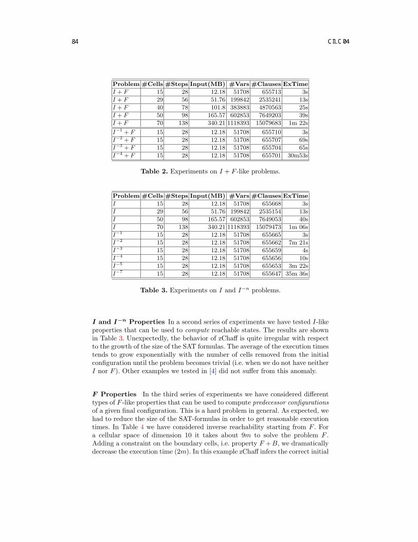
Problem #Cells #Steps Input(MB) #Vars #Clauses ExTime

I + F 15 28 12.18 51708 655713 3s

I + F 29 56 51.76 199842 2535241 13s

I + F 40 78 101.8 383883 4870563 25s

I + F 50 98 165.57 602853 7649203 39s

I + F 70 138 340.21 1118393 15079683 1m 22s

I−1 + F 15 28 12.18 51708 655710 3s

I−2 + F 15 28 12.18 51708 655707 69s

I−3 + F 15 28 12.18 51708 655704 65s

I−4 + F 15 28 12.18 51708 655701 30m53s

Table 2. Experiments on I + F -like problems.

Problem #Cells #Steps Input(MB) #Vars #Clauses ExTime

I 15 28 12.18 51708 655668 3s

I 29 56 51.76 199842 2535154 13s

I 50 98 165.57 602853 7649053 40s

I 70 138 340.21 1118393 15079473 1m 06s

I−1 15 28 12.18 51708 655665 3s

I−2 15 28 12.18 51708 655662 7m 21s

I−3 15 28 12.18 51708 655659 4s

I−4 15 28 12.18 51708 655656 10s

I−5 15 28 12.18 51708 655653 3m 22s

I−7 15 28 12.18 51708 655647 35m 36s

Table 3. Experiments on I and I−n problems.

I and I−n Properties In a second series of experiments we have tested I-likeproperties that can be used to compute reachable states. The results are shownin Table 3. Unexpectedly, the behavior of zChaff is quite irregular with respectto the growth of the size of the SAT formulas. The average of the execution timestends to grow exponentially with the number of cells removed from the initialconfiguration until the problem becomes trivial (i.e. when we do not have neitherI nor F ). Other examples we tested in [4] did not suffer from this anomaly.

F Properties In the third series of experiments we have considered differenttypes of F -like properties that can be used to compute predecessor configurationsof a given final configuration. This is a hard problem in general. As expected, wehad to reduce the size of the SAT-formulas in order to get reasonable executiontimes. In Table 4 we have considered inverse reachability starting from F . Fora cellular space of dimension 10 it takes about 9m to solve the problem F .Adding a constraint on the boundary cells, i.e. property F +B, we dramaticallydecrease the execution time (2m). In this example zChaff infers the correct initial

Problem #Cells #Steps Input(MB) #Vars #Clauses ExTime

F 10 18 5 22173 281010 9m 40s

F + B 10 18 5 22173 281013 2m 27s

F + B + 2L 10 18 5 22173 296623 35s

10F + B 10 18 5 22173 281043 39s

400F + B 10 18 5 22173 292983 1m 50s

Table 4. Experiments on F -like problems.

Problem C.o.I. #Cells #Steps Input(MB) #Vars #Clauses ExTime

F 1 + B 10 18 5 22173 280987 1m 48s

F 1 + B√

10 18 4 16773 241961 1m 59s

F 1 + B + 10L 10 18 5 22173 296605 2m 05s

F 1 + B + 10L√

10 18 4 16773 257561 1m 40s

F 1 + B + 30L 10 18 5 22173 330962 54s

F 1 + B + 30L√

10 18 4 16773 288791 59s

100F 1 + B 10 18 4 22173 281283 2m20s

100F 1 + B√

10 18 4 16773 241961 2m

C.o.I.=Reduction of the SAT-formula via the Cone of Influence

Table 5. Experiments on F 1-like problems.

configuration. The execution time further improves when forcing zChaff to selectthe variables occurring in F with the trick discussed at the beginning of thissection. Specifically, when duplicating the last step of the formula EvA zChafftakes 35s to solve the same problem (see prop. F + B + 2L in Table 4). Similarresults are obtained by simply copying F 10 times in the input formula given tozChaff (see prop. 10F + B in Table 4). Tuning the heuristics might be difficult(without modifying the code of zChaff) as shown by further experiments (like100F + B) where the performance gets worse again.

F 1 Properties In order to study the effectiveness of the cone of influencereduction we have also considered F−1 + B properties as shown in Table 5. Theuse of this reduction alone does not improve the execution time much (see F 1+Bwith and without C.o.I. in Table 5). However, when coupled with the n-copy ofthe last step of EvA (to force the selection of variables in F ) then it seems towork (see F 1+B+10L with and without C.o.I. in Table 5). Copying the formulaF does not seem to work well in this examples. Again tuning the parametersused in heuristic like the number of copies n in . . . + nL might be difficult bysimply using zChaff as a black box.

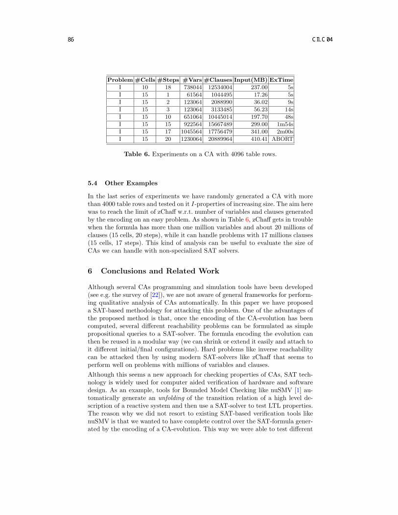
Problem #Cells #Steps #Vars #Clauses Input(MB) ExTime

I 10 18 738044 12534004 237.00 5s

I 15 1 61564 1044495 17.26 5s

I 15 2 123064 2088990 36.02 9s

I 15 3 123064 3133485 56.23 14s

I 15 10 651064 10445014 197.70 48s

I 15 15 922564 15667489 299.00 1m54s

I 15 17 1045564 17756479 341.00 2m00s

I 15 20 1230064 20889964 410.41 ABORT

Table 6. Experiments on a CA with 4096 table rows.

5.4 Other Examples

In the last series of experiments we have randomly generated a CA with morethan 4000 table rows and tested on it I-properties of increasing size. The aim herewas to reach the limit of zChaff w.r.t. number of variables and clauses generatedby the encoding on an easy problem. As shown in Table 6, zChaff gets in troublewhen the formula has more than one million variables and about 20 millions ofclauses (15 cells, 20 steps), while it can handle problems with 17 millions clauses(15 cells, 17 steps). This kind of analysis can be useful to evaluate the size ofCAs we can handle with non-specialized SAT solvers.

6 Conclusions and Related Work

Although several CAs programming and simulation tools have been developed(see e.g. the survey of [22]), we are not aware of general frameworks for perform-ing qualitative analysis of CAs automatically. In this paper we have proposeda SAT-based methodology for attacking this problem. One of the advantages ofthe proposed method is that, once the encoding of the CA-evolution has beencomputed, several different reachability problems can be formulated as simplepropositional queries to a SAT-solver. The formula encoding the evolution canthen be reused in a modular way (we can shrink or extend it easily and attach toit different initial/final configurations). Hard problems like inverse reachabilitycan be attacked then by using modern SAT-solvers like zChaff that seems toperform well on problems with millions of variables and clauses.Although this seems a new approach for checking properties of CAs, SAT tech-nology is widely used for computer aided verification of hardware and softwaredesign. As an example, tools for Bounded Model Checking like nuSMV [1] au-tomatically generate an unfolding of the transition relation of a high level de-scription of a reactive system and then use a SAT-solver to test LTL properties.The reason why we did not resort to existing SAT-based verification tools likenuSMV is that we wanted to have complete control over the SAT-formula gener-ated by the encoding of a CA-evolution. This way we were able to test different

kind of properties and heuristics on zChaff directly.In our preliminary experiments we have obtained interesting results for CAs ofreasonable size (e.g. 70 cells, 140 steps, 120 rules). We believe that it mightbe possible to manage larger problems by a specialization of the SAT-solvingalgorithm (and, especially, of its heuristics) that could benefit from structuralproperties of CAs. This might be an interesting future direction for our research.

References

1. A. Biere, E.M. Clarke, R. Raimi, Y. Zhu. Verifiying Safety Properties of a PowerPC Microprocessor Using Symbolic Model Checking without BDDs, CAV ’99, Lec-ture Notes in Computer Science, 60-71, 1999.

2. E. Burks. Essays on Cellular Automata, University of Illinois Press, 1972.3. E.F.Codd. Cellular Automata, Academic Press, New York, 1968.4. M. D’Antonio. Analisi SAT-based di Automi Cellulari, Tesi di laurea, Dip. di In-

formatica e Scienze dell’Informazione, Universita di Genova, Marzo 2004.5. M. Davis, H. Putnam. A computing procedure for quantification theory, Journal of

the Association for Computing Machinery, 1960.6. F. Green. NP-Complete Problems in Cellular Automata, Complex Systems, 1:453-

474, 1987.7. J. Groote, J. Warners The propositional formula checker HeerHugo, Journal of

Automated Reasoning, 24(1-2):101-125, 2000.8. The ICS home page: http://www.icansolve.com9. J. Kari. Cryptosystems based on reversible cellular automata, Preprint, 1992.

10. J. Kari. Reversability of 2D cellular automata is undecidable, Physica, Vol. D45:379-385, 1990.

11. C. Langton. Studying artificial life with cellular automata, Physica D, 22:120-140,1986.

12. J. Mazoyer. A six-state minimal time solution to the firing squad synchronizationproblem, Theoretical Computer Science, 50(2):183-240, Elsevier, 1987.

13. E.F. Moore. Sequential machines in: E.F. Moore Selected Papers, Addison-Wesley,Reading, 1964.

14. M.W. Moskewicz, C.F. Madigan, Y. Zhao, L. Zhang, S. Malik. Chaff: Engineeringan Efficient SAT Solver, Proceedings of the 38th Design Automation Conference(DAC’01), 2001.

15. D. A. Plaisted and S. Greenbaum. A Structure Preserving Clause Form Transla-tion. Journal of Symbolic Computation, 2(3):293–304, 1986.

16. The SIMO web page: http://www.mrg.dist.unige.it/ sim/simo/17. K. Sutner. On the computational complexity of finite cellular automata, JCSS,

50(1):87-97, 1995.18. J. von Neumann. Theory of Self-Reproducing Automata, University of Illinois Press,

edito e completato da A.W. Burks, 1966.19. S. Wolfram. Universality and complexity in cellular automata, Physica D, 10:1-35,

1984.20. S. Wolfram.Computation Theory of Cellular Automata, Communications in Math-

ematical Physics, 96:15-57, November 1984.21. S. Wolfram. Theory and Applications of Cellular Automata, World Scientific, 1986.22. T. Worsch. Programming Environments for Cellular Automata,Technical report

37/96, Universitat Karlsruhe, Fakultat fur Informatik, 1996.

Uniform relational frameworksfor modal inferences?

A. Formisano1, E. G. Omodeo1, E. S. Or lowska2, and A. Policriti3

1 Dip. di Informatica, Univ. dell’Aquila. formisano|omodeo@di.univaq.it2 Instytut Lacznosci, Warsaw, Poland. orlowska@itl.waw.pl

3 Dip. di Matematica e Informatica, Univ. di Udine. policriti@dimi.uniud.it

Abstract. The design and the implementation of variable-free deduc-tive frameworks (ultimately based on Tarski’s arithmetic of dyadic rela-tions) for aggregate theories, strongly rely on the availability of suitablepairing notions.Thanks to a set-theoretical treatment of modalities, we show that even inthe case of modal propositional logics, an appropriate pairing notion canbe introduced and exploited in order to devise an alternative approachto modal deduction.

Key words: Modal logic, relational systems, translation methods.

Introduction

In this paper we focus on a technical issue which plays a crucial role in algebraicformalization of set theory. The kind of formalization we have in mind sproutsfrom the historical line of work presented in the monograph [17]; but our con-tribution is much more specific, as it links with previous work on set-theoreticrenderings of non-classical logics, and such renderings only presuppose very weakaxioms concerning sets. It has been shown, in fact (cf. the box-as-powerset, inbrief -as-P, translation of [4, 1]), that even a very weak theory can offer ade-quate means for expressing the semantics of modal systems of propositional logic,for investigating the issue of their first-order representability, and for automatinginferences in non-classical contexts (cf. [10, pp. 478–481]). Unlike previous stud-ies, where suitable weak set theories were formalized within ordinary quantifiedcalculus (in one case, namely [14], an inferential system a la Rasiowa-Sikorskiwas developed), here we provide a variable-free, equational version of the targetset-theoretic language. To compensate for the lack of variables and quantifiers,the equality construct will be used for comparing expressions designating globalrelations between sets rather than for comparing set-expressions.

Providing a suitable notion of pairing is the central issue of the proposalwe put forward; in fact, pairing will be a key tool for obtaining, with minimalaxiomatic commitment, the desired equational support for the said set-rendering? This research benefited from collaborations fostered by the European action COST

n.274 (TARSKI, see http://www.tarski.org).

of modal logics specified a la Hilbert. Such a tool enables use of the Maddux-Monk-Tarski algorithm (cf. [17]) for restating any first-order sentence in threevariables; so it paves the way to the equational treatment of non-classical logics.As the present paper will illustrate through various examples stemming from thegeneral approach discussed in [2], the proposed pairing device can be built intoa specialized variant of the -as-P translation so as to drive it into a completelyequational setting.

An opportunity for improvements would have been missed if we had simplyproposed a montage of the -as-P translation with Maddux’ translation. Tomention one thing, the first-order sentences resulting from -as-P constitute arather narrow sublanguage of first-order logic, whose 3-variable translation caneasily be obtained by more direct means than by the general method. Moreover,in view of the special purpose of our translation, the first-order (set-theoretic)equivalent of a modal proposition can be left understood, and the two logicalphases of the overall translation can be fused into a single process. The roleof Maddux’ translation, in this process, can be superseded by the graph-basedapproach developed in [2], whose techniques, however, are conservative and donot guarantee success in all circumstances; therefore, suitable extensions of thatapproach had to be devised to take full advantage of the special context ofour discourse, where most of the relations entering into play are functions, andwhere conjugated projections (left and right inverses of the pairing function) areavailable.

As for the pairing function, none seems to be available under the very weakassumptions of the target set theory as originally proposed in [4, 1]. We musteither add an explicit pair axiom, or design a suitable variant of the P operation(cf. Sec.1): in either case, a well-known device due to Kuratowski (wherebyordered pairs can be encoded in terms of nested unordered pairs) can be adopted.

This paper is ‘twin’, in a sense, of [14]. Both develop a theory-based ap-proach, whose difference relative to a more typical calculus-based approach willbe sketched in Sec.3. Suffice it to say, for the time being, that, typically, oneassumes the universe of discourse to consist exclusively of the possible worlds ofa frame; here, instead, the universe of discourse results from the amalgamationof all Kripkean frames and hence encompasses worlds and frames together (aswell as other less relevant entities), all uniformly viewed as ‘sets’. Under one im-portant aspect this paper and [14] diverge, though: the Rasiowa-Sikorski systemadopted there is particularly handy and human-oriented, whereas the equationalkind of reasoning to which modal logics are reduced in this paper is intended tobe mainly oriented to machine formula-crunching.

1 Background axiomatic aggregate theory

Consider the axiomatic theory Ω whose postulates are

∀ y ∀x ∃n ∀ v(v ∈ n ↔ (v ∈ x & v ∈ y)

),

∀ y ∀x ∃ d ∀ v(v ∈ d ↔ ¬ (v ∈ x↔ v ∈ y)

),

∀x ∃ p ∀ v(v ∈ p ↔ (∀u ∈ v)(u ∈ x)

).

2

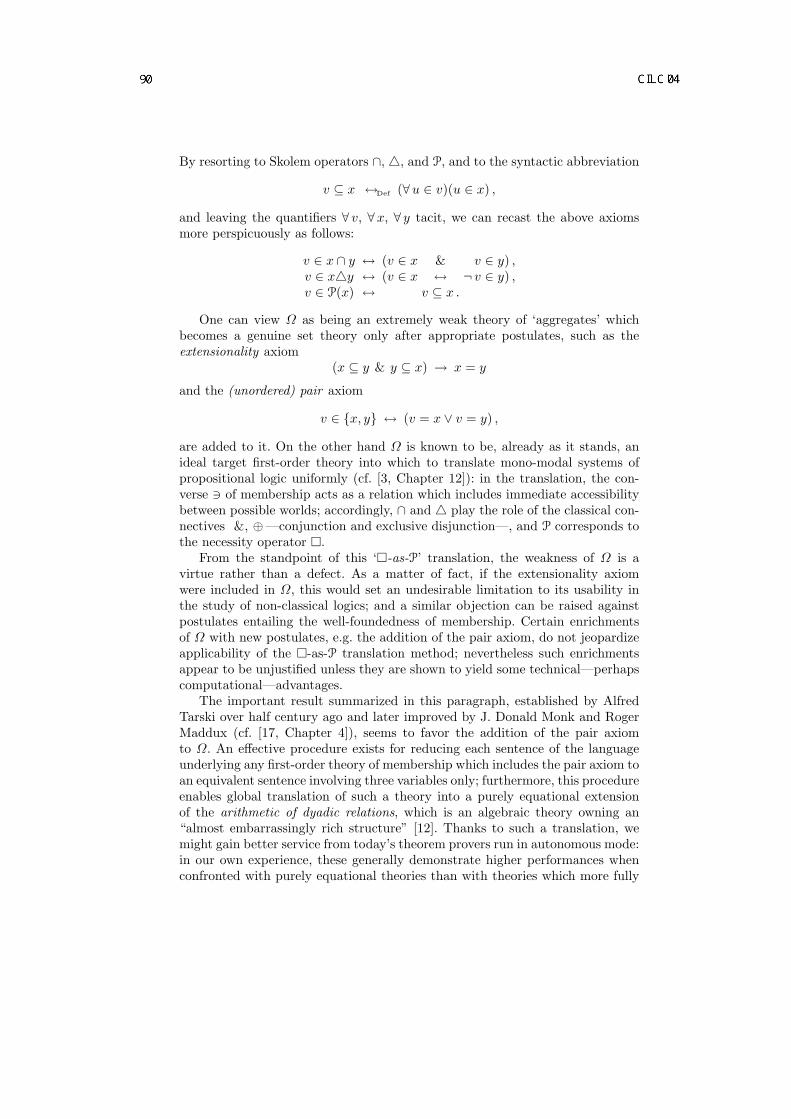
By resorting to Skolem operators ∩, 4, and P, and to the syntactic abbreviation

v ⊆ x ↔Def (∀u ∈ v)(u ∈ x) ,

and leaving the quantifiers ∀ v, ∀x, ∀ y tacit, we can recast the above axiomsmore perspicuously as follows:

v ∈ x ∩ y ↔ (v ∈ x & v ∈ y) ,v ∈ x4y ↔ (v ∈ x ↔ ¬ v ∈ y) ,v ∈ P(x) ↔ v ⊆ x .

One can view Ω as being an extremely weak theory of ‘aggregates’ whichbecomes a genuine set theory only after appropriate postulates, such as theextensionality axiom

(x ⊆ y & y ⊆ x) → x = y

and the (unordered) pair axiom

v ∈ x, y ↔ (v = x ∨ v = y) ,

are added to it. On the other hand Ω is known to be, already as it stands, anideal target first-order theory into which to translate mono-modal systems ofpropositional logic uniformly (cf. [3, Chapter 12]): in the translation, the con-verse 3 of membership acts as a relation which includes immediate accessibilitybetween possible worlds; accordingly, ∩ and 4 play the role of the classical con-nectives &, ⊕—conjunction and exclusive disjunction—, and P corresponds tothe necessity operator .

From the standpoint of this ‘-as-P’ translation, the weakness of Ω is avirtue rather than a defect. As a matter of fact, if the extensionality axiomwere included in Ω, this would set an undesirable limitation to its usability inthe study of non-classical logics; and a similar objection can be raised againstpostulates entailing the well-foundedness of membership. Certain enrichmentsof Ω with new postulates, e.g. the addition of the pair axiom, do not jeopardizeapplicability of the -as-P translation method; nevertheless such enrichmentsappear to be unjustified unless they are shown to yield some technical—perhapscomputational—advantages.

The important result summarized in this paragraph, established by AlfredTarski over half century ago and later improved by J. Donald Monk and RogerMaddux (cf. [17, Chapter 4]), seems to favor the addition of the pair axiomto Ω. An effective procedure exists for reducing each sentence of the languageunderlying any first-order theory of membership which includes the pair axiom toan equivalent sentence involving three variables only; furthermore, this procedureenables global translation of such a theory into a purely equational extensionof the arithmetic of dyadic relations, which is an algebraic theory owning an“almost embarrassingly rich structure” [12]. Thanks to such a translation, wemight gain better service from today’s theorem provers run in autonomous mode:in our own experience, these generally demonstrate higher performances whenconfronted with purely equational theories than with theories which more fully

3

exploit the symbolic first-order apparatus [8, 9]. By translating modal axiomsand theses into an equational variant of Ω, we could hence best benefit of currentproof technology.

We will propose below an even less committing way of reducing (a variantΩ′ of) Ω to the arithmetic of relations, taking advantage of the fact that theabove cited Tarski-Maddux’ result holds also for theories where an analogue ofthe pair axiom, of the form

∀ y ∀x ∃ q ∀ v(v in q ↔ (v = x ∨ v = y)

),

can be derived from the axioms. The only requirement, in regard to this, is that“v in q” be a formula which involves three variables altogether and has v andq as its sole free variables. To achieve our translation purpose, we just have toretouch the one axiom which characterizes the ‘powerset’ operator P so that itbehaves more naturally when the extensionality axiom is missing. Our proposedreplacement for the third axiom of Ω is the sentence

∀x ∃ p ∀ v(v ∈ p ↔ (v = x ∨ v ⊂ x)

),

where

v ⊂ x ↔Def ¬ (v ⊆ x→ x ⊆ v)

(that is, v ⊂ x holds if and only if every element of v belongs to x whereas xhas some element not belonging to v). Under this revised axiom, even withoutextensionality axiom, it is clear that exactly one p, let us call it P(x), correspondsto each x so that the elements of p are precisely x and all of its strict subsetsv ⊂ x. Likewise, to any q there corresponds at most one a such that q max aholds, where

q max a ↔Def

(a ∈ q & q ⊆ P(a)

);

but, unlike P which is total, max is a partial function of its first operand.In our revised version Ω′ of Ω, one can conceive an analogue of the unordered

pair a, b to be P(a) when a = b and to have the same elements as P(a)4P(b)when a 6= b. (Out of such ‘unordered pairs’, one can proceed to construct ‘orderedpairs’ analogous to Kazimierz Kuratowski’s pairs 〈a, b〉 =Def

a, b, a, a

, and

these will behave as desired, but let us avoid a discussion on this point takingit for granted [6].) With this rationale in mind, we can characterize as followsa ‘pseudo-membership’ which meets the formal analogue seen above of the pairaxiom:

b in q ↔Def

(b ∈ q &

(¬∃ d ∈ q

)(b ⊂ d

))∨ ∃ a

(q max a & b ⊂ a

& ∀ d(d ∈ q↔

(d ∈ P(a) & ¬ d ∈ P(b)

))).

To see that in can be specified in three variables, it suffices to observe that since

4

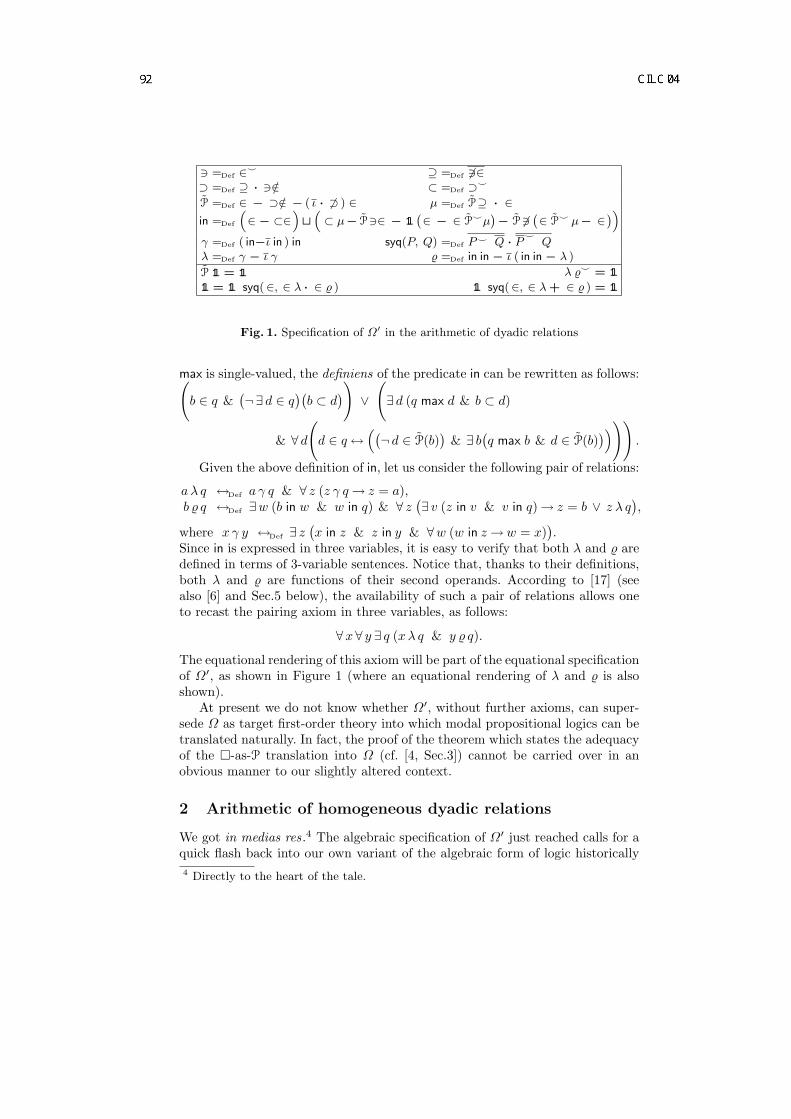
3 =Def ∈^ ⊇ =Def 63∈⊃ =Def ⊇ · 3/∈ ⊂ =Def ⊃^

P =Def ∈ − ⊃/∈ − ( ι · 6⊃ ) ∈ µ =Def P⊇ · ∈in =Def

“∈ − ⊂∈

”t

“⊂ µ − P3∈ − 1l

`∈ − ∈ P^µ

´− P 63

`∈ P^ µ − ∈

´”γ =Def ( in−ι in ) in syq(P, Q) =Def P ^ Q · P

^Q

λ =Def γ − ι γ % =Def in in − ι ( in in − λ )

P 1l = 1l λ %^ = 1l

1l = 1l syq(∈, ∈ λ · ∈ % ) 1l syq(∈, ∈ λ + ∈ % ) = 1l

Fig. 1. Specification of Ω′ in the arithmetic of dyadic relations

max is single-valued, the definiens of the predicate in can be rewritten as follows:(b ∈ q &

(¬∃ d ∈ q

)(b ⊂ d

))∨

(∃ d (q max d & b ⊂ d)

& ∀ d

(d ∈ q↔

((¬ d ∈ P(b)

)& ∃ b

(q max b & d ∈ P(b)

)))).

Given the above definition of in, let us consider the following pair of relations:

aλ q ↔Def a γ q & ∀ z (z γ q→ z = a),b % q ↔Def ∃w (b in w & w in q) & ∀ z

(∃ v (z in v & v in q)→ z = b ∨ z λ q

),

where x γ y ↔Def ∃ z(x in z & z in y & ∀w (w in z→ w = x)

).

Since in is expressed in three variables, it is easy to verify that both λ and % aredefined in terms of 3-variable sentences. Notice that, thanks to their definitions,both λ and % are functions of their second operands. According to [17] (seealso [6] and Sec.5 below), the availability of such a pair of relations allows oneto recast the pairing axiom in three variables, as follows:

∀x∀ y ∃ q (xλ q & y % q).

The equational rendering of this axiom will be part of the equational specificationof Ω′, as shown in Figure 1 (where an equational rendering of λ and % is alsoshown).

At present we do not know whether Ω′, without further axioms, can super-sede Ω as target first-order theory into which modal propositional logics can betranslated naturally. In fact, the proof of the theorem which states the adequacyof the -as-P translation into Ω (cf. [4, Sec.3]) cannot be carried over in anobvious manner to our slightly altered context.

2 Arithmetic of homogeneous dyadic relations

We got in medias res.4 The algebraic specification of Ω′ just reached calls for aquick flash back into our own variant of the algebraic form of logic historically4 Directly to the heart of the tale.

5

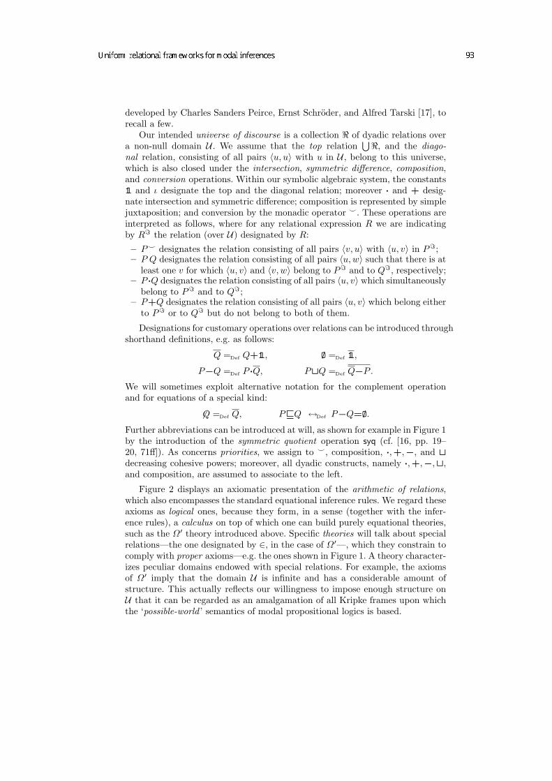
developed by Charles Sanders Peirce, Ernst Schroder, and Alfred Tarski [17], torecall a few.

Our intended universe of discourse is a collection < of dyadic relations overa non-null domain U . We assume that the top relation

⋃<, and the diago-

nal relation, consisting of all pairs 〈u, u〉 with u in U , belong to this universe,which is also closed under the intersection, symmetric difference, composition,and conversion operations. Within our symbolic algebraic system, the constants1l and ι designate the top and the diagonal relation; moreover · and + desig-nate intersection and symmetric difference; composition is represented by simplejuxtaposition; and conversion by the monadic operator ^. These operations areinterpreted as follows, where for any relational expression R we are indicatingby R= the relation (over U) designated by R:

– P^ designates the relation consisting of all pairs 〈v, u〉 with 〈u, v〉 in P=;– P Q designates the relation consisting of all pairs 〈u,w〉 such that there is at

least one v for which 〈u, v〉 and 〈v, w〉 belong to P= and to Q=, respectively;– P ·Q designates the relation consisting of all pairs 〈u, v〉 which simultaneously

belong to P= and to Q=;– P+Q designates the relation consisting of all pairs 〈u, v〉 which belong either

to P= or to Q= but do not belong to both of them.

Designations for customary operations over relations can be introduced throughshorthand definitions, e.g. as follows:

Q =Def Q+1l, Ø =Def 1l,

P−Q =Def P ·Q, PtQ =Def Q−P .We will sometimes exploit alternative notation for the complement operationand for equations of a special kind:

6Q =Def Q, PvQ ↔Def P−Q=Ø.

Further abbreviations can be introduced at will, as shown for example in Figure 1by the introduction of the symmetric quotient operation syq (cf. [16, pp. 19–20, 71ff]). As concerns priorities, we assign to ^, composition, ·,+,−, and tdecreasing cohesive powers; moreover, all dyadic constructs, namely ·,+,−,t,and composition, are assumed to associate to the left.

Figure 2 displays an axiomatic presentation of the arithmetic of relations,which also encompasses the standard equational inference rules. We regard theseaxioms as logical ones, because they form, in a sense (together with the infer-ence rules), a calculus on top of which one can build purely equational theories,such as the Ω′ theory introduced above. Specific theories will talk about specialrelations—the one designated by ∈, in the case of Ω′—, which they constrain tocomply with proper axioms—e.g. the ones shown in Figure 1. A theory character-izes peculiar domains endowed with special relations. For example, the axiomsof Ω′ imply that the domain U is infinite and has a considerable amount ofstructure. This actually reflects our willingness to impose enough structure onU that it can be regarded as an amalgamation of all Kripke frames upon whichthe ‘possible-world ’ semantics of modal propositional logics is based.

6

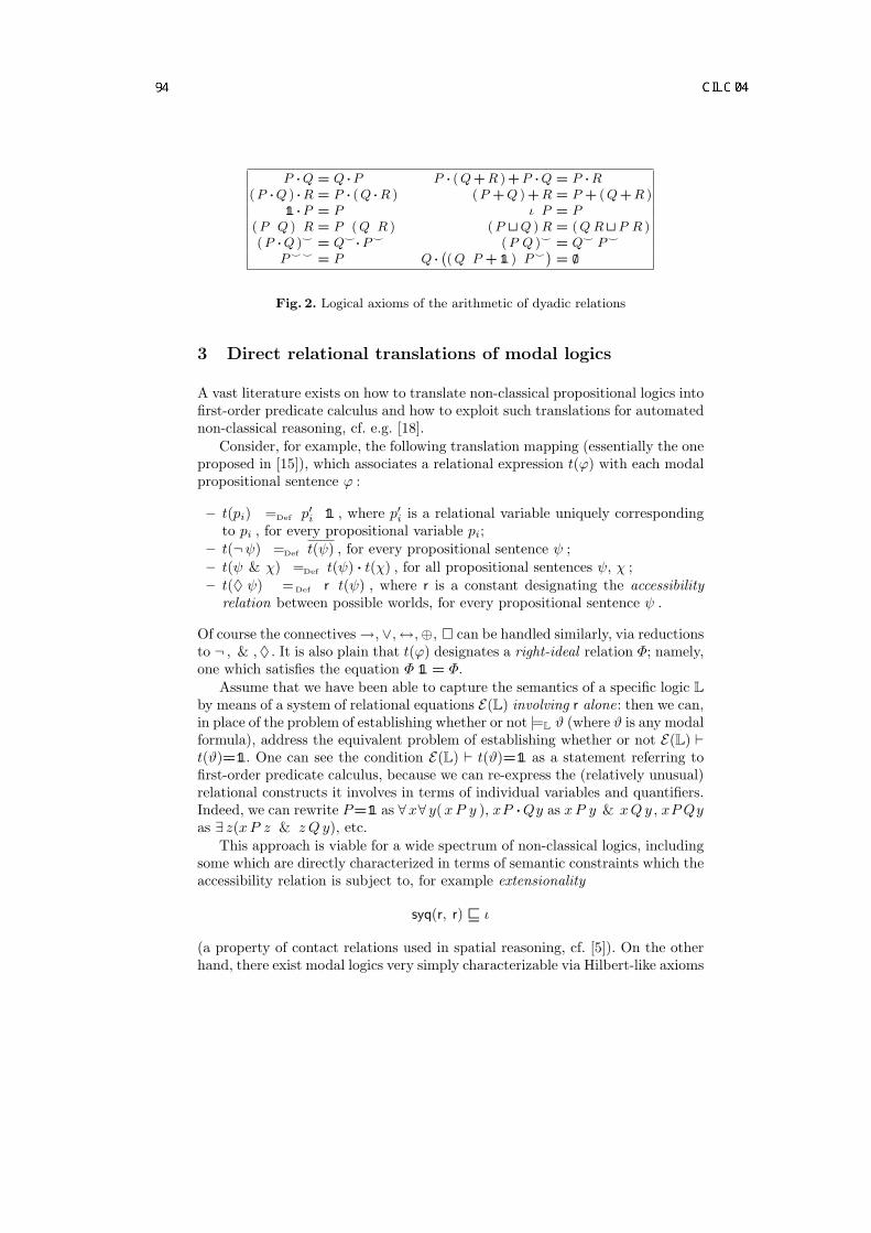
P · Q = Q · P P · ( Q+R ) +P · Q = P · R( P · Q ) · R = P · ( Q · R ) ( P +Q ) +R = P + ( Q+R )

1l · P = P ι P = P( P Q ) R = P ( Q R ) ( P t Q ) R = ( Q R t P R )( P · Q )^ = Q^· P ^ ( P Q )^ = Q^ P ^

P ^^ = P Q ·`( Q P + 1l ) P ^

´= Ø

Fig. 2. Logical axioms of the arithmetic of dyadic relations

3 Direct relational translations of modal logics

A vast literature exists on how to translate non-classical propositional logics intofirst-order predicate calculus and how to exploit such translations for automatednon-classical reasoning, cf. e.g. [18].

Consider, for example, the following translation mapping (essentially the oneproposed in [15]), which associates a relational expression t(ϕ) with each modalpropositional sentence ϕ :

– t(pi) =Def p′i 1l , where p′i is a relational variable uniquely correspondingto pi , for every propositional variable pi;

– t(¬ψ) =Def t(ψ) , for every propositional sentence ψ ;– t(ψ & χ) =Def t(ψ) · t(χ) , for all propositional sentences ψ, χ ;– t(♦ ψ) =Def r t(ψ) , where r is a constant designating the accessibility

relation between possible worlds, for every propositional sentence ψ .

Of course the connectives →,∨,↔,⊕, can be handled similarly, via reductionsto ¬ , & ,♦ . It is also plain that t(ϕ) designates a right-ideal relation Φ; namely,one which satisfies the equation Φ 1l = Φ.

Assume that we have been able to capture the semantics of a specific logic Lby means of a system of relational equations E(L) involving r alone: then we can,in place of the problem of establishing whether or not |=L ϑ (where ϑ is any modalformula), address the equivalent problem of establishing whether or not E(L) `t(ϑ)=1l. One can see the condition E(L) ` t(ϑ)=1l as a statement referring tofirst-order predicate calculus, because we can re-express the (relatively unusual)relational constructs it involves in terms of individual variables and quantifiers.Indeed, we can rewrite P=1l as ∀x∀ y(xP y ), xP ·Qy as xP y & xQy , xP Qyas ∃ z(xP z & z Qy), etc.

This approach is viable for a wide spectrum of non-classical logics, includingsome which are directly characterized in terms of semantic constraints which theaccessibility relation is subject to, for example extensionality

syq(r, r) v ι

(a property of contact relations used in spatial reasoning, cf. [5]). On the otherhand, there exist modal logics very simply characterizable via Hilbert-like axioms

7

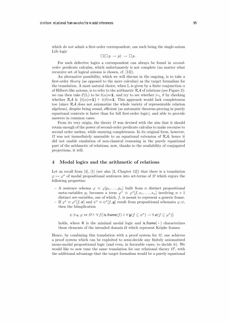
which do not admit a first-order correspondent, one such being the single-axiomLob logic

( p → p) → p .

For such defective logics a correspondent can always be found in second-order predicate calculus, which unfortunately is not complete (no matter whatrecursive set of logical axioms is chosen, cf. [13]).

An alternative possibility, which we will discuss in the ongoing, is to take afirst-order theory (as opposed to the mere calculus) as the target formalism forthe translation. A most natural choice, when L is given by a finite conjunction αof Hilbert-like axioms, is to refer to the arithmetic RA of relations (see Figure 2):we can then take E(L) to be t(α)=1l, and try to see whether |=L ϑ by checkingwhether RA &

(t(α)=1l

)` t(ϑ)=1l. This approach would lack completeness

too (since RA does not axiomatize the whole variety of representable relationalgebras), despite being sound, efficient (as automatic theorem-proving in purelyequational contexts is faster than for full first-order logic), and able to provideanswers in common cases.

From its very origin, the theory Ω was devised with the aim that it shouldretain enough of the power of second-order predicate calculus to make recourse tosecond order useless, while ensuring completeness. In its original form, however,Ω was not immediately amenable to an equational extension of RA; hence itdid not enable emulation of non-classical reasoning in the purely equationalpart of the arithmetic of relations; now, thanks to the availability of conjugatedprojections, it will.

4 Modal logics and the arithmetic of relations

Let us recall from [4], [1] (see also [3, Chapter 12]) that there is a translationϕ 7→ ϕ? of modal propositional sentences into set-terms of Ω which enjoys thefollowing properties:

– A sentence schema ϕ ≡ ϕ[p1, . . . , pn] built from n distinct propositionalmeta-variables pi becomes a term ϕ? ≡ ϕ?[f, x1, . . . , xn] involving n + 1distinct set-variables, one of which, f , is meant to represent a generic frame.

– If ϕ? ≡ ϕ?[f,x] and ψ? ≡ ψ?[f,y] result from propositional schemata ϕ,ψ,then the biimplication

ψ |=K ϕ⇔ Ω ` ∀ f(is frame(f) ∧ ∀y(f ⊆ ψ?) → ∀x(f ⊆ ϕ?)

)holds, where K is the minimal modal logic and is frame( · ) characterizesthose elements of the intended domain U which represent Kripke frames.

Hence, by combining this translation with a proof system for Ω, one achievesa proof system which can be exploited to semi-decide any finitely axiomatizedmono-modal propositional logic (and even, in favorable cases, to decide it). Wewould like to now tune the same translation for our relational theory Ω′, withthe additional advantage that the target formalism would be a purely equational

8

one in the case at hand; however, due to the difficulty mentioned at the end ofSec.1, in the rest of this paper we replace Ω′ by the (equational) theory Ω′′

consisting of the axioms of Ω′ plus the axiom

P 1l = 1l, where P =Def syq(⊆, ∈) and ⊆ =Def 3/∈ .

We begin by specifying the monadic relation is frame, bearing in mind thatsince 3 must act, when restricted to a frame, as the accessibility relation betweenworlds in that frame, a frame f must be a transitive set, i.e., it must satisfyf ⊆ P(f). This characterization turns out to be adequate to our purposes:

is frame =Def ι · P ⊇ .

Then we must specify operations on U that correspond to the propositionalconstructs ∨ , & , and . Here the rationale is that the term ϕ[f,x] into whichone translates a propositional schema ϕ?[p] represents the collection of all worlds(in the frame f) where ϕ holds. We have announced already in Sec.1 that thenatural counterparts of and & will be P and ∩: analogously, ∪ and \ willact as counterparts of ∨ and 6→ , but since we have not introduced any of ∩, ∪,and \ explicitly in Figure 1, we can fill this gap now by putting5

∩ =Def syq(∈, ∈ λ · ∈ % ) , ∪ =Def syq(∈, ∈ λt ∈ % ) ,\ =Def syq(∈, ∈ λ− ∈ % ) .

In the language underlying the Skolemized first-order version of Ω′′, it is quitestraightforward to define the mapping ϕ[p] 7→ ϕ?[f,x] of sentence schemata intoterms:

p?i =Def xi , (¬ψ)? =Def f \ ψ? ,

(ψ→ χ)? =Def (¬ψ)? ∪ χ? , ( ψ)? =Def P(ψ?) .

(of course we can also handle the connectives & , ∨ , ↔ , ⊕ ,♦ via reductions to¬ , → ,). This is called the -as-P translation. Assuming that we manage tospecify the relation f 6⊆ ϕ?[f,x] between a frame f and a tuple x by means ofa relational expression ϕ, then the translation of Ψ `K ϕ (where Ψ stands for afinite collection of sentence schemata) into a derivability problem regarding the(quantifier-free, purely equational) relational version of Ω′′ will be

Ω′′ ` is frame · ϕ 1l v &Ψ 1l .

5 Compliance of a frame with a modal schema

How can we specify algebraically the relation (complement of the ϕ just intro-duced) which holds between a frame f and a tuple x when f ⊆ ϕ?[f,x]? A

5 Needless to say, we must distinguish between ·,+, −, t, v, which operate on rela-tions, and corresponding constructs ∩,4, \,∪,⊆, which operate on U .

9

crucial observation is that within the relational version of Ω′′ one can deriveequations

L^ L v ι , R^ R v ι , L^ R = 1l , ι v L 1lR^ ,

for suitably chosen relational expressions L,R. For example, we can take

L =Def λ^ t (ι−λ^ 1l) , R =Def %

^ t (ι− %^ 1l) .

This remark immediately discloses the possibility of translating the full-fledgedlanguage of first-order Ω′′ into the language of the arithmetic of relations: we canrely, for that, on a fundamental algorithm due to R. Maddux and explained in[17, Sec. 4.4]. Notice that the very fact that we can speak of tuples belonging toU relies on the availability of L,R. As a matter of fact, we can view each elementa of U as a pair 〈b, c〉 whose components fulfill aL=b and aR=c; accordingly, sincewe can decompose c in the same fashion, any element of U encodes a tuple ofany desired length. On the other hand, L^R = 1l implies that we can assemblea pair 〈b, c〉 from any two elements b, c of U , and hence we can form an n-tuplewith given components b1, . . . , bn for any finite number n.

We are not so much interested in translating the full first-order language intothe equational one as we are in translating formulas f ⊆ ϕ?[f,x]: these are, infact, the ones we really need in order to carry out the translation of any sentenceof modal propositional logic into relational Ω′′. To this end, we can resort to amore direct graph-based translation approach explained in [2], which has beenimplemented by means of a tool for algebraic graph transformation named Agg(acronym for ‘Attribute Graph Grammars’), developed at the TU, Berlin [11, 7].

Figure 3 displays the graph representation of f ⊆ ϕ?[f,x], when ϕ is one ofthe following modal sentences (x, y correspond to p and q, respectively):

S4: p → p;Lob: ( p → p) → p;K: (p → q) → ( p → q).

When fed with one of these three graphs, the thinning algorithm of [2, p. 455]terminates in a dead end. Figure 4 displays two of the resulting irreduciblegraphs, obscuring orientation and labels of the edges. Figures 5, 6, and 7 show, ona couple of examples, how to take advantage of the available ‘projections’ λ^, %^

to bring an irreducible graph to a form whence the thinning algorithm can resumeits job and terminate successfully, with the desired relational translation. (Noticethat, the last graph of Figure 7 can be further reduced as done for the examplein Figure 5.)

The key point is that, thanks to the availability of a pair of projections, λ^

and %^, the thinning algorithm can be enriched with a new graph-rewriting rule:

pair-encoding rule. Let L and R be a pair of conjugated projections. Letν′ and ν′′ be two nodes in a graph. Then introduce a new (bound) node νtogether with two labelled edges [ν, L, ν′] and [ν,R, ν′′].

10

ww wif w w ixw

⊇

∪ - λ

PY% 6

\?

λ - %

P- -

f ⊆ f \ P(x) ∪ P(P(x))

ww wif ww ww

wwix

w⊇

∪-λ

PY%

\

λ-P

∪*%

%

Y λY

\6

% -

λj

- -

f ⊆ f \ P(f \ P(x) ∪ x) ∪ P(x)

w www

www

wwww

www

w

wwwif x, y

-∪ -∪

-λ \

%

λ % P

% 9P

P

HHHY\HHHY

%

HHHjλHHHY

\

XXXXXXXXXy%

XXXXzλ HHj

% 6%

%

λ-

λ

-

⊇Kλ

-

∪

Y

--

f ⊆ f \ P(f \ x ∪ y) ∪ (f \ P(x)) ∪ P(y)

Fig. 3. Graph renderings of S4, Lob, and K

Such a rule is extremely general and, in principle, there is no restriction on itsapplicability. Clearly, it is convenient to exploit this rule within a strategy thatrelates its application to the firing of other rules of the thinning algorithm. Inparticular, since L and R are single-valued, the following rewriting-rule (cf. [2])becomes crucial in order to bring to end the graph-rewriting process:

functionality rule. Let [ν, P, ν′] be a labelled edge such that P is single-valued and let [ν′, Q, ν′′] be another edge, with ν 6= ν′′. Then the edge[ν′, Q, ν′′] is removed and the new edge [ν, P Q, ν′′] is added to the graph. (Ifthe graph contains another edge between ν and ν′′ labelled S, then a fusionis made and the new edge will be labelled P Q·S.)

Conclusions

In this paper we moved the first step toward the realization of an alternativedeductive framework for non-classical logics based on pure equational reasoning.

11

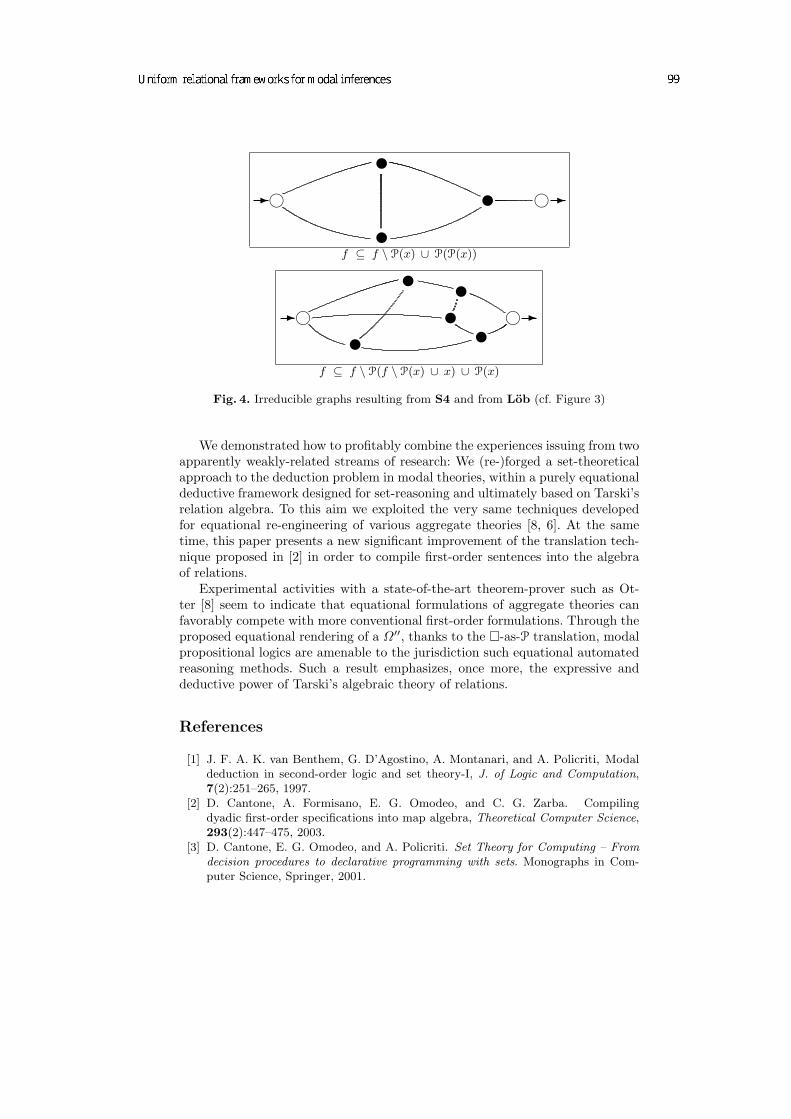
wi w i

w- -

f ⊆ f \ P(x) ∪ P(P(x))w wi ww w i- -

f ⊆ f \ P(f \ P(x) ∪ x) ∪ P(x)

Fig. 4. Irreducible graphs resulting from S4 and from Lob (cf. Figure 3)

We demonstrated how to profitably combine the experiences issuing from twoapparently weakly-related streams of research: We (re-)forged a set-theoreticalapproach to the deduction problem in modal theories, within a purely equationaldeductive framework designed for set-reasoning and ultimately based on Tarski’srelation algebra. To this aim we exploited the very same techniques developedfor equational re-engineering of various aggregate theories [8, 6]. At the sametime, this paper presents a new significant improvement of the translation tech-nique proposed in [2] in order to compile first-order sentences into the algebraof relations.

Experimental activities with a state-of-the-art theorem-prover such as Ot-ter [8] seem to indicate that equational formulations of aggregate theories canfavorably compete with more conventional first-order formulations. Through theproposed equational rendering of a Ω′′, thanks to the -as-P translation, modalpropositional logics are amenable to the jurisdiction such equational automatedreasoning methods. Such a result emphasizes, once more, the expressive anddeductive power of Tarski’s algebraic theory of relations.

References

[1] J. F. A. K. van Benthem, G. D’Agostino, A. Montanari, and A. Policriti, Modaldeduction in second-order logic and set theory-I, J. of Logic and Computation,7(2):251–265, 1997.

[2] D. Cantone, A. Formisano, E. G. Omodeo, and C. G. Zarba. Compilingdyadic first-order specifications into map algebra, Theoretical Computer Science,293(2):447–475, 2003.

[3] D. Cantone, E. G. Omodeo, and A. Policriti. Set Theory for Computing – Fromdecision procedures to declarative programming with sets. Monographs in Com-puter Science, Springer, 2001.

12

wi w i

w

-

-?

R

P Q

S

R

T

U- -

by applying the pair-encoding rule we obtain:wi w i

w

-

-?

R

P Q

S

R

T

Uw λ^

%^

R

- -

by applying functionality three times:wi w i

wR

Rw λ^

%^·λ^ R

R

P λ Q

S %T

U- -

Fig. 5. Rehabilitation of an irreducible graph (cf. the first graph in Figure 4)

[4] G. D’Agostino, A. Montanari, and A. Policriti, A set-theoretic translation methodfor polymodal logics, J. of Automated Reasoning, 3(15):317–337, 1995.

[5] I. Duntsch, E. Or lowska. A proof system for contact relation algebras, J. Philo-sophical Logic, 29:241-262, 2000.

[6] A. Formisano, E. G. Omodeo, and A. Policriti. Three-variable statements of set-pairing. Theoretical Computer Science (special issue in honor of Denis Richard,still to appear), 2004.

[7] A. Formisano, E. G. Omodeo, and M. Simeoni. A graphical approach to relationalreasoning. In W. Kahl, D. L. Parnas, and G. Schmidt Eds. Electronic Notes inTheoretical Computer Science, 44(3), Elsevier Science, 2003.

[8] A. Formisano, E. G. Omodeo, and M. Temperini. Layered map reasoning: Anexperimental approach put to trial on sets. In A. Dovier and M. C. Meo andA. Omicini Eds. Electronic Notes in Theoretical Computer Science, 48, ElsevierScience, 2001.

[9] A. Formisano, E. G. Omodeo, and M. Temperini. Instructing equational set-reasoning with Otter. In R. Gore and A. Leitsch and T. Nipkow Eds., AutomatedReasoning. Proc. of First International Joint Conference on Automated Reason-ing (IJCAR’01–(CADE+FTP+TABLEAUX), Siena), Lecture Notes in ComputerScience 2083, pp. 152-167, Springer, 2001.

[10] A. Formisano and A. Policriti. T -resolution: refinements and model elimination.J. of Automated Reasoning, 22(4):433–483, 1999.

[11] A. Formisano and M. Simeoni. An AGG application supporting visual reasoning.In L. Baresi and M. Pezze Eds. Electronic Notes in Theoretical Computer Science,50(3), Elsevier Science, 2001.

[12] P. R. Halmos. Algebraic Logic. Chelsea, New York, 1962.

13

Initial graph:

wh

wh

w

wwP1

P2

IP3

?

P4

6P5

-P6

i

P7*

P8

*

P9

?

P10 -

P11

-

- -

by applying the pair-encoding rule twice:

wh

wh

w

www wλ^

I

%^

%^

R

λ^

P1

P2

IP3

?

P4

6P5

-P6

i

P7*

P8

*

P9

?

P10 -

P11

-

- -

by applying functionality twice:

wh

wh

w

www wλ^

I

%^ %^R

λ^

P1

P2

IP3

?

P4

6P5

-P6

i

P7*

P8

*

P9

?

P10 -

Q1

-

Q1 =Def %^ P11 %

- -

Fig. 6. Rehabilitation of an irreducible graph (continued in Figure 7)

[13] L. Henkin. Completeness in the theory of types. In J. Hintikka ed., The philosophyof mathematics, Oxford readings in Philosophy, Oxford University Press, 1969,pp.51–63 (1950).

[14] E. Omodeo, E. S. Or lowska, and A. Policriti. Rasiowa-Sikorski style relationalelementary set theory. In R. Berghammer and B. Moeller Eds., Proc. 7th Inter-national Seminar on Relational Methods in Computer Science (RelMiCS’03, May12–17, 2003, Malente, Germany).

[15] E. S. Or lowska. Relational semantics for nonclassical logics: Formulas are rela-tions, In J. Wolenski ed., Philosophical Logic in Poland, pp. 167-186, 1994.

[16] G. Schmidt and T. Strohlein. Relations and Graphs –Discrete Mathematicsfor Computer Scientists. EATCS-Monographs on Theoretical Computer Science,Springer, 1993.

[17] A. Tarski and S. Givant. A formalization of set theory without variables, vol. 41of Colloquium Publications. American Mathematical Society, 1987.

14

by applying functionality twice:

wh

wh

w

www wλ^

I

Q2 Q3R

λ^

P1

P2

I

P5

-P6

i

P7*

P8

*

P9

?

P10 -

Q1

-

Q2 =Def %^·λ^ P3Q3 =Def %^·λ^ P ^

4

- -

by applying functionality twice:

wh

wh

w

www wλ^

I

Q2 Q3R

λ^

Q4

P2

I

Q5

* P6i

P7*

P8

*

P9

?

P10 -

Q1

-

Q4 =Def λ^ P1Q5 =Def λ^ P5

- -

by the usual thinning algorithm:

wh hw Q5

* P6i

Q3 P7*

P8

*

P9

?

Q6

-

Q6 =Def (Q^4 ·P ^

2 Q^2 ) (Q1·λ^ P10 λ)

- -

Fig. 7. Rehabilitation of an irreducible graph

[18] L. A. Wallen. Automated proof-search in non-classical logics – Efficient matrixproof methods for modal and intuitionistic logics, The MIT Press, Cambridge,MA, and London, 1990.

15

Constraint Based Protein Structure PredictionExploiting Secondary Structure Information

Alessandro Dal Palu2, Sebastian Will1, Rolf Backofen1, and Agostino Dovier2

1 Jena Center of Bioinformatics, Institute of Computer Science,Friedrich-Schiller-University, Jena. Ernst-Abbe-Platz 2, 07743 Jena (Germany).

2 Department of Mathematics and Computer Science, University of Udine. Via delleScienze 206, 33100 Udine (Italy).

Abstract. The protein structure prediction problem is one of the moststudied problems in Computational Biology. It can be reasonably ab-stracted as a minimization problem. The function to be minimized de-pends on the distances between the various amino-acids composing theprotein and on their types. Even with strong approximations, the prob-lem is shown to be computationally intractable. However, the solution ofthe problem for an arbitrary input size is not needed. Solutions for pro-teins of length 100–200 would give a strong contribution to Biotechnol-ogy. In this paper, we tackle the problem with constraint-based methods,using additional constraints and heuristics coming from the secondarystructure of a protein that can be quickly predicted with acceptable ap-proximation. Our prototypic implementation is written using constraintsover finite domains in the Mozart programming system. It improves overany previous constraint-based approach and shows the power and flexi-bility of the method. Especially, it is well suited for further extensions.

1 Introduction

A protein is identified by a finite list of amino-acids, which we can represent assymbols of an alphabet of 20 elements. The protein structure prediction (PSP)problem is the problem of predicting the 3D structure of the protein (its na-tive conformation) when the list of amino-acids is known. Native conformationdetermines the Biological function of the protein. It is accepted that the na-tive conformation is the state of minimum free energy. Up to now, though, adefinitive energy model has not been yet devised. The energy of a conforma-tion depends partially on the distances between all pairs of amino-acids and ontheir type. Thus, the PSP problem can be simplified to that of minimizing asuitable energy function generated by the protein 3D conformations. Althoughthe problem, even with some simplifications, is NP-complete [9], it deserves to beattacked, because a solution for ‘small’ proteins (100–200 amino-acids) would beanyhow extremely important in Biology and Biotechnology. The problem is ap-proached in several ways (see [7, 14] for a review). Prediction methods make useof statistical information available from more than 24, 000 structures depositedin the Protein Data Bank (PDB) [5]. The correct fold for a new sequence can beobtained when homology (sequence similarity) is detected with a sequence for

which the structure is available. Another approach tries to superimpose (thread)a chain on known structures and evaluates the plausibility of the fold.

Ab-initio methods, instead, try to find the native conformation without directreference to a structural model. In this context, a constraint-based encoding ofthe problem is extremely natural. A first abstraction is the choice of a spatialmodel for the admissible positions of the various amino-acids. Lattice models areused to formalize the PSP problem as a minimization problem on finite domains.It has been shown [4, 3, 12] that the Face-Centered-Cubic lattice (FCC) providesthe best lattice approximation of proteins. Moreover, it has been shown that theresidue neighbors in real proteins are clustered in a rather dense way, occupyingpositions closely approximating those of a distorted FCC packing. It is believedthat this packing is a direct manifestation of the hydrophobic effect. Recall thatFCC is the closest packing of spheres, which was proven only recently [8].

The FCC lattice is exploited in [1, 16] for solving proteins of length up to 160with the further abstraction of splitting the amino-acids in two families (H andP). However, the HP abstraction does not ensure that the result is the nativeconformation; in particular, the local sub-conformations of the form of α-helicesor β-strands (cf. Sect. 2) are often lost. These structures are often generated earlyin the real folding process and, moreover, the structures can be predicted withgood approximation [13]. These two observations suggest to include secondarystructures in the constraint-based definition of the (complete, non-HP) problem.This is done in [10] using CLP (FD) constraints in SICStus Prolog; proteins oflength 50–60 can be predicted.

In this paper we extend the results of [10] in three ways. First, a precise math-ematical formalization of secondary structure is given and results are obtained,which allow for easy breaking of symmetries, cheap computation of energy, andan effective, but computationally inexpensive, search strategy during the con-straint search. Then we split the energy function into 4 families and we observethat the energy contribution of one of them is sensibly greater than the others:we use this information for developing heuristics for the solution’s search pro-cess. Finally, we take advantages from using the constraint propagation of Oz3.0 language and in particular we implement specially tailored propagators thatallow to solve the problem efficiently. The preliminary results obtained show ahuge speed-up w.r.t. the results of [10].

The paper is organized as follows: in Section 2 we provide some biologicalbackground needed through the paper. In Section 3 we describe the spatial andprotein models. In Section 4 we define the problem and introduce our solvingstrategy. In Sections 5 and 6 we provide technical details to handle secondarystructure elements. In Section 7 we describe the constraint framework. In Sec-tion 8 we present some preliminary results and we conclude with Section 9.

2 Biological Background

The Primary structure of a protein is a finite sequence of linked units (orresidues), that define uniquely the molecule. Each residue is an amino-acid,

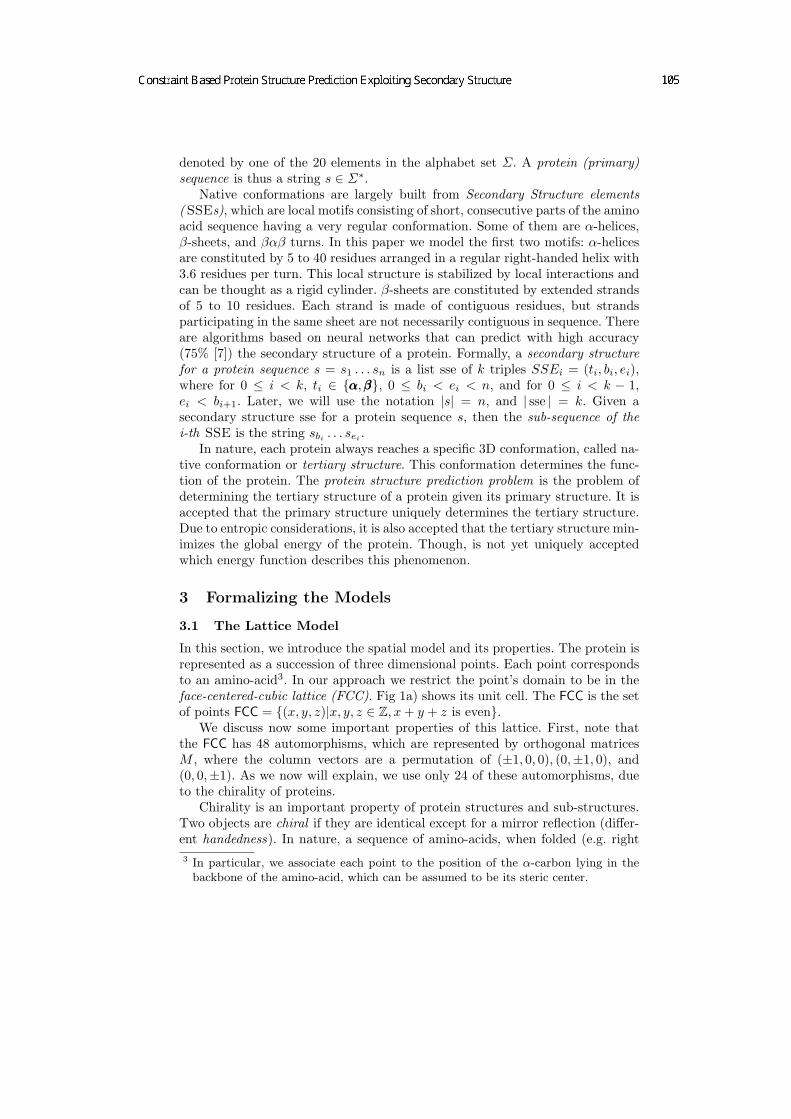
denoted by one of the 20 elements in the alphabet set Σ. A protein (primary)sequence is thus a string s ∈ Σ∗.

Native conformations are largely built from Secondary Structure elements(SSEs), which are local motifs consisting of short, consecutive parts of the aminoacid sequence having a very regular conformation. Some of them are α-helices,β-sheets, and βαβ turns. In this paper we model the first two motifs: α-helicesare constituted by 5 to 40 residues arranged in a regular right-handed helix with3.6 residues per turn. This local structure is stabilized by local interactions andcan be thought as a rigid cylinder. β-sheets are constituted by extended strandsof 5 to 10 residues. Each strand is made of contiguous residues, but strandsparticipating in the same sheet are not necessarily contiguous in sequence. Thereare algorithms based on neural networks that can predict with high accuracy(75% [7]) the secondary structure of a protein. Formally, a secondary structurefor a protein sequence s = s1 . . . sn is a list sse of k triples SSEi = (ti, bi, ei),where for 0 ≤ i < k, ti ∈ ααα,βββ, 0 ≤ bi < ei < n, and for 0 ≤ i < k − 1,ei < bi+1. Later, we will use the notation |s| = n, and | sse | = k. Given asecondary structure sse for a protein sequence s, then the sub-sequence of thei-th SSE is the string sbi . . . sei .

In nature, each protein always reaches a specific 3D conformation, called na-tive conformation or tertiary structure. This conformation determines the func-tion of the protein. The protein structure prediction problem is the problem ofdetermining the tertiary structure of a protein given its primary structure. It isaccepted that the primary structure uniquely determines the tertiary structure.Due to entropic considerations, it is also accepted that the tertiary structure min-imizes the global energy of the protein. Though, is not yet uniquely acceptedwhich energy function describes this phenomenon.

3 Formalizing the Models

3.1 The Lattice Model

In this section, we introduce the spatial model and its properties. The protein isrepresented as a succession of three dimensional points. Each point correspondsto an amino-acid3. In our approach we restrict the point’s domain to be in theface-centered-cubic lattice (FCC). Fig 1a) shows its unit cell. The FCC is the setof points FCC = (x, y, z)|x, y, z ∈ Z, x + y + z is even.

We discuss now some important properties of this lattice. First, note thatthe FCC has 48 automorphisms, which are represented by orthogonal matricesM , where the column vectors are a permutation of (±1, 0, 0), (0,±1, 0), and(0, 0,±1). As we now will explain, we use only 24 of these automorphisms, dueto the chirality of proteins.

Chirality is an important property of protein structures and sub-structures.Two objects are chiral if they are identical except for a mirror reflection (differ-ent handedness). In nature, a sequence of amino-acids, when folded (e.g. right3 In particular, we associate each point to the position of the α-carbon lying in the

backbone of the amino-acid, which can be assumed to be its steric center.

handed α-helices), has a specific handedness and usually it can not generate thesymmetric folding as well. In our model, when we apply transformations, weare interested in preserving the natural handedness. Since reflections invert thehandedness, we restrict to automorphisms with an orthogonal matrix with pos-itive determinant. Note that half of the possible automorphisms are reflections,since the determinant associated to the matrix is negative. This leads us to thefollowing definition of the basic transformation that we apply to points:

Definition 1. A matrix M is called rotational, if it is orthogonal, det(M) = 1and each of its elements is in Z. An isometric mapping 〈M, t〉, where t ∈ FCCand M is a rotational matrix, is a function from points to points of the form〈M, t〉 : p → Mp + t. We identify this function with its extension to sets ofpoints. M is called the transformation matrix of the isometric mapping 〈M, t〉and t its translation vector.

The composition A2 A1 of two isometric mappings A2 = 〈M2, t2〉 andA1 = 〈M1, t1〉, i.e. the application of A2 after A1 equals

〈M2, t2〉 〈M1, t1〉 = 〈M2M1,M2t1 + t2〉.

Note that A2 A1 is again an isometric mapping, since M2M1 is rotational.Due to this definition, there is also an inverse for an isometric mapping 〈M, t〉,namely 〈M, t〉−1 , 〈M−1,−M−1t〉. We define the FCC-norm of a point (x, y, z):

‖p‖fcc = max|x|, |y|, |z|, |x|+ |y|+ |z|

2

.

A vector v ∈ FCC is called a unit vector if ‖v‖fcc = 1. The FCC-distance of twopoints p, q ∈ FCC is ‖p−q‖fcc. Let us observe that in the FCC lattice, each walkfrom (0, 0, 0) to (x, y, z) ∈ FCC, needs at least ‖(x, y, z)‖fcc lattice unit vectors.We also use the standard Euclidean norm ‖〈x, y, z〉‖2 =

√x2 + y2 + z2.

3.2 The Protein Model

We provide here the formal definition of our 3D model and energy function. Thetertiary structure of a protein can be modeled as a function ω : [0 .. n−1] → FCC.The position of the i-th monomer in the protein corresponds to the point ω(i).

Definition 2. The function ω is a folding for the primary sequence s, iff

bond-constraint: ∀i . 0 ≤ i < |s| − 1 : ‖ω(i)− ω(i + 1)‖fcc = 1, andangle-constraint: ∀i . 0 ≤ i < |s|−2 : ∠(ω(i), ω(i+1), ω(i+2)) ∈ 90, 120, 180.

Note that we allow only angles of 90, 120, and 180, whereas in the FCClattice, three consecutive monomers can also form angles of 0 and 60. Weexclude the angles less than 90 for sterical reasons, since the first and thirdamino-acid would be too close. Note that in [10] the 180 angle was excludedas well, since it is unfavorable in real proteins. In our approach we allow thisangle, since simpler constraints can be used (especially when linking SSEs to

neighbors). Moreover, when discretizing the protein on FCC lattice, 180 anglescan be required to fit more accurately the native state. For example, the modelingof α-helices in the FCC lattice, is not able to represent the typical periodicity ofthe pattern.

A folding ω satisfies a secondary structure sse = (ti, bi, ei)0≤i<| sse | if andonly if for every i ∈ [0..| sse | − 1], the positions ω(bi), . . . , ω(ei) approximate aright-handed α-helix on the FCC if ti = ααα and approximate a β-strand on the FCCif ti = βββ. We give a formal definition of these approximations in Subsection 5.1.

The modeling of the folding energy is a delicate issue: a large set of phe-nomena can be included to produce a refined energy function. In this paper werestrict to one kind of interaction between elements, namely the contact energybetween pairs of amino-acids and we use the matrix developed in [6]. ppot(a, b)denotes the potential of the amino-acids a and b. The potential is only con-tributed to the total energy if the two amino-acids are in close contact. If twomonomers are too close, they are clashing, in this case the total energy is ∞,since for steric reasons two residues repel each other.

Definition 3 (Energy). For two amino-acids a, b ∈ Σ and two positions p, q ∈FCC, we define

E(a, b, p, q) =

ppot(a, b) ‖q − p‖2 = 2∞ ‖q − p‖2 < 20 otherwise.

The energy of a protein conformation with protein sequence s and foldingω : [0 .. |s| − 1] → FCC is EC(s, ω) =

∑0≤i,j<|s|,i+2<j E(si, sj , ω(i), ω(j)).

Note that due to our definition, every sub-sequence up to 3 consecutiveamino-acids in the primary structure, does not contribute to the energy. Thisis an empirical choice. Basically, if three consecutive amino-acids formed an an-gle of 90 the first and third amino-acid would form a pair contributing to theenergy, whereas if they formed an angle of 120 there would be no contribu-tion. The energy contribution of an amino-acid pair is negative on average andthus, angles of 90 would be always favoured. This is true in the lattice, butnot in nature, and thus we avoid this a-priori preference by removing the energycontribution of the pair of amino-acids si and si+2.

We report here a part of the potential table of [6], also available at http://www.dimi.uniud.it/dovier/PF/.

CYS MET PHE ILE LEU VAL TRP TYR ALA GLY

CYS -3.477 -2.240 -2.424 -2.410 -2.343 -2.258 -2.080 -1.892 -1.700 -1.101MET -2.240 -1.901 -2.304 -2.286 -2.208 -2.079 -2.090 -1.834 -1.517 -0.897PHE -2.424 -2.304 -2.467 -2.530 -2.491 -2.391 -2.286 -1.963 -1.750 -1.034· · · · · ·

4 Problem Definition and Solving Strategy

We define the protein structure prediction problem when the secondary structureinformation is taken into account. Given a sequence s and a secondary structure

sse, the problem is to find the folding ω that satisfies sse and has minimal energyEC(s, ω). The energy function can be partitioned as a sum of four energy terms,namely the energy contribution by pairs of amino-acids, where

1. both are in the same SSE,2. both are in SSEs, but not in the same,3. one is in a SSE and the other is not,4. both are not in SSEs.

Formally, these contributions, whose sum is EC(s, ω) are defined as

1. Es(s, sse, ω) =∑

0≤r<| sse |∑

br≤i+2<j≤erE(si, sj , ω(i), ω(j))

2. Ess(s, sse, ω) =∑

0≤r<r′<| sse |∑

br≤i≤er

∑b′r≤j≤e′r,i+2<j E(si, sj , ω(i), ω(j))

3. Esn(s, sse, ω) =∑

i∈D

∑0≤j<|s|,j 6∈D,i+2<j E(si, sj , ω(i), ω(j))

4. Enn(s, sse, ω) =∑

0≤i<j<|s|,i,j 6∈D,i+2<j E(si, sj , ω(i), ω(j)),

where D is the set of positions in SSE, i.e.⋃

0≤r<| sse |[br .. er]. The first termEs(s, sse, ω) is constant for each folding ω that satisfies a given secondary struc-ture sse. Thus, optimizing EC(s, ω) it is equivalent to optimize Ess(s, sse, ω) +Esn(s, sse, ω) + Enn(s, sse, ω).

From a set of 500 selected PDB-proteins, we estimated the average contribu-tions of the last three terms to their sum in the native state, which is given by thefollowing distributions: Ess 49% , Esn 36%, and Enn 15%. Note that half of theenergy is contributed by interaction between SSEs. This suggests a heuristic tosolve the structure prediction problem. Thus, first we place the SSEs optimallyaccording to Ess. Then, for fixed SSEs, we place the remaining amino-acids whileoptimizing EC(s, ω).

During the optimization of Ess, the SSEs are placed in the FCC lattice. Theelements are treated as rigid blocks that can be shifted and oriented in thelattice. It is fundamental to be independent from global rigid transformations,which give the same isomorphic results. In the next section, we introduce thenotion of relative position between two SSEs. This concept is the base to ab-stract from the symmetries of the problem. Note that all energy terms are basedon the notion of distance between amino-acids, thus they are invariant underrigid transformations. The relative position description, thus, is suitable to beassociated to a specific energy contribution provided by the represented class.

5 Absolute and Relative Positions

In this section, we discuss a formalism to describe the SSEs and their placementin the lattice. We specify an object (later denoted by template) by a list of FCCpoints. The object is placed in the space by transforming these points by meansof rotating and translating. This transformation defines the absolute positionof the placed object (later denoted by instance). We also introduce the relativeposition of two SSEs, which is the transformation required to map the absoluteposition of the first element into the one of the second. Fig. 1b) provides anillustration of the concepts that are introduced in this section.

(a)

2

3

4

1

A

C

B

(b)

Fig. 1. a) Unit Cell of the face-centered cubic lattice (FCC). There is one point in eachcorner of a cube and one point in the center of each face. We show the connections byunit vectors. b) Idea of absolute and relative positions. The figure shows instances ahelix template of length 8 and type 0 and a sheet template of length 6. If the instances 1and 2 are in absolute position id, then A (resp. B) is the absolute position of the instance3 (resp. 4). C = ρ(A, B) is the relative position between the instances (from A to B).We show local coordinate systems for each instance to illustrate the transformation.

5.1 Templates

A template is a function T : [0 .. ` − 1] → FCC, where ` ∈ N is its length. Weintroduce two classes of templates, namely α-helices and β-sheets. In these cases,a template is the geometric description of a helix (sheet) starting from (0, 0, 0).

Definition 4 (Templates for SSEs). Let a function h : N→ FCC be given byh(4i+0) = (0, 0, 0)+ i dh, h(4i+1) = (1, 0, 1)+ i dh, h(4i+2) = (2, 0, 0)+ i dh,and h(4i + 3) = (2, 1,−1) + i dh for i ∈ N, where dh = (2, 2, 0). Then, the helixtemplate of length n and type τ , where n ∈ N and τ ∈ 0, 1, is the functionhelixτ

n : [0 .. n− 1] → FCC, helixτn(i) = h(i− τ) (i ∈ [0 .. n− 1]).

Furthermore, let a function sheetn : [0 .. n−1] → FCC, be given by s(2i+0) =(0, 0, 0) + i ds and s(2i + 1) = (1, 1, 0) + i ds for i ∈ N, where ds = (2, 0, 0).

Note that the helix templates of type 0 (resp. 1) describe helices, where thefirst three points form an angle of 90 (resp. 120).

5.2 Position of an Instance

Definition 5 (Absolute Position, Instance). An absolute position is anisometric mapping. An instance I with absolute position 〈M, t〉 of a template Tis a pair I = 〈M, t〉♦T. The instance function of I, denoted by I fun, is 〈M, t〉T .

For i ∈ Z, we use the short notations I(i) for I fun(i) and dom(I) for dom(I fun).The image of an instance I is img(I) = I(i)|i ∈ dom(I).

The instance function of the instance 〈id, (0, 0, 0)〉♦T is 〈id, (0, 0, 0)〉T = T .

Definition 6 (Relative Position). For instances Ii with absolute positions Ai

(i = 1, 2), the relative position ρ(A1, A2) from A1 to A2 is the isometric mapping,where ρ(A1, A2) = A−1

1 A2. Then, ρ(A1, A2) is also called the relative positionof the instances I1 and I2.

The relative position between two instances Ii = Ai♦Ti (i = 1, 2) can be usedto obtain the second instance from the first instance as I2 = A1 ρ(A1, A2)♦T2,since by definition A2 = A1 ρ(A1, A2).

The following proposition claims that the relative position of two instancesis invariant under global transformations.

Proposition 1. Given the instances Ii = Ai♦Ti, I′i = A′i♦T ′i (i=1,2), the rel-

ative positions R = ρ(A1, A2), R′ = ρ(A′1, A′2) and the isometric mappings Ci,

such that A′i = Ci Ai, then R = R′ if and only if C1 = C2.

Note that by Proposition 1, ρ(M A1,M A2) = ρ(A1, A2) for isometricmappings M , A1, and A2. Especially, for every relative position ρ(A1, A2), thereis an identical relative position of the form ρ(id, B) = B for some isometricmapping B, namely B = A−1

1 A2.

6 Energy contribution of instance pairs

In the first phase of the algorithm, we pre-compute the energy contributionof a pair of instances in every relevant placement. Therefore, we enumeratethe set of relative positions between the instances of two templates, where thetwo instances interact sterically. Only for those relative positions, the energycontribution is not equal to zero.

Definition 7 (Interaction). Two instances I1 and I2 interact, if and only ifthere exist i1 ∈ dom(I1), i2 ∈ dom(I2), such that ‖I2(i2) − I1(i1)‖2 ≤ 2. Wedefine the interaction set of templates T1 and T2 as InteractionSet(T1, T2) =

R = ρ(id, R) | I1 = id ♦T1, I2 = R♦T2, I1 and I2 interact.Note that in the definition, we have in mind to fix the first instance (here

to id) and move the second instance to every interacting position. Nevertheless,due to Proposition 1, the interaction set contains all relative positions betweenarbitrary instances that are interacting. Note that the interaction set is finite,since the instances are finite.

If we define neighVecs as a tuple of the 19 vectors p ∈ FCC with ‖p‖2 ≤ 2in arbitrarily fixed order, then for a template T , we define an extended templateT ext by T ext(19 · i + j) = T (i) + neighVecsj , for i ∈ dom(T ) and 0 ≤ j < 19.

We say that two instances intersect if and only if their images have a non-empty intersection.

Proposition 2. Two instances I1 = A1♦T1 and I2 = A2♦T2 interact if andonly if Iext

1 = A1♦T ext1 and I2 intersect.

Definition 8 (Energy Contribution). Two instances of templates Ti withsequence si (i = 1, 2) with relative position R give an energy contribution of

ET(s1, s2, T1, T2, R) =∑

0≤j<|s1|,0≤k<|s2|E(s1j , s2k, id ♦T1(j + b1), R♦T2(k + b2)), (1)

where b1 = min(dom(T1)) and b2 = min(dom(T2)).

Recall that for the templates T1 and T2, there are only finitely many relativepositions R, such that id ♦T1 and R♦T2 interact, i.e. InteractionSet(T1, T2) isfinite. By merging the two definitions of interaction and the energy contributionof a pair of amino-acids, if ET(s1, s2, T1, T2, R) is different from 0, then id ♦T1 andR♦T2 interact. Note that from the interaction of id ♦T1 and R♦T2, we can notconclude that ET(s1, s2, T1, T2, R) 6= 0, since depending on the table of pairwisepotentials certain interaction patterns of the two instances could sum up to 0.

Due to this, in order to completely give the energy for every relative posi-tion R it suffices to consider all R ∈ InteractionSet(T1, T2). Now, the problemdiscussed in this subsection reduces to generate InteractionSet(T1, T2). Insteadof enumerating the relative positions, where instances of T1 and T2 interact, weequivalently enumerate the relative positions, where instances of T ext

1 and T2

intersect. Due to the following proposition, we can completely enumerate the setInteractionSet(T1, T2).

Proposition 3. For templates T1 and T2,

InteractionSet(T1, T2) =⊎

M rot. matrix

〈M, t〉|∃j1, j2 : id ♦T ext1 (j1) = 〈M, t〉♦T2(j2).

Proof. Obviously, one can partition any interaction set by the rotation matricesof the relative positions. Then, the proposition is a consequence of Proposition 2.

For the inclusion ⊆, let R = 〈M, t〉 in InteractionSet(T1, T2). Then, the in-stances id ♦T1 and R♦T2 interact, i.e. the instances id ♦T ext

1 and R♦T2 intersect.For the inclusion ⊇, for any R = 〈M, t〉 in one of the subsets 〈M, t〉|∃j1, j2 :

id ♦T ext1 (j1) = 〈M, t〉♦T2(j2), the instances id♦T ext

1 and R♦T2 intersect. Thus,id ♦T1 and R♦T2 interact. ¤

The proposition suggests the following algorithm. For every rotation matrixM , for every pair of indices j1 ∈ dom(T1) and j2 ∈ dom(T2), collect the uniquetranslation vectors t, where id ♦T ext

1 (j1) = 〈M, t〉♦T2(j2).Note that there is indeed a unique t for every M , j1 and j2, which is calculated

in constant time. Also note that whereas this algorithm can enumerate a vectort more than once, the algorithm still calculates only a limited number of 24 ×| img(T ext

1 )| × | img(T2)| many vectors t.

7 Constraint Model

Recall, that we discuss the problem of finding the folding ω for a given proteinsequence s and a given secondary structure sse = (ti, bi, ei)0≤i<| sse |, that satisfiessse and has minimal energy EC(s, ω). We already suggested a heuristic for theminimization, which consists of two separate phases and uses the outcome of thealready described computation of energy contributions of instances.

In a first branch-and-bound search, we place the secondary-structure ele-ments (SSEs) while optimizing the energy contribution Ess, i.e. we search fora folding ω that satisfies sse and has minimal energy Ess(s, sse, ω) and a finite

total energy EC(s, ω). For finite energy EC(s, ω), there must not be clashes inthe tertiary-structure. When we place only the SSEs, we can not check the non-clashing of the remaining amino-acids efficiently by consistency methods. Hence,we search for one consistent placing of the remaining amino-acids each time wefind a new placement of the SSEs. Then, a second branch-and-bound searchcomputes a placement of SSEs and remaining amino-acids that optimizes thetotal energy EC(s, ω) and places the SSEs nearly optimally w.r.t. Ess.

All the constraints and the enumeration strategy are common for the twophases. Due to this, we are able to give only a common description as well as toimplement only a single solver in our implementation language Oz 3.0 [15].

The constraint model as well as our enumeration strategy divides into twoparts. The first part deals with the placement of the SSEs, whereas the secondpart handles the placement of the remaining amino-acids. The focus of our workis on the first part and only this part shall be described in more detail.

In the first part, we use the pre-computed energy contributions of instancepairs. Therefore, we start with relating our placement problem to the notion oftemplates and instances.

We define templates for every SSE in sse. For each SSE k, we introducean absolute position Ak and a type τk ∈ 0, 1, 2, where 0 ≤ k < | sse |. Sucha type τk combines the distinction between α-helix and β-sheet with the typesof helix-templates (cf. Def 4). For a helix, this type gives just the type 0 or 1of the corresponding helix-template and for sheets this type is always 2. For0 ≤ k < | sse |, where tk = ααα, we define T τ

k = helixτek−bk+1 (τ = 0, 1) and where

tk = βββ, we define T 2k = sheetek−bk+1. Let sk denote the sub-sequence of the

k-th SSE. We define Iτk as Ak♦T τ

k for absolute positions Ak. Now, the tertiary-structure ω is related to the instances, by ω(i) = Ak♦T τk

k (i−bk) for i ∈ [bk .. ek].Then, for given template definitions, the positions of amino-acids in SSEs

are completely specified by (Ak)0≤k<| sse | and (τk)0≤k<| sse |. Due to this, we canequivalently investigate the problem in terms of instances. The relation betweenthe instances determines the energy term Ess. In the same time the relations areconstrained by the properties of a folding.

We choose to enumerate the relative positions of the elements instead theirabsolute positions.4 Besides breaking of symmetries5, there are several advan-tages in enumerating relative positions instead absolute positions. Most notably,there is a direct correspondence between the relative position and the energycontribution of a pair of SSEs. This immediate relation is used to dynamicallyguide the search, i.e. we enumerate highly contributing relations between SSEsfirst. Furthermore, enumerating relative positions is more general than enumer-ating absolute positions. Imagine, that we enumerate absolute positions. Then,after w.l.o.g. fixing the absolute position of the first instance to 〈id,0〉, enumerat-ing the absolute positions of the remaining elements is equivalent to enumerating

4 Notably, the energy contribution Ess is determined only from the relative positions.5 Note that by using relative positions instead absolute positions, we break all geo-

metrical symmetries in the problem for free. In general, breaking of symmetries inconstraint modeling is a non-trivial task and a broadly discussed topic (e.g. see [2]).

their relative positions to the first element. In contrast, our more flexible enu-meration strategy can dynamically decide to enumerate relations earlier thatcontribute stronger to the total energy than any relation to the first element.

As described in the previous section, we are able to calculate the energy con-tribution of two instances in every relative position and in particular enumeratethe finite list of relative positions, where this energy contribution differs fromzero. For every pair of SSEs in sse, we generate such a list of relative positionsand corresponding energy contributions. Since for α-helices there are two typesof helix-templates, we also include the information on the type in the list foreach pair of SSEs. Here, it is convenient to partition the list into two tables:NTabij and CTabij . In the former table, we include every relative position thatproduces a finite, non-zero energy (i.e. there is an interaction but no clash for thisrelative position), and in the latter we collect all relative positions, where the ele-ments i and j clash (infinite energy). In preparation of our enumeration strategy,the tables NTabij are ordered by increasing energy-values. For being uniform,we generate for every pair of secondary-structure elements i and j, the tablesNTabij and CTabij , which consist of all records (σi, σj , R, E), where σi (resp.σj) is a possible value for the type τi (resp. τj) and R ∈ InteractionSet(T σi

i , Tσj

j ).Then, E is the corresponding energy contribution ET(si, sj , T

σii , T

σj

j , R). 6

7.1 Variables and Constraints

First, for 0 ≤ i < j < | sse | we introduce finite-domain variables Xij , where thedomain of the variable Xij is [0 .. |NTabij | − 1] ] ∆. The value of Xij is eitheran index in the table NTabij or ∆. In the first case, the relation (i.e. relativeposition Rij and helix-types) between the SSEs i and j is specified by the Xij-thentry in the table NTabij . The case Xij = ∆ represents those relative positionsthat provide no energy contribution, but cause a distance of elements i and jthat still allows to connect the elements in a folding.

Since the variables Xij completely specify the relative positions only forXij 6= ∆, we introduce an explicit representation of relative positions for en-suring consistency. The relative position between the elements i and j is givenby variables RM

ij , which encodes for the transformation matrix of Rij , and Rxij ,

Ryij , and Rz

ij , which represent the coordinates of the translation vector of Rij .The domain of RM

ij is finite, since there are only 24 rotational matrices. Alsothe variables Rx

ij , Ryij , and Rz

ij have finite-domains, since the number of transla-tions is limited due to the bond-constraint connecting the amino-acids betweenelements i and j. Since the tuple (RM

ij , Rxij , R

yij , R

zij) represents one relative po-

sition, we address this tuple as the variable Rij . For 0 ≤ i < | sse |, we addvariables Typei ∈ 0, 1, 2, which correspond to the types τi of the SSEs. Ifti = ααα, the value of Typei gives the type of the helix 0 or 1. For ti = βββ, we setTypei = 2. The variables Rij , Typei and Typej are related to the variable Xij via

6 Note that in these tables we represent the rotational matrices of the relative positionsby unique indices in the interval [0 .. 23]. This representation is also used to modeldomains of matrices with integer finite domain variables.

the table NTabij . This relation is handled by a native propagator7, which doesonly cheap propagation, if sufficiently many variables are ground. Furthermore,it checks the validity of the encoded isometric mapping (w.r.t. clashes and thebond-constraint). Also the relation between the relative position variables Rij

that corresponds to the transitivity Rij Rjk = Rik is only propagated in suchsimple cases.

Finally, the energy contribution Ess is computed in a variable Energyss as thesum of variables Energyij . These variables denote the energy that is contributedby the elements i and j in the relation that is specified by Xij .

The essential propagation in our approach is done by a propagator for thetransitivity constraint Rij Rjk = Rik on the variables Xij . This propagator hasto relate the indices in the domains of the variables Xij to the correspondingrelations. Moreover, it has to handle ∆-values in the domains correctly. For thisreason, this propagator distinguishes several cases. Case 1) At least two of thevariables are determined to ∆. In this case no further propagation can be applied.Case 2) The domains of all three variables contain ∆. Then, at this stage wecan not derive any information. Case 3) The domains of exactly two variablescontain ∆. Here, the domain without ∆ is used to prune the other two domains.W.l.o.g. let us assume that Xjk and Xik contain ∆. We now describe how toprune the domain of Xjk. For every isometric mapping B indexed by Xjk wecheck if there exists at least one isometric mapping A indexed by Xij such thatA B is indexed by a value of Xik. If there is no support, the index is removedfrom the domain of Xjk. The analogous procedure is applied to prune Xik. Case4) The domain of at most one variable contains ∆. W.l.o.g. assume that Xik

contains ∆. Then, we collect the composition of every pair from the domains ofXij and Xjk and intersect the result with the domain of Xik. Moreover, we prunethe domains of Xij and Xjk using the technique of the previous item. Note thatduring this propagation, we compose only isometric mappings from the tableswith consistent types in the same table rows.

To give some implementation details, note that in Oz, every index variablehas a range that begins from 1. Moreover, since Oz does not support nega-tive values in finite domains, we shift the domains of variables Rx

ij , Ryij , R

zij and

in all energy variables accordingly. For convenience, we represent the ∆ valuedifferently for each i, j with the integer value |NTabij |. Due to the complexpropagation of the transitivity constraint for the variables Xij , we preferred toimplement the propagator in C++, recalling it inside the Mozart code.

7.2 Search Strategy

For placing the SSEs, we enumerate the variables Xij in a dynamic enumerationorder, which combines a first-fail strategy with a preference for variables Xij thatallow a strong contribution to the energy Ess. Here, we find the best contributionthat is allowed by the variable Xij , if we look up in the table NTabij using thelowest possible value of Xij as index. Recall that the tables NTabij are ordered7 In Oz, a native propagator is a propagator implemented in C++. For the purpose

of writing special propagators, Oz is extensible via its C++-interface [11].

by increasing energy, in particular for this purpose. As value we will always selectthe minimal value in the domain, which again corresponds to the optimal energycontribution of the elements i and j.

We will only enumerate the variables Xij in order to find a good placement ofSSEs. Note that since we can assign ∆ to variables Xij , not every assignment ofthese variables completely determines a placement. However, we will only con-sider placements that are completely determined after the enumeration of thevariables Xij . This is justified as a heuristic, since we only search for energeti-cally good placements and such placements will have many strong interactionsbetween the elements. In this situation, there are usually many variables Xij 6= ∆,which then determine the remaining relative positions.

In practice, we apply also a filtering of the domains of the variables Xij bytheir energy. Since the special element ∆ also represents the filtered elements,the constraint problem is not changed, except that the energy is calculated lessaccurately. Filtering these domains has two conflicting impacts. Whereas strongfiltering on the domain sizes results in faster enumeration, larger domains achievea stronger propagation (due to the transitivity constraints). For that reason, weapply two filters. First, we filter the tables NTab to contain only entries withenergies in a range of x% of the optimal energy. The filtered tables constitute thedomains of the variables Xij. The second filtering affects only the enumeration,where we enumerate only values within a range of y% (y < x) of the optimum.With careful filtering we are able to reduce search times, while preserving agood quality of the results. The strategy is justified, since good placements haveusually sufficiently many high scoring pairwise energy contributions.

After the SSEs are placed, we compute absolute positions of their amino-acids by fixing the absolute position of the first element (thereby breaking thesymmetries). Then, the positions of the remaining amino-acids are enumeratedusing a first-fail strategy combined with a preference for good energy contribu-tion. Constraints ensure non-clashing and calculate the remaining energy termEnn +Esn in a variable Energynss.

8 Results

We implemented the described constraint-model in the programming languageOz 3.0 [15] using its most recent implementation Mozart 1.3.0. We extended thelanguage by special constraint propagators written in C++. Also the computa-tion of the energy contributions of instance-pairs is implemented in C++. Theimplementations are available via http://www.bio.inf.uni-jena.de.

For evaluating our result, we ran the prediction for proteins with knownstructure from the PDB [5]. All predictions are performed on a Pentium 4 at2.4GHz. Figure 2 shows our prediction for the protein domain “Maternal effectprotein Staufen” with PDB-code 1STU in comparison to the known tertiarystructure. The protein consists of 68 residues, forming two α-helices and threeβ-sheets. The computation of the energy contribution of instances was performedin 14 seconds. In the first search, we found a good placement of the SSEs in 3.5

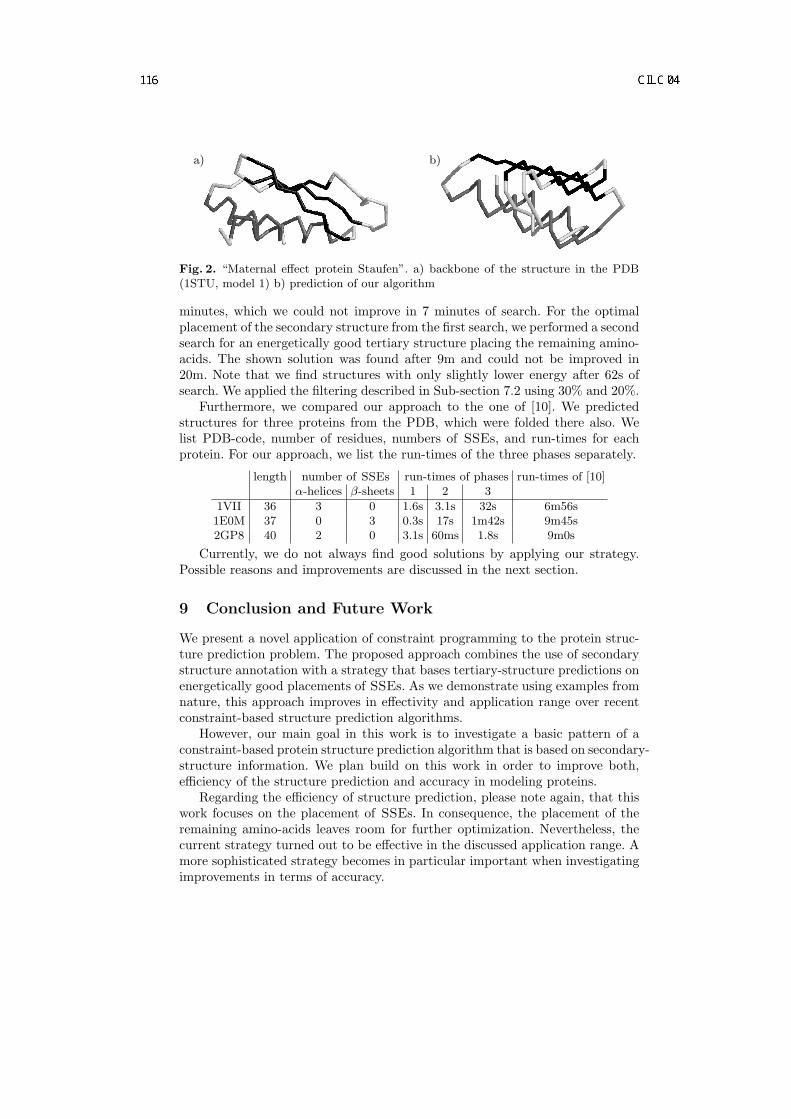
a) b)

Fig. 2. “Maternal effect protein Staufen”. a) backbone of the structure in the PDB(1STU, model 1) b) prediction of our algorithm

minutes, which we could not improve in 7 minutes of search. For the optimalplacement of the secondary structure from the first search, we performed a secondsearch for an energetically good tertiary structure placing the remaining amino-acids. The shown solution was found after 9m and could not be improved in20m. Note that we find structures with only slightly lower energy after 62s ofsearch. We applied the filtering described in Sub-section 7.2 using 30% and 20%.

Furthermore, we compared our approach to the one of [10]. We predictedstructures for three proteins from the PDB, which were folded there also. Welist PDB-code, number of residues, numbers of SSEs, and run-times for eachprotein. For our approach, we list the run-times of the three phases separately.

length number of SSEs run-times of phases run-times of [10]α-helices β-sheets 1 2 3

1VII 36 3 0 1.6s 3.1s 32s 6m56s1E0M 37 0 3 0.3s 17s 1m42s 9m45s2GP8 40 2 0 3.1s 60ms 1.8s 9m0s

Currently, we do not always find good solutions by applying our strategy.Possible reasons and improvements are discussed in the next section.

9 Conclusion and Future Work

We present a novel application of constraint programming to the protein struc-ture prediction problem. The proposed approach combines the use of secondarystructure annotation with a strategy that bases tertiary-structure predictions onenergetically good placements of SSEs. As we demonstrate using examples fromnature, this approach improves in effectivity and application range over recentconstraint-based structure prediction algorithms.

However, our main goal in this work is to investigate a basic pattern of aconstraint-based protein structure prediction algorithm that is based on secondary-structure information. We plan build on this work in order to improve both,efficiency of the structure prediction and accuracy in modeling proteins.

Regarding the efficiency of structure prediction, please note again, that thiswork focuses on the placement of SSEs. In consequence, the placement of theremaining amino-acids leaves room for further optimization. Nevertheless, thecurrent strategy turned out to be effective in the discussed application range. Amore sophisticated strategy becomes in particular important when investigatingimprovements in terms of accuracy.

For the aspect of accuracy, we consider it promising to investigate in par-ticular four improvements: refinement of solutions by stochastic optimization,using more complex energy functions (e.g., Lennard-Jones potential), modelingthe tertiary-structure off-lattice, and modeling sidechains of amino-acids.

Acknowledgments

The authors thank Federico Fogolari for several useful discussions. A. Dal Paluand A. Dovier are partially supported by MIUR Project Verifica di sistemi reat-tivi basata su vincoli (COVER) and by FSE project Misura D4.

References

1. R. Backofen. The protein structure prediction problem: A constraint optimizationapproach using a new lower bound. Constraints, 6(2–3):223–255, 2001.

2. R. Backofen and S. Will. Excluding symmetries in constraint-based search. Con-straints, 7(3):333–349, 2002.

3. Z. Bagci, R. L. Jernigan, and I. Bahar. Residue coordination in proteins conformsto the closest packing of spheres. Polymer, 43:451–459, 2002.

4. Z. Bagci, R. L. Jernigan, and I. Bahar. Residue packing in proteins: Uniformdistribution on a coarse-grained scale. J Chem Phys, 116:2269–2276, 2002.

5. H. M. Berman, J. Westbrook, Z. Feng, G. Gilliland, T. N. Bhat, H. Weissig, I. N.Shindyalov, and P. E. Bourne. The protein data bank. Nucleic Acids Research,28:235–242, 2000. http://www.rcsb.org/pdb/.

6. M. Berrera, H. Molinari, and F. Fogolari. Amino acid empirical contact energydefinitions for fold recognition in the space of contact maps. BMC Bioinformatics,4(8), 2003.

7. R. Bonneau and D. Baker. Ab initio protein structure prediction: progress andprospects. Annu. Rev. Biophys. Biomol. Struct., 30:173–89, 2001.

8. B. Cipra. Packing challenge mastered at last. Science, 281:1267, 1998.9. P. Crescenzi, D. Goldman, C. Papadimitrou, A. Piccolboni, and M. Yannakakis.

On the complexity of protein folding. In Proc. of STOC, pages 597–603, 1998.10. A. Dal Palu, A. Dovier, and F. Fogolari. Protein folding in CLP (FD) with empir-

ical contact energies. In Recent Advances in Constraints, volume 3010 of LectureNotes in Computer Science, pages 250–265. Springer-Verlag, Berlin, 2004.

11. T. Muller and J. Wurtz. Interfacing propagators with a concurrent constraintlanguage. In JICSLP96 Post-conference workshop and Compulog Net Meeting onParallelism and Implementation Technology for (Constraint) Logic ProgrammingLanguages, pages 195–206, 1996.

12. B. H. Park and M. Levitt. The complexity and accuracy of discrete state modelsof protein structure. Journal of Molecular Biology, 249(2):493–507, 1995.

13. B. Rost and C. Sander. Prediction of protein secondary structure at better than70% accuracy. Journal of Molecular Biology, 232(2):584–99, 1993.

14. J. Skolnick and A. Kolinski. Computational studies of protein folding. Computingin Science and Engineering, 3(5):40–50, 2001.

15. G. Smolka. The Oz programming model. In Computer Science Today: RecentTrends and Developments. Springer-Verlag, Berlin, 1995.

16. S. Will. Constraint-based hydrophobic core construction for protein structure pre-diction in the face-centered-cubic lattice. In Proceedings of the Pacific Symposiumon Biocomputing 2002 (PSB 2002).

Using a theorem prover for reasoning on

constraint problems

Marco Cadoli and Toni Mancini

Dipartimento di Informatica e SistemisticaUniversita di Roma “La Sapienza”

Via Salaria 113, I-00198 Roma, Italycadoli|tmancini@dis.uniroma1.it

Abstract. Specifications of constraint problems can be considered logi-cal formulae. As a consequence, it is possible to infer their properties bymeans of automated reasoning tools. The purpose of this paper is exactlyto link two important technologies: automated theorem proving and con-straint programming. We report the results on using a theorem proverand a finite model finder for checking existence of symmetries, checkingwhether a given formula breaks a symmetry, and checking existence offunctional dependencies among groups of predicates. As a side-effect, wepropose a new domain of application and a brand new set of benchmarksfor ATP systems.

1 Introduction

The style used for the specification of a combinatorial problem varies a lot amongdifferent languages for constraint programming. In this paper, rather than con-sidering procedural encodings such as those obtained using libraries (in, e.g.,C++ or prolog), we focus on highly declarative languages. In fact, manysystems and languages for the solution of constraint problems (e.g., ampl [9],opl [20], gams [5], dlv [7], smodels [18], and np-spec [4]) clearly separatethe specification of a problem, e.g., graph 3-coloring, and its instance, e.g., agraph, using a two-level architecture for finding solutions: the specification is in-stantiated (or grounded) against the instance, and then an appropriate solver isinvoked. There are several benefits in this separation: obviously declarativenessincreases, and the solver is completely decoupled from the specification. Ideally,the programmer can focus only on the specification of the problem, without com-mitting a priori to a specific solver. In fact, some systems, e.g., ampl [9], areable to translate –at the request of the user– a specification in various formats,suitable for different solvers.

Again, the syntax varies a lot among such languages: ampl, opl, and gams

allow the representation of constraints by using algebraic expressions, while dlv,smodels, and np-spec are rule-based languages. Anyway, from an abstractpoint of view, all such languages are extensions of existential second-order logic(ESO) on finite databases, where the existential second-order quantifiers andthe first-order formula represent, respectively, the guess and check phases of the

specSolver

(Instantiation& Solving)

outputtransf’d

spec

instance

searchstrategy

(Transformation)Prover

TheoremAutomated

Fig. 1. Architecture of the problem solving system.

constraint modelling paradigm. In particular, in all such languages it is possibleto embed ESO queries, and the other way around is also possible, as long as onlyfinite domains are considered.

Since specifications are logical formulae, it is possible to infer their propertiesby means of automated reasoning tools. The purpose of this paper is exactly tolink two important technologies: automated theorem proving (ATP) and con-straint programming. The architecture of the system we envision is representedin Figure 1.

In particular, we report the results on using a theorem prover and a finitemodel finder for reasoning on specifications of constraint problems, representedas ESO formulae. We focus on two forms of reasoning:

– checking existence of value symmetries, i.e., properties of the specificationthat allow to exchange values of the finite domains without losing all solu-tions; on top of that, we check whether a given formula breaks such symme-tries;

– checking existence of functional dependencies, i.e., properties that force val-ues of some guessed predicates to depend on the value of some others.

There are at least two reasons why a system should make automatically suchchecks: first of all, it has been proven that solving can be made much more effi-cient by, e.g., recognizing and breaking symmetries (a wide literature is nowadaysavailable, cf., e.g., [2, 6]). Secondly, the person performing constraint modellingmay be interested in the above properties: as an example, existence (or lack) ofa dependency may reveal a bug in the specification.

The main result of this paper is that it is actually possible to use ATP tech-nology to reason on combinatorial problems, and we exhibit several examplesproving it. As a side-effect, we propose a new domain of application and a brandnew set of benchmarks for ATP systems, which is not represented in large repos-itories, such as TPTP (cf. www.tptp.org).

Relations between constraint satisfaction and deduction have been observedsince several years (cf., e.g., the early work [1], and [12] for an up-to-date report).The use of automated tools for preprocessing constraint satisfaction problems(CSPs) has been limited, to the best of our knowledge, to the instance level.As an example, the use of packages such as nauty [16] for finding symmetries

on CSPs has been proposed in [6]. On the other hand, not much work hasbeen done on reasoning at the specification level. A limited form of reasoning isoffered by the opl system, which checks (syntactically) whether a specificationcontains only linear constraints and objective function, and in this case invokesan integer linear programming solver (typically very efficient); otherwise, it usesa constraint programming solver.

The rest of the paper is organized as follows: in Section 2 we give some pre-liminaries on modelling combinatorial problems as formulae in ESO. Sections 3and 4 are devoted to the description of experiments in checking symmetriesand dependencies, respectively. In Section 5 we conclude the paper, and presentcurrent research.

2 Preliminaries

In this paper, we use existential second-order logic (ESO) for the specificationof problems, which allows to represent all search problems in the complexityclass NP [8]. The use of ESO as a modelling language for problem specificationsis common in the database literature, but unusual in constraint programming,therefore few comments are in order. Constraint modelling systems like thosementioned in Section 1 have a richer syntax and more complex constructs, andwe plan to eventually move from ESO to such languages. For the moment, weclaim that studying the simplified scenario is a mandatory starting point formore complex investigations, and that our results can serve as a basis for re-formulating specifications written in higher-level languages. Anyway, examplesusing the syntax of the implemented language opl are exhibited in Sections 4and 5.

Coherently with all state-of-the-art systems, we represent an instance of aproblem by means of a relational database. All constants appearing in a databaseare uninterpreted, i.e., they don’t have a specific meaning.

An ESO specification describing a search problem π is a formula ψπ

∃S φ(S,R), (1)

where R = R1, . . . , Rk is the relational schema for every input instance (i.e., afixed set of relations of given arities denoting the schema for all input instancesfor π), and φ is a quantified first-order formula on the relational vocabularyS ∪ R ∪ = (“=” is always interpreted as identity).

An instance I of the problem is given as a relational database over the schemaR, i.e., as an extension for all relations in R. Predicates (of given arities) in theset S = S1, . . . , Sn are called guessed, and their possible extensions (withtuples on the domain given by constants occurring in I plus those occurring inφ, i.e., the so called Herbrand universe) encode points in the search space forproblem π.

Formula ψπ correctly encodes problem π if, for every input instance I, abijective mapping exists between solutions to π and extensions of predicates in

S which verify φ(S, I):

For each instance I: Σ is a solution to π(I) ⇐⇒ Σ, I |= φ.

It is worthwhile to note that, when a specification is instantiated against aninput database, a CSP is obtained.

Example 1 (Graph 3-coloring). In this NP-complete decision problem (cf. [10,Prob. GT4, p. 191]) the input is a graph, and the question is whether it ispossible to give each of its nodes one out of three colors (red, green, and blue),in such a way that adjacent nodes (not including self-loops) are never coloredthe same way. The question can be easily specified as an ESO formula ψ on theinput schema R = edge(·, ·):

∃RGB ∀X R(X) ∨ G(X) ∨ B(X) ∧ (2)

∀X R(X) → ¬G(X) ∧ (3)

∀X R(X) → ¬B(X) ∧ (4)

∀X B(X) → ¬G(X) ∧ (5)

∀XY X 6= Y ∧ R(X) ∧ R(Y ) → ¬edge(X,Y ) ∧ (6)

∀XY X 6= Y ∧ G(X) ∧ G(Y ) → ¬edge(X,Y ) ∧ (7)

∀XY X 6= Y ∧ B(X) ∧ B(Y ) → ¬edge(X,Y ). (8)

3 Value symmetries

In this section we face the problem of automatically detecting and breakingsome symmetries in problem specifications. In Subsection 3.1 we give prelimi-nary definitions of problem transformation and symmetry taken from [3], andshow how the symmetry-detection problem can be reduced to checking seman-tic properties of first-order formulae. We limit our attention to specificationswith monadic guessed predicates only, and to transformations and symmetrieson values. Motivations for these limitations are given in [3]; here, we just recallthat non-monadic guessed predicates can be transformed in monadic ones byunfolding and by exploiting the finiteness of the input database. We refer to [3]also for considerations on benefits of the technique on the efficiency of problemsolving. In Subsection 3.2 we then show how a theorem prover can be used toautomatically detect and break symmetries.

3.1 Definitions

Definition 1 (Uniform value transformation (UVT) of a specification

[3]). Given a problem specification ψ.= ∃S φ(S,R), with S = S1, . . . Sn, Si

monadic for every i ∈ [1, n], and input schema R, a uniform value transforma-tion (UVT) for ψ is a mapping σ : S → S, which is total and onto, i.e., definesa permutation of guessed predicates in S.

The term “uniform value” transformation in Definition 1 is used because swap-ping monadic guessed predicates is conceptually the same as uniformly exchang-ing domain values in a CSP.

From here on, given φ and σ as in the above definition, φσ is defined asφ[S1/σ(S1), . . . , Sn/σ(Sn)], i.e., φσ is obtained from φ by uniformly substitutingevery occurrence of each guessed predicate with the one given by the transfor-mation σ. Analogously, ψσ is defined as ∃S φσ(S,R).

We now define when a UVT is a symmetry for a given specification.

Definition 2 (Uniform value symmetry (UVS) of a specification [3]).

Let ψ.= ∃S φ(S,R), be a specification, with S = S1, . . . Sn, Si monadic for

every i ∈ [1, n], and input schema R, and let σ be a UVT for ψ. Transformationσ is a uniform value symmetry (UVS) for ψ if every extension for S whichsatisfies φ, satisfies also φσ and vice versa, regardless of the input instance, i.e.,for every extension of the input schema R.

Note that every CSP obtained by instantiating a specification with σ has at leastthe corresponding uniform value symmetry.

In [3], it is shown that checking whether a UVT is a UVS reduces to checkingequivalence of two first-order formulae:

Proposition 1 ([3]). Let ψ be a problem specification of the kind (1), with onlymonadic guessed predicates, and σ a UVT for ψ. Transformation σ is a UVSfor ψ if and only if φ ≡ φσ.

Once symmetries of a specification have been detected, additional constraintscan be added in order to break them, i.e., to wipe out from the solution space(some of) the symmetrical points. These kind of constraints are called symmetry-breaking formulae, and are defined as follows.

Definition 3 (Symmetry-breaking formula [3]). Let ψ.= ∃S φ(S,R), be

a specification, with S = S1, . . . Sn, Si monadic for every i ∈ [1, n], and inputschema R, and let σ be a UVS for ψ. A symmetry-breaking formula for ψ withrespect to symmetry σ is a closed (except for S) formula β(S) such that thefollowing two conditions hold:

1. Transformation σ is no longer a symmetry for ∃S φ(S,R) ∧ β(S):

(φ ∧ β(S)) 6≡ (φ ∧ β(S))σ

;

2. Every model of φ(S,R) can be obtained by those of φ(S,R) ∧ β(S) by ap-plying symmetry σ:

φ(S,R) |=∨

σ∈σ∗

(φ(S,R) ∧ β(S))σ . (9)

where σ is a sequence (of finite length ≥ 0) over σ (i.e., a string in theregular language σ∗), and, given a first-order formula γ(S), γ(S)σ denotes(· · · (γ(S)σ) · · · )σ, i.e., σ is applied |σ| times (if σ = 〈〉, then γ(S)σ isγ(S) itself).

If β(S) matches the above definition, then we are entitled to solve the problem∃S φ(S,R) ∧ β(S) instead of the original one ∃S φ(S,R). In fact, point 1 inthe above definition states that formula β(S) actually breaks σ, since, by Propo-sition 1, σ is not a symmetry of the rewritten problem. Furthermore, point 2states that every solution of φ(S,R) can be obtained by repeatedly applying σto some solutions of φ(S,R) ∧ β(S). Hence, all solutions are preserved in therewritten problem, up to symmetric ones.

It is worthwhile noting that, even if in formula (9) σ ranges over the (infinite)set of finite-length sequences of 0 or more applications of σ, this actually reducesto sequences of length at most n!, since this is the maximum number of succes-sive applications of σ that can lead to all different permutations. Moreover, weobserve that the inverse logical implication always holds, because σ is a UVS,and so φ(S,R)σ ≡ φ(S,R).

3.2 Experiments with the theorem prover

Proposition 1 suggests that the problem of detecting UVSs of a specification ψof the kind (1) can in principle be performed in the following way:

1. Selecting a UVT σ, i.e. a permutation of guessed predicates in ψ (if ψ has nguessed predicates, there are n! such UVTs);

2. Checking whether σ is a UVS, i.e., deciding whether φ ≡ φσ.

The above procedure suggests that a first-order theorem prover can be used toperform automatically point 2. Even if we proved in [3] that this problem isundecidable, we show how a theorem prover usually performs well on this kindof formulae.

As for the symmetry-breaking problem, from conditions of Definition 3 itfollows that also the problem of checking whether a formula breaks a given UVSfor a specification clearly reduces to semantic properties of logic formulae.

In this section we give some details about the experimentation done usingautomated tools. First of all we note that, obviously, all the above conditions canbe checked by using a refutational theorem prover. It is interesting to note that,for some of them, we can use a finite model finder. In particular, we can use sucha tool for checking statements (such as condition 1 of Definition 3 or the negationof the condition of Proposition 1) which are syntactically a non-equivalence. Asa matter of facts, it is enough to look for a finite model of the negation of thestatement, i.e., the equivalence. If we find such a model, then we are sure thatthe non-equivalence holds, and we are done. The tools we used are otter [15],and mace [14], respectively, in full “automatic” mode. Complete source files areavailable at http://www.dis.uniroma1.it/~tmancini/research/cilc04.

Detecting symmetries The examples on which we worked are the following.

Example 2 (Graph 3-coloring: Example 1 continued). The mapping σR,G : S →S such that σR,G(R) = G, σR,G(G) = R, σR,G(B) = B is a UVT for it. It is

easy to observe that formula φσR,G

is equivalent to φ, because clauses of theformer are syntactically equivalent to clauses of the latter and vice versa. Thisimplies, by Proposition 1, that σR,G is also a UVS for the specification of the3-coloring problem. The same happens also for transformations σR,B and σG,B

that swap B with, respectively, R and G.

Example 3 (Not-all-equal Sat). In this NP-complete problem [10], the input isa propositional formula in CNF, and the question is whether it is possible toassign a truth value to all the variables in such a way that the input formula issatisfied, and that every clause contains at least one literal whose truth value isfalse. We assume that the input formula is encoded by the following relations:

– inclause(·, ·); tuple 〈l, c〉 is in inclause iff literal l is in clause c;– l+(·, ·); a tuple 〈l, v〉 is in l+ iff l is the positive literal relative to the propo-

sitional variable v, i.e., v itself;– l−(·, ·); a tuple 〈l, v〉 is in l− iff l is the negative literal relative to the propo-

sitional variable v, i.e., ¬v;– var(·), containing the set of propositional variables occurring in the formula;– clause(·), containing the set of clauses of the formula.

A specification for this problem is as follows (T and F represent the set ofvariables whose truth value is true and false, respectively):

∃TF ∀X var(X) ↔ T (X) ∨ F (X) ∧ (10)

∀X ¬ (T (X) ∧ F (X)) ∧ (11)

∀C clause(C) →[∃L inclause(L,C) ∧ ∀V

(l+(L,V )→T (V )

)∧

(l−(L,V )→F (V )

) ]∧ (12)

∀C clause(C) →[∃L inclause(L,C) ∧ ∀V

(l+(L,V )→F (V )

)∧

(l−(L,V )→T (V )

) ]. (13)

Constraints (10–11) force every variable to be assigned exactly one truth value;moreover, (12) forces the assignment to be a model of the formula, while (13)leaves in every clause at least one literal whose truth value is false.

Let us consider the UVT σT,F , defined as σT,F (T ) = F and σT,F (F ) = T . It

is easy to prove that σT,F is a UVS for this problem, since φσT,F

is equivalentto φ.

The results we obtained with otter are shown in Table 1. The third row refersto the version of the Not-all-equal Sat problem in which all clauses have threeliterals, the input is encoded using a ternary relation clause(·, ·, ·), and the spec-ification varies accordingly. It is interesting to see that the performance is alwaysquite good.

A note on the encoding is in order. Initially, we gave the input to otter

exactly in the format specified by Proposition 1, but the performance was quitepoor: for 3-coloring the tool did not even succeed in transforming the formula in

Spec Symmetry CPU time (sec) Proof length Proof level

3-coloring σR,G 0.27 43 12

Not-all-equal Sat σT,F 0.22 54 19

Not-all-equal 3-Sat σT,F 4.71 676 182

Table 1. Performance of otter for proving that a UVT is a UVS.

clausal form, and symmetry was proven only for very simplified versions of theproblem, e.g., 2-coloring, omitting constraint (2). Results of Table 1 have beenobtained by introducing new propositional variables defining single constraints.As an example, constraint (2) is represented as

covRGB <-> (all x (R(x) | G(x) | B(x))).,

where covRGB is a fresh propositional variable. Obviously, we wrote a first-orderlogic formula encoding condition of Proposition 1, and gave its negation to ot-

ter in order to find a refutation.As for proving non-existence of symmetries, we used the following example.

Example 4 (Graph 3-coloring with red self-loops). We consider a modification ofthe problem of Example 1, and show that only one of the UVTs in Example 2 isindeed a UVS for the new problem. Here, the question is whether it is possible to3-color the input graph in such a way that every self loop insists on a red node.In ESO, one more clause (which forces the nodes with self loops to be coloredin red) must be added to the specification in Example 1:

∀X edge(X,X) → R(X). (14)

UVT σG,B is a UVS also of the new problem, because of the same argument of

Example 2. However, for what concerns σR,G, in this case φσR,G

is not equivalentto φ: as an example, for the input instance edge = (v, v), the color assignmentR,G,B such that R = v, G = B = ∅ is a model for the original problem,i.e., R,G,B |= φ(R,G,B, edge). It is however easy to observe that R,G,B 6|=

φσR,G

(R,G,B, edge), because φσR,G

is verified only by color assignments forwhich G(v) holds. This implies, by Proposition 1, that σR,G is not a UVS. Forthe same reason, also σR,B is not a UVS for the new problem.

We wrote a first-order logic formula encoding condition of Proposition 1 for σR,G

on the above example and gave its negation to mace in order to find a model ofthe non-equivalence. mace was able to find the model described in Example 4in less than one second of CPU time.

Breaking symmetries We worked on the 3-coloring problem specificationgiven in Example 1 and the UVS σR,G defined in Example 2. This UVS canbe broken in several ways, as an example by the following formula:

βR,Gsel (R,G,B)

.= R(v) ∨B(v), (15)

that forces a selected node, say v, not to be colored in green. The simpler formulaR(v) breaks two symmetries, namely σR,G and σR,B , and can be obtained asthe logical and of (15) and R(v) ∨G(v).

We used mace and otter in order to prove that (15) is indeed a symmetry-breaking formula for the 3-coloring problem specification with respect to σR,G,i.e., for testing conditions 1 and 2 (respectively) of Definition 3. Both systemssucceeded in less than one second of CPU time.

As described in [3], a UVS can be broken in several ways, and with differenteffectiveness. As an example, σR,G in the 3-coloring problem specification canbe broken also by the following formula:

βR,Gcard(R,G,B)

.= |R| ≤ |G|, (16)

that forces green nodes to be at least as many as red ones. It is easy to prove thatformula (16) respects both conditions of Definition 3, and of course it breaks thesymmetry more effectively than formula (15), since formulae at the two sidesof condition 1 of Definition 3 have few common models (cf. [3] for a discussionof the effectiveness of a symmetry-breaking formula. It is worth noting thatthis concept alludes to how completely a formula breaks the symmetry, and itis not related to efficiency issues, e.g., the amenability of the constraint to bepropagated.)

However, this example highlights some difficulties that can arise when us-ing first-order ATPs. In fact, although constraint (16) can be written in ESOusing standard techniques, it is not first-order definable. Therefore, conditionsin Definition 3 are (non-)equivalence of second-order formulae. So, the use of afirst-order theorem prover may in general not suffice.

However, in some circumstances, it is possible to synthesize first-order con-ditions that can be used to infer the truth value of those of Definition 3. Thisis the case of formulae defined in ESO. As an example, by using mace and ot-

ter collaboratively, we proved point 1 of Definition 3 for formula (16) on the3-coloring problem specification in few hundredths of second.

4 Dependent predicates

In this section we tackle the problem of recognizing guessed predicates thatfunctionally depend on the others in a given specification. This means that, forevery solution of any instance, the extension of a dependent guessed predicateis determined by the extensions of the others.

Recognizing functionally dependent predicates in a specification is very im-portant for the efficiency of any backtracking solver, since branches regardingdependent predicates (that represent values assigned to variables of the CSPobtained after instantiation) can be safely avoided. As an example, it is shownin [11] how to modify the Davis-Putnam procedure for SAT so that is avoids

branches on variables added during the clausification of non-CNF formulae,since values assigned to these variables depend on assignments to the otherones. Moreover, specific SAT solvers, e.g., eqsatz [13], have been developedin order to appropriately handle (by means of the so-called “equivalence rea-soning”) equivalence clauses, which have been recognized to be a very commonstructure in the SAT encoding of many hard real-world problems, and a majorobstacle to the Davis-Putnam procedure.

The automatic recognition of functionally dependent predicates is importantalso to improve the quality aspects of specifications as software artefacts. Adependent predicate may be an evidence either of a bug in the problem model,or of a bad design choice, since the adopted model for the problem is, in somesense, redundant. Of course, the use of dependent predicates can also be theconsequence of a precise design choice, e.g., with the goal of a more modularand readable problem specification. In any case, a feature of the system thatautomatically checks whether a dependence holds is likely to be useful to thedesigner.

In Subsection 4.1, we give the formal definition of dependent predicates in aspecification, and in Subsection 4.2 show how the problem of checking whether aset of guessed predicates is dependent from the others reduces to check semanticproperties of a first-order formula. We observe that definitions and results inthis section are original, and do not appear elsewhere. Proof of theorems are notgiven for space reasons, and will appear in the full paper.

4.1 Definitions

Definition 4 (Functional dependence of a set of predicates in a specifi-

cation). Given a problem specification ψ.= ∃SP φ(S,P ,R), with input schema

R, P functionally depends on S if, for each instance I of R and for each pairof interpretations M , N of (S,P ) it holds that, if

1. M 6= N , and2. M, I |= φ, and3. N, I |= φ,

then M|S 6= N|S, where ·|S denotes the restriction of an interpretation to predi-cates in S.

The above definition states that P functionally depends on S, or that S func-tionally determines P , if it is the case that, regardless of the instance, each pairof distinct solutions of ψ must differ on predicates in S, which is equivalent tosay that no two different solutions of ψ exist that coincide on the extension forpredicates in S but differ on that for predicates in P .

Example 5 (Graph 3-coloring: Example 1 continued). In the 3-coloring problem,one of the three guessed predicates is functionally dependent on the others.As an example, B functionally depends on R and G, since, regardless of theinstance, it can be defined as ∀X B(X) ↔ ¬(R(X) ∨ G(X)): constraint (2) is

equivalent to ∀X ¬(R(X)∨G(X)) → B(X) and (4) and (5) imply ∀X B(X) →¬(R(X) ∨ G(X)). In other words, for every input instance, no two differentsolutions exist that coincide on the set of red and green nodes, but differ on theset of blue ones.

Example 6 (Not-all-equal Sat: Example 3 continued). One of the two guessedpredicates T and F is functionally dependent on the other, since by con-straints (10–11) it follows, e.g., ∀X F (X) ↔ var(X) ∧ ¬T (X).

Next, we show that the problem of checking whether a subset of the guessedpredicates in a specification is functionally dependent on the remaining ones,reduces to verifying semantic properties of a first-order formula. To simplifynotations, given a list of predicates T , we write T

′ for representing a list of thesame number of predicates with, respectively, the same arities, that are fresh,i.e., do not occur elsewhere in the context at hand. Also, T ≡ T

′ will be ashorthand for the formula

∧

T∈T

∀X T (X) ≡ T ′(X),

where T and T ′ are corresponding predicates in T and T′, respectively, and X

is a list of variables of the appropriate arity.

Theorem 1. Let ψ.= ∃SP φ(S,P ,R) be a problem specification with input

schema R. P functionally depends on S if and only if the following formula isvalid:

[φ(S,P ,R) ∧ φ(S′,P ′,R) ∧ ¬(SP ≡ S′P

′)] → ¬(S ≡ S′). (17)

Unfortunately, the problem of checking whether the set of predicates in P isfunctionally dependent on the set S is undecidable, as the following result shows:

Theorem 2. Given a specification on input schema R, and a partition (S,P )of its guessed predicates, the problem of checking whether P functionally dependson S is not decidable.

Nonetheless, as shown in the next section, an ATP usually performs very wellin deciding whether formulae of the kind of (17) are valid or not.

4.2 Experiments with the theorem prover

Using Theorem 1 it is easy to write a first-order formula that is valid if andonly if a given dependency holds. We used otter for proving the existence ofdependencies among guessed predicates of different problem specifications:

– Graph 3-coloring (cf. Example 5), where one among the guessed predicatesR, G, B is dependent on the others.

– Not-all-equal Sat (cf. Example 6), where one between the guessed predicatesT and F is dependent on the other.

For each of the above specifications, we wrote a first-order logic encoding offormula (17), and gave its negation to otter in order to find a refutation.

For the purpose of testing effectiveness of the proposed technique in the con-text of specifications written in implemented languages, we considered also theSailco inventory problem, taken from the opl book [20, Section 9.4, Statement9.17] and part of the oplstudio distribution package (as file sailco.mod).

Example 7 (The Sailco inventory problem). This problem specification modelsa simple inventory application, in which the question is to decide how manysailboats the Sailco company has to produce over a given number of time periods,in order to satisfy the demand and to minimize production costs. The demand forthe periods is known and, in addition, an inventory of boats is available initially.In each period, Sailco can produce a maximum number of boats (capacity) ata given unitary cost (regularCost). Additional boats can be produced, but athigher cost (extraCost). Storing boats in the inventory also has a cost per period(inventoryCost per boat).

Figure 2 shows an opl model for this problem. An equivalent –apart, ofcourse, for the objective function– ESO specification would be more complex,because of the presence of arithmetic operations in the constraints, and thuswill not be presented. However, the analogous of the instance relational schema,guessed predicates, and constraints can be clearly distinguished in the opl code.Guessed predicates of the ESO specification can be obtained in standard ways:as an example, for the inventory we can define a guessed predicate inv(·, ·) withthe first argument being the period, and the second one the amount of boatsstored in that period, plus additional constraints to force exactly one tuple tobelong to inv(·, ·) for each period.

From the specification in Figure 2, it can be observed that the amountof boats in the inventory for each time period t > 0 (i.e., inv[t]) is de-fined in terms of the amount of regular and extra boats produced in periodt by the following relationship: inv[t] = regulBoat[t] + extraBoat[t] -

demand[t] + inv[t-1]. Of course, the same relationship holds in the equiv-alent ESO specification, making predicate inv(·, ·) functionally dependent onregulBoat(·, ·) and extraBoat(·, ·).

We opted for an otter encoding that uses function symbols: as an example, theinv[] array is translated to a function symbol inv(·) rather than to a binarypredicate (the second argument being the time point). More precisely, accordingto Theorem 1, a pair of function symbols inv(·) and inv′(·) is introduced. Thesame happens for regulBoat[] and extraBoat[]. Moreover, we included inthe otter formula the following formulae which allow to infer ∀t inv(t) =inv′(t) from equality of inv and inv′ at the initial time period and equivalenceof increments in all time intervals of length 1.

equalDiscrete <-> (inv(0) = inv1(0) &

(all t (t > 0 -> (inv(t) - inv(t-1)) =

(inv1(t) - inv1(t-1))))).

induction <-> (equalDiscrete -> (all t (inv(t) = inv1(t)))).

// Instance schema

int+ nbPeriods = ...; range Periods 1..nbPeriods;

float+ demand[Periods] = ...; float+ regularCost = ...;

float+ extraCost = ...; float+ capacity = ...;

float+ inventory = ...; float+ inventoryCost = ...;

// Guessed predicates

var float+ regulBoat[Periods]; var float+ extraBoat[Periods];

var float+ inv[0..nbPeriods];

// Objective function

minimize ...

// Constraints

subject to

inv[0] = inventory;

forall(t in Periods) regulBoat[t] <= capacity;

forall(t in Periods)

regulBoat[t] + extraBoat[t] + inv[t-1] = inv[t] + demand[t];

;

Fig. 2. opl specification for the Sailco problem.

Spec S P CPU time (sec) Proof length Proof level

3-coloring R, G B 0.25 27 18

Not-all-equal 3-Sat T F 0.38 18 14

Sailco regulBoat, inv 0.21 29 11extraBoat

Table 2. Performance of otter for proving that the set P of guessed predicates isfunctionally dependent on the set S.

Results of the experiments are presented in Table 2. As it can be observed, thetime needed by otter is always very low.

5 Conclusions and current research

The use of automated tools for preprocessing CSPs has been limited, to the bestof our knowledge, to the instance level (cf. Section 1 for references). In this paperwe proved that current ATP technology is able to perform significant forms ofreasoning on specifications of constraint problems. We focused on two forms ofreasoning: symmetry detection and breaking, and functional dependence check-ing. Reasoning has been done for various problems, including the ESO encodingsof graph 3-coloring and Not-all-equal Sat, and the opl encoding of an inventoryproblem. In general, reasoning is done very efficiently by the ATP, although

int+ N = ...;

range Row 1..N; range Col 1..N;

var Col Queen[Row];

solve

forall (r1, r2 in Row : r1 <> r2)

Queen[r1] <> Queen[r2]; // no vertical attack

Queen[r1] + r1 <> Queen[r2] + r2; // no NW-SE diagonal attack

Queen[r1] - r1 <> Queen[r2] - r2; // no NE-SW diagonal attack

;

Fig. 3. opl specification for the N-queens problem.

effectiveness depends on the format of the input, and auxiliary propositionalvariables seem to be necessary.

There are indeed some tasks, namely, proving existence of symmetries in theSocial golfer problem (problem 10 at www.csplib.org) which otter –in theautomatic mode– was unable to do. So far, we used only two tools, namely otter

and mace, and plan to investigate effectiveness of other provers, e.g., vampire

[19]. We note that the wide availability of constraint problem specifications, bothin implemented languages, cf., e.g., [9, 20], and in natural language, cf., e.g., [10],the CSP-Library (www.csplib.org), the OR-Library (www.ms.ic.ac.uk/info.html), offers a brand new set of benchmarks for ATP systems, which is notrepresented in large repositories, such as TPTP (cf. www.tptp.org).

We believe that ATPs can be used also for other useful forms of reasoning,apart from those described in this paper. As an example, in Figure 3 we show theopl specification of the N -queens problem, cf. [20, Section 2.2, Statement 2.16],which states that three constraints must hold for all pairs of distinct rows (cf. thecondition r1 <> r2). For symmetry reasons, a solution-preserving (and possiblymore efficient) formulation requires the constraints to hold just for totally orderedpairs of rows, i.e., r1 < r2. From the logical point of view, this can be recognizedsimply by proving that swapping r1 and r2 leads to an equivalent specification.otter was able to prove such an equivalence in less than one second of CPUtime. We are currently investigating the applicability of such a technique for ageneral class of specifications, in which symmetries on variables [17] hold.

Acknowledgements This research has been supported by MIUR (Italian Min-istry for Instruction, University, and Research) under the FIRB project ASTRO(Automazione dell’Ingegneria del Software basata su Conoscenza), and underthe COFIN project “Design and development of a software system for the spec-ification and efficient solution of combinatorial problems, based on a high-levellanguage, and techniques for intensional reasoning and local search”. The au-thors are indebted to Marco Schaerf for fruitful discussions, and in particular forDefinition 4.

References

1. W. Bibel. Constraint satisfaction from a deductive viewpoint. Artificial Intelli-

gence, 35:401–413, 1988.2. C. A. Brown, L. Finkelstein, and P. W. Purdom. Backtrack searching in the

presence of symmetry. In T. Mora, editor, Proc. of 6th Intl. Conf. on Applied

Algebra, Algebraic Algorithms and Error Correcting codes, pages 99–110. Springer,1988.

3. M. Cadoli and T. Mancini. Detecting and breaking symmetries on specifications.In Proc. of SymCon’03 (CP 2003), 2003. Available at http://scom.hud.ac.uk/

scombms/SymCon03/Papers/Cadoli.pdf.4. M. Cadoli and A. Schaerf. Compiling problem specifications into SAT. In Proc. of

ESOP’01, vol. 2028 of LNCS, pages 387–401. Springer, 2001.5. E. Castillo, A. J. Conejo, P. Pedregal, and N. A. Ricardo Garca. Building and

Solving Mathematical Programming Models in Engineering and Science. Wiley,2001.

6. J. M. Crawford, M. L. Ginsberg, E. M. Luks, and A. Roy. Symmetry-breakingpredicates for search problems. In Proc. of KR’96, pages 148–159, 1996.

7. T. Eiter, N. Leone, C. Mateis, G. Pfeifer, and F. Scarcello. The KR system dlv:Progress report, Comparisons and Benchmarks. In Proc. of KR’98, pages 406–417,1998.

8. R. Fagin. Generalized First-Order Spectra and Polynomial-Time RecognizableSets. In R. M. Karp, editor, Complexity of Computation, pages 43–74. AMS, 1974.

9. R. Fourer, D. M. Gay, and B. W. Kernigham. AMPL: A Modeling Language for

Mathematical Programming. International Thomson Publishing, 1993.10. M. R. Garey and D. S. Johnson. Computers and Intractability—A guide to NP-

completeness. W.H. Freeman and Company, San Francisco, 1979.11. E. Giunchiglia and R. Sebastiani. Applying the Davis-Putnam procedure to non-

clausal formulas. In Proc. of AI*IA’99, volume 1792 of LNAI, pages 84–94.Springer, 2000.

12. P. G. Kolaitis. Constraint satisfaction, databases, and logic. In Proc. of IJCAI’03,pages 1587–1595, 2003.

13. C. M. Li. Integrating equivalency reasoning into Davis-Putnam procedure. InProc. of AAAI’00. AAAI / MIT Press, 2000.

14. W. McCune. Mace 2.0 reference manual and guide. Technical Report ANL/MCS-TM-249, Argonne National Laboratory, Mathematics and Computer Science Divi-sion, May 2001. Available at http://www-unix.mcs.anl.gov/AR/mace/.

15. W. McCune. Otter 3.3 reference manual. Technical Report ANL/MCS-TM-263,Argonne National Laboratory, Mathematics and Computer Science Division, Au-gust 2003. Available at http://www-unix.mcs.anl.gov/AR/otter/.

16. B. D. McKay. nauty user’s guide (version 2.2). Available at http://cs.anu.edu.

au/~bdm/nauty/nug.pdf, 2003.17. P. Meseguer and C. Torras. Solving strategies for highly symmetric CSPs. In Proc.

of IJCAI’99, pages 400–405, 1999.18. I. Niemela. Logic programs with stable model semantics as a constraint program-

ming paradigm. Ann. of Mathematics and Artificial Intelligence, 25(3,4):241–273,1999.

19. A. Riazanov and A. Voronkov. Vampire. In Proc. of CADE’99, volume 1632 ofLNAI, 1999.

20. P. Van Hentenryck. The OPL Optimization Programming Language. The MITPress, 1999.

Constrained CP-nets

Steve Prestwich1, Francesca Rossi2, Kristen Brent Venable2, Toby Walsh1

1: Cork Constraint Computation Centre, University College Cork, Ireland. Email:s.prestwich@cs.ucc.ie, tw@4c.ucc.ie

2: Department of Pure and Applied Mathematics, University of Padova, Italy. Email:frossi,kvenable@math.unipd.it.

Abstract. We present a novel approach to deal with preferences expressed as amixture of hard constraints, soft constraints, and CP-nets. We construct a set ofhard constraints whose solutions are the optimal solutions of the set of prefer-ences, where optimal is defined differently w.r.t. other approaches [2, 7]. The newdefinition of optimality introduced in this paper, allows us to avoid dominancetesting (is one outcome better than another?) which is a very expensive opera-tion often used when finding optimal solutions or testing optimality, while beingreasonable and intuitive. We also show how hard constraints can sometimes elim-inate cycles in the preference ordering. Finally, we extend this approach to dealwith the preferences of multiple agents. This simple and elegant technique per-mits conventional constraint and SAT solvers to solve problems involving bothpreferences and constraints.

1 Introduction

Preferences and constraints are ubiquitous in real-life scenarios. We often have hardconstraints (as “I must be at the office before 9am”) as well as some preferences (as“I would prefer to be at the office around 8:30am” or “I would prefer to go to workby bicycle rather than by car”). Whilst formalisms to represent and reason about hardconstraints are relatively stable, having been studied for over 20 years [5], preferenceshave not received as much attention until more recent times. Among the many existingapproaches to represent preferences, we will consider CP-nets [6, 3], which is a quali-tative approach where preferences are given by ordering outcomes (as in “I like meatover fish”) and soft constraints [1], which is a quantitative approach where preferencesare given to each statement in absolute terms (as in “My preference for fish is 0.5 andfor meat is 0.9”).

It is easy to reason with hard and soft constraints at the same time, since hard con-straints are just a special case of soft constraints. Much less is understood about rea-soning with CP-nets and (hard or soft) constraints. One of our aims is to tackle thisproblem. We will define a structure called a constrained CP-net. This is just a CP-netplus a set of hard constraints. We will give a semantics for this structure (based on theoriginal flipping semantics of CP-nets) which gives priority to the hard constraints. Wewill show how to obtain the optimal solutions of such a constrained CP-net by com-piling the preferences into a set of hard constraints whose solutions are exactly theoptimal solutions of the constrained CP-net. This allows us to test optimality in linear

time, even if the CP-net is not acyclic. Finding an optimal solution of a constrained CPnet is NP-hard1 (as it is in CP-nets and in hard constraints).

Prior to this work, to test optimality of a CP-net plus a set of constraints, we hadto find all solutions of the constraints (which is NP-hard) and then test if any of themdominate the solution in question [2]. Unfortunately dominance testing is not knownto be in NP even for acyclic CP-nets, as we may have to explore chains of worseningflips that are exponentially long. By comparison, we do not need to perform dominancetesting in our approach. Our semantics is also useful when the CP-net defines a prefer-ence ordering that contains cycles, since the hard constraints can eliminate these cycles.Lastly, since we compile preferences down into hard constraints, we can use standardconstraint solving algorithms (or SAT algorithms if the variables have just two values)to reason about preferences and constraints, rather than develop special purpose algo-rithms for constrained CP-nets (as in [2]). We also consider when a CP-net is pairedwith a set of soft constraints, and when there are several CP-nets, and sets of hard orsoft constraints. In all these cases, optimal solutions can be found by solving a set ofhard or soft constraints, avoiding dominance testing.

2 Background

2.1 CP-nets

In many applications, it is natural to express preferences via generic qualitative (usuallypartial) preference relations over variable assignments. For example, it is often moreintuitive to say “I prefer red wine to white wine”, rather than “Red wine has preference0.7 and white wine has preference 0.4”. The former statement provides less information,but does not require careful selection of preference values. Moreover, we often wish torepresent conditional preferences, as in “If it is meat, then I prefer red wine to white”.Qualitative and conditional preference statements are thus useful components of manyapplications.

CP-nets [6, 3] are a graphical model for compactly representing conditional andqualitative preference relations. They exploit conditional preferential independence bystructuring an agent’s preferences under theceteris paribusassumption. Informally, CP-nets are sets ofconditional ceteris paribus (CP)preference statements. For instance,the statement“I prefer red wine to white wine if meat is served.”asserts that, given twomeals that differonly in the kind of wine servedand both containing meat, the mealwith a red wine is preferable to the meal with a white wine. Many users’ preferencesappear to be of this type.

CP-nets bear some similarity to Bayesian networks. Both utilize directed graphswhere each node stands for a domain variable, and assume a set of featuresF =X1, . . . , Xn with finite domainsD(X1), . . . ,D(Xn). For each featureXi, each userspecifies a set ofparent featuresPa(Xi) that can affect her preferences over the val-ues ofXi. This defines a dependency graph in which each nodeXi hasPa(Xi) as

1 More precisely it is in FNP-hard, since it is not a decision problem. In the rest of the paper wewill write NP meaning FNP when not related to decision problems.

its immediate predecessors. Given this structural information, the user explicitly speci-fies her preference over the values ofXi for each complete outcomeonPa(Xi). Thispreference is assumed to take the form of total or partial order overD(X) [6, 3].

For example, consider a CP-net whose features areA, B, C, andD, with binarydomains containingf andf if F is the name of the feature, and with the preferencestatements as follows:a a, b b, (a∧ b)∨ (a∧ b) : c c, (a∧ b)∨ (a∧ b) : c c,c : d d, c : d d. Here, statementa a represents the unconditional preference forA = a overA = a, while statementc : d d states thatD = d is preferred toD = d,given thatC = c.

The semantics of CP-nets depends on the notion of a worsening flip. A worseningflip is a change in the value of a variable to a value which is less preferred by the CPstatement for that variable. For example, in the CP-net above, passing fromabcd toabcdis a worsening flip sincec is better thanc givena andb. We say that one outcomeα isbetter than another outcomeβ (written α β) iff there is a chain of worsening flipsfromα to β. This definition induces a strict partial order over the outcomes. In general,there may be many optimal outcomes. However, in acyclic CP-nets (that is, CP-netswith an acyclic dependency graph), there is only one.

Several types of queries can be asked about CP-nets. First, given a CP-net, what arethe optimal outcomes? For acyclic CP-nets, such a query is answerable in linear time [6,3]: we forward sweep through the CP-net, starting with the unconditional variables, fol-lowing the arrows in the dependency graph and assigning at each step the most preferredvalue in the preference table. For instance, in the CP-net above, we would chooseA = aandB = b, thenC = c and thenD = d. The optimal outcome is thereforeabcd. Thesame complexity also holds for testing whether an outcome is optimal since an acyclicCP-net has only one optimal outcome. We can find this optimal outcome (in linear time)and then compare it to the given one (again in linear time). On the other hand, for cyclicCP-nets, both finding and testing optimal outcomes is NP-hard.

The second type of query is a dominance query. Given two outcomes, is one betterthan the other? Unfortunately, this query is NP-hard even for acyclic CP-nets. Whilsttractable special cases exist, there are also acyclic CP-nets in which there are expo-nentially long chains of worsening flips between two outcomes. In the CP-net of theexample,abcd is worse thanabcd.

2.2 Soft and hard constraints

There are several formalisms for describingsoft constraints. We use the c-semi-ringformalism [1] as this generalizes most of the others. In brief, a soft constraint associateseach instantiation of its variables with a value from a partially ordered set. We alsosupply operations for combining (×) and comparing (+) values. A semi-ring is a tuple〈A,+,×,0,1〉 such that:A is a set and0,1 ∈ A; + is commutative, associative and0 is its unit element;× is associative, distributes over+, 1 is its unit element and0is its absorbing element. Ac-semi-ringis a semi-ring〈A,+,×,0,1〉 in which + isidempotent,1 is its absorbing element and× is commutative.

Let us consider the relation≤ overA such thata ≤ b iff a + b = b. Then≤ isa partial order,+ and× are monotone on≤, 0 is its minimum and1 its maximum,〈A,≤〉 is a complete lattice and, for alla, b ∈ A, a + b = lub(a, b). Moreover, if× is

idempotent:+ distributes over×; 〈A,≤〉 is a complete distributive lattice and× its glb.Informally, the relation≤ compares semi-ring values and constraints. Whena ≤ b, wesay thatb is better than a. Given a semi-ringS = 〈A,+,×,0,1〉, a finite setD (variabledomains) and an ordered set of variablesV , asoft constraintis a pair〈def , con〉 wherecon ⊆ V anddef : D|con| → A. A constraint specifies a set of variables, and assignsto each tuple of values of these variables an element of the semi-ring.

A soft constraint satisfaction problem(SCSP) is given by a set of soft constraints.A solution to an SCSP is a complete assignment to its variables, and the preferencevalue associated with a solution is obtained by multiplying the preference values ofthe projections of the solution to each constraint. A solution is better than another ifits preference value is higher in the partial order of the semi-ring. Finding an optimalsolution for an SCSP is NP-hard. On the other hand, given two solutions, checkingwhether one is preferable to another is straightforward: compute the semi-ring valuesof the two solutions and compare the resulting two values.

Each semiring identifies a class of soft constraints. For example, fuzzy CSPs are SC-SPs over the semiringSFCSP = 〈[0, 1],max,min, 0, 1〉. This means that preferencesare over [0,1], and that we want to maximize the minimum preference over all the con-straints. Another example is given by weighted CSPs, which are just SCSPs over thesemiringSweight = 〈R,min,+, 0,+∞〉, which means that preferences (better calledcosts here) are real numbers, and that we want to minimize their sum.

Note that hard constraints are just a special class of soft constraints: those over thesemiringSCSP = 〈false, true,∨,∧, false, true〉, which means that there are justtwo preferences (false andtrue), that the preference of a solution is the logicalandof the preferences of their subtuples in the constraints, and that true is better than false(ordering induced by the logicalor operation∨).

3 Constrained CP-nets

We now define a structure which is a CP-net plus a set of hard constraints. In later sec-tions we will relax this concept by allowing soft constraints rather than hard constraints.

Definition 1 (constrained CP-net).A Constrained CP-net is a CP-net plus some con-straints on subsets of its variables. We will thus write a constrained CP-net as a pair〈N,C〉, whereN is a set of conditional preference statements defining a CP-net andCis a set of constraints.

The hard constraints can be expressed by generic relations on partial assignmentsor, in the case of binary features, by a set of Boolean clauses. As with CP-nets, the basisof the semantics of constrained CP-nets is the preference ordering,, which is definedby means of the notion of a worsening flip. A worsening flip is defined very similarlyto how it is defined in a regular (unconstrained) CP-net.

Definition 2 (O1 O2). Given a constrained CP-net〈N,C〉, outcomeO1 is betterthan outcomeO2 (writtenO1 O2) iff there is a chain of flips fromO1 to O2, whereeach flip is worsening forN and each outcome in the chain satisfiesC.

The only difference with the semantics of (unconstrained) CP-nets is that we nowrestrict ourselves to chains offeasibleoutcomes. As we show shortly, this simple changehas some very beneficial effects. First, we observe that the relation remains a strictpartial ordering as it was for CP-nets [6, 3]. Second, it is easy to see that checking ifan outcome is optimal is linear (we merely need to check it is feasible and any flip isworsening). Third, if a set of hard constraints are satisfiable and a CP-net is acyclic,then the constrained CP-net formed from putting the hard constraints and the CP-nettogether must have at least one feasible and undominated outcome. In other words,adding constraints to an acyclic CP-net does not eliminate all the optimal outcomes(unless it eliminates all outcomes). Compare this to [2] where adding constraints to aCP-net may make all the undominated outcomes infeasible while not allowing any newoutcomes to be optimal. For example, if we haveO1 O2 O3 in a CP-net, andthe hard constraints makeO1 infeasible, then according to our semanticsO2 is optimal,while according to the semantics in [2] no feasible outcome is optimal.

Theorem 1. A constrained and acyclic CP-net either has no feasible outcomes or hasat least one feasible and undominated outcome.

Proof. Take an acyclic constrained CP-net〈N,C〉. N induces a preference orderingthat contains no cycles and has exactly one most preferred outcome, sayO. If O isfeasible, it is optimal for〈N,C〉. If O is infeasible, we move down the preferenceordering until at some point we hit the first feasible outcome. This is optimal for〈N,C〉.

ut

4 An example

We will illustrate constrained CP-nets by means of a simple example. This exampleillustrates that adding constraints can eliminate cycles in the preference ordering definedby the CP-net. This is not true for the semantics of [6], where adding hard constraintscannot break cycles.

Suppose I want to fly to Australia. I can fly with British Airways (BA) or SingaporeAirlines, and I can choose between business or economy. If I fly Singapore, then I preferto save money and fly economy rather than business as there is good leg room even ineconomy. However, if I fly BA, I prefer business to economy as there is insufficientleg room in their economy cabin. If I fly business, then I prefer Singapore to BA asSingapore’s inflight service is much better. Finally, if I have to fly economy, then Iprefer BA to Singapore as I collect BA’s airmiles. If we usea for British Airways,afor Singapore Airlines,b for business, andb for economy then we have:a : b b,a : b b, b : a a, andb : a a.

This CP-net has chains of worsening flips which contain cycles. For instance,ab ab ab ab ab. That is, I prefer to fly BA in business (ab) than BA in economy(ab) for the leg room, which I prefer to Singapore in economy (ab) for the airmiles,which I prefer to Singapore in business (ab) to save money, which I prefer to BA inbusiness (ab) for the inflight service. According to the semantics of CP-nets, none ofthe outcomes in the cycle is optimal, since there is always another outcome which isbetter.

Suppose now that my travel budget is limited, and that whilst Singapore offers nodiscounts on their business fares, I have enough airmiles with BA to upgrade fromeconomy. I therefore add the constraint that, whilst BA in business is feasible, Singaporein business is not. That is,ab is not feasible. In this constrained CP-net, according toour new semantics, there is no cycle of worsening flips as the hard constraints break thechain by makingab infeasible. There is one feasible outcome that is undominated, thatis, ab. I fly BA in business using my airmiles to get the upgrade. I am certainly happywith this outcome.

Notice that the notion of optimality introduced in this paper gives priority to theconstraints with respect to the CP-net. In fact, an outcome is optimal if it is feasibleand it is undominated in the constrained CP-net ordering. Therefore, while it is notpossible for an infeasible outcome to be optimal, it is possible for an outcome which isdominated in the CP-net ordering to be optimal in the constrained CP-net.

5 Finding optimal outcomes

We now show how to map any constrained CP-net onto an equivalent constraint satis-faction problem containing just hard constraints, such that the solutions of these hardconstraints corresponds to the optimal outcomes of the constrained CP-net. The ba-sic idea is that each conditional preference statement of the given CP-net maps ontoa conditional hard constraint. For simplicity, we will first describe the construction forBoolean variables. In the next section, we will pass to the more general case of variableswith more than two elements in their domain.

Consider a constrained CP-net〈N,C〉. Since we are dealing with Boolean variables,the constraints inC can be seen as a set of Boolean clauses, which we will assume are inconjunctive normal form. We now define theoptimality constraints for 〈N,C〉, writtenasN⊕bC where the subscriptb stands for Boolean variables, asC∪optC(p) | p ∈ N.The functionopt maps the conditional preference statementϕ : a a onto the hardconstraint:

(ϕ ∧∧

ψ∈C,a∈ψ

ψ|a=true) → a

whereψ|a=true is the clauseψ where we have deleteda. The purpose ofψ|a=true isto model what has to be true so that we can safely assigna to true, its more preferredvalue.

To return to our flying example, the hard constraints forbidb anda to be simulta-neously true. This can be written as the clausea ∨ b. Hence, we have the constrainedCP-net〈N,C〉whereN = a : b b, a : b b, b : a a. b : a a andC = a∨b.The optimality constraints corresponding to the given constrained CP-net are thereforea ∨ b plus the following clauses:

(a ∧ a) → b (b ∧ b) → a

a→ b b→ a

The only satisfying assignment for these constraints isab. This is also the only optimaloutcome in the constrained CP-net. In general, the satisfying assignments of the opti-

mality constraints are exactly the feasible and undominated outcomes of the constrainedCP-net.

Theorem 2. Given a constrained CP-net〈N,C〉 over Boolean variables, an outcome isoptimal for〈N,C〉 iff it is a satisfying assignment of the optimality constraintsN⊕bC.

Proof. (⇒) Consider any outcomeO that is optimal. Suppose thatO does not satisfyN⊕C. ClearlyO satisfiesC, since to be optimal it must be feasible (and undominated).ThereforeO must not satisfy someoptC(p) wherep ∈ N . The only way an implicationis not satisfied is when the hypothesis istrueand the conclusion isfalse. That is,O ` ϕ,O ` ψ|a=true andO ` a wherep = ϕ : a a. In this situation, flipping froma to awould give us a new outcomeO′ such thatO′ ` a and this would be an improvementaccording top. However, by doing so, we have to make sure that the clauses inCcontaininga may now not be satisfied, since nowa is false. However, we also have thatO ` ψ|a=true, meaning that ifa is false these clauses are satisfied. Hence, there is animproving flip to another feasible outcomeO′. ButO was supposed to be undominated.Thus it is not possible thatO does not satisfyN⊕bC. ThereforeO satisfies alloptC(p)wherep ∈ N . Since it is also feasible,O is a satisfying assignment ofN ⊕b C.

(⇐) Consider any assignmentO which satisfiesN ⊕b C. Clearly it is feasible asN ⊕b C includesC. Suppose we perform an improving flip inO. Without loss ofgenerality, consider the improving flip froma to a. There are two cases. Suppose thatthis new outcome is not feasible. Then this new outcome does not dominate the old onein our semantics. ThusO is optimal. Suppose, on the other hand, that this new outcomeis feasible. If this is an improving flip, there must exist a statementϕ : a a in Nsuch thatO ` ϕ. By assumption,O is a satisfying assignment ofN ⊕b C. ThereforeO ` opt(ϕ : a a). SinceO ` ϕ andO ` a, and true is not allowed to implyfalse, at least oneψ|a=true is not implied byO whereψ ∈ C anda ∈ ψ. However,as the new outcome is feasible,ψ has to be satisfied independent of how we seta.Hence,O ` ψ|a=true. As this is a contradiction, this cannot be an improving flip. Thesatisfying assignment is therefore feasible and undominated. ut

It immediately follows that we can test for feasible and undominated outcomes inlinear time in the size of〈N,C〉: we just need to test the satisfiability of the optimalityconstraints, which are as many as the constraints inC and the conditional statementsin N . Notice that this construction works also for regular CP-nets without any hardconstraints. In this case, the optimality constraints are of the formϕ → a for eachconditional preference statementϕ : a a.

It was already known that optimality testing in acyclic CP-nets is linear [6]. How-ever, our construction also works with cyclic CP-nets. Therefore optimality testing forcyclic CP-nets has now become an easy problem, even if the CP-nets are not con-strained. On the other hand, determining if a constrained CP-net has any feasible andundominated outcomes is NP-complete (to show completeness, we map any SAT prob-lem directly onto a constrained CP-net with no preferences). Notice that this holds alsofor acyclic CP-nets, and finding an optimal outcome in an acyclic constrained CP-net isNP-hard.

6 Non-Boolean variables

The construction in the previous section can be extended to handle variables whosedomain contains more than 2 values. Notice that in this case the constraints are nolonger clauses but regular hard constraints over a set of variables with a certain domain.Given a constrained CP-net〈N,C〉, consider any conditional preference statementpfor featurex in N of the formϕ : a1 a2 a3. For simplicity, we consider just3 values. However, all the constructions and arguments extend easily to more values.The optimality constraints corresponding to this preference statement (let us call themoptC(p)) are:

ϕ ∧ (Cx ∧ x = a1) ↓var(Cx)−x→ x = a1

ϕ ∧ (Cx ∧ x = a2) ↓var(Cx)−x→ x = a1 ∨ x = a2

whereCx is the subset of constraints inC which involve variablex 2, and↓ X projectsonto the variables inX. The optimality constraints corresponding to〈N,C〉 are againN ⊕ C = C ∪ optC(p) | p ∈ N. We can again show that this construction gives anew problem whose solutions are all the optimal outcomes of the constrained CP-net.

Theorem 3. Given a constrained CP-net〈N,C〉, an outcome is optimal for〈N,C〉 iffit is a satisfying assignment of the optimality constraintsN ⊕ C.

Proof. (⇒) Consider any outcomeO that is optimal. Suppose thatO does not satisfyN ⊕ C. ClearlyO satisfiesC, since to be optimal it must be feasible (and undomi-nated). ThereforeO must not satisfy someoptC(p) wherep preference statement inN .Without loss of generality, let us consider the optimality constraintsϕ ∧ (Cx ∧ x =a1) ↓var(Cx)−x→ x = a1 andϕ ∧ (Cx ∧ x = a2) ↓var(Cx)−x→ x = a1 ∨ x = a2

corresponding to the preference statementϕ : a1 a2 a3. The only way an im-plication is not satisfied is when the hypothesis istrue and the conclusion isfalse.Let us take the first implication:O ` ϕ, O ` (Cx ∧ x = a1) ↓var(Cx)−x andO ` (x = a2 ∨ x = a3). In this situation, flipping from(x = a2 ∨ x = a3) to x = a1

would give us a new outcomeO′ such thatO′ ` x = a1 and this would be an improve-ment according top. However, by doing so, we have to make sure that the constraints inC containingx = a2 orx = a3 may now not be satisfied, since now(x = a2∨x = a3)is false. However, we also have thatO ` (Cx ∧ x = a1) ↓var(Cx)−x, meaning thatif x = a1 these constraints are satisfied. Hence, there is an improving flip to anotherfeasible outcomeO′. ButO was supposed to be undominated. ThereforeO satisfies thefirst of the two implications above.

Let us now consider the second implication:O ` ϕ,O ` (Cx∧x = a2) ↓var(Cx)−xandO ` x = a3. In this situation, flipping fromx = a3 to x = a2 would give us anew outcomeO′ such thatO′ ` x = a2 and this would be an improvement accordingto p. However, by doing so, we have to make sure that the constraints inC containingx = a3 may now not be satisfied, since nowx = a3 is false. However, we also havethatO ` (Cx ∧ x = a2) ↓var(Cx)−x, meaning that ifx = a2 these constraints aresatisfied.

2 More precisely,Cx = c ∈ C|x ∈ conc.

Hence, there is an improving flip to another feasible outcomeO′. ButO was sup-posed to be undominated. ThereforeO satisfies the second implication above. ThusO must satisfy all constraintsoptC(p) wherep ∈ N . Since it is also feasible,O is asatisfying assignment ofN ⊕ C.

(⇐) Consider any assignmentO which satisfiesN ⊕ C. Clearly it is feasible asN ⊕ C includesC. Suppose we perform an improving flip inO. There are two cases.Suppose that the outcomes obtained by performing any improving flip are not feasible.Then such new outcomes do not dominate the old one in our semantics. ThusO isoptimal.

Suppose, on the other hand, that there is at least one new outcome, obtained via animproving flip, which is feasible. Assume the flips passes fromx = a3 to x = a2. Ifthis is an improving flip, without loss of generality, there must exist a statementϕ :. . . x = a2 x = a3 . . . in N such thatO ` ϕ. By hypothesis,O is a satisfyingassignment ofN ⊕ C. ThereforeO ` opt(ϕ : . . . x = a2 . . . x = a3 . . .)= ϕ ∧ (Cx ∧ x = a2) ↓var(Cx)−x→ . . . ∨ x = a2. SinceO ` ϕ andO ` x = a3,andtrue is not allowed to implyfalse, O cannot satisfy(Cx ∧ x = a2) ↓var(Cx)−x.But, as the new outcome, which containsx = a2, is feasible, such constraints have tobe satisfied independent of how we setx. Hence,O ` (Cx ∧ x = a2) ↓var(Cx)−x.As this is a contradiction, this cannot be an improving flip to a feasible outcome. Thesatisfying assignment is therefore feasible and undominated. ut

Notice that the constructionN ⊕C for variables with more than two values in theirdomains is a generalization of the one for Boolean variables. That is,N ⊕ C = N ⊕bC if N andC are over Boolean variables. Similar complexity results hold also now.However, while for Boolean variables one constraint is generated for each preferencestatement, now we generate as many constraints as the size of the domain minus 1.Therefore the optimality constraints corresponding to a constrained CP-net〈N,C〉 are|C|+ | N | × | D |, whereD is the domain of the variables. Testing optimality is stilllinear in the size of〈N,C〉, if we assumeD bounded. Finding an optimal outcome asusual requires us to find a solution of the constraints inN ⊕C, which is NP-hard in thesize of〈N,C〉.

7 CP-nets and soft constraints

It may be that we have soft and not hard constraints to add to our CP-net. For example,we may have soft constraints representing other quantitative preferences. In the rest ofthis section, a constrained CP-net will be a pair〈N,C〉, whereN is a CP-net andC isa set of soft constraints. Notice that this definition generalizes the one given in Section6 since hard constraints can be seen as a special case of soft constraints (see Section 2).

The construction of the optimality constraints for constrained CP-nets can be adaptedto work with soft constraints. To be as general as possible, variables can again have morethan two values in their domains. The constraints we obtain are very similar to thoseof the previous sections, except that now we have to reason about optimization as softconstraints define an optimization problem rather than a satisfaction problem.

Consider any CP statementp of the formϕ : x = a1 x = a2 x = a3.For simplicity, we again consider just 3 values. However, all the constructions and ar-

guments extend easily to more values. The optimality constraints corresponding top,calledoptsoft(p), are the following hard constraints:

ϕ ∧ cutbest(C)((ϕ ∧ Cx ∧ x = a1) ↓var(Cx)−x) → x = a1

ϕ ∧ cutbest(C)((ϕ ∧ Cx ∧ x = a2) ↓var(Cx)−x) → x = a1orx = a2

whereCx is the subset of soft constraints inC which involve variablex, best(S) isthe highest preference value for a complete assignment of the variables in the set ofsoft constraintsS, andcutαS is a hard constraint obtained from the soft constraintSby forbidding all tuples which have preference value less thanα in S. The optimalityconstraints corresponding to〈N,C〉 areCopt(〈N,C〉) = optsoft(p) | p ∈ N.

Consider a CP-net with two features,X andY , such that the domain ofY containsy1 and y2, while the domain ofX containsx1, x2, andx3. Moreover, we have thefollowing CP-net preference statements:y1 y2, y1 : x1 x2 x3, y2 : x2 x1 x3. We also have a soft (fuzzy) unary constraint overX, which gives the followingpreferences over the domain ofX: 0.1 tox1, 0.9 tox2, and 0.5 tox3. By looking at theCP-net alone, the ordering over the outcomes is given byy1x1 y1x2 y1x3 y2x3

andy1x2 y2x2 y2x1 y2x3. Thusy1x1 is the only optimal outcome of the CP-net. On the other hand, by taking the soft constraint alone, the optimal outcomes are allthose withX = x2 (thusy1x2 andy2x2).

Let us now consider the CP-net and the soft constraints together. To generate theoptimality constraints, we first compute best(C), which is 0.9. Then, we have:

– for statementy1 y2: Y = y1;– for statementy1 : x1 x2 x3: we generate the constraintsY = y1 ∧ false →X = x1 andY = y1 ∧ Y = y1 → X = x1 ∨ X = x2. Notice that we havefalse in the condition of the first implication becausecut0.9(Y = y1 ∧ Cx ∧X =x1) ↓Y = false. On the other hand, in the condition of the second implication wehavecut0.9(Y = y1 ∧Cx ∧X = x2) ↓Y = (Y = y1). Thus, by removing false, wehave just one constraint:Y = y1 → X = x1 ∨X = x2;

– for statementy2 : x2 x1 x3: similarly to above, we have the constraintY = y2 → X = x2.

Let us now compute the optimal solutions of the soft constraint overX which arealso feasible for the following set of constraints:Y = y1,Y = y1 → X = x1∨X = x2,Y = y2 → X = x2. The only solution which is optimal for the soft constraints andfeasible for the optimality constraints isy1x2. Thus this solution is optimal for theconstrained CP-net.

Notice that the optimal outcome for the constrained CP-net of the above exampleis not optimal for the CP-net alone. In general, an optimal outcome for a constrainedCP-net has to be optimal for the soft constraints, and such that there is no other out-come which can be reached from it in the ordering of the CP-net with an improvingchain of optimal outcomes. Thus, in the case of CP-nets constrained by soft constraints,Definition 2 is replaced by the following one:

Definition 3 (O1 soft O2). Given a constrained CP-net〈N,C〉, whereC is a set ofsoft constraints, outcomeO1 is better than outcomeO2 (writtenO1 soft O2) iff there

is a chain of flips fromO1 toO2, where each flip is worsening forN and each outcomein the chain is optimal forC.

Notice that this definition is just a generalization of Def. 2, since optimality in hardconstraints is simply feasibility. Thus=soft whenC is a set of hard constraints.

Consider the same CP-net as in the previous example, and a binary fuzzy constraintoverX andY which gives preference 0.9 tox2y1 andx1y2, and preference 0.1 toall other pairs. According to the above definition, bothx2y1 andx1y2 are optimal forthe constrained CP-net, since they are optimal for the soft constraints and there are noimproving path of optimal outcomes between them in the CP-net ordering. Let us checkthat the construction of the optimality constraints obtains the same result:

– for y1 y2 we getcut0.9(Cy ∧ Y = y1) ↓X→ Y = y1. Sincecut0.9(Cy ∧ Y =y1) ↓X= (X = x2), we getX = x2 → Y = y1.

– for statementy1 : x1 x2 x3: Y = y1 ∧ cut0.9(Y = y1 ∧ Cx ∧ X =x1) ↓Y→ X = x1. Sincecut0.9(Y = y1 ∧ Cx ∧X = x1) ↓Y = false, we get aconstraint which is always true. Also, we have the constraintY = y1 ∧ cut0.9(Y =y1 ∧ Cx ∧X = x2) ↓Y→ X = x1 ∨X = x2. Sincecut0.9(Y = y1 ∧ Cx ∧X =x2) ↓Y = (Y − y1), we getY = y1 ∧ Y = y1 → X = x1 ∨X = x2.

– for statementy2 : x2 x1 x3: similarly to above, we have the constraintY = y2 → X = x2 ∨X = x1.

Thus the set of optimality constraints is the following one:X = x2 → Y = y1,Y = y1 → X = x1 ∨ X = x2, andY = y2 → X = x2 ∨ X = x1. The feasiblesolutions of this set of constraints arex2y1, x1y1, andx1y2. Of these constraints, theoptimal outcomes for the soft constraint arex2y1 andx1y2. Notice that, in the orderinginduced by the CP-net over the outcomes, these two outcomes are not linked by a pathof improving flips through optimal outcomes for the soft constraints. Thus they are bothoptimal for the constrained CP-net.

Theorem 4. Given a constrained CP-net〈N,C〉, whereC is a set of soft constraints,an outcome is optimal for〈N,C〉 iff it is an optimal assignment forC and if it satisfiesCopt(〈N,C〉).

Proof. (⇒) Consider an outcomeO that is optimal for〈N,C〉. Then by definition itmust be optimal forC. Suppose the outcome does not satisfyCopt. ThereforeO mustnot satisfy some constraintoptC(p) wherep preference statement inN . Without lossof generality, let us consider the optimality constraints

ϕ ∧ cutbest(C)((ϕ ∧ Cx ∧ x = a1) ↓var(Cx)−x) → x = a1

ϕ ∧ cutbest(C)((ϕ ∧ Cx ∧ x = a2) ↓var(Cx)−x) → x = a1orx = a2

corresponding to the preference statementϕ : a1 a2 a3.The only way an implication is not satisfied is when the hypothesis istrue and the

conclusion isfalse. Let us take the first implication:O ` ϕ, O ` cutbest(C)((ϕ ∧Cx ∧ x = a1) ↓var(Cx)−x) andO ` (x = a2 ∨ x = a3). In this situation, flippingfrom (x = a2 ∨ x = a3) to x = a1 would give us a new outcomeO′ such that

O′ ` x = a1 and this would be an improvement according top. However, by doingso, we have to make sure that the soft constraints inC containingx = a2 or x = a3

may now still be satisfied optimally, since now(x = a2 ∨ x = a3) is false. We alsohave thatO ` cutbest(C)((ϕ ∧ Cx ∧ x = a1) ↓var(Cx)−x), meaning that ifx = a1

these constraints are satisfied optimally. Hence, there is an improving flip to anotheroutcomeO′ which is optimal forC and which satisfiesCopt. ButO was supposed to beundominated. ThereforeO satisfies the first of the two implications above.

Let us now consider the second implication:O ` ϕ, O ` cutbest(C)((ϕ ∧ Cx ∧x = a2) ↓var(Cx)−x), andO ` x = a3. In this situation, flipping fromx = a3

to x = a2 would give us a new outcomeO′ such thatO′ ` x = a2 and this wouldbe an improvement according top. However, by doing so, we have to make sure thatthe constraints inC containingx = a3 may now still be satisfied optimally, sincenow x = a3 is false. However, we also have thatO ` cutbest(C)((ϕ ∧ Cx ∧ x =a2) ↓var(Cx)−x), meaning that ifx = a2 these constraints are satisfied optimally.Hence, there is an improving flip to another feasible outcomeO′. ButO was supposedto be undominated. ThereforeO satisfies the second implication above. ThusO mustsatisfy all the optimality constraintsoptC(p) wherep ∈ N .

(⇐) Consider any assignmentO which is optimal forC and satisfiesCopt. Supposewe perform a flip onO. There are two cases. Suppose that the new outcome is notoptimal forC. Then the new outcome does not dominate the old one in our semantics.ThusO is optimal. Suppose, on the other hand, that there is at least one new outcome,obtained via an improving flip, which is optimal forC and satisfiesCopt. Assume theflip passes fromx = a3 tox = a2. If this is an improving flip, without loss of generality,there must exist a statementϕ : . . . x = a2 x = a3 . . . in N such thatO ` ϕ. By hypothesis,O is an optimal assignment ofC and satisfiesCopt. ThereforeO ` opt(ϕ : . . . x = a2 . . . x = a3 . . .) = ϕ ∧ cutbest(C)((ϕ ∧ Cx ∧ x =a2) ↓var(Cx)−x) → . . . ∨ x = a2.

SinceO ` ϕ andO ` x = a3, andtrue is not allowed to implyfalse, O cannotsatisfycutbest(C)((ϕ∧Cx∧x = a2) ↓var(Cx)−x). ButO′, which containsx = a2, isassumed to be optimal forC, socutbest(C)((ϕ∧Cx ∧x = a2) ↓var(Cx)−x) has to besatisfied independently of how we setx. Hence,O ` (Cx ∧ x = a2) ↓var(Cx)−x. Asthis is a contradiction, this cannot be an improving flip to an outcome which is optimalfor C and satisfiesCopt. ThusO is optimal for the constrained CP-net. ut

It is easy to see how the construction of this section can be used when a CP-net isconstrained by a set of both hard and soft constraints, or by several sets of hard and softconstraints, since they can all be seen as just one set of soft constraints.

Let us now consider the complexity of constructing the optimality constraints andof testing or finding optimal outcomes, in the case of CP-nets constrained by soft con-straints. First, as with hard constraints, the number of optimality constraints we generateis |N || × (|D| − 1), where|N | is the number of preference statements inN andD isthe domain of the variables. Thus we have|Copt(〈N,C〉)| = |N | × (|D| − 1). To testif an outcomeO is optimal, we need to check ifO satisfiesCopt and if it is optimal forC. Checking feasibility forCopt takes linear time in|N | × (|D| − 1). Then, we needto check ifO is optimal forC. This is NP-hard the first time we do it, otherwise (if theoptimal preference value forC is known) is linear in the size ofC. To find an optimal

outcome, we need to find the optimals forC which are also feasible forCopt. Findingoptimals forC needs exponential time in the size ofC, and checking feasibility inCoptis linear in the size ofCopt. Thus, with respect to the corresponding results for hardconstraints, we only need to do more work the first time we want to test an outcome foroptimality.

8 Multiple constrained CP-nets

There are situations when we need to represent the preferences of multiple agents. Forexample, when we are scheduling workers, each will have a set of preferences concern-ing the shifts. These ideas generalize to such a situation. Consider several CP-netsN1,. . . ,Nk, and a set of hard or soft constraintsC. We will assume for now that all theCP nets have the same features. To begin, we will say an outcome is optimal iff it isoptimal for each constrained CP net〈Ni, C〉. This is a specific choice but we will seelater that other choices can be considered as well. We will call this notion of optimality,All-optimal.

Definition 4 (All-optimal). Given a multiple constrained CP netM = 〈(N1,. . . , Nk), C〉,an outcomeO is All-optimal forM if O if it is optimal for each constrained CP net〈Ni, C〉.

This definition, together with Theorem 4, implies that to find the all-optimal out-comes forM we just need to generate the optimality constraints for each constrainedCP net〈Ni, C〉, and then take the outcomes which are optimal forC and satisfy alloptimality constraints.

Theorem 5. Given a multiple constrained CP netM = 〈(N1, . . . , Nk), C〉, an out-comeO is All-optimal forM iff O is optimal forC and it satisfies the optimality con-straints in

⋃i Copt(〈Ni, C〉).

This semantics is one of consensus: all constrained CP nets must agree that an out-come is optimal to declare it optimal for the multiple constrained CP net. Choosing thissemantics obviously satisfies all CP nets. However, there could be no outcome which isoptimal. In [8] a similar consensus semantics (although for multiple CP nets, with noadditional constraints) is called Pareto optimality, and it is one among several alterna-tive to aggregate preferences expressed via several CP nets. This semantics, adapted toour context, would be defined as follows:

Definition 5 (Pareto).Given a multiple constrained CP netM = 〈(N1, . . . , Nk), C〉,an outcomeO is Pareto-better than an outcomeO′ iff it is better for each constrainedCP net. It is Pareto-optimal forM iff there is no other outcome which is Pareto-better.

If an outcome is all-optimal, it is also Pareto-optimal. However, the converse is nottrue in general. These two semantics may seem equally reasonable. However, while all-optimality can be computed via the approach of this paper, which avoids dominancetesting, Pareto optimality needs such tests, and therefore it is in general much more

expensive to compute. In particular, whilst optimality testing for Pareto optimality re-quires exponential time, for All-optimality it just needs linear time (in the sum of thesizes of the CP nets).

Other possibilities proposed in [8] require optimals to be the best outcomes for amajority of CP nets (this is called Majority), or for the highest number of CP nets (calledMax). Other semantics like Lex, associate each CP net with a priority, and then declareoptimal those outcomes which are optimal for the CP nets with highest priority, in alexicographical fashion. In principle, all these semantics can be adapted to work withmultiple constrained CP nets. However, as for Pareto optimality, whilst their definitionis possible, reasoning with them would require more than just satisfying a combinationof the optimality constraints, and would involve dominance testing.

Thus the main gain from our semantics (all-optimal and others that can be computedvia this approach) is that dominance testing is not required. This makes optimality test-ing (after the first test) linear rather than exponential, although finding optimals remainsdifficult (as it is when we find the optimals of the soft constraints and check the feasi-bility of the optimality constraints).

9 Related work

The closest work is [2], where acyclic CP nets are constrained via hard constraints, andan algorithm is proposed to find one or all the optimal outcomes of the constrainedCP net. However, there are several differences. First, the notion of optimality in thisprevious approach is different from the one used here: in [2], an outcomeO is optimalif satisfies the constraints and there is no other feasible outcome which is better thanit in the CP net ordering. Therefore, if two outcomes are both feasible and there isan improving path from one to the other one in the CP net, but they are not linkedby a path of feasible outcomes, then in this previous approach only the highest one isoptimal, while in ours they are both optimal. For example, assume we have a CP netwith two Boolean features,A andB, and the following CP statements:a a, a : b b,a : b b, and the constrainta ∨ b which rules outab. Then, the CP net ordering onoutcomes isab ab ab ab. In our approach, bothab andab are optimal, whilst inin the previous approach onlyab is optimal. Thus we obtain a superset of the optimalscomputed in the previous approach.

Reasoning about this superset is, however, computationally more attractive. To findthe first optimal outcome, the algorithm in [2] uses branch and bound and thus hasa complexity that is comparable to solving the set of constraints. Then, to find otheroptimal outcomes, they need to perform dominance tests (as many as the number ofoptimal outcomes already computed), which are very expensive. In our approach, tofind one optimal outcome we just need to solve a set of optimality constraints, which isNP-hard.

Two issues that are not addressed in [2] are testing optimality efficiently and reason-ing with cyclic CP nets. To test optimality, we must run the branch and bound algorithmto find all optimals, and stop when the given outcome is generated or when all optimalsare found. In our approach, we check the feasibility of the given outcome with respectto the optimality constraints. Thus it takes linear time. Our approach is based on the CP

statements and not on the topology of the dependency graph. Thus it works just as wellwith cyclic CP nets.

Another related work is [7], where CP nets orderings are approximated via a set ofsoft constraints. The approximation here is not needed, since we are not trying to modelthe entire ordering over outcomes, but only the set of optimals.

Finally, our construction can be seen as a generalization of that given in Section 4of [4], where they treat the case of mapping a CP net on Boolean features, without anyconstraints, onto a SAT problem.

10 Conclusions

We have presented a novel approach to deal with preferences expressed as a mixtureof hard constraints, soft constraints, and CP nets. The main idea is to generate a set ofhard constraints whose solutions are optimal for the preferences. Our approach focuseson finding and testing optimal solutions. It avoids the costly dominance tests previouslyused to reason about CP nets. To represent the preferences of multiple agents, we havealso considered multiple CP nets. We have shown that it is possible to define semanticsfor preference aggregation for multiple CP nets which also avoid dominance testing.One of the main advantages of this simple and elegant technique is that it permits con-ventional constraint and SAT solvers to solve problems involving both preferences andconstraints.

Acknowledgements.This work is partially supported by ASI (Italian Space Agency)under project ARISCOM (Contract I/R/215/02).

References

1. S. Bistarelli, U. Montanari, F. Rossi. Semiring-based Constraint Solving and Optimization.Journal of ACM, vol. 44, n. 2, pp. 201-236, March 1997.

2. C. Boutilier, R. Brafman, C. Domshlak, H. Hoos and D. Poole. Preference-based constraintoptimization with CP-nets. Computational Intelligence, vol. 20, n. 2, pp. 137-157, May 2004.

3. C. Boutilier, R. Brafman, H. Hoos, and D. Poole. Reasoning with conditional ceteris paribuspreference statements. InProceedings of 15th Annual Conference on Uncertainty in ArtificialIntelligence (UAI-99), pp. 71-80, Stockholm, Sweden, 1999.

4. R. Brafman and Y. Dimopoulos. Extended Semantics and Optimization Algorithms for CP-Networks. Computational Intelligence, vol. 20, n. 2, pp. 218-245, May 2004.

5. R. Dechter. Constraint processing. Morgan Kaufmann, 2003.6. C. Domshlak, R. I. Brafman. CP-nets - reasoning and consistency testing. InProceedings

of the Eighth International Conference on Principles of Knowledge Representation and Rea-soning (KR-02), pages 121–132. Morgan Kaufmann, Toulose, France, 2002.

7. C. Domshlak, F. Rossi, K. B. Venable, T. Walsh. Reasoning about soft constraints and con-ditional preferences: complexity results and approximation techniques. InProceedings ofthe Eighteenth International Joint Conference on Artificial Intelligence (IJCAI-03), MorganKaufmann, Acapulco, Mexico, August 2003.

8. F. Rossi, K. B. Venable, T. Walsh. mCP nets: representing and reasoning with preferencesof multiple agents. InProceeding of the Nineteenth National Conference on Artificial Intel-ligence (AAAI-04), San Jose, CA, USA, July 2004.

Efficient Evaluation of Disjunctive DatalogQueries with Aggregate Functions

Manuela Citrigno1, Wolfgang Faber2, Gianluigi Greco3, and Nicola Leone4

1 DEIS, Universita di Bologna, 40136 Bologna, Italycitrigno@deis.unibo.it

2 Institut fur Informationssysteme, TU Wien, 1040 Wien, Austriafaber@kr.tuwien.ac.at

3 DEIS, Universita della Calabria, 87030 Rende, Italyggreco@si.deis.unical.it

4 Dip. di Matematica, Universita della Calabria, 87030 Rende, Italyleone@mat.unical.it

Abstract. We present a technique for the optimization of (partially)bound queries over disjunctive datalog programs enriched with aggre-gate functions (Datalog∨A programs). This class of programs has beenrecently proved to be well-suited for declaratively formalizing repair se-mantics in data integration systems. Indeed, even though disjunctiveprograms provide a natural way for encoding the possible repairs (i.e.,insertions or deletions of tuples) of an inconsistent database, they donot suffice for applications in real scenarios, where users usually want tobuild summary views of data residing in different databases.The technique exploits the propagation of query bindings, and ex-tends the Magic-Set optimization technique (originally defined for non-disjunctive programs without aggregate functions) to Datalog∨A pro-grams. All the algorithms presented in the paper have been fully inte-grated and implemented in the DLV system – the state-of-the-art imple-mentation of disjunctive datalog.

1 Introduction

Disjunctive datalog (Datalog∨) programs are logic programs where disjunctionmay occur in the heads of rules [12, 11]. Disjunctive datalog is very expressive in aprecise mathematical sense: it allows to express every property of finite orderedstructures that is decidable in the complexity class ΣP

2 (NPNP) [11]. There-fore, under widely believed assumptions, Datalog∨ is strictly more expressivethan normal (disjunction-free) datalog which can express only problems of lowercomplexity. Importantly, besides enlarging the class of applications which canbe encoded in the language, disjunction often allows for representing problemsof lower complexity in a simpler and more natural fashion [10].

Recently, disjunctive datalog is employed in several “hot” application areaslike information integration and knowledge management. In particular, several

approaches formalizing repair semantics in data integration system by usinglogic programs have been proposed (see, e.g., [1, 13, 7]), and the exploitation ofdisjunctive datalog for information integration is the main focus of the INFOMIXproject (IST-2001-33570), funded by the European Commission.

Data integration is an important problem, given that more and more dataare dispersed over many data sources. In a user-friendly information system, adata integration system provides transparent access to the data, and relieves theuser from the burden of having to identify the relevant data sources for a query,accessing each of them separately, and combining the individual results into theglobal view of the data.

Informally, a data integration system I may be viewed as system 〈G,S,M〉that consists of a global schema G, which specifies the global (user) elements,a source schema S, which describes the structure of the data sources in thesystem, and a mapping M, which specifies the relationship between the sourcesand the global schema. Usually, the global schema also contains informationabout constraints, Σ, such as key constraints or exclusion dependencies issuedon a relational global schema. When the user issues a query q on the globalschema, the global database is constructed by data retrieval from the sourcesand q is answered from it. However, the global database might be inconsistentwith the constraints Σ.

To remedy this problem, the inconsistency might be eliminated by modifyingthe database and reasoning on the “repaired” database. To this aim, the ideaexploited in the mentioned papers is to encode the constraints Σ of G into a logicprogram, Π, using disjunction (or unstratified negation, as done in [7]), suchthat the stable models of this program yield the repairs of the global database.Answering a user query, q, then amounts to cautious reasoning over the logicprogram Π augmented with the query, and the retrieved facts R.

An attractive feature of this approach is that disjunctive logic programs serveas executable logical specifications of repair, and thus allow to state repair poli-cies in a declarative manner rather than in a procedural way. Moreover, theeffectiveness of the approach is guaranteed by the availability of some efficientinference engines, such as the DLV system [19] and the GnT system [17], and bysome optimization techniques for disjunctive programs which have been recentlyproposed in [14, 8].

However, in spite of its high expressiveness, it has been clearly recognizedthat classical Datalog∨ presents some limitations for its applicability to realdata integration settings. In data integration contexts, it is reasonable to assumethat users should be able to express most of the SQL2 queries. Indeed, SQL2is widely accepted as the standard query language in the database context.However, Datalog∨ is not comparable with SQL2 in that some queries thatcan be expressed in Datalog∨ cannot be expressed in SQL2 and vice versa. Forinstance, Datalog∨ provides the power of recursion and disjunction which cannotbe simulated in SQL2, and SQL2 allows aggregate operators (such as SUM,MIN, MAX) and ordering features which cannot be expressed or easily simulated

in classical Datalog∨. In some cases, aggregate operators can be simulated inDatalog∨, but this produces inefficient programs and unnatural encodings of theproblems.

In [9], the above deficiency of Datalog∨ has been overcome by extending thelanguage with a sort of aggregate functions (Datalog∨A), first studied in the con-text of deductive databases, and implementing them in DLV [10] – the state-of-the-art Disjunctive Logic Programming system. Under a computational point ofview, the resulting formalism turned out to be equivalent to standard Datalog∨,since ‘brave reasoning’ for ground programs is ΣP

2 -complete whereas ‘cautiousreasoning’ for ground programs is ΠP

2 -complete. However, at the best of ourknowledge, no optimizations techniques for the efficient evaluation of disjunctiveprograms enriched with aggregate functions have been appeared in the literature.Hence, with current implementations of stable model engines, the evaluation ofqueries over large data sets quickly becomes infeasible because of lacking scala-bility. This calls for suitable optimization methods that help in speeding up theevaluation of queries, and in making Datalog∨A well suited for real applicationsin data integration settings.

In this paper, we face such efficiency problems and we present an optimiza-tion technique, that is able to support Datalog∨ programs, enriched with aggre-gate functions. Specifically, we investigate a promising line of research consistingof the extension of deductive database techniques and, specifically, of bindingpropagation techniques exploited in the Magic-Set method [24, 2, 4, 23, 18, 22],to nonmonotonic logic languages like disjunctive datalog.

1.1 Related Work

The Magic-Set method is one of the most well-known technique for the opti-mization of positive recursive Datalog programs due to its efficiency and itsgenerality, even though other focused methods such as the supplementary magicset and other special techniques for linear and chain queries have been proposedas well (see, e.g., [15, 24, 21]). Intuitively, the goal of the Magic-Set method (orig-inally defined for non-disjunctive datalog queries only) is to use the constantsappearing in the query to reduce the size of the instantiation by eliminating “apriori” a number of ground instances of the rules which cannot contribute to thederivation of the query goal.

After seminal papers [2, 4], the viability of the approach was demonstrated e.g.in [16, 20]. Lateron, extensions and refinements have been proposed, addressinge.g. query constraints in [23], the well-founded semantics in [18], or integrationinto cost-based query optimization in [22]. The research on variations of theMagic-Set method is still going on. For instance, in [5] a technique for the classof soft-stratifiable programs is given, and in [14] an elaborated technique fordisjunctive programs is described.

It has been noted (e.g. in [18]) that in the non-disjunctive case, memoingtechniques lead to similar computations as evaluations after Magic-Set transfor-mations. Also in the disjunctive case such techniques have been proposed, e.g.

Hyper Tableaux [3], for which similar relations might hold. However, we leavethis issue for future research, and follow [18] in noting that an advantage ofMagic-Sets over such methods is that the latter may be more easily combinedwith other database optimization techniques.

An extension of the Magic-Set method to disjunctive programs is due to[14], where the author observes that binding propagation strategies have to bechanged for disjunctive rules so that each time a head predicate receives somebinding from the query, it eventually propagates this relevant information toall the other head predicates as well as to the body predicates. An algorithmimplementing the above strategy has been also proposed in [14]. Moreover, in [8]some fresh and refined ideas for extending the Magic-Set method to disjunctivedatalog queries have been provided, by avoiding some major drawbacks that areintrinsic of the method in [14].

1.2 Contribution

In this paper, we continue on the way paved in [8], and we provide an exten-sion of the Magic-Set method to deal with Datalog∨A programs as well (DMSA

algorithm). Specifically, in Section 2, we preliminarily show how to extend Dis-junctive Logic Programming by aggregate functions and we formally define thesemantics of the resulting language, named Datalog∨A.

Then, in Section 3, we show that in order to make such technique work inthe presence of both disjunction and aggregate atoms, traditional Sideways In-formation Passing Strategies (SIPS ), cf. [4], simulating the data flow occurringin the top-down evaluation of the query, must be modified by imposing someadditional constraints. We provide all the details needed for understanding themain ideas exploited in the design of the DMSA algorithm, which has been fullyimplemented and integrated in the DLV system [19] – the state-of-the-art imple-mentation of disjunctive datalog. Finally, in Section 4 we draw our conclusions.

2 The Datalog∨A Language

In this section, we provide a formal definition of the syntax and semantics ofthe Datalog∨A language – an extension of Datalog∨ by set-oriented functions(also called aggregate functions). We assume that the reader is familiar withstandard Datalog∨; we refer to atoms, literals, rules, and programs of Datalog∨,as standard atoms, standard literals, standard rules, and standard programs, re-spectively. For further background, see [12, 10].

2.1 Syntax

A (Datalog∨A) set is either a symbolic set or a ground set. A symbolic set is apair Vars :Conj, where Vars is a list of variables and Conj is a conjunction of

standard literals. Intuitively, a symbolic set X:a(X, Y ), p(Y ) stands for the setof X-values making a(X, Y ), p(Y ) true, i.e., X :∃Y s.t . a(X, Y ), p(Y ) is true.Note that also negative literals may occur in the conjunction Conj of a symbolicset.

A ground set is a set of pairs of the form 〈t : Conj〉, where t is a list ofconstants and Conj is a ground (variable free) conjunction of standard literals.An aggregate function is of the form f(S), where S is a set, and f is a functionname among #count, #min, #max, #sum, #times. An aggregate atom is Lg ≺1

f(S) ≺2 Rg, where f(S) is an aggregate function, ≺1,≺2∈ =, <, ≤, >,≥, andLg and Rg (called left guard, and right guard, respectively) are terms. One of“Lg ≺1” and “≺2 Rg” can be omitted. An atom is either a standard (Datalog∨)atom or an aggregate atom.

A (Datalog∨A) rule r is a construct

a1 v · · · v an :- b1, · · · , bm.

where a1, · · · , an, b1, · · · , bm are atoms, and n ≥ 0, m ≥ 0. The disjunctiona1 v · · · v an is the head of r, while the conjunction b1, ..., bm is the body of r.A (Datalog∨A) program is a set of Datalog∨A rules.

For simplicity, and without loss of generality, we assume that the body ofeach rule contains at most one aggregate atom. A global variable of a rule r is avariable appearing in some standard atom of r; a local variable of r is a variableappearing solely in an aggregate function in r.

Stratification. A Datalog∨A program P is aggregate-stratified if there existsa function || ||, called level mapping, from the set of (standard) predicates of Pto ordinals, such that for each pair a and b of (standard) predicates of P, and foreach rule r ∈ P: (i) if a appears in the head of r, and b appears in an aggregateatom in the body of r, then ||b|| < ||a||, and (ii) if a appears in the head of r,and b occurs in a standard atom in the body of r, then ||b|| ≤ ||a||.

Example 1. Consider the program consisting of a set of facts for predicates aand b, plus the following two rules:

q(X) :- p(X),#countY : a(Y, X), b(X) ≤ 2.p(X) :- q(X), b(X).

The program is aggregate-stratified, as the following level mapping || || satisfiesthe required conditions: ||a|| = ||b|| = 1; ||p|| = ||q|| = 2.If we add the rule b(X) :- p(X), then no legal level-mapping exists and the programbecomes aggregate-unstratified. 2

Intuitively, aggregate-stratification forbids recursion through aggregates,which could cause an unclear semantic in some cases. Consider, for instance,the (aggregate-unstratified) program consisting only of rule p(a) :-#countX :p(X) = 0. Neither p(a) nor ∅ is an intuitive meaning for the program. We should

probably assert that the above program does not have any answer set (defininga notion of “stability” for aggregates), but then positive programs would notalways have an answer set if there is no integrity constraint. In the following weassume that Datalog∨A programs are safe and aggregate-stratified.

2.2 Semantics

Given a Datalog∨A program P, let UPdenote the set of constants appearingin P, UN

P ⊆ UP the set of the natural numbers occurring in UP , and BPtheset of standard atoms constructible from the (standard) predicates of P withconstants in UP . Furthermore, given a set S, 2S denotes the set of all multisetsover elements from S. Let us now describe the domains and the meanings of theaggregate functions we consider.#count: defined over 2UP , returns the number of the elements in the set.

#sum: defined over 2UNP , returns the sum of the elements in the set.

#times: defined over 2UNP , returns the product of the elements in the set.5

#min ; #max: defined over 2UP −∅, returns the minimum/maximum element inthe set (if the set contains also strings, the lexicographic ordering is considered).If the argument of an aggregate function does not belong to its domain, then ⊥is returned.

A substitution is a mapping from a set of variables to the set UP of the con-stants appearing in the program P. A substitution from the set of global variablesof a rule r (to UP) is a global substitution for r; a substitution from the set oflocal variables of a symbolic set S (to UP) is a local substitution for S. Given asymbolic set without global variables S = Vars : Conj, the instantiation ofset S is the following ground set of pairs inst(S):〈γ(Vars) : γ(Conj)〉 | γ is a local substitution for S. Given a substitution σand a Datalog∨A object Obj (rule, conjunction, set, etc.), with a little abuse ofnotation, we denote by σ(Obj) the object obtained by replacing each variable Xin Obj by σ(X).

A ground instance of a rule r is obtained in two steps: (1) a global substitutionσ for r is first applied over r; (2) every symbolic set S in σ(r) is replaced by itsinstantiation inst(S). The instantiation Ground(P) of a program P is the set ofall possible instances of the rules of P.

Example 2. Consider the following program P1:

q(1) v p(2, 2). q(2) v p(2, 1).t(X) :- q(X),#sumY : p(X, Y) > 1.

The instantiation Ground(P1) is the following:

q(1) v p(2, 2). q(2) v p(2, 1).t(1) :- q(1),#sum〈1 : p(1, 1)〉, 〈2 : p(1, 2)〉 > 1.t(2) :- q(2),#sum〈1 : p(2, 1)〉, 〈2 : p(2, 2)〉 > 1. 2

5 #sum and #times applied over an empty set return 0 and 1, respectively.

An interpretation for a Datalog∨A program P is a set of standard ground atomsI ⊆ BP . The truth valuation I(A), where A is a standard ground literal or astandard ground conjunction, is defined in the usual way. Besides assigning truthvalues to the standard ground literals, an interpretation provides the meaningalso to (ground) sets, aggregate functions and aggregate literals; the meaning ofa set, an aggregate function, and an aggregate atom under an interpretation, isa multiset, a value, and a truth-value, respectively. Let f(S) be a an aggregatefunction. The valuation I(S) of set S w.r.t. I is the multiset of the first constantof the first components of the elements in S whose conjunction is true w.r.t. I.More precisely,

I(S) = [ t1 | 〈t1, ..., tn :Conj〉∈S ∧ Conj is true w.r.t. I ]

The valuation I(f(S)) of an aggregate function f(S) w.r.t. I is the result ofthe application of the function f on I(S). (If the multiset I(S) is not in thedomain of f , I(f(S)) = ⊥.)

An aggregate atom A = Lg ≺1 f(S) ≺2 Rg is true w.r.t. I if: (i) I(f(S)) 6= ⊥,and, (ii) the relationships Lg ≺1 I(f(S)), and I(f(S)) ≺2 Ug hold wheneverthey are present; otherwise, A is false.

Using the above notion of truth valuation for aggregate atoms, the truth val-uations of aggregate literals and rules, as well as the notion of model, minimalmodel, and answer set for Datalog∨A are an trivial extension of the correspond-ing notions in Datalog∨ [12].

2.3 Querying Datalog∨A Programs

Let P be a Datalog∨A program and let F be a set of facts. Then, we denoteby PF the program PF = P ∪ F . Given a query Q and an interpretation Mof P, ϑ(Q,M) denotes the set containing each substitution φ for the variablesin Q such that φ(Q) is true in M . The answer to a query Q over PF , underthe brave semantics, denoted by Ansb(Q,PF ), is the set ∪Mϑ(Q,M), such thatM ∈ MM(P ∪ F). The answer to a query Q over the facts in F , under thecautious semantics, denoted by Ansc(Q,PF ), is the set ∩Mϑ(Q,M), such thatM ∈ MM(P ∪ F) 6= ∅. If MM(P ∪ F) = ∅, then all substitutions over theuniverse for variables in Q are in the cautious answer. Finally, we say thatprograms P and P ′ are bravely (resp. cautiously) equivalent w.r.t. Q, denotedby P ≡Q,b P ′ (resp. P ≡Q,c P ′), if for any set F of facts Ansb(Q,PF ) =Ansb(Q,PF ) (resp. Ansc(Q,PF ) = Ansc(Q,PF )).

3 Magic-Set Method for Datalog∨A Programs

In this section we present the Magic-Set algorithm for Datalog∨A programs(short. DMSA), which has been implemented and integrated into the DLV sys-tem [19]. Basically, we adopt a strategy for simulating the top-down evaluation

of a query by modifying the original program by means of additional rules, whichnarrow the computation to what is relevant for answering the query.

The input to the DMSA algorithm (see Figure 1) is a disjunctive datalog pro-gram with aggregate functions P and a query Q. If the query contains some non-free IDB predicates, it outputs a (optimized) program DMSA(Q,P) consisting of aset of modified and magic rules, stored by means of the sets modifiedRules(Q,P)and magicRules(Q,P), respectively. The main steps of the algorithm DMSA areillustrated by means of the following running example, which is an adaptationof the “Strategic Companies” example in [6].

Example 3. We are given a collection C of companies producing some goods ina set G, such that each company ci ∈ C is controlled by a set of other companiesOi ⊆ C. A subset of the companies C ′ ⊂ C is a strategic set set if it is a minimalset of companies producing all the goods in G, such that if Oi ⊆ C ′ for somei = 1, . . . ,m then ci ∈ C ′ must hold. This scenario can be modelled by means ofthe following program Psc.

r1 : sc(C1) v sc(C2) :- produced by(P, C1, C2).r2 : sc(C) :- controlled by(C, C1, C2, C3), sc(C1), sc(C2), sc(C3).

Moreover, a company is dominant if it is strategic and produces only productswhich are not produced by any other strategic company:

r3 : dominant(C) :- sc(C), #sumP : produced by(P, C, C2), sc(C2) = 0.

Finally, given a company c ∈ C, we consider a query Qsc = dominant(c). 2

The key idea of the algorithm is to materialize binding information whichwould be propagated during a top-down computation by suitable adornments.These are strings of the letters b and f , denoting bound or free for each argumentof a predicate. First, adornments are created for query predicates. To efficientlymanage adornments, we exploit a stack S of predicates for storing all the adornedpredicates to be used for propagating the binding of the query: At each step, anelement is removed from S, and each defining rule is processed at a time.

The computation starts in step 2 by initializing the variablemodifiedRules(Q,P) to the empty set — the need of this structure willbe clear in a while. Then, the function BuildQuerySeeds pushes on the stackS the adorned predicates of Q, and stores in magicRules(Q,P) some facts,called magic seeds. Each fact in such a variable is the magic version of anadorned atom pα pushed in S, denoted by magic(pα), obtained by eliminatingall arguments labelled f in α.

Example 4. Given the query Qsc = dominant(c) and the program Psc, Build-QuerySeeds creates magic dominantb(c). and pushes dominantb onto the stackS. 2

Input: A Datalog∨ program P, and a query Q = g1(t1), . . . , gn(tn).

Output: The optimized program DMSA(Q,P).var S: stack of adorned predicates; modifiedRules(Q,P),magicRules(Q,P): set of

rules;begin1. if g1(t1), . . . , gn(tn) has some IDB predicate then2. modifiedRules(Q,P):=∅; 〈S, magicRules(Q,P)〉:=BuildQuerySeeds(Q);3. while S 6= ∅ do4. pα:=S.pop();5. for each rule r ∈ P: p(t) v p1(t1) v . . . v pn(tn) :- q1(s1), . . . , qm(sm) do6. ra:=Adorn(rs,pα,S);7. magicRules(Q,P) := magicRules(Q,P)

⋃Generate(ra);

8. modifiedRules(Q,P) := modifiedRules(Q,P)⋃Modify(ra);

9. end for10. end while11. DMSA(Q,P):=magicRules(Q,P) ∪ modifiedRules(Q,P);

12. return DMSA(Q,P);13. end if

end.

Fig. 1. Magic-Set Method for Datalog∨A Programs.

3.1 Adornment

The query adornments are then used to propagate their information into thebody of the rules defining it, simulating a top-down evaluation. And, in fact, thecore of the technique (steps 4-9 ) consists of removing an adorned predicate pα

from the stack S in step 4, and in propagating its binding in each (disjunctive)rule r in P of the form

r : p(t) v p1(t1) v . . . v pn(tn) :- q1(s1), . . . , qm(sm).

with n ≥ 0, having an atom p(t) in the head (step 5 ).Obviously various strategies can be pursued concerning the order of process-

ing the body atoms and the propagation of bindings. These are referred to asSideways Information Passing Strategies (SIPS ), cf. [4]. Any SIPS must guar-antee an iterative processing of all body atoms in r, and simulates the data flowoccurring in the top-down evaluation of the query, by iteratively processing allthe predicates in r.

Roughly speaking, a SIPS act as follows. Let q be an atom that has not yetbeen processed, then its adorned version is created by assuming constants andvariables occurring in already considered atoms to be bound, which is denoted byv→X q, where X is the set of the variables assumed to be bound which propagatetheir values into q, and v is the set of the predicates in which these variablesoccur. The formal definition of SIPS is provided below.

Definition 1. Let r be a rule having p in the head, and let pα be an adornment.A SIPS for r is a labelled bipartite graph 〈V1 ∪ V2, E〉, where V1 is the set ofsubset of B(r) ∪ pα, V2 ∈ B(r), and E is a set of arcs satisfying the followingconditions:1. each arc is of the form v →X s, where v ∈ V1 and s ∈ V2, where X is a

non-empty set of variables such that (i) each variable in X appears in s andin either a bound argument position of pα or a positive body literal of v, and

(ii) for each literal in v there exists a sequence of literals v = l0, l1, ..., lm = swith li and li+1 sharing at least a common argument.

2. there exists a total order of B(r) ∪ pα in which(a) pα precedes all members of B(r),(b) any literal which does not appear in the graph follows every literal that

appears in the graph, and(c) for each arc v →X s, if u ∈ v the u precedes s. 2

It is well know that if we are able to construct a SIPS for a given rule r anda predicate pα, then we can use its edges for simulating the data flow from thehead to the body of a rule, and, hence, for deriving the adornment of the rule,which is, in fact, performed in the step 6.

Example 5. Consider the rule path(X, Y) :- path(X, Z), path(Z, Y). togetherwith query path(1, 5)?. Then, the adornment of the query predicate,i.e., pathbb(1, 5), passes its binding information to path(X, Z) throughpathbb(X, Y) →X path(X, Z), which causes the generation of the adorned pred-icate pathbf(X, Z). Then, we apply pathbb(X, Y), pathbf(X, Z) →X,Y,Zpath(Z, Y), generating pathbb(Z, Y). The resulting adorned rule ispathbb(X, Y) :- pathbf(X, Z), pathbb(Z, Y). 2

We point out that, for each rule, it is possible to derive different SIPS, asso-ciated to all the possible permutations of the atoms appearing in the body. Thechoosing of a strategy does not matter in the case of positive programs, but itrepresents a serious issue in the case of Datalog∨A programs, as shown in thefollowing section.

3.2 Binding Propagation in Datalog∨A Programs

Aggregate Atoms. Let us first consider the binding propagation in the pres-ence of aggregate atoms. We recall that an aggregate atom has the formLg ≤ fV ars : Conj ≤ Ug, where V ars are variables local w.r.t. the func-tion f , while Conj is a conjunction of literals. All the variables occurring inpredicates of Conjs that are not in V ars are said global variables.

Since Conjs might contain some variables that are used into other predicatesof the rule, we can exploit these variables for propagating the binding into theaggregate atom, too. Then, in the adornment step, literals in Conj can be treatedas they were part of the rule; nonetheless some further attention is needed forensuring the correctness of the SIPS implemented. In fact, literals in Conj havenot to be used for propagating bindings to other literals, and, hence, they shouldbe considered at the end of the adornment process. To this aim we extend anystandard SIPS, by introducing the additional constraint of preferring for bindingpropagation aggregate atoms only if there are no other atoms to be processed.Moreover, when only aggregate atoms remain to be processed we prefer the oneshaving the maximum number of bound variables.

Example 6. Consider again Example 3. When dominantb is removed fromthe stack, we select rule r3 for its adornment. Then, C is the uniquebound variable and might propagate its binding to both sc(C) or tosc(C2) trough the fact produced by(P, C, C2). However, non-aggregate atomsare always processed first, and hence dominantb(c), passes its binding in-formation to sc(C) through dominantb(C) →C sc(C). Then, we applyscb(C), produced by(P, C, C2) →C,C2 sc(C2), generating scb(C2). The result-ing adorned rule is

r3a: dominantb(C) :- scb(C), #sumP : produced by(P, C, C2), scb(C2) = 0.

and the adorned predicate scb is pushed on the stack S. 2

Disjunctive Programs. Let us now consider the case of disjunctive programswithout aggregate functions. Then, as first observed in [14], while in nondisjunc-tive programs bindings are propagated only head-to-body, any sound rewritingfor disjunctive programs has to propagate bindings also head-to-head in orderto preserve soundness. Roughly, suppose that a predicate p is relevant for thequery, and a disjunctive rule r contains p(X) in the head. Then, besides propa-gating the binding from p(X) to the body of r (as in the nondisjunctive case),a sound rewriting has to propagate the binding also from p(X) to the otherhead atoms of r. Consider, for instance, a Datalog∨ program P containing rulep(X) v q(Y) :- a(X, Y), r(X). and the query p(1)?. Even though the query propa-gates the binding for the predicate p, in order to correctly answer the query, wealso need to evaluate the truth value of q(Y), which indirectly receives the bind-ing through the body predicate a(X, Y). For instance, suppose that the programcontains facts a(1, 2), and r(1); then atom q(2) is relevant for query p(1)? (i.e.,it should belong to the magic set of the query), since the truth of q(2) wouldinvalidate the derivation of p(1) from the above rule, because of the minimalityof the semantics.

It follows that, while propagating the binding, the head atoms of disjunctiverules must be all adorned as well. We achieve this by defining an extension of anynon-disjunctive SIPS to the disjunctive case. The constraint for such a disjunctiveSIPS is that head atoms (different from p(t)) cannot provide variable bindings,they can only receive bindings (similarly to negative literals in standard SIPS).So they should be processed only once all their variables are bound or do notoccur in yet unprocessed body atoms.6 Moreover they cannot make any of theirfree-variables bound.

The function Adorn produces an adorned disjunctive rule from an adornedpredicate and a suitable unadorned rule by employing the refined SIPS, pushingall newly adorned predicates onto S. Hence, in step 6 the rule ra is of the form

ra : pα(t) v pα1

1 (t1) . . . pαnn (tn) :- q

β1

1 (s1), . . . , qβmm (sm).

6 Recall that the safety constraint guarantees that each variable of a head atom alsoappears in some positive body-atom.

Example 7. Consider again Example 3. When scb is removed from the stack, wefirst select rule r1 and the head predicate sc(C1). Then, the adorned version is

r′1a: scb(C1) v scb(C2) :- produced by(P, C1, C2).

Next r1 is processed again, this time with head predicate sc(C2), producing

r′′1a: scb(C2) v scb(C1) :- produced by(P, C1, C2).

and finally, processing r2 we obtain

r2a : scb(C) :- controlled by(C, C1, C2, C3), scb(C1), scb(C2), scb(C3).2

3.3 Generation

The algorithm uses the adorned rule ra for generating and collecting the magicrules in step 7, which simulate the top-down evaluation scheme. Since ra is ingeneral a disjunctive rule with aggregate atoms, Generate first produces a non-disjunctive intermediate rule, say r′a by moving head atoms into the body andby replacing each aggregate atom, say Lg ≤ fV ars : Conj ≤ Ug, by theconjunction Conj.

Then, for each adorned atom p in the body of an adorned rule r′a, a magicrule rm is generated such that (i) the head of rm consists of magic(p), and (ii)the body of rm consists of the magic version of the head atom of r′a, followed byall of the predicates of r′a which can propagate the binding on p.

Example 8. In the program of Example 6, from the rule r′3, we first derive thefollowing standard rule

dominantb(C) :- scb(C), produced by(P, C, C2), scb(C2).

and, then, the magic rules

magic scb(C) :- magic dominantb(C), produced by(P, C, C2), stb(C2).magic scb(C2) :- magic dominantb(C), produced by(P, C, C2), stb(C2).

Similarly, by looking at Example 7, from the rule r′1afirst its non-disjunctive

intermediate rule

scb(C1) :- scb(C2), produced by(P, C1, C2).

is produced, from which the magic rule

magic scb(C2) :- magic scb(C1), produced by(P, C1, C2).

is generated. Similarly, from the rule r′′1awe obtain

magic scb(C1) :- magic scb(C2), produced by(P, C1, C2).

and finally r2agives rise to the following rules

magic scb(C1) :- magic scb(C), controlled by(C, C1, C2, C3).magic scb(C2) :- magic scb(C), controlled by(C, C1, C2, C3).magic scb(C3) :- magic scb(C), controlled by(C, C1, C2, C3). 2

3.4 Modifications

In step 8 the modified rules are generated and collected. These rules represent therewriting of the original program in which the instantiation of body predicatesis limited by the magic predicates. Specifically, the function Modify constructsa rule of the following form

p(t) v p1(t1) v . . . v pn(tn) :- magic(pα(t)), magic(pα1

1 (t1)), . . . , magic(pαnn (tn)),

q1(s1), . . . , qm(sm).

Finally, after all the adorned predicates have been processed the algorithm out-puts the program DMSA(Q,P).

Example 9. In our running example, we derive the following set of modified rules:

r′1m: sc(C1) v sc(C2) :- magic scb(C1), magic scb(C2), produced by(P, C1, C2).

r′′1m: sc(C2) v sc(C1) :- magic scb(C2), magic scb(C1), produced by(P, C1, C2).

r2m: sc(C) :- magic scb(C), controlled by(C, C1, C2, C3), sc(C1), sc(C2), sc(C3).

r3m : dominant(C) :- magic dominantb(C), scb(C),#sumP : produced by(P, C, C2), scb(C2) = 0.

where r′1m(resp. r′′1m

, r2m , r3m) is derived by adding magic predicates and strip-ping off adornments for the rule r′1a

(resp. r′′1a, r2a , r3a). Thus, the optimized

program DMSA(Qsc,Pcs) comprises the above modified rules as well as the magicrules in Example 8, and the magic seed magic dominantb(c). 2

We conclude the exposition of this algorithm by stressing that the rewritingcomputed throughout its application is, in fact, an equivalent rewriting of theinput program, in the sense provided by the following proposition.

Theorem 1 (Soundness of the DMSA Algorithm). Let P be a Datalog∨

program, let Q be a query. Then, DMSA(〈Q,P〉) ≡Q,b P and DMSA(〈Q,P〉) ≡Q,c Phold.

4 Conclusions

Motivated by the application in data integration settings, we have presenteda technique for the optimization of (partially) bound queries that extends theMagic-Set method to the case of disjunctive programs with aggregate operators.The technique has been fully implemented into the DLV system.

We point out that our investigation can be of a great interest in several otherapplicative domains. In fact, aggregate functions in logic programming languagesappeared already in the 80s, when their need emerged in deductive databases likeLDL. Currently, they are supported in the Smodels system, besides DLV, andtheir importance in knowledge representation tasks is widely recognized, sincethey can be simulated only by means of inefficient and unnatural encodings of

the problems. As an example, suppose that a user wants to know if the sumof the salaries of the employees working in a team exceeds a given budget. Tothis end, the user should first order the employees defining a successor relation.Then she should define a sum predicate, in a recursive way, which computes thesum of all salaries, and compare its result with the given budget. This approachhas two drawbacks: (1) It is bad from the KR perspective, as the encoding isnot natural at all; (2) It is inefficient, as the (instantiation of the) program isquadratic (in the cardinality of the input set of employees).

Concerning future work, our objective is to extend the Magic-Set method tothe case of disjunctive programs with constraints and unstratified negation, suchthat it can be fruitfully applied on arbitrary DLV programs. We believe thatthe framework developed in this paper is general enough to be extended to thesemore involved cases.

Acknowledgments

The research was supported by the European Commission under the INFOMIXproject (IST-2001-33570).

References

1. O. Arieli, M. Denecker, B. Van Nuffelen, and M. Bruynooghe. Database repair bysigned formulae. In Proc. of FoIKS’04, volume 2942 of LNCS, pp. 14–30. Springer,February 2004.

2. F. Bancilhon, D. Maier, Y. Sagiv, and J.D. Ullman. Magic Sets and Other StrangeWays to Implement Logic Programs. In Proc. of PODS’86, pp. 1–16, 1986.

3. P. Baumgartner, U. Furbach, and I. Niemela. Hyper Tableaux. In Proc. ofJELIA’96, number 1126 in LNCS, pp. 1–17. Springer, 1996.

4. C. Beeri and R. Ramakrishnan. On the power of magic. JLP, 10(1–4):255–259,1991.

5. A. Behrend. Soft stratification for magic set based query evaluation in deductivedatabases. In Proc. of PODS’03, pp. 102–110. ACM Press, 2003.

6. M. Cadoli, T. Eiter, and G. Gottlob. Default Logic as a Query Language. TKDE,9(3):448–463, 1997.

7. A. Calı, D. Lembo, and R. Rosati. Query rewriting and answering under constraintsin data integration systems. In Proc. 18th Int’l Joint Conference on ArtificialIntelligence (IJCAI 2003), pp. 16–21, 2003.

8. C. Cumbo, W. Faber, and G. Greco. Improving Query Optimization for DisjunctiveDatalog. In Proc. of the Joint Conference on Declarative Programming APPIA-GULP-PRODE 2003, pp. 252–262, 2003.

9. T. Dell’Armi, W. Faber, G. Ielpa, N. Leone, and G. Pfeifer. Aggregate Functionsin Disjunctive Logic Programming: Semantics, Complexity, and Implementation inDLV. In Proc. 18th Int’l Joint Conference on Artificial Intelligence (IJCAI 2003),pp. 847–852, 2003.

10. T. Eiter, W. Faber, N. Leone, and G. Pfeifer. Declarative Problem-Solving Usingthe DLV System. Logic-Based Artificial Intelligence, pp. 79–103. Kluwer, 2000.

11. T. Eiter, G. Gottlob, and H. Mannila. Disjunctive Datalog. TODS, 22(3):364–418,September 1997.

12. M. Gelfond and V. Lifschitz. Classical Negation in Logic Programs and DisjunctiveDatabases. New Generation Computing, 9:365–385, 1991.

13. G. Greco, S. Greco, and E. Zumpano. A logic programming approach to theintegration, repairing and querying of inconsistent databases. In P. Codognet,editor, Proc. 17th Int’l Conference on Logic Programming (ICLP 2001), LNCS2237, pp. 348–364. Springer, 2001.

14. S. Greco. Binding Propagation Techniques for the Optimization of Bound Disjunc-tive Queries. IEEE TKDE, 15(2):368–385, March/April 2003.

15. S. Greco, D. Sacca, and C. Zaniolo. The PushDown Method to Optimize ChainLogic Programs (Extended Abstract). In ICALP’95, pp. 523–534, 1995.

16. A. Gupta and I.S. Mumick. Magic-sets Transformation in Nonrecursive Systems.In Proc. of PODS’92, pp. 354–367, 1992.

17. T. Janhunen, I. Niemela, P. Simons, and J.-H. You. Partiality and Disjunctions inStable Model Semantics. In Proc. of KR’00, April 12-15, Breckenridge, Colorado,USA, pp. 411–419. Morgan Kaufmann.

18. D.B. Kemp, D. Srivastava, and P.J. Stuckey. Bottom-up evaluation and queryoptimization of well-founded models. Theoretical Computer Science, 146:145–184,July 1995.

19. N. Leone, G. Pfeifer, W. Faber, T. Eiter, G. Gottlob, S. Perri, and F. Scarcello.The DLV System for Knowledge Representation and Reasoning. to appear in ACMTOCL.

20. I.S. Mumick, S.J. Finkelstein, H. Pirahesh, and R. Ramakrishnan. Magic is rele-vant. In Proc. of SIGMOD’00, pp. 247–258, 1990.

21. R. Ramakrishnan, Y. Sagiv, J.D. Ullman, and M.Y. Vardi. Logical Query Opti-mization by Proof-Tree Transformation. JCSS, 47(1):222–248, 1993.

22. P. Seshadri, J.M. Hellerstein, H. Pirahesh, T.Y.C. Leung, R. Ramakrishnan, D. Sri-vastava, P.J. Stuckey, and S. Sudarshan. Cost-based optimization for magic: Alge-bra and implementation. In Proc. of SIGMOD’96, pp. 435–446. ACM Press, June1996.

23. P.J. Stuckey and S. Sudarshan. Compiling query constraints. In Proc. of PODS’94,pp. 56–67. ACM Press, May 1994.

24. J. D. Ullman. Principles of Database and Knowledge Base Systems.

Checking the Completeness of Ontologies:A Case Study from the Semantic Web?

Valentina Cordı and Viviana Mascardi

Dipartimento di Informatica e Scienze dell’Informazione – DISI,Universita di Genova, Via Dodecaneso 35, 16146, Genova, Italy.

1996s081@educ.disi.unige.it, mascardi@disi.unige.it

Abstract. The paper discusses a formal framework for proving correctness andcompleteness of ontologies during its life-cycle. We have adopted our frameworkfor the development of a case study drawn from the Semantic Web. In particularwe have developed an ontology for content-based retrieval of XML documents inPeer-to-peer networks.

1 Introduction

Peer-to-peer (P2P) systems [10] have emerged as a promising new paradigm for dis-tributed computing, as witnessed by the experience with Napster and Gnutella andby the growing number of research events related to them. Current P2P systems fo-cus strictly on handling semantic-free, large-granularity requests for objects by iden-tifier (typical name), which both limits their usability and restricts the techniques thatmight be employed to access data. Intelligent agents that exploit ontologies to performcontent-based information retrieval in P2P networks may represent a viable solution toovercome the limitations of current P2P networks [11,1].

A recent proposal for a semantic, policy-based system for the retrieval of XMLdocuments in P2P networks comes from [9], where peers are organised into thematicgroups coordinated by a “super-peer agent” that exploits a “group ontology” to set theconcepts managed by the group. The focus of [9] is on the architecture of the system; theengineering stages that a developer must follow in order to design, build and evaluatethe group ontology are not addressed at all.

Developing an ontology is akin to defining a set of data and their structure for otherprograms to use. Problem-solving methods, domain-independent applications, and soft-ware agents use ontologies and knowledge bases built from ontologies as data. Theengineering stages that an ontology undergoes during its life-cycle include its evalua-tion with respect to general and domain-dependent requirements. In particular, prov-ing the ontology completeness and consistency is a very important step to face in or-der to develop correct, re-usable and maintainable ontologies. From a logical point ofview, completeness is a property associated with combining a procedure for construct-ing well-formed formulas, a definition of truth that relates to interpretations and modelsof logical systems, and a proof procedure that allows new well-formed formulas to be

? Parts of this document appear in [3].

derived from old ones. A logical system is logically complete if every true well-formedformula can be derived. The other side to logical completeness is consistency. If fal-sity can be derived, then any well-formed formula can be derived, so trivially all truewell-formed formulas can be derived.

When talking about ontologies, completeness and consistency assume a differentmeaning, although the conceptual relation with their logical counterparts is usually re-spected. While the meaning of consistency w.r.t. ontologies is pretty simple – the on-tology should not contain conflicting information – there are different definitions ofontological completeness.

According to Colomb and Weber [2], an information system has thepotentialofbeing “ontologically complete” if it matches the social reality of the organisation inwhich the system is embedded. The potential for completeness, which is analogousto logical and computational completeness, has been called “ontological adequacy” byGuarino [6]. Colomb and Weber propose a set of guidelines for checking the ontologicalcompleteness of information systems. Fox and Gruninger [4] define the “functionalcompleteness” of an ontology as its ability to represent the information necessary for afunction to perform its task. They also propose a set of theorems that state under whichconditions an ontology is complete [5].

All the authors that deal with the problem of checking the completeness of an ontol-ogy w.r.t. its requirements, agree that this check should be designed in such a way to beeasily automatised and computationally tractable. In this paper, we provide a notion ofcompleteness based on [5] but simpler than that, and whose check can be partially au-tomatised. Both the notion we propose and the framework for proving the completenessof ontology we have developed are based on computational logic.

We have adopted our framework for the development of a case study drawn fromthe Semantic Web, where proving the completeness of an ontology can be crucial forsafety and security reasons.

The structure of the paper is the following: Section 2 introduces the case studybased on [9]. Section 3 introduces some techniques from the literature and then explainsour formal framework for proving completeness of ontologies. Section 4 shows thedevelopment of the case study emphasising the ontology evaluation by means of ourframework. Conclusions follow.

2 The case study: describing and retrieving XML documents

To show how our formal framework for proving the completeness of ontologies works,we consider a scenario simpler than that for which we need to develop the “real” ontol-ogy, namely the P2P network described in [9]. There, peers are organised into thematicgroups, each one coordinated by a “super-peer agent”. The super-peer agent providesan ontology (“group ontology”) that sets the concepts dealt with by the group and es-tablishes the relationships among them. Each peer can dynamically enter and leave anygroup inside the P2P network. When the peer joins a group for the first time, it is re-quested to provide to the super-peer agent as much information as possible about theconcepts that are dealt with by the documents it is willing to share. This allows thesuper-peer agent to know which peers are more likely to deal with which concepts.

When a query is submitted to a peer, the peer forwards it to the super-peer which canunderstand the meaning of the terms appearing in the query by exploiting the group on-tology. Since the super-peer knows which peers deal with which concepts, it identifiesthe peers in the group that can contain an answer for the query and forwards the queryonly to them, in order to minimise the number of messages exchanged inside the group.

The simplified scenario that we consider involves the development of a system ableto support the automatic classification of XML documents retrieved from the network(just a binary classification: “is the XML document talking about a given topic or not?”).In particular the case study faces the development of an ontology for structuring theknowledge about XML documents talking about movies. In this simplified scenario,formally demonstrating the completeness of the ontology is not a very critical issue andwe perform this demonstration mainly for illustrative purposes. Nevertheless, there aremany real situations drawn from the Semantic Web domain where this formal proofmustbe carried out for safety and security reasons.

The knowledge about XML documents talking about movies is based on:

1. the semantics of tags that appear in the XML document, and2. the XML document structure.

For example, both documents in Table 1 describe a movie, even if they are charac-terised by different structure and different tags.

<movie> <film><title>Title1<title> <title>Title2<title><actors><actor>Act1</actor> <actors>Act3, Act4</actors>

<actor>Act2</actor> <director>Dir</director></actors> </film><directed_by><name>Name</name>

<surname>Surn</surname></directed_by>

</movie>

Table 1.Two XML documents dealing with movies

As far as tags are concerned, the first document uses<movie> to refer to a movie,while the second document uses<film> . In this context, the semantics of “movie”and “film” is the same. The director is identified by the tag<directed by> in thefirst document, and by the tag<director> in the second one. Again, despite to theirsyntactic difference, these two tags have the same semantics.

As far as the structure is concerned, the tag<actors> is structured into a list of<actor> and the tag<directed by> is composed by<name> and<surname>in the first document, while the corresponding tags in the second document containstrings.

The prototypical ontology must contain all the information needed to classify XMLdocuments talking about movies. In particular, it must contain the information that:

– the tags<film> and<movie> , and<director> and<directed by> rep-resent the same concepts in the movie context;

– <actors> can contain a string or a list of<actor> tags;– the director, be it identified by<directed by> or by <director> , may con-

tain a string or a structure including<name> and<surname> .

In order to build the ontology, we retrieved a set of existing XML documents deal-ing with movies from the web and we manually analysed each of them in order to iden-tify the structural and the semantic rules exemplified above. Some documents we usedfor our purposes arehttp://catcode.com/cit041x/assignment4a.html ,http://www-db.stanford.edu/pub/movies/mains218.xml , andhttp://www.flixml.org/flixml/detour.xml .

The purpose was to build an ontology which could tell that a document starting withthe tag<film> or <movie> (and others, that we do not discuss here), and containingsomewhere a tag<director> or <directed by> , possibly with different content,is likely to talk about movies. Given a new XML document, the ontology should allowto answer “yes, it talks about movies because it matches the semantic and structuralrules” or “no, it does not talk about movies”.

3 A formal framework for proving completeness of ontologies

Our formal framework is based on the work on TOVE by Gruninger and Fox [5]. TOVEis a methodology based on experiences in the development of TOVE (Toronto VirtualEnterprise).

The TOVE approach to ontology development starts with the definition of the mo-tivating scenarios that arise in the applications. Such scenarios may be presented by in-dustrial partners as problems which they encounter in their enterprises. The motivatingscenarios often have the form of story problems or examples which are not adequatelyaddressed by existing ontologies.

Given the motivating scenarios, a set of queries will arise which place demands onan underlying ontology. These queries can be considered as the requirements that arein the form of questions that an ontology must be able to answer. These are called theinformal competency questions, since they are not yet expressed in the formal languageof the ontology.

Once informal competency questions have been defined, they should be restatedusing some formal language suitable for expressing the ontology terminology. Thisactivity is carried out manually. The ontology terminology must be able to correctlyand easily represent the objects in the domain of discourse as constants and variables inthe language. Attributes of objects may be defined by unary predicates; relations amongobjects may be defined using n-ary predicates. The two languages that Gruninger andFox suggest for expressing both the ontology terminology and the formal competencyquestions are first-order logic and KIF [13].

In [4], the concepts of competency and completeness of an ontology are informallystated:

Given a properly instantiated model of an enterprise and an accompanyingtheorem prover (perhaps Prolog or a deductive database), the competence ofan ontology is the set of queries that it can answer. [. . . ]The Functional Completeness of an ontology is determined by its competency,i.e., the set of queries it can answer with a properly instantiated model. Givena particular function (application), its enterprise modelling needs can be spec-ified as a set of queries. If these queries can be “reduced to”1 the set of compe-tency questions specified for the chosen ontology, then the ontology is sufficientto meet the modelling needs of the application.

This informal statement corresponds to the formal definition provided by the com-pleteness theorems discussed in [5]. These theorems have one of the following forms,whereTontology is the set of axioms in the ontology,Tground is a set of ground literals(instances),Q is a first-order sentence specifying the query in the competency question,andΦ is a set of first-order sentences defining the set of conditions under which thesolutions to the problem are complete:

– Tontology ∪ Tground Φ if and only if Tontology ∪ Tground Q.– Tontology ∪ Tground Φ if and only if Tontology ∪ Tground ∪Q is consistent.– Tontology ∪ Tground ∪ Φ Q or Tontology ∪ Tground ∪ Φ ¬Q.– All models ofTontology ∪ Tground agree on the extension of some predicateP .

Completeness theorems can also provide a means of determining the extendibility ofan ontology, by making explicit the role that each axiom plays in proving the theorem.Any extension to the ontology must be able to preserve the completeness theorems.

Starting from Gruninger and Fox’s definitions, and integrating suggestions com-ing from other methodologies such as EXPLODE [7], “A Guide to Creating your FirstOntology” [12] (in the following identified byOD101 for readability), and Uschold’s“Unified Method” [14] (in the following identified byUniMeth), we define our guide-lines for developing a complete ontology. UniMeth embraces TOVE and the Enterprisemethodology [15] in a unique framework. For this reason, in the following we will referto UniMeth instead of specifically referring to TOVE.

The engineering stages that an ontology developer should follow according to ourintegrated approach, fully discussed in [3], are:

– Domain analysis.This development stage can be faced by answering the questionsthat EXPLODE, OD101 and UniMeth suggest, such as which are the expected usersof the methodology and which are the ontology domain and extended purpose.UniMeth also suggests to identify fairly general scenarios and use them to helpclarify specific uses of the ontology.

– Requirement definition. EXPLODE, OD101 and UniMeth all suggest to iden-tify the competency questions. Besides competency questions, UniMeth allows thedeveloper to use other techniques for the extraction of the ontology requirementssuch as defining the detailed motivating scenarios, brainstorming and trimming.

1 By reducible, Fox and Gruninger mean that the questions can be re-written using the objectsprovided by the chosen ontology.

EXPLODE also suggests to clearly identify the specific constraints from the hard-ware/software system that come from other modules in the system that interact withthe ontology.

– Informal specification of the ontology.This step can be faced by identifying themost important terms of the ontology and using an ontology-editing environmentto graphically represent the ontology concepts and the relations among them.

– Formal specification of the ontology.Following UniMeth, in this step we suggestto use definite Horn Clauses as the formal language for defining the ontology. Werefer to the set of Horn Clauses specifying the ontology asProgrontology.

– Testing, validation, verification. The primary validation technique that all themethodologies support consists of informally checking the ontology against thecompetency questions. By performing this check, it may be realised for examplethat some motivating scenarios were not correctly addressed. Previous choices canthen be adjusted and corrected.

– Completeness check.According to UniMeth and to our suggestion for formallyspecifying the ontology, the developer should manually restate the informal com-petency questions as goals (negative Horn clauses) and should demonstrate that foreach competency question restated as a goal,QGoal, there exists a refutation forProgrontology ∪ QGoal [8]. Obviously, this can be automatised by using any Pro-log interpreter or compiler to demonstrate that the goalQGoal succeeds if calledwithin the Prolog programProgrontology. In this sense, the approach to complete-ness check that we propose is “partially automatised”: once the ontology and theinformal competency questions have been manually restated as Prolog programsand goals, the completeness check can be performed in a completely automaticway.

– Other engineering steps.Before the goal of developing an ontology can be con-sidered achieved, other engineering steps must be faced besides the demonstrationof its completeness. EXPLODE, OD101 and UniMeth suggest to face:• the development of intermediate prototypes;• the iterative refinement of previous choices, according to the outcomes of the

completeness check and of the prototype execution;• the implementation of a machine-readable ontology;• the meetings with clients to perform an iterative check; and• the production of documentation on the ontology and on its development pro-

cess.These steps are not a central issue in this paper, so we will not face them. The readercan refer to [3] for details.

4 Developing a complete ontology for the retrieval of XMLdocuments on movies

In this section we discuss the stages – from the domain analysis to the check of theontology completeness – that we followed to develop the ontology introduced in Section2.

– Domain analysis.Since the ontology under development is just a toy-example, the answers to thequestions suggested by OD101 and UniMeth for analysing the domain are not verymeaningful: there are no expected users of the methodology, the domain is theone described in Section 2, and the intended purpose of the ontology is to providea test-bed for evaluating our approach to completeness check. UniMeth suggeststo identify fairly general scenarios and use them to help clarify specific uses ofthe ontology. For example, being able to recognise both documents in Table 1 asdocuments dealing with movies is a general motivating scenario for our ontology.

– Requirement definition.We have identified the following competency questions for our ontology.1. Competency Question:Should the ontology be able to separate the concepts

related to the document structure from those related to the document seman-tics?Expected answer:Yes, it should. This separation is very important becauseit will allow re-using the ontology to classify documents in domains differentfrom movies, only requiring an extension to the ontology concepts related withthe document semantics.

2. Competency Question:What are the syntactic equivalent representations ofthe tag “title” in the context of tag “heading”?Expected answer: The representations of “title” in the context of “heading”are ‘t’, ‘Title’, ‘title’, ‘TITLE’, ‘movieTitle’, ‘titleMovie’.

3. Competency Question:What is the meaning of the tag “title” in the contextof the tag “heading”?Expected answer: The meaning is the “title” element (which is different fromthe “title” tag).

4. Competency Question:Can the tag “actors” contain either a string or a list of“actor” tags?Expected answer: yes, it can.

5. Competency Question:Can the information about the title of the film be anattribute of the tag “movie”?Expected answer: yes, it can.

Besides using the competency questions, UniMeth suggests to define the detailedmotivating scenarios that include possible solutions to the problem addressed by theontology. A motivating scenario for our ontology is that it must be able to classifythe documents whose fragments are shown in Tables 2 and 3, as well as other doc-uments that we downloaded fromhttp://www-db.stanford.edu/pub/movies/ andhttp://catcode.com/cit041x/assignment4a.html ,as movie documents.EXPLODE suggests to clearly identify the specific constraints from the hardware/software system that come from other modules in the system that interact with theontology. Our ontology will be used by intelligent agents that help the peers in aP2P network in deciding which of the XML documents they are willing to sharedeal with movies, and which do not. The modules that the ontology will interactwith are those described in [9]. Assuming that all the documents shared by peersin a P2P network have a common structure is not realistic: peers share documents

<title role="main"> Detour </title><releaseyear role="initial"> 1945 </releaseyear><language> English </language><studio> PRC (Producers Releasing Corporation) </studio><cast> <leadcast>

<male id="TN"> T. Neal <role> Al </role> </male><female id="AS"> A. Savage <role> Vera </role> </female>

</leadcast><othercast> <male> .... </male> ....</othercast> </cast>

<crew><director>Edgar G. Ulmer</director> ....

Table 2.A fragment ofhttp://www.flixml.org/flixml/detour.xml

<fid> SMg10 </fid><t> Bridget Jones’s Diary </t><year> 2001 </year><dirs> <dir> <dirk> R </dirk><dirn> NancyMeyer </dirn> </dir>

Table 3.A fragment ofhttp://www-db.stanford.edu/pub/movies/mains218.xml

characterised by very different structures and very different tags. An ontology thattries to conciliate these differences can prove extremely useful in this context. Inorder to be used in a real P2P application, our ontology should be extended to dealwith other subjects besides movies (hence, the requirement that the syntactic andthe semantic aspects are clearly separated in the ontology).

– Informal specification of the ontology.Following OD101, we identified the most important terms of the ontology. Forexample, the terms “tag”, “attribute”, “movie”, “title”, “year” must be represented.Afterwards, we used an ontology-editing environment to graphically represent theontology concepts and the relations among them.Figure 1 represents the hierarchy of concepts that belong to our ontology. The on-tology was edited using Protege 2.0, a drawing tool developed by the StanfordUniversity.Note that semantic aspects are separated from syntactic ones. The former are col-lected under the general concept “Element”, while the latter are collected under the“Tag” concept. The relationship between tags and elements is that a tag has a con-text, which may be the root of the document or another tag, and a meaning, whichis an element.The hierarchy of concepts alone is not enough informative. In order to make theontology useful and complete with respect to its requirements, we had to describethe internal structure of concepts. For example, Figure 2 shows the attributes of theconcept Movie.

– Formal specification of the ontology.The ontology graphically represented in Figures 1 and 2 can be also representedusing definite Horn clauses.

Fig. 1.Concept hierarchy

Fig. 2.The attributes of the concept “Movie”

We can represent the hierarchy of concepts in a standard way by means of theisArelation as shown in Table 4. We adopt a Prolog-like syntax for Horn clauses; textpreceded by one or more “%” is a comment.

%%% THING CONCEPT %%%isA(tag, thing).isA(element, thing).

%%% ELEMENT CONCEPT %%%%isA(movie, element).isA(title, element).isA(actor, element).isA(year, element)..........

Table 4.Formal specification of the ontology: isA relation

The instances of a concept can be defined by means of aninstanceOf relationwhich has an instance of a concept and the concept to which the instance belongsas its arguments. Instances are represented by the functorinstance plus a setof arguments which represents the attributes of the instance. For example, tags areidentified by an atom (the tag identifier), another atom (the identifier of the tag con-text2), an element (the tag meaning) and a list of strings (all the possible syntacticrepresentations of the tag inside the XML document). As shown by the first clauseof Table 5, an instance of thetitle tag may have anheading context (2ndargument, this argument must be an instance of a tag), thetitle meaning (3rd ar-gument; this argument must be an element), and the list of[’t’, ’Title’,’title’, ’TITLE’, ’movieTitle’, ’titleMovie’] syntactic rep-resentations (4th argument).Another instance of thetitle tag may have the same arguments as the previousone except for the context, which may bemovie (second clause of Table 5). Thismeans that two XML documents where the tagtitle appears as a sub-elementor an attribute of either theheading tag or themovie tag can be both consid-ered documents that represent movies. Other examples of instances are included inTable 5.Definite Horn clauses can be also used to express consistency constraints on thestructure of the ontology. For example, the clause shown in Table 6 is an axiomstating that the context of a tag must be a tag and that the semantics of a tag mustbe an element.

– Testing, validation, verification.The primary validation technique that all the methodologies support consists ofchecking the ontology against the informal competency questions. One of the com-

2 The tag A is in the context of the tag B if either A is an attribute of B or if it is a sub-elementof B.

%%% TAG TITLE %%%instanceOf(instance(title, heading, title,[’t’, ’Title’, ’title’, ’TITLE’,’movieTitle’, ’titleMovie’]), tag).

instanceOf(instance(title, movie, title,[’t’, ’Title’, ’title’, ’TITLE’,’movieTitle’, ’titleMovie’]), tag).

%%% TAG ACTOR %%%instanceOf(instance(actor, actors, actor,[’actor’, ’ACTOR’, ’Actor’]), tag).

%%% TAG ACTORS %%%instanceOf(instance(actors, credits, actor,[’actors’, ’ACTOR’, ’Actor’, ’cast’, ’Cast’, ’CAST’]), tag).

.......

Table 5.Formal specification of the ontology:instanceOf relation

instanceOf(instance(TagId, TagContext,

TagSemantics, TagSyntax),tag) :-

instanceOf(instance(TagContext, _, _, _), tag),isA(TagSemantics, element).

Table 6.Formal specification of the ontology: consistency axioms

petency questions we identified for the ontology is: “What are the syntactic repre-sentations of the tagtitle in a document dealing with movies?” The expected an-swer, based on the set of real XML documents we used as our training set, is: “Thesyntactic representations of the tagtitle are: movieTitle , titleMovie ,t , Title , TITLE .” Figure 3 shows that all these representations are consideredby the ontology. By checking the ontology, we realised that some motivating sce-

Fig. 3.One instance of the ontology

narios were not correctly addressed. In particular, the ontology did not include theinformation thatdirn may be used as an alternative syntactic representation ofthe concept ofdirector , which is indeed necessary to correctly classify the doc-ument in Table 3. Thanks to this testing, verification and validation stage we gotfeedback useful to refine the definition of the ontology.

– Completeness check.

The last ontology development stage that we take under consideration in this paperis the completeness check. In order to face this stage, we restate all the informalcompetency questions as negative Horn clauses. Since we are going to use a Prologinterpreter to check whether or not these goals can be demonstrated starting fromthe Prolog programProgrontology partly shown in Tables 4, 5, and 6, we takeadvantage of standard Prolog predicates to express conditions such asX is not avariable(nonvar(X) ) andX cannot be unified with Y(X \= Y). An underscore( ) is used for unnamed variables for which no binding is required.

Below, we show how each competency question introduced in the “Requirementdefinition” stage can be expressed as a negative Horn clauseQGoal, and whichanswer is computed by the Sicstus Prolog interpreter forProgrontology ∪QGoal.It is easy to see that the answers we got are consistent with the answers we ex-pected, thus demonstrating the completeness of our ontology with respect to itsrequirements. By issuing a “; ” command to the Sicstus Prolog interpreter after itreturns one unification for the goal variables we force the interpreter to look formore answers. Ano means that no more answers were found.1. Competency Question:Should the ontology be able to separate the concepts

related to the document structure from those related to the document seman-tics?Corresponding negative Horn clause::- isA(tag, thing), isA(element, thing).Answer provided by the Sicstus Prolog interpreter:yes

2. Competency Question:What are the syntactic representations of tag “title” inthe context of tag “heading”?Corresponding negative Horn clause::- instanceOf(instance(title, , , SyntRepr), tag).Answer provided by the Sicstus Prolog interpreter:SyntRepr = [t, ’Title’, title, ’TITLE’ , movieTitle,titleMovie] ? ;SyntRepr = [t, ’Title’, title, ’TITLE’, movieTitle,titleMovie] ? ;noHere two answers are provided: one for the case the tag “title” is in the contextof the tag “heading”, and one for the case it is in the context of the tag “movie”.

3. Competency Question:What is the meaning of the tag “title” in the contextof the tag “heading”?Corresponding negative Horn clause::- instanceOf(instance(title, heading, Meaning, ),tag).Answer provided by the Sicstus Prolog interpreter:Meaning = title ? ;no

4. Competency Question:Can the tag “actors” contain either a string or a list of“actor” tags?Corresponding negative Horn clause::- instanceOf(instance(actor, actors, actor, ), tag),instanceOf(instance(actors, , actor, ), tag).Answer provided by the Sicstus Prolog interpreter:yes

5. Competency Question:Can the information about the title of the film be anattribute of the tag “movie”?Corresponding negative Horn clause::- instanceOf(instance(title, movie, , ), tag).

Answer provided by the Sicstus Prolog interpreter:yes

In this way we have demonstrated that our ontology is able to answer all the compe-tency questions, moreover these answers are consistent with the XML documentsretrieved from the web and used as motivating scenario during the development ofthe ontology.

5 Conclusions and future directions

In this paper we have outlined a methodology for developing ontologies which takes in-spiration from three existing methodologies, namely OD101, UniMeth and EXPLODE.In particular, we have concentrated our efforts in the stage of checking the ontologycompleteness. Consistently with the existing literature on the topic [5,4], we suggestthat the ontology developer performs the completeness check by formally defining theontology as a set of definite Horn clauses (a Prolog program) and by stating the com-petency questions as negative Horn clauses (Prolog goals). The developer should thencheck that, for each competency question restated as a negative Horn clause, a refuta-tion exists for the defined ontology and the competency question. From a practical pointof view, this check can be carried out by means of any Prolog interpreter. We have usedan example taken from the Semantic Web domain to illustrate our approach.

The main future direction of our work consists of the extension of the ontologyfor representing and retrieving XML documents in order to cope with other domainsbesides to “movie” one. The integration of such extended ontology into a prototypicalpeer-to-peer network implementing the ideas of [9] will demonstrate the suitability ofour approach in a real scenario.

References

1. A. Castano, S. Ferrara, S. Montanelli, E. Pagani, and G. P. Rossi. Ontology-addressablecontents in P2P networks. InProc. of the 1st SemPGRID Workshop, 2003.

2. R. M. Colomb and R. Weber. Completeness and quality of an ontology for an informationsystem. In N. Guarino, editor,Proc. of FOIS’98, pages 207–217. IOS-Press, 1998.http://www.itee.uq.edu.au/˜colomb/Papers/Ontology.html .

3. V. Cordı, V. Mascardi, M. Martelli, and L. Sterling. Developing an ontology for theretrieval of xml documents: A comparative evaluation of existing methodologies. InProc. of AOIS’04, 2004. http://www.disi.unige.it/person/MascardiV/Download/CMMS04.pdf.gz .

4. M. S. Fox and M. Gruninger. On ontologies and enterprise modelling. InInternationalConference on Enterprise Integration Modelling Technology 97. Springer-Verlag, 1997.

5. M. Gruninger and M. S. Fox. Methodology for the design and evaluation of ontolo-gies. In Proc. of the Workshop on Basic Ontological Issues in Knowledge Sharing,1995. http://www.eil.utoronto.ca/enterprise-modelling/papers/gruninger-ijcai95.pdf .

6. N. Guarino. Formal ontology, conceptual analysis and knowledge representation.Interna-tional Journal of Human Computer Studies, 5/6(43):625–640, 1995.

7. M. Hristozova and L. Sterling. Experiences with ontology development for value-added publishing. In S. Cranefield, T. Finin, V. Tamma, and S. Willmott, editors,Proc.of the OAS03 Workshop, 2003. http://oas.otago.ac.nz/OAS2003/papers/OAS03-hristozova.pdf .

8. J. W. Lloyd. Foundations of Logic Programming (2nd edition). Springer-Verlag, 1993.9. M. Mesiti, G. Guerrini, and V. Mascardi. SAPORE P2P: A semantic, policy-based system

for the retrieval of XML documents in P2P networks. Tech. rep., DISI-TR-04-05, ComputerScience Department of Genova University.http://www.disi.unige.it/person/MascardiV/Download/MGM04.pdf.gz , 2004.

10. D. Milojicic, V. Kalogeraki, R. Lukose, K. Nagaraja, J. Pruyne, B. Richard, S. Rollins, andZ. Xu. Peer-to-peer computing. Tech. rep., HPL-2002-57, HP Labs Palo Alto., 2002.

11. W. Nejdl, M. Wolpers, W. Siberski, C. Schmitz, M. Schlosser, I. Brunkhorst, and A. Loser.Super-peer-based routing and clustering strategies for RDF-based peer-to-peer networks. InProc. of WWW’03, pages 536–543, 2003.

12. N. F. Noy and D. L. McGuinness. Ontology development 101: A guide to creating your firstontology. Tech. rep., KSL-01-05, Stanford Knowledge Systems Laboratory., 2001.

13. The Knowledge Interchange Format Home Page.http://www-ksl.stanford.edu/knowledge-sharing/kif/ .

14. M. Uschold. Building ontologies: Towards a unified methodology. InProc. of ES’96,1996. Also published as technical report, AIAI-TR-197.http://www.aiai.ed.ac.uk/project/ftp/documents/1996/96-es96-unified-method.ps .

15. M. Uschold and M. King. Towards a methodology for building ontologies. InProc. ofthe Workshop on Basic Ontological Issues in Knowledge Sharing, 1995. Also publishedas technical report, AIAI-TR-183.http://www.aiai.ed.ac.uk/project/ftp/documents/1995/95-ont-ijcai95-ont-method.ps .

Combining logic programming and domainontologies for text classification

Chiara Cumbo2, Salvatore Iiritano1, and Pasquale Rullo2

1 Exeura s.r.l., iiritano@exeura.it2 Dipartimento di Matematica, Universita della Calabria, 87030 Rende (CS), Italy,

cumbo,rullo@mat.unical.it

Abstract This paper describes a prototypical system supporting theentire classification process: document storage and organization, pre-processing, ontology construction and classification. Document classi-fication relies on two basic ideas: first, using ontologies for the formalrepresentation of the domain knowledge; second, using a logic language(an extension of Datalog by aggregate functions that we call Datalogf )as the categorization rule language. Classifying a document w.r.t. an on-tology means associating it with one or more concepts of the ontology.Using Datalogf provides the system with a natural and powerful tool forcapturing the semantics provided by the domain ontology and describingcomplex patterns that are to be satisfied by (pre-processed) documents.The combined use of ontologies and Datalogf allows us to perform ahigh-precision document classification.

1 Introduction

Managing the huge amount of textual documents available on the web and theintranets has become an important problem of knowledge management. For thisreason, modern Knowledge Management Systems need for effective mechanismsto classify information and knowledge embedded in textual documents [1,2].A number of classification approaches have been so far proposed, such as thosebased on machine learning [3] and those based on clustering techniques usingthe vector space model [4,5,6].In this paper we describe a prototypical classification system which relies on twobasic ideas: first, using ontologies for the formal representation of the domainknowledge and, second, using a logic language as the categorization rule lan-guage.An ontology is a formal representation of an application domain [7,8]. In thecontext of a classification process, an ontology is intended to provide the spe-cific knowledge concerning the universe of discourse (categorization based on thedomain context). Classifying a document w.r.t. a given ontology means associ-ating it with one or more concepts of the ontology. To this end, each conceptis equipped with a set of logic rules that describe features of a document thatmay relate to the given concept. The logic language we use in our system is anextension of Datalog [9] with aggregate functions [10]. Throughout this paper

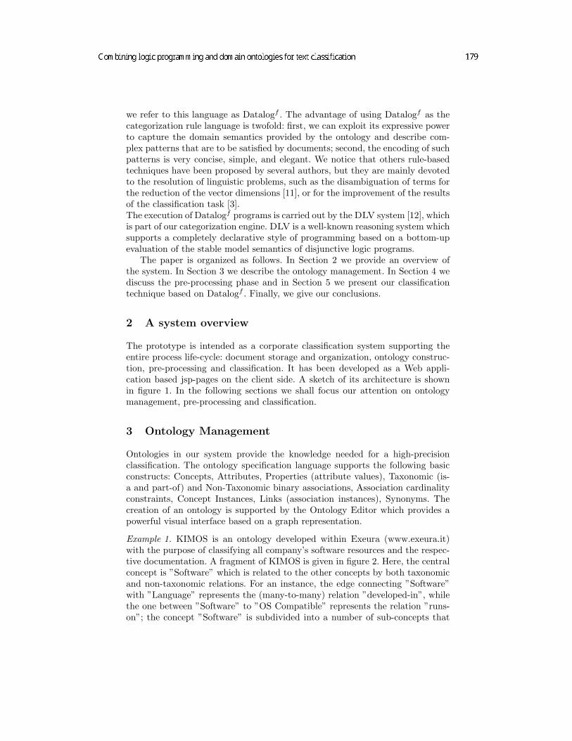
we refer to this language as Datalogf . The advantage of using Datalogf as thecategorization rule language is twofold: first, we can exploit its expressive powerto capture the domain semantics provided by the ontology and describe com-plex patterns that are to be satisfied by documents; second, the encoding of suchpatterns is very concise, simple, and elegant. We notice that others rule-basedtechniques have been proposed by several authors, but they are mainly devotedto the resolution of linguistic problems, such as the disambiguation of terms forthe reduction of the vector dimensions [11], or for the improvement of the resultsof the classification task [3].The execution of Datalogf programs is carried out by the DLV system [12], whichis part of our categorization engine. DLV is a well-known reasoning system whichsupports a completely declarative style of programming based on a bottom-upevaluation of the stable model semantics of disjunctive logic programs.

The paper is organized as follows. In Section 2 we provide an overview ofthe system. In Section 3 we describe the ontology management. In Section 4 wediscuss the pre-processing phase and in Section 5 we present our classificationtechnique based on Datalogf . Finally, we give our conclusions.

2 A system overview

The prototype is intended as a corporate classification system supporting theentire process life-cycle: document storage and organization, ontology construc-tion, pre-processing and classification. It has been developed as a Web appli-cation based jsp-pages on the client side. A sketch of its architecture is shownin figure 1. In the following sections we shall focus our attention on ontologymanagement, pre-processing and classification.

3 Ontology Management

Ontologies in our system provide the knowledge needed for a high-precisionclassification. The ontology specification language supports the following basicconstructs: Concepts, Attributes, Properties (attribute values), Taxonomic (is-a and part-of) and Non-Taxonomic binary associations, Association cardinalityconstraints, Concept Instances, Links (association instances), Synonyms. Thecreation of an ontology is supported by the Ontology Editor which provides apowerful visual interface based on a graph representation.

Example 1. KIMOS is an ontology developed within Exeura (www.exeura.it)with the purpose of classifying all company’s software resources and the respec-tive documentation. A fragment of KIMOS is given in figure 2. Here, the centralconcept is ”Software” which is related to the other concepts by both taxonomicand non-taxonomic relations. For an instance, the edge connecting ”Software”with ”Language” represents the (many-to-many) relation ”developed-in”, whilethe one between ”Software” to ”OS Compatible” represents the relation ”runs-on”; the concept ”Software” is subdivided into a number of sub-concepts that

..

Database

Document

Collector

Interface

Conceptual

Search

Textual

Document

Repository

Server Side

Client Side

Ontology Editor

Document

Collector

Pre-Processor

Module

Corpus

Manager

Repository Manager

Classification

Engine

DLV

System

Classification Manager

Corpus Interface

Ontology

Browser

Ontology Manager

Logic Rule Base

Rules Editor

Figure 1. The System Architecture

group the different instances of ”Software” into the appropriate categories. Infigure we have reported only the concept ”DB” that represents the class of soft-wares for databases. This concept is related to ”Software” by an is-a relationand it is classified into ”DBMS” and ”DB Tool”. In turn, ”DBMS” is classifiedas either ”Relational DBMS” or ”Others” (i.e., DBMS of different types). Aninstance of ”Relational DBMS” is ”MySQL” which is related to ”Unix-C” (aninstance of ”OS Compatible”) by the link ”runs-on”. 2

Once created, the user can navigate the ontology using the Ontology Browserwhich offers the following basic facilities:

– for a given concept, the user can easily explore its sub-concepts or, viceversa,collapse the underlying hierarchies

– the user can select the relationships whereby moving away from a givenconcept

– the user can filters the (possibly large) list of instances of a given concept.

Internally, an ontology is stored as a set of facts. As we will see in section 5,these facts represent an input to categorization programs.

Example 2. The internal representation of KIMOS consists of facts representing:

– concepts, e.g., concept(DB);

..

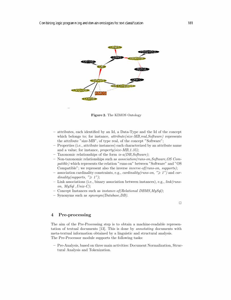
Figure 2. The KIMOS Ontology

– attributes, each identified by an Id, a Data-Type and the Id of the conceptwhich belongs to; for instance, attribute(size-MB,real,Software) representsthe attribute ”size-MB”, of type real, of the concept ”Software”;

– Properties (i.e., attribute instances) each characterized by an attribute nameand a value; for instance, property(size-MB,1.35);

– Taxonomic relationships of the form is-a(DB,Software);– Non-taxonomic relationships such as association(runs-on,Software,OS Com-

patible) which represents the relation ”runs-on” between ”Software” and ”OSCompatible”; we represent also the inverse inverse-of(runs-on, supports);

– association cardinality constraints, e.g., cardinality(runs-on, ”> 1”) and car-dinality(supports, ”> 1”);

– Link associations (i.e., binary association between instances), e.g., link(runs-on, MySql ,Unix-C);

– Concept Instances such as instance-of(Relational DBMS,MySql);– Synonyms such as synonym(Database,DB).

2

4 Pre-processing

The aim of the Pre-Processing step is to obtain a machine-readable represen-tation of textual documents [13]. This is done by annotating documents withmeta-textual information obtained by a linguistic and structural analysis.The Pre-Processor module supports the following tasks:

– Pre-Analysis, based on three main activities: Document Normalization, Struc-tural Analysis and Tokenization.

– Linguistic Analysis, based on the following steps:• Lexical Analysis: for each token, the morpho-syntactical features are

obtained (the stem and the Part of Speech - PoS). The PoS Taggingstep is based on a variant of the Brill Tagger (a rule-based Pos-Tagger[14]).

• Quantitative Analysis which provides, for a given document, informationabout the number of different tokens and stems as well as the absolutefrequency for each token and stem.

The output of the Pre-Processing phase is a set of facts representing therelevant information about the processed document. As we shall see in section5, these facts represent an input to our categorization programs.

Example 3. Consider, for example, a textual document about databases, with247 different tokens, and suppose that the third paragraph of this documentcontains the following fragment of text: ”... A database is a structured.... ”.The representation of this paragraph is like this:...word(57,’a’,’a’,’at’).word(58,’database’,’databas’,’nn’).word(59,’is’,’is’,’bez’).word(60,’a’,’a’,’at’).word(61,’structured’,’structur’,’vbn’).bold(58).par(3,57,148).tokenFrequency(’database’,13).stemFrequency(’databas’,16).numberOfTokens(247).numberOfStems(218). 2

5 Document Classification

The basic idea is that of using logic programs to recognize concepts within texts.Logic rules, indeed, provide a natural and powerful way to describe features ofdocument contents that may relate to concepts. To this end, we use the logiclanguage Datalogf [10], an extension of Datalog by aggregate functions. Themodule of our system which supports the classification process is the Classifi-cation Engine which relies on DLV system [12] for the bottom-up evaluation ofDatalogf programs.

5.1 The Datalogf language

We call Datalogf the logic language obtained by extending Datalog [9] by ag-gregate functions. A function has the form f(V ars : Conj) where f is thename (count, sum, min, max, sum) and V ars a set of variables occurring inthe conjunction Conj. Intuitively the expression V ars : Conj represents the

set of values assumed by the variables in V ars making Conj true. An aggre-gate atom is an expression of the type Lg ≤ f(V ars : Conj) ≤ Ug where Lgand Ug are positive integer constants or variables called guards. For instance,countV : a(V ) < value is an aggregate atom whose informal meaning is: thenumber of ground instances of a(V ) must be less than value. A Datalogf pro-gram is a logic program in which aggregate literals can occur in the body ofrules. Rules with aggregate atoms are required to be safe [10]. It is worth notic-ing that the result of an aggregate function can be saved by an assignment. Forinstance in the following rule h(X) : −X = #countV : a(V ), all the groundinstances of a(V ) are counted up and the value of count is assigned to X.

5.2 Categorization programs

By combining the expressive power of Datalog with that of aggregate functions,Datalogfprovides a natural and powerful tool for describing categorization ruleswithin our system. A categorization program relies on a number of predefinedpredicates, that are of two types:

1. Pre-processing predicates representing information generated by the pre-processing phase; examples of such predicates are:

word(Id, Token, Stem,PoS)title(Id, Token, Stem,PoS)

where Id represents the position of Token within the text, Stem is the stemof the token and PoS its Part-of-Speech, and

tokenFrequency(Token, Number)which represents the number of times Token occurs in the text.

2. Ontology predicates representing the domain ontology; examples of this kindof predicates are the following: instance of(I, C) (I is instance of the conceptC), synonym(C1, C2), isa(C1, C2), part of(C1, C2), association(A,C1, C2),etc..

In addition, we use the predicate relevant(D, C) to state that document D isrelevant for concept C.Now, we equip each concept C of a given ontology with a set of Datalogf rules,the categorization program PC of C, used to recognize C within a given documentD. The set of facts of PC consists of the facts representing the domain ontology(see Section 3) as well as those representing the pre-processed document (seeSection 4). The rules of PC represent conditions that are to be satisfied in orderD be considered relevant for C.

Example 4. We next provide an incremental construction of a categorization pro-gram associated with the concept ”DB” of the KIMOS ontology (see example 1).

Rules looking for keyword. We start with the following simple rules lookingfor the keyword ”DB”:

r0: t0 : −title( , ”DB”, , ).

r1: t1 : −tokenFrequency(”DB”, F ), F > a.

In rule r0 above, the predicate t0 is true if ”DB” occurs in the title, whilet1 in r1 is true if the frequency F of the token ”DB” is greater than a givenconstant a.We can now refine our keyword search by exploiting synonyms; for instance, wecan restate r0 as

r0: t0 : −title( , X, , ), synonym(X, ”DB”).

and replace r1 by the following two rules:

r2: t2(X, F ) : −synonym(X, ”DB”), word( , X, , ), tokenFrequency(X,F ).

r3: t3 :- F1 = #sumF,X : t1(F,X), F1 > a.

Rule r2 above ”evaluates”, for the concept ”DB” and each of its synonyms,the respective frequency F ; rule r3, in turn, determines the total number F1 oftimes the concept ”DB” and each of its synonyms appears in the text (this isperformed by the aggregate function sum).

Rules looking for terms. Using the next rules we look for the term ”structureddata” within the document:

r4 : t4(I) :- word(I, ”structured”, , ), word(J, ”data”, , ), J = I + 1.

r5 : t5(F ) :- F = #countI : t5(I).

We may relax the above condition, requiring the words ”structured” and ”data”to be found, in the specified order, within a distance of at most 5 words insidethe same paragraph:

r6 : t6(I) :- word(I, ”structured”, , ), word(J, ”data”, , ), J > I,L = J − I, L <= 5, sameParagraph(I, J).

r7: sameParagraph(I, J) :- par(Id, Init, F in), I >= Init, J <= Fin.

r8 : t8(F ) :- F = #countI : t7(I).

Rule r8 above counts the number of times the searched term occurs in the sameparagraph.

Rules matching expressions. Next we write rules to recognize, within a para-

graph, an expression of the following type: a verb with stem ”store”, followedby a name having ”tabl” or ”relat” as its stem (i.e., we are trying to recognizesentences such as ”data are stored within tables...”).

r9 : t9(I) :- word(I, , ”store”, ”vb”), word(J, , ”tabl”, ), sameParagraph(I, J).

r10 : t10(I) :- word(I, , ”store”, ”vb”), word(J, , ”relat”, ), sameParagraph(I, J).

r11 : t11(F ) :- F = #countI : t9(I).

Rules exploiting the ontology knowledge. We can improve the precision of theclassification process by using the underlying domain ontology. For instance, ifa document talks about some specific instances of the concept ”db”, such asOracle, Access, etc. (note that an instance of ”relational DBMS”, which is asub-concept of ”db”, is also an instance of ”DB”), it is quite obvious consideringthe document as pertinent to the concept ”db”. So, we write the following rules:

r12 : t12(I, F ) :- instance of(”DB”, I), tokenFrequency(I, F ).

r13: t13(N) :- N = #countI : t11(I, ).

r14 : t14(F ) :- F = #sumF1, I : t11(I, F1).

r15 : t15(T ) :- T = #countI : instance of(I, ”DB”).

where: r12 provides the number of occurrences of each instance of ”db” in thedocument; r13 counts the number of distinct instances of ”db”; r14 provides thetotal number of instances (duplicated included) of ”db” and r15 gives the num-ber of instances of ”db” in the ontology. Finally, the rule

r16 : t16(K, L) :- t13(N), t14(F ), t15(T ),K = N/T, L = F/N.

expresses a measure, in terms of K (the fraction of the instances of ”db” thatare cited within the document) and L (which takes into account the fact thateach instance might be cited several times), of the presence into the documentof words representing instances of the concept ”db”. 2

As we have mentioned before, we use DLV as the categorization engine inour system. DLV is a very powerful system for the bottom-up evaluation ofdisjunctive logic programs extended by a number of constructs (Datalogf is asubset of the DLV language). It is used in many real applications where efficiencyis a strong constraint.The evaluation strategy of categorization programs is based on the following twoobservations:

– there are documents that are straightforward to classify, i.e., for which simplekeyword-based rules (like r1 − r2 above) are enough; suppose, for instance,

that the word ”db” is contained in the title or it occurs frequently throughoutthe text; in such cases we can confidently classify the document at handas relevant for the given concept only by using few simple rules (like r1

and r2) and forgetting of the remaining ones occurring in the rest of thecategorization program;

– a deeper semantic analysis is needed only in case of documents that aredifficult to classify because concepts do not appear explicitly; to this end,the execution of more complex rules (for instance, rules trying to matchcomplex expressions) is required.

Now, the implementation of the above evaluation strategy proceeds, roughlyspeaking, as follows: we structure the categorization program PC , associated tothe concept C, into a number of components, say, c1, ..., cn. Each componentgroups rules performing some specific retrieval task, such as word-based search,term matching, etc., of increasing semantic complexity – that is, each componentis capable to recognize texts that are possibly inaccessible to the ”previous” ones.Given a document D, the evaluation of PC (w.r.t. D) starts from c1 (the ”lowest”component) and, as soon as a component ci, 1 ≤ i ≤ n, is ”satisfied” (by D),the process stops successfully – i.e., D is recognized to be relevant for C and thefact relevant(D,C) is stated to be true; if no such a component is found, theclassification task fails.

5.3 Ontology-driven Classification Strategy

Let D be a document that has to be classified w.r.t. an ontology O. As we haveseen in the previous subsection, each concept C of O is equipped with a suitablecategorization program PC whose evaluation determines whether D is relevantfor C or not. An exhaustive approach would require to ”prove” D w.r.t. thecategorization program of each concept of O, and this could result in a ratherheavy computation. However, we can drastically reduce the ”search space” if weadopt an ontology-driven classification technique which exploits the presence oftaxonomic hierarchies. This technique is based on the principle that if a docu-ment is relevant for a concept then it is so for all of its ancestors within an is-ataxonomy (unless the contrary is explicitly stated). This principle is expressedby the following recursive rule:

relevant(D, X) : −relevant(D, Y ), isa(Y, X)

As an example, if a document is relevant for the concept ”Relational DBMS” ofthe KIMOS ontology, then it is so for the concepts ”DBMS”, ”DB” and ”Soft-ware”. If we want to exclude the latter, we simply write:

relevant(D, X) : −relevant(D, Y ), isa(Y, X), X <> ”Software”.

The above inheritance principle suggests us a classification strategy where con-cepts within a sub-class hierarchy are processed in a bottom-up fashion. As soon

as D is found to be relevant for a concept C in the hierarchy H, it is not anymore processed w.r.t. any of the ancestors of C in H. The relevance associationof D to the ancestors of C is automatically performed by the above recursiverule.

6 Conclusion

We have presented a prototypical text classification system which relies on acombined use of ontologies and logic programming. The former are used to rep-resent the domain knowledge, the latter to recognize concepts within texts. Tothis end, each concept of an ontology is equipped with a categorization pro-gram, i.e., a logic program written in Datalogf – an extension of Datalog byaggregate functions. A categorization program is designed to discover complexpatterns within texts using the knowledge provided by the underlying ontology.The classification process is ontology-driven and, as a result, provides a relation-ship between concepts and documents. The categorization engine is based onthe logic programming system DLV.So far, we have carried out a number of preliminary tests which seem to be verypromising in terms of efficiency even on large documents. For an instance, we canclassify a document of over 70000 words w.r.t. a Kimos Ontology (7 concepts)in 0.51 seconds. Further experimentation is currently being performed.Current work is concerned with the extension of Datalogf with external func-tions for the efficient execution of tasks such as stemming, substring matching,etc.

References

1. Ciravegna: (LP)2, an Adaptive Algorithm for Information Extraction from Web-related Texts. In: Proc. IJCAI-2001 Work. on Adaptive Text Extraction and Min-ing. (2001)

2. Riloff: A Case Study in Using Linguistic Phrases for Text Categorization on theWWW. In: AAAI/ICML Work.Learning for Text Categorization. (2001)

3. Cohen: Text categorization and relational learning. In: Proc. of ICML-95, 12thInt. Conference on Machine Learning. (1995)

4. Dıaz, A., Buenaga, M., Urena, L., Garcıa-Vega, M.: Integrating linguistic resourcesin an uniform way for text classification tasks. In: Proc. of LREC-98, 1st Int.Conference on Language Resources and Evaluation. (1998) 1197–1204

5. Hsu: Classification algorithms for NETNEWS articles. In: Proc. of CIKM-99, 8thACM Int. Conference on Information and Knowledge Management. (1999) 114–121

6. Brank, J., Grobelnik, M., Milic-Frayling, N., Mladenic, D.: Feature selection usingsupport vector machines. In: Proc. of the 3rd International Conference on DataMining Methods and Databases for Engineering, Finance, and Other Fields. (2002)

7. Decker, S., Erdmann, M., Fensel, D., Studer, R. In: Ontobroker: Ontology BasedAccess to Distributed and Semi-Structured Information. Proc. of DS-8. KluwerAcademic Publ (1999) 351–369

8. Fensel: OIL: An ontology infrastructure for the semantic web. IEIS 16 (2001)38–45

9. Ullman: Principles of Database and Knowledge-Base Systems, Rockville (Md.)(1988)

10. Dell’Armi, T., Faber, W., Ielpa, G., Leone, N., Pfeifer, G.: Aggregate Functionsin Disjunctive Logic Programming: Semantics, Complexity, and Implementationin DLV. In: Proc. IJCAI 2003, Acapulco, Mexico, Morgan Kaufmann Publishers(2003)

11. Paliouras: Learning rules for large vocabulary word sense disambiguation. In:Proc. of IJCAI-99. (1999) 674–679

12. Faber, W., Pfeifer, G.: DLV homepage (since 1996) http://www.dlvsystem.com/.13. Yang: A comparative study on feature selection in text categorization. In: Inter-

national Conference on Machine Learning, ACL (1997) 412–42014. Brill: Tranformation-based error-driven learning and natural language processing:

A case study in part of speech tagging. In: Computational Linguistics. (1995)543–565

Ontological encapsulation of many-valued logic

Zoran Majkic

Dipartimento di Informatica e Sistemistica, University of Roma “La Sapienza”Via Salaria 113, I-00198 Rome, Italy

majkic@dis.uniroma1.ithttp://www.dis.uniroma1.it/∼ majkic/

Abstract. Large databases obtained by the data integration of different sourcedatabases can be incomplete and inconsistent in many ways. The classical logicis not the appropriate formalism for reasoning about inconsistent databases. Cer-tain local inconsistencies should not be allowed to significantly alter the intendedmeaning of such logic programs. The variety of semantical approaches that havebeen invented for logic programs is quite broad. In particular we are interestedfor many-valued logics with negation, based on bilattices. We present a 2-valuedlogic, based on an Ontological Encapsulation of Many-Valued Logic Program-ming, which overcome some drawbacks of the previous research approaches inmany-valued logic programming. We defined a Model theory for Herbrand in-terpretations of ontologically encapsulated logic programs, based on a semanticreflection of the epistemic many-valued logic.

1 Introduction to Many-valued logic programming

Semantics of logic programs are generally based on a classical 2-valued logic by meansof stable models, [1,2]. Under these circumstances not every program has a stablemodel. Three-valued, or partial model semantics had an extensive development for logicprograms generally, [3,4]. Przymusinski extended the notion of stable model to allow3-valued, or partial, stable models, [5], and showed every program has at least one par-tial stable model, and the well-founded model is the smallest among them, [6]. Onceone has made the transition from classical to partial models allowingincompleteinfor-mation, it is a small step to also allow models admittinginconsistentinformation. Doingso provides a natural framework for the semantic understanding of logic programs thatare distributed over several sites, with possibly conflicting information coming fromdifferent places. As classical logic semantics decrees that inconsistent theories have nomodels, classical logic is not the appropriate formalism for reasoning about inconsistentdatabases: certain ”localizable” inconsistences should not be allowed to significantly al-ter the intended meaning of such databases.So far, research in many-valued logic programming has proceeded along different di-rections:Signedlogics [7,8] andAnnotatedlogic programming [9,10] which can beembedded into the first,Bilattice-basedlogics, [11,12], andQuantitative rule-sets,[13,14]. Earlier studies of these approaches quickly identified various distinctions be-tween these frameworks. For example, one of the key insights behind bilattices wasthe interplay between the truth values assigned to sentences and the (non classic) no-tion of implication in the language under considerations. Thus, rules (implications) had

weights (or truth values) associated with them as a whole. The problem was to studyhow truth values should be propagated ”across” implications. Annotated logics, on theother hand, appeared to associate truth values with each component of an implicationrather than the implication as a whole. Roughly, based on the way in which uncertaintyis associated with facts and rules of a program, these frameworks can be classified intoimplication based(IB) andannotation based(AB).In the IB approach a rule is of the formA←α B1, .., Bn , which says that the certaintyassociated with the implication isα. Computationally, given an assignmentI of logicalvalues to theBis, the logical value ofA is computed by taking the ”conjunction” oflogical valuesI(Bi) and then somehow ”propagating” it to the rule headA.In the AB approach a rule is of the formA : f(β1, .., βn) ← B1 : β1, ..., Bn : βn ,which asserts ”the certainty of the atomA is least (or is in)f(β1, .., βn), whenever thecertainty of the atomBi is at least (or is in)βi, 1 ≤ i ≤ n”, wheref is an n-ary com-putable function andβi is either constant or a variable ranging over many-valued logicvalues.The comparison in [15] shows:1- while the way implication is treated on the AB approach is closer to the classicallogic, the way rules are fired in the IB approach has definite intuitive appeal.2- the AB approach is strictly more expressive than IB. The down side is that queryprocessing in the AB approach is more complicated, e.g. the fixpoint operator is notcontinuous in general, while it is in the IB approaches.3- the Fitting fixpoint semantics for logic programs, based exclusively on a bilattice-algebra operators, suffer two drawbacks: the lack of the notion of tautology (bilatticenegation operator is anepistemicnegation) leads to difficulties in defining proof proce-dures and to the need for additional complex truth-related notions as ”formula closure”;there is an unpleasant asymmetry in the semantics of implication (which is strictly 2-valued) w.r.t. all other bilattice operators (which produce any truth value from the bi-lattice) - it is a sign that strict bilattice language is not enough expressive for logicprogramming, and we need some reacher (different) syntax for logical programming.From the above points, it is believed that IB approach is easier to use and is moreamenable for efficient implementations, but also annotated syntax (but with IB seman-tics) is useful to overcome two drawbacks above: the syntax of new encapsulated many-valued logic (in some sense ’meta’-logic for a many-valued bilattice logic) will be 2-valued and can be syntactically seen as a kind of very simple annotated syntax. Thusthe implication (and classical negation also), not present in a bilattice algebra operators,will have a natural semantic interpretation in this enriched framework.In [10] it is shown how the Fitting’s 3-valued bilattice logic can be embedded intoan Annotated Logic Programming which is computationaly very complex. The aim ofthis work is (1) to extend the Fittihg’s fixpoint semantics to deal with inconsistenciesalso, and (2) to define the notion of a model for such many-valued logic programs bysome kind of ’minimal’ (more simple and less computationally expensive than APC)logic. In order to respond to these questions we (1) introducebuilt-in predicatesin theheads of clauses, and (2)encapsulatethe ’object’ epistemic many-valued logic pro-grams into 2-valued ’meta’ ontological logic programs. We argue that such logic willbe good framework for supporting the data integration systems with key and foreign

key integrity constraints with incomplete and inconsistent source databases, with lesscomputation complexity for certain answers to conjunctive queries [16,17].The plan of this paper is the following: Section 2 introduce the Belnap’s bilattice con-cepts and the particular 4-valued version,B4, used in this paper. In Section 3 is pre-sented an inference framework for a 4-valued bilattice based logic, particularly forderivation ofpossiblefacts (w.r.t. true and false facts as in 3-valued strong Kleene’slogic) and is given a representation theorem for this 4-valued logic. In Section 4 isdeveloped conceptual framework for encapsulation of this epistemic ’object’ 4-valuedlogic into an ontological ’meta’ 2-valued logic by mean ofsemantic reflection. More-over, is given the definition for a 4-valued implication useful for inconsistent databasesand an example where inconsistency is managed by clauses with built-in predicate in ahead. Finally, Section 5 defines the syntax and themodel theoreticHerbrand semanticsfor the ontological encapsulation of many-valued logic programs.

2 Many-valued epistemic logic based on a Bilattice

In [18], Belnap introduced a logic intended to deal in a useful way with inconsis-tent or incomplete information. It is the simplest example of a non-trivial bilattice andit illustrates many of the basic ideas concerning them. We denote the four values ast, f,ᵀ,⊥, wheret is true, f is false, ᵀ is inconsistent (both true and false) orpos-sible, and⊥ is unknown. As Belnap observed, these values can be given two naturalorders:truth order,≤t, andknowledgeorder,≤k, such thatf ≤t ᵀ ≤t t, f ≤t⊥≤t t,and⊥≤k f ≤k ᵀ, ⊥≤k t ≤k ᵀ. This two orderings define corresponding equivalences=t and=k. Thus any two membersα, β in a bilattice are equal,α = β, if and only if(shortly ’iff’ ) α =t β andα =k β.Meet and join operators under≤t are denoted∧ and∨; they are natural generalizationsof the usual conjunction and disjunction notions. Meet and join under≤k are denoted⊗ (consensus, because it produces the most information that two truth values can agreeon) and⊕ (gullibility , it accepts anything it’s told), such that hold:f ⊗ t =⊥, f ⊕ t = ᵀ, ᵀ∧ ⊥= f andᵀ∨ ⊥= t.There is a natural notion of truth negation, denoted∼, (reverses the≤t ordering, whilepreserving the≤k ordering): switchingf and t, leaving⊥ andᵀ, and correspondingknowledge negation, denoted− (reverses the≤k ordering, while preserving the≤t or-dering), switching⊥ andᵀ, leavingf and t. These two kind of negation commute:− ∼ x =∼ −x for every memberx of a bilattice.It turns out that the operations∧,∨ and∼, restricted tof, t,⊥ are exactly those ofKleene’s strong 3-valued logic. Any bilattice〈B,≤t,≤k〉 is:1. Interlaced, if each of the operations∧,∨,⊗ and⊕ is monotone with respect to bothorderings (for instance,x ≤t y impliesx⊗z ≤t y⊗z , x ≤k y impliesx∧z ≤k y∧z).2. Infinitarily interlaced, if it is complete and four infinitary meet and join operationsare monotone with respect to both orderings.3. Distributive, if all 12 distributive laws connecting∧,∨,⊗ and⊕ are valid.4. Infinitarily distributive, if it is complete and infinitary, as well as finitary, distributivelaws are valid. (Note that a bilattice iscompleteif all meets and joins exist, w.r.t. bothorderings. We denote infinitary meet and join w.r.t.≤t by

∧and

∨, and by

∏and

∑

for the≤k ordering; for example, the distributive law for⊗ and∧

may be given byx⊗

∧i yi =

∧i(x⊗ yi)).

A more general information about bilattice may be found in [19]: he also definesexactmembers of a bilattice, whenx = −x (they are 2-valued consistent), andconsistentmembers, whenx ≤k −x (they are 3-valued consistent), but a specific 4-valued consis-tence will be analyzed in the following paragraphs.The Belnap’s 4-valued bilattice is infinitary distributive. In the rest of this paper we de-note byB4 a special case of the Belnap’s bilattice. In this way we consider thepossiblevalue as weak true value and not as inconsistent (that is true and false together). Wehave more knowledge for ground atom with such value, w.r.t. the true ground atom,because we know also that if we assign the true value to such atom we may obtain aninconsistent database.

3 Representation theorem

Ginsberg [11] defined a world-based bilattices, considering a collection of worldsW ,where by world we mean some possible way of things might be, and where[U, V ] isa pair of subsets ofW which express truth of some sentencep, with ≤t,≤k truth andknowledge preorders relatively, as follows:1.U is a set of worlds wherep is true,V is a set of worlds wherep is false,P = U

⋂V

is a set wherep is inconsistent (both true and false), andW − (U⋃V ) is a set wherep

is unknown.2. [U, V ] ≤t [U1, V1] iff U ⊆ U1 and V1 ⊆ V3. [U, V ] ≤k [U1, V1] iff U ⊆ U1 and V ⊆ V1

Such definition is well suited for the 3-valued Kleene logic, but for the 4-valued logicused to overcome ”localizable” inconsistencies it is not useful, mainly for two follow-ing reasons:1. Theinconsistent(both true and false) top knowledge value in the Belnap’s bilatticecan’t be assigned to sentences, otherwise we will obtain an inconsistent logic theory;because of that consistent logics in this interpretation can have only three remainingvalues. Thus we interpret it aspossiblevalue, which will be assigned to mutually incon-sistent sentences, and we obtain possibility to have consistent 4-valued logic theories inorder to overcome such inconsistencies.2. Let denote byT = U − P , F = V − P , whereP is a set of worlds wherep has apossible logic value. Then we obtain that[U, V ] ≤t [U1, V1] also whenT ⊃ T1, whichis in contrast with our intuition. Consequently, we adopt a triple[T, P, F ] of mutuallydisjoint subsets ofW to express truth of some sentencep (W − T

⋃P

⋃F are worlds

wherep is unknown), with the following definition for their truth and knowledge orders:2.1 [T, P, F ] ≤t [T1, P1, F1] iff T ⊆ T1 andF1 ⊆ F2.2 [T, P, F ] ≤k [T1, P1, F1] iff T ⊆ T1, P ⊆ P1 andF ⊆ F1.Let us try now to rendermore rationalthese two intuitions described above. In orderto obtain a new bilattice abstraction rationality, useful to manage logic programs withpossible ’localizable’ inconsistencies, we need to consider more deeply thefundamentalphenomenain such one framework. In the process of derivation of new facts, for a givenlogic program, based on the ’immediate consequence operator’, we have the following

three truth transformations for ground atoms in a Herbrand base of such program:1. When ground atom pass fromunknownto true logic value, without generating incon-sistence. Let denote this action by↑1:⊥ t. The preorder of this 2-valued sublatticeof B, L1 = ⊥, t, defined by the direction of this transformation, ’truth increasing’,is ≤1 ≡ ≤t. The meet and join operators for this lattice are∧,∨ respectively. It is alsoknowledge increasing.2. When some ground atom, try to pass from unknown to true/false value, generating aninconsistency, then is applied theinconsistency repairing, that is thetrue value of theliteral of this atom, in a body of a violated clause with built-in predicate, is replaced bypossiblevalue. Let denote this action by↑2: t ᵀ. The preorder of this 2-valued sub-lattice ofB, L2 = t,ᵀ, defined by the direction of this transformation, ’knowledgeincreasing’. The meet and join operators for this lattice, w.r.t. this ordering are⊗,⊕respectively. Notice that this transformationdoes not changethe truth ordering becausethe ground atom pass from unknown to possible value.3. When ground atom pass fromunknownto falselogic value, without generating incon-sistence. Let denote this action by↑3:⊥ f . The preorder of this 2-valued sublatticeof B, L3 = ⊥, f, defined by the direction of this transformation, ’falsehood increas-ing’ (inverse of ’truth increasing’), is≤3 ≡ ≤−1

t . The meet and join operators for thislattice are∨,∧ respectively. It is also knowledge increasing.Thus, any truth transformation in some multi-valued logic theory (program) can be seenas composition of these three orthogonal dimensional transformations,i.e. by triples (ormulti-actions), [a1, a2, a3], acting on the idle (default) state[⊥, t,⊥]; for instance themulti-action [ , , ↑3], composed by the singe action↑3, applied to the default stategenerates the ”false” state[⊥, t, f ]. The default state[⊥, t,⊥] in this 3-dimensionalspace has role as unknown value for single-dimensional bilattice transformations, thatis it is a ”unknown” state. Consequently, we define this space of states by the cartesianproduct of single-dimensional lattices,L1 × L2 × L3, composed by triples[x, y, z],x ∈ L1 = ⊥, t, y ∈ L2 = t,ᵀ andz ∈ L3 = ⊥, f.

Definition 1. By L1 L2 L3 we mean the bilattice< L1 × L2 × L3,≤Bt ,≤B

k >where, given anyX = [x, y, z], andX1 = [x1, y1, z1]:1. Considering that the second transformation does not influence the truth ordering,X ≤B

t X1 if x ≤1 x1 andz ≤3 z1 , i.e., if x ≤t x1 andz ≥t z12. Considering that all three transformations are knowledge increasing, we haveX ≤B

k X1 if x ≤k x1 andy ≤k y1 andz ≤k z13.X ∧B X1 =def [(x ∧1 x1, y ∧1 y1), z ∧3 z1] = [x ∧ x1, y ∧ y1, z ∨ z1]4.X ∨B X1 =def [x ∨1 x1, (y ∨3 y1, z ∨3 z1)] = [x ∨ x1, y ∧ y1, z ∧ z1]5.X ⊗B X1 =def [x⊗ x1, y ⊗ y1, z ⊗ z1]6.X ⊕B X1 =def [x⊕ x1, y ⊕ y1, z ⊕ z1]

These three bilattice transformations can be formally defined by lattice homomor-phisms.

Proposition 1 The following three lattice homomorphisms defines the 3-dimensionaltruth transformations:1. Truth dimension, θ1 = ∨ ⊥: (B,∧,∨,⊗,⊕)→ (L1,∧1,∨1,⊗,⊕),with ∧1 = ∧, ∨1 = ∨. This is a strong positive transformation, which transforms

falsehood into unknown and possibility in truth.2. Possibility dimension,θ2 = ∨ ∼ ∨ ᵀ : (B,⊗,⊕) → (L2,⊗,⊕). This is a weakknowledge transformation which transform unknown into possibility.3. Falsehood dimension,θ3 = ∧ ⊥: (B,∨,∧,⊗,⊕)→ (L3,∧3,∨3,⊗,⊕),with∧3 = ∨, ∨3 = ∧. This is a strong negative transformation, which transforms truthinto unknown and possibility into falsehood.We define the following two mappings between Belnap’s and its derived bilattice:Dimensional partitioning: θ =< θ1, θ2, θ3 >: B → L1 L2 L3 andCollapsing:ϑ : L1 L2 L3 → B, such thatϑ(x1, x2, x3) =def (x1 ⊕ x3) ∧ x2.

These three lattice homomorphisms preserves the bilattice structure ofB into the spaceof statesL1 L2 L3. That is we have that (′ ′ represents no action)θ(⊥) = [ , , ]([⊥, t,⊥]) = [⊥, t,⊥], unknown stateθ(f) = [ , , ↑3]([⊥, t,⊥]) = [⊥, t, f ], false stateθ(t) = [↑1, , ]([⊥, t,⊥]) = [t, t,⊥], true stateθ(ᵀ) = [↑1, ↑2, ↑3]([⊥, t,⊥]) = [t,ᵀ, f ], possible state.Notice that the multi-action[↑1, ↑2, ↑3] represents two cases for repairing inconsis-tencies: first, when unknown value of some ground atom tries to become true (action↑1) but makes inconsistency, thus is applied also action↑2 to transform it into possiblevalue; second, when unknown value of some ground atom tries to become false (action↑3) but makes inconsistency, thus is applied also action↑2 to transform it into possiblevalue. Notice that the isomorphism between the set of states and the set of multi-actions[a1, a2, a3] | a1 ∈ ↑1, , a2 ∈ ↑2, , a3 ∈ ↑3, defines thesemanticsto thebilatticeL1 L2 L3.

Proposition 2 Let Imθ ⊆ L1 L2 L3 be the bilattice obtained by image of Di-mensional partitioning. It has also unary operators:Negation, ∼B = θ ∼ ϑ , and conflation, −B = θ − ϑ.

It is easy to verify thatϑ θ = idB is an identity onB, and thatϑ is surjective withθ ϑ = idImθ. The negation∼B preserves knowledge and inverts truth ordering and∼B∼B X = X; the conflation−B preserves truth and inverts knowledge orderingand−B −B X = X; and holds the commutativity∼B −B = −B ∼B . ( for example,∼B −B = θ ∼ ϑθ−ϑ = θ ∼ idB−ϑ = θ ∼ −ϑ = θ− ∼ ϑ = θ−ϑθ ∼ ϑ = −B ∼B).So, we obtain that, for anyX = [x, y, z], hold ∼B X =def [∼ z, y,∼ x] and−BX =def [θ1(−z), θ2(−ϑ(X)), θ3(−x)].Theorem 1. (Representation theorem) IfB is a 4-valued distributive lattice then thereare its distributive sublattices,L1, L2, L3, such thatB is isomorphic to the sublatticeof L1 L2 L3 defined by image of Dimensional partitioningImθ . Moreover thefollowing diagram (on the left) of bilattice homomorphisms commute

L1 L2 L3θϑ- Imθ

'π1×π3 - L1 L3 L2(possibility)

@@

@@

ϑR

'3

B

'4

?(falsehood)L3

θ3 B

θ2

6

θ1- L1(truth)

where'π1×π3 is a projection isomorphism,'3 is the isomorphism (restriction ofϑ tothe projectionL1L3) of Fitting’s representation Th. [20] valid for a 3-valued logics,and'4 is new 4-valued isomorphism (restriction ofϑ to Imθ , and inverse toθ).If B has negation and conflation operators that commute with each other, they are pre-served by all isomorphisms of the right commutative triangle.

Proof. It is easy to verify that all arrows are homomorphisms (w.r.t. binary bilatticeoperators). The following table represents the correspondence of elements of these bi-lattices defined by homomorphisms:

Multi− actions L1 L2 L3 Imθ L1 L3 B[ , , ] [⊥, t,⊥] [⊥, t,⊥] [⊥,⊥] ⊥[ , ↑2, ] [⊥,ᵀ,⊥][ , , ↑3] [⊥, t, f ] [⊥, t, f ] [⊥, f ] f[ , ↑2, ↑3] [⊥,ᵀ, f ][↑1, , ] [t, t,⊥] [t, t,⊥] [t,⊥] t[↑1, ↑2, ] [t,ᵀ,⊥][↑1, ↑2, ↑3] [t,ᵀ, f ] [t,ᵀ, f ] [t, f ] ᵀ[↑1, , ↑3] [t, t, f ]

Let prove, for example, that the isomorphismθ : B → Imθ preserves negation andconflation: ∼B θ(x) = θ ∼ ϑθ(x) = θ ∼ idB(x) = θ(∼ x) , and−Bθ(x) = θ − ϑθ(x) = θ − idB(x) = θ(−x).

4 Semantic reflection of the epistemic logic

We assume that the Herbrand universe isΓU = Γ⋃Ω, whereΓ is ordinary domain

of database constants, andΩ is an infinite enumerable set of marked null values,Ω =ω0, ω1, ...., and for a given logic programP composed by a set of predicate andfunction symbols,PS , FS respectively, we define a set of all terms,TS , and its subsetof ground termsT0, then atoms are defined as:AS = p(c1, .., cn) | p ∈ PS , n = arity(p) and ci ∈ TSThe Herbrand base,HP , is the set of all ground (i.e., variable free) atoms. A (ordinary)Herbrand interpretation is a many-valued mappingI : HP → B. If P is a many-valuedlogic program with the Herbrand baseHP , then the ordering relations and operationsin a bilatticeB4 are propagated to the function spaceBHP

4 , that is the set of all Herbrandinterpretations (functions),I = vB : HP → B4, as follows:

Definition 2. Ordering relations are defined on the Function spaceBHP4 pointwise, as

follows: for any two Herbrand interpretationsvB , wB ∈ BHP4

1. vB ≤t wB if vB(A) ≤t wB(A) for all A ∈ HP .2. vB ≤k wB if vB(A) ≤k wB(A) for all A ∈ HP .3.∼ vB is the interpretation such that(∼ vB)(A) =∼ (vB(A)).4.−vB is the interpretation such that(−vB)(A) = −(vB(A)).

It is straightforward [19] that this makes a function spaceBHP4 itself a complete infini-

tary distributive bilattice.

One of the key insights behind bilattices [11,12] was the interplay between the truthvalues assigned to sentences and the (non classic) notion ofimplication. The problemwas to study how truth values should be propagated ”across” implications. In [21] isproposed the following IB based approach to the ’object’ 4-valued logic programming,which extends the definition given for a 3-valued logic programming [5]:

Definition 3. LetPB be the set of built-in predicates. The valuation,vB : HP → B4, isextended to logic implication of a ground clausep(c)← B , whereB = B1 ∧ ..∧Bn,as follows:vB(B → p(c)) = t , iff vB(p(c)) ≥t vB(B) or (vB(B) = ᵀ and p ∈ PB)

Inconsistency acceptance: if p ∈ PB is a built-in predicate, this clause is satisfied alsowhen vB(p(c)) = f and vB(B) = ᵀ . This principle extends the previous definitionof implication based only on truth ordering.In order to obtain such many-valued definition, which generalize the 2-valued definitiongiven above we will consider the conservative extensions of Lukasiewicz’s and Kleene’sstrong 3-valued matrices (where third logic value⊥ is considered as unknown). So weobtain the following matrix,f← : B × B → B, for implication (α = t andα =⊥ forLukasiewicz’s and Kleene’s case, respectively):

→ t ⊥ ᵀ ft t ⊥ ᵀ f⊥ t α ᵀ ⊥ᵀ t t t tf t t t t

For our purpose we assume the Lukasiewicz’s extension, i.e.α = t, in order to havea tautologya ← a for any formulaa, and also to guarantee the truth of a clause (im-plication) p(c) ← B , whenevervB(p(c)) ≥t vB(B) , as used in fixpoint semanticsfor ’immediate consequence operators’. Such conservative extensions are based on thefollowing observation: the problem to study how the truth values should be propagated”across” implications can be restricted only totrue implications ( in fact we don’t useimplications when are not true, because the ’immediate consequence operator’ derivesnew facts only fortrueclauses, i.e. when implication is true).Example 1: The built-in predicates(ex, =,≤,≥, ..) may be used for integrity con-straints: letp(x, y) be a predicate and we define the key-constraint for attributes inx by(y = z) ← p(x, y), p(x, z), where the atomy = z is based on the built-in predicate′ =′. Let consider a program : p(x, y)← r(x, y) , (y = z)← p(x, y), p(x, z)wherer is a source database relation with two tuples,(a, b), (a, c), p is a virtual rela-tion of this database with key constraint, andx, y, z are object variables. The built-inpredicates have the same prefixed extension inall models of a logic program, and thattheir ground atoms aretrue or false. If we assume that,r(a, b), r(a, c) are true, thensuch facts are mutually inconsistent forp because of key constraint (b = c is false).Thus, only one of them may be true in any model of this logic program, for exampler(a, b) . So, if we assign the ’possible’ valueTto r(a, c) (or to both of them), we obtainthat the clause(b = c) ← p(a, b), p(a, c), thanks to theinconsistency acceptance, issatisfied.

EachHerbrand interpretationis a valuation. Valuations can be extended to maps fromthe set of all ground (variable free) formulas toB in the following way:

Definition 4. LetPS be the set of all predicate symbols (PB ⊆ PS is a subset of built-in predicates), e the special (error) singleton, andI : HP → B be a many-valuedHerbrand interpretation. A valuationI determines:1. A Generalized interpretation mappingI : PS ×

⋃i≤ω T i

0 → B⋃e, such that for

anyc = (c1, .., cn) ∈ T n0 , I(p, c) = I(p(c)) iff arity(p) = n ; e otherwise.

2. A unique valuation map, also denotedvB : L → B, on the set of all ground formulasL, according to the following conditions:2.1.vB(∼ X) =∼ vB(X)2.2.vB(X Y ) = vB(X) vB(Y ), where ∈ ∧,∨,⊗,⊕ ←3. A truth assignmentuB : L → B will be called an extension of a truth assignmentvB if uB(ψ) ≥k vB(ψ) for all ψ ∈ L. If uB is an extension ofvB , we will writeuB ≥k vB .

The ’object’ many-valued logic is based on four bilattice values which areepistemic.Sentences are to be marked with some of these bilattice logic values, according as towhat the computer has been told; or, with only a slight metaphor, according to what itbelieves or knows. Of course these sentenceshavealso Frege’s ontological truth-values(true and false), independently of what the computer has been told: we want that thecomputer can use also these ontological ’meta’ knowledge. Let, for example, the com-puter believes that the sentencep has a valueT (possible); then the ’meta’ sentence,”I(computer) believe thatp has a possible value” isontologically true. The many-valuedencapsulation, defined as follows, is just the way to pass from the epistemic (’object’)many-valued logic into ontological (’meta’) 2-valued logic.Such encapsulation is characterized by having capability forsemantic-reflection: intu-itively, for each predicate symbol we need some function whichreflectsits logic seman-tic over a domainΓU . Let introduce also the set of functional symbolsκp over a domainΓU in our logical language in order to obtain an enriched logical language where wecan encapsulate the ’object’ (ordinary) many-valued logic programming. Such set offunctional symbols will be derived from the following Bilattice-semantic mappingK:

Definition 5. A semantic-reflection is a mappingK : PS → (B⋃e)

⋃i≤ωT i0 , and

we denote shortlyκp = K(p) :⋃

i≤ω T i0 → B

⋃e, p ∈ PS , such that for any

c = (c1, .., cn) ∈ T n0 , holds: κp(c) = e iff arity(p) 6= n.

If p is a built-in predicate, then a mappingκp is uniquely defined by: for anyc ∈T n

0 , n = arity(p), holds thatκp(c) = t if p(c) is true; f otherwise.

5 Ontological encapsulation programming language

The many-valued ground atoms of a bilattice-based logical languageLB can be trans-formed in ’encapsulated’ atoms of a 2-valued logic in the following simple way: theoriginal (many-valued) fact that the ground atomA = p(c1, .., cn), of the n-ary pred-icate p, has an epistemic valueα = κp(c1, .., cn) in B4, we transform in encapsu-lated atompA(c1, .., cn, α) with meaning ”it is true thatA has a valueα”. Indeed,

what we do is toreplacethe original n-ary predicatep(x1, .., xn) with n+1-ary predi-catepA(x1, .., xn, α), with the added logic-attributeα. It is easy to verify that for anygiven many-valued valuationvB, every ground atompA(c1, .., cn, α) is ontologicallytrue (whenα = vB(p(c1, .., cn)) ) or false. Let EMV denote this new 2-valued encap-sulation of many-valued logicfor logic programming.

5.1 Syntax

We distinguish between what the reasoner believes in (at theobject(epistemic many-valued sublanguage) level), and what is actually true or false in the real world (at theEMV ontological ’meta’ level), thus, roughly, the ’meta’ level is an (classic) encapsu-lation of the object level. Thus, we introduce the modal operator of encapsulationE asfollows:

Definition 6. LetP be an ’object’ many-valued logic program with the set of predicatesymbolsPS . The translation in the encapsulated syntax version inPA is as follows:1. Each positive literal inP , E(p(x1, .., xn)) = pA(x1, .., xn, κp(x1, .., xn));2. Each negative literal inP , E(∼ p(x1, .., xn)) = pA(x1, .., xn,∼ κp(x1, .., xn));3. E(φ ∧ ϕ) = E(φ) ∧ E(ϕ);4. E(φ ∨ ϕ) = E(φ) ∨ E(ϕ) ;5.E(φ← ϕ) = E(φ)←A E(ϕ) , where←A is a new syntax symbol for the implicationat the encapsulated 2-valued ’meta’ level.Thus, the obtained ’meta’ program is equal toPA = E(φ) | φ is a clause inP,with the 2-valued Herbrand baseHA

P = pA(c1, .., cn, α) | p(c1, .., cn) ∈ HP andα ∈ B

This embedding of the many-valued ’object’ logic programP into a 2-valued ’meta’logic programPA is anontologicalembedding: views formulae ofP as beliefs andinterprets negation∼ p(x1, .., xn) in rather restricted sense - as belief in the falsehoodof p(x1, .., xn), rather as not believing thatp(x1, .., xn) is true (like in an ontologicalembedding for classical negation).Like for Moore’s autoepistemic operator, for the encapsulation modal operatorE , Eφis intended to capture the notion of, ”I know thatφ has a valuevB(φ) ”, for a givenvaluationvB of the ’object’ logic program.LetL be the set of all ground well-formed formulae defined by this Herbrand baseHP

and bilattice operations (included many-valued implication← also), withB ⊆ L. Wedefine the set of all well-formed encapsulated formulae by:LA =def E(ψ) | ψ ∈ L, so thatHA

P ⊆ LA, thus, we can extend operatorE to allformulas inL (also to bilattice logic values, such thatE : B → 2 ), so, we obtain

Proposition 3 The encapsulation operatorE is :1. Nondeductive modal operator, such that, for anyα ∈ B, E(α) = t if α = t; fotherwise. It cannot be written in terms of the bilattice operations∧,∨,⊗,⊕ and∼.2. Homomorphism between the ’object’ algebra(L,∧,∨,←) with carrier set of(positive and negative) literals, and ’meta’ algebra(LA,∧A,∨A,←A), where∧A,∨A

are 2-valued reductions of bilattice meet and join, respectively, denoted by∧,∨ also.

5.2 Semantics

The modal operatorE is more selective than Moore’s modal operatorM (which retursthe truth also when its argument has a possible value). In factM(α) = E(α∨ ⊥).Notice, that with the transformation of the original ’object’ logic programP into itsannotated ’meta’ version programPA we obtainalways positiveconsistent logic pro-gram.A Herbrand interpretation ofPA is a 2-valued mappingIA : HA

P → 2. We denote by

2HAP the set of all a-interpretations (functions) fromHA

P into 2, and byBHP the set ofall consistentHerbrand many-valued interpretations, fromHP to the bilatticeB. Themeaning of theencapsulationof this ’object’ logic programP into this ’meta’ logicprogramPA is fixed into the kind of interpretation to give to such new introduced func-tional symbolsκp = K(p): in fact we want [21] that they reflect (encapsulate) thesemantics of the ’object’ level logic programP .

Definition 7. (Satisfaction) Theencapsulationof an epistemic ’object’ logic programP into an ’meta’ programPA means that, for anyconsistentmany-valued HerbrandinterpretationI ∈ BHP and its extensionvB : L → B , the function symbolsκp =K(p), p ∈ PS reflects this semantics (is compatible to it), i.e.

for any tuple c ∈ T arity(p)0 , κp(c) = I(p(c)).

So, we obtain a mapping,Θ : BHP → 2HAP , such thatIA = Θ(I) ∈ 2HA

P with: forany ground atomp(c) , IA(E(p(c))) = t , if κp(c) = I(p(c)); f otherwise.Let g be a variable assignment which assigns values fromΓU to object variables. Weextent it to atoms with variables, so thatg(E(p(x1, .., xn))) = E(p(g(x1), .., g(xn))),and to all formulas in the usual way:ψ/g denotes a ground formula obtained fromψby assignmentg, then1. IA g E(p(x1, .., xn)) iff κp((g(x1), .., g(xn))) = I(p(g(x1), .., g(xn))) .IA g E(∼ p(x1, .., xn)) iff ∼ κp((g(x1), .., g(xn))) = I(p(g(x1), .., g(xn))) .2. IA g E(φ ∧ ψ) iff IA g E(φ) and IA g E(ψ).3. IA g E(φ ∨ ψ) iff IA g E(φ) or IA g E(ψ).4. IA g E(φ ← ψ) iff vB(φ/g ← ψ/g) is true.

Notice that in this semantics the ’meta’ implication←A , in E(φ) ←A E(ψ) =E(φ ← ψ) , is based on the ’object’ epistemic many-valued implication← (which isnot classical, i.e.,φ ← ψ 6= φ∨ ∼ ψ) and determines how the logical value of a bodyof clause ”propagates” to its head.

Theorem 1 The semantics of encapsulationE is obtained by identifying the semantic-reflection with theλ-abstraction of Generalized Herbrand interpretation,K = λI , sothat the semantics of many-valued logic programs can be determined byI (at ’object’level) or, equivalently, by its reflectionK (at encapsulated or ’meta’ level).

Proof. From K = λI we obtain that for anyp(c) ∈ HP holds I(p(c)) = I(p, c) =λI(p)(c) = K(p)(c) = κp(c), what is the semantic of encapsulation.

We can consider theλ-abstraction of Generalized Herbrand interpretation as an epis-temic semantics, because, given a Herbrand (epistemic) interpretationI : HP → B,

then for any predicate symbolp and constantc ∈ T arity(p)0 , holds λI(p)(c) = I(p(c)).

Then the semantic of encapsulation may be defined as follows:

” ontological semantic-reflection≡ epistemic semantics”, that is,K = λI .

Recently, in [22], this semantics is used to give a coalgebraic semantics forlogic programs. Notice that at ’meta’ (ontological) level (differently from∧,∨, whichare classic 2-value boolean operators), the semantics for ’meta’ implication operator,IA g E(φ ← ψ) , is not defined onIA g E(φ) and IA g E(ψ) . For example, letIA g E(p(c)) and IA g E(q(d)) , with κp(c) = f andκq(d) = t: thenp(c)← q(d)is false and, consequently, does not holdIA E(p(c)← q(d)).

Proposition 4 IA g E(φ) ←A E(ψ) implies IA g E(φ) and IA g E(ψ) ,but not viceversa. The truth ofE(φ/g) and E(ψ/g) are necessary but not sufficientconditions for the truth ofE(φ/g) ←A E(ψ/g) .

More over ←A has aconstructivisticviewpoint (notice that the implication←A issatisfied when the body and the head of such clause aretrue, while in the ’object’ logicprogram such clause may be satisfied when their body and the headare not truealso).Thus, by encapsulation of a many-valued ’object’ logic program into a 2-valued ’meta’logic program we obtain a constructive logic program: in each clause we derive fromthe true facts in its body other new true facts.Following the standard definitions, we say that an interpretationIA, of a programPA,is amodelof aPA if and only if every clause ofPA is satisfied inIA. In this way wedefine amodel theoreticsemantics for encapsulated logic programs.A set of formulasS, of encapsulated logic EMV,logically entailsa formulaφ, denotedS φ, if and only if every model ofS is also a model ofφ.

6 Conclusion

We have presented a programming logic capable of handling inconsistent beliefs andbased on the 4-valued Belnap’s bilattice, which has clear model theory. In the processof the encapsulation we distinguish two levels: the ’object’ many-valued level of or-dinary logic programs with epistemic negation based on a bilattice operators, and theencapsulated or ’meta’ logic programs. In this approach, ’inconsistent’ logic program(which minimal stable models contain at least an ’inconsistent’ ground atom) at objectlevel is classic consistent logic program at ’meta’ level also. In such abstraction weobtained a kind of a minimal Constructivistic Logic where fixpoint ’immediate conse-quence’ operator is always continuous, and which iscomputationally equivalentto thestandard Fitting’s fixpoint semantics. Following this approach we are able to define aunique many-valued Herbrand model for databases with inconsistencies based on thefixpoint of a monotonic (w.r.t. knowledge ordering) immediate consequence operator,and the inference closure for many-valued logic programming also.This research is partially supported by the project NoE INTEROP-IST-508011 and theproject SEWASIE-IST-2001-3425. The autor wishes to thank Tiziana Catarci and Mau-rizio Lenzerini for their support.

References

1. M.Gelfond and V.Lifshitz, “The stable model semantics for logic programming,”In Proc.of the Fifth Logic Programming Symposium, Cambridge, MA. MIT Press, pp. 1070–1080,1988.

2. K.Fine, “The justification of negation as failure,”In Logic, Methodology and Philosophy ofScience VIII, Amsterdam, North-Holland, pp. 263–301, 1989.

3. M.C.Fitting, “A kripke/kleene semantics for logic programs,”Journal of Logic Programming2, pp. 295–312, 1985.

4. K.Kunen, “Negation in logic programming,”Journal of Logic Programming 4, pp. 289–308,1987.

5. T.Przymusinski, “Every logic program has a natural stratification and an iterated fixed pointmodel,” In Eighth ACM Symposium on Principles of Databases Systems, pp. 11–21, 1989.

6. T.Przymusinski, “Well-founded semantics coincides with thre-valued stable-semantics,”Fundamenta Informaticae 13, pp. 445–463, 1990.

7. G.Escalada Imaz and F.Manya, “The satisfiability problem for multiple-valued horn formu-lae,” In Proc. International Symposium on Multiple-Valued Logics (ISMVL), Boston, IEEEPress, Los Alamitos, pp. 250–256, 1994.

8. B.Beckert, R.Hanhle, and F.Manya, “Transformations between signed and classical clauselogic,” In Proc. 29th Int.Symposium on Multiple-Valued Logics, Freiburg,Germany, pp. 248–255, 1999.

9. M.Kifer and E.L.Lozinskii, “A logic for reasoning with inconsistency,”Journal of Automatedreasoning 9(2), pp. 179–215, 1992.

10. M.Kifer and V.S.Subrahmanian, “Theory of generalized annotated logic programming andits applications,”Journal of Logic Programming 12(4), pp. 335–368, 1992.

11. M.Ginsberg, “Multivalued logics: A uniform approach to reasoning in artificial intelligence,”Computational Intelligence, vol.4, pp. 265–316, 1988.

12. M.C.Fitting, “Billatices and the semantics of logic programming,”Journal of Logic Pro-gramming,11, pp. 91–116, 1991.

13. M.H.van Emden, “Quantitative deduction and its fixpoint theory,”Journal of Logic Pro-gramming,4,1, pp. 37–53, 1986.

14. S.Morishita, “A unified approach to semantics of multi-valued logic programs,”Tech. ReportRT 5006, IBM Tokyo, 1990.

15. V.S.Laksmanan and N.Shiri, “A parametric approach to deductive databases with uncer-tainty,” IEEE Transactions on Knowledge and Data Engineering,13(4), pp. 554–570, 2001.

16. A.Calı, D.Calvanese, G.De Giacomo, and M.Lenzerini, “Data integration under integrityconstraints,” inProc. of the 14th Conf. on Advanced Information Systems Engineering(CAiSE 2002), 2002, pp. 262–279.

17. Z. Majkic, “Fixpoint semantic for query answering in data integration systems,”AGP03 -8.th Joint Conference on Declarative Programming, Reggio Calabria, pp. 135–146, 2003.

18. N.D.Belnap, “A useful four-valued logic,”In J-M.Dunn and G.Epstein, editors, ModernUses of Multiple-Valued Logic. D.Reidel, 1977.

19. M.C.Fitting, “Billatices are nice things,”Proceedings of Conference on Self-Reference,Copenhagen, 2002.

20. M.C.Fitting, “Kleene’s three valued logics and their children,”Fundamenta Informaticae,vol. 26, pp. 113–131, 1994.

21. Z. Majkic, “Two-valued encapsulation of many-valued logic programming,”Technical Re-port, University ’La Sapienza’, Roma, in http://www.dis.uniroma1.it/∼ majkic/., 2003.

22. Z. Majkic, “Coalgebraic semantics for logic programming,”18th Worshop on (Constraint)Logic Programming, WLP 2004, March 04-06, Berlin, Germany, 2004.

Frequent Pattern Queries for Flexible KnowledgeDiscovery

Francesco Bonchi1, Fosca Giannotti1, and Dino Pedreschi2

1 ISTI - CNR, Area della Ricerca di Pisa, Via Giuseppe Moruzzi, 1 - 56124 Pisa, Italy2 Dipartimento di Informatica, Via F. Buonarroti 2, 56127 Pisa, Italy

Abstract. In this paper we study data mining query language and optimizationsin the context of a Logic-based Knowledge Discovery Support Environment. i.e.,a flexible knowledge discovery system with capabilities to obtain, maintain, rep-resent, and utilize both induced and deduced knowledge. In particular, we focuson frequent pattern queries, since this kind of query is at the basis of many min-ing tasks, and it seems appropriate to be encapsulated in a knowledge discoverysystem as a primitive operation. We introduce an inductive language for frequentpattern queries, which is simple enough to be highly optimized and expressiveenough to cover the most of interesting queries. Then we define an optimizedconstraint-pushing operational semantics for our inductive language. This seman-tics is based on a frequent pattern mining operator, which is able to exploit asmuch as possible the given set of constraints, and which can adapt its behaviorto the characteristics of the given input set of data.

1 Introduction

Knowledge Discovery in Databases is a complex iterative and interactive process whichinvolves many different tasks that can bring the analyst from raw dirty data to action-able knowledge. A rigorous user interaction during such process is needed in order tofacilitate efficient and fruitful knowledge manipulation and discovery. Such a rigorousinteraction can be achieved by means of a set of data mining primitives, that should in-clude the specification of the source data, the kind of knowledge to be mined, backgroundor domain knowledge, interestingness measures for patterns evaluation, and finally therepresentation of the extracted knowledge. Providing a query language capable to incor-porate all these features may result, like in the case of relational databases, in a highdegree of expressiveness in the specification of data mining tasks, a clear and well-definedseparation of concerns between logical specification and physical implementation of datamining tasks, and easy integration with heterogeneous information sources.

Clearly the implementation of this vision presents a great challenge. A path to thisgoal is indicated in [10] where Mannila introduces an elegant formalization for the notionof interactive mining process: the term inductive database refers to a relational databaseplus the set of all sentences from a specified class of sentences that are true of the data.

Definition 1. Given an instance r of a relation R, a class L of sentences (patterns),and a selection predicate q, a pattern discovery task is to find a theory

T h(L, r, q) = s ∈ L|q(r, s) is trueThe selection predicate q indicates whether a pattern s is considered interesting, andit is defined as a conjunction of constraints defined by the analyst. In other words,

the inductive database is a database framework which integrates the raw data withthe knowledge extracted from the data and materialized in the form of patterns. Inthis way, the knowledge discovery process consists essentially in an iterative queryingprocess, enabled by a query language that can deal either with raw data or patterns.

1.1 Logic-based Knowledge Discovery Support Environment

The notion of inductive database fits naturally in rule-based languages, such as deductivedatabases [6]. A deductive database can easily represent both extensional and intensionaldata, thus allowing a higher degree of expressiveness than traditional relational algebra.Such capability makes it viable for suitable representation of domain knowledge andsupport of the various steps of the knowledge discovery process.

The last consideration leads to the definition of a Logic-based Knowledge DiscoverySupport Environment (LKDSE in the following) as a deductive database programminglanguage equipped with inductive rules. The main idea of the previous definition is thatof providing a simple way for modelling the key aspects of a data mining query language:– the source data and the background knowledge are represented by the relational

extensions;– deductive rules provide a way of integrating background knowledge in the discovery

process, pre-processing source data, post-processing and reasoning on the newlyextracted knowledge;

– inductive rules provide a way of declaratively invoking mining procedures with ex-plicit representation of interestingness measures.

Fig. 1. The vision of Logic-based Knowledge Discovery Support Environment.

The main problem of a deductive approach is how to choose a suitable representationformalism of the inductive part, capable of expressing the correspondence between thedeductive part and the inductive part. More specifically, the problem is how to formalizethe specification of the set L of patterns in a way such that each pattern s ∈ T h(L, r, q)is represented as an independent (logical) entity (i.e., a predicate) and each manipulationof r results in a corresponding change in s.

A first attempt to define inductive rules on a deductive database is in [6]. In this workthe notion of inductive rules in a deductive framework is elegantly defined by means ofuser-defined aggregates on the Datalog++ logic-based database language and its prac-tical implementation, namely the LDL++ deductive database system. The resultingLKDSE has been named LDL-Mine. For lack of space, we shall omit a presentationof LDL++, and confine ourselves to mention that it is a rule-based language with aDatalog-like syntax, and a semantics that extends that of relational database querylanguages with recursion [7].

The main drawback of using user defined aggregates as a mean to define inductivequeries is the atomicity of the aggregate that makes us loose optimization opportuni-ties. For instance, in frequent pattern discovery a user may wish to mine only frequentpatterns or rules that satisfy some constraints. This constraints could be used to reducethe search space of the computation as shown in many works in literature [11, 9, 5, 3, 4].Unluckily in this approach such constraints can not be directly exploited by the induc-tive rules but can only be checked by deductive rules after the extraction of the frequentitemsets. In order to exploit constraints to reduce the search space of the mining algo-rithm one should redefine the mining aggregate for any particular constraint and query.This requires nontrivial programming effort for the analyst and however, constraintssatisfaction would be behind the query level, thus losing the transparency which is onemain requirement of inductive database.

1.2 Our Position and Objective

The objective of this research is to study pattern discovery queries (or mining queries orinductive queries), both by the point of view of the language and of the optimizations[2], in the context of a Logic-based Knowledge Discovery Support Environment basedon Datalog++ as deductive database language, equipped with inductive rules.

In our vision, the data analyst should have a high-level vision of the data miningsystem, without worrying about the details of the computational engine, in the very sameway a database designer has not to worry about query optimizations. The analyst mustbe provided with a set of primitives to be used to communicate with the data miningsystem, using a data mining query language. The analyst just needs to declarativelyspecify in the data mining query how the desired patterns should look like and whichconditions they should obey (a set of constraints). Indeed, the task of composing allconstraints and producing the most efficient mining strategy (execution plan) for thegiven data mining query should be left to an underlying query optimizer. This is theparadigm of Declarative Mining. Following this vision, we define a new language ofinductive queries on top of a deductive database. In our framework an inductive rule issimply a conjunction of sentences about the desired patterns:– These sentences are taken form a specified class of sentences and they can be seen

as mining primitives, computed by a specialized algorithm (and not by aggregatesas in the previous approach).

– The set of all admissible sentences is just some ”syntactic sugar” on top of an algo-rithm. The algorithm is the inductive engine.

– Each sentence can be defined over some deductive predicates (relations) defining thedata source for the mining primitive.

Therefore, in this setting we have a clear distinction between what must be computedby deductive engine (deductive rules) and what by the inductive engine (inductive rules).Moreover we clearly specify the relationship between the inductive and the deductivepart of an inductive database: the deductive engine feeds the inductive engine with datasources by means of the deductive predicates contained in the inductive sentences; theinductive engine returns in the deductive database predicates representing patterns thatsatisfy all the sentences in the inductive rule. Having a well defined and restricted set ofpossible sentences allows us to write highly optimized algorithms to compute inductiverules.

In this paper, we focus on frequent pattern queries over a transactional database [1,8], i.e. queries which model the pattern discovery task T h(L, r, q), where L is the patterndomain of itemsets, and q is a minimal frequency constraint, or in other words, q selectsitemsets which which appear in the transactional database a number of times greaterthan a user-defined minimum frequency threshold.

The rationale behind this choice is that this kind of query is a simple primitive opera-tion (nothing more than counting) which is at the basis of practically every mining tasks,but which is usually the most time-consuming operation in any mining session. There-fore, it seems appropriate to encapsulate frequency counting in a knowledge discoverysystem as a primitive operation, and to study its optimizations.

2 Frequent Pattern Mining

Definition 2 (Frequent Pattern Mining). Let I = x1, ..., xn be a set of distinctliterals, usually called items, where an item is an object with some predefined attributes(e.g., price, type, etc.). An itemset X is a non-empty subset of I. If |X| = k then X iscalled a k-itemset. A constraint on itemsets is a function C : 2I → true, false. We saythat an itemset I satisfies a constraint if and only if C(I) = true. We define the theory of aconstraint as the set of itemsets which satisfy the constraint: Th(C) = X ∈ 2I | C(X).A transaction database D is a bag of itemsets t ∈ 2I , usually called transactions. Thecover of an itemset X in database D, is the set of transactions in D which are supersetof X: covD(X) = t ∈ D | t ⊇ X. The support of an itemset X in database D, denotedsuppD(X), is the cardinality of covD(X). Given a user-defined minimum support σ, anitemset X is called frequent in D if suppD(X) ≥ σ. This defines the minimum frequencyconstraint: Cfreq[D,σ](X)⇔ suppD(X) ≥ σ. When the dataset and the minimum supportthreshold are clear from the context, we indicate the frequency constraint simply Cfreq .Thus with this notation, the frequent itemsets mining problem requires to compute theset of all frequent itemsets Th(Cfreq). In general given a conjunction of constraints C theconstrained frequent itemsets mining problem requires to compute Th(Cfreq) ∩ Th(C).

Example 3 (Market Basket Analysis). The most natural way to think about a transac-tion database is the sales database of a retail store, where the content of each basketappearing at the cash register is recorded. In this context a transaction 〈tid ,X〉 rep-resents a basket identifier and its content. A transaction database can be representedalso as a relational table as shown in Figure 2(a). In that table a transaction or basketidentifier is not explicitly given, but for instance, one could use the couple (date, cust)

date cust. item qty11-2-97 cust1 beer 1011-2-97 cust1 chips 2011-2-97 cust1 wine 211-2-97 cust2 wine 211-2-97 cust2 beer 1011-2-97 cust2 pasta 1011-2-97 cust2 chips 2013-2-97 cust1 chips 2013-2-97 cust1 beer 213-2-97 cust2 jackets 113-2-97 cust2 col shirts 313-2-97 cust3 wine 113-2-97 cust3 beer 515-2-97 cust1 pasta 1015-2-97 cust1 chips 1016-2-97 cust1 jackets 116-2-97 cust2 wine 116-2-97 cust2 pasta 816-2-97 cust3 chips 2016-2-97 cust3 col shirts 316-2-97 cust3 brown shirts 218-2-97 cust1 pasta 518-2-97 cust1 wine 118-2-97 cust1 chips 2018-2-97 cust1 beer 1018-2-97 cust2 beer 1218-2-97 cust2 beer 1018-2-97 cust2 chips 2018-2-97 cust2 chips 2018-2-97 cust3 pasta 10

(a)

date cust. itemset11-2-97 cust1 beer,chips,wine11-2-97 cust2 wine,beer,pasta,chips13-2-97 cust1 chips,beer13-2-97 cust2 jackets,col shirts13-2-97 cust3 wine,beer15-2-97 cust1 pasta,chips16-2-97 cust1 jackets16-2-97 cust2 wine,pasta16-2-97 cust3 chips,col shirts,brown shirts18-2-97 cust1 pasta,wine,chips,beer18-2-97 cust2 beer,chips18-2-97 cust3 pasta

(b)

item price typebeer 10 beveragechips 3 snackwine 20 beveragepasta 2 foodjackets 100 clothescol shirt 30 clothesbrown shirt 25 clothes

(c)

Fig. 2. (a) A sample sales table and (b) one of its transactional representations; (c) the producttable.

to indicate it. If our relational language allows set-valued fields, we can have the samerelation in its transactional representation as in Figure 2(b).

In classical frequent pattern mining, the popular Apriori algorithm [1] exploits aninteresting property of frequency for pruning the exponential search space of the prob-lem: whenever the support of an itemset violates the frequency constraint, then all itssupersets can be pruned away from the search space, since they will violate the frequencyconstraint too. This property of frequency is called antimonotonicity (see Definition 4)and is the basis of the breadth-first level-wise (from small itemsets to large itemsets)Apriori exploration and pruning of the search space.

Definition 4 (Antimonotone constraint). Given an itemset X, a constraint CAM isantimonotone if ∀Y ⊆ X : CAM (X)⇒ CAM (Y ).

As already stated frequency is clearly an antimonotone constraint. Many other kind ofconstraints with the same nice property can be defined. For instance one could be in-terested in mining frequent itemsets with a total sum of prices ≤ 50$: this constraintis antimonotone because any itemset that already has a sum of prices greater than 50$will never produce a solution. Adding more items to the itemset will simply make itmore expensive, so it will never satisfy the constraint. Such constraints can be pusheddeeply down into the frequent pattern mining computation since they behave exactlyas the frequency constraint: if they are not satisfiable at an early level (small patterns),they have no hope of becoming satisfiable later (larger patterns). Moreover, since any

conjunction of antimonotone constraints is antimonotone as well, they can be exploitedall together, in the same way of frequency, to prune the search space. The more anti-monotone constraints the user specifies, the more selective the search will be.

The case is more subtle for constraints which exhibit the opposite property to anti-monotonicity.

Definition 5 (Monotone constraint). Given an itemset X, a constraint CM is mono-tone if: ∀Y ⊇ X : CM (X)⇒ CM (Y ).

Since the frequency computation moves from small to large patterns, we can not pushmonotone constraints directly in it. At an early stage, if an itemset is too small or toocheap to satisfy a monotone constraint, we can not yet say nothing about its supersets.Perhaps, just adding a very expensive single item to the itemsets could raise the total sumof prices over the given threshold, thus making the resulting itemset satisfy the monotoneconstraint. For this reason the monotone constraints have always been considered “hardto push”, until the recent proposal of ExAnte [5]. In that work we have shown how mono-tone constraints can be exploited together with the frequency constraints by means ofdata-reduction. A transaction which does not satisfy a monotone constraint (recall herethat a transaction is an itemset) can be deleted by the transaction database. This way,pushing monotone constraints does not reduce antimonotone pruning opportunities, onthe contrary, such opportunities are boosted. Dually, pushing antimonotone constraintsboosts monotone pruning opportunities: the two components strengthen each other re-cursively. This idea has been generalized in an Apriori-like computation in ExAMiner[4].

A succinct constraint CS is such that, whether an itemset X satisfies it or not, can bedetermined based on the singleton items which are in X. Informally, given A1, the set ofsingleton items satisfying a succinct constraint CS , then any set X satisfying CS is basedon A1 , i.e. X contains a subset belonging to A1 (for the formal definition of succinctconstraints see [11]). A CS constraint is pre-counting pushable, i.e. it can be satisfied atcandidate-generation time: these constraints are pushed in the level-wise computation bysubstituting the usual generate apriori procedure, with the proper (w.r.t. CS) candidategeneration procedure.

In Section 5 we describe how these properties of constraints are exploited by theoptimized operational semantics of our framework.

3 Frequent Pattern Queries

In this Section going through a rigorous identification of all its basic components weprovide a definition of frequent pattern query, i.e. a query defining a frequent patternmining task over a relational database D.

Definition 6 (Mining View). Given a databaseD a relation V derived from preds(D),explicitly indicated in the frequent pattern query as data source, is named mining view.

Definition 7 (Transaction id). Given a database D and a relation V derived frompreds(D). Let V with attributes sch(V) be our mining view. Any subset of attributesT ⊂ sch(V) can be used as transaction id.

Definition 8 (Circumstance attribute). Given a database D and a relation V de-rived from preds(D). Let V with attributes sch(V) be our mining view. Given a subsetof attributes T ⊂ sch(V) as transaction id, we define any attribute A ∈ sch(R) where Ris a relation in preds(D) circumstance attribute provided that A /∈ T and the functionaldependency T → A holds for in D.

Definition 9 (Item attribute). Given a database D and a relation V derived frompreds(D). Let V with attributes sch(V) be our mining view. Given a subset of attributesT ⊂ sch(V) as transaction id, let Y = y|y ∈ sch(V)\T ∧ T → y does not hold;we define an attribute A ∈ Y an item attribute provided the functional dependencyT A → Y \A holds in D.

Proposition 10. Given a relational database D, a triple 〈V, T , I〉 denoting the miningview V, the transaction id T , the item attribute I, uniquely identifies a transactionaldatabase, as defined in Definition 2.

Definition 11 (Descriptive attribute). Given a database D and a relation V de-rived from preds(D). Let V with attributes sch(V) be our mining view. Given a subsetof attributes T ⊂ sch(V) as transaction id, and given A as item attribute; we define de-scriptive attribute any attribute X ∈ sch(R) where R is a relation in preds(D), providedthe functional dependency T A → X holds in D.

Consider the mining view: sales(tID, locationID, time, product, quantity) whereeach attribute has the intended semantics of its name and with tID acting as the trans-action id. Since the functional dependency tID → locationID holds, locationIDis a circumstance attribute. The same is true for time. We also have tID, product →quantity, thus product is an item attribute, while quantity is a descriptive attribute.

Note that, from the previous definitions, transaction id and the item attribute mustbe part of the mining view, while circumstance and descriptive attributes could bealso in other relations. Constraints, as introduced in the previous section, are definedon item attributes and descriptive attributes. Constraints over the transaction id orover circumstance attributes are not real constraints since they can be seen as selectionconditions on the transactions to be mined and thus they can be satisfied in the definitionof the mining view. Next definition lists all kinds of constraint that we admit in ourframework.

Constraint Description

s ⊇ a1, . . . , an itemset contains

s ⊆ a1, . . . , an itemset domain

|s| θ m cardinality constraint

s.d ⊇ S descriptive attribute contains

s.d ⊆ S descriptive attribute domain

aggrd | i ∈ s ∧ P (i, . . . , d) θ m aggregate on descriptive attribute

Fig. 3. Bound constraints for frequent pattern query.

Definition 12 (Bound constraints). Given a database D, a mining view V (t, i, . . .)where t indicates the transaction id and i denotes the item attribute, a relation P (i, . . . , d) ∈preds(D) where d indicates a descriptive attribute, all kinds of constraint admitted in afrequent pattern query are listed in Figure 3. The following notation is adopted:– s is an itemset;– a1, . . . , an are items;– d1, . . . , dn are numeric constants of a descriptive attribute;– m is a numeric constant;– S is a set-valued or discrete constant;– θ ∈ ≤,≥,=– aggr ∈ min,max, sum, avg, count, range

Definition 13 (Frequent pattern query). Given a database D, a frequent patternquery is a quintuple 〈V, T , I, σ, C〉 denoting the mining view V, the transaction id T ,the item attribute I, the minimum support threshold σ, and a conjunction of boundconstraints C.

The result of a frequent pattern query is a binary relation recording the set of itemsetwhich satisfy C and are frequent in the transaction database 〈V, T , I〉 w.r.t. σ and theirsupports:

freq〈V,T ,I,σ,C〉(I, S) ≡ (I, S) | C(I) ∧ supp〈V,T ,I〉(I) = S ∧ S ≥ σExample 14. A frequent pattern query for the sales table in Figure 2 (a), and theproduct table in Figure 2 (c), querying itemsets having a support ≥ 3 (transactions aremade grouping by customer and date), and having a total price ≥ 30, could be simplydefined as:

freq〈sales,date,cust,item,3,sump|i∈I∧product(i,p,t)≥ 30〉(I, S) ≡(I, S) | sump | i ∈ I∧product(i, p, t) ≥ 30 ∧ supp〈sales,date,cust,item〉(I) = S ∧ S ≥ 3The result of such query is a relation (I,S) with the following two entries: (beer,wine,4) and (beer, wine, chips,3).

4 Inductive Rules for Frequent Patterns

In this Section we provide the syntactic sugar to express the frequent pattern queriesdefined above. As already stated, in our language we drop the user-defined aggregatesapproach of LDL-Mine, and we define an inductive rule simply as a conjunction ofsentences about the desired patterns (a conjunction of constraints).

In the following we provide a brief overview of the terms of our language to expressfrequent pattern queries. For the full syntax of our language, as well as for the definitionof safe rules, see [2].

Definition 15. An inductive rule is a rule H ← B1, . . . Bn such that:– B1, . . . Bn is a conjunction of inductive sentences, possibly containing deductive pred-

icates.

– H is the predicate representing the induced pattern.

Since we are modelling frequent pattern queries, a frequency inductive sentence willalways be present in the body of an inductive rule.

Definition 16 (Frequency inductive sentence). Let P be a variable for the inducedfrequent pattern, and TDB a transaction database (a set of sets), then freq(P, TDB)is the frequency inductive sentence which computes suppTDB(P ).

Since we are dealing with frequent itemsets, sets will be first class citizens on whichinductive sentences will be defined. For the same reason, traditional set operations (⊆,∈, /∈) will be useful to write inductive rules. A set can be a set of numbers, a set ofstrings, a set of variables or a set of sets. Moreover, since we want to compute patternsfrom transaction databases which can be in relational form, a set of sets can be built bygrouping values of an attribute, as in the following Definition.

Definition 17 (Pseudo-aggregation sentence). Given a relation R such that X ∈sch(R) and Y ⊂ sch(R). The sentence 〈X|Y 〉 denotes the pseudo aggregation on at-tribute X grouping by attributes in Y .

In other words, if the term 〈I|D, C〉 appears in an inductive rule containing the predicatesales(D,C,I,Q); it corresponds to the pseudo-aggregate defined by the Datalog++deductive rule:

sales(D, C, 〈I〉)← sales(D, C, I, Q).

which transforms the table in Figure 2(a) in the table in Figure 2(b).Finally, in our inductive query language we need to express aggregates on descriptive

attributes, in order to write constraints as those ones introduced in the previous section.The following example clarifies the relationship between the inductive and the deductivepart of an inductive database, as well as the difference between the aggregate-basedapproach and our framework.

Example 18. Consider the frequent pattern query in Example 14: find itemsets having asupport ≥ 3 (transactions are made grouping by customer and date), and having a totalprice ≥ 30.

In our framework we have two choices:

1. write an inductive rule to compute all frequent itemsets having a support ≥ 3 anda deductive to selects those frequent itemsets which satisfy the constraint of havinga total price ≥ 30;

2. write the constraint directly in the body of the inductive rule defining the interestingpatterns.

By a semantical point of view the two approaches are equivalent: they give the sameresult. By a purely computational point of view the first choice corresponds to a generate-and-test approach, while the second choice corresponds to a constraint pushing approachwhich is much more efficient.

In the aggregate-based approach of LDL-Mineonly the first choice is possible. Weneed a pseudo-aggregate rule to de-normalize the data source, the inductive rule basedon the user defined patterns aggregate, a rule based on the sum aggregate to computetotal sum of prices, and finally a rule to select the resulting patterns.

sales(D, C, 〈I〉) ← sales(D, C, I, Q).frequentPatterns(patterns〈(3, S)〉)← sales(D, C, S).sumFP(S, N, sum〈P〉) ← frequentPatterns(S, N), item(L, T, P), member(L, S).answer(S, N) ← sumFP(S, N, SP), SP >= 30.

In our language, we can express that query with the following inductive rule:

frequent pattern(S, N)← N = freq(S, X), X = 〈I|D, C〉, sales(D, C, I, Q),N >= 3, L ∈ S, sum(P, product(L, P, T)) >= 30.

Observe how in this rule all the basic components of a frequent pattern query are ex-pressed. First of all we have the mining view declaratively indicated as a predicate inthe body of the rule. Then we have the transaction id expressed in the right part of thepseudo-aggregation term, and the item attribute in the left part. Moreover we have twovariables to indicate computed patterns and their support, which is constrained to beno less than a given min-sup threshold.

One could wish to return as result of a frequent pattern query additional informationregarding the induced pattern. Therefore we allow inductive rules with more than twovariables in the head. For sake of consistency, the additional variables must be aggregatedat the itemset level. In other words, only variables describing aggregation of descriptiveattributes are allowed.

For instance, we can ask to return together with itemsets and their supports, alsothe total sum of prices of an itemset:

frequent pattern(S, N, TP)← N = freq(S, X), X = 〈I|D, C〉, sales(D, C, I, Q),N >= 3, L ∈ S, TP = sum(P, product(L, P, T)), TP >= 30.

As suggested by Example 18, each inductive rule is equivalent to one or more Datalog++deductive rules. This observation is used to provide a declarative formal semantics for ourlanguage. In [2] formal semantics of the new inductive rules is provided by showing thatexists a unique mapping from each safe inductive rule of the language to a Datalog++program with aggregates (we shall omit details for lack of space). Thanks to this mappingwe can define the formal declarative semantics of an inductive rule as the iterated stablemodel of the corresponding Datalog++ program [7].

The next example shows how to define an association rules mining tasks in ourframework. More complex examples of frequent pattern queries can be found in [2].

Example 19 (Association Rules). It is well known that the task of computing associationrules is performed by dividing it in two subproblems. In the first one, which is the realmining task, itemsets which are frequent for the given minimum support threshold arecomputed. In the second subproblem, which can be seen as a post-processing filteringtask, the available association rules, for the given confidence threshold, are extracted

from the frequent itemsets computed during the mining phase. In our framework wecompute frequent itemsets by means of an inductive rule, and association rules by meansof a deductive Datalog++ rule.

Suppose we want to compute simple association rules from the table in Figure 2(a),grouping transactions by day and customer, and having support more than 4 and con-fidence more than 0.6. The first rule is an inductive rule which defines the computationof patterns with an absolute support greater than 4.

frequentPatterns(Set, Supp) ← Supp = freq(Set, X), sales(D, C, I, Q),X = 〈I|D, C〉, Supp >= 4.

rules(Left, Right, Supp, Conf)← frequentPatterns(A, Supp), frequentPatterns(R, S1),subset(R, A), difference(A, R, L), Conf = Supp/S1, Conf >= 0.6.

The second rule is a Datalog++ deductive rule which computes the available associa-tion rules from the frequent itemsets (the result of the evaluation of the first rule is inFigure 4(a), while the result of the evaluation of the second rule is in Figure 4(b)).

5 Constraint Pushing Optimization

In Section 2 we have briefly reviewed constraints in frequent pattern mining and theirproperties. Such properties can be exploited for pruning the search space, and henceobtaining an optimized evaluation of frequent pattern queries. Following this approach,we systematically analyze each kind of constraint admitted in our language, and based onits properties, we define the constraint manager operator CM for the constraint pushingin the computation.

Similarly to the work done in [11], we divide all other kind of constraints in classesaccording to their properties. The main difference here is that, for us, monotone con-straints are no longer hard constraints, since we have developed efficient techniques topush them in the computation, as those ones described in [3–5]. Therefore, we distinguishbetween 5 classes of constraints:

CAM constraints that are antimonotone but not succinct: antimonotone constraintsare exploited as usual to prune the search space in the level-wise, Apriori-like com-putation. They are checked together with frequency as a unique antimonotone con-straint. Moreover, they are used in a data reduction fashion too, exploiting the realamalgam of antimonotonicity and monotonicity as described in [4, 5].

Set Supp

beer 6chips 7wine 5pasta 5beer,chips 4beer,wine 4

(a)

Left Right Supp Conf

beer chips 4 0.66beer wine 4 0.66wine beer 4 0.82

(b)

Fig. 4. (a) The frequentPatterns table and (b) the rules table which are the result of theevaluation of rules in Example 19.

CM constraints that are monotone but not succinct: Monotone constraints, areexploited to reduce the input data and to prune the search space as described in[4, 5].

CAMS constraints that are both antimonotone and succinct: constraints which areboth antimonotone and succinct, can be satisfied before any mining takes place, byreducing the set of candidates 1-itemsets, to those items which satisfy such con-straints as described in [11]. However, we can exploit them also in a data reductionfashion [4, 5].

CMS constraints that are both monotone and succinct: are exploited as mono-tone constraints, by using them to reduce the data and the search space, and assuccinct constraint in the candidate generation procedure, in the style of [11].

CH hard constraints: Hard constraints, i.e. constraints which are neither antimono-tone, nor monotone, nor succinct, are used inducing weaker constraints which ex-hibits some nice properties that allows pushing in the computation, and then theyare checked at the end of the computation. In particular in our small language, ashard constraints, we have only the family of constraints based on the avg aggre-gate. The constraint avgd | i ∈ S ∧P (i, . . . , d) ≤ m induces the weaker constraintmind | i ∈ S ∧ P (i, . . . , d) ≤ m, which is both monotone and succinct and there-fore it will be pushed in the computation to reduce the data and the search space.Analogously the constraint avgd | i ∈ S ∧ P (i, . . . , d) ≥ m induces the weaker,succinct and monotone, constraint maxd | i ∈ S ∧ P (i, . . . , d) ≥ m. However atthe end of the computation, frequent itemsets which satisfy all constraints will bechecked against the avg based constraint.

A particular kind of constraint is the cardinality constraint: when it is in the form|s| ≥ m, it is a monotone constraint, and as that is treated. When it is in the form|s| ≤ m, is an antimonotone constraint, but it differs from the other antimonotoneconstraints since it does not need to be checked for all itemsets, since the computationitself is level-wise (at iteration k we count frequency of k-itemsets). Thus this constraintjust imposes a stopping condition (level m) to the level-wise computation. We create aspecial class for this constraint: CStop.

Following the above consideration we define a new operator, that puts each constraintin the query in the proper class. All these classes, once populated, will feed the miningalgorithm as parameters.

Definition 20 (Constraints manager). Given a conjunction of constraints C, we de-fine the constraints manager operator, CM(C) as the operator which takes all constraintsin C, and put them in one or more class of constraints, as described in Figure 5.

Once the rule parser operator and the constraint manager have prepared the compu-tation, an optimized mining operator M(MV, T , I, σ, CAM , CM , CAMS , CMS , CH , CStop)will start the level-wise Apriori-like computation using all the constraints available inorder to reduce as much as possible the input data and the search space. The detailsabout how M is implemented, as well as the pseudo-code are reported in [2] and inAppendix A. The optimized operational semantics for our inductive rules is defined asin Figure 6.

CID Constraint C CM(C)

1 s ⊇ a1, . . . , an CAMS

2 s ⊆ a1, . . . , an CMS

3 |s| ≥ m CM

4 |s| ≤ m CStop

5 |s| = m CM , CStop

6 s.d ⊇ S CMS

7 s.d ⊆ S CAMS

8 mind | i ∈ S ∧ P (i, . . . , d) ≤ m CMS

9 mind | i ∈ S ∧ P (i, . . . , d) ≥ m CAMS

10 mind | i ∈ S ∧ P (i, . . . , d) = m CAMS , CMS

11 maxd | i ∈ S ∧ P (i, . . . , d) ≤ m CAMS

12 maxd | i ∈ S ∧ P (i, . . . , d) ≥ m CMS

13 maxd | i ∈ S ∧ P (i, . . . , d) = m CAMS , CMS

CID Constraint C CM(C)

14 sumd | i ∈ S ∧ P (i, . . . , d) ≤ m CAM

15 sumd | i ∈ S ∧ P (i, . . . , d) ≥ m CM

16 sumd | i ∈ S ∧ P (i, . . . , d) = m CAM , CM

17 countd | i ∈ S ∧ P (i, . . . , d) ≤ m CAM

18 countd | i ∈ S ∧ P (i, . . . , d) ≥ m CM

19 countd | i ∈ S ∧ P (i, . . . , d) = m CAM , CM

20 avgd | i ∈ S ∧ P (i, . . . , d) ≤ m CH , → 821 avgd | i ∈ S ∧ P (i, . . . , d) ≥ m CH , → 1222 avgd | i ∈ S ∧ P (i, . . . , d) = m CH , → 8, 12

23 ranged | i ∈ S ∧ P (i, . . . , d) ≤ m CAM

24 ranged | i ∈ S ∧ P (i, . . . , d) ≥ m CM

25 ranged | i ∈ S ∧ P (i, . . . , d) = m CAM , CM

Fig. 5. Constraints Manager Table.

Optimized operational semantics of an inductive rule r

1. if SC(r)2. then

3. RP(r) = freq〈V,T ,I,σ,C〉(t1, . . . , tn);4. Q(V) = MV ;5. CM(C) → CAM , CM , CAMS , CMS , CH , CStop

6. M(MV, T , I, σ, CAM , CM , CAMS , CMS , CH , CStop) = S;7. for all s ∈ S return(s, t1, . . . , tn);8. else return unsafe rule

Fig. 6. Optimized operational semantics of an inductive rule r.

6 Conclusions

This paper has provided a formalization of frequent pattern queries over relationaldatabases. This formalization has permitted to define an inductive language for frequentpattern queries, which is simple enough to be highly optimized and expressive enoughto cover the most of interesting queries. Following the recente results in constrainedfrequent pattern mining algorithms, we have defined an optimized constraint-pushingoperative semantics for the queries of the proposed language.

There are some issues left uncovered by this research, for which further investigationsare needed. An important issue is how to tightly integrate the inductive engine (opti-mized algorithms for inductive query) with the deductive DBMS. This issue is strictlyconnected with many other open problems ranging from how to store and index frequentpattern query results to how to reuse them for incremental query refinement. We believethat all this class of problems must be attacked together with an unifying approach.

References

1. R. Agrawal and R. Srikant. Fast Algorithms for Mining Association Rules in LargeDatabases. In Proceedings of the Twentieth International Conference on Very LargeDatabases, pages 487–499, Santiago, Chile, 1994.

2. F. Bonchi. Frequent Pattern Queries: Language and Optimizations. PhD thesis, ComputerScience Department, University of Pisa, Italy, December 2003.

3. F. Bonchi, F. Giannotti, A. Mazzanti, and D. Pedreschi. Adaptive Constraint Pushing infrequent pattern mining. In Proceedings of the 7th European Conference on Principles andPractice of Knowledge Discovery in Databases (PKDD03), 2003.

4. F. Bonchi, F. Giannotti, A. Mazzanti, and D. Pedreschi. ExAMiner: Optimized level-wisefrequent pattern mining with monotone constraints. In Proceedings of the Third IEEEInternational Conference on Data Mining (ICDM’03), 2003.

5. F. Bonchi, F. Giannotti, A. Mazzanti, and D. Pedreschi. Exante: Anticipated data reductionin constrained pattern mining. In Proceedings of the 7th European Conference on Principlesand Practice of Knowledge Discovery in Databases (PKDD03), 2003.

6. F. Giannotti and G. Manco. Querying Inductive Databases via Logic-Based User-DefinedAggregates. In J. Rauch and J. Zitkov, editors, Procs. of the European Conference onPrinciples and Practices of Knowledge Discovery in Databases, number 1704 in LectureNotes on Artificial Intelligence, pages 125–135, September 1999.

7. F. Giannotti, G. Manco, M. Nanni, and D. Pedreschi. Nondeterministic, NonmonotonicLogic Databases. IEEE Transactions on Knowledge and Data Engineering. 32(2):165-189,October 2001.

8. B. Goethals. Efficient Frequent Pattern Mining. PhD thesis, transnational University ofLimburg, Diepenbeek, Belgium, December 2002.

9. J. Han, L. V. S. Lakshmanan, and R. T. Ng. Constraint-based, multidimensional datamining. Computer, 32(8):46–50, 1999.

10. H. Mannila and H. Toivonen. Levelwise Search and Border of Theories in KnowledgeDiscovery. Data Mining and Knowledge Discovery, 3:241–258, 1997.

11. R. T. Ng, L. V. S. Lakshmanan, J. Han, and A. Pang. Exploratory mining and prun-ing optimizations of constrained associations rules. In Proceedings of the ACM SIGMODInternational Conference on Management of Data (SIGMOD-98).

A Appendix: The Optimized Mining Operator MIn Figure 7 the pseudo-code for the mining operator M is reported. Knowledge of thealgorithms Apriori [1], ExAnte [5], ExAMiner [4] and CAP [11] is required in order tounderstand the pseudo-code. The mining operator performs an ExAnte [5] preprocessingat level 1 (lines from 1 to 18), where:

– both CM and CMS are exploited in order to µ-reduce the input database (lines 3 and11);

– CAM and CAMS are exploited in order to α-reduce but only at the first round (line6): after this reduction they will not be checked again at level 1, since they can notshrink.

Then it starts an Apriori generate and test computation where:

– CStop is used as additional stopping condition (line 22);

– the generate apriori [1] (lines 20 and 24) procedure exploits succinct monotoneconstraints, as defined in [11];

– the count procedure is substituted by an ExAMiner count&reduce (line 23) pro-cedure as defined in [4]: it uses CM , CAM and CMS to reduce the dataset;

– the final test (line 27), check Li for satisfaction of CM and CH .

Note that in the final test of constraints, we do not need to check CMS , since theirsatisfaction is assured by the candidate generation procedure. The mining operator Mdefined above, corresponds to an ExAMiner1 computation, since it loops only at thefirst level, and then goes on strictly level-wise using the count&reduce procedure typicalof ExAMiner. However, it is enriched by pushing all possible constraints in the properstep of the computation.

Mining operator: M(MV, T , I, σ, CAM , CM , CAMS , CMS , CH , CStop)

1. Items := ∅;2. forall transactions 〈T , I〉 in MV do

3. if I ∈ Th(CM ∩ CMS)4. then forall items i in I do

5. i.count++;6. if i.count == σ and i ∈ Th(CAM ∩ CAMS)7. then Items := Items ∪ i;8. old number interesting items := |Items|;9. while |Items| < old number interesting items do

10. MV := α[MV ]Cfreq ;11. MV := µ[MV ]CM∩CMS ;12. old number interesting items := |Items|;13. Items := ∅;14. forall transactions 〈T , I〉 in MV do

15. forall items i in I do

16. i.count + +;17. if i.count == σ then Items := Items ∪ i;18. end while

19. L1 := Items; C2 := generate apriori(L1, CMS); k := 2;20. while Ck = ∅ and not CStop do

21. Lk := count&reduce(Cfreq ∩ CAM , Ck, MV, CM ∩ CMS);22. Ck+1 := generate apriori(Lk, CMS);23. k++;24. end while

25. return⋃k−1

i=1Li ∩ Th(CM ) ∩ Th(CH)

Fig. 7. Pseudo-code of the mining operator M.

Costruzione automatica di courseware in DyLOG

Laura Torasso

Dipartimento di Informatica – Universita degli Studi di TorinoC.so Svizzera, 185 – I-10149 Torino (Italy)

torassol@di.unito.itSocieta Reale Mutua di Assicurazioni

Servizio Informatico-S.I.Ge.A.Via Corte d’Appello 11, Torino

Abstract. Nelle piattaforme di e-learning i corsi non possono seguireuna struttura classica. I nuovi strumenti messi a disposizione dalla rete(chat, forum ipermedialita) impongono una rivisitazione della strutturadei contenuti e delle strategie didattiche utilizzate. In questo articolosi vuole descrivere un idea per aiutare i docenti nella definizione di uncorso, inteso come materiale educativo e strategia didattica, avvalendosidelle capacita espressive e di ragionamento del paradigma logico.

Descrizione del problema

Questi ultimi anni hanno assistito ad un fiorire di piattaforme di e-learning,mirate all’utilizzo di materiale didattico online, indicato col nome di course-ware, unita didattica o learning object. La fase piu delicata e importante nellaprogettazione di un corso, soprattutto se a distanza, e la scelta della strategiadidattica da adottare. Oggigiorno psicologia e pedagogia offrono ai formatori unpanorama di modelli di insegnamento (in aula, a distanza e sul lavoro) molto piuvasto che in passato, nei quali si pone particolare attenzione alla figura del dis-cente, che passa dal ruolo passivo di uditore a quello attivo di promotore del pro-prio apprendimento. Questa transizione e facilitata dalla diffusione dell’accessoad Internet. Infatti, se nel modello classico gli argomenti (documenti, dispense)sono presentati in modo sequenziale ed eventuali esempi ed esercitazioni pratichenon hanno alcuna ricaduta sulla sequenza di presentazione del materiale, legataalla scaletta del corso, l’utilizzo del Web come veicolo consente al discente unapproccio “esplorativo”, in quanto egli puo navigare attraverso i contenuti pro-posti, soffermandosi su quelli che ritiene piu interessanti. In generale una buonastrategia didattica deve consentire un certo grado di esplorazione, vincolandopero le possibilita del discente, il quale deve essere guidato in un percorso di-dattico fruttuoso e possibilmente personalizzato, nel quale i risultati di test edesercizi sono tenuti in considerazione nella scelta del materiale da proporre.

Costruire una strategia didattica significa quindi specificare come le unita(piu tecnicamente: i learning object) devono essere presentate, dal punto di vistagrafico ma anche e soprattutto secondo quale schema o ordine.

Se si riuscisse a rappresentare in modo modulare learning object e strate-gie didattiche, entrambi potrebbero essere riutilizzati nella costruzione di nuovi

corsi. In questo contesto risulta interessante da un lato definire formalismi estandard per la specifica di meta-informazioni riguardanti i learning object (ades. prerequisiti ed obiettivi), dall’altro sviluppare degli strumenti che aiutino ildocente a comporre il materiale da fruire online per un certo corso, applicandola strategia didattica da questi ritenuta piu opportuna ad un insieme di learn-ing object disponibili ed eventualmente realizzati da terzi. In generale, sarebbeaddirittura possibile costruire learning object ad hoc per un certo studente,basandosi sulle preferenze e caratteristiche di quest’ultimo (presenza di eserciziaggiuntivi, necessita di approfondimenti, eccetera).

In questo articolo si vuole illustrare in breve come DyLOG, un linguaggiologico per ragionare su azioni e cambiamento, gia utilizzato in applicazioniWeb-based educational [3, 4, 2], possa essere utilizzato sia per rappresentare laconoscenza richiesta per espletare il compito descritto sia per costruire un agenterazionale che, partendo dalla descrizione degli obiettivi didattici di un corso, dalladescrizione di un insieme di learning object, costituenti i contenuti di un repos-itory didattico, e dalla specifica astratta di una strategia didattica, sia in gradodi assemblare le specifiche per la presentazione di un corso in una piattaformadi e-learning.

Learning Object e strategie didattiche come azioni

Un sistema intelligente ragiona sul proprio comportamento e adotta una certastrategia sulla base di uno stato mentale interno. Il sistema che intendiamo realiz-zare deve poter ragionare sui learning object (LO nel seguito) per riuscire a com-porre dei moduli didattici. Occorre quindi fornire una descrizione dichiarativadei LO. Una scelta piuttosto immediata e descrivere tali unita come azioni atom-iche, definendone precondizioni all’esecuzione ed effetti in termini di competenzeda acquisire e competenze offerte. Nel seguito “ereditarieta” e un LO, rappresen-tato in simil-DyLOG, inerente il concetto di ereditarieta in Java. L’acquisizionedi tale concetto presuppone la conoscenza dei concetti di oggetto e interfac-cia -knows(oggetti) & knows(interfacce)- e comporta l’acquisizione (causes) dicompetenze su binding dinamico, up- e down-casting:

learning object(ereditarieta) causesknows(dinamic binding) & knows(down casting) & knows(up casting)if knows(oggetti) & knows(interfacce).

learning object(introduzione) causesknows(oggetti) & knows(costruttori) & knows(interfacce).

strategy(topic) isuser(initial test, topic) & add los(topic) & user(score test, topic).

Nella definizione di un corso di Java, il sistema automatico fara precedere questoLO da uno o piu moduli che forniscono le competenze precondizione, ad es. “in-troduzione”. Il repository potrebbe contenere diversi LO che offrono le stessecompetenze ma caratterizzati in modo diverso. L’uso dell’uno o dell’altro consen-tira di meglio adattare il materiale prodotto alle esigenze dell’utente. Possiamoinfine interpretare le strategie didattiche come azioni complesse, che definiscono

schemi generici di possibili corsi, svincolati dai contenuti e tali da regolarne lastruttura. Nell’esempio e descritto una strategia didattica (strategy) su un gener-ico argomento (topic), che produce corsi costituiti da un pre-test, seguito da unoo piu learning object (estratti dal repository da make los) ed un test finale.

Lavori in corso

In questo articolo abbiamo mostrato un possibile uso del linguaggio DyLOG nelcampo dei sistemi per l’e-learning. Il nostro lavoro ora e rivolto allo sviluppo diun tutor virtuale in grado di sostenere il docente nella definizione di un course-ware: tramite un agente intelligente vogliamo organizzare i LO seguendo strate-gie didattiche personalizzabili. A tal fine i LO devono essere arricchiti da unadescrizione semantica del loro contenuto e tipo. Definiti i LO e stabilite le dipen-denze tra i concetti, per costruire un courseware bastera indicare le competenzeche questo deve fornire e la strategia didattica da seguire. L’agente, ragionandosulle dipendenze di causa ed effetto e sulle preferenze espresse, produrra un corso.Poiche la fruizione di un corso e vincolato dalla tecnologia usata dal sistemadi apprendimento, il nostro agente descrivera il courseware prodotto secondolo standard SCORM [1]. Tale standard si e dimostrato una delle proposte dimaggior successo degli ultimi anni nella descrizione del’uso e il riuso dei LO.Caratteristica interessante della versione piu recente di SCORM e che consentedi esprimere la sequenzializzazione e la navigabilita dei learning object tramitesemplici regole di verifica di stato, basate sul grado di completamento misuratodurante l’esecuzione dell’attivita. Tali regole derivano direttamente dalla strate-gia didattica adottata.

Ringraziamenti

Per il loro sostegno e aiuto ringrazio Matteo Baldoni e Cristina Baroglio delDipartimento di Informatica dell’Universita di Torino.

References

1. Scorm specifications. Available at http://www.adlnet.org.2. M. Baldoni, C. Baroglio, B. Demo, V. Patti, and L. Torasso. E-learning by doing, an

approach based on techniques for reasoning about actions. In Proc. of the Workshopon Artificial Intelligence and E-learning, AIIA2003, Selected Papers, pages 43–55,Pisa, Italy, 2003.

3. M. Baldoni, C. Baroglio, and V. Patti. Applying logic inference techniques forgaining flexibility and adaptivity in tutoring systems. In C. Stephanidis, editor,Proceedings of the 10th Int. Conf. on Human-Computer Interaction, Crete, Grece,2003. Lawrence Erlbaum Associates.

4. M. Baldoni, C. Baroglio, V. Patti, and L. Torasso. Using a rational agent in anadaptive web-based tutoring system. In Proc. of the Workshop on Adaptive Systemsfor Web-Based Education, AH2002, Selected Papers, pages 43–55, Malaga, Spain,2002.

Improving efficiency of recursive theory learning

Antonio Varlaro, Margherita Berardi, Donato Malerba

Dipartimento di Informatica – Università degli Studi di Bari via Orabona 4 - 70126 Bari

varlaro, berardi, malerba@di.uniba.it

Abstract. Inductive learning of recursive logical theories from a set of examples is a complex task characterized by three important issues, namely the adoption of a generality order stronger than θ-subsumption, the non-monotonicity of the consistency property, and the automated discovery of dependencies between target predicates. Solutions implemented in the learning system ATRE are briefly reported in the paper. Moreover, efficiency problems of the learning strategy are illustrated and two caching strategies, one for the clause generation phase and one for the clause evaluation phase, are described. The effectiveness of the proposed caching strategies has been tested on the document processing domain. Experimental results are discussed and conclusions are drawn.

1. Introduction

Inductive Logic Programming (ILP) has evolved from previous research in Machine Learning, Logic Programming, and Inductive Program Synthesis. Like Machine Learning, it deals with the induction of concepts from observations (examples) and the synthesis of new knowledge from experience. Its peculiarity is the use of computational logic as the representation mechanism for concept definitions and observations. Typically, the output of an ILP system is a logical theory expressed as a set of definite clauses, which logically entail all positive examples and no negative example. Therefore, each concept definition corresponds to a predicate definition and a concept learning problem is reformulated as a predicate learning problem.

Learning a single predicate definition from a set of positive and negative examples is a classical problem in ILP. In this paper we are interested in the more complex case of learning multiple predicate definitions, provided that both positive and negative examples of each concept/predicate to be learned are available. Complexity stems from the fact that the learned predicates may also occur in the antecedents of the learned clauses, that is, the learned predicate definitions may be interrelated and depend on one another, either hierarchically or involving some kind of mutual recursion. For instance, to learn the definitions of odd and even numbers, a multiple predicate learning system will be provided with positive and negative examples of both odd and even numbers, and may generate the following recursive logical theory:

odd(X) ← succ(Y,X), even(Y) even(X) ← succ(Y,X), odd(Y)

even(X) ← zero(X) where the definitions of odd and even are interdependent. This example shows that the problem of learning multiple predicate definitions is equivalent, in its most general formulation, to the problem of learning recursive logical theories.

There has been considerable debate on the actual usefulness of learning recursive logical theories in knowledge acquisition and discovery applications. It is a common opinion that very few real-life concepts seem to have recursive definitions, rare examples being “ancestor” and natural language [2, 10]. Despite this scepticism, in the literature it is possible to find several ILP applications in which recursion has proved helpful [7]. Moreover, many ILP researchers have shown some interest in multiple predicate learning [6], which presents the same difficulty of recursive theory learning in its most general formulation.

To formulate the recursive theory learning problem and then to explain its main theoretical issues, some basic definitions are given below.

Generally, every logical theory T can be associated with a directed graph γ(T)=<N,E>, called the dependency graph of T, in which (i) each predicate of T is a node in N and (ii) there is an arc in E directed from a node a to a node b, iff there exists a clause C in T, such that a and b are the predicates of a literal occurring in the head and in the body of C, respectively.

A dependency graph allows representing the predicate dependencies of T, where a predicate dependency is defined as follows:

Definition 1 (predicate dependency). A predicate p depends on a predicate q in a theory T iff (i) there exists a clause C for p in T such that q occurs in the body of C; or (ii) there exists a clause C for p in T with some predicate r in the body of C that depends on q.

Definition 2 (recursive theory). A logical theory T is recursive if the dependency graph γ (T) contains at least one cycle.

In simple recursive theories all cycles in the dependency graph go from a predicate p into p itself, that is, simple recursive theories may contain recursive clauses, but cannot express mutual recursion.

Definition 3 (predicate definition). Let T be a logical theory and p a predicate symbol. Then the definition of p in T is the set of clauses in T that have p in their head. Henceforth, δ(T) will denote the set of predicates defined in T and π (T) will denote the set of predicates occurring in T, then δ(T)⊆π (T).

In a quite general formulation, the recursive theory learning task can be defined as follows:

Given • A set of target predicates p1, p2, …, pr to be learned • A set of positive (negative) examples Ei

+ ( Ei- ) for each predicate pi, 1≤i≤r

• A background theory BK • A language of hypotheses LH that defines the space of hypotheses SH

Find a (possibly recursive) logical theory T∈SH defining the predicates p1, p2, …, pr

(that is, δ(T)=p1, p2, …, pr) such that for each i, 1≤i≤r, BK∪ T |= Ei+ (completeness

property) and BK∪T |≠ Ei- (consistency property).

Three important issues characterize recursive theory learning. First, the generality order typically used in ILP, namely θ-subsumption [13], is not sufficient to guarantee the completeness and consistency of learned definitions, with respect to logical entailment [12]. Therefore, it is necessary to consider a stronger generality order, which is consistent with the logical entailment for the class of recursive logical theories we take into account.

Second, whenever two individual clauses are consistent in the data, their conjunction need not be consistent in the same data [5]. This is called the non-monotonicity property of the normal ILP setting, since it states that adding new clauses to a theory T does not preserve consistency. Indeed, adding definite clauses to a definite program enlarges its least Herbrand model (LHM), which may then cover negative examples as well. Because of this non-monotonicity property, learning a recursive theory one clause at a time is not straightforward.

Third, when multiple predicate definitions have to be learned, it is crucial to discover dependencies between predicates. Therefore, the classical learning strategy that focuses on a predicate definition at a time is not appropriate.

To overcome these problems a new approach to the learning of multiple dependent concepts has been proposed in [8] and implemented in the learning system ATRE (www.di.uniba.it/∼malerba/software/atre). This approach differs from related works for at least one of the following three aspects: the learning strategy, the generalization model, and the strategy to recover the consistency property of the learned theory when a new clause is added.

The paper synthesizes and extends the work presented in [8]. In particular, it presents a brief overview of solutions proposed and implemented in ATRE to the three main issues above. Evolutions of the search strategy are also reported. More precisely, two new issues regarding the search space exploration are faced, one concerning search bias definition in order to allow the user to guide the search space exploration according to his/her preference, and the other one concerning efficiency problems due to the computational complexity of the search space. Some solutions have been proposed and implemented in a new version of the system ATRE.

The paper is organized as follows. Section 2 illustrates issues and solutions related to the recursive theory learning. Section 3 introduces efficiency problems and presents optimization approaches adopted in ATRE. Section 4 illustrates the application of ATRE on real-world documents and presents results on efficiency gain. Finally, in Section 5 some conclusions are drawn.

2. Issues and solutions

2.1 The generality order

As explained above, in recursive theory learning it is necessary to consider a generality order that is consistent with the logical entailment for the class of recursive logical theories. A generality order (or generalization model) provides a basis for organizing the search space and is essential to understand how the search strategy proceeds. The main problem with the well-known θ-subsumption is that the objects

of comparison are two clauses, say C and D, and no additional source of knowledge (e.g., a theory T) is considered. For instance, with reference to the previous example on odd and even predicates, the clause:

C: odd(X) ← succ(Y,X), even(Y) logically entails, and hence can be correctly considered more general than

D: odd(3) ← succ(0,1), succ(1,2), succ(2,3), even(0) only if we take into account the theory

T: even(A) ← succ(B,A), odd(B) even(C) ← zero(C) Therefore, we are only interested in those generality orders that compare two

clauses relatively to a given theory T, such as Buntine's generalized subsumption [3] and Plotkin's notion of relative generalization [13, 14].

Informally, generalized subsumption (≤T) requires that the heads of C and D refer to the same predicate, and that the body of D can be used, together with the background theory T, to entail the body of C. Unfortunately, generalized subsumption is too weak for recursive theories, because in some cases, given two clauses C and D, it may happen that T∪C|=D holds but it can not be concluded that C≤TD.

Plotkin's notion of relative generalization [13, 14] was originally proposed for a theory T of unit clauses. Buntine [3] reports an extension of relative generalization to the case of a theory T composed of definite clauses (not necessarily of unit clauses)

Definition 4 (relative generalization). Let C and D be two definite clauses. C is more general than D under relative generalization, with respect to a theory T, if a substitution θ exists such that T = ∀(Cθ ⇒ D).

The following theorem holds for this extended notion of relative generalization: Theorem 1. Let C and D be two definite clauses and T a logical theory. C is more

general than D under relative generalization, with respect to a theory T, if and only if C occurs at most once in some refutation demonstrating T = ∀(C ⇒ D).

However, this extended notion of relative generalization is still inadequate. From one side, it is still weak. Indeed, if we consider the clauses and the theory reported in the example above, it is clear that a refutation demonstrating T = ∀(C ⇒ D) involves twice the clause C to prove both odd(1) and odd(3).

Malerba [8] has defined the following generalization order, which proved suitable for recursive theories.

Definition 5 (generalized implication). Let C and D be two definite clauses. C is more general than D under generalized implication, with respect to a theory T, denoted as C≤T⇒D, if a substitution θ exists such that head(C)θ = head(D) and T = ∀(C ⇒ D).

Decidability of the generalized implication test is guaranteed in the case of Datalog clauses [4]. In fact, the restriction to function-free clauses is common in ILP systems, such as ATRE, which remove function symbols from clauses and put them in the background knowledge by techniques such as flattening [15].

2.2 The non-monotonicity property

It is noteworthy that generalized implication compares two definite clauses for generalization. This means that the search space structured by this generality order is the space of definite clauses. A recursive logical theory is generally composed of several clauses, therefore the learning strategy must search for one clause at a time. More precisely, a recursive theory T is built step by step, starting from an empty theory T0, and adding a new clause at each step. In this way we get a sequence of theories

T0 =∅, T1, …, Ti, Ti+1, …, Tn = T, such that Ti+1 = Ti ∪ C for some clause C. If we denote by LHM(Ti) the least Herbrand model of a theory Ti, the stepwise construction of theories entails that LHM(Ti) ⊆ LHM(Ti+1), for each i∈0, 1, …, n-1, since the addition of a clause to a theory can only augment the LHM. Henceforth, we will assume that both positive and negative examples of predicates to be learned are represented as ground atoms with a + or - label. Therefore, examples may or may not be elements of the models LHM(Ti). Let pos(LHM(Ti)) and neg(LHM(Ti)) be the number of positive and negative examples in LHM(Ti), respectively. If we guarantee the following two conditions:

1. pos(LHM(Ti)) < pos(LHM(Ti+1)) for each i∈0, 1, …, n-1, and 2. neg(LHM(Ti)) = 0 for each i∈0, 1, …, n,

then after a finite number of steps a theory T, which is complete and consistent, is built. This learning strategy is known as sequential covering (or separate-and-conquer) [9].

In order to guarantee the first of the two conditions it is possible to proceed as follows. First, a positive example e+ of a predicate p to be learned is selected, such that e+ is not in LHM(Ti). The example e+ is called seed. Then the space of definite clauses more general than e+ is explored, looking for a clause C, if any, such that neg(LHM(Ti ∪ C)) = ∅. In this way we guarantee that the second condition above holds as well. When found, C is added to Ti giving Ti+1. If some positive examples are not included in LHM(Ti+1) then a new seed is selected and the process is repeated.

The second condition is more difficult to guarantee because of the second issue presented in the introduction, namely, the non-monotonicity property. Algorithmic implications of this property may be effectively illustrated by means of an example. Consider the problem of learning the definitions of ancestor and father from a complete set of positive and negative examples. Suppose that the following recursive theory T2 has been learned at the second step:

C1: ancestor(X,Y) ← parent(X,Y) C2: father(Z,W) ← ancestor(Z,W), male(Z)

Note that T2 is consistent but still incomplete. Thus a new clause will be generated at the third step of the sequential-covering strategy. It may happen that the generated clause is the following:

C: ancestor(A,B) ← parent(A,D),ancestor(D,B) which is consistent given T2, but when added to the recursive theory, it makes clause C2 inconsistent.

There are several ways to remove such inconsistency by revising the learned theory. Nienhuys-Cheng and de Wolf [11] describe a complete method of

specializing a logic theory with respect to sets of positive and negative examples. The method is based upon unfolding, clause deletion and subsumption. These operations are not applied to the last clause added to the theory, but may involve any clause of the inconsistent theory. As a result, clauses learned in the first inductive steps could be totally changed or even removed. This theory revision approach, however, is not coherent with the stepwise construction of the theory T presented above, since it re-opens the whole question of the validity of clauses added in the previous steps. An alternative approach consists of simple syntactic changes in the theory, which eventually creates new layers in a logical theory, just as the stratification of a normal program creates new strata [1].

More precisely, a layering of a theory T is a partition of the clauses in T into n disjoint sets of clauses or layers Ti such that LHM(T)= LHM(LHM(∪j=0,…,n-2 Tj)∪Tn-1), that is, LHM(T) can be computed by iteratively applying the immediate consequence operator to Ti, starting from the interpretation LHM(∪j=0,…,i-1 Tj), for each i∈1, …,n. In [8] an efficient method for the computation of a layering is reported. It is based on the concept of collapsed dependency graph and returns a unique layering for a given logical theory T. The layering of a theory provides a semi-naive way of computing the generalized implication test presented above and provides a solution to the problem of consistency recovering when the addition of a clause makes the theory inconsistent. Theorem. Let T=T0 ∪ … ∪ Ti ∪ … ∪ Tn-1 be a consistent theory partitioned into n layers, and C be a definite clause whose addition to the theory T makes a clause in layer Ti inconsistent. Let p∈p1, p2, …, pr be the predicate in the head of C. Let T" be a theory obtained from T by substituting all occurrences of p in T with a new predicate symbol, p', and T'=T"∪p(t1, …, tn) ← p'(t1, …, tn)∪C. Then T' is consistent and LHM(T) ⊆ LHM(T') \ p(t1, …, tn) ← p’ (t1, …, tn).

In short, the new theory T' obtained by renaming the predicate p with a new predicate name p' before adding C is consistent and keeps the original coverage of T. This introduces a first variation of the classical separate-and-conquer strategy sketched above, since the addition of a locally consistent clause C generated in the conquer stage is preceded by a global consistency check. If the result is negative, the partially learned theory is first restructured, and then two clauses, p(t1, …, tn) ← p’ (t1, …, tn) and C, are added. For instance, in the example above the result will be:

C1': ancestor' (X,Y) ← parent(X,Y) C2': father(Z,W) ← ancestor'(Z,W), male(Z)

ancestor(U,V) ← ancestor' (U,V) C: ancestor(A,B) ← parent(A,D),ancestor(D,B)

It is noteworthy that, in the proposed approach to consistency recovery, new

predicates are invented, which aim to accommodate previously acquired knowledge (theory) with the currently generated hypothesis (clause).

2.3 Discovering dependencies between predicates

The third and last issue to deal with is the automated discovery of dependencies between target predicates p1, p2, …, pr. A solution to this problem is based on another variant of the separate-and-conquer learning strategy. Traditionally, this strategy is adopted by single predicate learning systems that generate clauses with the same predicate in the head at each step. In multiple predicate learning (or recursive theory learning) clauses generated at each step may have different predicates in their heads. In addition, the body of the clause generated at the i-th step may include all target predicates p1, p2, …, pr for which at least a clause has been added to the partially learned theory in previous steps. In this way, dependencies between target predicates can be generated.

Obviously, the order in which clauses of distinct predicate definitions have to be generated is not known in advance. This means that it is necessary to generate clauses with different predicates in the head and then to pick one of them at the end of each step of the separate-and-conquer strategy. Since the generation of a clause depends on the chosen seed, several seeds have to be chosen such that at least one seed per incomplete predicate definition is kept. Therefore, the search space is actually a forest of as many search-trees (called specialization hierarchies) as the number of chosen seeds. A directed arc from a node C to a node C' exists if C' is obtained from C by a single refinement step. Operatively, the (downward) refinement operator considered in this work adds a new literal to a clause.

The forest can be processed in parallel by as many concurrent tasks as the number of search-trees. Each task traverses the specialization hierarchy top-down (or general-to-specific), but synchronizes traversal with the other tasks at each level. Initially, some clauses at depth one in the forest are examined concurrently. Each task is actually free to adopt its own search strategy, and to decide which clauses are worth to be tested. If none of the tested clauses is consistent, clauses at depth two are considered. Search proceeds towards deeper and deeper levels of the specialization hierarchies until at least a user-defined number of consistent clauses is found. Task synchronization is performed after that all “relevant” clauses at the same depth have been examined. A supervisor task decides whether the search should carry on or not on the basis of the results returned by the concurrent tasks. When the search is stopped, the supervisor selects the “best” consistent clause according to the user’s preference criterion. This strategy has the advantage that simpler consistent clauses are found first, independently of the predicates to be learned.1 Moreover, the synchronization allows tasks to save much computational effort when the distribution of consistent clauses in the levels of the different search-trees is uneven. The parallel exploration of the specialization hierarchies for odd and even is shown in Fig. 1.

1 Apparently, some problems might occur for those recursive definitions where the recursive

clause is syntactically simpler than the base clause. However, the proposed strategy does not allow the discovery of the recursive clause until the base clause has been found, whatever its complexity is.

even(X) ←

even(X) ← zero(X) even(X) ← succ(X,Y)

odd(X) ←

odd(X) ← succ(Y,X) odd(X) ← succ(X,Y)

even(X) ←zero(X) succ(X,Y)

even(X) ←succ(X,Y) succ(Y,Z)

odd(X) ← succ(Y,X) zero(Y)

odd(X) ← succ(Y,X) succ(X,Z)

even(0) odd(1) seeds

Level 0

Level 1

Level 2

even(X) ←

even(X) ← succ(Y,X) even(X) ← succ(X,Y)

odd(X) ←

odd(X) ← succ(Y,X) odd(X) ← succ(X,Y)

even(X) ← succ(Y,X) succ(Z,Y)

even(X) ←succ(X,Y) succ(Y,Z)

odd(X) ← succ(Y,X) zero(Y)

odd(X) ← succ(Y,X) even(Y)

even(2) odd(1) seeds

Level 0

Level 1

Level 2

Fig. 1. Two steps (up and down) of the parallel search for the predicates odd and even. Consistent clauses are reported in italics.

2.4 Some refinements on the learning strategy

The learning strategy reported in previous section is quite general and there is room for several distinct implementations. In particular, the following three points have been left unspecified: 1) how seeds are selected; 2) what are the roots of specialization hierarchies; 3) what is the search strategy adopted by each task. In this section, solutions adopted in the last release of the learning system ATRE are illustrated.

Seed selection is a critical point. In the example of Fig. 1, if the search had started from even(2) and odd(1), the first clause added to the theory would have been odd(X) ← succ(Y,X), zero(Y), thus resulting in a less compact, though still correct, theory for odd and even numbers. Therefore, it is important to explore the specialization hierarchies of several seeds for each predicate. When training examples and background knowledge are represented either as sets of ground atoms (flattened representation) or as ground clauses, the number of candidate seeds can be very high, so the choice should be stochastic. The object-centered representation adopted by ATRE has the advantage of reducing the number of candidate seeds by partitioning the whole set of training examples E into training objects. The main assumption made in ATRE is that each object contains examples explained by some base clauses of the underlying recursive theory.2 Therefore, by choosing as seeds all examples of different concepts represented in one training object, it is possible to induce some of the correct base clauses. Since in many learning problems the number of positive 2 Problems caused by incomplete object descriptions violating the above assumption are not

investigated in this work, since they require the application of abductive operators, which are not available in the current version of the system.

examples in an object is not very high, a parallel exploration of all candidate seeds is feasible. Mutually recursive concept definitions will be generated only after some base clauses have been added to the theory.

Seeds are chosen according to the textual order in which objects are input to ATRE. If a complete definition of the predicate pj is not available yet at the i-th step of the separate-and-conquer search strategy, then there are still some uncovered positive examples of pj. The first (seed) object Ok in the object list that contains uncovered examples of pj is selected to generate seeds for pj.

Generally, each specialization hierarchy is rooted in a unit clause, that is, a clause with an empty body. However, in some cases, the user has a clear idea of relevant properties that should appear in the body of the clauses and is even able to define the root of the specialization hierarchies. A language bias has been defined in ATRE to allow users to express constraints that should be satisfied by root clauses or by interesting clauses in the specialization hierarchy. In its current version, the language bias includes the following declarations:

starting_number_of_literals(pi,N) starting_clause(pi,[L1,L2,…,LN])

where pi is a target predicate, N is a cardinal number, and [L1,L2,…,LN] represents a list of literals. In particular, the starting_number_of_literals declaration specifies the initial length of the root clause (at least N literals in the body), while the starting_clause declaration specifies a conjunctive constraint on the body of a root clause: all literals in the list [L1,L2,…,LN] must occur in the clause. Multiple starting_clause declarations for the same target predicate pi specify alternative conjunctive constraints for the root clauses of specialization hierarchies associated to pi. In addition, the following declaration:

starting_literal(pi,[L1,L2,…,LN]) specifies a disjunctive constraint at literal level for the body of root clauses. Literals are expressed as follows:

f(decl-arg1, …, decl-argn) = Value g(decl-arg1, …, decl-argn) ∈ Range

where decl-arg's are mode declarations for predicate arguments. Declarations are applicable only to variables and influence the way of generating variables. Two modes are available: old and new. The first mode means that the variable is an input variable, that is, it corresponds to a variable already occurring in the clause. The second mode means that the variable is a new one. Furthermore, values and ranges of predicates can be ground or not.

The third undefined point of the search strategy concerns the search strategy adopted by each task. ATRE applies a variant of the beam-search strategy. The system generates all candidate clauses at level l+1 starting from those filtered at level l in the specialization hierarchy. During task synchronization, which occurs level-by-level, the best m clauses are selected from those generated by all tasks. The user specifies the beam of the search, that is m, and a set of preference criteria for the selection of the best m clauses.

3. Improving efficiency in ATRE

In this section we present a novel caching strategy implemented in ATRE to overcome efficiency problems. Generally speaking, caching aims to save useful information that would be repeatedly recomputed otherwise, with a clear waste of time. In ATRE caching affects the two most computationally expensive phases of the learning process, namely the clause generation step and the clause evaluation step.

3.1 Caching for clause generation The learning strategy sketched in Section 2.3 presents a large margin for optimization. One of the reasons is that every time a clause is added to the partially learned theory, the specialization hierarchies are reconstructed for a new set of seeds, which may intersect the set of seeds explored in the previous step. Therefore, it is possible that the system explores the same specialization hierarchies several times, since it has no memory of the work done in previous steps. This is particularly evident when concepts to learn are neither recursively definable nor mutually dependent. Caching the specialization hierarchies explored at the i-th step of the separate-and-conquer strategy and reusing part of them at the (i+1)-th step, seems to be a good strategy to decrease the learning time while keeping memory usage under acceptable limits.

First of all, we observe that a necessary condition for reusing a specialization hierarchy between two subsequent learning steps is that the associated seed remains the same. This means that if the seed of a specialization hierarchy is no longer considered at the (i+1)-th step, then the corresponding clauses cached at the i-th step can be discarded.

However, even in the case of same seed, not all the clauses of the specialization hierarchy will be actually useful. For instance, the cached copies of a clause C added to Ti can be removed from all specialization hierarchies including it. Moreover, all clauses that cover only positive examples already covered by C can be dropped, according to the separate-and-conquer learning strategy. These examples explain why a cached specialization hierarchy has to be pruned before considering it at the (i+1)-th step of the learning strategy.

Fig.2. An example of search-tree pruning effect on beam-search width.

In order to maintain unchanged the width of the search beam, some grafting operations are necessary after pruning. Indeed, by removing the clauses that will be no more examined, the exploration beam decreases. Grafting operations aim to consider previous unspecialized clauses in order to restore the beam width, as shown in Fig.2.

Grafting operations are also necessary to preserve the generation of recursive clauses. For instance, by looking at the two specialization hierarchies of the predicate odd in Fig. 1, it is clear that once the clause even(X) ← zero(X) has been added to the empty theory (step 1), the consistent clause odd(X) ← succ(Y,X), even(Y) can be a proper node of the specialization hierarchy, since a base clause for the recursive definition of the predicate even is already available. Therefore, the grafting operations also aim to complete the pruned specialization hierarchy with new clauses that take predicate dependencies into account.

3.2 Caching for clause evaluation Evaluating a clause corresponds to determining the lists of positive and negative examples covered by the clause itself. This requires a number of generalized implication tests, one for each positive or negative example. In ATRE the generalized implication test is optimized, however, if the number of tests to perform is high, the clause evaluation leads to efficiency problems anyway. To reduce the number of tests, we propose to cache the list of positive and negative examples of each clause, as well.

To clarify this caching technique, we distinguish between dependent clauses, that is, clauses with at least one literal in the body whose predicate symbol is a target predicate pi, and independent clauses (all the others).

In independent clauses, the lists of negative examples remain unchanged between two subsequent learning steps. Indeed, the addition of a clause C to a partially learned theory Ti does not change the set of consequences of an independent clause, whose set of negative examples can neither increase nor decrease. Therefore, by caching the list of negative examples, the learning system can prevent its computation.

A different observation concerns the list of positive examples to be covered by the partially learned theory. For the same reason reported above it cannot increase, while it can decrease since some of the positive examples might have been covered by the added clause C. Actually, the set of positive examples of a clause C' generated at the (i+1)-th step can be calculated as intersection of the cached set computed at the i-th step of the learning strategy and the set of positive examples covered by the parent clause of C' in the specialization hierarchy computed at the (i+1)-th step (see Fig. 3). In the case of dependent clauses, both lists of the positive and negative examples can increase, decrease or remain unchanged, since the addition of a clause C to a partially learned theory Ti might change the set of consequences of a dependent clause. Therefore, caching the set of positive/negative examples covered by a dependent clause is useless.

It is noteworthy that, differently from the caching technique for clause generation, caching for clause evaluation does not require additional memory resources since all requested information are kept from the current learning step.

4. Application to document understanding

The current release of ATRE is implemented in Sictus Prolog and C. It has also been integrated in WISDOM++(http://www.di.uniba.it/~malerba/wisdom++), an intelligent document processing system, that uses logical theories learned by ATRE to perform automatic classification and understanding of document images. In this section we show some experimental results for the document image understanding task alone.

Fig.3. The positive examples list is calculated as intersection of the positive exampleslist of the same clause in previous learning step (i) and the positive examples list of theparent clause in current learning step (i+1).

Fig. 4. Layout of a document image produced by WISDOM++ (left) and its partial description in the logical representation language adopted by ATRE (right).

A document is characterized by two different structures representing both its internal organization and its content: the layout structure and the logical structure. The former associates the content of a document with a hierarchy of layout components, while the latter associates the content of a document with a hierarchy of logical components. Here, the term document understanding denotes the process of mapping the layout structure of a document into the corresponding logical structure. The document understanding process is based on the assumption that documents can be understood by means of their layout structures alone. The mapping of the layout structure into the logical structure can be performed by means of a set of rules which can be generate automatically by learning from a set of training objects. Each training object describes the layout of a document image and the logical components associated to layout components (see Fig. 4).

To empirically investigate the effect of the proposed caching strategies, we selected twenty-one papers, published as either regular or short, in the IEEE Transactions on Pattern Analysis and Machine Intelligence, in the January and February issues of 1996. Each paper is a multi-page document; therefore, the dataset is composed by 197 document images in all. Since in the particular application domain, it generally happens that the presence of some logical components depends on the order page (e.g. author is in the first page), we have decomposed the document understanding problem into three learning subtasks, one for the first page of scientific papers, another for intermediate pages and the third for the last page. Target predicates are only unary and concern the following logical components of a typical scientific paper published in a journal: abstract, affiliation, author, biography, caption, figure, formulae, index_term, page_number, references, running_head, table, title. Some statistics on the dataset obtained from first page documents are reported in Table1.

Logical components Number of positive examples

Abstract 21 Affiliation 22 Author 25 Index_term 11 Page_number 180 Running_head 203 Title 23 Total 485

Table 1. Distribution of logical components on first page documents.

By running ATRE on a document understanding dataset obtained from scientific papers, a set of theories is learned. Some examples of learned clauses follow:

author(X1) alignment(X1,X2)=only_middle_col, abstract(X2), height(X1)∈[7..13]

figure(X1) type_of(X1)= image, width(X1)∈[12..227], x_pos_centre(X1)∈[335..570]

references(X1) to_right(X1,X2), biografy(X2),

width(X2)∈[261..265] They can be easily interpreted. For instance, the first clause states that if a quite

short layout component (X1), whose height is between 7 and 13, is centrally aligned with another layout component (X2) labelled as the abstract of the scientific paper, then it can be classified as the author of the paper. These clauses show that ATRE can automatically discover meaningful dependencies between target predicates.

In the experiments the effect of the caching is investigated with respect to two system parameters, the minimum number of consistent clauses found at each learning step before selecting the best one and the beam of the search (max_star parameter). The former affects the depth of specialization hierarchies, in the sense that the higher the number of consistent clauses, the deeper the hierarchies. The latter affects the width of the search-tree.

45,204%52,808%

58,711%

0,000%10,000%20,000%30,000%40,000%50,000%60,000%70,000%80,000%90,000%

100,000%

5 10 15

Beam

ATRE-cache efficiency gain with respect to ATRE

Fig. 5 Efficiency gain on "First-page" task on max_star variation.

53,943% 53,611% 51,535%

0,000%10,000%20,000%30,000%40,000%50,000%60,000%70,000%80,000%90,000%

100,000%

5 10 15

C onsist ent

A T R E-cache eff ic iency gain with respect to A T R E

Fig. 6. Efficiency gain on "First-page" task on consistent variation.

Results for the first page learning task are shown in Figures 5 and 6. Percentages refer to reduction of the learning time required by ATRE with caching with respect to the original release of the system (without caching). Results show a positive dependence between the size of the beam and the reduction of the learning time. On the contrary, slight increases in the number of consistent clauses do not seem to significantly affect the efficiency gain due to caching.

5. Conclusions

In this paper issues and solutions of recursive theory learning are illustrated. Evolutions on the proposed search strategy to tackle efficiency problems are proposed. They have been implemented in ATRE and tested in the document understanding domain. Initial experimental results show that the learning task benefits from the caching strategy. As future work we plan to perform more extensive experiments to investigate the real efficiency gain in other real-world domains.

References

1. Apt, K.R.: Logic programming. In: van Leeuwen, J. (ed.): Handbook of Theoretical Computer Science, Vol. B. Elsevier, Amsterdam (1990) 493-574.

2. Boström, H.: Induction of Recursive Transfer Rules. In J. Cussens (ed.), Proceedings of the Language Logic and Learning Workshop (1999) 52-62.

3. Buntine, W.: Generalised subsumption and its applications to induction and redundancy. Artificial Intelligence, Vol. 36 (1988) 149-176.

4. Ceri, S., Gottlob, G., Tanca, L.: What you always wanted to know about Datalog (and never dared to ask). IEEE Trans. on Knowledge & Data Engineering 1(1) (1989) 146-166.

5. De Raedt, L., Dehaspe, L.: Clausal discovery. Machine Learning Journal, 26(2/3) (1997) 99-146.

6. De Raedt, L., Lavrac, N.: Multiple predicate learning in two Inductive Logic Programming settings. Journal on Pure and Applied Logic, 4(2) (1996) 227-254.

7. Khardon, R.: Learning to take Actions. Machine Learning, 35(1) (1999) 57-90. 8. Malerba, D.: Learning Recursive Theories in the Normal ILP Setting, Fundamenta

Informaticae, 57(1) (2003) 39-77. 9. Mitchell, T.M.: Machine Learning. McGraw-Hill (1997). 10. Muggleton, S., Bryant, C.H.: Theory completion using inverse entailment. In: J. Cussens

and A. Frisch (eds.): Inductive Logic Programming, Proceedings of the 10th International Conference ILP 2000, LNAI 1866, Springer, Berlin, Germany (2000) 130-146.

11. Nienhuys-Cheng, S.-W., de Wolf, R.: A complete method for program specialization based upon unfolding. Proc. 12th Europ. Conf. on Artificial Intelligence (1996) 438-442.

12. Nienhuys-Cheng, S.-W., de Wolf, R.: The Subsumption theorem in inductive logic programming: Facts and fallacies. In: De Raedt, L. (ed.): Advances in Inductive Logic Programming. IOS Press, Amsterdam (1996) 265-276.

13. Plotkin, G.D.: A note on inductive generalization. In: Meltzer, B., Michie, D. (eds.): Machine Intelligence 5. Edinburgh University Press, Edinburgh (1970) 153-163.

14. Plotkin, G.D.: A further note on inductive generalization. In: Meltzer, B., Michie, D. (eds.): Machine Intelligence 6. Edinburgh University Press, Edinburgh (1971) 101-124.

15. Rouveirol, C.: Flattening and saturation: Two representation changes for generalization. Machine Learning Journal, 14(2) (1994) 219-232.

From logic programs updates to actiondescription updates ?

J. J. Alferes1, F. Banti1, and A. Brogi2

1 CENTRIA, Universidade Nova de Lisboa, Portugal,jja | banti@di.fct.unl.pt

2 Dipartimento di Informatica, Universita di Pisa, Italy,brogi@di.unipi.it

Abstract. An important branch of investigation in the field agents hasbeen the definition of high level languages for representing effects of ac-tions, the programs written in such languages being usually called actionprograms. Logic programming is an important area in the field of knowl-edge representation and some languages for specifying updates of LogicPrograms had been defined. In this work we address the problem of estab-lishing relationships between action programs and Logic Programmingupdates languages, particulary the newly defined Evolp language. Ourinvestigation leads to the definition of a new paradigm for representingactions called Evolp action programs. We provide translations of some ofthe most known action description languages into Evolp action programs,and underline some peculiar features of this newly defined paradigm. Oneof such feature is that Evolp action programs can easily express changesin the very rules of the domains, including rules describing changes.

1 Introduction

In the last years the concept of agent had became central in the field of ArtificialIntelligence. “An agent is just something that acts” [25]. Given the importanceof the concept, ways of representing actions and their effects on the environmenthad been studied. A branch of investigation in this topic has been the definitionof high level languages for representing effects of actions [7, 12, 14, 15], the pro-grams written in such languages being usually called action programs. Actionprograms specify which facts (or fluents) change in the environment after theexecution of a set of actions. Several works exist on the relation between theseaction languages and Logic Programming (LP) (e.g. [5, 12, 20]). However, de-spite the fact that LP has been successfully used as a language for declarativelyrepresenting knowledge, the mentioned works basically use LP for providing anoperational semantics, and implementation, for action programs. This is so be-cause normal logic programs [11], and most of their extensions, have no in-built

? This work was partially supported by project FLUX (POSI/40958/SRI/2001) andby project SOCS (IST-2001-32530).

means for dealing with changes, something which is quite fundamental for therelation with action languages.

In recent years some effort was devoted to explore the problem of how toupdate logic programs with new rules [3, 8, 9, 18, 19]. Here, knowledge is conveyedby sequences of programs, where each program in a sequence is an update tothe previous ones. For determining the meaning of sequences of logic programs,rules from previous programs are assumed to hold by inertia after the updates(given by subsequent programs) unless rejected by some later rule. LP updatelanguages [2, 4, 10, 18], besides giving meaning to sequences of logic programs,also provide in-built mechanisms for constructing such sequences. In other words,LP update languages extend LP by providing means to specify and reason aboutrule updates. In [5] the authors show, by examples, a possible use the LP updatelanguage LUPS [4] for representing actions. However, the work done does notestablish an exact relationship between existing action languages and LP updatelanguages and also the eventual advantages of LP update languages approachto actions are still not clear. The present work tries to clarify these points. Ourinvestigation focuses on the newly defined Evolp language [2].

In section 2 we review some background and notation. In section 3 we showhow to use macros defined in Evolp as an action description paradigm. Programswritten in such macro language are called Evolp action programs (EAPs). We il-lustrate the usage of EAPs by an example involving a variant of the classical YaleShooting Problem. In section 4 we establish the relationship between EAPs andexisting approaches by providing simple translations of the action languages A[12], B [13] (which is a subset of the language proposed in [14]), and (the definitefragment of) C [15] into EAPs, thus showing that EAPs are at least as expressiveas the cited action languages. Coming to this point the next question is whatare the possible advantages of EAPs. The underlying idea of action frameworksis to describe dynamic environment. This is usually done by describing rulesthat specify, given a set of external actions, how the environment evolves. Ina dynamic environment, however, not only the facts but also the “rules of thegame” can change, in particular the rules describing the changes. The capabilityof describing such kind of meta level changes is, in hour opinion, an importantfeature of an action description language. In section 5 we address this topic inthe context of EAPs and show EAPs seem, in this sense, more flexible than otherparadigms. Evolp provides specific commands that allow for the specification ofupdates to the initial program but also provides the possibility to specify up-dates of these updates commands. We show, by successive elaborations of theYale shooting example defined in section 3.1, how to use this feature to describesuccessive elaborations of the problem during the evolution of the environment.Finally, in section 6, we conclude and trace a route for future developments.

2 Background and notation

In this section we briefly recall syntax and semantics of dynamic logic programs[1] and the syntax and semantics for Evolp[2]. We also recall some basic notionsand notation for action description languages.

2.1 Dynamic logic programs and Evolp

The main idea of logic programs updates is to update a logic program by anotherlogic program or by a sequence of logic programs, also called dynamic logicprograms (DLP) the initial program corresponding to the initial knowledge of agiven (dynamic) domain, and the subsequent ones to successive updates of thedomain. To represent negative information in logic programs and their updates,DLP requires generalized logic programs (GLPs) [21], which allows for defaultnegation not A not only in the premises of rules but also in their heads. Alanguage L is any set of propositional atoms. A literal in L is either an atomof L or the negation or such an atom. In general, given any set of atoms Fwe denote the by FLit the set of literals over F . Given a literal L, if L = Q,where Q is an atom, by not L we denote the negative literal not Q. Viceversa, ifL = not Q, by not L we denote the atom Q. A GLP defined over a propositionallanguage L is a set of rules of the form L ← Body, where L is a literal in L,and Body is a set of literals in L.3 We say a set of literals Body is true inan interpretation I (or that I satisfies Body) iff Body ⊆ I. In the paper wewill use programs containing variables. As usual when programming within thestable models semantics, a program with variables stands for the propositionalprogram obtained as the set of all possible ground instantiation of the program.

Two rules τ and η are conflicting (denoted by τ ./ η) iff the head of τ is theatom A and the head of η is not A or viceversa. A dynamic logic program overa language L is a sequence P1 ⊕ . . . ⊕ Pm (also denoted ⊕Pm

i ) where the Pisare GLPs defined over L. The refined stable model semantics of DLP defined in[1] assigns to each sequence P1 ⊕ . . .⊕ Pn a set of stable models (that is proventhere to coincide with the stable models based semantics defined in [21] when thesequence is formed by a single GLP). The rationale for the definition of a stablemodel M of a DLP is made in accordance with the causal rejection principle[9, 18]: If the body of a rule in a given update is true in M the considered rulerejects all the conflicting rules in previous updates, which means that such rulesare ignored in the computation of the stable model. In the refined semantics forDLPs such rule also rejects any conflicting rule in the same update. Moreover,an atom A is assumed false by default if there is no rule, in none of the programsin the sequence, with head A and a true body in M . Formally:

Default(⊕Pmi ,M) = not A | 6 ∃ A← Body ∈

⋃Pi ∧Body ⊆M

RejS(⊕Pmi ,M) = τ | τ ∈ Pi : ∃ η ∈ Pj i ≤ j, τ ./ η ∧ Body(η) ⊆M

where M is an interpretation, i.e. any set of literals in L such that, for each atomA, either A ∈ M or not A ∈ M . If ⊕Pm

i is clear from the context, we omit itas first argument of the above functions.

3 Note that, by defining rule bodies as sets, the order and number of occurrences ofliterals does not matter.

Definition 1. Let ⊕Pmi be a DLP over language L and M a interpretation. M

is a refined stable model of ⊕Pmi iff

M = least(⋃

Pi \RejS(M)) ∪Default(M))

where least(P ) denotes the least Herbrand model of the definite program [22]obtained by considering each negative literal not A in P as a new atom.

Having defined the meaning of sequences of programs, we are left with theproblem of how to come up with those sequences. This is the subject of LP updatelanguages [2, 4, 10, 18]. Among the existing languages, Evolp [2] uses a particularysimple syntax, which extends the usual syntax of GLPs by introducing the specialpredicate assert/1. Given any language L, the language Lassert is recursivelydefined as follows: every atom in L is also in Lassert; for any rule τ over Lassert,the atom assert(τ) is in Lassert; nothing else is in Lassert. An Evolp programover L is any GLP over Lassert. An Evolp sequence is a sequence (or DLP) ofEvolp programs. The rules of an Evolp program are called Evolp rules.

Intuitively an expression assert(τ) stands for “update the program with therule τ”. Notice the possibility in the language to nest an assert expression inanother. The intuition behind the Evolp semantics is quite simple. Starting fromthe initial Evolp sequence ⊕Pm

i we compute the set, SM(⊕Pmi ), of the stable

models of ⊕Pmi . Then, for any element M in SM(⊕Pm

i ), we update the initialsequence with the program Pm+1 consisting of the set of rules τ such that theatom assert(τ) belongs to M . In this way we obtain the sequence ⊕Pm

i ⊕Pm+1.Since SM(⊕Pm

i ) contains, in general, several models we may have different linesof evolution. The process continues by obtaining the various SM(⊕Pm+1

i ) and,with them, various ⊕Pm+2

i . Intuitively, the program starts at step 1 alreadycontaining the sequence ⊕Pm

i . Then it updates itself with the rules assertedat step 1, thus obtaining step 2. Then, again, it updates itself with the rulesasserted at this step, and so on. The evolution of any Evolp sequence can alsobe influenced by external events. An external event is itself an Evolp program.If, at a given step n, the programs receives the external update En, the rulesin En are added to the last self update for the purpose of computing the stablemodels determining the next evolution but, in the successive step n+1 they areno longer considered (that’s why they are called events). Formally:

Definition 2. Let n be a natural number. An evolution interpretation of lengthn, of an evolving logic program ⊕Pm

i with an event sequence ⊕Ei is any finitesequenceM = M1, . . . ,Mn of interpretations over Lassert. The evolution traceTr(P ) associated with an evolution interpretation M1, . . . ,Mn is the sequenceP1 ⊕ . . .⊕ Pn+m where Pm+i = τ | assert(τ) ∈Mi−1 for m + 1 < i ≤ n + m

Definition 3. Let ⊕Pmi be any Evolp sequence with external events ⊕En

i (wheren is a natural number), and M = M1, . . . ,Mn be an evolving interpretation oflength n with trace P1 ⊕ . . . ⊕ Pn+m. M is an evolving stable model of ⊕Pm

i

with event sequence ⊕Ei at step n iff Mk is a refined stable model of the programP1 ⊕ . . . ⊕ (Pk ∪ Ek) for any k with m + 1 ≤ k ≤ n + m.

2.2 Action languages

The purpose of an action language is to provide ways of describing how anenvironment evolves given a set of external actions. A specific environment thatcan be modified through external actions is called an action domain. To anyaction domain we associate a pair of sets of atoms F and A. We call the elementsof F fluent atoms or simply fluents and the elements of A action atoms orsimply actions. Basically the fluents are the observable in the environment andthe actions are, clearly, the external actions. A fluent literal (resp. action literal)is an element of FLit (resp. an element of ALit). In the following, Q will be ingeneral a fluent atom, F a fluent literal and A an action atom. A state of theworld (or simply a state) is any interpretation over F . We say a fluent literal Fis true at a given state s iff F belongs to s.

Each action language provides ways of describing action domains throughsets of expression called an action programs. Usually, the semantics of an actionprogram is defined in terms of a transition system i.e. a function whose argumentis any pair (s,K), where s is a state of the world and K is a subset of A, andwhose value is any set of states of the world. Intuitively, given the current stateof the world, a transition system specifies which are the possible resulting statesafter performing, simultaneously, all the actions in K.

Two kinds of expressions that are common within action description lan-guages are static and dynamic rules. The static rules basically describe the ruleof the domain, while dynamic rules describe effects of actions. A dynamic rulehas a set of preconditions, namely conditions that have to be satisfied in thepresent state in order to have a particular effect in the future state, and post-conditions describing such an effect.

In the following we will consider three existing action languages, namely:A, B and C. The language A [13] is very simple, allowing only dynamic rules ofthe form A causes F if Cond where Cond is a conjunction of fluent literals, suchrule intuitively means: performing the action A causes L to be true in the nextstate if Cond is true in the current state. The language B [13] is an extension ofA which also considers static rules, i.e. expression of the form F if Body whereBody is a conjunction of fluent literals which, intuitively, means: if Body is truein the current state, then F is also true in the current state. A fundamentalnotion in both A and B is fluent inertia [13]. A fluent F is inertial if its truthvalue is preserved from a state to another, unless it is changed by the (direct orindirect) effect of an action. For a detailed definition of the semantics of A andB see [13].

Static and dynamic rules are also the bricks of the action language C [16, 15].Static rules in C are of the form caused J if H while dynamic rules are of theform caused J if H after O where J and H are formulae such that any literal inthem is a fluent literal and O is any formula such that any literal in it is a fluentor an action literal. The formula O is the precondition of the dynamic rule andthe static rule caused J if H is its postcondition. The semantic of C is based oncausal theories[15]. Casual theories are sets of rules of the form caused J if Hmeaning: If H is true this is an explanation for J . Within causal theories is that

something is true iff it is caused by something else. Given any action programP , a state s and a set of actions K, we consider the causal theory T given by thestatic rules of P and the postconditions of the dynamic rules whose preconditionsare true in s ∪K. Then s′ is a possible resulting state iff it is a casual model ofT . For a more detailed background on action languages see [12].

3 Evolp action programs

As we have seen, Evolp and action description languages share the idea of a sys-tem that evolves. In both, the evolution is influenced by external events (respec-tively, updates and actions). Evolp is actually a programming language devisedfor representing any kind of computational problem, while action description lan-guages are devised for the specific purpose of describing actions. A natural ideais then to develop special kind of Evolp sequences for representing actions andthen compare such kind of programs with existing action description languages.We will call this kind of programs Evolp Action Programs (EAPs).

Following the philosophy of Evolp we use the basic construct assert for defin-ing special-purpose macros. As it happens for other action description languages,EAPs are defined over a set of fluents F and a set of actions A. A state of theworld, in EAPs, is any interpretation over F . To describe action domains we usean initial Evolp sequence, I ⊕ D. The Evolp program D contains the descrip-tion of the environment, while I contains some initial declarations, as it will beclarified later. As in B and C, EAPs contain static and dynamic rules.

A static rule is simply an Evolp rule of the form F ← Body where F is afluent literal and Body is a set of fluent literals.

A dynamic rule over (F ,A) is a (macro) expression effect(τ)← Cond whereτ is any static rule F ← Body and Cond is any set of fluent or action literals.Such an expression simply stand for the following set of Evolp rules:

F ← Body, event(L← Body) (1) assert(event(F ← Body))← Cond. (2)assert(not event(F ← Body))← event(τ), not assert(event(F ← Body)) (3)

where event(F ← Body) is a new literal. The intuitive meaning of such a rule isthat the static rule τ has to be considered only in those states whose predecessorsatisfies condition Cond. Since some of the conditions literals in Cond may beaction atoms, such a rule may describe the effect of a given set of actions undersome conditions. In fact, the above set of rules fits with this intuitive meaning.Rule (1) is not applicable whenever event(L← Body) is false. If at some step nthe conditions Cond are satisfied, then, by rule (2), event(L← Body) becomestrue at step n + 1. Hence, at step n + 1, the rule (1) will play the same role asstatic rule F ← Body. If at step n + 1 Cond is no longer satisfied, then, by rule(3) the literal event(L ← Body) will become false again and then the rule (1)will be again not effective. The behaviour of effect is different from the assertcommand. If we assert τ , it remains by inertia, while with effect it lasts for onestep only. Moreover, if we assert τ , such rule could reject another rule while arule inside an effect expression does not reject static rules.

Besides static and dynamic rules, we still need another brick to complete ourconstruction. As we have seen in the description of the B language, a notableconcept is fluent inertia. This idea is not explicit in Evolp where the rules (andnot the fluents) are preserved by inertia. Nevertheless, we can show how to obtainfluent inertia using macro programming in Evolp. An inertial declarations over(F ,A) is a (macro) expression inertial(K), where K ⊆ F . The intended intuitivemeaning of such expression is that the fluents in K are inertial. Before definingwhat this expression stands for, we state that the program I is always of the forminitialize(F), where initialize(F) stands for the set of rules (where F is anyfluent literal in FLit, and prev(F ) are new atoms not in F ∪ A): F ← prev(F )The inertial declaration inertial(K) stands for the set (where F ranges over K):

assert(prev(F ))← F. assert(not prev(F ))← not F.

Let us consider the behaviour of this macro. If we do not declare F as an inertialfluent the rule F ← prev(F ) has no effect. If we declare F as an inertial literal,prev(F ) is true in the current state iff in the previous state F was true. Hencein this case F is true in the current state unless there is a static or dynamicrule that rejects such assumption. Viceversa, if F was false in the previous statethen, F is true in the current one iff it is derived by a static or dynamic rule.We are now ready to formalize the syntax of Evolp action programs.

Definition 4. Let F and A be two disjoint sets of propositional atoms. AnEvolp action program (EAP) over (F , A) is any Evolp sequence I ⊕D where :I = Initialize(F) , and D is any set consisting of static rules, dynamic rulesand inertial declarations over (F ,A)

Given an Evolp action program I⊕D, the initial state of the world s (which,as stated above is an interpretation over F) is passed to the program togetherwith the set K of the actions performed at s, as part of an external event. Aresulting state is the last element of any evolving stable model of I ⊕ D giventhe event s ∪K restricted to the set of fluent literals. I.e:

Definition 5. Let I ⊕D be any EAP over (F , A) and s a state of the world.Then s′ is a resulting state from s given I ⊕D and the set of actions K iff thereexists an evolving stable model M1,M2 of I ⊕D given the external event s ∪Ksuch that s′ ≡F M2(where by s′ ≡F M2 we simply mean s′∩FLit = M2∩FLit).

The definition can be immediately generalized to sequences of set of actions.

Definition 6. Let I ⊕D be any EAP and s a state of the world. Then s′ is aresulting state from s given I ⊕ D and the sequence of actions K1 . . . , Kn iffthere exists an evolving stable model M1, . . . Mn of I⊕D given the external events ∪K1, . . . , Kn such that s′ ≡F Mn.

Since EAPs are based on the Evolp semantics, which is an extension of thestable model semantics for normal logic programs, we can easily prove that thecomplexity of the computation of the two semantics is the same.

Theorem 1. Let I ⊕ D be any EAP over (F ,A), s a state of the world andK ⊆ A. To find a resulting state s′ from s given I ⊕D and the set of actions Kis an NP-hard problem.

It is important to notice that, if the initial state s does not satisfies the staticrules of the EAP, the correspondent Evolp sequence has no stable model, andhence there will be no successor state. From now onwards we assume that theinitial state satisfies the static rules of the domain.

We now show an example of usage of EAPs by elaborating on probably themost famous example of reasoning about actions. The presented elaborationhighlights some important features of EAPs: the possibility of handling non-deterministic effects of actions, non-inertial fluents, non-executable actions, andeffects of actions lasting for just one state.

3.1 An elaboration of the Yale shooting problem

In the original Yale shooting problem [26], there is a single-shot gun which isinitially unloaded, and a turkey which is initially alive. We can load the gun andshoot the turkey. If we shoot, the gun becomes unloaded and the turkey dies.We consider a slightly more complex scenario where there are several turkeysand where the shooting action refers to a specific turkey. Each time we shoota specific turkey, we either hit and kill the bird or miss it. Moreover the gunbecomes unloaded and there is be a bang. It is not possible to shoot with anunloaded gun. We also add the property that any turkey moves iff it is not dead.

For expressing the non executable the problem we make use of a standardtechnique used in LP under the stable model semantics. Suppose the used EAPcontains dynamic rules of the form effect(u ← not u) ← Cond where u is aliteral which does not appear elsewhere. In the following we use, for such rules,the notation effect(⊥)← Cond. This kind of rules means that, if Cond is truein the current state, then there is no resulting state. This come from the knownfact that programs containing u← not u has no stable models.

To represent this situation we use the set of fluents: dead(X),moving(X),missed(X), hit(X), loaded, bang plus the auxiliary fluent u, and the actionsload and shoot(X) (where the X is instantiated with the various turkeys). Thefluents dead and loaded are inertial fluents, since their truth value should remainunchanged until modified by some action effect. The fluents missed, hit andbang are not inertial. Finally, for every turkey t, the fluent moving(t) is notdeclared as inertial. The problem is encoded by the EAP I ⊕ D, where I =initialize(loaded, moving(X), dead missed(X), hit(X), u), and D is

effect(loaded)← load. moving(X)← not dead(X)effect(⊥)← shoot(X), not loaded effect(not loaded.)← shoot(X)effect(dead(X)← hit(X))← shoot(X) effect(bang)← shoot(X)effect(hit(X)← not missed(X))← shoot(X) inertial(loaded)effect(missed(X)← not hit(X))← shoot(X) inertial(dead(X))

Let us analyze this EAP. Rule effect(⊥) ← shoot(X), not loaded encodesthe impossibility to execute the action shoot(X) when the gun is unloaded.

The static rule moving(X) ← not dead(X) implies that, for any turkey tk,moving(tk) is true if dead(tk) is false. Since this is the unique rule for moving(tk)we obtain that moving(tk) is true iff dead(tk) is true. Notice that declaringmoving(tk) as inertial, would result, in our description, in the possibility ofhaving a moving dead turkey! In fact, suppose we insert inertial(moving(X))in the EAP above. Suppose further that moving(tk) is true at state s, that weshoot at tk and kill it. Since moving(tk) is an inertial fluent, in the resultingstate dead(tk) is true but moving(tk) also remains true by inertia. Also notableis how effects that last only for one state, like the noise provoked by the shootare easily encoded. The last three dynamic rules encodes a non deterministicbehaviour, each shoot action can either hit and kill a turkey or miss it.

We provide an example of a possible evolution. In the following we adoptthe usual convention of the Stable Models semantics where we omit the negativeliterals belonging to an interpretation, hence any interpretation is representedas a set of atoms. Let us consider the initial state . The state will remainunchanged until we perform some action. If we load the the gun, the program isupdated by the external event load. In the unique successor state, the fluentloaded is true and nothing else is changed. The truth value of the fluent remainsunchanged (by inertia) until we perform some other action. The same applies forthe fluents dead(t) where tk is any turkey. The fluents bang,missed(tk), hit(tk)remains false by default. If we shoot at a specific turkey (let us call the turkeySmith) we update the program with the event shoot(smith). Now several thingshappen. First, loaded become false, and bang becomes true, as an effect of theaction. Moreover, the rules hit(smith)← missed(smith) and missed(smith)←hit(smith) are considered as rules of the domain for one state. As a consequencewe can have two possible resulting states. In the first one missed(smith) istrue, and all the others fluents are false. In the second one hit(smith) is true,missed(smith) is false and, by the static rule dead(X) ← hit(X), the fluentdead(smith) becomes true. In both the resulting states, nothing happens to thetruth value of dead(tk), hit(tk) and dead(tk) for tk 6= smith.

4 Relationship to existing action languages

In this section we show embeddings into EAPs of the action languages B and(the definite fragment of) C 4. We will assume that the considered initial statesare consistent wrt the static rules of the program, i.e. if the body of a static ruleis true in the considered state, the head is true as well.

Let us consider first the B language. The basic ideas of static and dynamicrules of B and EAPs are very similar. The main difference between the two isthat in B all the fluents are considered as inertial, whilst in EAPs only thosethat are declared as such are inertial. The translation of B into EAPs is thenstraightforward: All fluents are declared as inertial and then the syntax of static

4 The embedding of language A is not explicitly exposed here since A is a (proper)subset of the B language.

and dynamic rules is adapted. In the following we use, with abuse of notation,Body and Cond both for conjunctions of literals and for sets of literals.

Definition 7. Let P be any action program in B over the fluent language F .The translation B(P,F) is the couple (IB ⊕ DBP ,FB) where: FB ≡ F , IB =initialize(F) and DBP contains exactly the following rules:

– inertial(F) for each fluent F ∈ F– a rule L← Body for any static rule L if Body in P .– a rule effect(L)← A, Cond. for any dynamic rule A causes L if Cond in

P .

Theorem 2. Let P be any B action program over F , (IB ⊕DBP ,F) its trans-lation, s a state and K any set of actions. Then s′ is a resulting state from sgiven P and the set of actions K iff it is a resulting state from s given IB⊕DBP

and the set of actions K.

Let us consider now the action language C. It is known that the computationof the possible resulting states in the full C language is

∑2P -hard, [15]. So, this

language belongs to a category with higher complexity than EAPs which areNP-hard. However, only a fragment of C is implemented and the complexity ofsuch fragment is NP . This fragment is known as the definite fragment of C [15].In such fragment static rules are expressions of the form caused F if Bodywhere F is a fluent literal and Body is a conjunction of fluent literals, whiledynamic rules are expressions of the form caused not F if Body after Condwhere Cond is a conjunction of fluent or action literals5. For this fragment it ispossible to provide a translation into EAPs.

The main problem of the translation of C into EAPs lies the simulation ofcausal reasoning with stable model semantics. The approach followed here toencode causal reasoning with stable models is in line with the one proposedin [20]. We need to introduce some auxiliary predicates and define a syntactictransformation of rules. Let F be a set of fluents, by FC we denote the set offluents F ∪ FN | F ∈ F. We add, for each F ∈ F , the constraints:

← not F, not FN . ← F, FN . (2)

Let F be a fluent and Body = F1, . . . , Fn a conjunction of fluent literals. We willuse the following notation: F = not FN , not F = not F and Body = F1, . . . , Fn

Definition 8. Let P be any action program in C over the fluent language F .The translation C(P,F) is the couple (IC ⊕DCP ,FC) where: FC is defined asabove, IC ≡ initialize(FC) and DCP consists exactly of the following rules:

– a rule effect(F ← Body) ← Cond, for any dynamic rule in P of the formcaused F if Body after Cond;

5 The definite fragment defined in [15] is (apparently) more general, allowing Condand Body to be arbitrary formulae. However, it is easy to prove that such kind ofexpressions are equivalent to a set of expressions of the form described above

– a rule effect(FN ← Body)← Cond, for any dynamic rule in P of the formcaused not F if Body after Cond;

– a rule F ← Body, for any static rule in P of the form caused F if Body;– a rule FN ← Body, for any static rule in P of the form caused not F if Body;– The rules (2) for each fluent in F .

For this translation we obtain a result similar to the one obtained for the trans-lations of the B language. In this case:

Theorem 3. Let P be any C action program over F , (IC⊕DCP ,FC) its trans-lation, s a state, sC the interpretation over FC defined as follows:

sC = s ∪ Q | Q ∈ s ∪ not Q | not Q ∈ s

and K any set of actions. Then s∗ is a resulting state from sC given IC ⊕DCP

and the set of actions K iff there exists s′ such that s′ is a resulting state froms, given P and the set of actions K.

By showing translations of the action languages B and C into EAPs, we provedthat EAPs are at least as expressive as such languages. Moreover the providedtranslations are quite simple (basically one EAP static or dynamic rule for eachstatic or dynamic rule in the other languages). The next natural question is: Arethey more expressive?

5 Updates of action domains

Action description languages describe the rules governing a domain where actionsare performed. In practical situations, it may happen that the very rules of thedomain change with time too. EAPs are just a particular kind of Evolp sequences.So, as in general Evolp sequences they can be updated by external events.

When we want to update the existing rules by the rule τ , we just add the factassert(τ) as an external event. This way, the rule τ is asserted and the existingEvolp sequence is updated. Following this line, we extend EAPs, allowing theexternal events updating an EAP to contain facts of the form assert(τ) whereτ is an Evolp rule and show how they can be used to express updates to EAPs.

To illustrate how to update an EAP, we come back to the example of section3.1. Let I⊕D be the EAP defined in that section. Let us now consider that aftersome shots, and dead turkeys, we acquire rubber bullets. We can now either loadthe gun with normal bullets or with a rubber bullet, but not with both. If weshoot with a rubber loaded gun, we never kill a turkey.

To describe this change in the domain, we introduce a new inertial fluentrepresenting the gun being loaded with rubber bullets. We have to express that,if the gun is rubber-loaded, we can not kill the turkey. For this purpose weintroduce the new macro: not effect(F ← Body) ← Cond where F , is a fluentliteral, Body is a set of fluents literals and Cond is a set of fluent or action literals.We refer to such expressions as effects inhibitions. This macro simply stands forthe rule assert(not event(F ← Body)) ← Cond where event(F ← Body) is a

new atom. The intuitive meaning is that, if the condition Cond is true in thecurrent state, any dynamic rule whose effect is the rule F ← Body is ignored.

To encode the changes described above, we update the EAP with the externalevent E1 consisting of the facts assert(I1) where I1 = (initialize(rubber loaded)).Then, in the subsequent state, we update the program with the external updateE2 = assert(D1) where D1 is the set of rules6

effect(⊥)← rubber loaded, load.inertial(rubber loaded)effect(⊥)← loaded, rubber load.not effect(dead(X)← hit(X))← rubber loaded.

Let us analyze the proposed updates. First, the fluent rubber loaded is initial-ized. It is important to initialize any fluent before starting to use it. The newlyintroduced fluent is declared as inertial and two dynamic rules are added spec-ifying that load actions are not executable when the gun is already loaded ina different way. Finally we use the new command to specify that the effectdead(X)← hit(X) does not occurs if, in the previous state, the gun was loadedwith rubber bullets. Since this update is more recent than the original ruleeffect(dead(X)← hit(X))← shoot(X), such dynamic rule is updated.

It is also possible to update static rules and the descriptions of effects of anaction. Suppose the cylinder of the gun becomes dirty and, whenever one shoots,the gun may either work properly or fail. If the gun fails, the action shoot has noeffect. We introduce two new fluents in the program with the event assert(I2)where I2 = initialize(fails, work)). Then, we assert the event E2 = assert(D2)where D2 is the following EAP

effect(fails← not work)← shoot(X). effect(work ← not fails)← shoot(X).not bang ← fails. not unloaded← fails.not missed← fails. not missed← fails.

This last example is important since it shows how to update the effects of adynamic rule via a new static rule. It is also possible to update the effects ofa dynamic rule via another dynamic rule. We show a possible evolution of theupdated system. Suppose currently the gun is not loaded. We load the gun with arubber bullet and then we shoot to the turkey named Trevor. The initial state is. The first set of actions is rubber load The resulting state after this actionis s′ ≡ rubber loaded. Suppose we perform the action load. Since the EAPis updated with the dynamic rule effect(⊥) ← rubber loaded, load. there isno resulting state. This happens because we have performed a non executableaction. Suppose, instead, the second set of actions is shoot(trevor). There arethree possible resulting states. In one the gun fails. In this case, the resultingstate is, again, s′. In the second, the gun works but the bullet misses Trevor. Inthis case, the resulting state is s′′1 ≡ missed(trevor). Finally, the gun works6 In the remainder we use the notation assert(U), where U is a set of macros (which

are themselves sets of Evolp rules) for the set of all facts assert(τ) such that τ is arule used in: there exists a macro η in U with τ ∈ η.

and the bullet hits Trevor. Since the bullet is a rubber bullet, Trevor is still alive.In this case the resulting state is s′′2 ≡ hit(trevor).

The events introduced changes in the behaviour of the original EAP. Thisopens a new problem. In classical action languages we do not care about the pre-vious history of the world: If the current state of the world is s, the computationof the resulting states is not affected by the states before s. In the case of EAPsthe situation is different, since external updates can change the behaviour of theconsidered EAP. Fortunately, we do not have to care about the whole historyof the world, but just about those events containing new initializations, inertialdeclarations, effects inhibitions, and static and dynamic rules.

It is possible to have a compact description of an EAP that is updatedseveral times via external events. For that we need to further extend the originaldefinition of EAPs.

Definition 9. An updated Evolp action program over (F ,A) is any sequenceI⊕D1⊕. . .⊕Dn where I is initialize(F), and the various Dk are sets consistingof static rules, dynamic rules, inertial declarations and effects inhibitions suchthat any fluent appearing in Dk belongs to F

In general, if we update an Evolp action program I ⊕ D with the subsequentevents assert(I1), assert(D1), where I1 ⊕ D1 is another EAP, we obtain theequivalent updated Evolp action program (I ∪ I1)⊕D ⊕D1 Formally:

Theorem 4. Let I ⊕D1⊕ . . .⊕Dk be any update EAP over (F ,A). Let⊕

Eni

be a sequence of events such that: E1 = K1 ∪ s where s is any state of the worldand K is any set of actions and the others Eis are: any set of actions Kα, orany set initialize(Fβ) where Fβ ⊆ F , or any Di with 1 ≤ i ≤ k. Then s′ is aresulting state from s given I⊕D1⊕ . . .⊕Dk and the sequence of sets of actions⊕

Kα iff there exists an evolving stable model M1, . . . , Mn of I ⊕D with eventsequence

⊕En

i such that Mn ≡F s

For instance, the updates to the original EAP of the example in this section areequivalent to the updated EAP is Isum⊕D⊕D1⊕D2 such that Isum ≡ I ∪ I1 ∪ I2

where I and D are as in example of section 3.1 and the Iis and Dis are as inthe description above.

Yet one more possibility opened by updated Evolp action programs is to caterfor successive elaborations of a program. Consider an initial problem describedby an EAP I⊕D. If we want to describe an elaboration of the program, instead ofrewriting I⊕D we can simply update it with new rules. This gives a new answerto the problem of elaboration tolerance [24] and also open the new possibility ofautomatically update action programs by other action programs.

The possibility to elaborate an action program is also discussed in [15] in thecontext of the C+ language. The solution proposed is to consider C+ programswhose rules have one extra fluent atom in their bodies that are assumed false bydefault. The elaboration of an action program P is the program P ∪U where Uis a new action program. The rules in U can defeat the rules in P by changingthe truth value of the extra literals in their bodies. An advantage of EAP is that,in this framework, the possibility of updating rules is a built-in feature rather

then a programming technique involving manipulation of rules and introductionof new fluents. Moreover, in EAPs we can simply encode the new behaviours ofthe domain by new rules and then let these new rules update the previous ones.

6 Conclusions and future work

In this paper we have explored the possibility of using logic programs updateslanguages as action description languages. In particular we have focused ourattention on the Evolp language. As a first point, we have defined a new ac-tion language paradigm, christened Evolp action programs, defined as a macrolanguage over Evolp. We have provided an example of usage of such language.We have compared Evolp action programs with action languages A, B, C andprovided simple translations into Evolp of these languages. Moreover we haveshown, both by theoretical argumentation and practical examples, how someexpressive capabilities of EAPs seem to be not replicable in these languages.Finally we have also shown and argued about the capability of (⊕Pm

i ,⊕

Ei) tohandle changes in the domain during the execution of actions.

Several important topics are not touched here, and will be subject of futurework. An important field of research is how to deal, in the Evolp context, with theproblem of planning [23]. Yet another topic involves the possibility of concurrentexecution of actions. EAPs allow the this possibility, nevertheless, we have notfully explored this topic, and confronted the results with extant works [6, 17].Finally EAPs have to be implemented and tested in real and complex contexts.

References

1. J. J. Alferes, F. Banti, A. Brogi, and J. A. Leite. Semantics for dynamic logicprogramming: a principled based approach. In Proceedings of the 7th InternationalConference on Logic Programming and Nonmonotonic Reasoning (LPNMR-7), vol-ume 1730 of LNAI, Berlin, 2004. Springer.

2. J. J. Alferes, A. Brogi, J. A. Leite, and L. M. Pereira. Evolving logic programs.In S. Flesca, S. Greco, N. Leone, and G. Ianni, editors, Proceedings of the 8thEuropean Conference on Logics in Artificial Intelligence (JELIA’02), volume 2424of LNAI, pages 50–61. Springer-Verlag, 2002.

3. J. J. Alferes, J. A. Leite, L. M. Pereira, H. Przymusinska, and T. C. Przymusin-ski. Dynamic updates of non-monotonic knowledge bases. The Journal of LogicProgramming, 45(1–3):43–70, September/October 2000.

4. J. J. Alferes, L. M. Pereira, H. Przymusinska, and T. Przymusinski. LUPS: Alanguage for updating logic programs. Artificial Intelligence, 132(1 & 2), 2002.

5. J. J. Alferes, L. M. Pereira, T. Przymusinski, H. Przymusinska, and P. Quaresma.Preliminary exploration on actions as updates. In M. C. Meo and M. V. Ferro,editors, Proceedings of the 1999 Joint Conference on Declarative Programming(AGP-99), 1999.

6. C. Baral and M. Gelfond. Reasoning about effects of concurrent actions. Journalof Logic Programming, 31:85–118, 1997.

7. C. Baral, M. Gelfond, and Alessandro Provetti. Representing actions: Laws, ob-servations and hypotheses. Journal of Logic Programming, 31, April–June 1997.

8. F. Buccafurri, W. Faber, and N. Leone. Disjunctive logic programs with inheri-tance. In D. De Schreye, editor, Proceedings of the 1999 International Conferenceon Logic Programming (ICLP-99), Cambridge, November 1999. MIT Press.

9. T. Eiter, M. Fink, G. Sabbatini, and H. Tompits. On properties of semanticsbased on causal rejection. Theory and Practice of Logic Programming, 2:711–767,November 2002.

10. T. Either, M. Fink, G. Sabbatini, and H. Tompits. A framework for declarativeupdate specifications in logic programs. In Bernhard Nebel, editor, Proceedingsof the seventeenth International Conference on Artificial Intelligence (IJCAI-01),pages 649–654, San Francisco, CA, 2001. Morgan Kaufmann Publishers, Inc.

11. M. Gelfond and V. Lifschitz. The stable model semantics for logic programming.In R. Kowalski and K. A. Bowen, editors, 5th International Conference on LogicProgramming, pages 1070–1080. MIT Press, 1988.

12. M. Gelfond and V. Lifschitz. Representing actions and change by logic programs.Journal of Logic Programming, 17:301–322, 1993.

13. M. Gelfond and V. Lifschitz. Action languages. Electronic Transactions on AI, 16,1998.

14. E. Giunchiglia, J. Lee, V. Lifschiz, N. Mc Cain, and H. Turner. Representing actionsin logic programs and default theories: a situation calculus approach. Journal ofLogic Programming, 31:245–298, 1997.

15. E. Giunchiglia, J. Lee, V. Lifschiz, N. McCain, and H. Turner. Nonmonotoniccausal theories. Artificial Intelligence, 2003.

16. E. Giunchiglia and V. Lifschitz. An action language based on causal explanation:Preliminary report. In AAAI’98, pages 623–630, 1998.

17. J. Lee and V. Lifschitz. Describing additive fluents in action language C+. InWilliam Nebel, Bernhard; Rich, Charles; Swartout, editor, Proc. IJCAI-03, pages1079–1084, Cambridge, MA, 2003. To Appear.

18. J. A. Leite. Evolving Knowledge Bases, volume 81 of Frontiers in Artificial Intel-ligence and Applications. IOS Press, 2003.

19. J. A. Leite and L. M. Pereira. Generalizing updates: from models to programs. InLPKR’97: workshop on Logic Programming and Knowledge Representation, 1997.

20. V. Lifschitz. The Logic Programming Paradigm: a 25-Year Perspective, chapterAction languages, answer sets and planning, pages 357–373. Springer Verlag, 1999.

21. V. Lifschitz and T. Woo. Answer sets in general non-monotonic reasoning (pre-liminary report). In B. Nebel, C. Rich, and W. Swartout, editors, Proceedings ofthe 3th International Conference on Principles of Knowledge Representation andReasoning (KR-92). Morgan-Kaufmann, 1992.

22. John Wylie Lloyd. Foundations of Logic Programming. Springer,, Berlin, Heidel-berg, New York,, 1987.

23. J. McCarthy. Programs with commons sense. In Proceedings of Teddington Con-ference on The Mechanization of Thought Process, pages 75–91, 1959.

24. J. McCarthy. Mathematical logic in artificial intelligence, pages 297–311. Daedalus,1988.

25. S. Russel and P. Norvig. Artificial Intelligence A Modern Approach, page 4. Arti-ficial Intelligence. Prentice Hall, 1995.

26. D. McDermott S. Hanks. Nonmonotonic logic and temporal projection. ArtificialIntelligence, 33:379–412, (1987).

Reasoning about logic-based

agent interaction protocols

Matteo Baldoni, Cristina Baroglio,Alberto Martelli, and Viviana Patti

Dipartimento di Informatica — Universita degli Studi di TorinoC.so Svizzera, 185, I-10149 Torino (Italy)

E-mail: baldoni,baroglio,mrt,patti@di.unito.it

Abstract. The skill of reasoning about interaction protocols is veryuseful in many situations in the application framework of agent-orientedsoftware engineering. In particular, we will tackle the cases of protocolselection, composition and implementation conformance w.r.t. an AUMLsequence diagram. This work is based on DyLOG, an agent languagebased on modal logic that allows the inclusion, in the agent specification,of a set of interaction protocols.

1 Introduction

In Multi-Agent Systems (MASs) the communicative behavior of the agents playsa very important role, because it is the means by which agents cooperate forachieving a common goal or for competing for a resource. In order to rule com-munication, a set of shared protocols is commonly used. One of the most success-ful languages for designing them is AUML (Agent UML) [21]. This language isintuitive and easy to use for sketching the interactive behavior of a set of agents.

Our claim is that MAS engineering systems should encompass ways for ob-taining declarative representations of protocols. The reason is that the use ofdeclarative languages for protocol specification, although may be less intuitive,has the advantage of allowing the use of reasoning techniques in tasks like pro-tocol validation or the verification of properties of the conversations within thesystem [13]. For instance, in [6] we proposed a logical framework, based on modallogic, that allows to include in an agent specification also a set of communicationprotocols. In this framework it is possible to reason about the effects of engagingspecific conversations and to verify properties of the protocol: we can plan a con-versation for achieving a particular goal, which respects the protocol, by checkingif there is an execution trace of the protocol, after which the goal is satisfied.We can also verify if the composition of some protocols respects some desiredconstraint. Moreover, in [5, 7] we have shown how reasoning about conversationprotocols can be used in an open application context where a personal assistantuses reasoning techniques for customizing the selection and the composition ofweb services.

The ability of reasoning about the properties of the interactions that occuramong agents before they actually occur, may also by applied to support a MAS

developer during the design phase of the MAS. For instance, the developer couldbe supported in the selection of already developed protocols from a library andin the verification of compositional properties. Another crucial problem, typicalof this application framework and that we think could be tackled by means ofreasoning techniques, is checking the conformance of a logic agent or of a protocolimplementation to the specification given in AUML during the system designphase. Broadly speaking an agent is conformant to a given protocol if its behavioris always legal w.r.t. the protocol; more precisely conformance verification isinterpreted as the problem of checking that an agent never performs any dialoguemove that is not foreseen by the AUML specification.

In particular, in this work we survey over different problems that could betackled by means of reasoning techniques: we sketch how protocol conformancecould be verified, how by applying reasoning techniques it is possible to select aprotocol from a catalogue of available AUML diagrams, and also how we coulddeal with issues arising from the composition of various protocols in the MAS.

The work is organized as follows. First of all we will briefly describe howspeech acts and protocols can be represented in the DyLOG agent program-ming language. In Sections 3 and 4 we will describe some major issues inherentagent-oriented software engineering, and we will show by means of examples howreasoning techniques can be adopted for solving such problems. Conclusions fol-low.

2 Specification of interaction protocols in DyLOG

Logic-based executable agent specification languages have been deeply investi-gated in the last years [20]. In this section we will briefly introduce DyLOG, ahigh-level logic programming language for modeling and programming rationalagents, based on a modal theory of actions and mental attitudes where modali-ties are used for representing actions as well as beliefs for modeling the agent’smental state [10, 6]. It accounts both for atomic and complex actions, or pro-cedures. Atomic actions are either world actions, affecting the world, or mentalactions, i.e. sensing and communicative actions which only affect the agent be-liefs. Complex actions are defined through (possibly recursive) definitions, givenby means of Prolog-like clauses and by making use of action operators like se-quence, test and non-deterministic choice. The action theory allows to cope withthe problem of reasoning about complex actions with incomplete knowledge andin particular to address the temporal projection and planning problem.

Intuitively DyLOG allows the specification of a rational agent that can reasonabout its own behavior, can choose a course of actions conditioned by its mentalstate, and can use sensors and communication for obtaining fresh knowledge.The language also allows agents to reason about their communicative behaviorby means of techniques for proving existential properties of the kind: given aprotocol and a set of desiderata, is there a specific conversation, that respectsthe protocol, which also satisfies the desired conditions? In the following we will

describe how the communicative behavior of an agent can be represented inDyLOG and we will sketch the applicable reasoning techniques.

The DyLOG language supports communication both at the level of primitivespeech acts and at the level of interaction protocols. Following the mentalisticapproach, speech acts are considered as atomic actions, described in terms ofpreconditions and effects on the agent mental state, of form speech act(agi, agj ,l), where agi (sender) and agj (receiver) are agents and l (a fluent) is the objectof the communication. Since speech acts can be seen as mental actions, affectingboth the sender’s and the receiver’s mental state, we have modeled them bygeneralizing non-communicative action definitions, so to allow also the represen-tation of the effects of an action executed by some other agent on the currentagent mental state, described by a consistent set of belief fluents. Actually, inDyLOG each agent has a twofold, personal representation of the speech act:one is to be used when it is the sender, the other when it is the receiver. Sucha representation provides the capability of reasoning about conversation effectsfrom the subjective point of view of the agent holding the representation. In thespeech act specification that holds when the agent is the sender, the precondi-tions contain some sincerity condition that must hold in its mental state. Whenit is the receiver, instead, the action is always executable. As an example, let usdefine the semantics of the inform speech act within the DyLOG framework:

a) 2(BSelf l ∧ BSelfUOtherl ⊃ 〈inform(Self,Other, l)〉>)b) 2([inform(Self,Other, l)]MSelfBOtherl)c) 2(BSelfBOtherauthority(Self, l) ⊃ [inform(Self,Other, l)]BSelfBOtherl)d) 2(> ⊃ 〈inform(Other, Self, l)〉>)e) 2([inform(Other, Self, l)]BSelfBOtherl)f) 2(BSelfauthority(Other, l) ⊃ [inform(Other, Self, l)]BSelf l)

Clause (a) states that Self will execute an inform act only if it believes l (we usethe modal operator Bagi to model the beliefs of agent agi) and it believes thatthe receiver (Other) does not know l. It also considers possible that the receiverwill adopt its belief (the modal operator Magi is defined as the dual of Bagi ,intuitively Magiϕ means the agi considers ϕ possible), clause (b), although itcannot be certain about it -autonomy assumption-. If agent Self believes to beconsidered a trusted authority about l by the receiver, it is also confident thatOther will adopt its belief, clause (c). Instead, when Self is the receiver, theeffect of an inform act is that Self will believe that l is believed by the sender(Other), clause (e), but Self will adopt l as an own belief only if it thinks thatOther is a trusted authority, clauses (f).

DyLOG supports also the development of conversation protocols, that buildon individual speech acts and specify communication patterns guiding the agentcommunicative behavior during a protocol-oriented dialogue. Reception of mes-sages is modeled as a special kind of sensing action, what we call get message

actions. Indeed receiving a message is interpreted as a query for an external in-put, whose outcome is unpredictable. The main difference w.r.t. normal sensingactions is that get message actions are defined by means of speech acts performed

by the interlocutor. Protocols are thus expressed by means of a collection of pro-cedure axioms of the action logic, having form 〈p0〉ϕ ⊂ 〈p1〉〈p2〉 . . . 〈pn〉ϕ, wherep0 is the procedure name the pi’s can be i’s communicative acts or special sens-ing actions for the reception of message. Each agent has a subjective perceptionof the communication with other agents, for this reason each protocol has asmany procedural representations as the possible roles in the conversation. Theimportance of roles has been underlined also recently in works, such as [17].

Given a set ΠC of simple action laws defining an agent agi’s primitive speechacts, a set ΠSget of axioms for the reception of messages, and a set ΠCP ,of procedure axioms specifying a collection of conversation protocols, we de-note by CKitagi (the communication kit of a DyLOG agent agi), the triple(ΠC , ΠCP , ΠSget). CKitagi is a part of Πagi

, i.e. the domain description of theagent agi, including also S0, i.e the initial set of agi’s belief fluents, and eventu-ally laws and axioms for specifying the agent non communicative behaviors.

2.1 Reasoning about interaction protocols in DyLOG

Given a DyLOG domain description Πagicontaining a CKitagi with the specifi-

cations of the interaction protocols and of the relevant speech acts, a planning

activity can be triggered by existential queries of form 〈p1〉〈p2〉 . . . 〈pm〉Fs, whereeach pk (k = 1, . . . ,m) may be an atomic or complex action (a primitive speechact or an interaction protocol), executed by our agent, or an external1 speechact, that belongs to CKitagi . Checking if the query succeeds corresponds to an-swering to the question “is there an execution of p1, . . . , pm leading to a statewhere the conjunction of belief fluents Fs holds for agent agi?”. Such an execu-tion is a plan to bring about Fs. The procedure definition constrains the searchspace. During the planning process get message actions are treated as sensingactions, whose outcome cannot be predicted before the actual execution: sinceagents cannot read each other’s mind, they cannot know in advance the answersthat they will receive.

Depending on the task that one has to execute, it may alternatively be nec-essary to take into account all of the possible alternatives (which, we can foreseethem because of the existence of the protocol) or just to find one of them. Inthe former case, the extracted plan will be conditional, in the sense that foreach get message and for each sensing action it will contain as many branchesas possible action outcomes. Each path in the resulting tree is a linear plan thatbrings about Fs. In the latter case, instead, the plan is linear.

3 Reasoning about protocols in MAS design

Generally speaking MASs are made of heterogeneous agents, which have differ-ent ways of representing their knowledge and adopt different mechanisms for

1 By the word external we denote a speech act in which our agent plays the role ofthe receiver.

reasoning about it. Despite heterogeneity, agents need to interact and exchangeinformation in order to cooperate or compete for the control of shared resources.This is obtained by means of interaction protocols, which result in being theconnective tissue of the system. MAS engineering systems support the design ofinteraction protocols by means of graphical editors for the AUML language.

The AUML specification of a protocol is obtained by means of sequence di-agrams [21], in which the interactions among the participants are modeled asmessage exchange and are arranged in time sequences. Sequence diagrams havetwo dimensions: the vertical (time) dimension specifying when a message is sentor expected, and the horizontal dimension that expresses the participants andtheir different roles. This kind of representation is very high-level and usuallyneeds to be further specified in order to arrive to real implementations. In fact,the semantics of the atomic speech acts is not given by AUML; at implementa-tion time, depending on the chosen ontology of speech acts, it may be necessaryto express constraints or preconditions that depend on the agent mental state,that are not reported in the sequence diagrams. Since AUML sequence diagramsdo not represent complete programs, it is not possible to automatically trans-late them in a way that fully expresses the communicative behavior of one ormore agents in the application scenario. The protocol is to be implemented. Onthe other hand, given a protocol implementation it would be nice to have thepossibility of automatically verifying its conformance to the desired protocol.

As mentioned in the introduction, a program is conformant to a protocol ifall the message exchanges that it produces are foreseen by the protocol. Theadoption of a logic formalism for implementing the protocols greatly simplifiesthis kind of verification, as we will see in the case of DyLOG in the next section.Differently of [11], the conformance property will be expressed from a language-theoretic point of view instead of from a logic point of view, by interpreting theproblem of conformance verification as a problem of inclusion of a context-freelanguage (CFL) into a regular language. In this process, the particular formof axiom, namely inclusion axiom, used to define protocol clauses in a DyLOG

implementation, comes to help us. These axioms have interesting computationalproperties because they can be considered as rewriting rules [9, 3]. In [12] thiskind of axioms is used for defining grammar logics and some relations betweenformal languages and such logics are analyzed.

On the side of protocol implementation, logic languages for reasoning aboutaction and change, like DyLOG, seem particularly suitable. The reason is thatalthough AUML accounts for a fast and intuitive prototyping in a graphicalenvironment, it does not straightforwardly allow the proof of properties of theresulting system. Nevertheless, given the crucial role that protocols play, the abil-ity of reasoning about properties of the interactions, occurring among the agents,is a key stone of the design and engineering of agent systems. By using DyLOG(or a similar language) it is possible to use the reasoning techniques embeddedin the language for executing various tasks. Thus, besides the verification of theconformance of an implementation to a protocol, other possible applications ofreasoning techniques include the intelligent use of libraries. In fact, it is not likely

that the designer of a MAS redesigns every time new protocols, instead, he/shewill more likely use catalogues of available protocols, in which searching for oneof interest (notice that search could be based on the concept of conformance). Inthis case, the designer will need to know before the actual implementation of theagent, if the selected protocol fits some specific requisites of the system that isbeing developed. This problem can be interpreted as the problem of verifying ifit is possible that a property of interest holds after the execution of the protocolin a given initial state. In this line, the designer may be interested in verifyingif the composition of a set of protocols will be useful in the current application.

These observations are particularly relevant in the development of MAS pro-totyping systems (e.g. DCaseLP [19, 1]): in fact, a system which supports thedesign of the (communicative) interaction between the agents in a MAS only bymeans of AUML sequence diagrams, can carry on verifications only by animatingthe system and checking what happens in specific cases. A solution that has clearlimitations since we get information only about the cases that have been tried.The worst limitation is that it is not possible to return to the system engineerthe assumptions under which a goal is achieved or a property holds after theinteraction.

4 Reasoning about protocols: some examples

Let us now illustrate the usefulness of reasoning techniques in the applicationdomain of MAS design by means of examples. To this aim, consider this scenario:a MAS designer must develop a set of interaction protocols for a restaurant anda cinema that, for promotional reasons, will cooperate as described hereafter. Acustomer that makes a reservation at the restaurant will get a free ticket for amovie shown by the cinema. By restaurant and cinema we do not mean a specificrestaurant or cinema but a generic service provider that will interact with itscustomers according to the protocol. Figure 1 reports an example of protocols,designed in AUML, for the two families of providers; the protocol described by(iii) is followed by the restaurant while the protocol described by (i) and (ii) isfollowed by the cinema. Let us describe the translation of the two protocols intoa DyLOG representation. Observe that each of them has two complementaryviews: the view of the customer and the view of the provider. In this example wereport only the view of the customer, which is what we need for the reasoningprocess. In the following, the subscripts next to the protocol names are a writingconvention for representing the role that the agent plays; so, for instance, Q

stands for querier, C for customer, and so on. The restaurant protocol is thefollowing:

(a) 〈reserv rest 1C(Self, Service, T ime)〉ϕ ⊂〈yes no queryQ(Self, Service, available(Time)) ;

BSelfavailable(Time)? ;get info(Self, Service, reservation(Time)) ;get info(Self, Service, cinema promo) ;get info(Self, Service, ft number)〉ϕ

(b) [get info(Self, Service, F luent)]ϕ ⊂ [inform(Service, Self, F luent)]ϕ

Procedure (a) describes the customer-view of the restaurant protocol. The cus-tomer asks if a table is available at a certain time, if so, the restaurant informsthe customer that a reservation has been taken and, also, it informs the cus-tomer that it gained a promotional free ticket for a cinema (cinema promo) andit returns a code number (ft number). Clause (b) shows how get info can beimplemented as an inform act executed by the service and having as recipientthe customer. In the DyLOG syntax the question mark corresponds to checkingthe value of a fluent in the current state while the semicolon is the sequencingoperator of two actions. The cinema protocol, instead is:

(c) 〈reserv cinema 1C(Self, Service,Movie)〉ϕ ⊂〈yes no queryQ(Self, Service, available(Movie)) ;

BSelfavailable(Movie)? ;yes no queryI(Self, Service, cinema promo) ;

¬BSelfcinema promo? ;yes no queryI(Self, Service, pay by(c card)) ;

BSelfpay by(c card)? ;inform(Self, Service, cc number) ;get info(Self, Service, reservation(Movie))〉ϕ

(d) 〈reserv cinema 1C(Self, Service,Movie)〉ϕ ⊂〈yes no queryQ(Self, Service, available(Movie)) ;

BSelfavailable(Movie)? ;yes no queryI(Self, Service, cinema promo) ;

BSelfcinema promo? ;inform(Self, Service, ft number) ;get info(Self, Service, reservation(Movie))〉ϕ

Supposing that the desired movie is available, the cinema alternatively acceptscredit card payments (c) or promotional tickets (d).

4.1 Conformance

Supposing that the designer produced the AUML sequence diagrams reportedin Figure 1, and, then, implemented them in DyLOG, the first problem to solveis to check the conformance of the implementation w.r.t. the diagrams. For thesake of simplicity, we will sketch the method that we mean to follow focusing onone of the drawn protocols: the reserv cinema 1 protocol.

In order to verify the conformance of a DyLOG interaction protocol to anAUML interaction protocol, that the DyLOG program is supposed to implement,we represent the AUML sequence diagram as a formal language by means of agrammar. More precisely, it is quite easy to see that, given a sequence diagram,it is possible to represent the set of the possible dialogues by means of a regular

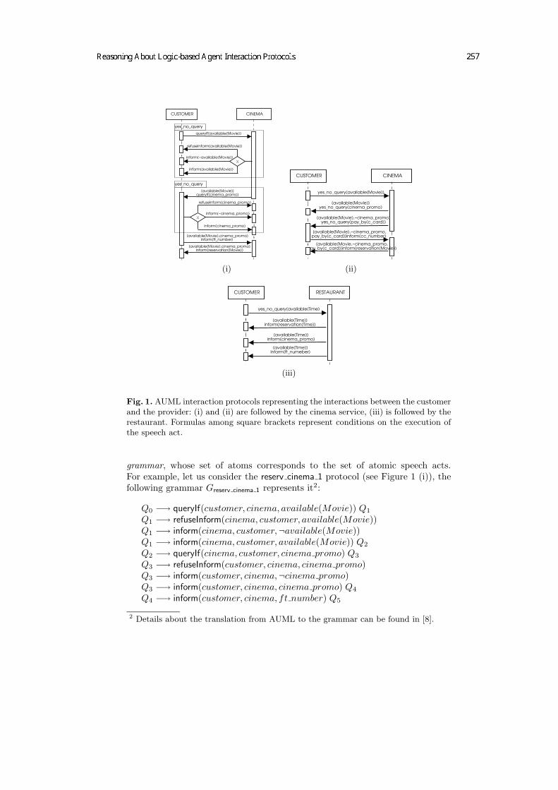
CINEMACUSTOMER

queryIf(available(Movie))

X

refuseInform(available(Movie))

inform(~available(Movie))

inform(available(Movie))

yes_no_query

[available(Movie)]queryIf(cinema_promo)

X

refuseInform(cinema_promo)

inform(~cinema_promo)

inform(cinema_promo)

[available(Movie),cinema_promo]inform(ft_number)

[available(Movie),cinema_promo]inform(reservation(Movie))

yes_no_query

CINEMACUSTOMER

yes_no_query(available(Movie))

[available(Movie)]yes_no_query(cinema_promo)

[available(Movie),~cinema_promo]yes_no_query(pay_by(c_card))

[available(Movie),~cinema_promo,pay_by(c_card)]inform(cc_number)

[available(Movie,~cinema_promo,pay_by(c_card)]inform(reservation(Movie))

(i) (ii)

RESTAURANTCUSTOMER

yes_no_query(available(Time)

[available(Time)]inform(reservation(Time))

[available(Time)]inform(cinema_promo)

[available(Time)]inform(ft_numeber)

(iii)

Fig. 1. AUML interaction protocols representing the interactions between the customerand the provider: (i) and (ii) are followed by the cinema service, (iii) is followed by therestaurant. Formulas among square brackets represent conditions on the execution ofthe speech act.

grammar, whose set of atoms corresponds to the set of atomic speech acts.For example, let us consider the reserv cinema 1 protocol (see Figure 1 (i)), thefollowing grammar Greserv cinema 1 represents it2:

Q0 −→ queryIf(customer, cinema, available(Movie)) Q1

Q1 −→ refuseInform(cinema, customer, available(Movie))Q1 −→ inform(cinema, customer,¬available(Movie))Q1 −→ inform(cinema, customer, available(Movie)) Q2

Q2 −→ queryIf(cinema, customer, cinema promo) Q3

Q3 −→ refuseInform(customer, cinema, cinema promo)Q3 −→ inform(customer, cinema,¬cinema promo)Q3 −→ inform(customer, cinema, cinema promo) Q4

Q4 −→ inform(customer, cinema, ft number) Q5

2 Details about the translation from AUML to the grammar can be found in [8].

Q5 −→ inform(cinema, customer, reservation(Movie))

By means of L(Greserv cinema 1) we denote the language generated by it. Intuitively,it represents all the legal conversations.

Now, we are in the position to give our first definition of conformance: theagent conformance.

Definition 1 (Agent conformance). Let D = (Π,CKitagi , S0) be a domain

description, pdylog ∈ CKitagi be an implementation of the interaction protocol

pAUML defined by means of an AUML sequence diagram. Moreover, let us define

the set Σ(S0) as σ|(Π,CKitagi , S0)`ps〈pdylog〉> w. a. σ. We say that the agent

described by means of D is conformant w.r.t. the sequence diagram pAUML if

and only if:

Σ(S0) ⊆ L(GpAUML) (1)

In other words, the agent conformance property holds if we can prove that everyconversation, that is an instance of the protocol implemented in our language (anexecution trace of pdylog), is a legal conversation according to the grammar thatrepresents the AUML sequence diagram pAUML; that is to say, that conversationis also generated by the grammar GpAUML

.The agent conformance depends on the initial state S0. Different initial states

can determine different possible conversations (execution traces). A notion ofagent conformance, that is independent from the initial state, can also be defined:

Definition 2 (Agent strong conformance). Let D = (Π,CKitagi , S0) be a

domain description, let pdylog ∈ CKitagi be an implementation of the interaction

protocol pAUML defined by means of an AUML sequence diagram. Moreover, let

us define the set Σ =⋃

S Σ(S), where S ranges over all possible initial states.

We say that the agent described by means of D is strongly conformant w.r.t. thesequence diagram pAUML if and only if:

Σ ⊆ L(GpAUML) (2)

In other words, the agent strong conformance property holds if we can prove thatevery conversation for every possible initial state is a legal conversation, i.e. it isalso generated by the grammar that represents the AUML sequence diagram. Itis easy to see that agent strong conformance (2) implies agent conformance (1).

Agent strong conformance, differently than agent conformance, does not de-pend on the initial state but it still depends on the set of speech acts definedin CKitagi . A stronger notion of conformance should require that a DyLOG im-plementation is conformant w.r.t. an AUML sequence diagram independently ofthe semantics of the speech acts. In other world, we would like to prove a sort of“structural” conformance of the implemented protocol w.r.t. the correspondingAUML sequence diagram. In order to do this, we define a formal grammar fromthe DyLOG implementation of a conversation protocol. In this process, the par-ticular form of axiom, namely inclusion axiom, used to define protocol clausesin a DyLOG implementation, comes to help us. Actually, such axioms have anatural interpretation as rewriting rules [2, 12].

Given a domain description (Π,CKitagi , S0) and an conversation protocolpdylog ∈ CKitagi = (ΠC , ΠCP , ΠSget), we define the grammar Gpdylog

= (T, V, P, S),where T is the set of all terms that define the set of speech acts in ΠC , V is theset of all the terms that define a conversation protocol or a get message actionin ΠCP or ΠSget. P is the set of production rules of the form p0 −→ p1p2 . . . pn

where 〈p0〉ϕ ⊃ 〈p1〉〈p2〉 . . . 〈pn〉ϕ is an axiom that defines either a conversationprotocol (that belongs to ΠCP) or a get message action (that belongs to ΠSget).Note that test actions 〈Fs?〉 are not reported in the production rules. Finally,the start symbol S is the symbol pdylog. Let us define L(Gpdylog

) as the languagegenerated by means of the grammar Gpdylog

. It is easy to see that L(Gpdylog) is

a context-free language since Gpdylogis a context-free grammar. Intuitively, the

language L(Gpdylog) represents all the possible sequences of speech acts (conver-

sations) allowed by the DyLOG protocol pdylog independently of the evolutionof the mental state of the agent.

Definition 3 (Protocol conformance). Let D = (Π,CKitagi , S0) be a domain

description, let pdylog ∈ CKitagi be an implementation of the interaction protocol

pAUML defined by means of an AUML sequence diagram. We say that pdylog is

conformant to the sequence diagram pAUML if and only if:

L(Gpdylog) ⊆ L(GpAUML

) (3)

It is possible to prove that protocol conformance (3) implies agent strong con-

formance (2).

In this case, it is straightforward to prove that for the customer viewreserv cinema 1C the protocol conformance holds w.r.t. protocol reserv cinema 1.It is worth noting the following property of the protocol conformance.

Proposition 1. Protocol conformance is decidable.

Proof. Equation (3) is equivalent to L(Gpdylog)∩L(GpAUML

) = ∅. Now, L(Gpdylog)

is a context-free language while L(GpAUML) is a regular language. Since the com-

plement of a regular language is still regular, L(GpAUML) is a regular language.

The intersection of a context-free language and a regular language is a context-free language. For context-free languages, the emptiness is decidable [15].

Proposition 1 tells us that an algorithm for verifying protocol conformanceexists. However, we also have a straightforward methodology for implementingprotocols in a way that conformance w.r.t. the AUML specification is respected.In fact, we can build our implementation starting from the grammar GpAUML

,and applying the inverse of the process that we described for passing from aDyLOG implementation to the grammar Gpdylog

. In this way we obtain a skele-ton of a DyLOG implementation of pAUML that is to be completed by addingthe desired ontology for the speech acts and customized with tests. Such animplementation trivially satisfies protocol conformance and, then, all the otherdegrees of conformance defined above.

4.2 Composition

One example in which it is useful to reason about protocol composition, is thesituation in which the same customer is supposed to interact with the restaurantand the cinema providers, one after the other. In fact, the developer must be surethat the customer, by interacting with the composition (by sequentialization)of the two protocols, will obtain what desired. In particular, suppose that thedeveloper wants to verify if the protocols that he/she defined allow the followinginteraction: it is possible to make a reservation at the restaurant and, then, atthe cinema, taking advantage of the promotion. Let us consider the query:

〈reserv rest 1C(customer, restaurant, dinner) ;reserv cinema 1C(customer, cinema,movie)〉

(Bcustomercinema promo ∧ Bcustomerreservation(dinner)∧Bcustomerreservation(movie) ∧ BcustomerBCft number)

that amounts to determine if it is possible to compose the interaction so to re-serve a table for dinner (Bcustomerreservation(dinner)) and to book a ticketfor the movie movie (Bcustomerreservation(movie)), exploiting a promotion(Bcustomercinema promo). The obtained free ticket is to be spent (Bcustomer

Bcinema ft number), i.e. customer believes that after the conversation the cho-sen cinema will know the number of the ticket given by the selected restaurant.

In the case in which the customer has neither a reservation for dinner nora reservation for the cinema or a free ticket, the query succeeds, returning thefollowing linear plan:

queryIf(customer, restaurant, available(dinner)) ;

inform(restaurant, customer, available(dinner)) ;

inform(restaurant, customer, reservation(dinner)) ;inform(restaurant, customer, cinema promo) ;inform(restaurant, customer, ft number) ;queryIf(customer, cinema, available(movie)) ;

inform(cinema, customer, available(movie)) ;

queryIf(cinema, customer, cinema promo) ;inform(customer, cinema, cinema promo) ;inform(customer, cinema, ft number) ;inform(cinema, customer, reservation(movie))

This means that there is first a conversation between customer and restaurant

and, then, a conversation between customer and cinema, that are instances ofthe respective conversation protocols, after which the desired condition holds.

Notice that the linear plan will actually lead to the desired goal given thatsome assumptions about the provider’s answers hold. In the above plan, assump-tions have been outlined with a box. For instance, that a seat at the cinema isfree. The difference with the other inform acts in the plan (from a provider to thecustomer) is that while for those the protocol does not offer any alternative, the

outlined ones correspond just to one of the possible answers foreseen by the pro-tocol. In the example they are answers foreseen by a yes no query protocol (seeFigure 1 (i) and [6]). The actual answer can be known only at execution time,however, thanks to the existence of the protocol, it is possible to understand theconditions that lead to success.

4.3 Selection

Another situation in which the developer may need support is to search into alibrary of available policies for an interaction protocol that describes a serviceof interest and that is suitable to the application that he/she is designing. Forinstance, the developer must design a protocol for a restaurant that allows tomake a reservation not necessarily using a credit card. In this case the developerwill first search the library of available protocols looking for those that satisfy thisrequest. This search cannot be accomplished only based on descriptive keywordsbut requires a form of reasoning on the way in which the interaction is carriedon. Suppose that search service is a procedure that allows one to search into alibrary for a protocol in a given category; then, the query would look like:

〈search service(restaurant, Protocol) ; Protocol(customer, service, time)〉(Bcustomer¬Bservicecc number ∧ Bcustomerreservation(time))

which means: look for a protocol that has one possible execution, after whichthe service provider does not know the customer’s credit card number, and areservation has been taken.

5 Conclusions and related work

In this paper we have proposed a logic-based approach to agent interaction proto-col specification and we have shown the advantages of using reasoning techniquesbased on such a logical formalization, especially in the context of agent-orientedsoftware engineering (AOSE). We used as agent language DyLOG, a high-levellogic programming language for modeling and programming rational agents,based on a modal theory of actions and mental attitudes, that allows to includein the agent specification a set of interaction protocols. The DyLOG languageallows reasoning about the effects of engaging specific conversations. By doingso, an agent can plan a conversation for achieving a particular goal, that re-spects the protocol, while the system designer can exploit the same reasoningtechniques to select a protocol from a library or to verify if the composition ofa set of given protocols respects some desired constraint.

Moreover, we have shown that our logical representation of protocols allowsus to deal with the matter of checking the agent conformance w.r.t. a protocolrepresented as a AUML interaction diagram. This is a crucial problem to face inan AOSE perspective and it can be considered as a part of the process of engi-neering interaction protocols sketched in [16]. Indeed, supposing to have both an

AUML sequence diagram, which formally specifies a protocol, and an implemen-tation of the same protocol in DyLOG, a key problem to solve is checking theconformance of the implementation to the diagram. In fact, when protocols areimplemented in DyLOG they become part of the agent communication policies,which are usually determined by the agent mental state. What we check is ifthis strategy is conformant to the AUML protocol, at least in the sense that theagent never performs any illegal dialogue move. In other words we prove a sortof “structural” conformance of the implemented protocol w.r.t the specification.

The problem of checking the agent conformance to a protocol in a logicalframework has been faced also in [11]. In a broad sense our notion of confor-mance bears along some similarities with the notion of agent weak conformance,introduced in this work. In [11] agent communication strategies and protocolspecification are both represented by means of sets of if-then rules in a logic-based language, which relies on abductive logic programming. A notion of weakconformance is introduced, which allows to check if the possible moves that anagent can make, according to a given communication strategy, are legal w.r.t.the protocol specification. The conformance test is done by abstracting from (i.e.disregarding) any condition related to the agent private knowledge, which is notconsidered as relevant in order to decide weak conformance, although it could,actually, prevent an agent from performing a particular move.

Our framework allows us to give a finer notion of conformance, for which wecan distinguish different degrees of abstraction with respect to the agent privatemental state. It allows us to define in an elegant manner which parts of a protocolimplementation must fit the protocol specification and to describe in a modularway how the protocol implementation can be enriched with respect to the pro-tocol specification, without compromising the conformance. Such an enrichmentis important when using logic agents, that support sophisticated forms of rea-soning. Indeed, the ability of reasoning about the properties of the interactionsthat occur among agents before they actually occur, may by applied to supporta MAS developer during the design phase. We have recently begun to study [4]the methodological and physical integration of DyLOG into the DCaseLP [1, 18]MAS prototyping environment following the what already done for integratingtuProlog [14]. The aim of this work is to enrich the DCaseLP framework withthe ability of reasoning about AUML interaction protocols thanks to a transla-tion from AUML to DyLOG. In this context it will be extremely useful to haveformal methods for proving conformance properties.

Acknowledgement

This research is partially supported by MIUR Cofin 2003 “Logic-based develop-ment and verification of multi-agent systems” national project.

References

1. E. Astesiano, M. Martelli, V. Mascardi, and G. Reggio. From Requirement Spec-ification to Prototype Execution: a Combination of a Multiview Use-Case Driven

Method and Agent-Oriented Techniques. In J. Debenham and K. Zhang, edi-tors, Proceedings of the 15th International Conference on Software Engineeringand Knowledge Engineering (SEKE’03), pages 578–585. The Knowledge SystemInstitute, 2003.

2. M. Baldoni. Normal Multimodal Logics: Automatic Deduction and Logic Program-ming Extension. PhD thesis, Dipartimento di Informatica, Universita degli Studidi Torino, Italy, 1998. Available at http://www.di.unito.it/~baldoni/.

3. M. Baldoni. Normal Multimodal Logics with Interaction Axioms. In D. Basin,M. D’Agostino, D. M. Gabbay, S. Matthews, and L. Vigano, editors, Labelled De-duction, volume 17 of Applied Logic Series, pages 33–53. Applied Logic Series,Kluwer Academic Publisher, 2000.

4. M. Baldoni, C. Baroglio, I. Gungui, A. Martelli, M. Martelli, V. Mascardi, V. Patti,and C. Schifanella. Reasoning about agents’ interaction protocols inside dcaselp. InJ. Leite, A. Omicini, P. Torroni, and P. Yolum, editors, Proc. of the InternationalWorkshop on Declarative Language and Technologies, DALT’04, New York, July2004. To appear.

5. M. Baldoni, C. Baroglio, A. Martelli, and V. Patti. Reasoning about ConversationProtocols in a Logic-based Agent Language. In A. Cappelli and F. Turini, editors,AI*IA 2003: Advances in Artificial Intelligence, 8th Congress of the Italian Asso-ciation for Artificial Intelligence, volume 2829 of LNAI, pages 300–311. Springer,September 2003.

6. M. Baldoni, C. Baroglio, A. Martelli, and V. Patti. Reasoning about self and others:communicating agents in a modal action logic. In C. Blundo and C. Laneve, editors,Theoretical Computer Science, 8th Italian Conference, ICTCS’2003, volume 2841of LNCS, pages 228–241, Bertinoro, Italy, October 2003. Springer.

7. M. Baldoni, C. Baroglio, A. Martelli, and V. Patti. Reasoning about interactionprotocols for web service composition. In M. Bravetti and G. Zavattaro, editors,Proc. of 1st Int. Workshop on Web Services and Formal Methods, WS-FM 2004,Electronic Notes in Theoretical Computer Science. Elsevier Science Direct, 2004.

8. M. Baldoni, C. Baroglio, A. Martelli, V. Patti, and C. Schifanella. Verifying pro-tocol conformance for logic-based communicating agents. Submitted, 2004.

9. M. Baldoni, L. Giordano, and A. Martelli. A Tableau Calculus for MultimodalLogics and Some (Un)Decidability Results. In H. de Swart, editor, Proc. ofTABLEAUX’98, volume 1397 of LNAI, pages 44–59. Springer-Verlag, 1998.

10. M. Baldoni, L. Giordano, A. Martelli, and V. Patti. Programming Rational Agentsin a Modal Action Logic. Annals of Mathematics and Artificial Intelligence, Specialissue on Logic-Based Agent Implementation, 41(2-4), 2004. To appear.

11. Ulrich Endriss, Nicolas Maudet, Fariba Sadri, and Francesca Toni. Logic-basedagent communication protocols. In F. Dignum, editor, Advances in agent commu-nication languages, volume 2922 of Lecture Notes in Artificial Intelligence (LNAI).Springer-Verlag, 2004. To appear.

12. L. Farinas del Cerro and M. Penttonen. Grammar Logics. Logique et Analyse,121-122:123–134, 1988.

13. F. Guerin and J. Pitt. Verification and Compliance Testing. In H.P. Huget,editor, Communication in Multiagent Systems, volume 2650 of LNAI, pages 98–112. Springer, 2003.

14. I. Gungui and V. Mascardi. Integrating tuProlog into DCaseLP to engineer het-erogeneous agent systems. Parma, Italy, June 2004. In this volume.

15. J. E. Hopcroft and J. D. Ullman. Introduction to automata theory, languages, andcomputation. Addison-Wesley Publishing Company, 1979.

16. M. P. Huget and J.L. Koning. Interaction Protocol Engineering. In H.P. Huget,editor, Communication in Multiagent Systems, volume 2650 of LNAI, pages 179–193. Springer, 2003.

17. S. Breuckner J. Odell, H. Van Dyke Parunak and M. Fleischer. Temporal aspects ofdynamic role assignment. In J. Odell P. Giorgini, J. Muller, editor, Agent-OrientedSoftware Engineering (AOSE) IV, volume (forthcoming) of LNCS, Berlin, 2004.Springer.

18. M. Martelli and V. Mascardi. From UML diagrams to Jess rules: Integrating OOand rule-based languages to specify, implement and execute agents. In F. Bucca-furri, editor, Proceedings of the 8th APPIA-GULP-PRODE Joint Conference onDeclarative Programming (AGP’03), pages 275–286, 2003.

19. M. Martelli, V. Mascardi, and F. Zini. Caselp: a prototyping en-vironment for heterogeneous multi-agent systems. Available athttp://www.disi.unige.it/person/MascardiV/Download/aamas-journal-MMZ04.ps.gz.

20. V. Mascardi, M. Martelli, and L. Sterling. Logic-Based Specification Languages forIntelligent Software Agents. Theory and Practice of Logic Programming Journal,2004. to appear.

21. J. Odell, H. V. D. Parunak, and B. Bauer. Extending UML for agents. In Pro-ceedings of the Agent-Oriented Information System Workshop at the 17th NationalConference on Artificial Intelligence. 2000.

Contracts in Multiagent Systems:the Legal Institution Perspective

Guido Boella1 and Leendert van der Torre2

1Dipartimento di Informatica - Universita di Torino - Italy, guido@di.unito.it2CWI - Amsterdam - The Netherlands, torre@cwi.nl

Abstract. In this paper we address the problem of how the autonomy of agents inan organization can be enhanced by means of contracts. Contracts are modelled aslegal institutions: systems of legal rules which allow to change the regulative andconstitutive rules of an organization. The methodology we use is to attribute toorganizations mental attitudes, beliefs, desires and goals, and to take into accounttheir behavior by using recursive modelling.

1 Introduction

One of the main challenges in multi-agent societies is the coordination of the au-tonomous agents. Coordination can be achieved finding a trade off between a bottom-upview and a top-down view of the problem. In the former, the MAS is an aggregationof autonomous agents interacting with each other, where their emergent behavior is notnecessarily the desired one. In the latter, the system’s objectives are achieved withoutrequiring specific agent’s internal design, by means of organizational design togetherwith roles and norms as incentives for cooperation.

As Dignumet al. [12] note, however, the interaction structure of the organizationshould be not be completely fixed in advance. The autonomy of the agents should bepreserved even if within limits. For this reason, some approaches like [10, 12, 19] in-troduce the possibility for agents to stipulate contracts. A contract can be defined as astatement of intent that regulates behavior among organizations and individuals. Con-tracts have been proposed as means to make explicit the way agents can change theinteraction with and within the society: they create obligations, permissions and newpossibilities of interactions. From a contractual perspective, organizations can be seenas the possible sets of agreements for satisfying the diverse interests of self interestedindividuals [10].

Social order, thus, emerges from the negotiation of contracts about the rights andduties of participants, rather than being given in advance. But the organization itselfspecifies the possible contracts and enforces the obligations created by them as theywere issued by the organization itself. As Ruiter [20] shows, however, from the legalpoint of view, legal effects of actions of the members of a legal system (as an organiza-tion is) are a difficult problem. Contracts do not concern only the regulative aspects of alegislation (i.e., the rules of behavior specified in obligations), or the constitutive part ofit (i.e., the rules introducing institutional facts such bidding in an auction). Rather, con-tracts arelegal institutions: “systems of [regulative and constitutive] rules that provide

frameworks for social action within larger rule-governed settings” [20]; in our case thelarger setting is represented by organizations.

This systemic view of legal institutions emerged only recently in legal studies [20],since legal positivism [15] mainly focused on the regulative aspects of law and its jus-tification. For this reason is necessary to address the problem of contracts being awareof the peculiarities of legal institutions.

The research question of this paper is: how can be legal institutions, like contracts,be formalized? and, as subquestions, how can agents modify the behavior of the orga-nization via contracts? Which games can agents play when they are allowed to makecontracts?

As methodology we use the agent metaphor: we attribute to organizations mentalattitudes, beliefs, desires and goals, and we take into account their behavior by usingrecursive modelling [13]. We apply to organizations the methodology we adopted forsocial entities like groups, virtual communities [4] and normative multiagent systems[3, 7, 6].

In the next section we discuss constitutive rules and how legal institutions are cre-ated. In Section 3 we discuss the conceptual model, with the definition of obligationsand contracts. In Section 4 we present the games which can be played with contracts,together with a detailed example. Related work and summary close the paper.

2 Legal institutions

Normative multiagent systems, like organizations, are “sets of agents [...] whose inter-actions can be regarded as norm-governed; the norms prescribe how the agents ideallyshould and should not behave. [...] Importantly, the norms allow for the possibility thatactual behavior may at times deviate from the ideal, i.e., that violations of obligations,or of agents’ rights, may occur” (Jones and Carmo [16]).

In [3] we formalize the relation between multiagent systems and normative systemsby attributing mental states to agents as well as to normative systems, as proposed byBoella and Lesmo [2]. The agent metaphor may be seen as an instance of Dennett’sintentional stance[11] and is inspired by the interpretation of normativemultiagentsystems as dynamic social orders. According to Castelfranchi [8], a social order is apattern of interactions among interfering agents “such that it allows the satisfaction ofthe interests of some agent”. These interests can be a shared goal, a value that is goodfor everybody or for most of the members. But the agents attribute to the normativesystem, besides goals, also the ability to autonomously enforce the conformity of theagents to the norms by means of sanctions. In this approach the obligations of the agentscan be formalized as desires or goals of the normative agent. This representation maybe paraphrased as “Your wish is my command” because the desires or wishes of thenormative agent are the obligations or commands of the other agents.

Most formalizations of normative systems, however, including [3], identify normswith obligations, prohibitions and permissions. This is not sufficient in complex norma-tive multiagent systems for the following three reasons. First of all, these norms, calledregulative norms, specify all the conditions when they are applicable. It would be moreeconomic that regulative norms could factor out particular cases and could refer to

more abstract concepts only. Hence, the normative system should include mechanismsto introduce new legal categories of abstract entities for classifying possible states ofaffairs. Second, the dynamics of the social order is due to the fact that the normativesystem evolves over time by introducing new norms and abrogating outdated ones. Sothe normative system itself must specify how it can be changed by introducing newregulative norms, new legal categories and by whom the changes can be done. Third,the dynamics of a normative system includes the possibility that not only new normsare introduced by the legislators, but also that ordinary agents create new obligationsand permissions concerning specific agents. This feature is fundamental to preserve theautonomy of agents inside an organization. In particular, it allows modelling contractswhich introduce new normative relations among agents, like the duty to pay a fee for aservice.

We therefore introduce a formal framework for the construction of normative multi-agent systems, based on Searle’s notion of the construction of social reality. Searle [21]argues that there is a distinction between two types of rules, a distinction which alsoholds for formal rules like those composing normative systems:

Some rules regulate antecedently existing forms of behaviour. For example,the rules of polite table behaviour regulate eating, but eating exists indepen-dently of these rules. Some rules, on the other hand, do not merely regulate anantecedently existing activity called playing chess; they, as it were, create thepossibility of or define that activity. The activity of playing chess is constitutedby action in accordance with these rules. The institutions of marriage, money,and promising are like the institutions of baseball and chess in that they aresystems of such constitutive rules or conventions ([21], p. 131).

For Searle, institutional facts like marriage, money and private property emergefrom an independent ontology of “brute” physical facts through constitutive rules of theform “such and such an X counts as Y in context C” where X is any object satisfyingcertain conditions and Y is a label that qualifies X as being something of an entirelynew sort. E.g., “X counts as a presiding official in a wedding ceremony”, “this bit ofpaper counts as a five euro bill” and “this piece of land counts as somebody’s privateproperty”.

Like we formalize obligations in terms of desires and goals, in the next section, weformalize the constitutive rules as belief rules of the normative agent. E.g., consider asociety which believes that a field fenced by an agent counts as the fact that the fieldis property of that agent. The fence is a physical “brute” fact, while being a property isan institutional fact attributed to the beliefs of the normative system. Regulative normswhich forbid trespassing refer to the abstract concept of property rather than to fencedfields. As the system evolves, new cases are added to the notion of property, withoutchanging the regulative norms about property. E.g., if a field is inherited, then it isproperty of the heir.

Searle’s analysis of constitutive rules has focused mainly on the attribution of anew functional status to entities, as in the examples above: marriages, money, property.Searle’s idea is that constitutive rules “create the possibility or define that activity”. Webelieve, however, that the role of constitutive rules is not limited to the creation of an

activity and the construction of new abstract legal categories. Constitutive norms specifyboth the creation of legal categories and the evolution of the system: the normativesystem itself specifies by means of constitutive rules (included in its belief rules) howits beliefs, desires and goals can be changed, who can change them, and the limits ofthe possible changes. In this way, complex normative systems achieve a legal regimethat includes rules conferring legal powers on certain participants: an agent is turnedon a “private legislator” (Hart, [15]): “he is made competent to determine the course oflaw within the sphere of his contracts, trusts, wills and other structures [...] which he isenabled to build”. Agents become able to design “relatively independentinstitutionallegal orderswithin the comprehensive legal orders” (Ruiter [20]).

The regime of a legal institution can be defined as the set of legal consequencesthat flow from the existence of the institution. However, the meaning of “legal conse-quences” differs from what is normally understood by the term. Usually, since obliga-tions have a conditional nature, when the conditions of an obligation are satisfied, as alegal consequence the addressee of the obligation is categorically obliged to fulfill it.Legal institutions, like contracts, marriages and properties, refer to a different kind oflegal consequences; e.g., the legal rule “in a marriage parents have the reciprocal obli-gation to take care of and support their children” is not a conditional rule: it expressesthe fact that when a legal institution of marriage comes into existence (say betweenAmy and Bob) only then the obligation that the spouses (Amy and Bob) take care andsupport their children is created. The same happens with the legal institution of con-tracts: when a contract comes into existence it creates obligations for the parties, i.e.,new regulative rules which the normative system considers as its own. E.g., the ItalianCivil Code art. 1173 (sources of obligations) specifies that obligations are created bycontracts and art. 1372 (efficacy of contracts) that a contract has the strength of law (acontract is an agreement among two or more parties to regulate a juridical relationshipabout valuablesexart. 1321).

Moreover, contracts as legal institutions bring with them not only new regulativerules, but also constitutive ones which create new institutional facts and also new obli-gations; in this way, it is possible to specify in a contract new procedures for the inter-action between parties, for specifying the evolution of the contract and how new obliga-tions are created later. As Dignumet al. [12] notice, a contract specifies the events thatalter the status of the contract. It is necessary to specify an interaction structure whichindicates the possibility of an agent and the consequences of its choices; the contractmust specify how to proceed if a norm is violated and what the violator is expected todo; e.g., if some payment deadline is not respected, the agent is obliged to pay a doublefee. Since we model contracts as legal institutions, we are now aware that this rule isnot a conditional obligation: it is an obligation created by some event specified in thecontract, in the same way as the contract itself can create obligations. This is possiblebecause we consider a contract as a legal institution, i.e., a normative system insidethe main normative system: as a normative system it specifies who has the power tointroduce obligations.

3 The conceptual model

In order to provide a formalization of contracts as legal institutions in organizations wefirst delineate the conceptual model we adopt.

First of all, the structural concepts and their relations. We have to describe the dif-ferent aspects of the world and the relationships among them. We therefore introducea set of propositional variablesX and we extend it to consider also negative states ofaffairs:L(X) = X ∪ ¬x | x ∈ X. Moreover, forx ∈ X we write∼ x for ¬x and∼ (¬x) for x. The relations between the propositional variables are given by means ofconditional rules written asR(X) = 2L(X) × L(X): the set of pairs of a set of literalsbuilt from X and a literal built fromX, written asl1 ∧ . . . ∧ ln → l, and, whenn = 0,> → l. The rules will be used to represent the relations among propositional variablesexisting in beliefs, desires and goal of the agents.

Then there are the different sorts of agentsA we consider. Besides real agentsRA(either human or artificial) we consider as agents in the model also socially constructedagents like groups, normative systems and organizationsSA. These latter agents do notexist in the usual sense of the term. Rather, they exist only as they are attributed mentalattitudes by other agents (either real or not). By mental attitudes we mean beliefsB,desiresD and goalsG.

Coming to the relations existing between these structural concepts, mental attitudes,even if they do not coincide with, are represented by rules:MD : B∪D∪G → R(X).When there is no risk of confusion we will abuse the notation by identifying rules andmental states. To resolve conflicts among motivations we introduce a priority relation bymeans of≥: A → 2M ×2M a function from agents to a transitive and reflexive relationon the powerset of the motivations containing at least the subset relation. We write≥a for ≥ (a). Moreover, different mental attitudes are attributed to all the differentsorts of agents by the agent description relationAD : A → 2B∪D∪G∪A. We writeBa = AD(a) ∩B, Aa = AD(a) ∩A for a ∈ A, etc.

Also agents are in the target of theAD relation for the following reason: groups,normative systems, and organizations agents exist only as profiles attributed by otheragents. So groups, normative systems and organizations exist only as they are describedas agents by other agents, according to the agent description relation. TheAD relationinduces an exists-in-profile relation specifying that an agentb ∈ SA exists only as someother agents attribute to it mental attitudes:a | b ∈ Aa.

Finally, the different sorts of agents are disjoint and are all subsets of the set ofagentsA: RA ∪ SA ⊆ A.

We introduce now concepts concerning informational aspects. First of all, the setof variables whose truth value is determined by an agent (decision variables) [17] aredistinguished from those which are notP (the parameters).

Besides, we need to represent also the so called “institutional facts”I. They arestates of affairs which exist only inside normative systems and organizations. As dis-cussed in the previous section, Searle [22] suggests, money, properties, marriages existonly as part of social reality; since we model social reality by means of the attributionof mental attitudes to social entities, institutional facts are just in the beliefs of theseagents. Similarly, we need to represent that social entities like normative systems andorganizations are able to change themselves. The actions determining the changes are

called creation actionsC. Finally, we introduce contractsCT : they are agreements be-tween agents in normative systems or organizations which have legal consequences;they are defined in Section 3.2.

As concerns the relations among these concepts, we have that parametersP area subset of the propositional variablesX. The complement ofX andP represents thedecision variables controlled by the different agents. Hence we have to associate to eachagent a subset ofX \ P by extending again the agent description relationAD : A →2B∪D∪G∪A∪(X\P ).

Moreover, the institutional factsI are a subset of the parametersP : I ⊆ P . And thecreation actionsC are a subset of the institutional factsC ⊆ I: they do not exist outsidethe mind of agents and they have effects on the mental attitudes of agents only as far asthe agents believe they have.

Since social entities depend on the attribution of mental attitudes, we represent theirmodification by means of the modification of their mental attitudes expressed as rules.So the creation action relationCR : b, d, g×A×R(X) → C is a mapping from rules(for beliefs, desires and goals) to propositional variables, whereCR(b, a, r) stands forthe creation ofm ∈ Ba, CR(d, a, r) stands for the creation ofm ∈ Da, andCR(g, a, r)stands for the creation ofm ∈ Ga, such that the mental attitude is described by the ruler ∈ R(X): r = MD(m). For space reasons, in this paper we consider only the creationof new rules and not their deletion from the mental attitudes of an agent.

Since institutional factsI and the creation actionsC exist only in the beliefs of anormative system or an organization, we need a way to express how these beliefs can bemade true. As we discussed in the previous section, the relations among propositionalvariables are expressed as rules. In this case we have rules concerning beliefs about in-stitutional facts: they are called constitutive rules and represent the “counts as” relationsintroduced by Searle [22] (see previous section). We thus identify the subsetCN of thebelief rules which express the relation between propositional variables and institutionalfacts: rulesC∪x → y ∈ R(X) expressing the fact that a literalx ∈ L(X) in contextC ⊆ Lit(X) counts as the institutional facty ∈ L(I).

Finally, we have to model the effect of the creation actions on the mental attitudesof agents. For this reason we introduce an update relationUP from creation actions andmental attitudes to set of rules representing the new mental attitudesUP : B, D, G×C → 2B,D,G. Since a decision of an agent can make true some creation actions, theconsequences of these actions must be considered in the subsequent reasoning of theagent. The update function can be used to define the history of the multiagent systemrepresenting its evolution. Note that in this paper we do not consider the problem ofthe belief (and goal) revision. While this problem is sometimes addressed when dealingwith normative systems, we consider here only the problem of introducing we rules andnot of deciding which rules are necessary to get a certain revision.

We can now define a multiagent system asMAS = 〈RA, SA,X, P,B, D,G, C, AD,MD,≥, I, CT 〉.

We need to introduce normative multiagent systems to model organizations whichare able to issue and enforce obligations: let the normative agento ∈ SA be an agentrepresenting the organization. Let the normsn1, . . . , nm = N be a set. Let the normdescriptionV : N → Xo ∪ P be a complete function from the norms to the decision

variables of the normative agent together with the parameters: we writeV (n, a) for thedecision variable which represents that there is a violation of normn by agenta ∈ A.With these elements we define sanction based obligations in the next section. The tu-ple 〈RA, SA,X, P,B,D, G,C, AD,MD,≥, I, CT,o, N, V 〉 is a normative multia-gent systemNMAS.

As concerns the behavior of agents, in Section 4, we introduce the games that canbe played between two agentsa ando. Before games, we have to introduce two furthernotions: consequences of beliefs and decisions of agents.

To incorporate the consequences of belief rules, we introduce a simple logic of rulescalledout: it takes the transitive closure of a set of rules, called reusable input/outputlogic in [18]; out(E,S) be the closure ofS ⊆ L(X) under the rulesE:

– out0(E,S) = S

– outi+1(E, S) = outi(E, S) ∪ l | L → l ∈ E,L ⊆ outi(E, S)) for i ≥ 0

– out(E, S) = ∪∞0 (E, S)

We can now introduce decisions of agents; they must be consistent with the con-sequences of beliefs according to the two agentsa (out(Ba, δ)) ando (out(Bo, δo ∪out(Bo, δa))). The set of decisions∆ is the set of subsetsδ = δa ∪ δo ⊆ L(X) suchthat their closures under the beliefsout(Ba, δ) andout(Bo, δo ∪ out(Bo, δa)) do notcontain a variable and its negation.

3.1 Obligations

Since contracts affect the obligations of an agent, we must first summarize their defini-tion given in [3]. Obligations are defined in terms of goals of the addressee of the norma and of the organizationo. The definition of obligation contains several clauses. Thefirst one is the central clause of our definition and defines obligations of agents as goalsof the normative agent, following the ‘Your wish is my command’ strategy [3]. The firstclause says that the obligation is implied by the desires of agento, implied by the goalsof agento.

The second and third clauses can be read as “the absence ofp is considered as aviolation”. The association of obligations with violations is inspired to Anderson [1]’sreduction of deontic logic to alethic logic. The third clause says that the agent desiresthat there are no violations.

The fourth and fifth clauses relate violations to sanctions. The fourth clause assumesthat agento is motivated not to count behavior as a violation and apply sanctions as longas their is no violation; otherwise the norm would have no effect. Finally, for the samereason, we assume in the last clause that the agent does not like the sanction.

Definition 1 (Obligation). LetNMAS = 〈RA, SA, X, P,B, D,G, C, AD,MD,≥, I, CT,o, N, V 〉 be a normative multiagent system.

Agenta ∈ A is obliged to decide to dox ∈ L(Xa∪P ) with sanctions ∈ L(Xo∪P )if Y ⊆ L(Xa ∪ P ) in NMAS, written asNMAS |= Oao(x, s|Y ), if and only if:

1. Y → x ∈ Do ∩Go: if agento believesY then it desires and has as a goal thatx.2. Y ∪∼x → V (∼x,a) ∈ Do ∩Go: if agento believesY and ∼x, then it has the

goal and the desireV (∼x,a): to recognize it as a violation by agenta.3. > → ¬V (∼x,a) ∈ Do: agento desires that there are no violations.4. Y ∪ V (∼x,a) → s ∈ Do ∩ Go: if agento believesY and decidesV (∼x,a),

then it desires and has as a goal that it sanctions agenta.5. Y → ∼s ∈ Do: if agent o believesY , then it desires not to sanction∼s . This

desire of the normative system expresses that it only sanctions in case of violation.6. Y → ∼s ∈ Da: if agenta believesY , then it desires∼s, which expresses that it

does not like to be sanctioned.

Permissions and prohibitions can be defined in terms of motivational attitudes, too[4].

As discussed in [3], sanctions or rewards are not the only possible motivations tostick to obligations, but they are necessary to cope for the worst cases.

3.2 Contracts

Contracts are part of the beliefs attributed to the organizationo: this fact makes it pos-sible that they change the beliefs of the organization according to what specified by theorganization itself.

A contractct ∈ CT is created (a fact represented by the institutional factc ∈ I) onlyif the organization believes that some other fact has as a consequence thatc is true. Moreprecisely, if there is some fact which counts asc for the organizationo. This fact canbe a brute fact in the world or another institutional fact. E.g., since contracts are createdby agreements, the contractc is created by the signatures of two agents, two decisionvariablese andf : a constitutive norm in the belief rules of agento (e ∧ f → c ∈ Bo).One reason why the creation of the contractc is introduced as an intermediary betweenthe agreement and its legal effects is that, as many other institutional facts, it allowsdecoupling the conditions of the creation of the institutional facts from its legal effects.In this way, e.g., it is possible to specify new ways of creating the contract (for instanceusing an electronic signature) maintaining the same rules specifying its legal effects.

The effect a contract achieves is to modify the mental attitudes of the normativesystem. Usually, it adds more than one rule to the beliefsBo, the desiresDo, or thegoalsGo by making true some creation actions inC. Again, the creation actions areinstitutional facts: they are made true only if the organizationo believes that they aremade true by the creation of the contract: e.g.,c → t ∈ Bo, is another constitutive rule,read asc ∈ I counts as the creation actiont ∈ C. Since a contract counts as severalcreation actionst ∈ C, the conclusion is thatc works as an abstraction: rather thanconnecting the signatures of the agents with the creation actions, the contract unifies allthe legal effects.

Finally, we consider which mental attitudes are changed. A contract modifies themental attitudes of the normative system: since both regulative rules like obligationsand constitutive ones like those composing contracts are themselves defined in terms ofmental attitudes of the normative system, a contract can have legal effects.

By making true some creation actions, a contract is able to create regulative normsas the obligations of an agenta to pay (pay ∈ Xa) in case the requested good has beenshipped to him;Oao(pay, s | shipped) is defined by the normative goal and desire thatshipped goods are payed:shipped → pay ∈ Do ∩Go; the goal and desire to considerthe lack of payment for shipped goods as a violation:shipped∧¬pay → V (¬pay,a) ∈Do ∩ Go. And finally, the goal and desire to sanction violations:V (¬pay,a) → s ∈Do ∩ Go; avoiding the sanction> → ¬s is a desire of agentsa ando, thus, it is aprecondition of the obligation [5].

The creation of the contract achieves these effects on the mental attitudes of theorganizationo since it counts as a series of creation actions: that the goals and desiresdefining the obligation are added. Since the counts as relation is described by constitu-tive rules in the beliefs of agento we have (as concerns goals):

c → CR(g,o, shipped → pay),

c → CR(g,o, shipped ∧ ¬pay → V (¬pay,a)),

c → CR(g,o, V (¬pay,a) → s)

⊆ Bo.

Also constitutive rules can be created by contracts: they are defined by belief rulesof the normative systemo, so they are created by a creation actionCR(b,o, t) ∈ C.

First of all, the contract may specify some institutional fact which should be usedin the interaction. E.g., the shipment of the exchanged good is an institutional factshipped ∈ I; the fact that the good has been shipped is not a brute fact of the world(the buyer cannot check it), rather it is a fact which holds if there is some docu-ment like the so called bill of lading (bill ∈ P ) issued by a third party [14]:bill →shipped is the rulet added to the beliefs of the organizationo by the creation actionCR(b,o, t) ∈ C; the creation action is a consequence of the contractc: the constitutiverule c → CR(b,o, bill → shipped) ∈ Bo creates another constitutive rule.

Second, constitutive rules created by contracts will introduce new obligations andnew constitutive rules. In this way a contract can specify how new obligations may ariseduring the interaction of the parties. We return on [12]’s example: if an agent does notpay the fee for a shipped good, it is obliged to pay a double sum of money (pay2):Oao(pay2, s′ | shipped ∧ ¬pay). This obligation is not a preexisting conditional obli-gation: it is created as a legal consequence of an event, the sanctions for not havingpayed the fee. The sanctions, in this case, rather than being a direct punishment foragenta, counts as the action of creating a second obligation.Note that this obligation

does not exist until the normative system recognizes a violation and applies the sanc-tion s. This part of the contract is thus represented by the constitutive rules which createfurther constitutive rules about goals (wheres′ ∈ Xo is a sanction both feared by agenta and not desired by agento): e.g.,

c → CR(b,o, s → CR(g,o, shipped ∧ ¬pay → pay2)),c → CR(b,o, s → CR(g,o,¬pay2 → V (¬pay2,a)))

⊆ Bo

In summary, a contract is defined as:

Definition 2 (Contract). A contractct ∈ CT is a triple:

1. An institutional factc ∈ I representing that the contractct ∈ CT has been created.2. A constitutive rule which makes true the institutional factc: Y → c ∈ Bo where

Y ⊆ L(X)3. A set of constitutive rules having as antecedent the creationc of the contractct and

as consequent creation actions modifying the mental attitudes of the organizationo: c → CR(E,o, r) ∈ Bo whereE = b, d, g.

4 Games

The advantage of the attribution of mental attitudes to organizations is that standardtechniques developed in decision and game theory can be applied to reasoning on con-tracts. Here we consider a simple form of games of two stages only where an agentatakes the normative agento into account by playing games with it.

When agenta takes its decisionδa it has to minimize its unfulfilled motivationalattitudes. But when it considers these attitudes, it must not only consider its decisionδa and the consequences of this decision; it must consider also the decisionδo of theorganizationo and its consequences, for example that it is sanctioned by agento. Soagenta recursively considers which decision agento will take depending on its differentdecisionsδa. Note that here we assume thato is aware of agenta’s decision: hence,agento takes its decision considering the legal effects of agenta’s decision on its beliefsand motivations using the update functionUP and the creation actions made true bythe decisionδa.

Given a decisionδa, a decisionδo is optimal for agento if it minimizes the unful-filled motivational attitudes inDo andGo according to the≥o relation. The decisionof agenta is more complex: for each decisionδa it must consider which is the optimaldecisionδo for agento.

Definition 3 (Recursive modelling).Let:

– the unfulfilled motivations of decisionδ according to agenta ∈ A be the set ofmotivations whose body is part of the closure of the decision under the belief rulesbut whose head is not.

U(δ,a) = m ∈ M | MD(m) = l1∧. . .∧ln → l, l1, . . . , ln ⊆ out(Ba, δ) andl 6∈out(Ba, δ).

out(E, Bo, ¬y ∪ out(E, Br, x))

XXXXXz

»»»»»:XXXXXz

»»»»»:XXXXXz

out(E, Br, x)

©©©©©*x

HHHHHj¬x

»»»»»:XXXXXz

6............

?

............HHHHHj

©©©©©*

y

¬y

y, p

¬y, p

y

¬y

y

¬y

δo U(δa ∪ δo,a)

y

¬y

y, p

¬y, p

out(E, Ba, y ∪ ¬x)

out(E, Ba, ¬y ∪ ¬x)

out(E, Bo, y ∪ out(E, Br, ¬x))

out(E, Bo, ¬y ∪ out(E, Br, ¬x))

y

¬y

y

¬y

out(E, Ba, ¬y ∪ x)

out(E, Ba, y ∪ x)

out(E, Bo, y ∪ out(E, Br, x))

x → ¬y

x → ¬y

> → ¬x,¬x → ¬y

> → ¬x

> → ¬x,¬x → ¬y

> → ¬x

δa

x, p

x

x, p

out(E, Br, ¬x)

out(E, Ba, x)

out(E, Ba, ¬x) ¬x

x

¬x

»»»»»:

Fig. 1. The game between agenta and agento.

– the unfulfilled motivations of decisionδ according to agento be the set of motiva-tions whose body is part of the closure of the decision under the belief rules andwhose head is not, but considering the consequences of agenta’s decision on agento’s beliefs and motivations. We writeO = out(Bo, δa) ∩ C for the set of creationactions which follow fromδa:

U(δ,o) = m ∈ UP (Do ∪Go, O) | MD(m) = l1 ∧ . . .∧ ln → l, l1, . . . , ln ⊆out(UP (Bo, O), δo ∪ out(Bo, δa)) andl 6∈ out(UP (Bo, O), δo ∪ out(Bo, δa)).

– A decisionδ (whereδ = δa ∪ δo) is optimal for agento if and only if there is nodecisionδ′o such thatU(δ,o) >o U(δa ∪ δ′o,o). A decisionδ is optimal for agentaand agento if and only if it is optimal for agento and there is no decisionδ′a suchthat for all decisionsδ′ = δ′a ∪ δ′o and δa ∪ δ′′o optimal for agento we have thatU(δ′,a) >a U(δa ∪ δ′′o ,a).

4.1 Example

We now return to the example about trade contracts. For space reasons, we formalize itas concerns only the obligationOao(pay, s | shipped) and the constitutive rule sayingthat the bill of lading counts as the good has been shipped.

We have two agents: the agenta ∈ RA and the organizationo ∈ SA. Agent aattributes mental attitudes to the organizationo (o∈ Aa).

The agentacan perform the actions of signing a contract and paying (sign, pay ⊆Xa), it believes that it has already signed the contract and the bill of ladingbill ∈ P

has been issued> → sign,> → bill ⊆ Ba, it desires not to give its money away(> → ¬pay,∈ Da) and not to be sanctioned by agento (> → ¬s ∈ Da).

The organizationo does not desire to consider a violator (V (¬pay,a) ∈ Xo) and tosanction agenta (s ∈ Xo) without motivation:> → ¬V (¬pay,a),> → ¬s ⊆ Do.It believes that if agenta signs (sign) the contract, this counts as the creation (c ∈ I) ofthe contract (ct ∈ CT ): sign → c ∈ Bo. It believes that the contract has been signedand the bill of lading (bill ∈ P ) has been issued> → sign,> → bill ⊆ Bo (asagenta does) and also the constitutive norms concerning the effects of the contract.

The first effect is that the new obligation to pay when the good is shipped is in-troduced:Oao(pay, s | shipped). The obligation is defined by a set of desires andgoals: the normative goal and desire that shipped goods are payed:shipped → pay ∈Do ∩ Go; the goal and desire to consider the lack of payment for shipped goods as aviolation: shipped ∧ ¬pay → V (¬pay,a) ∈ Do ∩ Go. And the goal and desire tosanction violations:V (¬pay,a) → s ∈ Do ∩ Go; note that the desire> → ¬s ofagentsa ando are requested by the definition of obligation. The contract achieves theseeffects on the mental attitudes of the organizationo since it counts as a series of creationactions: that the goals and desires defining the obligation are added. Since the counts asrelation is described by constitutive norms, i.e., belief rules of agento, we have:

c → CR(g,o, shipped→pay),

c → CR(d,o, shipped→pay),

c → CR(g,o, shipped ∧ ¬pay→V (¬pay,a)),

c → CR(g,o, V (¬pay,a)→s),

c → CR(d,o, shipped ∧ ¬pay→V (¬pay,a)),

c → CR(d,o, V (¬pay,a)→s)

⊆ Bo

The second effect is that the bill of lading (bill) is considered as the proof thatthe good has been shipped; the contract creates a constitutive rule in the beliefs of thenormative systemo: c → CR(b,o, bill → shipped) ∈ Bo.

We adopt the perspective of agenta who has to decide whether to pay its fee or not.To take a decision agenta must recursively model the organizationo’s decision. Agenta takes the decision whose consequences minimize its unfulfilled motivational attitudesgiven the decision of the organization and its consequences. Moreover, the decision ofthe organizationo is assumed to be taken from the point of view which considers thelegal effects in the consequencesout(Bo, δa) of agenta’s decision. Agenta has alreadysigned the contract, so its signature counts as the creation of the contract with its legaleffects,c ∈ out(Bo, δa):

O = out(Bo, δa) ∩ C =

CR(g,o, shipped → pay),CR(d,o, shipped → pay),CR(g,o, shipped ∧ ¬pay → V (¬pay,a)),CR(g,o, V (¬pay,a) → s),CR(d,o, shipped ∧ ¬pay → V (¬pay,a)),CR(d,o, V (¬pay,a) → s),CR(b,o, bill → shipped)

The updated beliefs and motivations are:

UP (Bo, O) \Bo = bill → shippedUP (Do, O) \ Do = UP (Go, O) \ Go = shipped → pay, shipped ∧ ¬pay →V (¬pay,a), V (¬pay,a) → s

The organizationo has to decide whether agenta’s behavior respects the obligationor not; in the latter case agento considers this as a violation and sanctions it.

The creation of the new constitutive rule has a further consequence, that the goodhas been shipped since the bill of lading counts as such:

shipped ∈ out(UP (Bo, O), ¬V (¬pay,a),¬s ∪ out(Ba, ¬pay)Thus, the new obligationOao(pay, s | shipped) has its condition satisfied. If the

agent decides not pay it violates its duty. Agento’s unfulfilled mental attitudes are:

U(¬V (¬pay,a),¬s ∪ ¬pay,o) ∩ (Do ∪Go) =shipped → pay, shipped ∧ ¬pay → V (¬pay,a)We assume that fulfilling the set of motivationsshipped → pay, shipped∧¬pay →

V (¬pay,a) is preferred, according to the ordering≥o on motivations, with respect tofulfilling shipped → pay,> → ¬V (¬pay,a),> → ¬s: sanctioning violationsworths its cost.

So the optimal decision for the organization is to considera’s behavior as a violationand to sanction itδo = V (¬pay,a), s, as the unfulfilled motivations are:

U(V (¬pay,a), s ∪ ¬pay,o) ∩ (Do ∪Go) =shipped → pay,> → ¬V (¬pay,a),> → ¬sInstead, given the decision to pay the feeδa = pay, the optimal decision of agent

o is not to consider as a violation the behavior of agenta and not to sanction it. Givenδo = ¬V (¬pay,a),¬s the unfulfilled mental attitudes are:

U(¬V (¬pay,a),¬s ∪ pay,o) ∩ (Do ∪Go) = ∅How does agenta take a decision?

– if δa = ¬pay, thenδo = V (¬pay,a), s:U(V (¬pay,a), s ∪ ¬pay,a) ∩ (Da ∪Ga) = > → ¬s

– if δa = pay, thenδo = ¬V (¬pay,a),¬s:U(¬V (¬pay,a),¬s ∪ pay,a) ∩ (Da ∪Ga) = > → ¬payIf paying is preferred to being sanctioned> → ¬s >a > → ¬pay, agenta

decides forδa = ¬pay.

5 Related work and summary

In this paper we address the problem of defining contracts as legal institutions. Usingthe methodology of attributing mental attitudes to social entities like organizations, weshow that contracts have as precondition an agreement which counts as the creationof the contract and as legal consequences the creation of new mental attitudes. Theseattitudes define new obligations as well as new constitutive rules. We also show that thenew constitutive rules can be used to prescribe the subsequent behavior expected by theparties involved in the contract.

What distinguishes our approach from other models of counts as relations is that wecan connect goals, and obligations defined as goals, to institutional facts inside the over-all frame of the attribution of the status of agent to the normative system: institutionalfacts are beliefs of the normative agent as any other belief.

Teague and Sonenberg [23] discuss the impact on reputation of levelled commit-ment contracts, i.e., contracts where each party can decommit by paying a predetermi-nate penalty. While reputation is beyond the scope of this paper, our model of contractscan specify also the procedures for the parties’ decommitment.

Dignumet al. [12] propose the languageLCR for modelling contracts. They definecontracts as tuples composed of agents, contract clauses, stages and interactional struc-ture. With respect to their work we do not define the clauses of a contract as conditionalobligations (as also Pacheco and Carmo [19] do). Rather we use constitutive rules whichcreate obligations when the contract is created or when some relevant event happens.Finally, as they propose, we give a definition of obligations in terms of violations butwe take a subjective perspective and consider the decision problem of an agent subjectto obligations.

Daskalopulu and Maibaum [9] model contracts as processes having as states legalrelations among the parties. They introduce obligations which are consequences of theunfulfillment of other obligations. However, they do not consider the role of constitutiverules in contracts and the fact that violations are recognized only as an effect of theactivity of the normative agent.

Future work concerns extending the games with multiple stages, so to track the evo-lution of the contract. We also propose contracts for modelling roles using the agentmetaphor. Contracts are used for assigning roles: they create the obligations of theholder of a role starting from the description of the role. Moreover, roles and func-tional areas in an organization can be created as new legal institutions. Finally, ourapproach can be used to model security issues in virtual communities of agents. Con-tractual access control has been proposed in recent developments to cope with the issueof delegating powers to modify rights and permissions.

References

1. A. R. Anderson. The logic of norms.Logic et analyse, 2, 1958.2. G. Boella and L. Lesmo. A game theoretic approach to norms.Cognitive Science

Quarterly, 2(3-4):492–512, 2002.3. G. Boella and L. van der Torre. Attributing mental attitudes to normative systems.

In Procs. of AAMAS’03, pages 942–943. ACM Press, 2003.

4. G. Boella and L. van der Torre. Local policies for the control of virtual commu-nities. InProcs. of IEEE/WIC Web Intelligence Conference, pages 161–167. IEEEPress, 2003.

5. G. Boella and L. van der Torre. Permissions and obligations in hierarchical nor-mative systems. InProcs. of ICAIL’03, pages 109–118, Edinburgh, 2003. ACMPress.

6. G. Boella and L. van der Torre. Contracts as legal institutions in organizations ofautonomous agents. InProcs. of AAMAS’04, New York, 2004.

7. G. Boella and L. van der Torre. Regulative and constitutive norms in normativemultiagent systems. InProcs. of 9th International Conference on the Principles ofKnowledge Representation and Reasoning, Whistler (CA), 2004.

8. C. Castelfranchi. Engineering social order. InProcs. of ESAW’00, pages 1–18.Springer Verlag, 2000.

9. A. Daskalopulu and T.S.E. Maibaum. Towards electronic contract performance. InProcs. of Legal Information Systems Applications, pages 771–777, 2001.

10. C. Dellarocas. Negotiated shared context and social control in open multi-agentsystems. In R. Conte and C. Dellarocas, editors,Social Order in MAS. Kluwer,2001.

11. D. C. Dennett.The Intentional Stance. The MIT Press, Cambridge, MA, 1987.12. V. Dignum, J-J. Meyer, and H. Weigand. Towards an organizational-oriented model

for agent societies using contracts. InProcs. of AAMAS’02. ACM Press, 2002.13. P. J. Gmytrasiewicz and E. H. Durfee. Formalization of recursive modeling. In

Procs. of first ICMAS’95, 1995.14. J. Gordijn and Y.-H. Tan. A design methodology for trust and value exchanges in

business models. InProcs. of 16th BLED Conference, pages 423–432, 2003.15. H. L. A. Hart. The Concept of Law. Clarendon Press, Oxford, 1961.16. A. Jones and J. Carmo. Deontic logic and contrary-to-duties. In D. Gabbay, editor,

Handbook of Philosophical Logic, pages 203–279. Kluwer, 2001.17. J. Lang, L. van der Torre, and E. Weydert. Utilitarian desires.Autonomous Agents

and Multi-agent Systems, pages 329–363, 2002.18. D. Makinson and L. van der Torre. Input-output logics.Journal of Philosophical

Logic, 29:383–408, 2000.19. O. Pacheco and J. Carmo. A role based model of normative specification of or-

ganized collective agency and agents interaction.Autonomous Agents and Multi-agent Systems, 6:145–184, 2003.

20. D.W.P. Ruiter. A basic classification of legal institutions.Ratio Juris, 10(4):357–371, 1997.

21. J.R. Searle.Speech Acts: an Essay in the Philosophy of Language. CambridgeUniversity Press, Cambridge, England, 1969.

22. J.R. Searle.The Construction of Social Reality. The Free Press, New York, 1995.23. V. Teague and L. Sonenberg. Investigating commitment flexibility in multi-agent

contracts. InProcs. of decision theoretic and game theoretic agents workshop atICMAS’00, Boston, 2000.

Integrating tuProlog into DCaseLP to EngineerHeterogeneous Agent Systems?

Ivana Gungui and Viviana Mascardi

Dipartimento di Informatica e Scienze dell’Informazione – DISI,Universita di Genova, Via Dodecaneso 35, 16146, Genova, Italy.

1995s133@educ.disi.unige.it, mascardi@disi.unige.it

Abstract. This paper discusses the integration of a Prolog implementation, tuPro-log, into the DCaseLP environment for building prototypes of multi-agent sys-tems (MASs). DCaseLP aims at providing the MAS developer with a plethoraof specification and implementation languages in order to allow him/her to adoptthe best language for each view of the system under specification/implementation.The integration of tuProlog into DCaseLP represents a step forward in this direc-tion and allows the re-use of tools and mechanisms previously developed for theDCaseLP predecessor, CaseLP.

1 Introduction

Multiagent Systems (MASs) involve heterogeneous components which have differentways of representing their knowledge about the world, about themselves, and aboutother agents, and which adopt different mechanisms for reasoning about this knowl-edge. Despite heterogeneity, agents need to interact and exchange information in orderto cooperate or compete for the control of shared resources; this interaction may followsophisticated communication protocols.

For these reasons and due to the complexity of agents behaviour, MASs are difficultto be correctly and efficiently engineered. Even developing a working prototype mayrequire a long time and a lot of different skills. In fact, the prototype can involve agentsthat would be better modelled and implemented by means of a language based on Hornclauses, agents that would be easily defined using an expert system-like language, andothers that should be directly implemented in some implementation language, in orderto access existing software packages or the web. Moreover, some general aspects ofthe MAS can be better specified with ad-hoc specification languages. For example, theMAS architecture, the internal agent architecture and the interaction protocols amongagents can be easily specified using graphical tools and languages.

The development of a prototype system of heterogeneous agents can be carriedon in different ways. A first -trivial- solution consists of developing all the agents bymeans of the same implementation language and to execute the obtained program. Ifthis approach is adopted, during the specification stage it would be natural to selecta specification language that can be either directly executed or easily translated intocode, and to specify all the agents in the MAS using it. An opposite solution would

? Parts of this document appear in [5].

be to specify each “view” of the MAS (including the MAS architecture, the interactionprotocols among agents, the internal architecture and functioning of each agent) usingthe most suitable language capable to deal with the MAS’s peculiar features, and toverify, execute, or animate the obtained specifications inside an integrated environment.Such an environment should offer the means to select the proper specification languagefor each view of the MAS, and to check the specifications. This check may be carriedout thanks to formal validation and verification methods or by producing an executablecode and running the prototype thus obtained.

Despite its greater complexity, the last solution has many advantages over the first,trivial one.

1. By allowing the use of different specification languages for each view of the MAS,it supports the progressive refinement of specifications: for example, the specifica-tion of an interaction protocol performed during the early analysis stage does notneed to be as detailed as the complete specification of an agent performed duringthe design stage; details can be progressively added while the engineering processgoes on.

2. By allowing the use of different specification languages for the internal architectureand functioning of each agent,it respects the differences existing among agents,namely the way they reason and the way they represent their knowledge, the otheragents, and the world.

3. By allowing different implementation languages to be integrated inside the samerunning prototype,it allows the direct implementation of some of the agents, skip-ping the specification stage.

4. In case more than one language fits the requirements of an agent/view under speci-fication,it allows the developer to choose the language he/she knows best and likes,thus leading to more reliable specifications and implementations.

Currently, solid and complete environments that allow the integration of hetero-geneous specification and implementation languages in a seamless way do not existyet, but some preliminary steps have been made in this direction, and some initial re-sults have already been achieved with the development of prototypical environments forengineering heterogeneous agents. DCaseLP (Distributed CaseLP), integrates a set ofspecification and implementation languages in order to model and prototype MASs anddefines a methodology which covers the engineering stages from requirements analysisto prototype execution, which relies on the use of AUML (Agent UML, [14]) both atthe requirement analysis level and for describing theinteraction protocolsfollowed bythe agents. Although the first release of DCaseLP [12,1] demonstrates that the conceptsunderlying the “integrated environment for engineering heterogeneous MAS” can beput into practice and can give interesting results, it suffers from two limitations thataffect its applicability:

1. it does not provide the means to re-use the code and instruments already developedfor the predecessor of DCaseLP, CaseLP [13]; and

2. it does not provide tools and languages for reasoning about properties of the inter-actions occurring among the agents.

The last limitation can be addressed by translating AUML interaction protocolsinto the DyLOG language [8,4,6], and then integrating DyLOG into DCaseLP. Theexploitation of DyLOG to address the problems of protocol selection, composition andimplementation conformance w.r.t. an AUML sequence diagram is dealt with in [7],while the integration of DyLOG into DCaseLP is discussed in [5].

The first limitation can be overcome by extending DCaseLP with the ability to inte-grate agents specified as Prolog theories, as shown in this paper.

The structure of the paper is the following: Section 2 overviews the DCaseLP envi-ronment and discusses the outcomes of integrating an existing Prolog implementation,tuProlog, into DCaseLP, while Section 3 discusses the technical details of this integra-tion. Section 4 shows an example of use of DCaseLP extended by tuProlog; conclusionsfollow.

2 The DCaseLP environment

DCaseLP is a prototyping environment where agents specified and implemented in agiven (and fairly limited!) set of languages can be seamlessly integrated. DCaseLP pro-vides an agent-oriented software engineering methodology to guide the MAS developerduring the analysis of the MAS requirements, the MAS design, and the development ofa working MAS prototype. The methodology is shown in Figure 1. Solid arrows rep-resent the information flow from one step to the next one. Dotted arrows represent theiterative refinement of previous choices. The first release of DCaseLP did not deal withall the stages of the methodology. In particular, the verification stage was not addressed.In the same way as the integration of DyLOG into DCaseLP will allow us to formallyverify properties of communication protocols, the integration of tuProlog into DCaseLPdiscussed in Section 3 will allow us to address the verification phase by re-using the ver-ification mechanisms developed for CaseLP ([13], Sections 3.3 and 4.4).

DCaseLP is the result of the effort to re-implement CaseLP [13] in order to over-come its main limitations, namely:

1. its centralization,2. its poor support to concurrency, and3. its lack of adherence to existing standards.

The tools and languages supported by the first release of DCaseLP, discussed in[12,1], are represented in Figure 2 by means of the darker boxes. Lighter boxes representthe desired extensions in respect to that release. Some of these extensions have alreadybeen made, while some are currently being made, and some others are just part of ourfuture work.

DCaseLP adopts an existing multiview, use-case driven and UML-based method[2,3] in the phase of requirements analysis.

Once the requirements of the application have been clearly identified, the developercan use UML and its agent-oriented extension AUML to describe the interaction pro-tocols followed by the agents, the general MAS architecture and the agent classes andinstances. Moreover, the developer can also automatically create the rule-based codefor the agents in the MAS in such a way that the UML/AUML specification is satisfied.

Fig. 1.DCaseLP methodology.

Fig. 2.Tools and languages supported by DCaseLP, first release.

In the following, we will assume to use AUML during the requirements analysis stage,although the translation from AUML into rule-based code is not fully automated (whilethe translation from pure UML into code is).

The rule-based language used for the implementation of DCaseLP agents is Jess[11]. The Jess code obtained from the translation of AUML diagrams must be manuallycompleted by the developer with the behavioural knowledge which was not explicitlyprovided at the specification level. On the one hand, the developer does not need a deepinsight in rule-based languages in order to complete the Jess code, since he/she is guidedby comments included in the automatically generated code. In this way, a developer whois not confident with rule-based languages can concentrate on the AUML specificationand make a little effort to complete the rule-based code in order to make it executable.On the other hand, the developer who prefers to define agents in a declarative languagecan skip the AUML specification stage and directly write the Jess code.

The choice of Jess as the language for implementing agents was lead by two con-siderations:

1. being a rule-based language, Jess is suitable for representing both the event-drivenand the goal-driven behaviours of the agents;

2. being implemented in Java, Jess can be easily integrated into the FIPA-compliantJADE platform.

JADE (Java Agent Development Framework, [9]) provides both a middle-ware thatcomplies with the FIPA specifications [10] and a set of graphical tools that support thedebugging and deployment phases. The agents can be distributed across several ma-chines and they can run concurrently. The adoption of JADE as the underlying platformfor implementing DCaseLP was a must in order to overcome the three limitations ofCaseLP. In fact, JADE is distributed, allows the concurrent execution of agents, and isFIPA-compliant. By integrating Jess into JADE, we were able to easily monitor and de-bug the execution of Jess agents thanks to the monitoring facilities that JADE provides.The experiments carried out with the first release of DCaseLP were on a single machine(see Figure 2: there is only one dark box labelled with “PC” under the JADE box).

The possibility of running the prototype allowed the first release of DCaseLP todemonstrate its ability in checking the coherence of the AUML diagrams produced dur-ing the requirements analysis step. Performing such a check is a well known and stillopen problem that we could face without additional effort. Nevertheless, that releasestill suffered from one limitation: it was not able to integrate any Prolog implementa-tion. The predecessor of DCaseLP, namely CaseLP, is implemented in Sicstus Prolog[15], and a lot of work has been done to study and define semi-automatic translatorsfrom high-level specification languages into CaseLP agents, namely agents describedin Sicstus Prolog extended with communication primitives. Limited support to formalverification of specifications – completely missing in DCaseLP – is indeed provided byCaseLP. Without the integration of Prolog into DCaseLP, all that work would have beenlost. Recently, we have extended DCaseLP with the ability to integrate agents specifiedas Prolog theories. Section 3 discusses how we have integrated an existing Prolog im-plementation, tuProlog [16], into DCaseLP. The choice of tuProlog was due to two ofits features:

1. it is implemented in Java, which makes its integration into JADE easier, and2. it is very light, which ensures a certain level of efficiency to the prototype.

The integration of tuProlog into DCaseLP has been completed very recently. Due tothe syntactic differences existing between Sicstus Prolog and tuProlog, CaseLP agentsspecified using Sicstus Prolog cannot be simply treated as if they were DCaseLP agentsspecified using tuProlog: a translation step from “Sicstus Prolog for CaseLP agents” to“tuProlog for DCaseLP agents” is necessary. We guess that this translation step can beeasily automatised, thus allowing us to re-use the tools developed for CaseLP insideDCaseLP; however, its implementation has not been completed due to lack of time.Again due to time limitations, we did not verify the ability to run JADE, Jess and tuPro-log agents as part of the same, heterogeneous, MAS. At the time of writing, we haveonly developed some examples (one of which is discussed in Section 4) that demon-strate that tuProlog agents are able to interact with both tuProlog and JADE agents bytaking advantage of the underlying communication middle-ware provided by JADE,and that the execution of the resulting MAS can be monitored using the tools offered byJADE. When the translator “Sicstus Prolog→ tuProlog” will be ready, and when thecompatibility between Jess and tuProlog agents will be fully established, DCaseLP willbe closer than now to the integrated environment for engineering heterogeneous MASsenvisaged in Section 1. In particular,

1. It will support the progressive refinement of specifications: for example, the in-teractions among agents belonging to the MAS and among internal componentsof the same agent will be specified in some suitable language (AUML, other lan-guages provided by CaseLP), will be then formally verified, and will be finallyimplemented by adding all the details needed by the MAS or by the single agent towork.

2. It will respect the differences existing among agents: an agent which reasons in agoal-driven, backward fashion will be easily defined by means of a tuProlog theory;a rule-based agent will be better defined using Jess.

3. It will allow the direct implementation of some of the agents: JADE agents arebasically Java agents and thus they are implemented agents, rather than specifiedagents.

4. It will allow the developer to choose the language he/she knows best and likes: itwill provide a bunch of languages to choose from.

3 Integrating tuProlog into DCaseLP

The integration of tuProlog into DCaseLP has been carried out in order to provide thedeveloper of the MAS with a means to define the behaviour of an agent by using anotherdeclarative language besides Jess, and to re-use the code and instruments previouslydeveloped for CaseLP. To do so, tuProlog has been integrated into JADE.

JADE includes a specific package to develop Java agents and a programmer’s guidecontaining implementation guidelines that the developer should follow to code his/heragents in Java. Any Java class that extends the classAgent defined in the packagejade.core of JADE can be considered as a JADE agent. To add tuProlog in DCaseLP,three Java classes have been defined in a package namedtuPInJADE :

1. the classJadeShell42P , which represents a tuProlog agent in JADE;2. the classJadeShell42PGui that provides an additional GUI at the loading of

the agent; and3. the classTuJadeLibrary , which is a tuProlog library (developed in Java) nec-

essary to a tuProlog agent in order to communicate in the JADE platform.

As the name of the class suggests,JadeShell42P behaves as a shell for a tuPro-log engine. To execute aJadeShell42P agent in JADE, the programmer has togive, in input, the name of a file containing a tuProlog theory that represents the be-haviour of the agent (Figure 3). The classJadeShell42PGui differs from class

Fig. 3.JADE shell for a tuProlog engine.

JadeShell42P in the fact that, when loaded into JADE, it does not need the nameof the theory file in the command line: it loads the pop-up window shown in Figure 4with which the user can browse the file system and select from the list of files the onedefining a tuProlog theory to be used as behaviour of the agent. Such a tuProlog the-

Fig. 4.Window for theory selection.

ory file has only one restriction: it has to begin with the definition of a predicate called

main/0 . When a tuProlog agent is loaded into JADE, it first creates a tuProlog enginethat supports the standard tuProlog libraries and then extends them by loading the ad-hoc tuProlog library namedTuJadeLibrary . The behaviour of any tuProlog agentis to use the tuProlog engine, created during its initialisation phase, to always solve thepredicatemain . A typical main predicate calls predicates to read a new message, han-dle it and carry out some actions such as update of the agent’s knowledge and messagedelivery.

The goal’s demonstration is not visible to the programmer: if he/she wants to beinformed of the variable’s bindings made during resolution, he/she has to explicitlywrite the variables on the standard output or in some files that he/she can subsequentlygo to and read. The only explicit information which is provided for the user regardsthe failure of the goal’s demonstration and other situations which raise an error dur-ing the resolution process. To make this information visible, the packagetuPInJADEdefines the Java classErrorMsg , that is used by the tuProlog agents as a pop-upwindow displaying error and failure messages, like the one shown in Figure 5. The

Fig. 5.Window for error and failure messages.

Java classJadeShell42P defines the inner classShell42PBehaviour (namedShell42PBehaviourGui in the classJadeShell42PGui ) that extends the JavaclassCyclicBehaviour defined in the packagejade.core.behaviours ofJADE.

Shell42PBehaviour implements the only behaviour of aJadeShell42Pagent: every time the agent is scheduled by the JADE’s scheduler, it tries to fulfill onlyone activity, that is, the resolution of the goalmain . The Shell42PBehaviourmodels a cyclic task and cannot be interrupted while executing its action method. Theresult is the same as if the agent performed a “while true do main ” statement,with main being dealt with as an atomic action.

The Java classTuJadeLibrary is the core class dealing with communicationof tuProlog agents in JADE. This library defines the predicatessend andreceive :they are the directives implementing the sending and receiving of the FIPA compliantand asynchronous messages to and from agents of a JADE platform. Thesend andreceive predicates simply invoke thesend andreceive methods of a JADE agent,therefore they not only allow communication among tuProlog agents but also amongordinary JADE agents and tuProlog agents.

The arguments of thesend predicate are: the performative, the content and theJADE address/list of addresses of the receiver/receivers of the message. The argumentsof the receive predicate are: the performative, the content and the JADE address ofthe sender of the message. Actually, since JADE agents have the possibility to stop their

activity while waiting for a message to arrive in their messages queue, theTuJadeLi-brary also defines twoblocking receive predicates: one without a timeout andthe other with a timeout. These predicates correspond to theblockingReceivemethod of an ordinary JADE agent.

Finally, TuJadeLibrary defines two predicates for converting strings into termsand vice-versa, namedpack andunpack . They allow tuProlog agents to send stringsas the content of their messages, and to reason over them as if they were tuProlog terms.

4 Example

To show how DCaseLP can be used to develop a working MAS prototype, we use asimple example drawn from a distributed marketplace scenario.

In such a marketplace, there are two agents (buyer1 and buyer2 ) that wantto buy some fruit (oranges, apples and kiwi) from three agents (seller , seller1andseller2 ). Agentsbuyer1 , buyer2 , seller1 andseller2 are all tuPrologagents, whileseller is an ordinary JADE agent.

The agents that sell fruit can receive two kinds of FIPA ACL messages from thebuyers:

1. a request for price: the message received has the performativeREQUESTand thecontentprice(Fruit) , whereFruit is oranges or apples or kiwi;

2. a request for buying: the message received has the performativeREQUESTandthe contentbuy(Fruit, Amount) , whereFruit is oranges or apples or kiwi,while Amount is the quantity of fruit that the buyer wants to buy.

A seller replies to a price request made by a buyer by sending anINFORMmessagethat has the contentprice(Fruit, Price) , whereFruit is oranges or apples orkiwi andPrice is the corresponding price.

The reply to a request for buying depends on whether or not the seller has enoughfruit to sell: in case the quantity of fruit that the buyer is willing to buy is less or equalto the one possessed by the seller, the seller will send the buyer anINFORMmessagewith the contentbought(Fruit) , to inform the buyer that the fruitFruit has beensold. On the other hand, if the seller does not own enough fruit, it sends the buyer anINFORMmessage with the contentno more(Fruit) , so the buyer will know it canno longer buyFruit from that seller.

At the beginning, the buyers send a request for the price of all the fruit to all thesellers. Once they know the prices of the fruit, they send requests for buying fruit to theagents that sell it at the cheapest price. The buyers keep sending messages requestingto buy fruit while they still have money and the sellers have enough fruit to sell.

To give the flavor of how a tuProlog agent looks like, the code below shows a pieceof the tuProlog theory defining the behaviour ofbuyer1 .

main :-handle msgs,ask prices,buy goods.

goods possessed(oranges, 0) :- true.goods possessed(apples, 0) :- true.goods possessed(kiwi, 0) :- true.

buys(goods(oranges), quantity(2)) :- true.buys(goods(apples), quantity(3)) :- true.buys(goods(kiwi), quantity(12)) :- true.

money(200) :- true.

sellers addresses(["seller1@gruppoai:1099/JADE","seller2@gruppoai:1099/JADE","seller@gruppoai:1099/JADE"]) :- true.

.............

handle msgs :-receive(Performative, Message, Sender),select(Performative, Message, Sender).

select(Performative, Message, Sender) :-bound(Performative),bound(Message),address name(Sender, Name),unpack(Message,TermMsg),handle(Performative, TermMsg, Sender).

select( , , ) :- true.

handle("INFORM",bought(Goods),Sender) :-

bound(Goods),address name(Sender,S),price(S,Goods,P),retract(money(M)),retract(goods possessed(Goods,X)),buys(goods(Goods),quantity(Q)),N is X + Q,P \= na,NM is M - P,assert(money(NM)),assert(goods possessed(Goods,N)).

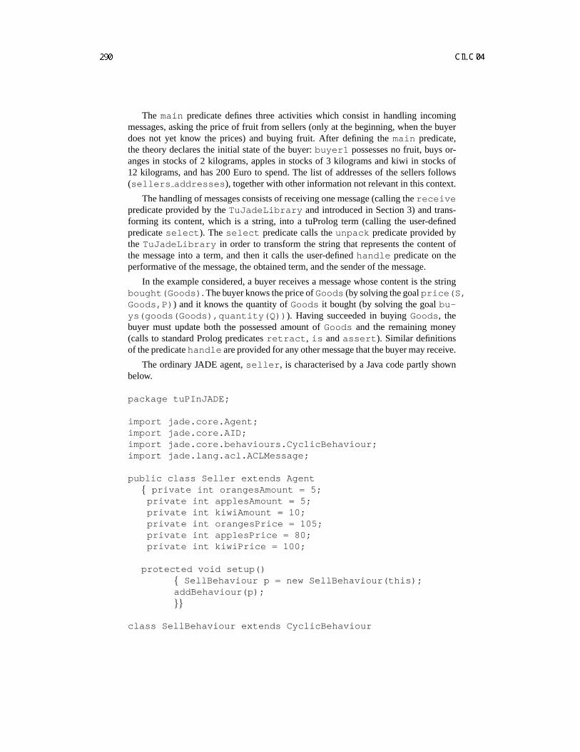
The main predicate defines three activities which consist in handling incomingmessages, asking the price of fruit from sellers (only at the beginning, when the buyerdoes not yet know the prices) and buying fruit. After defining themain predicate,the theory declares the initial state of the buyer:buyer1 possesses no fruit, buys or-anges in stocks of 2 kilograms, apples in stocks of 3 kilograms and kiwi in stocks of12 kilograms, and has 200 Euro to spend. The list of addresses of the sellers follows(sellers addresses ), together with other information not relevant in this context.

The handling of messages consists of receiving one message (calling thereceivepredicate provided by theTuJadeLibrary and introduced in Section 3) and trans-forming its content, which is a string, into a tuProlog term (calling the user-definedpredicateselect ). Theselect predicate calls theunpack predicate provided bythe TuJadeLibrary in order to transform the string that represents the content ofthe message into a term, and then it calls the user-definedhandle predicate on theperformative of the message, the obtained term, and the sender of the message.

In the example considered, a buyer receives a message whose content is the stringbought(Goods) . The buyer knows the price ofGoods (by solving the goalprice(S,Goods,P) ) and it knows the quantity ofGoods it bought (by solving the goalbu-ys(goods(Goods),quantity(Q)) ). Having succeeded in buyingGoods, thebuyer must update both the possessed amount ofGoods and the remaining money(calls to standard Prolog predicatesretract , is andassert ). Similar definitionsof the predicatehandle are provided for any other message that the buyer may receive.

The ordinary JADE agent,seller , is characterised by a Java code partly shownbelow.

package tuPInJADE;

import jade.core.Agent;import jade.core.AID;import jade.core.behaviours.CyclicBehaviour;import jade.lang.acl.ACLMessage;

public class Seller extends Agent private int orangesAmount = 5;

private int applesAmount = 5;private int kiwiAmount = 10;private int orangesPrice = 105;private int applesPrice = 80;private int kiwiPrice = 100;

protected void setup() SellBehaviour p = new SellBehaviour(this);addBehaviour(p);

class SellBehaviour extends CyclicBehaviour

private static boolean done = false;

public SellBehaviour(Agent a) super(a);

public void action() ACLMessage msg;while (!done) msg = myAgent.receive();if (msg != null) handleMsgs(msg);

TheSeller class extends the JADEAgent class as any agent running in JADEmust do. The behaviour of the seller is a cyclic behaviour (classSellBehaviour ex-tendsCyclicBehaviour ) which continuously checks for a message (msg = myA-gent.receive() ) and, if a message is present, handles it (if (msg != null)handleMsgs(msg) ).

Once all the agents have been specified using tuProlog or JADE, they can be loadedinto JADE and the execution of the obtained prototype can start. JADE offers the possi-bility to follow the communication between the agents by means of the “sniffer” agentwhich is a GUI whose output is shown in Figure 6.

Fig. 6.Output of the JADE sniffer agent.

The state of the agents’ mailboxes can be inspected thanks to the introspector agent,a GUI too. Figure 7 shows the state of the mailbox ofbuyer2 . This screen-shot wastaken at the beginning of the simulation; all theINFORMmessages shown are answersto price requests previously issued bybuyer2 to the sellers.

Fig. 7.JADE window showing the communication among agents.

Details on the messages exchanged can also be inspected. Figure 8 shows the re-quest for the price of kiwi sent bybuyer2 to seller1 . Figure 9 shows the answer tothis request.

Fig. 8.Price request frombuyer2 to seller1 .

The execution and monitoring of the prototype, obtained by exploiting the tools pro-vided by JADE, allow the developer to verify whether the agents work well according

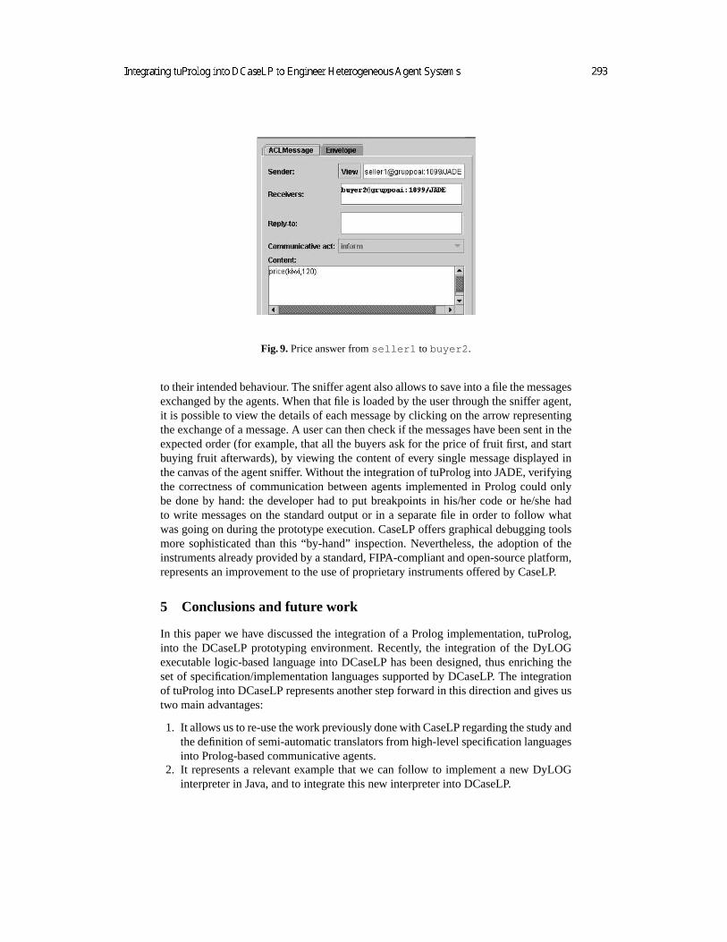
Fig. 9.Price answer fromseller1 to buyer2 .

to their intended behaviour. The sniffer agent also allows to save into a file the messagesexchanged by the agents. When that file is loaded by the user through the sniffer agent,it is possible to view the details of each message by clicking on the arrow representingthe exchange of a message. A user can then check if the messages have been sent in theexpected order (for example, that all the buyers ask for the price of fruit first, and startbuying fruit afterwards), by viewing the content of every single message displayed inthe canvas of the agent sniffer. Without the integration of tuProlog into JADE, verifyingthe correctness of communication between agents implemented in Prolog could onlybe done by hand: the developer had to put breakpoints in his/her code or he/she hadto write messages on the standard output or in a separate file in order to follow whatwas going on during the prototype execution. CaseLP offers graphical debugging toolsmore sophisticated than this “by-hand” inspection. Nevertheless, the adoption of theinstruments already provided by a standard, FIPA-compliant and open-source platform,represents an improvement to the use of proprietary instruments offered by CaseLP.

5 Conclusions and future work

In this paper we have discussed the integration of a Prolog implementation, tuProlog,into the DCaseLP prototyping environment. Recently, the integration of the DyLOGexecutable logic-based language into DCaseLP has been designed, thus enriching theset of specification/implementation languages supported by DCaseLP. The integrationof tuProlog into DCaseLP represents another step forward in this direction and gives ustwo main advantages:

1. It allows us to re-use the work previously done with CaseLP regarding the study andthe definition of semi-automatic translators from high-level specification languagesinto Prolog-based communicative agents.

2. It represents a relevant example that we can follow to implement a new DyLOGinterpreter in Java, and to integrate this new interpreter into DCaseLP.

Currently, the two advantages above cannot be exploited in practice because wedid not have time enough to implement all the components, so we need to make theintegration of DyLOG and the languages provided by CaseLP usable. Our future effortswill be channelled in this implementative direction, in order to make DCaseLP theintegrated environment for engineering and prototyping heterogeneous MAS that it wasintended to be.

References

1. E. Astesiano, M. Martelli, V. Mascardi, and G. Reggio. From Requirement Specification toPrototype Execution: a Combination of a Multiview Use-Case Driven Method and Agent-Oriented Techniques. In J. Debenham and K. Zhang, editors,Proc. of SEKE’03. The Knowl-edge System Institute, 2003.

2. E. Astesiano and G. Reggio. Knowledge Structuring and Representation in RequirementSpecification. InProc. of SEKE’02. ACM Press, 2002.

3. E. Astesiano and G. Reggio. Tight Structuring for Precise UML-based Requirement Specifi-cations: Complete Version. Technical Report DISI–TR–03–06, DISI, Universita di Genova,Italy, 2003.

4. M. Baldoni, C. Baroglio, L. Giordano, A. Martelli, and V. Patti. Reasoning about communi-cating agents in the semantic web. In F. Bry, N. Henze, and J. Maluszynski, editors,Proc. ofPPSWR’03, Springer-Verlag, 2003.

5. M. Baldoni, C. Baroglio, I. Gungui, A. Martelli, M. Martelli, V. Mascardi, V. Patti, andC. Schifanella. Reasoning about agents’ interaction protocols inside DCaseLP. InProc. ofDALT’04. To appear.

6. M. Baldoni, C. Baroglio, A. Martelli, and V. Patti. Reasoning about interaction protocols forweb service composition. In M. Bravetti and G. Zavattaro, editors,Proc. of the WS-FM’04.Elsevier Science Direct, 2004. Electronic Notes in Theoretical Computer Science.

7. M. Baldoni, C. Baroglio, A. Martelli, and V. Patti. Reasoning about logic-based agent inter-action protocols. In this volume.

8. M. Baldoni, L. Giordano, A. Martelli, and V. Patti. Programming rational agents in a modalaction logic. Annals of Mathematics and Artificial Intelligence, Special issue on Logic-BasedAgent Implementation. To appear.

9. F. Bellifemine, G. Caire, A. Poggi, and G. Rimassa. JADE – a white paper. Available athttp://jade.cselt.it/papers/WhitePaperJADEEXP.pdf , 2003.

10. FIPA Specifications.http://www.fipa.org .11. Jess home page.http://herzberg.ca.sandia.gov/jess/ .12. M. Martelli and V. Mascardi. From UML diagrams to Jess rules: Integrating OO and rule-

based languages to specify, implement and execute agents. In F. Buccafurri, editor,Proc. ofAGP’03, 2003.

13. M. Martelli, V. Mascardi, and F. Zini. CaseLP: a prototyping environment for heteroge-neous multi-agent systems. Available athttp://www.disi.unige.it/person/MascardiV/Download/aamas-journal-MMZ04.ps.gz .

14. J. Odell, H. V. D. Parunak, and B. Bauer. Extending UML for agents. InProc. of AOIS’00,2000.

15. SICStus Prolog home page.http://www.sics.se/isl/sicstuswww/site/index.html .

16. TuProlog home page.http://lia.deis.unibo.it/research/tuprolog/ .

Communication Architecture in the DALI LogicProgramming Agent-Oriented Language?

Stefania Costantini Arianna Tocchio Alessia Verticchio

Universita degli Studi di L’AquilaDipartimento di Informatica

Via Vetoio, Loc. Coppito, I-67010 L’Aquila - Italystefcost,tocchio @di.univaq.it

Abstract. In this paper we describe the communication architecture of the DALILogic Programming Agent-Oriented language. We have implemented the rele-vant FIPA compliant primitives, plus others which we believe to be suitable in alogic setting. We have designed a meta-level where: on the one hand the user canspecify, via two distinguished primitives tell/told, constraints on communicationand/or a communication protocol; on the other hand, meta-rules can be definedfor filtering and/or understanding messages via applying ontologies and formsof commonsense and case-based reasoning. These forms of meta-reasoning areautomatically applied when needed by a form of reflection.

1 Introduction

Interaction is an important aspect of Multi-agent systems: agents exchange messages,assertions, queries. This, depending on the context and on the application, can be eitherin order to improve their knowledge, or to reach their goals, or to organize useful coop-eration and coordination strategies. In open systems the agents, though possibly basedupon different technologies, must speak a common language so as to be able to interact.Agent Communication Languages (ACL), such as the widely-adopted FIPA ACL, pro-vide standardized catalogues of performatives (communication acts), designed in orderto ensure interoperability among agent systems [12].

However, beyond standard forms of communication, the agents should be capableof filtering and understanding message contents. A well-understood topic is that of in-terpreting the content by means of ontologies, which are essentially dictionaries anddescriptions that allow different terminologies to be coped with. In a logic language,the use of ontologies can be usefully integrated with forms of commonsense and case-based reasoning, that improve the “understanding” capabilities of an agent. A moresubtle point is that it would be useful for an agent to have the possibility to enforce con-straints on communication. This implies being able to accept or refuse or rate a message,based on various conditions like for instance the degree of trust in the sender. This alsoimplies to be able to follow a communication protocol in “conversations”. Since thedegree of trust, the protocol, the ontology, and other factors, can vary with the context,

? We acknowledge support by theInformation Society Technologies programme of the EuropeanCommission, Future and Emerging Technologiesunder the IST-2001-37004 WASP project.

or can be learned from previous experience, in a logic language agent should and mightbe able to perform meta-reasoning on communication, so as to interact flexibly with the“external world.”

This paper presents the communication architecture of the DALI language. DALIis an Agent-Oriented Logic Programming language designed for executable specifica-tion of logical agents, that allows one to define one or more agents interacting amongthemselves, with other software entities and with an external environment. A main de-sign objective for DALI has been that of introducing in a declarative fashion all theessential features, while keeping the language as close as possible to the syntax andsemantics of the traditional Horn-clause language. In practice, most Prolog programscan be understood as DALI programs. Special atoms and rules have been introduced forrepresenting: external events, to which the agent is able to respond (reactivity); actions(reactivity and proactivity); internal events (previous conclusions which can trigger fur-ther activity); past and present events (to be aware of what has happened), goals (thatthe agent can reach). Then, on the line of the arguments proposed in [10], DALI is anenhanced logic language with fully logical semantics [5], that integrates rationality andreactivity, where an agent is able of both backwards and forward reasoning, and has thecapability to enforce “maintenance goals” that preserve her internal state, and “achieve-ment goal” that pursue more specific objectives. An extended resolution is provided,so that the DALI interpreter is able to answer queries like in the plain Horn-clauselanguage, but is also able to cope with the different kinds of events.

We have introduced in DALI a communication architecture that specifies in a flexi-ble way the rules of interaction among agents, according to the above-mentioned crite-ria. The various aspects are modeled in a declarative way, are adaptable to the user andapplication needs, and can be easily composed. Basically, DALI agents communicatevia FIPA ACL, augmented with some primitives which are suitable for a logic lan-guage. As a first layer of the architecture, we have introduced a check level that filtersthe messages. This layer verifies that the message respects the communication protocolof the agent, as well as some domain-independent coherence properties. Several otherproperties to be checked can be however additionally specified, by expanding the defi-nition of the distinguished predicatestell/told. If the message does not pass the check,it is deleted and does not produce any effect. As a second layer, meta-level reasoningis exploited so as to try to understand messages coming from other software entities byusing ontologies, and forms of commonsense reasoning.

In summary, when a DALI agent receives a message by another agent, the messageis submitted to a check level that controls if it respects the communication protocoland the conditions expressed by the check rules. If the message gets over this control,the agent invokes meta-level reasoning in order to understand its content. The meta-reasoning process uses the agent’s ontology and other properties of the terms occurringin the message.

It is important to notice that the definition of the enhanced DALI/FIPA ACL isimported by the agent’s code as a library, so as in principle DALI agents may adopt dif-ferent communication protocols. Also, checks and constraints on communication canbe modified without affecting (or without even knowing) the agent’s code. The lay-ers of message check and understanding have a predefined default part. However, as

2

mentioned before they can be extended, improved and adapted to the specific user orapplication needs by adding rules to the definition of some distinguished predicated.

In this paper we will not be concerned with formal aspects. Rather, we mean toillustrate the communication architecture, and to demonstrate its usefulness mainly bymeans of significant examples.

The paper is organized as follows. We start by shortly describing the main featuresof DALI in Section 2. In Section 3 we discuss the new DALI/FIPA protocol and inSection 4 we introduce DALI communication filter. Then, in Sections 5 and 6 we sum-marize the meta-reasoning layer and how the new architecture works. In Section 7 weshow an example of communication between DALI agents, and then conclude in Sec-tion 8 with some final remarks.

2 The DALI language

DALI [4] [5] is an Active Logic Programming language designed for executable spec-ification of logical agents. A DALI agent is a logic program that contains a particularkind of rules, reactive rules, aimed at interacting with an external environment. Theenvironment is perceived in the form of external events, that can be exogenous events,observations, or messages by other agents. In response, a DALI agent can perform ac-tions, send messages, invoke goals. The reactive and proactive behavior of the DALIagent is triggered by several kinds of events: external events, internal, present and pastevents. It is important to notice that all the events and actions are timestamped, so as torecord when they occurred. The new syntactic entities, i.e., predicates related to eventsand proactivity, are indicated with special postfixes (which are coped with by a pre-processor) so as to be immediately recognized while looking at a program.

2.1 External Events

The external events are syntactically indicated by the postfixE. When an event comesinto the agent from its “external world”, the agent can perceive it and decide to react.The reaction is defined by a reactive rule which has in its head that external event.The special token:>, used instead of: −, indicates that reactive rules performs forwardreasoning. E. g., the body of the reactive rule below specifies the reaction to the externaleventbell ringsE that is in the head. In this case the agent performs an action, postfixA, that consists in opening the door.

bell ringsE :> open the doorA.

The agent remembers to have reacted by converting the external event into apast event(time-stamped).

Operationally, if an incoming external event is recognized, i.e., corresponds to thehead of a reactive rule, it is added into a list called EV and consumed according to thearrival order, unless priorities are specified. Priorities are listed in a separate file of di-rectives, where (as we will see) the user can “tune” the agent’s behaviour under severalrespect. The advantage introducing a separate initialization file is that for modifying thedirectives there is no need to modify (or even to understand) the code.

3

2.2 Internal Events

The internal events define a kind of “individuality” of a DALI agent, making her proac-tive independently of the environment, of the user and of the other agents, and allowingher to manipulate and revise her knowledge [3]. An internal event is syntactically in-dicated by the postfixI, and its description is composed of two rules. The first onecontains the conditions (knowledge, past events, procedures, etc.) that must be true sothat the reaction (in the second rule) may happen.

Internal events are automatically attempted with a default frequency customizableby means of directives in the initialization file. The user’s directives can tune severalparameters: at which frequency the agent must attempt the internal events; how manytimes an agent must react to the internal event (forever, once, twice,. . . ) and when (for-ever, when triggering conditions occur, . . . ); how long the event must be attempted(until some time, until some terminating conditions, forever).

For instance, consider a situation where an agent prepares a soup that must cookon the fire for K minutes. The predicates with postfixP are past events, i.e., events oractions that happened before, and have been recorded. Then, the first rule says that thesoup is ready if the agent previously turned on the fire, and K minutes have elapsedsince when she put the pan on the stove. The goalsoupreadywill be attempted fromtime to time, and will finally succeed when the cooking time will have elapsed. At thatpoint, the agent has to react to this (by second rule) thus removing the pan and switchingoff the fire, which are two actions (postfixA).

soup ready : − turn on the fireP, put pan on the stoveP : T,cooking time(K), time elapsed(T, K).

soup readyI :> take off pan from stoveA, turn off the fireA.

A suitable directive for this internal event can for instance state that it shouldbe attempted every 60 seconds, starting from whenput the pan on the stove andturn on the fire have become past events.

Similarly to external events, internal events which are true by first rule are insertedin a set IV in order to be reacted to (by their second rule). The interpreter, interleavingthe different activities, extracts from this set the internal events and triggers the reaction(again according to priorities). A particular kind of internal event is thegoal, postfixG,that stop being attempted as soon as it succeeds for the first time.

2.3 Present Events

When an agent perceives an event from the “external world”, it doesn’t necessarilyreact to it immediately: she has the possibility of reasoning about the event, before (orinstead of) triggering a reaction. Reasoning also allows a proactive behavior. In thissituation, the event is called present event and is indicated by the suffixN.

2.4 Actions

Actions are the agent’s way of affecting her environment, possibly in reaction to anexternal or internal event. In DALI, actions (indicated with postfixA) may have or not

4

preconditions: in the former case, the actions are defined by actions rules, in the lattercase they are just action atoms. An action rule is just a plain rule, but in order to empha-size that it is related to an action, we have introduced the new token:<, thus adoptingthe syntaxaction :< preconditions. Similarly to external and internal events, actionsare recorded as past actions.

2.5 Past events

Past events represent the agent’s “memory”, that makes her capable to perform its fu-ture activities while having experience of previous events, and of its own previous con-clusions. As we have seen in the examples, past event are indicated by the postfixP.For instance,alarm clock ringsP is an event to which the agent has reacted and whichremains in the agent’s memory. Each past event has a timestamp T indicating when therecorded event has happened. Memory of course is not unlimited, neither conceptuallynor practically: it is possible to set, for each event, for how long it has to be kept inmemory, or until which expiring condition. In the implementation, past events are keptfor a certain default amount of time, that can be modified by the user through a suitabledirective in the initialization file. Implicitly, if a second version of the same past eventarrives, with a more recent timestamp, the older event is overridden, unless a directiveindicates to keep a number of versions.

3 DALI/FIPA Agent Communication Language

An agent communication language (ACL) is a set of primitives and rules that guidethe interaction among several agents [7]. There are a number of standardized languagesthat the agents can use for communication. The most widely acknowledged is the FIPAACL, which for the sake of interoperability we have adopted (with few extensions) forDALI. The specification of FIPA messages has the following structure:

– receiver:name of the agent that receives the message;– language:the language in which the message is expressed;– ontology: the vocabulary of the words in the message, or, more generally, the de-

scription of conceptual relationships between terms and sentences of the same do-main, which are expressed in a different terminology;

– sender:name of the agent that sends the message;– content: the content of the message, which is the main part, discussed in detail

below.

In DALI, a message which has to be sent has the format:

primitive(content)

whereprimitive is what is called acommunication performative, i.e., the specificationof the intended meaning of the message, which is then further specified bycontent.For instance,propose(content)is a performative aimed at asking another agent to dosomething, where what should be done is specified bycontent. The DALI interpreter

5

automatically adds the missing FIPA parameters, thus creating the structure which isactually sent, i.e.:

message( receiver address, receiver name, sender address, sender name,language, ontology, primitive(content, sender))

Symmetrically, from a message which is received the interpreter extracts the partprimitive(Content,Sender), that is what the receiver agent has to consider. In most cases,the receiver will record the itemprimitive(Content,Sender)as a past event. Please noticethatcontentmay be a conjunction, as the FIPA performatives have different arities.

In the rest of this section, we illustrate the main performatives we adopt. In bracketswe indicate if the primitive is FIPA or if it is peculiar of DALI. In most cases, thereceiver will record the itemprimitive(Content,Sender)as a past event.

sendmessage(DALI)

send message(external event, sender agent)

The act of sending a message to a DALI agent that the receiver will perceive as thecommunication that the given external event has happened.

propose(FIPA)

propose(action, [precondition1, ..., preconditionn], sender agent).

The act of asking another agent to perform a certain action, given certain preconditions.A DALI agent accepts a proposal if the preconditions are all true, else she rejects theproposal.

acceptproposal (FIPA)

accept proposal( action accepted, [condition1, ..., conditionn], sender agent)oraccept proposal( action accepted, [condition1, ..., conditionn], in response to(),

sender agent)

The action of accepting a previously received proposal to perform an action where thethe conditions of the agreement are enclosed.

reject proposal (FIPA)

reject proposal( action rejected, [reason1, ..., reasonn], sender agent)orreject proposal( action rejected, [reason1, ..., reasonn], in response to(),

sender agent)

The action of rejecting a proposal to perform some action during a negotiation, listingthe reasons for rejection.

failure (FIPA)

failure(action failed, motivation, sender agent)

The action of telling another agent that an action was attempted but the attempt failed,enclosing the motivation of the failure.

cancel(FIPA)

cancel(action to cancel, sender agent).

The action of canceling some previously requested action which had a temporal extent(i.e. cannot be instantaneous).

6

executeproc (DALI)

execute proc(call procedure, sender agent).

The act of invoking a procedure inside a DALI program.

query ref (FIPA)

query ref(property, N, sender agent)

The action of asking another agent for the object referred to by an expression containingfree variables.Propertyis the string on which the matching is attempted, and N is therequested number of matches for the object to be identified.

inform (FIPA)

inform(something, sender agent) orinform(primitive, values/motivation, sender agent)

The sender informs the receiver that a certain “something” is happened.

is a fact (DALI)

is a fact(proposition, sender agent)

The act of asking if the proposition indicated in the primitive is true.

refuse(FIPA)

refuse(action refused, motivation, sender agent)

The action of refusing to perform a given action, and of explaining the reason for therefusal. For example,a DALI agent refuses to do an action if the preconditions of thecorresponding active rules in the DALI logic program are false. The refusal is recordedas a past event.

confirm (FIPA)

confirm(proposition, sender agent)

The sender informs the receiver that a given proposition is true, where the receiver issupposed to be uncertain about the proposition. The proposition is asserted as a pastevent.

disconfirm (FIPA)

disconfirm(proposition, sender agent)

The sender informs the receiver that a given proposition is false, where the receiver isinstead supposed to believe that the proposition is true. Then, this proposition is deletedfrom past events.

4 DALI communication filter

In real applications, the interaction between agents raises the problem of security. Ifan agent is not sufficiently self-defending, she can suffer from damages to either herknowledge base or her rules. It may happen in fact that an agent sends to another one amessage with a wrong content, intentionally or not, thus potentially bringing a seriousdamage. How to recognize a correct message? And a wrong message?

7

The solution adopted in DALI is aimed at providing a tool for coping, as far as pos-sible, with these problems. When a message is received, it is examined by a check layercomposed of a structure which is adaptable to the context and modifiable by the user.This filter checks the content of the message, and verifies if the conditions for the recep-tion are verified. If the conditions are false, this security level eliminates the supposedlywrong message. We have constrained the reception of messages by restricting the rangeof allowed utterances to the FIPA/DALI primitives, according to additional conditionsdefined by the user, or, in perspective, learned by the agent herself. For instance, filteringconditions can be based upon reliability of the sender agent. The DALI filter is spec-ified by means of meta-level rules defining the distinguished predicatestell and told.These meta-rules are contained in a separate file, and can be changed without affectingor even knowing the DALI code. Then, communication in DALI is elaboration-tolerantwith respect to both the protocol, and the filter.

4.1 Filter for the incoming messages

Whenever a message is received, with content partprimitive(Content,Sender)the DALIinterpreter automatically looks for a correspondingtold rule, which is of the form:

told(Sender, primitive(Content)) : −constraint1, . . . , constraintn.

whereconstraint i can be everything expressible either in Prolog or in DALI. Ifsuch a rule is found, the interpreter attempts to prove told(Sender, primitive(Content)).If this goal succeeds, then the message is accepted, and primitive(Content)) is added tothe set of the external events incoming into the receiver agent. Otherwise, the messageis discarded. Semantically, this can be understood as implicit reflection up to the filterlayer, followed by a reflection down to whatever activity the agent was doing, with orwithout accepting the message. For a detailed and general semantic account of this kindof reflection, the reader may refer to [1].

Below we propose a number of examples of filtering rules. Notice that each agentcan have her own set of filtering rules. Since she takes these rules from a separate file,her filtering criteria can vary (by importing a different file) according to the context sheis presently involved into.

The following rule accepts asendmessageprimitive if the receiver agent remem-bers (presumably from past experience) that the sender is reliable, and believes that thecontent is worth knowing.

told( Sender agent, send message(External event)) : −not(unreliableP (Sender agent)), interesting(External event).

Similarly, the request of either executing a procedure or asserting a fact is takeninto consideration if the agent who is asking us is reliable, and in the former case if weactually have the code of that procedure, in the latter case if we are interested in the newfact.

told( Sender agent, execute proc(Procedure)) : −not(unreliableP (Sender agent)), know(Procedure).

told( Sender agent, is a fact(Proposition)) : −not(unreliableP (Sender agent)), interesting(Proposition).

8

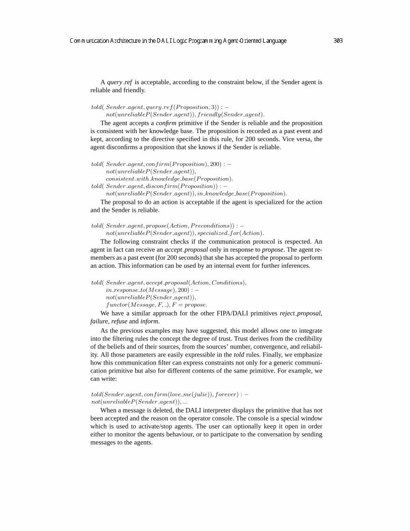
A query ref is acceptable, according to the constraint below, if the Sender agent isreliable and friendly.

told( Sender agent, query ref(Proposition, 3)) : −not(unreliableP (Sender agent)), friendly(Sender agent).

The agent accepts aconfirmprimitive if the Sender is reliable and the propositionis consistent with her knowledge base. The proposition is recorded as a past event andkept, according to the directive specified in this rule, for 200 seconds. Vice versa, theagent disconfirms a proposition that she knows if the Sender is reliable.

told( Sender agent, confirm(Proposition), 200) : −not(unreliableP (Sender agent)),consistent with knowledge base(Proposition).

told( Sender agent, disconfirm(Proposition)) : −not(unreliableP (Sender agent)), in knowledge base(Proposition).

The proposal to do an action is acceptable if the agent is specialized for the actionand the Sender is reliable.

told( Sender agent, propose(Action, Preconditions)) : −not(unreliableP (Sender agent)), specialized for(Action).

The following constraint checks if the communication protocol is respected. Anagent in fact can receive anacceptproposalonly in response topropose. The agent re-members as a past event (for 200 seconds) that she has accepted the proposal to performan action. This information can be used by an internal event for further inferences.

told( Sender agent, accept proposal(Action, Conditions),in response to(Message), 200) : −not(unreliableP (Sender agent)),functor(Message, F, ), F = propose.

We have a similar approach for the other FIPA/DALI primitivesreject proposal,failure, refuseandinform.

As the previous examples may have suggested, this model allows one to integrateinto the filtering rules the concept the degree of trust. Trust derives from the credibilityof the beliefs and of their sources, from the sources’ number, convergence, and reliabil-ity. All those parameters are easily expressible in thetold rules. Finally, we emphasizehow this communication filter can express constraints not only for a generic communi-cation primitive but also for different contents of the same primitive. For example, wecan write:

told(Sender agent, confirm(love me(julie)), forever) : −not(unreliableP (Sender agent)), ...

When a message is deleted, the DALI interpreter displays the primitive that has notbeen accepted and the reason on the operator console. The console is a special windowwhich is used to activate/stop agents. The user can optionally keep it open in ordereither to monitor the agents behaviour, or to participate to the conversation by sendingmessages to the agents.

9

4.2 Filter layer for outcoming messages

Symmetrically totold rules, the messages that an agent sends are subjected to a checkvia tell rules. There is, however, an important difference: the user can choose whichmessages must be checked and which not. The choice is made by setting some param-eters in the initialization file. The syntax of atell rule is:

tell(Receiver, Sender, primitive(Content)) : −constraint1, . . . , constraintn

For every message that is being sent, the interpreter automatically checks whetheran applicabletell rule exists. If so, the message is actually sent only upon success of thegoaltell(Receiver, Sender, primitive(Content)).

Below we show as an example two of the default rules coping with the DALI/FIPAprimitives. The firsttell rule authorizes the agent to send the message with the primitiveinform if the receiver is active in the environment and is presumably interested to theinformation: via rules like this one we can considerably reduce useless exchange ofmessages. According to the second rule, the agent sends arefuseonly if the requestedprimitive is is a fact or query ref.

tell( Agent To, Agent From, inform(Proposition)) : −active in the world(Agent To),specialized(Agent To, Specialization),related to(Specialization, Proposition).

tell( Agent To, Agent From, refuse(Something, Motivation)) : −arg(1, Something, Primitive),functor(Primitive, F ), (F = is a fact; F = query ref).

5 Meta-reasoning layer

In heterogeneous Multi-agent Systems, in general not all the components speak thesame language, and not all of them use the same words to express a concept. The agentthat doesn’t understand a proposition can either accept the defeat and ignore the mes-sage, or try to apply a reasoning process in order to interpret the message contents. Thelatter solution can be more easily put at work by taking advantage of meta-reasoningcapabilities of a logic language. In fact, the use ofontologies, which are dictionariesof equivalent terms, can be integrated with several kinds of commonsense reasoning.The ontology of a DALI agent is in a file .txt containing equivalent terms and otherproperties useful in the meta-reasoning process. E.g., agentbob’s ontology can be thefollowing, wheresymmetricis a property of relations, which is asserted to hold of predi-catefriend), and allows him to conclude bothfriend(bob,lucy)andfriend(lucy,bob)evenif originally he could derive only one. The name of the agent enclosed to each item ofthe ontology allows a group of agents to use the same ontology file, though sharing thecontents only partially.

ontology(bob, rain, water falling from sky).ontology(bob, friend, amico).. . . symmetric(friend).

10

Each DALI agent is provided (again in a separate file) with a distinguished pro-cedure calledmeta, to support the meta-reasoning process. This procedure by defaultincludes a number of rules for coping with domain-independent standard situations. Theuser can add other rules, thus possibly specifying domain-dependent commonsense rea-soning strategies for interpreting messages, or implementing a learning strategy to beapplied when all else fails. Below we report some of the default meta-reasoning rulesthat apply the equivalences listed in the ontology, and possibly also exploit symmetry(for binary predicates only):

meta( Initial term, F inal term, Agent Sender) : −clause(agent(Agent Receiver), ),functor(Initial term, Functor, Arity), Arity = 0,((ontology(Agent Sender, Functor, Equivalent term);ontology(Agent Sender, Equivalent term, Functor));(ontology(Agent Receiver, Functor, Equivalent term);ontology(Agent Receiver, Equivalent term, Functor))),F inal term = Equivalent term.

. . .meta( Initial term, F inal term, Agent Sender) : −

functor(Initial term, Functor, Arity), Arity = 2,symmetric(Functor), Initial term = ..List,delete(List, Functor, Result list),reverse(Result list, Reversed list),append([Functor], Reversed list, F inal list),F inal term = ..F inal list.

The procedure meta is automatically invoked, again via reflection, by the interpreter.It is necessary to avoid unwanted variable bindings while meta-reasoning about mes-sages. In DALI, message contents are always reified, i.e., transformed into a groundterm, before they are sent, and thus they are received in reified form. Then, the inter-preter includes facilities for “reification”, or “naming”, and “de-reification”, or “un-naming” of language expressions (also this issue is discussed at length in [1]).

6 DALI Communication Architecture

In this section we summarize the overall DALI communication architecture, that putstogether the functionalities of filter, meta-reasoning and the protocol layers. The archi-tecture consists of three levels: the first level implements the protocol and the filter,i.e., the first two layers of the communication structure; the second level includes themeta-reasoning layer; the third level consists of the DALI interpreter, which is able toactivate the agents. Each agent is defined by a .txt file, containing the agent code writtenin DALI. When an agent receives an external event through the primitivesendmessage,the DALI interpreter calls the filter layer by invoking its internal rule:

receive( send message(External event, Agent Sender)) : −told(Agent Sender, send message(External event)), ...

If the message overcomes the security check, then the interpreter automatically in-vokes the meta-level in order to understand the external event. The meta reasoning pro-

11

cess initially has to “un-name” the message content, so as to verify if (an instance of)Externaleventbelong to the set of external events known by the agent without applyingthe meta procedure. If it is the case, then the agent reacts directly, else the interpretertakes advantage of meta reasoning capabilities for finally finding a reactive rule of thelogic program applicable to the context.

Similarly, the meta reasoning level is called for the primitives:propose, exe-cuteproc, query ref andis a fact. The proceduremetain fact contains a special rule foreach different communication act. E. g., the code for the primitiveproposeis reportedbelow: if the action proposed belong to the actions occurring in the logic program ofagent, then the interpreter sends back to the proposer agent a messageacceptproposal,else areject proposal.

receive(propose( Action, Conditions, Sender Agent)) : −told(Sender Agent, propose(Action, Conditions)), . . . ,call meta propose(Action, Conditions, Sender Agent).

call meta propose( Action, Conditions, Sender Agent) : −once(call propose(Action, Conditions, Sender Agent)).

call propose( Action, Conditions, Sender Agent) : −denaming(Action, New action), exists action(New action),execute propose(New action, Conditions, Sender Agent).

call propose( Action, Conditions, Sender Agent) : −meta(Action, New term, ), denaming(New term, New action),exists action(New action),execute propose(New action, Conditions, Sender Agent).

In the first rule ofcall proposethe interpreter, after the de-naming of the term, ver-ifies whether the agent knows the action, without applying either the ontology or otherproperties. In the second rule, called if the first one fails, the interpreter changes thename of the action by applying the meta reasoning and, after the de-naming, checksagain if (an instance of) the required action exists among those feasible by the agent.The link with the part of the DALI interpreter that handles events, goals and actions isrepresented by the procedureexecutepropose. Via this procedure the action, if recog-nized, is put into the queue of actions that are waiting to be executed.

7 Example: an Italian client in an English pub

We propose an example of interaction between DALI agents employing the communi-cation architecture that we have discussed. We consider four agents: (i)agent waiter:he is a pub (or cafeteria) waiter that receives orders and serves drinks to clients; (ii)agentgino: an italian client, who walks into the cafeteria and orders a beer incorrectly;(iii) agentwife: wife of another client,bob, who is a drunkard and never finds his wayhome; (iv)agentfriend: friend of the italian clientgino.

The italian clientgino walks into the pub and orders a beer, mixing Italian andEnglish languages and mispelling the wordbeer. He sends to the waiter the message:

send message(voglio(gino, ber), gino).

12

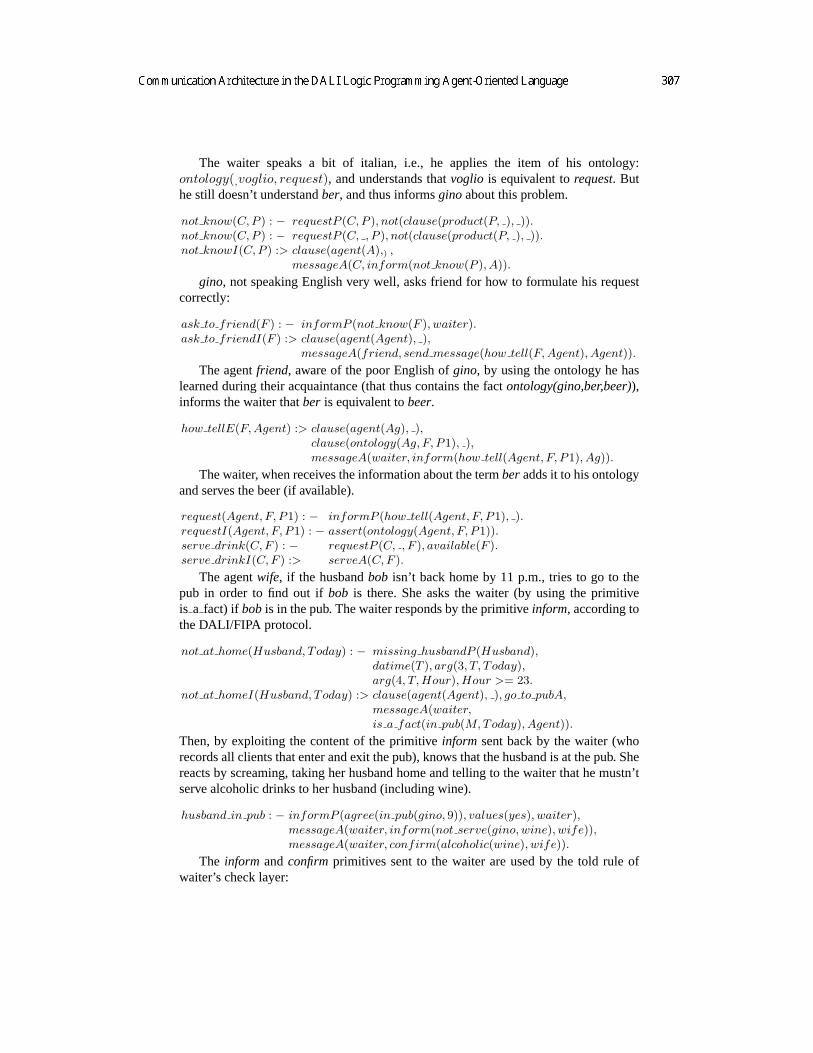
The waiter speaks a bit of italian, i.e., he applies the item of his ontology:ontology(,voglio, request), and understands thatvoglio is equivalent torequest. Buthe still doesn’t understandber, and thus informsginoabout this problem.

not know(C, P ) : − requestP (C, P ), not(clause(product(P, ), )).not know(C, P ) : − requestP (C, , P ), not(clause(product(P, ), )).not knowI(C, P ) :> clause(agent(A),) ,

messageA(C, inform(not know(P ), A)).

gino, not speaking English very well, asks friend for how to formulate his requestcorrectly:

ask to friend(F ) : − informP (not know(F ), waiter).ask to friendI(F ) :> clause(agent(Agent), ),

messageA(friend, send message(how tell(F, Agent), Agent)).

The agentfriend, aware of the poor English ofgino, by using the ontology he haslearned during their acquaintance (that thus contains the factontology(gino,ber,beer)),informs the waiter thatber is equivalent tobeer.

how tellE(F, Agent) :> clause(agent(Ag), ),clause(ontology(Ag, F, P1), ),messageA(waiter, inform(how tell(Agent, F, P1), Ag)).

The waiter, when receives the information about the termberadds it to his ontologyand serves the beer (if available).

request(Agent, F, P1) : − informP (how tell(Agent, F, P1), ).requestI(Agent, F, P1) : − assert(ontology(Agent, F, P1)).serve drink(C, F ) : − requestP (C, , F ), available(F ).serve drinkI(C, F ) :> serveA(C, F ).

The agentwife, if the husbandbob isn’t back home by 11 p.m., tries to go to thepub in order to find out ifbob is there. She asks the waiter (by using the primitiveis a fact) if bobis in the pub. The waiter responds by the primitiveinform, according tothe DALI/FIPA protocol.

not at home(Husband, Today) : − missing husbandP (Husband),datime(T ), arg(3, T, Today),arg(4, T, Hour), Hour >= 23.

not at homeI(Husband, Today) :> clause(agent(Agent), ), go to pubA,messageA(waiter,is a fact(in pub(M, Today), Agent)).

Then, by exploiting the content of the primitiveinform sent back by the waiter (whorecords all clients that enter and exit the pub), knows that the husband is at the pub. Shereacts by screaming, taking her husband home and telling to the waiter that he mustn’tserve alcoholic drinks to her husband (including wine).

husband in pub : − informP (agree(in pub(gino, 9)), values(yes), waiter),messageA(waiter, inform(not serve(gino, wine), wife)),messageA(waiter, confirm(alcoholic(wine), wife)).

The inform andconfirmprimitives sent to the waiter are used by the told rule ofwaiter’s check layer:

13

told( Ag, send message(request(Ag, P ))) : −not(informP (not serve(Ag, P ), wife)), alcoholicP (P ).

When the drunkard husband will ask for an alcoholic drink in the future, the mes-sage will be eliminated.

8 Conclusions

This paper has discussed how communication has been designed and implemented inthe DALI Logic Programming Agent-Oriented language. We have shown the kinds ofinteraction and the abstract roles that the DALI/FIPA protocol supports and the func-tionalities of the check and meta-reasoning layers. We have noticed that the proposedarchitecture takes profit of features which are proper of logic languages, such as meta-reasoning and logical reflection.

There are other FIPA-compliant agent frameworks. A future aim of our experimentsin fact is that of ensuring interoperability between DALI and these other approaches.A relevant one is JADE, a FIPA-compliant framework fully developed in Java. Eachagent platform, written in Java and importing the JADE libraries, can be split on sev-eral hosts. Each agent is implemented as a Java thread, and Java events are used foreffective and light-weight communication between agents on the same host. A num-ber of FIPA-compliant DFs (Directory Facilitators) agents can be started at run time inorder to implement multi-domain applications. About security, JADE provides propermechanisms to authenticate and verify the rights assigned to agents. [2]

The 3APL platform is the first platform that has supported easy and direct imple-mentation and execution of cognitive agents. The platform can be distributed acrossdifferent machines connected in a network. Moreover, the 3APL platform is FIPA com-pliant in the sense that agents running on this platform can in principle communicatewith agents that run on a different FIPA compliant platforms such as JADE. [11]

However, the DALI project demonstrates that a logic programming language with alogic semantics [5] is able to exhibit, also for communication, features that are as pow-erful (and even more flexible) as those of approaches that are either not fully logical,or semantically more complex. The DALI implementation cannot currently competein efficiency with others like JADE, which have been developed in the industry, andon which a lot of effort has been spent by several companies and universities. Never-theless, DALI is competitive from the point of view of the ease and flexibility of use,for every kind of application, but especially where context-sensitivity, adaptability andintelligence are needed. We have equipped DALI with an interface with Java, that hasallowed us to develop applications (namely in component management and reconfigura-tion in distributed systems [3] ) where the Java part is able to interact at a low level withlegacy systems, and the DALI part implements intelligent reasoning and sophisticatedinteraction. The declarative semantics of DALI has been defined in [5]. The operationalsemantics is being defined in a Ph.D. Thesis. The behaviour of DALI interpreter hasbeen modeled and checked by using the Murφ model checker [9]. A future aim of thisresearch is that of developing and experimenting cooperative models for DALI logicalagents, also based on game theory. As a first step, we are studying formal models for

14

making DALI agents adaptive with respect to the level of trust that they assign to theother agents.

References

1. J. Barklund, S. Costantini, P. Dell’Acqua e G. A. Lanzarone,Reflection Principles inComputational Logic, Journal of Logic and Computation, Vol. 10, N. 6, December 2000,Oxford University Press, UK.

2. F. Bellifemine, A. Poggi, G. Rimassa,JADE: A FIPA-compliant agent framework, In: Proc.of the 4th International Conference and Exhibition on The Pratical Application of IntelligentAgents and Multiagents, held in London,UK, December 1999.

3. M. Castaldi, S. Costantini, S. Gentile, A. Tocchio,A Logic-Based Infrastructure for Recon-figuring Applications, In: J. A. Leite, A. Omicini. L. Sterling, P. Torroni (eds.),DeclarativeAgent Languages and Technologies, Proc. of the 1st International Workshop, DALT 2003(held in Melbourne, Victoria, July 2003), Available also on-line, URLhttp://centria.di.fct.unl.pt/ jleite/dalt03/papers/dalt2003proceedings.pdf.

4. S. Costantini. Towards active logic programming. In A. Brogi and P. Hill, editors,Proc. of2nd International Workshop on component-based Software Development in ComputationalLogic (COCL’99), PLI’99, (held in Paris, France, September 1999), Available on-line, URLhttp://www.di.unipi.it/ brogi/ResearchActivity/COCL99/proceedings/index.html.

5. S. Costantini and A. Tocchio,A Logic Programming Language for Multi-agent Systems,In S. Flesca, S. Greco, N. Leone, G. Ianni (eds.),Logics in Artificial Intelligence, Proc. ofthe 8th Europ. Conf., JELIA 2002, (held in Cosenza, Italy, September 2002), LNAI 2424,Springer-Verlag, Berlin, 2002.

6. U. Endriss, N. Maudet, F. Sadri, F. Toni,Logic-based Agent Communication Protocols,In: Lecture Notes in Computer Science, Advances in Agent Communication, Proc. of theInternational Workshop on Agent Communication Languages ACL03, (held in Melbourne,Australia, July 14 2003), LNCS 2922, Springer-Verlag, Berlin, 2004.

7. M.-P. Huget, J.-L. Koning,Interaction Protocol Engineering, In: Lecture Notes in ComputerScience, Communication in Multiagent Systems, Agent Communication Languages and Con-versation Policies, LNCS 2650, Springer-Verlag, Berlin, 2003.

8. M. N. Huhns, L. M. Stephens,Multiagent System and Societies of Agents, In: MultiagentSystems: A modern Approach to Distributed Artificial Intelligence, 1999.

9. B. Intrigila, I. Melatti, A. Tocchio,Model-checking DALI with Murφ, Tech. Rep., Univ. ofL’Aquila, 2004.

10. R. A. Kowalski,How to be Artificially Intelligent - the Logical Way, Draft, revised February2004, Available on line, URLhttp://www-lp.doc.ic.ac.uk/UserPages/staff/rak/rak.html.

11. E.C. Van der Hoeve, M. Dastani, F. Dignum, J.-J. Meyer,3APL Platform, In: Proc. of the The15th Belgian-Dutch Conference on Artificial Intelligence(BNAIC2003), held in Nijmegen,The Netherlands, 2003.

12. J. M. Serrano, S. Ossowski.An Organisational Approach to the Design of Interaction Pro-tocols, In: Lecture Notes in Computer Science, Communications in Multiagent Systems:Agent Communication Languages and Conversation Policies, LNCS 2650, Springer-Verlag,Berlin, 2003.

15

Preserving (Security) Properties under ActionRefinement?

Annalisa Bossi, Carla Piazza, and Sabina Rossi

Dipartimento di Informatica, Universita Ca’ Foscari di Veneziavia Torino 155, 30172 Venezia, Italy

bossi,piazza,srossi@dsi.unive.it

Abstract. In the design process of distributed systems we may haveto replace abstract specifications of components by more concrete speci-fications, thus providing more detailed design information. In the contextof process algebra this well-known approach is often referred to as actionrefinement. In this paper we study the relationships between action re-finement, compositionality, and (security) process properties within theSecurity Process Algebra (SPA). We formalize the concept of action re-finement both as a structural inductive definition and in terms of sub-sequent context compositions. We study compositional properties of ournotion of refinement and provide conditions under which general processproperties are preserved through it. Finally, we consider information flowsecurity properties and define decidable classes of secure terms which areclosed under action refinement.

1 Introduction

In the development of complex systems it is common practice to first describeit succinctly as a simple abstract specification and then refine it stepwise to amore concrete implementation. This hierarchical specification approach has beensuccessfully developed for sequential systems where abstract-level instructionsare expanded until a concrete implementation is reached (see, e.g., [21]).

In the context of process algebra, this refinement methodology amounts todefining a mechanism for replacing abstract actions with more concrete pro-cesses. We adopt the terminology action refinement to refer to this stepwisedevelopment of systems specified as terms of a process algebra. We refer to [14]for a survey on the state of the art of action refinement in process algebra.

Action refinement in process algebras is usually defined by extending thesyntax with some compositional operator [1, 13]. Here we follow a different ap-proach and instead of extending the language, we use a construction based oncontext composition. This allows us to reason on the relationships between ac-tion refinement and the security properties of SPA processes that we have deeplystudied in, e.g., [3]. In the last part of the paper we prove that our definition ofaction refinement is indeed equivalent to the one presented in [1].? This work has been partially supported by the EU Contract IST-2001-32617 “Models

and Types for Security in Mobile Distributed Systems” (MyThS).

In this paper we model action refinement as a ternary function Ref taking asarguments an action r to be refined, a system description E on a given level ofabstraction and an interpretation of the action r on this level by a more concreteprocess F on a lower abstraction level. The refined process can be obtained eitherby applying a structural inductive definition or through a more complex contextcomposition as described by the following simple example.

Let E be the process a.r.b.0 + c.0 and r be the action we intend to refine bythe process F ≡ d1.d2.0. The refined process, denoted by Ref (r, E, F ), will bethe process a.d1.d2.b.0 + c.0 which can be obtained in two equivalent ways: (1)we can either apply a structural inductive definition as follows: Ref (r, E, F ) =a.Ref (r, r.b.0, F ) + c.0 = a.F ′[b.0] + c.0 where F ′[Y ] is the context d1.d2.Y andF ′[b.0] is the process d1.d2.b.0; (2) or we can compute the refinement by a singlecontext composition as E′[F ′[b.0]] where E′[X] is the context a.X + c.0 whileF ′[Y ] is as above the context d1.d2.Y .

Our definitions follow the static syntactic approach to action refinement (see,e.g., [19]). We prove several compositional properties of our notion of refinement.Indeed, compositional properties are fundamental in the stepwise development ofcomplex systems. They allow us to refine sub-components of the system, whileguaranteeing that the final result does not depend on the order in which therefinements are applied. We also provide conditions under which our notion ofrefinement preserves general properties of processes and, in particular, we focuson security properties.

In system development, it is important to consider security related issues fromthe very beginning. Indeed, considering security only at the final step could leadto a poor protection or, even worst, could make it necessary to restart the devel-opment from scratch. A security-aware stepwise development requires that thesecurity properties of interest are either preserved or gained during the develop-ment steps, until a concrete (i.e., implementable) specification is obtained.

In this paper we consider information flow security properties (see, e.g., [12,9, 15]), i.e., properties that allow one to express constraints on how informationshould flow among different groups of entities. These properties are usually for-malized by considering two groups of entities labelled with two security levels:high (H) and low (L). The only constraint is that no information should flowfrom H to L. For example, to guarantee confidentiality in a system, it is sufficientto label every confidential (i.e., secret) information with H and then partitioneach system user as H and L, depending on whether such a user is or is notauthorized to access confidential information. The constraint of no informationflow from H to L guarantees that no access to confidential information is possibleby L-labelled users. We consider the bisimulation-based security property namedPersistent Bisimulation-based non Deducibility on Compositions (P BNDC , forshort) [10]. Property P BNDC is based on the idea of Non-Interference [12]and requires that every state which is reachable by the system still satisfies abasic Non-Interference property. We show how to both instantiate and extendthe results obtained for general process properties in order to provide decidableconditions ensuring that P BNDC is preserved under action refinement.

2

The paper is organized as follows. In Section 2 we recall some basic notions ofthe SPA language. In Section 3 we formalize our notion of action refinement asa structural inductive definition. We also study its compositional properties. InSection 4 we reformulate action refinement in terms of context composition andwe state conditions under which general process properties are preserved throughaction refinement. In Section 5 we consider the security property P BNDC anddefine decidable classes of P BNDC processes which are closed under actionrefinement. Finally, in Section 6 we discuss some related works.

2 Basic Notions

The Security Process Algebra (SPA) [9] is a variation of Milner’s CCS [18] wherethe set of visible actions is partitioned into two security levels, high and low, inorder to specify multilevel systems. SPA syntax is based on the same elementsas CCS, i.e.: a set L = I ∪ O of visible actions where I = a, b, . . . is a set ofinput actions and O = a, b, . . . is a set of output actions; a special action τwhich models internal computations, not visible outside the system; a function· : L → L, such that ¯a = a, for all a ∈ L. Act = L∪τ is the set of all actions.The set of visible actions is partitioned into two sets, H and L, of high securityactions and low security actions such that H = H and L = L, where H and Lare obtained by applying function · to all the elements in H and L, respectively.

The syntax of SPA terms is as follows1:

T ::= 0 | Z | a.T | T + T | T |T | T \ v | T [f ] | recZ.T

where Z is a variable, a ∈ Act , v ⊆ L, f : Act → Act is such that f(l) = f(l)for l ∈ L, f(τ) = τ , f(H) ⊆ H ∪ τ, and f(L) ⊆ L ∪ τ. We apply thestandard notions of free and bound (occurrences of) variables in a SPA term.More precisely, all the occurrences of the variable Z in recZ.T are bound ; whileZ is free in a term T if there is an occurrence of Z in T which is not bound.

A SPA process is a SPA term without free variables. We denote by E the setof all SPA processes, ranged over by E,F, . . ..

The operational semantics of SPA processes is given in terms of Labelled Tran-sition Systems (LTS, for short). In particular, the LTS (E ,Act ,→), whose statesare processes, is defined by structural induction as the least relation generatedby the axioms and inference rules reported in Figure 1.

Intuitively, 0 is the empty process that does nothing; a.E is a process thatcan perform an action a and then behaves as E; E1 + E2 represents the nonde-terministic choice between the two processes E1 and E2; E1|E2 is the parallelcomposition of E1 and E2, where executions are interleaved, possibly synchro-nized on complementary input/output actions, producing the silent action τ ;E \ v is a process E prevented from performing actions in v; E[f ] is the processE whose actions are renamed via the relabelling function f ; if in T there is1 Actually in [9] recursion is introduced through constant definitions instead of the

rec operator.

3

Prefix−

a.Ea→ E

SumE1

a→ E′1

E1 + E2a→ E′

1

E2a→ E′

2

E1 + E2a→ E′

2

ParallelE1

a→ E′1

E1|E2a→ E′

1|E2

E2a→ E′

2

E1|E2a→ E1|E′

2

E1l→ E′

1 E2l→ E′

2

E1|E2τ→ E′

1|E′2

RestrictionE

a→ E′

E \ va→ E′ \ v

if a 6∈ v

RelabellingE

a→ E′

E[f ]f(a)→ E′[f ]

RecursionT [recZ.T [Z]]

a→ E′

recZ.T [Z]a→ E′

with a ∈ Act and l ∈ L.

Fig. 1. The operational rules for SPA

at most the free variable Z, then recZ.T [Z] is the recursive process which canperform all the actions of the process obtained by substituting recZ.T [Z] to theplace-holder Z in the term T [Z].

The concept of observation equivalence is used to establish equalities amongprocesses and it is based on the idea that two systems have the same semanticsif and only if they cannot be distinguished by an external observer. This isobtained by defining an equivalence relation over E equating two processes whenthey are indistinguishable. In this paper we consider the relations named weakbisimulation, ≈, and strong bisimulation, ∼, defined by Milner for CCS [18].They equate two processes if they are able to mutually simulate their behaviorstep by step.

We use the following notations: Ea→ E′ to denote the transition labelled by a

from E to E′, Ea=⇒ E′ to denote any sequence of transitions E( τ→)∗ a→ ( τ→)∗E′

where ( τ→)∗ denotes a (possibly empty) sequence of τ labelled transitions, andE

a=⇒ E′ which stands for Ea=⇒ E′ if a ∈ L, and for E( τ→)∗E′ if a = τ .

We say that E′ is reachable from E if there exist a1, . . . , an ∈ Act such thatE

a1→ . . .an→ E′.

Weak bisimulation does not care about internal τ actions while strong bisi-mulation does.

4

Definition 1 (Weak and Strong Bisimulation). A symmetric binary rela-tion R ⊆ E × E over processes is a weak bisimulation if (E,F ) ∈ R implies, forall a ∈ Act, if E

a→ E′, then there exists F ′ such that Fa=⇒ F ′ and (E′, F ′) ∈ R.

Two processes E,F ∈ E are weakly bisimilar, denoted by E ≈ F , if there existsa weak bisimulation R containing the pair (E,F ).

The definition of strong bisimulation is obtained by replacing a=⇒ with a→ inthe sentence above. Two processes E,F ∈ E are strongly bisimilar, denoted byE ∼ F , if there exists a strong bisimulation R containing the pair (E,F ).

The relation ≈ (∼) is the largest weak (strong) bisimulation and it is anequivalence relation.

A SPA term with free variables can be seen as an environment with holes(the free occurrences of its variables) in which other SPA terms can be inserted.The result of this substitution is still a SPA term, which could be a process. Forinstance, in the term h.0|(l.X + τ.0) we can replace the variable X with theprocess h.0 obtaining the process h.0|(l.h.0 + τ.0); or we can replace X by theterm a.Y obtaining the term h.0|(l.a.Y + τ.0). When we consider a SPA term asan environment we call it context2, i.e., a SPA context is a SPA term in whichfree variables may occur.

Given a context C, we use the notation C[Y1, . . . , Yn] to emphasize the freevariables Y1, . . . , Yn occurring in C. The term C[T1, . . . , Tn] is obtained fromC[Y1, . . . , Yn] by simultaneously replacing all the free occurrences of Y1, . . . , Yn

with the terms T1, . . . , Tn, respectively. For instance, given the contexts C[X] ≡h.0|(l.X + τ.0) and D[X, Y ] ≡ (l.X + τ.0)|Y , the notation C[h.0] stands forh.0|(l.h.0 + τ.0), while the notation D[h.0, l.0] stands for (l.h.0 + τ.0)|l.0.

Following [18] we extend binary relations on processes to contexts as follows.

Definition 2 (Relations on Contexts). Let R ⊆ E × E be a relation overprocesses. Let C,D be two contexts with free variables Y1, . . . , Yn. We say thatC[Y1, . . . , Yn] R D[Y1, . . . , Yn] if C[E1, . . . , En] R D[E1, . . . , En] for any choiceof E1, . . . , En ∈ E. We also use C R D to denote C[Y1, . . . , Yn] R D[Y1, . . . , Yn].

As an example, the contexts C[X, Y ] ≡ a.X+τ.Y and D[X, Y ] ≡ a.τ.X+τ.Yare weakly bisimilar since for all E,F ∈ E it holds a.E + τ.F ≈ a.τ.E + τ.F .

Strong bisimulation is a congruence, i.e., if C[X] ∼ D[X] and E ∼ F , thenC[E] ∼ D[F ]. Weak bisimulation is not a congruence, i.e., if two contexts C[X]and D[X] are weakly bisimilar, and two processes E and F are weakly bisimilar,then C[E] and D[F ] are not necessarily weakly bisimilar. However, weak bisim-ulation is a congruence over the guarded SPA language whose terms are definedby replacing the production T + T with a.T + a.T in the SPA syntax.

3 Action Refinement

It is standard practice in software development to obtain the final program start-ing from an abstract, possibly not executable, specification by successive refine-ment steps. Abstract operations are replaced by more detailed programs which2 Notice that a SPA term denotes either a process or a context.

5

can be further refined, until a level is reached where no more abstractions occur.In the context of process algebra, this stepwise development amounts to inter-preting actions on a higher level of abstraction by more complicated processeson a lower level. This is obtained by introducing a mechanism to replace actionsby processes. There are several ways to do this. We adopt the syntactic approachand define the refinement step as a syntactic process transformation.

We need to introduce some notation. Given a process F and a variable Y ,we denote by F 0[Y ] the context obtained by replacing each occurrence of 0 in Fwith the variable Y . As an example, consider the process F ≡ recZ.(a.Z + b.0).Then F 0[Y ] ≡ recZ.(a.Z + b.Y ).

To introduce our notion of action refinement we also need to define which arethe refinable actions of a process. This concept is based on the following notionsof bound and free actions.

Definition 3. (Bound and Free actions) Let T be a SPA term. The set ofbound actions of T , denoted by bound(T ), is inductively defined as follows:

bound(0) = ∅bound(Z) = ∅ where Z is a variablebound(a.T ) = bound(T )bound(T1 + T2) = bound(T1) ∪ bound(T2)bound(T1|T2) = bound(T1) ∪ bound(T2)bound(T \ v) = bound(T ) ∪ vbound(T [f ]) = bound(T ) ∪ a, f(a) | f(a) 6= abound(recZ.T ) = bound(T )

An action occurring in T is said to be free if it is not bound. We denote byfree(T ) the set of free actions of T .

In practice, an action is bound in a term T if either it is restricted in asubterm of T or it belongs to the domain or the codomain of a relabellingfunction f occurring in T . For instance, the actions a and a occur bound in theprocess E ≡ a.0 + recZ.((a.Z + b.a.0) \ a, a).

An abstract action r occurring in a process E is refinable if r is not bound inE and, in order to avoid problems with synchronizations, r does not occur in E.We also require that the process F which is intended to refine r is different from0 and that it does not contain the parallel operator. Moreover, r and r should notoccur in F otherwise we would enter into an infinite loop of refinements. Finallywe impose that the free actions of F are not bound in E and vice-versa, to avoidundesired bindings of actions in the refined process. All these requirements areformalized in the following notion of refinability. We will discuss them in thenext subsection.

Definition 4. (Refinability) Let E,F be SPA processes and r ∈ L. The actionr is said to be refinable in E with F if:

(a) F is not the process 0;(b) F does not contain any occurrence of the parallel operator;

6

(c) r 6∈ bound(E) and r does not occur in E;(d) r and r do not occur in F ;(e) for all subterm E′ of E, (bound(E′) ∩ free(F )) ∪ (bound(F ) ∩ free(E′)) = ∅

Example 1. Consider the processes E ≡ (r.a.0|a.b.0) \ a, a and F ≡ c.d.0. Inthis case action r is refinable in E with F .

Consider now the processes E as above and F1 ≡ b.0+(c.d.0)\b. In this casecondition (e) of Definition 4 is not satisfied since bound(F1)∩ free(E) = b 6= ∅.Hence r is not refinable in E with F1. ut

The refinement of an abstract action r in a process E with a refining processF is obtained by replacing each occurrence of r in E with F . In order to supportaction refinement, in the literature the prefixing operator is usually replacedby sequential composition ”;” (see [1, 13]). Here we follow a different approachand instead of extending the language, we use a construction based on contextcomposition. Thus, for instance the refinement of the action r in the processE ≡ a.r.b.0 with the process F ≡ c.d.0 is obtained by substituting b.0 for Y ina.F 0[Y ] ≡ a.c.d.Y , i.e., it is the process a.F 0[b.0]. The conditions on the refinableactions and the fact that F does not contain the parallel operator, ensure thatour notion of action refinement is comparable with more classical ones like, e.g.,[1] (see Section 6). Moreover, the fact that we do not modify our language, allowsus to directly apply our security notions for SPA processes also when reasoningon action refinement.

Our notion of action refinement is defined by structural induction on theprocess to be refined.

Definition 5. (Action Refinement) Let E,F be SPA processes such that r isan action refinable in E with F . The refinement of r in E with F is the processRef (r, E, F ) inductively defined on the structure of E as follows:

(1) Ref (r,0, F ) ≡ 0(2) Ref (r, Z, F ) ≡ Z(3) Ref (r, r.E1, F ) ≡ F 0[Ref (r, E1, F )](4) Ref (r, a.E1, F ) ≡ a.Ref (r, E1, F ), if a 6= r(5) Ref (r, E1[f ], F ) ≡ Ref (r, E1, F )[f ](6) Ref (r, E1 \ v, F ) ≡ Ref (r, E1, F ) \ v(7) Ref (r, E1 + E2, F ) ≡ Ref (r, E1, F ) + Ref (r, E2, F )(8) Ref (r, E1|E2, F ) ≡ Ref (r, E1, F )|Ref (r, E2, F )(9) Ref (r, recZ.E1, F ) ≡ recZ.Ref (r, E1, F )

Point (3) of definition above deals with the basic case in which we replacean occurrence of r with the refining process F . If E ≡ r.E1 and r is the onlyoccurrence of r in E, then Ref (r, E, F ) ≡ F 0[Ref (r, E1, F )] ≡ F 0[E1] represent-ing the process which first behaves as F and then, when the execution of F isterminated, proceeds as E1. In all the other cases the refinement process entersinside the components of E. This is correct also when restriction or relabellingoperators are involved since conditions (c), (d) and (e) of Definition 4 guarantee

7

that we never refine restricted or relabelled actions and that undesired bindingsof actions will never occur.

Example 2. Let E ≡ r.a.0 + b.0 and F ≡ c.0 + d.0. It is immediate to observethat r is refinable in E with F . By applying points 7. and 3. of Definition 5 weget Ref (r, E, F ) ≡ c.a.0 + d.a.0 + b.0.

Let E ≡ (a.r.b.0) \ b and F ≡ c.d.0. Since bound(E) = b and b doesnot occur in F , r is refinable in E with F . By applying points 6., 4. and 3. ofour definition of action refinement we get Ref (r, E, F ) ≡ (a.c.d.b.0)\b. Noticethat, our notion of refinability does not allow us to refine r in E with F1 ≡ b.d.0.However, as done in [1], we can first apply an α conversion mapping E into theequivalent process E1 ≡ (a.r.e.0) \ e and then refine r in E1 with F1 gettingthe expected process (a.b.d.e.0) \ e.

Let E ≡ a.r.b.0|r.c.0 and F ≡ c.d.0. Applying our definition we get thatRef (r, E, F ) ≡ a.c.d.b.0|c.d.c.0. As expected, since in E there are two occur-rences of r we replace them with two copies of F . In this way it is possible thatnew synchronizations are generated. ut

From now on when we write Ref (r, E, F ) we tacitly assume that r is refinablein E with F .

Notice that we do not allow the use of the parallel composition in the processF . In fact, if E ≡ r.a.0 and F ≡ b.0|c.0, by applying our notion of refinement wewould obtain the process b.a.0|c.a.0, i.e., we would duplicate part of E. Usuallythis undesired behavior is avoided by exploiting the concatenation operator ”;”in the definition of action refinement (obtaining the process (b.0|c.0); a.0). Hereinstead, we prefer to impose restrictions on F . This assumption is only mildly re-strictive since, if F is a finite state3 process, then there always exists a process F1,strongly bisimilar to F , which does not contain any occurrence of the parallel op-erator (see [17]). For instance, in the previous example it is sufficient to considerF1 ≡ b.c.0 + c.b.0 in order to get the expected Ref (r, E, F1) ≡ b.c.a.0 + c.b.a.0.

At any fixed abstraction level during the top-down development of a program,it is unrealistic to think that there is just one action to be refined at that level.Compositional properties of the refinement operation allow us to discard theordering in which the refinements occur.

First we show that our refinement is local to the components in which theaction to be refined occurs. This is a consequence of the following theorem.

Theorem 1. Let E1, . . . , En and F be terms. Let C[Z1, . . . , Zn] be a contextwith no occurrences of r and r. It holds

Ref (r, C[E1, . . . , En], F ) ≡ C[Ref (r, E1, F ), . . . ,Ref (r, En, F )].

Hence, if we have a term G which is of the form E1|E2| . . . |En and theaction r occurs only in Ei it is sufficient to apply the refinement to Ei to obtainRef (r, G, F ) ≡ E1|E2| . . . |Ref (r, Ei, F )| . . . |En.3 A process is finite state if it reaches only a finite number of different processes. Notice

that a finite state process can be recursive.

8

Example 3. Consider the process G ≡ recV.(a.V + recW.(a.W + r.W )). We candecompose it into C[Z] ≡ recV (a.V +Z) and E ≡ recW.(a.W +r.W ) and applythe refinement to E. If F ≡ b.c.0 we get that Ref (r, E, F ) ≡ recW.(a.W +b.c.W ).Hence, Ref (r, G, F ) ≡ recV.(a.V + recW.(a.W + b.c.W )). ut

If we need to refine two actions in a process E, then the order in which weapply the refinements is irrelevant.

Theorem 2. Let E be a term. Let F1 and F2 be two terms with no occurrencesof r1, r2, r1, and r2.

Ref (r2,Ref (r1, E, F1), F2) ≡ Ref (r1,Ref (r2, E, F2), F1).

Example 4. Let E ≡ r1.a.0 + r2.b.r2.0, F1 ≡ b.0 and F2 ≡ c.0. We have thatRef (r2,Ref (r1, E, F1), F2) ≡ b.a.0 + c.b.c.0 ≡ Ref (r1,Ref (r2, E, F2), F1). ut

Moreover, we can refine r1 in E using F1 and r2 in F1 using F2 independentlyfrom the order in which the refinements are applied as stated by the followingtheorem.

Theorem 3. Let E,F1, F2 be terms such that r1 and r1 do not occur in F2.

Ref (r2,Ref (r1, E, F1), F2) ≡ Ref (r1, Ref(r2, E, F2),Ref (r2, F1, F2)).

Example 5. Let E ≡ r1.a.0 + a.r2.0, F1 ≡ b.r20 and F2 ≡ c.0. We haveRef (r2,Ref (r1, E, F1), F2) ≡ Ref (r2, b.r2.a.0 + a.r2.0, F2) ≡ b.c.a.0 + a.c.0 ≡Ref (r1, r1.a.0 + a.c.0, b.c.0) ≡ Ref (r1,Ref (r2, E, F2),Ref (r2, F1, F2)). ut

4 Preserving Process Properties under Refinement

A process property P is nothing but a class of processes, i.e., the class of processeswhich satisfy P. In particular, we are interested in classes of processes expressingsecurity notions, i.e., classes of processes which are all secure (with respect to aparticular notion of security). We intend to investigate conditions under whichnotions of security are preserved under action refinement. This correspond toanalyze conditions under which classes of processes are closed with respect toaction refinement.

We start by characterizing our notion of refinement uniquely in terms ofcontext composition, spelling out the recursion on the structure of E. To do thiswe introduce a suitable operation which realizes the necessary links from theparts of E which precede an occurrence of r and the parts of E which followthat occurrence. In other words we have to hook F to E, whenever an action roccurs.

We define the set E@r of the parts of E which syntactically follow the outer-most occurrences of an action r, and the context Er which represents the partof E before the outermost occurrences of r.

9

Definition 6 (E@r and Er). Let E be a SPA term and r be a refinableaction in E. The set of terms E@r is inductively defined as follows:

0@r = ∅; Z@r = ∅;(r.T )@r = T; (a.T )@r = T@r, if a 6= r;(T1 + T2)@r = T1@r ∪ T2@r; (T1|T2)@r = T1@r ∪ T2@r;(T \ v)@r = T@r; (T [f ])@r = T@r;(recZ.T )@r = T@r.

Let E@r = T1, . . . , Tn and XT1 , . . . , XTn be a set of distinct variables in-

dexed in the elements of Er. The context Er is inductively defined as follows

0r = 0; Zr = Z;(r.T )r = XT ; (a.T )r = a.(Tr), if a 6= r;(T1 + T2)r = T1r+ T2r; (T1|T2)r = T1r|T2r;(T \ v)r = (Tr) \ v; (T [f ])r = (Tr)[f ];(recZ.T )r = recZ.(Tr).

Notice that if E@r = T1, . . . , Tn, then XT1 , . . . , XTn is the set of free

variables of Er. In the following we will write Er to denote the contextEr[XT1 , . . . , XTn

]. Thus Er[S1, . . . , Sn] represents the term obtained fromEr[XT1 , . . . , XTn ] by simultaneously replacing all the free occurrences of thevariables XT1 , . . . , XTn with the terms S1, . . . , Sn, respectively.

Example 6.

– Let E ≡ r.0|a.0. We have that E@r is 0 and Er is X0|a.0.– Let E ≡ (a.r.0 + b.r.c.r.a.0) | r.0. The set E@r contains two processes

and is equal to 0, c.r.a.0. Note that the term c.r.a.0 in E@r contains anoccurrence of r. The context Er is (a.X0 + b.Xc.r.a.0) | X0. The set of thefree variables of Er is exactly XT | T ∈ E@r.

– Let E ≡ recZ.(a.Z+r.Z). We have that E@r is Z and Er is recZ.(a.Z+XZ). In this case E@r has only one element which is not a process. ut

The refinement of an action r in E with F can be equivalently obtained bysuccessive context compositions as follows.

Definition 7 (Partial Refinement). Let E and F be terms, and r ∈ Act bean action refinable in E with F . Let Y be a variable which does not occur neitherin E nor in Er nor in F . Let E@r = T1, . . . , Tn. The partial refinementParRef (r, E, F ) of r in E with F is defined as

ParRef (r, E, F ) ≡ Er[F 0[T1], . . . , F 0[Tn]].

The following theorem provides an alternative characterization of our notionof refinement.

Theorem 4. The refinement Ref (r, E, F ) of r in E with F satisfies

– Ref (r, E, F ) ≡ ParRef 0(r, E, F ) ≡ E, if r does not occur in E;

10

– Ref (r, E, F ) ≡ ParRef n+1(r, E, F ) ≡ ParRef (r,ParRef n(r, E, F ), F ), if roccurs n + 1 times in E.

Intuitively E@r are the parts of E which syntactically follow the occurrencesof the action r, while Er is the part of E which precedes the r’s. The holesXT ’s in Er serve to hook the refinement F . Similarly, the free variable Y ofF 0[Y ] serves to hook the elements of E@r after the execution of F . The partialrefinement ParRef (r, E, F ) replaces in E as many occurrences as possible of rwith F . In the case of nested occurrences of r (e.g., r.a.r.0) the partial refinementreplaces only the first occurrence. Hence in order to replace all the occurrencesin the worst case it is necessary to compute the partial refinement n times, wheren is the number of occurrences of r in E. We would obtain the same result byarbitrarily choosing at each step one occurrence of r replacing it with F , andgoing on until there are no more occurrences of the refineble action r.

Example 7. We consider again the second process of Example 6, i.e., let E ≡(a.r.0 + b.r.c.r.a.0) | r.0 and F ≡ e.f.0. The partial refinement ParRef (r, E, F )is the process E′ ≡ (a.e.f.0 + b.e.f.c.r.a.0) | e.f.0. The context E′r coincideswith (a.e.f.0 + b.e.f.c.Xa.0) | e.f.0. Hence Ref (r, E, F ) = ParRef (r, E′, F ) =(a.e.f.0 + b.e.f.c.e.f.a.0) | e.f.0. ut

Let P be a generic process property. We are now ready to introduce someconditions which imply that P is preserved under action refinement.

Definition 8 (P-refinable contexts). Let P be a class of processes. A classC of contexts is said to be a class of P-refinable contexts if:

– if C ∈ C and C is a process, then C ∈ P;– if C,D ∈ C, then C[D] ∈ C;– if C ∈ C and r is refinable in C, then C@r ∪ Cr ⊆ C.

Theorem 5. Let P be a class of processes and C be a class of P-refinable con-texts. Let E and F be processes. If E,F 0[Y ] ∈ C, then Ref (r, E, F ) is a processin P and it is a P-refinable context in C.

In order to apply Theorem 5 we need to be able to characterize classes ofP-refinable contexts. In the following section we analyze one of the security prop-erty considered in [3], namely P BNDC , and we show how to apply Theorem 5.

5 Action Refinement and Information Flow Security

Information flow security in a multilevel system aims at guaranteeing that nohigh level (confidential) information is revealed to users running at low securitylevels [11, 9, 16], even in the presence of any possible malicious process (attacker).Persistent Bisimulation-based Non Deducibility on Composition (P BNDC , forshort) [10] is an information flow security property suitable to analyze processesin completely dynamic hostile environments, i.e., environments which can be

11

dynamically reconfigured at run-time. The notion of P BNDC is based on theidea of Non-Interference [12] and requires that every state which is reachable bythe system still satisfies a basic Non-Interference property. If this holds, one isassured that even if the environment changes during the execution no maliciousattacker will be able to compromise the system, as every possible reachablestate is guaranteed to be secure. In this paper we present P BNDC through itsunwinding characterization (see [3]).

The definition of P BNDC in terms of unwinding condition points out thatall the high level actions of a P BNDC process can be locally simulated by asequence of τ actions.

Definition 9 (P BNDC). A process E is P BNDC if for all E′ reachable fromE and for all h ∈ H, if E′ h→ E′′, then E′ τ=⇒ E′′′ with E′′ \H ≈ E′′′ \H.

Example 8. Let l ∈ L and h ∈ H. The process h.l.h.0 + τ.l.0 is P BNDC . Theprocess h.l.0 is not P BNDC . ut

Example 9. Let us consider a distributed data base (adapted from [14]) whichcan take two values and which can be both queried and updated. In particular,the high level user can query it through the high level actions qry1 and qry2,while the low level user can only update it through the low level actions upd1

and upd2. Hence qry1, qry2 ∈ H and upd1, upd2 ∈ L. We can model the database with the SPA process E defined as

E ≡ recZ.(qry1.Z + upd1.Z + τ.Z+upd2.recW.(qry2.W + upd2.W + τ.W + upd1.Z)).

The process E is P BNDC . Indeed, whenever a high level user queries the database with a high level action moving the system to a state X then a τ actionmoving the system to the same state X may be performed, thus masking thehigh level interactions with the system to low level users. ut

The decidability of P BNDC has been proved in [10] and an efficient (poly-nomial) algorithm has been presented in [3]. A proof system which allows usto incrementally build P BNDC processes has been obtained by exploiting boththe unwinding characterization of P BNDC (Definition 9) and the compositionalproperties of P BNDC with respect to most of the operators of the SPA lan-guage. Here we exploit the same compositionality properties to define classes ofP BNDC and P BNDC -refinable contexts.

Definition 10 (The classes Crec and Cpar).

– Crec is the class of contexts containing: the process 0; Z, where Z is a vari-able; l.C, with l ∈ L ∪ τ, h.C + τ.C, with h ∈ H, C \ v, C[f ], C1 + C2,and recZ.C, with C,C1, C2 ∈ Crec.

– Cpar is the class of contexts containing: the process 0; Z, where Z is a vari-able; l.C, with l ∈ L ∪ τ, h.C + τ.C, with h ∈ H, C \ v, C[f ], C1 + C2,and C1|C2, with C,C1, C2 ∈ Cpar.

12

Theorem 6. The classes Crec and Cpar are P BNDC-refinable.

Next corollary is an immediate consequence of Theorems 5 and 6.

Corollary 1. Let E and F be processes. If E,F 0[Y ] ∈ Crec (resp. ∈ Cpar), thenRef (r, E, F ) is a P BNDC process and it is in Crec (resp. ∈ Cpar).

Example 10. Consider again the abstract specification of the distributed database represented through the SPA process E of Example 9. The process E be-longs to the class Crec of Definition 10. In fact, C1 ≡ qry2.W + upd2.W + τ.W +upd1.Z ∈ Crec, then C2 ≡ recW.C1 ∈ Crec. Hence, C3 ≡ qry1.Z +upd1.Z +τ.Z +upd2.C2 ∈ Crec. Thus E ≡ recZ.C3 ∈ Crec.

We can refine the update actions by requiring that each update is requestedand confirmed, i.e., we refine upd1 using F1 ≡ req1.cnf1.0 and upd2 using F2 ≡req2.cnf2.0, where req1, cnf1, req2, cnf2 are low security level actions. We obtainthat the process Ref(upd2, Ref(upd1, E, F1), F2) is

recZ.(qry1.Z + req1.cnf1.Z + τ.Z+req2.cnf2.recW.(qry2.W + req2.cnf2.W + τ.W + req1.cnf1.Z)).

Since F 01 [Y ] and F 0

2 [Y ] are in Crec, by applying Theorem 1 we have that theprocess Ref(upd2, Ref(upd1, E, F1), F2) is P BNDC . ut

By exploiting the compositionality of P BNDC with respect to ! (see [4]) weobtain that the above results hold also if we extend the class Cpar by includingall the contexts of the form !C with C ∈ Cpar.

We conclude this section observing that it is immediate to prove Theorem 1also for the properties Compositional P BNDC (CP BNDC, for short) and Pro-gressing P BNDC (PP BNDC, for short) presented in [3].

6 Related Work

Action refinement has been extensively studied in the literature. There are es-sentially two interpretations of action refinement: semantic and syntactic (see[13]). In the semantic interpretation an explicit refinement operator, writtenE[r → F ], is introduced in the semantic domain used to interpret the termsof the algebra. The semantics of E[r → F ] models the fact that r is an actionof E to be refined by process F . In the syntactic approach, the same situationis modelled by syntactically replacing r by F in E. The replacement can bestatic, i.e., before execution, or dynamic, i.e., r is replaced as soon as it occurswhile executing E. In order to correctly formalize the replacement, the processalgebra is usually equipped with an operation of sequential composition (ratherthan the more standard action prefix), as, e.g., in ACP, since otherwise it wouldnot be closed under the necessary syntactic substitution. Our approach to ac-tion refinement follows the static, syntactic interpretation. However, the use ofcontext composition to realize the refinement allows us to keep the original SPAlanguage without introducing a sequential composition operator for processes.

13

Our definition of action refinement is equivalent, in most cases, to the clas-sical static syntactic approaches presented in the literature. We show this bycomparing our definition with the one proposed by Aceto and Hennessy in [1]to model action refinement for CCS processes. First, observe that the languageconsidered in [1] is a variation of CCS with the sequential operator ; but with-out recursion and renaming. Moreover, their semantics is expressed as a strongbisimilarity extended with a condition on the termination of processes, here de-noted by ∼√. In [1] a refinement is nothing but a function ρ : L → E whichmaps each action a into its refinement. Given a process E its refinement Eρ isobtained by syntactically replacing each action a occurring in E with ρ(a). Sinceby Definition 4 we can avoid the parallel operator in the refining process F , thefollowing theorem holds.

Theorem 7. Let E and F be two processes without recursion and renaming.Consider the function ρ : L → E defined as

ρ(a) =

F if a = ra otherwise

Let Eρ be the refinement of E with ρ as defined in [1]. If F is a guarded process,then

Eρ ∼√ Ref (r, E, F ).

Action refinement is also classified as atomic or non-atomic. Atomic refine-ment is based on the assumption that actions are atomic and their refinementsshould in some sense preserve this atomicity (see, e.g.,[7, 5]). As an example, con-sider the processes E ≡ r.0|b.0 and F ≡ a1.a2.0. The refinement of r in E withF is a process (a1.a2).0|b.0 where the execution of a1.a2.0 is non-interruptible,i.e., action b cannot be executed in between the execution of a1 and a2. On theother hand, non-atomic refinement is based on the view that atomicity is alwaysrelative to the current level of abstraction and may, in a sense, be destroyedby the refinement (see, e.g., [1, 8, 20]). In this paper we follow the non-atomicapproach. Actually, this approach is on the whole more popular then the former.

In the literature the term refinement is also used to indicate any transforma-tion of a system that can be justified because the transformed system implementsthe original one on the same abstraction level, by being more nearly executable,for instance more deterministic. The implementation relation is expressed interms of pre-orders such as trace inclusion or various kinds of simulation. Manypapers in this tradition can be found in [6]. The relations between this form ofrefinement and information flow security have been studied in [2].

References

1. L. Aceto and M. Hennessy. Adding Action Refinement to a Finite Process Algebra.Information and Computation, 115(2):179–247, 1994.

2. A. Bossi, R. Focardi, C. Piazza, and S. Rossi. Refinement Operators and In-formation Flow Security. In Proc. of the 1st IEEE Int. Conference on SoftwareEngineering and Formal Methods (SEFM’03), pages 44–53. IEEE, 2003.

14

3. A. Bossi, R. Focardi, C. Piazza, and S. Rossi. Verifying Persistent Security Prop-erties. Computer Languages, Systems and Structures, 2004. To appear. Availableat http://www.dsi.unive.it/∼srossi/cl04.ps.

4. A. Bossi, D. Macedonio, C. Piazza, and S. Rossi. Information Flow Security andRecursive Systems. In Proc. of the Italian Conference on Theoretical ComputerScience (ICTCS’03), volume 2841 of LNCS, pages 369–382. Springer-Verlag, 2003.

5. G. Boudol. Atomic Actions. Bulletin of the EATCS, 38:136–144, 1989.6. J. W. de Bakker, W. P. de Roever, and G. Rozenberg, editors. Stepwise Refinement

of Distributed Systems, Models, Formalisms, Correctness, REX Workshop, Mook,The Netherlands, May 29 - June 2, 1989, Proceedings, volume 430 of Lecture Notesin Computer Science. Springer, 1990.

7. J. W. de Bakker and E. P. de Vink. Bisimulation Semantics for Concurrency withAtomicity and Action Refinement. Fundamenta Informaticae, 20(1):3–34, 1994.

8. P. Degano and R. Gorrieri. A Causal Operational Semantics of Action Refinement.Information and Computation, 122(1):97–119, 1995.

9. R. Focardi and R. Gorrieri. Classification of Security Properties (Part I: Infor-mation Flow). In R. Focardi and R. Gorrieri, editors, Proc. of Foundations ofSecurity Analysis and Design (FOSAD’01), volume 2171 of LNCS, pages 331–396.Springer-Verlag, 2001.

10. R. Focardi and S. Rossi. Information Flow Security in Dynamic Contexts. InProc. of the IEEE Computer Security Foundations Workshop (CSFW’02), pages307–319. IEEE, 2002.

11. S. N. Foley. A Universal Theory of Information Flow. In Proc. of the IEEESymposium on Security and Privacy (SSP’87), pages 116–122. IEEE, 1987.

12. J. A. Goguen and J. Meseguer. Security Policies and Security Models. In Proc. ofthe IEEE Symposium on Security and Privacy (SSP’82), pages 11–20. IEEE, 1982.

13. U. Goltz, R. Gorrieri, and A. Rensink. Comparing Syntactic and Semantic ActionRefinement. Information and Computation, 125(2):118–143, 1996.

14. R. Gorrieri and A. Rensink. Action Refinement. Technical Report UBLCS-99-09,University of Bologna (Italy), 1999.

15. H. Mantel. Possibilistic Definitions of Security - An Assembly Kit -. In Proc. ofthe IEEE Computer Security Foundations Workshop (CSFW’00), pages 185–199.IEEE, 2000.

16. J. McLean. Security Models and Information Flow. In Proc. of the IEEE Sympo-sium on Security and Privacy (SSP’90), pages 180–187. IEEE, 1990.

17. J. K. Millen. Unwinding Forward Correctability. In Proc. of the IEEE ComputerSecurity Foundations Workshop (CSFW’94), pages 2–10. IEEE, 1994.

18. R. Milner. Communication and Concurrency. Prentice-Hall, 1989.19. M. Nielsen, U. Engberg, and K. S. Larsen. Fully Abstract Models for a Process

Language with Refinement. In J. W. de Bakker, W. P. de Roever, and G. Rozen-berg, editors, Workshop on Linear Time, Branching Time and Partial Order inLogics and Models for Concurrency, volume 354 of LNCS, pages 523–548. Springer-Verlag, 1989.

20. R. J. van Glabbeek and U. Goltz. Refinement of Actions and Equivalence Notionsfor Concurrent Systems. Acta Informatica, 37(4/5):229–327, 2001.

21. N. Wirth. Program Development by Stepwise Refinement. Communications of theACM, 14(4):221–227, 1971.

15

Totally Correct Logic Program TransformationsUsing Well-Founded Annotations

Alberto Pettorossi1, Maurizio Proietti2

(1) DISP, University of Tor Vergata, Roma, Italy. pettorossi@info.uniroma2.it

(2) IASI-CNR, Roma, Italy. proietti@iasi.rm.cnr.it

(Extended Abstract)

Program transformation is one of the most prominent methodologies for thedevelopment of declarative programs and, in particular, functional and logicprograms [2,5,9]. The main advantage of this methodology is that it allows oneto deal with the issue of program correctness and the issue of program efficiencyin a separated manner. One first writes a simple, maybe inefficient, programwhose correctness can easily be proved, and then one derives a more efficientprogram by applying some given transformation rules which preserve programcorrectness.

In the case of definite logic programs, which are of our interest here, the cor-rectness of the initial program is often very easy to prove because, usually, it isvery close to the formal specification of that same program. On the contrary, theproof that the rules preserve program correctness is often more intricate (as itis also the case for functional programs). In particular, these correctness proofscannot be done in isolation, in the sense that the correctness of a single transfor-mation rule depends, in general, on the other rules one applies for transformingprograms.

The correctness of the rules can be either partial or total. We say that a rulewhich transforms program P1 into program P2 is partially correct iff M(P1) ⊇M(P2), where M(P ) denotes the least Herbrand model of any given program P .Analogously, we say that a rule which transforms program P1 into program P2

is totally correct iff M(P1) = M(P2).Partial correctness is a straightforward consequence of the fact that the trans-

formation rules, and in particular the familiar unfold/fold rules, basically con-sist in applying logical equivalences [9]. Indeed, whenever we derive a programP2 from a program P1 by replacing a formula A by a formula B such thatM(P1) |= A ↔ B, we get M(P1) ⊇ M(P2). However, it is well known thatthe opposite inclusion M(P1) ⊆ M(P2) may not hold and, thus, in general, theunfold/fold transformations are not totally correct as shown by the followingsimple example. Let us consider the transformation of program P1 into programP2, where P1 and P2 are as follows:

P1: p ← q P2: p ← pq ← q ←

This transformation, which corresponds to an application of the folding rule, isjustified by the fact that the equivalence M(P1) |= p ↔ q holds. However, the

least Herbrand model is not preserved because we have that M(P1) = p, q ⊃q = M(P2).

In the case of non-propositional programs it is not easy to check whetheror not the application of an unfold/fold transformation rule is totally correct(actually, it can be shown that this is an undecidable problem). For this reason, intheir landmark paper Tamaki and Sato proposed suitable applicability conditionswhich ensure the total correctness of the transformations [9]. These conditionsare based on: (i) the form of the clauses that can be used in a folding step,and (ii) annotations of the program clauses that depend on the transformationhistory, that is, on the sequence of transformation rules applied during a programderivation. In particular, they stipulate that: (i) one is allowed to fold a clauseby using a non-recursive clause which is marked as ‘foldable’, and (ii) a clauseis marked as ‘foldable’ if it is derived by unfolding. Thus, conditions (i) and (ii)express that a clause can be folded only if it is derived by unfolding at a previoustransformation step.

Tamaki-Sato’s approach has been extended in several papers (see, for in-stance, [4,6,8,10]) by: (i) relaxing the restrictions on the clauses that can beused in a folding step, and (ii) generalizing the history dependent program an-notations. The most recent of these papers [8] presents sufficient conditions forthe total correctness of the unfold/fold transformations in the case where several,possibly recursive clauses are used in a folding step. These conditions are basedon some measures which are incremented or decremented when the unfolding orfolding rules are applied.

Unfortunately, the proofs of total correctness of the unfold/fold transforma-tions presented in [4,6,8,9,10], use rather complex, ad hoc techniques, and it isvery difficult to understand why they work and how they could be generalizedfor dealing with other program transformations or language extensions.

The main contribution of this paper is a logical foundation of the theory oftotal correctness of logic program transformations (and in particular unfold/foldtransformations). Our theory is based on the notion of well-founded annotationsand the unique fixpoint principle.

A well-founded annotation is a mapping α that associates with every clauseH ← A1 ∧ . . . ∧Ak of a program P an annotated clause of the form:

HN ← c(N, N1, . . . , Nk) ∧A1N1 ∧ . . . ∧AkNkwhere: (i) the annotation variables N,N1, . . . , Nk range over a set W and shouldbe considered as extra arguments of the atoms occurring in the clause, and(ii) for i = 1, . . . , k, the relation c(N,N1, . . . , Nk) implies N > Ni, where > isa well-founded ordering on W . By applying the well-founded annotation α toevery clause in P , we get an annotated program α(P ) that, by construction,enjoys the following two properties: (1) for every ground atom A, A ∈ M(P )iff there exists n ∈ W such that An ∈ M(α(P )), and (2) for every groundannotated atom An, α(P )∪ ← An has a finite SLD tree, that is, α(P ) isterminating. By Property (2), the least Herbrand model of α(P ) is the uniquefixpoint of the immediate consequence operator Tα(P ) [1].

Based on well-founded annotations, we propose a method for totally cor-rect transformations of definite logic programs. Given a program P1 our methodallows us to derive a program P2 by the following steps: (i) we choose a well-founded annotation α1 so that from program P1 we produce an annotated pro-gram α1(P1), (ii) we apply suitable variants of the unfold/fold rules for trans-forming annotated programs so that from α1(P1) we derive a new terminat-ing annotated program α2(P2), with α2 possibly different from α1, and finally,(iii) from α2(P2) we get program P2 by erasing the annotations. The fact thatα2(P2) is terminating is enforced by the transformation rules because they pre-serve the well-founded ordering >, in the sense that, for every clause derivedby applying the rules, the annotation of the head is greater (w.r.t. ¿) than theannotation of every atom in the body.

The total correctness of the transformation, that is, M(P1) = M(P2), isproved as follows. On one hand, the transformation rules act on non-annotatedclauses like the usual unfold/fold rules and, as already mentioned, they ensurepartial correctness, that is, M(P1) ⊇ M(P2). On the other hand, since α2(P2)is terminating, by the unique fixpoint principle [3,7] we have that M(α1(P1)) ⊆M(α2(P2)) and, thus, by Property (1) of well-founded annotations, M(P1) ⊆M(P2).

Notice that in our method neither P1 nor P2 is required to be terminating.Moreover, our method is parametric w.r.t. the well-founded annotations and, inparticular, w.r.t. the well-founded ordering > used for the derivation of P2 fromP1. By suitable choices of this ordering we can prove the total correctness of thevarious variants of the unfold/fold rules proposed in the literature [4,6,8,9,10].

An Example

We revisit an example of program transformation taken from [8] where the totalcorrectness proof is rather intricate. We show that, on the contrary, the totalcorrectness of this transformation can easily be established by our well-foundedannotation method. Let us consider the following program P1:

1. thm(X) ← gen(X) ∧ test(X)2. gen([ ]) ←3. gen([0|X]) ← gen(X)4. test(X) ← canon(X)5. test(X) ← trans(X, Y ) ∧ test(Y )6. canon([ ]) ←7. canon([1|X]) ← canon(X)8. trans([0|X], [1|X]) ←9. trans([1|X], [1|Y ]) ← trans(X, Y )

where thm(X) holds iff X is a string of 0’s that can be transformed into a stringof 1’s by repeated applications of trans(X, Y ). Given the string X, the predicatetrans(X, Y ) generates the string Y by replacing the leftmost 0 in X by 1. Letus consider the well-founded annotation α1 that associates with every clause:

H ← A1 ∧ . . . ∧Ak

the annotated clause:HN ← N≥N1+. . .+Nk+1 ∧A1N1 ∧ . . . ∧AkNk

where the annotation variables N, N1, . . . , Nk range over non-negative integersand ≥ is the usual ‘greater or equal’ ordering over integers. Thus, the annotatedprogram α1(P1) is the following one:

1a. thm(X)N ← N≥N1+N2+1 ∧ gen(X)N1 ∧ test(X)N22a. gen([ ])0 ←3a. gen([0|X])N ← N≥N1+1 ∧ gen(X)N14a. test(X)N ← N≥N1+1 ∧ canon(X)N15a. test(X)N ← N≥N1+N2+1 ∧ trans(X, Y )N1 ∧ test(Y )N26a. canon([ ])0 ←7a. canon([1|X])N ← N≥N1+1 ∧ canon(X)N18a. trans([0|X], [1|X])0 ←9a. trans([1|X], [1|Y ])N ← N≥N1+1 ∧ trans(X, Y )N1

As already mentioned, the annotated program α1(P1) can be considered as alogic program where the annotation variables are taken as extra arguments.The annotated program α1(P1) is terminating because N ≥ N1 + . . .+Nk +1implies that, for i = 1, . . . , k, N > Ni. (Also P1 is terminating, but we neednot use this property.) Now, let us construct a totally correct transformation byusing unfold/fold transformation rules for annotated programs. The unfoldingand folding rules for annotated programs work exactly like the rules for non-annotated programs, by considering the annotation variables as extra arguments.By applying several times the unfolding rule, from clause 1a we derive:

10a. thm([ ])N ← N≥211a. thm([0|X])N ← N≥N1+N2+5 ∧ gen(X)N1 ∧ canon(X)N212a. thm([0|X])N ← N≥N1+N2+N3+5 ∧ gen(X)N1∧

trans(X,Y )N2 ∧ test([1|Y ])N3Now we apply the goal replacement rule and we replace the annotated atomtest([1|Y ])N3 by N3 ≥ N4 ∧ test(Y )N4. This replacement is justified bythe following two properties: (1) M(P1) |= ∀Y (test([1|Y ]) ↔ test(Y )) and(2) M(α1(P1)) |= ∀Y ∀N3 (test([1|Y ])N3 → ∃N4(N3 ≥ N4 ∧ test(Y )N4)).By applying the goal replacement rule, clause 12a is replaced by the followingclause:

13a. thm([0|X])N ← N≥N1+N2+N4+5 ∧ gen(X)N1∧trans(X,Y )N2 ∧ test(Y )N4

By folding clauses 11a and 13a using clauses 4a and 5a we get:14a. thm([0|X])N ← N≥N1+N5+4 ∧ gen(X)N1 ∧ test(X)N5

Finally, by folding clause 14a using clause 1a, we derive:15a. thm([0|X])N ← N≥N6+3 ∧ thm(X)N6

The final annotated program is α2(P2) = (α1(P1) − 1a) ∪ 10a, 15a. Noticethat in clause 15a the annotation of the head is greater than the annotation ofthe body atom (because N ≥ N6 +3 implies N > N6). Thus, α2(P2) is termi-nating and M(α2(P2)) is the unique fixpoint of Tα2(P2). By the unique fixpointprinciple [3,7], we deduce that M(α1(P1)) ⊆ M(α2(P2)).

Now, let us consider the program P2 obtained by dropping the annotationsfrom α2(P2), that is, P2 = (P1−1)∪10, 15, where clauses 10 and 15 are thefollowing:

10. thm([ ]) ←15. thm([0|X]) ← thm(X)

Notice that, for every ground atom A, we have that A ∈ M(P1) iff there exists anon-negative integer n such that An ∈ M(α1(P1)), and similarly, A ∈ M(P2)iff there exists a non-negative integer n such that An ∈ M(α2(P2)). There-fore, from M(α1(P1)) ⊆ M(α2(P2)) it follows that M(P1) ⊆ M(P2). Since, asalready mentioned, the transformation rules act on non-annotated programs likethe usual unfold/fold transformations, and these transformations are partiallycorrect, we also have M(P1) ⊇ M(P2). Thus, the transformation of P1 into P2

is totally correct.

References

1. M. Bezem. Characterizing termination of logic programs with level mappings. InE.L. Lusk and R.A. Overbeek, editors, Proceedings of the North American Con-ference on Logic Programming, Cleveland, Ohio (USA), pages 69–80. MIT Press,1989.

2. R. M. Burstall and J. Darlington. A transformation system for developing recursiveprograms. Journal of the ACM, 24(1):44–67, January 1977.

3. B. Courcelle. Infinite trees in normal form and recursive equations having a uniquesolution. Mathematical Systems Theory, 13:131–180, 1979.

4. M. Gergatsoulis and M. Katzouraki. Unfold/fold transformations for definite clauseprograms. In M. Hermenegildo and J. Penjam, editors, Proceedings Sixth Inter-national Symposium on Programming Language Implementation and Logic Pro-gramming (PLILP ’94), Lecture Notes in Computer Science 844, pages 340–354.Springer-Verlag, 1994.

5. C. J. Hogger. Derivation of logic programs. Journal of the ACM, 28(2):372–392,1981.

6. T. Kanamori and H. Fujita. Unfold/fold transformation of logic programs withcounters. Technical Report 179, ICOT, Tokyo, Japan, 1986.

7. M. Proietti and A. Pettorossi. Transforming inductive definitions. In D. De Schreye,editor, Proceedings of the 1999 International Conference on Logic Programming,pages 486–499. MIT Press, 1999.

8. A. Roychoudhury, K. Narayan Kumar, C.R. Ramakrishnan, and I.V. Ramakrish-nan. An unfold/fold tranformation framework for definite logic programs. ACMTransactions on Programming Languages and Systems, 26:264–509, 2004.

9. H. Tamaki and T. Sato. Unfold/fold transformation of logic programs. In S.-A. Tarnlund, editor, Proceedings of the Second International Conference on LogicProgramming, pages 127–138, Uppsala, Sweden, 1984. Uppsala University.

10. H. Tamaki and T. Sato. A generalized correctness proof of the unfold/fold logicprogram transformation. Technical Report 86-4, Ibaraki University, Japan, 1986.

Implementing Joint Fixpoint Semantics on Topof DLV?

Francesco Buccafurri and Gianluca Caminiti

DIMET, Universita di Reggio Calabria, I-89100 Reggio Calabria, Italy,bucca@unirc.it, caminiti@ing.unirc.it

Abstract. In this paper we propose an implementation of the joint fix-point semantics on top of the DLV system. Our framework provides afront-end to compromise logic programs (COLPs) representing agents’requirements or desires in a multi-agent environment. By exploiting a di-rect mapping from COLP programs to classic logic programs we computeCOLPs’ joint fixpoints modeling a common agreement among agents.Moreover an option is provided for computing minimal joint fixpoints inorder to deal with situations where minimality is an issue to be consid-ered.

1 A Framework for Joint Fixpoint Semantics

In a multi-agent environment it is possible to represent agents’ requirementsor desires as logic programs. Then a suitable semantics like the joint fixpoint(JFP) semantics [1] can be used in order to model any joint decision reflectinga common agreement among such agents. Consider the following example: themembers of a family (Dad, Mom and their son Charlie, viewed as three agents)are discussing about buying a new car. Each of them proposes desired or neces-sary features the car should have.Dad is more concerned on safety and fuel consumption: he requires twin airbagand ABS (Anti-lock Brake System) and desires to buy (if possible) a city car.He accepts to choose a high displacement car but only if it has a diesel engine.In this case he also accepts to pay for the air conditioner: a low displacementcar wouldn’t have the required power. Metalized paint is tolerated. Further ac-cessories (e.g. automatic shift, power steering) are considered a waste of money.Mom is not too much safe with driving so she wants twin airbag in case of anaccident. For the same reason she would like a city car otherwise she desirespower steering to help her while parking. Moreover, she likes comfort: air con-ditioner, automatic shift, and compact disk player are fine. High displacement,ABS and metalized paint are accepted, but not really necessary.Charlie desires as many accessories as possible: an high displacement car withtwin airbag (possibly plus ABS), air conditioner, automatic shift is welcome.? This work was partially supported by WASP (Working Group on Answer Set Pro-

gramming) IST-2001-37004, 5th framework programme, Information Society Tech-nologies, Action Line FET (Future and emerging technologies).

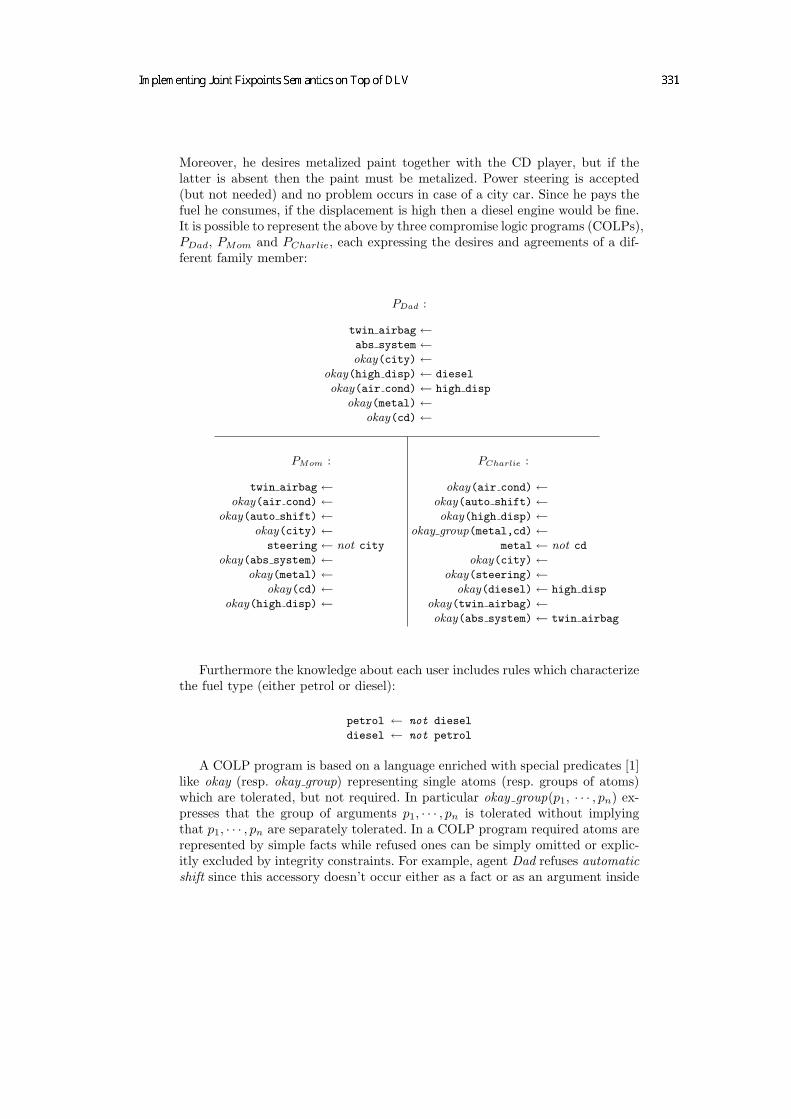
2

Moreover, he desires metalized paint together with the CD player, but if thelatter is absent then the paint must be metalized. Power steering is accepted(but not needed) and no problem occurs in case of a city car. Since he pays thefuel he consumes, if the displacement is high then a diesel engine would be fine.It is possible to represent the above by three compromise logic programs (COLPs),PDad, PMom and PCharlie, each expressing the desires and agreements of a dif-ferent family member:

PDad :

twin airbag ←abs system ←okay(city) ←

okay(high disp) ← diesel

okay(air cond) ← high disp

okay(metal) ←okay(cd) ←

PMom :

twin airbag ←okay(air cond) ←

okay(auto shift) ←okay(city) ←

steering ← not city

okay(abs system) ←okay(metal) ←

okay(cd) ←okay(high disp) ←

PCharlie :

okay(air cond) ←okay(auto shift) ←okay(high disp) ←

okay group(metal,cd) ←metal ← not cd

okay(city) ←okay(steering) ←

okay(diesel) ← high disp

okay(twin airbag) ←okay(abs system) ← twin airbag

Furthermore the knowledge about each user includes rules which characterizethe fuel type (either petrol or diesel):

petrol ← not diesel

diesel ← not petrol

A COLP program is based on a language enriched with special predicates [1]like okay (resp. okay group) representing single atoms (resp. groups of atoms)which are tolerated, but not required. In particular okay group(p1, · · · , pn) ex-presses that the group of arguments p1, · · · , pn is tolerated without implyingthat p1, · · · , pn are separately tolerated. In a COLP program required atoms arerepresented by simple facts while refused ones can be simply omitted or explic-itly excluded by integrity constraints. For example, agent Dad refuses automaticshift since this accessory doesn’t occur either as a fact or as an argument inside

3

an okay predicate, however this refuse could be also expressed by the rule:

⊥ ← auto shift

With regard to the example a common agreement will be reached on any ofthe following JFPs:

abs system, twin airbag, cd, city, metal, petrolabs system, twin airbag, air cond, cd, city, diesel, high disp, metalabs system, twin airbag, cd, city, diesel, metalabs system, twin airbag, cd, city, diesel, high disp, metalabs system, twin airbag, city, metal, petrolabs system, twin airbag, air cond, city, diesel, high disp, metalabs system, twin airbag, city, diesel, high disp, metalabs system, twin airbag, city, diesel, metal

Thus, each joint fixpoint represents a possible choice which is accepted byall the agents. Further constraints could be added in order to meet a particulartarget, e.g. when the car price is expressed as a function of the number and typeof chosen accessories and the agents have an upper bound on the money they canpay some of the above fixpoints may be rejected. However we do not consider thispossibility in this paper, leaving it as a matter for future work. An interestingcase is when agents’ default desire is saving money. Here minimal joint fixpointscan be adopted as a solution since they include only the minimum number ofatoms on which there is a common agreement. With regard to the example, theMJFPs characterizing the (possibly) cheapest cars are the following:

abs system, twin airbag, city, metal, petrolabs system, twin airbag, city, diesel, metal

In this work we present a framework which is able to compute either JFPsor MJFPs given an arbitrary set of COLP programs. In particular we performthe translation from COLP programs to classic logic programs and implementthe mapping from JFP semantics to SM semantics proposed in [1] in such away that a single classic logic program is generated whose stable models are inone-to-one correspondence with the JFPs. Moreover our framework enhances theabove mapping in order to work with non propositional programs and includesa wrapper exploiting the DLV system to compute the stable models. Finally, wecompute the minimal joint fixpoints as a further option.

The rest of the paper is structured as follows: in the next section we givea brief description of JFP semantics and then we consider the mapping fromJFP semantics to SM semantics. In Section 3 we describe in detail the sequenceof operations implementing the mapping and the algorithms exploited by theframework software modules. Moreover we consider some implementation issues.Finally, we draw in Section 4 our conclusions by considering possible alternativesolutions to the mentioned problems and proposing some optimizations to theframework.

4

2 The Joint Fixpoint Semantics

Before introducing JFP semantics, we briefly recall some basic concepts aboutlogic programming [2, 3] and stable models [5, 6]. Further details about JFPsemantics can be found in [1].

2.1 Basic Definitions

A term is either a variable or a constant. Variables are denoted by strings start-ing with uppercase letters, while those starting with lower case letters denoteconstants. An atom or positive literal is an expression p(t1, · · · , tn), where p is apredicate of arity n and t1, · · · , tn are terms. A negative literal is the negation asfailure (NAF) not a of a given atom a. A clause or rule r is a formula

a ← b1∧ · · · ∧bk∧not bk+1∧ · · · ∧not bm m ≥ 0.

where a, b1, · · · , bk are positive literals and not bk+1, · · · , not bm are negative lit-erals. a is called the head of r, while the conjunction b1∧ · · · ∧bk∧not bk+1∧· · · ∧not bm is the body of r. When m = 0 the rule r is said a fact, while if a = ⊥then r is said an integrity constraint.

A logic program is a finite set of rules. A term (an atom, a rule, a program,etc.) is called ground, if no variable appears in it. A ground program is also calleda propositional program.

Let V ar(P) be a finite set of atoms. A propositional logic program P definedon V ar(P) consists of a finite set of rules whose atoms are all in V ar(P).

A logic program is positive if no negative literal occurs in it.An (Herbrand) interpretation for a program P is a subset of V ar(P). A

positive literal a (resp. a negative literal not a) is true w.r.t. an interpretation Iif a ∈ I (resp. a /∈ I); otherwise it is false. A rule is satisfied (or is true) w.r.t. Iif its head is true or its body is false w.r.t. I. An interpretation I is a (Herbrand)model of a program P if it satisfies all rules in P.

For each program P, the immediate consequence operator TP is a functionfrom 2V ar(P) to 2V ar(P) defined as follows. For each interpretation I ⊆ V ar(P),TP(I) consists of the set of all heads of rules in P whose bodies evaluate to truein I.

An interpretation I is a fixpoint of a logic program P if I is a fixpoint of theassociated transformation TP , i.e., if TP(I) = I. The set of all fixpoints of P isdenoted by FP (P).

Let I be an interpretation of P and let a ∈ V ar(P) be an atom. We say that ais supported by I (in P) if there is a rule of P with head a whose body evaluatesto true in I, i.e., if a ∈ TP(I). From the definition of fixpoint it immediatelyfollows that an interpretation I of P is a fixpoint of P iff I coincides with theset of all atoms supported by I.

For any interpretation I ⊆ V ar(P), we define T 0P(I) = I and for all i ≥ 0,

T i+1P (I) = TP(T i

P(I)). If P is a positive program, then TP is monotonic and thushas a least fixpoint lfp(P) = T∞P (∅). This least fixpoint coincides with the least

5

Herbrand model lm(P) of P, i.e. lm(P) = lfp(P). For non-positive programs P,TP isn’t in general monotonic, and P does not necessarily have a least fixpoint(it may even have no fixpoint at all).

2.2 Stable Models

Let P be a logic program and I ⊆ V ar(P) be an interpretation. The Gelfond-Lifschitz transformation (or simply GL-transformation) of P w.r.t. I, denotedby PI is the program obtained by P by removing all rules containing a negativeliteral not b in the body such that b ∈ I, and by removing all negative literalsfrom the remaining rules.

Definition 1 ([5]). Given a logic program P and an interpretation M ⊆ V ar(P),M is a stable model of P if M = T∞PM (∅).

A logic program P admits in general a number (possibly zero) of stable models.We denote by SM(P) the set of all stable models of the program P.

2.3 Joint Fixpoints

In this section we recall the Joint Fixpoint Semantics for logic programs [1].Let S = P1,P2, · · · Pn be a set of logic programs such that V ar(P1) =

V ar(P2) = · · · = V ar(Pn) = V ar. We define the set JFP (P1,P2, · · · ,Pn) ofjoint fixpoints by:

JFP (P1,P2, · · · ,Pn) = FP (P1) ∩ FP (P2) ∩ · · · ∩ FP (Pn).

In words, JFP (P1,P2, · · · ,Pn) consists of all common fixpoints to the programsP1, · · · ,Pn.

Moreover, we define the set MJFP (P1, · · · ,Pn) of minimal joint fixpoint as:

MJFP (P1, · · · ,Pn) = F ∈ JFP (P1, · · · ,Pn) |6 ∃F ′ ∈ JFP (P1, · · · ,Pn) ∧ F ′ ⊂ F.

MJFP (P1, · · · ,Pn) consists of all minimal common fixpoints to the programsP1, · · · ,Pn.

2.4 Mapping Joint Fixpoints on Stable Models

In this section we briefly recall the translation from Logic Programming un-der the Joint Fixpoint Semantics to Logic Programming under Stable ModelSemantics. Further details can be found in [1].

Definition 2. Let P be a program and let M be a set of atoms in V ar(P). Wedenote by [M ]P the set aP | a ∈ M∪a′P | a ∈ V ar(P)\M∪saP | a ∈ M.

6

Here, with a little abuse of notation, aP , a′P and saP denote new atomsobtained through a sort of renaming operation performed on a, i.e. given anatom a, a new atom saP is created whose name is the same of a plus a prefix sand a suffix P .

Definition 3. Let P be a positive program. We define the program Γ (P) over theset of atoms V ar(Γ (P)) = aP | a ∈ V ar(P)∪a′P | a ∈ V ar(P)∪saP | a ∈V ar(P) ∪ failP as the union of the sets of rules S1, S2 and S3, defined asfollows:

S1 = aP ← not a′P | a ∈ V ar(P) ∪ a′P ← not aP | a ∈ V ar(P)

S2 = saP ← b1P , ..., bn

P | a ← b1, · · · bn ∈ PS3 = failP ← not failP , saP , not aP | a ∈ V ar(P)∪

failP ← not failP , aP , not saP | a ∈ V ar(P).The rules included in S1 guess potential fixpoints among the atoms which

are in V ar(P). Given an atom a ∈ V ar(P), aP represents a possible element ofa fixpoint of P, while a′P is its negated version so that only one of them can bepart of the same fixpoint. In S2 there are rules which characterize atoms whichare possibly included in stable models, and finally the rules in S3 state that anatom a is part of a fixpoint iff it is included in a stable model, i.e. fixpoints mustbe also stable models and vice-versa.

In [1] it was shown that a one-to-one correspondence exists between the setof fixpoints of a given program P and the set SM(Γ (P)) of stable models of theprogram Γ (P).

Now suppose we have a set of positive programs P1, · · · ,Pn over the same setof propositional variables. In [1] it was found a program J(P1, · · · ,Pn) associatedto the set of programs P1, · · · ,Pn such that the stable models of J(P1, · · · ,Pn)correspond to the joint fixpoints of P1, · · · ,Pn. J(P1, · · · ,Pn) is constructed byperforming the union of all the programs Γ (Pi), for 1 ≤ i ≤ n, with anotherprogram C(P1, · · · ,Pn) that we next define. Informally, under stable model se-mantics, rules of programs Γ (P1), Γ (P2), ... , Γ (Pn) have the effect of generatingall the fixpoints of P1, P2, ... , Pn, respectively, while rules of C(P1, · · · ,Pn) se-lect among these all fixpoints that are simultaneously fixpoints of P1, P2, ... ,Pn.

Definition 4. Given a set of positive programs P1, · · · ,Pn over the same set ofatomic propositions V ar, C(P1, · · · ,Pn) is the program over V ar′ =

⋃1≤i≤naPi

|a ∈ V ar ∪ fail defined as follows:

C(P1, · · · ,Pn) = fail ← not fail, aPi, not aPj

| 1 ≤ i 6= j ≤ n.

Moreover, the program J(P1, · · · ,Pn) over⋃

1≤i≤n V ar(Γ (Pi))∪fail is definedas:

J(P1, · · · ,Pn) = Γ (P1) ∪ · · · ∪ Γ (Pn) ∪ C(P1, · · · ,Pn).

7

The next theorem states that there is a one-to-one correspondence between theset of joint fixpoints of the programs P1, · · · ,Pn and the set of stable models ofthe program J(P1, · · · ,Pn).

Theorem 1. Let P1, · · · ,Pn be positive logic programs over the same set ofatomic propositions V ar. Then:

SM(J(P1, · · · ,Pn)) =⋃

F∈JFP (P1,...,Pn)

∪1≤i≤n[F ]Pi,

where JFP (P1, · · · ,Pn) is the set of the joint fixpoints of P1, · · · ,Pn.

2.5 Complexity Results

It was shown in [4] that it is NP complete to determine whether a single non-positive logic program has a fixpoint. The next table briefly introduces somedecision problems and describe their complexity. The reader may find furtherdetails in [1].

Problem Instance Question Complexity

JFP(JFP existence)

A set of positive logic programsP1, · · · ,Pn defined over thesame set of propositional vari-ables.

Is JFP (P1, · · · Pn) 6= ∅, i.e.,do the programs P1, · · · ,Pn

have a joint fixpoint?NP complete

MJFPs

(skeptical reasoningunder the JFP

semantics)

A set of positive logic programsS = P1, ...,Pn defined overthe same set of propositionalvariables V ar and an atomp ∈ V ar.

Does it hold that p ∈ I?For all the minimal joint fix-points I such thatI ∈ MJFP (P1, · · · ,Pn)

co-NP complete

MJFPc

(credulousreasoning under the

JFP semantics)

A set of positive logic programsS = P1, ...,Pn defined overthe same set V ar of proposi-tional variables and an atomp ∈ V ar.

Does it hold that p ∈ I?For some minimal joint fix-point I such thatI ∈ MJFP (P1, · · · ,Pn)

ΣP2 -complete

3 Framework Implementation

In this section we describe in detail the implementation of the framework.Our tool has a main front-end accepting in input a list of COLP programsand computing the joint fixpoints of such programs. This result is accomplishedthrough several stages as depicted in Figure 1.

In particular the overall process can be segmented into three big steps:

1. Converting a given set of COLP programs into classic propositional logicprograms.

2. Generating a single logic program whose stable models are in one-to-onecorrespondence with the joint fixpoints of the input COLP programs.

8

Fig. 1. JFP → SM mapping stages and software modules implemented

3. Exploiting the DLV system in order to compute the stable models of such aprogram and then computing the (minimal) joint fixpoints.

The first step is accomplished by the following two modules:

3.1 The Module colp2lp

Input: a list of non propositional COLP programs.Output: a list of non propositional classic logic programs.

This module translates a non propositional COLP program into a classic logicprogram, exploiting the conversion rules described in [1]. In particular all okayand okay group predicates are recognized and accordingly expanded into classicrules. Moreover each integrity constraint is mapped to a rule whose head atomdoesn’t occur in any other program. With regard to the beginning example, theCOLP PDad is translated into the following classic logic program:

twin airbag ←abs system ←

city ← city

high disp ← high disp, diesel

air cond ← air cond, high disp

metal ← metal

cd ← cd

As a further example, the statement okay group(metal,cd) included in theprogram PCharlie is converted into the following couple of rules:

metal ← metal, cd

cd ← metal, cd

9

3.2 The Module ground

Input: a list of non propositional classic logic programs.Output: a list of propositional classic logic programs.

The mapping proposed in [1] works only with propositional programs. As aconsequence, in order to give practical relevance to the implementation, we haveto deal with the non trivial issue of grounding. Observe that if we have in inputa set of non propositional COLP programs then the straight application of themapping presented in Section 2.4 may produce unsafe rules. A program rule issafe if each variable occurring in that rule appears in at least one positive literalin the body of the same rule [7, 8]: in particular the rules included in the setsS1, S3 and C are possibly unsafe because variables may occur as negative lit-erals inside the body of generated rules. Thus, for each input non propositionalprogram it is necessary to produce the corresponding propositional version. Byexploiting the tool Lparse [9–13] this module performs the required groundingon a given set of non propositional programs. However, a further issue has tobe considered: Lparse is optimized to discard those rules whose instantiationshave unsatisfiable bodies, i.e. when some literal in the body is not deducible.This kind of optimization is not applicable in case of the JFP semantics, whereokay and okay group predicates generate rules discarded by Lparse but mean-ingful w.r.t. the JFP semantics. Let us show the above issue by the example ofchat forum presented in [1]. In this example we have a chat forum involving afixed set of users: Ann, Bob, Connie and Dan. Each user can specify complexrequirements concerning the presence of other users in the forum. The followingCOLP program represents the requirements of the user Ann:

in forum(ann) ←okay(in forum(dan)) ←

okay group(in forum(bob),in forum(connie)) ← subject(soccer)

This program models the following specifications: Ann wants to enter in theforum and she tolerates the presence of Dan, but she does not require him.Moreover, the joint presence of Bob and Connie is tolerated, but only if socceris a subject of the forum.

The above okay and okay group predicates are translated as follows:

in forum(dan) ← in forum(dan)

in forum(bob) ← in forum(bob), in forum(connie), subject(soccer)

in forum(connie) ← in forum(bob), in forum(connie), subject(soccer)

Finally, the knowledge about each user is enriched by a common knowledgebase, defining the relationships user, day and subject. Furthermore the con-straint that a chat forum must contain at least two users is also included:

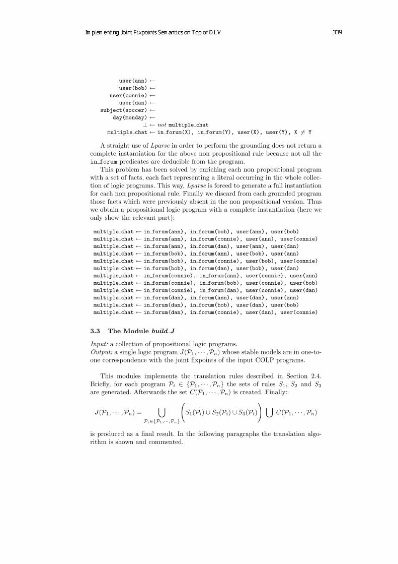
10

user(ann) ←user(bob) ←

user(connie) ←user(dan) ←

subject(soccer) ←day(monday) ←

⊥ ← not multiple chat

multiple chat ← in forum(X), in forum(Y), user(X), user(Y), X 6= Y

A straight use of Lparse in order to perform the grounding does not return acomplete instantiation for the above non propositional rule because not all thein forum predicates are deducible from the program.

This problem has been solved by enriching each non propositional programwith a set of facts, each fact representing a literal occurring in the whole collec-tion of logic programs. This way, Lparse is forced to generate a full instantiationfor each non propositional rule. Finally we discard from each grounded programthose facts which were previously absent in the non propositional version. Thuswe obtain a propositional logic program with a complete instantiation (here weonly show the relevant part):

multiple chat ← in forum(ann), in forum(bob), user(ann), user(bob)

multiple chat ← in forum(ann), in forum(connie), user(ann), user(connie)

multiple chat ← in forum(ann), in forum(dan), user(ann), user(dan)

multiple chat ← in forum(bob), in forum(ann), user(bob), user(ann)

multiple chat ← in forum(bob), in forum(connie), user(bob), user(connie)

multiple chat ← in forum(bob), in forum(dan), user(bob), user(dan)

multiple chat ← in forum(connie), in forum(ann), user(connie), user(ann)

multiple chat ← in forum(connie), in forum(bob), user(connie), user(bob)

multiple chat ← in forum(connie), in forum(dan), user(connie), user(dan)

multiple chat ← in forum(dan), in forum(ann), user(dan), user(ann)

multiple chat ← in forum(dan), in forum(bob), user(dan), user(bob)

multiple chat ← in forum(dan), in forum(connie), user(dan), user(connie)

3.3 The Module build J

Input: a collection of propositional logic programs.Output: a single logic program J(P1, · · · ,Pn) whose stable models are in one-to-one correspondence with the joint fixpoints of the input COLP programs.

This modules implements the translation rules described in Section 2.4.Briefly, for each program Pi ∈ P1, · · · ,Pn the sets of rules S1, S2 and S3

are generated. Afterwards the set C(P1, · · · ,Pn) is created. Finally:

J(P1, · · · ,Pn) =⋃

Pi∈P1,···,Pn

(S1(Pi) ∪ S2(Pi) ∪ S3(Pi)

) ⋃C(P1, · · · ,Pn)

is produced as a final result. In the following paragraphs the translation algo-rithm is shown and commented.

11

The Translation Algorithm

Algorithm TranslateInput V ar: Set of atoms, P = P1, · · · ,Pi, · · · ,Pn: Set of logic programs over V ar;Output J(P1, · · · ,Pn): a program associated to the set P such that the stable

models of J(P1, · · · ,Pn) correspond to the joint fixpoints of P1, · · · ,Pn;var S1, S2, S3, C, Γ (P1), · · · , Γ (Pi), · · · , Γ (Pn): Set of rules, LSet, L: List of atoms;begin1. for each integer i | ∃ a program Pi ∈ P do

(* S1 and S3 are created *)2. S1 = ∅; S2 = ∅; S3 = ∅;3. for each atom a ∈ V ar do4. let a1 be a new literal; a1.setName(a.getName + “p” + int2string(i));5. let a2 be a new literal; a2.setName(a.getName + “ ′ ” + “p” + int2string(i));6. let r be a new rule; r.setHead([a1.getName]); r.setBody([not a2.getName]);7. let s be a new rule; s.setHead([a2.getName]); s.setBody([not a1.getName]);8. S1 = S1 ∪ r ∪ s;9. let a3 be a new literal; a3.setName(“s” + a.getName + “p” + int2string(i));

10. let a4 be a new literal; a4.setName(“fail” + “p” + int2string(i));11. let t be a new rule; t.setHead([a4.getName]);12. t.setBody([not a4.getName, a3.getName, not a1.getName]);13. let u be a new rule; u.setHead([a4.getName]);14. u.setBody([not a4.getName, a1.getName, not a3.getName]);15. S3 = S3 ∪ t ∪ u;16. end for

(* S2 is created*)17. for each rule r ∈ Pi | r : a ← b1, · · · , bn do18. let l be a new literal; l.setName(“s” + a.getName + “p” + int2string(i));19. LSet = ∅;20. for each bj ∈ Body(r)21. let lj be a new literal; lj .setName(bj .getName + “p” + int2string(i));22. let LSet = LSet ∪ lj;23. end for24. let L = SetToList(LSet);25. let s be a new rule; s.setHead([l.getName]); s.setBody(L);26. S2 = S2 ∪ s;27. end for

(* Γ (Pi) is created*)28. Γ (Pi) = S1 ∪ S2 ∪ S3;29. end for

(* C(P1, · · · ,Pn) is created *)30. C = ∅;31. let f be a new literal; f.setName(“fail”);32. for each atom a ∈ V ar do33. for each integer i ∈ [1, n] do34. let aPi

be a new literal; aPi.setName(a.getName + “p” + int2string(i));

35. for each integer j ∈ [1, n] do36. if i 6= j then37. let aPj

be a new literal; aPj.setName(a.getName + “p” + int2string(j));

38. let r be a new rule; r.setHead([f.getName]);39. r.setBody([not f.getName, aPi

.getName, not aPj.getName]);

40. C = C ∪ r;41. end if42. end for43. end for44. end for

(* J(P1, · · · ,Pn) is created *)45. J = ∅;46. for each integer i ∈ [1, n] do47. J = J ∪ Γ (Pi);48. end for49. J = J ∪ C;end.

12

Comments to the Algorithm

W.l.o.g. we assume the logic programs P1, · · · ,Pn being defined over the sameset V ar. Furthermore we assume V ar being part of the input. A more generalscenario has been implemented where each logic program can be defined on adifferent set of atoms V ar(Pi) not being part of the input, but built at run-time.Moreover the set V ar is generated as the union of all the sets V ar(Pi).

lines 2 - 8: For each program Pi these statements build the set S1:lines 2 - 5: For each atom a ∈ V ar two literals aPi and a′Pi

are created.Atoms and literals are treated as objects having an attribute name. Weassume that two methods getName and setName exist which are usedto read / write such attribute. The function int2string returns the stringrepresentation of an integer number.

lines 6 - 8: For each atom a ∈ V ar two rules aPi ← not a′Piand a′Pi

←not aPi are created. Rules are treated as objects having two attributes:a Head and a Body. The method setHead (resp. setBody) receives a listL = [l1, · · · , ln] of literals and sets the head (resp. the body) of a specifiedrule using the literals inside L. After being created the rules are addedto the set S1.

lines 9 - 16: For each program Pi these statements build the set S3:lines 9 - 10: For each atom a ∈ V ar two literals saPi

and failPiare cre-

ated.lines 11 - 16: For each atom a ∈ V ar two rules failPi

← not failPi, saPi

,not aPi

and failPi← not failPi

, aPi, not saPi

are created. Finally thoserules are added to the set S3.

lines 17 - 27: For each program Pi, the set S2 is created. In particular:lines 18 - 23: Each rule r of the form: a ← b1, · · · , bn is renamed to a new

rule s : saPi← b1

Pi, · · · , bn

Pi. A set LSet is used to temporarily store the

literals from the body of s.lines 24 - 27: The set LSet is converted to a list L which is input to the

method setBody. Then the rule s is added to the set S2.line 28: For each program Pi a new program Γ (Pi) = S1 ∪ S2 ∪ S3 is created.lines 30 - 44: The set C = C(P1, · · · ,Pn) is created. In particular for each

atom a ∈ V ar and for each couple of different programs Pi and Pj twonew literals aPi , aPj and a rule of the form fail ← not fail, aPi , not aPj arecreated. Then those rules are added to C.

lines 45 - 49: J(P1, · · · ,Pn) is created as J = Γ (P1) ∪ · · · ∪ Γ (Pn) ∪ C.

At this stage we exploit the DLV system [7, 8] in order to compute the stablemodels of J(P1, · · · ,Pn).

3.4 The Module parse SM

Input: the stable models of the program J(P1, · · · ,Pn).Output: the joint fixpoints of P1, · · · ,Pn.

13

This module post-processes the output results from DLV. In particular itfilters the stable models of J(P1, · · · ,Pn) extracting the relevant atoms, i.e. thosebeing part of JFP(P1, · · · ,Pn). Finally the original names those atoms had withinthe COLP programs are restored, i.e. name prefixes and suffixes added by thetranslation process are discarded. For example, a stable model of J(P1, · · · ,Pn)is the following:s abs system P1, s twin airbag P1, s twin airbag P2, abs system P1,

air cond 1 P1, cd P1, city P1, diesel 1 P1, high disp 1 P1, metal P1,

petrol P1, twin airbag P1, s cd P1, s city P1, s metal P1, s petrol P1,

abs system P2, air cond 1 P2, auto shift 1 P2, cd P2, city P2, diesel 1 P2,

high disp 1 P2, metal P2, petrol P2, steering 1 P2, twin airbag P2,

s abs system P2, s cd P2, s city P2, s metal P2, s petrol P2, abs system P3,

air cond 1 P3, auto shift 1 P3, cd P3, city P3, diesel 1 P3, high disp 1 P3,

metal P3, petrol P3, steering 1 P3, twin airbag P3, s abs system P3, s cd P3,

s city P3, s metal P3, s petrol P3, s twin airbag P3where all atoms having a prefix s (the supported atoms) jointly occur with

those without the prefix (the fixpoints) as an effect of the rules in S3. Moreoverthe suffix Pi indicates which logic program an atom comes from.

From this stable model the following joint fixpoint is extracted:abs system, twin airbag, cd, city, metal, petrol

3.5 The Module find MJFP

Input: the joint fixpoints of P1, · · · ,Pn.Output: the minimal joint fixpoints of P1, · · · ,Pn.

The set of minimal joint fixpoints MJFP(P1, · · · ,Pn) is built in a bottom-upfashion. At the beginning MJFP is empty and the input joint fixpoints are sortedby ascending cardinality, i.e. the number of included atoms. Fixpoints having theminimum cardinality are also minimal, thus they are directly included in MJFP.The remaining fixpoints are separately processed: a fixpoint is discarded if anelement of MJFP exists which is included in it, otherwise it is added to MJFP.In the following paragraphs the algorithm is shown and commented.

3.6 MJFP Search Algorithm

Algorithm MJFP SearchInput JFP (P1, · · · ,Pn): Set of joint fixpoints of the programs P1, · · · ,Pn.Output MJFP (P1, · · · ,Pn): Set of minimal joint fixpoints of the programs P1, · · · ,Pn.var L: List of fixpoints; mincard: Integer; discard: Boolean;begin1. for each element f ∈ JFP (P1, · · · ,Pn) do2. L.append(f);3. end for4. sort(L, cardinality, ascending);5. mincard = card(L.first); MJFP = ∅;6. for each element l in list L do7. if card(l) = mincard then MJFP = MJFP ∪ l;8. else begin

14

9. discard = false;10. for each element m ∈ MJFP do11. if m ⊆ l then discard = true;12. end for13. if not discard then MJFP = MJFP ∪ l;14. end;15. end forend.

Comments to the Algorithm

lines 1 - 3: The elements of JFP (P1, · · · ,Pn) are copied in a list L.line 4: The elements of L are sorted by ascending cardinalities, i.e. number of

included atoms.lines 6 - 15: This is the core of the algorithm, in particular:

line 7: Fixpoints having the minimum cardinality are added to MJFP.lines 8 - 12: Fixpoints not having the minimum cardinality are checked

for set inclusion minimality: if any of them includes an element of MJFPthen it is discarded.

lines 13 - 15: Fixpoints which are not discarded are minimal, so they areadded to MJFP.

Furthermore, even though the algorithm works in polynomial time, spacecomplexity represents a concrete drawback. In fact all joint fixpoints have to becomputed before finding the minimal ones, i.e. exponential space is required. Asdiscussed in the next section, an interesting issue to be investigated is of coursethe problem of encoding minimality directly into the original programs in orderto avoid space exploitation generated by the previous approach. However, thisapproach may have significance every time the number of JFPs is small, that is aplausible case, since it corresponds to have heterogeneous agents’ requirements.

4 Conclusions and Future Work

In this paper we described a framework which implements the joint fixpointsemantics introduced in [1] on the top of the DLV system. This semantics issuitable to model joint decisions of agents represented by logic programs. Inorder to meet this target we realized software tools which receive in input a col-lection of COLP programs, each representing the requirements and desires of anagent, and generate a single program whose stable models are in one-to-one cor-respondence to the COLPs’ joint fixpoints. Those stable models are computedexploiting the DLV system. As a final result we compute the joint fixpoints ofthe input COLP programs, i.e. the fixpoints which are common to all the inputCOLP programs. Those joint fixpoints represent a common agreement amongthe agents. Moreover we embedded an option to compute the minimal joint fix-points, i.e. the joint fixpoints containing the minimum number of atoms requiredto meet a common agreement between the agents. It is easy to see that the com-putational complexity of the implementation reaches the theoretic one. It has

15

been pointed out that searching for the minimal joint fixpoints requires an expo-nential space, thus a new scheme for the mapping from joint fixpoint semanticsto stable model semantics has to be investigated in order to directly produce theminimal joint fixpoints. Grounding is another issue that could be solved in analternative way: again, by changing the translation scheme it could be possibleto avoid the generation of unsafe rules within the sets S1, S3 and C. This way thetranslation process could directly work with non propositional COLP programs,thus avoiding the overhead produced by the ground instantiations. This is leftfor future investigations.

References

1. Buccafurri, F., Gottlob, G.: Multiagent Compromises, Joint Fixpoints and StableModels. Computational Logic: From Logic Programming into the Future (In honourof Bob Kowalsky), Ed. A. Kakas and F. Sadri, Springer Verlag (2002)

2. Baral C., Gelfond M.: Logic Programming and Knowledge Representation. Journalof Logic Programming 19-20, (1994) 73–148

3. Minker J., Seipel D.: Disjunctive Logic Programming: A Survey and Assessment.Computational Logic: From Logic Programming into the Future (In honour of BobKowalsky), Ed. A. Kakas and F. Sadri, Springer Verlag (2002)

4. Kolaitis, P.G., Papadimitriou, C.H.: Why not Negation by Fixpoint? Journal ofComputer and System Sciences 43(1), (1991) 125–144

5. Gelfond, M., Lifschitz, V.: The Stable Model Semantics for Logic Programming.Proceedings of the 5th International Conference on Logic Programming, MIT Press,Cambridge, (1988) 1070–1080

6. Baral C.: Knowledge Representation, Reasoning and Declarative Problem Solving.Cambridge University Press, (2003)

7. Leone, N., Pfeifer, G., Faber, W., Calimeri, F., Dell’Armi, T., Eiter, T, Gottlob,G., Ianni, G., Ielpa, G., Koch, C., Perri, S., and Polleres, A.: The DLV System.Proceedings of the 8th European Conference on Logics in Artificial Intelligence(JELIA) n.2424 in Lecture Notes in Computer Science, (2002) 537–540

8. Bihlmeyer, R., Faber, W., Ielpa, G., and Pfeifer, G.: DLV - User Manual.Available at: http://www.dlvsystem.com

9. Syrjanen, T.: Lparse 1.0 User’s Manual.Available at: http://www.tcs.hut.fi/Software/smodels/lparse.ps.gz

10. Niemela, I., Simons, P.: Smodels - an Implementation of the Stable Model and Well-founded Semantics for Normal Logic Programs. Proceedings of the 4th InternationalConference on Logic Programming and Non-Monotonic Reasoning (LPNMR ’97),Lecture Notes in Computer Science, Vol. 1265. Springer-Verlag, Dagstuhl, Ger-many (1997) 420–429

11. Niemela, I., Simons, P., and Syrjanen, T.: Smodels: a system for answer set pro-gramming. Proceedings of the 8th International Workshop on Non-Monotonic Rea-soning, Breckenridge, Colorado, USA, (2000)

12. Syrjanen, T.: Implementation of Local Grounding for Logic Programs with Sta-ble Model Semantics. Technical Report, Helsinki University of Technology, DigitalSystems Laboratory, (1998)

13. Simons, P.,Niemela, I.,and Soinen, T.: Extending and Implementing the stablemodel semantics. Artificial Intelligence 138, (2002)

A compositional Semantics for CHR

Maurizio Gabbrielli and Maria Chiara Meo

Dipartimento di Scienze dell’Informazione, Universita di Bologna,Mura A.Zamboni 7, 40127 Bologna, Italy

gabbri@cs.unibo.it Dipartimento di Scienze, Universita di Chieti

Viale Pindaro 42, 65127 Pescara, Italycmeo@unich.it

Abstract.Constraint Handling Rules (CHR) is a committed-choice declarative languagewhich has been designed for writing constraint solvers. A CHR program consistsof multi-headed guarded rules which allow to rewrite constraints into simplerones until a solved form is reached.CHR has received a considerable attention, both from the practical and from thetheoretical side. Nevertheless, due the use of multi-headed clauses, there are sev-eral aspects of the CHR semantics which are not been clarified yet. In particular,no compositional semantics for CHR has been defined so far.In this paper we introduce a fix-point semantics which characterizes the input/outputbehavior of a CHR program and which is and-compositional, that is, which al-lows to retrieve the semantics of a conjunctive query from the semantics of itscomponents. Such a semantics can be used as a basis to define incremental andmodular analysis and verification tools.

1 Introduction

Constraint Handling Rules (CHR) [9, 10] is a committed-choice declarative languagewhich has been specifically designed for writing constraint solvers. The first constraintlogic languages used mainly built-in constraint solvers designed by following a “blackbox” approach. This made hard to modify, debug, and analyze a specific solver. More-over, it was very difficult to adapt an existing solver to the needs of some specific ap-plications, and this was soon recognized as a serious limitation since often practicalapplications involve application specific constraints.

By using CHR one can easily introduce specific user-defined constraints and therelated solver into an host language. In fact, a CHR program consists of (a set of) multi-headed guarded simplification and propagation rules which are specifically designed toimplement the two most important operations involved in the constraint solving pro-cess: Simplification rules allow to replace constraints by simpler ones, while preservingtheir meaning. Propagation rules are used to add new redundant constraints which donot modify the meaning of the given constraint and which can be useful for further re-ductions. It is worth noting that the presence of multiple heads in CHR is an essentialfeature which is needed in order to define reasonably expressive constraint solvers (seethe discussion in [10]). However, such a feature, which differentiates this proposal from

2

many existing committed choice logic languages, complicates considerably the seman-tics of CHR, in particular it makes very difficult to obtain a compositional semantics, aswe argue below. This is unfortunate, as compositionality is an highly desirable propertyfor a semantics. In fact, a compositional semantics provides the basis to define incre-mental and modular tools for software analysis and verification, and these features areessential in order to deal with partially defined components. Moreover, in some cases,modularity allows to reduce the complexity of verification of large systems by consid-ering separately smaller components.

In this paper we introduce a fix-point semantics for CHR which characterizes the in-put/output behavior of a program and which is and-compositional, that is, which allowsto retrieve the semantics of a conjunctive query from the semantics of its components.

In general, due to the presence of synchronization mechanisms, the input/ouputsemantics is not compositional for committed choice logic languages and for most con-current languages in general. Indeed, the need of more complicate semantic structuresbased on traces was recognized very early as a necessary condition to obtain a com-positional model, first for dataflow languages [11] and then in the case of many otherparadigms, including imperative concurrent languages [7] and concurrent constraint andlogic languages [5].

When considering CHR this basic problem is further complicated: due to the pres-ence of multiple heads the traces consisting of sequences of input/ouput pairs, analo-gous to those used in the above mentioned works, are not sufficient to obtain a com-positional semantics. Intuitively the problem can be stated as follows. A CHR rule cannot be used to rewrite a goal , no matter how the variablesare constrained (that is, for any input constraint), because the goal consists of a singleatom while the head of the rule contains two atoms . Therefore, if we considereda semantics based on input/ouput traces, we would obtain the empty denotation for thegoal in the program consisting of the rule plus some rules defining . Analogouslyfor the goal . On the other hand, the rule can be used to rewrite the goal .Therefore, provided that the semantics of is not empty, the semantics of is notempty and cannot be derived from the semantics of and , that is, such a semanticsis not compositional. It is worth noting that even restricting to a more simple notionof observable, such as the results of terminating computations, does not simplify thisproblem. In fact, differently from the case of ccp languages, also the semantic based onthese observables (usually called resting points) is not compositional for CHR.

Our solution to obtain a compositional model is to use an augmented semanticsbased on traces which includes at each steps two “assumptions” on the external envi-ronment and two “outputs” of the current process: Similarly to the case of the modelsfor ccp, the first assumption is made on the constraints appearing in the guards of therules, in order to ensure that these are satisfied and the computation can proceed. Thesecond assumption is specific to our approach and contains atoms which can appear inthe heads of rules. This allows us to rewrite a goal by using a rule whose head

properly contains : While this is not possible with the standard CHR semantics, weallow that by assuming that the external environment provides the “difference” mi-nus and by memorizing such an assumption. The first output element is the constraintproduced by the process, as usual. We also memorize at each step also a second output

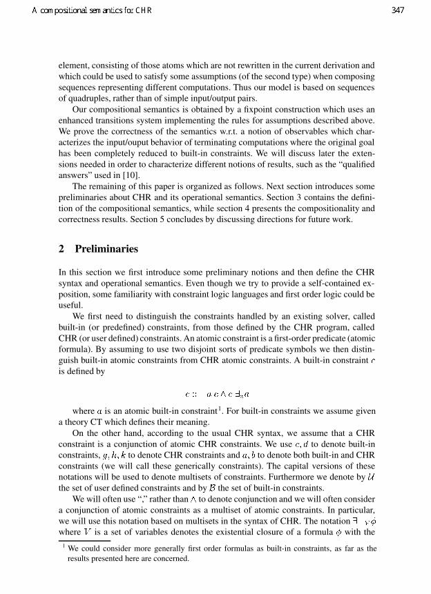
3

element, consisting of those atoms which are not rewritten in the current derivation andwhich could be used to satisfy some assumptions (of the second type) when composingsequences representing different computations. Thus our model is based on sequencesof quadruples, rather than of simple input/output pairs.

Our compositional semantics is obtained by a fixpoint construction which uses anenhanced transitions system implementing the rules for assumptions described above.We prove the correctness of the semantics w.r.t. a notion of observables which char-acterizes the input/ouput behavior of terminating computations where the original goalhas been completely reduced to built-in constraints. We will discuss later the exten-sions needed in order to characterize different notions of results, such as the “qualifiedanswers” used in [10].

The remaining of this paper is organized as follows. Next section introduces somepreliminaries about CHR and its operational semantics. Section 3 contains the defini-tion of the compositional semantics, while section 4 presents the compositionality andcorrectness results. Section 5 concludes by discussing directions for future work.

2 Preliminaries

In this section we first introduce some preliminary notions and then define the CHRsyntax and operational semantics. Even though we try to provide a self-contained ex-position, some familiarity with constraint logic languages and first order logic could beuseful.

We first need to distinguish the constraints handled by an existing solver, calledbuilt-in (or predefined) constraints, from those defined by the CHR program, calledCHR (or user defined) constraints. An atomic constraint is a first-order predicate (atomicformula). By assuming to use two disjoint sorts of predicate symbols we then distin-guish built-in atomic constraints from CHR atomic constraints. A built-in constraint is defined by

where is an atomic built-in constraint1. For built-in constraints we assume givena theory CT which defines their meaning.

On the other hand, according to the usual CHR syntax, we assume that a CHRconstraint is a conjunction of atomic CHR constraints. We use to denote built-inconstraints, to denote CHR constraints and to denote both built-in and CHRconstraints (we will call these generically constraints). The capital versions of thesenotations will be used to denote multisets of constraints. Furthermore we denote by the set of user defined constraints and by the set of built-in constraints.

We will often use “,” rather than to denote conjunction and we will often considera conjunction of atomic constraints as a multiset of atomic constraints. In particular,we will use this notation based on multisets in the syntax of CHR. The notation

where is a set of variables denotes the existential closure of a formula with the1 We could consider more generally first order formulas as built-in constraints, as far as the

results presented here are concerned.

4

exception of the variables which remain unquantified. denotes the free vari-ables appearing in and we denote by the concatenation of sequences and by theempty sequence. Furthermore denotes the multi-set union, while we consider as anoverloaded operator used both for set and multi-set difference (the meaning depends onthe type of the arguments).

We are now ready to define the CHR syntax.

Definition 1 (Syntax). [10] A CHR simplification rule has the form whilea CHR propagation rule has the form where is a non-empty multiset ofuser-defined constraints, is a built-in constraint and is a possibly empty multi-setof constraints.

A CHR program is a set of CHR simplification and propagation rules. A CHR goalis a multiset of (both user defined an built-in) constraints.

We prefer to use multisets rather than sequences (as in the original CHR papers)since multisets appear to correspond more precisely to the nature of CHR rules. Wedenote by the set of all goals.

We describe now the operational semantics of CHR as provided by [10] by using atransition system ( here stands for “standard”, as opposed to thesemantics we will use later). Configurations in are triples of the form where are the constraints that remain to be solved, are the user-defined constraintsthat have been accumulated and are the built-in constraints that have been simplified 2.

An initial configuration has the form

and consists of a query , an empty user-defined constraint and an empty built-in con-straint.

A final configuration has either the form

when it is failed, i.e. when it contains an inconsistent built-in constraint store repre-sented by the unsatisfiable constraint false, or has the form

when it is successfully terminated, i.e. there are no goals left to solve.Given a program , the transition relation is the least relation

satisfying the rules in Table 1 (for the sake of simplicity, we omit indexing the relationwith the name of the program). The Solve transition allows to update the constraintstore by taking into account a built-in constraint contained in the goal. Without loss ofgenerality, we will assume that . The Introduce transition is

2 In [10] triples of the form were used, where the annotation , which is not changedby the transition rules, is used to distinguish the variables appearing in the initial goal fromthe variables which are introduced by the rules. We can avoid such an indexing by explicitlyreferring to the original goal.

5

Solve and c is a built-in constraint

Introduce h is a user-defined constraint

Simplify

Propagate

Table 1. The standard transition system for CHR

used to move a CHR constraint from the goal to the CHR constraint store, where it canbe handled by applying CHR rules. The transitions Simplify and Propagate allow torewrite CHR constraints (which are in the CHR constraint store) by using rules fromthe program. As usual, in order to avoid variable names clashes, both these transitionsassume that clauses from the program are renamed apart, that is assume that all vari-ables appearing in a program clause are fresh ones. Both the Simplify and Propagatetransitions are applicable when the current store () is strong enough to entail the guardof the rule (), once the parameter passing has been performed (this is expressed by theequation ). Note that, due to the existential quantification over the variables appearing in , in such a parameter passing the information flow is from the actualparameter (in ) to the formal parameters (), that is, it is required that the constraints which have to be rewritten are an instance of the head . When applied, both thesetransitions add the body of the rule to the current goal and the equation ,expressing the parameter passing mechanism, to the built-in constraint store. The dif-ference between Simplify and Propagate is in the fact that while the former transitionremoves the constraints which have been rewritten from the CHR constraint store,this is not the case for the latter.

Given a goal , the operational semantics that we consider observes the final storesof computations terminating with an empty goal and an empty user-defined constraint.We call these observables success answers slightly deviating from the terminology of[10] (a goal which has a success answer is called a data-sufficient goal in [10]).

Definition 2 (Success answers). Let be a program and let be a goal. The set of success answers for the query in the program is defined as follows

In [10] it is considered also the following different notion of answer, obtained bycomputations terminating with a user-defined constraint which does not need to beempty.

6

Definition 3 (Qualified answers). Let be a program and let be a goal. The set of qualified answers for the query in the program is defined as follows

We discuss in Section 5 the extensions needed to characterize also qualified answers.Note that both previous notions of observables characterize an input/output behavior,since the input constraint is implicitly considered in the goal.

In the remaining of this paper we will consider only simplification rules since prop-agation rules can be mimicked by simplification rules, as far as the results contained inthis paper are concerned.

3 A compositional trace semantics

Given a program , we say that a semantics is and-compositional if for a suitable composition operator which does not depend on theprogram . As mentioned in the introduction, due to the presence of multiple headsin CHR, the semantics which associate to a program the function is not and-compositional, since goals which have the same input/ouput behavior can behave differ-ently when composed with other goals. Consider for example the program consistingof the single rule

(where is a built-in constraint). According to Definition 3 we have that , while . An analogousexample can be made to show that also the semantics is not and-compositional.

The problem exemplified above is different from the classic problem of concur-rent languages where the interaction of non-determinism and synchronization makesthe input/outuput observables non-compositional. For this reason, considering simplysequences of (input-output) built-in constraints is not sufficient to obtain a composi-tional semantics for CHR. We have to use some additional information which allow usto describe the behavior of goals in any possible and-composition without, of course,considering explicitly all the possible and-compositions.

The basic idea of our approach is to collect in the semantics also the “missing”parts of heads which are needed in order to proceed with the computation. For example,when considering the program above, we should be able to state that the goal

produces the constraint , provided that the external environment (i.e. a conjunctivegoal) contains the CHR constraint . In other words, is an assumption which is madein the semantics describing the computation of . When composing (by using a suitablenotion of composition) such a semantics with that one of a goal which contains wecan verify that the “assumption” is satisfied and therefore obtain the correct semanticsfor . In order to model correctly the interaction of different processes we have to usesequences, analogously to what happens with other concurrent paradigms.

This idea is developed in the following by defining a new transition system whichimplements this mechanism based on assumptions for dealing with the missing partsof heads. The new transition system allows to generate the sequences appearing in the

7

Solve’

Simplify’

Table 2. The transition system for the compositional semantics

compositional model by using a standard fix-point construction. As a first step in ourconstruction we modify the notion of configuration used before: Since we do not needto distinguish user defined constraints which appear in the goal from the user definedconstraints which have been already considered for reduction, we merge the first andthe second components of previous triples. On the other hand, we need the informationon the new assumptions, which is added as a label of the transitions.

Thus we define a transition system where configurations inConf are pairs: the first component is a multi-set of indexed atoms (the goal) andthe second one is a built-in constraint (the store). Indexes are associated to atoms inorder to denote the point in the derivation where they have been introduced. Moreprecisely, atoms in the original goals are labeled by , while atoms introduced at the derivation step are labeled by . Given a program , the transition relation is the least relation satisfying the rules in Table 2.Note that we consider only Solve and Simplify rules, as the other rules as previouslymentioned are redundant in this context. Solve’ is the same rule as before, while theSimplify’ rule is modified to consider assumptions: When reducing a goal by usinga rule having head , the set of assumption (with ) is used tolabel the transition ( here denotes multiset difference). Indexes allow us to distinguishidentical occurrences of atoms which have been introduced in different derivation steps.We will use the notation to indicate that is the maximal label occurring in the(non-atomic) goal and to indicate that all the atoms in are labeled by . When noambiguity arise, to simplify the notation we will use also to denote . In par-ticular, the notation used in some cases in the transitions alwaysmeans , that is, if is the maximal label occurring in thenall the atoms in are labeled by . When indexes are not needed we will simplyomit them. As before, we assume that program rules to be used in the new simplify ruleuse fresh variables to avoid names captures.

The semantics domain of our compositional semantics is based on sequences whichrepresent derivations obtained by the transition system in Table 2. More precisely, wefirst consider “concrete” sequences consisting of tuples of the form :Such a tuple represents exactly a derivation step . The sequenceswe consider are terminated by tuples of the form , which represent a termi-nating step (see the precise definition below). Since a sequence represents a derivation,we assume that the “output” goal at step is equal to the “input” goal at step ,

8

that is, we assume that if

appears in a sequence, then holds.

On the other hand, the input store can be different from the output store produced at previous step, since we need to perform all the possible assumptions on theconstraint produced by the external environment in order to obtain a compositionalsemantics. However, we assume that if

appears in a sequence then holds: This means that the assumptionmade on the external environment cannot be weaker than the constraint store producedat the previous step. This reflects the monotonic nature of computations, where infor-mation can be added to the constraint store and cannot be deleted from it. Finally notethat assumptions on CHR constraints (label ) are made only for the atoms which areneeded to “complete” the current goal in order to apply a clause. In other words, no as-sumption can be made in order to apply clauses whose heads do not share any predicatewith the current goal.

The set of the above described “concrete” sequences, which represent derivationsteps performed by using the new transition system, is denoted by .

From these concrete sequences we extract some more abstract sequences which arethe objects of our semantic domain: From each tuple in a sequenceÆ we extract a tuple of the form where we consider as before theinput and output store ( and , respectively) and the assumptions (), while we donot consider anymore the output goal . Furthermore, we restrict the input goal tothat part consisting of all those user-defined constraints which will not be rewrittenin the (derivation represented by the) sequence Æ. Intuitively contains those atomswhich are available for satisfying assumptions of other goals, when composing twodifferent sequences (representing two derivations of different goals). We also assumethat if is in a sequence then holds,since these atoms which will not be rewritten in the derivation can only augment. Wethen define formally the semantic domain as follows.

Definition 4 (Sequences). The semantic domain containing all the possible sequencesis defined as the set

for each ! ! " and for each " and are multisets of CHR indexed constraints, are built-in constraints such that

and

In order to define our semantics we need two more notions. First, we define anabstraction operator # which extracts from the concrete sequences in (representingexactly derivation steps) the sequences used in our semantic domain.

9

Definition 5. Let Æ be a sequence ofderivation steps where we assume that atoms are indexed as previously specified. Wesay that an indexed atom is stable in Æ if appears in and in , for each " . The abstraction operator # is then defined inductively as

#

# Æ #Æ

where is the multiset consisting of all the indexed atoms in which are stable in Æ.

Then we need the notion of “compatibility” of a tuple w.r.t. a sequence. To this aimwe first provide some further notation: Given a sequence of derivation steps

Æ

we denote by "Æ and by "Æ the length of the derivation Æ and the first in-put store , respectively. Moreover using as a shorthand for the tuple we define

,Æ ,Æ

,

Æ ,Æ

and

Æ .

We then define a compatibility as follows.

Definition 6. Let a tuple representing a derivation step forthe goal and let Æ be a sequence ofderivation steps for . We say that is compatible with Æ if the following hold:

1. "Æ ,2. Æ ,

3. for ", Æ and

4. Æ .

Note that if is compatible with Æ then, by using the notation above, Æ is a sequenceof derivation steps for . We can now define the compositional semantics.

Definition 7 (Compositional semantics). Let be a program and let be a goal. Thecompositional semantics of in the program , , is defined as

#

10

where # is the operator introduced in Definition 5 and is defined

as follows:

Æ and Æ for some Æ such that is compatible with Æ

Formally is defined as the least fixed-point of the corresponding operator$ defined by

$% Æ and Æ % for some Æ such that is compatible with Æ

In the above definition, the ordering on is that of (point-wiseextended) set-inclusion. It is straightforward to check that $ is continuous (on a CPO),thus standard results ensure that the fixpoint can be calculated by

, where is the identity map and for " & , = Æ (see for example [8]).

4 Compositionality and correctness

In this section we prove that the semantics defined above is and-compositional andcorrect w.r.t. the observables .

In order to prove the compositionality result we first need to define how two se-quences describing a computation of and , respectively, can be composed in orderto obtain a computation of . Such a composition is defined by the (semantic) oper-ator which performs an interleaving of the actions described by the two sequences andthen eliminates the assumptions which are satisfied in the resulting sequence. For tech-nical reasons, rather than modifying the existing sequences, the elimination of satisfiedassumptions is performed on new sequences which are generated by a closure operator' defined as follows.

Definition 8. Let ( be a multiset of indexed atoms and let ) be a sequence in of theform

We denote by ) ( the sequence

( (

where the multisets difference ( considers indexes.The operator ' is defined as follows. Given * , '* is the

least set satisfying the following conditions:

11

1. * '*;2. if ) ) * then ) ) ( '*

where is a multiset such that there exists a multiset (ofindexed atoms) (

such that , for each

".

A few explanations are in order. The operator ' is an upper closure operator 3 whichsaturates a set of sequences * by adding new sequences where redundant assumptionscan be removed: an assumptions (in ) can be removed if appears as a stableatom (in ). Once a stable atom is “consumed” for satisfying an assumption it isremoved from (the sets of stable atoms of) all the tuples appearing in the sequence, toavoid multiple uses of the same atom. Note that stable atoms are considered withoutthe index in the condition , while they are considered asindexed atoms in the removal operation ( . The reason for this slight complicationis explained by the following example. Assume that we have the set * consisting of theonly sequence . Such a sequence indicates that at thesecond step we have an assumption , while both at the first and at the second step wehave produced a stable atom , which has been indexed by and , respectively. In orderto satisfy the assumption we can use either or . However, depending on whatindexed atom we use, we obtain two different simplified sequences in '*, namely and , which describes correctlythe two different situations.

Before defining the composition operator on sequences we need a notation for thesequences in analogous to that one introduced for sequences of derivation steps:Let ) be a sequence for thegoal . We define

) (the free variables of the goal ),)

(the variables in the assumptions of )),

)

(the variables in the stable multisets of )),)

(the variables in the output constraints of )

which are not in the corresponding input constraints),) ) ) ) ).

We can now define the composition operator on sequences. To simplify the nota-tion we denote by both the operator acting on sequences and that one acting on setsof sequences.

Definition 9. The operator is defined inductively as follows. Assumethat ) ) and ) ) are sequences for thegoals and , respectively. If

) )

then ) ) is defined by cases as follows:3 holds by definition, and it is easy to see that holds and that

implies .

12

1. If both ) and ) have length , say ) and ) , then

) )

2. If ) has length and ) has length & then

) ) ) ) ) ) and ")

The symmetric case is analogous and therefore omitted.

3. If both ) and ) have length & then

) ) ) ) ) )and ")

) ) ) )

and ")

Finally the composition of sets of sequences is definedby:

* * ) there exist ) * and ) * such that) ') )) ) ) and for "

) )

Using this notion of composition of sequences we can show that the semantics

is compositional. Before proving the compositionality theorem we need some technicallemmas.

Lemma 1. Let be a goal, Æ and let ) #Æ. Then Æ ) holds,where " " .

Lemma 2. Let be a program, and be two goals and assume that Æ .

Then there exists Æ and Æ , such that #Æ '#Æ #Æ.

Lemma 3. Let be a program, let and be two goals and assume that Æ and Æ are two sequences such that the following hold:

1. #Æ #Æ is defined,2. ) ( ( '#Æ #Æ,3. #Æ #Æ ) ,4. for ", #Æ#Æ

(.

Then there exists Æ such that Æ Æ Æ and ) #Æ.

By using the above results we can prove the following theorem.

Theorem 1 (Compositionality). Let be a program and let and be two goals.Then

13

4.1 Correctness

In order to show the correctness of the semantics w.r.t. the (input/output) observables , we first introduce a different characterization of obtained by using the newtransition system defined in Table 2.

Definition 10. Let be a program and let be a goal and let be (the least rela-tion) defined by the rules in Table 2. We define

The correspondence of with the original notion is stated by the followingproposition, whose proof is immediate.

Proposition 1. Let be a program and let be a goal. Then

The observables , and therefore , describing answers of successful com-

putations can be obtained from by considering suitable sequences, namely those se-quences which do not perform assumptions neither on CHR constraints nor on built-inconstraints. The first condition means that the second components of tuples must beempty, while the second one means that the assumed constraint at step i must be equalto the produced constraint of steps i-1. We call “connected” those sequences whichsatisfy these requirements:

Definition 11 (Connected sequences). Assume that

)

is a sequence in . We say that ) is connected if for each !, ! " and , for each , " .

The proof of the following result derives from the definition of connected sequenceand an easy inductive argument. Given a sequence) ,we denote by ) the built-in constraint , by ) the constraint

and by ) the goal .

Proposition 2. Let be a program and let be a goal. Then

there exists ) such that ")

) is connected, ) and )

The following corollary is immediate from Proposition 1.

Corollary 1 (Correctness). Let be a program and let be a goal. Then

there exists ) such that ") ) is connected, ) and )

14

5 Conclusions

In this paper we have introduced a semantics for CHR which is compositional w.r.t.the and-composition of goals and which is correct w.r.t “success answers”, a notion ofobservable which considers the results of successful computations where all the CHRconstraints have been rewritten into built-in constraints. We are not aware of other com-positional characterizations of CHR answers, so our work can be considered as a firststep which can be extended along several different lines.

Firstly, it would be desirable to obtain a compositional characterization also for“qualified answers” obtained by considering computations terminating with a user-defined constraint which does not need to be empty (see Definition 3). This couldbe done by a slight extension of our model: The problem here is that, given a tuple , in order to reconstruct correctly the qualified answers we need to knowwhether the configuration is terminating or not (that is, if holds). Thiscould be solved by introducing some termination modes, at the price of a further com-plication of the traces used in our semantics.

A second possible extension is the investigation of the full abstraction issue. For ob-vious reasons it would be desirable to introduce in the semantics the minimum amountof information needed to obtain compositionality, while preserving correctness. In otherterms, one would like to obtain a results of this kind: if and only if,for any ,

(our Corollary 1 only ensures that the “onlyif” part holds). Such a full abstraction result could be difficult to achieve, however tech-niques similar to those used in [5, 2] for analogous results in the context of ccp couldbe considered

It would be interesting also to study further notions of compositionality, for examplethat one which considers union of program rules rather than conjunctions of goals, anal-ogously to what has been done in [6]. However, due to the presence of synchronization,the simple model based on clauses defined in [6] cannot be used for CHR.

As mentioned in the introduction, the main interest related to a compositional se-mantics in the possibility to provide a basis to define compositional analysis and ver-ification tools. In our case, it would be interesting to investigate to what extent thecompositional proof systems a la Hoare defined in [1, 3] for (timed) ccp languages,based on resting points and trace semantics, can be adapted to the case of CHR.

AcknowledgmentsWe thank Michael Maher for having initially suggested the problem of composi-

tionality for CHR semantics.

References

1. F.S. de Boer, M. Gabbrielli, E. Marchiori and C. Palamidessi. Proving Concurrent ConstraintPrograms Correct. Transactions on Programming Languages and Systems (TOPLAS), 19(5):685-725. ACM Press, 1997.

2. F.S. de Boer, M. Gabbrielli, and M.C. Meo. Semantics and expressive power of a timed con-current constraint language. In G. Smolka. editor, Proc. Third Int’l Conf. on Principles and

15

Practice of Constraint Programming (CP 97), Lecture Notes in Computer Science. Springer-Verlag, 1997.

3. F.S. de Boer, M. Gabbrielli and M.C. Meo. Proving correctness of Timed Concurrent Con-straint Programs. ACM Transactions on Computational Logic. To appear.

4. F.S. de Boer, J.N. Kok, C. Palamidessi, and J.J.M.M. Rutten. The failure of failures ina paradigm for asynchronous communication. In J.C.M. Baeten and J.F. Groote, editors,Proceedings of CONCUR’91, vol. 527 of LNCS, pages 111–126. Springer-Verlag, 1991.

5. F.S. de Boer and C. Palamidessi. A Fully Abstract Model for Concurrent Constraint Pro-gramming. In S. Abramsky and T.S.E. Maibaum, editors, Proc. of TAPSOFT/CAAP, vol.493 of LNCS, pages 296–319. Springer-Verlag, 1991.

6. A. Bossi, M. Gabbrielli, G. Levi, and M. C. Meo. A Compositional Semantics for LogicPrograms. Theoretical Computer Science 122(1-2): 3–47, 1994.

7. S. Brookes. A fully abstract semantics of a shared variable parallel language. In Proc. EighthIEEE Symposium on Logic In Computer Science. IEEE Computer Society Press, 1993.

8. B.A. Davey and H.A. Priestley. Introduction to Lattices and Order. Cambridge UniversityPress, 1990.

9. T. Fruwirth. Introducing simplification rules. TR ECRC-LP-63, ECRC Munich. October1991.

10. T. Fruwirth. Theory and practice of Constraint Handling Rules. Journal of Logic Program-ming, 1994:19, 20:1-679.

11. B. Jonsson. A model and a proof system for asynchronous processes. In Proc. of the 4thACM Symp. on Principles of Distributed Computing, pages 49–58. ACM Press, 1985.

12. V.A. Saraswat. Concurrent Constraint Programming Languages. PhD thesis, Carnegie-Mellon University, January 1989. Published by The MIT Press, 1991.

13. V.A. Saraswat and M. Rinard. Concurrent constraint programming. In Proc. of POPL, pages232–245. ACM Press, 1990.

14. V.A. Saraswat, M. Rinard, and P. Panangaden. Semantics foundations of Concurrent Con-straint Programming. In Proc. of POPL. ACM Press, 1991.

Demos

A demonstration of SOCS-SI ?

Marco Alberti1, Federico Chesani2, Marco Gavanelli1, Evelina Lamma1,Paola Mello2, and Paolo Torroni2

1 DI, Universita di Ferrara (Italy)malberti, mgavanlli, elamma@ing.unife.it

2 DEIS, Universita di Bologna (Italy)fchesani, pmello, ptorroni @deis.unibo.it

1 Introduction

The demonstration that we propose is meant to show SOCS-SI [1], a logic-basedtool for verification of compliance of agent interaction to protocols based on thenotion of social expectation.

The inputs to SOCS-SI are:

– a text file containing the Social Integrity Constraints (SICs in the following),used for expressing interaction protocols;

– a text file containing an (abductive) logic program (Social OrganizationKnowledge Base, SOKB in the following), used to express declarative knowl-edge, such as the value of time deadlines;

– a history of events, representing the agent behaviour, recorded from a sourceof events. So far, the implementation of SOCS-SI accepts as sources (i) theuser prompt, (ii) a log file, or (iii) a network-based tool for the observationof the agent interaction.

By means of an abductive proof procedure, SOCS-SI uses SICs and SOKB togenerate expectations about the “ideal” social behaviour of agents, i.e., compliantto interaction protocols, given a (partial) history of events. SOCS-SI also checksif the actual agent behaviour corresponds to such expectations. Based on that,it either outputs an answer of fulfillment (if the agent behaviour is compliant tothe interaction protocols) or violation (if the agent behaviour is not compliantto interaction protocols).

The demonstration will start with a very brief presentation of the notions ofprotocols, social semantics and expectations, and compliance. The proof proce-dure will then be briefly (and informally) introduced, and the functioning of thetool, where SICs, SOKB and history files can be visualized.

The scenario presented in the demonstration will be a “first price sealed bid”auction; for this scenario, we will show an example of fulfillment and one ofviolation.

More examples will be shown, if time allows.? This work is partially funded by the Information Society Technologies programme

of the European Commission under the IST-2001-32530 project, and by the na-tional MIUR COFIN 2003 projects “Sviluppo e verifica di sistemi multi-agente basatisulla logica” and “La gestione e la negoziazione automatica dei diritti sulle operedell’ingegno digitali: aspetti giuridici ed informatici”.

2 The SOCS-SI tool

The Social Infrastructure (SI) tool is an implementation of a logic programmingbased framework defined within the SOCS project [2]. The main idea of theframework is to exploit abduction in order to verify the compliance of agents be-havior in respect to interactions protocols. Protocols are represented by means ofintegrity constraints, while expectations about future (and past) agent behaviorsare mapped onto abducible predicates.

In order to verify compliance, a new proof procedure, SC -IFF, has beendefined and implemented [3]. The SC -IFF is mainly based on the IFF abductiveproof procedure [4], with some extensions:

– The set of facts (events) grows dynamically– It deals with CLP constraints– It implements the concepts of fulfillment and violation

SOCS-SI is implemented as a Java-Prolog application, where the abductiveproof procedure is implemented in Prolog. The Graphical User Interface and theinterfaces to the sources of events instead are implemented in Java. Throughthe GUI it is possible to observe, for each agent, what events are related to acertain agent, as well as its expectations. Different colors highlight expectationsof different type: pending, fulfilled and violated. Fig. 1 shows a screenshot ofSOCS-SI : a protocol violation has been detected, as a consequence of a wrongbehavior of an agent. The figure shows the particular case in which an agentfails to take an action which it was expected to take by some temporal deadline.As the deadline expires, SOCS-SI promptly detects the violation.

3 Outline of the demonstration

1. (Informal) introduction to the logic-based social framework, to the formalismexpressing the interaction protocols, and to the proof procedure used forverification.

2. Demonstration scenario: first price sealed bid auction. In this auction, anauctioneer announces an auction for a single item (which the auctioneermay want to sell or, as in our example, buy) to a set of agents. By somedeadline, the agents may place a bid for the item. Then, the auctioneer mustdecide which bid is the best, and notify by some deadline both the winnerand the losers.

3. Description of the SICs used for expressing the interaction protocols. Forinstance, the following SIC:H(tell(A,B,answer(win,Item,Quote),AuctionId),TWin)--->EN(tell(A,B,answer(lose,Item,Quote),AuctionId),TLose)∧ TLose > TWin.expresses that the auctioneer is not allowed to notify an agent that its bidhas lost after notifying that it has won. The protocol is expressed by foursuch SICs.

Fig. 1. The SOCS-SI Graphic User Interface

4. Running SOCS-SI : the GUI will be used to show how to select the interactionprotocols and the event source, and how to observe the agent interaction andthe proof procedure computation. We plan to show at least two examples:one of fulfillment (the agents will all behave as expected) and one of violation(for instance, the auctioneer may fail to notify the losers, or may notify anagent of both winning and losing the auction).

References

1. Alberti, M., Chesani, F., Gavanelli, M., Lamma, E., Mello, P., Torroni, P.: Com-pliance verification of agent interaction: a logic-based tool. In Trappl, R., ed.: Pro-ceedings of the 17th European Meeting on Cybernetics and Systems Research, Vol.II, Symposium “From Agent Theory to Agent Implementation” (AT2AI-4), Vienna,Austria, Austrian Society for Cybernetic Studies (2004) 570–575

2. Societies Of ComputeeS (SOCS): a computational logic model for the description,analysis and verification of global and open societies of heterogeneous computees.Home Page: http://lia.deis.unibo.it/Research/SOCS/.

3. Alberti, M., Gavanelli, M., Lamma, E., Mello, P., Torroni, P.: Specification andverification of interaction protocols: a computational logic approach based on ab-duction. Technical Report CS-2003-03, Dipartimento di Ingegneria di Ferrara,Ferrara, Italy (2003) http://www.ing.unife.it/aree ricerca/informazione/cs/

technical reports.4. Fung, T.H.: Abduction by Deduction. PhD thesis, Imperial College London (1996)

Two constraint-based tools for protein folding

Luca Bortolussi, Alessandro Dal Palu, and Agostino Dovier

Dip. di Matematica e Informatica, Univ. di UdineVia delle Scienze 206, 33100 Udine (Italy).

(bortolus|dalpalu|dovier)@dimi.uniud.it

Introduction. A protein is a list of linked units called aminoacids. There are20 different kinds of aminoacids and the typical length of a protein is less than500 units. The Protein Structure Prediction Problem (PSP) is the problem ofpredicting the 3D native conformation of a protein, when its aminoacid sequenceis known. The process for reaching this state is called the protein folding. It iswidely accepted that the native conformation ensures a state of minimum freeenergy [1]. We assume some energy functions previously defined and we focus onthe problem of finding the 3D conformation that minimizes them. We present twotools developed following different approaches to this problem. In the first we useConstraint Logic Programming over finite domains applied on the modeling ofthe Protein Structure Prediction problem on the Face-Centered Cubic Lattice [4].In the second we develop a high-level off-lattice simulation method which makesuse of Concurrent Constraint Programming [3]. The two codes are available athttp://www.dimi.uniud.it/dovier/PF.

CLP(FD) minimization. A non-linear minimization problem can be easierto solve when the solution’s space is finite. In this context, this can be doneby setting admissible aminoacid’s positions as the vertices of a lattice. We usethe so-called Face-Centered Cubic Lattice [7], which is a good discrete modelfor protein’s conformations. We look for the protein conformation in the latticethat minimizes a function which is the sum of the contributions of all pairs ofaminoacids. Each contribution is non-zero only if two aminoacids are under acertain lattice distance and the precise value depends on their type as describedin [2]. The tool is written in SICStus Prolog, using the clpfd library and it isbased on [4]. We have added constraints obtained by secondary structure predic-tion (prediction of some local conformations, such as helices and sheets), whichare currently very accurate, to reach acceptable computation time. We have alsodeveloped a local coordinate system to define torsional angles, which allows tolink efficiently the secondary structure information to the three-dimensional fold-ing. Moreover, we have implemented a method to dynamically prune the searchtree based on the analysis of the contacts between the aminoacids during thefolding process. The results we obtained allow us to effectively predict proteinsup to 60 aminoacids. The actual version of the tool is much faster that the firstversion presented in [5]: for some proteins we have reached a speed up of morethan 200 times. Anyway, time is still considerable, as can be expected from theNP completeness of the problem. Proteins of length up to 20 are folded correctly

in few seconds, while for longer proteins (around 40 aminoacids) the optimal so-lution is reached in 3 to 10 hours. Proteins of length 60 take longer time, even ifacceptable solutions are found in about 10 hours (on a PC, 3 GHz, 512MB). Theuser can choose the maximum search time and he/she can prune the search treeimposing a “compact” coefficient that acts on the allowed 3D structure to theprotein. In figure 1 it is shown the tool while working on protein 1YPA of length63, with time limit of 24h (86400s) and compact factor of 0.17. The solution isfound in 14 hours and saved on a standard “pdb” file viewed using the programViewerLite.

Fig. 1. CLP(FD) minimizator

CCP simulation. In this tool, described in [3], we adopt an off-lattice simplifiedrepresentation of a protein, where each aminoacid is represented by a center ofinteraction. The empirical contact energy function [2] used in the constraint-based approach is modified and augmented by local terms which describe bondlengths, bend angles, and torsion angles. Our simulation makes use of concurrentconstraint programming. Basically, each aminoacid of the protein is viewed asan independent agent that moves in the space and communicates with otheraminoacids. Each agent waits for a communication of the modification of otheraminoacids’ position; after receiving a message, it stores the information in alist and performs a move. The new position is computed using a Montecarlosimulation, based on the spatial information available to the aminoacid, whichmay not be the current dislocation of the protein, due to asynchrony in thecommunication. Once the move is performed, the aminoacid communicates itsnew position to all the others. The code has been implemented in Mozart [6].

2

We tested our system either on known proteins or on artificial sequences ofaminoacids. The code works properly on sequences of Alanines, that are knownto have a high tendency to form a single helix, while for more complex structuresthe minima not always corresponds to the real native conformation. In Figure 2we show the tool while folding a helix from a sequence of 14 Alanines. As initialstate of the protein we set each aminoacid along a line with a step of the bonddistance (3.8 A). We run the simulation for 60 seconds on a PC, 1GHz, 256MB.

Fig. 2. CCP Simulator.

References

1. C. B. Anfinsen. Principles that govern the folding of protein chains. Science,181:223–230, 1973.

2. M. Berrera, H. Molinari, and F. Fogolari. Amino acid empirical contactenergy definitions for fold recognition in the space of contact maps. BMCBioinformatics, 4(8), 2003.

3. L. Bortolussi, A. Dal Palu, A. Dovier, and F. Fogolari. Protein FoldingSimulation in CCP. Submitted to BIOCONCUR 2004.

4. A. Dal Palu, A. Dovier, and F. Fogolari. Protein folding in CLP (FD) withempirical contact energies. In Recent Advances in Constraints, volume 3010of Lecture Notes in Artificial Intelligence, pp. 250–265, 2004.

5. A. Dovier, M. Burato, and F. Fogolari. Using secondary structure informa-tion for protein folding in clp(FD). Proceedings of the 11th InternationalWorkshop on Functional and (Constraint) Logic Programming, 76, 2002.

6. Univ. des Saarlandes, Sweedish Inst. of Computer Science, and Univ. Catholiquede Louvain. The Mozart Programming System. www.mozart-oz.org.

7. G. Raghunathan and R. L. Jernigan. Ideal architecture of residue packingand its observation in protein structures. Protein Science, 6:2072–2083, 1997.

3

The DALI Logic Programming Agent-OrientedLanguage?

Stefania Costantini Arianna Tocchio

Universita degli Studi di L’AquilaDipartimento di Informatica

Via Vetoio, Loc. Coppito, I-67010 L’Aquila - Italystefcost,tocchio @di.univaq.it

1 The DALI language

DALI [3] [2] is an Active Logic Programming Language designed in the line of [6]for executable speci cation of logical agents. A DALI agent is a logic program thatcontains a particular kind of rules, reactive rules, aimed at interacting with an externalenvironment. The reactive and proactive behavior of the DALI agent is triggered byseveral kinds of events: external, internal, present and past events. All the events andactions are timestamped, so as to record when they occurred. The new syntactic entities,i.e., predicates related to events and proactivity, are indicated with special post x es(which are coped with by a pre-processor) so as to be immediately recognized whilelooking at a program.

The external events are syntactically indicated by the post x E. When an eventcomes into the agent from its “external world”, the agent can perceive it and decide toreact. The reaction is de ned by a reactive rule which has in its head that external event.The special token :>, used instead of : −, indicates that reactive rules performs forwardreasoning. The agent remembers to have reacted by converting the external event into apast event (time-stamped). Operationally, if an incoming external event is recognized,i.e., corresponds to the head of a reactive rule, it is added into a list called EV andconsumed according to the arrival order, unless priorities are speci ed.

The internal events de ne a kind of “individuality” of a DALI agent, making herproactive independently of the environment, of the user and of the other agents, andallowing her to manipulate and revise her knowledge. An internal event is syntacticallyindicated by the post x I, and its description is composed of two rules. The rst onecontains the conditions (knowledge, past events, procedures, etc.) that must be true sothat the reaction (in the second rule) may happen.

Internal events are automatically attempted with a default frequency customizableby means of directives in the initialization le. The user’s directives can tune severalparameters: at which frequency the agent must attempt the internal events; how manytimes an agent must react to the internal event (forever, once, twice,. . . ) and when (for-ever, when triggering conditions occur, . . . ); how long the event must be attempted(until some time, until some terminating conditions, forever).? We acknowledge support by the Information Society Technologies programme of the European

Commission, Future and Emerging Technologies under the IST-2001-37004 WASP project.

When an agent perceives an event from the “external world”, it does not necessarilyreact to it immediately: she has the possibility of reasoning about the event, before (orinstead of) triggering a reaction. Reasoning also allows a proactive behavior. In thissituation, the event is called present event and is indicated by the suf x N.

Actions are the agent’s way of affecting her environment, possibly in reaction toan external or internal event. In DALI, actions (indicated with post x A) may haveor not preconditions: in the former case, the actions are de ne d by actions rules, inthe latter case they are just action atoms. An action rule is just a plain rule, but inorder to emphasize that it is related to an action, we have introduced the new token :<,thus adopting the syntax action :< preconditions. Similarly to external and internalevents, actions are recorded as past actions.

Past events represent the agent’s “memory”, that makes her capable to performfuture activities while having experience of previous events, and of her own previousconclusions. Past events, indicated by the suf x P, are kept for a certain default amountof time, that can be modi ed by the user through a suitable directive in the initialization le.

The DALI language has been equipped with a communication architecture consistsof three levels. The rst level implements a FIPA-compliant [5] communication proto-col and a lte r on communication, i.e. a set of rules that decide whether or not receiveor send a message. The DALI communication lte r is speci ed by means of meta-levelrules de ning the distinguished predicates tell and told. The second level includes ameta-reasoning layer, that tries to understand message contents, possibly based on on-tologies and/or on forms of commonsense reasoning. The third level consists of theDALI interpreter.

The declarative and procedural semantics of DALI, is de ned as an evolutionarysemantics, so as to cope with the evolution of an agent corresponding to the perceptionof events [3]. The semantics has been generalized so as to include the communicationarchitecture [4] by resorting to the general framework RCL (Re ecti ve ComputationalLogic) [1] based on the concept of re ection principle.

Following [7] and the references therein, the operational semantics of communica-tion is de ned [4] by means of a formal dialogue game framework that focuses on therules of dialogue, regardless the meaning the agent may place on the locutions uttered.This means, we do not want to refer to the mental states of the participants.

2 The DALI Interpreter

The DALI interpreter has been implemented in Sicstus Prolog, and includes a FIPA-compliant communication library. The DALI interpreter is in principle able to interop-erate with other FIPA-compliant platforms. Presently, we have implemented interoper-ability with JADE, which is one of the best-known non-logical middleware for agents(namely, it is written in java). DALI agents can be distributed on the web, as the imple-mentation of the communication primitives is based on TCP/IP.

The interpreter is composed of three main modules: (i) the DALI active server mod-ule, that manages the community of DALI agents; (ii) the DALI active user module,

2

that provides a user interface for the user to interact with the agents; (iii) the active dalimodule, that is automatically activated by the active server whenever an agent is cre-ated (then, there are as many copies of the active dali module running as the existingagents).

The DALI/FIPA communication protocol consists of the main FIPA primitives, plusfew new primitives which are peculiar of DALI. The code implementing the FIPA prim-itives is contained in the le communication pa.txt , imported by agents as a library.The DALI/FIPA communication protocol is implemented by means a piece of DALIcode including suitable tell/told rules. Whenever a message is received, with contentpart primitive(Content,Sender) the DALI interpreter automatically looks for a corre-sponding told rule that speci es whether the message should be accepted. Symmetri-cally, whenever a message should be sent, with content part primitive(Content,Sender)the DALI interpreter automatically looks for a corresponding tell rule that speci eswhether the message can be actually issued. The DALI code de ni ng the DALI/FIPAprotocol is contained in a separate prede ned le, communication.txt, imported byagents as a library. In this way, both the communication primitives and the commu-nication protocol can be seen as “input parameters ”of the agent. Typically, a user willadd new application-dependent tell/told rules to the le communication.txt. Possiblyhowever, both les can be replaced, thus specifying a different communication protocol.

Each DALI agent must be generated by specifying the following parameters. (a)The name of the le that contains the DALI logic program (a .txt le). (b) The name ofthe agent. (c) The ontology the agent adopts (a .txt le ); (d) The language (e.g., Italianor English etc.) used in the communication acts; (e) The name of the le containingthe communication constraints, a .txt le; as mentioned, a prede ned standard versioncommunication.txt is provided. (f) The name of the communication library, a .txt le;as mentioned, a standard version communication pa.txt is provided. (g) The skills thatthe agent means to make explicit to the community of DALI agents (e.g., profession,hobbies, etc.). Below is an example of activation of an agent.

agent(’demo/program/prog’,gino,’demo/pippo ontology.txt’,italian,[’demo/communication’],[’demo/communication pa’],[tourist]).

From the program le, say prog.txt, a pre-processing stage extracts three les. (1)The le prog.ple, that contains a list of the special tokens occurring in the agent pro-gram, denoting internal and external events, goals, actions, etc. (2) The le prog.plf, thatcontains a list of user-de ned directives, that the DALI environment provides for tuningthe behavior of an agent: the user can decide for instance: the priority among events;how long to keep memory of past events, and/or upon which conditions they must beremoved; the starting and terminating conditions for attempting internal events, and thefrequency. (3) The le prog.pl which contains the code of the agent; it must be no-ticed that all variables are rei ed, so as to guarantee safe communication and reliablemetareasoning capabilities.

3

3 Case studies

We are able of course to show many simple examples, aimed at illustrating the basiclanguage features. More complex case studies can however be demonstrated.

To demonstrate the usefulness of the “internal event” and “goal” mechanisms, wehave considered as a case-study the implementation of STRIPS-like planning. We canshow that it is possible in DALI to design and implement this kind of planning with-out de ning a meta-interpreter. Rather, each feasible action is managed by the agent’sproactive behavior: the agent checks whether there is a goal requiring that action, setsup the possible subgoals, waits for the preconditions to be veri ed, performs the actions(or records the actions to be done if the plan is to be executed later), and nally arrangesthe postconditions.

We can generalize this example to dynamic planning, where an agent is able torecover from unwanted or unexpected situation, by suitably modifying its plan.

To explain how the lter level works, we have implemented and experimented acase-study that demonstrates how this lter is powerful enough to express sophisticatedconcepts such as expressing and updating the level of trust. Trust is a kind of socialknowledge and encodes evaluations about which agents can be taken as reliable sourcesof information or services. We focus on a practical issues: namely, how the level ofTrust in uences communication and choices of the agents.

References

1. J. Barklund, S. Costantini, P. Dell’Acqua e G. A. Lanzarone, Re ection Principles inComputational Logic, Journal of Logic and Computation, Vol. 10, N. 6, December 2000,Oxford University Press, UK.

2. S. Costantini. Many references about DALI and PowerPoint presentationscan be found at the URLs: http://costantini.di.univaq.it/pubbls ste .htm andhttp://costantini.di.univaq.it/AI2.htm.

3. S. Costantini and A. Tocchio, A Logic Programming Language for Multi-agent Systems,In S. Flesca, S. Greco, N. Leone, G. Ianni (eds.), Logics in Arti cial Intelligence, Proc. ofthe 8th Europ. Conf., JELIA 2002, (held in Cosenza, Italy, September 2002), LNAI 2424,Springer-Verlag, Berlin, 2002.

4. S. Costantini, A. Tocchio and A. Verticchio, Semantic of the DALI Logic ProgrammingAgent-Oriented Language, submitted to Logics in Arti cial Intelligence, Proc. of the 9thEurop. Conf., JELIA 2004.

5. FIPA. Communicative Act Library Speci cation , Technical Report XC00037H, Foundationfor Intelligent Physical Agents, 10 August 2001.

6. R. A. Kowalski, How to be Arti cially Intelligent - the Logical Way, Draft, revised February2004, Available on line, URLhttp://www-lp.doc.ic.ac.uk/UserPages/staff/rak/rak.html.

7. P. Mc Burney, R. M. Van Eijk, S. Parsons, L. Amgoud, A Dialogue Game Protocol forAgent Purchase Negotiations, J. Autonomous Agents and Multi-Agent Systems Vol. 7 No.3, November 2003.

4

The JSetL library:

supporting declarative programming in Java

E. Panegai, E. Poleo, G. RossiDipartimento di Matematica

Universita di Parma, Parma (Italy)panegai@cs.unipr.it, gianfranco.rossi@unipr.it

1 Introduction

In this demonstration we present a Java library, called JSetL, that offers anumber of facilities to support declarative programming like those usually foundin logic or functional declarative languages: logical variables, list and set datastructures (possibly partially specified), unification and constraint solving oversets, nondeterminism.

Declarative programming is often associated with constraint programming.As a matter of fact, constraints provide a powerful tool for stating solutions assets of equations and disequations over the selected domains, which are thensolved by using domain specific knowledge, with no concern to the order inwhich they occur in the program.

Differently from other works (e.g., [1, 4]) in JSetL we do not restrict our-selves to constraints, but we try to provide a more comprehensive collection offacilities to support a real declarative style of programming. Furthermore, wetry to keep our proposal as general as possible, to provide a general-purposetool not devoted to any specific application.

2 Main features of JSetL

The most notable characteristics of JSetL are:

• Logical variables. The notion of logical variable (like that usually found inlogic and functional programming languages) is implemented by the classLvar. An instance of the class Lvar is created by the Java declaration

Lvar VarName = new Lvar(VarNameExt,VarValue);

where VarName is the variable name, VarNameExt is an optional externalname, and VarValue is an optional value for the variable. The value ofa logical variable can be of any type, provided it supports the equalsmethod. Logical variables which have no value associated with are saidto be uninitialized. A logical variable remains uninitialized until it gets a

1

value as the result of processing some constraint involving it (in partic-ular, equality constraints). Constraints are the main operations throughwhich Lvar objects can be manipulated. Constraints can be used to setthe value of a logical variable as well as to inspect it. No constraint,however, is allowed to modify the value of a logical variable.

• Lists and sets. List and set data structures (like those in [3]) are providedby classes Lst and Set, respectively. Instances of these classes are createdby declarations of the form

Lst LstName = new Lst(LstNameExt,LstElemValues);Set SetName = new Set(SetNameExt,SetElemValues);

where the different fields have the same meaning proposed for Lvar vari-ables (obviously, transported on the new domains). Lst and Set objectsare dealt with as logical variables, but limited to Lst and Set values.Moreover, list/set constructor operations are provided to build lists/setsout of their elements at run-time. The main difference between lists andsets is that, while in lists the order and repetitions of elements are im-portant, in sets order and repetitions of elements do not matter. Bothlists and sets can be partially specified, i.e., they can contain uninitializedlogical variables in place of single elements or as a part of the list/set.

• Unification. JSetL provides unification between logical variables—as wellas between Lst and Set objects—basically in the form of equality con-straints: O1.eq(O2), where O1 and O2 are either Lvar, or Lst, or Setobjects, unifies O1 and O2. Unification allows one both to test equalitybetween O1 and O2 and to associate a value with uninitialized logicalvariables (lists, sets) possibly occurring in the two objects. Note thatsolving an equality constraint implies the ability to solve a set unificationproblem (cf., e.g., [3]).

• Constraints. Basic set-theoretical operations, as well as equalities, in-equalities and integer comparison expressions, are dealt with as con-straints. Constraint expressions are evaluated even if they contain unini-tialized variables. Their evaluation is carried on in the context of thecurrent collection of active constraints C (the constraint store) using apowerful (set) constraint solver, which allows us to compute with par-tially specified data.

The approach adopted for constraint solving in JSetL is basically the samedeveloped for CLP(SET ) [2]. To add a constraint C to the constraintstore, the add method of the Solver class can be called as follows:

Solver.add(C)

The order in which constraints are added to the constraint store is com-pletely immaterial. After constraints have been added to the store, onecan invoke their resolution by calling the solve method:

Solver.solve()

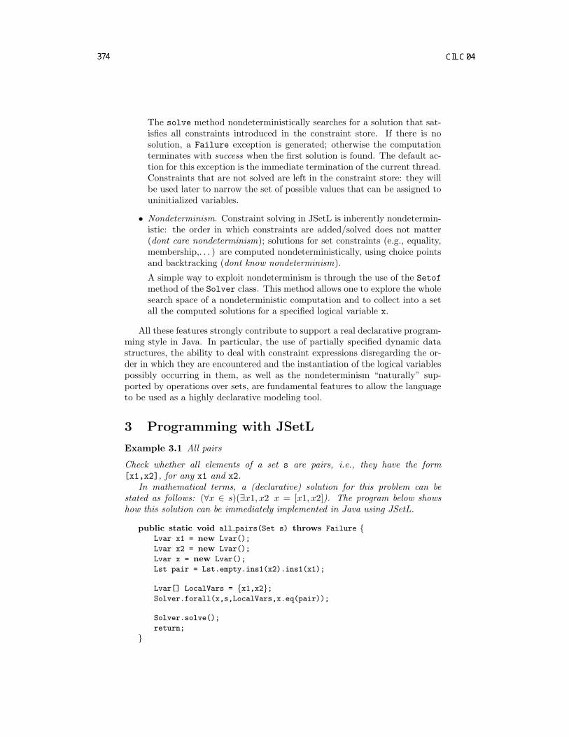
The solve method nondeterministically searches for a solution that sat-isfies all constraints introduced in the constraint store. If there is nosolution, a Failure exception is generated; otherwise the computationterminates with success when the first solution is found. The default ac-tion for this exception is the immediate termination of the current thread.Constraints that are not solved are left in the constraint store: they willbe used later to narrow the set of possible values that can be assigned touninitialized variables.

• Nondeterminism. Constraint solving in JSetL is inherently nondetermin-istic: the order in which constraints are added/solved does not matter(dont care nondeterminism); solutions for set constraints (e.g., equality,membership,. . . ) are computed nondeterministically, using choice pointsand backtracking (dont know nondeterminism).

A simple way to exploit nondeterminism is through the use of the Setofmethod of the Solver class. This method allows one to explore the wholesearch space of a nondeterministic computation and to collect into a setall the computed solutions for a specified logical variable x.

All these features strongly contribute to support a real declarative program-ming style in Java. In particular, the use of partially specified dynamic datastructures, the ability to deal with constraint expressions disregarding the or-der in which they are encountered and the instantiation of the logical variablespossibly occurring in them, as well as the nondeterminism “naturally” sup-ported by operations over sets, are fundamental features to allow the languageto be used as a highly declarative modeling tool.

3 Programming with JSetL

Example 3.1 All pairs

Check whether all elements of a set s are pairs, i.e., they have the form[x1,x2], for any x1 and x2.

In mathematical terms, a (declarative) solution for this problem can bestated as follows: (∀x ∈ s)(∃x1, x2 x = [x1, x2]). The program below showshow this solution can be immediately implemented in Java using JSetL.

public static void all pairs(Set s) throws Failure Lvar x1 = new Lvar();

Lvar x2 = new Lvar();

Lvar x = new Lvar();

Lst pair = Lst.empty.ins1(x2).ins1(x1);

Lvar[] LocalVars = x1,x2;Solver.forall(x,s,LocalVars,x.eq(pair));

Solver.solve();

return;

Example 3.1 shows the declaration of three logical variables, x1, x2, x, andthe creation of a new object of type Lst, representing a partially specified listof two elements. The constraints to be solved are introduced by the forallmethod, using the LocalVars array to specify existentially quantified (logical)variables. The call to the solve method allows to check satisfiability of thecurrent collection of constraints.

The next example is a method to compute the set of all subsets of a givenset. In this case we use the add method to introduce a new constraint and thesetof method to get all possible solutions (not only the first one).

Example 3.2 All solutions

Compute the powerset of a given set s.

public static Set powerset(Set s) throws Failure Set r = new Set();

Solver.add(r.subset(s));

return Solver.setof(r);

If s is the set ’a’,’b’, the set returned by powerset is ,’a’,’b’,’a’,’b’.

References

[1] A.Chun. Constraint programming in Java with JSolver. In Proc. PracticalApplications of Constraint Logic Programming, PACLP99, 1999.

[2] A. Dovier, C. Piazza, E. Pontelli, and G. Rossi. Sets and constraint logicprogramming. ACM TOPLAS, 22(5), 861–931, 2000.

[3] A. Dovier, E. Pontelli, and G. Rossi. Set unification. TR-CS-001/2001,Dept. of Computer Science, New Mexico State University, USA, January2001 (available at www.cs.nmsu.edu/TechReports).

[4] Neng-Fa Zhou. Building Java Applets by using DJ—a Java Based Con-straint Language. Available at www.sci.brooklyn.cuny.edu/~zhou.

Index of Authors

Alberti M. . . . . . . . . . . . . . . . . . . . . . . . . 13, 362

Alferes J. . . . . . . . . . . . . . . . . . . . . . . . . . . . . . 235

Backofen R. . . . . . . . . . . . . . . . . . . . . . . . . . . 103

Banti F. . . . . . . . . . . . . . . . . . . . . . . . . . . . . . . 235

Baldoni M. . . . . . . . . . . . . . . . . . . . . . . . . . . . 250

Baroglio C. . . . . . . . . . . . . . . . . . . . . . . . . . . . 250

Berardi M. . . . . . . . . . . . . . . . . . . . . . . . . . . . 220

Blandi L. . . . . . . . . . . . . . . . . . . . . . . . . . . . . . . 43

Boella G. . . . . . . . . . . . . . . . . . . . . . . . . . . . . . 265

Bonchi F. . . . . . . . . . . . . . . . . . . . . . . . . . . . . 202

Bortolussi L. . . . . . . . . . . . . . . . . . . . . . . . . . 362

Bossi A. . . . . . . . . . . . . . . . . . . . . . . . . . . . . . . 310

Brogi A. . . . . . . . . . . . . . . . . . . . . . . . . . . . . . .235

Buccafurri F.. . . . . . . . . . . . . . . . . . . . . . . . . .330

Cadoli M. . . . . . . . . . . . . . . . . . . . . . . . . . . . . 118

Caminiti G. . . . . . . . . . . . . . . . . . . . . . . . . . . 330

Capotorti A. . . . . . . . . . . . . . . . . . . . . . . . . . . 56

Chesani F. . . . . . . . . . . . . . . . . . . . . . . . . . . . 362

Citrigno M. . . . . . . . . . . . . . . . . . . . . . . . . . . 148

Cordı V. . . . . . . . . . . . . . . . . . . . . . . . . . . . . . 163

Costantini S. . . . . . . . . . . . . . . . . . . 7, 295, 368

Cumbo C. . . . . . . . . . . . . . . . . . . . . . . . . . . . . 178

D’Antonio M. . . . . . . . . . . . . . . . . . . . . . . . . . 73

Dal Palu A. . . . . . . . . . . . . . . . . . . . . . 103, 362

Delzanno G.. . . . . . . . . . . . . . . . . . . . . . . . . . . .73

Dovier A. . . . . . . . . . . . . . . . . . . . . . 8, 103, 362

Endriss U. . . . . . . . . . . . . . . . . . . . . . . . . . . . . . 28

Faber W. . . . . . . . . . . . . . . . . . . . . . . . . . . . . . 148

Formisano A. . . . . . . . . . . . . . . . . . . . . . . 56, 88

Gabbrielli M. . . . . . . . . . . . . . . . . . . . . . . . . . 345

Gavanelli M. . . . . . . . . . . . . . . . . . . . . . . 13, 362

Giannotti F. . . . . . . . . . . . . . . . . . . . . . . . . . .202

Greco G. . . . . . . . . . . . . . . . . . . . . . . . . . . . . . 148

Gungui I. . . . . . . . . . . . . . . . . . . . . . . . . . . . . .280

Iiritano S. . . . . . . . . . . . . . . . . . . . . . . . . . . . . 178

Lamma E. . . . . . . . . . . . . . . . . . . . . . . . . 13, 362

Leone N. . . . . . . . . . . . . . . . . . . . . . . . . . . . . . 148

Majkic Z. . . . . . . . . . . . . . . . . . . . . . . . . . . . . 189

Malerba D. . . . . . . . . . . . . . . . . . . . . . . . . . . . 220

Mancarella P. . . . . . . . . . . . . . . . . . . . . . . . . . .28

Mancini T. . . . . . . . . . . . . . . . . . . . . . . . . . . . 118

Martelli A. . . . . . . . . . . . . . . . . . . . . . . . . . . . 250

Mascardi V. . . . . . . . . . . . . . . . . . . . . . 163, 280

Mello P. . . . . . . . . . . . . . . . . . . . . . . . . . . 13, 362

Meo M. C. . . . . . . . . . . . . . . . . . . . . . . . . . . . 345

Omodeo E. G. . . . . . . . . . . . . . . . . . . . . . . . . . 88

Orlowska E. S. . . . . . . . . . . . . . . . . . . . . . . . . .88

Panegai E. . . . . . . . . . . . . . . . . . . . . . . . . . . . 372

Patti V. . . . . . . . . . . . . . . . . . . . . . . . . . . . . . . 250

Pedreschi D. . . . . . . . . . . . . . . . . . . . . . . . . . .202

Pereira L. M. . . . . . . . . . . . . . . . . . . . . . . . . . . . 3

Pettorossi A. . . . . . . . . . . . . . . . . . . . . . . . . . 325

Piazza C. . . . . . . . . . . . . . . . . . . . . . . . . . . . . .310

Pinto A. M. . . . . . . . . . . . . . . . . . . . . . . . . . . . . 3

Poleo E. . . . . . . . . . . . . . . . . . . . . . . . . . . . . . . 372

Policriti A. . . . . . . . . . . . . . . . . . . . . . . . . . . . . 88

Prestwich S. . . . . . . . . . . . . . . . . . . . . . . . . . . 133

Proietti M. . . . . . . . . . . . . . . . . . . . . . . . . . . . 325

Rossi F. . . . . . . . . . . . . . . . . . . . . . . . . . . . . . . 133

Rossi G. . . . . . . . . . . . . . . . . . . . . . . . . . . . . . . 372

Rossi S. . . . . . . . . . . . . . . . . . . . . . . . . . . . . . . 310

Rullo P. . . . . . . . . . . . . . . . . . . . . . . . . . . . . . . 178

Sadri F. . . . . . . . . . . . . . . . . . . . . . . . . . . . . . . . 28

Sessa M.I. . . . . . . . . . . . . . . . . . . . . . . . . . . . . . 43

Terreni G. . . . . . . . . . . . . . . . . . . . . . . . . . . . . . 28

Tocchio A. . . . . . . . . . . . . . . . . . . . . . . .295, 368

Toni F. . . . . . . . . . . . . . . . . . . . . . . . . . . . . . . . . 28

Torasso L. . . . . . . . . . . . . . . . . . . . . . . . . . . . . 217

1

Torre var der L. . . . . . . . . . . . . . . . . . . . . . . 265

Torroni P. . . . . . . . . . . . . . . . . . . . . . . 9, 13, 362

Varlaro A. . . . . . . . . . . . . . . . . . . . . . . . . . . . . 220

Venable B. K. . . . . . . . . . . . . . . . . . . . . . . . . 133

Verticchio A. . . . . . . . . . . . . . . . . . . . . . . . . . 295

Walsh T. . . . . . . . . . . . . . . . . . . . . . . . . . . . . . 133

Will S. . . . . . . . . . . . . . . . . . . . . . . . . . . . . . . . 103

Stampato in proprio dal Dipartimento di Matematica dell’Universita degliStudi di Parma in Via M. D’Azeglio 85/A, 43100 Parma, adempiuti gli obb-lighi di cui all’articolo 1 del D.L. 31 agosto 1945 n. 660.