Quadrilateral et HexahedralPseudo-conform Finite Elements

E. DUBACH, R. LUCE, J.M. THOMASLaboratoire de Mathématiques Appliquées, UMR 5142, Pau (France)GDR MoMas

Méthodes Numériques pour les Fluides. Paris 20 décembre 2006

What is the problem?

Loss of convergence for the RT, BDM, BDFM

when we use quadrilateral or hexahedral elements.

( )

hhhhhh

hhhhh

hhhh

KhhhKhhh

LdxpdxA

Mqdxqdxq

MLp

KPqLqMKRTdivHL

∈∀=∇−

∈∀=+

×∈

∈Ω∈=∈Ω∈=

∫∫

∫∫

ΩΩ

−

ΩΩ

vvvu

u

u

vv

0

0fdiv

of solution, find

)();(,)();,(

:modelStandart

1

0

2

0

uh does not converge in H(div) when the mesh is based on

quadrilateral or hexahedral elements.

−5.5−5−4.5−4−3.5−3−2.5−2−1.5−1−6

−5

−4

−3

−2

−1

0

1

2

log(pas)

log

(err

eu

r)

||u−uh||0,Ω

==> 0.99621 ||p−ph||0,Ω

==> 0.98933 ||div(u−uh)||

0,Ω==> 0.14476

2D

Loss of convergence on div(u)

3D

Loss of convergence on u and div(u)

Where does the problem come from?

element reference

tion triangula theofelement

:ˆ

:

K

K

F is bilinear

21det(DF) PQJ F ∩∈=

F is trilinear

42det(DF) PQJ F ∩∈=

)x(ˆ(x)),x(u)xDF()x(

u(x) ppJ F

== 1

∫∫∫∫ ==∂∂ KKKK

dxpdivpdxdivsdppdsˆˆ

ˆuu,ˆˆn.un.u

Piola transform:

u(x))xM()x(u =

u(x))x()x(u divJdiv F=Non linear relations

ΩΩ≤−

,,uπu

10uChh

ΩΩ≤−

,,uu)π(u10

divCdiv h

ΩΩ≤−

,,uuu10

Chπ

ΩΩ≤−

,1,0)( uuπu divCdiv h

2D 3D

Solutions

- Increase the space of discretisation to control the non-linear part of

the transformation F. (Arnold-Boffi-Falk, 2004 (2D))

2D Parallelogram (RT0) Quadrilateral (ABF0)

Degrees of freedom: 4 Degrees of freedom: 4+2=6

3D Parallelepiped (RT0) Hexahedron

Degrees of freedom: 6 Degrees of freedom: 36!!

By using the same way, we obtain

- « Remesh » the quadrilaterals or hexahedrals

Yu. Kuznetsov and S. Repin (J. Numer. Math 2005)

- Build pseudo-conform finite elements without adding

degrees of freedom

Solutions

We have chosen this last way

Obviously it is a possibility

Let us examine the Q1 conform approximation on quadrilaterals. Why?

Cas 2D

No loss of convergence with the Q1 finite element but the background is

different of the P1 finite element on triangles

Work on is equivalent

to work on T

T

11ˆ PPˆ ∈⇔∈TT

pp

polynomialnot is

QQˆ11ˆ

K

KK

p

pp ∉⇒∈

Consequence: All the integrals must be calculated on K^

xdJvDFpDFdxvp

pDFp

FhK

hhK

h

hh

ˆˆ.ˆ.

ˆ

1

ˆ

1

1

∇∇=∇∇

∇=∇−−

−

∫∫

Goal:

Construct a new finite element satisfying:

• ph is polynomial on K

• Degrees of freedom are the same

• On parallelogram, recover the classical “Q1 finite element”

Price to pay:

• The degree of the polynomials must be increased.

• The approximation is pseudo-conform

Geometry and notations

ralquadrilateconvex a :R2⊂K

[ ] 4,...,1 ,, :edges ,:vertices 1 == + iiiii aaa γ

)(4

1: ofcenter 43210 aaaaa +++=K

)(4

1

)(4

1

by given of basis the),(

43212

43211

2

21

aaaa

aaaa

++−−=

−++−=

e

e

Ree K

KK

KK

ˆ squareunit theof ndeformatioa is

into ed transformis , By. ofpart affine :

#

### FFF

KK#

F#

1ralquadrilateconvex K 21 <+=⇔ ddK

d

),,(Kelement finitenew a of onConstructi ## ,1

#

KKP Σ

41),( #

,1 # ≤≤→=Σ iww iKaWe want

? of Choice #KP

1# QPK

=a

We obtain a non conforming approximation that does not satisfy the patch-test.

In the error estimation, we don’t control the following term:

[ ] σγ

dIn

hh

ii

uuu −

∂∂

∑∫

[ ] 0 that such find :Solutioni

# =∫ σγ

dP hKu

Proposition:

For any convex quadrilateral K there exist a

polynomial ωK# such that for the choice:

),( ## 1 KKPVectP ω=

We have

)4...,1()()(2

)2

element. finitea is ),,(K)1

#

1

#

,1

#

#

#

##

=+=∈∀°

Σ°

+∫ iwwwdPw

P

ii

i

K

KK

i

aa

γ

γσ

uniquenot is :Remark #Kω

#1 havemust WeKPP ⊂

Moreover, it is of interest to obtain:

squareunit theonelement finite reference Lagrange the

)ˆ,,K(),,(Kelement finite the0, limite at the

parameter distorsion theony continousl depend

1,1

###

#

Σ=Σ=•

•

QPKK

K

d

dω

( )

∫ ==

=−=

∩+

#

#

#

#

4,...,10

4,...,11)(

:satisfying in choose tois choicesimplest The

K

1

K

23K

i

id

i

QP

i

i

γ

σω

ω

ω

a

ynumericallor toaccordingy explicitel calculated be can # dK

ω

Remark: We can computed the finite element basis in without

calculating ωK#

23 QP ∩

0 0.2 0.4 0.6 0.8 10

0.1

0.2

0.3

0.4

0.5

0.6

0.7

0.8

0.9

1

0 0.2 0.4 0.6 0.8 10

0.1

0.2

0.3

0.4

0.5

0.6

0.7

0.8

0.9

1

Mesh in “chevron” Mesh in “alvéole”

))(1)()(1)(1)(1( with

))221(

)221(

)2322322272221(

)1)(1)(1(3(1

),(

2

21

2

21

2

2

2

1

2#

2

#

11

4

2

2

2

2

1

4

1

2

2

2

1

#

2

2#

12

4

2

2

2

2

1

4

1

2

2

2

1

#

2

#

1

2

2

4

1

4

2

2

1

4

2

2

2

2

1

4

1

2

2

2

1

2#

2

2#

1

2

2

2

121

#

2

#

1#

ddddddden

xxddddddd

xxddddddd

xxdddddddddd

xxddddden

xxK

−−+−−−=

+−−−+−+

+−++−−+

−−+++−−+

−−−−−=ω

Q1 conform Pseudo-conform method

),,(Kelement finitenew a of onConstructi *

,1

*### KK

P Σ

≤≤→=Σ ∫#

# 41,. want We *

,1

i

idK

γ

σnww

),,( ##

#

00

*

KKPPvectP ψx×=

Let us return to the initial problem

Proposition:

For any convex quadrilateral K there exist a polynomial

vector ψψψψK# such that for the choice:

We have

)4...,1(.1

.

,)2

element. finitea is ),,(K)1

#

#

##

1

*

*

,1

*#

=

=

∈∀∈∀°

Σ°

∫∫ ∫ idsdds

PsP

P

ii ii

K

KK

γγ γ

σσγ

σ nwnw

w

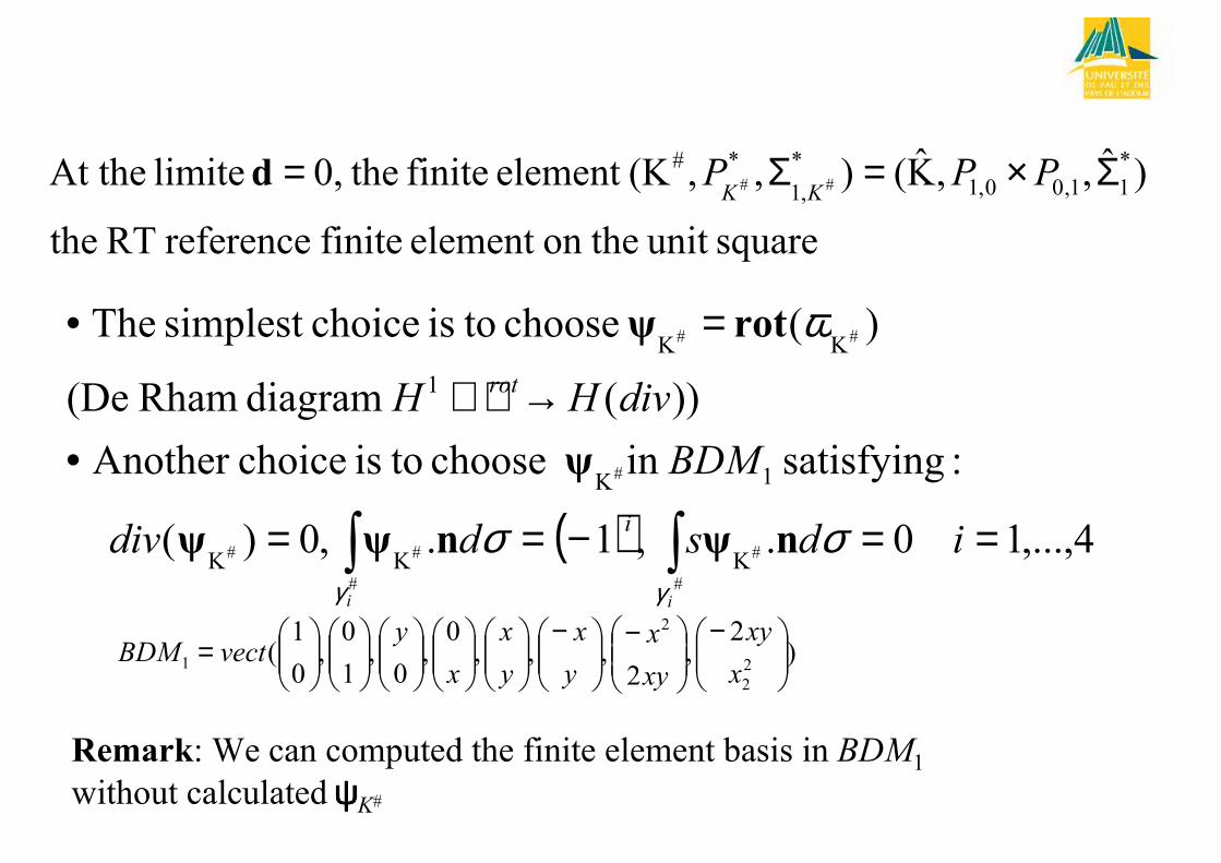
squareunit theonelement finite reference RTthe

)ˆ,,K(),,(Kelement finite the0, limite At the *

11,00,1

*

,1

*### Σ×=Σ= PPP

KKd

( ) ∫∫ ==−==

•→

=•

#

#

#

##

#

##

4,...,10.,1.,0)(

:satisfying in choose tois choiceAnother

))( diagram Rham(De

)( choose tois choicesimplest The

KKK

1K

1

KK

ii

idsddiv

BDM

divHH

i

rot

γγ

σσ

ω

nψnψψ

ψ

rotψ

Remark: We can computed the finite element basis in BDM1without calculated ψψψψK#

)2

,2

,,,0,

0,

1

0,

0

1(

2

2

2

1

−

−

−

=x

xy

xy

x

y

x

y

x

x

yvectBDM

−5.5−5−4.5−4−3.5−3−2.5−2−1.5−1−6

−5

−4

−3

−2

−1

0

1

2

log(pas)

log(

erre

ur)

||u−uh||0,Ω

==> 0.99661 ||p−ph||0,Ω

==> 0.99364 ||div(u−uh)||

0,Ω==> 0.99431

The convergence orders are good

Conclusion

• If the quadrilaterals K are parallelograms we have

)ˆ,,ˆ(),,( 1,1

### Σ=Σ QKPK

KK

and the approximations are conform.

• If the quadrilaterals K are not parallelograms the approximations are not

conform.

The use of allows us to have the continuity of ph at the

nodes and only the continuity of the mean values through each edge of

the mesh.

The use of allows us to have the continuity of the

mean value of uh.n and the continuity of the first momentum of uh.n

through each edge.

• The implementation is simple, but the basis functions depend on of the

shape of K.

)ˆ,,ˆ(),,( *

11,00,1

*

,1

*### Σ×=Σ PPKPK

KK

),,( ## ,1

#

KKPK Σ

)ˆ,,ˆ( *

11,00,1 Σ× PPK

3D case

We apply the same approach with the 3D case.

• Plane faces and non-plane faces? Is it a real problem?

Problems with the hexahedrons

• Parametrisation of the faces

• Description of a hexahedron (deformation of the unit cube)

3D case

K#

K# depends on 6 parameters if the

faces are plane and 9 parameters if

the faces are not plane.

K)

∫ ∫=# ˆ

### ˆˆ)ˆ())ˆ(()(

i i

dvdv i

γ γ

σσ nxMxxx

polynomialnot is ˆ)ˆ( : face plane non

ˆ)ˆ( :face plane 1

i

i P

nxM

nxM ∈

faces) plane of (case ?built How to #KP

),,(element finitenew a of onConstructi ## ,1

#

KKPK Σ

81),( want We #

,1 # ≤≤→=Σ iww iKa

KKV

ivdwiwwΣ

VP

Vdim

V

K

i,K

K

K

K

i

ˆ when on unisolvant is

)6...1,;8...1),(

14)(

thatsuch space polynomiala beLet

#

#

2

1

#

##

#

#

#

=

=→=→=•

⊂•

=•

∫γ σa

1,...,4)j,( pointsat jacobian the

ofmatrix cofacteur theof values theononly depend

, face theof node theof numbers serial are )4,...,1),(( where

6,...,1)()(

#

)(

,

#

4

1

#

)(,

##

1

#

#

#

=

=

==∈∀ ∫ ∑=

jl

j

ii

j

jlj

i

i

i

ii

jjl

ivvdKPv

a

a

γ

γγ

ωγ

ωσ

Building of integration formulas

==∈= ∫ ∑=

6,...,1)(;#

###

4

1

#

)(,

#** ivvdsVvP

i

iij

jljjKK

γγωσ a

Possible choices of polynomial space #KV

23

222222 ,,,,,,,,,,,,,1# QPxzzyyxzyxxyzyzxzxyzyxVK

∩⊂=•

)1)(1)(1()1)(1)(1(

)1)(1)(1()1)(1)(1(

)1)(1)(1()1)(1)(1()(

2222

2222

2222#

1#

yxzyxz

xzyxzy

zyxzyxKQVK

+−−⊕−−−⊕+−−⊕−−−⊕

+−−⊕−−−⊕=•

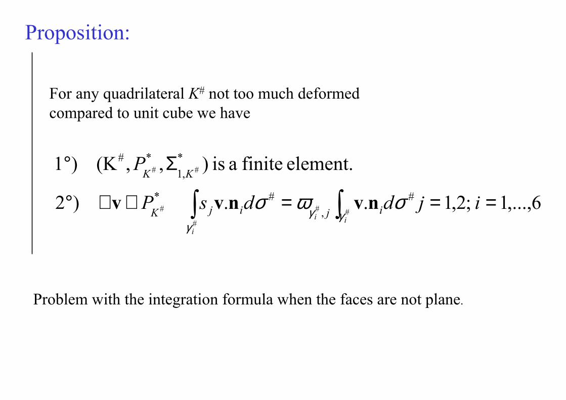
Proposition:

For any quadrilateral K# not too much deformed

compared to unit cube we have

6,...,1)()2

element. finitea is ),,(K)1

#

##

##

4

1

#

)(,

#

,1

#

==∈∀°

Σ°

∫ ∑=

ivvdPv

P

i

iij

jljK

KK

γγωσ a

Remark: The main difference, when the faces are not plane, concerns the integration formulas:

case plane-non thein calculatedy numericall bemust

case plane thein known explicitly are

,

,

#

#

j

j

i

i

γ

γ

ω

ω

00.2

0.40.6

0.81

0

0.5

10

0.2

0.4

0.6

0.8

1

Non plane faces

Interior faces are not plane

Destructured mesh

Q1 conform

Pseudo-conform method==>

Non-plane faces

Plane faces

What’s about the approximation in Hdiv

),,(Kelement finitenew a of onConstructi *

,1

*### KK

P Σ

≤≤→=Σ ∫#

# 61,. want We *

,1

i

idiK

γ

σnww

?built How to *#K

P

KKV

jidswidΣ

VP

Vdim

V

K

j,K

K

K

K

ii

ˆ when on unisolvant is

)2,1,6...1,.;6...1,.

18)(

thatsuch space polynomiala beLet

#

##*

2

*

0,0,0

*

*

#

###

#

#

#

=

==→=→=•

⊂•

=•

∫∫ γγσσ nunuu

. on jacobian the

ofmatrix cofacteur theof valuesononly depend

6,...,1;2,1..)(

#

,

#

,

##

0,0,0

#

#

##

i

j

ijij

i

i

ii

ijddsKP

γ

ω

σωσ

γ

γγγ ===∈∀ ∫ ∫ nvnvv

Building of integration formulas

===∈= ∫ ∫ 6,...,1;2,1..;#

####

#

,

#** ijddsVP

i

iiijijKK

γγγ σωσ nvnvv

Possible choice of polynomial space 1

*# BDMV

K=

)0,

0

,

0

,

0

2

,0

2

,

0

2,,

0

,0,0

0

,0

0

,

0

0

,

0

0

,

0

0,

0

0,

1

0

0

,

0

1

0

,

0

0

1

( 2

2

2

1

−

−

−

−

−

−

−

−

=yz

xy

yz

xz

xz

xyy

xy

z

xz

xy

x

z

y

x

y

x

z

x

yx

zx

zy

vectBDM

Proposition:

For any quadrilateral K# not too much deformed

compared to unit cube we have

6,...,1;2,1..)2

element. finitea is ),,(K)1

#

###

##

#

,

#*

*

,1

*#

===∈∀°

Σ°

∫ ∫ ijddsP

P

i

iiijijK

KK

γγγ σωσ nvnvv

Problem with the integration formula when the faces are not plane.

Pseudo-conform method (plane faces)

Conclusions

• 2D case:

• The numerical results are agree with the theoretical results.• Possibility to generalise the results to FEM of higher degrees.

• 3D case:

• Necessity to work on the geometry of the hexahedrons.

• Clarify the problem of plane faces and non-plane faces.

• Use the De Rham diagram to connect the H1 case to the H(div) case

))()( :diagram Rham(De 1 divHcurlHHrot→→∇