quadrotor control: modeling, nonlinear control design, and .../thesis kth... · quadrotor control:...
TRANSCRIPT
Quadrotor control: modeling, nonlinearcontrol design, and simulation
FRANCESCO SABATINO
Master’s Degree ProjectStockholm, Sweden June 2015
XR-EE-RT 2015:XXX

Abstract
In this work, a mathematical model of a quadrotor’s dynamics is derived, usingNewton’s and Euler’s laws. A linearized version of the model is obtained, andtherefore a linear controller, the Linear Quadratic Regulator, is derived. Afterthat, two feedback linearization control schemes are designed. The first one isthe dynamic inversion with zero dynamics stabilization, based on Static Feed-back Linearization obtaining a partial linearization of the mathematical model.The second one is the exact linearization and non-interacting control via dynamicfeedback, based on Dynamic Feedback Linearization obtaining a total lineariza-tion of the mathematical model. Moreover, these nonlinear control strategiesare compared with the Linear Quadratic Regulator in terms of performances.Finally, the behavior of the quadrotor under the proposed control strategies isobserved in virtual reality by using the Simulink 3D Animation toolbox.
i

ii
Contents
1 Introduction 11.1 Literature review . . . . . . . . . . . . . . . . . . . . . . . . . . . 2
1.1.1 Quadrotor history . . . . . . . . . . . . . . . . . . . . . . . 21.1.2 Control . . . . . . . . . . . . . . . . . . . . . . . . . . . . 4
1.2 Outline . . . . . . . . . . . . . . . . . . . . . . . . . . . . . . . . . 5
2 Mathematical model 72.1 Preliminar notions . . . . . . . . . . . . . . . . . . . . . . . . . . 72.2 Euler angles . . . . . . . . . . . . . . . . . . . . . . . . . . . . . . 102.3 Quadrotor mathematical model . . . . . . . . . . . . . . . . . . . 122.4 Forces and moments . . . . . . . . . . . . . . . . . . . . . . . . . 142.5 Actuator dynamics . . . . . . . . . . . . . . . . . . . . . . . . . . 152.6 State-space model . . . . . . . . . . . . . . . . . . . . . . . . . . . 152.7 Linear model . . . . . . . . . . . . . . . . . . . . . . . . . . . . . 18
2.7.1 Linearization . . . . . . . . . . . . . . . . . . . . . . . . . 192.7.2 Controllability and observability of the linear system . . . 21
3 Control strategies 253.1 Linear Quadratic Regulator control . . . . . . . . . . . . . . . . . 253.2 Feedback linearization control . . . . . . . . . . . . . . . . . . . . 28
3.2.1 Exact linearization and non-interacting control via dynamicfeedback . . . . . . . . . . . . . . . . . . . . . . . . . . . . 30
3.2.2 Dynamic inversion with zero-dynamics stabilization . . . . 37
4 Simulation results 414.1 Linear Quadratic Regulator results . . . . . . . . . . . . . . . . . 414.2 Exact linearization and non-interacting control via dynamic feed-
back results . . . . . . . . . . . . . . . . . . . . . . . . . . . . . . 434.3 Dynamic inversion with zero-dynamics stabilization results . . . . 454.4 Comparison . . . . . . . . . . . . . . . . . . . . . . . . . . . . . . 474.5 3D Animation . . . . . . . . . . . . . . . . . . . . . . . . . . . . . 49
5 Conclusions and future developments 51
A Input-output Feedback Linearization 53
iii

iv Contents
Chapter 1
Introduction
Recent advances in sensor, in microcomputer technology, in control and in aero-dynamics theory have made small Unmanned Aerial Vehicles (sUAV) a reality.The small size, low cost and maneuverability of these systems have made thempotential solutions in a large class of applications. However, the small size ofthese vehicles poses significant challenges. The small sensors used on these sys-tems are much noisier than their larger counterparts. The compact structure ofthese vehicles also makes them more vulnerable to environmental effects. In thiswork, control strategies for an sUAV platform are developed. Simulation studiesand experimental results are provided.The fundamental problem with the safe operation of vehicles with wingspansmaller than one meter is reliable stabilization, robustness to unpredictablechanges in the environment, and resilience to noisy data from small sensor sys-tems. Autonomous operation of aerial vehicles relies upon on-board stabilizationand trajectory tracking capabilities, and significant effort has to be carried onto make sure that these systems are able to achieve stable flight. These prob-lems are compounded at smaller scale, since as the vehicle is more susceptible toenvironmental effects (wind, temperature, etc.). Moreover, the small scale im-plies that lower quality and noisier compact Micro-Electro-Mechanical Systems(MEMS) sensor are used as primary sensor. The small scale also makes it harderfor the MEMS sensors to be isolated from the vibrations that are common inthese flight platforms.Since the number and complexity of applications for such systems grows daily,the control techniques involved must also improve in order to provide betterperformance and increased versatility. Historically, simplistic linear control tech-niques were employed for computational ease and stable hover flight. However,with better modelling techniques and faster on board computational capabili-ties, comprehensive nonlinear techniques to be run on real-time have become anachievable goal. Nonlinear methodologies promise to rapidly increase the per-formances for these systems and make them more robust. This work presentsseveral approaches to the automatic control of a quadrotor. Selected linear andnonlinear control methods are designed according to the system dynamics.
1
2 Chapter 1 Introduction
1.1 Literature review
1.1.1 Quadrotor history
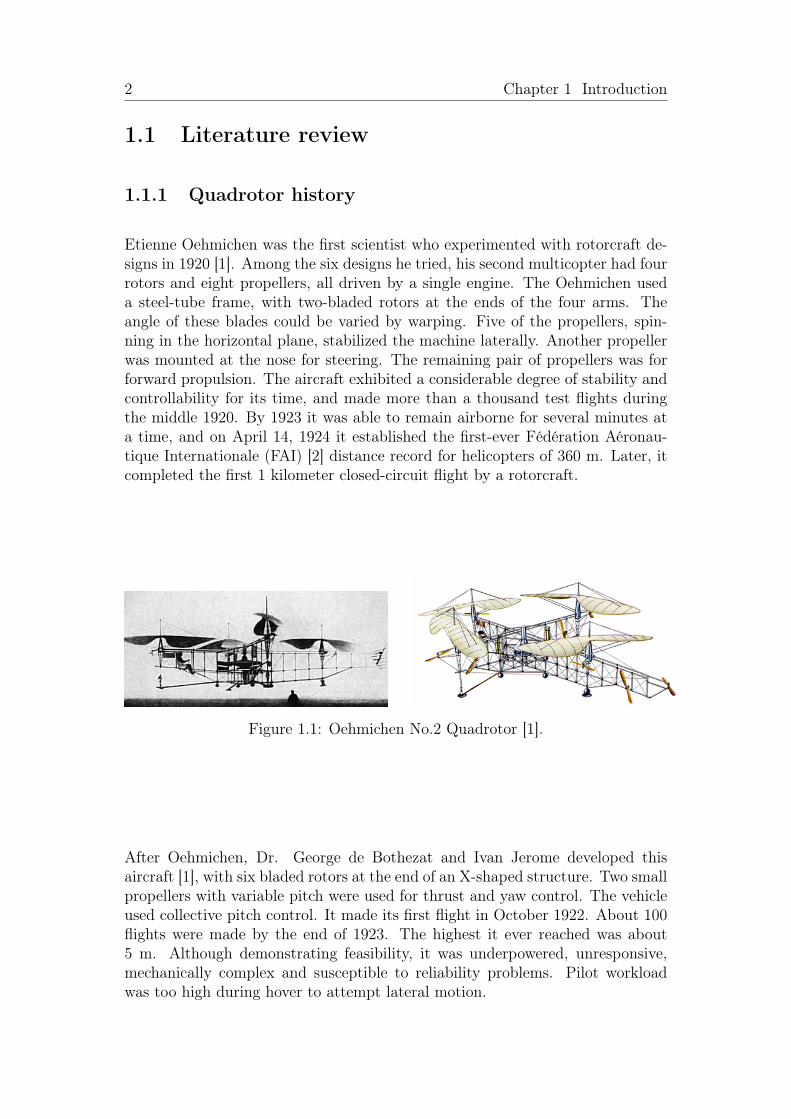
Etienne Oehmichen was the first scientist who experimented with rotorcraft de-signs in 1920 [1]. Among the six designs he tried, his second multicopter had fourrotors and eight propellers, all driven by a single engine. The Oehmichen useda steel-tube frame, with two-bladed rotors at the ends of the four arms. Theangle of these blades could be varied by warping. Five of the propellers, spin-ning in the horizontal plane, stabilized the machine laterally. Another propellerwas mounted at the nose for steering. The remaining pair of propellers was forforward propulsion. The aircraft exhibited a considerable degree of stability andcontrollability for its time, and made more than a thousand test flights duringthe middle 1920. By 1923 it was able to remain airborne for several minutes ata time, and on April 14, 1924 it established the first-ever Fédération Aéronau-tique Internationale (FAI) [2] distance record for helicopters of 360 m. Later, itcompleted the first 1 kilometer closed-circuit flight by a rotorcraft.
Figure 1.1: Oehmichen No.2 Quadrotor [1].
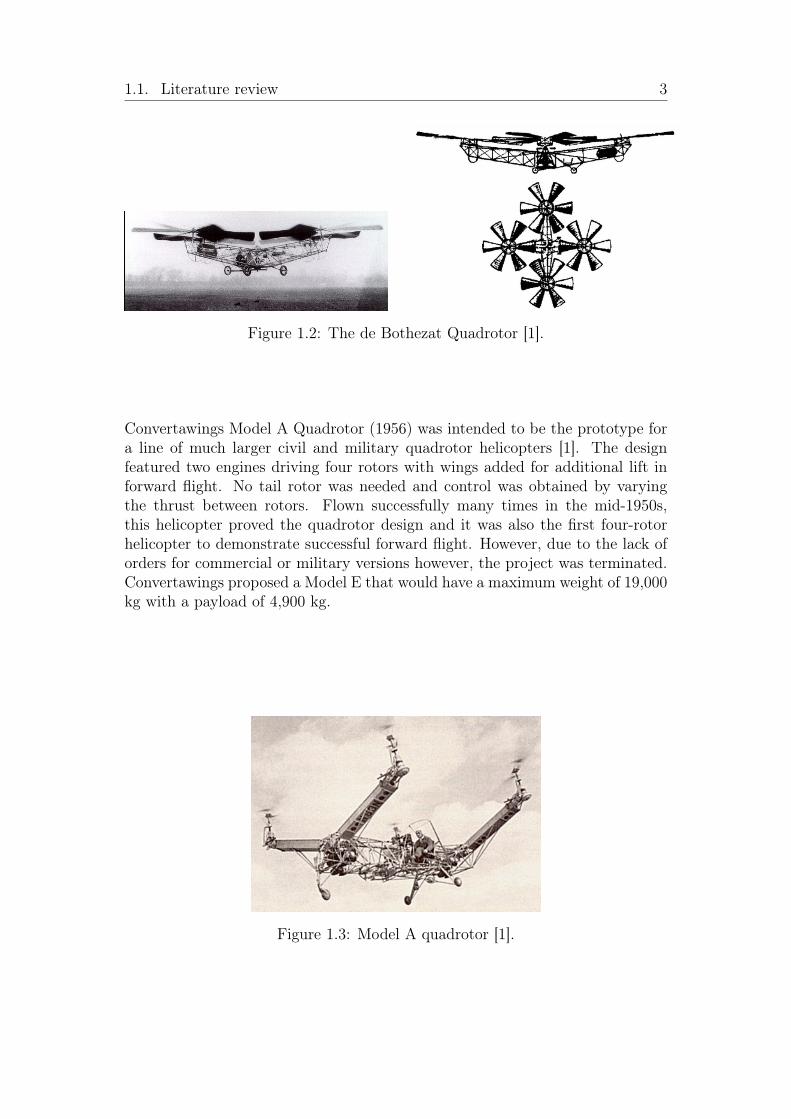
After Oehmichen, Dr. George de Bothezat and Ivan Jerome developed thisaircraft [1], with six bladed rotors at the end of an X-shaped structure. Two smallpropellers with variable pitch were used for thrust and yaw control. The vehicleused collective pitch control. It made its first flight in October 1922. About 100flights were made by the end of 1923. The highest it ever reached was about5 m. Although demonstrating feasibility, it was underpowered, unresponsive,mechanically complex and susceptible to reliability problems. Pilot workloadwas too high during hover to attempt lateral motion.
1.1. Literature review 3
Figure 1.2: The de Bothezat Quadrotor [1].
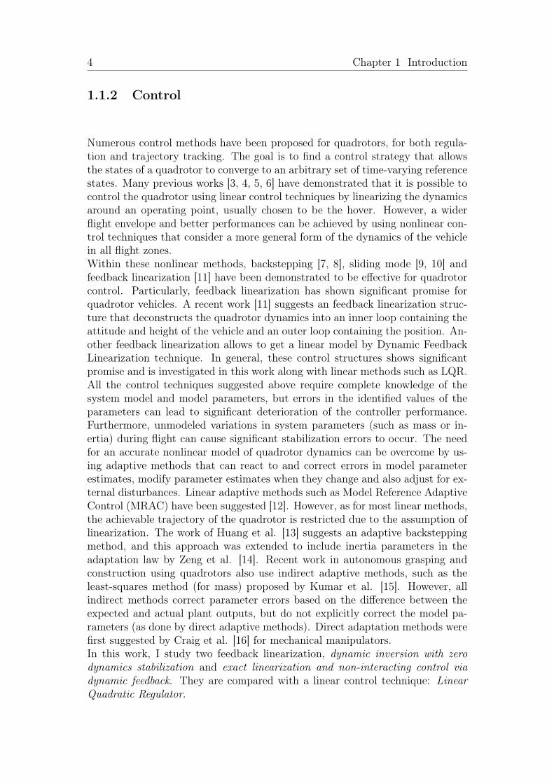
Convertawings Model A Quadrotor (1956) was intended to be the prototype fora line of much larger civil and military quadrotor helicopters [1]. The designfeatured two engines driving four rotors with wings added for additional lift inforward flight. No tail rotor was needed and control was obtained by varyingthe thrust between rotors. Flown successfully many times in the mid-1950s,this helicopter proved the quadrotor design and it was also the first four-rotorhelicopter to demonstrate successful forward flight. However, due to the lack oforders for commercial or military versions however, the project was terminated.Convertawings proposed a Model E that would have a maximum weight of 19,000kg with a payload of 4,900 kg.
Figure 1.3: Model A quadrotor [1].
4 Chapter 1 Introduction
1.1.2 Control
Numerous control methods have been proposed for quadrotors, for both regula-tion and trajectory tracking. The goal is to find a control strategy that allowsthe states of a quadrotor to converge to an arbitrary set of time-varying referencestates. Many previous works [3, 4, 5, 6] have demonstrated that it is possible tocontrol the quadrotor using linear control techniques by linearizing the dynamicsaround an operating point, usually chosen to be the hover. However, a widerflight envelope and better performances can be achieved by using nonlinear con-trol techniques that consider a more general form of the dynamics of the vehiclein all flight zones.Within these nonlinear methods, backstepping [7, 8], sliding mode [9, 10] andfeedback linearization [11] have been demonstrated to be effective for quadrotorcontrol. Particularly, feedback linearization has shown significant promise forquadrotor vehicles. A recent work [11] suggests an feedback linearization struc-ture that deconstructs the quadrotor dynamics into an inner loop containing theattitude and height of the vehicle and an outer loop containing the position. An-other feedback linearization allows to get a linear model by Dynamic FeedbackLinearization technique. In general, these control structures shows significantpromise and is investigated in this work along with linear methods such as LQR.All the control techniques suggested above require complete knowledge of thesystem model and model parameters, but errors in the identified values of theparameters can lead to significant deterioration of the controller performance.Furthermore, unmodeled variations in system parameters (such as mass or in-ertia) during flight can cause significant stabilization errors to occur. The needfor an accurate nonlinear model of quadrotor dynamics can be overcome by us-ing adaptive methods that can react to and correct errors in model parameterestimates, modify parameter estimates when they change and also adjust for ex-ternal disturbances. Linear adaptive methods such as Model Reference AdaptiveControl (MRAC) have been suggested [12]. However, as for most linear methods,the achievable trajectory of the quadrotor is restricted due to the assumption oflinearization. The work of Huang et al. [13] suggests an adaptive backsteppingmethod, and this approach was extended to include inertia parameters in theadaptation law by Zeng et al. [14]. Recent work in autonomous grasping andconstruction using quadrotors also use indirect adaptive methods, such as theleast-squares method (for mass) proposed by Kumar et al. [15]. However, allindirect methods correct parameter errors based on the difference between theexpected and actual plant outputs, but do not explicitly correct the model pa-rameters (as done by direct adaptive methods). Direct adaptation methods werefirst suggested by Craig et al. [16] for mechanical manipulators.In this work, I study two feedback linearization, dynamic inversion with zerodynamics stabilization and exact linearization and non-interacting control viadynamic feedback. They are compared with a linear control technique: LinearQuadratic Regulator.
1.2. Outline 5
1.2 OutlineThe rest of this thesis is organized as follows.
Chapter 2. In this chapter a qualitative introduction on the principles of work-ing of a quadrotor is discussed. Then the mathematical model is presented anda linearized version of the model is obtained.
Chapter 3. In this chapter a linear controller, the Linear Quadratic Regu-lator, is derived and two feedback linearization control schemes are designed.The first one is the dynamic inversion with zero dynamics stabilization, based onStatic Feedback Linearization obtaining a partial linearization of the mathemat-ical model. The second one is the exact linearization and non-interacting controlvia dynamic feedback, based on Dynamic Feedback Linearization obtaining atotal linearization of the mathematical model.
Chapter 4. In this chapter results obtained with the different controllers areillustrated, and the differences are discussed. Finally, the behavior of the quadro-tor under the proposed control strategies is observed in virtual reality by usingthe Simulink 3D Animation toolbox.
Chapter 5. Finally, in this chapter, conclusions and possible future devel-opments of the work are presented.

6 Chapter 1 Introduction
Chapter 2
Mathematical model
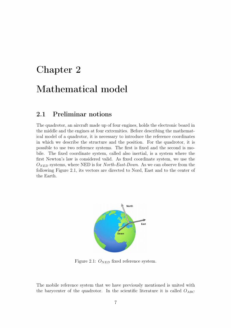
2.1 Preliminar notionsThe quadrotor, an aircraft made up of four engines, holds the electronic board inthe middle and the engines at four extremities. Before describing the mathemat-ical model of a quadrotor, it is necessary to introduce the reference coordinatesin which we describe the structure and the position. For the quadrotor, it ispossible to use two reference systems. The first is fixed and the second is mo-bile. The fixed coordinate system, called also inertial, is a system where thefirst Newton’s law is considered valid. As fixed coordinate system, we use theONED systems, where NED is for North-East-Down. As we can observe from thefollowing Figure 2.1, its vectors are directed to Nord, East and to the center ofthe Earth.
Figure 2.1: ONED fixed reference system.
The mobile reference system that we have previously mentioned is united withthe barycenter of the quadrotor. In the scientific literature it is called OABC
7
8 Chapter 2 Mathematical model
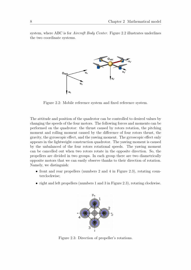
system, where ABC is for Aircraft Body Center. Figure 2.2 illustrates underlinesthe two coordinate systems.
Figure 2.2: Mobile reference system and fixed reference system.
The attitude and position of the quadrotor can be controlled to desired values bychanging the speeds of the four motors. The following forces and moments can beperformed on the quadrotor: the thrust caused by rotors rotation, the pitchingmoment and rolling moment caused by the difference of four rotors thrust, thegravity, the gyroscopic effect, and the yawing moment. The gyroscopic effect onlyappears in the lightweight construction quadrotor. The yawing moment is causedby the unbalanced of the four rotors rotational speeds. The yawing momentcan be cancelled out when two rotors rotate in the opposite direction. So, thepropellers are divided in two groups. In each group there are two diametricallyopposite motors that we can easily observe thanks to their direction of rotation.Namely, we distinguish:
• front and rear propellers (numbers 2 and 4 in Figure 2.3), rotating coun-terclockwise;
• right and left propellers (numbers 1 and 3 in Figure 2.3), rotating clockwise.
Figure 2.3: Direction of propeller’s rotations.
2.1. Preliminar notions 9
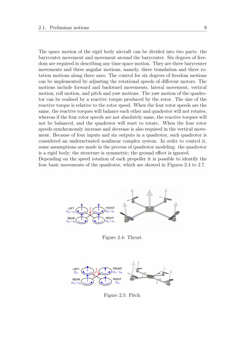
The space motion of the rigid body aircraft can be divided into two parts: thebarycenter movement and movement around the barycenter. Six degrees of free-dom are required in describing any time space motion. They are three barycentermovements and three angular motions, namely, three translation and three ro-tation motions along three axes. The control for six degrees of freedom motionscan be implemented by adjusting the rotational speeds of different motors. Themotions include forward and backward movements, lateral movement, verticalmotion, roll motion, and pitch and yaw motions. The yaw motion of the quadro-tor can be realised by a reactive torque produced by the rotor. The size of thereactive torque is relative to the rotor speed. When the four rotor speeds are thesame, the reactive torques will balance each other and quadrotor will not rotates,whereas if the four rotor speeds are not absolutely same, the reactive torques willnot be balanced, and the quadrotor will start to rotate. When the four rotorspeeds synchronously increase and decrease is also required in the vertical move-ment. Because of four inputs and six outputs in a quadrotor, such quadrotor isconsidered an underactuated nonlinear complex system. In order to control it,some assumptions are made in the process of quadrotor modeling: the quadrotoris a rigid body; the structure is symmetric; the ground effect is ignored.Depending on the speed rotation of each propeller it is possible to identify thefour basic movements of the quadrotor, which are showed in Figures 2.4 to 2.7.
Figure 2.4: Thrust.
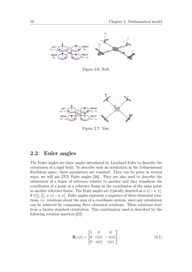
Figure 2.5: Pitch.
10 Chapter 2 Mathematical model
Figure 2.6: Roll.
Figure 2.7: Yaw.
2.2 Euler angles
The Euler angles are three angles introduced by Leonhard Euler to describe theorientation of a rigid body. To describe such an orientation in the 3-dimensionalEuclidean space, three parameters are required. They can be given in severalways; we will use ZYX Euler angles [26]. They are also used to describe theorientation of a frame of reference relative to another and they transform thecoordinates of a point in a reference frame in the coordinates of the same pointin another reference frame. The Euler angles are typically denoted as φ ∈]−π, π],θ ∈]π
2, π2[, ψ ∈]−π, π]. Euler angles represent a sequence of three elemental rota-
tions, i.e. rotations about the axes of a coordinate system, since any orientationcan be achieved by composing three elemental rotations. These rotations startfrom a known standard orientation. This combination used is described by thefollowing rotation matrices [27]:
Rx(φ) =
1 0 00 c(φ) −s(φ)0 s(φ) c(φ)
, (2.1)
2.2. Euler angles 11
Ry(θ) =
c(θ) 0 s(θ)
0 1 0−s(θ) 0 c(θ)
, (2.2)
Rz(ψ) =
c(ψ) −s(ψ) 0s(ψ) c(ψ) 0
0 0 1
, (2.3)
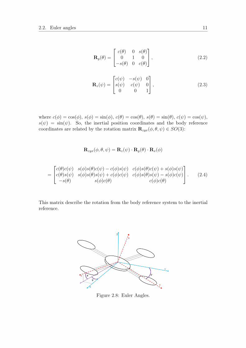
where c(φ) = cos(φ), s(φ) = sin(φ), c(θ) = cos(θ), s(θ) = sin(θ), c(ψ) = cos(ψ),s(ψ) = sin(ψ). So, the inertial position coordinates and the body referencecoordinates are related by the rotation matrix Rzyx(φ, θ, ψ) ∈ SO(3):
Rzyx(φ, θ, ψ) = Rz(ψ) ·Ry(θ) ·Rx(φ)
=
c(θ)c(ψ) s(φ)s(θ)c(ψ)− c(φ)s(ψ) c(φ)s(θ)c(ψ) + s(φ)s(ψ)c(θ)s(ψ) s(φ)s(θ)s(ψ) + c(φ)c(ψ) c(φ)s(θ)s(ψ)− s(φ)c(ψ)−s(θ) s(φ)c(θ) c(φ)c(θ)
. (2.4)
This matrix describe the rotation from the body reference system to the inertialreference.
Figure 2.8: Euler Angles.
12 Chapter 2 Mathematical model
2.3 Quadrotor mathematical model
We provide here a mathematical model of the quadrotor, exploiting Newton andEuler equations for the 3D motion of a rigid body. The goal of this section is toobtain a deeper understanding of the dynamics of the quadrotor and to providea model that is sufficiently reliable for simulating and controlling its behavior.Let us call
[x y z φ θ ψ
]T the vector containing the linear and angularposition of the quadrotor in the earth frame and
[u v w p q r
]T the vectorcontaining the linear and angular velocities in the body frame. From 3D bodydynamics, it follows that the two reference frames are linked by the followingrelations:
v = R · vB, (2.5)
ω = T · ωB, (2.6)
where v =[x y z
]T ∈ R3, ω =[φ θ ψ
]T ∈ R3, vB =[u v w
]T ∈ R3,ωB =
[p q r
]T ∈ R3, and T is a matrix for angular transformations [27]
T =
1 s(φ)t(θ) c(φ)t(θ)0 c(φ) −s(φ)
0 s(φ)c(θ)
c(φ)c(θ)
, (2.7)
where t(θ) = tan(θ). So, the kinematic model of the quadrotor is:
x = w[s(φ)s(ψ) + c(φ)c(ψ)s(θ)]− v[c(φ)s(ψ)− c(ψ)s(φ)s(θ)] + u[c(ψ)c(θ)]
y = v[c(φ)c(ψ) + s(φ)s(ψ)s(θ)]− w[c(ψ)s(φ)− c(φ)s(ψ)s(θ)] + u[c(θ)s(ψ)]
z = w[c(φ)c(θ)]− u[s(θ)] + v[c(θ)s(φ)]
φ = p+ r[c(φ)t(θ)] + q[s(φ)t(θ)]
θ = q[c(φ)]− r[s(φ)]
ψ = r c(φ)c(θ)
+ q s(φ)c(θ)
(2.8)
Newton’s law states the following matrix relation for the total force acting onthe quadrotor:
2.3. Quadrotor mathematical model 13
m(ωB ∧ vB + vB) = fB, (2.9)
wherem is the mass of the quadrotor, ∧ is the cross product and fB =[fx fy fz
]T ∈R3 is the total force.Euler’s equation gives the total torque applied to the quadrotor:
I · ωB + ωB ∧ (I · ωB) = mB, (2.10)
where mB =[mx my mz
]T ∈ R3 is the total torque and I is the diagonalinertia matrix:
I =
Ix 0 00 Iy 00 0 Iz
∈ R3×3.
So, the dynamic model of the quadrotor in the body frame is:
fx = m(u+ qw − rv)
fy = m(v − pw + ru)
fz = m(w + pv − qu)
mx = pIx − qrIy + qrIz
my = qIy + prIx − prIzmz = rIz − pqIx + pqIy
(2.11)
The equations stand as long as we assume that the origin and the axes of thebody frame coincide with the barycenter of the quadrotor and the principal axes.
14 Chapter 2 Mathematical model
2.4 Forces and momentsThe external forces in the body frame, fB are given by:
fB = mgRT · ez − fte3 + fw, (2.12)
where ez is the unit vector in the inertial z axis, e3 is the unit vector in thebody z axis, g is the gravitational acceleration, ft is the total thrust generatedby rotors and fw =
[fwx fwy fwz
]T ∈ R3 are the forces produced by wind onthe quadrotors. The external moments in the body frame, mB are given by
mB = τB − ga + τw, (2.13)
where ga represents the gyroscopic moments caused by the combined rotation ofthe four rotors and the vehicle body, τB =
[τx τy τz
]T ∈ R3 are the controltorques generated by differences in the rotor speeds and τw =
[τwx τwy τwz
]T ∈R3 are the torques produced by wind on the quadrotors. ga is given by
ga =4∑
i=1
Jp(ωB ∧ e3)(−1)i+1Ωi, (2.14)
where Jp is the inertia of each rotor and Ωi is the angular speed of the ith rotor.According to [18], the Jp term is found to be small and, for this reason, thegyroscopic moments are removed in the controller formulation. In addition, thereare numerous aerodynamic and aeroelastic phenomenon that affect the flight ofthe quadrotor, such as the ground effects: when flying close to the ground (orduring the landing stage), the air flow generated by the propellers disturbs thedynamics of the quadrotors. So, the complete dynamic model of the quadrotorin the body frame is obteined substituting the force expression in (2.11):
−mg[s(θ)] + fwx = m(u+ qw − rv)
mg[c(θ)s(φ)] + fwy = m(v − pw + ru)
mg[c(θ)c(φ)] + fwz − ft = m(w + pv − qu)
τx + τwx = pIx − qrIy + qrIz
τy + τwy = qIy + prIx − prIzτz + τwz = rIz − pqIx + pqIy
(2.15)
2.5. Actuator dynamics 15
2.5 Actuator dynamicsHere we consider the inputs that can be applied to the system in order to controlthe behavior of the quadrotor. The rotors are four and the degrees of freedom wecontrol are as many: commonly, the control inputs that are considered are onefor the vertical thrust and one for each of the angular motions. Let us considerthe values of the input forces and torques proportional to the squared speeds ofthe rotors [19]; their values are the following:
ft = b(Ω21 + Ω2
2 + Ω23 + Ω2
4)
τx = bl(Ω23 − Ω2
1)
τy = bl(Ω24 − Ω2
2)
τz = d(Ω22 + Ω2
4 − Ω21 − Ω2
3)
(2.16)
where l is the distance between any rotor and the center of the drone, b is thethrust factor and d is the drag factor. Substituting (2.16) in (2.15), we have: So,the dynamic model of the quadrotor in the body frame is:
−mg[s(θ)] + fwx = m(u+ qw − rv)
mg[c(θ)s(φ)] + fwy = m(v − pw + ru)
mg[c(θ)c(φ)] + fwz − b(Ω21 + Ω2
2 + Ω23 + Ω2
4) = m(w + pv − qu)
bl(Ω23 − Ω2
1) + τwx = pIx − qrIy + qrIz
bl(Ω24 − Ω2
2) + τwy = qIy + prIx − prIzd(Ω2
2 + Ω24 − Ω2
1 + Ω23) + τwz = rIz − pqIx + pqIy
(2.17)
2.6 State-space modelOrganizing the state’s vector in the following way:
x =[φ θ ψ p q r u v w x y z
]T ∈ R12 (2.18)
it is possible to rewrite the equations of the dynamics of the quadrotor in thestate-space from (2.8) and (2.15):
16 Chapter 2 Mathematical model
φ = p+ r[c(φ)t(θ)] + q[s(φ)t(θ)]
θ = q[c(φ)]− r[s(φ)]
ψ = r c(φ)c(θ)
+ q s(φ)c(θ)
p = Iy−IzIx
rq + τx+τwx
Ix
q = Iz−IxIy
pr + τy+τwy
Iy
r = Ix−IyIz
pq + τz+τwz
Iz
u = rv − qw − g[s(θ)] + fwx
m
v = pw − ru+ g[s(φ)c(θ)] + fwy
m
w = qu− pv + g[c(θ)c(φ)] + fwz−ftm
x = w[s(φ)s(ψ) + c(φ)c(ψ)s(θ)]− v[c(φ)s(ψ)− c(ψ)s(φ)s(θ)] + u[c(ψ)c(θ)]
y = v[c(φ)c(ψ) + s(φ)s(ψ)s(θ)]− w[c(ψ)s(φ)− c(φ)s(ψ)s(θ)] + u[c(θ)s(ψ)]
z = w[c(φ)c(θ)]− u[s(θ)] + v[c(θ)s(φ)]
(2.19)
Below we obtain two alternative forms of the dynamical model useful for studyingthe control. From Newton’s law we can write:
mv = R · fB = mgez − ftR · e3, (2.20)
therefore:
x = − ftm
[s(φ)s(ψ) + c(φ)c(ψ)s(θ)]
y = − ftm
[c(φ)s(ψ)s(θ)− c(ψ)s(φ)]
z = g − ftm
[c(φ)c(θ)]
(2.21)
Now a simplification is made by setting[φ θ ψ
]T=[p q r
]T . This assump-tion holds true for small angles of movement [11]. So, the dynamic model of thequadrotor in the inertial frame is:
2.6. State-space model 17
x = − ftm
[s(φ)s(ψ) + c(φ)c(ψ)s(θ)]
y = − ftm
[c(φ)s(ψ)s(θ)− c(ψ)s(φ)]
z = g − ftm
[c(φ)c(θ)]
φ = Iy−IzIx
θψ + τxIx
θ = Iz−IxIy
φψ + τyIy
ψ = Ix−IyIz
φθ + τzIz
(2.22)
Redefining the state’s vector as:
x =[x y z ψ θ φ x y z p q r
]T ∈ R12 (2.23)
it is possible to rewrite the equations of the quadrotor in the spate-space:
x = f(x) +4∑
i=1
gi(x)ui, (2.24)
where
f(x) =
xyz
q s(φ)c(θ)
+ r c(φ)c(θ)
q[c(φ)]− r[s(φ)]p+ q[s(φ)t(θ)] + r[c(φ)t(θ)]
00g
(Iy−Iz)Ix
qr(Iz−Ix)Iy
pr(Ix−Iy)Iz
pq
(2.25)
18 Chapter 2 Mathematical model
and
g1(x) =[0 0 0 0 0 0 g71 g81 g91 0 0 0
]T ∈ R12,
g2(x) =[0 0 0 0 0 0 0 0 0 1
Ix0 0
]T ∈ R12,
g3(x) =[0 0 0 0 0 0 0 0 0 0 1
Iy0]T ∈ R12,
g4(x) =[0 0 0 0 0 0 0 0 0 0 0 1
Iz
]T ∈ R12,
with
g71 = − 1m
[s(φ)s(ψ) + c(φ)c(ψ)s(θ)],
g81 = − 1m
[c(ψ)s(φ)− c(φ)s(ψ)s(θ)],
g91 = − 1m
[c(φ)c(θ)].
2.7 Linear model
Set u the control vector: u =[ft τx τy τz
]T ∈ R4. The linearization’s proce-dure is developed around an equilibrium point x, which for fixed input u is thesolution of the algebric system: or rather that value of state’s vector, which onfixed constant input is the solution of algebraic system:
f(x, u) = 0. (2.26)
Since the function f is nonlinear, problems related to the existence an uniquenessof the solution of system (2.26) arise. In particular, for the system in hand, thesolution is difficult to find in closed form because of trigonometric functionsrelated each other in no-elementary way. For this reason, the linearization isperformed on a simplified model called to small oscillations. This simplificationis made by approximating the sine function with its argument and the cosinefunction with unity. The approximation is valid if the argument is small. Theresulting system is described by the following equations:
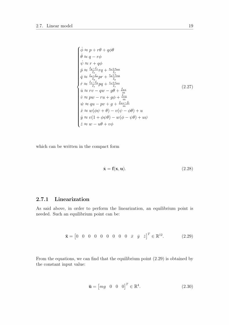
2.7. Linear model 19
φ ≈ p+ rθ + qφθ
θ ≈ q − rφψ ≈ r + qφ
p ≈ Iy−IzIx
rq + τx+τwx
Ix
q ≈ Iz−IxIy
pr + τy+τwy
Iy
r ≈ Ix−IyIz
pq + τz+τwz
Iz
u ≈ rv − qw − gθ + fwx
m
v ≈ pw − ru+ gφ+ fwy
m
w ≈ qu− pv + g + fwz−ftm
x ≈ w(φψ + θ)− v(ψ − φθ) + u
y ≈ v(1 + φψθ)− w(φ− ψθ) + uψ
z ≈ w − uθ + vφ
(2.27)
which can be written in the compact form
x = f(x,u). (2.28)
2.7.1 Linearization
As said above, in order to perform the linearization, an equilibrium point isneeded. Such an equilibrium point can be:
x =[0 0 0 0 0 0 0 0 0 x y z
]T ∈ R12. (2.29)
From the equations, we can find that the equilibrium point (2.29) is obtained bythe constant input value:
u =[mg 0 0 0
]T ∈ R4. (2.30)
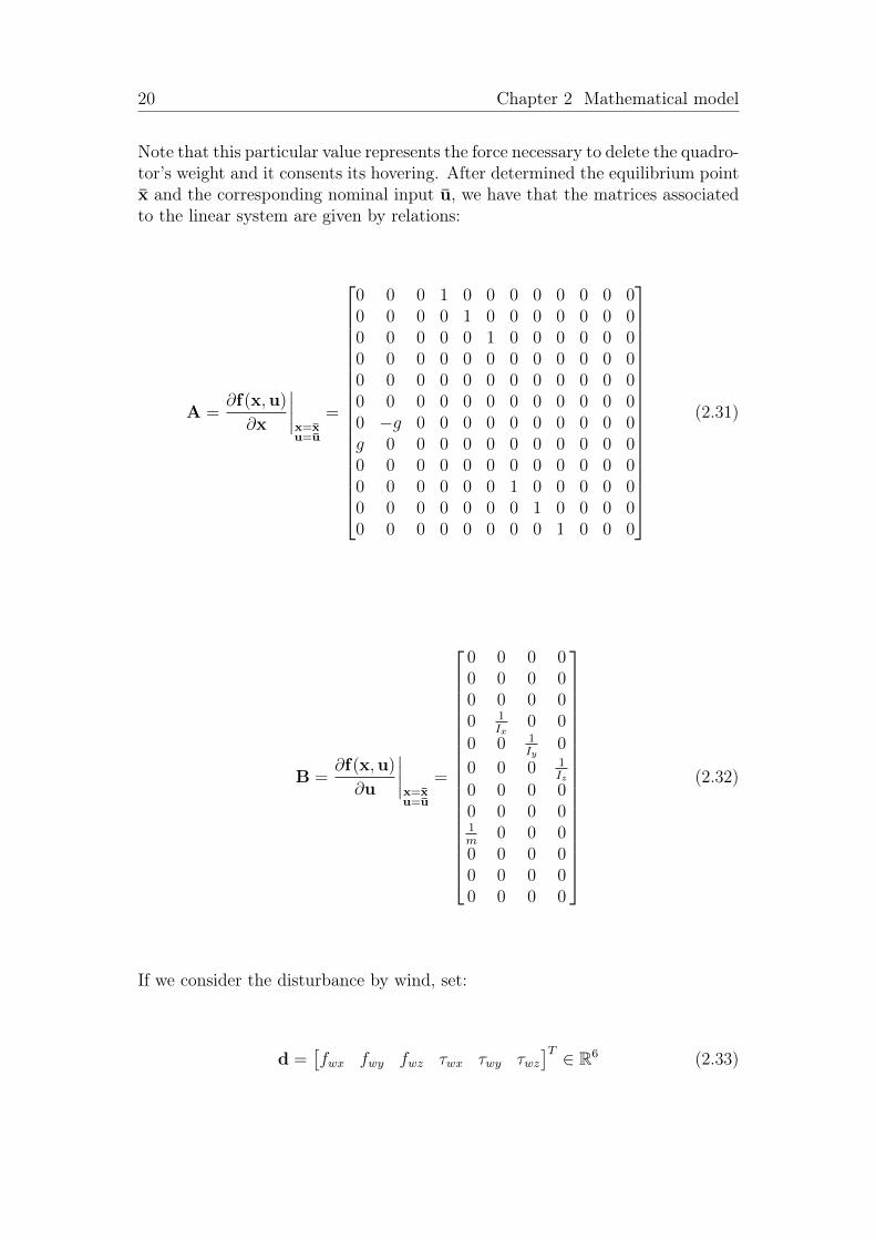
20 Chapter 2 Mathematical model
Note that this particular value represents the force necessary to delete the quadro-tor’s weight and it consents its hovering. After determined the equilibrium pointx and the corresponding nominal input u, we have that the matrices associatedto the linear system are given by relations:
A =∂f(x,u)
∂x
∣∣∣∣x=xu=u
=
0 0 0 1 0 0 0 0 0 0 0 00 0 0 0 1 0 0 0 0 0 0 00 0 0 0 0 1 0 0 0 0 0 00 0 0 0 0 0 0 0 0 0 0 00 0 0 0 0 0 0 0 0 0 0 00 0 0 0 0 0 0 0 0 0 0 00 −g 0 0 0 0 0 0 0 0 0 0g 0 0 0 0 0 0 0 0 0 0 00 0 0 0 0 0 0 0 0 0 0 00 0 0 0 0 0 1 0 0 0 0 00 0 0 0 0 0 0 1 0 0 0 00 0 0 0 0 0 0 0 1 0 0 0
(2.31)
B =∂f(x,u)
∂u
∣∣∣∣x=xu=u
=
0 0 0 00 0 0 00 0 0 00 1
Ix0 0
0 0 1Iy
0
0 0 0 1Iz
0 0 0 00 0 0 01m
0 0 00 0 0 00 0 0 00 0 0 0
(2.32)
If we consider the disturbance by wind, set:
d =[fwx fwy fwz τwx τwy τwz
]T ∈ R6 (2.33)
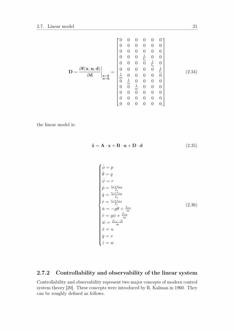
2.7. Linear model 21
D =∂f(x,u,d)
∂d
∣∣∣∣x=xu=u
=
0 0 0 0 0 00 0 0 0 0 00 0 0 0 0 00 0 0 1
Ix0 0
0 0 0 0 1Iy
0
0 0 0 0 0 1Iz
1m
0 0 0 0 00 1
m0 0 0 0
0 0 1m
0 0 00 0 0 0 0 00 0 0 0 0 00 0 0 0 0 0
(2.34)
the linear model is:
x = A · x + B · u + D · d (2.35)
φ = p
θ = q
ψ = r
p = τx+τwx
Ix
q = τy+τwy
Iy
r = τz+τwz
Iz
u = −gθ + fwx
m
v = gφ+ fwy
m
w = fwz−ftm
x = u
y = v
z = w
(2.36)
2.7.2 Controllability and observability of the linear system
Controllability and observability represent two major concepts of modern controlsystem theory [20]. These concepts were introduced by R. Kalman in 1960. Theycan be roughly defined as follows.
22 Chapter 2 Mathematical model
• Controllability: In order to be able to do whatever we want with the givendynamic system under control input, the system must be controllable.
• Observability: In order to see what is going on inside the system, thesystem must be observable.
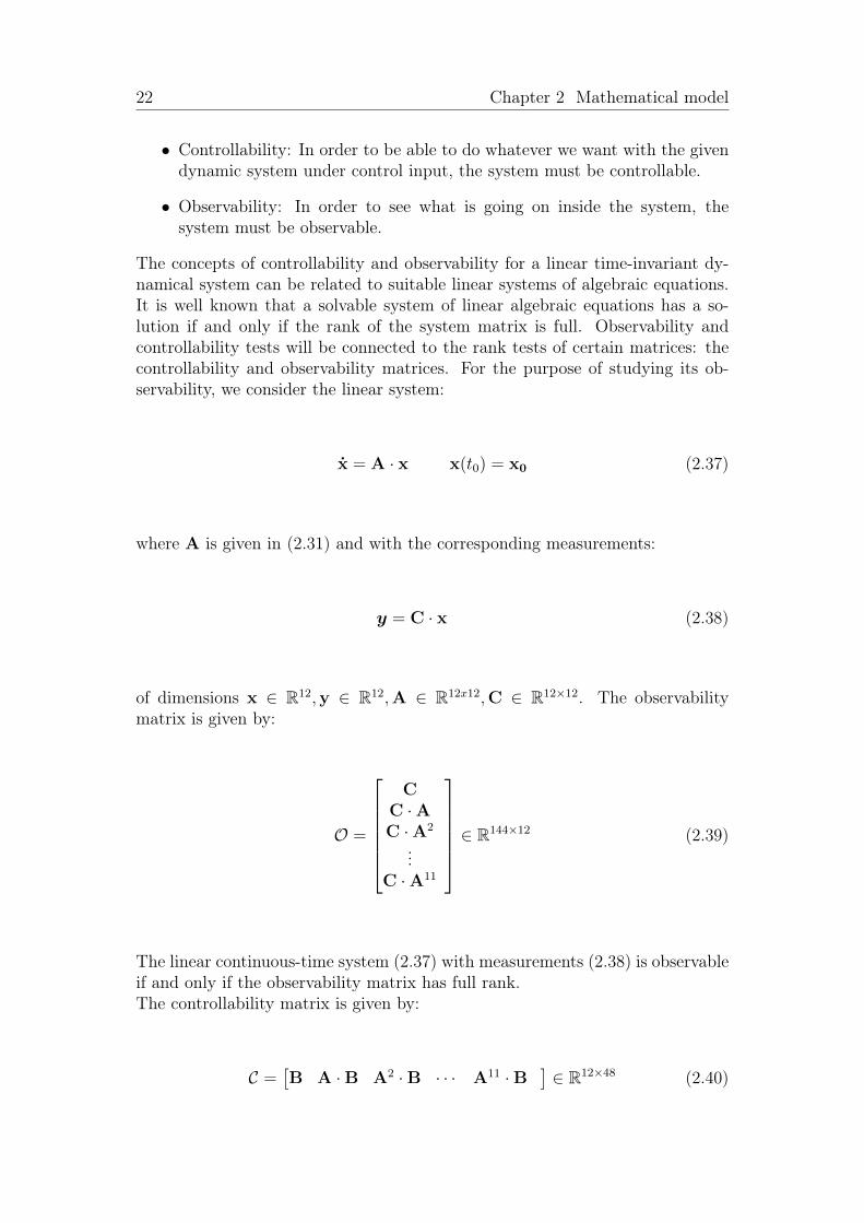
The concepts of controllability and observability for a linear time-invariant dy-namical system can be related to suitable linear systems of algebraic equations.It is well known that a solvable system of linear algebraic equations has a so-lution if and only if the rank of the system matrix is full. Observability andcontrollability tests will be connected to the rank tests of certain matrices: thecontrollability and observability matrices. For the purpose of studying its ob-servability, we consider the linear system:
x = A · x x(t0) = x0 (2.37)
where A is given in (2.31) and with the corresponding measurements:
y = C · x (2.38)
of dimensions x ∈ R12,y ∈ R12,A ∈ R12x12,C ∈ R12×12. The observabilitymatrix is given by:
O =
CC ·AC ·A2
...C ·A11
∈ R144×12 (2.39)
The linear continuous-time system (2.37) with measurements (2.38) is observableif and only if the observability matrix has full rank.The controllability matrix is given by:
C =[B A ·B A2 ·B · · · A11 ·B
]∈ R12×48 (2.40)

2.7. Linear model 23
where B is given in (2.32). The linear continuous-time system (2.37) with mea-surements (2.38) is controllable if and only if the controllability matrix has fullrank. To check its observability and controllability, we used Matlab. The linearsystem results to be controllable and observable.

24 Chapter 2 Mathematical model
Chapter 3
Control strategies
In this section we discuss three control strategies. One control strategy is linear(Linear Quadratic Regulator), and the other two control strategies are nonlin-ear (exact linearization and non-interacting control via dynamic feedback anddynamic inversion with zero-dynamics stabilization). Some comparisons aboutthese control strategies are done.
3.1 Linear Quadratic Regulator controlThe objective of the optimal control [30] is to determine control signal so that thesystem to be controlled can meet physical constraints and minimize/maximize acost/performance function. Namely, the solution of an optimization problem issupposed to bring the system’s state x(t) to the desired trajectory xd minimizingsome cost. Furthermore, it minimize the use of the control inputs, thus reducingthe use of actuators.
The underling needs of optimization control are:
• A model able to best describe the behavior of the dynamic system targetof control;
• A cost index J , taking into account specifications and need of the designer;
• Possible boundary conditions and physical constraints limiting the system.
Let us consider a dynamic system and set x as state and set u as input:
x(t) = f [x(t),u(t), t]. (3.1)
Being x and u vectors of n− 1 and r − 1 length, it is possible to define J as:
25
26 Chapter 3 Control strategies
J = e[x(tf )] +
∫ tf
t0
w[x(t),u(t), t]dt, (3.2)
where the weight function w and the terminal cost e are non-negative functionsuch as w(0,0, t) = 0 and e(0) = 0. The boundary conditions are:
• x(t0) = x0 ;
• x(tf ) and tf unconstrained.
It is then possible to define the solution of an optimization problem:
u(t),∀t ∈ [t0, tf ]. (3.3)
Such a function aims at minimizing J . Considering the limit of the time intervalas approaching infinitive, highlighting the system and the cost index:
x = A · x + B · uy = C · x (3.4)
J =
∫ ∞
t0
u(t)T ·R · u(t) + [x(t)− xd(t)]T ·Q · [x(t)− xd(t)]dt, (3.5)
being R and Q such matrixes that:
• R is the cost of actuators (R = RT positive definite matrix; R ∈ Rm×m);
• Q is the cost of the state (Q = QT positive semi-definite matrix; Q ∈ Rr×r).
It is possible to demonstrate [30] that the control’s input u(·) which minimizesthe functional is a state linear feedback as:
u(t) = −K · [x(t)− xd(t)], (3.6)
3.1. Linear Quadratic Regulator control 27
where:
K = R−1 ·BT · S. (3.7)
The S matrix is a solution of the Riccati’s algebraic equation:
S ·A + AT · S− S ·BR−1 ·BT · S + CT ·Q ·C = 0, (3.8)
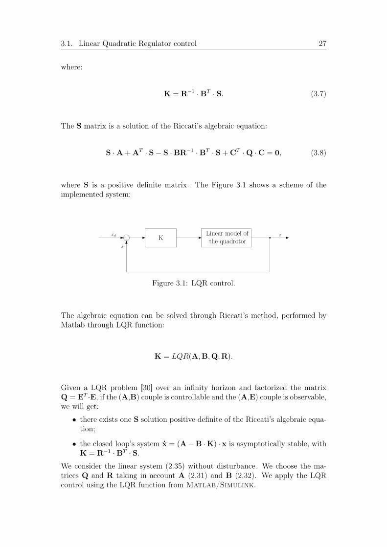
where S is a positive definite matrix. The Figure 3.1 shows a scheme of theimplemented system:
Linear model ofthe quadrotor
Kx
xd x
Figure 3.1: LQR control.
The algebraic equation can be solved through Riccati’s method, performed byMatlab through LQR function:
K = LQR(A,B,Q,R).
Given a LQR problem [30] over an infinity horizon and factorized the matrixQ = ET ·E, if the (A,B) couple is controllable and the (A,E) couple is observable,we will get:
• there exists one S solution positive definite of the Riccati’s algebraic equa-tion;
• the closed loop’s system x = (A−B ·K) · x is asymptotically stable, withK = R−1 ·BT · S.
We consider the linear system (2.35) without disturbance. We choose the ma-trices Q and R taking in account A (2.31) and B (2.32). We apply the LQRcontrol using the LQR function from Matlab/Simulink.
28 Chapter 3 Control strategies
3.2 Feedback linearization controlFeedback linearization is an approach to nonlinear control design [28] that hasattracted several researches in the last years. The central idea is to algebraicallytransform nonlinear systems dynamics into (fully or partly) linear ones, so thatlinear control techniques can be applied. Two nonlinear control design techniquesare discussed here in detail.In this chapter, we will focus on continuous-time, state-space models of the form
x = f(x) + G(x) · uy = h(x)
(3.9)
where: x ∈ Rn is the vector of state variables, u ∈ Rm is the vector of controlinput variables, y ∈ Rm is the vector of output variables, f(x) is an n-dimensionalvector of nonlinear functions, G(x) is an (n×m)-dimensional matrix of nonlinearfunctions and h(x) is anm-dimensional vector of nonlinear functions. The single-input, single-output (SISO) case where m = 1 will be emphasized to explain thebasic concepts.Consider the Jacobian linearization 2.7.1 of the nonlinear model (3.9) aroundan equilibrium point (u0,x0,y0). In this way the model can be written as alinearized state-space system,
x = A · x + B · uy = C · x (3.10)
with obvious definition for the matrices A,B,C. It is important to note that(3.2) is an exact representation of nonlinear model only at the point (x0,u0). Asa result, a control strategy based on a linearized model may yield unsatisfactoyperformance and robustness at other operating points.In this section we show that this kind of nonlinear control techniques can producea linear model that is an exact representation of the original nonlinear model overa large set of operating conditions. The feedback linearization is based on twooperations:
• nonlinear change of coordinates;
• nonlinear state feedback.
After the feedback linearization, the input-output model is linear in the new setof coordinates. Specifically, we have:
3.2. Feedback linearization control 29
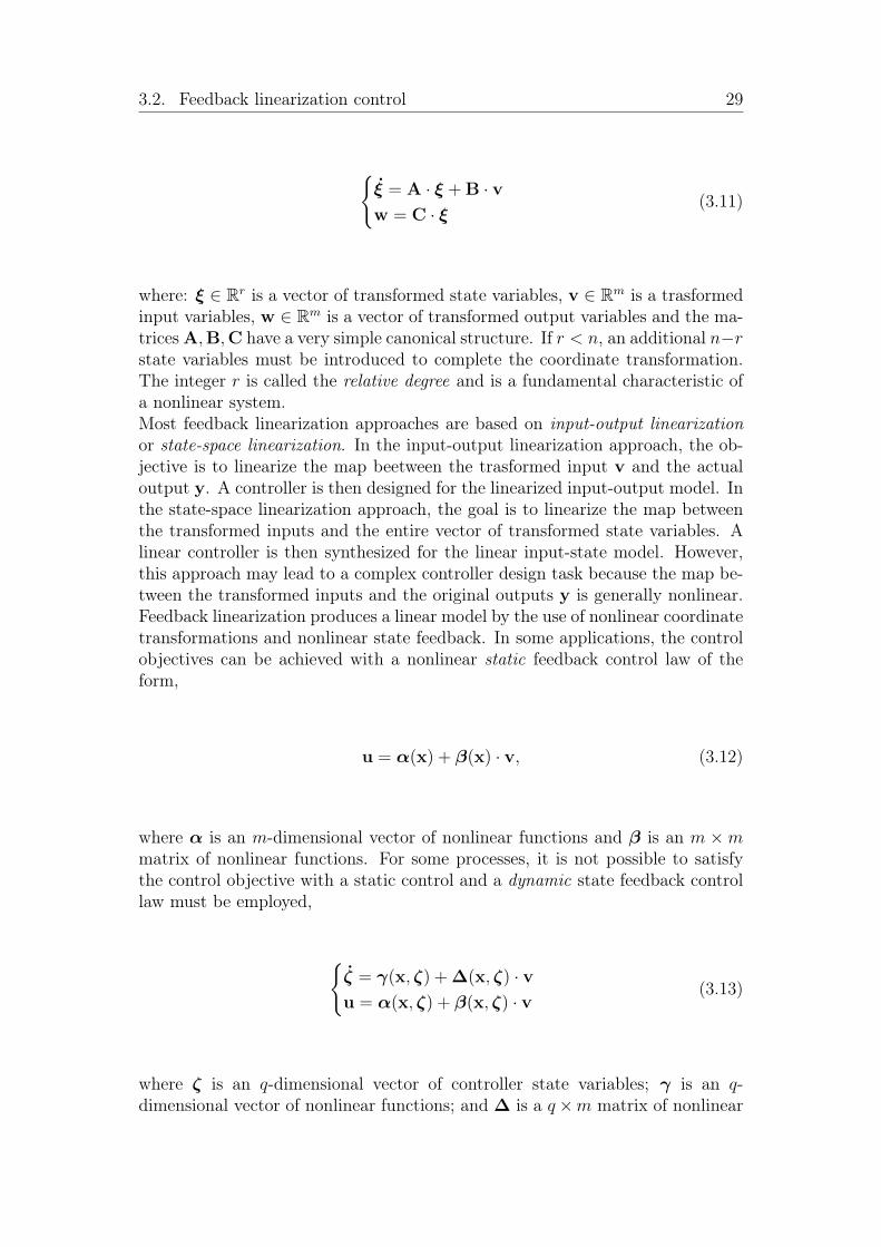
ξ = A · ξ + B · vw = C · ξ (3.11)
where: ξ ∈ Rr is a vector of transformed state variables, v ∈ Rm is a trasformedinput variables, w ∈ Rm is a vector of transformed output variables and the ma-trices A,B,C have a very simple canonical structure. If r < n, an additional n−rstate variables must be introduced to complete the coordinate transformation.The integer r is called the relative degree and is a fundamental characteristic ofa nonlinear system.Most feedback linearization approaches are based on input-output linearizationor state-space linearization. In the input-output linearization approach, the ob-jective is to linearize the map beetween the trasformed input v and the actualoutput y. A controller is then designed for the linearized input-output model. Inthe state-space linearization approach, the goal is to linearize the map betweenthe transformed inputs and the entire vector of transformed state variables. Alinear controller is then synthesized for the linear input-state model. However,this approach may lead to a complex controller design task because the map be-tween the transformed inputs and the original outputs y is generally nonlinear.Feedback linearization produces a linear model by the use of nonlinear coordinatetransformations and nonlinear state feedback. In some applications, the controlobjectives can be achieved with a nonlinear static feedback control law of theform,
u = α(x) + β(x) · v, (3.12)
where α is an m-dimensional vector of nonlinear functions and β is an m ×mmatrix of nonlinear functions. For some processes, it is not possible to satisfythe control objective with a static control and a dynamic state feedback controllaw must be employed,
ζ = γ(x, ζ) + ∆(x, ζ) · vu = α(x, ζ) + β(x, ζ) · v (3.13)
where ζ is an q-dimensional vector of controller state variables; γ is an q-dimensional vector of nonlinear functions; and ∆ is a q×m matrix of nonlinear
30 Chapter 3 Control strategies
functions.The quadrotor has six outputs y =
[x y z φ θ ψ
]and the vehicle has four
inputs. There are two degree of freedom that are left uncontrollable. A solutionto this problem [11] is to decompose it into two distinct control loops (Dynamicinversion with zero-dynamics stabilization). Another solution provides the useof dynamic feedback control (Exact linearization and non-interacting control viadynamic feedback). Such control structures are based on the input-output lin-earization described in appendix A.
3.2.1 Exact linearization and non-interacting control viadynamic feedback
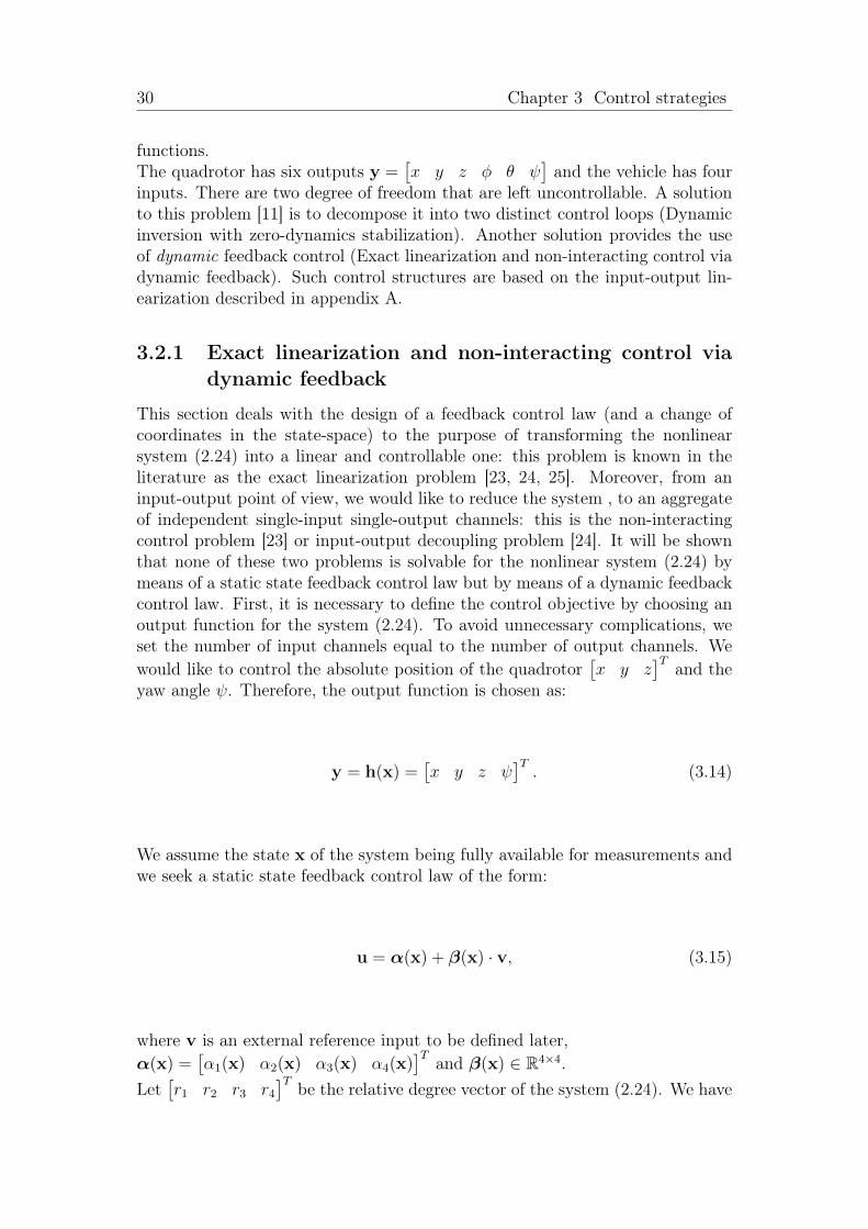
This section deals with the design of a feedback control law (and a change ofcoordinates in the state-space) to the purpose of transforming the nonlinearsystem (2.24) into a linear and controllable one: this problem is known in theliterature as the exact linearization problem [23, 24, 25]. Moreover, from aninput-output point of view, we would like to reduce the system , to an aggregateof independent single-input single-output channels: this is the non-interactingcontrol problem [23] or input-output decoupling problem [24]. It will be shownthat none of these two problems is solvable for the nonlinear system (2.24) bymeans of a static state feedback control law but by means of a dynamic feedbackcontrol law. First, it is necessary to define the control objective by choosing anoutput function for the system (2.24). To avoid unnecessary complications, weset the number of input channels equal to the number of output channels. Wewould like to control the absolute position of the quadrotor
[x y z
]T and theyaw angle ψ. Therefore, the output function is chosen as:
y = h(x) =[x y z ψ
]T. (3.14)
We assume the state x of the system being fully available for measurements andwe seek a static state feedback control law of the form:
u = α(x) + β(x) · v, (3.15)
where v is an external reference input to be defined later,α(x) =
[α1(x) α2(x) α3(x) α4(x)
]T and β(x) ∈ R4×4.Let
[r1 r2 r3 r4
]T be the relative degree vector of the system (2.24). We have
3.2. Feedback linearization control 31
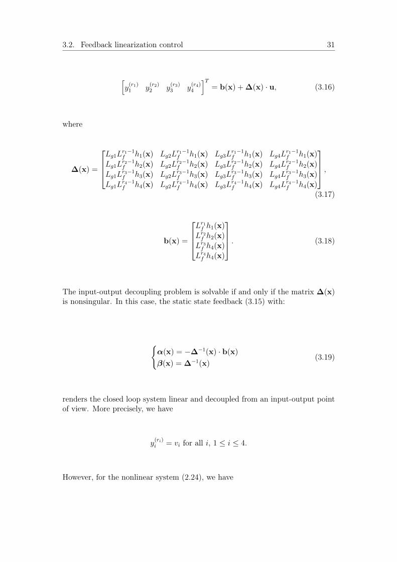
[y(r1)1 y
(r2)2 y
(r3)3 y
(r4)4
]T= b(x) + ∆(x) · u, (3.16)
where
∆(x) =
Lg1Lr1−1f h1(x) Lg2L
r1−1f h1(x) Lg3L
r1−1f h1(x) Lg4L
r1−1f h1(x)
Lg1Lr2−1f h2(x) Lg2L
r2−1f h2(x) Lg3L
r2−1f h2(x) Lg4L
r2−1f h2(x)
Lg1Lr3−1f h3(x) Lg2L
r3−1f h3(x) Lg3L
r3−1f h3(x) Lg4L
r3−1f h3(x)
Lg1Lr4−1f h4(x) Lg2L
r4−1f h4(x) Lg3L
r4−1f h4(x) Lg4L
r4−1f h4(x)
,
(3.17)
b(x) =
Lr1f h1(x)
Lr2f h2(x)
Lr3f h4(x)
Lr4f h4(x)
. (3.18)
The input-output decoupling problem is solvable if and only if the matrix ∆(x)is nonsingular. In this case, the static state feedback (3.15) with:
α(x) = −∆−1(x) · b(x)
β(x) = ∆−1(x)(3.19)
renders the closed loop system linear and decoupled from an input-output pointof view. More precisely, we have
y(ri)i = vi for all i, 1 ≤ i ≤ 4.
However, for the nonlinear system (2.24), we have
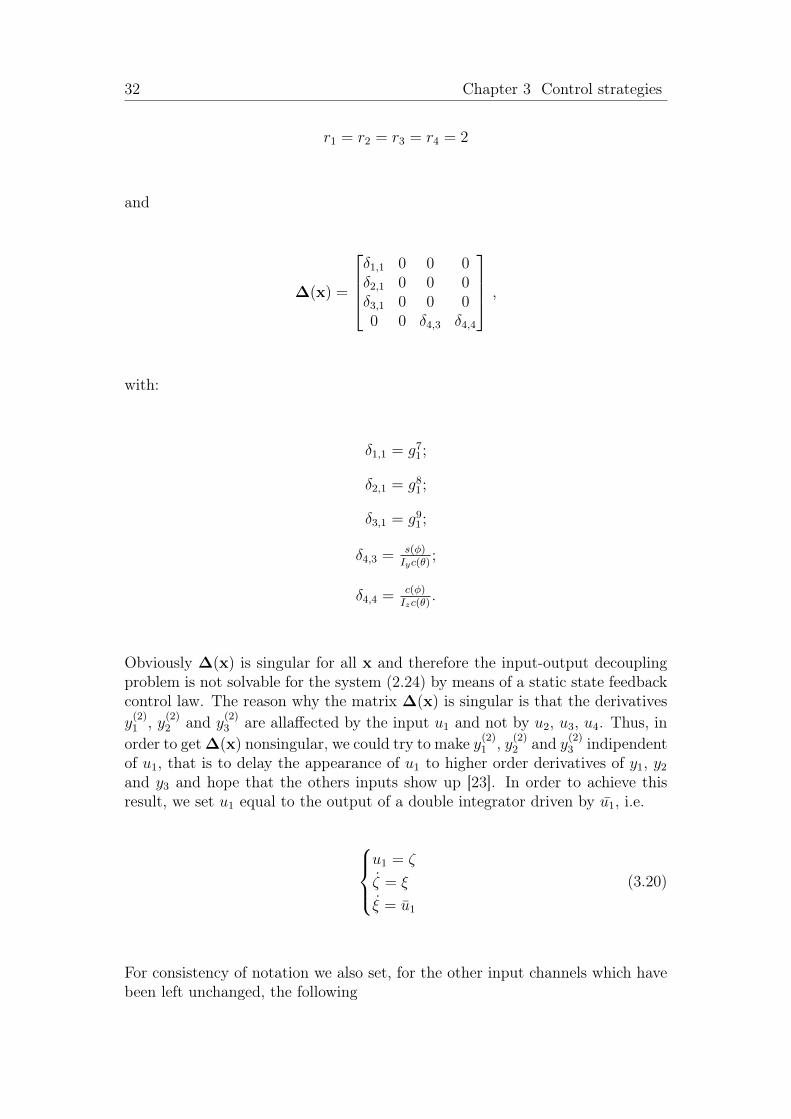
32 Chapter 3 Control strategies
r1 = r2 = r3 = r4 = 2
and
∆(x) =
δ1,1 0 0 0δ2,1 0 0 0δ3,1 0 0 00 0 δ4,3 δ4,4
,
with:
δ1,1 = g71;
δ2,1 = g81;
δ3,1 = g91;
δ4,3 = s(φ)Iyc(θ)
;
δ4,4 = c(φ)Izc(θ)
.
Obviously ∆(x) is singular for all x and therefore the input-output decouplingproblem is not solvable for the system (2.24) by means of a static state feedbackcontrol law. The reason why the matrix ∆(x) is singular is that the derivativesy(2)1 , y(2)2 and y(2)3 are allaffected by the input u1 and not by u2, u3, u4. Thus, inorder to get ∆(x) nonsingular, we could try to make y(2)1 , y(2)2 and y(2)3 indipendentof u1, that is to delay the appearance of u1 to higher order derivatives of y1, y2and y3 and hope that the others inputs show up [23]. In order to achieve thisresult, we set u1 equal to the output of a double integrator driven by u1, i.e.
u1 = ζ
ζ = ξ
ξ = u1
(3.20)
For consistency of notation we also set, for the other input channels which havebeen left unchanged, the following
3.2. Feedback linearization control 33
u2 = u2
u3 = u3
u4 = u4
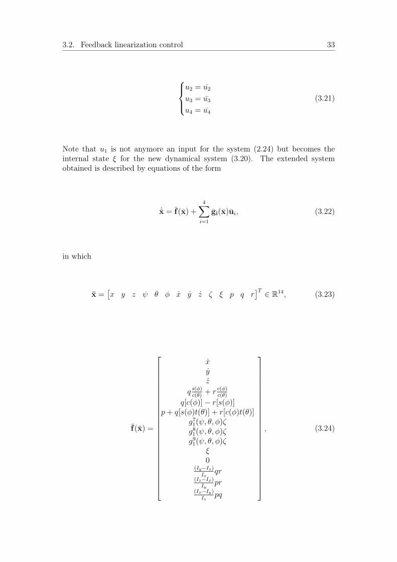
(3.21)
Note that u1 is not anymore an input for the system (2.24) but becomes theinternal state ξ for the new dynamical system (3.20). The extended systemobtained is described by equations of the form
˙x = f(x) +4∑
i=1
gi(x)ui, (3.22)
in which
x =[x y z ψ θ φ x y z ζ ξ p q r
]T ∈ R14, (3.23)
f(x) =
xyz
q s(φ)c(θ)
+ r c(φ)c(θ)
q[c(φ)]− r[s(φ)]p+ q[s(φ)t(θ)] + r[c(φ)t(θ)]
g71(ψ, θ, φ)ζg81(ψ, θ, φ)ζg91(ψ, θ, φ)ζ
ξ0
(Iy−Iz)Ix
qr(Iz−Ix)Iy
pr(Ix−Iy)Iz
pq
, (3.24)
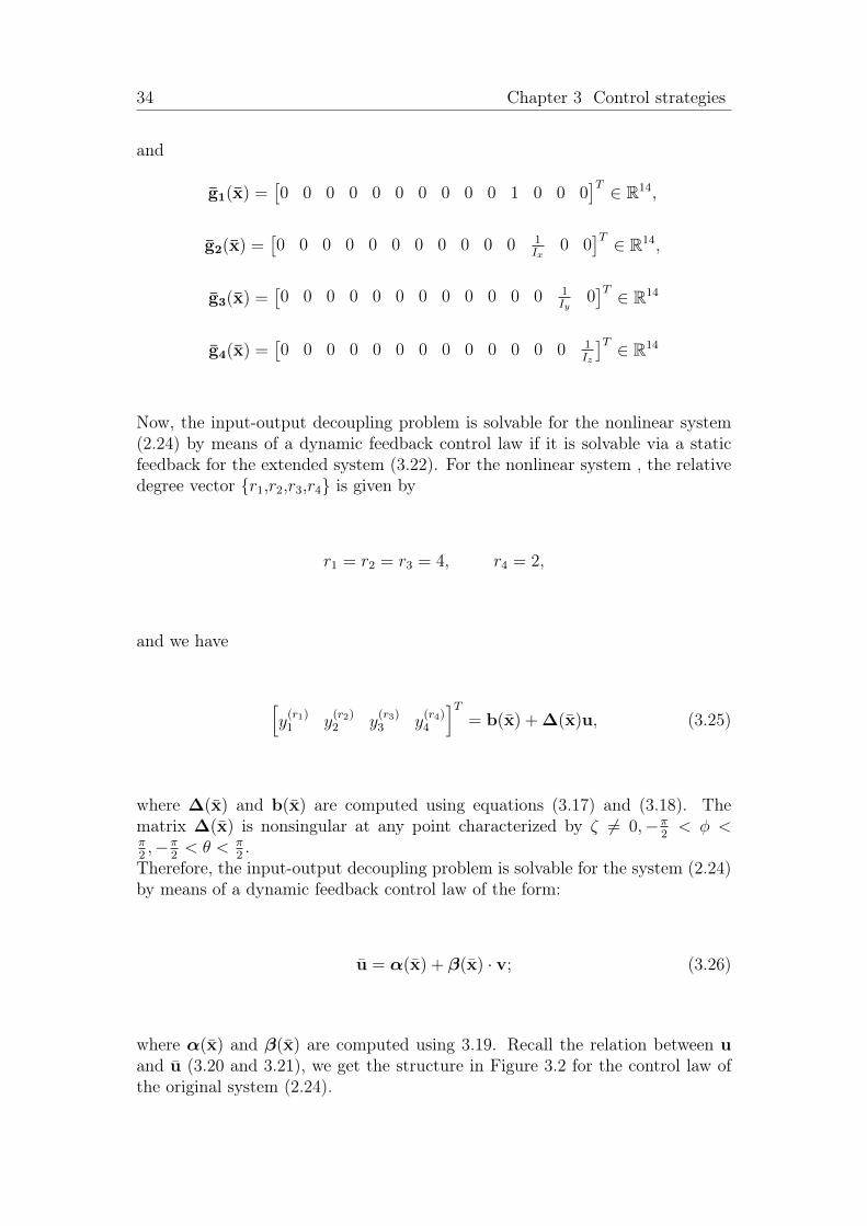
34 Chapter 3 Control strategies
and
g1(x) =[0 0 0 0 0 0 0 0 0 0 1 0 0 0
]T ∈ R14,
g2(x) =[0 0 0 0 0 0 0 0 0 0 0 1
Ix0 0
]T ∈ R14,
g3(x) =[0 0 0 0 0 0 0 0 0 0 0 0 1
Iy0]T ∈ R14
g4(x) =[0 0 0 0 0 0 0 0 0 0 0 0 0 1
Iz
]T ∈ R14
Now, the input-output decoupling problem is solvable for the nonlinear system(2.24) by means of a dynamic feedback control law if it is solvable via a staticfeedback for the extended system (3.22). For the nonlinear system , the relativedegree vector r1,r2,r3,r4 is given by
r1 = r2 = r3 = 4, r4 = 2,
and we have
[y(r1)1 y
(r2)2 y
(r3)3 y
(r4)4
]T= b(x) + ∆(x)u, (3.25)
where ∆(x) and b(x) are computed using equations (3.17) and (3.18). Thematrix ∆(x) is nonsingular at any point characterized by ζ 6= 0,−π
2< φ <
π2,−π
2< θ < π
2.
Therefore, the input-output decoupling problem is solvable for the system (2.24)by means of a dynamic feedback control law of the form:
u = α(x) + β(x) · v; (3.26)
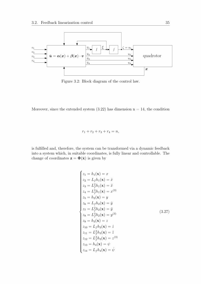
where α(x) and β(x) are computed using 3.19. Recall the relation between uand u (3.20 and 3.21), we get the structure in Figure 3.2 for the control law ofthe original system (2.24).
3.2. Feedback linearization control 35
∫ ∫v1v2v3v4
u1
u2
u3
u4
quadrotoru = α(x ) + β(x ) · v
x
ξ ζ = u1
u2
u3
u4
Figure 3.2: Block diagram of the control law.
Moreover, since the extended system (3.22) has dimension n = 14, the condition
r1 + r2 + r3 + r4 = n,
is fulfilled and, therefore, the system can be transformed via a dynamic feedbackinto a system which, in suitable coordinates, is fully linear and controllable. Thechange of coordinates z = Φ(x) is given by
z1 = h1(x) = x
z2 = Lfh1(x) = x
z3 = L2fh1(x) = x
z4 = L3fh1(x) = x(3)
z5 = h2(x) = y
z6 = Lfh2(x) = y
z7 = L2fh2(x) = y
z8 = L3fh2(x) = y(3)
z9 = h3(x) = z
z10 = Lfh3(x) = z
z11 = L2fh3(x) = z
z12 = L3fh3(x) = z(3)
z13 = h4(x) = ψ
z14 = Lfh4(x) = ψ
(3.27)
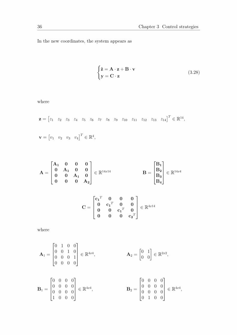
36 Chapter 3 Control strategies
In the new coordinates, the system appears as
z = A · z + B · vy = C · z (3.28)
where
z =[z1 z2 z3 z4 z5 z6 z7 z8 z9 z10 z11 z12 z13 z14
]T ∈ R14,
v =[v1 v2 v3 v4
]T ∈ R4,
A =
A1 0 0 00 A1 0 00 0 A1 00 0 0 A2
∈ R14x14 B =
B1
B2
B3
B4
∈ R14x4
C =
c1T 0 0 0
0 c1T 0 0
0 0 c1T 0
0 0 0 c2T
∈ R4x14
where
A1 =
0 1 0 00 0 1 00 0 0 10 0 0 0
∈ R4x4, A2 =
[0 10 0
]∈ R2x2,
B1 =
0 0 0 00 0 0 00 0 0 01 0 0 0
∈ R4x4, B2 =
0 0 0 00 0 0 00 0 0 00 1 0 0
∈ R4x4,
3.2. Feedback linearization control 37
B3 =
0 0 0 00 0 0 00 0 0 00 0 1 0
∈ R4x4, B4 =
[0 0 0 00 0 0 0
]∈ R2x4,
c1 =[1 0 0 0
]T ∈ R4, c2 =[1 0
]T ∈ R2,
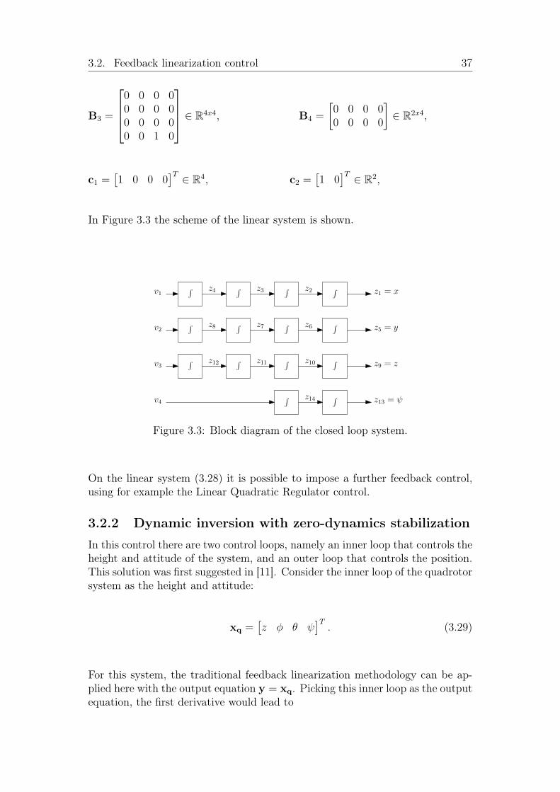
In Figure 3.3 the scheme of the linear system is shown.
∫ ∫v1
v2
v3
v4
∫∫
∫ ∫ ∫ ∫
∫ ∫ ∫ ∫
∫ ∫
z1 = xz2z3z4
z5 = yz6z7z8
z9 = zz10z11z12
z13 = ψz14
Figure 3.3: Block diagram of the closed loop system.
On the linear system (3.28) it is possible to impose a further feedback control,using for example the Linear Quadratic Regulator control.
3.2.2 Dynamic inversion with zero-dynamics stabilization
In this control there are two control loops, namely an inner loop that controls theheight and attitude of the system, and an outer loop that controls the position.This solution was first suggested in [11]. Consider the inner loop of the quadrotorsystem as the height and attitude:
xq =[z φ θ ψ
]T. (3.29)
For this system, the traditional feedback linearization methodology can be ap-plied here with the output equation y = xq. Picking this inner loop as the outputequation, the first derivative would lead to
38 Chapter 3 Control strategies
xq =[z φ θ ψ
]T. (3.30)
Note here that the control input dependent term Lgh(x) is zero. Consider thesubsystem of the (2.22), it appear as,
xq =
z
φ
θ
ψ
= b(x) + ∆(x) · u, (3.31)
where
b(x) =
g
θψ Iy−IxIx
φψ Iz−IxIy
φθ Ix−IyIz
, (3.32)
∆(x) =
− 1mcθcφ 0 0 00 1
Ix0 0
0 0 1Iy
0 0 0 1Iy
, (3.33)
u =
ftτxτyτz
, (3.34)
A simplification is made by setting[φ θ ψ
]=[p q r
]. The assumption holds
for smaller angles of movement. Based on the dynamics described in (3.31), thecontrol input can be selected as (A.8) to be
u = α(x) + β(x) · v. (3.35)
3.2. Feedback linearization control 39
with
α(x) = −∆−1(x) · b(x)
β(x) = ∆−1(x)(3.36)
The remaining linear dynamics after feedback linearization are an integratorchain, xq = v, which can be controlled by the linear controller:
v = xdq −Kv · (xq − xd
q)−Kp · (xq − xdq), (3.37)
where, xdq is the desired acceleration of the inner loop, xd
q and xdq are the desired
trajectories for the position and their velocities. Finally, Kv and Kp, positivedefinite matrix, are tunable gains that can be used to place the poles of thesubsequent feedback linearized dynamics on the left hand side plane. Usingthe controller described in (3.35) and (3.37) the attitude of the controller canbe stabilized. However, the zero dynamics (internal states x, y), namely statesthat are not observable from the output of the previous subsystem still remainuncontrolled. These dynamics according to (2.22) are:
x = − u
m[s(φ)s(ψ) + c(φ)c(ψ)s(θ)]
y = um
[c(ψ)s(φ)− c(φ)s(ψ)s(θ)](3.38)
Das et al. [11] suggests a method to control these dynamics by controlling thedesired roll θd and pitch angle φd shown in (3.37) as part of xd
q. It consistabout two simplifying assumptions: small oscillations and to impose ψ = 0.Consequently we obtain the following simplified system:
x = − u
mθ
y = umφ
(3.39)
As before, there is a chain of two integrators to get to the desired positionvariables (x, y). Therefore, the same linear controller used in the inner loopcontrol is applied to stabilize the outer loop dynamics,
40 Chapter 3 Control strategies
θd = −m
u[xd + k11(xd − x) + k12(xd − x)]
φd = mu
[yd + k11(yd − y) + k12(yd − y)](3.40)
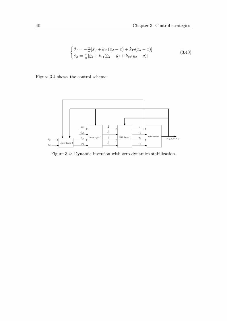
Figure 3.4 shows the control scheme:
xd
ydφd
θd
ψd
zd z
φ
θ
ψ
u
τφ
τθ
τψOuter layer 3
Inner layer 2 FBL layer 1quadorotor
x, y, z, φ, θ, ψ
Figure 3.4: Dynamic inversion with zero-dynamics stabilization.
Chapter 4
Simulation results
In this chapter we show the results obtained with Matlab/Simulink and weanalyze the differences between the several controllers illustrated above. Foreach control, we show the step response of the output variables x, y, z, ψ, thenwe show the double circle shape trajectory with the simulated results.
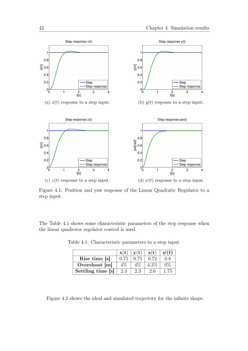
4.1 Linear Quadratic Regulator resultsFigure 4.1 shows the step response of the output variables x, y, z, ψ when theLinear Quadratic Regulator control is used.
41
42 Chapter 4 Simulation results
0 1 2 3 40
0.2
0.4
0.6
0.8
1
t[s]
x[m
]Step response x(t)
Step
Step response
(a) x(t) response to a step input.
0 1 2 3 40
0.2
0.4
0.6
0.8
1
t[s]
y[m
]
Step response y(t)
Step
Step response
(b) y(t) response to a step input.
0 1 2 3 40
0.2
0.4
0.6
0.8
1
t[s]
z[m
]
Step response z(t)
Step
Step response
(c) z(t) response to a step input.
0 1 2 3 40
0.2
0.4
0.6
0.8
1
t[s]
psi[ra
d]
Step response psi(t)
Step
Step response
(d) ψ(t) response to a step input.
Figure 4.1: Position and yaw response of the Linear Quadratic Regulator to astep input.
The Table 4.1 shows some characteristic parameters of the step response whenthe linear quadrotor regolator control is used.
Table 4.1: Characteristic parameters to a step input.
x(t) y(t) z(t) ψ(t)Rise time [s] 0.75 0.75 0.72 0.8
Overshoot [m] 4% 4% 4.3% 0%Settling time [s] 2.3 2.3 2.6 1.75
Figure 4.2 shows the ideal and simulated trajectory for the infinite shape.

4.2. Exact linearization and non-interacting control via dynamic feedbackresults 43
−3 −2 −1 0 1 2 30
1
2
3
4
x[m]
y[m
]
Trajectory 2D
Ideal trajectory
Simulated trajectory
Figure 4.2: Comparing simulated and ideal trajectory with Linear QuadraticRegulator.
In the next figures are represented the time laws for the x, y variables.
0 10 20 30−3
−2
−1
0
1
2
3
t[s]
x[m
]
Timing law x(t)
Ideal
Simulated
0 10 20 300.5
1
1.5
2
2.5
3
3.5
t[s]
y[m
]
Timing law y(t)
Figure 4.3: Ideal and simulated timing law with Linear Quadratic Regulator.
4.2 Exact linearization and non-interacting con-trol via dynamic feedback results
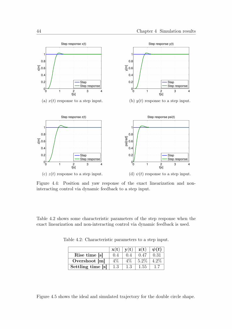
Figure 4.4 shows the step response of the output variables x, y, z, ψ when theexact linearization and non-interacting control via dynamic feedback is used.
44 Chapter 4 Simulation results
0 1 2 3 40
0.2
0.4
0.6
0.8
1
t[s]
x[m
]
Step response x(t)
Step
Step response
(a) x(t) response to a step input.
0 1 2 3 40
0.2
0.4
0.6
0.8
1
t[s]
y[m
]
Step response y(t)
Step
Step response
(b) y(t) response to a step input.
0 1 2 3 40
0.2
0.4
0.6
0.8
1
t[s]
z[m
]
Step response z(t)
Step
Step response
(c) z(t) response to a step input.
0 1 2 3 40
0.2
0.4
0.6
0.8
1
t[s]
psi[ra
d]
Step response psi(t)
Step
Step response
(d) ψ(t) response to a step input.
Figure 4.4: Position and yaw response of the exact linearization and non-interacting control via dynamic feedback to a step input.
Table 4.2 shows some characteristic parameters of the step response when theexact linearization and non-interacting control via dynamic feedback is used.
Table 4.2: Characteristic parameters to a step input.
x(t) y(t) z(t) ψ(t)Rise time [s] 0.4 0.4 0.47 0.31
Overshoot [m] 4% 4% 5.2% 4.2%Settling time [s] 1.3 1.3 1.55 1.7
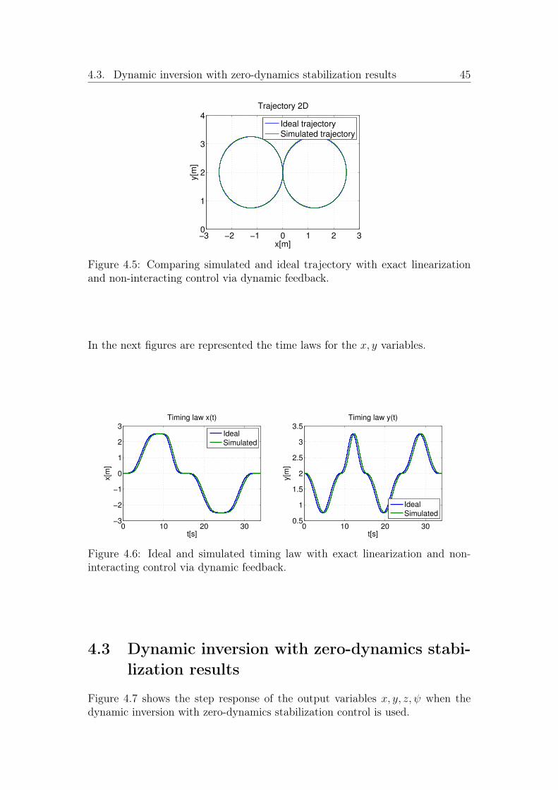
Figure 4.5 shows the ideal and simulated trajectory for the double circle shape.
4.3. Dynamic inversion with zero-dynamics stabilization results 45
−3 −2 −1 0 1 2 30
1
2
3
4
x[m]
y[m
]
Trajectory 2D
Ideal trajectory
Simulated trajectory
Figure 4.5: Comparing simulated and ideal trajectory with exact linearizationand non-interacting control via dynamic feedback.
In the next figures are represented the time laws for the x, y variables.
0 10 20 30−3
−2
−1
0
1
2
3
t[s]
x[m
]
Timing law x(t)
Ideal
Simulated
0 10 20 300.5
1
1.5
2
2.5
3
3.5
t[s]
y[m
]
Timing law y(t)
Ideal
Simulated
Figure 4.6: Ideal and simulated timing law with exact linearization and non-interacting control via dynamic feedback.
4.3 Dynamic inversion with zero-dynamics stabi-lization results
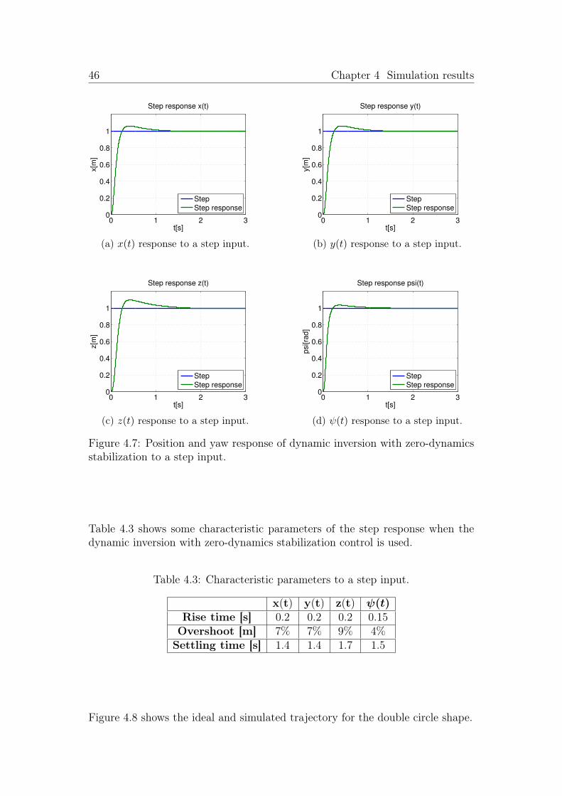
Figure 4.7 shows the step response of the output variables x, y, z, ψ when thedynamic inversion with zero-dynamics stabilization control is used.
46 Chapter 4 Simulation results
0 1 2 30
0.2
0.4
0.6
0.8
1
t[s]
x[m
]
Step response x(t)
Step
Step response
(a) x(t) response to a step input.
0 1 2 30
0.2
0.4
0.6
0.8
1
t[s]
y[m
]
Step response y(t)
Step
Step response
(b) y(t) response to a step input.
0 1 2 30
0.2
0.4
0.6
0.8
1
t[s]
z[m
]
Step response z(t)
Step
Step response
(c) z(t) response to a step input.
0 1 2 30
0.2
0.4
0.6
0.8
1
t[s]
psi[ra
d]
Step response psi(t)
Step
Step response
(d) ψ(t) response to a step input.
Figure 4.7: Position and yaw response of dynamic inversion with zero-dynamicsstabilization to a step input.
Table 4.3 shows some characteristic parameters of the step response when thedynamic inversion with zero-dynamics stabilization control is used.
Table 4.3: Characteristic parameters to a step input.
x(t) y(t) z(t) ψ(t)Rise time [s] 0.2 0.2 0.2 0.15
Overshoot [m] 7% 7% 9% 4%Settling time [s] 1.4 1.4 1.7 1.5
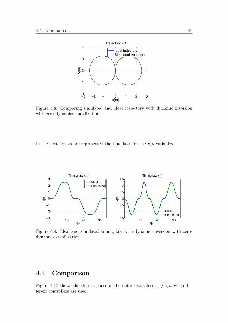
Figure 4.8 shows the ideal and simulated trajectory for the double circle shape.
4.4. Comparison 47
−3 −2 −1 0 1 2 30
1
2
3
4
x[m]
y[m
]
Trajectory 2D
Ideal trajectory
Simulated trajectory
Figure 4.8: Comparing simulated and ideal trajectory with dynamic inversionwith zero-dynamics stabilization.
In the next figures are represented the time laws for the x, y variables.
0 10 20 30−3
−2
−1
0
1
2
3
t[s]
x[m
]
Timing law x(t)
Ideal
Simulated
0 10 20 300.5
1
1.5
2
2.5
3
3.5
t[s]
y[m
]
Timing law y(t)
Ideal
Simulated
Figure 4.9: Ideal and simulated timing law with dynamic inversion with zero-dynamics stabilization.
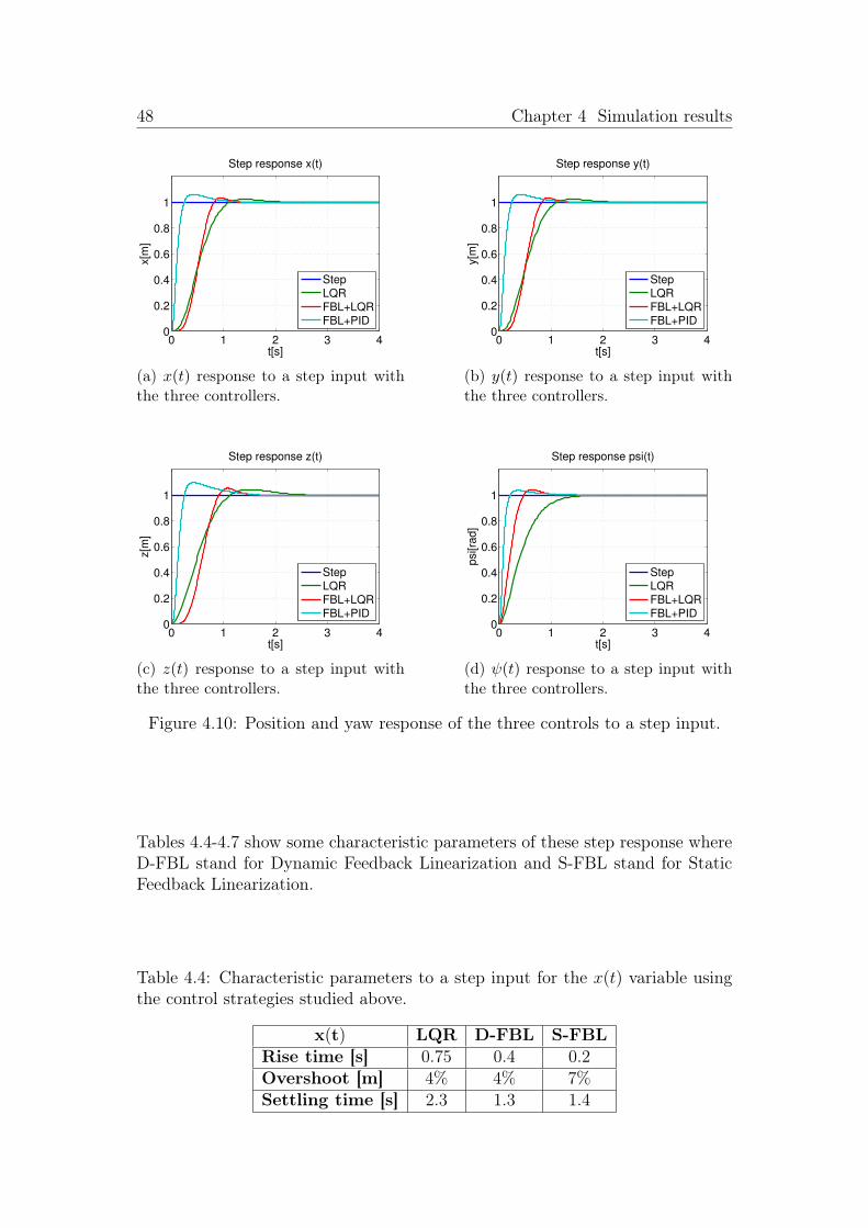
4.4 Comparison
Figure 4.10 shows the step response of the output variables x, y, z, ψ when dif-ferent controllers are used.
48 Chapter 4 Simulation results
0 1 2 3 40
0.2
0.4
0.6
0.8
1
t[s]
x[m
]
Step response x(t)
StepLQRFBL+LQRFBL+PID
(a) x(t) response to a step input withthe three controllers.
0 1 2 3 40
0.2
0.4
0.6
0.8
1
t[s]
y[m
]
Step response y(t)
StepLQRFBL+LQRFBL+PID
(b) y(t) response to a step input withthe three controllers.
0 1 2 3 40
0.2
0.4
0.6
0.8
1
t[s]
z[m
]
Step response z(t)
StepLQRFBL+LQRFBL+PID
(c) z(t) response to a step input withthe three controllers.
0 1 2 3 40
0.2
0.4
0.6
0.8
1
t[s]
psi[ra
d]
Step response psi(t)
StepLQRFBL+LQRFBL+PID
(d) ψ(t) response to a step input withthe three controllers.
Figure 4.10: Position and yaw response of the three controls to a step input.
Tables 4.4-4.7 show some characteristic parameters of these step response whereD-FBL stand for Dynamic Feedback Linearization and S-FBL stand for StaticFeedback Linearization.
Table 4.4: Characteristic parameters to a step input for the x(t) variable usingthe control strategies studied above.
x(t) LQR D-FBL S-FBLRise time [s] 0.75 0.4 0.2Overshoot [m] 4% 4% 7%Settling time [s] 2.3 1.3 1.4
4.5. 3D Animation 49
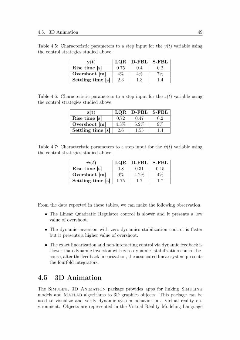
Table 4.5: Characteristic parameters to a step input for the y(t) variable usingthe control strategies studied above.
y(t) LQR D-FBL S-FBLRise time [s] 0.75 0.4 0.2Overshoot [m] 4% 4% 7%Settling time [s] 2.3 1.3 1.4
Table 4.6: Characteristic parameters to a step input for the z(t) variable usingthe control strategies studied above.
z(t) LQR D-FBL S-FBLRise time [s] 0.72 0.47 0.2Overshoot [m] 4.3% 5.2% 9%Settling time [s] 2.6 1.55 1.4
Table 4.7: Characteristic parameters to a step input for the ψ(t) variable usingthe control strategies studied above.
ψ(t) LQR D-FBL S-FBLRise time [s] 0.8 0.31 0.15Overshoot [m] 0% 4.2% 4%Settling time [s] 1.75 1.7 1.7
From the data reported in these tables, we can make the following observation.
• The Linear Quadratic Regulator control is slower and it presents a lowvalue of overshoot.
• The dynamic inversion with zero-dynamics stabilization control is fasterbut it presents a higher value of overshoot.
• The exact linearization and non-interacting control via dynamic feedback isslower than dynamic inversion with zero-dynamics stabilization control be-cause, after the feedback linearization, the associated linear system presentsthe fourfold integrators.
4.5 3D AnimationThe Simulink 3D Animation package provides apps for linking Simulinkmodels and Matlab algorithms to 3D graphics objects. This package can beused to visualize and verify dynamic system behavior in a virtual reality en-vironment. Objects are represented in the Virtual Reality Modeling Language

50 Chapter 4 Simulation results
(VRML), a standard 3D modeling language. You can animate a 3D world bychanging position, rotation, scale, and other object properties during desktop orreal-time simulation [29]. In the following link, https://youtu.be/EXZJWUDSRus,the result of the simulation in Simulink 3D Animation is shown, when thedynamic inversion with zero-dynamics stabilization control is used and the de-sired trajectory is the double circle shape. To realize the desired trajectory hasbeen used a particular Matlab script. Such Matlab script realizes the desiredtrajectory using a trapezoidal velocity profile [31].
Chapter 5
Conclusions and futuredevelopments
In this work, firstly, a mathematical model of a quadrotor dynamics is derived,using Newton’s and Euler’s laws. Then a linearized version of the model isobtained, and therefore a linear controller, the Linear Quadratic Regulator, isderived. After that, two feedback linearization control schemes are designed.The first one is the dynamic inversion with zero dynamics stabilization, basedon static feedback linearization obtaining a partial linearization of the mathe-matical model. The second one is the exact linearization and non-interactingcontrol via dynamic feedback, based on dynamic feedback linearization obtain-ing a total linearization of the mathematical model. Moreover, these nonlinearcontrol strategies are compared with the Linear Quadratic Regulator in terms ofperformances. Finally, the behavior of the quadrotor under the proposed con-trol strategies is observed in virtual reality by using the Simulink 3D Animationtoolbox. A future project could be the applying nonlinear control technique, likefeedback linearization, adaptive feedback linearization, sliding mode control, forthe real quadrotor to obtain best performance.
51

52 Chapter 5 Conclusions and future developments
Appendix A
Input-output FeedbackLinearization
Consider a system with state x ∈ Rn, input u ∈ R and output y ∈ R whosedynamics are given by
x = f(x) + g(x)u
y = h(x)(A.1)
where f , g and h are sufficiently smooth. We focus now on a single-input, single-output system, i.e., u, y ∈ R. The derivative of the output y can be expressed as[17]
y =∂h
∂x[f(x) + g(x)u]. (A.2)
The derivative of h along the trajectory of the state x is known as the LieDerivate and is denoted as [17]
y =∂h
∂x[f(x) + g(x)u] = Lfh(x) + Lgh(x)u. (A.3)
If on the first derivative Lgh(x) = 0, we have
y = y(1) = Lfh(x). (A.4)
53
54 Chapter A Input-output Feedback Linearization
Note that, in this case, the output y remains independent of input u. However,further higher order derivatives can be considered, specifically,
y(2) = L2fh(x) + LgLfh(x)u, (A.5)
y(3) = L3fh(x) + LgL
2fh(x)u, (A.6)
y(i) = Lifh(x) + LgLi−1f h(x)u, (A.7)
and if for a certain i, LgLi−1f h(x)u 6= 0, then the equation (A.7) can be linearizedwith full state feedback by,
u =1
LgLi−1f h(x)
(−Lifh(x) + v), (A.8)
in the state region where the inverse 1
LgLi−1f h(x)
exists. In this region the feedbacklinearized model becomes,
y(i) = v. (A.9)
The value i is defined to be the relative degree of the system. The resulting lineardynamic system defined in (A.9) can be stabilized by standarùd linear controltechniques and consists of a set of i− 1 integrators up to the required output y.Moreover, with this linearization a linear controller can be designed such thatthe overall system can be proven to be exponentially stable [21].The concepts used for SISO systems can be also extended to MIMO systems [22].In the MIMO case, we consider square systems (that is systems with the samenumber of inputs and outputs) of the form,
x = f(x) + G(x) · uy = h(x)
, (A.10)
55
where x ∈ Rn is a state vector, u ∈ Rm is a control input vector (of componentsui), y ∈ Rm is a vector of system output (of components yi), f , h are smoothvector fields, and G in an n×m matrix whose columns are smooth vector fieldsgi. Input-output linearization of MIMO systems is obtained similarly to theSISO case, by differentiating the outputs yi until the inputs appear. Assumethat ri is the smallest integer such that at least one of the inputs appears in y(ri)i
then,
y(ri)i = Lrif hi(x) +
m∑
j=1
LgjLri−1f hi(x)uj, (A.11)
with LgjLri−1f hi(x) 6= 0 for some x. Performing the above procedure for each
output yi yields
y(r1)1...
y(rm)m
=
Lr1f h1(x)
...Lrmf hm(x)
+ E(x)u, (A.12)
where the mxm matrix E(x) is defined obviously. If E(x) is invertible for all x,then, similarly to the SISO case, the input transformation
u = −E−1 ·
Lr1f h1(x)
...Lrmf hm(x)
, (A.13)
yields m equations of the simple form
y(ri)i = vi. (A.14)
Since the input vi only affects the output yi, (A.13) is called a decoupling controllaw, and the invertible matrix E(x) is called decoupling matrix of the system.The system (A.10), is then said to have relative degree (r1, ...., rm), and the scalar
56 Chapter A Input-output Feedback Linearization
r = r1 + ...+ rm is called the total relative degree of the system.An interesting case corresponds to the total relative degree being n. In this case,there are no internal dynamics. With the control law in the form of (A.13), wethus obtain an input-state linearization of the original nonlinear system. Withthe equivalent inputs vi designed as in the SISO case, both stabilization andtracking can then be achieved for the system without any worry about the sta-bility of the internal dynamics.
List of Figures
1.1 Oehmichen No.2 Quadrotor [1]. . . . . . . . . . . . . . . . . . . . 21.2 The de Bothezat Quadrotor [1]. . . . . . . . . . . . . . . . . . . . 31.3 Model A quadrotor [1]. . . . . . . . . . . . . . . . . . . . . . . . . 3
2.1 ONED fixed reference system. . . . . . . . . . . . . . . . . . . . . 72.2 Mobile reference system and fixed reference system. . . . . . . . . 82.3 Direction of propeller’s rotations. . . . . . . . . . . . . . . . . . . 82.4 Thrust. . . . . . . . . . . . . . . . . . . . . . . . . . . . . . . . . . 92.5 Pitch. . . . . . . . . . . . . . . . . . . . . . . . . . . . . . . . . . 92.6 Roll. . . . . . . . . . . . . . . . . . . . . . . . . . . . . . . . . . . 102.7 Yaw. . . . . . . . . . . . . . . . . . . . . . . . . . . . . . . . . . . 102.8 Euler Angles. . . . . . . . . . . . . . . . . . . . . . . . . . . . . . 11
3.1 LQR control. . . . . . . . . . . . . . . . . . . . . . . . . . . . . . 273.2 Block diagram of the control law. . . . . . . . . . . . . . . . . . . 353.3 Block diagram of the closed loop system. . . . . . . . . . . . . . . 373.4 Dynamic inversion with zero-dynamics stabilization. . . . . . . . . 40
4.1 Position and yaw response of the Linear Quadratic Regulator toa step input. . . . . . . . . . . . . . . . . . . . . . . . . . . . . . . 42
4.2 Comparing simulated and ideal trajectory with Linear QuadraticRegulator. . . . . . . . . . . . . . . . . . . . . . . . . . . . . . . . 43
4.3 Ideal and simulated timing law with Linear Quadratic Regulator. 434.4 Position and yaw response of the exact linearization and non-
interacting control via dynamic feedback to a step input. . . . . . 444.5 Comparing simulated and ideal trajectory with exact linearization
and non-interacting control via dynamic feedback. . . . . . . . . . 454.6 Ideal and simulated timing law with exact linearization and non-
interacting control via dynamic feedback. . . . . . . . . . . . . . . 454.7 Position and yaw response of dynamic inversion with zero-dynamics
stabilization to a step input. . . . . . . . . . . . . . . . . . . . . . 464.8 Comparing simulated and ideal trajectory with dynamic inversion
with zero-dynamics stabilization. . . . . . . . . . . . . . . . . . . 474.9 Ideal and simulated timing law with dynamic inversion with zero-
dynamics stabilization. . . . . . . . . . . . . . . . . . . . . . . . . 474.10 Position and yaw response of the three controls to a step input. . 48
57

58 List of Figures
Bibliography
[1] http://krossblade.com/history-of-quadcopters-and-multirotors/
[2] http://www.fai.org/
[3] R.V. Jategaonkar. Flight vehicle system identification: a time domainmethodology. American Institute of Aeronautics and Astronautics, 2006.
[4] I.D. Cowling, O.A. Yakimenko, J.F. Whidborne, and A.K. Cooke. A proto-type of an autonomous controller for a quadrotor uav. In European ControlConference, pages 1–8, 2007.
[5] S. Bouabdallah, A. Noth, and R. Siegwart. PID vs LQ control techniquesapplied to an indoor micro quadrotor. In International Conference on In-telligent Robots and Systems 2004, volume 3, pages 2451 – 2456 vol.3,2004.
[6] P. Pounds, R. Mahony, and P. Corke. Modelling and control of a quad-rotor robot. In Australasian conference on robotics and automation 2006,Auckland, NZ, 2006.
[7] T. Madani and A. Benallegue. Backstepping Control for a Quadrotor He-licopter. In Intelligent Robots and Systems, 2006 IEEE/RSJ InternationalConference on, pages 3255 –3260, 2006.
[8] S. Bouabdallah and R. Siegwart. Backstepping and sliding-mode tech-niques applied to an indoor micro quadrotor. In International Conferenceon Robotics and Automation 2005, pages 2247 – 2252, april 2005.
[9] R. Xu and U. Ozguner. Sliding mode control of a quadrotor helicopter. InDecision and Control, 2006 45th IEEE Conference on, pages 4957 –4962,dec. 2006.
[10] D. Lee, H. Jin Kim, and S. Sastry. Feedback linearization vs. adaptivesliding mode control for a quadrotor helicopter. International Journal ofControl, Automation and Systems, 7(3):419–428, 2009.
[11] A. Das, K. Subbarao, and F. Lewis. Dynamic inversion with zero-dynamicsstabilisation for quadrotor control. Control Theory & Applications, IET,3(3):303–314, 2009.
59
60 Bibliography
[12] B. Whitehead and S. Bieniawski. Model Reference Adaptive Control of aQuadrotor UAV. In Guidance Navigation and Control Conference 2010,Toronto, Ontario, Canada, 2010. AIAA.
[13] M.Huang, B.Xian, C.Diao, K.Yang, and Y.Feng. Adaptive tracking controlof underactuated quadrotor unmanned aerial vehicles via backstepping. InAmerican Control Conference (ACC), 2010, pages 2076 –2081, 30 2010-july2 2010.
[14] W. Zeng, B. Xian, C. Diao, Q. Yin, H. Li, and Y. Yang. Nonlinear adap-tive regulation control of a quadrotor unmanned aerial vehicle. In ControlApplications (CCA), 2011 IEEE International Conference on, pages 133–138, 2011.
[15] D. Mellinger, Q. Lindsey, M. Shomin, and V. Kumar. Design, modeling,estimation and control for aerial grasping and manipulation. In IntelligentRobots and Systems (IROS), 2011 IEEE/RSJ International Conference on,pages 2668 –2673, sept. 2011.
[16] J.J. Craig, P. Hsu, and S.S. Sastry. Adaptive control of mechanical manip-ulators. The International Journal of Robotics Research, 6(2):16, 1987.
[17] Military Specification. Flying Qualities of Piloted Airplanes. Technical Re-port U.S. Military Specification MIL-F-8785C.
[18] D. Mellinger, Q. Lindsey, M. Shomin, and V. Kumar. Design, modeling,estimation and control for aerial grasping and manipulation. In IntelligentRobots and Systems (IROS), 2011 IEEE/RSJ International Conference on,pages 2668 –2673, sept. 2011.
[19] T. Bresciani, “Modelling, Identification and Control of a Quadrotor Heli-copter”, Master’s thesis, Lund University, Sweden, 2008.
[20] Fondamenti di controlli automatici, P. Bolzern, R. Scattolini, N. Schiavoni
[21] H.K. Khalil and JW Grizzle. Nonlinear systems, volume 3. Prentice HallNew Jersey, 2002.
[22] Applied Nonlinear Control, Li, Slotine
[23] A. Isidori. Nonlinear Control Systems. Springer- Verlag, 1989
[24] H. Nijmeijer and A. van der Schaft. Nonlinear Dynamical Control Systems.Springer-Verlag, 1990.
[25] A.J. Fossard and D. Normand-Cyrot. Systmes on linaires Tome 3 Com-mande. Masson.
[26] B. Siciliano, L. Sciavicco, L. Villani, G. Oriolo. Robotics. McGraw-Hill.
Bibliography 61
[27] D. Lee, T. Burg, D. Dawson, D. Shu, B. Xian, and E. Tatlicioglu, “Robusttracking control of an underactuated quadrotor aerial-robot based on aparametric uncertain model”, in Systems, Man and Cybernetics, 2009. SMC2009. IEEE International Conference on, 2009, pp. 3187–3192.
[28] Michael A. Henson, Dale E. Seborg. Feedback linearinz control.
[29] Simulink 3D Animation: User’s Guide,http://cn.mathworks.com/help/pdf_doc/sl3d/sl3d.pdf.
[30] M.Murray. Optimization-Based Control. California Institute of Technology
[31] S.Scotto di Clemente. Quadrotor control; implementation cooperation, andhuman-vehicle interaction.