quadrotor uav flight control with integrated mapping and
TRANSCRIPT

Wright State University Wright State University
CORE Scholar CORE Scholar
Browse all Theses and Dissertations Theses and Dissertations
2020
Quadrotor UAV Flight Control with Integrated Mapping and Path Quadrotor UAV Flight Control with Integrated Mapping and Path
Planning Capabilities Planning Capabilities
Jason A. Gauthier Wright State University
Follow this and additional works at: https://corescholar.libraries.wright.edu/etd_all
Part of the Electrical and Computer Engineering Commons
Repository Citation Repository Citation Gauthier, Jason A., "Quadrotor UAV Flight Control with Integrated Mapping and Path Planning Capabilities" (2020). Browse all Theses and Dissertations. 2386. https://corescholar.libraries.wright.edu/etd_all/2386
This Thesis is brought to you for free and open access by the Theses and Dissertations at CORE Scholar. It has been accepted for inclusion in Browse all Theses and Dissertations by an authorized administrator of CORE Scholar. For more information, please contact [email protected].

QUADROTOR UAV FLIGHT CONTROL WITHINTEGRATED MAPPING AND PATH
PLANNING CAPABILITIES
A thesis submitted in partial fulfillmentof the requirements for the degree of
Master of Science in Electrical Engineering
by
JASON A. GAUTHIERB.S.E.E., Wright State University, 2019
2020Wright State University

Wright State UniversityGRADUATE SCHOOL
12/07/2020
I HEREBY RECOMMEND THAT THE THESIS PREPARED UNDER MY SUPER-VISION BY Jason A. Gauthier ENTITLED Quadrotor UAV Flight Control with IntegratedMapping and Path Planning Capabilities BE ACCEPTED IN PARTIAL FULFILLMENTOF THE REQUIREMENTS FOR THE DEGREE OF Master of Science in Electrical En-gineering.
Xiaodong Zhang, Ph.DThesis Director
Fred Garber, Ph.D.Chair, Department of Engineering
Committee onFinal Examination
Xiaodong Zhang, Ph.D
Jonathan Muse, Ph.D
Luther Palmer, Ph.D
Barry Milligan, Ph.d,Interim Dean of the Graduate School

ABSTRACT
Gauthier, Jason A. M.S.E.E, Department of Electrical Engineering, Wright State University, 2020.Quadrotor UAV Flight Control with Integrated Mapping and Path Planning Capabilities.
Quadrotor UAVs have become a common and easily acquirable hardware platform for
research and development with control laws, mapping systems, and path planning. In this
research, a non-linear model of a quadrotor UAV is linearized with model parameters being
identified using collected flight data. The PID, LQR, and backstepping control laws are im-
plemented. An adaptive control law is also implemented to handle the loss of effectiveness
in motor actuation.
Additionally, this research also implements a laser-based SLAM algorithm for mapping
and localization in an unknown two-dimensional environment. Path planning and obstacle
avoidance algorithms are implemented onboard using the Robot Operating System (ROS).
iii

Contents
1 Introduction 11.1 Research Objectives . . . . . . . . . . . . . . . . . . . . . . . . . . . . . . 1
2 Quadrotor Overview and Dynamic Model 32.1 Overview . . . . . . . . . . . . . . . . . . . . . . . . . . . . . . . . . . . 32.2 Dynamic Model . . . . . . . . . . . . . . . . . . . . . . . . . . . . . . . . 5
3 Hardware and Software I 83.1 Quadrotor Hardware . . . . . . . . . . . . . . . . . . . . . . . . . . . . . 83.2 Vicon . . . . . . . . . . . . . . . . . . . . . . . . . . . . . . . . . . . . . 93.3 Quadrotor Software . . . . . . . . . . . . . . . . . . . . . . . . . . . . . . 113.4 Platform Architecture . . . . . . . . . . . . . . . . . . . . . . . . . . . . . 12
4 Quadrotor Model Identification 144.1 Flight Data Collection . . . . . . . . . . . . . . . . . . . . . . . . . . . . . 144.2 Linear Least Squares (LLS) Method . . . . . . . . . . . . . . . . . . . . . 154.3 Quadrotor Model in Least Squares Arrangement . . . . . . . . . . . . . . . 164.4 System Identification Results . . . . . . . . . . . . . . . . . . . . . . . . . 174.5 Model Linearization . . . . . . . . . . . . . . . . . . . . . . . . . . . . . . 20
5 Control Law Design 265.1 PID Design Using Root Locus Technique . . . . . . . . . . . . . . . . . . 27
5.1.1 Inner Loop Design . . . . . . . . . . . . . . . . . . . . . . . . . . 285.1.2 Outer Loop Design . . . . . . . . . . . . . . . . . . . . . . . . . . 30
5.2 Linear-Quadratic-Regulator Design . . . . . . . . . . . . . . . . . . . . . 355.2.1 Attitude Control Design . . . . . . . . . . . . . . . . . . . . . . . 365.2.2 Altitude Control Design . . . . . . . . . . . . . . . . . . . . . . . 385.2.3 Outer Loop Design . . . . . . . . . . . . . . . . . . . . . . . . . . 39
5.3 LQR Simulation Results . . . . . . . . . . . . . . . . . . . . . . . . . . . 405.4 Backstepping with Adaptive Law Control Design . . . . . . . . . . . . . . 43
5.4.1 Adaptive Law . . . . . . . . . . . . . . . . . . . . . . . . . . . . . 46
iv

6 Experimental Results 486.1 PID Flight Test Results . . . . . . . . . . . . . . . . . . . . . . . . . . . . 48
6.1.1 Inner Loop . . . . . . . . . . . . . . . . . . . . . . . . . . . . . . 486.1.2 Outer Loop . . . . . . . . . . . . . . . . . . . . . . . . . . . . . . 50
6.2 LQR Flight Test Results . . . . . . . . . . . . . . . . . . . . . . . . . . . 526.2.1 Inner Loop . . . . . . . . . . . . . . . . . . . . . . . . . . . . . . 526.2.2 Outer Loop . . . . . . . . . . . . . . . . . . . . . . . . . . . . . . 53
6.3 Backstepping Flight Test Results . . . . . . . . . . . . . . . . . . . . . . . 556.3.1 Nominal Case (Without Faults) . . . . . . . . . . . . . . . . . . . 556.3.2 Adaptive Backstepping Flight Test with Simulated Faults . . . . . . 58
7 Hardware and Software II 647.1 Quadrotor Hardware . . . . . . . . . . . . . . . . . . . . . . . . . . . . . 647.2 Ubuntu and Docker . . . . . . . . . . . . . . . . . . . . . . . . . . . . . . 647.3 Robot Operating System . . . . . . . . . . . . . . . . . . . . . . . . . . . 66
7.3.1 LIDAR Driver . . . . . . . . . . . . . . . . . . . . . . . . . . . . 677.3.2 Laser Scanner Matcher . . . . . . . . . . . . . . . . . . . . . . . . 677.3.3 Pose2D Server . . . . . . . . . . . . . . . . . . . . . . . . . . . . 677.3.4 Gmapping . . . . . . . . . . . . . . . . . . . . . . . . . . . . . . . 687.3.5 ROS Visualization . . . . . . . . . . . . . . . . . . . . . . . . . . 68
7.4 Platform Architecture . . . . . . . . . . . . . . . . . . . . . . . . . . . . . 70
8 Mapping and Path Planning 728.1 Map Preparation . . . . . . . . . . . . . . . . . . . . . . . . . . . . . . . . 728.2 A* Path Planning . . . . . . . . . . . . . . . . . . . . . . . . . . . . . . . 738.3 Rapidly Exploring Random Tree* Path Planning . . . . . . . . . . . . . . . 748.4 Dynamic Obstacle Avoidance . . . . . . . . . . . . . . . . . . . . . . . . . 77
9 Conclusions and Future Research 809.1 Summary of Flight Control Algorithms . . . . . . . . . . . . . . . . . . . 809.2 Summary of Mapping Results . . . . . . . . . . . . . . . . . . . . . . . . 819.3 Future Research . . . . . . . . . . . . . . . . . . . . . . . . . . . . . . . . 82
Bibliography 83
v

List of Figures
2.1 Quadrotor configurations . . . . . . . . . . . . . . . . . . . . . . . . . . . 32.2 QDrone . . . . . . . . . . . . . . . . . . . . . . . . . . . . . . . . . . . . 42.3 Simplified control architecture . . . . . . . . . . . . . . . . . . . . . . . . 4
3.1 Depiction of flying space within boundaries and Vicon cameras . . . . . . . 103.2 Quadrotor with localization markers . . . . . . . . . . . . . . . . . . . . . 103.3 The quadrotor seen by the tracking software . . . . . . . . . . . . . . . . . 113.4 Simplified system architecture . . . . . . . . . . . . . . . . . . . . . . . . 13
4.1 Validation results using data from a circular flight without excitation signals 184.2 Validation results using data from a square flight without excitation signals . 194.3 Validation results using data from a random flight without excitation signals 20
5.1 Cascaded control architecture . . . . . . . . . . . . . . . . . . . . . . . . . 265.2 Traditional PID controller . . . . . . . . . . . . . . . . . . . . . . . . . . . 275.3 Roll/pitch controller . . . . . . . . . . . . . . . . . . . . . . . . . . . . . . 295.4 Root locus for velocity feedback gain design . . . . . . . . . . . . . . . . . 305.5 Root locus for proportional gain design . . . . . . . . . . . . . . . . . . . 315.6 Roll controller Bode plot . . . . . . . . . . . . . . . . . . . . . . . . . . . 315.7 Roll controller step response . . . . . . . . . . . . . . . . . . . . . . . . . 325.8 Outer loop position controller . . . . . . . . . . . . . . . . . . . . . . . . . 325.9 Root locus for velocity feedback 5gain design . . . . . . . . . . . . . . . . 335.10 Root locus for proportional gain design . . . . . . . . . . . . . . . . . . . 345.11 Y controller Bode plot . . . . . . . . . . . . . . . . . . . . . . . . . . . . 345.12 Step response of Y Controller . . . . . . . . . . . . . . . . . . . . . . . . . 355.13 LQR with integral diagram . . . . . . . . . . . . . . . . . . . . . . . . . . 375.14 LQR model for inner loop controllers . . . . . . . . . . . . . . . . . . . . 405.15 Roll controller step response . . . . . . . . . . . . . . . . . . . . . . . . . 415.16 Pitch controller step response . . . . . . . . . . . . . . . . . . . . . . . . . 415.17 X controller step response . . . . . . . . . . . . . . . . . . . . . . . . . . 425.18 Y controller step response . . . . . . . . . . . . . . . . . . . . . . . . . . 43
6.1 Tracking response for phi angle (PID controller) . . . . . . . . . . . . . . . 496.2 Tracking response for theta angle (PID controller) . . . . . . . . . . . . . . 49
vi

6.3 Tracking response for psi angle (PID controller) . . . . . . . . . . . . . . . 506.4 Tracking response for X position (PID controller) . . . . . . . . . . . . . . 506.5 Tracking response for Y position (PID controller) . . . . . . . . . . . . . . 516.6 Tracking response for Z position (PID controller) . . . . . . . . . . . . . . 516.7 Tracking response for phi angle (LQR controller) . . . . . . . . . . . . . . 526.8 Tracking response for theta angle (LQR controller) . . . . . . . . . . . . . 536.9 Tracking response for psi angle (LQR controller) . . . . . . . . . . . . . . 536.10 Tracking response for X position (LQR controller) . . . . . . . . . . . . . 546.11 Tracking response for Y position (LQR controller) . . . . . . . . . . . . . 546.12 Tracking response for Z position (LQR controller) . . . . . . . . . . . . . . 556.13 Tracking response for phi angle (backstepping controller) . . . . . . . . . . 566.14 Tracking response for theta angle (backstepping controller) . . . . . . . . . 566.15 Tracking response for psi angle (backstepping controller) . . . . . . . . . . 576.16 Tracking response for Z position (backstepping controller) . . . . . . . . . 576.17 Attitude tracking with 30% fault in motor 1 occurring at 20s . . . . . . . . 596.18 Position tracking with 30% fault in motor 1 occurring at 20s . . . . . . . . 596.19 Motor commands with 30% fault in motor 1 occurring at 20s . . . . . . . . 606.20 Attitude tracking with 30% fault in motor 1 occurring at 20s, and 20% fault
in motor 4 at 40s . . . . . . . . . . . . . . . . . . . . . . . . . . . . . . . 616.21 Position tracking with 30% fault in motor 1 occurring at 20s, and 20% fault
in motor 4 at 40s . . . . . . . . . . . . . . . . . . . . . . . . . . . . . . . 616.22 Motor commands with 30% fault in motor 1 occurring at 20s, and 20%
fault in motor 4 at 40s . . . . . . . . . . . . . . . . . . . . . . . . . . . . 626.23 Attitude tracking with multiple faults occurring . . . . . . . . . . . . . . . 626.24 Position tracking with multiple faults occurring . . . . . . . . . . . . . . . 636.25 Motor commands multiple faults occurring . . . . . . . . . . . . . . . . . 63
7.1 Quadrotor with mounted laser rangefinder . . . . . . . . . . . . . . . . . . 657.2 System architecture . . . . . . . . . . . . . . . . . . . . . . . . . . . . . . 657.3 ROS system model . . . . . . . . . . . . . . . . . . . . . . . . . . . . . . 667.4 Drone visualized by ROS . . . . . . . . . . . . . . . . . . . . . . . . . . . 687.5 GMapping occupancy map . . . . . . . . . . . . . . . . . . . . . . . . . . 697.6 ROS architecture . . . . . . . . . . . . . . . . . . . . . . . . . . . . . . . 71
8.1 Left: occupancy map. Right: obstacle boundary map. . . . . . . . . . . . . 738.2 A* mapping example . . . . . . . . . . . . . . . . . . . . . . . . . . . . . 748.3 RRT* going through obstacles . . . . . . . . . . . . . . . . . . . . . . . . 758.4 RRT* generated path . . . . . . . . . . . . . . . . . . . . . . . . . . . . . 768.5 RRT* newly generated path . . . . . . . . . . . . . . . . . . . . . . . . . . 768.6 Final path generated by RRT* . . . . . . . . . . . . . . . . . . . . . . . . 768.7 Target path generated . . . . . . . . . . . . . . . . . . . . . . . . . . . . . 788.8 Obstacle appears in path . . . . . . . . . . . . . . . . . . . . . . . . . . . 798.9 New path is generated . . . . . . . . . . . . . . . . . . . . . . . . . . . . . 79
vii

Introduction
Quadrotors are becoming a household term (drone) as their popularity has increased over
the last several years. A quadrotor can be purchased as low-end affordable toy, or as an
expensive tool. Quadrotors are used by consumers for aerial photography, racing, general
recreation and by military for reconnaissance [2].
Even though quadrotors have become common recently, they have a long history that
started in 1907 by Louis Breguet [26]. By the 2000’s, advancement in electronics, inertial
measurement units (IMU), GPS, and cameras have allowed for the popularity of affordable
of-the-shelf flight controllers and commercial drones [10][6]. The availability, affordabil-
ity, and prior research makes for an enticing and achievable platform for continued research.
Additionally, there is significant published documentation that a drone can be built using
affordable parts by non-experts.
There have been significant activities in the areas of advanced flight control design [3]
and simultaneous mapping and localization (SLAM) [8].
1.1 Research Objectives
Past research has put a focus on flight control design such as PID [1], LQR [20], and
backstepping [3] controllers. Those research activities were conducted on dissimilar hard-
ware and flight controllers such as custom-made quadrotors using Arduino and Gumstix
as a flight controller foundation. This research will implement these flight controllers all
1

on the same hardware, which is an Intel Aero compute module that will be detailed in
Chapter 3.1. Additionally, past effort have been made in the research area of SLAM and
path planning[8]. This research will expand on that by a new implementation of ROS in
a sandboxed environment, building middle-ware to enable more seamless communication
through the flight controller, ROS nodes, and ROS visualizations as well as improving per-
formance of the path planning platform. Additionally, the ability to navigate an obstacle
course in addition to dynamic obstacle avoidance will be included during path traversal.
2

Quadrotor Overview and Dynamic
Model
2.1 Overview
A quadrotor is is operated by four individual motors. Two of these spin clockwise, while the
other two spin counterclockwise. Quadrotors typically come in one of two configurations,
including an ”X” style and a ”+” style (Figure 2.1). Rotor numbering and configuration is
dependent on the drone build or manufacturer.
Figure 2.1: Quadrotor configurations
In this research the ”X” configuration is adopted. The four rotors control the quadro-
tor’s attitude and thrust. A top view of the quadrotor is shown in Figure 2.2. Motor pairs
3

1 and 2, and 3 and 4 are used to control the rolling motion of quadrotor about its X axis.
Likewise, pairs 1 and 3, and 2 and 4, are used for controlling the pitching motion about its
Y axis. Due to the counter-rotating configuration the quadrotor can also perform a yawing
action about its Z axis. The X axis is in the direction the quadrotor facing forward, Y to
the left, and Z is pointing up. While hovering, the torques of the four motors are balanced
allowing it to stay still, and not to rotate due to the inertia of the spinning rotors.
Figure 2.2: QDrone
In this research, various controllers will be designed and implemented, but the overall
control structure is similar. There will be two loops, including an inner loop and an outer
loop. The inner loop will control the quadrotor’s attitude (roll, pitch, yaw) and altitude. The
outer loop will control the quadrotor’s position in space, sending commands to the inner
loop. This is visualized in Figure 2.3.
Figure 2.3: Simplified control architecture
4

2.2 Dynamic Model
In order to design model-based control laws, a dynamic model of the quadrotor is required.
The Newton-Euler equations are used to obtain the model [5]. The equations of motion are
as follows:
xE = vE (2.1)
vE =1
mREB(η)
0
0
−U
− cdvB+
0
0
g
(2.2)
η = Rη(φ, θ)ω (2.3)
ω =
Jy−JzJx
qr
Jz−JxJy
pr
Jx−JyJz
qp
+
1Jxτφ
1Jyτθ
1Jzτψ
+
1Jxξp
1Jyξq
1Jzξr
(2.4)
where the system state variables are xE , [xe, ye, ze]T as the inertial position, vE ,
[vx, vy, vz]T as the inertial velocity, and η , [φ, θ, ψ]T , ω , [p, q, r]T are the Euler an-
gles and body angular rates. There are four control inputs to the system, including thrust
U , roll torque τφ, pitch torque τθ, and yaw torque τψ. The rotation matrix in (2.2) follows a
standard 3-2-1 sequence defined as [4]:
REB =
cos θ cosψ sinφ sin θ cosψ − cosφ sinψ cosφ sin θ cosψ
cos θ sinψ sinφ sin θ sinψ + cosφ cosψ cosφ sin θ sinψ − sinφ cosψ
sinθ sinφ cos θ cosφ cos θ
(2.5)
5

Additionally, the matrix in (2.3) that relates body angular rates to euler angular rates is
given by:
Rn(φ, θ) =
1 sin(φ) tan(θ) cos(φ)tan(θ)
0 cos(φ) − sin(φ)
0 sin(φ) sec(θ) cos(φ)sec(θ)
(2.6)
There is a relationship between the inertial velocities and body velocities given by, vE =
REBvB. Other model parameters referenced in (2.2) include drag force coefficient cd, quadro-
tor mass m, gravitational acceleration g, and moments of inertia about the x-,y-,z-axis
expressed as Jx, Jy, and Jz, respectively. The terms ξp, ξq, ξr represent additional non-
linearities due to damping and gyroscopic effects that exist in the system dynamics. Specif-
ically, they are chosen as: ξp
ξq
ξr
=
(ϑp)
T ζp
(ϑq)T ζq
(ϑr)T ζr
(2.7)
where ζp = [p q vy vz 1]T , ζq = [p q vx vz 1]T , ζp = [p q r vz 1]T , and ϑp, ϑq, ϑr ∈ R5 and
are unknown constants. Estimation of these constants is discussed in Chapter 4. Finally,
there is an important relationship between the thrust torques and motor command input
(0-100%).
U
τφ
τθ
τψ
= M
u1
u2
u3
u4
(2.8)
The relationship between the motor command (ui), for i=1,2,3,4, and commanded voltage
to the Electronic Speed Controller (ESC) is [17]
u =V
Vd(2.9)
6

where Vd is the battery voltage, and V motor voltage applied. The mapping matrix relating
thrust and torques to motor commands is given by [17]:
M =
Kf Kf Kf Kf
−KfLroll
2−Kf
Lroll
2Kf
Lroll
2Kf
Lroll
2
KfLpitch
2−Kf
Lpitch
2−Kf
Lpitch
2Kf
Lpitch
2
Kt −Kt −Kt Kt
(2.10)
where, Kf and Kt are the rotor thrust and yaw torque constants, Lroll, and Lpitch represents
the motor-to-motor distance in each respective direction, in meters. Some of these values
can be measured, obtained through data sheets, or estimated. This research will assume the
entire matrix is unknown and values for it will be estimated in Chapter 4.
7

Hardware and Software I
3.1 Quadrotor Hardware
This research uses a quadrotor developed by Quanser termed as QDrone. It has a carbon
fiber body, with a frame protecting the four propellers in the event of a crash. See Figure
2.2. The QDrone comes equipped with an Intel Compute Aero board, which is an embed-
ded platform designed specifically for quadrotors. With four cores at 2.56Ghz, and 4GB of
RAM, it’s a capable platform for a flight controller and other add-on capabilities. Built-in
sensors include a BMI160 IMU, which is a 6-DOF gyroscope and accelerometer package
capable of running at 1KHz. The gyroscope supports internal filtering and biasing. Also
included is a BMM150 magnetometer, and MS5611 barometer which are not used for this
research, but available for development. Quanser has provided an expansion board, with
multiple external interfaces including: UART, I2C, 5x ADC, and 3x encoder inputs [18].
The propulsion system consists of four Cobra 2100Kv motors with dual blade poly
carbonate propellers. The batteries used are LiPo 3S 3300mAh which provide approxi-
mately 10 minutes of run time. Provided are also multiple visual inputs with an IntelRe-
alsense R200 depth sensing and RBG camera, as well as an OV7251 optical flow camera.
While the capabilities of these cameras were explored neither were implemented in this
research. Some parameters used for this research are in the following table [17].
8

QDrone mechanical parameters
Dimensions
Lroll Roll motor-to-motor distance 0.2136 m
Lpitch Pitch motor-to-motor distance 0.1758 m
LxWxH Net frame dimensions along x, y, z directions 0.363 m x 0.403 m x 0.139 m
Mass and Moments
Mb Battery mass 0.267 kg
Md Quadrotor mass 0.854 kg
M Total mass 1.121 kg
Jx Roll Moment of Inertia 1.0 x 10⁻² kgm2
Jy Roll Moment of Inertia 8.2 x 10⁻³ kgm2
Jz Roll Moment of Inertia 1.48 x 10⁻² kgm2
3.2 Vicon
Vicon is an industry leader in motion capture. Offering multiple platforms for a variety
of uses the Vicon platform allows for researchers to capture the motion of a quadrotor in
real time. This platform is used for its low-latency and highly accurate positioning system.
Offering unique positional updates at approximately 100Hz, the Vicon platform is used to
provide position information. While fast enough to also provide accurate Euler angles, only
the yaw angle is used, and the on-board IMU is used to calculate attitude estimates for roll
and pitch angles.
The Vicon system deployed utilizes four cameras to capture the object within their
boundaries. The specific software utilized is Vicon Tracker which interfaces with the four
cameras for optical data capture. The four cameras emit infrared light from an LED array.
Markers are mounted in a unique pattern on the quadrotor shown in Figure 3.3. The soft-
ware is then able to determine the object’s most probable location in 3D space, relative to
9

Figure 3.1: Depiction of flying space within boundaries and Vicon cameras
the origin. This allows the position to be accurately reported over the network to the client
software. Vicon provides an SDK available for Windows and Linux allowing for cross
platform integration.
Figure 3.2: Quadrotor with localization markers
While it is possible to track multiple object simultaneously, this research tracks one
object, the quadrotor. Once the Tracker is configured, and the localization markers are
10

deployed the specific object must be assigned in Tracker for optical data capture. Using
the reflective markers, the object is triangulated within the software so that tracking can
proceed.
Figure 3.3: The quadrotor seen by the tracking software
3.3 Quadrotor Software
Multiple software packages were involved in this research, which will be described further
in Chapter 7. Up until this point in the research, primary software packages include model-
based design using Simulink and MATLAB. Additionally, a controller interface written in
Python on Linux is used to interface between the user and the quadrotor. Starting with a
simplified model by the manufacturer that allows the quadrotor to hover, the model is built
to allow full positional control with a joystick controller.
The quadrotor’s Intel Aero Compute board is installed with Yocto Linux, which is a
common Linux distribution for embedded system. As such, it has a limited development
environment, and doesn’t support package management. New packages cannot be added to
the platform. Further discussion is given in Chapter 7. The manufacturer provides licensed
software (called QUARC) that integrates directly with Simulink and allows for quick and
seamless access to the hardware mentioned in Section 3.1.
Since QUARC is a Windows application, all model development must be done on
11

a Windows platform with Simulink 2019B or newer. As mentioned, the quadrotor is a
Linux platform. Therefore, model software deployment is done via Simulink Coder, which
converts the model to C code. The derived source code is built with a cross-compiler
and deployed to the hardware over a network service running on the quadrotor. With that
network capability, the model is able to connect in real-time to the quadrotor and is able to
store data offline for flight data collection, as well as capabilities to tune gains and observe
scope outputs for online analysis.
3.4 Platform Architecture
Figure 3.4 represents the entire platform. All devices are connected to a central access
point to reduce latency. The quadrotor is the only wireless TCP/IP device. On board the
quadrotor is a custom-built Python application that takes input from the RF joystick, as well
as using the Vicon Datastream SDK to access the object’s position information. A USB RF
receiver is provided with the joystick controller. The position data from Vicon and the
joystick commands are multiplexed together and sent to the flight controller at 20Hz. This
platform is expanded upon and described in greater detail in Chapter 7.
12

Figure 3.4: Simplified system architecture
13

Quadrotor Model Identification
4.1 Flight Data Collection
In order to determine the unknown model parameters described in Chapter 2, flight data will
need to be collected. Without a specifically designed controller, this can be accomplished
by hand-tuning gains or estimating the motor mapping based on manufacturer specifica-
tions and measurements. In this research, flight data will be used to identify the mapping
matrix M defined in (2.10) and the extra unknown model parameters in (2.7). The iden-
tified system will be used in linearization (Section 4.5) and control law design (Chapter
5).
In order to identify unknown parameters, sinusoidal signals are injected directly into
the torque signal. Typically, this would be done in the motor PWM signals. However,
in this instance it was discovered the PWM signals are too noisy and mask the sinusoidal
signals. As long as the injected signal is sufficiently rich, as described in [7], multiple
unknown parameters can be identified. Two types of signals were considered, including
summation of sinusoids and alternating sinusoids to each input channel. Ultimately, the
final implementation is distinct sinusoid signals to each channel. Every three seconds the
frequency and the magnitude of the signals are randomized to create a frequency rich data
set. Specifically, sinusoid frequency varies from 125Hz to 500Hz, with a minimum flight
time of 300s. This allows for thousands of data samples for model parameter identification.
Since the ground station PC has a WiFi connection to the quadrotor, flight data can
14

be captured and stored in a local file on the PC for analysis. This includes motor PWM
signals, controller output, gyroscopic data, and attitude estimates. Additionally, there are
several derivative signals needed. The derivative signals can be obtained using multiple
methods. Using a high-pass filter is a simple way to generate a smoothed derivative signal.
The caveat to this method is a phase shift in the data. In this research the polynomial filter
[1] is used to estimate the derivative signals in post-processing steps.
Several sets of flights are taken with varying flights patterns, including circular flights,
square flights, and free-flying flights with both excitation signals enabled and without exci-
tation, respectively. With the flight data obtained, the model parameters can be determined
by using the method of linear least squares.
4.2 Linear Least Squares (LLS) Method
The method of least squares is a fast and computationally light tool for estimating unknown
parameters in linear equations. One algorithm of LLS is batch least squares. This method
assumes that all the data is available and the unknown parameters are estimated offline.
This is opposed to recursive least squares which is conducted online. This research uses
the batch least squares method since a substantial amount of offline post-processing is
required. A linear in the parameter model is represented as Y = Φθ where Φ ∈ Rn×m is
the observation matrix, θ ∈ Rm is the unknown parameter vector, and Y ∈ Rn is the target
data vector [1]. The linear least squares method will estimate the values of the parameter
vector that results in the smallest squared error between the target data (Y) and the output
estimate generated by the estimate model, Y = Φθ, where Y is the estimated data results
and θ are the estimated unknown parameters. The error is defined as E = Y − Y. As such
15

the error is squared:
ETE = (Y − Y)T (Y − Y) (4.1)
ETE = YTY −YTΦθ − θTΦTY + θΦTΦθ (4.2)
The solution that minimizes the squared error (4.2) is given by [16],
θ = (ΦTΦ)−1ΦTY (4.3)
In (4.3) the inversion of a large matrix ΦTΦ is required. Fortunately, there are multiple
software tools capable of performing this operation. MATLAB and GNU Octave are two
of them.
4.3 Quadrotor Model in Least Squares Arrangement
Next, the equations in Chapter 2 need to be rearranged to fit the form of Y = Φθ. For
instance, by combining (2.4), (2.7), and (2.10) and rearranging the terms these equations
are obtained
Jxp− (Jy − Jz)qr =
[u1 u2 u3 u4 p q vy vz 1
]×[−Kf
Lroll
2−Kf
Lroll
2Kf
Lroll
2Kf
Lroll
2ϑp1 ϑp2 ϑp3 ϑp4 ϑp5
]T(4.4)
16

Jy q − (Jz − Jx)pr =
[u1 u2 u3 u4 p q vx vz 1
]×[Kf
Lpitch
2−Kf
Lpitch
2−Kf
Lpitch
2Kf
Lpitch
2ϑq1 ϑq2 ϑq3 ϑq4 ϑq5
]T(4.5)
Jz r − (Jx − Jy)pq =
[u1 u2 u3 u4 p q r vz 1
]×[Kt −Kt −Kt Kt ϑq1 ϑr2 ϑr3 ϑr4 ϑr5
]T(4.6)
Then, the least squares algorithm described above can be applied to estimate the un-
known parameters. The model parameters in the vertical dynamics described by (2.2) can
be estimated in a similar way.
4.4 System Identification Results
As stated above, multiple flights were taken to accumulate sufficient data in order to train
and validate the data. The results presented below represent several examples of the system
identification results. Vertical dynamics are omitted for brevity.
Validation is performed by substituting the model parameter estimates into the above
equations and comparing actual signals to the estimated signals. Data is collected from
a circular flight path with excitation signals, while the data used for validation includes a
circular flight, a square flight, and a random flight. The results are show in Figures 4.1 -
4.3, respectively.
17

Figure 4.1: Validation results using data from a circular flight without excitation signals
18

Figure 4.2: Validation results using data from a square flight without excitation signals
19

Figure 4.3: Validation results using data from a random flight without excitation signals
4.5 Model Linearization
With the model parameters being determined and now known a linearization of this model
must be completed in order to design linear control laws. The equations of motions of
quadrotors are non-linear, and therefore a linearized model is required. Linearization can
be accomplished multiple ways, once an equilibrium is determined. In quadrotor modeling
the equilibrium is often considered to be at hover. This work uses hover as the equilibrium
point. Linearization can be done using a MATLAB function, fmincon(), as well as using
the analytical approach using the definition of a derivative. Likewise, it can also be accom-
plished via MATLAB’s diff() function looped over the state space model. This research
used all three methods, with similar results. In order to create a linearized model, the equa-
tions in (2.1)-(2.4) must be expanded. The state space model obtained is given by (4.7).
Trigonemetric function are abbreviated for the sake of space limitation.
20

xe = vx
ye = vy
ze = vz
vx =1
m[−Cdvx − (cos(φ) sin(θ) cos(ψ) + sin(θ) sin(ψ))U ]
vy =1
m[−Cdvy − (cos(φ) sin(θ) sin(ψ)− sin(θ) cos(ψ))U ]
vz =1
m(−Cdvz − cos(φ) cos(θ) + g
φ = p+ rc(φ)t(θ) + qs(φ)t(θ)
θ = qc(φ)− rs(φ)
ψ =rc(φ)
c(θ)+qs(φ)
c(θ)(4.7)
p =1
Jx[τφ + qr(Jy − Jz) + ϑp1p+ ϑp2q + ϑp3v + ϑp4w + ϑp5 ]
q =1
Jy[τθ + qr(Jz − Jx) + ϑq1p+ ϑq2q + ϑq3u+ ϑq4w + ϑq5 ]
r =1
Jz[τψ + qr(Jx − Jy) + ϑr1p+ ϑr2q + ϑr3r + ϑr4w + ϑr5 ]
The linear model uses torques (angular acceleration) and the thrust as inputs. The
equilibrium point is discovered by minimizing a cost function J . Let the state space model
be γ = f(γ, β),
where γ = [xe ye ze vx vy vz φ θ ψ p q r]T is the state variables and
β = [U τφ τθ τψ]T is the input vector. The cost function is defined as J = fTf .
21

The equilibrium points obtained are:
γ∗ = [0 0 1 0 0 0 0 0 0 0 0 0]T (4.8)
β∗ = [10.9948 0 0 0]T
The linearized state space model is given by:
4γ = A4γ + B4β (4.9)
where 4γ is the deviation of γ from equilibrium state γ∗, 4β is the deviation of β from
equilibrium input β∗, and A ∈ R12×12, B ∈ R12×4 are constant matrices. By using numer-
ical methods the matrices obtained are:
22

A =
0 0 0 1 0 0 0 0 0 0 0 0
0 0 0 0 1 0 0 0 0 0 0 0
0 0 0 0 0 1 0 0 0 0 0 0
0 0 0 −0.2060 0 0 0 9.8067 0 0 0 0
0 0 0 0 −0.2060 0 −9.8067 0 0 0 0 0
0 0 0 0 0 −0.2060 0 0 0 0 0 0
0 0 0 0 0 0 0 0 0 1 0 0
0 0 0 0 0 0 0 0 0 0 1 0
0 0 0 0 0 0 0 0 0 0 0 1
0 0 0 0 2.0000 3.0300 0 0 0 4.8900 0 0
0 0 0 −1.6585 0 1.5732 0 0 0 0 4.5366 0
0 0 0 0 0 0.1622 0 0 0 0.1689 0.1149 −3.1622
B =
0 0 0 0
0 0 0 0
0 0 0 0
0 0 0 0
0 0 0 0
0.8921 0 0 0
0 0 0 0
0 0 0 0
0 0 0 0
0 100.0000 0 0
0 0 121.9512 0
0 0 0 67.5676
(4.10)
For PID control design, the extra terms in (2.7) are ignored to obtain a simplified model as
23

a result the simplified A matrix becomes
A =
0 0 0 1 0 0 0 0 0 0 0 0
0 0 0 0 1 0 0 0 0 0 0 0
0 0 0 0 0 1 0 0 0 0 0 0
0 0 0 −0.2060 0 0 0 9.8067 0 0 0 0
0 0 0 0 −0.2060 0 −9.8067 0 0 0 0 0
0 0 0 0 0 −0.2060 0 0 0 0 0 0
0 0 0 0 0 0 0 0 0 1 0 0
0 0 0 0 0 0 0 0 0 0 1 0
0 0 0 0 0 0 0 0 0 0 0 1
0 0 0 0 0 0 0 0 0 0 0 0
0 0 0 0 0 0 0 0 0 0 0 0
0 0 0 0 0 0 0 0 0 0 0 0
. (4.11)
These matrix can be converted into plant transfer functions for classical controller design.
Using both matrices in (4.10), the following transfer functions are determined:
φ(s)
τφ(s)=
100
s2(4.12)
θ(s)
τθ(s)=
122
s2(4.13)
ψ(s)
τψ(s)=
67.57
s2(4.14)
ze(s)
U(s)=
0.8921
s2 + 0.206s(4.15)
In this design, the outer loop control signal will be the roll and pitch angles, and not
the torques. Therefore, a new state space model is needed for the positional controller.
˙γ = Aγ + Bu (4.16)
24

where γ = [xe ye vx vy]T is the state variables and u = [xe ye vx vy]
T is the input vector.
The matrices A and B are established from (4.10) as follows:
A =
0 0 1.0000 0
0 0 0 1.0000
0 0 −0.2060 0
0 0 0 0.2060
, B =
0 0
0 0
0 9.8066
−9.8066 0
(4.17)
Corresponding transfer functions are:
xe(s)
θ(s)=
9.807
s2 + 0.206s(4.18)
ye(s)
φ(s)=
−9.807
s2 + 0.206s. (4.19)
25

Control Law Design
With a system model, control laws can be designed for quadrotor control. A cascade control
structure is used which includes attitude control as the inner loop, and positional control as
the outer loop as shown in Figure 5.1. This chapter will describe three control design meth-
ods, including a conventional Proportional-Integral-Derivative (PID), a Linear-Quadratic-
Regulator Design (LQR), and a backstepping controller with an adaptive control law for
accommodating actuator faults.
Figure 5.1: Cascaded control architecture
26

5.1 PID Design Using Root Locus Technique
PID controllers are widely used in industry. This is because they are fairly simple to design
and implement. A traditional PID controller is shown in Figure 5.2 [25], which is the
weighted sum of the error, the integral of the error, and the derivative of the error. These
control gains commonly referenced as Kp, Ki, and Kd, respectively. Mathmatically, PID
Figure 5.2: Traditional PID controller
control can be referenced as:
u(t) = Kpe(t) +Ki
∫ t
0
e(τ)dτ +Kdde(t)
dt(5.1)
where e(t) is the error signal, and u(t) is the control signal. Each of these weights (gains)
serve different purposes in the function of a PID controller. The proportional gain can
speed up the response of the system and reduce steady-state error, but also can increase
overshoot. The integral component can be used to reduce steady-state error in the system,
enhance robustness to disturbance. However, the integral action can increase the settling
time of the response. The derivative gain decreases overshoot and improves the transient
response [22]. In this research, the derivative control will be implemented as a velocity
feedback for both the inner and outer loops, respectively.
27

5.1.1 Inner Loop Design
As shown in Figure 5.1, the inner loop control covers the design for attitude and altitude
tracking. Since the plant includes the motors, a transfer function representing the motor
dynamics is required. Fortunately, the time constant of the motor is provided on the speci-
fication sheet [19].
Design specifications for attitude and altitude tracking are given as follows:
1. Roll and pitch angular trajectory
• Overshoot ≤ 15%
• Rise Time ≤ 0.3 sec
• Approximately 65 phase margin
• Approximately 5 rads
crossover frequency
• Settling time ≤ 5s
2. Design specifications for yaw angular tracking:
• Overshoot ≤ 5%
• Rise Time ≤ 0.5 sec
• ≤ 5 rads
crossover frequency
• Settling time ≤ 5s
• Zero steady-state error to step disturbance
3. Design specifications for altitude tracking:
• Overshoot ≤ 5%
• Rise Time ≤ 1.5 sec
• ≤ 5 rads
crossover frequency
28

• Settling time ≤ 2s
Figure 5.3: Roll/pitch controller
For this design, a simplified model will be used disregarding the extra terms. This will
allow for a quick design of PID gains. The overall design structure for roll and pitch fol-
lows Figure 5.3. This includes the proportional gain (Kp), integral gain (Ki), and velocity
feedback gain (Kd). In this design the angular velocity and positions used are directly from
the IMU. The velocity feedback utilizes the filtered rate signal from the IMU’s gyroscope.
To select a suitableKd value, the root locus plot shown in Figure 5.4 is used. AKd value of
0.2 is selected. A new root locus plot is produced in order to choose a suitableKp gain. The
root locus is shown in Figure 5.5. A Kp value of 1.00 is chosen. One method of designing
PI control is to add a zero at −Ki
Kp. This method is used, and the ratio is tuned to get the
best results. The PI controller is chosen as:
PI(s) =s+ 1
s(5.2)
The Proportional-Integral transfer function, described in (5.2), is added to the system
and the bode plot is examined to determine if the frequency domain design specifications
are met (Figure 5.6). Lastly, the loop is closed and a step input is applied to determine if
all the design specifications are satisfied with the chosen gains.
The process for designing the yaw controller and the altitude controller are similar,
29

Figure 5.4: Root locus for velocity feedback gain design
and thus omitted here.
5.1.2 Outer Loop Design
With the inner loop designed, the outer loop can follow. The outer loop is dependent on the
inner loop therefore, it must be designed secondarily. Since the transfer functions given by,
(4.18) and (4.19) are identical, the same K gains will be used for both controllers. Design
specifications for the outer loop are:
• Overshoot ≤ 10%
• Rise time ≤ 2s
• Approximately 1 rads
crossover frequency
• ≥ 45 phase margin
• Settling time ≤ 6s
30

Figure 5.5: Root locus for proportional gain design
Figure 5.6: Roll controller Bode plot
31

Figure 5.7: Roll controller step response
• Zero steady-state error to step disturbance
Figure 5.8: Outer loop position controller
It’s important that the inner loop is at least five times faster than the outer loop to
ensure bandwidth separation between the two loops. Figure 5.8 shows a diagram for the
outer loop position control design in the Y direction. The design process for the controller
follows.
As with the inner loop, this design includes proportional gain (Kp), integral gain (Ki),
and derivative gains (Kd). The position measurement is provided by an external system
(either Vicon or SLAM), and the velocity is estimated by using a high pass filter. To select
32
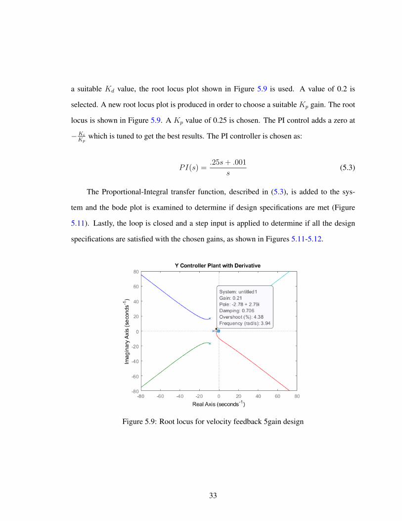
a suitable Kd value, the root locus plot shown in Figure 5.9 is used. A value of 0.2 is
selected. A new root locus plot is produced in order to choose a suitable Kp gain. The root
locus is shown in Figure 5.9. A Kp value of 0.25 is chosen. The PI control adds a zero at
−Ki
Kpwhich is tuned to get the best results. The PI controller is chosen as:
PI(s) =.25s+ .001
s(5.3)
The Proportional-Integral transfer function, described in (5.3), is added to the sys-
tem and the bode plot is examined to determine if design specifications are met (Figure
5.11). Lastly, the loop is closed and a step input is applied to determine if all the design
specifications are satisfied with the chosen gains, as shown in Figures 5.11-5.12.
Figure 5.9: Root locus for velocity feedback 5gain design
33

Figure 5.10: Root locus for proportional gain design
Figure 5.11: Y controller Bode plot
34

Figure 5.12: Step response of Y Controller
5.2 Linear-Quadratic-Regulator Design
In this section, and LQR controller is implemented for both inner and outer loops using
the previously mentioned double loop controller design. As with PID design, in order to
implement the LQR controllers the model must be linearized. Since that is already done,
the linear model can be utilized directly to implement the controllers. A full overview of
the LQR algorithm is covered in [20]. A brief description is given below to explain how
the design was completed. Consider the linear state space model:
x(t) = Ax(t) + Bu(t), t ≥ 0 (5.4)
where A ∈ Rn×n is the state matrix and B ∈ Rn×m in the input matrix. The state vector
x is of dimension n, and u is the input vector with m inputs. Clearly the pair (A,B) must
be controllable. Using the full state control law, u(t) = −Kx(t), the objective is to find
a suitable K ∈ Rn×m such that the close-loop system is asymptotically stable and that the
following cost function (5.5) is minimized [23].
35

J(K) =
∫ ∞0
[xT (t)Qx(t) + uT (t)Ru(t)
]dt (5.5)
Note that u here represents the input vector, not to be confused with motor commands
referenced in the dynamic model (2.9). Additionally, Q is positive definite matrix that
penalizes deviation from the system state equilibrium, while the positive definite matrix
R penalizes a large control input vector u for control efficiency. The feedback gain K is
determined by:
K = R−1BTP (5.6)
where P is a solution to Riccati’s Algebraic Equation:
PA + ATP + Q−PBR−1BTP = 0 (5.7)
The initial values of Q and R matrices can be chosen using the Bryson’s rule [15], but this
implementation uses values from previous research [20], and hand tuned for satisfactory
results. With A, B, Q, and R matrices defined, the values for K can be obtained using a
mathematical package, such as K = lqr(A,B,Q,R) in MATLAB.
5.2.1 Attitude Control Design
The LQR controller with integral action control structure is presented in Figure 5.13. This
is the same controller design used for roll, pitch, and yaw controls. The design finds the
feedback and integral gains for the three controllers simultaneously. Altitude control is
similar, however that design uses a different state space model, as seen in Section 5.2.2. To
obtain the appropriate K matrices for state feedback a new state space model is obtained.
36

Figure 5.13: LQR with integral diagram
Specifically, defined as:
γ = [φ θ ψ p q r]T
β = [τφ τθ τψ]T (5.8)
y = [φ θ ψ]T
where γ represents the new state variables β is the output vector, and y is the output. Thus,
the matrices in the state equation are:
Ae =
0 0 0 1 0 0
0 0 0 0 1 0
0 0 0 0 0 1
0 0 0 4.890 0 0
0 0 0 0 4.5366 0
0 0 0 0.1689 0.1149 −3.1622
(5.9)
Be =
0 0 0
0 0 0
0 0 0
100.0000 0 0
0 121.9512 0
0 0 67.5676
(5.10)
37

Hand tuned values for Q and R are
Qe = diag([.001 .001 2.01 .01 2 20 20 175]),R = diag([.05 .05 15]) (5.11)
As a result the gain matrix K and integral gains for attitude control are:
Ke =
4.6666 −0.0003 1.2843 0.5935 0.0005 0.2845
0.0007 4.6666 0.9329 0.0006 0.5635 0.2069
−0.0144 −0.0104 1.7558 0.0006 0.0004 0.3857
(5.12)
Ki =
[19.9944 19.9944 3.4102
](5.13)
5.2.2 Altitude Control Design
For altitude control, a simpler state space model is defined. Let
γ = [ze vz]T
β = U (5.14)
y = ze
where γ represents the new state variables, β is the input vector, and y is the output. There-
fore the linearized model is characterized by the following matrices:
Aalt =
0 1
0 −0.0206
,Balt =
0
0.8921
. (5.15)
38

The following Q, and R matrices are used
Qalt = diag([.5.510]), Ralt = diag([0.2]). (5.16)
As a result the feedback and integral gain are:
Kalt =
[6.2606 3.5886
],Kialt = 5.000 (5.17)
5.2.3 Outer Loop Design
For outer loop position control, the state space model is defined below. Let
γ = [xe ye vx vy]T
β = [φ θ]T (5.18)
y = [xe ye]T
where γ represents the new state variables, β is the input vector, and y is the output. The
state and input matrices are:
Axy =
0 0 1.0000 0
0 0 0 1.0000
0 0 −0.2060 0
0 0 0 −0.2060
(5.19)
Bxy =
0 0
0 0
0 9.8067
−9.8067 0
. (5.20)
39

Hand-tuned values for Q and R are
Qe = diag([.001 .001 2.01 .01 2 20 20 175]),R = diag([.05 .05 15]) (5.21)
The state feedback matrix Kxy and integral gains Kixy for position control are:
Kxy =
0.0000 0.3593 0.0000 0.2624
−0.3593 0.0000 −0.2624 0.0000
,Kixy =
[0.2191 0.2191
]. (5.22)
5.3 LQR Simulation Results
A combination of Simulink-based LQR model and MATLAB was used for simulation. The
diagram in Figure 5.14 shows the roll, pitch, and yaw inner loop controllers. Roll and pitch
results are presented in Figures 5.15 and 5.16. Design specifications from Chapter 5 are
met. The outer loop Simulink model is similar to that of Figure 5.14. As shown in Figures
5.17 and 5.18 the simulation response meets specifications.
Figure 5.14: LQR model for inner loop controllers
40

Figure 5.15: Roll controller step response
Figure 5.16: Pitch controller step response
41

Figure 5.17: X controller step response
42

Figure 5.18: Y controller step response
5.4 Backstepping with Adaptive Law Control Design
In this section, the fundamentals of backstepping design for attitude and altitude control is
presented. In addition, an adaptive control law presented in [3] is implemented for fault
tolerance in the event of a loss of effectiveness (LOE) fault in an actuator command output.
Backstepping follows a Lyapunov-stability based recursive design procedure [13]. First, a
nominal controller will be designed and implemented. Then, the adaptive control law will
be implemented to handle the actuator LOE.
In order to design the nominal control law, the quadrotor dynamic model (Chapter 2)
43

must be revisited. Specifically, the attitude and altitude dynamics are described by
ze = vz (5.23)
vz = g − 1
m(cdvz + cos(φ) cos(θ)U) (5.24)
η = Rη(φ, θ)ω (5.25)
ω =
Jy−JzJx
qr
Jz−JxJy
pr
Jx−JyJz
qp
+
1Jxτφ
1Jyτθ
1Jzτψ
+
1Jxξp
1Jyξq
1Jzξr
(5.26)
Following the backstepping design procedure given in [3], the state variables will be setup
as follows:
x1 , [ze, φ, θ, ψ]T (5.27)
x2 , [vz, p, q, r]T (5.28)
Using equations (2.8) and (5.23)-(5.26) the altitude and attitude dynamic equations
can be shown in a compact form:
x1 = g1(x1)x2 (5.29)
x2 = f2(x1, x2) + g2(x1)MΩ (5.30)
where Ω represents the motor command vector [u1 u2 u3 u4]T , M is the mapping matrix
44

given in (2.10) and
g1(x1) ,
1 0
0 Rn(φ, θ)
(5.31)
g2(x1) ,
− cos(φ) cos(θ)m
0
0 J−1
(5.32)
f2(x1, x2) ,
g − cdmvz
Jy−JzJx
qr
Jz−JxJy
pr
Jx−JyJx
pq
(5.33)
where J = diagJx, Jy, Jz
Let the desired reference vector be:
x1d , [vzd, φd, θd, ψd]T (5.34)
The following new variables are introduced:
z1 = c1(x1 − x1d) + c2
∫ t
0
(x1 − x1d)dτ (5.35)
z2 = q1 (5.36)
Since (x1 − x1d) can be considered an error signal, a gain c1 is introduced similar to a pro-
portional gain in conventional PID design. Likewise, an integral term is added to improve
steady state error, where c2 is the gain to the respective integral components. Both c1 and
c2 are positive diagonal matrices. Finally, a virtual control signal [3] is defined as:
q1 = (c1g1(x1))−1(c1 ˙x1d − z1 − c2(x1 − x1d) (5.37)
45

A Lyapunov function candidate is chosen:
V =1
2zT1 z1 +
1
2zT2 z2 (5.38)
Following the derivations show in [3] the following control signal is obtained
Ω = (g2(x1)M)−1(q1 − f2(x1, x2)− c1g1(x1)T z1 − c3z2) (5.39)
where c3 is another diagonal gain matrix. The motor command signals Ω can be sent
directly to the hardware.
5.4.1 Adaptive Law
If there is an actuator fault, a quadrotor could lose tracking ability as well as stability. An
adaptive law was derived in [3] to handle multiple actuator faults. The adaptive controller
will inherent many of the same aspects as the nominal controller, with some modifications
to the compact equations [3]:
x1 = g1(x1)x2 (5.40)
x2 = f2(x1, x2) + g2(x1)M
[(I4 −
4∑s=1
ϑsΛs
)Ω
](5.41)
where ϑs is an unknown fault parameter in one of the motors, s = 1, .., 4, and Λs is
composed of four diagonal fault distribution matrices, defined as Λ1 = diag(1, 0, 0, 0),
Λ2 = diag(0, 1, 0, 0), Λ3 = diag(0, 0, 1, 0), and Λ4 = diag(0, 0, 0, 1). A more thorough
derivation is given in [3]. where γs is the adaptive gain. Based on the Lyapunov stability
46

theory, the new control signal is [3]:
Ω =
g2(x1)M (I4 −
4∑s=1
(ϑsΛs
)−1 (q1 − f2(x1, x2)− c1g1(x1)T z1 − c3z2) (5.42)
and the adaptive law is
ϑs − γzT2 g2(x1)MΛsΩ (5.43)
where γ is an adaptive gain.
47

Experimental Results
In this chapter, some experimental results are shown to illustrate the effectiveness of the
controllers designed in Chapter 5.
6.1 PID Flight Test Results
6.1.1 Inner Loop
Multiple flights are executed to record flight data to show the tracking performance. For
the PID controller’s inner loop a specific flight is recorded where the quadrotor is moved
around the flight area in a square pattern. This allows for more variation in tracking than
a circular pattern. Figures 6.1 - 6.3 demonstrate the tracking performance results for roll,
pitch, and yaw angles. As can be seen, the tracking performance is satisfactory.
48

Figure 6.1: Tracking response for phi angle (PID controller)
Figure 6.2: Tracking response for theta angle (PID controller)
49

Figure 6.3: Tracking response for psi angle (PID controller)
6.1.2 Outer Loop
The outer loop performance tracking is presented in Figures 6.4 - 6.6. In this flight the
quadrotor is flown in a circular pattern for several minutes. A circular flight allows for
more discernible plot results. Throughout the flight thrust is applied to show tracking for
the Z position, shown in Figure 6.6. Again, the tracking performance is satisfactory.
Figure 6.4: Tracking response for X position (PID controller)
50

Figure 6.5: Tracking response for Y position (PID controller)
Figure 6.6: Tracking response for Z position (PID controller)
51

6.2 LQR Flight Test Results
6.2.1 Inner Loop
Similar to the PID inner loop tracking, the LQR inner loop flight is performed in a square
pattern over several minutes. The roll, pitch, and yaw angles are presented in Figures 6.7 -
6.9. As can be seen, actual angle tracks closely to the commanded angles.
Figure 6.7: Tracking response for phi angle (LQR controller)
52

Figure 6.8: Tracking response for theta angle (LQR controller)
Figure 6.9: Tracking response for psi angle (LQR controller)
6.2.2 Outer Loop
The outer loop performance tracking is presented in Figures 6.10 - 6.12. In this flight the
quadrotor is flown in a circular pattern for several minutes. Throughout the flight thrust is
applied to show tracking for the Z position, as shown in Figure 6.12. Clearly, the actual
position was able to closely track the commanded position.
53

Figure 6.10: Tracking response for X position (LQR controller)
Figure 6.11: Tracking response for Y position (LQR controller)
54

Figure 6.12: Tracking response for Z position (LQR controller)
6.3 Backstepping Flight Test Results
6.3.1 Nominal Case (Without Faults)
The backstepping controller results are presented here. This flight is also flown in a square
pattern allowing for some variation in the commanded angles. The PID outer loop con-
troller provides the commands for roll, pitch, and yaw angles to the backstepping inner
loop controller. The tracking performance is shown in Figures 6.13 - 6.16.
55

Figure 6.13: Tracking response for phi angle (backstepping controller)
Figure 6.14: Tracking response for theta angle (backstepping controller)
56

Figure 6.15: Tracking response for psi angle (backstepping controller)
Figure 6.16: Tracking response for Z position (backstepping controller)
57

6.3.2 Adaptive Backstepping Flight Test with Simulated Faults
In order to examine the adaptive controller’s functionality, faults must be inserted into the
control system. In this research, the faults are artificially injected into the motor commands
directly. To simulate the effect of actuator loss of effectiveness, which is compensated by
the adaptive law. The following experiments are considered: (1) a single fault is injected
into motor 1; (2) faults are injected to motor 1 and 2 sequentially, (3) faults are injected into
all four motors over the course of the flight. The flight performed is a fast, circular shape
executed several times. (While flying, there is a small ± 10 yaw as well as a small ± 5cm
altitude command applied to the vehicle).
6.3.2.1 Single Actuator Fault
A fault of 30% was injected at t = 20s directly into motor 1. After the fault occurs, the
attitude angles are quickly corrected and then are able to track the desired attitude angles
effectively. The X and Y positions experiences a brief deviation from the desired path but
also quickly recovers and is able to maintain satisfactory tracking performance. In Figure
6.19, it can be seen that adaptive law compensates for the 30% LOE by increasing the
motor command.
6.3.2.2 Double Actuator Faults
In this scenario two motor faults are implemented. The first motor fault follows the same
as the single fault case. It was injected with a 30% LOE at t = 20s. At t = 40s a secondary
LOE of 20% was injected into motor 4. After two faults occur simultaneously, for t ≥ 40s,
as shown in Figures 6.21 - 6.22 the adaptive controller was able to maintain satisfactory
tracking performance after a short transient. Figure 6.22 shows the compensated motor
commands.
58

Figure 6.17: Attitude tracking with 30% fault in motor 1 occurring at 20s
Figure 6.18: Position tracking with 30% fault in motor 1 occurring at 20s
59
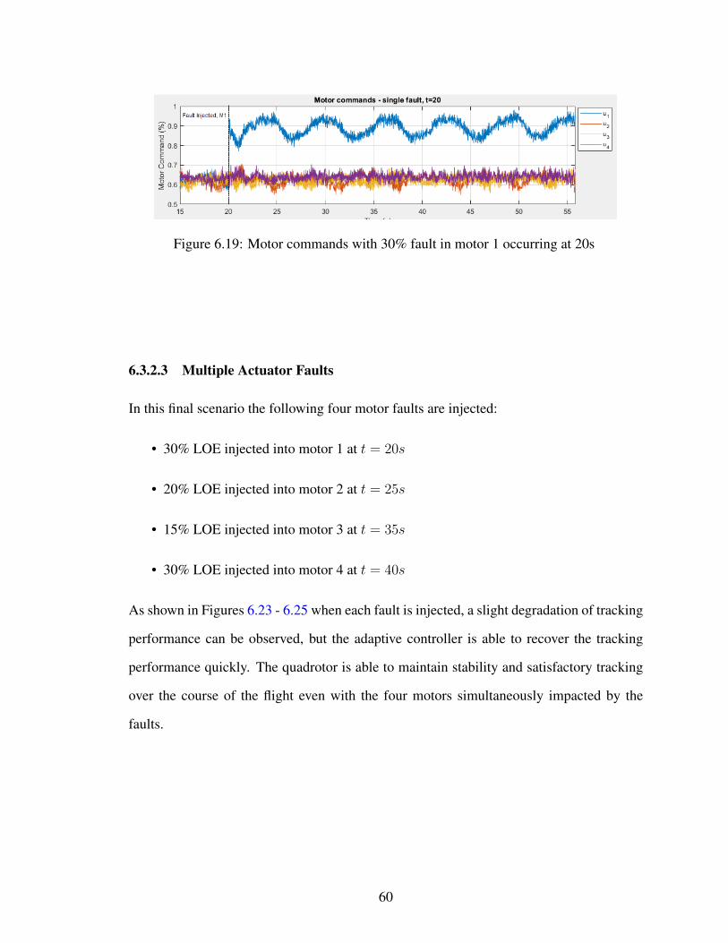
Figure 6.19: Motor commands with 30% fault in motor 1 occurring at 20s
6.3.2.3 Multiple Actuator Faults
In this final scenario the following four motor faults are injected:
• 30% LOE injected into motor 1 at t = 20s
• 20% LOE injected into motor 2 at t = 25s
• 15% LOE injected into motor 3 at t = 35s
• 30% LOE injected into motor 4 at t = 40s
As shown in Figures 6.23 - 6.25 when each fault is injected, a slight degradation of tracking
performance can be observed, but the adaptive controller is able to recover the tracking
performance quickly. The quadrotor is able to maintain stability and satisfactory tracking
over the course of the flight even with the four motors simultaneously impacted by the
faults.
60

Figure 6.20: Attitude tracking with 30% fault in motor 1 occurring at 20s, and 20% fault inmotor 4 at 40s
Figure 6.21: Position tracking with 30% fault in motor 1 occurring at 20s, and 20% fault inmotor 4 at 40s
61

Figure 6.22: Motor commands with 30% fault in motor 1 occurring at 20s, and 20% faultin motor 4 at 40s
Figure 6.23: Attitude tracking with multiple faults occurring
62

Figure 6.24: Position tracking with multiple faults occurring
Figure 6.25: Motor commands multiple faults occurring
63

Hardware and Software II
7.1 Quadrotor Hardware
A laser rangefinder, is introduced and mounted on the top of the quadrotor as shown in
Figure (7.1). The height of the laser could potentially block the cameras on the Vicon
positioning system, so a marker is mounted on top to create an additional point for object
creation. A small USB hub (not visible) is also mounted for the laser and joystick remote
for direct access.
The laser rangefinder is a Hokuyo model URG-04LX-UG01 which is capable of mea-
suring about 720 distinct points around a 240 field of view. The rangefinder can detect
objects between 20mm-5600mm.
7.2 Ubuntu and Docker
As stated in Chapter 3, the quadrotor is running an embedded Linux Yocto system. It is
difficult to add software to the quadrotor without serious risk to the OS integrity. Fortu-
nately, the OS has a docker daemon running that can be used after some initial setup and
network configuration. Docker is a software package that allows the creation of a sand-
boxed container to allow for research and development without affecting the host system.
The kernel between the host OS and docker OS is the same, so any kernel modifications
64

Figure 7.1: Quadrotor with mounted laser rangefinder
must be done on the host OS. However, the OS deployed into the container can be almost
any. This research is utilizing Ubuntu Xenial in the docker container for compatibility and
ease of installation of ROS (Robot Operating System). Docker has built in network capa-
bilities that will allow external applications to have direct access to its resources. With both
Docker and ROS implemented in the system, the new architecture is in Figure 7.2.
Figure 7.2: System architecture
65

7.3 Robot Operating System
ROS has become a popular tool for hobbyists and professionals to implement a vast array
of software and capabilities on embedded systems. ROS itself is not an operating system,
but allows for interprocess communications to occur between nodes [11]. The architecture
of ROS (Figure 7.3) consists of several components. ROS Master (roscore) is the central
piece of management in the topology. It handles managing names and registration services
for the nodes as well as facilitating inter-node communications. A node is a specific ROS
API integrated program that can publish, subscribe to topics, and communicate with other
nodes. Nodes can be written in an assortment of languages, like C, C++, and Python. A
publisher (which can be a node) transmits a message to the ROS system. That message
is retained, and subscribers are able to pick it up. A topic is a ROS specific data defini-
tion. There are hundreds of topics developed, and custom topics can be implemented if
necessary. This implementation uses all of these platform components.
In this research, ROS is implemented with a SLAM node that allows for mapping
capabilities. Finally, path planning, obstacle navigation and avoidance are described in
Chapter 8.
Figure 7.3: ROS system model
66

7.3.1 LIDAR Driver
A laser rangefinger driver is implemented as a ROS node. The node communicates to
the USB-attached hardware and publishes the raw scanned data in a ROS topic called scan.
The scanned data consists of 720 floating point values representing the distance of potential
obstacles from that specific point on the laser.
7.3.2 Laser Scanner Matcher
Another node that functions as both a publisher and subscriber. This node subscribes to
the scan laser topic and is capable of performing fast and accurate odometry. The results
are published in the pose2D topic. The published topic consists of an estimate of the 2D
position as well as the yaw angle. The laser scan matcher provides the pose estimate at
15Hz, which is fast enough to be used as the quadrotors current position without modifi-
cation. The mapping and path planning algorithm will use this pose information instead
of Vicon’s estimate. Even though the laser scanner is fast and robust, it has limitations.
The pose is generated from the laser’s 720 depth readings, and it is possible to confuse the
laser scan matcher if sufficient depth information is not available. This can happen in a
long hallway or large rooms that do not have many features available. The scanner uses
IMU data published on the imu topic to increase its accuracy. The quadrotor’s flight control
system provides IMU data through a ROS node.
7.3.3 Pose2D Server
The pose2d server was written from scratch to facilitate obtaining the odometry from the
pose2d topic and providing it to the quadrotor for its position. Likewise, this software
receives six data points from the quadrotor’s IMU and publishes this to the imu topic for
use by the laser scanner. In addition, this software integrates with rviz (ROS Visualization)
by publishing an image (called markers) of the quadrotor to be viewed in the visualization
67

package, as shown in Figure 7.4
Figure 7.4: Drone visualized by ROS
7.3.4 Gmapping
The last item needed to build upon is called Gmapping. Gmapping subscribes to the pub-
lished laser data and generates an occupancy map which is published to the map topic. This
map is simple, in that there are three states: an obstacle, free space, and unknown space.
Unknown space is determined as being out of range of the laser or behind an obstacle. Free
space is determined as an area without a known obstacle and is not unknown space. An
example occupancy map is visualized in Figure 7.5
7.3.5 ROS Visualization
ROS Visualization, is a powerful GUI that can be used for inspection of ROS internals. This
includes maps, pose data, or other visual. This research implements many visualizations
during the development for troubleshooting and for proof of functionality. Rviz can be used
interactively during program execution for a real-time dashboard into the ROS platform.
68

Figure 7.5: GMapping occupancy map
69

7.4 Platform Architecture
Figure 7.2 represents the system platform with ROS. All devices are connected to a central
access point to reduce latency. Routing is configured to allow network access in and out
of the docker container running inside the quadrotor. The controller connects to an RF
dongle that is plugged directly into the quadrotor. Custom software is implemented that
runs in the container with direct hardware access to the USB dongle. This is required
since the quadrotor’s host operating system does not have the capabilities to execute this
code. Position, previously acquired from Vicon, is now provided through the ROS pose2D
topic and send to the flight controller. While the software is still executed natively on the
quadrotor’s CPU, it is containerized and therefore isolated. The integration between the
docker container and the host OS is done using TCP/IP networking.
Figure 7.6 describes the ROS architecture specifically. As mentioned above, the laser
driver connects to the USB laser directly and publishes the raw scan data in the scan topic.
The laser scanner subscribes to the both the scan and imu topics while publishing pose
information in two formats. The quadrotor connects to the Pose2D server via TCP/IP and
sends IMU data while receiving the pose data. The Pose2D server publishes the IMU data
to imu and subscribes to the pose2d topic containing the pose information. Additionally,
the Pose2D server publishes the drone topic which is a visual representation of the drone,
respecting the yaw angle. The gmapping node subscribes to the both the scan data and pose
information. The SLAM algorithm processes the scan and pose data and then publishes an
occupancy grid to the map topic. The path planning software subscribes to the pose2d
topic to retrieve the quadrotor’s current position within the map. It also subscribes to the
scan topic in order to use the laser scanner directly for obstacle detection, as discussed
in chapter 8. The map topic is also subscribed to obtain the latest SLAM map. The map
is modified internally to include bounding boxes which is used as buffer space for the
quadrotor, which is discussed in Section 8.1. The modified map is published back to the
ROS topic scaled map along with mutiple topics that are generated on the fly and published
70

for visual effects.
Using rviz, the topics can be connected and the visuals on the right of Figure 7.6 can
be achieved. These visual enhance the development process, debugging, and also provide
a method to present platform effectively.
Figure 7.6: ROS architecture
71

Mapping and Path Planning
Path planning is an important mechanism for autonomous robots to find the shortest or op-
timal path between two points. There are many algorithms designed to find paths between
two points. In this research two algorithms were implemented with modest changes to them
based on [8].
One challenge with path planning while using a mapping algorithm, like SLAM, is
that the map has undiscovered regions. Path planning is best applied when a map is already
known [12]. The algorithm must consider these regions as open space in order to build
an initial path. As the map is discovered via flight, previously undiscovered regions may
appear as obstacles. These newly determined obstacles may conflict with the previously
determined path. When this occurs, a new path must be generated from the quadrotor’s
current location to the goal.
8.1 Map Preparation
In order to plan a path, an occupancy map (Figure 7.5) must be converted internally to a
map that the respective algorithm can understand. Not only must the map be converted,
but also any obstacles need to have an extra buffered layer presented as an obstacle around
it. Because the laser ranger is located in the center of the quadrotor, there is approximately
20cm from the center of the quadrotor to the perimeter of the quadrotor. Path planning
algorithms are not aware of the quadrotor’s physical properties and only of the environ-
72

ment. By adding obstacle buffered space to the map, the obstacles will compensate for the
quadrotor’s physical properties.
Once an occupancy map is obtained from the map topic, it is immediately processed.
A new map is generated and presented to the path planning subsystem. Figure 8.1 shows
the original map and the obstacle map side-by-side. Additionally, having this secondary
map that can be modified is very useful for other applications, as described in Section 8.4.
Figure 8.1: Left: occupancy map. Right: obstacle boundary map.
8.2 A* Path Planning
A* takes a heuristic approach to path planning, by looking at adjacent nodes [14]. A
node, for this implementation, is considered one map block. The size is dependent on
the map resolution. In this research A* was discovered to find a path quickly. However,
the A* algorithm will build a path very close to obstacles, so a buffer space is required.
Additionally, one path is created per node, which creates many smaller individual steps.
73

This can be adjusted in the algorithm by extending the neighbor search, but must be done
with care. Otherwise the path will cut corners through obstacles. Figure 8.2 is an example
Figure 8.2: A* mapping example
of the visualizations that were built next to the physical flying space. On the left is the
occupancy map, with the bounding map overlaid. The quadrotor is depicted (from the
pose2d server described in Section 7.3.3), along with the path points from the algorithm.
Lastly, the green dot represents the goal. The goal point is in the unknown map space. As
the quadrotor flies, and the map becomes revealed, if there is an obstacle there, the path is
regenerated. The right side shows the working environment, in a low resolution photo. It
can be seen how the physical obstacles correspond to the map, and the tight spaces between
them.
8.3 Rapidly Exploring Random Tree* Path Planning
RRT is another method to path planning, but is not guaranteed to find the optimal path.
It is based on random sampling of configuration space [24] (the map). The samples are
connected in a tree-like structure, and a path is generated from those trees. RRT* expands
on RRT by adding a neighbor search and rewiring operation covered here [8]. RRT* has a
built in obstacle detection mechanism that can be configured, and it is not always optimal.
74

For instance, a path may be generated that traverses known obstacles as shown in Figure
8.3. If the environment is too complex, RRT* is unable to generate a path. There are
Figure 8.3: RRT* going through obstacles
two visuals added in Figure 8.3. Yellow dots represent ”soft obstacles”, which are on the
bounding box mentioned in Section 8.1. Red dots are the known map obstacle. Both are
treated as obstacles, but distinguished. As with A*, if there is an obstacle revealed during
map discovery, a new path is generated. This can be seen in Figures 8.4, and 8.5. In Figure
8.4, a path is generated and traversed. As the SLAM algorithms reveals more of the known
map, it is seen in Figure 8.5 that the existing path passed through a ”soft obstacle”. A new
path is generated after a few tries, as shown in Figure 8.6. The red square in Figure (8.4)
indicates where an obstacle will be detected. The edge of the bounding box is detected in
flight, as shown in Figure 8.5.
75

Figure 8.4: RRT* generated path
Figure 8.5: RRT* newly generated path
Figure 8.6: Final path generated by RRT*
76

8.4 Dynamic Obstacle Avoidance
In this research it is also explored if the quadrotor can effectively detect and avoid dynamic
obstacles. The major challenge with this concept is the mapping system. An occupancy
map handles transitions quickly. A transition from an unknown space to an obstacle can
be almost immediate. However, a transition from an open space to an obstacle is not core
functionality as the map is intended to be static. Introducing a random obstacle into a
previously known open space may cause a crash with the obstacle that is not timely detected
by the quadrotor.
The laser rangefinder’s scan data is already published and being used in by the quadro-
tor. With a scanning algorithm designed, the front of the quadrotor can be monitored for
quickly changing depths, and react accordingly. A brief overview of the algorithm is as
follows:
• A selected range from the scan data is chosen and monitored. The distance monitored
is within 2m of the quadrotor.
• Each scanned obstacle’s velocity is calculated by using the prior scan and time be-
tween scans. The obstacles are stationary, but the quadrotor is not. The velocity
calculated is the quadrotor’s velocity with respect to the specific scanned location.
Velocity values that are greater than 10m/s warrant additional investigation.
• Examine the map data where the scanned value’s velocity has exceeded 10 m/s. If
the map data represents a known obstacle, it is ignored.
• If the map data is unknown or empty space, the obstacle that has been detected is
assume to be dynamically placed.
• The quadrotor stops navigation and plans a new route with the knowledge of the new
obstacle.
77

Since the laser rangefinder has a 240 range, using a portion of this data in the front
will allow the programs to detect unexpected obstacle. Over multiple laser scans the ve-
locity of each scanned data point is calculated using the change in depth data with respect
to the scan rate (15Hz). If the velocity, within a 2m range, exceeds 10m/s (set experimen-
tally) then that is enough to warrant additional logic. If the quadrotor is flying towards an
obstacle it needs to be determined if that is already known or in unknown/free space. If
this condition is met, the map is checked in the area where the detection occurred. If the
occupancy map has a known obstacle, it is ignored. However, if the map does not represent
an obstacle where the laser detected something, it is considered unexpected. Since a new
map is generated from the original occupancy grid (Figure 8.1), the bounding map is ex-
plicitly modified to include the unexpected obstacle. This will allow for the path planning
algorithms to renegotiate the path.
Figures (8.7) - (8.9) demonstrate a successful implementation of this method.
Figure 8.7: Target path generated
78

Figure 8.8: Obstacle appears in path
Figure 8.9: New path is generated
79

Conclusions and Future Research
9.1 Summary of Flight Control Algorithms
One of the goals of this research was to implement multiple quadrotor control laws, given
certain pre-determined specifications, and then conduct flight tests to verify the effective-
ness of the control algorithms.
First, an identification of the system model was required. Using the collected flight
data, a reasonably accurate quadrotor model was obtained using the least squares method.
With a quadrotor model, linearization is then conducted to obtain a linearized model re-
quired for control law design.
The first design was using a PID controller with velocity feedback. Gains were de-
termine using the root locus method. The specifications were verified during the design
phase with bode plots and step response plots. Inner loop and outer loop control laws
were designed. Then the PID laws were implemented on the quadrotor to demonstrate the
effectiveness of the control algorithm using real-time flight tests.
Next, an LQR design was conducted. Gains were determined by selected weighing
matrices Q and R. Specifications were confirmed using MATLAB simulation based on the
quadrotor’s dynamic model. Finally, the LQR laws were implemented and deployed to the
onboard hardware. Both inner and outer loop flight results were presented.
The last portion of the design phase consists of an adaptive backstepping algorithm.
A nominal flight controller was first implemented. Then, using an adaptive control law, the
80

ability to handle a loss of actuator effectiveness is implemented. The adaptive controller
was able to automatically compensate for the loss of effectiveness by modifying the motor
command. Satisfactory results of the adaptive laws were demonstrated using real time flight
tests.
Prior research has covered these topics on varying hardware platforms. This re-
search implement and validates the PID, LQR, and backstepping control algorithms for
the QDrone platform.
9.2 Summary of Mapping Results
SLAM was implemented with position information being provided to the quadrotor’s flight
controller for real-time flight control. With this information the quadrotor can navigate
without the constraints of the Vicon positioning system. Software was developed to inte-
grate the quadrotor’s IMU data combined with the laser scan data’s estimated pose for use
in the flight controller and to build a visualization platform. Building on top of a stable
mapping platform, two path planning algorithms are explored, including A* and RRT*.
Software was developed to navigate the drone through a set of paths provided by the al-
gorithms, while presenting the data to the visualization backend. One of the objectives of
this research is to implement a robust path planning system based on a map that is not fully
known and continually changing. Finally, it is desirable to be able to quickly detect and
react to an unexpected obstacle in the environment. This was successfully implemented
and demonstrated by implementing ROS and integrating SLAM with custom software and
nodes.
81

9.3 Future Research
The research area of indoor SLAM is fascinating, and there are multiple avenues that can
be used to enhance the result of this research. Firstly, the A* algorithm creates many small
path points between nodes. Because the quadrotor must ”ramp up” and ”ramp down” from
each point, the appearance of continuous flight when using A* is not ideal. A different
algorithm could be implemented, but custom manipulations of the generated path, while
avoiding obstacles could be implemented.
While Gmapping is a well-known SLAM implementation that uses Rao-Blackwellized
particle filtering [9], there are other interesting SLAM implementations that could be ex-
plored, including Visual SLAM and graph-based SLAM. In this research, ROS, SLAM
control software are all implemented directly on board the quadrotor. However, there is an
underlying need for a network due to the control software deployment using Simulink.
Therefore, it could also be possible to offload some of the computation of these cpu-
expensive SLAM algorithms to a high-end laptop.
The laser scan matcher can possibly fail due to lack of features. This causes the posi-
tion estimate to become stale, which creates a problem for SLAM and the flight controller
algorithms. The quadrotor has a downward facing camera which could be used for opti-
cal flow. Additionally, with a front facing camera capable of RGB, IR and depth readings
and it would be interesting to enhance the SLAM capabilities by adding a visual SLAM
component.
82

Bibliography
[1] Szabo P. Andrew. System identification and model-based control of quadcopter uavs.
Master’s thesis, Wright State University, 2019.
[2] D. Atherton, Kelsey. Can the army secure an american-made quadcopter? 2019.
[3] Remus C. Avram. Fault Diagnosis and Fault-Tolerant Control of Quadrotor UAVs.
PhD thesis, Wright State University, 2016.
[4] Roland Beard and Timothy McLain. Small Unmanned Aircraft: Theory and Practice.
New Jersey, 2012.
[5] S. Bouabdalla, P. Murrieri, and R. Siegwart. Design and control of an indoor micro
quadrotor. International Conference on Robotics and Automation, 2004.
[6] Roland Buchi. Fascination Quadrocopter. South Carolina, 2011.
[7] Petros Ioannou Baris Fidan. Adaptive Control Tutorial. South Carolina, 2006.
[8] Maximillion A. Gilson. Fault-tolerant mapping and localization for quadrotor uav.
Master’s thesis, Wright State University, 2019.
[9] Giorgio Grisettia, Gian Diego Tipaldi, Cyrill Stachniss, Wolfram Burgard, and
Daniele Nardi. Fast and accurate slam with rao–blackwellized particle filters.
Robotics and Autonomous Systems, 2007.
83

[10] G.M. Hoffmann, D.G. Rajnarayan, S.L. Waslander, D. Dostal, J.S. Jang, and C.J.
Tomlin. The stanford testbed of autonomous rotorcraft for multi agent control (star-
mac). In the Proceedings of the 23rd Digital Avionics System Conference, page 12,
2004.
[11] Lentin Joseph. PID Controllers: Theory, Design, and Tuning. 2017.
[12] Gregor Klancar, Andrej Zdesar, and Igor Skrjanc. Wheeled Mobile Robotics. 2017.
[13] Miroslav Krstic. Nonlinear and Adaptive Control Design. 2010.
[14] Akshay Kumar, Guruji Himansh, and Agarwal D.K.Parsediya. Time-efficient A* Al-
gorithm for Robot Path Planning. 2016.
[15] Emmanuel Okyere, Amar Bousbaine, Gwangtim T. Poyi, Ajay K. Joseph, and Jose M.
Andrade1. Lqr controller design for quad-rotor helicopters. The Journal of Engineer-
ing, 2018.
[16] Kevin Passino. Biomimicry for Optimization, Control,and Automation. New York,
2005.
[17] Quanser. Drone parameterization. 2018.
[18] Quanser. Embedded compute module. 2018.
[19] Quanser. Propulsion system. 2018.
[20] Muneeb Masood Raja. Extended kalman filter and lqr controller design for quadrotor
uavs. Master’s thesis, Wright State University, 2017.
[21] Zhang Sheng and Qian Wei-qi . Dynamic backstepping control for pure-feedback
nonlinear systems. The Journal of Engineering, 2017.
[22] Karl Johan Astrom and Tore Hagglund. PID Controllers: Theory, Design, and Tun-
ing. New York, 1995.
84

[23] Jovitha Jerome Vinodh Kumar E. Robust lqr controller design for stabilizing and
trajectory tracking of inverted pendulum. ScienceDirect, 2013.
[24] Vojtech Vonasek, Jan Faigl, Tomas Krajnık, and Libor Preucil. RRT-path – A Guided
Rapidly Exploring Random Tree. 2009.
[25] the free encyclopedia Wikipedia. Pid controller. 2020.
[26] Warren R. Young. The Helicopters. Time Life Books, Chicago, 1982.
85