quadtree displacement mapping with height blending practical detailed multi-layer surface rendering...
TRANSCRIPT

Quadtree Displacement Mappingwith Height Blending
Practical Detailed Multi-Layer Surface Rendering
Michal DrobotTechnical Art Director
Reality Pump
Outline
• Introduction• Motivation• Existing Solutions• Quad tree Displacement Mapping• Shadowing• Surface Blending• Conclusion

Introduction
• Next generation rendering– Higher quality per-pixel
• More effects• Accurate computation
– Less triangles, more sophistication• Ray tracing• Volumetric effects• Post processing
– Real world details• Shadows• Lighting• Geometric properties

Surface rendering
• Surface rendering stuck at– Blinn/Phong
• Simple lighting model
– Normal mapping• Accounts for light interaction modeling• Doesn’t exhibit geometric surface depth
– Industry proven standard• Fast, cheap, but we want more…
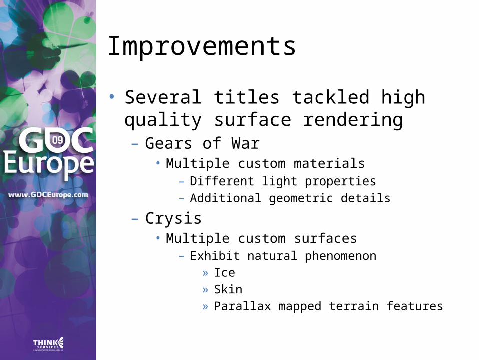
Improvements
• Several titles tackled high quality surface rendering– Gears of War
• Multiple custom materials– Different light properties– Additional geometric details
– Crysis• Multiple custom surfaces
– Exhibit natural phenomenon» Ice» Skin» Parallax mapped terrain features

Terrain surface rendring
• Rendering terrain surface is costly– Requires blending
• With current techniques prohibitive
– Blend surface exhibit high geometric complexity

Surface properties
• Surface geometric properties– Volume– Depth– Various frequency details
• Together they model visual clues– Depth parallax– Self shadowing– Light Reactivity

Surface Rendering
• Light interactions– Depends on surface microstructere– Many analityc solutions exists
• Cook Torrance BRDF
• Modelling geometric complexity– Triangle approach
• Costly– Vertex transform– Memory
• More usefull with Tessalation (DX 10.1/11)
– Ray tracing
Motivation
• Render different surfaces– Terrains– Objects– Dynamic Objects
• Fluid/Gas simulation
• Do it fast– Current Hardware– Consoles (X360)– Scalable for upcoming GPUs
• Minimize memory usage– Preferably not more than standard normal
mapping– Consoles are limited

Motivation
• Our solution should support– Accurate depth at all angles– Self shadowing– Ambient Occlusion– Fast and accurate blending


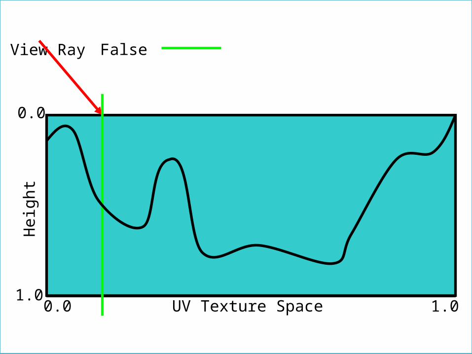
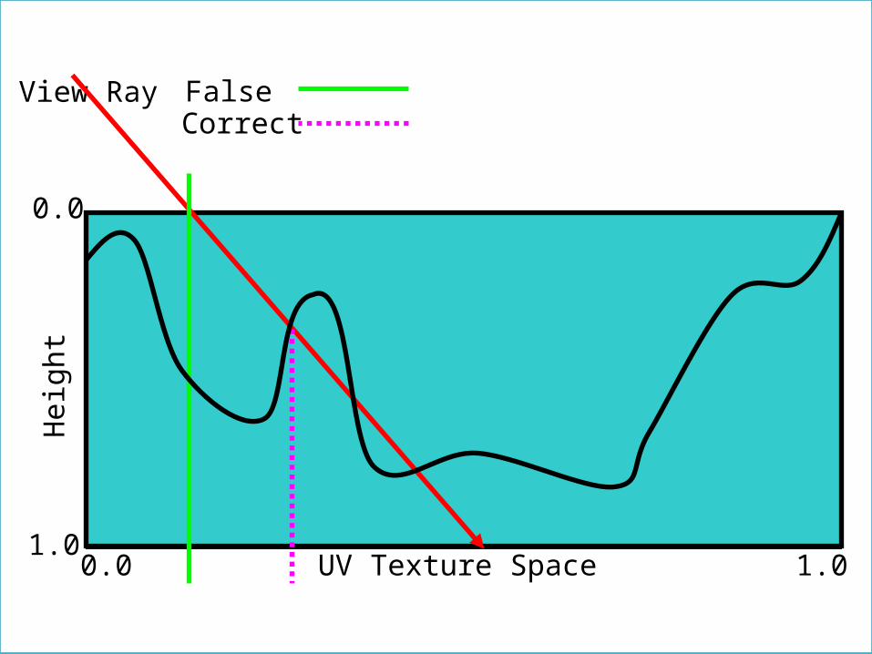
Existing Solutions
• Depth complexity– Calculate correct surface depth
• Find correct view ray – height field intersection
– Compute lighting calculation using calculated depth offset
View Ray FalseH
eig
ht
0.0
0.01.0
1.0UV Texture Space
View Ray FalseH
eig
ht
0.0
0.01.0
1.0UV Texture Space
Correct

Online methods
• Perform ray tracing using height field data only
• Additional memory footprint– 1x8 bit texture– May use alpha channel– DXT5 – OK!
• Remember about alpha interpolation!
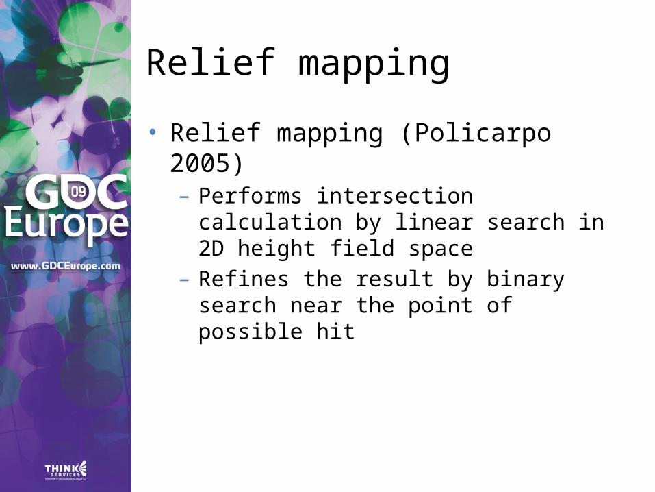
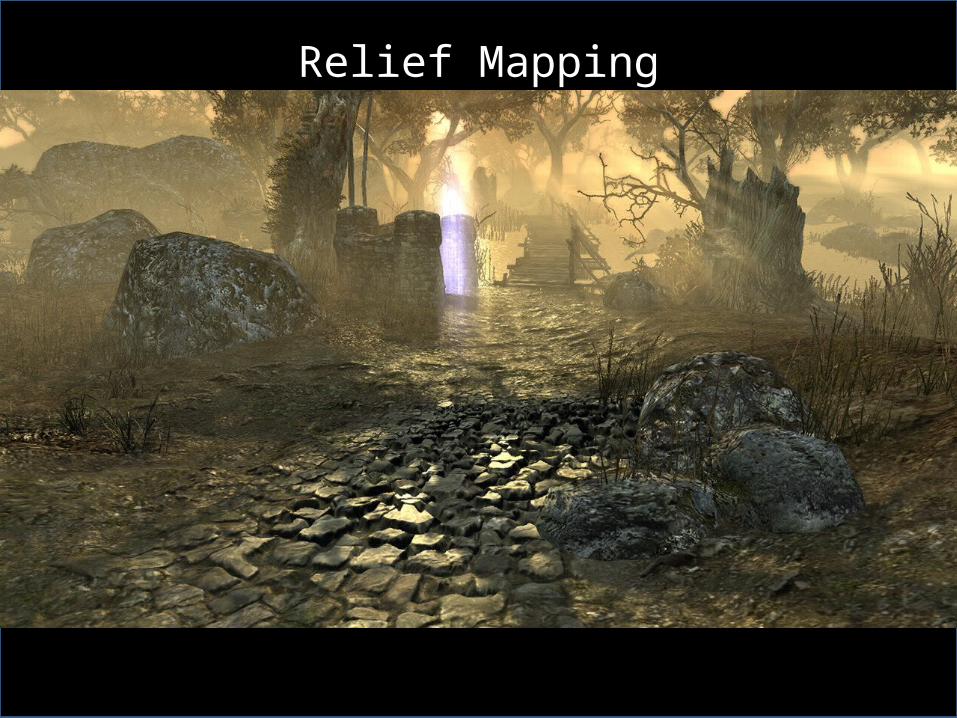
Relief mapping
• Relief mapping (Policarpo 2005)– Performs intersection calculation by
linear search in 2D height field space– Refines the result by binary search
near the point of possible hit
View Ray FalseH
eig
ht
0.0
0.01.0
1.0UV Texture Space
Correct
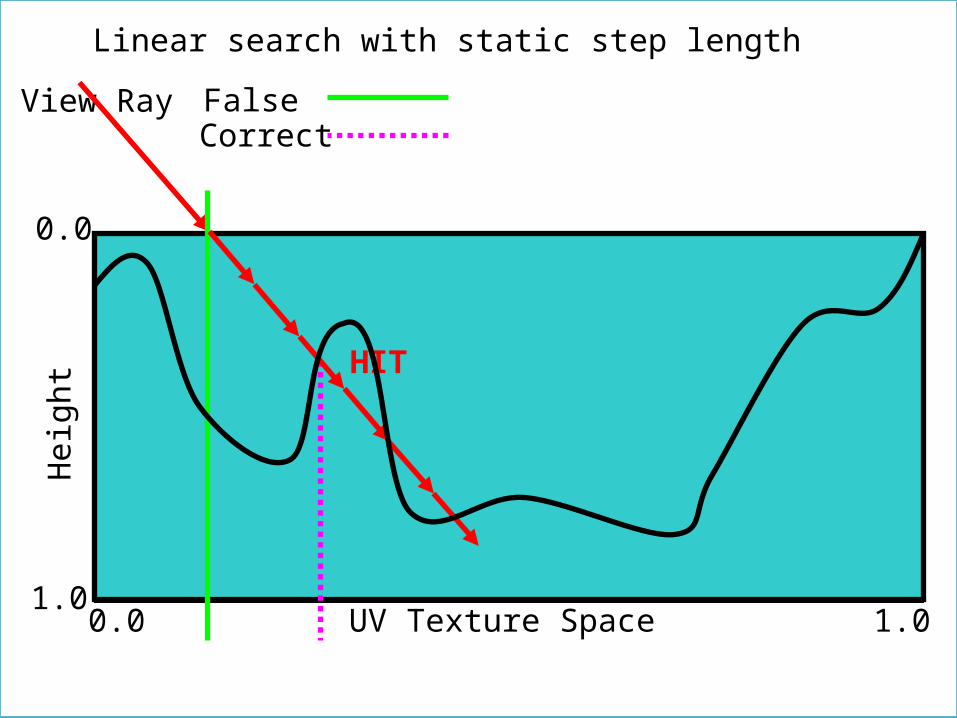
Linear search with static step length
HIT

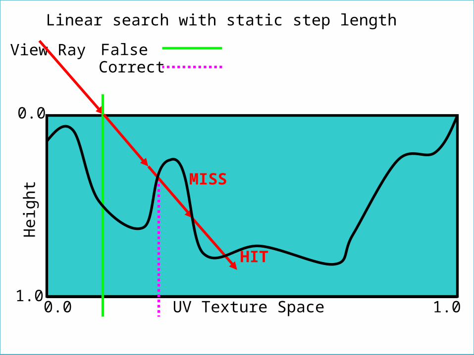
Linear Search
• Linear search in each step– Check if ray over height field– If YES
• Move the ray by const distance
– If NOT• Stop and go to Binary Search
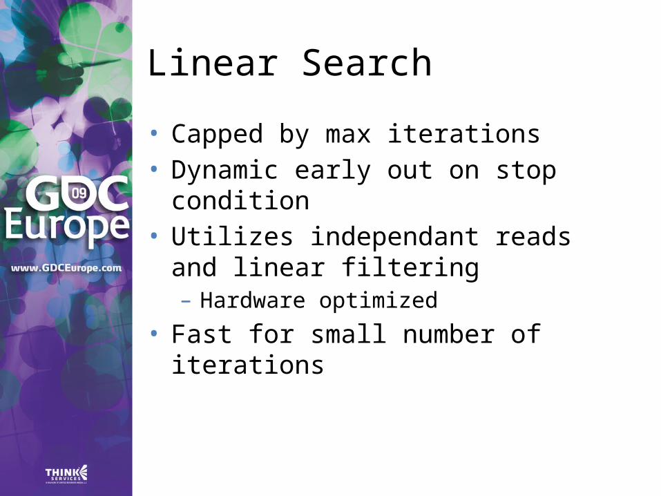
Linear Search
• Capped by max iterations• Dynamic early out on stop
condition• Utilizes independant reads and
linear filtering– Hardware optimized
• Fast for small number of iterations
Linear Search
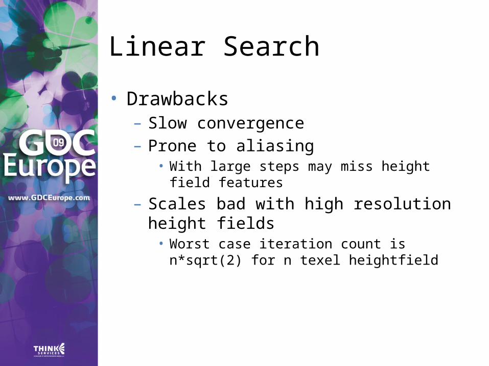
• Drawbacks– Slow convergence– Prone to aliasing
• With large steps may miss height field features
– Scales bad with high resolution height fields• Worst case iteration count is n*sqrt(2) for
n texel heightfield
View Ray FalseH
eig
ht
0.0
0.01.0
1.0UV Texture Space
Correct
Linear search with static step length
HIT
MISS

Binary Search
• Static number of iterations• Performs search along last step
vector• Converges fast• Utilizes linear filtering
Binary Search
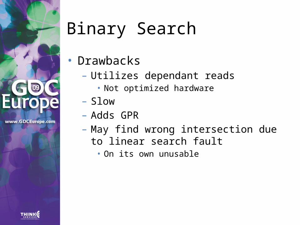
• Drawbacks– Utilizes dependant reads
• Not optimized hardware
– Slow– Adds GPR– May find wrong intersection due to
linear search fault• On its own unusable

View Ray FalseH
eig
ht
0.0
0.01.0
1.0UV Texture Space
Correct
Binary search with static step length
Binary search region

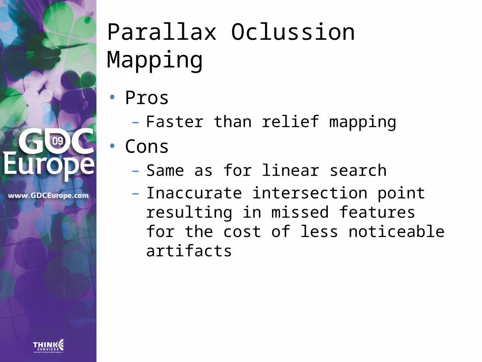
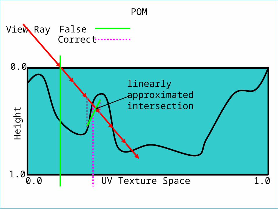
Parallax Oclussion Mapping
• POM (Tatarchuk 06)– Substitiutes costly binary search by
piecewise linear approximation using ALU
– Adds several performance improvements to linear search• Dynamic iteration count• LOD system• Approximate soft shadows
Parallax Oclussion Mapping
• Pros– Faster than relief mapping
• Cons– Same as for linear search– Inaccurate intersection point resulting
in missed features for the cost of less noticeable artifacts
View Ray FalseH
eig
ht
0.0
0.01.0
1.0UV Texture Space
Correct
POM
linearlyapproximatedintersection
Preprocessed method
• Several methods rely on preprocessed data– Per-pixel Displacement with Distance
Function• Using additional 3D textures rising
memory footprint to much• Impractical
– Cone Step Mapping– Relaxed Cone Step Mapping

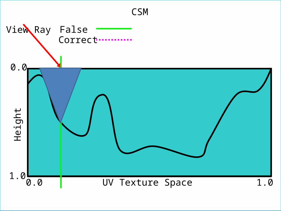
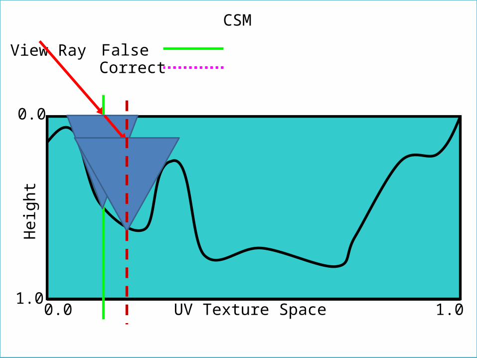
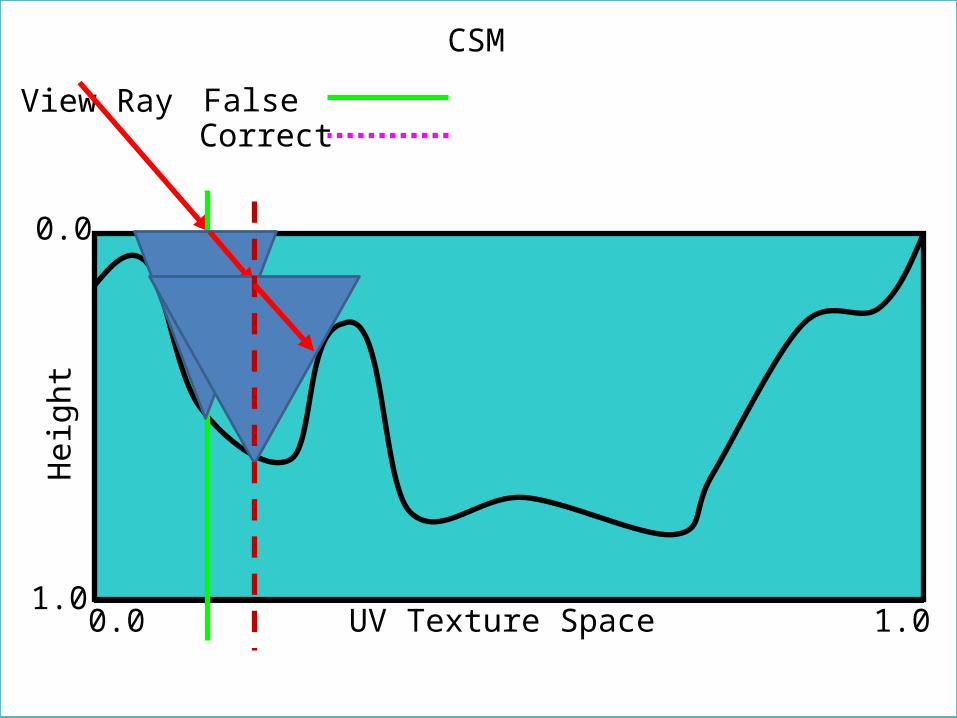
Cone Step Mapping
• CSM (Dummer 2006)– Based on Cone Maps
• Associate circular cone to each texel of height field
• Per-texel cone is the largest cone, not intersecting the height field
– Performs linear search with step length determined by actual cone radius• Leaps empty space
– Conservative approach• Allows accurate intersection computation
– Requires additional uncompressed 1x8bit texture for cone angles

Cone Step Mapping
• Pros– Very fast
• Requires significantly smaller number of iterations than pure linear methods
• Under-sampling provides distortions artifact, less noticeable than interleaving
– Accurate• There is no possibility to miss a feature
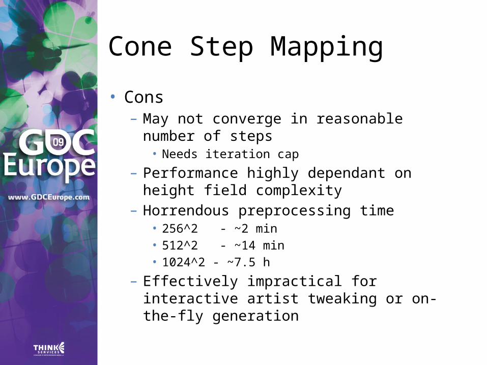
Cone Step Mapping
• Cons– May not converge in reasonable
number of steps• Needs iteration cap
– Performance highly dependant on height field complexity
– Horrendous preprocessing time• 256^2 - ~2 min• 512^2 - ~14 min• 1024^2 - ~7.5 h
– Effectively impractical for interactive artist tweaking or on-the-fly generation
View Ray FalseH
eig
ht
0.0
0.01.0
1.0UV Texture Space
Correct
CSM

View Ray FalseH
eig
ht
0.0
0.01.0
1.0UV Texture Space
Correct
CSM
View Ray FalseH
eig
ht
0.0
0.01.0
1.0UV Texture Space
Correct
CSM
View Ray FalseH
eig
ht
0.0
0.01.0
1.0UV Texture Space
Correct
CSM

View Ray FalseH
eig
ht
0.0
0.01.0
1.0UV Texture Space
Correct
CSM
HIT
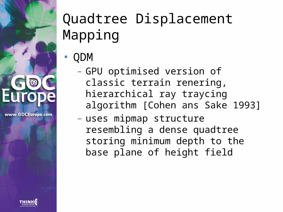
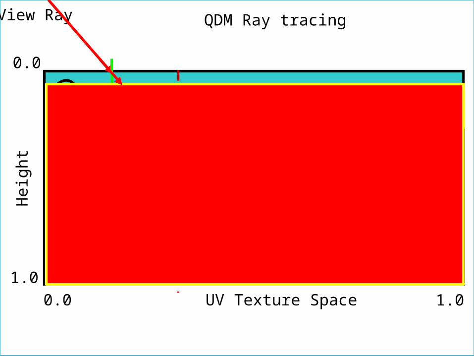
Quadtree Displacement Mapping• QDM– GPU optimised version of classic
terrain renering, hierarchical ray traycing algorithm [Cohen ans Sake 1993]
– uses mipmap structure resembling a dense quadtree storing minimum depth to the base plane of height field

Quadtree Structure
• Simple construction– Mipmapping with min operator
instead of average
• Hardware optimized• Small memory footprint– 1x8bit texture with MipMaps

Quadtree Structure
• Quadtree can be generated on-the-fly– Neglible performance loss
GF 8800 256^2 512^2 1024^2 2048^2
Quadtree 0.15ms 0.25ms 1.15ms 2.09ms
CSM < 2min <14 min <8h /
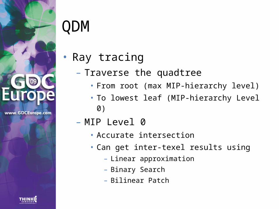
QDM
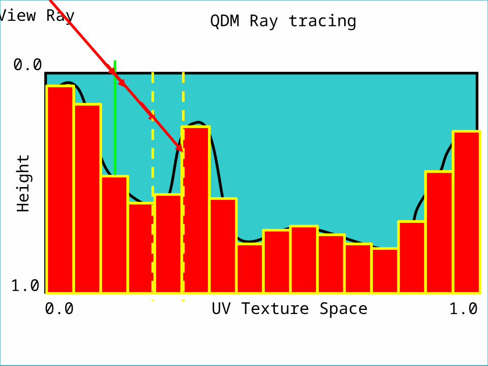
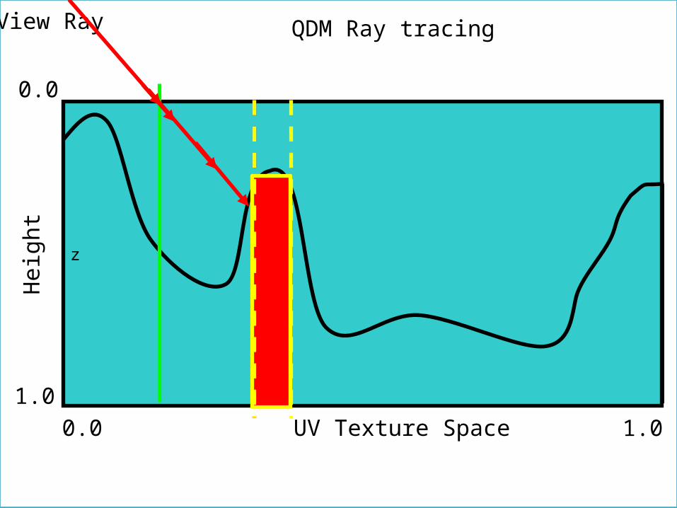
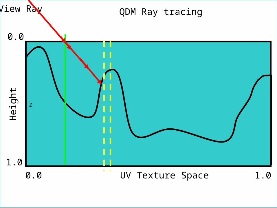
• Ray tracing– Traverse the quadtree
• From root (max MIP-hierarchy level)• To lowest leaf (MIP-hierarchy Level 0)
– MIP Level 0• Accurate intersection• Can get inter-texel results using
– Linear approximation– Binary Search– Bilinear Patch
Ray tracing
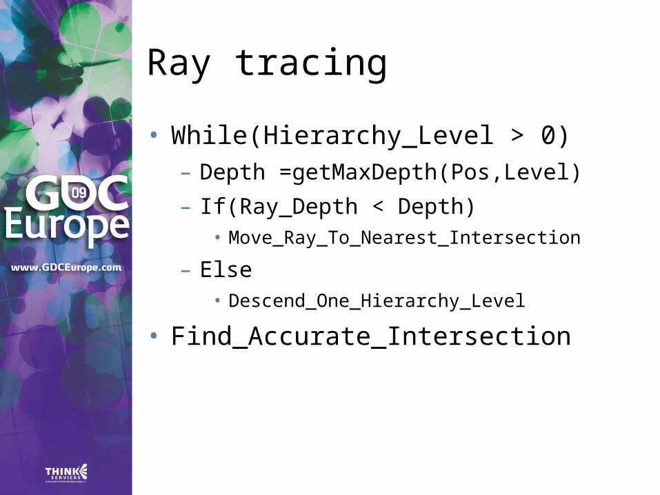
• While(Hierarchy_Level > 0)– Depth =getMaxDepth(Pos,Level)– If(Ray_Depth < Depth)
• Move_Ray_To_Nearest_Intersection
– Else• Descend_One_Hierarchy_Level
• Find_Accurate_Intersection
QDM construction
z
Heig
ht
0.0
0.01.0
1.0UV Texture Space
QDM construction
z
Heig
ht
0.0
0.01.0
1.0UV Texture Space
QDM construction
z
Heig
ht
0.0
0.01.0
1.0UV Texture Space
QDM construction
z
Heig
ht
0.0
0.01.0
1.0UV Texture Space

QDM construction
z
Heig
ht
0.0
0.01.0
1.0UV Texture Space

QDM construction
z
Heig
ht
0.0
0.01.0
1.0UV Texture Space
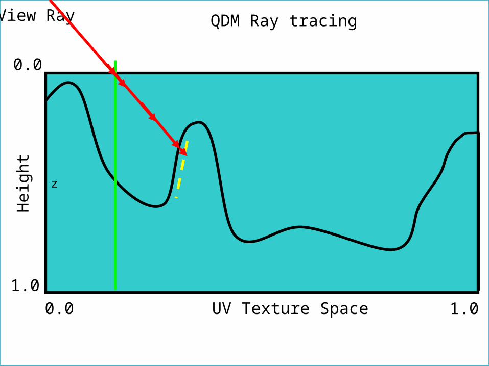
QDM Ray tracing
z
Heig
ht
0.0
0.01.0
1.0UV Texture Space
View Ray
QDM Ray tracing
z
Heig
ht
0.0
0.01.0
1.0UV Texture Space
View Ray

QDM Ray tracing
z
Heig
ht
0.0
0.01.0
1.0UV Texture Space
View Ray

QDM Ray tracing
z
Heig
ht
0.0
0.01.0
1.0UV Texture Space
View Ray

QDM Ray tracing
z
Heig
ht
0.0
0.01.0
1.0UV Texture Space
View Ray
QDM Ray tracing
z
Heig
ht
0.0
0.01.0
1.0UV Texture Space
View Ray
QDM Ray tracing
z
Heig
ht
0.0
0.01.0
1.0UV Texture Space
View Ray
QDM Ray tracing
z
Heig
ht
0.0
0.01.0
1.0UV Texture Space
View Ray
QDM Ray tracing
z
Heig
ht
0.0
0.01.0
1.0UV Texture Space
View Ray
QDM Ray tracing
• Algebraically perform intersection test between Ray, Cell boundary and minimum depth plane– Compute the nearest intersection and move the ray– In case of cell crossing choose the nearest one
• Ray is traversing through discrete data set– We must use integer math for correct ray position
calculation• SM 4.0 – accurate and fast• SM 3.0 – emulation and slower
– Point Filtering• LinearMipMapLinear is possible but may introduce some
artifacts– Trade samplers for artifacts– i.e. when using same texture for normal and depth storage
QDM Ray tracing
• Refinement– LEVEL 0 yields POINT discrete results– Depending on surface magnification and
need for inter-texel accuracy additional refinement method may be used• Binary Search
– Usable for non linear surfaces
• Linear piecewise approximation– Fast– Accurate due to approximation between 2 texels
only
• Bilateral Patch– most accurate for analytic surfaces– Requires additional memory– slow
QDM Ray tracing
• Fixed iteration count– Complexity O(log(n))
• Still may be prohibitive
– Set maximum iteration count
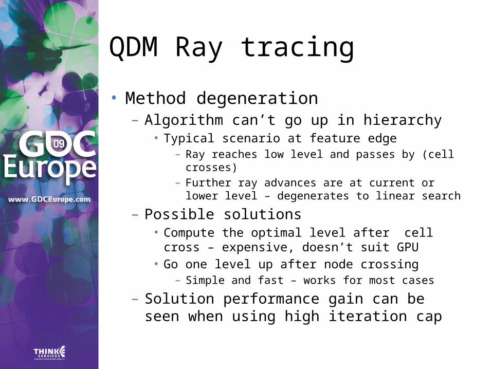
QDM Ray tracing
• Method degeneration– Algorithm can’t go up in hierarchy
• Typical scenario at feature edge– Ray reaches low level and passes by (cell
crosses)– Further ray advances are at current or lower
level – degenerates to linear search
– Possible solutions• Compute the optimal level after cell cross –
expensive, doesn’t suit GPU• Go one level up after node crossing
– Simple and fast – works for most cases
– Solution performance gain can be seen when using high iteration cap
QDM LOD
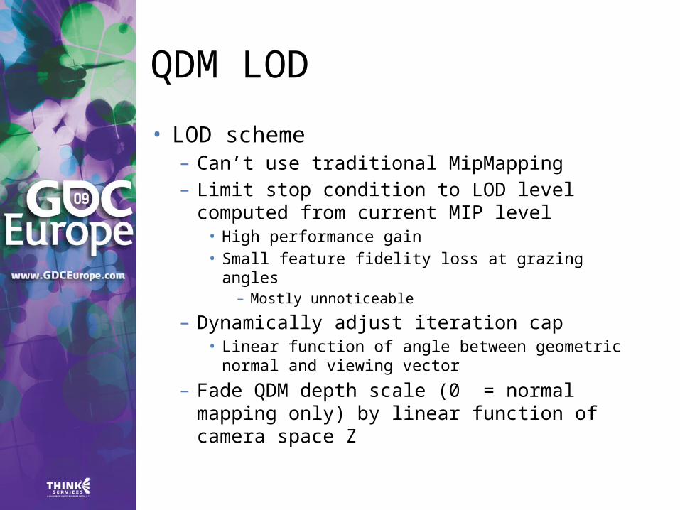
• LOD scheme– Can’t use traditional MipMapping– Limit stop condition to LOD level
computed from current MIP level• High performance gain• Small feature fidelity loss at grazing angles
– Mostly unnoticeable
– Dynamically adjust iteration cap• Linear function of angle between geometric
normal and viewing vector
– Fade QDM depth scale (0 = normal mapping only) by linear function of camera space Z
QDM Storage
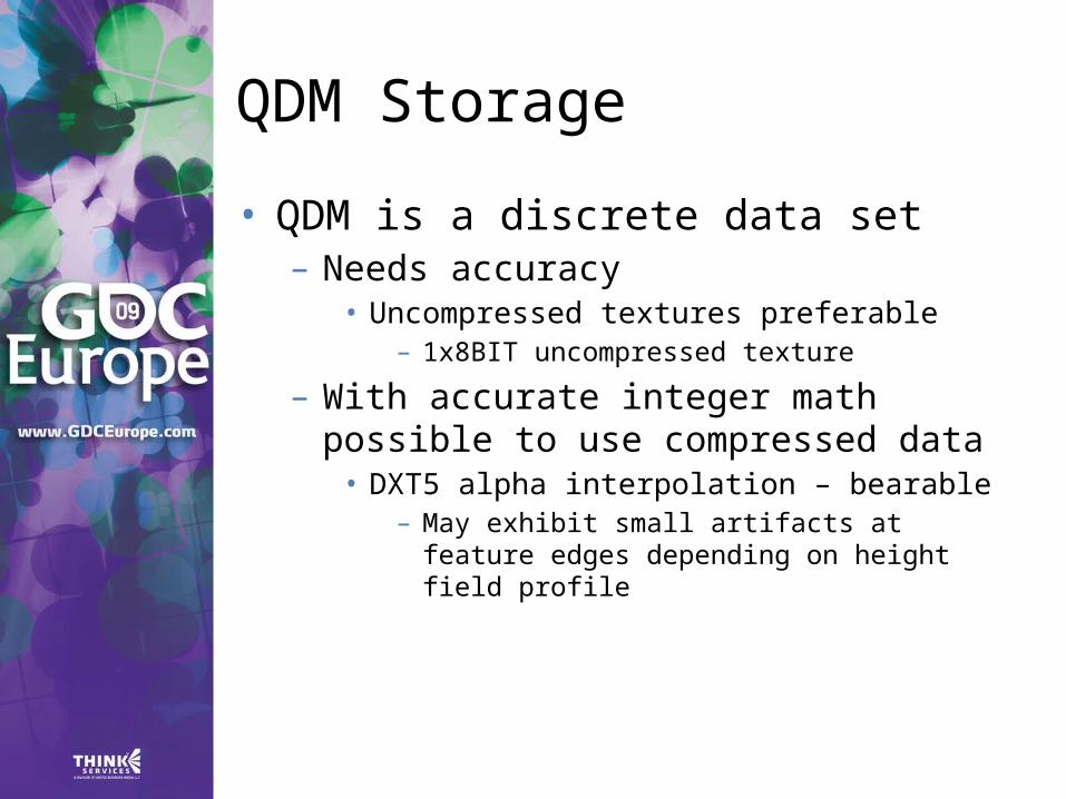
• QDM is a discrete data set– Needs accuracy
• Uncompressed textures preferable– 1x8BIT uncompressed texture
– With accurate integer math possible to use compressed data• DXT5 alpha interpolation – bearable
– May exhibit small artifacts at feature edges depending on height field profile
QDM
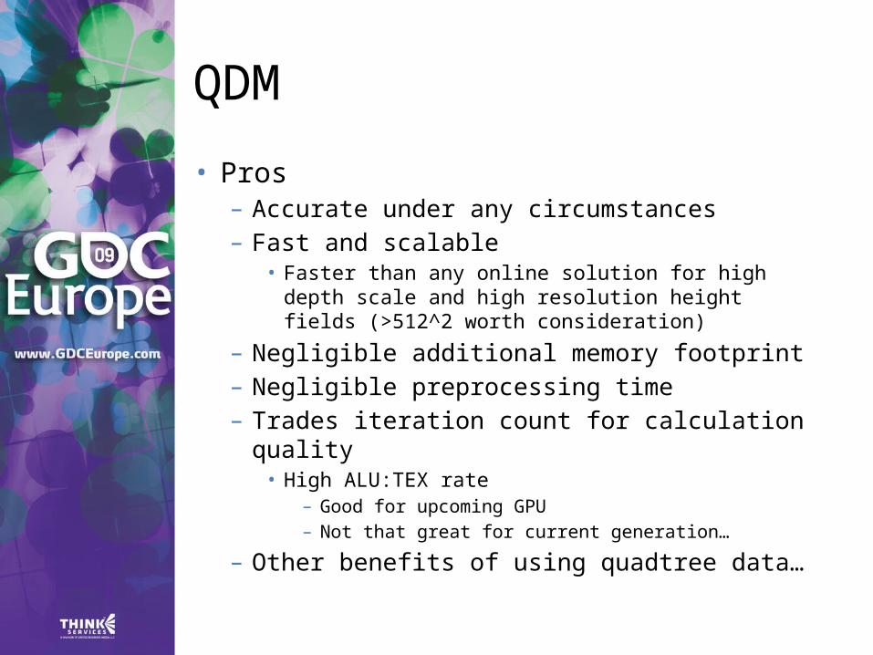
• Pros– Accurate under any circumstances– Fast and scalable
• Faster than any online solution for high depth scale and high resolution height fields (>512^2 worth consideration)
– Negligible additional memory footprint– Negligible preprocessing time– Trades iteration count for calculation quality
• High ALU:TEX rate– Good for upcoming GPU– Not that great for current generation…
– Other benefits of using quadtree data…
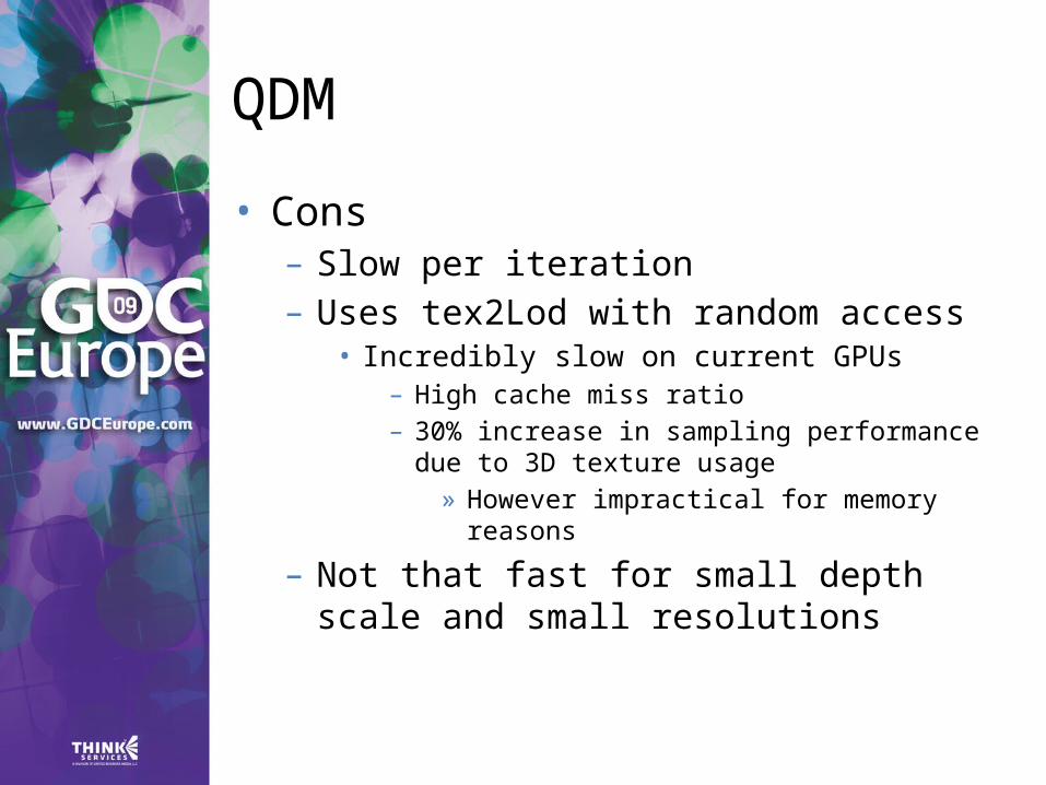
QDM
• Cons– Slow per iteration– Uses tex2Lod with random access
• Incredibly slow on current GPUs– High cache miss ratio– 30% increase in sampling performance
due to 3D texture usage» However impractical for memory
reasons
– Not that fast for small depth scale and small resolutions
Comparison
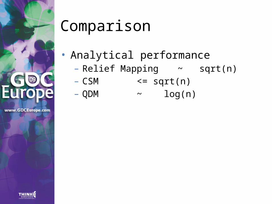
• Analytical performance– Relief Mapping ~ sqrt(n)– CSM <= sqrt(n)– QDM ~ log(n)
Comparison
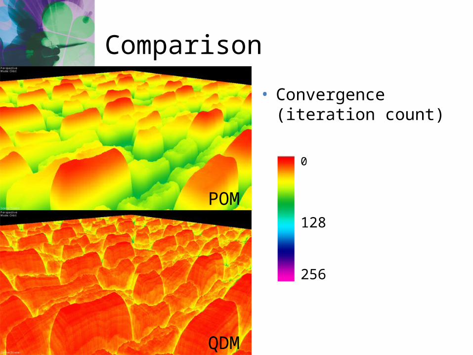
• Convergence (iteration count)
POM
QDM
0
256
128
Comparison
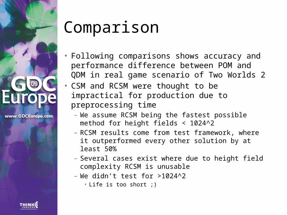
• Following comparisons shows accuracy and performance difference between POM and QDM in real game scenario of Two Worlds 2
• CSM and RCSM were thought to be impractical for production due to preprocessing time– We assume RCSM being the fastest possible
method for height fields < 1024^2– RCSM results come from test framework, where it
outperformed every other solution by at least 50%– Several cases exist where due to height field
complexity RCSM is unusable– We didn’t test for >1024^2
• Life is too short ;)
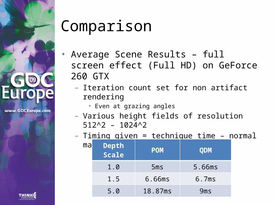
Comparison
• Average Scene Results – full screen effect (Full HD) on GeForce 260 GTX– Iteration count set for non artifact rendering
• Even at grazing angles
– Various height fields of resolution 512^2 – 1024^2
– Timing given = technique time – normal mapping time
Depth Scale POM QDM
1.0 5ms 5.66ms
1.5 6.66ms 6.7ms
5.0 18.87ms 9ms
QDM Depth Scale 1.0

POM Depth Scale 1.0
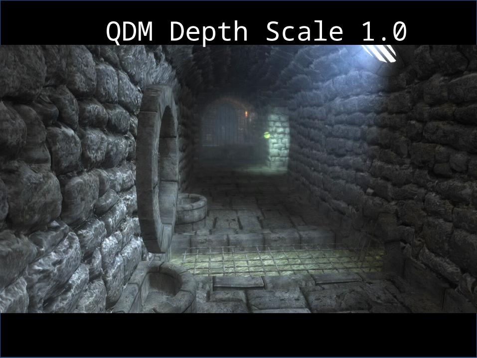
QDM Depth Scale 1.0
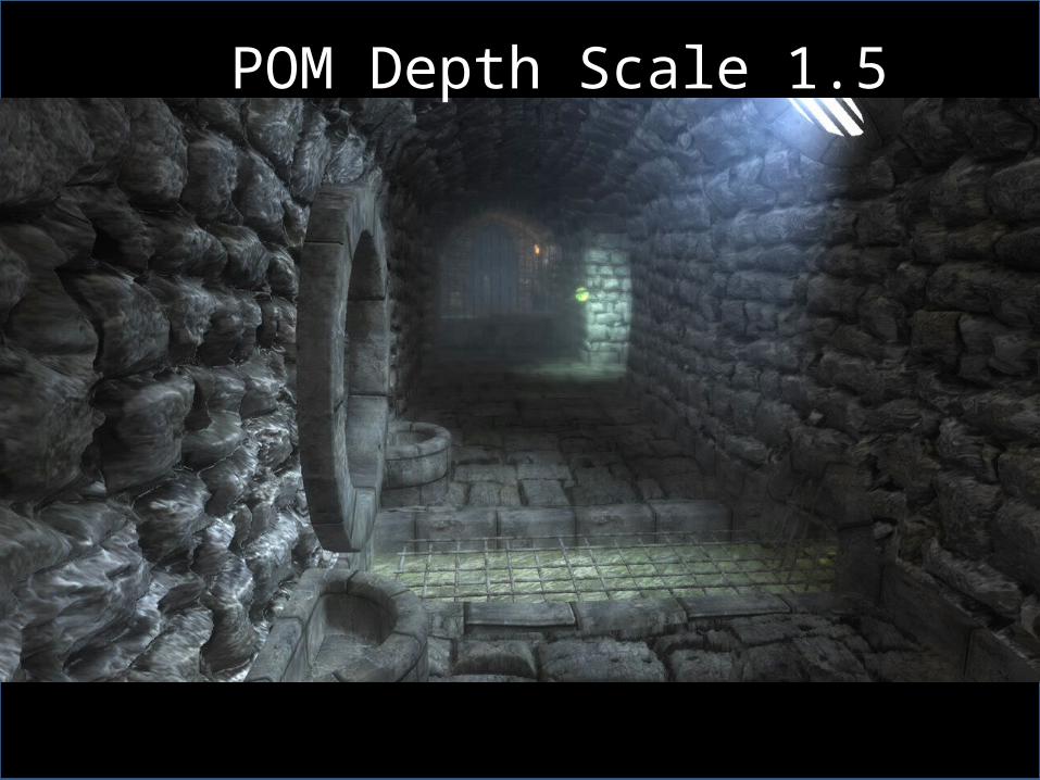
POM Depth Scale 1.5

QDM Depth Scale 1.5
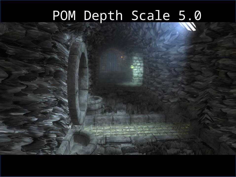
POM Depth Scale 5.0

QDM Depth Scale 5.0
Comparison
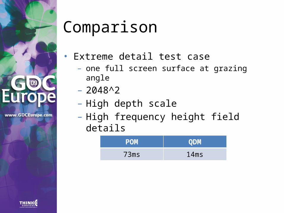
• Extreme detail test case – one full screen surface at grazing angle
– 2048^2– High depth scale– High frequency height field details
POM QDM
73ms 14ms
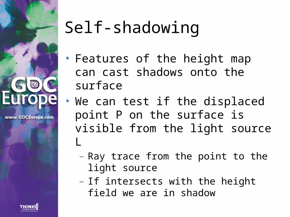
Self-shadowing
• Features of the height map can cast shadows onto the surface
• We can test if the displaced point P on the surface is visible from the light source L– Ray trace from the point to the light
source– If intersects with the height field we
are in shadow

Self-shadowingH
eig
ht
0.0
0.01.0
1.0UV Texture Space
View Ray
Light Ray
HIT – point in shadow
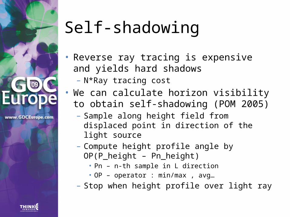
Self-shadowing
• Reverse ray tracing is expensive and yields hard shadows– N*Ray tracing cost
• We can calculate horizon visibility to obtain self-shadowing (POM 2005)– Sample along height field from displaced
point in direction of the light source– Compute height profile angle by
OP(P_height – Pn_height)• Pn – n-th sample in L direction• OP – operator : min/max , avg…
– Stop when height profile over light ray
Self-shadowing
• We can obtain soft shadows by filtering sampled values– Having blocker height we use linear
distance function to approximate penumbra size
• Algorithm complexity O(n)– n – number of height field texels along
given direction
• For performance reasons we limit sample count– Limits shadow effective length– Look out for aliasing

Self-shadowingPenumbra calculation
Heig
ht
0.0
0.01.0
1.0UV Texture Space
Light
Blocker Height
Self-shadowing
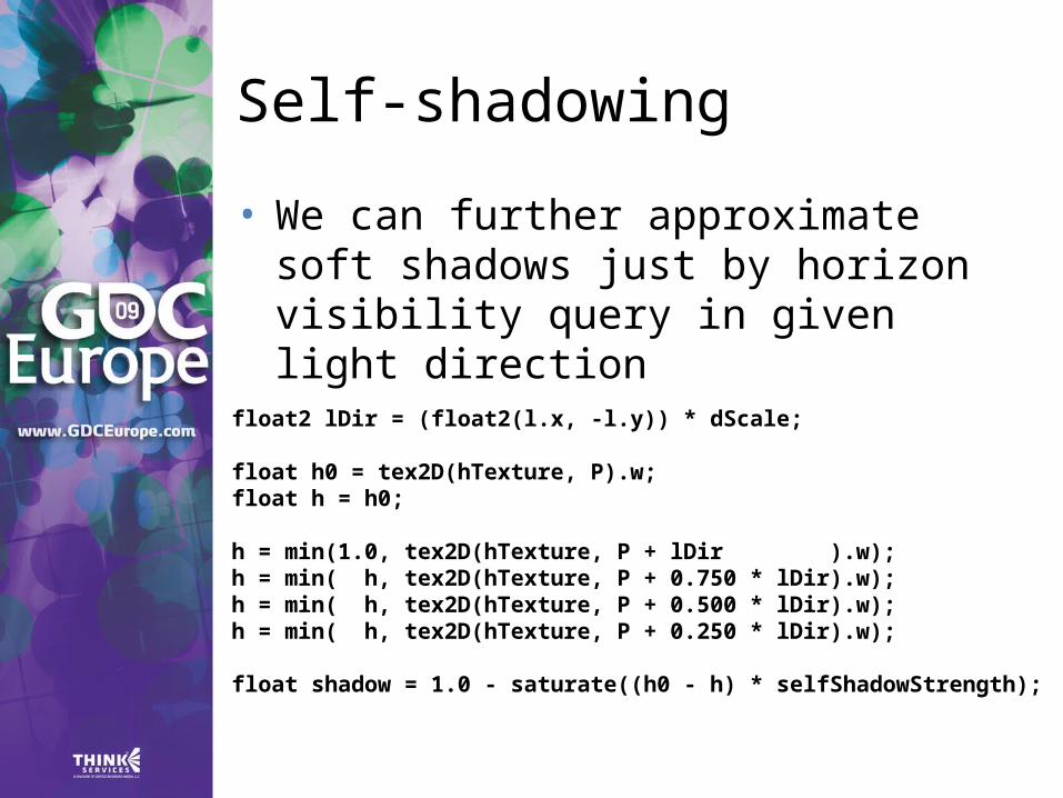
• We can further approximate soft shadows just by horizon visibility query in given light direction
float2 lDir = (float2(l.x, -l.y)) * dScale; float h0 = tex2D(hTexture, P).w; float h = h0; h = min(1.0, tex2D(hTexture, P + lDir ).w); h = min( h, tex2D(hTexture, P + 0.750 * lDir).w); h = min( h, tex2D(hTexture, P + 0.500 * lDir).w); h = min( h, tex2D(hTexture, P + 0.250 * lDir).w); float shadow = 1.0 - saturate((h0 - h) * selfShadowStrength);
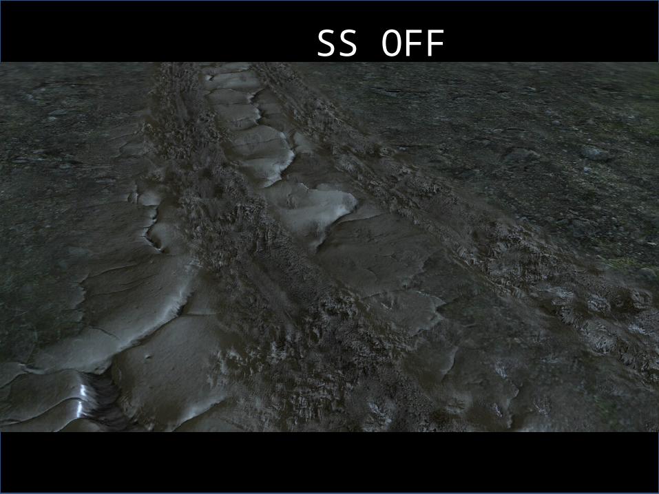
SS OFF
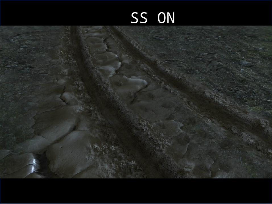
SS ON
QDM Self-shadowing
• Observation for light occlusion computation– Small scale details at distance have negligible
impact on the total occlusion outcome
• We can approximate further lying profile features using maximum height data from QDM– Minimize needed number of queries
• Full profile can be obtained in log(n) steps opposed to (n)
• We compute penumbra shadows by correct distance scaling of shadows
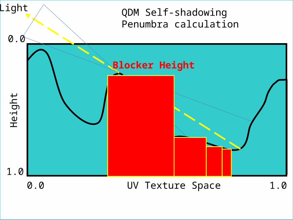
QDM Self-shadowingPenumbra calculation
Heig
ht
0.0
0.01.0
1.0UV Texture Space
Light
Blocker Height
QDM Self-shadowing
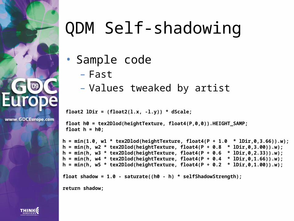
• Sample code– Fast– Values tweaked by artist
float2 lDir = (float2(l.x, -l.y)) * dScale;
float h0 = tex2Dlod(heightTexture, float4(P,0,0)).HEIGHT_SAMP; float h = h0;
h = min(1.0, w1 * tex2Dlod(heightTexture, float4(P + 1.0 * lDir,0,3.66)).w); h = min(h, w2 * tex2Dlod(heightTexture, float4(P + 0.8 * lDir,0,3.00)).w); h = min(h, w3 * tex2Dlod(heightTexture, float4(P + 0.6 * lDir,0,2.33)).w); h = min(h, w4 * tex2Dlod(heightTexture, float4(P + 0.4 * lDir,0,1.66)).w); h = min(h, w5 * tex2Dlod(heightTexture, float4(P + 0.2 * lDir,0,1.00)).w); float shadow = 1.0 - saturate((h0 - h) * selfShadowStrength); return shadow;

QDM Self-shadowing
• Self-shadowing– Adds depth– Quality– Moderate cost
• Full search only log(n)• Depends on shadow length (iteration cap)• Independent reads• Fast ALU• Full screen effect on test scene/machine
– 0.5ms

QDM SS OFF

QDM SS ON
Ambient Occlusion
• AO– Represents total light visibility for point
being lit– Adds depth– Can be computed and approximated
similarly to self shadowing• We perform several horizon occlusion queries
in different directions
– Need to calculate only when height field changes
– Especially useful for large scale terrain scenarios (i.e. darkening objects laying in a valley)
Ambient Occlusion
• Horizon queries– For each pixel perform horizon queries in const
n equally spaced directions and average results• Fast
– n*cost of horizon profile querying
• May need many directions– 4-12 shall work fine
– Can use jittering• For each pixel rotate directions by random• Can get away with 4 directions
– Uses dependant reads– Still better results than more directions
• Generally expensive– Use at content generation– If dynamic use time amortization
Surface Blending
• Used mainly in terrain rendering• Commonly by alpha blend – V = w * V1 + (1-w) * V2
• Blend weights typically encoded at vertex color– Weights being interpolated
• More accurate and flexible encoding blends in textures– Problematic– Large memory footprint
Surface Blending
• Alpha blending is not a good operator for surface blending– Surface exhibit more variety in
blends than simple gradients from per-vertex interpolation
– In real life surfaces don’t blend• What we see is actually the highest
material (or material being on top)• Rocks and sand – at blend we should see
rocks tops

Height Blending
• Height blending– Novel approach using height
information as additional blend coefficient
f1 = tex2Dlod(gTerraTex0Sampler, float4(TEXUV.xy, 0, Mip)).rgba; FinalH.a = 1.0 - f1.a; f2 = tex2Dlod(gTerraTex1Sampler, float4(TEXUV.xy, 0, Mip)).rgba; FinalH.b = 1.0 - f2.a; f3 = tex2Dlod(gTerraTex2Sampler, float4(TEXUV.xy, 0, Mip)).rgba; FinalH.g = 1.0 - f3.a; f4 = tex2Dlod(gTerraTex3Sampler, float4(TEXUV.xy, 0, Mip)).rgba; FinalH.r = 1.0 - f4.a;
FinalH*= IN.AlphaBlends;
float Blend = dot(FinalH, 1.0) + e; FinalH/= Blend; FinalTex = FinalH.a * f1 + FinalH.b * f2 + FinalH.g * f3 + FinalH.r * f4;

Blend Weights
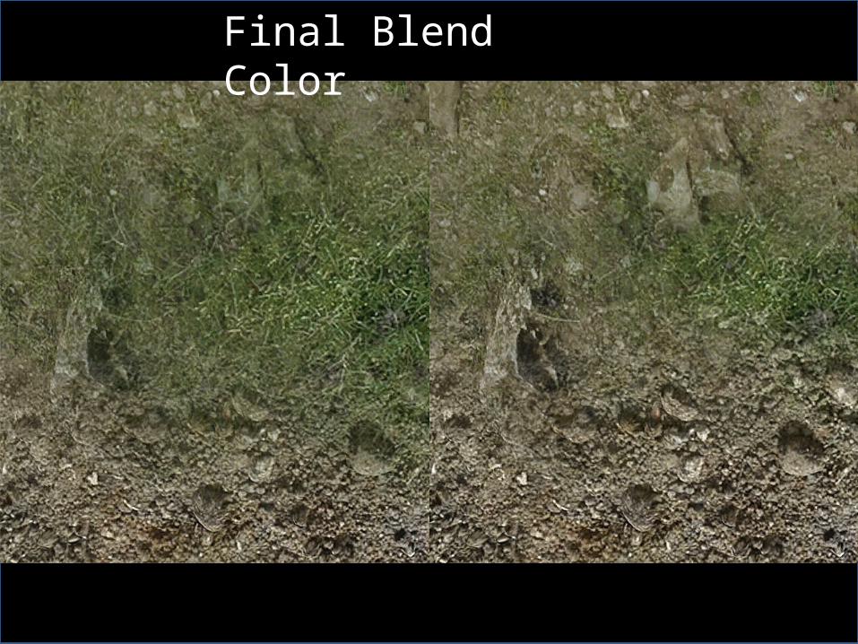
Final Blend Color
Height Blending
• HB– Adds variety– Cost is minimal
• Opposed to discussed methods
– Prefers the highest surface• Intersection search phase therefore needs
to find highest point only
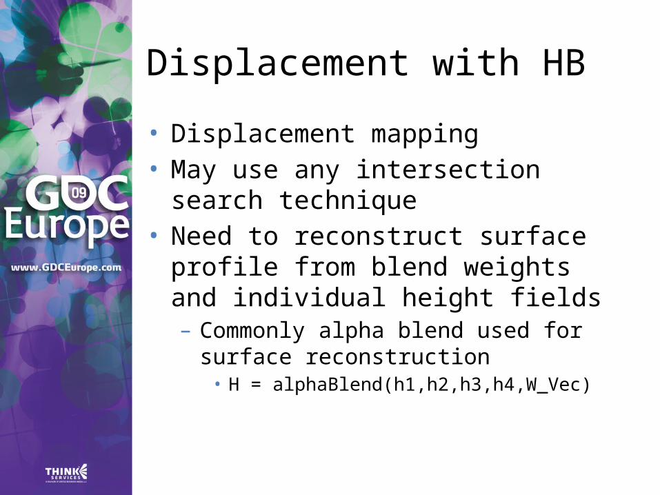
Displacement with HB
• Displacement mapping• May use any intersection search
technique• Need to reconstruct surface profile
from blend weights and individual height fields– Commonly alpha blend used for
surface reconstruction• H = alphaBlend(h1,h2,h3,h4,W_Vec)
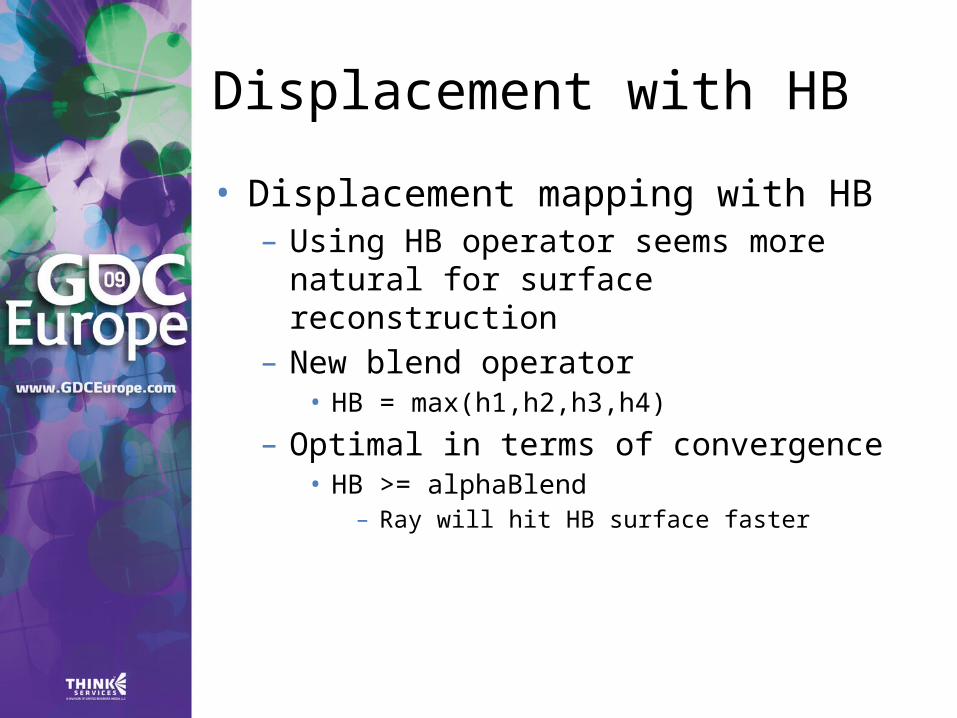
Displacement with HB
• Displacement mapping with HB– Using HB operator seems more
natural for surface reconstruction– New blend operator
• HB = max(h1,h2,h3,h4)
– Optimal in terms of convergence• HB >= alphaBlend
– Ray will hit HB surface faster
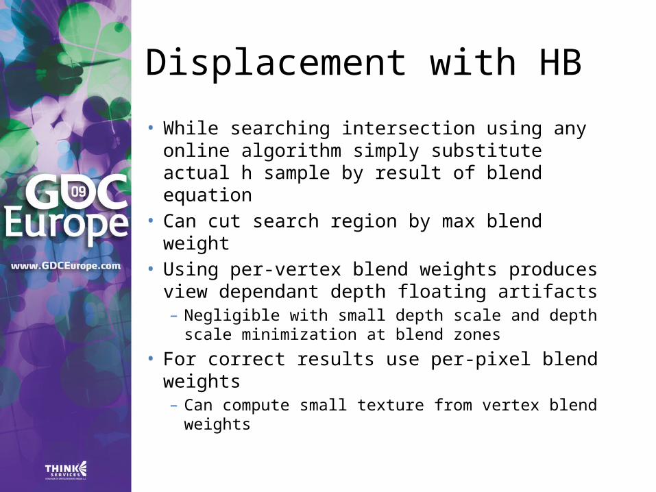
Displacement with HB
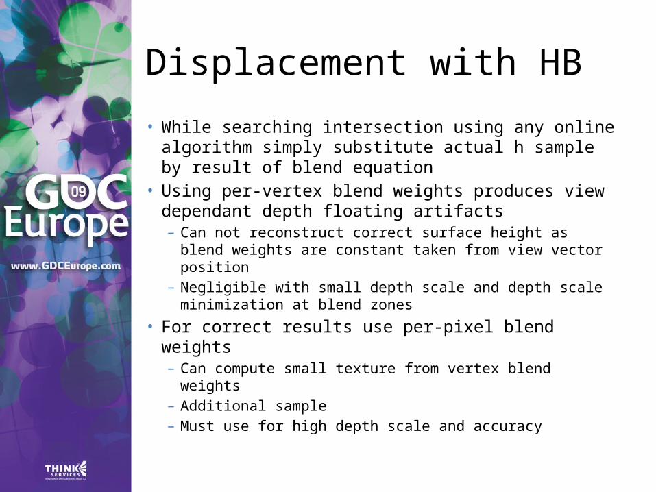
• While searching intersection using any online algorithm simply substitute actual h sample by result of blend equation
• Can cut search region by max blend weight
• Using per-vertex blend weights produces view dependant depth floating artifacts– Negligible with small depth scale and depth
scale minimization at blend zones
• For correct results use per-pixel blend weights– Can compute small texture from vertex blend
weights
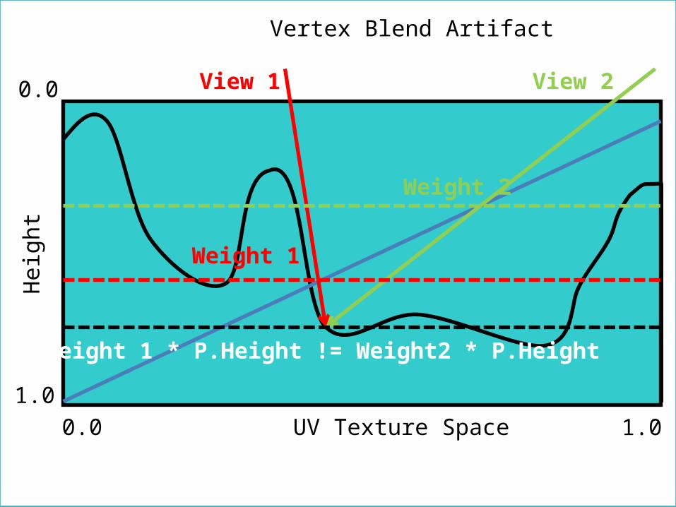
Displacement with HB
• While searching intersection using any online algorithm simply substitute actual h sample by result of blend equation
• Using per-vertex blend weights produces view dependant depth floating artifacts– Can not reconstruct correct surface height as blend
weights are constant taken from view vector position
– Negligible with small depth scale and depth scale minimization at blend zones
• For correct results use per-pixel blend weights– Can compute small texture from vertex blend
weights – Additional sample– Must use for high depth scale and accuracy
Vertex Blend ArtifactH
eig
ht
0.0
0.01.0
1.0UV Texture Space
View 1 View 2
Weight 2
Weight 1
Weight 1 * P.Height != Weight2 * P.Height
Displacement with HB
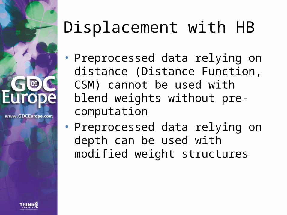
• Preprocessed data relying on distance (Distance Function, CSM) cannot be used with blend weights without pre-computation
• Preprocessed data relying on depth can be used with modified weight structures
QDM with HB
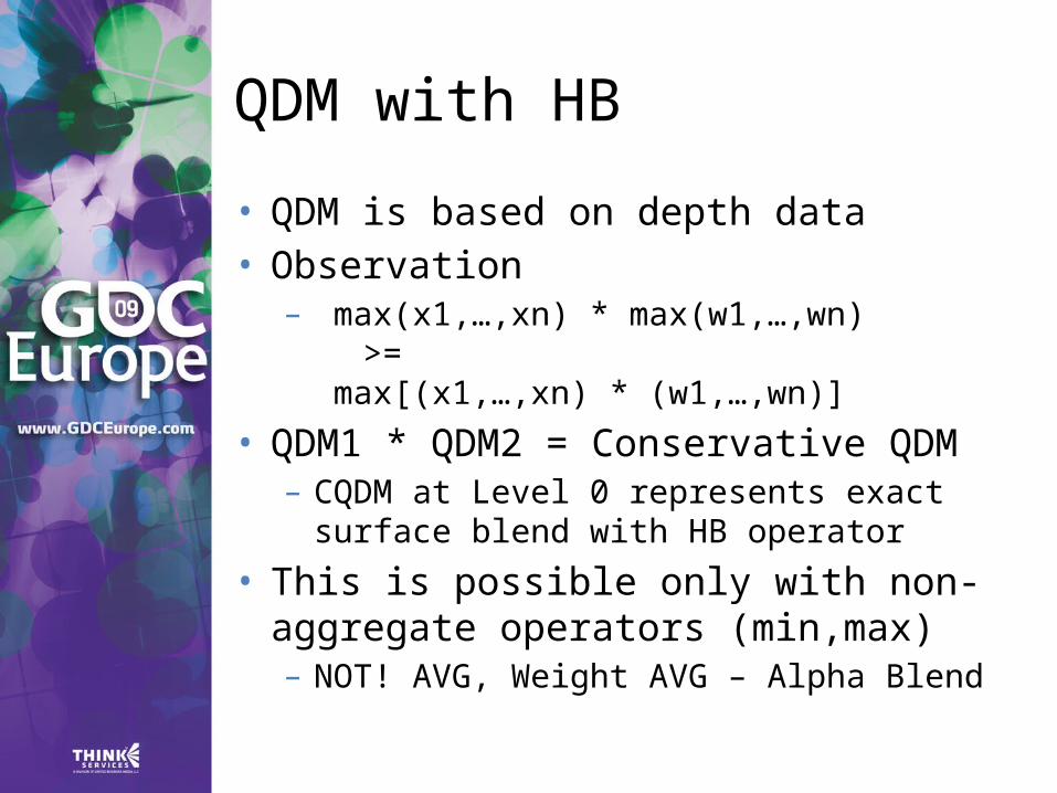
• QDM is based on depth data• Observation
– max(x1,…,xn) * max(w1,…,wn) >=
max[(x1,…,xn) * (w1,…,wn)]
• QDM1 * QDM2 = Conservative QDM– CQDM at Level 0 represents exact
surface blend with HB operator
• This is possible only with non-aggregate operators (min,max)– NOT! AVG, Weight AVG – Alpha Blend
QDM with HB
• QDMHB– Effectively we can use QDM with all its
benefits while blending surfaces for artifact free rendering
– Cons• On-the-fly / pre-computed Blend QDM
– Blend Texture from vertex– QDM from blend texture
• Conservative approach– Slower convergence– More iterations may be needed dependant
on field complexity– In practice <10% more iterations than
needed
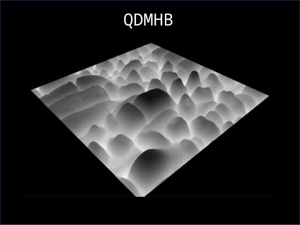
QDMHB
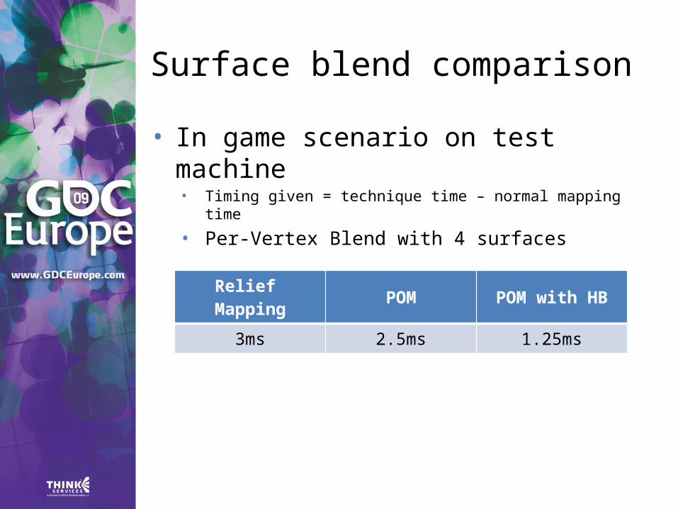
Surface blend comparison
• In game scenario on test machine• Timing given = technique time – normal mapping time
• Per-Vertex Blend with 4 surfaces
Relief Mapping POM POM with HB
3ms 2.5ms 1.25ms
Relief Mapping

POM Alpha Blend
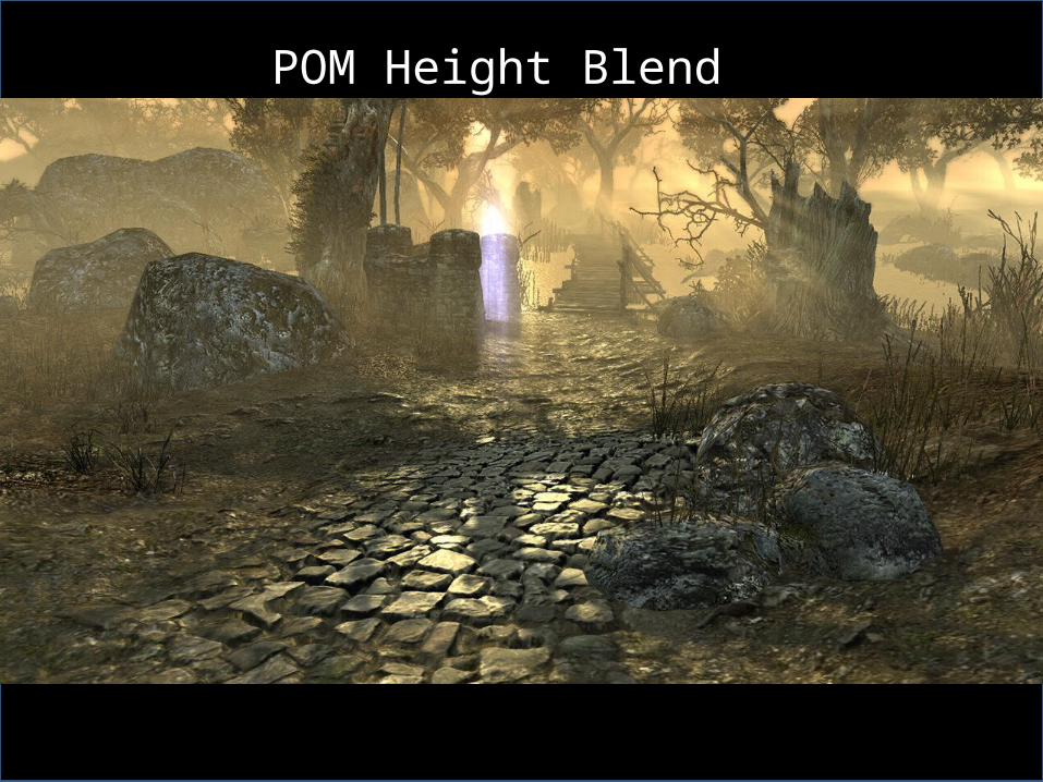
POM Height Blend
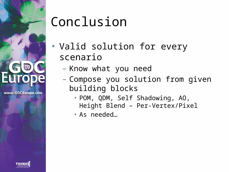
Conclusion
• Valid solution for every scenario– Know what you need– Compose you solution from given
building blocks• POM, QDM, Self Shadowing, AO, Height
Blend – Per-Vertex/Pixel• As needed…

Conclusion
• On limited hardware– Optimize as much as you can
• Terrain - fast low iteration POM with Per-Vertex HB, computed only for textures that really benefit
• Special Features – QDM with Soft Shadows• General Objects – use low iteration POM,
Soft Shadows at artist preference, check whether QDM is optimal for >1024^2
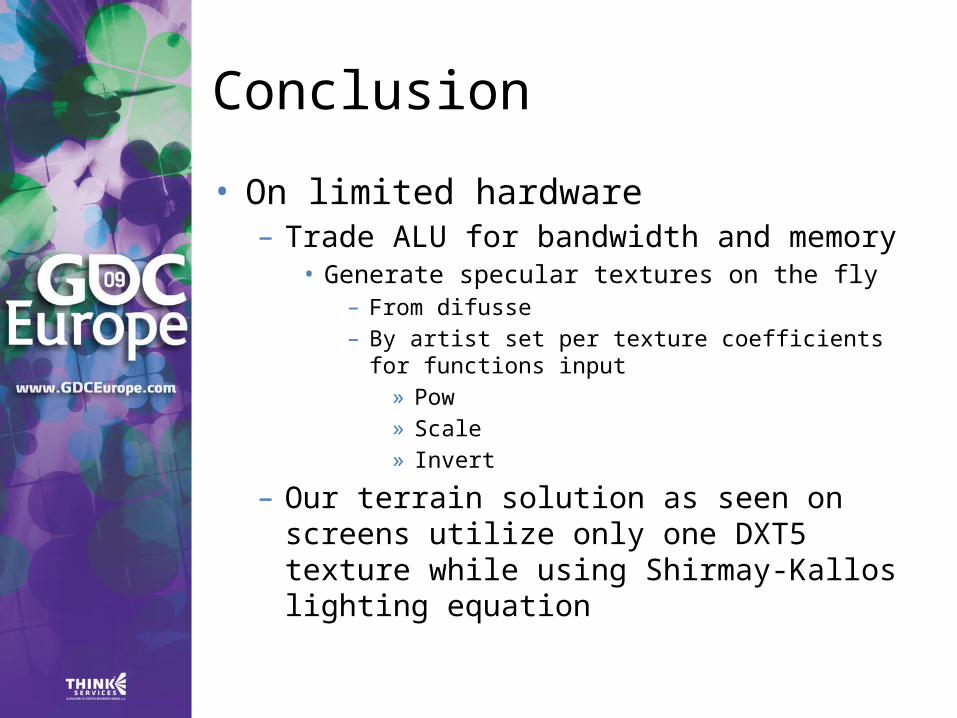
Conclusion
• On limited hardware– Trade ALU for bandwidth and memory
• Generate specular textures on the fly– From difusse– By artist set per texture coefficients for
functions input» Pow» Scale» Invert
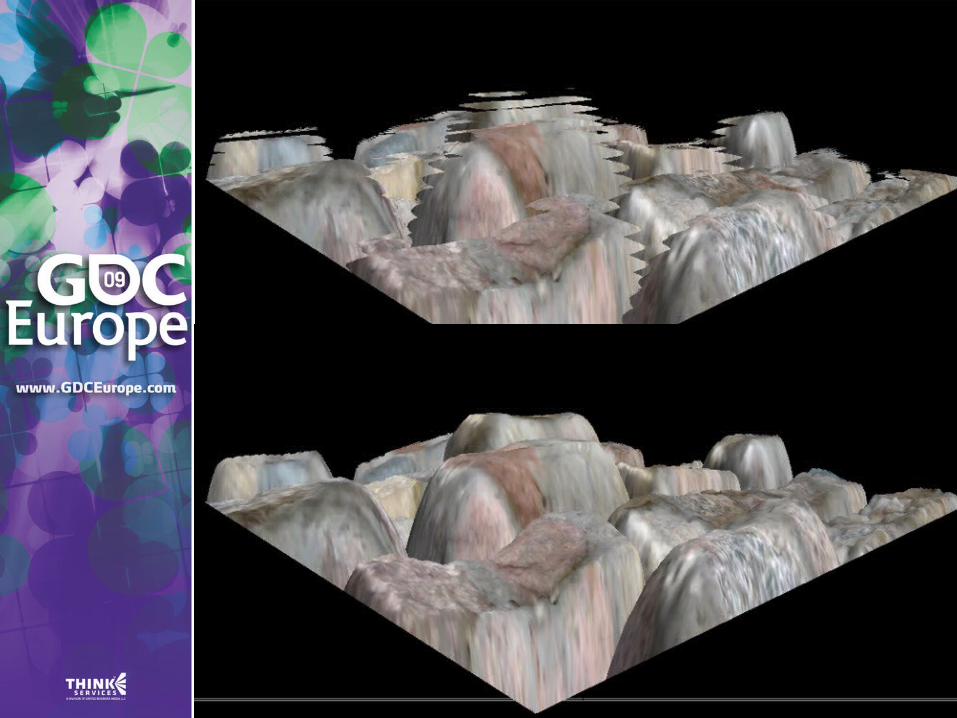
– Our terrain solution as seen on screens utilize only one DXT5 texture while using Shirmay-Kallos lighting equation

Conclusion
• Look out for future GPUs– Proposed high ALU methods will be
even more beneficial for new architecture
– Ray tracing vs tessalation ?• Will see…
• Happy surfacing!
Acknowledgements
• Reality Pump– especially Mariusz Szaflik – RP lead
programmer for continuous help in graphic struggles

Additional Info
• Additional information will be available in upcoming technical article, go to
• www.drobot.org – for details• [email protected]