qualitative reasoning for additional die casting …/67531/metadc736140/m2/1/high...qualitative...

QUALITATIVE REASONING FOR ADDITIONAL DIE CASTING APPLICATIONS

Project DE-FC07-98ID13690

FINAL REPORT

R. Allen Miller, Professor

Dehua Cui Yuming Ma

Industrial, Welding and Systems Engineering

Center for Die Casting The Ohio State Univerisity

210 Baker Systems Building 1971 Neil Avenue

Columbus, OH 43210 Phone: 614-292-7067 Fax: 614-292-7852

May 28, 2003

i

TABLE OF CONTENTS

Table of Contents .......................................................................................................................i Abstract .....................................................................................................................................v 1. Introduction ..........................................................................................................................1

1.1 Introduction ........................................................................................................................... 1 1.2 Design for Manufacturing and Geometric Reasoning........................................................... 2 1.3 Research Objective ....................................................................................................................... 3 1.4 Organization of the Report ................................................................................................. 4

2. Background ..........................................................................................................................5 2.1 Distortion Related Effects in Die Casting Process................................................................. 5

2.1.1 Dimensional Variation of Castings ................................................................................. 7 2.1.2 Ejectability............................................................................................................................ 9

2.2 The Factors That Influence to Casting Distortion............................................................... 12 Modeling of Dimensional Variation of Castings.................................................................. 12 Factor 1: Thermal Strain ........................................................................................................... 13 Factor 2: Elastic Strain............................................................................................................... 14 Factor 3: Inelastic stain.............................................................................................................. 15 Factor 4: Interaction with Die.................................................................................................. 15 Factor 5: Phase transformation................................................................................................ 15 Factor 6: Effect of Fluid Flow................................................................................................. 16

2.3 Numerical Simulation to Evaluate Casting Distortion ........................................................ 16 2.4 Qualitative Reasoning Approach ............................................................................................. 17

2.4.1 Early Manufacturability Evaluation............................................................................... 18 2.4.2 Interpretation of the Evaluation Results...................................................................... 19 2.4.3 Simple to use ..................................................................................................................... 20 2.4.4 High Efficiency ................................................................................................................. 20

2.5 Complementary of numerical simulation and qualitative approach.................................. 21 2.5.1 Performing Quantitative Approach and Numerical Simulation at Different Periods of Product Development ............................................................................................................... 21 2.5.2 Performing Quantitative Evaluation before Numerical Simulation ....................... 22 2.5.3 Performing Quantitative Evaluation and Numerical Simultaneously..................... 22

3. Qualitative Reasoning of Casting distortion .....................................................................23 3.1 Introduction ................................................................................................................................. 23 3.2 Laplace’s Equation and Volume Potential Theory............................................................... 23

3.2.1 Potential Theory ............................................................................................................... 25 3.2.2 Asymptotic Expression for the Volume Potential ..................................................... 26

3.3 Volume Potential and Body Force Analogy of Thermoelastic Problems........................ 29 3.3.1 Thermal stress analysis and body force analogy ......................................................... 32 3.3.2 Body Force Analogy......................................................................................................... 32 3.3.3 Potential Theory to Solve Thermoelastic Boundary-value Problems..................... 34 3.3.4 Saint Venant’s Principle................................................................................................... 36

ii

3.4 Temperature Reasoning............................................................................................................. 36 3.4.1 The Correlation between Temperature and Wall Thickness of Castings .............. 37 3.4.2 The Correlation between Heat Trap in Die and Wall Thin Section of Casting die38 3.4.3 Qualitative Evaluation of Temperature Distribution ................................................ 39

3.5 Free shrinkage.............................................................................................................................. 43 3.5.1 Thermal Skeleton and Shrinkage Center...................................................................... 45 3.5.2 Free Shrinkage Pattern..................................................................................................... 48

3.6 Constrained Shrinkage ............................................................................................................... 49 3.6.1Constrained Shrinkage Pattern........................................................................................ 51 3.6.2 Extraction of constrained Surfaces ............................................................................... 51

4. Thermal Plastic Distortion Reasoning...............................................................................53 4.1 Introduction ................................................................................................................................. 53 4.2 Stress-Strain Curve Constitutive Approach ........................................................................... 53

4.2.1 Qualitative Reasoning of the Plastic Behavior ............................................................ 54 4.2.2 Qualitative Reasoning for Thermal Plastic Distortion .............................................. 56

4.3 Effect estimation of the thermal plastic distortion in die casting ...................................... 58 4.4 Summary....................................................................................................................................... 60

5. Geometric Reasoning For Casting distortion....................................................................61 5.1 Introduction ................................................................................................................................. 61 5.2 Part Model.................................................................................................................................... 61 5.3.Distance Transform.................................................................................................................... 63

5.3.1 Double Stack City block Distance Transform............................................................ 65 5.3.2 Two Pass Euclidean distance Transforms ................................................................... 66 5.3.3 Double Stack Euclidean Distance Transform Algorithm......................................... 71 5.3.4 Extraction of the Distance-Based Skeleton................................................................. 73

5.4 Calculation of Distortion Patterns........................................................................................... 75 5.4.1 Calculation of Free Shrinkage Pattern .......................................................................... 76 5.4.2 Extraction of Constrained Surfaces .............................................................................. 78 5.4.3 Calculation of Constrained Shrinkage Pattern ............................................................ 79 5.4.4 Temperature Pattern ........................................................................................................ 80

5.5 Plastic Distortion Pattern .......................................................................................................... 84 5.5.1 Contextual Distortion...................................................................................................... 85 5.5.2 Plastic Distortion Pattern................................................................................................ 87

5.6 Summary....................................................................................................................................... 88 6. The Evaluation of Ejectability of Casting by Geometric Reasoning ...............................89

6.1 Introduction ................................................................................................................................. 89 6.2 Evaluation of Ejectability .......................................................................................................... 90

6.2.1 Constrained Surface and Limited Draft Surfaces ....................................................... 90 6.2.2 Ejection Pattern and Ejection Resistance of Constrained Voxels .......................... 91 6.2.3 Pin’s Relative Ejection Force Rating............................................................................. 92 6.2.4 Ejection moment .............................................................................................................. 93 6.2.5 The ratio of ejection load on ejector die to ejection load on cover die.................. 94 6.2.6 Evaluation tool for ejector pin layout........................................................................... 94

6.3 Summary....................................................................................................................................... 95 7. Verification ........................................................................................................................96

7.1 Introduction ................................................................................................................................. 96

iii

7.2 Comparisons between Temperature Reasoning and Numerical Simulation Results..... 96 Case Study 1: Special cases with known temperature distributions.................................. 96 Case Study 2: Flat plate part ................................................................................................... 103 Case Study 3: Collector Ring.................................................................................................. 107

7.3. Comparison Between Plastic Distortion Reasoning and Numerical Simulation......... 112 7.4 Ejectability Case Studies .......................................................................................................... 116

Case Study 4: Ejector pin Design Example......................................................................... 116 Case Study 5: Industrial Part with Suspicious Ejection Defects...................................... 123

7.5 Industrial case study ................................................................................................................. 127 8. Conclusions ......................................................................................................................130

8.1 Summary of Research Contribution...................................................................................... 130 8.2 Suggestion for Future Work ................................................................................................... 131

References .............................................................................................................................133

v

ABSTRACT

If manufacturing incompatibility of a product can be evaluated at the early product design stage, the designers can modify their design to reduce the effect of potential manufacturing problems. This will result in fewer manufacturing problems, less redesign, less expensive tooling, lower cost, better quality, and shorter development time. For a given design, geometric reasoning can predict qualitatively the behaviors of a physical manufacturing process by representing and reasoning with incomplete knowledge of the physical phenomena. It integrates a design with manufacturing processes to help designers simultaneously consider design goals and manufacturing constraints during the early design stage. The geometric reasoning approach can encourage design engineers to qualitatively evaluate the compatibility of their design with manufacturing limitations and requirements.

Casting distortion not only influences the quality of the product but also the manufacturing procedure of a die-casting. Casting distortion problems can be reduced during part design. By evaluating the distortion tendencies of a given design, the designers can modify their design to reduce these effects and reduce manufacturing problems. A geometric reasoning approach has been developed to qualitatively evaluate casting distortion. The geometric reasoning can predict the casting distortion pattern based on the geometric and topologic information of the design. In addition, it can extract the design characteristics that cause the distortion-related problems. The results of the geometric reasoning can be used to support the ejectability evaluation for a given casting design and the ejector pin layouts. Through geometric reasoning, the constrained surfaces are determined and the ejection load developed on them is qualitatively evaluated based on the geometric and topologic information describing the part. In addition, several evaluation functions, such as the effective relative ejection force rating of each ejector pin, ejection moment, ejection pattern, the ratio of the ejection load on the ejector die to that on cover die, are defined and evaluated.

The information obtained from the reasoning can give casting designers manufacturability feedback about their design and will help them make design decisions to reduce the potential manufacturing defects related to casting distortion. In addition, the information obtained from the reasoning can give die designers an evaluation about their ejector pin design and will help them make design decisions in locating ejector pins and orienting the part in the die to reduce the ejection-related defects.

1

1. INTRODUCTION

1.1 Introduction

Making products more quickly and efficiently is even more important in these times of increasing economic competition. When a design is passed to manufacturing engineers without proper evaluation, manufacturing difficulties could arise so that the design would have to be returned to the designers for modifications. To avoid this laborious, costly, and time-consuming design iteration, early analysis and detection of possible manufacturing problems is essential. Existing CAE system often provide numerical simulation facilities for checking designs. However, a numerical simulation is ineffectual in the early stage of a design because too little is known about the design and the manufacturing process. In the later stages, numerical simulation can be used, but any serious problems uncovered then often are fixed only at greatly increased expense, both in term of designer time and computer time. Aside from the ability to catch blunders early, knowing early in the design process what undesirable behaviors might be exhibited can allow the posting of constraints in other choices in the design, in order to prevent such possibilities from occurring.

During the die casting process a colder die is filled with hot molten material which then cools and solidifies. As the material cools and solidifies, it will shrink. The shrinkage of castings will result in casting distortion, the shape and size of castings deviating from the desired and nominal dimensions. For some casting features where normal shrinkage cannot take place due to resistance of the die wall, non-uniform shrinkage will be developed. These casting surfaces whose shrinkage are constrained by die walls are referred to as ‘constrained surfaces’. Since normal shrinkage cannot take place, equivalent internal stress develops as the casting cools from its solidification temperature to its ejection temperature. This results in an ejection load on the constrained surfaces. This ejection load creates an ejection resistance during the ejection operation of die casting process. With the help of the ejector pins, the ejection load acting on the constrained surfaces of castings will be released and the casting then is pushed off the die ejector surface. The position, number and size of ejector pins must be carefully planned to overcome the resistance to ejection. The geometric characteristics and the ejection load of castings play important roles in determining the ejector pin’s number, location, size, shape, and distribution (Herman,1985). Consequently, casting distortion not only influences the quality of the product but also the die casting procedure.

2

A high quality die and die casting part design should insure that the castings will be ejected readily from the die without defects, require the least die construction and maintenance work, and meet the specified tolerance requirements(Sully 1978; Herman 1985). However, in the past, the die casting industry has had a high incidence of failures (Herman,1985). Sometimes the failure is the inability to hold a dimensional tolerance. Other times scrap rates are excessive. Frequently, the die will just not operate. Leader pins stick, or cores will not register. These occurrences become catastrophic failures and it is too late for the designer to make modifications. Invariably some of these failures can be traced back to inadequate distortion and ejectability analyses during or before the product design and/or the die design stage. Proper modification and reasonably creative mechanics will invent solutions once the problems are recognized.

1.2 Design for Manufacturing and Geometric Reasoning

Design for manufacturability (DFM) has been introduced to reduce the functional gap between the design and manufacturing. DFM can be described as designing a product in a way that makes it easier to manufacture. Specifically, DFM is a design-evaluation technique that considers many diverse factors to give designers an indication of the quality of a candidate product design. If manufacturing incompatibility of a product can be evaluated at the early product design stage, the designers can modify their design to reduce the manufacturing problem. This will result in fewer manufacturing problems, less redesign, less expensive tooling, lower cost, better quality, and shorter development time. Contemporary computer-based design tools provide a sound technique for geometry creation and manipulation. However, they do not directly support manufacturing-related information processing and decision-making. Existing computer aided engineering systems often provide numerical simulation facilities for checking casting designs (Campbell,1993). However, a numerical simulation is ineffectual in the early stage of designer because too little is known about the die, process and operating conditions. The designed parts usually have complicated geometry, and the knowledge of manufacturing processes is very complicated and difficult to apply. In addition, the evaluation results are highly dependent on the part’s complexity and the designers’ knowledge and experience (Cross, 1993)(Thomas, 1993). On the other hand, some die-casting handbooks provide casting and casting die design guidelines, such as Herman (Herman,1985) has summarized a list of design guidelines to help designers and engineers choose an appropriate ejector pin location. Unfortunately, it is not enough to only follow these rules to establish good casting designs and casting die designs and significant effort and experience are required to understand, interpret, and apply these guidelines. For example, because some of the key factors that determine position, number, size, shape of ejector pins are not considered in these rules for ejector pin design, such as ejection load, constrained surfaces and their interaction, die open direction. Besides, identifying the limited draft surfaces, the constrained surfaces where these rules are individually applied, is not an easy task because of the complexity of castings and the interaction between the constrained surfaces.

Geometric reasoning is one of the DFM design evaluation techniques that integrates a design with manufacturing processes to help designers simultaneously consider design goals and manufacturing constraints during the early design stage. Geometric reasoning to qualitatively

3

evaluate the manufacturability of a product design can be introduced to reduce the functional gap between the design and manufacturing. For a given design, the qualitative approach can predict the behaviors of a physical process the manufacturing process involved by representing and reasoning with incomplete knowledge of the physical phenomena. It integrates a design with manufacturing processes to help designers simultaneously consider design goals and manufacturing constraints during the early design stage. The geometric reasoning approach can encourage design engineers to evaluate the compatibility of their design with manufacturing limitations and requirements.

1.3 Research Objective

The casting distortion not only influences the quality of the product but also the manufacture procedure of the die-casting. The goal of this research is to develop a geometric reasoning approach to qualitatively evaluate casting distortion. Through geometric reasoning, the casting distortion pattern of a casting design can be predicted based on the geometric and topologic information. Also the design characteristics that cause the distortion-related problems can be extracted. The information obtained from the reasoning can give casting designers additional feedback about their design and will help them make design decisions to reduce the effects of casting distortion. The information can also help die designers locate ejector pins and orient the part in the die.

The research objective can be broken down into the following major tasks:

1. Locate design entities that have significant influence on casting distortion-related problems. The constraint surfaces of a casting that cause non-uniform shrinkage, internal stress, and mechanical load on the wall of the casting will be extracted.

2. Qualitatively estimate general distortion patterns for a given casting design. The geometric reasoning approach will be developed so that the casting’s temperature distribute pattern, free shrinkage pattern, constrained distortion pattern, and plastic distortion pattern can be qualitative evaluated. With the distortion patterns, the dimensional variation, internal stress, and ejection load caused by casting distortion can be judged based on qualitative evaluation.

3. Develop a visualization tool to evaluate the ejectability effectiveness of ejector pin layouts based on the geometric reasoning of thermal distortion. The evaluation functions will be defined so that the ejectability can be evaluated. With the evaluation functions, the relative ejection force that each ejector pin should provide, the ejection moment that an ejector pin layout could create on the casting, the ratio of ejection load on ejector die to the cover die. The tool should be able not only evaluate the ejectability of a given ejector pin layout design but also give redesign recommendations.

4

The qualitative approach should be robust, conservative, complete, and efficient without providing misleading results. It should be able to deal with different part designs regardless of their shape and complexity. Finally, it should be efficient, fast, and easy to use.

It should also be noted that while the proposed qualitative evaluation is for the die casting process, it could also be used in other net shape manufacturing processes, such as injection molding, sand casting etc.

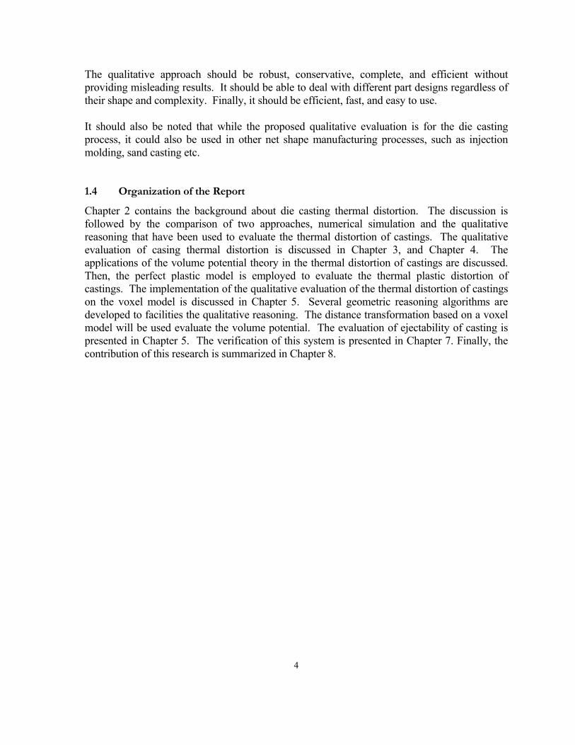
1.4 Organization of the Report

Chapter 2 contains the background about die casting thermal distortion. The discussion is followed by the comparison of two approaches, numerical simulation and the qualitative reasoning that have been used to evaluate the thermal distortion of castings. The qualitative evaluation of casing thermal distortion is discussed in Chapter 3, and Chapter 4. The applications of the volume potential theory in the thermal distortion of castings are discussed. Then, the perfect plastic model is employed to evaluate the thermal plastic distortion of castings. The implementation of the qualitative evaluation of the thermal distortion of castings on the voxel model is discussed in Chapter 5. Several geometric reasoning algorithms are developed to facilities the qualitative reasoning. The distance transformation based on a voxel model will be used evaluate the volume potential. The evaluation of ejectability of casting is presented in Chapter 5. The verification of this system is presented in Chapter 7. Finally, the contribution of this research is summarized in Chapter 8.

5

2. BACKGROUND

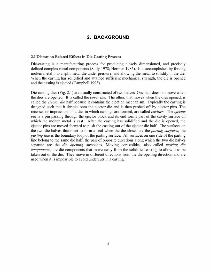
2.1 Distortion Related Effects in Die Casting Process

Die-casting is a manufacturing process for producing closely dimensioned, and precisely defined complex metal components (Sully 1978; Herman 1985). It is accomplished by forcing molten metal into a split metal die under pressure, and allowing the metal to solidify in the die. When the casting has solidified and attained sufficient mechanical strength, the die is opened and the casting is ejected (Campbell 1993).

Die-casting dies (Fig. 2.1) are usually constructed of two halves. One half does not move when the dies are opened. It is called the cover die. The other, that moves when the dies opened, is called the ejector die half because it contains the ejection mechanism. Typically the casting is designed such that it shrinks onto the ejector die and is then pushed off by ejector pins. The recesses or impressions in a die, in which castings are formed, are called cavities. The ejector pin is a pin passing through the ejector block and its end forms part of the cavity surface on which the molten metal is cast. After the casting has solidified and the die is opened, the ejector pins are moved forward to push the casting out of the ejector die half. The surfaces on the two die halves that meet to form a seal when the die closes are the parting surfaces; the parting line is the boundary loop of the parting surface. All surfaces on one side of the parting line belong to the same die half; the pair of opposite directions along which the two die halves separate are the die opening directions. Moving cores/slides, also called moving die components, are die components that move away from the solidified casting to allow it to be taken out of the die. They move in different directions from the die opening direction and are used when it is impossible to avoid undercuts in a casting.

6

Parting SurfaceEjector Die

Moving CoreCavity

Cover Die

Die OpeningDirection

Parting Line

Figure2.1: Die Casting Die Terminology (Adapted from “Designing For Thin Wall Zinc Die Castings”, International Lead Zinc Research Organization, Inc.)

Figure 2.2: Total dimensional variation of the casting increases with each stage in the process (Herman 1985).

7

2.1.1 Dimensional Variation of Castings

All dimensions of a casting are subject to linear variation (Herman1985). Linear variation describes the uniform dimensional variation. A casting feature that is formed completely in one die component (i.e. core, cover cavity, or ejector cavity) and can freely shrink can be assumed to subject linear dimensional variation only. Figure 2.2 illustrates the relative influence of normal fluctuations in die temperature, casting ejection temperature, quenching rate, and stress relieving heat treatment for a casting feature that can free shrink inside the die and be formed completely in one die half. The linear variation scale is sensitive and is therefore shown in terms of in./in. (mm/mm).

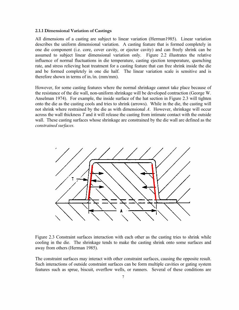
However, for some casting features where the normal shrinkage cannot take place because of the resistance of the die wall, non-uniform shrinkage will be developed contraction (George W. Anselman 1974). For example, the inside surface of the hat section in Figure 2.3 will tighten onto the die as the casting cools and tries to shrink (arrows). While in the die, the casting will not shrink where restrained by the die as with dimensional A. However, shrinkage will occur across the wall thickness T and it will release the casting from intimate contact with the outside wall. These casting surfaces whose shrinkage are constrained by the die wall are defined as the constrained surfaces.

Figure 2.3 Constraint surfaces interaction with each other as the casting tries to shrink while cooling in the die. The shrinkage tends to make the casting shrink onto some surfaces and away from others (Herman 1985).

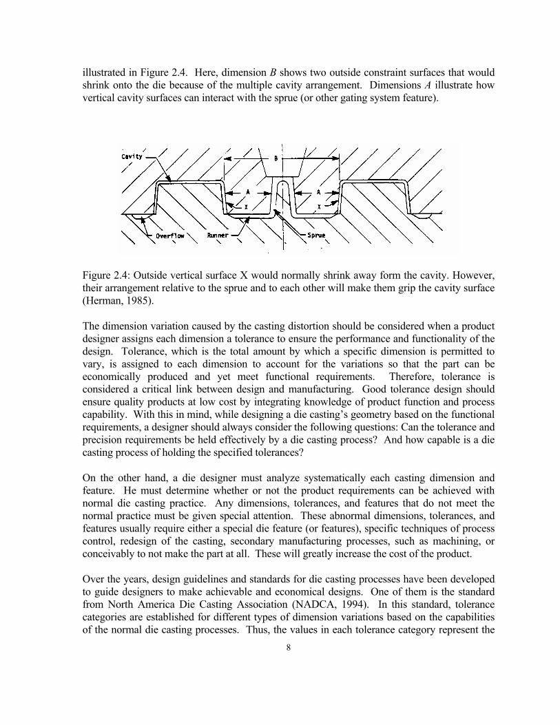
The constraint surfaces may interact with other constraint surfaces, causing the opposite result. Such interactions of outside constraint surfaces can be form multiple cavities or gating system features such as sprue, biscuit, overflow wells, or runners. Several of these conditions are

8

illustrated in Figure 2.4. Here, dimension B shows two outside constraint surfaces that would shrink onto the die because of the multiple cavity arrangement. Dimensions A illustrate how vertical cavity surfaces can interact with the sprue (or other gating system feature).

Figure 2.4: Outside vertical surface X would normally shrink away form the cavity. However, their arrangement relative to the sprue and to each other will make them grip the cavity surface (Herman, 1985).

The dimension variation caused by the casting distortion should be considered when a product designer assigns each dimension a tolerance to ensure the performance and functionality of the design. Tolerance, which is the total amount by which a specific dimension is permitted to vary, is assigned to each dimension to account for the variations so that the part can be economically produced and yet meet functional requirements. Therefore, tolerance is considered a critical link between design and manufacturing. Good tolerance design should ensure quality products at low cost by integrating knowledge of product function and process capability. With this in mind, while designing a die casting’s geometry based on the functional requirements, a designer should always consider the following questions: Can the tolerance and precision requirements be held effectively by a die casting process? And how capable is a die casting process of holding the specified tolerances?

On the other hand, a die designer must analyze systematically each casting dimension and feature. He must determine whether or not the product requirements can be achieved with normal die casting practice. Any dimensions, tolerances, and features that do not meet the normal practice must be given special attention. These abnormal dimensions, tolerances, and features usually require either a special die feature (or features), specific techniques of process control, redesign of the casting, secondary manufacturing processes, such as machining, or conceivably to not make the part at all. These will greatly increase the cost of the product.

Over the years, design guidelines and standards for die casting processes have been developed to guide designers to make achievable and economical designs. One of them is the standard from North America Die Casting Association (NADCA, 1994). In this standard, tolerance categories are established for different types of dimension variations based on the capabilities of the normal die casting processes. Thus, the values in each tolerance category represent the

9

achievable tolerances for dimensions in the corresponding category. Assigning a tolerance beyond the capability of the die casting process will result in a higher manufacturing cost for the product. However, significant effort and experience are required to understand, interpret, and apply these guidelines and standards.

2.1.2 Ejectability

Ejectability is a measurement of a casting product design considering the influence of the distortion effects on the ejection operation of die casting process. The distortion induced interaction between casting and die play an important role to determine ejector pin locations and the orientation of casting to die.

Most castings or casting features are of such a shape that they become locked on to the die as shown in Fig. 2.3 and Fig. 2.4. Since normal shrinkage cannot take place, equivalent internal stress develops as the casting cools from its solidification temperature to its ejection temperature. Simultaneously, mechanical load, called ejection load will develop on the constraint surfaces. This ejection load will play an important role in the ejection operation in die casting process.

Casting to Die Orientation

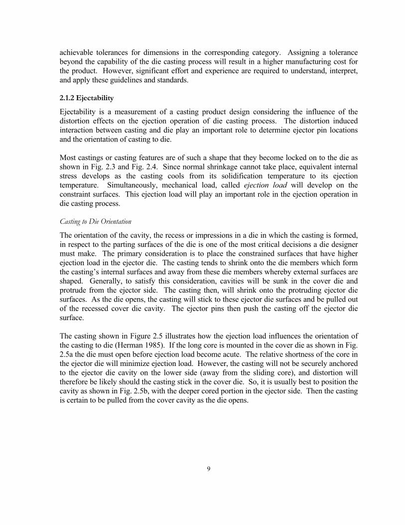
The orientation of the cavity, the recess or impressions in a die in which the casting is formed, in respect to the parting surfaces of the die is one of the most critical decisions a die designer must make. The primary consideration is to place the constrained surfaces that have higher ejection load in the ejector die. The casting tends to shrink onto the die members which form the casting’s internal surfaces and away from these die members whereby external surfaces are shaped. Generally, to satisfy this consideration, cavities will be sunk in the cover die and protrude from the ejector side. The casting then, will shrink onto the protruding ejector die surfaces. As the die opens, the casting will stick to these ejector die surfaces and be pulled out of the recessed cover die cavity. The ejector pins then push the casting off the ejector die surface.

The casting shown in Figure 2.5 illustrates how the ejection load influences the orientation of the casting to die (Herman 1985). If the long core is mounted in the cover die as shown in Fig. 2.5a the die must open before ejection load become acute. The relative shortness of the core in the ejector die will minimize ejection load. However, the casting will not be securely anchored to the ejector die cavity on the lower side (away from the sliding core), and distortion will therefore be likely should the casting stick in the cover die. So, it is usually best to position the cavity as shown in Fig. 2.5b, with the deeper cored portion in the ejector side. Then the casting is certain to be pulled from the cover cavity as the die opens.

10

Figure 2.5: An example of casting to die orientation (Herman 1996)

A mistake in the original planning of casting to die orientation will be the most difficult to correct after the die is built. Many features of a die design can be modified without great difficulty, but once the orientation of the cavity has been determined, it is hardly ever possible to make alterations without radical changes in die construction.

It is in the immediate vicinity of the cavity that the forces are concentrated, the molten metal flows, and heat is transferred to make each casting. In this same immediate region the die must open to release the solidified casting. All of these factors will influence the ejection load on the constrained surfaces. Therefore, for a given casting design, usually, there are a lot of dispositions that the die designers should consider. Efficient tools to evaluate ejection load for each disposition will be great helpful for making decision about casting to die orientation.

Ejector pins

After the casting has solidified and the die is opened, the ejector pins are moved forward to push the casting out of the ejector die half. With the help of the ejector pins, the ejection load acting on the constrained surfaces of castings will be released. The position, number and size of ejector pins must be carefully planned to overcome the resistance to ejection. The geometric characteristics and the ejection load of castings play important roles in determining the ejector pin’s number, location, size, shape, and distribution. A good ejector pin design must be established to issue a deformation free, fast, and smooth ejection operation.

11

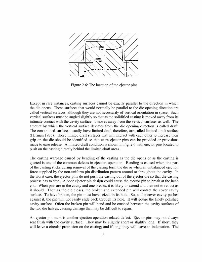
Figure 2.6: The location of the ejector pins

Except in rare instances, casting surfaces cannot be exactly parallel to the direction in which the die opens. Those surfaces that would normally be parallel to the die opening direction are called vertical surfaces, although they are not necessarily of vertical orientation in space. Such vertical surfaces must be angled slightly so that as the solidified casting is moved away from its intimate contact with the cavity surface, it moves away from the vertical surfaces as well. The amount by which the vertical surface deviates from the die opening direction is called draft. The constrained surfaces usually have limited draft therefore, are called limited draft surface (Herman 1985). Those limited draft surfaces that will interact with each other to increase their grip on the die should be identified so that extra ejector pins can be provided or provisions made to ease release. A limited-draft condition is shown in Fig. 2.6 with ejector pins located to push on the casting directly behind the limited-draft areas.

The casting warpage caused by bending of the casting as the die opens or as the casting is ejected is one of the common defects in ejection operation. Bending is caused when one part of the casting sticks during removal of the casting form the die or when an unbalanced ejection force supplied by the non-uniform pin distribution pattern around or throughout the cavity. In the worst case, the ejector pins do not push the casting out of the ejector die so that die casting process has to stop. A poor ejector pin design could cause the ejector pin to break at the head end. When pins are in the cavity and one breaks, it is likely to extend and then not to retract as it should. Then as the die closes, the broken and extended pin will contact the cover cavity surface. To have broken, the pin must have seized in its hole. So, as the cover cavity pushes against it, the pin will not easily slide back through its hole. It will gouge the finely polished cavity surface. Often the broken pin will bend and be crushed between the cavity surfaces of the two die halves, causing damage that may be difficult to repair.

An ejector pin mark is another ejection operation related defect. Ejector pins may not always seat flush with the cavity surface. They may be slightly short or slightly long. If short, they will leave a circular protrusion on the casting; and if long, they will leave an indentation. The

12

protrusion, indentation, or circular line (if the pin is flush) is called an ejector pin mark. The ejector pin mark may be raised or depressed as mush as 0.015 in. (0.4mm). The locations of the ejector pins must be limited to those areas on the casting where such marks are acceptable.

Herman (Herman 1995) has summarized a list of design guidelines to help designers and engineers choose an appropriate ejector pin location:

• Provide an ejection force directly behind all limited-draft areas. • Provide a uniform pattern of ejector pins. • Provide at least one ejector pin for each overflow. • Avoid ejector pins behind moving cores. • Avoid ejector pins in line with cover die cavity surfaces or features that are fragile or

that will form hardware quality surface finishes on the casting. Unfortunately, it is not enough to follow these rules only to establish ejector pin design because of other key factors that determine position, number, size, shape of ejector pins are not considered in these rules, such as ejection load, constrained surfaces and their interaction, die open direction. The complicated calculation of ejection load and geometric complicity of castings are necessary to get required information. Besides, identifying the limited draft surface, the constrained surfaces, in which these rules are applied individually, is not an easy task because of the complexity of castings and the interaction between the constrained surfaces.

2.2 The Factors That Influence to Casting Distortion

Die casting process is a very complex manufacturing process that involves fluid dynamics solidification, heat transfer, thermal elastic and plastic phenomena. All these physical phenomena can influence casting distortion. The governing differential equations to describe the shrinkage relative phenomena such as mechanical equilibrium equations, energy balance equations to describe transient heat conduction, entropy balance equations to describe phase change, and mass conservation and momentum balance equations to describe effect of fluid flow are fully coupled with state variables, temperature and time, and boundary constraints. In addition, as a manufacturing process, the manufacturing and technological factors, such as the interaction between casting and mold, clamping force, cycle time, and the interaction among the die components, parting line geometry, will influence to casting distortion. In the following sections, some of the factors related to the physical phenomena that have significant influence on casting distortion will be enumerated and discussed. The factors discussed are ranked from the most to the least significant influence on casting distortion.

Modeling of Dimensional Variation of Castings

The strain ε during solidification and cooling is composed of elastic, thermal and inelastic stain components:

ε = εe + εT + εp (2.1)

13

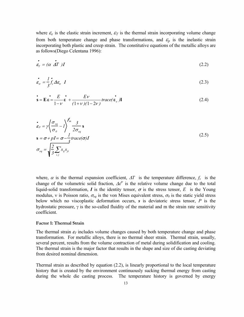
where εe is the elastic strain increment, εT is the thermal strain incorporating volume change from both temperature change and phase transformations, and εp is the inelastic strain incorporating both plastic and creep strain. The constitutive equations of the metallic alloys are as follows(Diego Celentana 1996):

εT

•= (α ∆T

• )Ι (2.2)

ε tr

•=

13

fs

•∆εtr Ι (2.3)

IεεεEs )(trace))((

EEe

••••

−++

−==

ννν

ν 2111 (2.4)

ε•

p = γσ eq

σ 0

− 11

m 32σeq

s

s = σ+ pΙ = σ−13

trace(σ)Ι

σeq =23

sij sjii, j∑

(2.5)

where, α is the thermal expansion coefficient, ∆T is the temperature difference, fs is the change of the volumetric solid fraction, ∆εtr is the relative volume change due to the total liquid-solid transformation, I is the identity tensor, σ is the stress tensor, E is the Young modulus, ν is Poisson ratio, σeq is the von Mises equivalent stress, σ0 is the static yield stress below which no viscoplastic deformation occurs, s is deviatoric stress tensor, P is the hydrostatic pressure, γ is the so-called fluidity of the material and m the strain rate sensitivity coefficient.

Factor 1: Thermal Strain

The thermal strain εT includes volume changes caused by both temperature change and phase transformation. For metallic alloys, there is no thermal sheer strain. Thermal strain, usually, several percent, results from the volume contraction of metal during solidification and cooling. The thermal strain is the major factor that results in the shape and size of die casting deviating from desired nominal dimension.

Thermal strain as described by equation (2.2), is linearly proportional to the local temperature history that is created by the environment continuously sucking thermal energy from casting during the whole die casting process. The temperature history is governed by energy

14

equations, including the effects of transient heat conduction, solidification, shrinkage-dependent interfacial heat transfer, and fluid flow(Thomas 1995).

The thermal strain is the most important “source” to generate the dimensional variation in die casting process. The stresses are generated in a casting mainly by the few percent of thermal contraction (strain) that accompany the cooling of metal in the solid state. It is important to emphasize that thermal strain does not cause stress directly. It simply creates a thermal “load” that promotes elastic strains, which cause the stress.

After ejection, castings will continue to shrink. Without restriction of the die wall, there is no interaction between castings and die wall. Therefore, there is no external stress developing on castings’ surface. Furthermore, if the castings are put in air after ejection and the castings have thin wall geometric characteristic, the effects of the internal stress caused by non-uniform mass and temperature distributions among the castings can be ignored compared with the thermal strain caused by temperature difference. Therefore, thermal strain is the dominant factor to influence the dimensional variation of castings after ejection.

Factor 2: Elastic Strain

The stress in castings arises from a number of factors. Some of these are related to the alloy itself and some are a result of the mechanical interaction between the casting and the die. But eventually, the stress is due to the thermal strain, which causes the “mismatch” as described in above. Due to the nature of die-casting, high temperature, metallic alloys, and thin wall geometric characteristic, the contribution of the elastic strain in casting to the dimensional variation is smaller than that of the thermal strain.

Elastic strain is directly responsible for stress described in equation (2.4). Stress generated in a casting is mainly caused by the few percent of thermal contraction (strain) during the cooling in solid state. Although thermal strain does not cause stress directly, it creates a “mismatch” that generates elastic strain. (Thomas 1995)

For metallic alloys, the elastic modulus E in (2.4) decreases significantly with increasing temperature. An approximate relationship between the temperature and elastic modulus is given by Zener (Zener 1948):

E = E0 [1− (

TTM

)2 ] (2.6)

where, E0 is Young’s modulus at absolute zero, and TM is melting temperature of metal.

This means that microstructural relaxation continually acts to reduce stress in a casting by replacing elastic strain with plastic strain and creep. The phenomenon is very complex, and depends on the stress and temperature histories in addition to the composition and microstructure of the material, which also evolves with time.

15

Due to the nature of die-casting, high temperature, metallic alloys, and thin wall geometric characteristic, the contribution of the elastic strain in casting is smaller than the thermal strain.

Factor 3: Inelastic stain

Inelastic strain consists of plastic strain and creep. The inelastic strain rate depends on the stress as described in equation (2.4). Relatively little data is available in the literature regarding this mechanical behavior at the high temperature, low stains, and low strain rates important to casting. For the die casting process, small strain, and small strain rate (for thin aluminum casting, the maximum value of strain rate is reported on the order of 1.0 -2 sec -1 and the maximum value of strain is in the order of 1.0-2 (Asbjorn Mo 1991)), the inelastic strain has limited contribution to the dimensional change.

Equation (2.4) gives the relationship between the viscoplastic strain rate and the deviatoric stress tensor s. It worth noting that viscoplactic flow occurs only when the von Misses equivalent stress is greater than the static yield stress. The static yield stress is a function of temperature, when temperature increases, it decreases. According to a theoretical calculation in the continuous casting process by Mo, the inelastic strain almost has the same order of magnitude of thermal strain in aluminum casting (maximum, 1%, to 2% at temperature) (Asbjorn Mo 1991). However, the inelastic strain can be negligible after the temperature of the casting drops far below solid molten temperature.

Factor 4: Interaction with Die

The interaction between the casting and the die affects the final size and shape of the casting in several different ways, creating thermal resistance and building mechanical stress. These will create the dimensional variation of castings.

First heat extraction through the die affects the temperature history of the casting. And also, the thermal resistance of the gap that forms between the solidifying shell and the die affects the heat transfer.

Secondly, the die can interact mechanically with the shell if contact occurs. Contact and friction against the die is the source of many of the stresses in a casting. The contribution of the elastic strain in casting to dimensional variation is smaller than the thermal strain. Therefore, the contribution of the interaction between die and castings is also small compared to the contribution of the thermal strain. However, the interaction will create non-uniform distortion.

Factor 5: Phase transformation

Solid-state phase transformation affects stress generation in two ways. First, it generates large volumetric expansion or contraction, which can be treated as thermal strain in equation (2.3). The volumetric change can be accounted for in the temperature-dependent density function by calculating a weighted average density based on the mass fractions of the phases present. This allows a separate microstructure model to find the phase fractions present at each time and position in the casting (G. G. Thomas 1987).

16

Secondly, phase transformation is accompanied by significant changes in mechanical properties. The atomic rearrangement during phase transformation induces inelastic stain, in proportion to the existing stress(J.B. Leblond 1986). The contribution to dimensional variation caused by mechanical property change is relative small.

Factor 6: Effect of Fluid Flow

The convective heat transfer arising from fluid flow will influence the temperature history, therefore, influence the strain and stress developing in die-casting. Unfortunately, it is extremely expensive and difficult to simulate all three phenomena (fluid flow, solidification heat conduction, and stress generation) simultaneously using a single model. No data was found from published papers.

Due to nature of die casing, filling time is very short (the order of 50ms) or less and parts are generally thin walled. One can assume that the effect of fluid convection heat transfer effect can be treated as regular solid heat transfer and could be a minor factor to influence the final shape and size of casting.

2.3 Numerical Simulation to Evaluate Casting Distortion

Mathematical modeling of stress generated in the casting processes is a subject that has received relatively less success compared to other physical phenomena that take place in die casting process (Thomas 1993). One of the reasons that stresses have received less success is that the governing phenomena are extremely complex and present a lot of computational difficulties. A mechanical “stress” model should track displacements, strains, stresses and forces as they evolve incrementally through time to fully evaluate the stresses arising during solidification and cooling (Diego Celentana 1996). The governing differential equations to describe the stress-relative phenomena such as mechanical equilibrium equations, energy balance equations to describe transient heat conduction, entropy balance equations to describe phase change, and mass conservation and momentum balance equations to describe the effect of fluid flow are fully coupled with state variables, temperature and time. The boundary conditions also are highly coupled, as temperature is dependent on the heat loss at the casting/die interface where mechanical interaction or air gap may develop. The die can interact mechanically with the shell if contact occurs. Contact and friction against the die is the source of many of the critical stresses in a casting. The nature of the die materials greatly influences the methods used for the calculation of the interaction between casting and die. Therefore, there is plenty of work still remaining for stress modeling and algorithm development for casting processes, in addition to its application to real problems (Thomas 1993).

Over the past decade, the vast majority of numerical procedures have been developed in both CV/FV(control or finite volume)(Y. D. Fryer 1993) and FE (finite element)(Michel Bellet 1993) methods to simulate the phenomena. Simulating this complex process involves solving the coupled governing equations with coupled boundary conditions. In spite of numerous simplifying assumptions, numerical modeling of the distortion still requires relatively long computation times. Despite the huge gains in computer power in recent years, the computing

17

power and ability to tackle and solve real casting stress is only beginning. Many challenges still remain before stress modeling of casting becomes a commonplace useful numerical simulation tool.

Furthermore, besides a deep understanding of thermomechanical knowledge, the use of the modeling systems requires much simulation experience and skill. For both of these reasons, existing distortion modeling approaches cannot be efficiently used for preliminary part and die design(Cross 1993).

In summary, the modeling of stress generation in casting processes is very complex and current models cannot comprehensively incorporate all of the important phenomena. Much progress has been made in all aspects. To be useful, stress models of casting processes must focus on a specific objective, make careful assumptions, and account for the most important aspects of mechanical behavior for that objective and for the particular casting process being studied. Furthermore, even assuming that casting distortion can be effectively modeled with numerical modeling schemes (e.g., FEA), numerical simulation can be hardly used in early stage of a design because too little is known about the design. An alternative approach for representing and reasoning with incomplete knowledge about casting distortion for a given design should be developed to qualitatively evaluate casting distortion.

2.4 Qualitative Reasoning Approach

Given a computerized representation of the design and a manufacturing process, manufacturing process evaluation should be able to determine what the manufacturing problems the design will generate and whether or not the design can be produced using the manufacturing process. If the design is not manufacturable, a successful manufacturing process evaluation should be capable of identifying the design attributes that pose manufacturability problems (Satyandra K. Gupta 1995).

Due to the nature of the die casting process, the part geometry is very complex and severely restricts the die design. The part design for die-casting will affect productivity, the quality of the resulting products, and therefore the production cost. Furthermore, the manufacturing concerns, such as filling, solidification, cooling and shrinkage, are volumetric phenomena that require a global consideration of the part geometry involved. However, die castings are typically designed based purely on the functional requirements and the manufacturability of the die casting usually is not considered until the design is nearly completed, or even worse, until die design is started. In this stage any modification of the design will remarkably increase both time and cost of the product development. Therefore, early diagnosis of manufacturability is essential for decreasing costs of both development and production.

Numerical modeling schemes and qualitative approach are two important techniques to evaluate the manufacturability for a given design. Numerical simulations are based on numerical analysis techniques such as finite element, finite difference and boundary element engineering analysis tools. These provide differential equation solutions to obtain the predicted physical fields, the thermal shrinkage in our case, distributed throughout the space occupied by

18

the part. The data generated from numerical methods is based on not only the design information but also material data and process information, such as initial temperature of die and the casting ejection temperature, die cooling etc.

In contrast, qualitative reasoning is a method for representing and reasoning about physical mechanism with incomplete knowledge. Geometric reasoning approach to qualitatively evaluate a given design can be described as (Kuipers 1994), for a given model representing the incomplete knowledge available at the current state of the design process, to predict the behaviors of the model consistent with known geometric representation of the design. The predictions will be checked against the specifications for the product being designed. If some behaviors violate the specifications, the geometric entities that create the violation will be reported and modification of the geometric entities will be suggested to prevent those behaviors. The predictions could be used to create additional specifications that will help the design or manufacturing of the product. A qualitative description is one that captures distinctions that make an important, qualitative difference, and ignores others. Undoubtedly, the ability to focus on the important distinctions and ignore the unimportant ones is an excellent way to cope with incomplete knowledge.

In the case of casting distortion evaluation, for a given casting design, some design characteristics could induce constrained shrink, such as any design involving a channel or I-beam section with Tee junctions, that can lead to a situation in which the die wall resists normal contraction (George W. Anselman 1974). As described in previous section, the design characteristics will influence the dimensional variation, ejectability, and casting to die orientation. On the other hand, other characteristics may cause free shrink that generates the relatively large dimensional variation of the casting and develops air gaps between the casting and die wall that may create heat transfer problems.

2.4.1 Early Manufacturability Evaluation

If manufacturing incompatibility of a product can be evaluated at the early product design stage, the designers can modify their design to reduce the effect of the manufacturing problem. This will result in fewer manufacturing problems. Less redesign, less expensive tooling, lower cost, better quality, and shorter development time. This is the concept of design for manufacturing (DFM) (Ishii 1995).

“A numerical simulation is useless in the early stages of design because too little is known” (Forbus 1988). Although the comment cannot be completely accepted, it is quite true from a certain point of view. The thermal strain data generated from numerical methods is based on not only the design information but also material data, process information, boundary conditions. For example, to determine the thermal strain, the temperature history has to be determined; and to determine temperature history, heat transfer boundary conditions, heat transfer coefficients, thermal expanding coefficient, initial temperature of die and the casting eject temperature, etc. should be determined before the simulation begins. The information usually is not available in the early stage of a casting design.

19

In contrast, by performing geometric reasoning, it is possible to extract potential manufacturing problems of a product design based on the geometric and topologic information of the design. Also, it is possible to extract these design characteristics that have significant influence on manufacturability. These can give casting designers diecastability feedback about their design and help them to make design decisions to reduce the effects of casting distortion.

2.4.2 Interpretation of the Evaluation Results

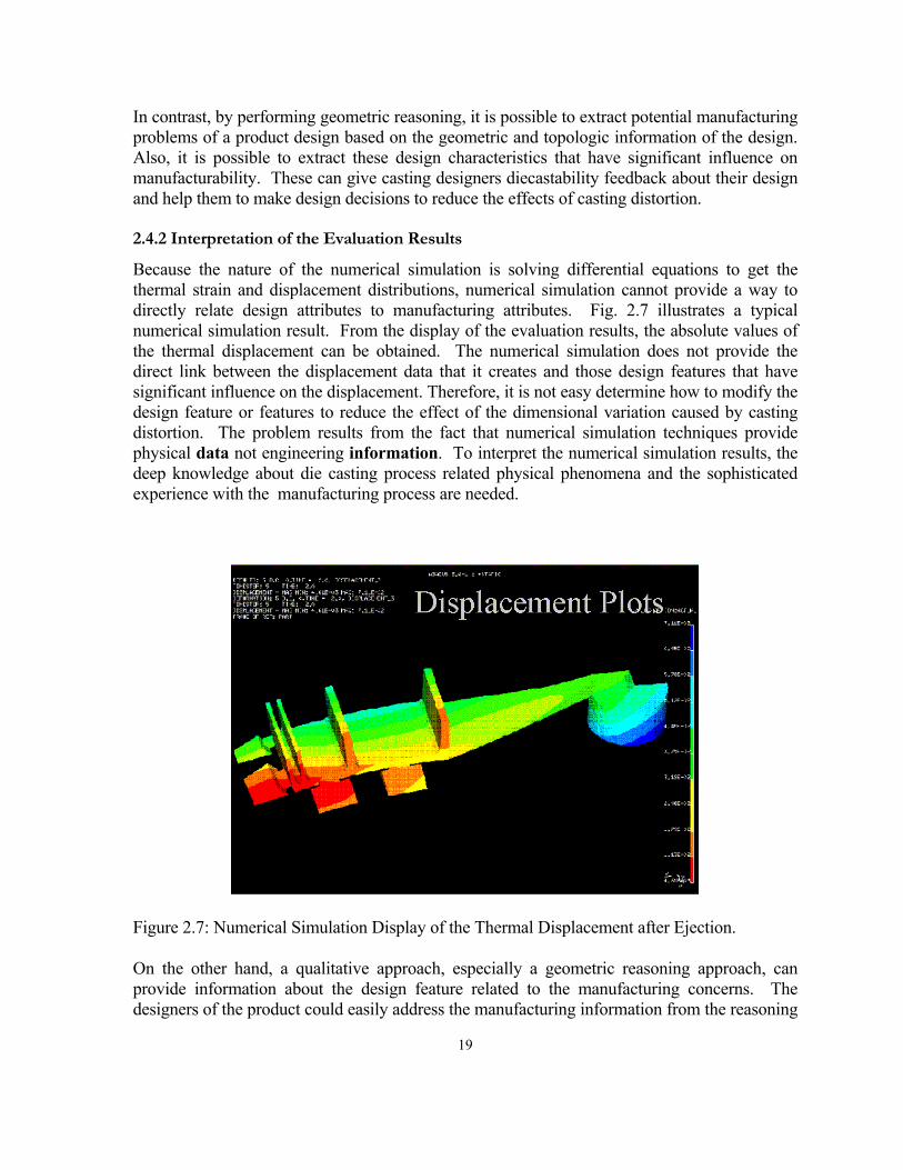
Because the nature of the numerical simulation is solving differential equations to get the thermal strain and displacement distributions, numerical simulation cannot provide a way to directly relate design attributes to manufacturing attributes. Fig. 2.7 illustrates a typical numerical simulation result. From the display of the evaluation results, the absolute values of the thermal displacement can be obtained. The numerical simulation does not provide the direct link between the displacement data that it creates and those design features that have significant influence on the displacement. Therefore, it is not easy determine how to modify the design feature or features to reduce the effect of the dimensional variation caused by casting distortion. The problem results from the fact that numerical simulation techniques provide physical data not engineering information. To interpret the numerical simulation results, the deep knowledge about die casting process related physical phenomena and the sophisticated experience with the manufacturing process are needed.

Figure 2.7: Numerical Simulation Display of the Thermal Displacement after Ejection.

On the other hand, a qualitative approach, especially a geometric reasoning approach, can provide information about the design feature related to the manufacturing concerns. The designers of the product could easily address the manufacturing information from the reasoning

20

results and modify their designs to reduce manufacturing problems. The geometric reasoning approach directly applies the model representing the incomplete knowledge available at the current state of the design process to the elementary entities of the part representation to extract the design characteristics that could induce the manufacturing problem.

2.4.3 Simple to use

Even if we assume that the numerical techniques can effectively model the casting distortion, the essential steps to run the numerical simulation such as meshing in FEA, setting up boundary conditions, require deep knowledge about the die casting related physical phenomena and experience with numerical simulation. These create a great difficulty for the designers of casings who possibly have little or no knowledge and experience to run the numerical simulations.

Qualitative approaches, like geometric reasoning, usually are easy to use compared to the numerical simulation. For geometric reasoning, the only input data to perform the evaluation is the geometric representation of the parts. There are no boundary conditions and die casting process data required. No specific simulation techniques such as meshing are required.

2.4.4 High Efficiency

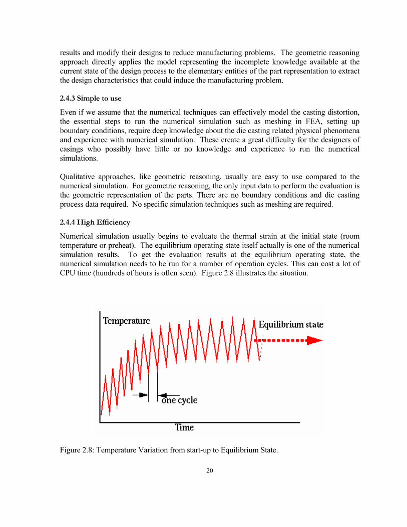
Numerical simulation usually begins to evaluate the thermal strain at the initial state (room temperature or preheat). The equilibrium operating state itself actually is one of the numerical simulation results. To get the evaluation results at the equilibrium operating state, the numerical simulation needs to be run for a number of operation cycles. This can cost a lot of CPU time (hundreds of hours is often seen). Figure 2.8 illustrates the situation.

Figure 2.8: Temperature Variation from start-up to Equilibrium State.

21

In contrast to the numerical simulation, geometric reasoning could make evaluation at the equilibrium state. This makes the geometric reasoning much more efficient than the numerical simulation.

2.5 Complementary of numerical simulation and qualitative approach

Both qualitative approach and numerical simulation can promote the compatibility between a given design and the die casting process. However, as discussed above, the two approaches have their own characteristics. Numerical simulations can provide quantitative, detail, and accurate, systematic, and time resolved manufacturing data for a given design. Moreover, numerical simulation can be used to evaluate the design of a manufacturing process for a given part design to obtain or modify process parameters. So, with these with characteristics, numerical simulations cannot be replaced by qualitative approaches. Therefore, the complementary characteristics of the two approaches are not only important but also practical.

2.5.1 Performing Quantitative Approach and Numerical Simulation at Different Periods of

Product Development

If we examine the spectrum of design evaluation tools along the product development timeline in die casting as illustrated in Figure 2.9, they fall into two main periods, earlier design stage and the late design stage.

As mentioned above, one of advantages of the qualitative approach is the support of DFM. It facilitates evaluation during the early stages of design development. Using qualitative approach techniques, the designers can modify their designs to reduce the incompatibility with die casting process. In other word, qualitative approach can be easier used to support design decision-making.

Design Tooling

Numerical Simulation

(more accurate, timeconsuming, requiresmuch skill, used forchecking and post-design verification)

Geometry-Driven Analysis(less accurate, quick,

easy to use, easy to interpret)

Figure 2.9: Die Casting Development Timeline Showing Spectrum of Design Evaluation Techniques(Rebello 1997).

22

After the design is nearly completed, numerical simulation can be used to check the incompatibility of the detail design features and to help to decide and check the die casting process parameters for the design.

2.5.2 Performing Quantitative Evaluation before Numerical Simulation

A qualitative evaluation can serve as a pilot evaluation before performing numerical simulation because of qualitative evaluation’s efficiency. The qualitative results could help to speed convergence of the numerical iteration. The qualitative approach can help to set up boundary conditions in the evaluation of thermal strain by numerical simulation. As discussed in the previous section, coupling of the thermal and mechanical boundary conditions will create difficulty for numerical simulation to evaluate the casting distortion. The thermal resistance of the gap that forms between the solidifying shell and the die affects the heat transfer. To get temperature history, a suitable heat transfer boundary condition is necessary. If the qualitative approach could provide where the gap will form, we can get a good start to set up the boundary condition. On the other hand, condition if the constrained surfaces can be determined by the approach, this could also help to setup mechanical boundary.

To get the equilibrium temperature in die casting, numerical simulation usually need to be run a great number (say 100) die casting cycles. If qualitative reasoning can provide a relative initial temperature distribution, like the thick section data (Lu 1996), the number of the start up iteration of numerical simulation could be greatly reduced.

2.5.3 Performing Quantitative Evaluation and Numerical Simultaneously

As mentioned before, to interpret the numerical simulation, deep knowledge about the die casting process and related physical phenomena is required. The qualitative approach can provide easily understandable dimensional variation information. If the qualitative and numerical simulation could be run simultaneously, it will help to interpret the simulation results. Moreover, the results of qualitative evaluation and numerical simulation could be used to check each other to verify the consistency of the results

23

3. QUALITATIVE REASONING OF CASTING DISTORTION

3.1 Introduction

The evaluation of the casting thermal distortion is involved in the thermal stress-strain analysis. The modeling of stress-strain generation in casting processes is very complex and current models cannot comprehensively incorporate all of the important phenomena. To be useful, stress models of casting processes must focus on a specific objective, make careful assumptions, and account for most important aspects of mechanical behavior for that objective and for the particular casting process being studied.

In this chapter, qualitative methods are introduced for evaluating the temperature distribution of castings, free shrinkage, and constrained distortion. The heat conduction taking place in the cooling process of castings, the free shrinkage and the constrained distortion of castings have been reduced to the Poisson’s equation forms. The spatial casting temperature, the displacements of free shrinkage and constrained distortion are expressed as functions of the distance to the equivalent source entities by means of one of the important particular solution of Poisson’s equation, volume potential. The geometric reasoning methods discussed in next chapter will utilize distance transforms for evaluating the distance-related functions based on the geometric and topologic information of given castings.

Geometry-driven analyses will concentrate on what part geometry can result in thermal distortion related problems. To emphasis the effects caused by the part geometry, the steady state is assumed when performing the qualitative evaluation. Analyzing at steady state also means that the effects that result from the transient behaviors will be ignored. For example, neglecting the time dependent term in heat conduction equation means that the time-rate related inertia has been ignored.

3.2 Laplace’s Equation and Volume Potential Theory

In a study of a variety of steady state problems, elliptic type differential equations often arise (Tikhonov, 1990). The most common equation of this type is Laplace’s equation

02 =∇ u (3.1)

The function u is said to be harmonic in the domain Ω, if it is continuous in this region together with its derivatives up to second order and if it satisfies Laplace’s Equation. ∇2 is the Laplacian operator that, under Cartesian coordinates, can be represented as:

24

2

2

2

2

2

2

zyx ∂∂

+∂∂

+∂∂

Laplace’s equation is the most common elliptic type differential equation and governs many physical processes in steady state. As discussed later in this section, casting thermal distortion related physical processes in steady state, such as heat conduction, and displacement of thermal elastic distortion, can be reduced to the Laplace’s equation. The inhomogeneous version of Laplace’s equation is called Poisson’s equation:

)z,y,x(fu =∇ 2 (3.2)

Assume that M, and M0 are two points in the region Ω, the solution U(M,M0) that satisfies equation,

=∞≠

=−=∇

0

0

00

2

MM,MM,

)MM(u δ (3.3)

is called the fundamental solution of Poisson’s equation

fu =∇ 2 (x,y,z)

where δ(M,M0) is δ-function. Sometimes, the solution is also referred to as the fundamental solution of Laplace’s equation 02 =∇ u (Tikhonov, 1963).

The fundamental solution of Poisson’s equation satisfies:

002 when0 MM)M,M(u ≠=∇ (3.4)

for a smooth source function f(M),

000 dM)M(f)M,M(U)M(U ∫Ω

= (3.5)

The fundamental solutions have different representations in 2-dimensional and 3-dimensional rectangle coordinate systems (Tikhonov, 1963):

2-dimension: 0

121

0M,Mr

ln)M,M(Uπ

= (3.6)

3-dimension: 0

141

0M,Mr

)M,M(Uπ

= (3.7)

25

n-dimension: 3n 1

22

22

20

0

>−

Γ= −n

M,Mn r

)n(

)n()M,M(U

π (3.8)

where 0M,Mr is the distance between M and M0.

The fundamental solutions, U(M,M0), of Laplace’s equations are one of the particular solutions of the Laplace’s equations. They are the solution for a unit point source of Poisson’s equations satisfying so-called natural boundary conditions. The boundary-value problem of the particular solution can be written as:

∞=

=

=∞≠

=−=∇

→

∞→−

0

00

0

0

000

2

MM

MM

u

u

MM,MM,

)MM()M,M(U δ

(3.9)

3.2.1 Potential Theory

The volume potential has an intrinsic value from the point of view of direct application in physics, such as gravity potential field, temperature field, elastic displacement potential field, and static electrical potential field etc. In addition, a potential function provides another method for solving boundary-value problems.

The foundation of the potential theory is the fundamental solution of Laplace’s equation U(M,M0) and the superposition of the fundamental solutions. The function

2

12220

11

])z()y()x[(r)M,M(U

ςηξ −+−+−== (3.10)

representing the potential of a unit source situated at point M0(ξ,,η, ζ) is a solution of Laplace’s equation, depending on the parameters ξ,η,ζ. The integral of this function over these parameters Eq.3.10 is called potential function that is the fundamental solutions of the Poisson’s equation with source function f(x,y,z) defined in region Ω. In 3-dimensional case, it is called as volume potential:

τdr

)z,y,x(f)M(u ∫Ω

=1 (3.11)

The volume potential is a direct result of superposition of the fundamental solution of Poisson’s equations. The potential function of n point sources is expressed by the relation:

26

∑ ∑= =

==n

i

n

i i

ii r

fuu1 1

(3.12)

Based on the potential function, a vector field F, sometimes called the flux vector of potential u, can be defined so that (Tikhonov, 1963):

u∇=F (3.13)

where ∇ is the gradient operator and the projections of this vector on the coordinate axes are:

−−=

∂∂

=

−−=

∂∂

=

−−=

∂∂

=

∫

∫

∫

Ω

Ω

Ω

τς

τη

τξ

dr

zfzuZ

dr

yfyuY

dr

xfxuX

3

3

3

(3.14)

3.2.2 Asymptotic Expression for the Volume Potential

In an investigation of the volume potential

MPT

P rdd

d)P()M(V == ∫∫∫ where

τρ (3.15)

at great distances from the distributed source T and with the source intensity ρ, it is usually assumed that the potential equal to m/R, where m is the total intensity of the distributed source T, R is the distance of its center from the point of observation. A more exact asymptotic expression for V can be determined by the following discussion.

Let Σ be a sphere with center at the origin entirely containing the body T. Outside this sphere the potential will be a harmonic function.

27

TO

Mi

M

d

rri θ

TO

Mi

M

d

rri θ

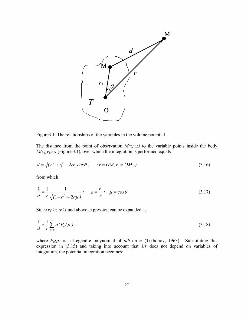
Figure3.1: The relationships of the variables in the volume potential

The distance from the point of observation M(x,y,z) to the variable points inside the body M(x1,y1,z1) (Figure 3.1), over which the integration is performed equals

)OMr,OMr()cosrrrr(d 1112

12 2 ==−+= θ (3.16)

from which

θµµ

cos;rr

a;)aa(rd

==−+

= 21

111 1

2 (3.17)

Since r1<r, a<1 and above expression can be expanded as:

∑∞

=

=0

11n

nn )(Pa

rdµ (3.18)

where Pn(µ) is a Legendre polynomial of nth order (Tikhonov, 1963). Substituting this expression in (3.15) and taking into account that 1/r does not depend on variables of integration, the potential integration becomes:

28

...d)(Prr

d)(Prr

dr

...VVVd)(Par

)M(V

TTT

T nn

n

+++=

=+++==

∫∫∫∫∫∫∫∫∫

∫∫∫ ∑∞

=

τµρτµρτρ

τµρ

22

13112

320

1

1 11

1

(3.19)

The first term equals m/r where m is the total source intensity of the distributed source, and gives a first approximation of the calculation of the potential for large r.

The expression under the integral sign in the second term is

rzzyyxxrr)(P 111

111 ++== ρµρµρ (3.20)

The values x,y,z and r do not depend on the variables of integration and may be taken outside the integral sign. Thus the second term of the expansion of the potential takes form (Tikhonov, 1963):

)zzyyxx(r

M)zMyMxM(r

d)(Prr T

++=++=∫∫∫ 3113112

1 1 τµρ (3.21)

where

∫∫∫

∫∫∫∫∫∫==

====

T

TT

zMdzM

yMdyMxMdxM

τρ

τρτρ

13

1211

, , (3.22)

are moments of first order, z,y,x are the coordinates of the center of gravity if the ρ expresses the density and V(M) is the potential of the gravity. Thus, the second term decreases as 1/r2. If the origin of the coordinate system is located at the center of gravity ( 000 === z,y,x ), then V2 = 0. It can be shown that the third term of the expansion will decrease as 1/r5, and therefore can be ignored comparing the first term (Tikhonov, 1963).

Consequently, the asymptotic expression for the potential can be arrived:

)zzyyxx(rm

rmV +++≅ 3 (3.23)

which is valid up to terms of order 1/r5. Expression (3.23) is simplified if the origin of coordinates at the center of gravity:

29

rmV ≅ (3.24)

where, r is the distance between the gravity center and observation point. If the distributed source has the same source intensity, r is the distance between the geometric center of the source and the observation points. Expression (3.24) means that the potential of a distributed source at a large distance from it can be approximated as the potential of a point source at the same point. The point source locates at the gravity center of the distributed source and with the source intensity of the total source intensity of the distributed source.

For the qualitative reasoning of casting distortion, the distributed source T will be digitized as a collection of identical cubic units (this process is called voxelization and will be discussed in the next chapter, Geometric Reasoning of Casting Distortion). The digitized source can be categorized as groups ti according to their source intensity ρi so that each group has the same source intensity. According to the linear superposition theory, the potential can be expressed as:

∑=

=N

i i

i

rm)M(V

0 (3.25)

where, ri is the distance between the ith geometric center and M, mi is the total intensity of the ith group.

3.3 Volume Potential and Body Force Analogy of Thermoelastic Problems

The theory of elasticity aims to investigate the deformations arising in elastic bodies by mathematical methods. Strain originating from the action of external forces can be characterized by means of a displacement vector u at every point, whose projection on the coordinate axes x, y, z are denoted by u(x,y,z,t), v(x,y,z,t), and w(x,y,z,t). These displacements arise in an elastic body under the action of internal forces (stress), which form a symmetrical stress tensor.

zzyzx

yzyyx

xzxyx

στττστττσ

where, σx, τxy, τxz are the components of force (stress), acting on unit area of a surface element, perpendicular to the x-axis; similarly, τyx, σy τyz and τzx, τzy σz, are the components of stresses, acting on unit area of surface elements, perpendicular to the x, and axes. The components σy,

σx,, σx are called normal stresses, and τxy, τxy etc. are called the shear stresses. Considering an element of volume, its motion equation can be written as (Tikhonov, 1963):

30

+∂∂

+∂

∂+

∂∂

=∂∂

+∂

∂+

∂

∂+

∂

∂=

∂∂

+∂∂

+∂

∂+

∂∂

=∂∂

Zxzyt

w

Yzxyt

v

Xzyxt

u

zzyzx

yzyyx

xzxyx

σττρ

τστρ

ττσρ

2

2

2

2

2

2

(3.26)

where ρ is the volume density at the point (x,y,z), X, Y, Z are the components of the external volume forces. The values of stresses, arising from strains, are given by Hooke’s law, which is written in the following form:

=

−+=

=

−+=

=

−+=

zxxyzz

yzyzyy

xyxyxx

G,m

G

G,m

G

G,m

G

γτθεσ

γτθεσ

γτθεσ

2

2

2

2

2

2

(3.27)

In Eq.3.27 the following symbols were used: G the shear modulus, m the inverse of Poisson

ratio, θ = ∇• u = zw

yv

xu

∂∂

+∂∂

+∂∂ .

The quantities

∂∂

+∂∂

=∂∂

+∂∂

=∂∂

+∂∂

=

∂∂

=∂∂

=∂∂

=

zu

xw,

yw

zv,

xv

yu

zw,

yv,

xu

zxyzxy

zyx

γγγ

εεε

(3.28)

form a symmetrical tensor of the strains

=

zzyzx

yzyyz

xzxyx

εγγγεγγγε

ε

Boundary conditions should be added to Eq.3.26 and Eq.3.27 (at the boundary, for example, displacement u, v, w, or surface force, etc. are given), which are not considered here.

Equation Eq.3.26 and Eq.3.27 form a complete system of differential equations for the stresses and strains. Substituting the expressions for the stresses from Eq.3.27 in the equation of

31

motion Eq.3.26) and taking into account relation Eq.3.28, a set of equations of the displacements can be obtained:

+∂∂

−+∇=

∂∂

+∂∂

−+∇=

∂∂

+∂∂

−+∇=

∂∂

Z)zm

mw(Gtw

Y)ym

mv(Gtv

X)xm

mu(Gtu

θρ

θρ

θρ

2

2

2

22

2

22

2

22

2

(3.29)

The constants λ and µ were introduce in place of the constant G and m, connected by the relations:

Gm

,G2

2 −

== λµ (3.30)

The preceding set of equations can be written in the form of a single vector equation (Tikhonov, 1963)

Fuuu+×∇×∇−•∇∇+=

∂∂ µµλρ )()(

t22

2

(3.31)

where u is a displacement vector with components u, v, w, F is a vector of the volume forces with components X, Y, Z.

If the external volume force F can be written as the gradient of a scalar U:

U∇=F (3.32)

The displacement u can be expressed as the gradient of scalar field, displacement potential field Φ(M), and Φ satisfies:

U)(t

+Φ∇+=∂Φ∂

Φ∇=

22

2

2µλρ

u (3.33)

If a steady state is assumed to exist, Φ satisfies Poisson’s equation:

U)( µλ 2

12

+−=Φ∇ (3.34)

32

3.3.1 Thermal stress analysis and body force analogy

Most substances expand when their temperature rises and contract when cooled, and for a wide range of temperatures, this expansion or contraction is proportional to the temperature change. This proportionality is expressed by the coefficient of linear thermal expansion (α) that is defined as the change in length that a bar of unit length undergoes when its temperature is changed by 1°.

If free expansion or contraction of all the fibers of a body is permitted, no stress is caused by the change in temperature. However, when the temperature distribution in a homogeneous body is not uniform, different elements of the body trend to expand by different amounts and the requirement that the body remain continuous conflicts with the requirement that each element expand by an amount proportional to the local temperature rise. Thus, the various elements exert upon each other a restraining action resulting in continuous unique displacements at every point. The system of strains produced by this restraining action cancels out all, or part of, the free thermal expansions at every point to ensure continuity of displacement. This system of strains must be accompanied by a corresponding system of self-equilibrating stresses. These stresses are known as thermal stress.

For thermal distortion, the total strains at each point in a heated or cooled body may be considered to consist of two parts, the free thermal expansion/contraction, thermal strain εT, plus the strains dependent on the stress, ε0, that are described in Eq. 3.28.

Tεεε += 0 (3.35)

=

TT

TT

αα

αε

000000

(3.36)

Since the thermal strain is uniform in all directions at a given point in an isotropic body, it can be deduced that no shear strains result –only direct stains.

3.3.2 Body Force Analogy

Thermal distortion can be analogized as the consequence of the action of the thermal equivalent body force fT(x,y,z) surface force qT (x,y,z) (Johns 1965):

nq 21

TET

να−

−= (3.37)

21

TET ∇−

=ναf (3.38)

33

where, ∇ is the gradient operator, n is the surface normal vector, T is the temperature distribution, and E is the Young modulus, ν is Poisson ratio, and α is the coefficient of the thermal expansion. The thermal effects caused by the temperature change, such as thermal shrinkage, strain, and stress, result from the thermal equivalent body force and surface force. The surface force is at the inverse direction of the surface normal and proportional to the temperature value. The body force is proportional to the local temperature gradient, and, therefore, sensitive to the temperature distribution. Therefore, even with the uniform temperature distribution, the casting is still under the action of the surface force.

The body force analogy may be stated as follows: the displacements and strains in a heated/cooled body will be the same as those in an unheated body of the same shape and material, if the unheated body is subjected to the equivalent body force qT and to the equivalent surface tractions fT over that portion of the boundary where surface tractions are specified, and furthermore has the same displacement conditions over that portion of the boundary where displacements are specified.

Therefore, the elastic equation Eq. 3.30 is extended to thermoelastic case:

Fuuu+

−∇

−×∇×∇−•∇∇+=∂∂

)(TE)()(

t ναµµλρ

2122

2

In steady state, the elastic equation can be written as:

Fuu −−∇

=×∇×∇−•∇∇+)(

TE)()(ν

αµµλ21

2 (3.39)

If there is no external volume force, the displacement potential satisfies:

T)()( α

νν

−+

=Φ∇

Φ∇=

112

u (3.40)

Of course, this analogy does not, in any sense, reduce the mathematical difficulties of the thermoelastic problem. In fact, the mathematical formulation of the problem of the problem is completely unchanged; all that has been done is to rename some of the given functions. However, the analogy is valuable from a conceptual viewpoint since it allows an alternative visualization of the effects of a non-uniform temperature distribution in terms of the effects of an equivalent body force system.

Although the “body force analogy” in no way reduces the mathematical complexity of a given problem, it may help to provide a clear physical interpretation of a given thermal shrinkage problem, here in our case, the casting free shrinkage.

34

3.3.3 Potential Theory to Solve Thermoelastic Boundary-value Problems

The boundary-value problem of the thermoelastic problem during the die casting process can be modeled as: for some volume Ω, bounded by the surface Σ, find the function u(M) in Ω that satisfies:

Σ∈=•+Σ∈=

−∇

=×∇×∇−•∇∇+

2

1

on 23- on

212

B(M))T)((B)M(

)(TE)()(

HnIσGu

uu

µλ

ναµµλ

(3.41)

where σ is the stress tensor and n is the normal of the boundary Σ and the G(M) and H(M) are describing vector functions. The first boundary condition is called the displacement boundary condition that regulates the displacement on the boundary B1. The second boundary condition is called a traction boundary condition that regulates the thermal stress on the boundary B2. In practice, it is possible that neither of the above sets of conditions would apply independently over the entire surface of the body and mixed boundary conditions are then involved. The displacement boundary condition can be used to describe the constrained distortion. If the die wall is assumed to be rigid, displacement is zero on the constrained surface B1 therefore, G(M) equals to 0 on B1. For the free shrinkage surface B2 where the casting can freely shrink, traction boundary can be applied so that all stress components on the normal direction of B2 are zeroes, therefore H(M)=0 on B2.

The displacement equations are a set of linear, nonhomogeneous differential equations for the unknown displacements u with the gradients of the given temperature distribution as nonhomogeneous terms. The displacements may therefore be expressed as the sum of two functions,

cp uuu += (3.42)

where the particular solutions up are any functions which satisfy the nonhomogeneous equations without regard to the given boundary conditions. Let the value which up assumes on the boundary be denoted by Gi

(p) and the surface tractions to which they correspond (though the thermoelastic stress-strain relations and the given temperature distribution) be denoted by Hp(p), that is,

Σ∈=•+

Σ∈=

2p

1

on 23-

on

B(M))T)((

B)M(p

pp

HnIσ

Gu

µλ (3.43)

Then uc must satisfy the homogeneous equations and boundary conditions:

35

Σ∈−=•+

Σ∈=

=×∇×∇−•∇∇+

2

1

on 23-

on - 02

B(M)(M))T)((

B)M()M()()(

pc

pc

cc

HHnIσ

GGuuu

µλ

µµλ

(3.44)

Under these condition, u = up + uc is a solution of the stated thermoelastic problem Eq.3.41. It is furthermore seen that the problem for the determination of uc corresponds to a constant temperature with no body forces, so that the desired reduction is accomplished as soon as a particular solution to Eq.3.41 is found.

Based on the displacement potential and body force analogy discussed in previous sections, the displacement up may all be expressed in term of a displacement potential function Φ(M) that satisfies Poisson’s equation Eq.3.34:

T)()(

p

ανν

−+

=Φ∇

Φ∇=

112

u (3.45)

From the potential theory, one solution of the above equation is the fundamental solution of Poison’s equation and can be written directly in the form of volume potential:

∫∫∫Ω −+−+−−

+=Φ

222141

)z()y()x(ddd),,(T

)()(

ςηξςηξςηξ

νπαν (3.46)

or in a more compact form, as

∫∫∫Ω−

+=Φ

)M,M(rdV)M(T

)()()M( M

0

0 0

141

νπαν (3.47)

where, r(M,M0) is the distance from the point M to the point M0.

In theory, therefore, this particular solution, for Φ provides a direct means for the reduction of every thermoelastic problem to a constant temperature problem without body forces. Unfortunately, the volume integral required by Eq.3.47 is quite difficult.

From potential theory, the volume potential, the thermoelastic displacements may be considered as the result of the distribution of centers of dilation of strength

00141

MdV)M(T)(

)(νπαν

−+ (3.48)

36

throughout the body. Therefore, if the solution for a center of dilatation in a given body free of surface tractions is known, the solution to a thermoelastic problem for that body with zero surface tractions can be obtained immediately by means of a volume integral. There are two practical difficulties with this procedure, solutions for the center of dilation are known for very few geometries with specific temperature distributions, and the multiple integral required is difficult to perform. However, the center of dilatation resulting from the temperature distributions can be obtained by analyzing the thermal equivalent body force, which is another formulation of thermoelastic problem discussed in previous section. Actually, the qualitative reasoning of the thermal distortion of castings, reported in this report, is based on the combination of these two alternative formulations of thermoelastic problems.

3.3.4 Saint Venant’s Principle

In many thermoelastic problems, some simplification is possible by using St. Venant’s principle. St. Venant’s principle states that the difference in stresses produced by two sets of statically equivalent forces acting on a surface area A diminishes with distance from A and becomes negligible at distances large compared to the linear dimensions of A.

St. Venant’s principle provides a qualitative way to estimate the effect of the statically equivalent surface forces. Especially, when thermal shrinkage problem is analogized to the force and its effect, St. Venant’s principle can help our qualitative reasoning to evaluate the free shrinkage. Additionally, when the displacement boundary condition is transferred to its equivalent force boundary, as will be shown in the constrained shrinkage section of this proposal, St. Venant’s principle can help to estimate the effect of the boundary force.

The boundary forces developed on the casting surface are statically equivalent surface forces because, under the action of the boundary forces, castings have no macroscopic movement before and after ejection. According to St. Venant’s principle, the effect of the boundary forces diminishes with the distance to the boundary. Distance transformation can be employed to calculate the voxel-based distance to the boundary. The effect of the boundary forces therefore is inversely proportional to the distance. The applications of the St. Venant’s principle will be discussed later in this report.

3.4 Temperature Reasoning

In this section, the qualitative evaluation of the casting’s temperature distribution at ejection from die is discussed. The formulation of the mathematical boundary-value problem for the determination of the temperature distribution is discussed. Since solid, opaque castings are of primary interest here, heat is transferred form point to point within the body solely by conduction. The equation of the boundary-value problem will, therefore, always be some form of the Fourier heat conduction equation. However, this mathematical model is too complex to be used in qualitative reasoning of the temperature of castings. The simplifications heat transfer model, the correlation between heat content in a casting and the wall thickness of the casting, and the correlation between the heat trap in die and the thin die area, are introduced in this section. Based on that, the temperature of castings can be qualitatively evaluated.

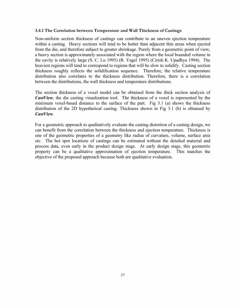
37

3.4.1 The Correlation between Temperature and Wall Thickness of Castings

Non-uniform section thickness of castings can contribute to an uneven ejection temperature within a casting. Heavy sections will tend to be hotter than adjacent thin areas when ejected from the die, and therefore subject to greater shrinkage. Purely from a geometric point of view, a heavy section is approximately associated with the region where the local bounded volume in the cavity is relatively large (S. C. Lu 1995) (R. Yagel 1995) (Cirish K. Upadhya 1994). The heaviest regions will tend to correspond to regions that will be slow to solidify. Casting section thickness roughly reflects the solidification sequence. Therefore, the relative temperature distribution also correlates to the thickness distribution. Therefore, there is a correlation between the distributions, the wall thickness and temperature distributions.

The section thickness of a voxel model can be obtained from the thick section analysis of CastView, the die casting visualization tool. The thickness of a voxel is represented by the minimum voxel-based distance to the surface of the part. Fig 3.1 (a) shows the thickness distribution of the 2D hypothetical casting. Thickness shown in Fig 3.1 (b) is obtained by CastView.

For a geometric approach to qualitatively evaluate the casting distortion of a casting design, we can benefit from the correlation between the thickness and ejection temperature. Thickness is one of the geometric properties of a geometry like radius of curvature, volume, surface area etc. The hot spot locations of castings can be estimated without the detailed material and process data, even early in the product design stage. At early design stage, this geometric property can be a qualitative approximation of ejection temperature. This matches the objective of the proposed approach because both are qualitative evaluation.

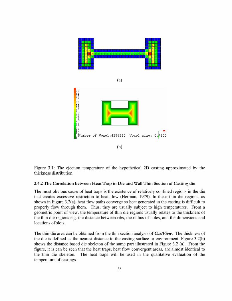
38

1 1 1 1 1 1 1 1 1 11 2 2 2 1 1 2 2 2 11 2 3 2 1 1 2 3 2 11 2 3 2 1 1 2 3 2 11 2 3 3 2 1 1 1 1 1 1 1 1 1 1 1 1 1 1 1 1 1 2 3 3 2 11 2 3 4 3 2 2 2 2 2 2 2 2 2 2 2 2 2 2 2 2 2 3 4 3 2 11 2 3 3 2 1 1 1 1 1 1 1 1 1 1 1 1 1 1 1 1 1 2 3 3 2 11 2 3 2 1 1 2 3 2 11 2 3 2 1 1 2 3 2 11 2 2 2 1 1 2 2 2 11 1 1 1 1 1 1 1 1 1

(a)

(b)

Figure 3.1: The ejection temperature of the hypothetical 2D casting approximated by the thickness distribution

3.4.2 The Correlation between Heat Trap in Die and Wall Thin Section of Casting die

The most obvious cause of heat traps is the existence of relatively confined regions in the die that creates excessive restriction to heat flow (Herman, 1979). In these thin die regions, as shown in Figure 3.2(a), heat flow paths converge so heat generated in the casting is difficult to properly flow through them. Thus, they are usually subject to high temperatures. From a geometric point of view, the temperature of thin die regions usually relates to the thickness of the thin die regions e.g. the distance between ribs, the radius of holes, and the dimensions and locations of slots.

The thin die area can be obtained from the thin section analysis of CastView. The thickness of the die is defined as the nearest distance to the casting surface or environment. Figure 3.2(b) shows the distance based die skeleton of the same part illustrated in Figure 3.2 (a). From the figure, it is can be seen that the heat traps, heat flow convergent areas, are almost identical to the thin die skeleton. The heat traps will be used in the qualitative evaluation of the temperature of castings.

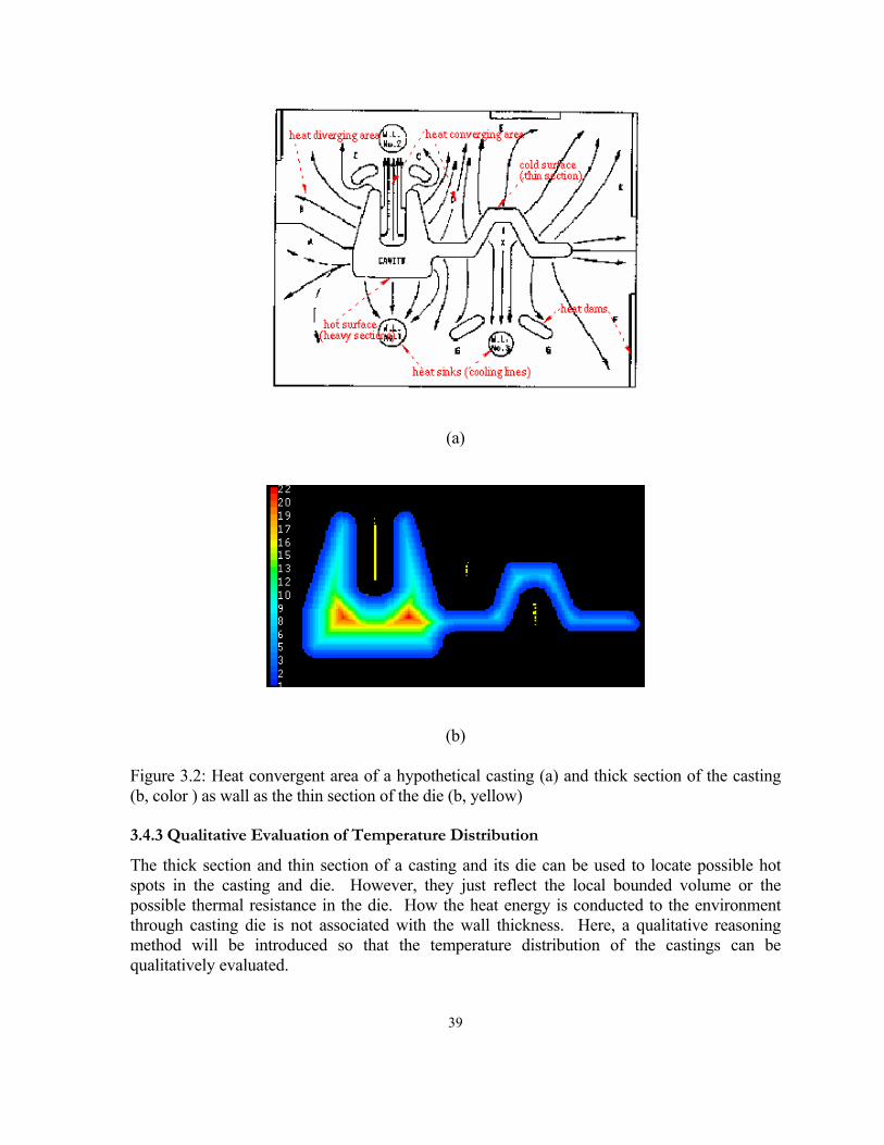
39

(a)

(b)

Figure 3.2: Heat convergent area of a hypothetical casting (a) and thick section of the casting (b, color ) as wall as the thin section of the die (b, yellow)

3.4.3 Qualitative Evaluation of Temperature Distribution

The thick section and thin section of a casting and its die can be used to locate possible hot spots in the casting and die. However, they just reflect the local bounded volume or the possible thermal resistance in the die. How the heat energy is conducted to the environment through casting die is not associated with the wall thickness. Here, a qualitative reasoning method will be introduced so that the temperature distribution of the castings can be qualitatively evaluated.

40

Modeling of the heat transfer when a casting is cooled inside die is difficult task. For qualitative evaluation, a simple model of heat conduction was employed to model the heat conduction for qualitatively evaluating the casting’s ejection temperature. The boundary-value problem of the temperature distribution of castings can be modeled as the following boundary-value problem:

Σ∈=

Σ∈=+∂∂∂∂

=∇

2

1

2

on P if

on P if 0

B)P(F)P(T

BT)P(NnT)P(M

tTTκ

(3.49)

where, M(P) and N(P) are described functions independent of time, F(p) is the initial temperature distribution. Choosing different functions of M(p) and N(p), (3.49) can describe different heat transfer boundary conditions, such as conduction boundary condition, constant temperature boundary condition, insulated boundary condition, convection boundary condition, or the combinations of them. Clearly, the first boundary condition includes the case in which a portion BT of the surface kept at constant temperature (M = 0, N ≠ 0), a portion BH is perfectly insulated (M ≠ 0, N = 0), and a portion BC is exposed to an ambient at zero through a boundary conductance [M=k, N=H(M)] where BT+BC+BH=B.

If the boundary conditions are assumed time independent, the unknown temperature distribution T can be expressed as the form:

)t()M()t,M(T ΨΦ= (3.50)

Substitution of the this into the differential equation then yields two separate boundary value problems for Φ and Ψ respectively:

Σ=+∂∂

=∇

on 0 2

PforΦ)P(NnΦ)P(M

ΦΦ λ (3.51)

=Ψ

>=

)M(F)M(

Ψkdt

dΨ 0for t λ (3.52)

where λ is a constant, which is sometimes referred to as the separation constant.

The solution of Equation Eq.3.52 has basic solution of the form tke α− where α is a constant and have a relationship, 2αλ −= . Therefore, Eq.3.52 reflects the decay of the temperature spatial distribution, Φ, with time when castings cool from an initial temperature to the final steady state. The equation with respect to time usually may be easily solved; in particular, for a finite

41

body heating or cooling to a final uniform steady state (zero temperature throughout), the temperature distribution always may be written as in the form:

∑∞

=

−=1

),,(),,,(2

nn

tk zyxfetzyxT nα (3.53)

The boundary value problem for Φ, defined by equation 3.51 is a wave equation, and will have nontrivial solution only for certain particular discrete values of λn, n =1,2,3,… which are called the eigenvalues and the solutions corresponding to each λn are termed as eigenfunctions. The solutions of the wave equation, eigenfunctions, will entirely depend on the heat boundary conditions.

For a geometric reasoning approach to qualitatively evaluate the temperature distribution of castings, analytically solving the eigenvalue and eigenfunction problem is not preferred. Close examination of Eq.3.51 yields another explanation of the equation. Comparing the wave Eq.3.51 with Poisson’s equation, the function Φ on the left hand looks as if the source function of the Poisson’s equation. If the function Φ at right hand of Eq.3.51 is noted as Φ0, the wave equation can be seen as the Poisson’s equation:

Σ=+∂∂Φ=Φ∇

on 0

02

PforT)P(NnT)P(M

λ (3.54)

The determination of the solution of this equation is as difficult as the original one, unless further conditions are imposed that the boundary condition effect can be considered in another way or an infinite medium assumption can be made. In the approximation, a casting is analogized as being put in an enough large die so that the boundary condition’s influence can be ignored. If this is the case, the heat trap that partially reflects the boundary condition’s effect should be counted as heat sources. Based on the correlation between the wall thickness of castings and thermal mass, the distribution of the wall thickness can be used as the approximation of the function Φ0. The solution of the equation can be expressed as the form of volume potential:

∫∫∫Ω

=Φ0

0

MMM

dvr

),,(t)M( ςηξ (3.55)

where, t(ξ,η,ζ) is the thickness distribution of either the castings or die at M0(ξ,η,ζ). Through this volume potential, a relationship that links to the geometric information and the temperature distribution can be built. Comparing to the thickness-temperature approximation, the heat conduction effect during the cooling of castings has been approximately evaluated.

The evaluation of the integral Eq.3.55 is as difficult as solving the original differential equation Eq.3.54 unless the further approximations about the heat source function, the thickness

42

distribution of the castings and thin die thickness, are made. Therefore, two heat source entities, thermal skeleton and equivalent thermal sources, will be introduced. They will be discussed in next section.

Equivalent Thermal Heat Source Centers and Thermal Skeleton

To obtain the temperature distribution, the volume integral has to be evaluated. To make this integral easily evaluated, an entity called thermal equivalent point source can be introduced. According to the Fourier conduction law, the heat flux density vector q(M) at point M, which is defined as the heat energy loss at the point per unit time and unit surface, is proportional to local temperature gradient at this point:

)M(Tk)M( ∇=q (3.56)

The proportional coefficient is heat conductivity k. The amount of heat energy flowing out of a small surface surrounding a point M is given by:

bdsnQS∫∫ •= q (3.57)

where is q the flux vector, n is the outer normal. If Q is greater than zero, there is net energy flowing out of the point M and point M is defined as a point heat source. Therefore, at some points or regions, if their temperature is not smaller than their neighbors, q•n≥0 for all directions and the points or regions are heat sources. Applying this heat source definition to the wall thickness, this definition is exactly the same as the definition of the distance based geometric skeleton voxels of the castings. Therefore, a distance-based geometric skeleton voxel is referred as the thermal equivalent heat source. The linkage between the heat source and geometric skeleton can be built. The skeleton can be catalogued into subgroups according to their thickness value. A subgroup of the skeleton is referred as thermal skeleton corresponding to a certain temperature. The procedure discussed above is also suitable for the die thickness.

Temperature Pattern

As discussed in the asymptotic expression of the volume potential, at a great distance, the volume potential generated by a point sources can be approximated by S/R, where R is the distance from the point of observation to the center of the point source and S is the intensity of the point source. Therefore, the geometric center point source is defined as the equivalent thermal heat source center. It can be used in the qualitative evaluation of temperature. If the all skeleton voxels can be used as the point sources, the temperature pattern is the summation of the potentials created by each of the skeleton voxels, the equivalent thermal heat source centers, according to the asymptotic expression of potential (3.25):

∑+

=MN

i i

i

)z,y,x(rS

)z,y,x(T (3.58)

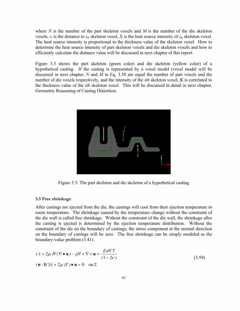
43

where N is the number of the part skeleton voxels and M is the number of the die skeleton voxels, ri is the distance to ith skeleton voxel, Si is the heat source intensity of ith skeleton voxel. The heat source intensity is proportional to the thickness value of the skeleton voxel. How to determine the heat source intensity of part skeleton voxels and die skeleton voxels and how to efficiently calculate the distance value will be discussed in next chapter of this report.

Figure 3.3 shows the part skeleton (green color) and die skeleton (yellow color) of a hypothetical casting. If the casting is represented by a voxel model (voxel model will be discussed in next chapter, N and M in Eq. 3.58 are equal the number of part voxels and the number of die voxels respectively, and the intensity of the ith skeleton voxel, Si is correlated to the thickness value of the ith skeleton voxel. This will be discussed in detail in next chapter, Geometric Reasoning of Casting Distortion.

Figure 3.3: The part skeleton and die skeleton of a hypothetical casting

3.5 Free shrinkage

After castings are ejected from the die, the castings will cool from their ejection temperature to room temperature. The shrinkage caused by the temperature change without the constraint of the die wall is called free shrinkage. Without the constraint of the die wall, the shrinkage after the casting is ejected is determined by the ejection temperature distribution. Without the constraint of the die on the boundary of castings, the stress component at the normal direction on the boundary of castings will be zero. The free shrinkage can be simply modeled as the boundary-value problem (3.41):

Σ=•+−∇

=×∇×∇−•∇∇+

on 0 23- 21

2

nIσ

uu

)T)(()(

TE)()(

µλν

αµµλ (3.59)

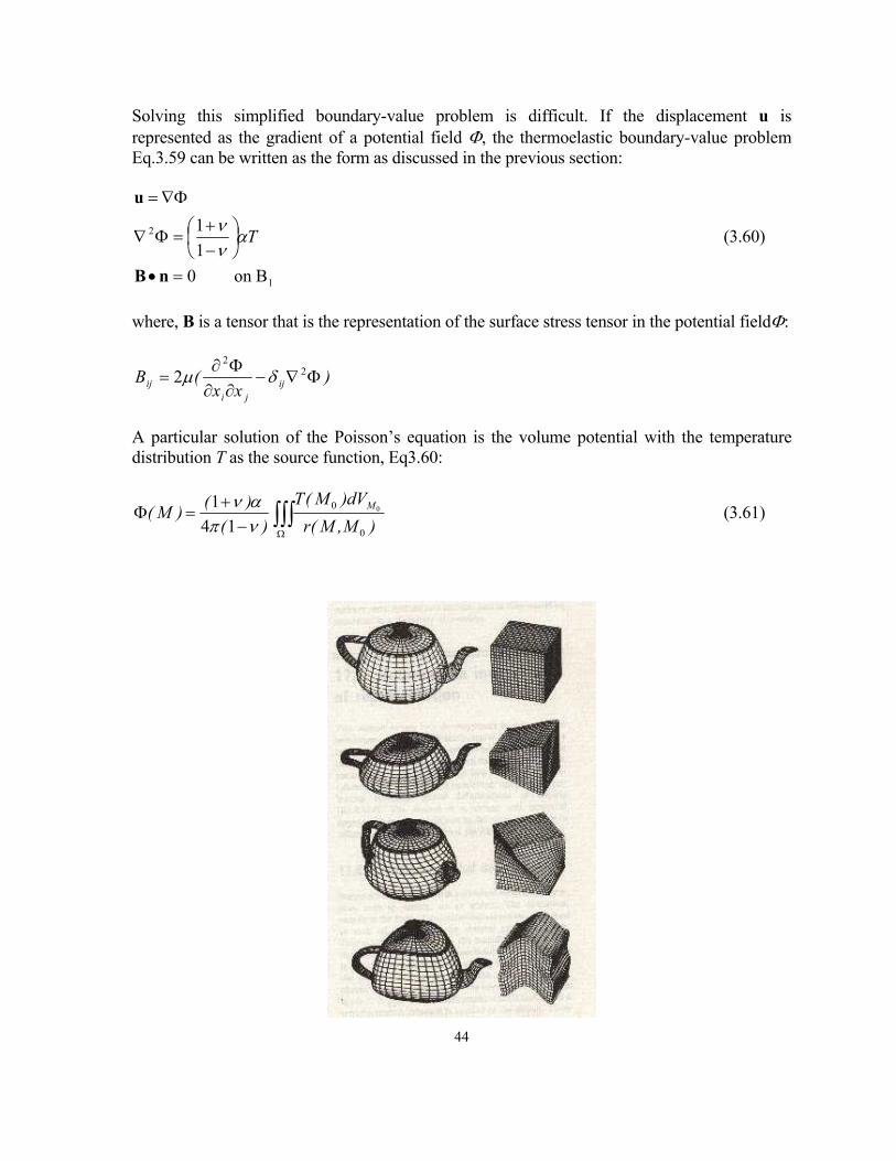
44

Solving this simplified boundary-value problem is difficult. If the displacement u is represented as the gradient of a potential field Φ, the thermoelastic boundary-value problem Eq.3.59 can be written as the form as discussed in the previous section:

1

2

Bon 011

=•

−+

=Φ∇

Φ∇=

nB

u

Tανν (3.60)

where, B is a tensor that is the representation of the surface stress tensor in the potential fieldΦ:

)xx

(B ijji

ij Φ∇−∂∂Φ∂

= 22

2 δµ

A particular solution of the Poisson’s equation is the volume potential with the temperature distribution T as the source function, Eq3.60:

∫∫∫Ω−

+=Φ

)M,M(rdV)M(T

)()()M( M

0

0 0

141

νπαν (3.61)

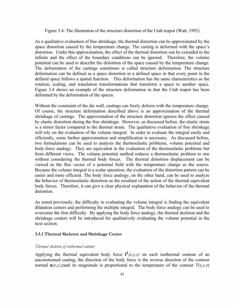
45

Figure 3.4: The illustration of the structure distortion of the Utah teapot (Watt, 1992)

As a qualitative evaluation of free shrinkage, the thermal distortion can be approximated by the space distortion caused by the temperature change. The casting is deformed with the space’s distortion. Under this approximation, the effect of the thermal distortion can be extended to the infinite and the effect of the boundary conditions can be ignored. Therefore, the volume potential can be used to describe the distortion of the space caused by the temperature change. The deformation of the castings sometimes is called structure deformation. The structure deformation can be defined as a space distortion in a defined space in that every point in the defined space follows a spatial function. This deformation has the same characteristics as the rotation, scaling, and translation transformations that transform a space to another space. Figure 3.4 shows an example of the structure deformation in that the Utah teapot has been deformed by the deformation of the spaces.

Without the constraint of the die wall, castings can freely deform with the temperature change. Of course, the structure deformation described above is an approximation of the thermal shrinkage of castings. The approximation of the structure distortion ignores the effect caused by elastic distortion during the free shrinkage. However, as discussed before, the elastic strain is a minor factor compared to the thermal strain. The qualitative evaluation of free shrinkage will rely on the evaluation of the volume integral. In order to evaluate the integral easily and efficiently, some further approximation and simplification is necessary. As discussed before, two formulations can be used to analysis the thermoelastic problems, volume potential and body-force analogy. They are equivalent in the evaluation of the thermoelastic problems but from different views. The volume potential method reduces a thermoelastic problem to one without considering the thermal body forces. The thermal distortion displacement can be viewed as the flux vector of a potential field with the temperature change as the source. Because the volume integral is a scalar operation, the evaluation of the distortion pattern can be easier and more efficient. The body force analogy, on the other hand, can be used to analyze the behavior of thermoelastic distortion as the resultant of the action of the thermal equivalent body forces. Therefore, it can give a clear physical explanation of the behavior of the thermal distortion.

As noted previously, the difficulty in evaluating the volume integral is finding the equivalent dilatation centers and performing the multiple integral. The body force analogy can be used to overcome the first difficulty. By applying the body force analogy, the thermal skeleton and the shrinkage centers will be introduced for qualitatively evaluating the volume potential in the next section.

3.5.1 Thermal Skeleton and Shrinkage Center

Thermal skeleton of isothermal contour

Applying the thermal equivalent body force fT(x,y,z) on each isothermal contour of an unconstrained casting, the direction of the body force is the inverse direction of the contour normal n(x,y,z)and its magnitude is proportional to the temperature of the contour T(x,y,z)

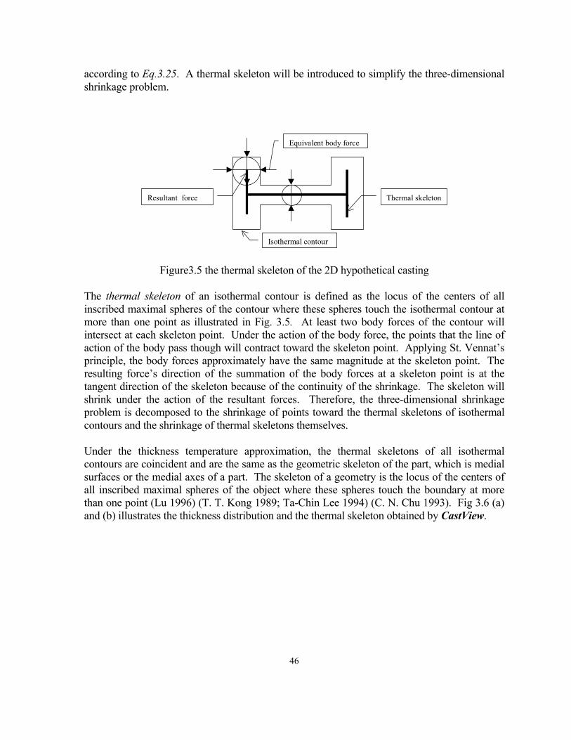
46

according to Eq.3.25. A thermal skeleton will be introduced to simplify the three-dimensional shrinkage problem.

Thermal skeleton

Isothermal contour

Equivalent body force

Resultant force

Figure3.5 the thermal skeleton of the 2D hypothetical casting

The thermal skeleton of an isothermal contour is defined as the locus of the centers of all inscribed maximal spheres of the contour where these spheres touch the isothermal contour at more than one point as illustrated in Fig. 3.5. At least two body forces of the contour will intersect at each skeleton point. Under the action of the body force, the points that the line of action of the body pass though will contract toward the skeleton point. Applying St. Vennat’s principle, the body forces approximately have the same magnitude at the skeleton point. The resulting force’s direction of the summation of the body forces at a skeleton point is at the tangent direction of the skeleton because of the continuity of the shrinkage. The skeleton will shrink under the action of the resultant forces. Therefore, the three-dimensional shrinkage problem is decomposed to the shrinkage of points toward the thermal skeletons of isothermal contours and the shrinkage of thermal skeletons themselves.

Under the thickness temperature approximation, the thermal skeletons of all isothermal contours are coincident and are the same as the geometric skeleton of the part, which is medial surfaces or the medial axes of a part. The skeleton of a geometry is the locus of the centers of all inscribed maximal spheres of the object where these spheres touch the boundary at more than one point (Lu 1996) (T. T. Kong 1989; Ta-Chin Lee 1994) (C. N. Chu 1993). Fig 3.6 (a) and (b) illustrates the thickness distribution and the thermal skeleton obtained by CastView.

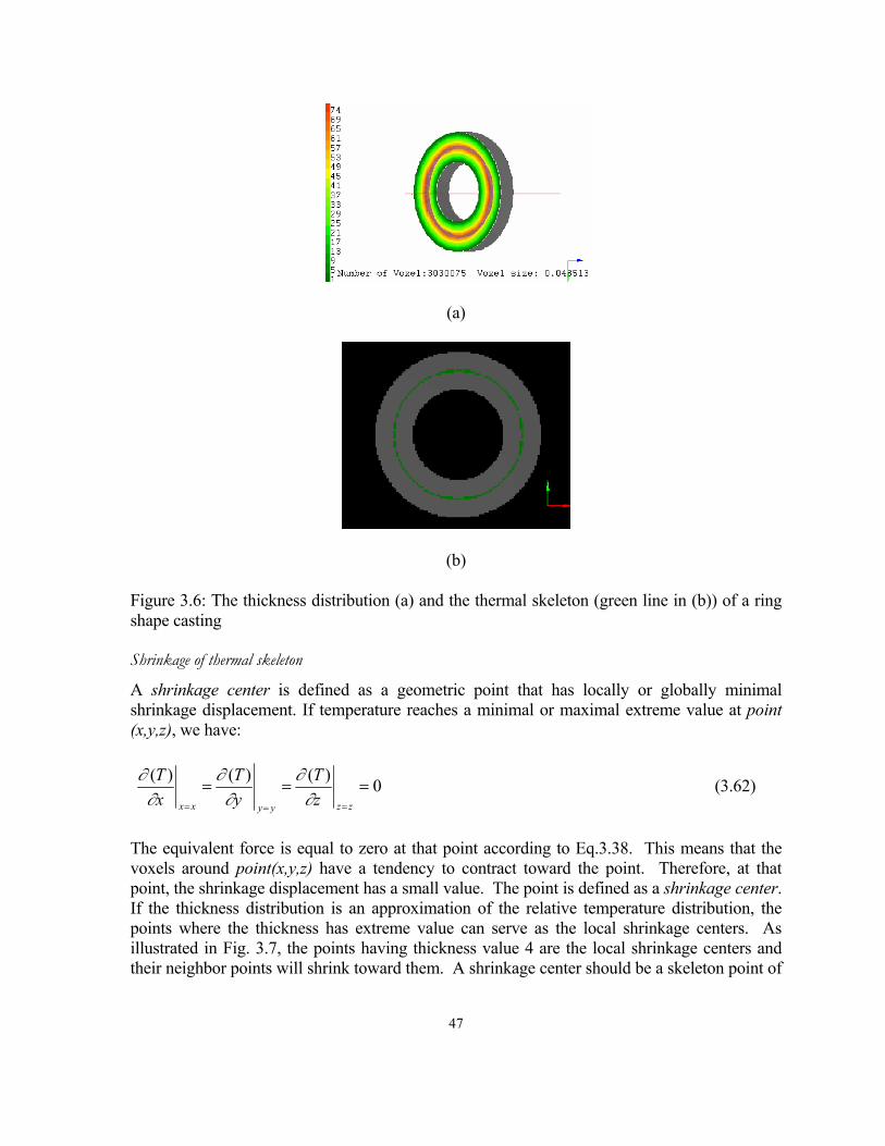
47

(a)

(b)

Figure 3.6: The thickness distribution (a) and the thermal skeleton (green line in (b)) of a ring shape casting

Shrinkage of thermal skeleton

A shrinkage center is defined as a geometric point that has locally or globally minimal shrinkage displacement. If temperature reaches a minimal or maximal extreme value at point (x,y,z), we have:

0)( )( )( ====== zzyyxx z

TyT

xT

∂∂

∂∂

∂∂ (3.62)

The equivalent force is equal to zero at that point according to Eq.3.38. This means that the voxels around point(x,y,z) have a tendency to contract toward the point. Therefore, at that point, the shrinkage displacement has a small value. The point is defined as a shrinkage center. If the thickness distribution is an approximation of the relative temperature distribution, the points where the thickness has extreme value can serve as the local shrinkage centers. As illustrated in Fig. 3.7, the points having thickness value 4 are the local shrinkage centers and their neighbor points will shrink toward them. A shrinkage center should be a skeleton point of

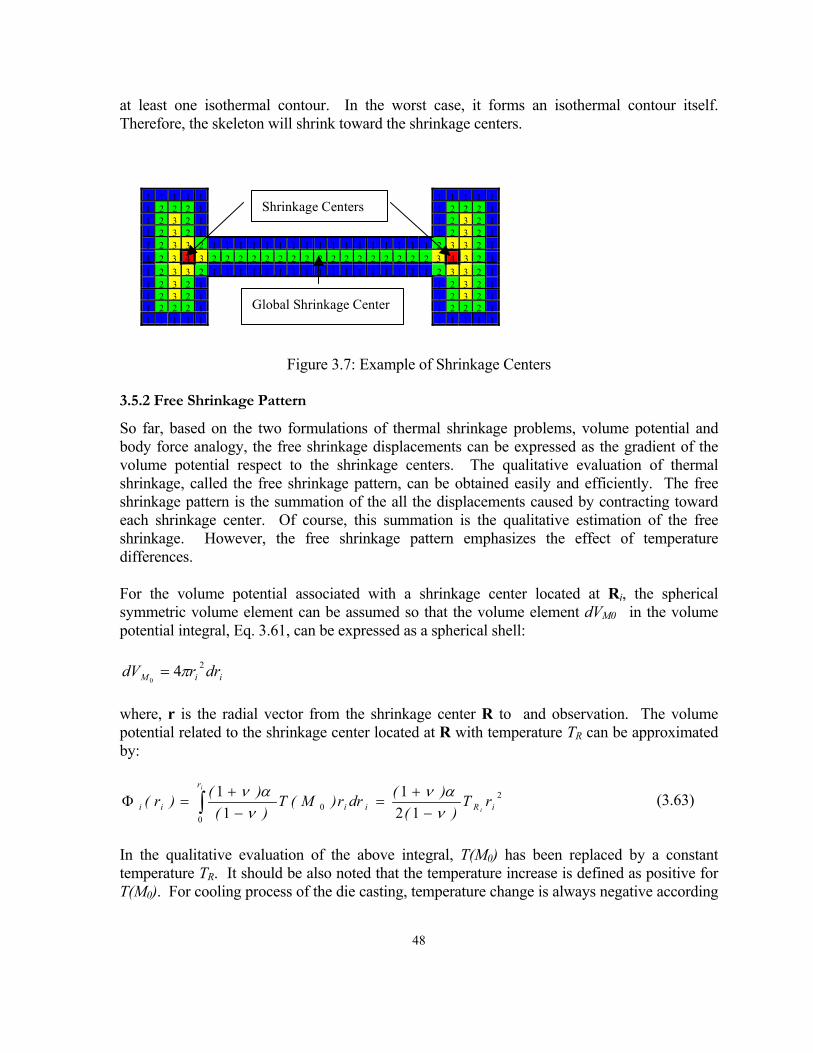
48

at least one isothermal contour. In the worst case, it forms an isothermal contour itself. Therefore, the skeleton will shrink toward the shrinkage centers.

1 1 1 1 1 1 1 1 1 11 2 2 2 1 1 2 2 2 11 2 3 2 1 1 2 3 2 11 2 3 2 1 1 2 3 2 11 2 3 3 2 1 1 1 1 1 1 1 1 1 1 1 1 1 1 1 1 1 2 3 3 2 11 2 3 4 3 2 2 2 2 2 2 2 2 2 2 2 2 2 2 2 2 2 3 4 3 2 11 2 3 3 2 1 1 1 1 1 1 1 1 1 1 1 1 1 1 1 1 1 2 3 3 2 11 2 3 2 1 1 2 3 2 11 2 3 2 1 1 2 3 2 11 2 2 2 1 1 2 2 2 11 1 1 1 1 1 1 1 1 1

Shrinkage Centers

Global Shrinkage Center

Figure 3.7: Example of Shrinkage Centers

3.5.2 Free Shrinkage Pattern

So far, based on the two formulations of thermal shrinkage problems, volume potential and body force analogy, the free shrinkage displacements can be expressed as the gradient of the volume potential respect to the shrinkage centers. The qualitative evaluation of thermal shrinkage, called the free shrinkage pattern, can be obtained easily and efficiently. The free shrinkage pattern is the summation of the all the displacements caused by contracting toward each shrinkage center. Of course, this summation is the qualitative estimation of the free shrinkage. However, the free shrinkage pattern emphasizes the effect of temperature differences.

For the volume potential associated with a shrinkage center located at Ri, the spherical symmetric volume element can be assumed so that the volume element dVM0 in the volume potential integral, Eq. 3.61, can be expressed as a spherical shell:

iiM drrdV 240

π=

where, r is the radial vector from the shrinkage center R to and observation. The volume potential related to the shrinkage center located at R with temperature TR can be approximated by:

2

00 12

11

1iR

r

iiii rT)(

)(drr)M(T)(

)()r(i

i

ναν

ναν

−+

=−+

=Φ ∫ (3.63)

In the qualitative evaluation of the above integral, T(M0) has been replaced by a constant temperature TR. It should be also noted that the temperature increase is defined as positive for T(M0). For cooling process of the die casting, temperature change is always negative according

49

to the sign definition. From Eq. 3.60, the displacement related to the shrinkage center can be obtained by the gradient operation:

iRR iiT

)()( ru

νν

−+

=11 (3.64)

The free shrinkage of a casting with the N shrinkage centers Ri, i=1,2,3,…will be:

∑=N

iRi

uu (3.65)

According to Eq.3.64 and 3.65, the evaluation of the free shrinkage pattern will involve determining the distances between shrinkage centers and the point of observations. In next chapter, several distance transform algorithms that can be efficiently calculated will be described.

3.6 Constrained Shrinkage

Both the temperature distribution and the constraint of the die wall determine the shrinkage before ejection. Therefore, relative to free shrinkage, the shrinkage is called constrained shrinkage. The constraint of the die wall will be represented as a displacement boundary condition. There is no shrinkage displacement component along the inverse normal direction of the constraint surface of the die wall if we assume that the die is rigid. The boundary-value problem, Eq. 3.41, for the constrained shrinkage can be written as:

Σ∈=•+Σ∈=

−∇

=×∇×∇−•∇∇+

2

1

on 0 23- on 0

212

B)T)((B

)(TE)()(

nIσu

uu

µλ

ναµµλ

(3.66)

where, B1 is the constrained surfaces and B2 is the free shrinkage surfaces. Their definitions and influences on the die-casting process were discussed in the previous chapter of this report.

The boundary value problem Eq.3.66 accounts both for the effect of the boundary constraint and for that of non-uniform temperature distributions. All the equations and boundary conditions to be satisfied are, however, linear. It is possible to divide the problem into two separate parts and thus to calculate the distortion as the sum of (1) those due to temperature alone and (2) those due to the boundary constraint in the absence of temperature:

cp uuu += (3.67)

50

where, up is the displacement due to the temperature distribution and uc is the displacement due to the boundary constraint.

The distortion due to temperature alone is obtained by the solution of Eq. 3.59 as in the previous section subject to the conditions:

Σ=•µ+λ

Σ∈=

ν−∇α

=×∇×∇µ−•∇∇µ+λ

on )T)(- (

B on )M( )(

TE)()(

p

pp

pp

023

212

1

nIσ

uu

uu

(3.68)

in place of those previously stated. A casting free of external tractions, for which Eq. 3.59 hold, is often referred to as a free shrinkage casting.

The distortion due to the die constraint can be expressed as a homogeneous equation and boundary conditions as described in Eq. 3.44:

Σ∈=•µ+λ

Σ∈=

=×∇×∇µ−•∇∇µ+λ

2

1

023

02

B on )T)(- (

B on )M(- )()(

c

pc

cc

nIσ

uuuu

(3.69)

Equivalently, the boundary condition, Σ∈= 1B on )M(- pc uu , can be expressed as the existence of an equivalent surface force and the effect of the equivalent surface force counteracts the shrinkage displacement along the inverse direction of the constrained surfaces. The exchange between displacement boundary condition to force boundary condition is commonly used to solve constrained problems in elastic mechanics (Housner 1966). The solution corresponding to the constraint of the boundary in the absence of temperature will satisfy:

Σ∈=•+−=×∇×∇−•∇∇+

2on 0 23- 2

B)T)(()()(

nIσFuu

µλµµλ

(3.70)

where F is the equivalent force on the constrained surface, boundary B1, caused by the resistance of the displacements up obtained from part 1. According to Hooke’s law, F can be written as the form:

Φ∇−=−= KK auF (3.71)

where K is constant related to the elastic modulus E, Φ is the volume potential, Eq.3.61, obtained from free shrinkage distortion as described in previous section. Still considered as the

51

space distortion, the distortion due to the constraint of the die wall, constrained distortion, can be approximated by the solution:

Φ+

=Ψ∇

Ψ∇=

)(K

,c

µλ 22

u (3.72)

where, the constants λ and µ were defined in previous section, K is the linear spring constant, and Φ is the volume potential of free shrinkage distortion on the constrained surface. The solution of Eq.3.72 can be expressed as the volume potential:

∫∫Φ

+=Ψ

1

0

02 B

M

)M,M(rdS

)(K)M(

µλ (3.73)

3.6.1Constrained Shrinkage Pattern

The constrained distortion pattern, the qualitative evaluation of the distortion caused by the constraint of the die, can be expressed as the gradient of the volume potential, Eq.3.56. The same argument about the shrinkage centers as the free shrinkage pattern can be made. In the case of constrained distortion, the dilation centers are not shrinkage centers but the constrained surfaces. Therefore, the contribution of the constrained surface Si to the volume potential also can be expressed in the same form as the free shrinkage pattern:

ii

R )(K

iru

µλ 2+Φ

= (3.74)

where, Φi is the value of the free shrinkage volume potential on the constrained surface, ri is the shortest distance from the observation point to the constrained surface. Here, another approximation has been introduced. Since the constrained surface usually is not a point but a surface, the distance to surface is not well defined but the shortest distance to a surface is well defined. It will be seen in next chapter, the shortest distance to the constrained surface can be calculated easily and efficiently by distance transformations.

The constrained pattern for a casting will be the summation of the contributions of all the constrained surfaces:

∑=N

iRi

uu (3.75)

3.6.2 Extraction of constrained Surfaces

The shrinkage of castings in the presence of the die constraints will be the combination of two effects under the surface force boundary condition. One of them is the free shrinkage, as described in the previous section, which is determined only by ejection temperature. This

52

shrinkage causes the casting distortion and creates the mechanical load on the surfaces that constrains this shrinkage. The “load” is the equivalent surface force in the force boundary condition. The free shrinkage also creates a mechanism to extract the constrained surface. After freely shrinking, some casting surfaces that contact a die surface will create boundary forces, and therefore they are constrained surfaces. This mechanism will be employed in the next section to extract constrained surfaces and the distribution of the load can be used to estimate the ejection load. A geometric reasoning approach to qualitative evaluate the volume integral by means of distance transformation will be discussed in next chapter of this report

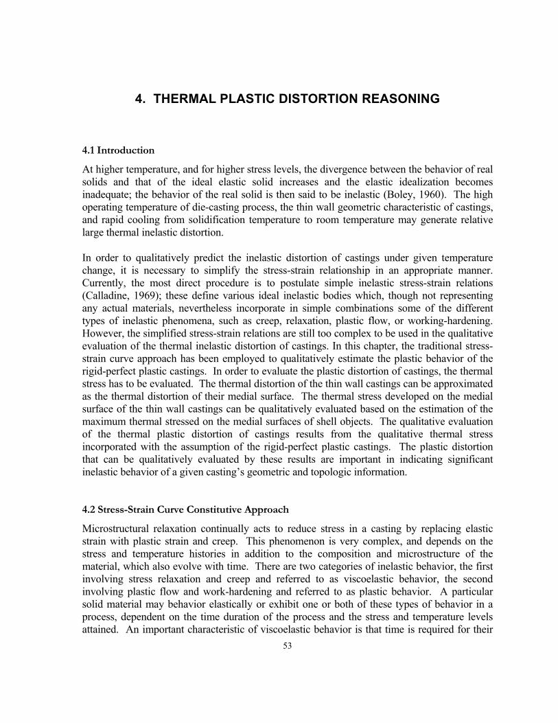
53

4. THERMAL PLASTIC DISTORTION REASONING

4.1 Introduction

At higher temperature, and for higher stress levels, the divergence between the behavior of real solids and that of the ideal elastic solid increases and the elastic idealization becomes inadequate; the behavior of the real solid is then said to be inelastic (Boley, 1960). The high operating temperature of die-casting process, the thin wall geometric characteristic of castings, and rapid cooling from solidification temperature to room temperature may generate relative large thermal inelastic distortion.

In order to qualitatively predict the inelastic distortion of castings under given temperature change, it is necessary to simplify the stress-strain relationship in an appropriate manner. Currently, the most direct procedure is to postulate simple inelastic stress-strain relations (Calladine, 1969); these define various ideal inelastic bodies which, though not representing any actual materials, nevertheless incorporate in simple combinations some of the different types of inelastic phenomena, such as creep, relaxation, plastic flow, or working-hardening. However, the simplified stress-strain relations are still too complex to be used in the qualitative evaluation of the thermal inelastic distortion of castings. In this chapter, the traditional stress-strain curve approach has been employed to qualitatively estimate the plastic behavior of the rigid-perfect plastic castings. In order to evaluate the plastic distortion of castings, the thermal stress has to be evaluated. The thermal distortion of the thin wall castings can be approximated as the thermal distortion of their medial surface. The thermal stress developed on the medial surface of the thin wall castings can be qualitatively evaluated based on the estimation of the maximum thermal stressed on the medial surfaces of shell objects. The qualitative evaluation of the thermal plastic distortion of castings results from the qualitative thermal stress incorporated with the assumption of the rigid-perfect plastic castings. The plastic distortion that can be qualitatively evaluated by these results are important in indicating significant inelastic behavior of a given casting’s geometric and topologic information.

4.2 Stress-Strain Curve Constitutive Approach

Microstructural relaxation continually acts to reduce stress in a casting by replacing elastic strain with plastic strain and creep. This phenomenon is very complex, and depends on the stress and temperature histories in addition to the composition and microstructure of the material, which also evolve with time. There are two categories of inelastic behavior, the first involving stress relaxation and creep and referred to as viscoelastic behavior, the second involving plastic flow and work-hardening and referred to as plastic behavior. A particular solid material may behavior elastically or exhibit one or both of these types of behavior in a process, dependent on the time duration of the process and the stress and temperature levels attained. An important characteristic of viscoelastic behavior is that time is required for their

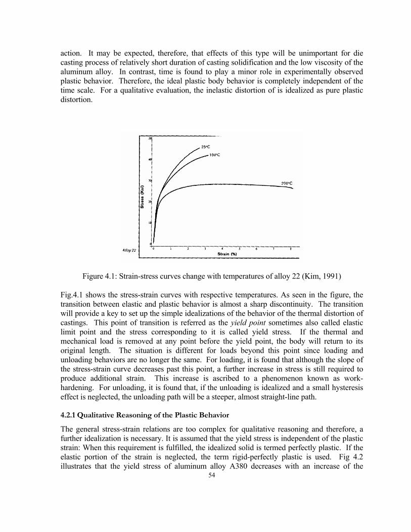
54

action. It may be expected, therefore, that effects of this type will be unimportant for die casting process of relatively short duration of casting solidification and the low viscosity of the aluminum alloy. In contrast, time is found to play a minor role in experimentally observed plastic behavior. Therefore, the ideal plastic body behavior is completely independent of the time scale. For a qualitative evaluation, the inelastic distortion of is idealized as pure plastic distortion.

Figure 4.1: Strain-stress curves change with temperatures of alloy 22 (Kim, 1991)

Fig.4.1 shows the stress-strain curves with respective temperatures. As seen in the figure, the transition between elastic and plastic behavior is almost a sharp discontinuity. The transition will provide a key to set up the simple idealizations of the behavior of the thermal distortion of castings. This point of transition is referred as the yield point sometimes also called elastic limit point and the stress corresponding to it is called yield stress. If the thermal and mechanical load is removed at any point before the yield point, the body will return to its original length. The situation is different for loads beyond this point since loading and unloading behaviors are no longer the same. For loading, it is found that although the slope of the stress-strain curve decreases past this point, a further increase in stress is still required to produce additional strain. This increase is ascribed to a phenomenon known as work-hardening. For unloading, it is found that, if the unloading is idealized and a small hysteresis effect is neglected, the unloading path will be a steeper, almost straight-line path.

4.2.1 Qualitative Reasoning of the Plastic Behavior

The general stress-strain relations are too complex for qualitative reasoning and therefore, a further idealization is necessary. It is assumed that the yield stress is independent of the plastic strain: When this requirement is fulfilled, the idealized solid is termed perfectly plastic. If the elastic portion of the strain is neglected, the term rigid-perfectly plastic is used. Fig 4.2 illustrates that the yield stress of aluminum alloy A380 decreases with an increase of the

55

temperature. When the temperature is high enough, a casting could be idealized as a rigid-perfect plastic body so that any thermal stress caused by temperature change will generate plastic distortion. For qualitative evaluating the plastic distortion, the assumption is made that the yield stress is low enough that any thermal stress will cause plastic distortion. The thermal plastic distortion is linearly proportional to the stress.

Figure 4.2: Yield stress changes with temperature (Kim, 1991)

The stress-strain curves for each temperature are assumed to consist of three linear sections, A-B, B-C, and C-D, as shown in Fig 4.3, where point B is the yield point. When castings are idealized as the rigid-perfectly plastic bodies, the three sections will be idealized as two linear sections, B-C and C-D, with plastic slopes E1 and E2. Consequently, the plastic strain is linearly proportion to stress:

σ=ε 1Ep

where εp denotes plastic strain. Although this assumption may not be entirely correct, it provides a limiting approximation of the thermal stress.

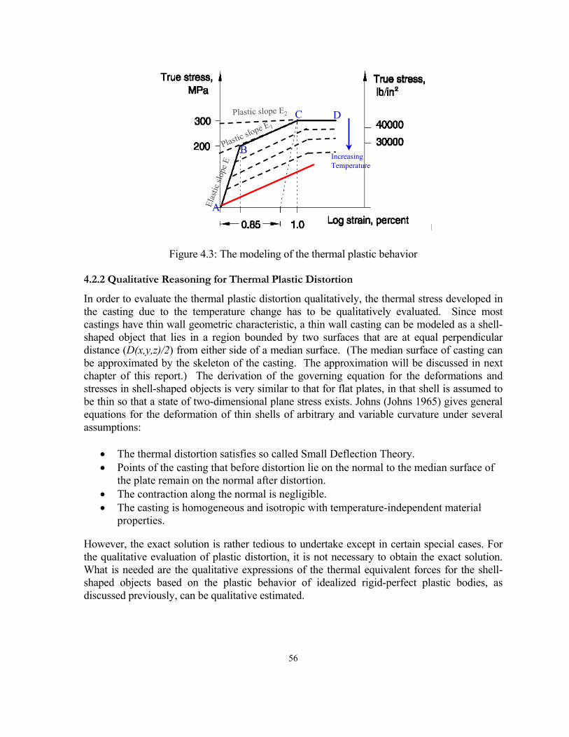
56

IncreasingTemperature

Plastic slope E1

Plastic slope E2

Elas

tic sl

ope E

IncreasingTemperature

Plastic slope E1

Plastic slope E2

Elas

tic sl

ope E

A

B

C D

Figure 4.3: The modeling of the thermal plastic behavior

4.2.2 Qualitative Reasoning for Thermal Plastic Distortion

In order to evaluate the thermal plastic distortion qualitatively, the thermal stress developed in the casting due to the temperature change has to be qualitatively evaluated. Since most castings have thin wall geometric characteristic, a thin wall casting can be modeled as a shell-shaped object that lies in a region bounded by two surfaces that are at equal perpendicular distance (D(x,y,z)/2) from either side of a median surface. (The median surface of casting can be approximated by the skeleton of the casting. The approximation will be discussed in next chapter of this report.) The derivation of the governing equation for the deformations and stresses in shell-shaped objects is very similar to that for flat plates, in that shell is assumed to be thin so that a state of two-dimensional plane stress exists. Johns (Johns 1965) gives general equations for the deformation of thin shells of arbitrary and variable curvature under several assumptions:

• The thermal distortion satisfies so called Small Deflection Theory. • Points of the casting that before distortion lie on the normal to the median surface of

the plate remain on the normal after distortion. • The contraction along the normal is negligible. • The casting is homogeneous and isotropic with temperature-independent material

properties. However, the exact solution is rather tedious to undertake except in certain special cases. For the qualitative evaluation of plastic distortion, it is not necessary to obtain the exact solution. What is needed are the qualitative expressions of the thermal equivalent forces for the shell-shaped objects based on the plastic behavior of idealized rigid-perfect plastic bodies, as discussed previously, can be qualitative estimated.

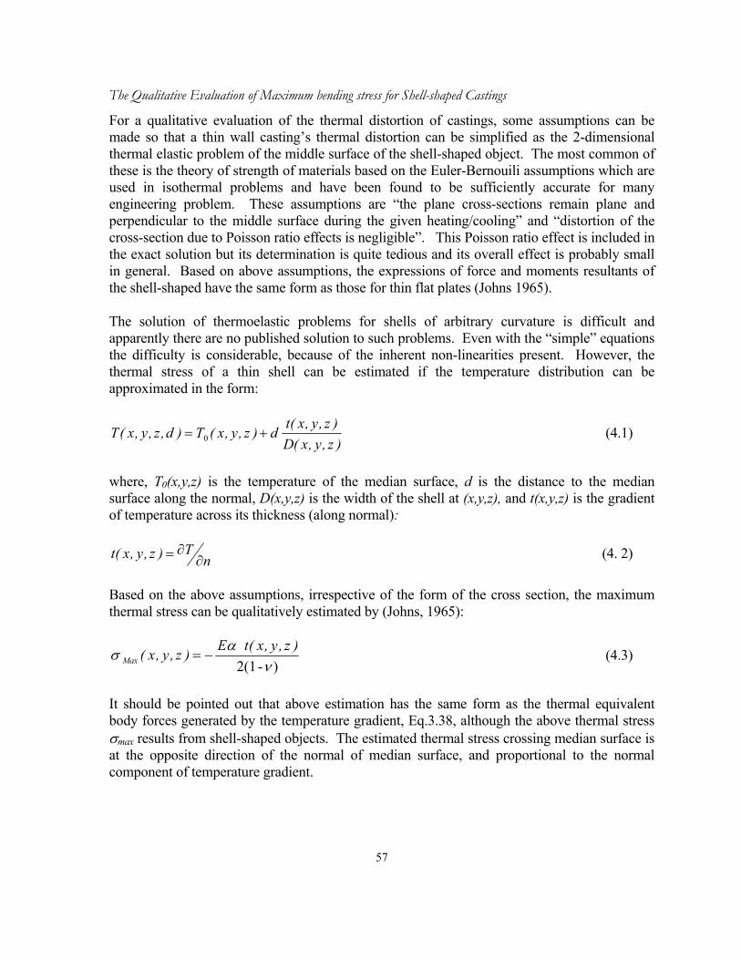
57

The Qualitative Evaluation of Maximum bending stress for Shell-shaped Castings

For a qualitative evaluation of the thermal distortion of castings, some assumptions can be made so that a thin wall casting’s thermal distortion can be simplified as the 2-dimensional thermal elastic problem of the middle surface of the shell-shaped object. The most common of these is the theory of strength of materials based on the Euler-Bernouili assumptions which are used in isothermal problems and have been found to be sufficiently accurate for many engineering problem. These assumptions are “the plane cross-sections remain plane and perpendicular to the middle surface during the given heating/cooling” and “distortion of the cross-section due to Poisson ratio effects is negligible”. This Poisson ratio effect is included in the exact solution but its determination is quite tedious and its overall effect is probably small in general. Based on above assumptions, the expressions of force and moments resultants of the shell-shaped have the same form as those for thin flat plates (Johns 1965).

The solution of thermoelastic problems for shells of arbitrary curvature is difficult and apparently there are no published solution to such problems. Even with the “simple” equations the difficulty is considerable, because of the inherent non-linearities present. However, the thermal stress of a thin shell can be estimated if the temperature distribution can be approximated in the form:

)z,y,x(D)z,y,x(td)z,y,x(T)d,z,y,x(T += 0 (4.1)

where, T0(x,y,z) is the temperature of the median surface, d is the distance to the median surface along the normal, D(x,y,z) is the width of the shell at (x,y,z), and t(x,y,z) is the gradient of temperature across its thickness (along normal):

nT)z,y,x(t ∂∂= (4. 2)

Based on the above assumptions, irrespective of the form of the cross section, the maximum thermal stress can be qualitatively estimated by (Johns, 1965):

)-2(1

να

σ)z,y,x(tE)z,y,x(Max −= (4.3)

It should be pointed out that above estimation has the same form as the thermal equivalent body forces generated by the temperature gradient, Eq.3.38, although the above thermal stress σmax results from shell-shaped objects. The estimated thermal stress crossing median surface is at the opposite direction of the normal of median surface, and proportional to the normal component of temperature gradient.

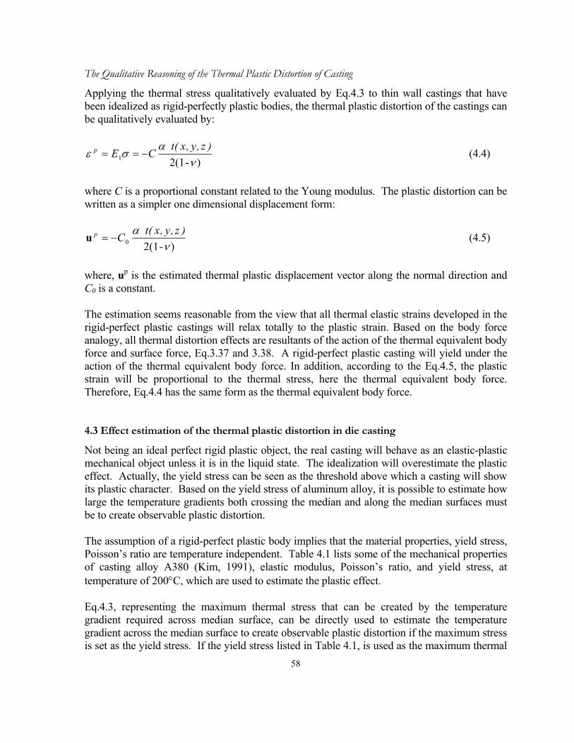
58

The Qualitative Reasoning of the Thermal Plastic Distortion of Casting

Applying the thermal stress qualitatively evaluated by Eq.4.3 to thin wall castings that have been idealized as rigid-perfectly plastic bodies, the thermal plastic distortion of the castings can be qualitatively evaluated by:

)-2(1

1 να

σε)z,y,x(tCEp −== (4.4)

where C is a proportional constant related to the Young modulus. The plastic distortion can be written as a simpler one dimensional displacement form:

)-2(1

0 να )z,y,x(tCp −=u (4.5)

where, up is the estimated thermal plastic displacement vector along the normal direction and C0 is a constant.

The estimation seems reasonable from the view that all thermal elastic strains developed in the rigid-perfect plastic castings will relax totally to the plastic strain. Based on the body force analogy, all thermal distortion effects are resultants of the action of the thermal equivalent body force and surface force, Eq.3.37 and 3.38. A rigid-perfect plastic casting will yield under the action of the thermal equivalent body force. In addition, according to the Eq.4.5, the plastic strain will be proportional to the thermal stress, here the thermal equivalent body force. Therefore, Eq.4.4 has the same form as the thermal equivalent body force.

4.3 Effect estimation of the thermal plastic distortion in die casting

Not being an ideal perfect rigid plastic object, the real casting will behave as an elastic-plastic mechanical object unless it is in the liquid state. The idealization will overestimate the plastic effect. Actually, the yield stress can be seen as the threshold above which a casting will show its plastic character. Based on the yield stress of aluminum alloy, it is possible to estimate how large the temperature gradients both crossing the median and along the median surfaces must be to create observable plastic distortion.

The assumption of a rigid-perfect plastic body implies that the material properties, yield stress, Poisson’s ratio are temperature independent. Table 4.1 lists some of the mechanical properties of casting alloy A380 (Kim, 1991), elastic modulus, Poisson’s ratio, and yield stress, at temperature of 200°C, which are used to estimate the plastic effect.

Eq.4.3, representing the maximum thermal stress that can be created by the temperature gradient required across median surface, can be directly used to estimate the temperature gradient across the median surface to create observable plastic distortion if the maximum stress is set as the yield stress. If the yield stress listed in Table 4.1, is used as the maximum thermal

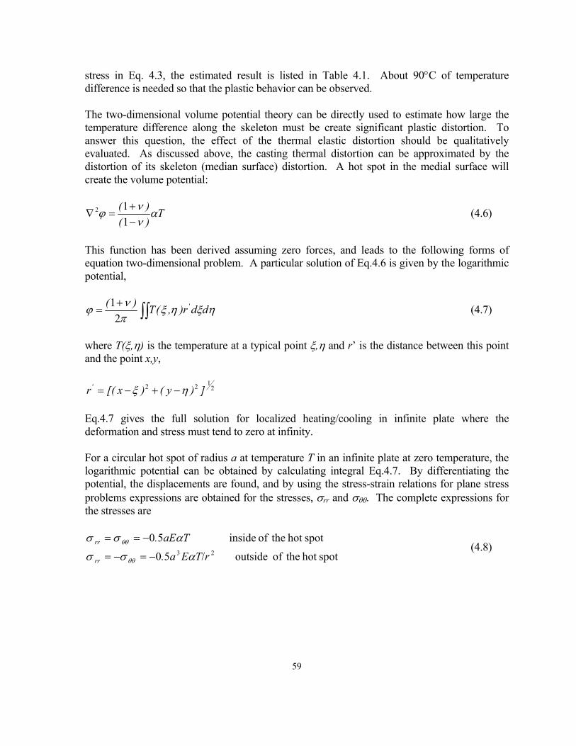
59

stress in Eq. 4.3, the estimated result is listed in Table 4.1. About 90°C of temperature difference is needed so that the plastic behavior can be observed.

The two-dimensional volume potential theory can be directly used to estimate how large the temperature difference along the skeleton must be create significant plastic distortion. To answer this question, the effect of the thermal elastic distortion should be qualitatively evaluated. As discussed above, the casting thermal distortion can be approximated by the distortion of its skeleton (median surface) distortion. A hot spot in the medial surface will create the volume potential:

T)()( α

ννϕ

−+

=∇112 (4.6)

This function has been derived assuming zero forces, and leads to the following forms of equation two-dimensional problem. A particular solution of Eq.4.6 is given by the logarithmic potential,

∫∫+

= ηξηξπνϕ ddr),(T)( '

21 (4.7)

where T(ξ,η) is the temperature at a typical point ξ,η and r’ is the distance between this point and the point x,y,

2122 ])y()x[(r' ηξ −+−=

Eq.4.7 gives the full solution for localized heating/cooling in infinite plate where the deformation and stress must tend to zero at infinity.

For a circular hot spot of radius a at temperature T in an infinite plate at zero temperature, the logarithmic potential can be obtained by calculating integral Eq.4.7. By differentiating the potential, the displacements are found, and by using the stress-strain relations for plane stress problems expressions are obtained for the stresses, σrr and σθθ. The complete expressions for the stresses are

spothot theof outside /50

spothot theof inside 5023 rTEa.

TaE.

rr

rr

ασσ

ασσ

θθ

θθ

−=−=

−== (4.8)

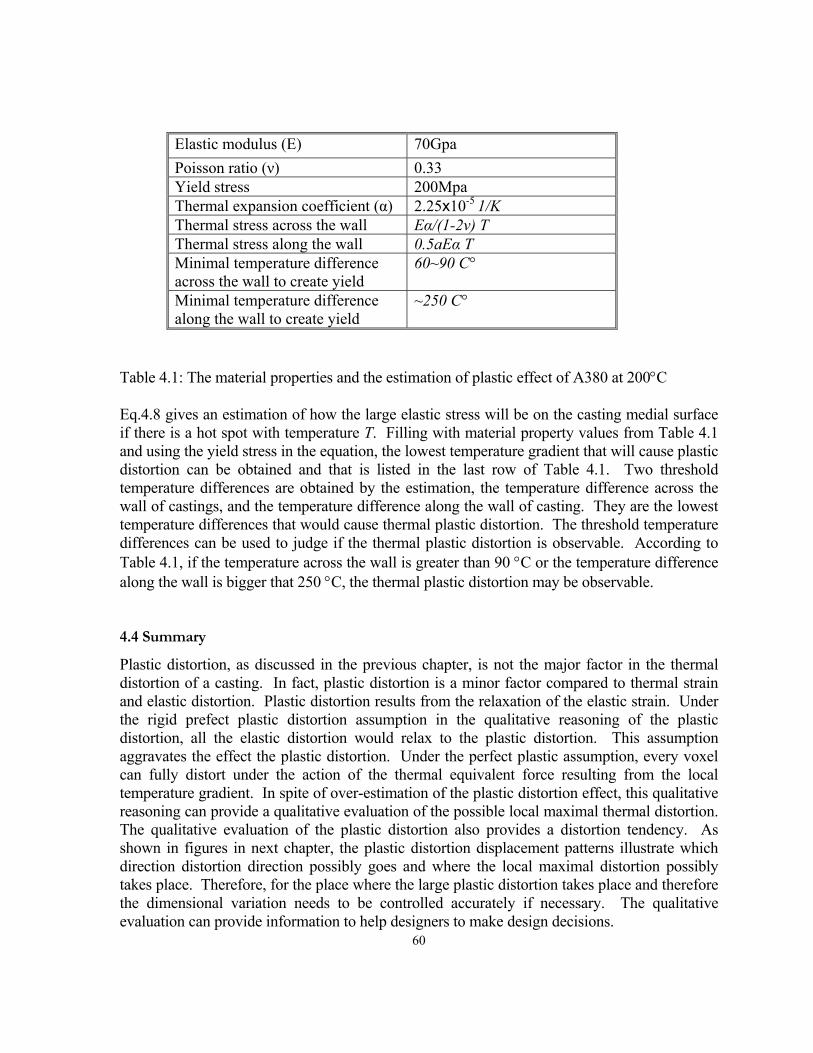
60

Elastic modulus (E) 70Gpa Poisson ratio (ν) 0.33 Yield stress 200Mpa Thermal expansion coefficient (α) 2.25х10-5 1/K Thermal stress across the wall Eα/(1-2ν) T Thermal stress along the wall 0.5aEα T Minimal temperature difference across the wall to create yield

60~90 C°

Minimal temperature difference along the wall to create yield

~250 C°

Table 4.1: The material properties and the estimation of plastic effect of A380 at 200°C

Eq.4.8 gives an estimation of how the large elastic stress will be on the casting medial surface if there is a hot spot with temperature T. Filling with material property values from Table 4.1 and using the yield stress in the equation, the lowest temperature gradient that will cause plastic distortion can be obtained and that is listed in the last row of Table 4.1. Two threshold temperature differences are obtained by the estimation, the temperature difference across the wall of castings, and the temperature difference along the wall of casting. They are the lowest temperature differences that would cause thermal plastic distortion. The threshold temperature differences can be used to judge if the thermal plastic distortion is observable. According to Table 4.1, if the temperature across the wall is greater than 90 °C or the temperature difference along the wall is bigger that 250 °C, the thermal plastic distortion may be observable.

4.4 Summary

Plastic distortion, as discussed in the previous chapter, is not the major factor in the thermal distortion of a casting. In fact, plastic distortion is a minor factor compared to thermal strain and elastic distortion. Plastic distortion results from the relaxation of the elastic strain. Under the rigid prefect plastic distortion assumption in the qualitative reasoning of the plastic distortion, all the elastic distortion would relax to the plastic distortion. This assumption aggravates the effect the plastic distortion. Under the perfect plastic assumption, every voxel can fully distort under the action of the thermal equivalent force resulting from the local temperature gradient. In spite of over-estimation of the plastic distortion effect, this qualitative reasoning can provide a qualitative evaluation of the possible local maximal thermal distortion. The qualitative evaluation of the plastic distortion also provides a distortion tendency. As shown in figures in next chapter, the plastic distortion displacement patterns illustrate which direction distortion direction possibly goes and where the local maximal distortion possibly takes place. Therefore, for the place where the large plastic distortion takes place and therefore the dimensional variation needs to be controlled accurately if necessary. The qualitative evaluation can provide information to help designers to make design decisions.

61

5. GEOMETRIC REASONING FOR CASTING DISTORTION

5.1 Introduction

In last two chapters, qualitative reasoning to evaluate several distortion patterns to predict the distortion tendency has been discussed. However, our final goal is developing a geometric analysis to represent and reason about the casting thermal distortion from the geometric and topological information of a given casting design. In this chapter, several geometric reasoning approaches will be discussed so that the distortion patterns developed in the qualitative reasoning of casting thermal distortion can be efficiently calculated. The voxel model is chosen as the geometric model for the geometric reasoning processes.

Qualitative evaluation of casting distortion is deeply involved in a key calculation, the calculation of the nearest distance to the “source” features, such as shrinkage centers, constrained surfaces, ejector pins. For a qualitative reasoning approach, it is required that the calculation should be efficient enough to support its applications in DFM. The most appropriate candidate to calculate the distance is a distance transform that was employed originally in the area of medical image processing. The approximate and discrete distance can be obtained by performing the distance transformation on an object represented as the voxel model. In this chapter, several algorithms and their implementation will be introduced and discussed. Among them, Euclidean distance transform can efficiently calculate the nearest Euclidean distance to a source features that consists of a group of voxels.

Based on the geometric reasoning approach, free shrinkage pattern, constrained distortion pattern, temperature pattern, and plastic distortion can be efficiently calculated. In order to qualitatively evaluate a thermal distortion, several special geometric reasoning algorithms were developed so that the skeleton of castings can be extracted and the distortion component on skeleton’s normal direction can be determined.

5.2 Part Model

Conventional CAD models, such as B-Rep, provide a reasonably robust environment in terms of geometric modeling and manipulation (Morterson 1995). However, it is quite difficult to derive diecastability-relevant geometric characteristics, consistently and efficiently from these models. Therefore, we have to seek other geometric models based on whether they can represent the geometry and topology of the interior of parts. In this proposed approach, the binary voxel-based model is used to support diecastability evaluation.

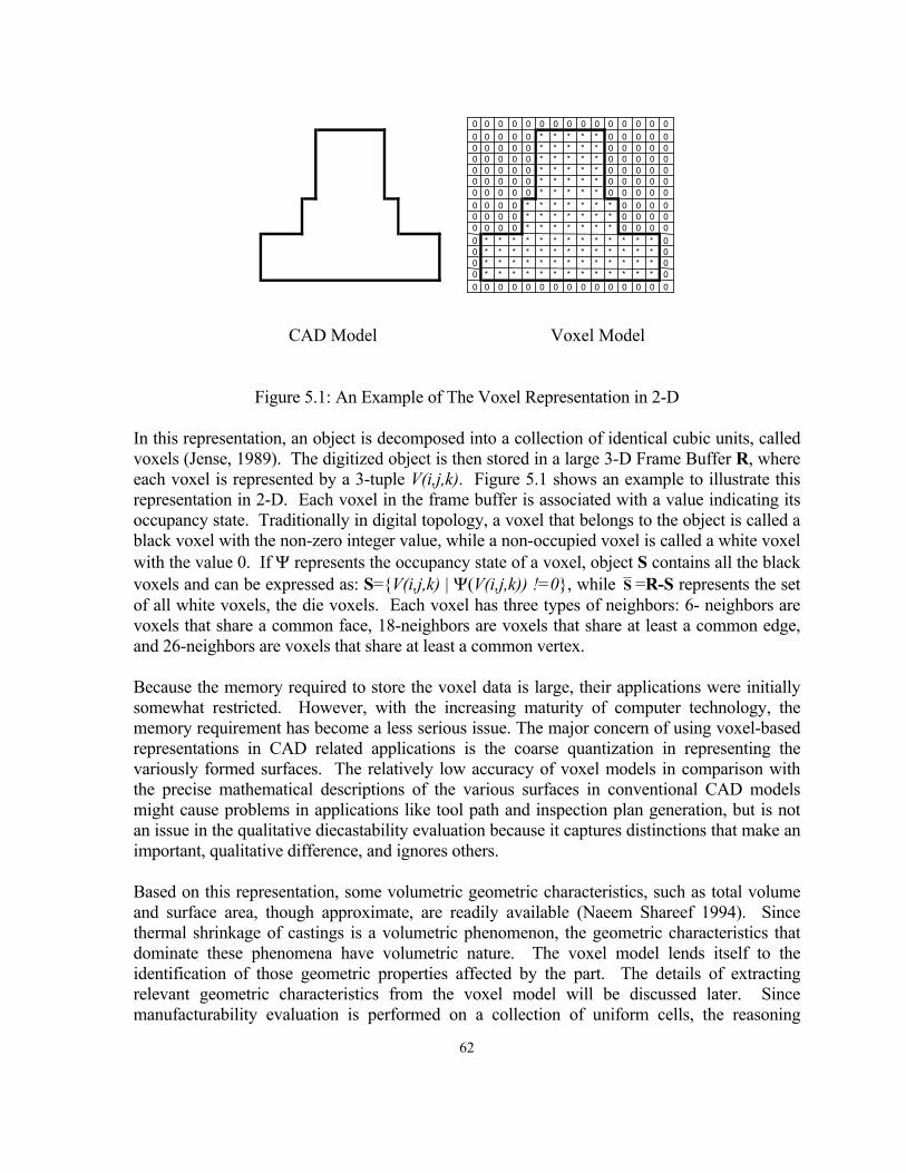
62

0 0 0 0 0 0 0 0 0 0 0 0 0 0 00 0 0 0 0 * * * * * 0 0 0 0 00 0 0 0 0 * * * * * 0 0 0 0 00 0 0 0 0 * * * * * 0 0 0 0 00 0 0 0 0 * * * * * 0 0 0 0 00 0 0 0 0 * * * * * 0 0 0 0 00 0 0 0 0 * * * * * 0 0 0 0 00 0 0 0 * * * * * * * 0 0 0 00 0 0 0 * * * * * * * 0 0 0 00 0 0 0 * * * * * * * 0 0 0 00 * * * * * * * * * * * * * 00 * * * * * * * * * * * * * 00 * * * * * * * * * * * * * 00 * * * * * * * * * * * * * 00 0 0 0 0 0 0 0 0 0 0 0 0 0 0

CAD Model Voxel Model

Figure 5.1: An Example of The Voxel Representation in 2-D

In this representation, an object is decomposed into a collection of identical cubic units, called voxels (Jense, 1989). The digitized object is then stored in a large 3-D Frame Buffer R, where each voxel is represented by a 3-tuple V(i,j,k). Figure 5.1 shows an example to illustrate this representation in 2-D. Each voxel in the frame buffer is associated with a value indicating its occupancy state. Traditionally in digital topology, a voxel that belongs to the object is called a black voxel with the non-zero integer value, while a non-occupied voxel is called a white voxel with the value 0. If Ψ represents the occupancy state of a voxel, object S contains all the black voxels and can be expressed as: S=V(i,j,k) | Ψ(V(i,j,k)) !=0, while S =R-S represents the set of all white voxels, the die voxels. Each voxel has three types of neighbors: 6- neighbors are voxels that share a common face, 18-neighbors are voxels that share at least a common edge, and 26-neighbors are voxels that share at least a common vertex.

Because the memory required to store the voxel data is large, their applications were initially somewhat restricted. However, with the increasing maturity of computer technology, the memory requirement has become a less serious issue. The major concern of using voxel-based representations in CAD related applications is the coarse quantization in representing the variously formed surfaces. The relatively low accuracy of voxel models in comparison with the precise mathematical descriptions of the various surfaces in conventional CAD models might cause problems in applications like tool path and inspection plan generation, but is not an issue in the qualitative diecastability evaluation because it captures distinctions that make an important, qualitative difference, and ignores others.

Based on this representation, some volumetric geometric characteristics, such as total volume and surface area, though approximate, are readily available (Naeem Shareef 1994). Since thermal shrinkage of castings is a volumetric phenomenon, the geometric characteristics that dominate these phenomena have volumetric nature. The voxel model lends itself to the identification of those geometric properties affected by the part. The details of extracting relevant geometric characteristics from the voxel model will be discussed later. Since manufacturability evaluation is performed on a collection of uniform cells, the reasoning

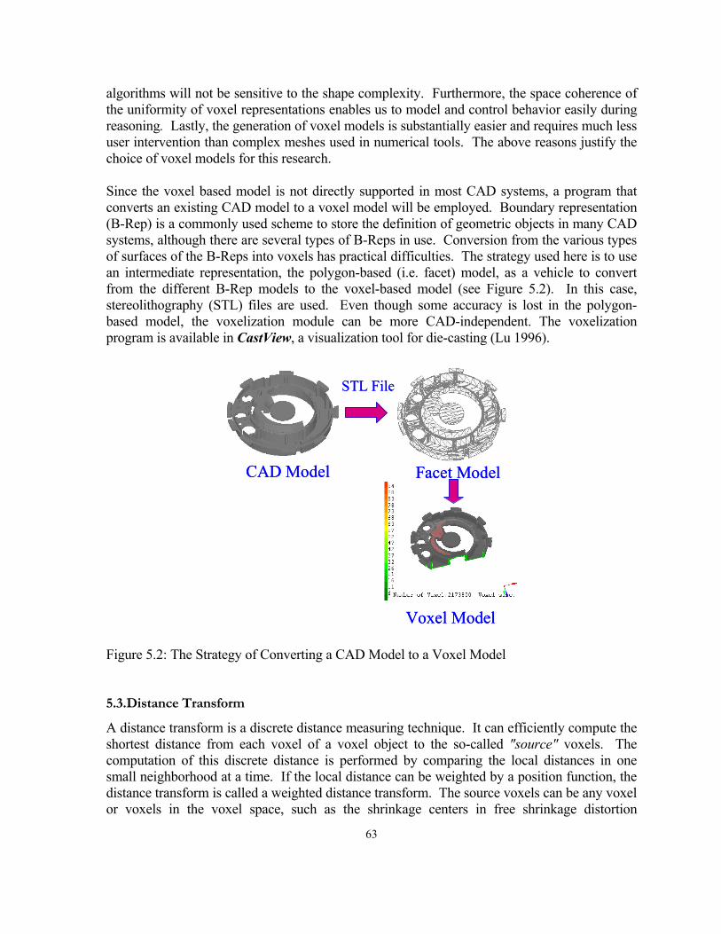
63

algorithms will not be sensitive to the shape complexity. Furthermore, the space coherence of the uniformity of voxel representations enables us to model and control behavior easily during reasoning. Lastly, the generation of voxel models is substantially easier and requires much less user intervention than complex meshes used in numerical tools. The above reasons justify the choice of voxel models for this research.

Since the voxel based model is not directly supported in most CAD systems, a program that converts an existing CAD model to a voxel model will be employed. Boundary representation (B-Rep) is a commonly used scheme to store the definition of geometric objects in many CAD systems, although there are several types of B-Reps in use. Conversion from the various types of surfaces of the B-Reps into voxels has practical difficulties. The strategy used here is to use an intermediate representation, the polygon-based (i.e. facet) model, as a vehicle to convert from the different B-Rep models to the voxel-based model (see Figure 5.2). In this case, stereolithography (STL) files are used. Even though some accuracy is lost in the polygon-based model, the voxelization module can be more CAD-independent. The voxelization program is available in CastView, a visualization tool for die-casting (Lu 1996).

CAD Model

STL File

Voxel Model

Facet ModelCAD Model

STL File

Voxel Model

Facet Model

Figure 5.2: The Strategy of Converting a CAD Model to a Voxel Model

5.3.Distance Transform

A distance transform is a discrete distance measuring technique. It can efficiently compute the shortest distance from each voxel of a voxel object to the so-called "source" voxels. The computation of this discrete distance is performed by comparing the local distances in one small neighborhood at a time. If the local distance can be weighted by a position function, the distance transform is called a weighted distance transform. The source voxels can be any voxel or voxels in the voxel space, such as the shrinkage centers in free shrinkage distortion

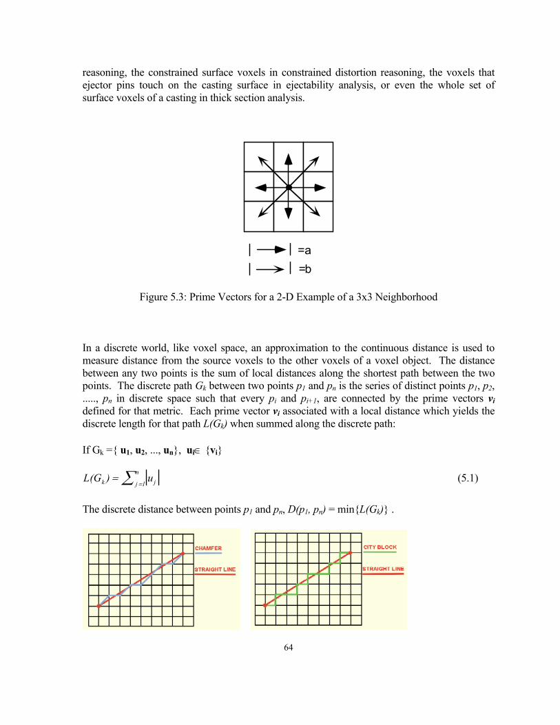
64

reasoning, the constrained surface voxels in constrained distortion reasoning, the voxels that ejector pins touch on the casting surface in ejectability analysis, or even the whole set of surface voxels of a casting in thick section analysis.

=a=b

Figure 5.3: Prime Vectors for a 2-D Example of a 3x3 Neighborhood

In a discrete world, like voxel space, an approximation to the continuous distance is used to measure distance from the source voxels to the other voxels of a voxel object. The distance between any two points is the sum of local distances along the shortest path between the two points. The discrete path Gk between two points p1 and pn is the series of distinct points p1, p2, ....., pn in discrete space such that every pi and pi+1, are connected by the prime vectors vi defined for that metric. Each prime vector vi associated with a local distance which yields the discrete length for that path L(Gk) when summed along the discrete path:

If Gk = u1, u2, ..., un, ui∈ vi

L(Gk ) = ujj=1

n∑ (5.1)

The discrete distance between points p1 and pn, D(p1, pn) = minL(Gk) .

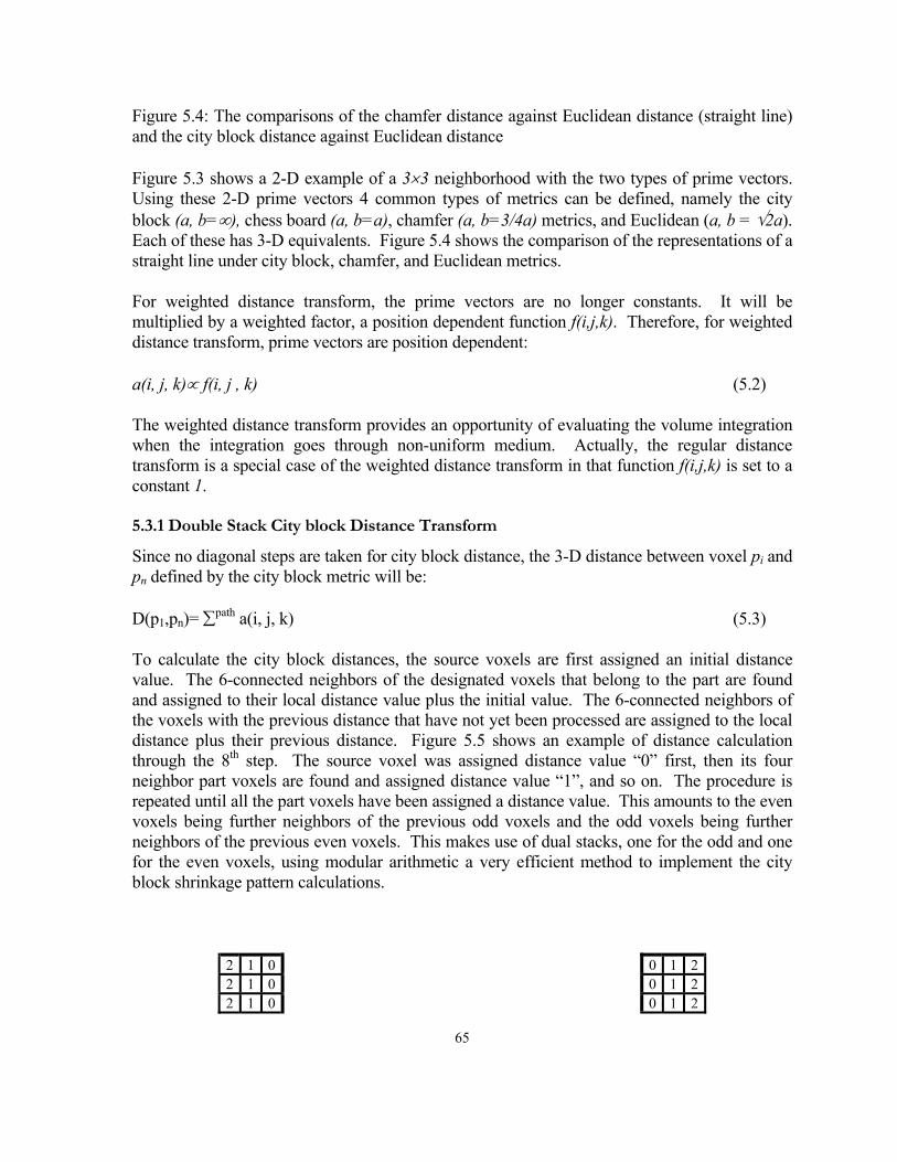
65

Figure 5.4: The comparisons of the chamfer distance against Euclidean distance (straight line) and the city block distance against Euclidean distance

Figure 5.3 shows a 2-D example of a 3×3 neighborhood with the two types of prime vectors. Using these 2-D prime vectors 4 common types of metrics can be defined, namely the city block (a, b=∞), chess board (a, b=a), chamfer (a, b=3/4a) metrics, and Euclidean (a, b = √2a). Each of these has 3-D equivalents. Figure 5.4 shows the comparison of the representations of a straight line under city block, chamfer, and Euclidean metrics.

For weighted distance transform, the prime vectors are no longer constants. It will be multiplied by a weighted factor, a position dependent function f(i,j,k). Therefore, for weighted distance transform, prime vectors are position dependent:

a(i, j, k)∝ f(i, j , k) (5.2)

The weighted distance transform provides an opportunity of evaluating the volume integration when the integration goes through non-uniform medium. Actually, the regular distance transform is a special case of the weighted distance transform in that function f(i,j,k) is set to a constant 1.

5.3.1 Double Stack City block Distance Transform

Since no diagonal steps are taken for city block distance, the 3-D distance between voxel pi and pn defined by the city block metric will be:

D(p1,pn)= ∑path a(i, j, k) (5.3)

To calculate the city block distances, the source voxels are first assigned an initial distance value. The 6-connected neighbors of the designated voxels that belong to the part are found and assigned to their local distance value plus the initial value. The 6-connected neighbors of the voxels with the previous distance that have not yet been processed are assigned to the local distance plus their previous distance. Figure 5.5 shows an example of distance calculation through the 8th step. The source voxel was assigned distance value “0” first, then its four neighbor part voxels are found and assigned distance value “1”, and so on. The procedure is repeated until all the part voxels have been assigned a distance value. This amounts to the even voxels being further neighbors of the previous odd voxels and the odd voxels being further neighbors of the previous even voxels. This makes use of dual stacks, one for the odd and one for the even voxels, using modular arithmetic a very efficient method to implement the city block shrinkage pattern calculations.

2 1 0 0 1 2 2 1 0 0 1 2 2 1 0 0 1 2

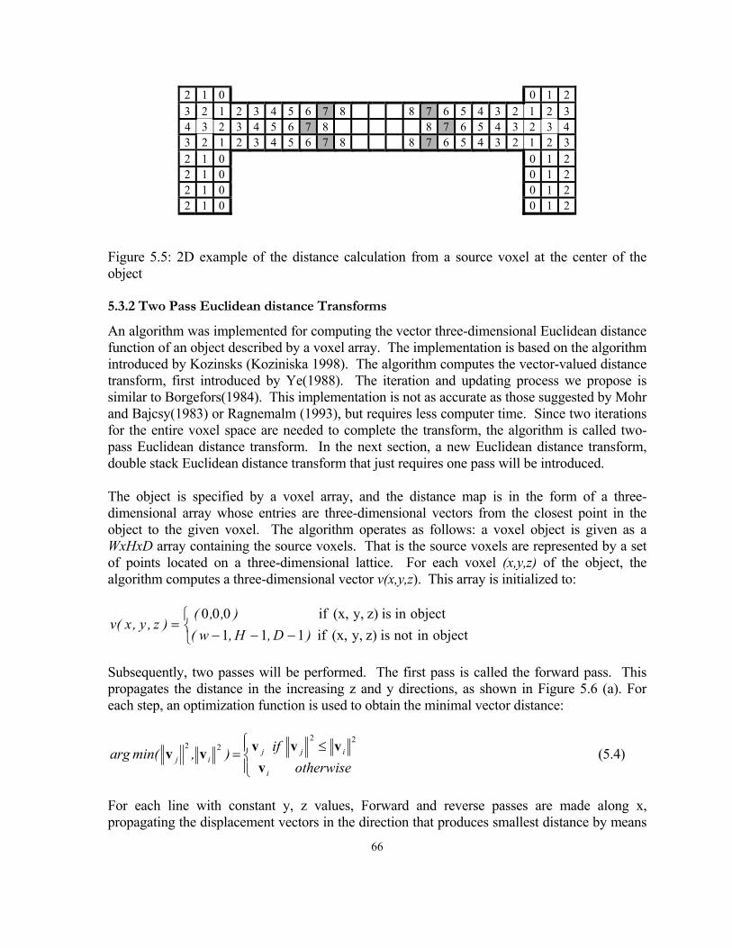
66

2 1 0 0 1 2 3 2 1 2 3 4 5 6 7 8 8 7 6 5 4 3 2 1 2 3 4 3 2 3 4 5 6 7 8 8 7 6 5 4 3 2 3 4 3 2 1 2 3 4 5 6 7 8 8 7 6 5 4 3 2 1 2 3 2 1 0 0 1 2 2 1 0 0 1 2 2 1 0 0 1 2 2 1 0 0 1 2

Figure 5.5: 2D example of the distance calculation from a source voxel at the center of the object

5.3.2 Two Pass Euclidean distance Transforms

An algorithm was implemented for computing the vector three-dimensional Euclidean distance function of an object described by a voxel array. The implementation is based on the algorithm introduced by Kozinsks (Koziniska 1998). The algorithm computes the vector-valued distance transform, first introduced by Ye(1988). The iteration and updating process we propose is similar to Borgefors(1984). This implementation is not as accurate as those suggested by Mohr and Bajcsy(1983) or Ragnemalm (1993), but requires less computer time. Since two iterations for the entire voxel space are needed to complete the transform, the algorithm is called two-pass Euclidean distance transform. In the next section, a new Euclidean distance transform, double stack Euclidean distance transform that just requires one pass will be introduced.

The object is specified by a voxel array, and the distance map is in the form of a three-dimensional array whose entries are three-dimensional vectors from the closest point in the object to the given voxel. The algorithm operates as follows: a voxel object is given as a WxHxD array containing the source voxels. That is the source voxels are represented by a set of points located on a three-dimensional lattice. For each voxel (x,y,z) of the object, the algorithm computes a three-dimensional vector v(x,y,z). This array is initialized to:

−−−=

objectin not is z)y,(x, if 111 object in is z)y,(x, if 000

)D,H,w(),,(

)z,y,x(v

Subsequently, two passes will be performed. The first pass is called the forward pass. This propagates the distance in the increasing z and y directions, as shown in Figure 5.6 (a). For each step, an optimization function is used to obtain the minimal vector distance:

≤=

otherwise if ),min(arg

i

ijjij

vvvvvv

2222

(5.4)

For each line with constant y, z values, Forward and reverse passes are made along x, propagating the displacement vectors in the direction that produces smallest distance by means

67

of the optimization function. Note that the minimum in each step of the pass is based on the Euclidean norm of the vectors. After the forward pass is completed, a second pass, called backward pass, is gone through, moving in the decreasing z and y directions as shown in Figure 5.6 (b). During the optimization step, vector distance function values are evaluated by array access. The Euclidean distance at x,y,z is computed from:

)vvv(round)z,y,x(d zyx222 ++=

Figure5.7shows the thick section of a cylindrical part based on city block, chamber, and Euclidean distance transforms. It clearly shows that the cylindrical symmetric thickness distribution is best from Euclidean distance, then chamfer distance, and then city block distance.

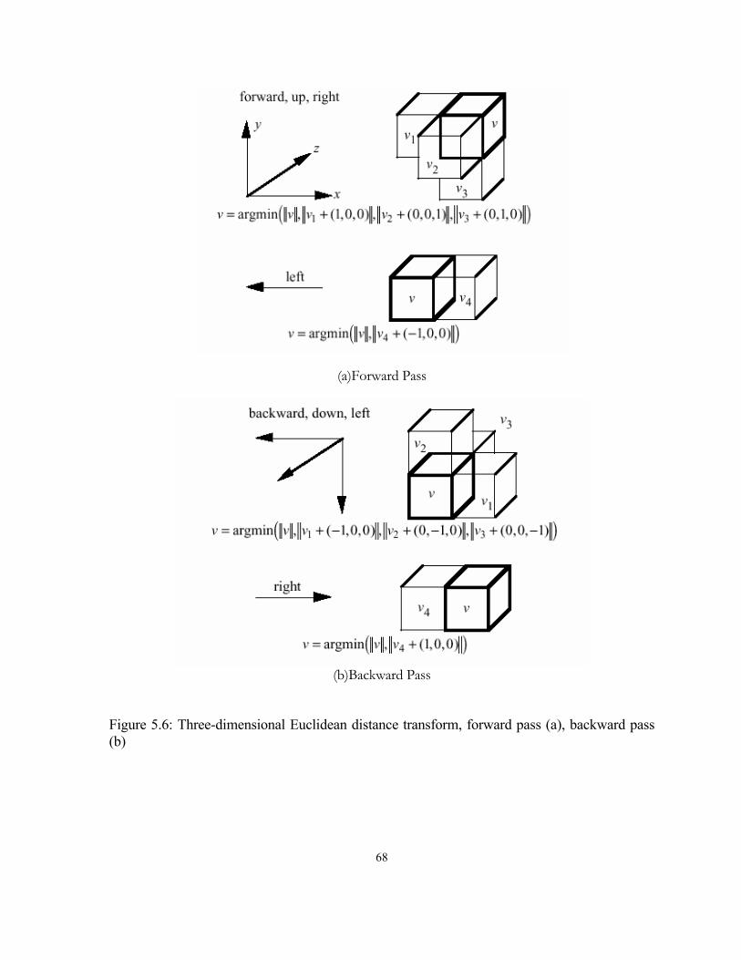
68

(a)Forward Pass

(b)Backward Pass

Figure 5.6: Three-dimensional Euclidean distance transform, forward pass (a), backward pass (b)

69

Similar two pass algorithms have been employed in CastView (Lu, 1997) to calculate both the chamfer and city block distances. The two-pass chamfer and city block distance transform also employs the forward pass and backward pass but no inner left and right pass. The other difference between the two-pass Euclidean distance transform and two pass chamfer and city block distance transform is that there are no Euclidean norm calculations in the chamfer and city block distance transform. Also, the distance transform is more efficient and costs less memory because no vector data is stored as intermediate results and no left and right inner passes are needed in the calculation. Figure5.7(b) and (c) are the thick section results obtained from CastView.

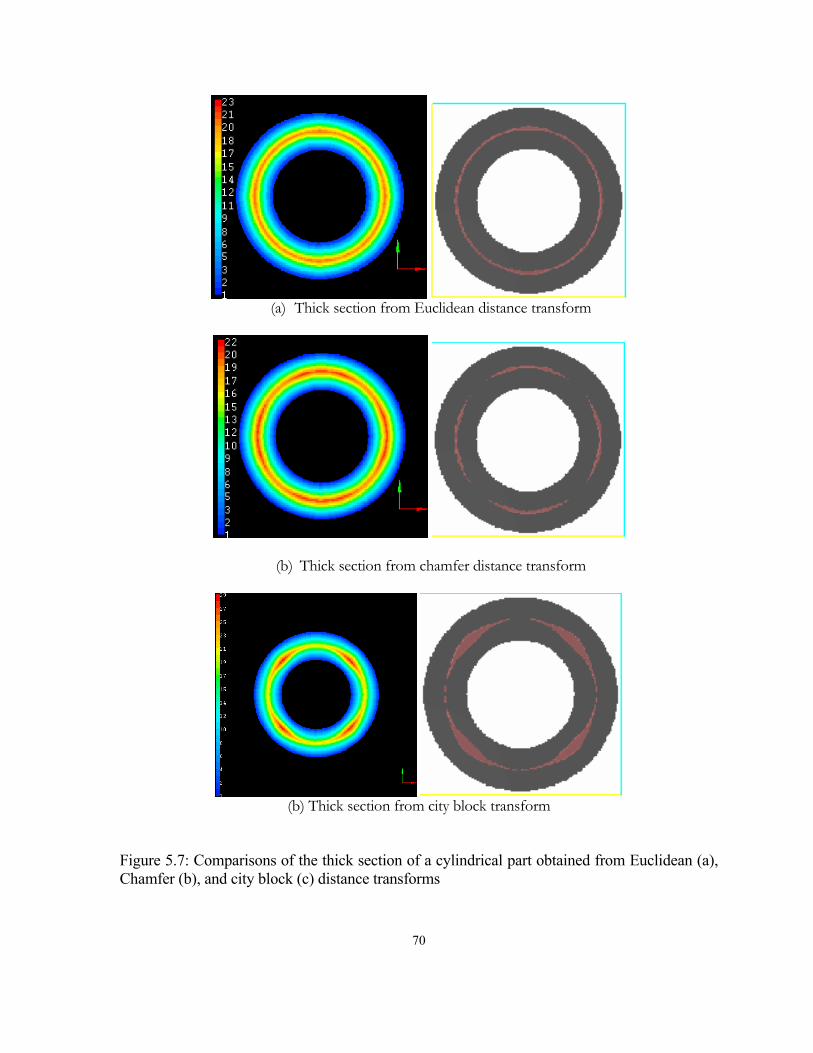
70

(a) Thick section from Euclidean distance transform

(b) Thick section from chamfer distance transform

(b) Thick section from city block transform

Figure 5.7: Comparisons of the thick section of a cylindrical part obtained from Euclidean (a), Chamfer (b), and city block (c) distance transforms

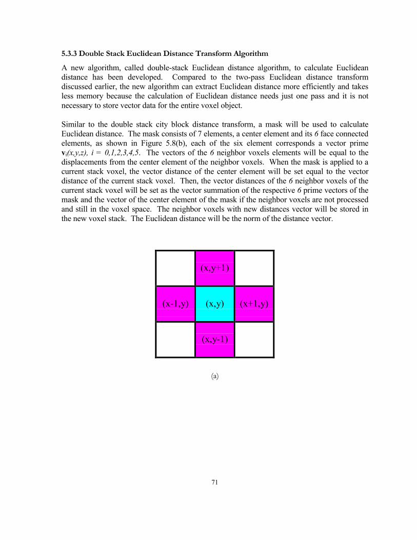
71

5.3.3 Double Stack Euclidean Distance Transform Algorithm

A new algorithm, called double-stack Euclidean distance algorithm, to calculate Euclidean distance has been developed. Compared to the two-pass Euclidean distance transform discussed earlier, the new algorithm can extract Euclidean distance more efficiently and takes less memory because the calculation of Euclidean distance needs just one pass and it is not necessary to store vector data for the entire voxel object.

Similar to the double stack city block distance transform, a mask will be used to calculate Euclidean distance. The mask consists of 7 elements, a center element and its 6 face connected elements, as shown in Figure 5.8(b), each of the six element corresponds a vector prime vi(x,y,z), i = 0,1,2,3,4,5. The vectors of the 6 neighbor voxels elements will be equal to the displacements from the center element of the neighbor voxels. When the mask is applied to a current stack voxel, the vector distance of the center element will be set equal to the vector distance of the current stack voxel. Then, the vector distances of the 6 neighbor voxels of the current stack voxel will be set as the vector summation of the respective 6 prime vectors of the mask and the vector of the center element of the mask if the neighbor voxels are not processed and still in the voxel space. The neighbor voxels with new distances vector will be stored in the new voxel stack. The Euclidean distance will be the norm of the distance vector.

(x,y+1)

(x-1,y)

(x,y)

(x+1,y)

(x,y-1)

(a)

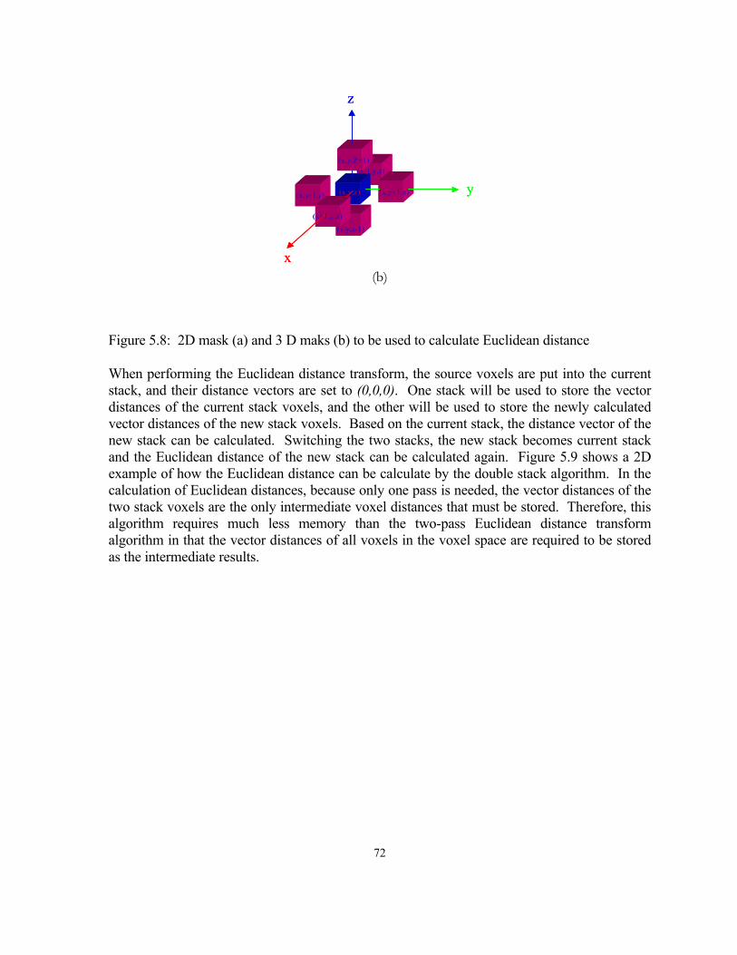
72

(x+1,y,z)

(x,y,Z+1)

(x,y+1,z)

(x-1,y,z)

(x,y-1,y)

(x,y,z-1)

(x,y,z)

x

y

z

(x+1,y,z)

(x,y,Z+1)

(x,y+1,z)

(x-1,y,z)

(x,y-1,y)

(x,y,z-1)

(x,y,z)

x

y

z

(b)

Figure 5.8: 2D mask (a) and 3 D maks (b) to be used to calculate Euclidean distance

When performing the Euclidean distance transform, the source voxels are put into the current stack, and their distance vectors are set to (0,0,0). One stack will be used to store the vector distances of the current stack voxels, and the other will be used to store the newly calculated vector distances of the new stack voxels. Based on the current stack, the distance vector of the new stack can be calculated. Switching the two stacks, the new stack becomes current stack and the Euclidean distance of the new stack can be calculated again. Figure 5.9 shows a 2D example of how the Euclidean distance can be calculate by the double stack algorithm. In the calculation of Euclidean distances, because only one pass is needed, the vector distances of the two stack voxels are the only intermediate voxel distances that must be stored. Therefore, this algorithm requires much less memory than the two-pass Euclidean distance transform algorithm in that the vector distances of all voxels in the voxel space are required to be stored as the intermediate results.

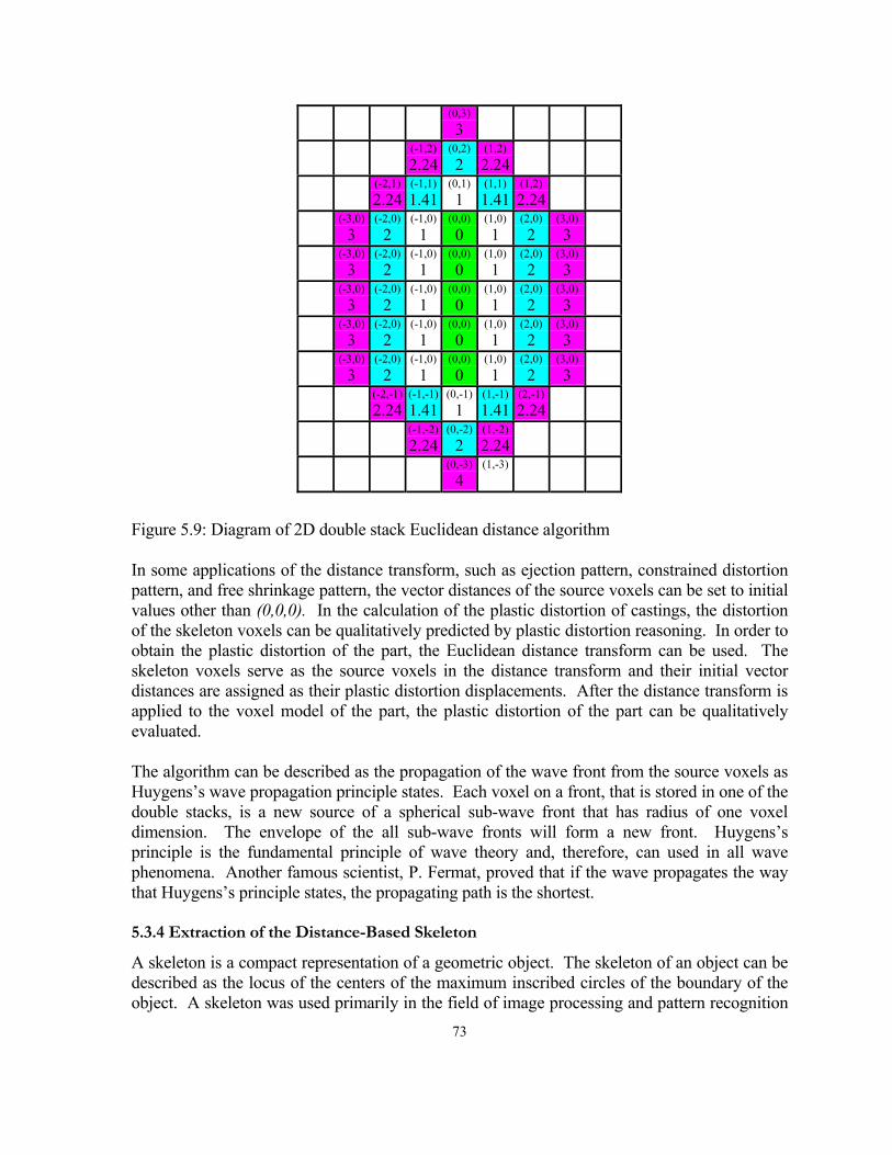
73

(0,3)3

(-1,2)2.24

(0,2)2

(1,2)2.24

(-2,1)2.24

(-1,1)1.41

(0,1)1

(1,1)1.41

(1,2)2.24

(-3,0)3

(-2,0)2

(-1,0)1

(0,0)0

(1,0)1

(2,0)2

(3,0)3

(-3,0)3

(-2,0)2

(-1,0)1

(0,0)0

(1,0)1

(2,0)2

(3,0)3

(-3,0)3

(-2,0)2

(-1,0)1

(0,0)0

(1,0)1

(2,0)2

(3,0)3

(-3,0)3

(-2,0)2

(-1,0)1

(0,0)0

(1,0)1

(2,0)2

(3,0)3

(-3,0)3

(-2,0)2

(-1,0)1

(0,0)0

(1,0)1

(2,0)2

(3,0)3

(-2,-1)2.24

(-1,-1)1.41

(0,-1)1

(1,-1)1.41

(2,-1)2.24

(-1,-2)2.24

(0,-2)2

(1,-2)2.24

(0,-3)4

(1,-3)

Figure 5.9: Diagram of 2D double stack Euclidean distance algorithm

In some applications of the distance transform, such as ejection pattern, constrained distortion pattern, and free shrinkage pattern, the vector distances of the source voxels can be set to initial values other than (0,0,0). In the calculation of the plastic distortion of castings, the distortion of the skeleton voxels can be qualitatively predicted by plastic distortion reasoning. In order to obtain the plastic distortion of the part, the Euclidean distance transform can be used. The skeleton voxels serve as the source voxels in the distance transform and their initial vector distances are assigned as their plastic distortion displacements. After the distance transform is applied to the voxel model of the part, the plastic distortion of the part can be qualitatively evaluated.

The algorithm can be described as the propagation of the wave front from the source voxels as Huygens’s wave propagation principle states. Each voxel on a front, that is stored in one of the double stacks, is a new source of a spherical sub-wave front that has radius of one voxel dimension. The envelope of the all sub-wave fronts will form a new front. Huygens’s principle is the fundamental principle of wave theory and, therefore, can used in all wave phenomena. Another famous scientist, P. Fermat, proved that if the wave propagates the way that Huygens’s principle states, the propagating path is the shortest.

5.3.4 Extraction of the Distance-Based Skeleton

A skeleton is a compact representation of a geometric object. The skeleton of an object can be described as the locus of the centers of the maximum inscribed circles of the boundary of the object. A skeleton was used primarily in the field of image processing and pattern recognition

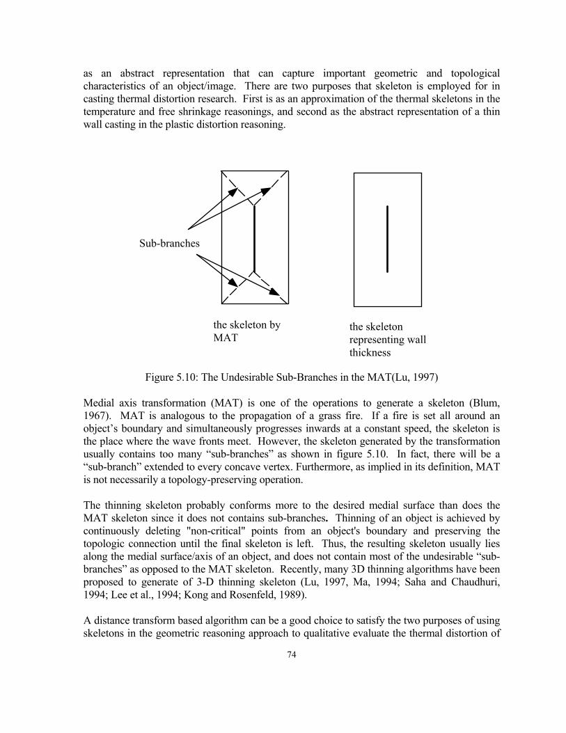
74

as an abstract representation that can capture important geometric and topological characteristics of an object/image. There are two purposes that skeleton is employed for in casting thermal distortion research. First is as an approximation of the thermal skeletons in the temperature and free shrinkage reasonings, and second as the abstract representation of a thin wall casting in the plastic distortion reasoning.

Sub-branches

the skeleton byMAT

the skeletonrepresenting wallthickness

Figure 5.10: The Undesirable Sub-Branches in the MAT(Lu, 1997)

Medial axis transformation (MAT) is one of the operations to generate a skeleton (Blum, 1967). MAT is analogous to the propagation of a grass fire. If a fire is set all around an object’s boundary and simultaneously progresses inwards at a constant speed, the skeleton is the place where the wave fronts meet. However, the skeleton generated by the transformation usually contains too many “sub-branches” as shown in figure 5.10. In fact, there will be a “sub-branch” extended to every concave vertex. Furthermore, as implied in its definition, MAT is not necessarily a topology-preserving operation.

The thinning skeleton probably conforms more to the desired medial surface than does the MAT skeleton since it does not contains sub-branches. Thinning of an object is achieved by continuously deleting "non-critical" points from an object's boundary and preserving the topologic connection until the final skeleton is left. Thus, the resulting skeleton usually lies along the medial surface/axis of an object, and does not contain most of the undesirable “sub- branches” as opposed to the MAT skeleton. Recently, many 3D thinning algorithms have been proposed to generate of 3-D thinning skeleton (Lu, 1997, Ma, 1994; Saha and Chaudhuri, 1994; Lee et al., 1994; Kong and Rosenfeld, 1989).

A distance transform based algorithm can be a good choice to satisfy the two purposes of using skeletons in the geometric reasoning approach to qualitative evaluate the thermal distortion of

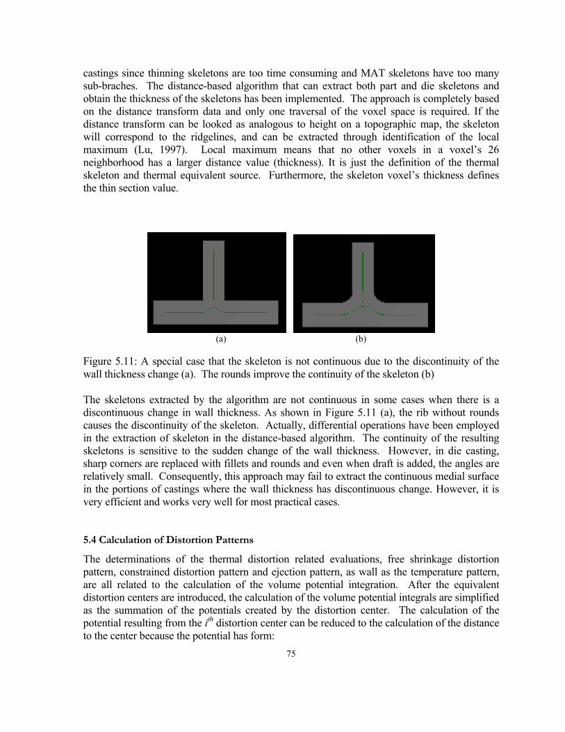
75

castings since thinning skeletons are too time consuming and MAT skeletons have too many sub-braches. The distance-based algorithm that can extract both part and die skeletons and obtain the thickness of the skeletons has been implemented. The approach is completely based on the distance transform data and only one traversal of the voxel space is required. If the distance transform can be looked as analogous to height on a topographic map, the skeleton will correspond to the ridgelines, and can be extracted through identification of the local maximum (Lu, 1997). Local maximum means that no other voxels in a voxel’s 26 neighborhood has a larger distance value (thickness). It is just the definition of the thermal skeleton and thermal equivalent source. Furthermore, the skeleton voxel’s thickness defines the thin section value.

(a) (b)

Figure 5.11: A special case that the skeleton is not continuous due to the discontinuity of the wall thickness change (a). The rounds improve the continuity of the skeleton (b)

The skeletons extracted by the algorithm are not continuous in some cases when there is a discontinuous change in wall thickness. As shown in Figure 5.11 (a), the rib without rounds causes the discontinuity of the skeleton. Actually, differential operations have been employed in the extraction of skeleton in the distance-based algorithm. The continuity of the resulting skeletons is sensitive to the sudden change of the wall thickness. However, in die casting, sharp corners are replaced with fillets and rounds and even when draft is added, the angles are relatively small. Consequently, this approach may fail to extract the continuous medial surface in the portions of castings where the wall thickness has discontinuous change. However, it is very efficient and works very well for most practical cases.

5.4 Calculation of Distortion Patterns

The determinations of the thermal distortion related evaluations, free shrinkage distortion pattern, constrained distortion pattern and ejection pattern, as wall as the temperature pattern, are all related to the calculation of the volume potential integration. After the equivalent distortion centers are introduced, the calculation of the volume potential integrals are simplified as the summation of the potentials created by the distortion center. The calculation of the potential resulting from the ith distortion center can be reduced to the calculation of the distance to the center because the potential has form:

76

2

0iR

r

iiii rFdRR)z,y,x(f)r(i

i

==Φ ∫ (5.5)

where, ri is the shortest distance to center i. The volume potential integral, the distortion pattern of the casting, can be approximated by adding the contributions of all distortion centers:

∑ ∑=Φ=ΦN

iiii )z,y,x(rF)z,y,x()z,y,x( 2 (5.6)

where, Fi is the intensity of ith distortion center, ri is the shortest distance to the ith distortion center obtained from the distance transform. Therefore, the volume potential is the weighted-summation of the distances. The weight factors are the intensities of the distortion centers. The distortion centers and their intensities will be discussed in the following sections.

5.4.1 Calculation of Free Shrinkage Pattern

The distance-based skeleton along with the thickness associated with each voxel of the skeleton should be extracted in order to obtain the free shrinkage pattern. As discussed in Free Shrinkage Reasoning section (section 3.5.1), if the wall thickness of a casting is used as an approximation of the ejection temperature of the casting, the thermal skeletons of the casting will be coincident to its distance-based geometric skeleton. The thickness associated with each skeleton voxel can approximate the temperature of the voxel.

To calculate free shrinkage, the free shrinkage centers have to be determined first. As discussed in previous chapter, all thermal skeletons are coincident with, and the same as, the thickness-based skeleton, under the assumption that the wall thickness is an approximation of the ejection temperature. The skeleton voxels will be categorized as sub-skeletons according to their thickness values. So, each sub-skeleton has the same thickness. Since each voxel of a sub-skeleton has the same temperature, the shrinkage center associated with the sub-skeleton will locate at the geometric center of the sub-skeleton according to the asymptotic expression for the volume potential. Therefore, the number of shrinkage centers, N, is equal to the number of different thickness values that the distance-based skeleton has.

Each shrinkage center will serve as the contraction center for calculating the volume potentials it creates. The source intensity of volume potential intensity of the shrinkage center, F, is its thickness value. Using each shrinkage center as the source voxel, the distance distribution of the part to the source voxel, ri, can be calculated by the two pass Euclidean distance transform discussed previously. The resultant distribution )z,y,x(iΦ , according to Eq. 3.63, is the potential created by the shrinkage center. The thickness-weighted summation of the potentials created by each shrinkage center is the shrinkage pattern of the casting.

Figure 5.12 (b) shows the free shrinkage pattern, obtained by the free shrinkage reasoning, of an example casting. The blue image shows in Figure 5.12 (c) is the shrinkage displacement pattern obtained by the free shrinkage reasoning. The free shrinkage pattern is the magnitude

77

distribution of the free shrinkage displacement pattern. The pattern shows two spots at the two sides of the boss, which means the free shrinkage displacement at the two spots has smallest and symmetric magnitude. The distance-based skeleton of the casting is shown in Figure 5.12 (a). The skeleton of the example casting has 6 different thickness values, 6, 5, 4, 3, 2, 1 for the voxel model used in the geometric reasoning. Therefore, 6 passed of the distance transformations are needed to calculated distance distributions respective to the 6 shrinkage centers. As pointed out, the double stack Euclidean distance transform can obtain the vector distance. So besides the free shrinkage pattern, the free shrinkage displacement also can be obtained.

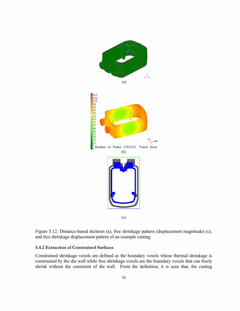
78

(a)

(b)

(c)

Figure 5.12: Distance-based skeleton (a), free shrinkage pattern (displacement magnitude) (c), and free shrinkage displacement pattern of an example casting

5.4.2 Extraction of Constrained Surfaces

Constrained shrinkage voxels are defined as the boundary voxels whose thermal shrinkage is constrained by the die wall while free shrinkage voxels are the boundary voxels that can freely shrink without the constraint of die wall. From the definition, it is seen that, the casting

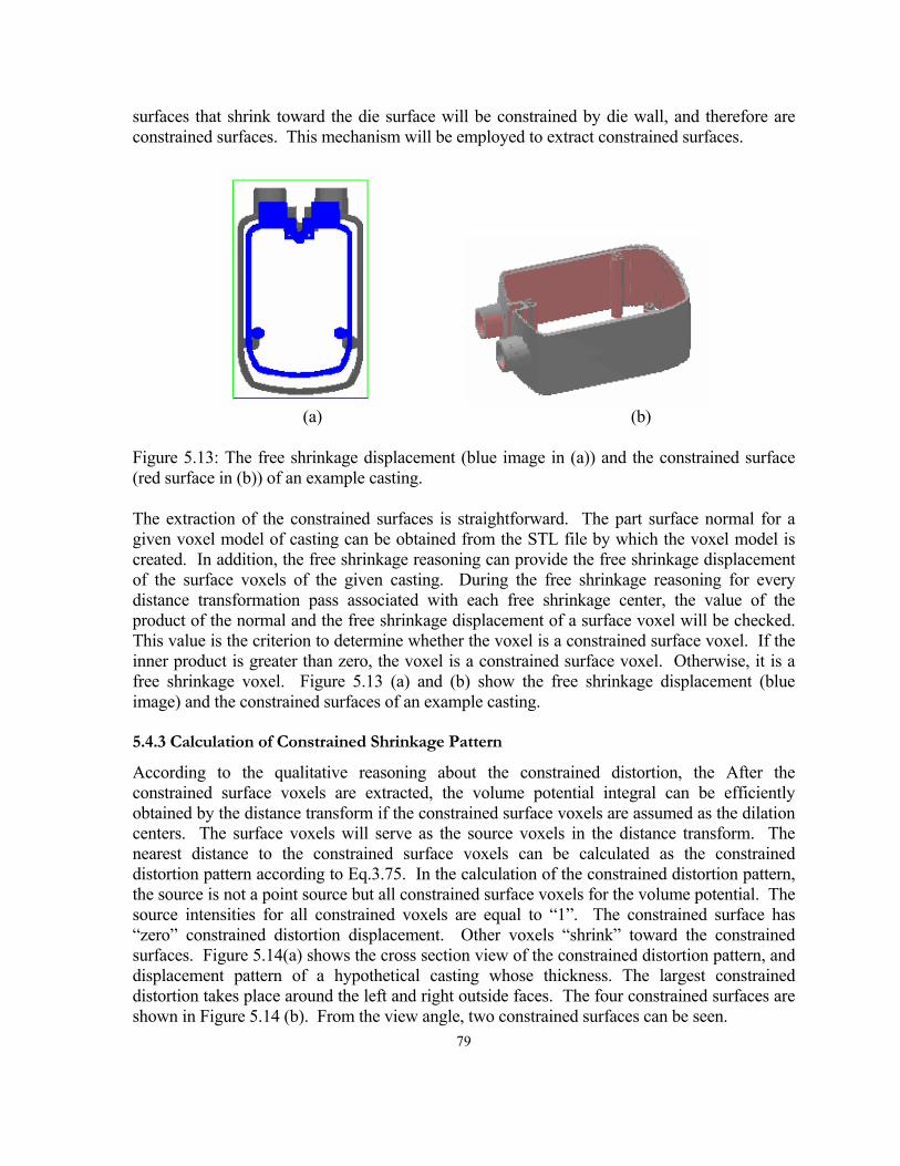
79

surfaces that shrink toward the die surface will be constrained by die wall, and therefore are constrained surfaces. This mechanism will be employed to extract constrained surfaces.

(a) (b)

Figure 5.13: The free shrinkage displacement (blue image in (a)) and the constrained surface (red surface in (b)) of an example casting.

The extraction of the constrained surfaces is straightforward. The part surface normal for a given voxel model of casting can be obtained from the STL file by which the voxel model is created. In addition, the free shrinkage reasoning can provide the free shrinkage displacement of the surface voxels of the given casting. During the free shrinkage reasoning for every distance transformation pass associated with each free shrinkage center, the value of the product of the normal and the free shrinkage displacement of a surface voxel will be checked. This value is the criterion to determine whether the voxel is a constrained surface voxel. If the inner product is greater than zero, the voxel is a constrained surface voxel. Otherwise, it is a free shrinkage voxel. Figure 5.13 (a) and (b) show the free shrinkage displacement (blue image) and the constrained surfaces of an example casting.

5.4.3 Calculation of Constrained Shrinkage Pattern

According to the qualitative reasoning about the constrained distortion, the After the constrained surface voxels are extracted, the volume potential integral can be efficiently obtained by the distance transform if the constrained surface voxels are assumed as the dilation centers. The surface voxels will serve as the source voxels in the distance transform. The nearest distance to the constrained surface voxels can be calculated as the constrained distortion pattern according to Eq.3.75. In the calculation of the constrained distortion pattern, the source is not a point source but all constrained surface voxels for the volume potential. The source intensities for all constrained voxels are equal to “1”. The constrained surface has “zero” constrained distortion displacement. Other voxels “shrink” toward the constrained surfaces. Figure 5.14(a) shows the cross section view of the constrained distortion pattern, and displacement pattern of a hypothetical casting whose thickness. The largest constrained distortion takes place around the left and right outside faces. The four constrained surfaces are shown in Figure 5.14 (b). From the view angle, two constrained surfaces can be seen.

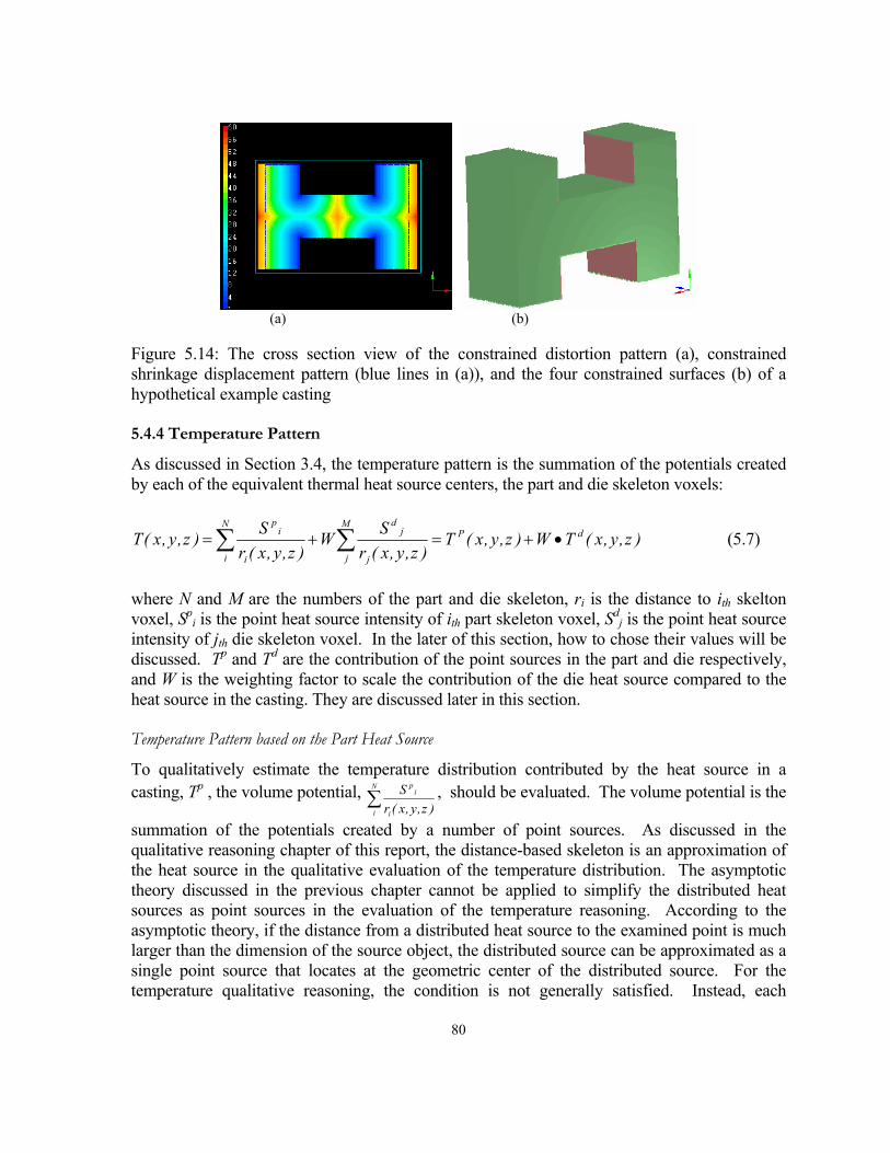
80

(a) (b)

Figure 5.14: The cross section view of the constrained distortion pattern (a), constrained shrinkage displacement pattern (blue lines in (a)), and the four constrained surfaces (b) of a hypothetical example casting

5.4.4 Temperature Pattern

As discussed in Section 3.4, the temperature pattern is the summation of the potentials created by each of the equivalent thermal heat source centers, the part and die skeleton voxels:

)z,y,x(TW)z,y,x(T)z,y,x(r

SW)z,y,x(r

S)z,y,x(T dPM

j j

jdN

i i

ip

•+=+= ∑∑ (5.7)

where N and M are the numbers of the part and die skeleton, ri is the distance to ith skelton voxel, Sp

i is the point heat source intensity of ith part skeleton voxel, Sdj is the point heat source

intensity of jth die skeleton voxel. In the later of this section, how to chose their values will be discussed. Tp and Td are the contribution of the point sources in the part and die respectively, and W is the weighting factor to scale the contribution of the die heat source compared to the heat source in the casting. They are discussed later in this section.

Temperature Pattern based on the Part Heat Source

To qualitatively estimate the temperature distribution contributed by the heat source in a casting, Tp , the volume potential, ∑

N

i i

ip

)z,y,x(rS , should be evaluated. The volume potential is the

summation of the potentials created by a number of point sources. As discussed in the qualitative reasoning chapter of this report, the distance-based skeleton is an approximation of the heat source in the qualitative evaluation of the temperature distribution. The asymptotic theory discussed in the previous chapter cannot be applied to simplify the distributed heat sources as point sources in the evaluation of the temperature reasoning. According to the asymptotic theory, if the distance from a distributed heat source to the examined point is much larger than the dimension of the source object, the distributed source can be approximated as a single point source that locates at the geometric center of the distributed source. For the temperature qualitative reasoning, the condition is not generally satisfied. Instead, each

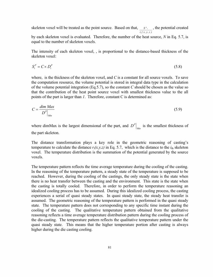
81

skeleton voxel will be treated as the point source. Based on that, )z,y,x(r

S

i

ip , the potential created

by each skeleton voxel is evaluated. Therefore, the number of the heat source, N in Eq. 5.7, is equal to the number of skeleton voxels.

The intensity of each skeleton voxel, , is proportional to the distance-based thickness of the skeleton voxel:

Pi

Pi DCS ×= (5.8)

where, is the thickness of the skeleton voxel, and C is a constant for all source voxels. To save the computation resource, the volume potential is stored in integral data type in the calculation of the volume potential integration (Eq.5.7), so the constant C should be chosen as the value so that the contribution of the heat point source voxel with smallest thickness value to the all points of the part is larger than 1. Therefore, constant C is determined as:

Min

PDMaxdimC = (5.9)

where dimMax is the largest dimensional of the part, and Min

PD is the smallest thickness of

the part skeleton.

The distance transformation plays a key role in the geometric reasoning of casting’s temperature to calculate the distance ri(x,y,z) in Eq. 5.7, which is the distance to the ith skeleton voxel. The temperature distribution is the summation of the potential generated by the source voxels.

The temperature pattern reflects the time average temperature during the cooling of the casting. In the reasoning of the temperature pattern, a steady state of the temperature is supposed to be reached. However, during the cooling of the castings, the only steady state is the state when there is no heat transfer between the casting and the environment. This state is the state when the casting is totally cooled. Therefore, in order to perform the temperature reasoning an idealized cooling process has to be assumed. During this idealized cooling process, the casting experiences a serial of quasi steady states. In quasi steady state, the steady heat transfer is assumed. The geometric reasoning of the temperature pattern is performed in the quasi steady state. The temperature pattern does not corresponding to any specific time instant during the cooling of the casting. The qualitative temperature pattern obtained from the qualitative reasoning reflects a time average temperature distribution pattern during the cooling process of the die-casting. The temperature pattern reflects the qualitative temperature pattern under the quasi steady state. This means that the higher temperature portion after casting is always higher during the die casting cooling.

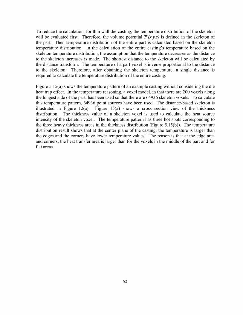
82

To reduce the calculation, for thin wall die-casting, the temperature distribution of the skeleton will be evaluated first. Therefore, the volume potential Tp(x,y,z) is defined in the skeleton of the part. Then temperature distribution of the entire part is calculated based on the skeleton temperature distribution. In the calculation of the entire casting’s temperature based on the skeleton temperature distribution, the assumption that the temperature decreases as the distance to the skeleton increases is made. The shortest distance to the skeleton will be calculated by the distance transform. The temperature of a part voxel is inverse proportional to the distance to the skeleton. Therefore, after obtaining the skeleton temperature, a single distance is required to calculate the temperature distribution of the entire casting.

Figure 5.15(a) shows the temperature pattern of an example casting without considering the die heat trap effect. In the temperature reasoning, a voxel model, in that there are 200 voxels along the longest side of the part, has been used so that there are 64936 skeleton voxels. To calculate this temperature pattern, 64936 point sources have been used. The distance-based skeleton is illustrated in Figure 12(a). Figure 15(a) shows a cross section view of the thickness distribution. The thickness value of a skeleton voxel is used to calculate the heat source intensity of the skeleton voxel. The temperature pattern has three hot spots corresponding to the three heavy thickness areas in the thickness distribution (Figure 5.15(b)). The temperature distribution result shows that at the center plane of the casting, the temperature is larger than the edges and the corners have lower temperature values. The reason is that at the edge area and corners, the heat transfer area is larger than for the voxels in the middle of the part and for flat areas.

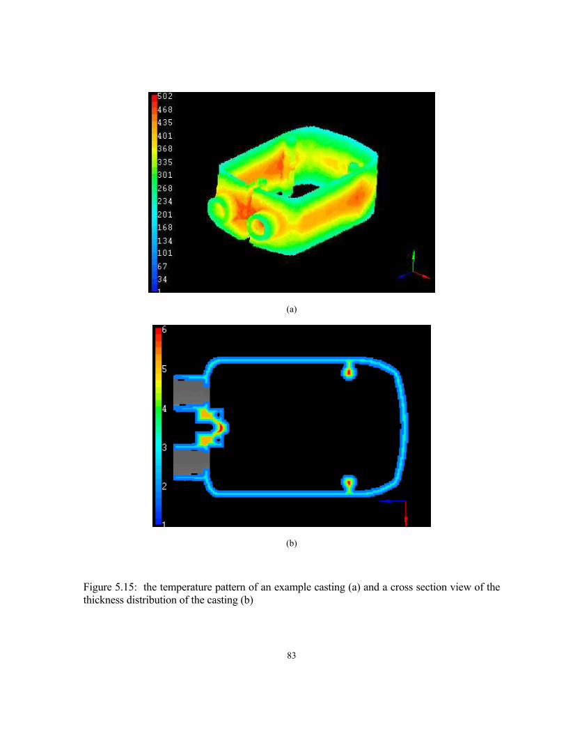
83

(a)

(b)

Figure 5.15: the temperature pattern of an example casting (a) and a cross section view of the thickness distribution of the casting (b)

84

Contribution of Heat Traps in De to the Temperature Distribution

Heat traps existing in the die can be heat sources that influence the temperature distribution in a casting. As shown in Figure 3.2, the heat traps are associated with the die skeleton. The thickness value of the die skeleton voxels is correlated to the temperature of the die voxels. The smaller the thickness value, the larger temperature it associates. Therefore, the source intensity of the heat source Sd

j is inverse proportional to the thickness of the die skeleton voxel. To convert the thickness value of die skeleton to the source intensity associated with the thickness value, a line interpolation function is used:

MinM

jMaxdj TT

TTS

−

−= (5.10)

where Tmax and Tmin are the maximal and minimal thickness value the die skeleton has, Tj is the jth die thickness value, and Sd

j is the source intensity of the heat source. The resulted intensity has been normalized into [0,1].

For the die casting process, the all heat energy comes from the liquid metal. Therefore, the heat sources in castings are dominant. Furthermore, how the heat traps influence the part temperature distribution is dependent on the die cooling and heat transfer boundary conditions between the die and casting, the die casting process and material related information. For a geometric reasoning method, it is difficult to scale the heat trap’s influence compared to the heat source in the casting. The effect of the heat traps can served to revise the temperature distribution based on the heat source in castings. Unfortunately, the scale factor W in Eq. 5.7 cannot be determined by the geometric reasoning only.

For each point source, the distance transformation is performed on the casting voxel model with the point source as the “source” voxel of the distance transformation. By mean of the distance transform, the distance distribution associated with the jth point heat source can be obtained and therefore, the potentials caused by the thermal equivalent point source are evaluated according to the Eq.5.7. Using the thickness values of the sub-skeletons as the part source intensity and Eq. 5.10 to evaluate the die heat source intensity, the summation of the potentials is obtained. For the current implementation, the weight factor F in Eq. 5.7 is an input variable dependent on how large the heat traps influence to the casting temperature. If F is set to zero, there is not the effect of the heat traps considered.

5.5 Plastic Distortion Pattern

The thin wall castings have been used for the analogy. Although considerable progress has been made in mathematically modeling the inelastic behavior, the qualitative approach can yield information of direct utility to the qualitative evaluation of plastic distortion. The postulated stress-strain relations are sufficiently simple so that it is possible to determine qualitatively how the ideal bodies they define behave under the qualitative temperature change.

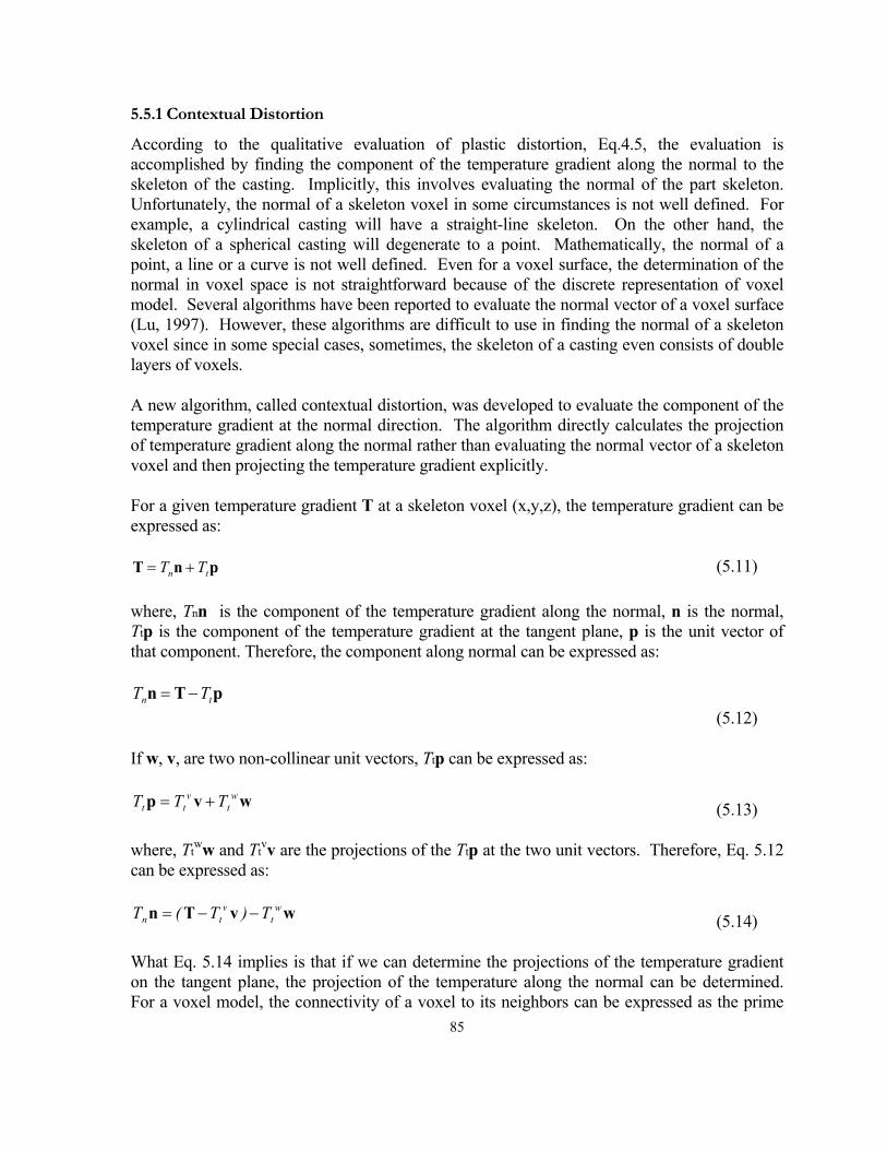
85

5.5.1 Contextual Distortion

According to the qualitative evaluation of plastic distortion, Eq.4.5, the evaluation is accomplished by finding the component of the temperature gradient along the normal to the skeleton of the casting. Implicitly, this involves evaluating the normal of the part skeleton. Unfortunately, the normal of a skeleton voxel in some circumstances is not well defined. For example, a cylindrical casting will have a straight-line skeleton. On the other hand, the skeleton of a spherical casting will degenerate to a point. Mathematically, the normal of a point, a line or a curve is not well defined. Even for a voxel surface, the determination of the normal in voxel space is not straightforward because of the discrete representation of voxel model. Several algorithms have been reported to evaluate the normal vector of a voxel surface (Lu, 1997). However, these algorithms are difficult to use in finding the normal of a skeleton voxel since in some special cases, sometimes, the skeleton of a casting even consists of double layers of voxels.

A new algorithm, called contextual distortion, was developed to evaluate the component of the temperature gradient at the normal direction. The algorithm directly calculates the projection of temperature gradient along the normal rather than evaluating the normal vector of a skeleton voxel and then projecting the temperature gradient explicitly.

For a given temperature gradient T at a skeleton voxel (x,y,z), the temperature gradient can be expressed as:

pnT tn TT += (5.11)

where, Tnn is the component of the temperature gradient along the normal, n is the normal, Ttp is the component of the temperature gradient at the tangent plane, p is the unit vector of that component. Therefore, the component along normal can be expressed as:

(5.12)

If w, v, are two non-collinear unit vectors, Ttp can be expressed as:

wvp wt

vtt TTT += (5.13)

where, Ttww and Tt

vv are the projections of the Ttp at the two unit vectors. Therefore, Eq. 5.12 can be expressed as:

wvTn wt

vtn T)T(T −−= (5.14)

What Eq. 5.14 implies is that if we can determine the projections of the temperature gradient on the tangent plane, the projection of the temperature along the normal can be determined. For a voxel model, the connectivity of a voxel to its neighbors can be expressed as the prime

pTn tn TT −=

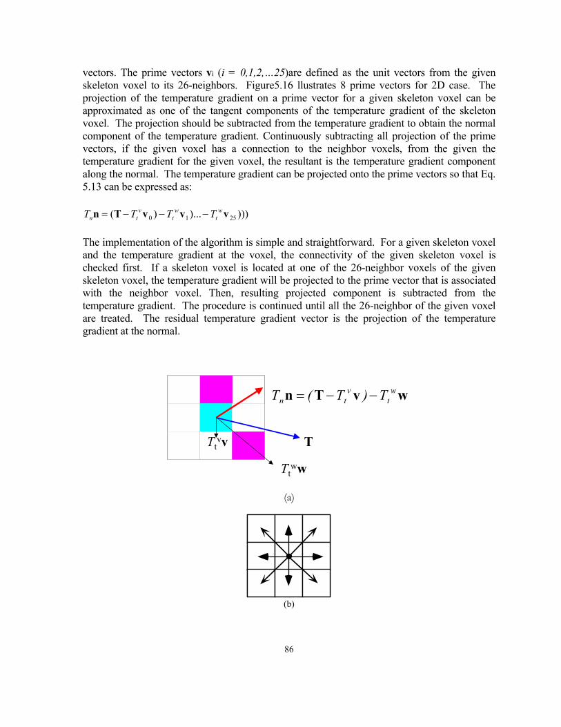
86

vectors. The prime vectors vi (i = 0,1,2,…25)are defined as the unit vectors from the given skeleton voxel to its 26-neighbors. Figure5.16 llustrates 8 prime vectors for 2D case. The projection of the temperature gradient on a prime vector for a given skeleton voxel can be approximated as one of the tangent components of the temperature gradient of the skeleton voxel. The projection should be subtracted from the temperature gradient to obtain the normal component of the temperature gradient. Continuously subtracting all projection of the prime vectors, if the given voxel has a connection to the neighbor voxels, from the given the temperature gradient for the given voxel, the resultant is the temperature gradient component along the normal. The temperature gradient can be projected onto the prime vectors so that Eq. 5.13 can be expressed as:

))))...)( 2510 vvvTn wt

wt

vtn TTTT −−−=

The implementation of the algorithm is simple and straightforward. For a given skeleton voxel and the temperature gradient at the voxel, the connectivity of the given skeleton voxel is checked first. If a skeleton voxel is located at one of the 26-neighbor voxels of the given skeleton voxel, the temperature gradient will be projected to the prime vector that is associated with the neighbor voxel. Then, resulting projected component is subtracted from the temperature gradient. The procedure is continued until all the 26-neighbor of the given voxel are treated. The residual temperature gradient vector is the projection of the temperature gradient at the normal.

wvTn wt

vtn T)T(T −−=

Ttww

TTtvv

(a)

(b)

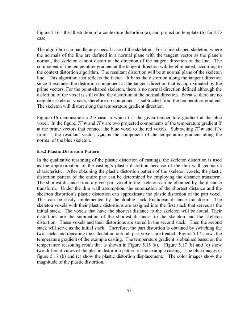
87

Figure 5.16: the Illustration of a contexture distortion (a), and projection template (b) for 2-D case

The algorithm can handle any special case of the skeleton. For a line-shaped skeleton, where the normals of the line are defined in a normal plane with the tangent vector as the plane’s normal, the skeleton cannot distort at the direction of the tangent direction of the line. The component of the temperature gradient at the tangent direction will be eliminated, according to the context distortion algorithm. The resultant distortion will be at normal plane of the skeleton line. This algorithm just reflects the factor. It bans the distortion along the tangent direction since it excludes the distortion component at the tangent direction that is approximated by the prime vectors. For the point-shaped skeleton, there is no normal direction defined although the distortion of the voxel is still called the distortion at the normal direction. Because there are no neighbor skeleton voxels, therefore no component is subtracted from the temperature gradient. The skeleton will distort along the temperature gradient direction.

Figure5.16 demonstrate a 2D case in which t is the given temperature gradient at the blue voxel. In the figure, Tt

ww and Ttvv are two projected components of the temperature gradient T

at the prime vectors that connect the blue voxel to the red voxels. Subtracting Ttww and Tt

vv from T, the resultant vector, Tnn, is the component of the temperature gradient along the normal of the blue skeleton.

5.5.2 Plastic Distortion Pattern

In the qualitative reasoning of the plastic distortion of castings, the skeleton distortion is used as the approximation of the casting’s plastic distortion because of the thin wall geometric characteristic. After obtaining the plastic distortion pattern of the skeleton voxels, the plastic distortion pattern of the entire part can be determined by employing the distance transform. The shortest distance from a given part voxel to the skeleton can be obtained by the distance transform. Under the thin wall assumption, the summation of the shortest distance and the skeleton distortion’s plastic distortion can approximate the plastic distortion of the part voxel. This can be easily implemented by the double-stack Euclidean distance transform. The skeleton voxels with their plastic distortions are assigned into the first stack that serves as the initial stack. The voxels that have the shortest distance to the skeleton will be found. Their distortions are the summation of the shortest distances to the skeleton and the skeleton distortion. These voxels and their distortions are stored in the second stack. Then the second stack will serve as the initial stack. Therefore, the part distortion is obtained by switching the two stacks and repeating the calculation until all part voxels are treated. Figure 5.17 shows the temperature gradient of the example casting. The temperature gradient is obtained based on the temperature reasoning result that is shown in Figure 5.15 (a). Figure 5.17 (b) and (c) show two different views of the plastic distortion pattern of the example casting. The blue images in figure 5.17 (b) and (c) show the plastic distortion displacement. The color images show the magnitude of the plastic distortion.

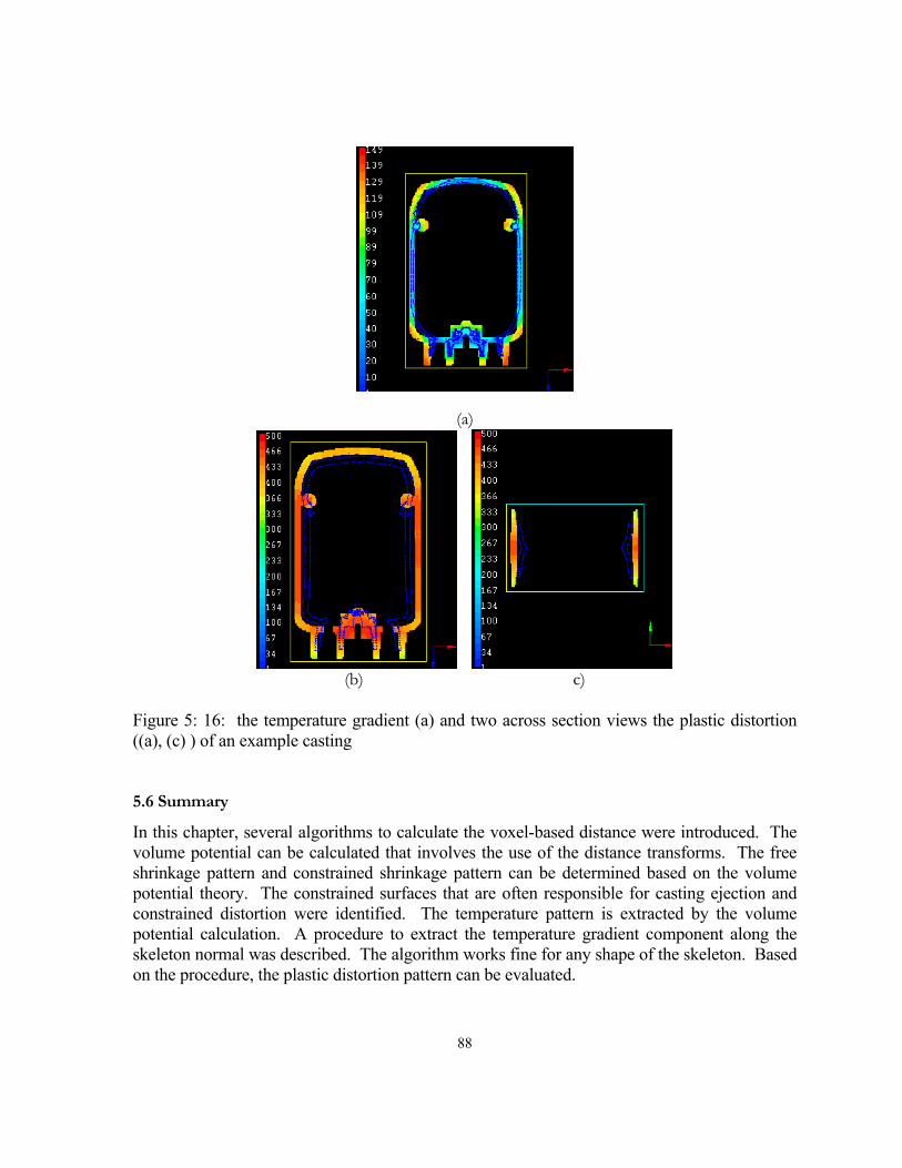
88

(a)

(b) c)

Figure 5: 16: the temperature gradient (a) and two across section views the plastic distortion ((a), (c) ) of an example casting

5.6 Summary

In this chapter, several algorithms to calculate the voxel-based distance were introduced. The volume potential can be calculated that involves the use of the distance transforms. The free shrinkage pattern and constrained shrinkage pattern can be determined based on the volume potential theory. The constrained surfaces that are often responsible for casting ejection and constrained distortion were identified. The temperature pattern is extracted by the volume potential calculation. A procedure to extract the temperature gradient component along the skeleton normal was described. The algorithm works fine for any shape of the skeleton. Based on the procedure, the plastic distortion pattern can be evaluated.

89

6. THE EVALUATION OF EJECTABILITY OF CASTING BY GEOMETRIC REASONING

6.1 Introduction

Ejectability is a measurement of a casting design considering the influence of the casting distortion effects on the ejection operation. The distortion-induced interaction between casting and die is a critical factor to determine ejector pin locations and the orientation of casting to the die. For some casting features where normal shrinkage cannot take place due to resistance of the die wall, non-uniform shrinkage will be developed (Housner,1966). Since normal shrinkage cannot take place when constrained surfaces are present, equivalent internal stress develops as the casting cools from its solidification temperature to its ejection temperature. This results in an ejection load on the constrained surfaces. This ejection load creates an ejection resistance during the ejection operation of the die casting process. With the help of the ejector pins, the ejection load acting on the constrained surfaces of castings will be released when the casting is pushed off the ejector die surface. The position, number and size of ejector pins must be carefully planned to overcome the resistance to ejection. The geometric characteristics and the ejection load of castings play important roles in determining the ejector pin’s number, location, size, shape, and distribution (Herman,1985).

The ejection load also influences the orientation of the cavity with respect to the parting surfaces of the die. The primary consideration is to place the constrained surfaces that have higher ejection load in the ejector die. Generally, this requires that the casting shrink onto the constrained surfaces. As the die opens, the constrained surfaces will stick to these ejector die surfaces and be pulled out of the cover die cavity. As the die is opened, the ejector pins are moved forward to push the casting out of the ejector die half.

This chapter discusses a geometric reasoning approach to qualitatively evaluate a casting’s ejectability. In previous chapters, the geometric reasoning approaches have been introduced to qualitatively evaluate casting distortion. With these qualitative reasonings, the casting’s free shrinkage pattern can be evaluated and constrained surfaces can be extracted. Following the steps of our previous research about casting distortion, the ejectability of castings can be qualitatively evaluated by defining and evaluating several functions including the effective relative ejection force rating of each ejector pin, ejection moment, ejection pattern, the ratio of the ejection load on ejector die to that on cover die. The information can help die designers to evaluate their ejector pin layouts and make design decision about locating ejector pins and orienting the part in the die. Qualitative reasoning requires significantly less time than numerical simulation and can be used with much less information available making it a good candidate for preliminary screening and design decision making.

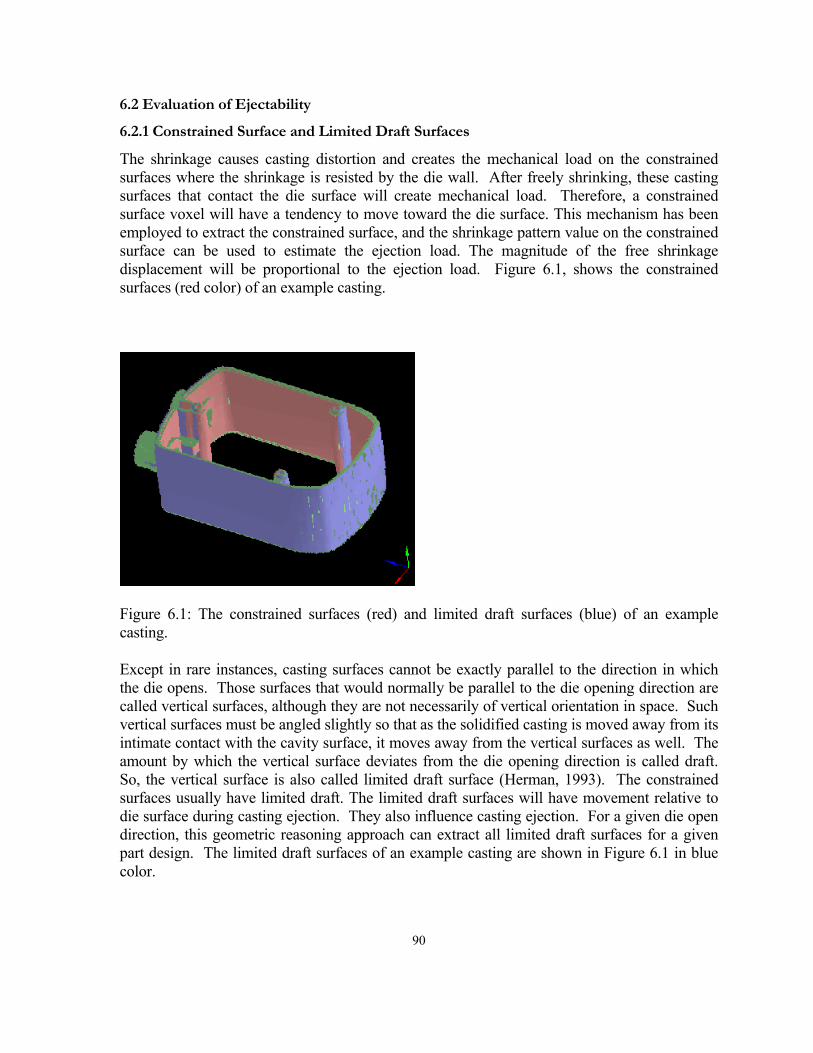
90

6.2 Evaluation of Ejectability

6.2.1 Constrained Surface and Limited Draft Surfaces

The shrinkage causes casting distortion and creates the mechanical load on the constrained surfaces where the shrinkage is resisted by the die wall. After freely shrinking, these casting surfaces that contact the die surface will create mechanical load. Therefore, a constrained surface voxel will have a tendency to move toward the die surface. This mechanism has been employed to extract the constrained surface, and the shrinkage pattern value on the constrained surface can be used to estimate the ejection load. The magnitude of the free shrinkage displacement will be proportional to the ejection load. Figure 6.1, shows the constrained surfaces (red color) of an example casting.

Figure 6.1: The constrained surfaces (red) and limited draft surfaces (blue) of an example casting.

Except in rare instances, casting surfaces cannot be exactly parallel to the direction in which the die opens. Those surfaces that would normally be parallel to the die opening direction are called vertical surfaces, although they are not necessarily of vertical orientation in space. Such vertical surfaces must be angled slightly so that as the solidified casting is moved away from its intimate contact with the cavity surface, it moves away from the vertical surfaces as well. The amount by which the vertical surface deviates from the die opening direction is called draft. So, the vertical surface is also called limited draft surface (Herman, 1993). The constrained surfaces usually have limited draft. The limited draft surfaces will have movement relative to die surface during casting ejection. They also influence casting ejection. For a given die open direction, this geometric reasoning approach can extract all limited draft surfaces for a given part design. The limited draft surfaces of an example casting are shown in Figure 6.1 in blue color.

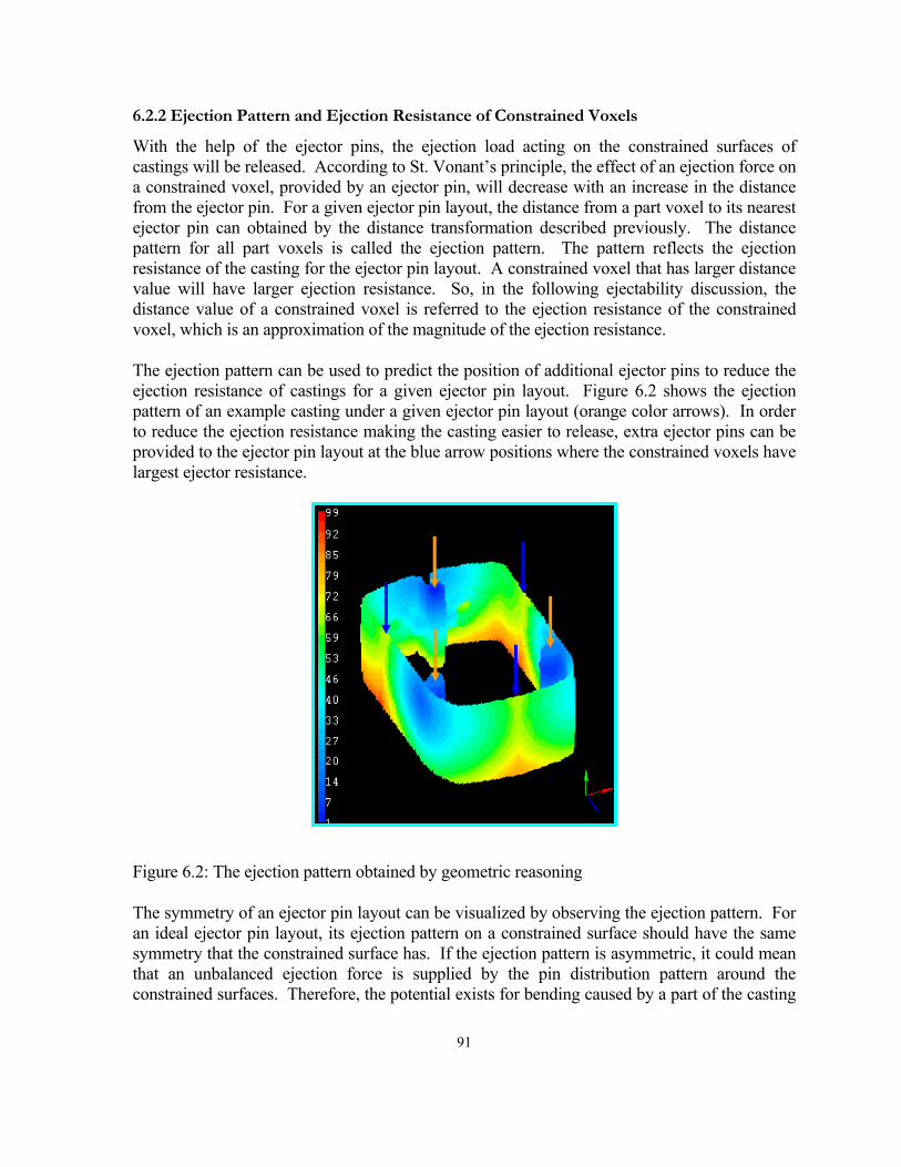
91

6.2.2 Ejection Pattern and Ejection Resistance of Constrained Voxels

With the help of the ejector pins, the ejection load acting on the constrained surfaces of castings will be released. According to St. Vonant’s principle, the effect of an ejection force on a constrained voxel, provided by an ejector pin, will decrease with an increase in the distance from the ejector pin. For a given ejector pin layout, the distance from a part voxel to its nearest ejector pin can obtained by the distance transformation described previously. The distance pattern for all part voxels is called the ejection pattern. The pattern reflects the ejection resistance of the casting for the ejector pin layout. A constrained voxel that has larger distance value will have larger ejection resistance. So, in the following ejectability discussion, the distance value of a constrained voxel is referred to the ejection resistance of the constrained voxel, which is an approximation of the magnitude of the ejection resistance.

The ejection pattern can be used to predict the position of additional ejector pins to reduce the ejection resistance of castings for a given ejector pin layout. Figure 6.2 shows the ejection pattern of an example casting under a given ejector pin layout (orange color arrows). In order to reduce the ejection resistance making the casting easier to release, extra ejector pins can be provided to the ejector pin layout at the blue arrow positions where the constrained voxels have largest ejector resistance.

Figure 6.2: The ejection pattern obtained by geometric reasoning

The symmetry of an ejector pin layout can be visualized by observing the ejection pattern. For an ideal ejector pin layout, its ejection pattern on a constrained surface should have the same symmetry that the constrained surface has. If the ejection pattern is asymmetric, it could mean that an unbalanced ejection force is supplied by the pin distribution pattern around the constrained surfaces. Therefore, the potential exists for bending caused by a part of the casting

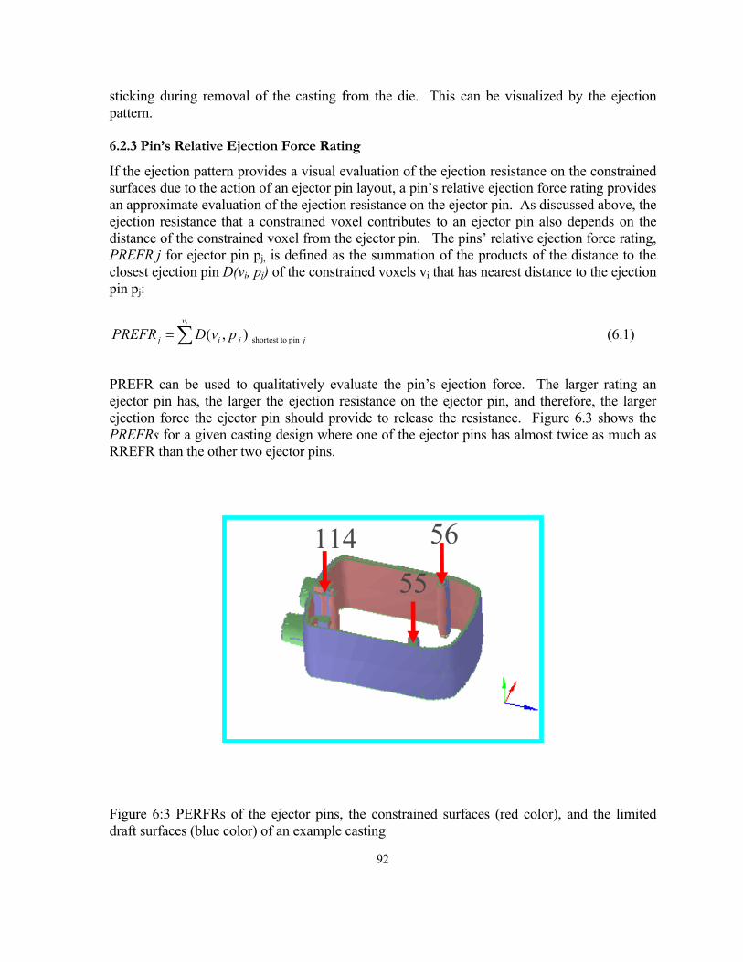
92

sticking during removal of the casting from the die. This can be visualized by the ejection pattern.

6.2.3 Pin’s Relative Ejection Force Rating

If the ejection pattern provides a visual evaluation of the ejection resistance on the constrained surfaces due to the action of an ejector pin layout, a pin’s relative ejection force rating provides an approximate evaluation of the ejection resistance on the ejector pin. As discussed above, the ejection resistance that a constrained voxel contributes to an ejector pin also depends on the distance of the constrained voxel from the ejector pin. The pins’ relative ejection force rating, PREFR j for ejector pin pj, is defined as the summation of the products of the distance to the closest ejection pin D(vi, pj) of the constrained voxels vi that has nearest distance to the ejection pin pj:

∑=iv

jjij pvDPREFR pin oshortest t),( (6.1)

PREFR can be used to qualitatively evaluate the pin’s ejection force. The larger rating an ejector pin has, the larger the ejection resistance on the ejector pin, and therefore, the larger ejection force the ejector pin should provide to release the resistance. Figure 6.3 shows the PREFRs for a given casting design where one of the ejector pins has almost twice as much as RREFR than the other two ejector pins.

56

55114

Figure 6:3 PERFRs of the ejector pins, the constrained surfaces (red color), and the limited draft surfaces (blue color) of an example casting

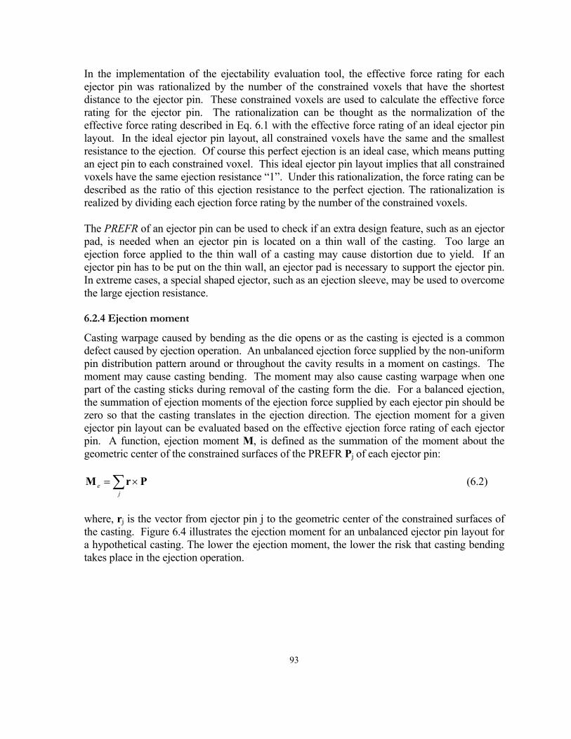
93

In the implementation of the ejectability evaluation tool, the effective force rating for each ejector pin was rationalized by the number of the constrained voxels that have the shortest distance to the ejector pin. These constrained voxels are used to calculate the effective force rating for the ejector pin. The rationalization can be thought as the normalization of the effective force rating described in Eq. 6.1 with the effective force rating of an ideal ejector pin layout. In the ideal ejector pin layout, all constrained voxels have the same and the smallest resistance to the ejection. Of course this perfect ejection is an ideal case, which means putting an eject pin to each constrained voxel. This ideal ejector pin layout implies that all constrained voxels have the same ejection resistance “1”. Under this rationalization, the force rating can be described as the ratio of this ejection resistance to the perfect ejection. The rationalization is realized by dividing each ejection force rating by the number of the constrained voxels.

The PREFR of an ejector pin can be used to check if an extra design feature, such as an ejector pad, is needed when an ejector pin is located on a thin wall of the casting. Too large an ejection force applied to the thin wall of a casting may cause distortion due to yield. If an ejector pin has to be put on the thin wall, an ejector pad is necessary to support the ejector pin. In extreme cases, a special shaped ejector, such as an ejection sleeve, may be used to overcome the large ejection resistance.

6.2.4 Ejection moment

Casting warpage caused by bending as the die opens or as the casting is ejected is a common defect caused by ejection operation. An unbalanced ejection force supplied by the non-uniform pin distribution pattern around or throughout the cavity results in a moment on castings. The moment may cause casting bending. The moment may also cause casting warpage when one part of the casting sticks during removal of the casting form the die. For a balanced ejection, the summation of ejection moments of the ejection force supplied by each ejector pin should be zero so that the casting translates in the ejection direction. The ejection moment for a given ejector pin layout can be evaluated based on the effective ejection force rating of each ejector pin. A function, ejection moment M, is defined as the summation of the moment about the geometric center of the constrained surfaces of the PREFR Pj of each ejector pin:

PrM ×=∑j

e (6.2)

where, rj is the vector from ejector pin j to the geometric center of the constrained surfaces of the casting. Figure 6.4 illustrates the ejection moment for an unbalanced ejector pin layout for a hypothetical casting. The lower the ejection moment, the lower the risk that casting bending takes place in the ejection operation.

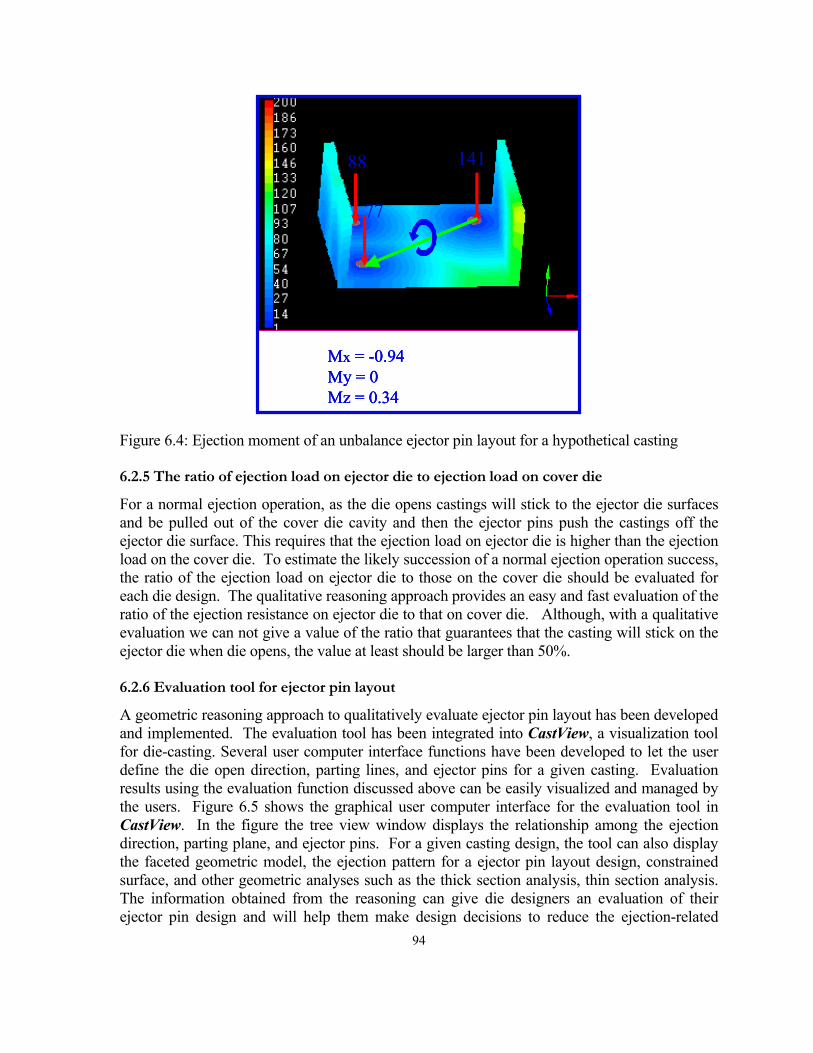
94

88

77

141

Mx = -0.94My = 0Mz = 0.34

88

77

141

Mx = -0.94My = 0Mz = 0.34

88

77

141

Mx = -0.94My = 0Mz = 0.34

Figure 6.4: Ejection moment of an unbalance ejector pin layout for a hypothetical casting

6.2.5 The ratio of ejection load on ejector die to ejection load on cover die

For a normal ejection operation, as the die opens castings will stick to the ejector die surfaces and be pulled out of the cover die cavity and then the ejector pins push the castings off the ejector die surface. This requires that the ejection load on ejector die is higher than the ejection load on the cover die. To estimate the likely succession of a normal ejection operation success, the ratio of the ejection load on ejector die to those on the cover die should be evaluated for each die design. The qualitative reasoning approach provides an easy and fast evaluation of the ratio of the ejection resistance on ejector die to that on cover die. Although, with a qualitative evaluation we can not give a value of the ratio that guarantees that the casting will stick on the ejector die when die opens, the value at least should be larger than 50%.

6.2.6 Evaluation tool for ejector pin layout

A geometric reasoning approach to qualitatively evaluate ejector pin layout has been developed and implemented. The evaluation tool has been integrated into CastView, a visualization tool for die-casting. Several user computer interface functions have been developed to let the user define the die open direction, parting lines, and ejector pins for a given casting. Evaluation results using the evaluation function discussed above can be easily visualized and managed by the users. Figure 6.5 shows the graphical user computer interface for the evaluation tool in CastView. In the figure the tree view window displays the relationship among the ejection direction, parting plane, and ejector pins. For a given casting design, the tool can also display the faceted geometric model, the ejection pattern for a ejector pin layout design, constrained surface, and other geometric analyses such as the thick section analysis, thin section analysis. The information obtained from the reasoning can give die designers an evaluation of their ejector pin design and will help them make design decisions to reduce the ejection-related

95

defects. The information can also help die designers locate ejector pins and orient the part in the die to perform a deformation free, fast, and smooth ejection operation.

6.3 Summary

Casting ejectability can be qualitatively evaluated by geometric reasoning. The geometric reasoning can extract the constrained surfaces and calculate the ejectability evaluation functions easily and efficiently. The geometric reasoning is suitable at the early design stage where the detailed material and process data are not well defined. Especially, die design engineers can take advantage of this tool when there are many alternative designs to evaluate. By using this tool, they can quickly sort through many what-ifs and select a good alternative using less product development time and cost than would otherwise be possible.

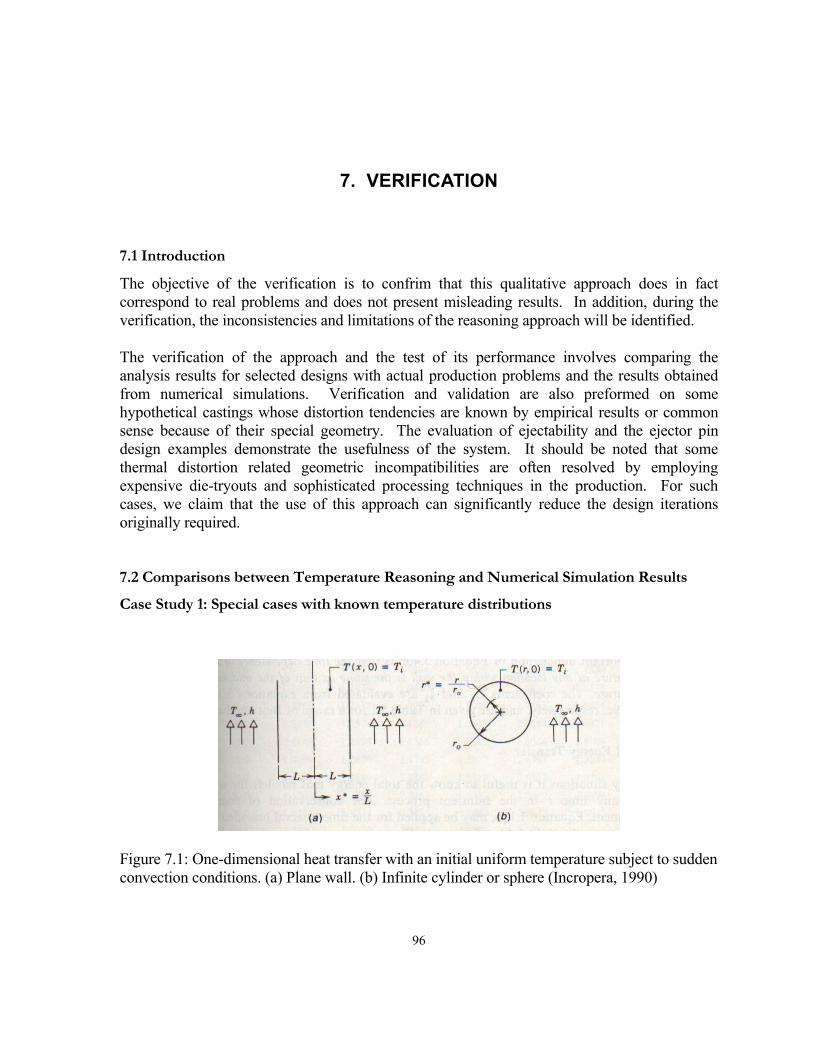
96

7. VERIFICATION

7.1 Introduction

The objective of the verification is to confrim that this qualitative approach does in fact correspond to real problems and does not present misleading results. In addition, during the verification, the inconsistencies and limitations of the reasoning approach will be identified.

The verification of the approach and the test of its performance involves comparing the analysis results for selected designs with actual production problems and the results obtained from numerical simulations. Verification and validation are also preformed on some hypothetical castings whose distortion tendencies are known by empirical results or common sense because of their special geometry. The evaluation of ejectability and the ejector pin design examples demonstrate the usefulness of the system. It should be noted that some thermal distortion related geometric incompatibilities are often resolved by employing expensive die-tryouts and sophisticated processing techniques in the production. For such cases, we claim that the use of this approach can significantly reduce the design iterations originally required.

7.2 Comparisons between Temperature Reasoning and Numerical Simulation Results

Case Study 1: Special cases with known temperature distributions

Figure 7.1: One-dimensional heat transfer with an initial uniform temperature subject to sudden convection conditions. (a) Plane wall. (b) Infinite cylinder or sphere (Incropera, 1990)

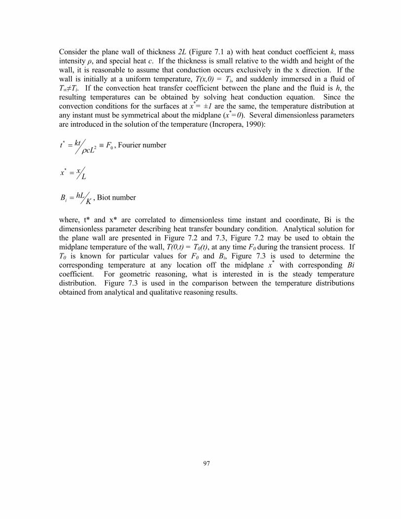
97

Consider the plane wall of thickness 2L (Figure 7.1 a) with heat conduct coefficient k, mass intensity ρ, and special heat c. If the thickness is small relative to the width and height of the wall, it is reasonable to assume that conduction occurs exclusively in the x direction. If the wall is initially at a uniform temperature, T(x,0) = Ti, and suddenly immersed in a fluid of T∞≠Ti. If the convection heat transfer coefficient between the plane and the fluid is h, the resulting temperatures can be obtained by solving heat conduction equation. Since the convection conditions for the surfaces at x*= ±1 are the same, the temperature distribution at any instant must be symmetrical about the midplane (x*=0). Several dimensionless parameters are introduced in the solution of the temperature (Incropera, 1990):

02 FcLktt* ≡= ρ , Fourier number

Lxx* =

KhLBi = , Biot number

where, t* and x* are correlated to dimensionless time instant and coordinate, Bi is the dimensionless parameter describing heat transfer boundary condition. Analytical solution for the plane wall are presented in Figure 7.2 and 7.3, Figure 7.2 may be used to obtain the midplane temperature of the wall, T(0,t) = T0(t), at any time F0 during the transient process. If T0 is known for particular values for F0 and Bi, Figure 7.3 is used to determine the corresponding temperature at any location off the midplane x* with corresponding Bi coefficient. For geometric reasoning, what is interested in is the steady temperature distribution. Figure 7.3 is used in the comparison between the temperature distributions obtained from analytical and qualitative reasoning results.

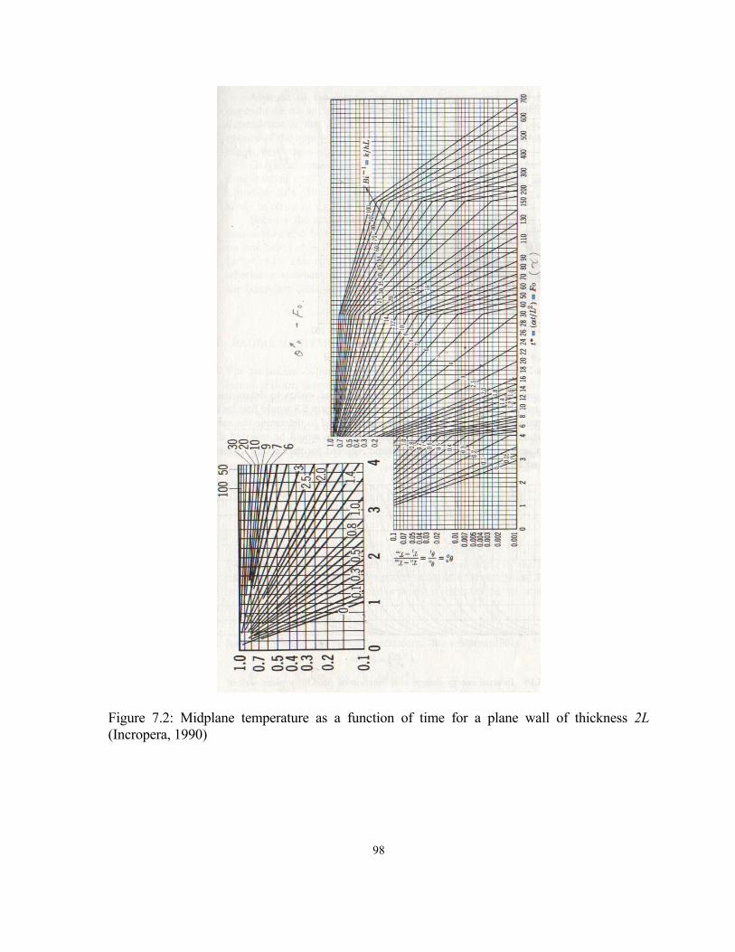
98

Figure 7.2: Midplane temperature as a function of time for a plane wall of thickness 2L (Incropera, 1990)

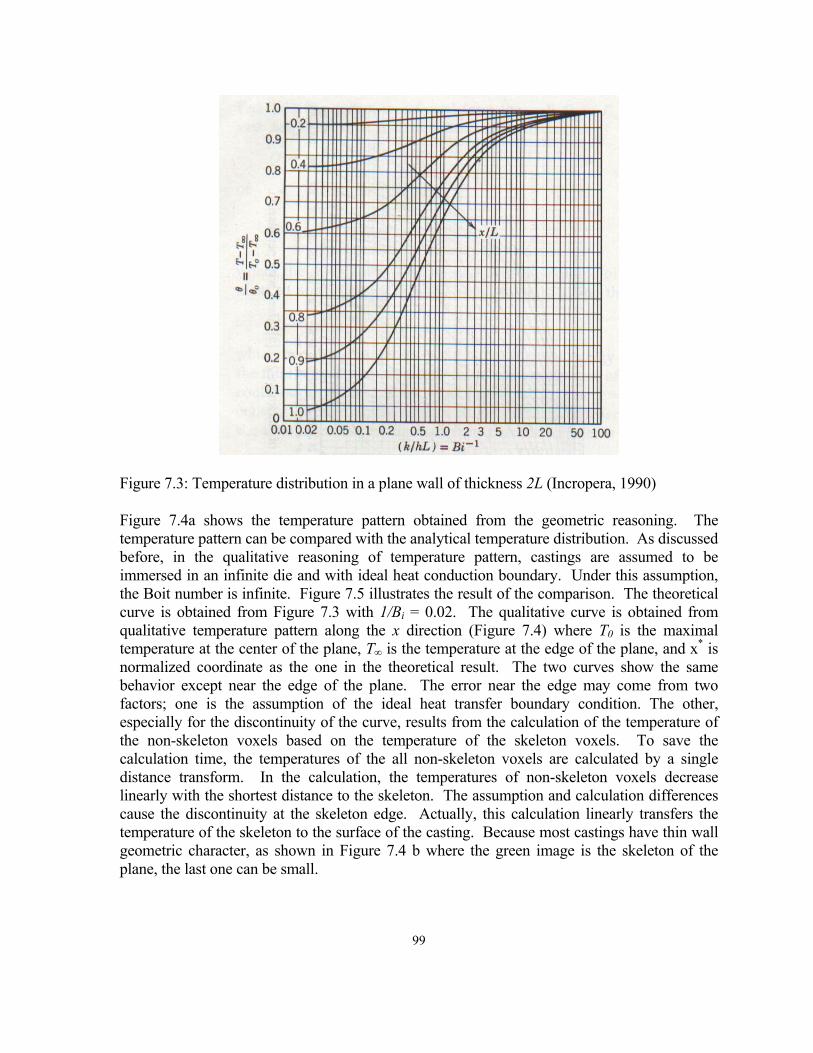
99

Figure 7.3: Temperature distribution in a plane wall of thickness 2L (Incropera, 1990)

Figure 7.4a shows the temperature pattern obtained from the geometric reasoning. The temperature pattern can be compared with the analytical temperature distribution. As discussed before, in the qualitative reasoning of temperature pattern, castings are assumed to be immersed in an infinite die and with ideal heat conduction boundary. Under this assumption, the Boit number is infinite. Figure 7.5 illustrates the result of the comparison. The theoretical curve is obtained from Figure 7.3 with 1/Bi = 0.02. The qualitative curve is obtained from qualitative temperature pattern along the x direction (Figure 7.4) where T0 is the maximal temperature at the center of the plane, T∞ is the temperature at the edge of the plane, and x* is normalized coordinate as the one in the theoretical result. The two curves show the same behavior except near the edge of the plane. The error near the edge may come from two factors; one is the assumption of the ideal heat transfer boundary condition. The other, especially for the discontinuity of the curve, results from the calculation of the temperature of the non-skeleton voxels based on the temperature of the skeleton voxels. To save the calculation time, the temperatures of the all non-skeleton voxels are calculated by a single distance transform. In the calculation, the temperatures of non-skeleton voxels decrease linearly with the shortest distance to the skeleton. The assumption and calculation differences cause the discontinuity at the skeleton edge. Actually, this calculation linearly transfers the temperature of the skeleton to the surface of the casting. Because most castings have thin wall geometric character, as shown in Figure 7.4 b where the green image is the skeleton of the plane, the last one can be small.

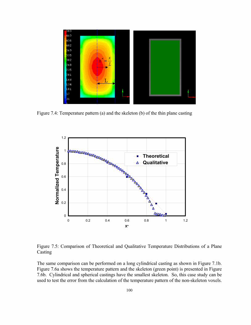
100

Figure 7.4: Temperature pattern (a) and the skeleton (b) of the thin plane casting

0

0.2

0.4

0.6

0.8

1

1.2

0 0.2 0.4 0.6 0.8 1 1.2

X*

Nor

mal

ized

Tem

pera

ture

TheoreticalQualitative

Figure 7.5: Comparison of Theoretical and Qualitative Temperature Distributions of a Plane Casting

The same comparison can be performed on a long cylindrical casting as shown in Figure 7.1b. Figure 7.6a shows the temperature pattern and the skeleton (green point) is presented in Figure 7.6b. Cylindrical and spherical castings have the smallest skeleton. So, this case study can be used to test the error from the calculation of the temperature pattern of the non-skeleton voxels.

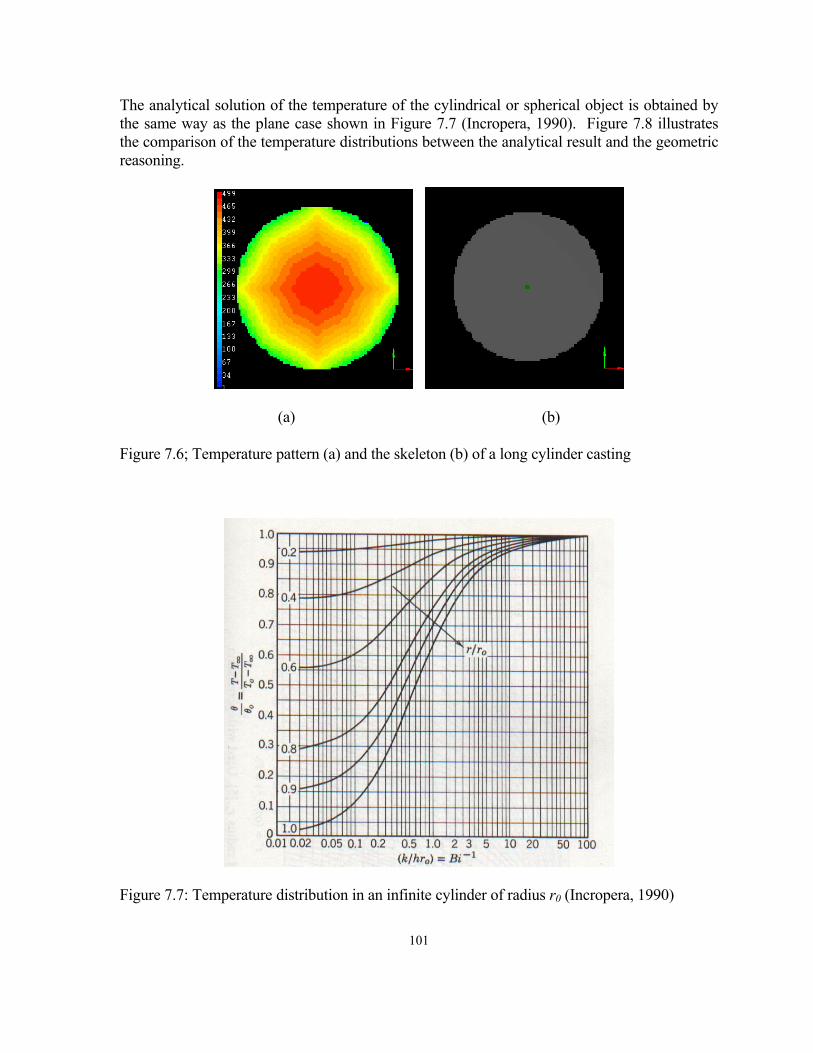
101

The analytical solution of the temperature of the cylindrical or spherical object is obtained by the same way as the plane case shown in Figure 7.7 (Incropera, 1990). Figure 7.8 illustrates the comparison of the temperature distributions between the analytical result and the geometric reasoning.

(a) (b)

Figure 7.6; Temperature pattern (a) and the skeleton (b) of a long cylinder casting

Figure 7.7: Temperature distribution in an infinite cylinder of radius r0 (Incropera, 1990)

102

0

0.2

0.4

0.6

0.8

1

1.2

0 0.2 0.4 0.6 0.8 1 1.2

X*

Nor

mal

ized

Tem

pera

ture

QualitativeTheoretical

Figure 7.8: Comparison of Theoretical and Qualitative Temperature Distributions of a cylindrical Casting

A long cylindrical casting is the extreme case for the qualitative reasoning in that its skeleton is a line. The qualitative reasoning obtains the temperature pattern of the skeleton, the single line, first. Then a distance transformation is employed to calculate the temperature of the non-skeleton voxels. The temperature pattern shows strong direction dependence. The direction dependence is caused by the accumulation calculation error when skeleton temperature is transferred to the surface of the cylinder. The integral data type has been used to store temperature value. The around error will take place for each step of the distance transformation calculation. The accumulation of the error causes the direction dependent temperature pattern. For the regular distance transformation, such as the thickness calculation, volume potential calculation, and the ejectability pattern calculation, the around error just takes place once when the norm of vector distance is calculated. The pattern obtained is non-direction dependent. For thin wall castings, the effect is quite week since the number of the steps is small.

In summery, in spite of some error in the calculation of the temperature of the non-skeleton voxels, the temperature patterns obtained from the geometric reasoning in this two special cases are qualitatively compatible with the temperature distributions obtained from analytical solution.

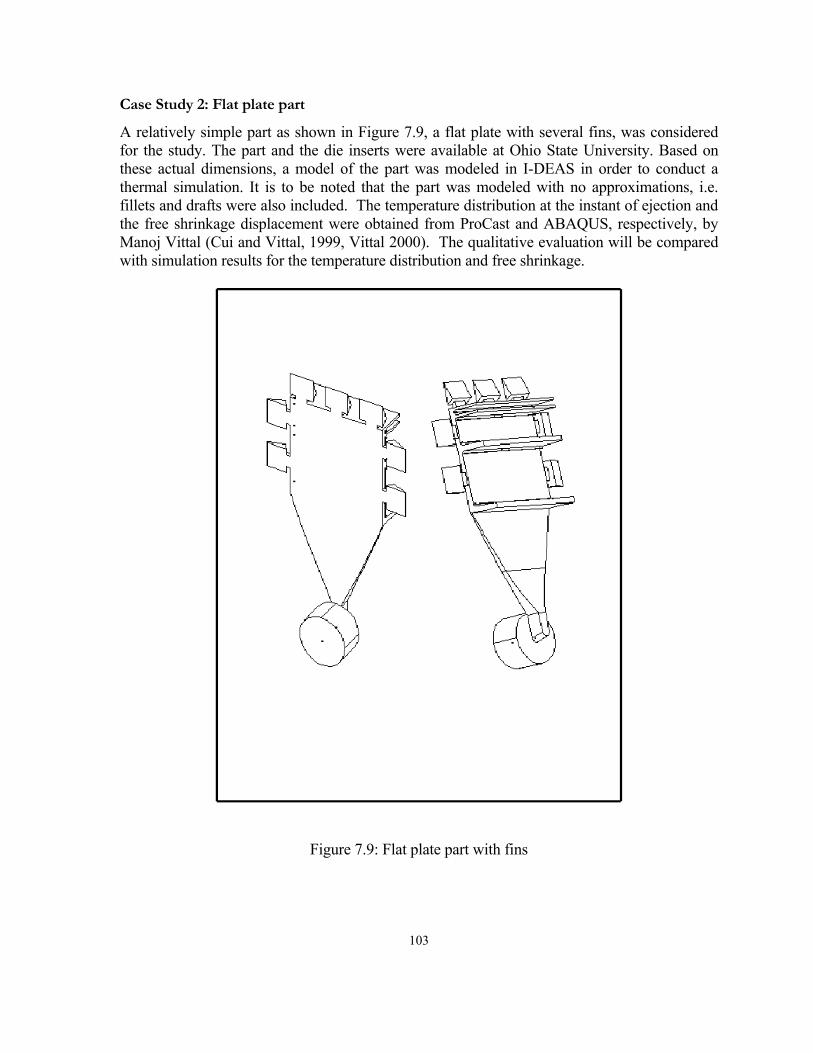
103

Case Study 2: Flat plate part

A relatively simple part as shown in Figure 7.9, a flat plate with several fins, was considered for the study. The part and the die inserts were available at Ohio State University. Based on these actual dimensions, a model of the part was modeled in I-DEAS in order to conduct a thermal simulation. It is to be noted that the part was modeled with no approximations, i.e. fillets and drafts were also included. The temperature distribution at the instant of ejection and the free shrinkage displacement were obtained from ProCast and ABAQUS, respectively, by Manoj Vittal (Cui and Vittal, 1999, Vittal 2000). The qualitative evaluation will be compared with simulation results for the temperature distribution and free shrinkage.

Figure 7.9: Flat plate part with fins

104

Comparison of Temperature Distributions

A thermal simulation was run in ProCast using the solid mesh generated in I-DEAS.The initial temperature of the part was assumed to be 670 deg C (1230 deg F) and that of the inserts 80 deg C. The material used for the inserts is H13 and that for the casting is the aluminum alloy A380. The temperature distribution of the casting (Figure 7.10 a) of the casting was obtained as results of the thermal simulation. The maximum temperature in the casting at the end of the cycle, i.e. at t = 45 seconds was observed to be around 225 °C. However, this was a one-cycle simulation, and therefore does not represent steady-state condition.

(a)

(b)

Figure 7.10: Temperature distributions obtained from Numerical simulation (a) and temperature reasoning (b)

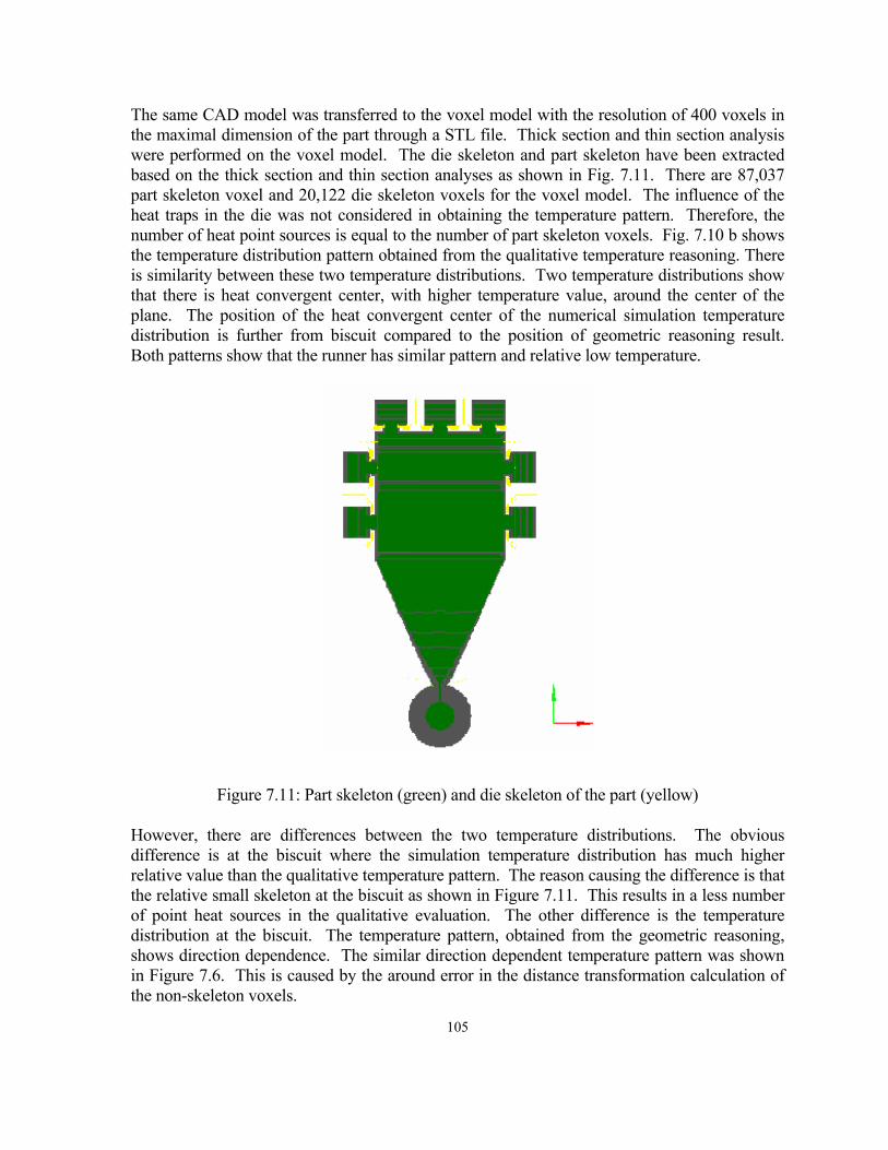
105

The same CAD model was transferred to the voxel model with the resolution of 400 voxels in the maximal dimension of the part through a STL file. Thick section and thin section analysis were performed on the voxel model. The die skeleton and part skeleton have been extracted based on the thick section and thin section analyses as shown in Fig. 7.11. There are 87,037 part skeleton voxel and 20,122 die skeleton voxels for the voxel model. The influence of the heat traps in the die was not considered in obtaining the temperature pattern. Therefore, the number of heat point sources is equal to the number of part skeleton voxels. Fig. 7.10 b shows the temperature distribution pattern obtained from the qualitative temperature reasoning. There is similarity between these two temperature distributions. Two temperature distributions show that there is heat convergent center, with higher temperature value, around the center of the plane. The position of the heat convergent center of the numerical simulation temperature distribution is further from biscuit compared to the position of geometric reasoning result. Both patterns show that the runner has similar pattern and relative low temperature.

Figure 7.11: Part skeleton (green) and die skeleton of the part (yellow)

However, there are differences between the two temperature distributions. The obvious difference is at the biscuit where the simulation temperature distribution has much higher relative value than the qualitative temperature pattern. The reason causing the difference is that the relative small skeleton at the biscuit as shown in Figure 7.11. This results in a less number of point heat sources in the qualitative evaluation. The other difference is the temperature distribution at the biscuit. The temperature pattern, obtained from the geometric reasoning, shows direction dependence. The similar direction dependent temperature pattern was shown in Figure 7.6. This is caused by the around error in the distance transformation calculation of the non-skeleton voxels.

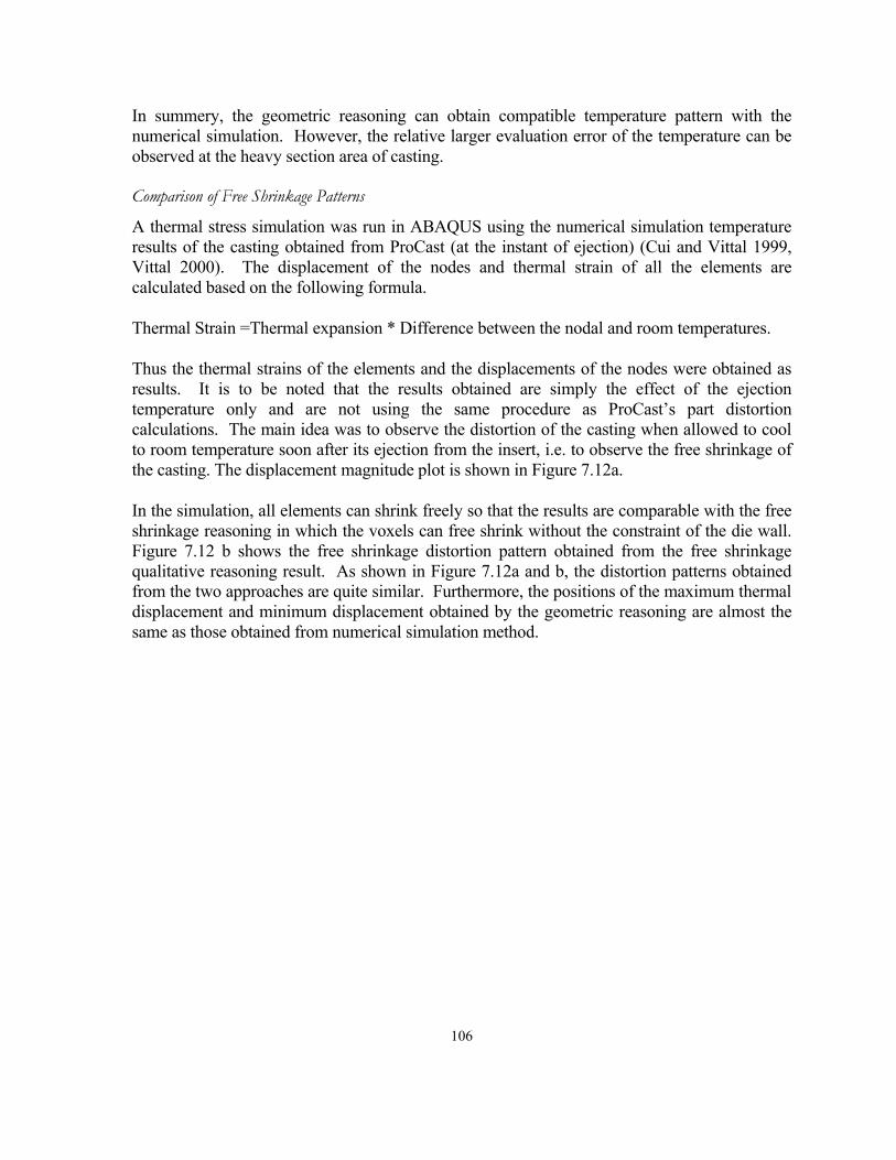
106

In summery, the geometric reasoning can obtain compatible temperature pattern with the numerical simulation. However, the relative larger evaluation error of the temperature can be observed at the heavy section area of casting.

Comparison of Free Shrinkage Patterns

A thermal stress simulation was run in ABAQUS using the numerical simulation temperature results of the casting obtained from ProCast (at the instant of ejection) (Cui and Vittal 1999, Vittal 2000). The displacement of the nodes and thermal strain of all the elements are calculated based on the following formula.

Thermal Strain =Thermal expansion * Difference between the nodal and room temperatures.

Thus the thermal strains of the elements and the displacements of the nodes were obtained as results. It is to be noted that the results obtained are simply the effect of the ejection temperature only and are not using the same procedure as ProCast’s part distortion calculations. The main idea was to observe the distortion of the casting when allowed to cool to room temperature soon after its ejection from the insert, i.e. to observe the free shrinkage of the casting. The displacement magnitude plot is shown in Figure 7.12a.

In the simulation, all elements can shrink freely so that the results are comparable with the free shrinkage reasoning in which the voxels can free shrink without the constraint of the die wall. Figure 7.12 b shows the free shrinkage distortion pattern obtained from the free shrinkage qualitative reasoning result. As shown in Figure 7.12a and b, the distortion patterns obtained from the two approaches are quite similar. Furthermore, the positions of the maximum thermal displacement and minimum displacement obtained by the geometric reasoning are almost the same as those obtained from numerical simulation method.

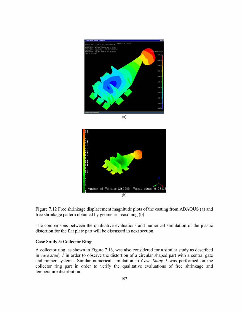
107

(a)

(b)

Figure 7.12 Free shrinkage displacement magnitude plots of the casting from ABAQUS (a) and free shrinkage pattern obtained by geometric reasoning (b)

The comparisons between the qualitative evaluations and numerical simulation of the plastic distortion for the flat plate part will be discussed in next section.

Case Study 3: Collector Ring

A collector ring, as shown in Figure 7.13, was also considered for a similar study as described in case study 1 in order to observe the distortion of a circular shaped part with a central gate and runner system. Similar numerical simulation to Case Study 1 was performed on the collector ring part in order to verify the qualitative evaluations of free shrinkage and temperature distribution.

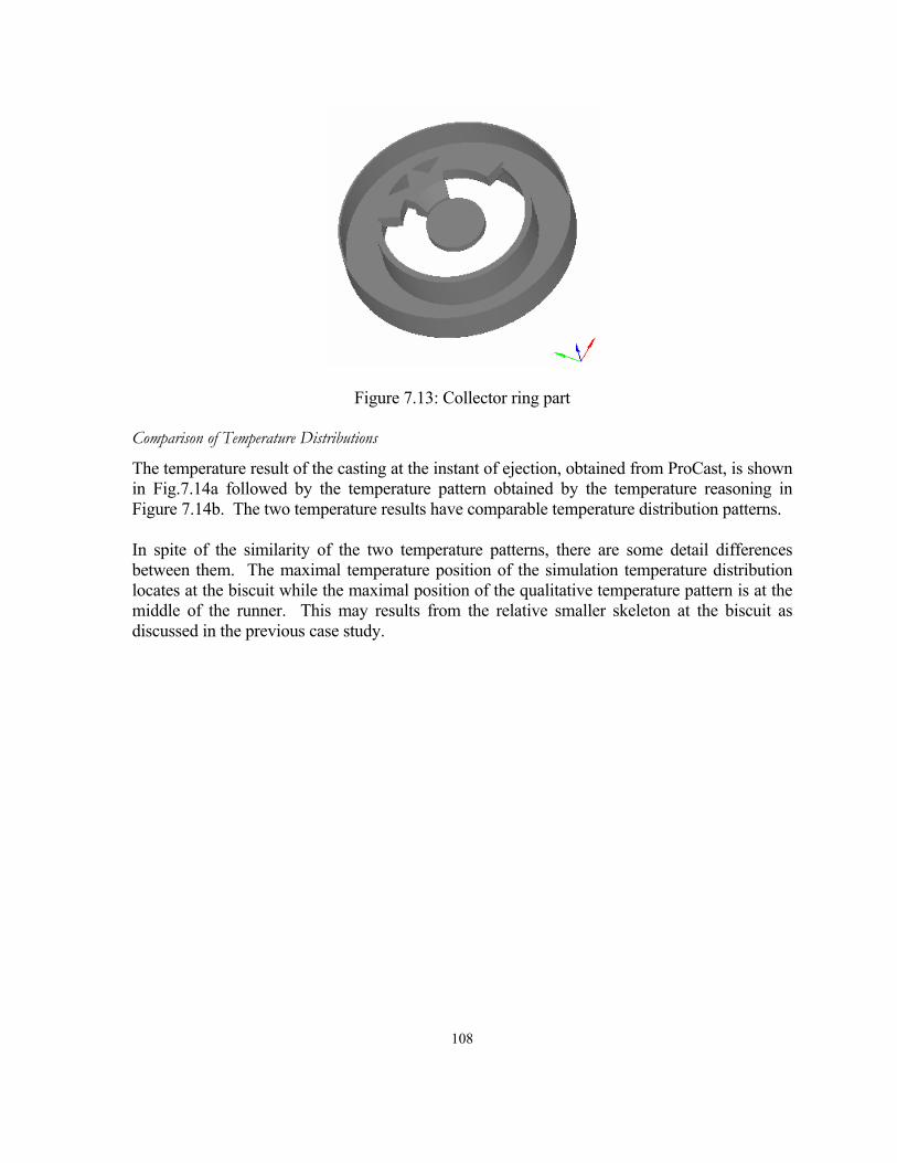
108

Figure 7.13: Collector ring part

Comparison of Temperature Distributions

The temperature result of the casting at the instant of ejection, obtained from ProCast, is shown in Fig.7.14a followed by the temperature pattern obtained by the temperature reasoning in Figure 7.14b. The two temperature results have comparable temperature distribution patterns.

In spite of the similarity of the two temperature patterns, there are some detail differences between them. The maximal temperature position of the simulation temperature distribution locates at the biscuit while the maximal position of the qualitative temperature pattern is at the middle of the runner. This may results from the relative smaller skeleton at the biscuit as discussed in the previous case study.

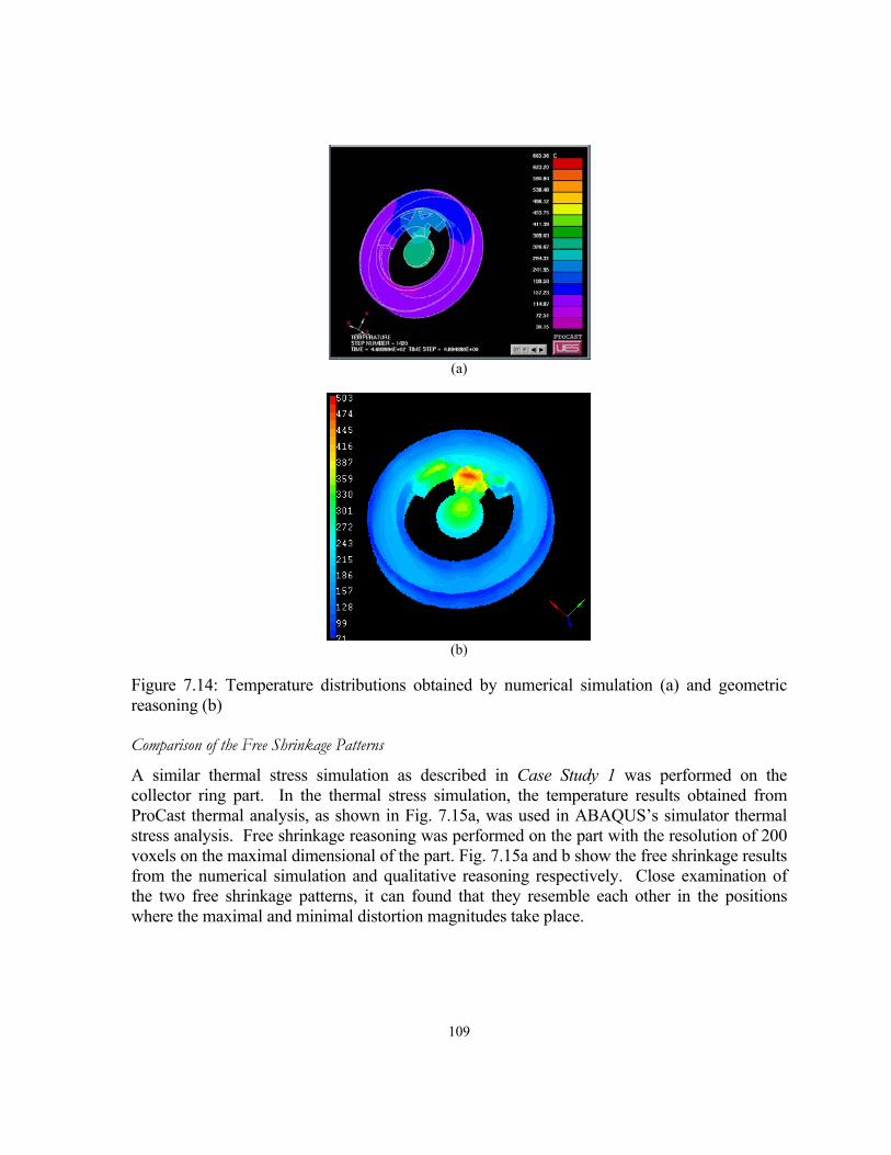
109

(a)

(b)

Figure 7.14: Temperature distributions obtained by numerical simulation (a) and geometric reasoning (b)

Comparison of the Free Shrinkage Patterns

A similar thermal stress simulation as described in Case Study 1 was performed on the collector ring part. In the thermal stress simulation, the temperature results obtained from ProCast thermal analysis, as shown in Fig. 7.15a, was used in ABAQUS’s simulator thermal stress analysis. Free shrinkage reasoning was performed on the part with the resolution of 200 voxels on the maximal dimensional of the part. Fig. 7.15a and b show the free shrinkage results from the numerical simulation and qualitative reasoning respectively. Close examination of the two free shrinkage patterns, it can found that they resemble each other in the positions where the maximal and minimal distortion magnitudes take place.

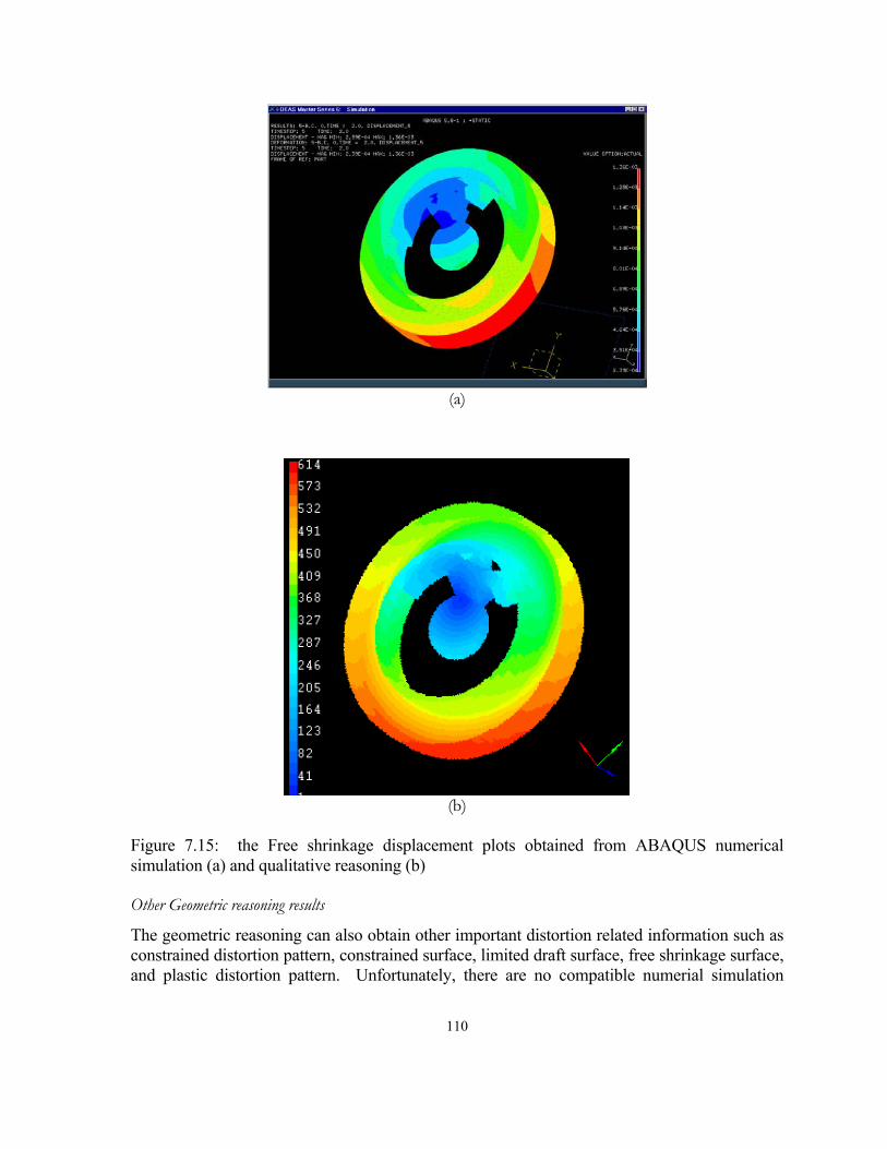
110

(a)

(b)

Figure 7.15: the Free shrinkage displacement plots obtained from ABAQUS numerical simulation (a) and qualitative reasoning (b)

Other Geometric reasoning results

The geometric reasoning can also obtain other important distortion related information such as constrained distortion pattern, constrained surface, limited draft surface, free shrinkage surface, and plastic distortion pattern. Unfortunately, there are no compatible numerial simulation

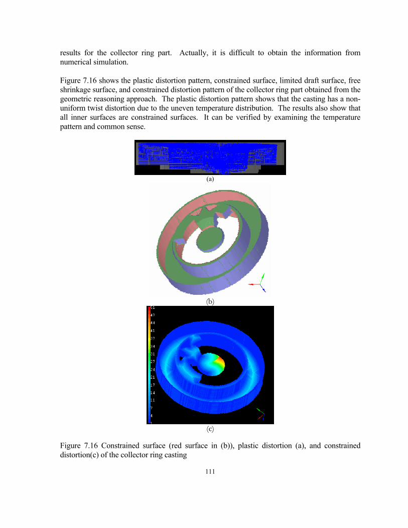
111

results for the collector ring part. Actually, it is difficult to obtain the information from numerical simulation.

Figure 7.16 shows the plastic distortion pattern, constrained surface, limited draft surface, free shrinkage surface, and constrained distortion pattern of the collector ring part obtained from the geometric reasoning approach. The plastic distortion pattern shows that the casting has a non-uniform twist distortion due to the uneven temperature distribution. The results also show that all inner surfaces are constrained surfaces. It can be verified by examining the temperature pattern and common sense.

(a)

(b)

(c)

Figure 7.16 Constrained surface (red surface in (b)), plastic distortion (a), and constrained distortion(c) of the collector ring casting

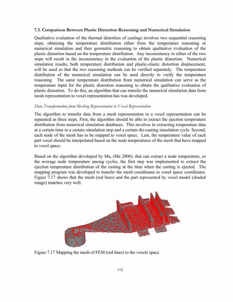
112

7.3. Comparison Between Plastic Distortion Reasoning and Numerical Simulation

Qualitative evaluation of the thermal distortion of castings involves two sequential reasoning steps, obtaining the temperature distribution either from the temperature reasoning or numerical simulation and then geometric reasoning to obtain qualitative evaluation of the plastic distortion based on the temperature distribution. Any inconsistency in either of the two steps will result in the inconsistency in the evaluation of the plastic distortion. Numerical simulation results, both temperature distribution and plastic-elastic distortion displacement, will be used so that the two reasoning methods can be verified separately. The temperature distribution of the numerical simulation can be used directly to verify the temperature reasoning. The same temperature distribution from numerical simulation can serve as the temperature input for the plastic distortion reasoning to obtain the qualitative evaluation of plastic distortion. To do this, an algorithm that can transfer the numerical simulation data from mesh representation to voxel representation has was developed.

Data Transformation from Meshing Representation to Voxel Representation

The algorithm to transfer data from a mesh representation to a voxel representation can be separated as three steps. First, the algorithm should be able to extract the ejection temperature distribution from numerical simulation databases. This involves in extracting temperature data at a certain time in a certain simulation step and a certain die-casting simulation cycle. Second, each node of the mesh has to be mapped to voxel space. Last, the temperature value of each part voxel should be interpolated based on the node temperatures of the mesh that have mapped to voxel space.

Based on the algorithm developed by Ma, (Ma 2000), that can extract a node temperature, or the average node temperature among cycles, the first step was implemented to extract the ejection temperature distribution of the casting at the time when the casting is ejected. The mapping program was developed to transfer the mesh coordinates to voxel space coordinates. Figure 7.17 shows that the mesh (red lines) and the part represented by voxel model (shaded image) matches very well.

Figure 7.17 Mapping the mesh of FEM (red lines) to the voxels space

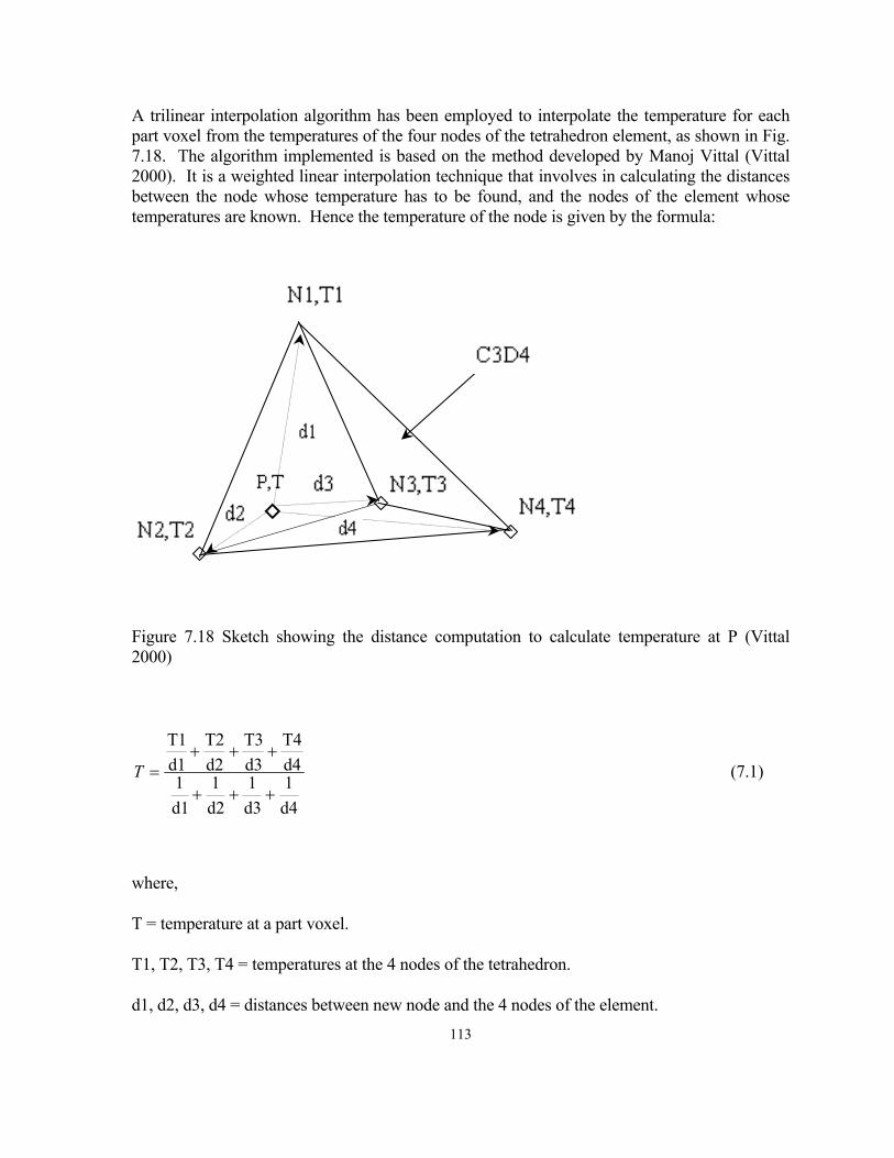
113

A trilinear interpolation algorithm has been employed to interpolate the temperature for each part voxel from the temperatures of the four nodes of the tetrahedron element, as shown in Fig. 7.18. The algorithm implemented is based on the method developed by Manoj Vittal (Vittal 2000). It is a weighted linear interpolation technique that involves in calculating the distances between the node whose temperature has to be found, and the nodes of the element whose temperatures are known. Hence the temperature of the node is given by the formula:

Figure 7.18 Sketch showing the distance computation to calculate temperature at P (Vittal 2000)

d41

d31

d21

d11

d4T4

d3T3

d2T2

d1T1

+++

+++=T (7.1)

where,

T = temperature at a part voxel.

T1, T2, T3, T4 = temperatures at the 4 nodes of the tetrahedron.

d1, d2, d3, d4 = distances between new node and the 4 nodes of the element.

114

Figure 7.19: The ejection temperature distribution of ABQUS numerical simulation represented in voxel space

Fig. 7.19 shows the temperature distribution in voxel space that was transferred from the temperature distribution represented by the FEM simulation based on the tetrahedron mesh. The temperature gradient on the skeleton of the casting will be used to calculate the plastic distortion. As a differential operator, the gradient operator will amplify the interpolation error and digitization error that comes from voxel representation of the temperature in voxel space. In order to reduce this errors, a 5×5×5 Gaussian filter has been applied on each voxel so that of temperature distribution can be smoothed when the temperature gradient is calculated. This temperature gradient distribution will be used to qualitatively evaluate plastic distortion as discussed in previous chapter.

Qualitative Evaluation of Thermal Plastic Distortion Based on the Temperature Distribution Obtained from

Numerical Simulation

The temperature distribution shown in Fig 7.19 was used to the qualitatively evaluate the thermal plastic distortion. Ten die-casting cycles have been simulated by Ragab (Ragab 2000), from the die casting group at OSU. The temperature distribution was extracted from the ABQUS simulation database using the last simulated die-casting cycle (cycle 10) at the point that the casting is ejected from the die. The elastic-plastic distortion obtained from the numerical is shown in Fig. 7.20a while the pure plastic distortion obtained from qualitative reasoning is shown in Figure 7.20b.

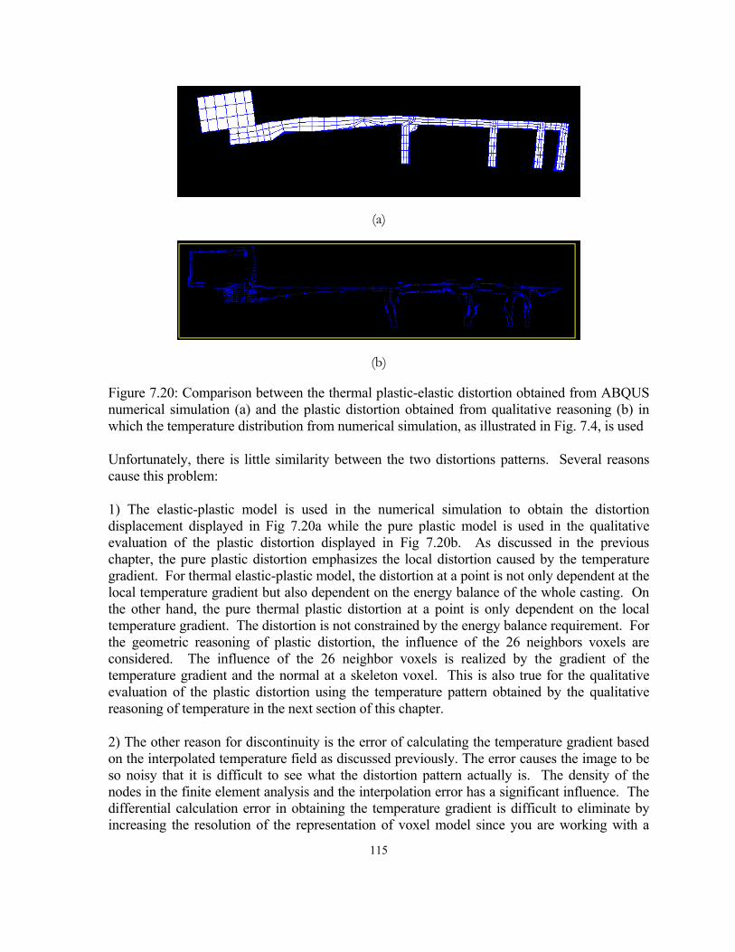
115

(a)

(b) Figure 7.20: Comparison between the thermal plastic-elastic distortion obtained from ABQUS numerical simulation (a) and the plastic distortion obtained from qualitative reasoning (b) in which the temperature distribution from numerical simulation, as illustrated in Fig. 7.4, is used

Unfortunately, there is little similarity between the two distortions patterns. Several reasons cause this problem:

1) The elastic-plastic model is used in the numerical simulation to obtain the distortion displacement displayed in Fig 7.20a while the pure plastic model is used in the qualitative evaluation of the plastic distortion displayed in Fig 7.20b. As discussed in the previous chapter, the pure plastic distortion emphasizes the local distortion caused by the temperature gradient. For thermal elastic-plastic model, the distortion at a point is not only dependent at the local temperature gradient but also dependent on the energy balance of the whole casting. On the other hand, the pure thermal plastic distortion at a point is only dependent on the local temperature gradient. The distortion is not constrained by the energy balance requirement. For the geometric reasoning of plastic distortion, the influence of the 26 neighbors voxels are considered. The influence of the 26 neighbor voxels is realized by the gradient of the temperature gradient and the normal at a skeleton voxel. This is also true for the qualitative evaluation of the plastic distortion using the temperature pattern obtained by the qualitative reasoning of temperature in the next section of this chapter.

2) The other reason for discontinuity is the error of calculating the temperature gradient based on the interpolated temperature field as discussed previously. The error causes the image to be so noisy that it is difficult to see what the distortion pattern actually is. The density of the nodes in the finite element analysis and the interpolation error has a significant influence. The differential calculation error in obtaining the temperature gradient is difficult to eliminate by increasing the resolution of the representation of voxel model since you are working with a

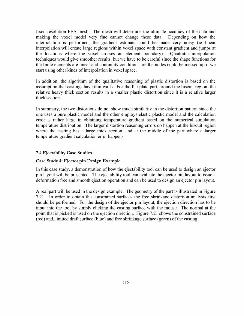
116

fixed resolution FEA mesh. The mesh will determine the ultimate accuracy of the data and making the voxel model very fine cannot change these data. Depending on how the interpolation is performed, the gradient estimate could be made very noisy (ie linear interpolation will create large regions within voxel space with constant gradient and jumps at the locations where the voxel crosses an element boundary). Quadratic interpolation techniques would give smoother results, but we have to be careful since the shape functions for the finite elements are linear and continuity conditions are the nodes could be messed up if we start using other kinds of interpolation in voxel space.

In addition, the algorithm of the qualitative reasoning of plastic distortion is based on the assumption that castings have thin walls. For the flat plate part, around the biscuit region, the relative heavy thick section results in a smaller plastic distortion since it is a relative larger thick section.

In summary, the two distortions do not show much similarity in the distortion pattern since the one uses a pure plastic model and the other employs elastic plastic model and the calculation error is rather large in obtaining temperature gradient based on the numerical simulation temperature distribution. The larger distortion reasoning errors do happen at the biscuit region where the casting has a large thick section, and at the middle of the part where a larger temperature gradient calculation error happens.

7.4 Ejectability Case Studies

Case Study 4: Ejector pin Design Example

In this case study, a demonstration of how the ejectability tool can be used to design an ejector pin layout will be presented. The ejectability tool can evaluate the ejector pin layout to issue a deformation free and smooth ejection operation and can be used to design an ejector pin layout.

A real part will be used in the design example. The geometry of the part is illustrated in Figure 7.21. In order to obtain the constrained surfaces the free shrinkage distortion analysis first should be performed. For the design of the ejector pin layout, the ejection direction has to be input into the tool by simply clicking the casting surface with the mouse. The normal at the point that is picked is used on the ejection direction. Figure 7.21 shows the constrained surface (red) and, limited draft surface (blue) and free shrinkage surface (green) of the casting.

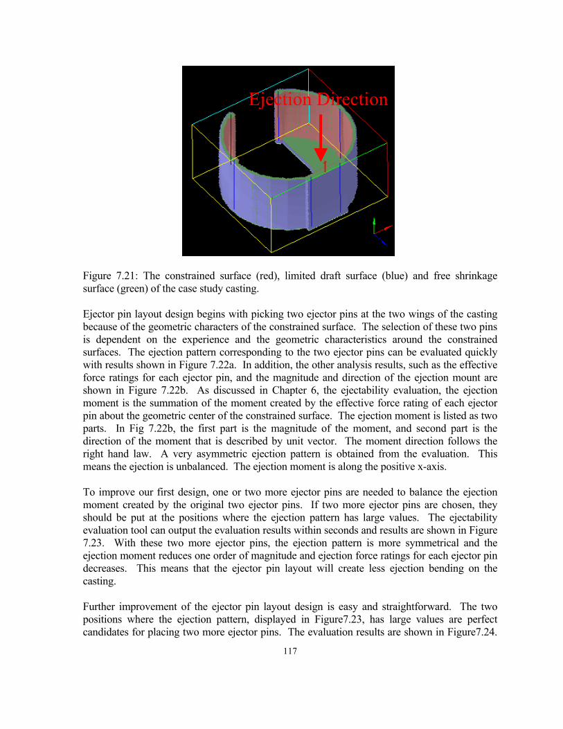
117

Ejection Direction

Figure 7.21: The constrained surface (red), limited draft surface (blue) and free shrinkage surface (green) of the case study casting.

Ejector pin layout design begins with picking two ejector pins at the two wings of the casting because of the geometric characters of the constrained surface. The selection of these two pins is dependent on the experience and the geometric characteristics around the constrained surfaces. The ejection pattern corresponding to the two ejector pins can be evaluated quickly with results shown in Figure 7.22a. In addition, the other analysis results, such as the effective force ratings for each ejector pin, and the magnitude and direction of the ejection mount are shown in Figure 7.22b. As discussed in Chapter 6, the ejectability evaluation, the ejection moment is the summation of the moment created by the effective force rating of each ejector pin about the geometric center of the constrained surface. The ejection moment is listed as two parts. In Fig 7.22b, the first part is the magnitude of the moment, and second part is the direction of the moment that is described by unit vector. The moment direction follows the right hand law. A very asymmetric ejection pattern is obtained from the evaluation. This means the ejection is unbalanced. The ejection moment is along the positive x-axis.

To improve our first design, one or two more ejector pins are needed to balance the ejection moment created by the original two ejector pins. If two more ejector pins are chosen, they should be put at the positions where the ejection pattern has large values. The ejectability evaluation tool can output the evaluation results within seconds and results are shown in Figure 7.23. With these two more ejector pins, the ejection pattern is more symmetrical and the ejection moment reduces one order of magnitude and ejection force ratings for each ejector pin decreases. This means that the ejector pin layout will create less ejection bending on the casting.

Further improvement of the ejector pin layout design is easy and straightforward. The two positions where the ejection pattern, displayed in Figure7.23, has large values are perfect candidates for placing two more ejector pins. The evaluation results are shown in Figure7.24.

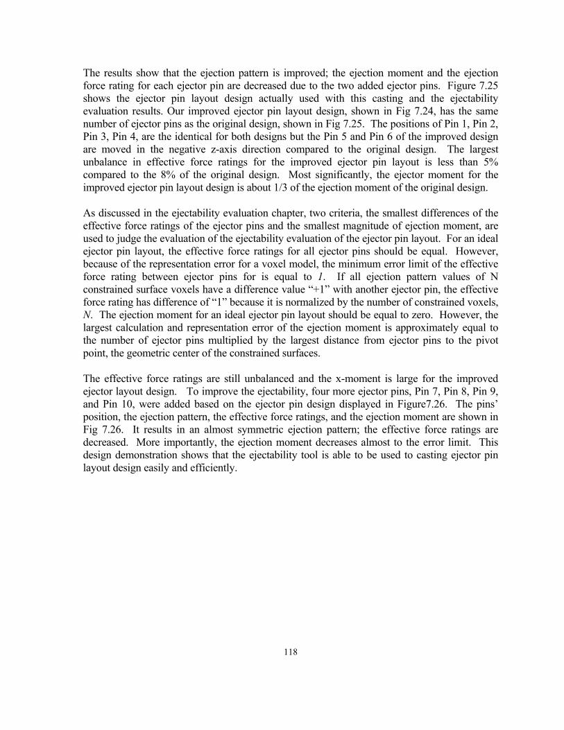
118

The results show that the ejection pattern is improved; the ejection moment and the ejection force rating for each ejector pin are decreased due to the two added ejector pins. Figure 7.25 shows the ejector pin layout design actually used with this casting and the ejectability evaluation results. Our improved ejector pin layout design, shown in Fig 7.24, has the same number of ejector pins as the original design, shown in Fig 7.25. The positions of Pin 1, Pin 2, Pin 3, Pin 4, are the identical for both designs but the Pin 5 and Pin 6 of the improved design are moved in the negative z-axis direction compared to the original design. The largest unbalance in effective force ratings for the improved ejector pin layout is less than 5% compared to the 8% of the original design. Most significantly, the ejector moment for the improved ejector pin layout design is about 1/3 of the ejection moment of the original design.

As discussed in the ejectability evaluation chapter, two criteria, the smallest differences of the effective force ratings of the ejector pins and the smallest magnitude of ejection moment, are used to judge the evaluation of the ejectability evaluation of the ejector pin layout. For an ideal ejector pin layout, the effective force ratings for all ejector pins should be equal. However, because of the representation error for a voxel model, the minimum error limit of the effective force rating between ejector pins for is equal to 1. If all ejection pattern values of N constrained surface voxels have a difference value “+1” with another ejector pin, the effective force rating has difference of “1” because it is normalized by the number of constrained voxels, N. The ejection moment for an ideal ejector pin layout should be equal to zero. However, the largest calculation and representation error of the ejection moment is approximately equal to the number of ejector pins multiplied by the largest distance from ejector pins to the pivot point, the geometric center of the constrained surfaces.

The effective force ratings are still unbalanced and the x-moment is large for the improved ejector layout design. To improve the ejectability, four more ejector pins, Pin 7, Pin 8, Pin 9, and Pin 10, were added based on the ejector pin design displayed in Figure7.26. The pins’ position, the ejection pattern, the effective force ratings, and the ejection moment are shown in Fig 7.26. It results in an almost symmetric ejection pattern; the effective force ratings are decreased. More importantly, the ejection moment decreases almost to the error limit. This design demonstration shows that the ejectability tool is able to be used to casting ejector pin layout design easily and efficiently.

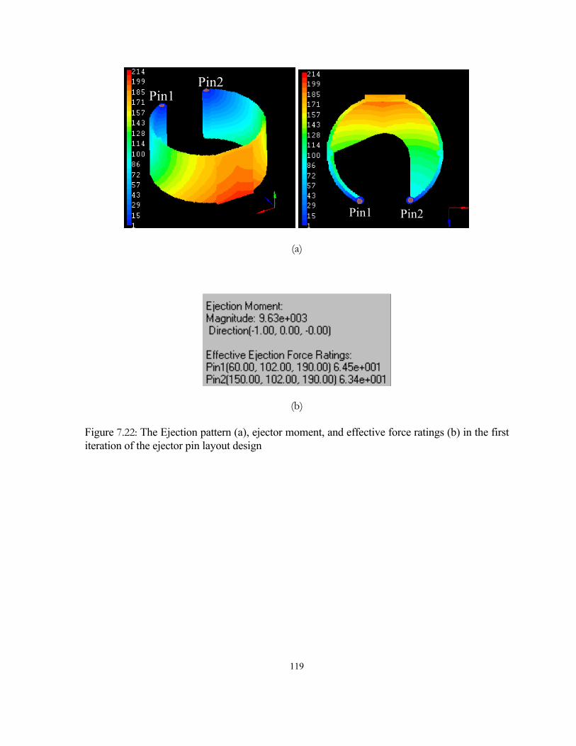
119

Pin1Pin2

Pin1Pin2

Pin1 Pin2Pin1 Pin2

(a)

(b)

Figure 7.22: The Ejection pattern (a), ejector moment, and effective force ratings (b) in the first iteration of the ejector pin layout design

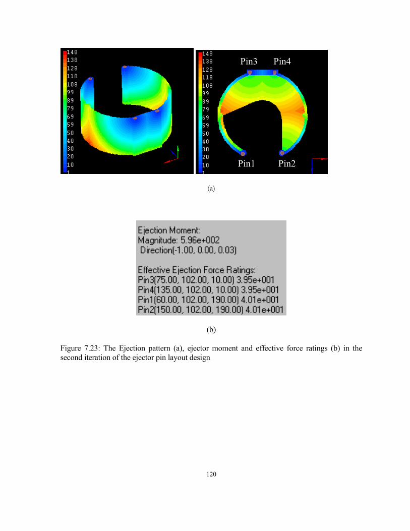
120

Pin1 Pin2

Pin3 Pin4

(a)

(b)

Figure 7.23: The Ejection pattern (a), ejector moment and effective force ratings (b) in the second iteration of the ejector pin layout design

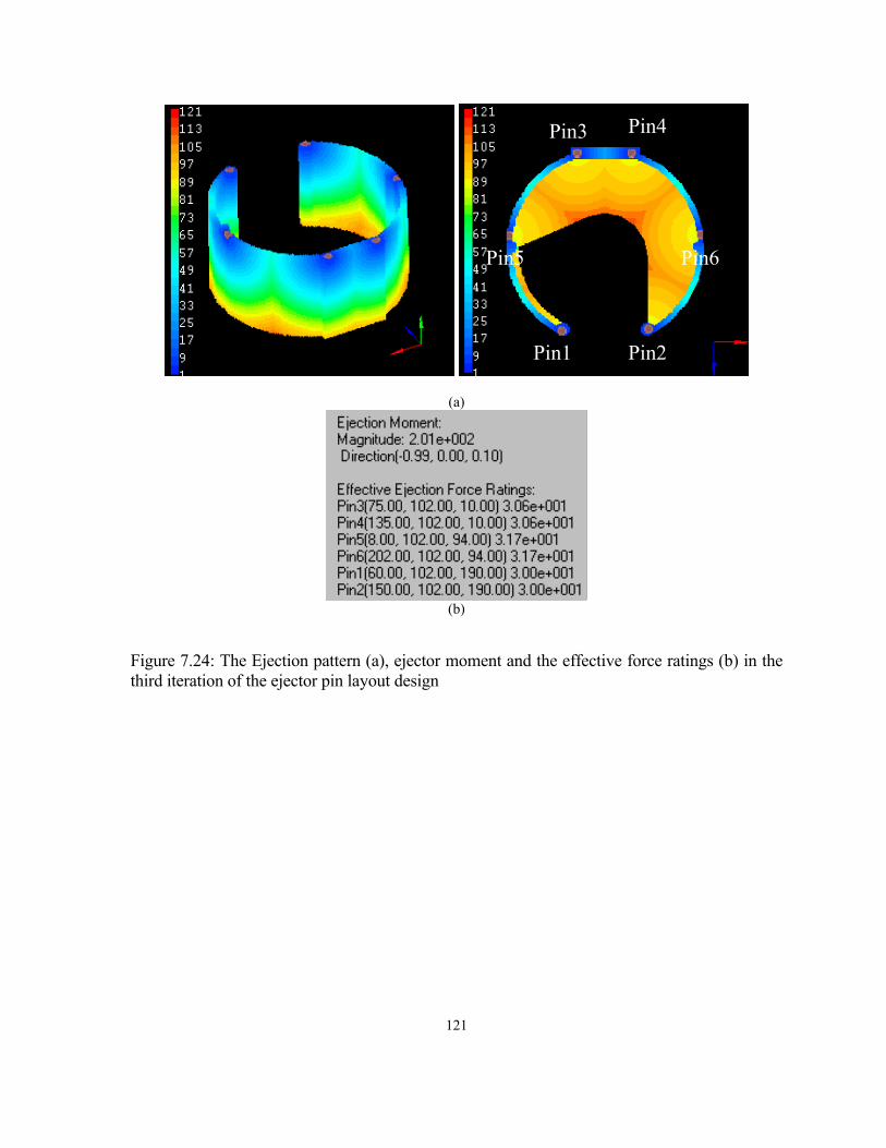
121

Pin5 Pin6

Pin1 Pin2

Pin3 Pin4

(a)

(b)

Figure 7.24: The Ejection pattern (a), ejector moment and the effective force ratings (b) in the third iteration of the ejector pin layout design

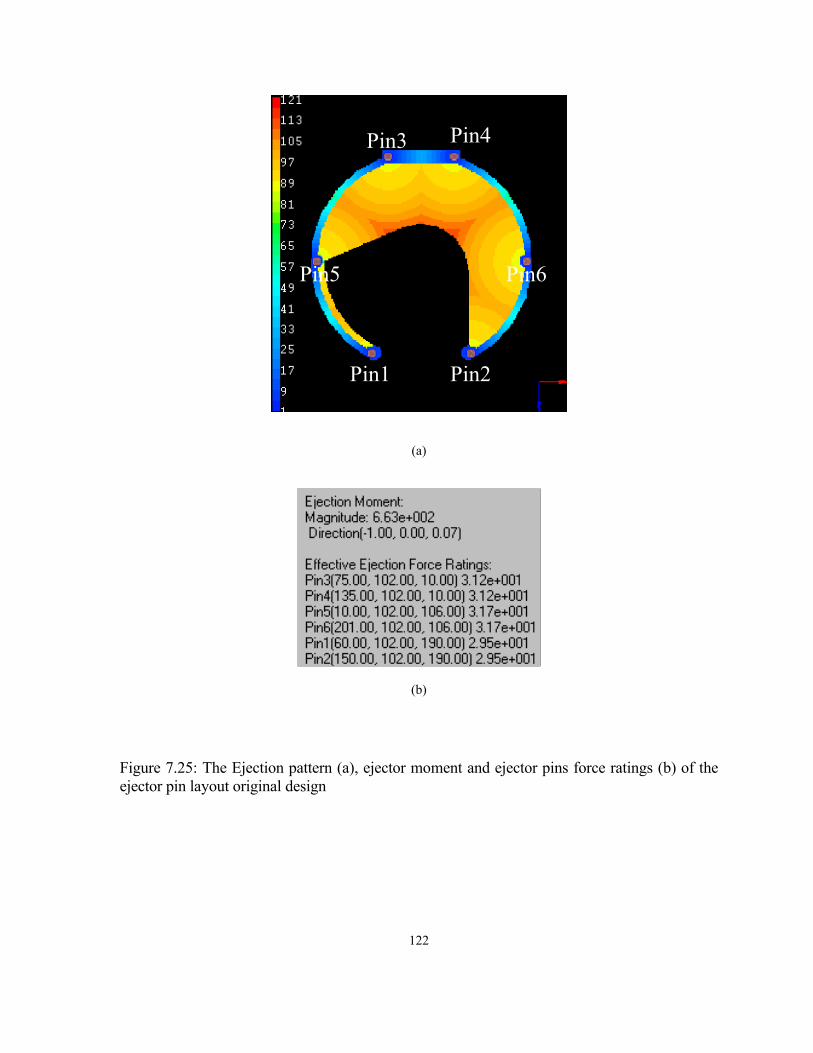
122

Pin5 Pin6

Pin1 Pin2

Pin3 Pin4

(a)

(b)

Figure 7.25: The Ejection pattern (a), ejector moment and ejector pins force ratings (b) of the ejector pin layout original design

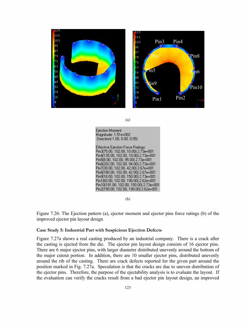
123

Pin5 Pin6

Pin8

Pin10Pin9

Pin1 Pin2

Pin7

Pin3 Pin4

(a)

(b) Figure 7.26: The Ejection pattern (a), ejector moment and ejector pins force ratings (b) of the improved ejector pin layout design

Case Study 5: Industrial Part with Suspicious Ejection Defects

Figure 7.27a shows a real casting produced by an industrial company. There is a crack after the casting is ejected from the die. The ejector pin layout design consists of 16 ejector pins. There are 6 major ejector pins, with larger diameter distributed unevenly around the bottom of the major cutout portion. In addition, there are 10 smaller ejector pins, distributed unevenly around the rib of the casting. There are crack defects reported for the given part around the position marked in Fig. 7.27a. Speculation is that the cracks are due to uneven distribution of the ejector pins. Therefore, the purpose of the ejectability analysis is to evaluate the layout. If the evaluation can verify the cracks result from a bad ejector pin layout design, an improved

124

ejector pin layout design should be evaluated. In order to evaluate the ejector pin layout, a simplified CAD model, which is shown in Fig 7.27, was constructed. The CAD model contains all the major features of the real part.

The free shrinkage pattern and constrained surfaces were first obtained by the geometric reasoning and are shown in Figure 7.27b and c. From the characteristics of constrained surface, it can be seen that the constrained surfaces are distributed around the rib of the casting and inside of the holes.

Figure 7.28a shows the results if only the 6 major ejector pins are used in the evaluation. These unevenly distributed ejector pins do create an ejection moment so that the part can bend during ejection. From the ejection pattern (Figure 7.28a), it can be seen that there is large ejection resistance near the place where the cracks occur.

However, a close examination of the evaluation results for the 10 small ejector pins, which is displayed in Figure 7.28b, shows a different result. The 10 small pins also create an uneven ejection pattern and potential bending in almost the opposite direction of that created by the 6 major ejector pins.

If all the 6 major ejector pins and 10 minor ejector pins are used in the ejectability evaluation, the analysis results are shown in Figure 7.28c. A pretty symmetric dejection pattern is observed. In the ejectability evaluation, an implicit assumption has been made that all pins provide the same ejection force. The largest difference of the effective force ratings between ejector pins is about 2. That is very close to the error limit 1, as discussed in previous ejectability evaluation case study, which is the ejectability evaluation error limit caused by the voxel model. The relative error about the effective force rating is about 10%. Furthermore, due to the evaluation error of the effective force rating, the magnitude of the ejection moment is also within the evaluation error of the ejection moment. The average moment arm about the geometric center of the constrained surfaces is about 70 (the actual diameter of the disk is 200, voxel size is 0.985). If the difference of the effective force rating at the opposite position about x-axis is equal to one, 70 of the ejection moment magnitude will results. Actually, it can be found that the effective force rating of the pins at positive direction of x-axis is larger than that on the negative direction (For example, Pin 12 and Pin 13, Pin 14 and Pin 1, Pin 3 and Pin 4, Pin7 and Pin8,…). This causes the evaluation error of the ejection moment and this is the reason that the ejection moment is at y-direction.

In summary, within the evaluation error limitation, the evaluation of the ejectability of the ejector pin layout design shows that the ejector pin layout does have potential to provide a balanced ejection. The original design is a good design and the cracks may not result from a poor ejector pin layout design.

125

Discontinuity

(a)

(b) (c)

Figure 7.27: The simplified CAD model for the Part (a), free shrinkage displacement pattern (blue image in (c)), constrained surfaces and limited draft surfaces, and free shrinkage surfaces (red surfaces, blue surfaces, and green surfaces in (b) respectively)

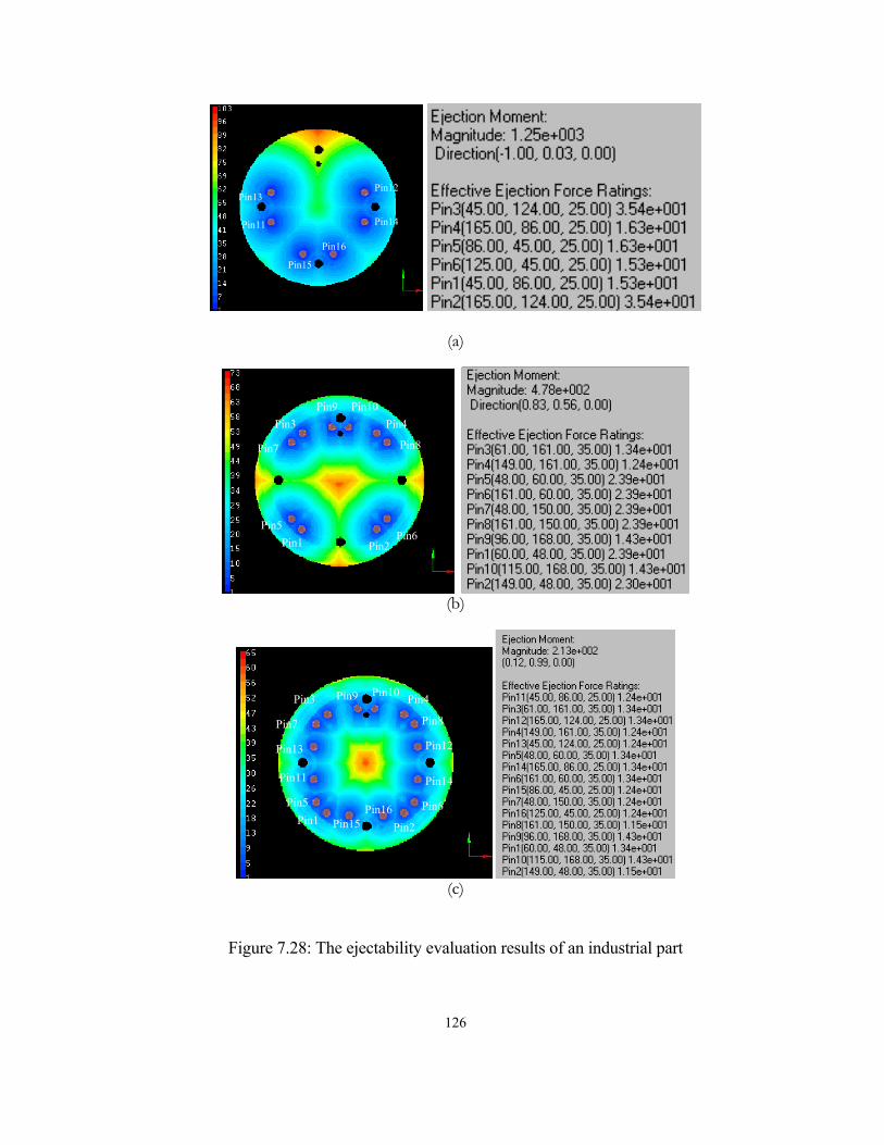
126

Pin12

Pin14

Pin15

Pin16

Pin11

Pin13

(a)

Pin1

Pin10Pin4

Pin8

Pin6Pin2

Pin7

Pin3Pin9

Pin5

(b)

Pin1

Pin10 Pin4

Pin8

Pin12

Pin14

Pin6

Pin2

Pin7

Pin3 Pin9

Pin15Pin16Pin5

Pin11

Pin13

(c)

Figure 7.28: The ejectability evaluation results of an industrial part

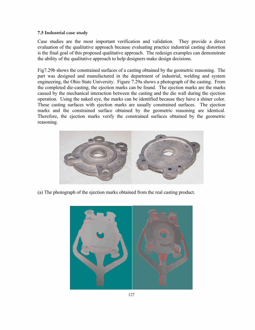
127

7.5 Industrial case study

Case studies are the most important verification and validation. They provide a direct evaluation of the qualitative approach because evaluating practice industrial casting distortion is the final goal of this proposed qualitative approach. The redesign examples can demonstrate the ability of the qualitative approach to help designers make design decisions.

Fig7.29b shows the constrained surfaces of a casting obtained by the geometric reasoning. The part was designed and manufactured in the department of industrial, welding and system engineering, the Ohio State University. Figure 7.29a shows a photograph of the casting. From the completed die-casting, the ejection marks can be found. The ejection marks are the marks caused by the mechanical interaction between the casting and the die wall during the ejection operation. Using the naked eye, the marks can be identified because they have a shiner color. These casting surfaces with ejection marks are usually constrained surfaces. The ejection marks and the constrained surface obtained by the geometric reasoning are identical. Therefore, the ejection marks verify the constrained surfaces obtained by the geometric reasoning.

(a) The photograph of the ejection marks obtained from the real casting product.

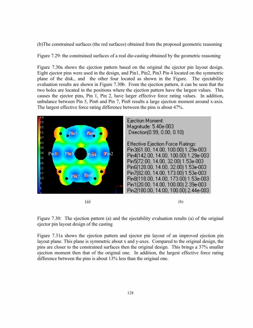
128

(b)The constrained surfaces (the red surfaces) obtained from the proposed geometric reasoning

Figure 7.29: the constrained surfaces of a real die-casting obtained by the geometric reasoning

Figure 7.30a shows the ejection pattern based on the original the ejector pin layout design. Eight ejector pins were used in the design, and Pin1, Pin2, Pin3 Pin 4 located on the symmetric plane of the disk., and the other four located as shown in the Figure. The ejectability evaluation results are shown in Figure 7.30b. From the ejection pattern, it can be seen that the two holes are located in the positions where the ejection pattern have the largest values. This causes the ejector pins, Pin 1, Pin 2, have larger effective force rating values. In addition, unbalance between Pin 5, Pin6 and Pin 7, Pin8 results a large ejection moment around x-axis. The largest effective force rating difference between the pins is about 47%.

Pin5 Pin6

Pin8

Pin1 Pin2

Pin7

Pin3 Pin4

(a) (b)

Figure 7.30: The ejection pattern (a) and the ejectability evaluation results (a) of the original ejector pin layout design of the casting

Figure 7.31a shows the ejection pattern and ejector pin layout of an improved ejection pin layout plane. This plane is symmetric about x and y-axes. Compared to the original design, the pins are closer to the constrained surfaces then the original design. This brings a 37% smaller ejection moment then that of the original one. In addition, the largest effective force rating difference between the pins is about 13% less than the original one.

129

Pin5 Pin6

Pin8

Pin1 Pin2

Pin7

Pin3 Pin4

Pin5 Pin6

Pin8

Pin1 Pin2

Pin7

Pin3 Pin4

(b) (b)

Figure 7.31: The ejection pattern (a) and the ejectability evaluation results (a) of the first improved ejector pin layout design of the casting

For the real casting, rearranging the ejector pin positions can improve of the ejectability of the casting. Because of the geometric or functionality constrictions, not all positions are available to put an ejector pin. This case study shows that the evaluation tool can be used to improve the ejector pin design so that the ejectability of the casting can be improved.

130

8. CONCLUSIONS

8.1 Summary of Research Contribution

The importance of design-for-manufacturability is well understood today. However, “over the wall” designs are still common. The majority of designers consider only the functional requirements and pass manufacturing problems downstream. They are reluctant to predict the optimum design and rely primarily on feedback from experts for manufacturing-related improvements. The primary reason for this is the lack of proper design evaluation tools that designers can understand and are comfortable using. In this research, a new approach for qualitative evaluation of the thermal distortion of castings was developed to support design-for-manufacturability evaluation in die-casting manufacturing processes. In contrast to evaluation using numerical simulations, this approach provides results based only on the overall part geometry. It provides a fast yet thorough evaluation of the part design in terms of manufacturing relevant geometric characteristics. Volumetric part representations and their associated processing techniques, such as distance transformation, have proved to be very efficient to extract thermal distortion related geometric characteristics. The resulting tool is very efficient in terms of computation time, and can evaluate the design regardless of shape complexity. In addition, it is very simple to use and the results are self-evident. Consequently, it can be used long before any other available tools, resulting in significant reductions in cost and effort. The contributions of this research are briefly listed as follows:

1. This research proposes a new and systematic methodology to deal with distortion evaluation problems in die-casting manufacturing processes. The manufacturability concerns of the die casting process are first identified. These concerns are then characterized in terms of corresponding geometrical properties. Specifically, the geometric characteristics that are often responsible for die casting thermal distortion related problems are constrained surfaces of the part and free shrinkage surfaces of the part. These geometric characteristics are then extracted based on a suitable part model, in this case a voxel model. The results are then presented through a specifically tailored visualization system.

2. The voxel-based model was identified as the part representation scheme to support the extraction of geometric characteristics for diecastability evaluation. Voxel-based models have the unique advantage of being able to model not only the surface but also the interior of an object explicitly. The latter simplifies the extraction of volume-related geometric characteristics. In addition, the uniformity makes it especially beneficial for applications that

131

involve complex geometries. These properties have facilitated the development of design tools hitherto not possible.

3. Qualitative analyses about the casting distortion related phenomenon such as free shrinkage, constrained distortion, thermal plastic distortion, heat conduction, have been performed. Based on the analyses, the qualitative distortion patterns associated with each of the phenomenon have been defined based on the volume potential theory. Several distortion centers that are linked to the geometric characteristics of the parts were also defined so that the distortion patterns can be extracted by geometric reasoning without the material and process data.

4. A new 3-D Euclidean distance transform algorithm to facilitate fast, less memory expensive determination of Euclidean distance was presented. The new algorithm can be used not only in performing thickness section analysis but also in evaluating the volume potential required for temperature and distortion.

5. A new algorithm that can quickly and easily identify the component at the skeleton normal direction of a vector field has been developed. Therefore, this algorithm can facilitate the evaluation of the skeleton distortion and shaded display of the skeleton.

6. An evaluation tool has been developed based on the geometric reasoning approach to evaluate the ejectability of a casting ejector pin layout design. It can be used in both the evaluation of ejector pin layouts and redesign of an exiting design. Several ejectability functions have been defined and implemented to facilitate the ejectability evaluation. The ejectability evaluation depends only on casting’s geometric information and the ejector pin layout design as well as the parting line position and ejection direction. Therefore, the tool can be used to help die casters make decision about the locations of ejection pins and parting line to issue a deformation free and smooth ejection operation.

8.2 Suggestion for Future Work

In this research, the geometric reasoning to qualitatively evaluate the thermal distortion of castings has been developed. In contrast to conventional CAE tools, geometric reasoning is much easier to use and more efficient so that it is suitable to support design for manufacturing. All results of the geometric reasoning, constrained surfaces or temperature pattern, free shrinkage pattern, constrained shrinkage pattern and plastic distortion pattern are the geometric attributes of a casting. The attributes are relevant to the thermal distortion of castings. When casting designers define the geometry of their casting designs, the geometric characteristics are defined. Therefore, this geometric reasoning is very natural to support design for manufacturing. By using digital data processing techniques, i.e. distances transform and

132

contextual distortion, the geometric characteristics are extracted. An evaluation tool for ejector pin layout is developed. This tool can help die designers to evaluate the ejector pin layout and help to make design decision. Since the thin wall geometry of the castings has been assumed in the geometric reasoning, the geometric reasoning may not produce reasonable results for the castings with larger wall thickness change.

The methodology developed in this research can be applied to many similar problems in design and manufacturing. Another future work of this research should involve extending this approach to cover the cooling sequence of castings. In the geometric reasoning, the temperature pattern is the description of the average temperature. Temperature history during the casting cooling is critical to study the thermal distortion of castings. Another potential extension of this research is retrieving more thermal distortion related information from the geometric reasoning results. For example, from the constrained shrinkage pattern, one may obtain the residual stress information caused by the constrained of the die wall.

133

REFERENCES

Anselman, George W., A. M. P, Joseph Cunningham, Victor Rowell, Richard A. Green, LeRoy E. Talor, James C. Lee, Charles W. Ward, Edwin H. Phelps Ezar L. Kotzin (1974), "Analysis of Casting Defects", Des Plaines, ILL, American Foundrymen's Society.

Bajscsy, R. (1989), “Multiresolution Elastic Matching”, CVGIP, vol. 46:1-21

Bellet, Michel, M. M., Francois Bay (1993), "Finite Element Modeling of the Cooling Phase in Casting Processes", Modeling of Casting, Welding and Advanced Solidification Processes-VI. V. V. T. S. Piwonka, L. Katgerman. Warrebdeake, Pennsylvania, USA, A Publication of the Minerals, Metals & Materials Society: 519-534.

Blum, H., (1967), “A Transformation for Extracting New Descriptors of Shapes”, Wathen-Dunn, W. (Ed), Models for the perception of Speech and Visual Form, M.I.T. Press.

Boley, B.A. and Weiner, J.H.(1960), “Theory of Thermal Stress”, John, Wiley & Sons, inc., New York, London.

Borgefors, G. (1984), “Distance Transformations in Arbitrary Dimensions”, Comput. Vision, Graphics, Image Processing, vol. 27, 321-345

Calladine, C.R. (1969), “Engineering Plasticity”, Perganon Press, Oxford, London, New York.

Campbell, J. (1993), "Solidification Modeling: Current Limitations and Future Potential", Modeling of Casting, Welding and Advanced Solidification Processes-VI. V. V. T. S. Piwonka, L. Katgerman. Warrebdeake, Pennsylvania, USA, A Publication of the Minerals, Metals & Materials Society: 519-534.

Celentana, Diego S. O., Eugunio Onate (1996), “A Coupled Thermomechanical Model for the Solidification of Cast Metals”, International Journal of Solids Structures 33(5): 747-763.

Chu, C. N., J. M. L., R. L. Kashyap, (1993), “Skeleton-Based Design Analysis of Near Net-shaped Process”, Anals of the CIRP 42: 193-196.

Cross, M. (1993), "Development of Novel Computational Techniques for the Next Generation of Software Tools for Casting Simulation", Modeling of Casting, Welding and Advanced Solidification Processes-VI. V. V. T. S. Piwonka, L. Katgerman. Warrebdeake, Pennsylvania, USA, A Publication of the Minerals, Metals & Materials Society: 519-534.

Cui, Dehua, Manoj Vittal, R. Allen Miller (1999), "Thermal Distortion Evaluation by 3D Geometric Reasoning", Transactions, NADCA Congress Sections, Cleveland, Ohio 1999.

134

Cui, D., Miller ,R.A, “Casting Ejectability Evaluation by 3D geometric Reasoning”, Transactions, NADCA Congress Sections, Rosemont, Illinois, 2000

Fryer, Y. D., C. B., M Cross, P Chow (1993), "Predicting Macro Porosity in Shape Castings Using an Integrated Control Volume Unstructured Mesh (CV-UM) FrameWork", Modeling of Casting, Welding and Advanced Solidification Processes-VI. V. V. T. S. Piwonka, L. Katgerman. Warrebdeake, Pennsylvania, USA, A Publication of the Minerals, Metals & Materials Society: 519-534.

Gupta, Satyandra K., D. D., William C. Regli, Dana S. Nau (1995), "Current Trends and Future Challenges in Automated Manufacturability Analysis", Computer in Engineering, Database Symposium, New York, The American Society of Mechanical Engineers.

Herman, E. A. (1985), "Die Casting Die: Designing", SDCE.

Housner, George W. and Thad Verrland, J. (1966), "The Analysis of Stress and Deformation", New York, London, The Macmillan Company.

Incropera, F. P., (1990), “Introduction to Heat Transfer”, New York, Chichester, Brisbane, Toronto, Singapore, John Wiley & Sons.

Johns, D. J. (1965), "Thermal Stress Analysis", Oxford, London, Edinburgh, New York, Frankfurt, Pergamon

Kim,K.Y.,Sakuta,T.,Suzuki,Y.,Umeda,T.,Kobayashi,T.,Tateishi,M.(1991)“deformation Analysis of AL-7%Si,0.3 Mg ”Modeling ofCasting,Welding and Advanced Solidification Processes V,The Minerals,Metals &Materials Society 259-264.

Kong, T. T., A. R. (1989), “Digital Topology: Introduction and Survey”, Computer vision, Graphics and Image Processing 48: 357-393.

Kozinska, D. (1998), “Multidimensional Alignment Using the Euclidean Distance Transform”, Graphical Models and Image Processing, vol. 59, No. 6:373-388

Kuipers, B. (1994), "Qualitative Reasoning, Modeling and Simulation with Incomplete Knowledge", Cambridge, Massachusetts, London, England, The MIT Press.

Lee, Ta-Chin, R. L. K., Chong-Nam Shu (1994), “Building Skeleton Models via 3-D Medial Surface/Axis Thinning Algorithms”, CVGIP Graphical Models and Image Processing 56(6): 562-478.

Lee, Ta-Chin (1994), “Building Skeleton Model via 3-D Medial Surface/Axis Thinning Algorithm”, Graphic Models and Image Processing 56(6):462-478

135

Lobregt, R (1980), “Three-Dimensional Skeletonization: Principle and Algorithm”, IEEE Transactions on Pattern Analysis and Machine Intelligence. PAMI-2 (1), 156-158

Lu, S.C. (1996), “Volume-based Geometric Reasoning and Visualization to Support Manufacturability Evaluation in Die-Casting”, The Ohio State University.

Lu, S. C., A. B. R., R. A. Miller, and G. L. Kinzel, R. Yagel (1995), "A Volume-Based Geometric Reasoning Approach for Diecastablity Evaluation", Proceedings of the Computers in Engineering Conference and the Engineering Database Symposium ASME 1995, Boston, Massachusetts, The American Society of Mechanical Engineers.

Ma, Yuming (2000), “ Thermal analysis of die casting die”, the Ohio State University PH.D. Dissertation

Mo, Asbjorn E. J. H. (1991), “On the Use of Constitutive Internal Variable Equations for Thermal Stress Predictions in Aluminum Casting”, Journal of Thermal Stresses 14: 571-587.

Morterson, M. E. (1995), "Geometric Modeling", New York, Chichester, Brisbane, Toronto, Singapore, John Wiley & Sons.

Ragnemalm, I. (1993), “The Euclidean Distance Transform in Arbitrary Dimensions”, Pattern Recognition Letters, vol. 14, 883-888

Rebello, A. B., S. C. Lu, R. A. Miller,(1995), “Integration of Design Manufacturability Analysis for Die Casting Design Systems”, pp. 123–130, Transactions 18th International Die Casting Congress and Exposition, North American Die Casting Association, Rosemont, Illinois, October

Rebello, Alexander B., S C. L., R. Allen Miller (1996), "Integration of Design Manufacturability Analysis for Die Casting Design System", Die Casting Innovation, Indianapolis, Indiana, and USA.

Rebello, A. B. (1997), "Visualization of the Filling of Die Casting Dies", The Ohio State University.

Shareef, Naeem R. Y. (1994), “Rapid Previewing via Volume-Based Solid Modeling”, Submitted to Solid Modeling (November).

Sully, L. J. D. (1978) "Die Casting", Oxford, London, New York , Perganon Press

Thomas, B. G. (1995), “Issue in Thermal-Mechanical Modeling of Casting Processes”, ISIJ international 35(N. 6): 737-743.

Thomas, B. G. (1993), "Stress Modeling of Casting Processes: An Overview", Modeling of Casting, Welding and Advanced Solidification Processes-VI. V. V. T. S. Piwonka, L.

136

Katgerman. Warrebdeake, Pennsylvania, USA, A Publication of the Minerals, Metals & Materials Society: 519-534.

Tikhonov, A.N., and Samarskii, A.A., (1963), "Equations of Mathematical Physics", New York, Dover Publication, Inc.

Upadhya, Cirish K. S. D., Anand J. Paul, (1994), “Geometric Methods for Simulation Solidification Heat Transfer in Casting Processes: Principles and Applications”, ASME HTD-Vo.l275 (Current Developments in Numerical Simulation and Heat Transfer): 43-54..

Yagel, R., S. C. L., A. B. Rebello, R. A. Miller (1995), “Volume-Based Reasoning and Visualization of Diecastability”, IEEE: 359-362.

Ye, Qin-Zhong (1988), “The Signed Euclidean Distance Trasform and Its Applications”, Proc. 9-th International Conference on Pattern Recognition, 405-400

qualitative reasoning for additional die casting …/67531/metadc736140/m2/1/high...qualitative...

Documents