408

The 4th International ConferenceAdvanced Composite Materials Engineering

COMAT 201218- 20 October 2012, Brasov, Romania

QUALITATIVE STUDY OF THE STRUCTURAL INFLUENCE OF THEFORCES ON THE STABILITY OF DYNAMICAL SYSTEMS

M. Lupu1 , O. Florea1 , C. Lupu2

1 Transilvania University of Brasov, Brasov, Romania,m.lupu@unitbv.ro, olivia.florea@unitbv.ro2Politehnica University of Bucharest, Bucharest,Romania, cip@indinf.pub.ro

Abstract: In this paper consider the autonomous dynamical system linear or linearized with 2 degree of freedom. In thesystem of equation of 4th degree, appear the structure generalized forces: - the conservative forces, - the non-conservative forces, the dissipative forces, the gyroscopically forces. In the linear system, these forces from thedifferent structural combinations can produce the stability or the instability of the null solution. In this way are known thetheorems of Thomson - Tait - Cetaev (T-T-C) for the configurations . We will introduce the non conservative forces

, studying the stability with the Routh - Hurwitz criterion or construct the Liapunov function, obtaining some theorems withpractical applications.Keywords: qualitative theory, stability, system structures, decomposition.

1. INTRODUCTION

In this section study the structural influence of the terms blocks on the stability of the null solution for the bi-dimensional system or equations with fourth degree, which is a linear or linearized system in first approximationfor the nonlinear system [2], [4].

(1)

In this system the matrix blocks are representing respectively the conservative (elastic) forces,the resistance (amortization) forces, the gyroscopically forces and the non-conservative forces. The characteristicpolynomial for the Routh - Hurwitz criterion will be [1], [7]:

(2)

The system (1) can be bring to the canonic form and making abstraction by the constant negative factor thestated forces will be respectively side by the system :

,,,

.Regarding this system there are classical contributions of the Liapunov and the theorems of Thomson - Tait -Cetaev [4], Merkin [2] and Crandall [4]. Here we’ll distinguish these results and we’ll make other structuralcontribution by examples.In the matricial calculus are known the decomposition theorems of the squared matrix. Any squared matrix canbe decompose in a sum of one symmetric matrix and the other one asymmetric . where

, .

From the decomposition theorem and using the fact that the positional forces are conservative with

409

, and and we have thecondition of symmetry and asymmetry .We have the relations:

(3)The system (3) has the fourth degree, and the characteristic polynomial is:

(4)

(5)

The system with constant coefficients (1) becomes:

(6)

The mechanical justification of this configuration is obtain starting from the Lagrange equations:

(7)

where is the kinetic energy, are the generalized force and are generalized forces with superiororder terms. So, the decomposition mentioned become symbolic for the positional forces and the inertial forces.

(8)where , with the potential energy, isthe function of dissipation with mechanical work negative, the conservative forces, ,

with mechanical work null. The system is completely dissipative if is the squared formpositive defined, and .

Theorem 1. If then the expression of the block is:Theorem 2. If then the expression of the block is:On the base of this structure of forces we’ll analyze the stability, making some

combinations of these forces, and we’ll obtain a series of theorems. For the system , Thomson - Tait -Cetaev (T-T-C)has defined the theorems.The examples are for the gyroscopes, bearings on the fluid support, double pendulum, electron in the magneticfield, the car equation and other examples from different domains making analogies for the system of the fourthdegree.Will note in the next theorem with the system (ex. - the system compose of and ), with thestable case, with the asymptotic case, and with the unstable case, using directly the characteristicpolynomial (5) (H-R) or the Liapunov function for (6).

2. THE STUDY OF THE STABILITY OF THE DYNAMICAL SYSTEMS

For start we will consider the stability of the equilibrium position in the point of minimum of the potentialenergy (the theorem Lagrange-Dirichlet) with slight oscillations around this position. We note with thecase of the cyclical coordinates in the phases plane when is obtain an uniform movement in report with these.Using the equations of Routh - Hurwitz - the case Lagrange - Poisson, for the solid with a fixed point (thegyroscop) is studied the stability of the uniform movements.Theorem 3. If the dynamical system is dynamical stable around of . (Ex.:

the mathematical pendulum in the graviphic field)

Observation 1. If is stable then is stable.Observation 2. If is non stable then is non stable.Theorem 4. (T-T-C) In the conservative system, if potential energy has an isolated minimum, then the system issimple stable around the minimal point: if If is stable around the zeropoint.

410

Theorem 5. (T-T-C) If we have an isolated potential simple stable then by attach to the system the dissipativeforces the the simple stability is keep; if the dissipation is total then the system become asymptotic stable: ifis stable , is complete dissipative, and in this case the system isasymptotic stable.Theorem 6. (T-T-C) In an instable potential regime in the vicinity of a maximum point for the potential energy,when this energy is negative, if are applied the dissipative force the instability is keep: if is unstable then

is unstable:The theorems (3-6) are verified directly with the Routh - Hurwitz criterion for the system (13).Theorem 7. If is stable then we have an uniform movement stable of (stability about ). Ex.: the caseLagrange - Poisson, the Routh method when we have the rotation angle and the precession angle cyclicallyimplies the uniform movement.Theorem 8. If the stability is conserve compared with the coordinates and with the speeds.Corollary 1. If in the time of the stable movement the stability will be lost just compared with thecoordinates, but not compared with the speeds.Corollary 2. If the system is nonlinear under the acting on and stable with then is not implicatethe stability for the non linear system.Theorem 9. (T-T-C) If the system is conserve for the coordinates and speeds and for the nonlinear system.Theorem 10. If we are acting with non-potential forces then the system is unstable . (seethe Application 1)Theorem 11. If we have the system then the system is unstable.Theorem 12.1. For the system we make the next hypothesis: if the system is stable then is perturbed(can be stable and unstable).2. If the system is stable or unstable then the system is perturbed (can be stable andunstable).Theorem 13. The dissipative forces can influenced on the stability so: if is unstablethen can be stabilized; if is stable then can be destabilized.Theorem 14. If in the system the two equations of second degree has the frequencies equal and byintroducing for the system we have: if the system are linear then the stability isperturbed indifferent of the nonlinear terms.Theorem 15. If is unstable then is stable.It is observe that the theorem T-T-C do not conserve always if appear the non-potential forces from Merkin[2].Application1. (Theorem 10)A system which has just the non-potential forces is always unstable. Such a system is represented by equations:

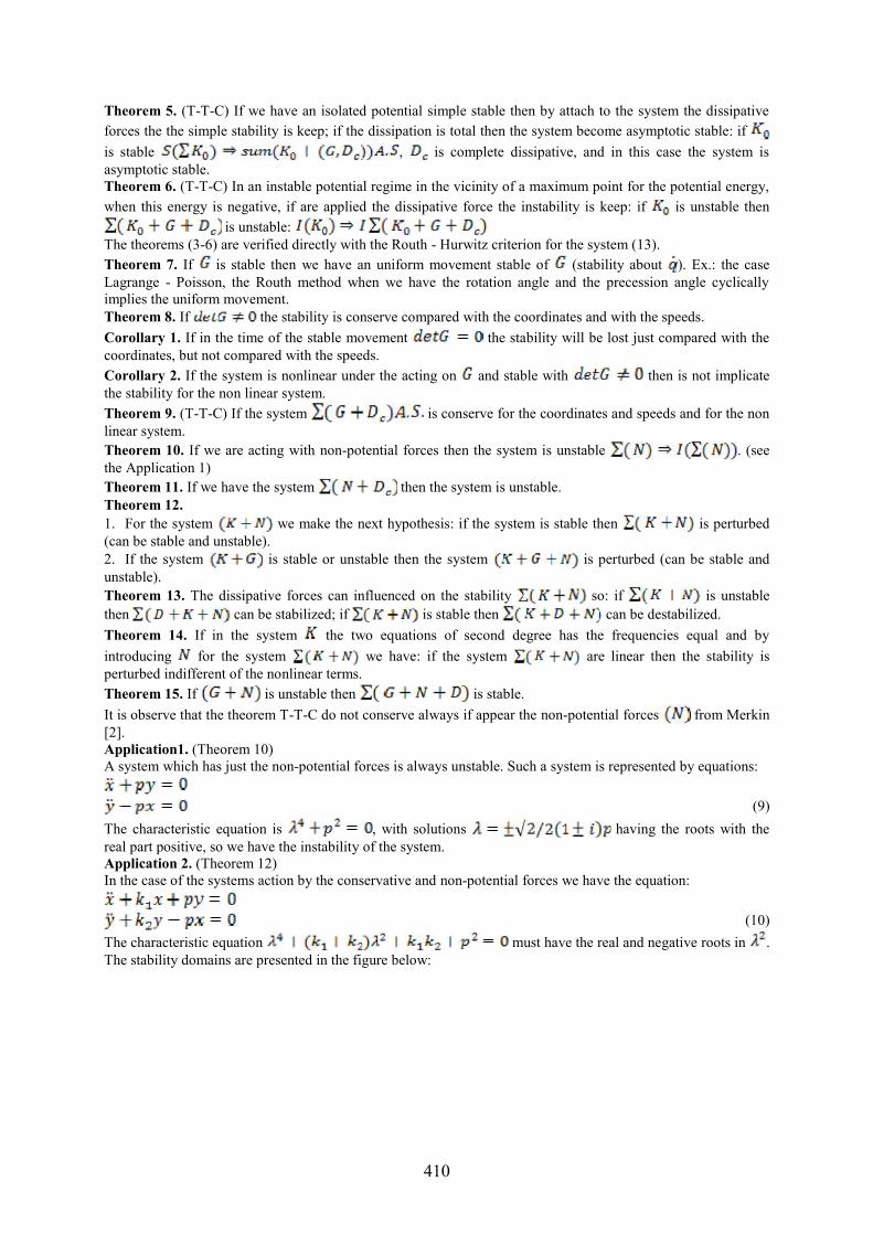
(9)The characteristic equation is , with solutions having the roots with thereal part positive, so we have the instability of the system.Application 2. (Theorem 12)In the case of the systems action by the conservative and non-potential forces we have the equation:

(10)The characteristic equation must have the real and negative roots in .The stability domains are presented in the figure below:

411

Figure 1: The domain of stability

Application 3. (Theorem 13)For the system action by the conservative and non potential forces, introducing the dissipative forces we have(fig. 1):

(11)The characteristic equation is:

Application 4. The gyroscopic pendulum with 2 degree of freedom and 2 types of amortization [1]:one linear stationary amortization and one rotational amortization withthe equations:

with the polar inertial momentum, the axial inertial momentum, the rotation speed, . Weobserve that the conservative forces are: the amortization forces

.From the theorem (Thomson - Tait - Cetaev)[3] the movement will be unstable being compose by a stablemovement and the other one unstable.The example of Crandall [3] shows that at the fast speed the movement is stable by using these amortizations,depend of the critical coefficient obtain a critical speed of amortization . On the other

side we observe the presence of the forces which introduce the unstable zones and stable zone from Merkinwhich do not conserve the theorem (T-T-C).Application 5. The cylindrical bearing with the rotor in the viscous fluid, with the center , [8]:The stability of the rotor centre [7]:

(12)

Here we have the forces: , where represents the aerodynamically forcesproduced by the rotor in the viscous fluid; the characteristic polynomial is:

(13)If then the stability domain is in the first quadrant. If then the stability is disappear, so the nonpotential forces ( ) can make the stability or can extend the stability (outside the first quadrant) (fig.1) [2].Application 6. The gyroscope with two plans [1], [2]There is keep the stability by the horizontal plan with angle and by the vertical plan with angle.

(14)

Using the Hurwitz criterion of stability we have:

For we have instability and for the system is asymptotic stable.

412

Application 7. The double pendulum with elastic articulations and a non-conservative force [3], [4], [5].The governing equation are:

(15)

For the asymptotic stability we have for the polynomial characteristic the conditions:

Application 8. The automobile with automatic decompression [4]

Figure 2: The stability of the automobile

The governing equations are:

(16)where is the inertial radius. For make the decompression of the two equations, to have a noiseless automobileit must: . This thing implies that (the gyration center) (fig. 2). In the figure 2cand 2d are decompose the movements in caper and gallop.Finally we present the indeterminate coefficients method, building Liapunov function for systems of forthdegree. The characteristic polynomial is:

(17)The H-R criterion for the S.A of the null solutions: .Next we’ll construct the Liapunov function for the system of 4thdegree. There are finding some functionswith four variables under the quadratic form:

(18)

where are unknown, are known; using the methods of undetermined coefficients, is derived for theattach system having four equations with the unknowns . In the algebraic linear system we have the

determinant, and we can choose and the identification . It is observe that, where , , . It is attach the

system:

here we choose to identify , so we have:

413

(19)

(20)For the nonlinear system we take the case when the term is replaced by :

(21)

(22)

We consider the case of a system with two freedom degree under the matricial form:(23)

where is the mass matrix, is the absorption matrix, is the potential elastic matrix.

(24)Passing at the system of fourth degree:

(25)The characteristic polynomial is:

(26)

By develop in series we obtain the polynomial of degree for which is appliying the theory above for find thefunction . Another applications of this kind regarding the stability study of the dynamical system and theirautomatic regulation are in the papers [5], [6], [7], [8], [9].

REFERENCES

[1] Dragos L., The principles of the analytical mechanics , Ed. Tech., Bucharest, 1976[2] Merkin D.R., Introduction in the movement stability theory, Moscova, Nauka, 1978[3] Stanescu N.D., Munteanu L., Chiroiu V., Pandrea N., Dynamical system Theory and Applications, Ed.Acad. Rom., Buc., 2007[4] Panovko Ya. G., Gubanova I.I., stability and oscilation in elastic systems, Ed. Moskva, 1964, (in russian)[5] Dumitrache I., The engineering of automatic regulation, Ed. Politehnica press, 2005, Bucharest[6] Chiriacescu S., Mechanical linear systems , Ed. Acad. Romane, Bucuresti, 2007.[7] Tanguy G.D., Fandloy L., Popescu D., Modelisation, identification et comandes des systems, Ed. Acad.Rom., 2004[8] Lupu M., Florea O. The study of the mass transfer in the case of the stationary movement of the viscousfluid between the cylindrical with parralel axis Proceedings of the International Conference, Acad. ForcesAeriene „Henri Coanda“, Brasov, 2007[9] Popescu D., Lupu. C, Pursuance systems in the industrial process Ed. Printech, 2004[10] Lupu M., Isaia F., The study of some nonlinear dynamical systems modelled by a more general Rayleigh -Van der Pole equation, J. Creative Mathematic and Inf., vol. 16/2007, pp 81-90