P2.2 QUALITY CONTROL OF A FUNDAMENTAL CLIMATE DATA RECORD FROM GEOSTATIONARY OBSERVATIONS:

CALIBRATION, NAVIGATION AND RADIOMETRIC QUALITY

Kenneth R. Knapp * NOAA National Climatic Data Center, Asheville, North Carolina

1. CLIMATE DATA RECORDS Efforts are underway to create climate data records from satellite data sets. Satellites have been recording reflected and emitted radiances for more than 20 years from both geostationary and low-Earth orbits. In particular, the Polar Operational Environmental Satellite (POES) and Geostationary Operational Environmental Satellite (GOES) operated by the National Oceanic and Atmospheric Administration (NOAA) have a long history of observations from consistent sensors. While the initial goal of these satellites was to observe weather, ocean and land, their extensive record provides an opportunity to analyze what the climate as well. In contemplating satellite climate data records (CDRs), an NRC committee delineated between fundamental and thematic CDRs. A fundamental climate data record (FCDR) is a quality-controlled time-series of sensor data which has undergone extensive testing and reprocessing to ensure consistency and monitor calibration for the entire record. Thematic climate data records (TCDRs) are geophysical variables derived from the FCDRs. The committee recommended that considerable effort be made to characterize the data in producing an FCDR. The High-resolution Infrared Radiation Sounders (HIRS) observation record represents a satellite-based observation record that may be considered to be an FCDR. Numerous studies attempt to understand the calibration of each of its channels. Also, much work has gone into understanding the effect of orbital-drift on the record. Yet aspects of the polar orbit – viewing an Earth location twice per day – limits the accuracy of TCDRs derived from this record which might be dependent upon diurnal changes. The geostationary orbit provides a different perspective – a fixed viewing geometry such that diurnal variations can be more readily observed and more accurately estimated. Thus, this work strives to characterize the geostationary record from the

* Corresponding author address: Kenneth Knapp; NCDC/RSAD; 151 Patton Ave.; Asheville, NC, 28801; email: Ken.Knapp@noaa.gov.

International Satellite Cloud Climatology Project (ISCCP) data set. 2. THE INTERNATIONAL SATELLITE CLOUD CLIMATOLOGY PROJECT ISCCP was designed as a federation of data providers (termed Satellite Processing Centers, SPC) which provide raw satellite data to the ISCCP Global Processing Center (GPC, located at the NASA/Goddard Institute for Space Studies). Figure 1 shows the data flow of the ISCCP processing. There are five satellite processing centers around the world which provide sampled geostationary data. Each SPC sub-samples the data to roughly 10 km and 3 hours – B1 data – and sends it to the NOAA/National Climatic Data Center (NCDC), which is the primary archive for the ISCCP. However, this data set was too large to be initially processed by the GPC, so each SPC performed a secondary sub-sampling to a spatial resolution of approximately 30km (B2 data). Each SPC also provides portions of the satellite imagery to the ISCCP Satellite Calibration Center (SCC) for use in satellite inter-comparisons to calibrate the observations, analyses of which are then provided to the GPC. Using this information, the GPC reformats and calibrates B2 data into B3 data which are used to perform the retrieval of cloud and surface parameters. One should note that B1 data are the only ISCCP data archived that are not used (i.e., processed) by the GPC, SCC or other satellite centers. At first this was due to the volume of the B1 data (in the context of the computing capabilities of the 1980s). But by the time computing power caught up with the B1 volume, the data set had already languished for years with little documentation and no support software. Thus, in light of the capability to process the entire B1 data set for climate research, it becomes necessary to assess and correct these deficiencies. Thus, work at NCDC is ongoing to compile B1 data documentation, develop input and output software, test data quality and make data accessible to the public.

3. ISCCP B1 DETAILS In spite of the fact that the ISCCP B1 data set is made up of different sensors on satellites launched by different countries, the observations are quite similar. The ISCCP data spans July 1, 1983 to present and is available at 3 hour intervals on the synoptic hour (00, 03, … 21 UTC). The start and end dates (along with primary location) is provided in Table 1. Yet while the temporal characteristics are rather uniform, the spatial and spectral details vary. 3.1 Spatial Characteristics

The primary strategy of the spatial sampling

was to create a data set which had a field-of-view about 5 km sampled to approximately 10 km. But due to the difference in spatial resolution, infrared channels were merely sampled, while visible channels were averaged then sampled (see Table 2 for details on the sampling). The visible channels were averaged to match the infrared spatial resolution then sampled in the same manner as an infrared (IR) pixel. In this way, the visible and IR radiances observe the same portion of the Earth. For instance, 8 8 visible pixel averaging was performed on the early GOES satellites to match the IR footprint, while the later GOES satellites have spatial averaging of 4 7 (due to along scan over-sampling in this series). Sampling of the averages is performed to keep them the same resolution as the IR sampling. Thus the spatial resolution of the B1 data set is centered near 8km with some above (primarily Meteosat and GMS) and other satellites with a lower resolution.

Also, it should be noted that while geostationary satellites can view a large portion of the Earth, their weakness is an inability to view the poles. Nonetheless when 5 GEO satellites are operating, 90% of the globe can be observed with a view zenith angle less than 75º. As such, when discussions herein mention global coverage, we mean continuity of coverage around the Equator (leaving observations of the remaining 10% of the Earth to polar-orbiting satellites).

The spatial coverage of the Earth is depicted in Figure 2. Most of the Earth is sampled for the entire span of the ISCCP record. The most prominent gap is the lack of satellite data over the Indian Ocean (from 55º to 85º East). However, with the move of Meteosat-5 to 63ºE in 1998, this gap was filled. This provides global coverage of the visible, infrared window and water vapor channels.

3.2 Spectral Characteristics The ISCCP B1 data is primarily composed of

visible, water vapor and infrared window channels (roughly, 0.6µm, 6.7µm and 11µm, respectively). The visible and infrared channels are window channels (i.e., most sensitive to surface, not the atmosphere) which help discriminate clouds from clear sky. Conversely, the water vapor channel is mostly opaque and as such, isn’t used in the ISCCP cloud mask algorithm. However, discussion of it is included here since it makes up a large part of the B1 data set and has been global in coverage since 1998. The relative similarity of the channels on all the satellites has allowed cross-calibration and has been used to estimate global cloud properties. The spectral responses (obtained from ISCCP sources) for each channel from all satellites are provided in Figure 3. The following is a discussion of similarities and differences in the spectral responses which may lead to discontinuities in the data.

The visible band is generally used to mask for clouds during the day. However, it has also been quantitatively used for surface insolation estimates, albedo retrievals and aerosol observations. Most visible bands (left column of graphs) have peak sensitivity near 0.7 µm. The entire GOES record and most of the GMS record show a full-width half maximum (FWHM) of approximately 0.5 to 0.7 µm, with the exception of GMS-5 which is 0.51 to 0.98 µm. The latter is more similar to the Meteosat record, which generally has FWHM of approximately 0.5 to 0.9µm. This makes the Meteosat series and GMS-5 more sensitive to water vapor variations (which absorbs at bands centered near 0.73, 0.83 and 0.93 µm).

The water vapor channels (Figure 3, center column) show two types of responses: narrow and broad bands. The narrow band responses, from 6.5 to 7.0µm, include GMS-5 (the first of the GMS series to have a water vapor channel) and GOES-8 through GOES-10. However, this narrow band limited the spatial resolution of the channel on the GOES series. With GOES-12, the band expanded to 5.7-7.3µm which measured more energy, allowing a spatial resolution identical to the other infrared channels. The response on GOES-12 is more similar to that measured by the Meteosat series.

Similarly, the channels near 11µm have broad and narrow bands. This time, though, the reason is due to the differences in atmospheric absorption between channels centered at 11 and 12 µm. Most

earlier satellites (early GOES, GMS and all Meteosat) have broad band centered near 11µm. This allowed the observation of the surface temperature. However, there is some water vapor absorption at these wavelengths. The Advanced Very High Resolution Radiometer (AVHRR) uses a split window method to remove the atmospheric transmittance by locating two narrow bands in the same region: one with less absorption (11µm) and the other with more atmospheric interference (12µm). The same approach was then incorporated on GOES-8 through 12 and GMS-5 with a narrow channel covering 10.2 to 11.2µm. Correspondingly, most of these also have a split window channel located at 11.5 to 12.5µm (not shown).

These channels represent the observations of ISCCP B1 data which are globally consistent (observations at other channels are available from satellites, for example, the near infrared channels of GOES-8 through 12, but their availability is limited). While differences between the channels described above do exist, their similarities have allowed cross calibration and geophysical retrievals which form the basis for the ISCCP cloud analysis. However, prior to performing geophysical retrievals using B1 data set, it should be analyzed to quantify sensor performance and document satellite-to-satellite biases or variations. 4. ISCCP B1 QUALITY CONTROL The important issues to consider to ensure accurate climate analysis from the B1 data are: quality control, navigation, and calibration. 4.1 Radiometric Quality The B1 data in their original form provide little information on data quality. In particular, analyses will be performed on each scan line (comparing them to surrounding scan lines) in an effort to remove noisy, missing or suspect data. This is the first step in quantifying data quality because it keeps corrupt data from interfering with further navigation and calibration tests. The details of this quality analysis are still being developed, but some tests will include removing:

• missing lines (where the standard deviation for the scan line is zero),

• duplicate scan lines, • corrupted scan lines (whose average or

standard deviation are not comparable to nearby scan lines), and

• temporal inconsistencies (where changes in time between adjacent scan lines are inconsistently large)

4.2 Navigation Quality Image navigation is crucial to satellite applications because it provides the geolocation of image pixels, determining such things as land or water classification and viewing/illumination geometry. Initially the satellites were spin-stabilized, but the newer GOES-8 series is 3-axis stabilized, each requiring different navigation algorithms. Among the spin-stabilized satellites, a variety of navigation styles were employed, including: Keplerian orbital elements, Chebyshev polynomials of the orbit, satellite position and velocity components, and rectification of the satellite image to a fixed view (as done for Meteosat). Navigation accuracy can be tested through comparisons with coincident imagery from other geostationary and polar satellites. Navigation tests are still being developed. In general, comparison between geostationary and AVHRR observations will be used to check for accuracy. The AVHRR observations are generally more accurately navigated and the infrared window can be used for tests during night or day. Also, tests will be calibration-independent because they will compare correlations between satellite digital counts, instead of calibrated temperatures. When AVHRR observations are not as available (such as when only one AVHRR was operational), nearby geostationary satellites can also be used. 4.3 Calibration Quality Calibration is perhaps the simplest of the B1 preprocessing steps, but the most important to quantify. The ISCCP processing includes a thorough cross-calibration between geostationary sensors as well as with AVHRR and HIRS (performed by the ISCCP Satellite Calibration Center). The B1 count values are identical in nature to those in the B3 data set (the only difference is spatial resolution). Thus the ISCCP B3 calibration tables can be used to calibrate B1 data. So tests will be applied to the calibrated ISCCP B1 data to analyze the results of the ISCCP calibration. An example of a preliminary calibration is provided below.

5. PRELIMINARY VISIBLE CALIBRATION Following (Rigollier et al. 2002) (hereafter,

R2002), a calibration equation for the conversion of the digital counts (DN) to reflectance, ρ, can be written: ρ = A(t) DN + B(t) (1) where A is the instrument response and B is an offset. Both vary in time since satellite responses tend to drift and will change between satellites. R2002 derive both A(t) and B(t) from time series of statistics of the full disk images. In short, the method assumes that the distribution of clear sky, land, and clouds remains invariant. The parameters of the probability distribution function (PDF) of a visible image can be used as a measure change in the sensor performance. The PDF is derived from imagery nearest the local noon hour to ensure the maximum illumination of the Earth. In this preliminary analysis, we focus on deriving A(t). From R2002, the instrument response is derived using:

( ) ( ) ( )( ) ( )

( ) ( )[ ]( ) ( )[ ]ooo

ooo

ttFttF

tDNtDNtt

tAθθρρ

coscos

580

580

−−

= (2)

where the first factor is representative of the instrument response, that is a change in ρ normalized by a change in DN. The subscripts refer to percentiles in the PDF. This calibration requires a known calibration on day to, such that the 5th and 80th percentiles of the reflectance can be calculated. The method assumes this difference is relatively constant in time, and can be related to corresponding changes in percentiles of the digital counts. Because the method is an assumption based on the PDF of reflectance viewed from a given location, it can be used for different satellites given the same satellite position. The second factor allows for changes in the instrument sensor, by normalizing about F, which is the total irradiance in the visible channel. It also allows for seasonal variation in the solar declination angle, by normalizing about the solar zenith angle (θo) at the sub satellite point. Equation 3 may be rearranged to form a constant and variable factor:

( ) ( ) ( )( ) ( )[ ]

( ) ( )[ ]( ) ( )

( ) ( ) ( )tVtCtAtDNtDN

ttFttFtt

tA

o

o

ooo

oo

=−

−=

580

580 coscos

θθρρ

(3)

Here, C(to) is the constant factor, and represents the calibration information from a day, to, on which the calibration is known. The variable portion, V(t),

is derived from the satellite observations on any particular day, t. The parameter V(t) is calculated for the ISCCP B1 data set from the observation closest to local noon for each satellite and shown in Figure 4. The plots are separated by satellite position and lines in each plot are linear regressions for each individual satellite (which can be determined from Table 1 or Figure 2). Overlaps are present because some satellites overlap in the coverage (notably, 0ºE in 1991 when MET-3, 4, and 5 were all active). In general, there are notable similarities and differences. The GOES series (at 75º and 135ºW) show numerous differences from the other satellite series. The values are much noisier, showing variations as large as 0.01 (note the noise from 1995-2005 at 135ºW). Also, more gaps are prevalent in the GOES data. This is due, in part, to the movement of GOES-6 and GOES-7 to the GOES-central location (at 100ºW) when other GOES satellites failed. Another factor is a data gap in the ISCCP B1 data, with 2 years of GOES-7 missing from 1992-1994 and 15 months of GOES-8 missing in 1996 and 1997. In spite of the gaps, the data for the GOES series show larger trends in the calibration than the other series. As mentioned earlier, the GMS-5 has a significant change in the spectral response of the visible sensor from the previous satellites in the series. This change is reflected in a change in the V(t) factor from 1995 to 2003. Given an accurate calibration, this effect, and others mentioned above, should be removed when looking at the C(t) factor. The invariant portion of A(t) is plotted in figure 5. C(t) is calculated using the calibrated reflectances, using ISCCP calibration tables. Since C(t) is calculated from calibrated visible reflectances, it should have a nearly constant value in time for each location. While some features described above remain, much has changed. For instance, the V(t) trends in the GOES series from 1995-2001 are now more constant. Also, the GMS-5 values are consistent with the previous satellites in the series, as well as GOES-9 which replaced it. This suggests that the ISCCP calibration coefficients were good, for the most part. However, work is needed to investigate any discrepancies. The factor C(t) shows less variation than V(t) in some areas, but shows a large discrepancy in September 2001. All satellites show a discrete change in C(t) in late 2001. At that time, the NOAA-16 AVHRR was introduced into the ISCCP processing. Since the geostationary satellites are

inter-calibrated using the AVHRR, it is likely that an error in the NOAA-16 calibration was passed to all the geostationary satellites. This is especially pronounced in satellites which were most consistent in their V(t) values. For example at 63ºE Meteosat-5 had low variability in V(t) but has a substantial change in C(t). Similarly, GOES-10 (135ºW) and GMS-5 (140ºE) both have consistent V(t) values, yet show a discontinuity at September 2001 in C(t). This suggests that a significant change in calibration (likely an error) was introduced in September 2001 and continues through the present. 6. SUMMARY AND FUTURE WORK

In summary, the B1 data set provides a unique

view of the earth, rich with climate information covering the past twenty years. With the ongoing work to test data quality, navigation and calibration, the B1 data can soon be used to develop long-term climate data sets for many atmospheric, land and ocean variables. The ISCCP B1 data provide information about the diurnal cycle not possible from polar-orbit. Thus, information from ISCCP B1 should be incorporated into future reanalysis of satellite data that produce climate data records. 7. REFERENCES

Rigollier, C., M. Lefevre, P. Blanc, and L. Wald, 2002: The Operational Calibration of Images Taken in the Visible Channel of the Meteosat Series of Satellites. Journal of Atmospheric and Oceanic Technology, 19, 1285-1293.

Table 1 – Details of ISCCP B1 data

Original Dynamic Resolution (bits) IR

Satellite Start Date End Date Meridian Missing (%) Vis

3.9µm 6.7µm 11µm 12µm GMS-1 01/21/1984 06/30/1984 135º E 6 6 8 GMS-2 07/01/1983 09/27/1984 135º E 17 6 8 GMS-3 09/28/1984 12/03/1989 135º E 7 6 8 GMS-4 12/04/1989 06/12/1995 135º E 1 6 8 GMS-5 06/13/1995 05/21/2003 135º E 1 6 8 8 8 GOES-5 07/03/1983 07/30/1984 75ºW 17 6 8 GOES-6 07/01/1983 01/19/1989 Variable 10 6 8 GOES-7 02/03/1987 01/11/1996 Variable 34(12)1 6 8 GOES-8 12/01/1994 04/01/2003 75º W 21(6)2 10 10 10 10 10 GOES-9 01/01/1996 07/27/1998 135º W 6 10 10 10 10 10 GOES-92 05/22/2003 Current 140ºE <1 10 10 10 10 10 GOES-10 07/28/1998 Current 135º W <1 10 10 10 10 10 GOES-12 04/01/2003 Current 75ºW <1 10 10 10 10 103 MET-2 08/31/1983 08/25/1988 0º W 14 8 8 8 MET-3 08/25/1988 06/19/1989 0º W 8 8 8 8 MET-34 09/12/1992 12/31/1994 60º W 11 8 8 8 MET-4 07/01/1989 02/03/1994 0º W 3 8 8 8 MET-5 02/03/1994 02/13/1997 0º W 1 8 8 8 MET-55 07/01/1998 Current 63º E <1 8 8 8 MET-6 02/13/1997 06/03/1998 0º W 1 8 8 8 MET-7 06/03/1998 Current 0º W 2 8 8 8 1 The number in parentheses represents the number of missing files when the missing files are replaced with data from the NCDC archive. 2 The GOES-9 satellite replaced the GMS-5. 3 The 13µm channel on GOES-12 replaced the 12µm split window channel. 4 The Meteosat-3 satellite was operating in Extended Atlantic data coverage. 5 The Meteosat-5 satellite was moved to 63º East longitude initially to provide data for the Indian Ocean Experiment (INDOEX), however it has remained there to fill in the gap in the geostationary coverage.

Table 2 – Spatial characteristics of the ISCCP B1 data set Satellite

Original IR Res. (km)

IR Sampling1

Nadir IR B1 Res (km)

Original Visible Res (km)

Visible Spatial Averaging1

Visible Sampling1

Nadir B1 Visible Res. (km)

GMS-1 5 2 2 10 1.25 4 4 2 10 10 GMS-2 5 2 2 10 1.25 4 4 2 10 10 GMS-3 5 2 2 10 1.25 4 4 2 10 10 GMS-4 5 2 2 10 1.25 4 4 2 10 10 GMS-5 5 2 2 10 1.25 4 4 2 10 10 GOES-5 7 1 22 7 0.9 8 8 1 7 7 GOES-6 7 1 2 7 0.9 8 8 1 7 7 GOES-7 7 1 2 7 0. 8 8 1 7 7 GOES-8 4 2 42 8 1 4 73 2 42 8 8 GOES-9 4 2 4 8 1 4 7 2 4 8 8 GOES-10 4 2 4 8 1 4 7 2 4 8 8 GOES-12 4 2 4 8 1 4 7 2 4 8 8 MET-2 5 2 2 10 2.5 2 2 10 10 MET-3 5 2 2 10 2.5 2 2 10 10 MET-4 5 2 2 10 2.5 2 2 10 10 MET-5 5 2 2 10 2.5 2 2 10 10 MET-6 5 2 2 10 2.5 2 2 10 10 MET-7 5 2 2 10 2.5 2 2 10 10 1 m n, where m is the number of scan lines and n is the number of pixels along the scan 2 Due to over sampling, IR pixels are under sampled in the along scan direction 3 Due to over sampling, this corresponds to a spatial resolution approximately 4 km 4 km

Figure 1 – Diagram depicting the primary function of the SPC (to provide B1 data to the archive and B2 data to the GPC). A subtle feature is that B1 data was archived but never used.

Satellite Processing Centers

ISCCP Central Archive

Global Processing Center

B3 (All satellites) Products (C,D Data)

B2

B2

GOES-5,6,7,8,9,10,12 Meteosat-2,3,4,5,6,7 GMS-1,2,3,4,5

NOAA-7,8, 9,10,11,12, 14,15,16,17

B1 GOES-5,6,7, 8,9,10,12 Meteosat-2,3, 4,5,6,7 GMS-1,2,3,4,5

Figure 2 – Spatial Coverage of the ISCCP geostationary satellites. Extent of the satellite coverage represents the 60º view zenith angle limit (sub-satellite point is represented by the gray lines)

Figure 3 – Spectral Responses of visible (left column), water vapor (center column) and infrared window (right column) channels from the ISCCP satellites.

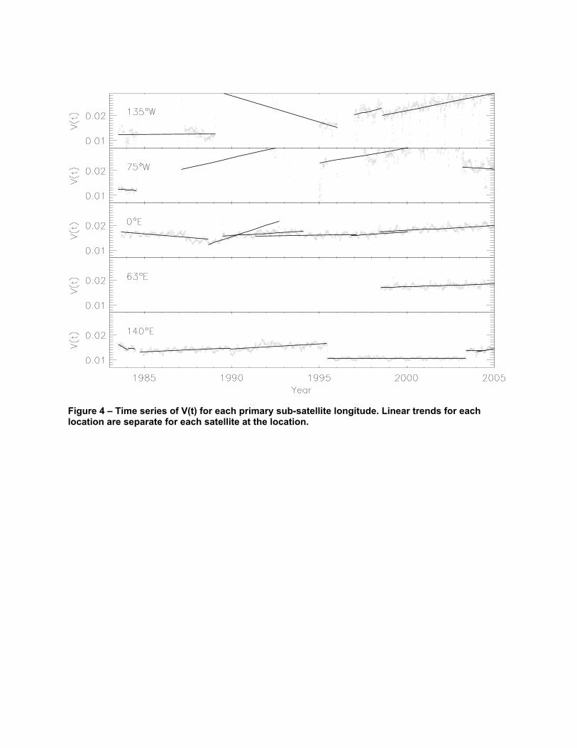
Figure 4 – Time series of V(t) for each primary sub-satellite longitude. Linear trends for each location are separate for each satellite at the location.

Figure 5 – C-1(t) (which should be constant) as a function of time for separate satellite locations (compare with figure 4). Separate solid lines indicate different satellites in a series. For satellites with data before and after Sept. 2001, linear trends of data before and after are shown. The vertical line represents September 2001, when a change in calibration likely occurred.