quality meshing of a forest of branching structures

Quality Meshing of a Forest of BranchingStructures

Chandrajit Bajaj1 and Andrew Gillette2

1 Department of Computer Sciences & Institute for Computational Engineeringand Sciences, University of Texas at Austin, USA [email protected]

2 Department of Mathematics & Institute for Computational Engineering andSciences, University of Texas at Austin, USA [email protected]

Abstract: Neurons are cellular compartments possessing branching morpholo-gies, with information processing functionality, and the ability to communicatewith each other via synaptic junctions (e.g. neurons come within less than anano-meter of each other in a specialized way). A collection of neurons in eachpart of the brain form a dense forest of such branching structures, with myr-iad inter-twined branches, inter-neuron synaptic connections, and a packingdensity that leaves only 5% - 10% volume fraction of exterior-cellular space.Small-scale variations in branching morphology of neurons and inter-neuronspacing can exert dramatically different electrical effects that are overlookedby models that treat dendrites as cylindrical compartments in one dimensionwith lumped parameters. In this paper, we address the problems of generat-ing topologically accurate and spatially realistic boundary element meshes ofa forest of neuronal membranes for analyzing their collective electrodynamicproperties through simulation. We provide a robust multi-surface reconstruc-tion and quality meshing solution for the forest of densely packed multiplebranched structures starting from a stack of segmented 2D serial sectionsfrom electron microscopy imaging. The entire 3D domain is about 8 cubic mi-crons, with inter-neuron spacing down to sub-nanometers, adding additionalcomplexity to the robust reconstruction and meshing problem.

1 Introduction

Biological modeling problems have long been an inspiration for geometry pro-cessing and meshing research. A relatively recent technique known as serialsection transmission electron microscopy (ssTEM) presents a new set of chal-lenges to the computational geometry community. The technique employs aCCD camera to capture high resolution images of parallel slices of a collec-tion of cells, usually neurons. The resolution on a single image slice is 5-10nanometers, small enough to identify features on the boundaries of the cells,

2 Chandrajit Bajaj and Andrew Gillette

Fig. 1. Neuronal modeling from imaging uses serial section transmission electronmicroscopy (ssTEM), producing a stack of image slices. [18, 36] The imaging data iscourtesy of Dr. Kristen Harris from the Section of Neurobiology at UT Austin. Onthe left, a single slice is shown with contours representing cell boundaries shown inred. The contours are tagged based on the neuronal process they belong to - purplefor dendrites, green for axons, yellow for glial - as shown on the right. The taggedcontours are used for accurate surface reconstruction, such as the purple dendritemodel shown here, so that surface area, volume, and other properties of the cellscan be calculated.

as well as organelles within the cells. [18, 36] Trained neuro-anatomy awareusers can approximate the cell boundaries by visual inspection and label theirpolygonal contours consistently through the stack so that slice images of a sin-gle cell (dendrite, glial, axon, etc.) can be traced through the entire volume,as shown in Figure 1. This suggests the following computational problem:develop a method to create a watertight mesh of a multi-component, com-pact 2-manifold passing through the labeled boundaries on each slice withbiologically-accurate topology and spatially-accurate geometry. A sample ofmeshes created by our lab solving this problem are shown in Figure 2. Themeshes will be used to research quantitative morphology [21] and to calibratetime-dependent electrophysiological simulation of voltage potentials [33]. Wediscuss this further in Section 5.

The unique challenge in processing and modeling neuronal cell data is themulti-component nature of the problem. Reconstruction of a single compo-nent surface from 2D slices has been heavily researched in recent decades. Aseminal paper in this vein is the work of Fuchs, Kedem, and Uselton [22] whichfocused on triangulating a stack of polygonal contours using a toroidal graphto guide construction. Christiansen and Sederberg [15] helped to characterizethe branching problem and potentially ambiguous situations that may arise.Meyers, Skinner and Sloan [32] identified the subproblems of correspondence,tiling, branching and surface-fitting and gave a resolution based on a mini-mum spanning tree. Barequet and Sharir [7] developed an algorithm focusedon medical applications such as Computerized Tomography (CT) and Mag-netic Resonance Imaging (MRI); this was expanded upon by Bajaj, Coyleand Lin [4] who introduced the use of the medial axis to aid in topologically

Quality Meshing of a Forest of Branching Structures 3

accurate surface meshing. Similar approaches used the Voronoi diagram [34]or a discrete distance function [28] to guide reconstruction. Barequet et al. [6]have also used the straight skeleton to aid in the case of nested contours. Re-lated to these surface meshing approaches are techniques for volume meshing[9, 24, 14], non-linear surface fitting [11, 27, 37, 8], and recently non-parallelplane methods [10, 31].

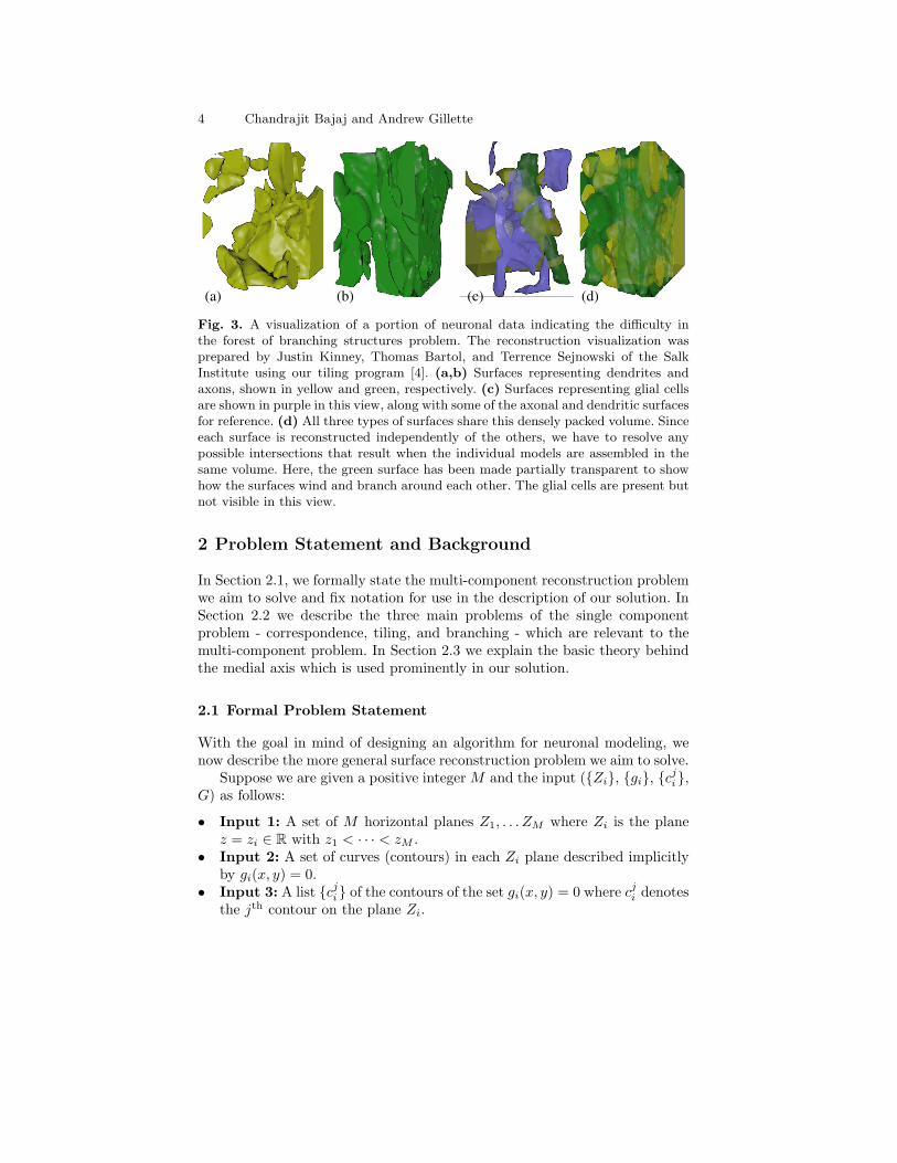
Unfortunately, resolving the multi-component problem by separating itinto independent single-component problems is not sufficient to guaranteean appropriate solution for neuronal models. Image data reveals that neuronshave widely varying cross-sectional areas and boundary shapes and are packedvery densely (an example is shown in Figure 3), with as little as 5-10% of theimage representing extra-cellular space [26, 35]. Even if the contours approxi-mating the boundaries on each slice are non-overlapping, an under-constrainedsurface reconstruction might create intersections in three dimensions.

(a) (b)

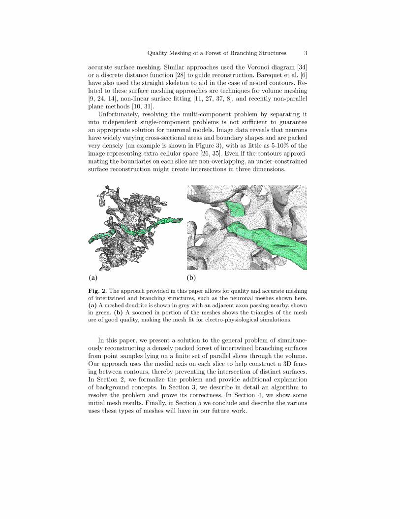
Fig. 2. The approach provided in this paper allows for quality and accurate meshingof intertwined and branching structures, such as the neuronal meshes shown here.(a) A meshed dendrite is shown in grey with an adjacent axon passing nearby, shownin green. (b) A zoomed in portion of the meshes shows the triangles of the meshare of good quality, making the mesh fit for electro-physiological simulations.

In this paper, we present a solution to the general problem of simultane-ously reconstructing a densely packed forest of intertwined branching surfacesfrom point samples lying on a finite set of parallel slices through the volume.Our approach uses the medial axis on each slice to help construct a 3D fenc-ing between contours, thereby preventing the intersection of distinct surfaces.In Section 2, we formalize the problem and provide additional explanationof background concepts. In Section 3, we describe in detail an algorithm toresolve the problem and prove its correctness. In Section 4, we show someinitial mesh results. Finally, in Section 5 we conclude and describe the varioususes these types of meshes will have in our future work.


(b) (c) (d)(a)

Fig. 3. A visualization of a portion of neuronal data indicating the difficulty inthe forest of branching structures problem. The reconstruction visualization wasprepared by Justin Kinney, Thomas Bartol, and Terrence Sejnowski of the SalkInstitute using our tiling program [4]. (a,b) Surfaces representing dendrites andaxons, shown in yellow and green, respectively. (c) Surfaces representing glial cellsare shown in purple in this view, along with some of the axonal and dendritic surfacesfor reference. (d) All three types of surfaces share this densely packed volume. Sinceeach surface is reconstructed independently of the others, we have to resolve anypossible intersections that result when the individual models are assembled in thesame volume. Here, the green surface has been made partially transparent to showhow the surfaces wind and branch around each other. The glial cells are present butnot visible in this view.

2 Problem Statement and Background

In Section 2.1, we formally state the multi-component reconstruction problemwe aim to solve and fix notation for use in the description of our solution. InSection 2.2 we describe the three main problems of the single componentproblem - correspondence, tiling, and branching - which are relevant to themulti-component problem. In Section 2.3 we explain the basic theory behindthe medial axis which is used prominently in our solution.

2.1 Formal Problem Statement

With the goal in mind of designing an algorithm for neuronal modeling, wenow describe the more general surface reconstruction problem we aim to solve.

Suppose we are given a positive integer M and the input ({Zi}, {gi}, {cji},

G) as follows:

• Input 1: A set of M horizontal planes Z1, . . . ZM where Zi is the planez = zi ∈ R with z1 < · · · < zM .

• Input 2: A set of curves (contours) in each Zi plane described implicitlyby gi(x, y) = 0.

• Input 3: A list {cji} of the contours of the set gi(x, y) = 0 where cj

i denotesthe jth contour on the plane Zi.


• Input 4: A directed graph G with vertices⋃

i,j cji and edges only pointing

to an element of list index incremented by one. That is, every edge of Gcan be written as (cj1

i , cj2i+1) for some indices i, j1, and j2.

Our goal is to construct a smooth function g : R3 → R such that the followingproperties hold:

• Property 1: The surface g(x, y, z) = 0 is a compact 2-manifold.• Property 2: The function g restricts to gi on Zi. That is, for all i,

g(x, y, zi) = gi(x, y) for all (x, y) ∈ R2.• Property 3: The surface g(x, y, z) = 0 has local connectivity correspond-

ing to the graph G. That is, if (cj1i , cj2

i+1) is an edge in G, then cj1i and

cj2i+1 are homologous (meaning one smoothly deforms into the other) on

the surface{(x, y, z) : g(x, y, z) = 0, z ∈ [zi, zi+1]}

We note that the set {g−1(0)} is the desired surface passing through thecontours with the correct connectivity. A general analytical solution to thisproblem is difficult and unnecessary for implementation, hence we make thefollowing simplifying assumptions based on the application context.

Definition 1 (adapted from [1]) A homeomorphism h of R3 is isotopic tothe identity if there is a homotopy H : R3 × [0, 1] → R3 such that for eacht ∈ [0, 1], ht := H(·, t) : R3 → R3 is a homeomorphism, h0 is the identity andh1 = h. A mesh M ⊂ R3 of a surface S ⊂ R3 is called an isotopic meshif and only if there exists a homeomorphism h of R3 carrying M to S with hisotopic to the identity.

• Assumption 1: The contours are described by simple polygons whosevertices lie on the contour. If the geometry of a particular polygon needsto be refined, the appropriate gi can be referenced to increase the samplingdensity.

• Assumption 2: If M is a compact piecewise linear 2-manifold such thatit restricts to the contours on each slice and has local connectivity cor-responding to the graph G, then M is an isotopic mesh of the surfaceg(x, y, z) = 0.

• Assumption 3: The distance between consecutive zi values is smallenough that the slice sampling of each component in the surface g(x, y, z) =0 meets the requirements of the single-component meshing algorithm.

Each assumption is based on practical considerations from neuronal data.To satisfy Assumption 1, we fit each polygonal contour data as tagged bybiologists with a regular algebraic spline curve called an A-spline. By usingthe error-bounded spline method described in [5], we can construct smoothapproximations of the contours while preventing overlaps between adjacentcontours. The splines are defined locally based on a scaffolding mesh, allow-ing us to efficiently increase the sampling of a contour in a particular region


if needed. Assumption 2 is made to distinguish the surface meshing problemfrom the smooth surface construction problem. In this paper, we are onlyinterested in how to create an isotopic mesh of the smooth surface approxi-mation and leave the surface fitting to future work. Assumption 3 is stated sothat we can tackle the multi-component problem without inheriting existingdifficulties from the single component problem. As is discussed in [4], it isdesirable to produce a mesh such that any vertical line between two adjacentslices passes through the mesh at most once. We clarify this criterion in thenext subsection.

2.2 Correspondence, Tiling, and Branching

The single component surface reconstruction problem faces three major sub-problems: the correspondence problem, the tiling problem and the branchingproblem. Our solution to the multi-component problem requires an effectivesingle component solver, hence we will review the three problem types here.The single component solver we use is denoted SingleSurfRecon and re-solves the problems in full generality under the assumptions previously stated.The method is summarized below, but is given in full detail in [4]. To describethe problems, we consider two planes Z1 and Z2 with z1 < z2 and let {cj

1},{ck

2} denote the lists of contours in the respective planes. Figure 4 illustratessome of the difficulties in meshing such intricate data.

(a) (b)

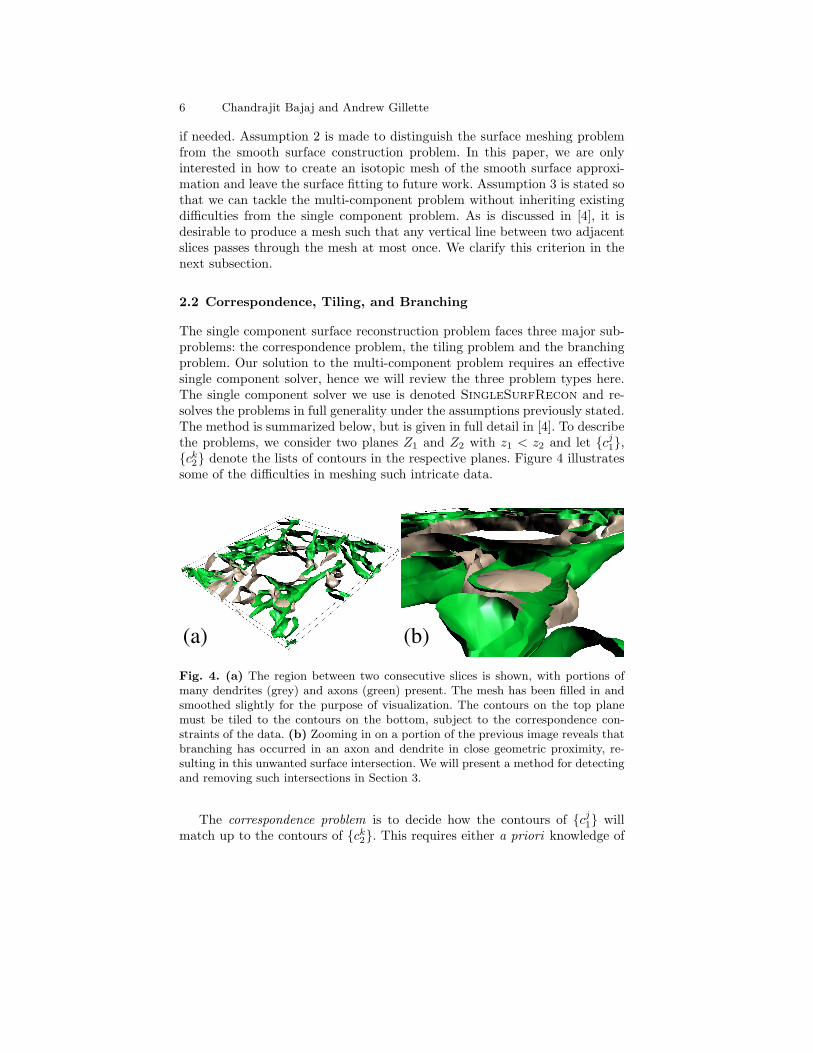
Fig. 4. (a) The region between two consecutive slices is shown, with portions ofmany dendrites (grey) and axons (green) present. The mesh has been filled in andsmoothed slightly for the purpose of visualization. The contours on the top planemust be tiled to the contours on the bottom, subject to the correspondence con-straints of the data. (b) Zooming in on a portion of the previous image reveals thatbranching has occurred in an axon and dendrite in close geometric proximity, re-sulting in this unwanted surface intersection. We will present a method for detectingand removing such intersections in Section 3.

The correspondence problem is to decide how the contours of {cj1} will

match up to the contours of {ck2}. This requires either a priori knowledge of


the contours’ connectivity or a geometric criterion for declaring correspon-dence. In the context of our problem domain, the correspondence problem forSingleSurfRecon is resolved by consulting the graph G as it prescribes theconnectivity between contours.

The tiling problem is to decide, given contours c1 ∈ {cj1} and c2 ∈ {ck

2},how c1 and c2 will be joined in the interslice region. In the context of meshing,c1 and c2 are given as polygons and the problem is to decide how to addedges between them so that a suitable mesh of the ribbon surface betweenthe contours is produced. A line segment connecting c1 to c2 is called a slicechord and a triangle formed by two slice chords an edge of a contour is calleda tiling triangle. Even in very simple cases, there are many choices availablefor how to choose slice chords and tiling triangles. One resolution to thisproblem is to define a quality measure on possible tilings and seek a tilingwith the optimal quality [22, 15]. A summary of different quality metrics usedin early methods is given in [32]. Alternative approaches, such as the one weuse, project contours from Z2 to Z1 and use planar geometry properties tolift a watertight surface mesh from the projection [4, 34, 28, 6].

The choice of tiling method is highly relevant to the types of guaranteesone can provide on the output meshes. We have selected the method of [4]because it only outputs surfaces that meet the following three criteria.

• Criterion 1: The reconstructed surface forms a piecewise closed surfaceof polyhedra.

• Criterion 2: Any vertical (meaning parallel to the z axis) line segmentbetween two adjacent slices intersecting the reconstructed surface does soat exactly one point or along exactly one line segment.

• Criterion 3: Resampling of the reconstructed surface on any slice repro-duces the original contours.

Criterion 1 ensures that self-intersecting surfaces and other incorrect meshesare not formed. Criterion 3 ensures that all the contours are interpolated andno new ones are created. Criterion 2 is especially important because it ensuresthat the reconstructed surface is functional from its nearest planes. That is,barring the case of vertical surface patches, the projection of any trianglein the mesh to either of its two nearest Zi planes is a one-to-one mapping.This prevents unlikely topologies from being formed and aids in the proofof the correctness of the multi-component method as discussed in Section3.7. We note that Criterion 2 may not be satisfiable if the distance betweenconsecutive zi values is too large relative to the surface feature size, however,by Assumption 3, this is not the case. In practice, exceptions to Assumption3 are rare and therefore Criterion 2 is not particularly restrictive on the inputtype.

We will now summarize the approach that the SingleSurfRecon algo-rithm uses to resolve the tiling problem. We will appeal to intuitive notionsof the left side and right side of a vertex on a contour relative to its clockwise(CW) or counterclockwise (CCW) orientation; these definitions are made ex-


plicit in [4]. Let {ck2′} denote the projection of {ck

2} vertically onto Z1. Wecompute the points of intersection between {cj

1} and {ck2′}; without loss of

generality we assume that these points of intersection are vertices on contoursin both sets. Such vertices that are common to both sets are called an overlap-ping vertices; all other vertices are called non-overlapping. If a tiling of {cj

1}and {ck

2} satisfies the three Criteria, the following two theorems must hold.

Theorem 1. ([4], Theorem 2) Let v be a vertex on a contour in c1 ∈ {cj1}

and T a slice chord from v. (i) If v is a non-overlapping vertex, the projectionof T onto Z1 is contained entirely on one side (right or left) of c1. The sideis determined by the orientation of the nearest enclosing contour from the set{ck

2} when v is projected to Z2. (ii) If v is an overlapping vertex, v also belongsto some c′2 ∈ {ck

2′} by hypothesis. In this case, the projection of T onto Z1

does not intersect the region to the left of both c1 and c′2 at v, nor the regionto the right of both c1 and c′2 at v.

Theorem 2. ([4], Theorem 4) Let T be a slice chord and c1 ∈ {cj1}. Then the

projection of T onto Z1 cannot intersect both the inside and outside of c1

The tiling algorithm proceeds as follows. For each vertex v ∈ {cj1}, make

a list of all the slice chords that could be formed to a vertex of {ck2} (based

on the resolution of the correspondence problem). Select the shortest lengthchord from this list which satisfies the results of Theorems 1 and 2. If nochord from the list satisfies both Theorems, tag the vertex as “untiled.” Theboundaries of untiled regions are later collected and meshed separately whileresolving the branching problem.

The branching problem arises when the result of the correspondence prob-lem yields a matching of more than one contour in {cj

1} to any number of con-tours in {ck

2} (or vice versa). Solutions to the problem include adding edges tothe contours on one of the planes or adding vertices in between the planes tocreate an appropriate mesh. Since the former approach violates Criterion 3,we employ the latter. The branching problem occurs only in regions previouslytagged as “untiled” by SingleSurfRecon, so we collect the boundaries ofthese regions and project them to a plane half way between the two planesin consideration. We triangulate these untiled regions based on their EdgeVoronoi Diagram using the algorithm of Lee [29]. Any new vertices added aregiven a z value of .5(z1 + z2). A summary of alternative approaches to thebranching problem and further details are given in [4].

The output of SingleSurfRecon is a mesh with the desired Propertiesand satisfying the given Criteria. In practice, SingleSurfRecon can be im-plemented in a numerically stable manner and will provide an output for manytypes of real data.

2.3 Medial Axis

The main tool employed by our algorithm to ensure accurate surface recon-struction is the medial axis of the region exterior to the contours. We give a


Fig. 5. A collection of contours representing cell boundaries and their interiors areshown in red along with the approximate medial axis of intracellular space MP

shown in blue.

thorough explanation of the medial axis in Appendix A. The medial axis ofa set O is often approximated based on a point sampling P of the boundary∂O and the Voronoi and Delaunay diagrams Vor P and Del P . A definitionof these diagrams and how to compute them can be found in any standardcomputational geometry textbook, e.g. [19]. The medial axis is approximatedby the graph of the vertices of Vor P along with those edges of Vor P notintersecting the contours. We denote this graph MP ; an example is shownin Figure 5. For 2D cellular contour data, MP will have one component foreach cell interior plus a component for the extracellular region, assuming Pis a sufficiently dense sampling of ∂O. We discuss sampling density and ourrobust medial axis computation method further in Section 3.2.

3 Algorithm

In this section we describe an algorithm to solve the multi-component problemunder the Assumptions given in Section 2.1. In the next six subsections, wewill explain the input to the algorithm and its five major steps. We concludethis section with a proof of the correctness of the approach.

3.1 Algorithm input

As stated in Section 2.1, our input is the following objects: ({Zi}, {gi}, {cji},

G). By our stated Assumptions, we may suppose that the contours {cji} are

simple polygons with sufficiently dense sampling of the level sets gi(x, y) = 0.Define Pi = {v : ∃j such that v is a vertex on cj

i}. We pass these polygonalcontours and the associated point sets Pi to our algorithm instead of thefunctions gi.

For ease of description and to maintain consistency with our neuronal data,we explain the algorithm for the case where G has just two components, with


one colored yellow and one colored green. Each contour can thus be uniquelyassigned as belonging to the set of yellow contours Y C or green contours GC,i.e.

{cji} = Y C

∐GC

The notation we will use for calling the algorithm with this input is

MultiSurfRecon({Zi},

{cji

}, {Pi}, G

)3.2 Step 1: Construct and partition 2D medial axes

Overview

Compute the approximated medial axis MPi for each 1 ≤ i ≤ M and discardthe portions interior to the contours. Each remaining edge e separates twounique contours, call them ce1 and ce2. Partition these edges into three sets:

EY Y = {e : ce1, ce2 ∈ Y C}, EGG = {e : ce1, ce2 ∈ GC},

EGY = {e : ce1 ∈ Y C, ce2 ∈ GC or ce1 ∈ GC, ce2 ∈ Y C}

Details

It is crucial that the medial axes on each slice be computed robustly and withtopological accuracy for the remainder of the algorithm to work. Thus, weturn to a criterion established by Edelsbrunner and Shah known as the closedball property [20] which we state here for polygonal contours in a plane. LetP be the vertices of all the contours and Σ the union of all the contours on aparticular plane. A Voronoi object V from Vor P of dimension k satisfies theclosed ball property if and only if V ∩Σ = ∅ or V ∩Σ is homeomorphic to aclosed ball of dimension k−1. If all V ∈ Vor P satisfy the closed ball propertyand Σ intersects each V transversally, then Σ is a subgraph of Del P [20].This implies that MP is a subgraph of Vor P . Cheng, Dey, Ramos, and Rayused this criterion to create Delaunay-conforming meshes without approxi-mating local feature size [13]. We provided an efficient algorithm exploitingtheir approach for use with image data [25] and we adopt that algorithm forcomputation of MP . Figure 5 shows a zoomed in picture of a slice of extractedcontours with MP displayed.

By construction, MP is a multi-component piecewise linear graph. Wediscard all components of MP which are interior to the contours, leaving asingle medial axis approximation of extracellular space. From this point on,we will take MP to mean this single connected graph. Each edge of MP is aVoronoi edge and thus its dual Delaunay edge connects two points of P . Weassign each edge to EGG, EY Y , or EGY based on whether its associated pointsof P are both on green contours, yellow contours, or one of each, respectively.


3.3 Step 2: Construct medial surface

Overview

Dilate the edges in EGY so that they form contours and color these con-tours red. Run SingleSurfRecon on the red contours, producing a partial,approximate medial surface MS.

Details

On each plane, we consider only those edges of MP which belong to EGY .We dilate EGY by setting a distance parameter ε and defining the contoursto be the locus of points at distance ε from EGY . For small enough valuesof ε, this produces a collection of contours to which we assign the color red.We denote the dilated contours RC. Once we have done this for all the slices,we call SingleSurfRecon on the whole set RC to produce a partial medialsurface approximation denoted MS. In this computation, we also computethe intersection of MS with each intermediate plane z = .5(zi + zi+1).

3.4 Step 3: Create single component surfaces

Run SingleSurfRecon on Y C and GC separately, producing meshes of theyellow and green contours. In this run, we also keep a list of those i values forwhich vertices were added on the intermediate plane z = .5(zi + zi+1). Thisoccurs whenever there are dissimilar contours or branching in a portion of thetiling.

3.5 Step 4: Remove overlaps on intermediate planes

Overview

For those i values on the list created in Step 3, compute the yellow, green, andred contours that occur on plane z = .5(zi + zi+1), which we denote Zi,i+1.Do a plane sweep to detect overlaps between contours and remove them sothat the mesh now avoids overlaps on each intermediate plane. Output themodified meshes of Y C and GC.

Details

From Steps 2 and 3, we have calculated red, yellow, and green contours on eachintermediate plane Zi,i+1. Geometrical problems may arise on those Zi,i+1

planes which have yellow and/or green vertices. For those planes, we do aplane sweep to detect overlap regions. We distinguish between two types ofoverlaps: simple transversal overlaps and exotic overlaps. A simple transversaloverlap is one in which the border of the region is exactly two colors andeach of these colors forms a connected component of the border. We resolve


simple transversal overlaps by first computing the medial axis associated tothe interior of the overlap. This is then used as a dividing line to guide vertexmovement; the overlap is resolved by moving each vertex on the boundaryacross this axis. Note that this method does not add or remove vertices, doesnot change the mesh connectivity, and does not change the z value of anyvertex.

(c)(b)(a)

Fig. 6. (a) A few overlaps have occurred on an intermediate plane Zi,i+1 betweengreen contours, yellow contours, and red medial surface contours. We attempt toresolve them by searching for simple transversal overlaps such as the green/yellowoverlap in this case. (b) After removing the green/yellow overlap, we are left withonly red/yellow and red/green overlaps. (c) Removing the final overlaps, all thecontours are separated.

zi+1

zi,i+1

(a) (b) (c) (d)

zi

Fig. 7. A toy example of how our algorithm works in the case of exotic overlaps (seeSection 3.5). (a) Green and yellow contours are detected in adjacent planes Zi, Zi+1

and the medial axis MP in each plane is computed, shown in red. Those portionsof the medial axis which lie between same color contours are discarded, such as thedashed red portion in the upper plane. (b) An approximate medial surface MS iscomputed by dilating the MP into contours and calling SingleSurfRecon. Theintersection of MS and the separately computed green and yellow surfaces with theintermediate plane Zi,i+1 is shown. The overlap of the contours cannot be resolvedby removing simple transversal overlaps. (c) To remove the overlap, we move thegreen vertices on Zi,i+1 to a lower z value and the yellow vertices to a higher z value,without changing connectivity of the mesh. We show the intersections of the yellowand green surfaces on the two intermediate planes where the vertices have beenmoved. (d) The skeletons of the yellow and green meshes are shown to illustratethat the overall topology is now correct and no geometrical overlaps occur.


An exotic overlap in a region Q can often be resolved by finding simpletransversal overlaps within Q and resolving them in the manner describedabove. Such a case is shown in Figure 6. If this is not possible, we resolve theexotic overlap by changing the z values of vertices in the overlap region toeither .25(zi + zi+1) or .75(zi + zi+1). An example of such a case and how itis resolved is shown in Figure 7.

3.6 Step 5: Quality improvement

We decimate and improve the quality of our output meshes in the followingmanner. For decimation, we first do edge contractions based on the Delau-nay diagram, using the QSlim software by Michael Garland [23]. We then donormal-based triangle decimation based on the method presented in [3]. Fi-nally, we improve the shape of triangles in the mesh using a geometric flowtechnique [38] which is a library in Level Set Boundary Interior and Exte-rior Mesher (LBIE) [16], part of the Volume Rover (VolRover) [17] softwaredeveloped by our lab.

3.7 Correctness of the Algorithm

The goal of MultiSurfRecon is to output an isotopic mesh M of the multi-component surface S representing neuronal membranes such that the Haus-dorff distance between M and S is small. Since SingleSurfRecon producessuch meshes for individual components, the main question is whether theunioning and separating processes employed by MultiSurfRecon truly re-move all intersections between the component surfaces in three dimensions.We will show that removing mesh intersections on certain horizontal planessuffices to preclude any 3D intersections in the complete mesh. To state thismore precisely, we introduce the following definitions and lemmas.

Definition 2 • An original contour is any contour cji from Input 3 (de-

scribed in Section 2.1). By Assumption 1, each cji is a simple polygon.

• A branching point is a vertex added by MultiSurfRecon whose z-value is not one of the zi values from Input 1.

• An intermediate plane is a horizontal plane which, after running Mul-tiSurfRecon, contains at least one branching point.

• The branching set of a mesh component C on an intermediate plane Pis the collection of branching points on P which belong to C, along withany edges of C between these points.

• An intermediate contour is a contour formed by intersecting M withan intermediate plane P . Note that an intermediate contour may containsome of the branching set of the component in which the contour lies.

• Let c1, c2 be contours in the same plane and I(c1), I(c2) their respectiveinteriors. Then c1 and c2 are said to overlap if and only if (I(c1)∪ c1)∩c2 6= ∅ and (I(c2) ∪ c2) ∩ c1 6= ∅. Note that if one contour is completelycontained in the other, they do not overlap.


Lemma 1. Suppose that for each i, there are no pairwise overlaps betweenthe original contours on plane Zi. Then the output of SingleSurfReconrun on any subset of the original contours is not self-intersecting.

Lemma 1 is a consequence of the three Criteria laid out in Section 2.1 andthe tiling method; if the original contours do not overlap, SingleSurfReconcannot create self-intersections.

Next, observe that for the output of MultiSurfRecon with componentsY C and GC, there are three types of overlap that may occur on an interme-diate plane P :

• An intermediate contour of Y C intersects an intermediate contour of GC.• An intermediate contour of Y C intersects the branching set of GC (or vice

versa).• The branching sets of Y C and GC intersect.

This characterization of types of overlaps extends naturally to outputs withmore than two components. The following lemma shows that detecting andremoving these types of overlaps is equivalent to removing self-intersectionsof the entire mesh. The lemma makes use of Assumption 2 from Section 2.1,without which, problems could arise from contours on consecutive planes beingnested inside each other in contradictory ways. Since this should not happenwith real data, we feel we are justified with the Assumption as stated.

Lemma 2. If there are no overlaps of any of the three types on any interme-diate plane, then the output of MultiSurfRecon has no self-intersectionsin the entire volume. Conversely, if the output has no self-intersections in thevolume, it does not have any overlap on any intermediate plane.

Proof. For the forward direction, consider the stack of all the original andintermediate planes in the output. By hypothesis, there are no overlaps andhence no surface intersections on any of these planes. Further, between anypair of consecutive planes there are no branching problems, as otherwise theplanes would not be consecutive in the stack. Therefore, the surface betweenconsecutive planes is a linear interpolation of the contours by Criterion 2from Section 2.2. By Assumption 2 from Section 2.1, the true surface is a 2-manifold in this region meaning the linear interpolation is not self-intersecting.Therefore, the entire output is not self-intersecting. For the converse, if theoutput is not self-intersecting, the components do not intersect each other andtherefore do not overlap on any intermediate plane. ut

By Lemma 2, the removal of simple transversal and exotic overlaps donein Step 4 of the algorithm suffices to separate the components of the forest ofbranched surfaces in the entire volume. In future work, we plan to examinewhether knowing the type of overlap on an intermediate plane can be used tosimplify the procedure of Step 4.


4 Implementation and Results

(a) (b)

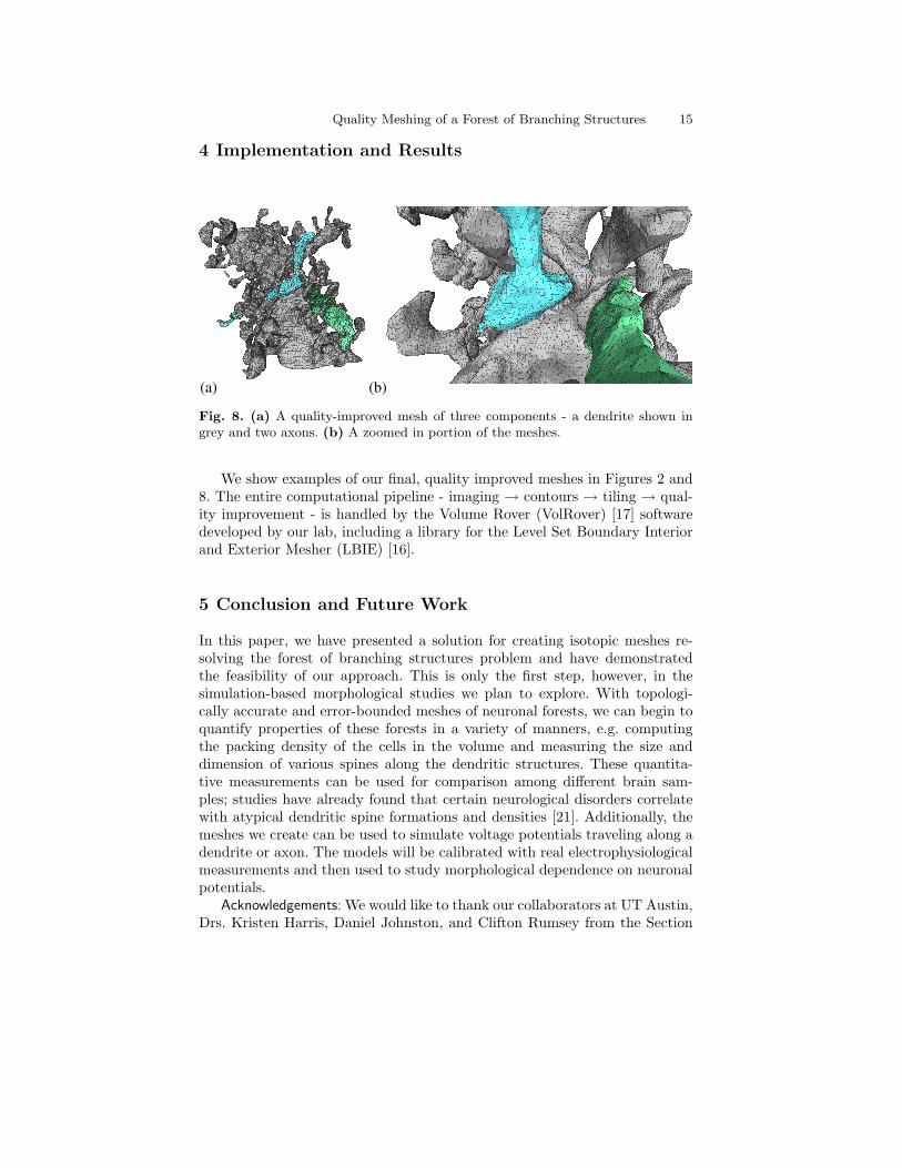
Fig. 8. (a) A quality-improved mesh of three components - a dendrite shown ingrey and two axons. (b) A zoomed in portion of the meshes.

We show examples of our final, quality improved meshes in Figures 2 and8. The entire computational pipeline - imaging → contours → tiling → qual-ity improvement - is handled by the Volume Rover (VolRover) [17] softwaredeveloped by our lab, including a library for the Level Set Boundary Interiorand Exterior Mesher (LBIE) [16].

5 Conclusion and Future Work

In this paper, we have presented a solution for creating isotopic meshes re-solving the forest of branching structures problem and have demonstratedthe feasibility of our approach. This is only the first step, however, in thesimulation-based morphological studies we plan to explore. With topologi-cally accurate and error-bounded meshes of neuronal forests, we can begin toquantify properties of these forests in a variety of manners, e.g. computingthe packing density of the cells in the volume and measuring the size anddimension of various spines along the dendritic structures. These quantita-tive measurements can be used for comparison among different brain sam-ples; studies have already found that certain neurological disorders correlatewith atypical dendritic spine formations and densities [21]. Additionally, themeshes we create can be used to simulate voltage potentials traveling along adendrite or axon. The models will be calibrated with real electrophysiologicalmeasurements and then used to study morphological dependence on neuronalpotentials.

Acknowledgements: We would like to thank our collaborators at UT Austin,Drs. Kristen Harris, Daniel Johnston, and Clifton Rumsey from the Section


of Neurobiology and the Center for Learning and Memory for their high reso-lution data and the numerous discussions on the dependence of neuronal mor-phology and plasticity on synaptic activity where this meshing effort wouldhave utility. Thanks also to Drs. Justin Kinney, Thomas Bartol, and TerrenceSejnowski of the Salk Institute for their help and encouragement in producingquality meshing results. Finally, thanks to Jose Rivera for his assistance ingenerating many of the images in this paper. This research was supported inpart by NSF grants 0636643, IIS-0325550, CNS-0540033 and NIH contractsP20-RR020647, R01-EB00487, R01-GM074258, R01-GM07308.

References

1. M. A. Armstrong. Basic Topolgoy. Springer, New York, 1983.2. D. Attali, J.-D. Boissonnat, and H. Edelsbrunner. Stability and computation of

medial axes: a state of the art report. In B. H. T. Moller and B. Russell, edi-tors, Mathematical Foundations of Scientific Visualization, Computer Graphics,and Massive Data Exploration. Springer-Verlag, Mathematics and Visualization,2007.

3. C. Bajaj, G. Xu, R. Holt, and A. Netravali. Hierarchical multiresolution recon-struction of shell surfaces. Comput. Aided Geom. Des., 19(2):89–112, 2002.

4. C. L. Bajaj, E. J. Coyle, and K.-N. Lin. Arbitrary topology shape reconstructionfrom planar cross sections. Graph. Models Image Process., 58(6):524–543, 1996.

5. C. L. Bajaj and G. Xu. Regular algebraic curve segments (iii): applications ininteractive design and data fitting. Comput. Aided Geom. Des., 18(3):149–173,2001.

6. G. Barequet, M. T. Goodrich, A. Levi-Steiner, and D. Steiner. Straight-skeletonbased contour interpolation. In SODA ’03: Proceedings of the fourteenth annualACM-SIAM symposium on Discrete algorithms, pages 119–127, Philadelphia,PA, USA, 2003. Society for Industrial and Applied Mathematics.

7. G. Barequet and M. Sharir. Piecewise-linear interpolation between polygonalslices. In SCG ’94: Proceedings of the tenth annual symposium on Computationalgeometry, pages 93–102, New York, NY, USA, 1994. ACM.

8. G. Barequet and A. Vaxman. Nonlinear interpolation between slices. In SPM’07: Proceedings of the 2007 ACM symposium on Solid and physical modeling,pages 97–107, New York, NY, USA, 2007. ACM.

9. J.-D. Boissonnat. Shape reconstruction from planar cross sections. Comput.Vision Graph. Image Process., 44(1):1–29, 1988.

10. J.-D. Boissonnat and P. Memari. Shape reconstruction from unorganized cross-sections. In SGP ’07: Proc. of the fifth Eurographics symposium on Geometryprocessing, pages 89–98, 2007.

11. Y. Bresler, J. A. Fessler, and A. Macovski. A bayesian approach to reconstruc-tion from incomplete projections of a multiple object 3d domain. IEEE Trans.Pattern Anal. Mach. Intell., 11(8):840–858, 1989.

12. F. Chazal and A. Lieutier. Stability and homotopy of a subset of the medialaxis. In Proc. 9th ACM Sympos. Solid Modeling and Applications, pages 243–248, 2004.


13. S.-W. Cheng, T. Dey, E. Ramos, and T. Ray. Sampling and meshing a surfacewith guaranteed topology and geometry. SCG ’04: Proc. of the 20th AnnualSymposium on Computational Geometry, pages 280–289, 2004.

14. S.-W. Cheng and T. K. Dey. Improved constructions of delaunay based contoursurfaces. In SMA ’99: Proceedings of the fifth ACM symposium on Solid modelingand applications, pages 322–323, New York, NY, USA, 1999. ACM.

15. H. N. Christiansen and T. W. Sederberg. Conversion of complex contourline definitions into polygonal element mosaics. SIGGRAPH Comput. Graph.,12(3):187–192, 1978.

16. CVC. LBIE: Level Set Boundary Interior and Exterior Mesher.http://cvcweb.ices.utexas.edu/ccv/projects/project.php?proID=10.

17. CVC. Volume Rover. http://ccvweb.csres.utexas.edu/ccv/projects/project.php?proID=9.

18. M. E. Dailey and S. J. Smith. The Dynamics of Dendritic Structure in Devel-oping Hippocampal Slices. J. Neurosci., 16(9):2983–2994, 1996.

19. M. de Berg, M. van Kreveld, M. Overmars, and O. Schwarzkopf. ComputationalGeometry: Algorithms and Applications. Springer-Verlag, Berlin, 1997.

20. H. Edelsbrunner and N. Shah. Triangulating topological spaces. Intl. Journalof Comput. Geom. and Appl., 7:365–378, 1997.

21. J. Fiala, J. Spacek, and K. M. Harris. Dendritic spine pathology: Cause orconsequence of neurological disorders? Brain Research Reviews, 39:29–54, 2002.

22. H. Fuchs, Z. M. Kedem, and S. P. Uselton. Optimal surface reconstruction fromplanar contours. Commun. ACM, 20(10):693–702, 1977.

23. M. Garland. QSlim. http://graphics.cs.uiuc.edu/ garland/software/qslim.html.24. B. Geiger. Three-dimensional modeling of human organs and its application to

diagnosis and surgical planning. Technical report, INRIA, 1993.25. S. Goswami, A. Gillette, and C. Bajaj. Efficient delaunay mesh generation

from sampled scalar functions. In Proceedings of the 16th International MeshingRoundtable, pages 495–511. Springer-Verlag, October 2007.

26. K. Harris, E. Perry, J. Bourne, M. Feinberg, L. Ostroff, and J. Hurlburt.Uniform serial sectioning for transmission electron microscopy. J Neurosci.,26(47):12101–12103, 2006.

27. G. T. Herman, J. Zheng, and C. A. Bucholtz. Shape-based interpolation. IEEEComput. Graph. Appl., 12(3):69–79, 1992.

28. R. Klein, A. Schilling, and W. Strasser. Reconstruction and simplification ofsurfaces from contours. Graph. Models, 62(6):429–443, 2000.

29. D. T. Lee. Medial axis transformation of a planar shape. IEEE Trans. PatternAnal. Mach. Intell., PAMI-4(4):363–369, July 1982.

30. A. Lieutier. Any open bounded subset of has the same homotopy type as itsmedial axis. Computer-Aided Design, 36:1029–1046, 2004.

31. L. Liu, C. Bajaj, J. O. Deasy, D. A. Low, and T. Ju. Surface reconstructionfrom non-parallel curve networks. Computer Graphics Forum, 27(2):155–163,2008.

32. D. Meyers, S. Skinner, and K. Sloan. Surfaces from contours. ACM Trans.Graph., 11(3):228–258, 1992.

33. R. Narayanan and D. Johnston. Long-term potentiation in rat hippocampalneurons is accompanied by spatially widespread changes in intrinsic oscillatorydynamics and excitability. Neuron, 56:1061–1075, 2007.


34. J.-M. Oliva, M. Perrin, and S. Coquillart. 3d reconstruction of complex poly-hedral shapes from contours using a simplified generalized voronoi diagram.Computer Graphics Forum, 15(3):397–408, 1996.

35. M. Park, J. M. Salgado, L. Ostroff, T. D. Helton, C. G. Robinson, K. M. Harris,and M. D. Ehlers. Plasticity-induced growth of dendritic spines by exocytictrafficking from recycling endosomes. Neuron, 52(5):817–830, 2006.

36. K. E. Sorra and K. M. Harris. Overview on the structure, composition, func-tion, development, and plasticity of hippocampal dendritic spines. Hippocampus,10(5):501–511, 2000.

37. G. Turk and J. F. O’Brien. Shape transformation using variational implicitfunctions. In SIGGRAPH ’05: ACM SIGGRAPH 2005 Courses, page 13, NewYork, NY, USA, 2005. ACM.

38. Y. Zhang, C. Bajaj, and G. Xu. Surface smoothing and quality improvementof quadrilateral/hexahedral meshes with geometric flow. Communications inNumerical Methods in Engineering, 24(In press), 2008.

A Medial Axis Definition

There is some disagreement in the literature about the definition of the medialaxis as its intuitive notion is not the most general or accurate formulation.We will give the most general definition of the medial axis as used in [30, 12].Let O be an open subset of Rn. The medial axis M is defined to be the setof points x ∈ O for which there are at least two closest points to x on thecomplement Oc. For the 2D images of cells we consider, O will denote theunion of all inter- and intracellular regions. This makes Oc exactly the sameas ∂O, the boundary of O, which is the collection of closed curves meant torepresent the cellular boundaries. Note that authors frequently refer to the“medial axis of ∂O” to mean M (or sometimes just a subset of M) so ourdefinition encompasses commonly held notions. The skeleton S is defined tobe the locus of centers of maximal inscribed balls in Rn\∂O where a maximalball is an open ball in Rn\∂O which is not contained in any other open ballin Rn\∂O. In two dimensions, M and S are often nearly identical and so wewill treat them as such; we refer readers to [2] for a careful comparison of thetwo concepts.

quality meshing of a forest of branching structures

Documents