quality of major ion and total dissolved solids data from

U.S. Department of the InteriorU.S. Geological Survey

Scientific Investigations Report 2011–5153

National Water-Quality Assessment Program

Quality of Major Ion and Total Dissolved Solids Data from Groundwater Sampled by the National Water-Quality Assessment Program, 1992–2010

Cover. Small-capacity stock well located near Jackson, Wyoming. (Photograph by Michael G. Rupert, U.S. Geological Survey.)


By Eliza L. Gross, Bruce D. Lindsey, and Michael G. Rupert

National Water-Quality Assessment Program


U.S. Department of the InteriorU.S. Geological Survey

U.S. Department of the InteriorKEN SALAZAR, Secretary

U.S. Geological SurveyMarcia K. McNutt, Director

U.S. Geological Survey, Reston, Virginia: 2012

For more information on the USGS—the Federal source for science about the Earth, its natural and living resources, natural hazards, and the environment, visit http://www.usgs.gov or call 1–888–ASK–USGS.

For an overview of USGS information products, including maps, imagery, and publications, visit http://www.usgs.gov/pubprod

To order this and other USGS information products, visit http://store.usgs.gov

Any use of trade, product, or firm names is for descriptive purposes only and does not imply endorsement by the U.S. Government.

Although this report is in the public domain, permission must be secured from the individual copyright owners to reproduce any copyrighted materials contained within this report.

Suggested citation:Gross, E.L., Lindsey, B.D., and Rupert, M.G., 2012, Quality of major ion and total dissolved solids data from groundwater sampled by the National Water-Quality Assessent Program, 1992–2010: U.S. Geological Survey Scientific Investigations Report 2011–5153, 26 p.

iii

ForewordThe U.S. Geological Survey (USGS) is committed to providing the Nation with reli-

able scientific information that helps to enhance and protect the overall quality of life and that facilitates effective management of water, biological, energy, and mineral resources (http://www.usgs.gov/). Information on the Nation’s water resources is critical to ensuring long-term availability of water that is safe for drinking and recreation and is suitable for industry, ir-rigation, and fish and wildlife. Population growth and increasing demands for water make the availability of that water, measured in terms of quantity and quality, even more essential to the long-term sustainability of our communities and ecosystems.

The USGS implemented the National Water-Quality Assessment (NAWQA) Program in 1991 to support national, regional, State, and local information needs and decisions related to water-quality management and policy (http://water.usgs.gov/nawqa). The NAWQA Program is designed to answer: What is the quality of our Nation’s streams and groundwater? How are conditions changing over time? How do natural features and human activities affect the qual-ity of streams and groundwater, and where are those effects most pronounced? By combining information on water chemistry, physical characteristics, stream habitat, and aquatic life, the NAWQA Program aims to provide science-based insights for current and emerging water issues and priorities. From 1991 to 2001, the NAWQA Program completed interdisciplinary assess-ments and established a baseline understanding of water-quality conditions in 51 of the Na-tion’s river basins and aquifers, referred to as Study Units (http://water.usgs.gov/nawqa/studies/study_units.html).

National and regional assessments are ongoing in the second decade (2001–2012) of the NAWQA Program as 42 of the 51 Study Units are selectively reassessed. These assessments ex-tend the findings in the Study Units by determining water-quality status and trends at sites that have been consistently monitored for more than a decade, and filling critical gaps in character-izing the quality of surface water and groundwater. For example, increased emphasis has been placed on assessing the quality of source water and finished water associated with many of the Nation’s largest community water systems. During the second decade, NAWQA is addressing five national priority topics that build an understanding of how natural features and human ac-tivities affect water quality, and establish links between sources of contaminants, the transport of those contaminants through the hydrologic system, and the potential effects of contaminants on humans and aquatic ecosystems. Included are studies on the fate of agricultural chemicals, effects of urbanization on stream ecosystems, bioaccumulation of mercury in stream ecosys-tems, effects of nutrient enrichment on aquatic ecosystems, and transport of contaminants to public-supply wells. In addition, national syntheses of information on pesticides, volatile organic compounds (VOCs), nutrients, trace elements, and aquatic ecology are continuing.

The USGS aims to disseminate credible, timely, and relevant science information to ad-dress practical and effective water-resource management and strategies that protect and restore water quality. We hope this NAWQA publication will provide you with insights and informa-tion to meet your needs, and will foster increased citizen awareness and involvement in the protection and restoration of our Nation’s waters.

The USGS recognizes that a national assessment by a single program cannot address all water-resource issues of interest. External coordination at all levels is critical for cost-effective management, regulation, and conservation of our Nation’s water resources. The NAWQA Program, therefore, depends on advice and information from other agencies—Federal, State, regional, interstate, Tribal, and local—as well as nongovernmental organizations, industry, aca-demia, and other stakeholder groups. Your assistance and suggestions are greatly appreciated.

William H. WerkheiserUSGS Associate Director for Water

iv

Contents

Foreword ........................................................................................................................................................iiiAbstract ...........................................................................................................................................................1Introduction.....................................................................................................................................................1

Purpose and Scope ..............................................................................................................................2Environmental and Quality-Control Data ...................................................................................................2

Types of Quality-Control Samples ......................................................................................................2Compilation of Data ..............................................................................................................................2

Methods of Data Analysis ............................................................................................................................5Methods Used to Determine Contamination Bias ...........................................................................5Methods Used to Determine Sampling Variability ..........................................................................5

Quality of Major Ion and Total Dissolved Solids Data ..............................................................................6Contamination Bias...............................................................................................................................6Sampling Variability ..............................................................................................................................9

Trends in Sampling Variability....................................................................................................9Confidence Intervals .................................................................................................................23

Implications for Interpreting Environmental Data ..................................................................................23Potential Effects of Contamination Bias .........................................................................................24Potential Effects of Sampling Variability .........................................................................................24

Summary........................................................................................................................................................25Acknowledgments .......................................................................................................................................25References Cited..........................................................................................................................................25

v

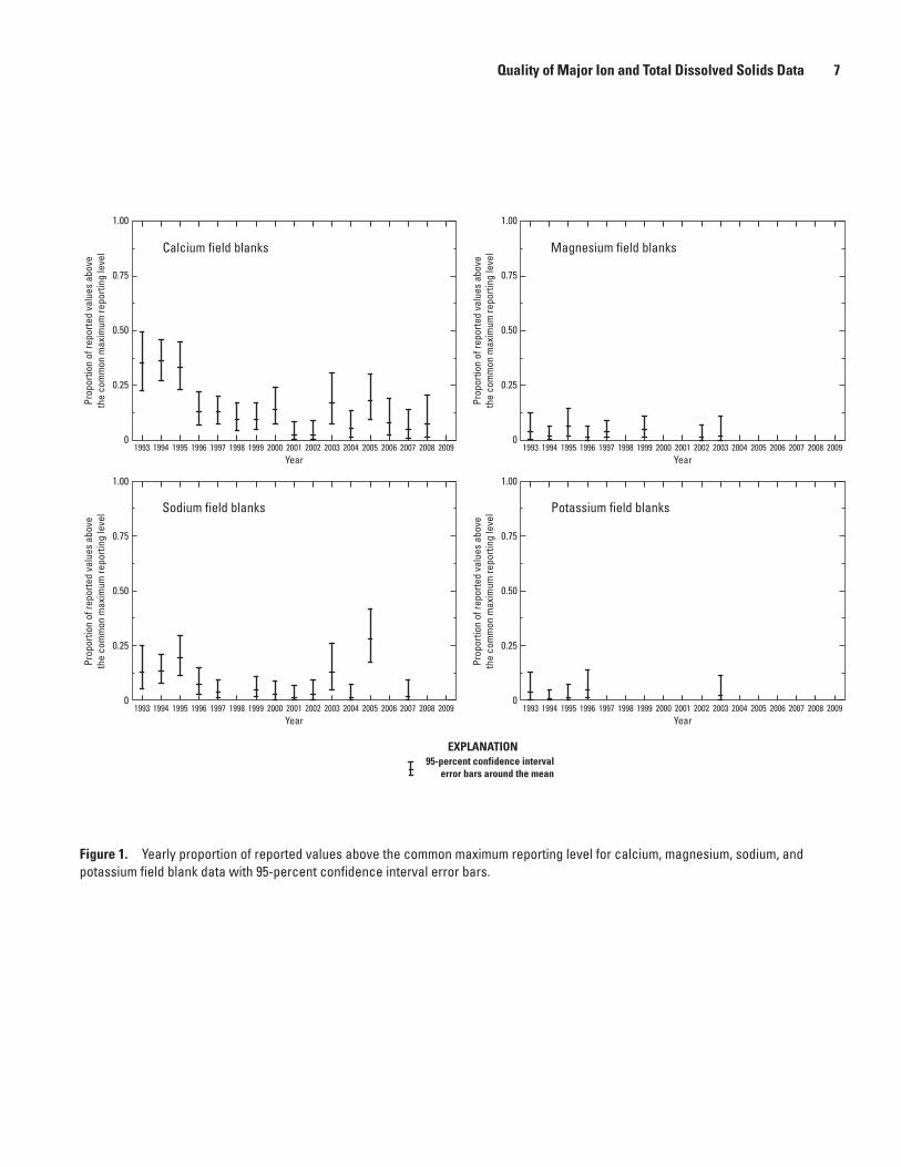
Figures 1. Graphs showing yearly proportion of reported values above the common maximum

reporting level for calcium, magnesium, sodium, and potassium field blank data with 95-percent confidence interval error bars ......................................................................7

2. Graphs showing yearly proportion of reported values above the common maximum reporting level for chloride, sulfate, fluoride, and silica field blank data with 95-percent confidence interval error bars ......................................................................8

3. Graph showing yearly proportion of reported values above the common maximum reporting level for total dissolved solids field blank data with 95-percent confidence interval error bars .........................................................................................................................9

4. Graph showing upper 99-percent confidence limit for percentiles of chloride contamination in all groundwater samples based on data from field blanks .....................9

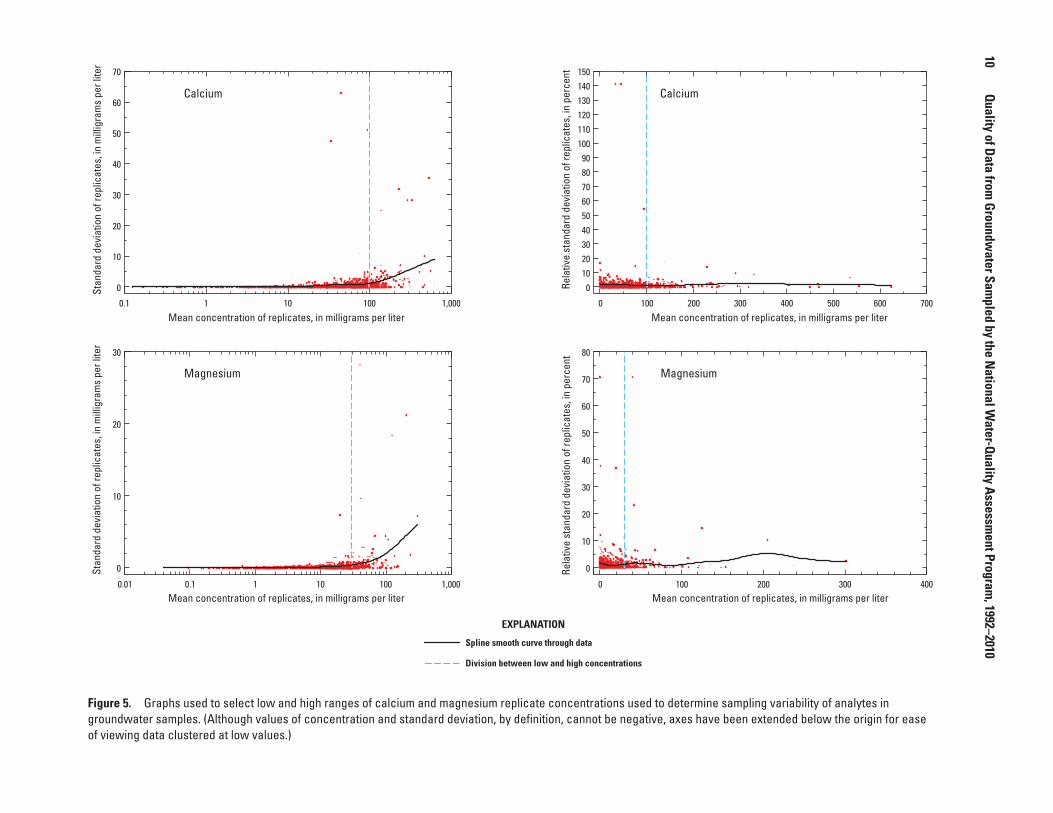
5. Graphs used to select low and high ranges of calcium and magnesium replicate concentrations used to determine sampling variability of analytes in groundwater samples ............................................................................................................10

6. Graphs used to select low and high ranges of sodium and potassium replicate concentrations used to determine sampling variability of analytes in groundwater samples ............................................................................................................11

7. Graphs used to select low and high ranges of chloride and sulfate replicate concentrations used to determine sampling variability of analytes in groundwater samples ............................................................................................................12

8. Graphs used to select low and high ranges of fluoride and silica replicate concentrations used to determine sampling variability of analytes in groundwater samples ............................................................................................................13

9. Graphs used to select low and high ranges of total dissolved solids replicate concentrations used to determine sampling variability of analytes in groundwater samples ............................................................................................................14

10. Time-series plot showing a linear trend in the standard deviation of chloride replicates that had a mean concentration less than 100 milligrams per liter ..................17

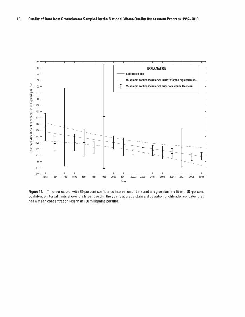
11. Time-series plot with 95-percent confidence interval error bars and a regression line fit with 95-percent confidence interval limits showing a linear trend in the yearly average standard deviation of chloride replicates that had a mean concentration less than 100 milligrams per liter ...................................................................18

12. Graphs used to select low and high ranges of calcium replicate concentrations used to determine sampling variability of calcium in groundwater samples collected from 1997 through 2009 ............................................................................................19

vi

Tables 1. Number of quality-control groundwater samples collected in each of the 48 National

Water-Quality Assessment Program study units that were used for the data analysis in this report ...................................................................................................................................3

2. Upper 99-percent confidence limits for contamination by analytes in specified percentiles of all groundwater samples based on data from field blanks prepared at groundwater sample collection sites and maximum affected concentrations calculated based on the 99-percent upper confidence limit for the 95th percentile ........4

3. Replicate set reporting levels and number of nondetects for each analyte ......................4 4. Estimates of sampling variability for analytes in groundwater samples collected

from 1992 to 2009 .........................................................................................................................16 5. Estimates of sampling variability for analytes in groundwater samples collected

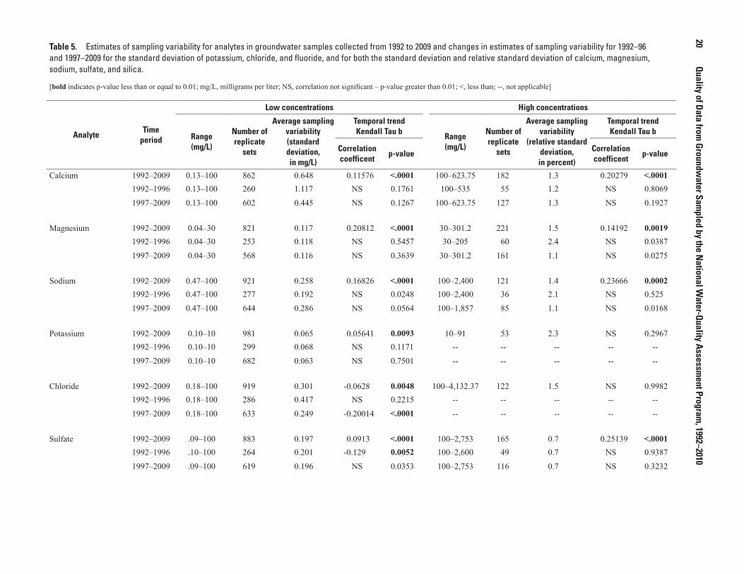
from 1992 to 2009 and changes in estimates of sampling variability for 1992–96 and 1997–2009 for the standard deviation of potassium, chloride, and fluoride, and for both the standard deviation and relative standard deviation of calcium, magnesium, sodium, sulfate, and silica ..................................................................................20

6. Changes in sampling variability for calcium in groundwater samples collected from 1992 to 2009 .........................................................................................................................21

7. Most appropriate sampling variabilities for application to environmental data on the basis of low and high concentrations and year ........................................................22

Abbreviations, Acronyms, and Conversion Factorsmg/L milligrams per liter

NAWQA National Water-Quality Assessment

QC quality control

RSD relative standard deviation

SMCL Secondary Maximum Contaminant Level

UCL upper confidence limit

USEPA U.S. Environmental Protection Agency

USGS U.S. Geological Survey

Temperature in degrees Celsius (°C) may be converted to degrees Fahrenheit (°F) as follows:

°F=(1.8×°C)+32

Temperature in degrees Fahrenheit (°F) may be converted to degrees Celsius (°C) as follows:

°C=(°F-32)/1.8

Concentrations of chemical constituents in water are given in milligrams per liter (mg/L), which is approximately equal to parts per million.


By Eliza L. Gross, Bruce D. Lindsey, and Michael G. Rupert

AbstractProper interpretation of water quality requires consid-

eration of the effects that contamination bias and sampling variability might have on measured analyte concentrations. The effect of contamination bias and sampling variability on major ion and total dissolved solids data in water samples collected in 48 of the 52 National Water-Quality Assessment Program study units from 1992 to 2010 is discussed in this report. Contamination bias and sampling variability can occur as a result of sample collection, processing, shipping, and analysis. Contamination bias can adversely affect interpreta-tion of measured concentrations in comparison to standards or criteria. Sampling variability can help determine the reproducibility of an individual measurement or whether two measurements are different.

Field blank samples help determine the frequency and magnitude of contamination bias, and replicate samples help determine the sampling variability (error) of measured analyte concentrations. Quality control data were evaluated for calcium, magnesium, sodium, potassium, chloride, sulfate, fluoride, silica, and total dissolved solids. A 99-percent upper confidence limit is calculated from field blanks to assess the potential for contamination bias. For magnesium, potassium, chloride, sulfate, and fluoride, potential contamination in more than 95 percent of environmental samples is less than or equal to the common maximum reporting level. Contamina-tion bias has little effect on measured concentrations greater than 4.74 mg/L (milligrams per liter) for calcium, 14.98 mg/L for silica, 4.9 mg/L for sodium, and 120 mg/L for total dis-solved solids. Estimates of sampling variability are calculated for high and low ranges of concentration for major ions and total dissolved solids. Examples showing the calculation of confidence intervals and how to determine whether mea-sured differences between two water samples are significant are presented.

IntroductionThe U.S. Geological Survey’s (USGS) National-Water

Quality Assessment (NAWQA) Program was implemented in 1991 in order to describe current water-quality conditions and how they are changing and to improve scientific and public understanding of natural and human factors impacting those conditions. These objectives are being achieved through exten-sive monitoring within 52 study units, which consist of large river basin and aquifer systems throughout the United States. In Cycle I (1991–2001) and Cycle II (2002–12), much of the work involved gathering comparable information on water quality in both surface water and groundwater.

Estimates of contamination bias and sampling variability resulting from sample collection, processing, shipment, and laboratory analysis are needed to quantify how much variabil-ity in water-quality measurements can be explained by field and laboratory methods, as compared to environmental factors (Mueller and Titus, 2005). Quality-control (QC) samples, such as field blank or replicate samples, are collected at the same time as the environmental samples in order to evaluate contamination bias and sampling variability. Contamination bias is the systematic error that can occur during sample col-lection, processing, shipping, or laboratory analysis. Contami-nants can be introduced into water samples by exposure to airborne gases and particulates or from inadequately cleaned sample collection or analytical equipment (Mueller and Titus, 2005). Variability is the degree of random error in independent measurements of the same quantity, and “sampling variability” (termed by Mueller, 1998, p. vii) is the variability introduced by sample collection, field processing, shipping, and labora-tory analysis. Contamination bias and sampling variability are evaluated by collecting and analyzing QC samples. The frequency and magnitude of contamination bias are deter-mined from field blank samples, and the sampling variabil-ity of measured analyte concentrations is determined from

2 Quality of Data from Groundwater Sampled by the National Water-Quality Assessment Program, 1992–2010

replicate samples. The distribution of concentrations in field blank samples is used to estimate the potential distribution of contamination in the environmental samples. Similarly, the distribution of variability in the replicate sets is used to estimate potential sampling variability in the results from environmental samples. Estimates from a particular set of field blanks or replicates can be applied to a particular set of environmental samples to describe similar sample collection and analytical methods, sample collection site characteris-tics, and sample collection during a specific time period.

Purpose and Scope

This report describes the quality of major ion and total dissolved solids data in groundwater samples collected in 48 of the 52 NAWQA study units from 1992 to 2010. The QC analysis is used to (1) describe the frequency and magnitude of contamination using field blank samples; (2) evaluate sampling variability of the groundwater-quality data using replicate samples; and (3) identify potential effects of bias and sampling variability in interpreting the major ion and total dissolved solids data. Major ions reviewed in this report include calcium, magnesium, sodium, potassium, chlo-ride, sulfate, fluoride, and silica. Although bicarbonate and carbonate are also major ions, these were not included in the study since they are computed from field measurement of alkalinity rather than laboratory measurements.

Environmental and Quality-Control Data

This report evaluates major ion and total dissolved solids data from groundwater and QC samples collected during 1992–2010 at locations within 48 of the 52 NAWQA study units. Contamination bias and sampling variability were assumed to be the same or similar in all 48 NAWQA study units even though this may not necessarily always be the case. The number of field blank and replicate samples used in this report from each study unit are listed in table 1. Groundwater samples were collected using the protocols for the collection of QC samples for NAWQA study-unit investigations documented by Koterba and others (1996) and were analyzed at the USGS National Water Quality Laboratory (NWQL) in Denver, Colorado (Shelton, 1994; U.S. Geological Survey, variously dated). Chemical analysis results on QC samples and associated environmental samples were compiled from the USGS’s NAWQA Data Warehouse (http://water.usgs.gov/nawqa/data). Data used in this report were retrieved from the NAWQA Data Warehouse during March 2010 and reviewed for consistency to identify and correct errors.

Types of Quality-Control Samples

A blank is a QC water sample that is intended to be free of and not interfere with the determination of the analytes of interest (Mueller and Titus, 2005). Blank samples are used to test for bias that could result from contamination during any stage of the sample collection and analysis process. A field blank is a specific type of blank sample used to demonstrate that (1) equipment has been adequately cleaned to remove contamination introduced from water samples obtained at previous sites; (2) sample collection and processing have not resulted in contamination; and (3) sample handling, shipping, and laboratory analysis have not introduced contamination (Mueller and Titus, 2005). Field blank samples are the only type of QC blank samples evaluated in this study.

Replicates are two or more QC samples that are collected or processed in such a manner that the replicate samples are thought to be essentially identical in composition (Mueller and Titus, 2005). Replicate samples are used to measure the sampling variability introduced during sample processing and analysis. Sequential replicates (multiple replicate samples collected at the same location one right after the other) were collected for this study. In addition to sampling variability, sequential replicates can include a small amount of envi-ronmental variability, though this is generally negligible for groundwater samples since wells are pumped until conditions are stable prior to sample collection.

Compilation of Data

Field blank data with multiple reporting levels were aggregated for each analyte in relation to the highest or most frequently used reporting level, which is referred to in this report as a “common maximum reporting level” (Apodaca and others, 2006). For each analyte (except for total dissolved solids) the highest reporting level in the field blank samples was used as a common maximum reporting level because these levels were consistent with detection limits observed in 1993–2010 blind spike samples collected through the USGS Branch of Quality System’s Inorganic Blind Spike Sample Project. The most frequently used reporting level was used as the common maximum reporting level for total dissolved solids because only one groundwater sample represented the highest reporting level, and the highest reporting level was not consistent with any of the total dissolved solids detection limits observed in 1993–2010 blind spike samples collected through the Inorganic Blind Spike Sample Project. Com-mon maximum reporting levels for each analyte are listed in table 2. A single common reporting level can lead to loss of information because some quantified results will be censored, especially for analytes with multiple reporting levels that are less than the defined common maximum reporting level. Since only slight differences occurred among reporting levels

Environmental and Quality-Control Data 3

Table 1. Number of quality-control groundwater samples collected in each of the 48 National Water-Quality Assessment Program study units that were used for the data analysis in this report.

Study-unit abbreviation

Study-unit nameNumber of

field blanksNumber of

replicate setsACAD Acadian-Pontchartrain Drainages 15 32ACFB Apalachicola-Chattahoochee-Flint River Basin 19 43ALBE Albemarle-Pamlico Drainage Basin 30 21ALMN Allegheny and Monongahela River Basins 13 13CAZB Central Arizona Basins 42 26CCYK Central Columbia Plateau - Yakima River Basin 28 22CNBR Central Nebraska Basins 30 20CONN Connecticut, Housatonic, and Thames River Basins 35 19COOK Cook Inlet Basin 7 2DELR Delaware River Basin 16 6EIWA Eastern Iowa Basins 33 41GAFL Georgia-Florida Coastal Plain 18 30GRSL Great Salt Lake Basins 43 23HDSN Hudson River Basin 16 9HPGW High Plains Regional Groundwater Study 59 55KANA Kanawha - New River Basins 16 1LERI Lake Erie - Lake Saint Clair Drainages 15 16LINJ Long Island - New Jersey Coastal Drainages 47 34LIRB Lower Illinois River Basin 40 17LSUS Lower Susquehanna River Basin 0 17MISE Mississippi Embayment 26 23MOBL Mobile River Basin 15 12NECB New England Coastal Basins 39 14NROK Northern Rockies Intermontane Basins 23 14NVBR Las Vegas Valley Area and the Carson and Truckee River Basins 32 17OAHU Oahu 8 4OZRK Ozark Plateaus 18 16PODL Potomac River Basin and Delmarva Peninsula 38 64PUGT Puget Sound Basin 17 13REDN Red River of the North Basin 26 30RIOG Rio Grande Valley 31 28SACR Sacramento River Basin 29 20SANA Santa Ana Basin 18 19SANJ San Joaquin-Tulare Basins 46 55SANT Santee River Basin and Coastal Drainages 41 25SCTX South-Central Texas 49 32SOFL Southern Florida 28 14SPLT South Platte River Basin 44 43TENN Tennessee River Basin 22 17TRIN Trinity River Basin 16 19UCOL Upper Colorado River Basin 25 15UIRB Upper Illinois River Basin 22 13UMIS Upper Mississippi River Basin 16 27USNK Upper Snake River Basin 32 27WHMI White, Great, and Little Miami River Basins 37 36WILL Willamette Basin 22 2WMIC Western Lake Michigan Drainages 5 20YELL Yellowstone River Basin 12 11

Total 1,259 1,077


for each analyte, censoring field blank data to the appropriate common maximum reporting level removed minor inconsis-tencies caused by multiple reporting levels.

Replicate data were not censored to a common maximum reporting level because sampling variability of replicates can only be analyzed when both samples in a replicate pair have detections. Reporting levels and the number of nondetections in replicate sets for all analytes are listed in table 3. Replicate

sets consisting of all nondetections were excluded from the analysis of sampling variability (Martin, 2002). In addition, replicate pairs with detections in one sample but not in both were excluded from analysis due to inconsistency in detec-tions. Less than 4 percent of the replicate pairs for fluoride represent pairs with uncertain detections, and less than 1 per-cent of replicate pairs represent pairs with uncertain detections for all other analytes.

Table 2. Upper 99-percent confidence limits for contamination by analytes in specified percentiles of all groundwater samples based on data from field blanks prepared at groundwater sample collection sites and maximum affected concentrations calculated based on the 99-percent upper confidence limit for the 95th percentile.

[mg/L, milligrams per liter]

AnalyteNumber of field blanks

Common maximum reporting

level (mg/L)

Field blanks with reported values greater

than the common maximum reporting level

Upper 99-percent confidence limit (mg/L)

Maximum affected

concentration (mg/L)

Number Percent75th

percentile90th

percentile95th

percentile99th

percentile

Calcium 1,253 0.10 181 14.4 0.1 0.18 0.47 3.5 4.74Magnesium 1,253 .10 23 1.8 0.1 0.1 0.1 1.7 1.00Sodium 1,253 .20 84 6.7 0.2 0.2 0.5 4.4 4.90Potassium 1,104 .24 9 0.8 0.24 0.24 0.24 2.30 2.40Chloride 1,100 .30 17 1.5 0.3 0.3 0.3 1.7 3.00Sulfate 1,099 .31 10 0.9 0.31 0.31 0.31 1.89 3.10Fluoride 1,100 .20 4 0.4 0.2 0.2 0.2 0.2 2.00Silica 1,253 .20 121 9.7 0.2 0.29 1.50 10 14.98Total dissolved solids 1,083 10 52 4.8 10 10 12 33 120.00

Table 3. Replicate set reporting levels and number of nondetects for each analyte.

[bold indicates most common reporting level for each analyte; mg/L, milligrams per liter]

AnalyteTotal number of replicate

setsReporting levels

Number of replicate sets with nondetects

for both groundwater samples

Number of replicate sets with nondetects

for one groundwater sample

Number of replicate sets used for study

Calcium 1,045 0.02 0 1 1,044Magnesium 1,045 0.01 0 3 1,042Sodium 1,045 0.2 0 3 1,042Potassium 1,045 0.1, 0.06 6 5 1,034Chloride 1,044 1.0, 0.1 0 3 1,041Sulfate 1,074 0.31, 0.18, 0.1, 0.01 20 6 1,048Fluoride 1,043 0.5, 0.2, 0.171, 0.17, 0.16, 0.131, 0.123,

0.12, 0.115, 0.104, 0.101, 0.1, 0.096, 0.091, 0.08, 0.078, 0.06, 0.058, 0.055, 0.053, 0.051, 0.019, 0.007

289 36 718

Silica 1,042 0.1, 0.01 0 2 1,040Total dissolved solids 1,008 10 1 0 1,007

Methods of Data Analysis 5

Methods of Data AnalysisContamination bias and sampling variability can be eval-

uated through statistical analysis of field blank and replicate samples, respectively. The primary purpose of evaluating con-tamination bias and sampling variability is to determine their effects on interpretation of the associated environmental data.

Methods Used to Determine Contamination Bias

The purpose of analyzing field blanks is to estimate the amount of contamination that might have been introduced during the collection, processing, shipping, and analyzing of environmental samples. The frequency and distribution of contamination identified in field blank samples is assumed to apply to environmental samples because both samples were collected, processed, shipped, and analyzed in the same way, at the same or similar sites, and during the same time period. Ideally, the bias introduced by contamination will be so small that concentrations in field blanks are less than the laboratory detection limit (Mueller and Titus, 2005).

Field blank data collected during the sample collection period were analyzed for temporal trends to determine if con-tamination bias changed over time. The proportion of reported values above the common maximum reporting level was calculated for each year from 1993 to 2009 for each analyte. The upper and lower 95-percent confidence intervals for each yearly proportion were calculated and plotted as error bars sur-rounding the proportion, and the plotted data were analyzed to evaluate trends over time.

To assess the potential for contamination at or above the common maximum reporting level for each analyte, upper confidence limits (UCLs) were constructed for percentiles of the distribution of concentration in the field blanks. The UCL is the maximum contamination expected in a speci-fied percentage of water samples. Therefore, the 99-percent UCL for the 95th percentile indicates that with 99-percent confidence, the resulting amount of contamination would be exceeded in no more than 5 percent of water samples. The 99-percent UCL at the 95th percentile also can be explained as the maximum contamination expected in 95 percent of the samples with only a 1-percent chance that the contamination has been underestimated.

Statistical techniques that assume normality when calculating the UCL are not applicable since the distribution of concentrations in field blanks can be highly skewed. A method described by Hahn and Meeker (1991) is appropriate for skewed data and can be used to determine a distribution-free UCL for a percentile. The UCL is calculated using order statistics, which rank data values from small to large, and a binomial probability (Mueller and Titus, 2005). Mueller and Titus include an example of this calculation (Mueller and

Titus, 2005, p. 4 and 6). A one-sided 99-percent UCL was calculated at the 75th, 90th, 95th, and 99th percentiles for analyte concentrations in field blanks using the SAS statistical software (SAS Institute Inc., 1990).

Methods Used to Determine Sampling Variability

Sampling variability can be estimated by using some measure of the dispersion of repeated measurements, such as the standard deviation of field replicates (Mueller and Titus, 2005). Because sampling variability of replicates can only be determined when both samples in a pair have detections, only replicate pairs with detections were included (Apodaca and others, 2006). Sampling variability of replicate data was ana-lyzed according to different statistical measures over different concentration ranges. Over a low range of concentrations, standard deviation of replicates generally is uniform, but at higher concentrations, standard deviation tends to increase in proportion to concentration (Mueller and Titus, 2005). Within this high range, the relative standard deviation (RSD), defined as the standard deviation divided by the mean concentration, is generally uniform. The RSD is also known as the coefficient of variation (Mueller and Titus, 2005).

Sampling variability over the range of observed concen-trations can be approximated by dividing the replicate data into segments where either the standard deviation or the RSD is relatively constant (Anderson, 1987). Over the low-concen-tration range, sampling variability is estimated as the average standard deviation of replicates; over the high-concentration range, sampling variability is estimated as the average RSD (Mueller and Titus, 2005). Selection of high and low concen-tration ranges can be performed using graphical analysis of standard deviation and RSD in relation to mean concentration for each replicate set. Approximate boundary values between ranges can be determined by the change in slope of a curve, such as a spline smooth (SAS Institute Inc., 1990) or loess (local regression) curve (S-Plus, 2002) through the center of the data. Adjustments could be necessary if the average low-range standard deviation and high-range RSD do not intersect at the boundary.

Standard deviation and RSD of replicates were analyzed for temporal trends using Kendall’s tau-b, which is a non-parametric measure of association based on concordances and discordances in paired observations (SAS Institute Inc., 1990). Where temporal trends were statistically significant (p < 0.1), changes in laboratory methods, reported concentrations, or sample collection techniques were examined and data were further analyzed to calculate appropriate sampling variabilities for each analyte.

After calculating sampling variability for low- and high-concentration ranges of replicate data, confidence intervals


can be determined for any one measurement. The confidence interval for a concentration measured in a single water sample is defined as:

[CL ,CU] = C ± Z(1 – α/2) σ , (1)

where CL,CU are the lower and upper limits of

concentration for the 100(1 – α)-percent confidence interval,

C is the individual measured concentration, Z is the ordinate if the normal curve (Z-value)

contains 100(1 – α) percent of the distribution,

α is the probability that the confidence interval does not include the true concentration, and

σ is the sampling variability for the measured concentration.

If the measured concentration is in the low range, σ is the average standard deviation of replicates within that range. If the measured concentration is in the high range, σ = C (RSD/100).

The error inherent in a single measurement of con-centration due to sampling variability is represented in equation 1 by the term Z(1 – α/2) σ. It is not possible, with 100(1 – α)-percent confidence, to determine whether the con-centration in the water sample exceeds the standard if a single measurement differs from a standard by less than this error.

For a mean concentration (C) from multiple water sam-ples, the confidence interval for the true mean is calculated:

[ , ] ( / )C C C ZnL U a= ± −1 2σ

, (2)

where n is the number of water samples, C is the mean concentration for these water

samples, and the other variables are as previously defined in equation 1.

Again, the second term of equation 2 represents the error due to sampling variability, but in this instance it includes the number of water samples as well as the standard devia-tion. Thus, the error inherent in a mean concentration due to sampling variability can be decreased by collecting more water samples. This error can be considered the minimum that is typically achievable for determining a mean concentration in the absence of environmental variability. A determination of statistical significance is unlikely for a difference between two mean concentrations that is less than the sum of their inher-ent errors; therefore, small but true environmental differences might not be detected (Mueller and Titus, 2005, p. 7).

Quality of Major Ion and Total Dissolved Solids Data

Groundwater samples were analyzed for the following analytes:

• calcium

• magnesium

• sodium

• potassium

• chloride

• sulfate

• fluoride

• silica

• total dissolved solids dried at 180°C

The QC samples collected to analyze the quality of the NAWQA data included field blanks prepared using inorganic grade laboratory blank waters that were pumped through the groundwater sample collection equipment using pumps designed to prevent contamination. Groundwater replicates were collected sequentially as water was pumped from the well.

Contamination Bias

The relation between analyte concentrations and the dates on which field blanks were collected was analyzed to identify possible temporal trends in contamination. Plots were created showing the proportion of reported values above the common maximum reporting level and their 95-percent confidence intervals for years 1993–2009 (figs. 1–3). Since only a few groundwater samples were available for 1992 and 2010, data from these years were omitted. Year-by-year plots of magne-sium, potassium, chloride, sulfate, fluoride, and total dissolved solids show that proportions of reported values above the common maximum threshold and a majority of their upper confidence levels were consistently below 0.25 from 1993 to 2009. Calcium, silica, and sodium had higher proportions from 1993–95 than for the remaining years, which also cor-responds with the time period when sample collection began. Sodium and silica also had proportions above 0.50 for 2005, but the proportions for 1996–2004 and 2006–09 remained fairly consistent. Overall, proportions of reported values above the common maximum reporting level and their 95-percent confidence intervals were (1) consistent for all of the years or (2) higher from 1993 to 1995, when the sample collection

Quality of Major Ion and Total Dissolved Solids Data 7

Figure 1. Yearly proportion of reported values above the common maximum reporting level for calcium, magnesium, sodium, and potassium field blank data with 95-percent confidence interval error bars.

Potassium field blanksSodium field blanks

Magnesium field blanks

Prop

ortio

n of

repo

rted

valu

es a

bove

the

com

mon

max

imum

repo

rting

leve

l

0

0.25

0.50

0.75

1.00

Year1993 1994 1995 1996 1997 1998 1999 2000 2001 2002 2003 2004 2005 2006 2007 2008 2009

Prop

ortio

n of

repo

rted

valu

es a

bove

the

com

mon

max

imum

repo

rting

leve

l

0

0.25

0.50

0.75

1.00

Year1993 1994 1995 1996 1997 1998 1999 2000 2001 2002 2003 2004 2005 2006 2007 2008 2009

Prop

ortio

n of

repo

rted

valu

es a

bove

the

com

mon

max

imum

repo

rting

leve

l

0

0.25

0.50

0.75

1.00

Year1993 1994 1995 1996 1997 1998 1999 2000 2001 2002 2003 2004 2005 2006 2007 2008 2009

Prop

ortio

n of

repo

rted

valu

es a

bove

the

com

mon

max

imum

repo

rting

leve

l

0

0.25

0.50

0.75

1.00

Year1993 1994 1995 1996 1997 1998 1999 2000 2001 2002 2003 2004 2005 2006 2007 2008 2009

Calcium field blanks

95-percent confidence interval error bars around the mean

EXPLANATION


Figure 2. Yearly proportion of reported values above the common maximum reporting level for chloride, sulfate, fluoride, and silica field blank data with 95-percent confidence interval error bars.

Silica field blanksFluoride field blanks

Sulfate field blanks

Prop

ortio

n of

repo

rted

valu

es a

bove

the

com

mon

max

imum

repo

rting

leve

l

0

0.25

0.50

0.75

1.00

Year1993 1994 1995 1996 1997 1998 1999 2000 2001 2002 2003 2004 2005 2006 2007 2008 2009

Prop

ortio

n of

repo

rted

valu

es a

bove

the

com

mon

max

imum

repo

rting

leve

l

0

0.25

0.50

0.75

1.00

Year1993 1994 1995 1996 1997 1998 1999 2000 2001 2002 2003 2004 2005 2006 2007 2008 2009

Prop

ortio

n of

repo

rted

valu

es a

bove

the

com

mon

max

imum

repo

rting

leve

l

0

0.25

0.50

0.75

1.00

Year1993 1994 1995 1996 1997 1998 1999 2000 2001 2002 2003 2004 2005 2006 2007 2008 2009

Prop

ortio

n of

repo

rted

valu

es a

bove

the

com

mon

max

imum

repo

rting

leve

l

0

0.25

0.50

0.75

1.00

Year1993 1994 1995 1996 1997 1998 1999 2000 2001 2002 2003 2004 2005 2006 2007 2008 2009

Chloride field blanks


EXPLANATION


program began, and were consistent for the remaining years, except for the high proportion for 2005 for silica and sodium. The distribution of proportions of reported values above the common maximum reporting level for each analyte did not appear to be due to an overall increase or decrease during the period of record, but could have been affected by changes in sample collection frequency and reporting level.

Data from all field blanks were used to calculate UCLs for selected percentiles of contamination, which were then assumed to be applicable to all environmental samples col-lected from 1992 to 2010. The 99-percent UCL was selected, and calculations were made for the 75th, 90th, 95th, and 99th percentiles (table 2). The potential contamination in ground-water is estimated to be no greater than the common maxi-mum reporting level for all analytes in at least 75 percent of all samples. In at least 90 percent of all groundwater samples, potential contamination is estimated to be no greater than the common maximum reporting level for all analytes except calcium and silica in groundwater. Plots of the 99-percent UCLs show that potential contamination remains relatively low through at least the 95th percentiles for all analytes. For example, figure 4 shows potential contamination for chloride is not likely to exceed the common maximum reporting level of 0.30 mg/L in 97 percent of all groundwater samples.

Sampling Variability

Sampling variability within replicate samples collected at groundwater sites was estimated using the standard deviation over a low range of concentrations and the relative standard deviation (RSD) over a high range of concentrations. For each

analyte, replicate standard deviation and RSD were graphed with the mean concentrations for each set of replicates in order to determine the division between low-range and high-range concentrations (figs. 5–9). Concentrations are shown on a logarithmic scale in the standard deviation graphs so that the lower range is emphasized. Each graph includes a smooth curve through the data points showing the general relation between concentrations and standard deviation or RSD. Where the smooth curve is roughly horizontal, there is no relation between concentrations and standard deviation or RSD. Over this range of concentration, sampling variability is considered constant. Divisions between low-range and high-range con-centrations were defined by finding a point on the x-axis below which the curve for standard deviation or RSD was essentially horizontal and above which the curve for RSD was essentially horizontal. These boundary concentrations are represented on each graph with a vertical dashed line. Sampling variability for each analyte was estimated as the average standard deviation for the low range of concentrations or the average RSD for the high range of concentrations after low-range and high-range concentrations for each analyte were defined.

Trends in Sampling VariabilityTemporal trends in the standard deviation and RSD were

analyzed for each analyte in order to examine the stability of each sampling variability value over the period of record. Groundwater samples in the low range of mean concentration

Figure 3. Yearly proportion of reported values above the common maximum reporting level for total dissolved solids field blank data with 95-percent confidence interval error bars.

Prop

ortio

n of

repo

rted

valu

es a

bove

the

com

mon

max

imum

repo

rting

leve

l

0

0.25

0.50

0.75

1.00

Year1993 1994 1995 1996 1997 1998 1999 2000 2001 2002 2003 2004 2005 2006 2007 2008 2009

Total dissolved solids field blanks


EXPLANATION

Chlo

ride

conc

entra

tion,

in m

illig

ram

s pe

r lite

r

0.3

0.2

0.4

0.5

0.6

0.7

0.8

0.9

1.0

1.1

1.2

1.3

1.4

1.5

1.6

1.7

Percentile40 50 60 70 80 90 100

Groundwater chloride concentrations by percentile

Common maximum reporting level

EXPLANATION

Figure 4. Upper 99-percent confidence limit for percentiles of chloride contamination in all groundwater samples based on data from field blanks.

10

Quality of Data from Groundw

ater Sampled by the N

ational Water-Quality Assessm

ent Program, 1992–2010

Figure 5. Graphs used to select low and high ranges of calcium and magnesium replicate concentrations used to determine sampling variability of analytes in groundwater samples. (Although values of concentration and standard deviation, by definition, cannot be negative, axes have been extended below the origin for ease of viewing data clustered at low values.)

Stan

dard

dev

iatio

n of

repl

icat

es, i

n m

illig

ram

s pe

r lite

r

0

10

20

30

40

50

60

70

Stan

dard

dev

iatio

n of

repl

icat

es, i

n m

illig

ram

s pe

r lite

r

0

10

20

30

Mean concentration of replicates, in milligrams per liter0.1 1 10 100 1,000

Calcium

Mean concentration of replicates, in milligrams per liter0 100 200 300 400 500 600 700

Mean concentration of replicates, in milligrams per liter0.01 0.1 1 10 100 1,000

Mean concentration of replicates, in milligrams per liter0 100 200 300 400

Rela

tive

stan

dard

dev

iatio

n of

repl

icat

es, i

n pe

rcen

t

0102030405060708090

100110120130140150

Calcium

Magnesium

Rela

tive

stan

dard

dev

iatio

n of

repl

icat

es, i

n pe

rcen

t0

10

20

30

40

50

60

70

80

Magnesium

EXPLANATION

Spline smooth curve through data

Division between low and high concentrations


11

Figure 6. Graphs used to select low and high ranges of sodium and potassium replicate concentrations used to determine sampling variability of analytes in groundwater samples. (Although values of concentration and standard deviation, by definition, cannot be negative, axes have been extended below the origin for ease of viewing data clustered at low values.)

Stan

dard

dev

iatio

n of

repl

icat

es, i

n m

illig

ram

s pe

r lite

r

0

10

20

30

40

50

60

70

80

90

100St

anda

rd d

evia

tion

of re

plic

ates

, in

mill

igra

ms

per l

iter

0

8

10

4

6

2

12

Mean concentration of replicates, in milligrams per liter0.1 1 10 100 1,000 10,000

Sodium

Mean concentration of replicates, in milligrams per liter0 1,000 2,000 3,000

Mean concentration of replicates, in milligrams per liter0.01 0.1 1 10 100


Rela

tive

stan

dard

dev

iatio

n of

repl

icat

es, i

n pe

rcen

t

0

10

20

30

40

50

Sodium

Potassium

Rela

tive

stan

dard

dev

iatio

n of

repl

icat

es, i

n pe

rcen

t

0

10

20

30

40

50

60

80

70

90

100

Potassium

EXPLANATION



12





Figure 7. Graphs used to select low and high ranges of chloride and sulfate replicate concentrations used to determine sampling variability of analytes in groundwater samples. (Although values of concentration and standard deviation, by definition, cannot be negative, axes have been extended below the origin for ease of viewing data clustered at low values.)

Stan

dard

dev

iatio

n of

repl

icat

es, i

n m

illig

ram

s pe

r lite

r

0

10

20

30

40

50

60

70

90

80

110

100

120

130

Stan

dard

dev

iatio

n of

repl

icat

es, i

n m

illig

ram

s pe

r lite

r

0

120

150

60

90

30

110

140

170160

50

80

20

100

130

40

70

10

180

Mean concentration of replicates, in milligrams per liter0.1 1 10 100 1,000 10,000

Chloride

Mean concentration of replicates, in milligrams per liter0 1,000 2,000 3,000 4,000 5,000

Mean concentration of replicates, in milligrams per liter0.01 0.1 1 10 10,000100 1,000

Mean concentration of replicates, in milligrams per liter0 1,000 2,000 3,000

Rela

tive

stan

dard

dev

iatio

n of

repl

icat

es, i

n pe

rcen

t

0

10

20

30

40

50

Chloride

Sulfate

Rela

tive

stan

dard

dev

iatio

n of

repl

icat

es, i

n pe

rcen

t0

10

20

30

40

50

60

70

Sulfate

EXPLANATION




13

Figure 8. Graphs used to select low and high ranges of fluoride and silica replicate concentrations used to determine sampling variability of analytes in groundwater samples. (Although values of concentration and standard deviation, by definition, cannot be negative, axes have been extended below the origin for ease of viewing data clustered at low values.)

Stan

dard

dev

iatio

n of

repl

icat

es, i

n m

illig

ram

s pe

r lite

r

00.10.20.30.40.50.60.7

0.90.8

1.2

1.0

1.4

1.1

1.3

1.5St

anda

rd d

evia

tion

of re

plic

ates

, in

mill

igra

ms

per l

iter

0

10

20

30

Mean concentration of replicates, in milligrams per liter0.01 0.1 1 10

Fluoride

Mean concentration of replicates, in milligrams per liter0 1 2 43 65 7 8

Mean concentration of replicates, in milligrams per liter1 10 100


Rela

tive

stan

dard

dev

iatio

n of

repl

icat

es, i

n pe

rcen

t

0

20

40

60

80

90

100

110

120

10

30

50

70

130

Fluoride

Silica

Rela

tive

stan

dard

dev

iatio

n of

repl

icat

es, i

n pe

rcen

t0

20

40

60

80

100

120

150

10

30

50

70

90

110

130140 Silica

EXPLANATION




Figure 9. Graphs used to select low and high ranges of total dissolved solids replicate concentrations used to determine sampling variability of analytes in groundwater samples. (Although values of concentration and standard deviation, by definition, cannot be negative, axes have been extended below the origin for ease of viewing data clustered at low values.)

Stan

dard

dev

iatio

n of

repl

icat

es, i

n m

illig

ram

s pe

r lite

r

0

10

20

30

Mean concentration of replicates, in milligrams per liter1 10 100


Rela

tive

stan

dard

dev

iatio

n of

repl

icat

es, i

n pe

rcen

t

0

20

40

60

80

100

120

150

10

30

50

70

90

110

130140

EXPLANATION



Total dissolved solids

Total dissolved solids


were analyzed for trends in standard deviation, whereas groundwater samples in the high range of mean concentration were analyzed for trends in RSD. Trends were identified as statistically significant (p < 0.01) for 13 of the 18 measures of sampling variability listed in table 4 using the Mann-Kendall trend test. Statistically significant trends were identified for the standard deviation of potassium, chloride, and fluoride, and for both the standard deviation and RSD of calcium, magnesium, sodium, sulfate, and silica.

For each of the analytes, the number of significant decimal places in the reported concentrations was increased in the beginning of 1997. Before the change in 1997, the magnitude of differences between pairs of replicate concen-trations was limited to a small number of values, leading to linear patterns in standard deviations and RSDs before 1997, as shown in figure 10, for example: the difference between two rounded concentrations could be 0.0 or 0.1, but not 0.005. The trend shown in figure 10 is significant over the entire time period. Increasing the number of reported significant decimal places from 1997 to 2009 produces an apparently significant (downward or negative) trend over the entire time period for standard deviations and (or) RSDs of calcium, magnesium, sodium, potassium, chloride, sulfate, fluoride, and silica.

When the time periods before (1992–96) or after (1997–2009) the change in reported significant decimal places are considered separately, there are no trends in sampling variabil-ity for 1997–2009 for any analyte except chloride (table 5). Thus, this indicates that the apparent trends for 1992–2009 data for all other analytes are an artifact of the changes in the number of reported significant decimal places. A statistically significant trend (p < 0.01) is identified for standard deviation of the low-range chloride concentrations during 1997–2009 (table 5). The average standard deviation was calculated for each year for chloride and plotted with error bars showing the 95-percent confidence intervals along with the trend line and its 95-percent confidence interval limits (fig. 11). Because only two samples collected in 1992 had chloride concentrations of less than 100 mg/L, samples from this year were excluded. The error bars for each of the years show overlap with the trend line or its fitted 95-percent confidence interval limits, but it is apparent that 1997–2003 standard deviations are slightly higher than 2004–09 standard deviations (fig. 11). When 1997–2003 and 2004–09 standard deviations for chloride are analyzed separately, there is no longer a significant trend for these time periods.

If calcium, magnesium, sodium, potassium, sulfate, fluoride, and silica replicates are restricted to those after

the change in reported significant figures in 1997, divisions between low- and high-concentration ranges are better defined than the divisions derived from the data for the entire time period. Although divisions between low- and high-concentra-tion ranges are more distinct, the concentrations for each divi-sion remain the same for all analytes except calcium (fig. 12). For calcium, divisions are at a slightly different concentration than the value that was selected for the entire time period (fig. 12). For comparison, table 6 includes sampling variabilities for calcium computed for the entire time period using the original division at 100 mg/L and for the separate time periods using the more distinct division at 50 mg/L based on the 1997–2009 data. Sampling variabilities over both concentration ranges are smaller for groundwater samples collected during 1997–2009 for calcium based on the more distinct division. In addition, sampling variabilities over both concentration ranges are the same or smaller for groundwater samples collected during 1997–2009 compared to 1992–96 for all other analytes except sodium within the low range. Because analytical methods were not changed from 1992 to 2009, it may be likely that if more significant figures had been reported during the earlier time period, sampling variabilities from 1992–96 would have been more similar to the 1997 to 2009 values.

Appropriate sampling variabilities for high and low con-centrations for each analyte were determined by the stability of sampling variability values over different periods of record. Stability of sampling variability was analyzed according to statistical significance of temporal trends. Time periods ana-lyzed included the entire time period (1992–2009) and periods before and after the change in the number of reported signifi-cant decimal places (1992–96 and 1997–2009). The RSDs of potassium, chloride, and fluoride and both the standard deviation and RSD of total dissolved solids computed over the entire time period (1992–2009) are considered appropriate for application to environmental data (table 7). The standard deviation of potassium and fluoride and both the standard deviation and RSD of calcium, magnesium, sodium, sulfate, and silica computed for 1997–2009 replicates are considered appropriate for application to environmental data collected during the entire time period (table 7). Although trends in the sampling variability of chloride were identified for the entire time period and for 1997–2009, when 1997–2003 and 2004–09 data were considered separately, the trend was no longer significant. Thus, average standard deviations computed sepa-rately for 1992–96, 1997–2003, and 2004–09 (table 7) are also considered appropriate for application to environmental data collected within those respective time periods.

16





Table 4. Estimates of sampling variability for analytes in groundwater samples collected from 1992 to 2009.

[bold indicates p-value less than or equal to 0.01; mg/L, milligrams per liter; NS, correlation not significant – p-value greater than 0.01; <, less than]

Analyte

Low concentrations High concentrations

Range (mg/L)

Number of replicate

sets

Average sampling variability (standard deviation, in mg/L)

Temporal trend Kendall Tau b

Range (mg/L)

Number of replicate

sets

Average sampling variability

(relative standard deviation, in percent)


Correlation coefficent

p-value Correlation coefficent

p-value

Calcium 0.13–100 862 0.648 0.11576 <.0001 100–623.75 182 1.3 0.20279 <.0001

Magnesium .04–30 821 0.117 0.20812 <.0001 30–301.2 221 1.5 0.14192 0.0019

Sodium .47–100 921 0.258 0.16826 <.0001 100–2,400 121 1.4 0.23666 0.0002

Potassium .10–10 981 0.065 0.05641 0.0093 10–91 53 2.3 NS 0.2967

Chloride .18–100 919 0.301 -0.0628 0.0048 100–4,132.37 122 1.5 NS 0.9982

Sulfate .09–100 883 0.197 0.0913 <.0001 100–2,753 165 0.7 0.25139 <.0001

Fluoride .03–1 638 0.012 0.22437 <.0001 1–7.89 80 3.3 NS 0.0446

Silica 1.15–20 554 0.122 0.13835 <.0001 20–81.53 486 0.9 0.1241 <.0001

Total dissolved solids 14.5–1,000 932 7.052 NS 0.1042 1,000–9,015 75 3.2 NS 0.1573


Figure 10. Time-series plot showing a linear trend in the standard deviation of chloride replicates that had a mean concentration less than 100 milligrams per liter (mg/L). (Only standard deviations less than 5 mg/L are shown.)

Year1992 1993 1994 1995 1996 1997 1998 1999 2000 2001 2002 2003 2004 2005 2006 2007 2008 2009

Stan

dard

dev

iatio

n of

repl

icat

es, i

n m

illig

ram

s pe

r lite

r

0

1

2

3

4

5

EXPLANATION

Trend line


Figure 11. Time-series plot with 95-percent confidence interval error bars and a regression line fit with 95-percent confidence interval limits showing a linear trend in the yearly average standard deviation of chloride replicates that had a mean concentration less than 100 milligrams per liter.

Stan

dard

dev

iatio

n of

repl

icat

es, i

n m

illig

ram

s pe

r lite

r

-0.2

-0.1

0

0.1

0.2

0.3

0.4

0.5

0.6

0.7

0.8

0.9

1.0

1.1

1.2

1.3

1.4

1.5

1.6

Year1993 1994 1995 1996 1997 1998 1999 2000 2001 2002 2003 2004 2005 2006 2007 2008 2009

Regression line

95-percent confidence interval limits fit for the regression line


EXPLANATION


Figure 12. Graphs used to select low and high ranges of calcium replicate concentrations used to determine sampling variability of calcium in groundwater samples collected from 1997 through 2009. (Although values of concentration and standard deviation, by definition, cannot be negative, axes have been extended below the origin for ease of viewing data clustered at low values.)

Stan

dard

dev

iatio

n of

repl

icat

es, i

n m

illig

ram

s pe

r lite

r

0

10

20

30

40

Mean concentration of replicates, in milligrams per liter0.1 101 100 1,000

Mean concentration of replicates, in milligrams per liter0 300 600 700100 400200 500

Rela

tive

stan

dard

dev

iatio

n of

repl

icat

es, i

n pe

rcen

t

0

40

80

120

160

180

20

60

100

140

EXPLANATION



Calcium

Calcium

20





Table 5. Estimates of sampling variability for analytes in groundwater samples collected from 1992 to 2009 and changes in estimates of sampling variability for 1992–96 and 1997–2009 for the standard deviation of potassium, chloride, and fluoride, and for both the standard deviation and relative standard deviation of calcium, magnesium, sodium, sulfate, and silica.—Continued

[bold indicates p-value less than or equal to 0.01; mg/L, milligrams per liter; NS, correlation not significant – p-value greater than 0.01; <, less than; --, not applicable]

AnalyteTime

period


Range (mg/L)

Number of replicate

sets



Range (mg/L)

Number of replicate

sets





p-valueCorrelation coefficent

p-value

Calcium 1992–2009 0.13–100 862 0.648 0.11576 <.0001 100–623.75 182 1.3 0.20279 <.00011992–1996 0.13–100 260 1.117 NS 0.1761 100–535 55 1.2 NS 0.8069

1997–2009 0.13–100 602 0.445 NS 0.1267 100–623.75 127 1.3 NS 0.1927

Magnesium 1992–2009 0.04–30 821 0.117 0.20812 <.0001 30–301.2 221 1.5 0.14192 0.00191992–1996 0.04–30 253 0.118 NS 0.5457 30–205 60 2.4 NS 0.0387

1997–2009 0.04–30 568 0.116 NS 0.3639 30–301.2 161 1.1 NS 0.0275

Sodium 1992–2009 0.47–100 921 0.258 0.16826 <.0001 100–2,400 121 1.4 0.23666 0.00021992–1996 0.47–100 277 0.192 NS 0.0248 100–2,400 36 2.1 NS 0.525

1997–2009 0.47–100 644 0.286 NS 0.0564 100–1,857 85 1.1 NS 0.0168

Potassium 1992–2009 0.10–10 981 0.065 0.05641 0.0093 10–91 53 2.3 NS 0.29671992–1996 0.10–10 299 0.068 NS 0.1171 -- -- -- -- --

1997–2009 0.10–10 682 0.063 NS 0.7501 -- -- -- -- --

Chloride 1992–2009 0.18–100 919 0.301 -0.0628 0.0048 100–4,132.37 122 1.5 NS 0.99821992–1996 0.18–100 286 0.417 NS 0.2215 -- -- -- -- --

1997–2009 0.18–100 633 0.249 -0.20014 <.0001 -- -- -- -- --

Sulfate 1992–2009 .09–100 883 0.197 0.0913 <.0001 100–2,753 165 0.7 0.25139 <.00011992–1996 .10–100 264 0.201 -0.129 0.0052 100–2,600 49 0.7 NS 0.9387

1997–2009 .09–100 619 0.196 NS 0.0353 100–2,753 116 0.7 NS 0.3232


21

Table 5. Estimates of sampling variability for analytes in groundwater samples collected from 1992 to 2009 and changes in estimates of sampling variability for 1992–96 and 1997–2009 for the standard deviation of potassium, chloride, and fluoride, and for both the standard deviation and relative standard deviation of calcium, magnesium, sodium, sulfate, and silica.—Continued

[bold indicates p-value less than or equal to 0.01; mg/L, milligrams per liter; NS, correlation not significant – p-value greater than 0.01; <, less than; --, not applicable]

AnalyteTime

period


Range (mg/L)

Number of replicate

sets



Range (mg/L)

Number of replicate

sets






p-value

Fluoride 1992–2009 0.03–1 638 0.012 0.22437 <.0001 1–7.89 80 3.3 NS 0.04461992–1996 0.03–1 161 0.013 NS 0.0421 -- -- -- -- --

1997–2009 0.03–1 477 0.012 NS 0.0769 -- -- -- -- --

Silica 1992–2009 1.15–20 554 0.122 0.13835 <.0001 20–81.53 486 0.9 0.1241 <.00011992–1996 1.15–20 176 0.173 NS 0.1907 20–81.5 135 1.5 NS 0.0406

1997–2009 1.15–20 378 0.099 NS 0.0231 20–81.53 351 0.7 NS 0.1213

Total dissolved solids 1992–2009 14.5–1,000 932 7.052 NS 0.1042 1,000–9,015 75 3.2 NS 0.15731992–1996 -- -- -- -- -- -- -- -- -- --

1997–2009 -- -- -- -- -- -- -- -- -- --

Table 6. Changes in sampling variability for calcium in groundwater samples collected from 1992 to 2009.

[bold indicates p-value less than or equal to 0.01; mg/L, milligrams per liter; NS, correlation not significant – p-value greater than 0.01; <, less than]

Analyte Time period


Range (mg/L)

Number of replicate

sets



Range (mg/L)

Number of replicate

sets






p-value

Calcium 1992–2009 0.13–100 862 0.648 0.11576 <.0001 100–623.75 182 1.3 0.20279 <.00011992–1996 0.13–50 135 1.075 NS 0.3814 50–535 181 1.4 NS 0.8766

1997–2009 0.13–50 329 0.202 NS 0.4707 50–623.75 399 1.1 NS 0.874

22





Table 7. Most appropriate sampling variabilities for application to environmental data on the basis of low and high concentrations and year.

[mg/L, milligrams per liter; --, not applicable]

Analyte


Appropriate application time period1

Range (mg/L)

Number of replicate

sets

Average sampling variability (standard deviation,

in mg/L)

Appropriate application time period1

Range (mg/L)

Number of replicate

sets

Average sampling variability (relative standard deviation,

in percent)

Calcium 1992–2009 0.13–50 464 0.202 1992–2009 50–623.75 580 1.1

Magnesium 1992–2009 0.04–30 821 0.116 1992–2009 30–301.2 221 1.1

Sodium 1992–2009 0.47–100 921 0.286 1992–2009 100–1,857 121 1.1

Potassium 1992–2009 0.10–10 981 0.063 1992–2009 10–91 53 2.3

Chloride 1992–1996 0.2–100 286 0.417 1992–2009 100–4,132.37 122 1.51997–2003 0.2–100 366 0.31946 -- -- -- --2004–2009 0.182–100 267 0.14344 -- -- -- --

Sulfate 1992–2009 0.09–100 883 0.196 1992–2009 100–2,753 165 0.7

Fluoride 1992–2009 0.032–1 638 0.012 1992–2009 1–7.89 80 3.3

Silica 1992–2009 1.15–20 554 0.099 1992–2009 20–81.53 486 0.7

Total dissolved solids 1992–2009 14.5–1,000 932 7.052 1992–2009 1,000–9,015 75 3.2

1Appropriate application time periods are the same as computation time periods, except for the standard deviation of potassium and fluoride and both the standard deviation and relative standard deviation (RSD) of calcium, magnesium, sodium, sulfate, and silica, which have a computation time period of 1997–2009.

Implications for Interpreting Environmental Data 23

Confidence IntervalsConfidence intervals can be calculated around measured

concentrations for any analyte by using the estimated sam-pling variabilities from table 7 and the appropriate Z statistic from a table of normal deviates. For a 95-percent confidence interval, α = 0.05 and Z(1 – σ/2) = 1.96. Confidence limits can be calculated for an individual measurement using equation 1 and the mean of multiple measurements using equation 2. For example, if calcium in a groundwater sample has a measured concentration of 3 mg/L, the estimated sampling variability for the low concentration range from table 7 is 0.202 mg/L. A 95-percent confidence interval for the true concentration, based on this estimate, can be determined using equation 1:

[CL ,CU] = 3 ± 1.96 (0.202). (3)

Thus, the inherent error of the measurement is ±0.396 mg/L or ±13.2 percent of the measured concentration.

For a higher calcium concentration, such as 90 mg/L, the 95-percent confidence interval can be calculated using the same equation with a sampling variability from table 7 of 1.1 percent for the high-concentration range:

[ , ] . ( . )C CL U = ±90 1 96 90 1 1100

. (4)

The inherent error of this measurement is ±1.9 mg/L or ±2.2 percent of the measured concentration.

In addition, a 95-percent confidence interval for a mean calcium concentration of 3 mg/L in 10 groundwater samples can be determined using equation 2:

[ , ] . ( . )C CL U = ±3 1 96 0 20210

. (5)

The inherent error for 10 measurements is estimated to be ±0.13 mg/L or ±4.2 percent of the measured concentration. This represents the potential measurement error if calcium concentrations were exactly the same in all 10 groundwater samples. The actual standard deviation would probably be increased by other factors, such as environmental variability among groundwater samples. As a result, sampling vari-ability for a mean characterizes the expected lower limit of overall variability.

Confidence intervals can also be used to determine whether two groundwater-quality measurements are signifi-cantly different. Confidence intervals can be calculated for two individual measurements in order to determine whether their difference can be attributed solely to sampling variability. If the computed confidence intervals for the two measure-ments overlap, then the difference is within the uncertainty of sampling variability. On the other hand, if the computed confidence intervals for the two measurements do not overlap, then a difference in concentration is indicated at the selected level of confidence.

In the example previously provided, the inherent error of the first calcium measurement of 3 mg/L was ±0.396 mg/L, which means that the measurement has a 95-percent confidence interval ranging from 2.6 mg/L to 3.4 mg/L. The inherent error of another low concentration of calcium such as 4 mg/L, which differs from the previous measurement by only 1 mg/L, is ±.396 mg/L. This means that the measurement has a 95-percent confidence interval ranging from 3.6 mg/L to 4.4 mg/L. Because the ranges of these two confidence intervals do not overlap, the conclu-sion is that a data user can be 95 percent confident that the concentrations of calcium in the two water samples are different, even though they differ by only 1 mg/L. If the concentrations of interest had differed by less than 1 mg/L, the range of the 95-percent confidence intervals would have overlapped. Thus, the data user could have concluded with 95-percent confidence that the concentrations of calcium in the two water samples were not truly different and that the difference resulted from sampling variability.

Analyte concentrations in the high range need to dif-fer by more than 1 mg/L to be considered different. For instance, the previously provided example resulted in an inherent error of ±1.9 mg/L for a calcium measurement of 90 mg/L and a 95-percent confidence interval ranging from 88.1 to 91.9 mg/L. A high concentration of calcium such as 94 mg/L, which differs from 90 mg/L by 4 mg/L, has an inherent error of ±2.0 mg/L and a 95-percent confidence interval ranging from 92.0 to 96.0 mg/L. Since these confi-dence intervals do not overlap, a data user can be 95 percent confident that the concentrations of 90 and 94 mg/L are different. If these concentrations had differed by less than 4 mg/L, the 95-percent confidence intervals would have overlapped and the concentrations would not be considered truly different.

Implications for Interpreting Environmental Data

Proper interpretation of environmental data such as NAWQA data involves analysis of the influence of contami-nation bias and sampling variability on major ion and total dissolved solids concentrations measured in groundwater. Because field blanks are collected in a manner similar to the way environmental samples are collected, field blanks can be used to determine the contamination bias associated with environmental samples, which provides a more compre-hensive understanding of environmental data. Sampling variability is critical in determining the reproducibility of an individual measurement or whether two measurements are different. Both contamination bias and sampling variability are important variables in assessing the quality of environ-mental groundwater-quality data.


Potential Effects of Contamination Bias

The distribution of concentrations in field blank samples is used to estimate the potential distribution of contamination in the environmental samples. Typically, the effect of contami-nation bias on a measured value can be ignored if potential contamination is less than 10 percent of a measured value, so the largest measured concentration that might be affected, hereafter termed “maximum affected concentration,” is esti-mated as 10 times the potential contamination (Mueller and Titus, 2005). A measure of the uncertainty in field blank con-tamination is provided through calculation of the 95-percent UCL (table 2). The UCL provides an uncertainty estimate for a percentile and is used as a conservative estimate of contamina-tion at that percentile. This uncertainty measure can be used in evaluating the need to consider contamination in the analysis and interpretation of the major ion and total dissolved solids environmental groundwater-quality data.

Maximum affected concentrations were calculated for analytes and are listed in table 2. For calcium, potential con-tamination was no more than 0.4784 in at least 95 percent of all groundwater samples, so the maximum affected calcium concentration in environmental samples is 4.74 mg/L. Con-centrations greater than this are not likely to be substantially compromised by contamination. Similarly, the maximum affected concentrations for other analytes are 1 mg/L for magnesium, 4.9 mg/L for sodium, 2.4 mg/L for potassium, 3 mg/L for chloride, 3.1 mg/L for sulfate, 2 mg/L for fluoride, 14.98 mg/L for silica, and 120 mg/L for total dissolved solids. For magnesium, potassium, chloride, sulfate, and fluoride, the potential contamination was no more than the common maxi-mum reporting level in at least 95 percent of all groundwater samples (table 2), which means that any measured concentra-tion in excess of 10 times that reporting level is not likely to be affected.

Potential Effects of Sampling Variability

Sampling variability can be used to (1) evaluate the confidence interval for an individual water-quality measure-ment or for multiple water-quality measurements, (2) deter-mine whether a defined water-quality threshold or standard has been exceeded, and (3) determine whether two water-quality measurements are different (Apodaca and others, 2006). Uses of sampling variability are explained in more detail below. Sampling variability estimates associated with concentration examples were calculated using the replicate-analysis results found in table 7.

When interpreting sampling variability of groundwater-quality data, potential error in an individual measurement and the minimum difference likely to be identified as significant can be determined. Results of environmental samples are evaluated using confidence intervals calculated from estimates of sampling variability. For example, the Secondary Maxi-mum Contaminant Level (SMCL) established by the U.S.

Environmental Protection Agency (USEPA) for chloride is 250 mg/L (U.S. Environmental Protection Agency, 1992). The USEPA establishes nonenforcable SMCLs for some analytes in order to provide standard water-quality guidelines that are meant to assist in management of aesthetic standards for drinking water (U.S. Environmental Protection Agency, 1992). At the SMCL of 250 mg/L, the sampling variability of chlo-ride is estimated to be approximately 1.5 mg/L (table 7). The range of the 95-percent confidence interval for an individual measurement of 250 mg/L is 242.65 to 257.35 mg/L using equation 4. This means that measured concentrations as high as 257.35 mg/L do not necessarily indicate exceedance of the SMCL, while measured concentrations as low as 242.65 do not necessarily indicate compliance. Also, rounding of labora-tory results can indicate an exceedance of a standard. When rounded to three significant figures, a reported concentration of at least 258 would indicate an exceedance of the SMCL with 95-percent confidence.

Measurement errors resulting from sampling variability can impact the identification of significant differences between two measurements or means. If a true difference falls within the inherent sampling variability, it is not likely to be distin-guished, and this can be determined by the size of the confi-dence intervals for the two measurements. If the confidence intervals overlap, the measured difference is not significant, but if the confidence intervals do not overlap, the difference is considered to be significant. For example, if chloride in groundwater has a concentration of 237 mg/L, the 95-per-cent confidence interval would be 230.03 to 243.97 mg/L. As calculated earlier, the 95-percent confidence interval for an individual chloride measurement of 250 mg/L is 242.65 to 257.35 mg/L. Since the confidence intervals for chloride mea-surements between 237 and 250 mg/L overlap, these measure-ments are not considered significantly different. A measure-ment of 235 mg/L would have a confidence interval of 228.09 to 241.91 mg/L and would be significantly different from a chloride measurement of 250 mg/L because the confidence intervals do not overlap.

The potential errors due to sampling variability for two mean values will be less than those for two individual measurements becaues the effect of sampling variability is moderated by the number of groundwater samples. This also means that the confidence intervals for two mean values will be smaller than those for two individual values. For a mean of 10 estimates, the 95-percent confidence interval is calculated for chloride in groundwater at a concentration of 250 mg/L using equation 5, and ranges from 249.07 to 250.93 mg/L. The 95-percent confidence interval for a mean concentra-tion of 237 mg/L is 236.07 to 237.93 mg/L. The difference between the two means of 237 and 250 mg/L is significant because these confidence intervals do not overlap. Smaller confidence intervals indicate less of a chance of overlap and more of a chance of the values being significantly different, whereas larger confidence intervals have more of a chance of overlapping and less of a chance for the values to be significantly different.

References Cited 25

SummaryConcentrations of major ions and dissolved solids in field

blank and replicate samples collected by the U.S. Geologi-cal Survey’s National Water-Quality Assessment (NAWQA) Program during 1992–2010 were used to assess contamination bias and sampling variability associated with environmental concentrations in groundwater.

Field blanks are quality-control (QC) samples used to estimate contamination associated with environmental water-quality samples. Based on the upper 99-percent confidence limit for the 95th percentile of measurements in field blanks, contamination bias has little effect on measured concentra-tions greater than 4.74 mg/L (milligrams per liter) for calcium, 1 mg/L for magnesium, 4.9 mg/L for sodium, 2.4 mg/L for potassium, 3 mg/L for chloride, 3.1 mg/L for sulfate, 2 mg/L for fluoride, 14.98 mg/L for silica, and 120 mg/L for total dissolved solids. For magnesium, potassium, chloride, sulfate, and fluoride, the potential contamination in at least 95 percent of all groundwater samples is the same as or less than the com-mon maximum reporting level of each analyte.

Field replicate samples can provide information on sampling variability. Estimates of average sampling variability were developed for high and low ranges of concentration for calcium, magnesium, sodium, potassium, chloride, sulfate, fluoride, silica, and total dissolved solids. Average sampling variabilities for low concentrations ranged from 0.012 mg/L for fluoride to 7.052 mg/L for total dissolved solids. Average sampling variabilities for high concentrations ranged from 0.7 percent for sulfate and silica to 3.3 percent for fluoride.

Sampling variabilities calculated for each of these ana-lytes can be used to evaluate confidence intervals for single or multiple water-quality measurements, determine if a water-quality standard has been exceeded, or determine whether two measurements are significantly different. Examples presented in this report show how to calculate potential error, relative error, and confidence intervals, and how to evalu-ate distinguishable exceedance of standards and differences between measurements. Confidence intervals, potential error, and relative error calculated for individual measurements are greater than those calculated for a mean of 10 measurements. Confidence intervals for individual measurements can be used to determine the likelihood that a standard has been exceeded. In addition, overlapping confidence intervals indicate that two water samples are not truly different, whereas confi-dence intervals that do not overlap indicate that the two water samples are significantly different.

These findings are applicable to interpretation of the groundwater-quality environmental samples collected during 1992–2010 in 48 of 52 NAWQA study units. Contamination bias and sampling variability were assumed to be the same or similar in all 48 NAWQA study units even though this may not necessarily always be the case. These results also provide a basis for comparison with the QC results for groundwater samples collected in subsequent years.

Acknowledgments

The authors would like to acknowledge the assis-tance and information provided by David K. Mueller of the U.S. Geological Survey. The tasks performed by the Cycle I and II NAWQA study-unit hydrologists and hydrologic technicians in collecting the major ion and total dissolved solids quality-control data are greatly appreciated. Without their efforts, analysis of these data would not have been possible.

References Cited

Apodaca, L.E., Mueller, D.K., and Koterba, M.T., 2006, Review of trace element blank and replicate data col-lected in ground and surface water for the National Water-Quality Assessment Program, 1991–2002: U.S. Geological Survey Scientific Investigations Report 2006–5093, 32 p., available online at http://pubs.usgs.gov/sir/2006/5093/.

Anderson, R.L., 1987, Practical statistics for analytical chemists: New York, Van Nostrand Reinhold, 316 p.

Hahn, G.J., and Meeker, W.Q., 1991, Statistical inter-vals—A guide to practitioners: New York, John Wiley and Sons, 392 p.

Koterba, M.T., Wilde, F.D., and Lapham, W.M., 1996, Ground-water data-collection protocols and procedures for the National Water-Quality Assessment Program: Collection and documentation of water-quality samples and related data: U.S. Geological Survey Open-File Report 95–399, 113 p., available online at http://pubs.usgs.gov/of/1995/ofr-95-399/.

Martin, J.D., 2002, Variability of pesticide detections and concentrations in field replicate water samples collected for the National Water-Quality Assessment Program, 1992–97: U.S. Geological Survey Water-Resources Investigations Report 01–4178, 64 p.

Mueller, D.K., 1998, Quality of nutrient data from streams and ground water sampled during 1993–95—National Water-Quality Assessment Program: U.S. Geological Survey Open-File Report 98–276, 25 p.

Mueller, D.K., and Titus, C.J., 2005, Quality of nutrient data from streams and ground water sampled during water years 1992–2001: U.S. Geological Survey Scien-tific Investigations Report 2005–5106, 27 p., available online at http://pubs.usgs.gov/sir/2005/5106/.

SAS Institute Inc., 1990, SAS/Graph software—version 8.1: Cary, North Carolina, SAS Institute Inc., 705 p.


Shelton, L.R., 1994, Field guide for collecting and process-ing stream-water samples for the National Water-Quality Assessment Program: U.S. Geological Survey Open-File Report 94–455, 42 p.

S-Plus, 2002, S-Plus 6.1 for Windows Professional Edition, version 6.1, release 1: Seattle, Washington, Insightful Cor-poration, 698 p.

U.S. Environmental Protection Agency, 1992, Secondary drinking water regulations–Guidance for nuisance chemi-cals: Washington, D.C., Office of Water, Groundwater and Drinking Water, EPA 810/K-92-00, 3 p.

U.S. Geological Survey, variously dated, National field manual for the collection of water-quality data: U.S. Geological Survey Techniques of Water-Resources Inves-tigations, book 9, chaps. A1–A9, available online at http://pubs.water.usgs.gov/twri9A.

For additional information:DirectorU.S. Geological Survey215 Limekiln RoadNew Cumberland, PA 17070

http://pa.water.usgs.gov/

Document prepared by the West Trenton Publishing Service Center

Gross and others—Q

uality of Data from

Groundw


ational Water-Q

uality Assessm

ent Program, 1992–2010—


quality of major ion and total dissolved solids data from

Documents