Risk Analysis DOI: 10.1111/risa.12399

Quantifying Adversary Capabilities to Inform DefensiveResource Allocation

Chen Wang1,∗ and Vicki M. Bier2

We propose a Bayesian Stackelberg game capable of analyzing the joint effects of both at-tacker intent and capabilities on optimal defensive strategies. The novel feature of our modelis the use of contest success functions from economics to capture the extent to which thesuccess of an attack is attributable to the adversary’s capability (as well as the level of defen-sive investment), rather than pure luck. Results of a two-target example suggest that preciseassessment of attacker intent may not be necessary if we have poor estimates of attackercapability.

KEY WORDS: Adversary capability; homeland security; Stackelberg game; uncertainty

1. INTRODUCTION

Both the Bush and Obama administrationsagreed that homeland security decisions should berisk-based, or at least risk-informed, because we can-not protect everything from every threat.(1) The well-known risk assessment framework adopted by theDepartment of Homeland Security (DHS) decom-poses risk into three multiplicative components; thatis,

Risk = Threat (T) × Vulnerabili ty (V)

×Consequence (C).

According to the DHS Risk Lexicon,(2) “threat”is generally the likelihood of an attack being at-tempted by an adversary, while “vulnerability” canbe interpreted as the likelihood that an attack issuccessful given that it is attempted. Finally, “con-sequence” is generally the expected magnitude of

1Department of Industrial Engineering, Tsinghua University, Bei-jing 100084, China.

2Department of Industrial and Systems Engineering, University ofWisconsin–Madison, Madison, WI, USA.

∗Address correspondence to Chen Wang, Department of Indus-trial Engineering, Tsinghua University, Beijing, China, 100084;chenwang@tsinghua.edu.cn.

damage from a successful attack, accounting for bothimmediate and secondary effects.

Application of this formula has drawn muchcriticism for failing to account for the attacker’sability to adapt strategies to observed defenses.(3–6)

In particular, the TVC diagram is more appropriatefor nonadaptive threats such as natural or engineer-ing hazards. In homeland security, we often facesophisticated adversaries who do not choose targetsrandomly. Rather, they collect intelligence aboutdefenses and attempt to inflict maximum damagewithin the limits of their capabilities.(7) For example,a highly capable terrorist group (such as al Qaeda)may be more likely to choose a challenging urbantarget such as the World Trade Center, while aweak adversary group may be more motivated tolaunch small attacks on less-hardened targets (e.g.,attacking a shopping mall using improvised explosivedevices (IED)). Therefore, a sequential game,(8) or abilevel optimization model,(5,6) in which the defendermoves first and the attacker then makes decisionsintelligently and adaptively based on his observationof the defense, is more appropriate.

Game-theoretic models can be either simulta-neous or sequential. In a simultaneous game, nei-ther player can observe the rival’s actions.(9–12) Suchmodels are particularly useful for allocating real-time

1 0272-4332/15/0100-0001$22.00/1 C© 2015 Society for Risk Analysis

2 Wang and Bier

defensive resources (e.g., police patrols(13,14)), as op-posed to long-term capital investments. By contrast,sequential games may be preferable for decisionson infrastructure protection, since in practice, manytarget-hardening measures are likely to be observ-able by attackers. A Stackelberg game, where thedefender moves first to allocate her defensive re-sources and the attacker then launches an attack, isoften used for this purpose. This type of game allowsthe defender to allocate her defensive investments insuch a way as to deter attacks or deflect the attackerto less valuable targets. Moreover, comparison of thedefender payoffs in simultaneous versus sequentialgames also provides an opportunity for assessing thevalue of secrecy in defensive planning.(15,16) In thisarticle, we adopt the sequential game, and endoge-nously determine the probabilities of various possi-ble target choices by the attacker.

The adversary’s target choices are affectedby both vulnerability and consequences of eachtarget. Typically, adversaries will prefer attacks withhigher success probabilities, at least among thosewith similar consequences for a successful attack.Vulnerability is generally difficult to assess becausestatistical estimation of success probabilities wouldrequire abundant historical data, as well as separatemodels for different types of targets and attackmodes. In practice, we often need to adopt ad hocestimates (e.g., DHS set the vulnerability levels ofall urban areas to 1.0 in its 2007 Homeland SecurityGrant Program(17)), or consult subject-matter expertsfor their input. However, the process of eliciting suc-cess probabilities from subject-matter experts suffersfrom intrinsic subjectivity and ambiguity.(5) Alter-natively, we can represent the success probabilitiesas a function of the levels of defender preparednessand attacker capability.(12,18–20) In this article, weadopt this approach, and borrow the concept of“contest success functions” from economics(21) todescribe how a defender and an adversary com-pete for a target by their investment in defense orattack.

Due to their simplicity and tractability, contestsuccess functions have been applied to a vari-ety of areas. Examples include rent-seeking,(22)

litigation,(23) sports,(24) and war and terrorism.(25–27)

However, to our knowledge, few of these modelshave been validated in real-world decisions, espe-cially in the military and homeland security contexts.One exception is a study(28) that uses data frombattles fought in 17th-century Europe and duringWorld War II to show that a ratio-form contest

success function does a good job of describing theprobabilities of winning in battles. In particular, thestudy uses a single-attribute resource,“personnelstrength,” to represent the effort devoted to a battleby both sides, and observes in the World War IIdata “the tremendous advantage of being even just alittle stronger than one’s opponent.”(29) The contestsuccess function we choose in this article also has theratio form, and uses a “decisiveness” parameter tomeasure the extent to which vulnerability of a targetis affected by the ratio of adversary and defenderinvestments, rather than pure luck. This representa-tion makes it possible to describe the effectivenessof attacker efforts and defensive countermeasuresanalytically.

Besides personnel strength, there are otherdeterminants of success in combat, as shown by anempirical study based on 625 historical battles andengagements between 1600 and 1982.(30) Somefactors are easy to calculate but difficult to com-pare between different periods in history, such asheavy equipment (artillery and tanks) and supportsystems (planes). Others are difficult to quantifyand would need to be assessed qualitatively, suchas intelligence, leadership, logistics, and technology.We can divide these resources generally into organi-zational capability (such as leadership, recruitment,and publicity) and operational capability (such asweapons, technical expertise, trained personnel,money, and flexibility of movement).(31) This sug-gests that single-attribute contest success functionsare likely to be inadequate. We therefore adopt amultiattribute contest success function, and use asimple example to illustrate how substitution effectsbetween personnel strength and capital can affectthe adversary’s target choices and therefore theoptimal defensive strategies.

Moreover, as noted by an anonymous referee,contest success functions “are akin to taking a singlesnapshot of the opponents before a conflict, andpredicting the outcome from this single state re-view.” This feature makes these functions analogousin nature to statistical regression models, ratherthan models in the military literature that explicitlyinvestigate warfare dynamics, such as the Lanchestertheory of war,(32) the Hughes salvo model,(33) andtheir stochastic extensions.(34,35) The difficulty thenlies in how to estimate and interpret parametersin the contest success functions; for example, the“decisiveness” of an attack on a particular target,in our case. We give a qualitative explanation ofdecisiveness in Section 2.

Quantifying Adversary Capabilities to Inform Defensive Resource Allocation 3

Most applications in homeland security consideradversary intent but not capability; see, for exam-ple, the models by Bier et al.(8) and Powell.(36)

However, assessments of adversary capability maybe if anything more important than assessments ofintent, according to traditional military and intelli-gence community doctrine. A few studies model onlyadversary capabilities. For example, Brown et al.(37)

represent the adversary’s capability by the num-ber of targets that can be attacked simultaneously.Their model can be extended to consider multiat-tribute capabilities using resource constraints, andhas been applied to ballistic missile defense,(38) portsecurity,(39) and anti-submarine warfare.(40)

So far, approaches to account for both adver-sary intent and capabilities are limited. A represen-tative example is the model by Zhuang and Bier,(12)

a game-theoretic model that considers both intentand levels of attacker effort. However, that modelneither includes an explicit parameter for capability,nor does it capture any uncertainty the defender mayhave about the adversary’s characteristics. Sourcesof defender uncertainty include the sparsity of em-pirical data, the time-evolving nature of the threat,and the reliance on subjective judgment by expertswith varying levels of expertise and background.(41)

In fact, uncertainty about attacker capabilities andgoals is the essential reason for intelligence collec-tion and analysis, and is critical for achieving realistichedging in defensive resource allocation.(42)

Some studies on homeland security use Bayesiangames to capture defender uncertainty. For exam-ple, Lapan and Sandler(43) allow the defender tohave partial knowledge about adversary characteris-tics, but only two strategic options are available forthe defender—to capitulate or to resist the adversary.By contrast, Powell(36) allows the defender a contin-uous range of resource-allocation options in the faceof uncertainty, but considers only two types of ad-versaries (e.g., military and political terrorists). Themodel by Bier et al.(8) further allows for defender un-certainty about a continuous range of attacker intent.However, Bier et al.(8) do not model the adversary’scapability.

In this article, we extend the game-theoreticmodel of Bier et al.(8) by accounting for defenderuncertainty about both adversary intent and capa-bility. Optimal defensive resource allocations canthen be derived. The novel feature of our modelis to explicitly account for the effects of adversarycapabilities on terrorist threats using contest successfunctions. Moreover, we also allow the adversary ca-pabilities to involve multiple attributes (e.g., capital

Fig. 1. Influence diagram showing the defender and attacker deci-sions.

and personnel), and to have different effectivenessacross target types (e.g., civilian vs. military) orattack modes (e.g., IED vs. nuclear weapons). Weshow that precise assessment of attacker intent maynot be necessary if the defender is highly uncertainabout attacker capability.

2. BASIC MODEL

Consider a sequential game where the defendermoves first to allocate her limited defensive re-sources among a collection of potential adversarytargets. The attacker then observes that allocation,and makes decisions about whether to launch anattack, and if so, which target(s) to attack (or whichattack strategies to use). Two main factors are usedto describe an attacker’s characteristics: intent andcapability. Fig. 1 illustrates the assumed decisionprocesses of the defender and the attacker in the faceof an intentional attack. The solid arrow from thedefender to the attacker implies that the defendermoves first and her action is fully observable to theattacker. By contrast, the attacker’s motivations andlevels of capability may not be fully known to thedefender (as shown by the dashed arrows in theinfluence diagram of Fig. 1); extended games thattake into account such uncertainties are explored inSection 3.

2.1. Risk Assessment

We assume that the attacker’s intent can be re-flected by his valuation of each target, which is pro-portional to the level of consequences suffered bythe defender from a successful attack on that tar-get. Of course, the attacker may care about multipletypes of damage, such as property losses and fatal-ities. However, in this article, we use a single num-ber to represent the attractiveness of each target tothe attacker. Moreover, we assume that the vulner-ability of a given target (i.e., the success probabilityof an attack on that target) can be affected both byhow much the defender has invested in protectingthat target, and by the attacker’s capability.

4 Wang and Bier

Following Bier et al.,(8) we assume that the at-tacker wishes to maximize the expected value froman attack. For now, we assume that he is constrainedto attack a single target with the highest expectedvalue, and will choose randomly among multiple tar-gets that all share the same maximum expected value.(We will relax this assumption to allow for multi-ple simultaneous attacks in Section 2.3.) Because weare assuming a sequential game in which the de-fender moves first, the attacker must simply take theobserved defenses as given, and need not considerwhether some other action on his part could lead thedefender to adopt a different defensive strategy.

In the basic game, we assume that the defenderand the attacker share the same valuations for thevarious targets; that is, the two players engage in azero-sum game. (We will allow them to have differ-ent target valuations in Section 3.2.) For simplicity,we also assume that the defender and attacker areboth risk neutral. The defender’s objective is then toallocate a fixed budget B to a set of n potential tar-gets in such a way as to minimize her expected loss(equal to the expected value of an attack on an opti-mally chosen target), as given by:

minx1+···+xn≤B

n∑i=1

pi (x, A, v)si (xi , A)vi , (1)

where n is the number of targets; xi is the defen-sive resource allocated to target i , for i = 1, . . . , n;x = (x1, . . . , xn); B is the defensive budget; A is theattacker capability; vi is value of target i to attackerif it is successfully attacked; v = (v1, . . . , vn); si (xi , A)is the success probability of an attack on target i ; andpi (x, A, v) is the likelihood of an attack against targeti .

For now we assume that the defender has com-plete information about the attacker characteristicsAand vi . The functional form of si (·, ·), the likelihoodof an attack on target i (for i = 1, . . . , n) is then givenby:

pi (x, A, v) ={

1Z if i ∈ arg max j s j (xj , A)v j

0 otherwise,(2)

where Z is the cardinality of the set { j :arg max j s j (xj , A)v j }.

The novel aspect of this model is the explicit con-sideration of the attacker’s capability in determin-ing terrorism risks. We assume that the vulnerabilityof target i is determined not only by the amount ofdefensive investment spent on that target xi , butalso by the attacker’s capability A. In particular, we

borrow the idea of a contest success function fromeconomics,(21) and define the success probability ofan attack on target i by:

si (xi , A) = Aβi

Aβi + (xi )βi= 1 − (xi )βi

Aβi + (xi )βi. (3)

Thus, given a fixed level of defensive investment xi ,a more capable attacker (with a larger capability A)will be able to launch a more effective attack on tar-get i , causing more expected loss to the defender.

We assume here that the attacker capabilityA and the defensive investment B are measuredin the same units, corrected for relative combateffectiveness.(44) Relative combat effectivenessspecifies the number of side A’s soldiers that wouldbe equivalent to one soldier of side B. We couldalso introduce a positive scalar γ to achieve equiv-alence between different types of defense or attackresources; for example, by specifying that everyadditional trained attacker is equivalent to a γ dollarincrease in defensive funding, or adopt a generalizedcontest success function(45) that accounts for multi-attribute attacker capabilities. (An example of usingthe generalized contest success function to considermulti-attribute attacker capabilities is presented inSection 4.2.)

The contest success function in Equation (3) usesa “decisiveness” parameter βi > 0 to reflect the ex-tent to which the success of an attack can be at-tributed to the relative effort of attack over defenseAxi

rather than luck. Fig. 2 illustrates how the level ofdecisiveness βi affects the success probability of anattack on target i for different values of the relativeeffort A

xi. As for the shape of the contest success func-

tion, it is easy to show that si (xi , A) is strictly concavein the attacker effort Aand strictly convex in the de-fensive investment xi if 0 < βi ≤ 1, and is S-shaped inA and reverse S-shaped in xi if βi > 1. As βi goes toinfinity, si (xi , A) becomes a step function of both Aand xi .

For βi → 0, the success of an attack is purelyattributable to luck. Both the attacker and defenderhave an equal chance to win the contest, regardlessof the efforts expended. For moderate values of βi

(e.g., βi = 0.6), the attacker will still have a goodchance of destroying target i even if he does nothave a capability advantage over the defender; forexample, even an attacker with low capability mayget lucky and succeed with an attack using IED on asoft civilian target. By contrast, for large values of βi

(e.g., βi = 8), whichever agent (attacker or defender)

Quantifying Adversary Capabilities to Inform Defensive Resource Allocation 5

0.0 0.5 1.0 1.5 2.0 2.5

0.0

0.2

0.4

0.6

0.8

1.0

Zero Decisiveness ( i 0)

Relative Effort (A/xi)

Suc

cess

Pro

babi

lity

s i(x i,

A)

0.0 0.5 1.0 1.5 2.0 2.5

0.0

0.2

0.4

0.6

0.8

1.0

Moderate Decisiveness ( i = 0.6)

Relative Effort (A/xi)S

ucce

ss P

roba

bilit

y s i(

x i,A

)0.0 0.5 1.0 1.5 2.0 2.5

0.0

0.2

0.4

0.6

0.8

1.0

High Decisiveness ( i = 8)

Relative Effort (A/xi)

Suc

cess

Pro

babi

lity

s i(x i,

A)

(a) (b) (c)

Fig. 2. Effect of decisiveness on target vulnerability.

devotes more resources to target i is highly likely tosucceed at destroying or protecting the target. Forexample, only highly capable attackers who possessabundant resources are likely to be able to conduct asuccessful attack on a hardened military target, whilediligent efforts by the defender would be required tofoil such an attack.

2.2. Defender’s Optimal Strategy

We are now ready to derive the optimal de-fensive strategy in this sequential game, where thedefender has complete information about the at-tacker’s capability (A) and intent, as represented bythe attacker’s valuation of each target (vi ), and thedecisiveness of an attack (βi ) on each of the tar-gets. Throughout this article, we assume that tar-gets are indexed in order of decreasing value. (Proofsof Propositions 1, 2, and 3 are provided in theappendices.)

Assumption 1. n targets are rank ordered such thatv1 ≥ v2 · · · ≥ vn > 0.

Proposition 1. Suppose that Assumption 1 is satis-fied, and assume that there exists a target k (1 ≤ k ≤ n)and a defense plan (x∗

1 , . . . , x∗n) such that (i) x∗

1 + . . . +x∗

k = B; (ii) the expected payoffs to the attacker are

the same for all targets j < k, that is, Aβ j

Aβ j +(x∗j )β j

v j = v∗

for all j < k; and (iii) v∗ ≥ v j for all j ≥ k. Then(x∗

1 , . . . , x∗n) is a solution to the problem defined by

Equations (1), (2), and (3).

The solution given by Proposition 1 is guaran-teed to exist because for each target j , the expected

value of an attack, Aβ j

Aβ j +(xj )β j

v j , is strictly decreasing

in the defensive investment xj allocated to thattarget. Moreover, Proposition 1 suggests a mixed-strategy approach to the defender’s problem forthe j < k highest valued targets. In particular, thedefender needs to exhaust her entire budget B toreduce and equalize the attractiveness of attackson as many high-valued targets as possible. If B isadequately large (or the attacker is weak, with smallA), then the defender will be able to protect all ntargets, at least to some degree. However, if thedefensive budget B is small (or the attacker is strong,with large A), then the defender will need to leaveinferior targets unprotected.

2.3. Multiple Simultaneous Attacks

Zhuang and Bier(12) point out that an attackermay find attacking multiple targets simultaneously tobe an attractive strategy even if any one target byitself may not have been sufficiently attractive indi-vidually (e.g., the four simultaneous airplane attacksinvolved in the 9/11 tragedy in 2001). Therefore, weextend our model to allow the attacker capabilityto be divisible among targets, and explore the opti-mal defensive strategy against multiple simultaneousattacks.

In particular, we allow the attacker to allocatehis total level of capability (or effort) A among then targets, a1 + · · · + an ≤ A, where ai ≥ 0 is the at-tacker effort spent on target i . The likelihood of tar-get i being attacked is 1 if ai > 0 and 0 if ai = 0.The defender’s objective is then to minimize the

6 Wang and Bier

total expected loss from any attack(s) launchedby the attacker (equal to the attacker’s maximalexpected value of coordinating multiple simultane-ous attacks), as given by:

minx1+···+xn≤B

maxa1+···+an≤A

n∑i=1

si (xi , ai )vi , (4)

where si (xi , ai ) is the vulnerability function as givenby Equation (3). (Again, the attacker can take theobserved defenses x as given, due to the sequentialnature of the game.) The following proposition givesthe necessary condition for the attacker’s best re-sponse for given levels of defensive resource alloca-tion.

Proposition 2. Suppose that Assumption 1 is satis-fied. For a given defense plan x = (x1, . . . , xn), if theattacker’s effort a∗ = (a∗

1 , . . . , a∗n) is the optimal solu-

tion to the problem as defined by Equation (3) and(4), then for any i ∈ { j : a∗

j = 0} we have:

hi (xi , a∗i )

{= hk(xk, a∗

i ) for ∀k ∈ { j : a∗j > 0}

≥ hk(xk, a∗k) for ∀k ∈ { j : a∗

j = 0} ,

where a∗i + · · · + a∗

n = Aand hi (xi , ai ) is the marginalexpected payoff to the attacker of attacking target i ateffort level ai , as given by:

hi (xi , ai ) = ∂

∂aisi (xi , ai )vi = βi (ai )βi −1(xi )βi vi

((ai )βi + (xi )βi )2.

At optimality, any target the attacker choosesto attack with positive effort will yield the samemarginal expected payoff, and any targets that arenot chosen will cause (weakly) smaller marginal ex-pected payoffs. If the vulnerability functions si (xi , ai )are concave in attacker effort ai for all i—that is,if βi ∈ (0, 1]—then the condition in Proposition 2is also sufficient for finding the attacker’s best re-sponses. However, if βi > 1 for some i , then globaloptimization techniques are needed, especially forlarge numbers of targets. (For small numbers of tar-gets, a grid search is feasible to obtain the opti-mal resource allocations.) In that case, we can writethe attacker’s objective function

∑ni=1 si (xi , ai )vi as

the sum of piece-wise strictly convex and strictlyconcave functions, and apply the concave-convexprocedure(46) to obtain optimal defensive strategies.

3. GAME OF INCOMPLETE INFORMATION

We here consider the game of incomplete infor-mation by Bier et al.(8) with an extension to account

Defender Observes distribution F; decides on resource allocation x

Randomly chooses values for A and/or vi, according to F

Observes allocation x; observes A and/or vi; decides on attack

Nature

A�acker

Fig. 3. Timeline for game of incomplete information.

for attacker capabilities in addition to just intent.Fig. 3 represents the timeline of the game, wherethe defender is allowed to be uncertain about the at-tacker capability (A) and/or intent (vi ).

In particular, the defender moves first to allocateher limited budget B among n targets, knowing onlya subjective probability distribution F over the at-tacker characteristics Aand vi . An additional player,Nature, who has no interests in the outcome butacts as a random number generator, then randomlychooses an attacker type (represented by the valuesof A and vi ) according to F . Finally, the attackerobserves both the defensive resource allocation xand his type A and vi , and chooses the target withthe highest expected value to attack.

3.1. Defender Uncertainty About AttackerCapability Only

We first assume that the defender is uncertainabout only the attacker capability A; other model pa-rameters (vi and βi ) are considered to be all commoninformation. The defender’s imperfect knowledgeabout A is described by the cumulative distributionfunction FA(·). In the zero-sum game, the defender’sobjective is then to allocate the budget B among then targets in such a way as to minimize her expectedloss (equal to the attacker’s maximal expected value)from an attack, as given by:

minx1+...+xn≤B

∫ n∑i=1

pi (x, A, v)si (xi , A)vi dFA(A), (5)

where pi (x, A, v) and si (xi , A) are the same as inEquations (2) and (3), respectively. Note that givenany defensive resource allocation x = (x1, . . . , xn),both the likelihood of target choice pi (x, A, v)and the success probability si (xi , A) are subject to

Quantifying Adversary Capabilities to Inform Defensive Resource Allocation 7

random variations due to the stochastic nature ofthe attacker capability A. For convenience, we as-sume that for any given defense strategy x, the prob-ability of any two targets sharing the same highestlevel of attractiveness to the attacker is zero; that is,Prob{Z > 1} = 0, where Z is the cardinality of theset { j : arg max j s j (xj , A)v j }. (This assumption canbe satisfied if FA(·) is a continuous probability dis-tribution, βi > 0 for any i , and vi = v j for any i = j .)Therefore, from the defender’s perspective, the at-tacker is almost sure to choose only one target to at-tack, and the choice likelihood pi (x, A, v) takes onvalues of only 0 and 1 with probability one. Notethat this assumption is not applicable to multipleexchangeable targets such as warehouses and stripmalls, but more suitable for iconic targets, which areunlikely to have exactly the same attractiveness.

The following proposition gives the first-ordercondition for the defender’s optimization problem(Equation (5)).

Proposition 3. The optimization problem (Equation(5)) is equivalent to:

minx1+...+xn≤B

∫max

i{si (xi , A)vi }dFA(A). (6)

Suppose that for any defensive allocation x =(x1, . . . , xn), Prob{Z > 1} = 0, where Z is the car-dinality of the set { j : arg max j s j (xj , A)v j }. If x∗ =(x∗

1 , . . . , x∗n) is an interior-point solution to Equation

(6), then there exists μ such that∫

gi (x∗i , A)dFA(A) =

μ for i = 1, . . . , n, where 0 < x∗i < 1 for i = 1, . . . , n

and x∗1 + . . . + x∗

n = B. Here gi (xi , A) is the marginalexpected defender loss (equal to the marginal expectedattacker payoff) of an attack on target i with an in-crease in the defense level xi , as given by gi (xi , A) =⎧⎪⎨

⎪⎩∂

∂xisi (xi , A)vi = −βi Aβi (xi )βi −1vi

(Aβi +(xi )βi )2

if i ∈ { j : arg max j s j (xj , A)v j }0 otherwise .

Proposition 3 indicates that an optimal hedg-ing strategy (where all targets receive positive de-fense) must equalize the marginal expected defenderlosses (equal to the marginal expected attacker val-ues) across all targets. This condition is not onlynecessary but also sufficient for an interior point tobe optimal if the vulnerability functions si (xi , A) arestrictly convex in xi (e.g., βi ∈ (0, 1] for all i). How-ever, if the vulnerability functions are not convex inxi (e.g., βi > 1 for some i), then the first-order condi-tion in Proposition 3 is no longer sufficient for de-riving the optimal defensive hedging strategies. Of

course, corner solutions (where some targets are leftunprotected) also exist, especially when there aretargets whose values to the attacker are significantlylower than those of other targets, even in the absenceof any defense. Take a two-target example. Target 1will receive no defense at optimality, if v1

v2<

s2(B,A)s1(0,A)

for any value of Awith a positive probability density.For simple cases with a small number of tar-

gets, a grid search through all possible resourceallocation plans will generally suffice to find theoptimal defensive strategy, even if the optimizationproblem (Equation (5)) is not convex (e.g., when thevulnerability functions si (xi , A) are not convex inxi for some i , or when the two agents are playing anonzero-sum game). However, when the number oftargets is large, we will need more efficient global op-timization techniques,(47) or stochastic programmingtechniques that use binary variables to represent theattacker’s target choices.(48)

3.2. Defender Uncertainty About Attacker Intentand Capability

We next allow the defender to be uncertainabout the attacker’s intent (vi ) and capability (A),and to have her own target valuations that maydiffer from the attacker’s. This relaxation of thezero-sum assumption is realistic, since, for exam-ple, the defender and attacker may differ in howmuch weight they place on different attributes ofattacker consequences such as fatalities, propertyloss, psychological impact, etc.(49)

In particular, let ui be the defender’s valua-tion of target i in the absence of defense (for i =1, . . . , n), where ui may differ from the correspond-ing attacker’s valuation vi . Assume also that the at-tacker’s target valuations vi are not fully known tothe defender. In addition to attacker capability, wedescribe the defender’s uncertainty about attackerintent by the joint cumulative distribution functionFv(·) over v = (v1, . . . , vn). The defender’s objectiveis then to allocate the budget B to minimize her ex-pected loss (possibly different from the attacker’s ex-pected payoff) from a potential attack, as given by:

minx1+···+xn≤B∫ ∫ n∑i=1

pi (x, A, v)si (xi , A)ui dFA(A)dFv(v), (7)

where pi (x, A, v) and si (xi , A) are given by Equa-tions (2) and (3), respectively.

8 Wang and Bier

If we allow the two players to differ in theirtarget valuations, then there may exist targets thatare attractive to the attacker but of relatively lowvalue to the defender. In that case, an optimalstrategy for the defender might be to purposely leavethose targets unprotected or lightly protected.(42)

However, if the defender’s knowledge about the at-tacker’s intent is wrong, then such a strategy is likelyto cause unexpectedly high damages. Unfortunately,we are unable to derive closed-form optimalityconditions for this case. We use Example 6 in Section4.4 to show how defender uncertainties about bothattacker intent and capabilities can jointly affect theoptimal defensive decisions.

4. EXAMPLES

This section provides a number of two-target ex-amples to illustrate the results in Sections 2 and 3.Moreover, we also provide an example to illustratethe effects of multiattribute attacker capability onthe optimal defensive resource allocation. In the end,we demonstrate the usability of our proposed game-theoretic model by a hypothetical application usingopen-source data.

4.1. Game of Complete Information

We start for illustrative purposes with exam-ples for the game of complete information inSection 2, while recognizing that precise assessmentof intent may never be possible. With perfect knowl-edge about attacker intent and capabilities, it is rea-sonable for the defender to sometimes “put all hereggs in one basket,” especially in the face of an ex-tremely weak or strong attacker, and/or when onetarget is significantly more attractive than others.

Example 1. Consider a two-target case. Suppose thatattacks on the two targets share the same decisiveness(β1 = β2 = β > 0). (Example 2 will allow for differinglevels of decisiveness across targets.) We also assumethat the defender and attacker valuations are the same(u1 = v1, and u2 = v2). (This assumption is relaxed inExample 6.)

If both targets are equally attractive to theattacker in the absence of defense (i.e., v1 = v2 > 0),then the optimal defensive strategy is always x∗

1 =x∗

2 = B2 , independent of the values of Aand β. With-

out loss of generality, we focus on the case wheretarget 1 is more attractive than target 2 in the ab-sence of defense (v1 > v2 > 0). Denote by r = x1

B the

proportion of defensive budget allocated to target 1,the higher valued target. We look at how the attackeradvantage (i.e., the ratio of the attacker capabil-ity over defensive budget A

B) affects the optimaldefensive resource allocation r∗. In particular, wecan derive that if A

B < ( v1v2

− 1)−1/β , then 0.5 ≤ r∗ < 1such that:

( AB)β + (r∗)β

( AB)β + (1 − r∗)β

= v1

v2,

which shows that r∗ is strictly increasing as theattacker advantage A

B increases (see proof). IfAB ≥ ( v1

v2− 1)−1/β , then r∗ = 1, and the entire budget

is spent on the higher valued target.Fig. 4 shows the effects of attacker advantage

AB on the optimal defensive allocation to the higher

valued target x∗1

B , considering three different levelsof shared decisiveness: low (β = 0.1), moderate (β =0.6), and high (β = 8). Here, we also consider tworepresentative cases for the defender’s and attacker’sshared target valuations: similar targets (v1 = 1.2v2)and targets that differ greatly (v1 = 1.8v2).

When β is close to zero, as in Fig. 4(a), the suc-cess of an attack is due primarily to pure fortune,rather than to defender or attacker effort. In thiscase, defensive investment is not highly effective, solarge levels of investment in the more valuable target1 are needed to make it no more attractive to the at-tacker than target 2. Therefore, the defender shoulddevote the vast majority of her budget to the highervalued target, regardless of the attacker’s capabilityadvantage ( A

B).When β is moderate, as in Fig. 4(b), whether an

attacker succeeds will depend nontrivially on the at-tacker capability relative to the defense level, but aless-capable attacker may still get lucky in succeed-ing with an attack on either target. The optimal strat-egy in this case (even when the attacker is believedto be quite strong with A

B > 1) is generally to hedgethe allocation of defensive resources to provide atleast some protection to both targets. Note also thatthe extent of hedging is much greater for similar tar-gets (v1 = 1.2v2) than for targets that differ greatly intheir valuations (v1 = 1.8v2).

As the decisiveness β gets sufficiently large, asin Fig. 4(c), even a small advantage in attacker or de-fender resources is decisive. When faced with a weakattacker (e.g., A

B < 0.5), the defender is thus able toobtain an overwhelming advantage over the attackerby allocating resources almost evenly between thetwo targets. By contrast, if the attacker is so capable

Quantifying Adversary Capabilities to Inform Defensive Resource Allocation 9

0.0 0.5 1.0 1.5 2.0

0.0

0.2

0.4

0.6

0.8

1.0

Low Decisiveness ( = 0.1)

Attacker Advantage (A/B)

(a) (b) (c)

Opt

mia

l Allo

catio

n (x

1*/B

)

v1= 1.8v2v1= 1.2v2

0.0 0.5 1.0 1.5 2.0

0.0

0.2

0.4

0.6

0.8

1.0

Moderate Decisiveness ( = 0.6)

Attacker Advantage (A/B)O

ptm

ial A

lloca

tion

(x1*

/B)

0.0 0.5 1.0 1.5 2.0

0.0

0.2

0.4

0.6

0.8

1.0

High Decisiveness ( = 8)

Attacker Advantage (A/B)

Opt

mia

l Allo

catio

n (x

1*/B

)

Fig. 4. Effect of attacker advantage on optimal defensive allocations in the case of equal decisiveness.

that the defensive budget is inadequate to ensureeffective protection of both targets (e.g., A

B > 1), thenthe optimal strategy is to put most of the defensiveeffort into defending the higher valued target.

Example 2. Consider two targets with widely dif-ferent levels of decisiveness. In particular, target S isassumed to be a soft civilian facility with moderatedecisiveness (βS = 0.6), so even a weak attacker mayget lucky with an attack on that target. By contrast,target H is assumed to be a hardened military basewith high decisiveness (βH = 8), so an attack on thattarget is likely to succeed only if the attacker’s capabil-ity exceeds the defensive investment. We also assumethat the defender shares equal target valuations withthe attacker (uS = vS and uH = vH).

Fig. 5 shows the effects of the attacker advantageAB on the optimal proportion of defensive resources

allocated to the soft target x∗S

B , considering three casesfor the target valuations: one case where the soft tar-get is less attractive to the attacker than the hardtarget in the absence of defense (vS = 0.6vH); andtwo cases where the soft target is more attractive(vS = 1.2vH and vS = 1.8vH). Although ordinarily wewould expect the hard target to be more valuablethan the soft target, there are cases where attackson soft targets can cause severe consequences. Forexample, a large outdoor event that attracts a lot ofpeople would generally be a soft target, even if an at-tack on such a target might be associated with largenumbers of casualties.(50)

If targets have unequal decisiveness, then know-ing the level of attacker capability is critical forprediction of his target choices. For example, a weak

0.0 0.5 1.0 1.5 2.0

0.0

0.2

0.4

0.6

0.8

1.0

Attacker Advantage (A/B)

Opt

imal

Allo

catio

n (x

S*/

B)

vS= 1.8vMvS= 1.2vMvS= 0.6vM

Fig. 5. Effect of attacker advantage on optimal defensive alloca-tions in the case of unequal decisiveness.

attacker (with small AB) will generally prefer the

soft civilian facility even if it is less valuable (e.g.,when vS = 0.6vH) because he would not be likelyto succeed in an attack on the hardened militarybase, but could get lucky in attacking the soft target.In this case, it is optimal for the defender to spendmost of her resources on the soft civilian target.By contrast, if the attacker is highly capable (withlarge A

B), then which target to defend depends on therelative attractiveness of the soft and hard targetsto the attacker. The higher the valuation of the softtarget, the more protection it merits.

10 Wang and Bier

4.2. Multiattribute Attacker Capability

We next borrow the generalized contest successfunction developed by Rai and Sarin(45) to capturethe multiattribute nature of attacker capabilities. Forillustrative purposes, we only consider two represen-tative attributes, capital (C) and labor (L). Supposethat the attacker has amounts AC of capital and AL oflabor to invest in a potential attack. Then for a fixeddefensive investment xi , the success probability of anattack on target i is given by the following general-ized contest success function:

si (xi , AC, AL) = (AC)κi βi (AL)λi βi

(AC)κi βi (AL)λi βi + (xi )βi, (8)

where βi , κi , λi > 0, and κi + λi = 1. Note that thevulnerability function (Equation (8)) also satisfiesthe condition that its value will remain unchangedif the attacker’s capital and labor resources and thedefender’s investment are all multiplied by the samefactor.(45)

By defining the “effective attacker capability” asAi = (AC)κi (AL)λi , we can also reduce the vulnera-bility function in Equation (8) to the single-attributecase in Equation (3) except that the values of theeffective capabilities Ai are different across targets.Note that the functional form Ai = (AC)κi (AL)λi co-incides with the Cobb-Douglas production functionin economics,(51) with κi and λi being the output elas-ticities of capital and labor, respectively. For exam-ple, if κi = 0.9, then a 1% increase in the attacker’scapital would lead to approximately a 0.9% increasein his effective capability with regard to an attack ontarget i .

As before, the value of βi in Equation (8) repre-sents the overall decisiveness of the effective attackercapability (or defensive investment) devoted to tar-get i . We normalize the elasticities κi and λi to sumto one, so that they capture the relative decisivenessof capital versus labor for an attack on target i . Forexample, a high-technology attack (e.g., a nuclear at-tack) would be expected to have a higher capital elas-ticity κi , whereas a less sophisticated attack (e.g., anIED attack) may have roughly equal effectiveness ofcapital and labor (κi ≈ λi ).

Example 3. Consider two targets: a soft civilian facil-ity S (βS = 0.6, κS = 0.5, μS = 0.5); and a hardenedmilitary base H (βH = 8, κH = 0.9, λH = 0.1). Wealso assume that the defender shares equal targetvaluations with the attacker (uS = vS and uH = vH).Fig. 6 presents contour plots of the optimal defen-sive resource allocation to the soft target (x∗

S) for

different levels of attacker capital (AC) and labor(AL), assuming that there is no defender uncertaintyabout the attacker characteristics. Curves with higherlabels correspond to more resources allocated tothe soft target. Three cases for the attacker’s targetvaluations are considered: one where the soft targetis less valuable than the hard target in the absence ofdefense (vS = 0.1vH), one where both targets are ofequal value (vS = vH), and one where the soft targetis more valuable (vS = 1.8vH). For convenience, weassume that the defensive budget B = 1.

When the soft target is less valuable than orequally valuable to the hard target (in the absence ofdefense), as in Figs. 6(a) and (b), the attacker wouldprefer to attack the hard target unless his capital (AC)is too small. The optimal defensive strategy is primar-ily driven by the attacker’s capital level (AC) becausechanges in the attacker’s labor (AL) have little ef-fect on the relative attractiveness of the hard target.Therefore, the optimal defensive strategy is mainlydetermined by the attacker’s capital, and is approxi-mately independent of how many people the attackerhas available. The more capital the attacker has, themore protection is needed by the hard target, and theless should be spent on the soft target.

By contrast, if the soft target is more valuableto the attacker (in the absence of defense), as inFig. 6(c), then the defender’s priority is to protectthe soft target in most cases. However, an attackerwith abundant capital (large AC) but insufficientlabor (small AL) would still prefer a technicallysophisticated attack on the hard target, to takeadvantage of the greater effectiveness of capitalagainst such targets. In that case, the hard targetrequires more protection.

4.3. Multiple Simultaneous Attacks

Suppose that the defender is fully knowledgeableabout the attacker’s total level of effort A. A weak at-tacker (with small A

B) would generally prefer attack-ing only one target at a time, so the optimal defen-sive strategy will be similar to that in Section 4.1. Onthe other hand, a highly capable attacker (with largeAB) may be likely to conduct simultaneous attacks onmultiple targets.

Example 4. We focus on the case of a relatively strongattacker (with A

B = 2) choosing among attacks on asoft target S and a hard target H. We also assume thatthe defender shares equal target valuations with theattacker (uS = vS, and uH = vH). Fig. 7 illustrates the

Quantifying Adversary Capabilities to Inform Defensive Resource Allocation 11

0.5 1.0 1.5 2.0 2.5 3.0

0.5

1.0

1.5

2.0

2.5

3.0

(a) (b) (c)

vS = 0.1vH

Attacker Capital (AC)

Atta

cker

Lab

or (A

L)

0.5 1.0 1.5 2.0 2.5 3.0

0.5

1.0

1.5

2.0

2.5

3.0

vS = vH

Attacker Capital (AC)A

ttack

er L

abor

(AL)

0.5 1.0 1.5 2.0 2.5 3.0

0.5

1.0

1.5

2.0

2.5

3.0

vS = 1.8vH

Attacker Capital (AC)

Atta

cker

Lab

or (A

L)

Fig. 6. Contour plots of optimal defensive allocation (x∗S).

0.0 0.2 0.4 0.6 0.8 1.0

0.0

0.2

0.4

0.6

0.8

1.0

(a) (b) (c)

vS = 0.2vM

Defensive Allocation (xS/B)

Pro

porti

on o

f Atta

ck E

ffort

(aS/A

)

Attacker's best responseOptimal defense - single attackOptimal defense - multiple attacks

0.0 0.2 0.4 0.6 0.8 1.0

0.0

0.2

0.4

0.6

0.8

1.0

vS = vM

Defensive Allocation (xS/B)

Pro

porti

on o

f Atta

ck E

ffort

(aS/A

)

0.0 0.2 0.4 0.6 0.8 1.0

0.0

0.2

0.4

0.6

0.8

1.0

vS = 1.8vM

Defensive Allocation (xS/B)

Pro

porti

on o

f Atta

ck E

ffort

(aS/A

)

Fig. 7. Optimal defensive resource allocation against multiple simultaneous attacks by a strong attacker.

optimal defensive resources allocated to the soft targetS in three cases for the attacker’s target valuations:vS = 0.2vH, vS = vH, and vS = 1.8vH.

If the attacker can choose only a single target,the hollow triangle in each plot shows the defender’soptimal resource allocation and the attacker’s sin-gle target choice after observing that allocation. Notethat multiple equilibria may exist, as shown by thetwo hollow triangles in Fig. 7(b). By contrast, if theattacker is allowed to coordinate multiple attacks si-multaneously, the solid line in each plot representsthe attacker’s best response (i.e., the optimal alloca-tion of his effort to the soft target S) to any givendefensive strategy. The solid triangle then identifiesthe defender’s optimal strategy considering the at-tacker’s best responses.

If the highly capable attacker can choose onlya single target, as shown by the hollow triangles inFig. 7, he will choose the one with higher value tocause more damage. Therefore, the optimal strategyof a poorly equipped defender is to devote all herresources to the more attractive target—that is, thehard target in Fig. 7(a), or the soft target in Fig. 7(c).If the two target values are similar to the attacker, asin Fig. 7(b), the optimal defensive strategy is to makethe attacker indifferent between attacking either ofthe two targets, as shown by the existence of two hol-low triangles, representing possible attacks on bothtargets.

However, if the highly capable attacker isallowed to attack both targets simultaneously, asshown by the solid triangles in Fig. 7, he will gener-ally prefer to do so in order to avoid wasted effortand cause larger amounts of damage. Accordingly,

12 Wang and Bier

a weak defender will want to hedge her investmentto protect both targets, at least to some extent.Additionally, the defender spends much more onthe soft target in the case of multiple attacks even ifthe two target values are similar, as in Fig. 7(b). Itis because protecting the highly decisive hard targetagainst a strong attacker would not be as effective asinvesting in the less decisive soft target.

4.4. Game of Incomplete Information

If the defender’s beliefs about the attacker in-tent and/or capabilities are erroneous, then allo-cating budget as if there is no uncertainty maylead to attacks with unexpectedly high conse-quences. In fact, real-world decisionmakers will gen-erally want to hedge their defensive investments incase they have guessed wrong about the attackercharacteristics.(42,52,53)

Example 5. Consider two targets with unequal deci-siveness. Again, S is a soft civilian facility with lowdecisiveness (βS = 0.6), and H is a hardened militarybase with high decisiveness (βH = 8). We also assumethat the defender shares equal target valuations withthe attacker (uS = vS and uH = vH). For convenience,we fix the defensive budget B = 1, and assume thatthe attacker capability A is bounded and can take onvalues only in [0, 2]. We then present the defender’simperfect knowledge of A as a uniform distributionwith breadth αA. For the case of a relatively weak at-tacker, we let the attacker capability A be uniformlydistributed over [0, αA]. By contrast, we assume a uni-form distribution over [2 − αA, 2] for the capability ofa relatively strong attacker. By restricting the value ofαA within [0.05, 2), we can keep the expected valueE[A] < 1 for the weak attacker, while E[A] > 1 for thestrong attacker.

Fig. 8 shows the optimal defensive allocation tothe soft target (x∗

S) as a function of the extent ofdefender uncertainty about attacker capability (rep-resented by the breadth of the uniform distributionαA). We consider both a relatively weak attacker(E[A] < 1) and a relatively strong attacker (E[A] >

1). In addition, we also consider two cases for theattacker’s target valuations: vS = 1.8vH and vS =0.6vH.

If the defender is highly confident that theattacker has low capability—that is, for small valuesof αA in Fig. 8(a)—she would spend the vast majorityof her investment on the soft target because aweak attacker would generally prefer a less decisive

attack. However, this strategy makes sense only if theattacker is highly likely to be weak. If the defenderbelieves that a stronger attacker is plausible (forlarge values of αA), then she needs to protect bothtargets.

Similarly, it is reasonable for the defender toharden only the more valuable target if she is facing asufficiently strong attacker who is highly likely to beable to damage any target—that is, for small valuesof αA in Fig. 8(b). However, an ill-informed defender(with large αA) must hedge her defense against thepossibility that a less capable attacker may preferlow-valued targets with high chances of success.

In principle, more hedging is needed as the de-fender becomes more uncertain about attacker capa-bility (i.e., as αA increases). Note that in the limit forαA = 2, the optimal allocation of defensive resourcesto the various targets will depend only on the charac-teristics of those targets; that is, their valuations anddecisiveness. This can be seen by comparing the lev-els of defense at αA = 2 in Figs. 8(a) and (b).

Example 6. Consider the two-target case with a softcivilian facility (βS = 0.6) and a hardened militarybase (βH = 8). The defender is further assumed tobe uncertain about both the attacker’s capability (A)and the attacker’s target valuations (vS and vH). Wehere allow the defender’s target valuations (ui ) to dif-fer from the attacker’s target valuations (vi ); that is,the two players no longer play a zero-sum game. Inaddition, we fix the attacker’s valuation of the hardtarget vH = 1, and assume the attacker’s valuation ofthe soft target vS to be uncertain. For a relatively low-valued soft target, we set Fv(vS) ∼ Uniform[0, αv] withE[vS] < 1; for a relatively high-valued soft target, weset Fv(vS) ∼ Uniform[2 − αv, 2] with E[vS] > 1. Theextent of defender uncertainty about the attacker’s in-tent is again measured by the breadth of the uniformdistribution, denoted as αv . For convenience, we setthe defensive budget B = 1. The defender’s imperfectknowledge of Ais described in the same way as in Ex-ample 5.

Fig. 9 shows the optimal allocation of defensiveresource to the soft target (x∗

S) as a function of theextent of defender uncertainty about both attackerintent and capabilities. We consider two cases for theexpected attacker capability (a weak attacker, withE[A] < 1, and a strong attacker, with E[A] > 1), twocases for the expected value of the soft target to theattacker (E[vS] < 1 and E[vS] > 1), and two cases forthe defender’s (deterministic) target valuation (uS =0.6uH and uS = 1.5uH).

Quantifying Adversary Capabilities to Inform Defensive Resource Allocation 13

0.0 0.5 1.0 1.5 2.00.

00.

20.

40.

60.

81.

0

Weak Attacker (E[A] < 1)

Uncertainty About Capability ( A)

Opt

imal

Allo

catio

n (x

S*)

0.0 0.5 1.0 1.5 2.0

0.0

0.2

0.4

0.6

0.8

1.0

Strong Attacker (E[A] > 1)

Uncertainty About Capability ( A)

Opt

imal

Allo

catio

n (x

S*)

vS= 1.8vHvS= 0.6vH

(b)(a)

Fig. 8. Effect of defender uncertaintyabout attacker capability.

If the defender believes that the attacker is likelyto be weak, then the defender should protect onlythe soft target, as shown by the large values of x∗

Sfor small values of αA highlighted by the dark circlesin Figs. 9(a)–(d), regardless of the attacker’s intent(E[vS] and E[vH]), the defender’s target valuations(uS and uH), and no matter how uncertain the de-fender is about the attacker’s intent (αv).

By contrast, if the defender is highly confidentthat the attacker is strong, then the defensive strate-gies should be based mainly on the attacker’s intent,as shown by the dark circles for small values of αA

in Figs. 9(e)–(h). In particular, the defender needsto spend more on the target that is more valuable tothe attacker. This can be seen by the fact that the at-tacker spends more on the soft target (x∗

S) in Fig. 9(g)than 9(e), and similarly more in 9(h) than 9(f).

Moreover, as the defender becomes more uncer-tain about the strong attacker’s intent (for small val-ues of αA and large values of αv in Figs. 9(e)–(h)), sheneeds to hedge more against the possibility that herestimates of vS and vH might be erroneous by assign-ing more weight to her own target valuations uS anduH. Thus, when her valuation of the soft target uS issmall, as in Figs. 9(e) and (g), the defender spends lit-tle on defense of the soft target, as shown by the stars.Conversely, when uS is large, as in Figs. 9(f) and (h),the defender’s entire budget is spent on the soft tar-get, as also shown by the stars.

However, when the defender is highly uncertainabout the attacker’s capability in addition to intent(for large values of αA and αv in Figs. 9(a)–(h)), theextent of her uncertainty about attacker intent (αv)has only a small impact on the optimal defensivestrategies. That may be because significant hedging

is already required when the defender is highlyuncertain about the attacker’s capability, as shownin Fig. 8.

A summary of the optimal strategies for defen-sive resource allocations between a soft target S anda hard target H is presented in Table I. If the at-tacker is known to have only limited resources, thenthe defender should protect only the soft target. Ofcourse, if there are numerous soft targets, only themore valuable ones can be defended. By contrast,if the attacker is believed to be highly capable, thenknowing his goals and motivations will be criticalto achieving effective defense. Moreover, if the at-tacker’s capability is unknown within the time frameof the defender’s decision, then substantial hedgingis needed and precise assessment of attacker intentmight not be necessary. It is therefore reasonable toprioritize intelligence collection about the attacker’scapabilities over intelligence collection about intent.

4.5. Hypothetical Application

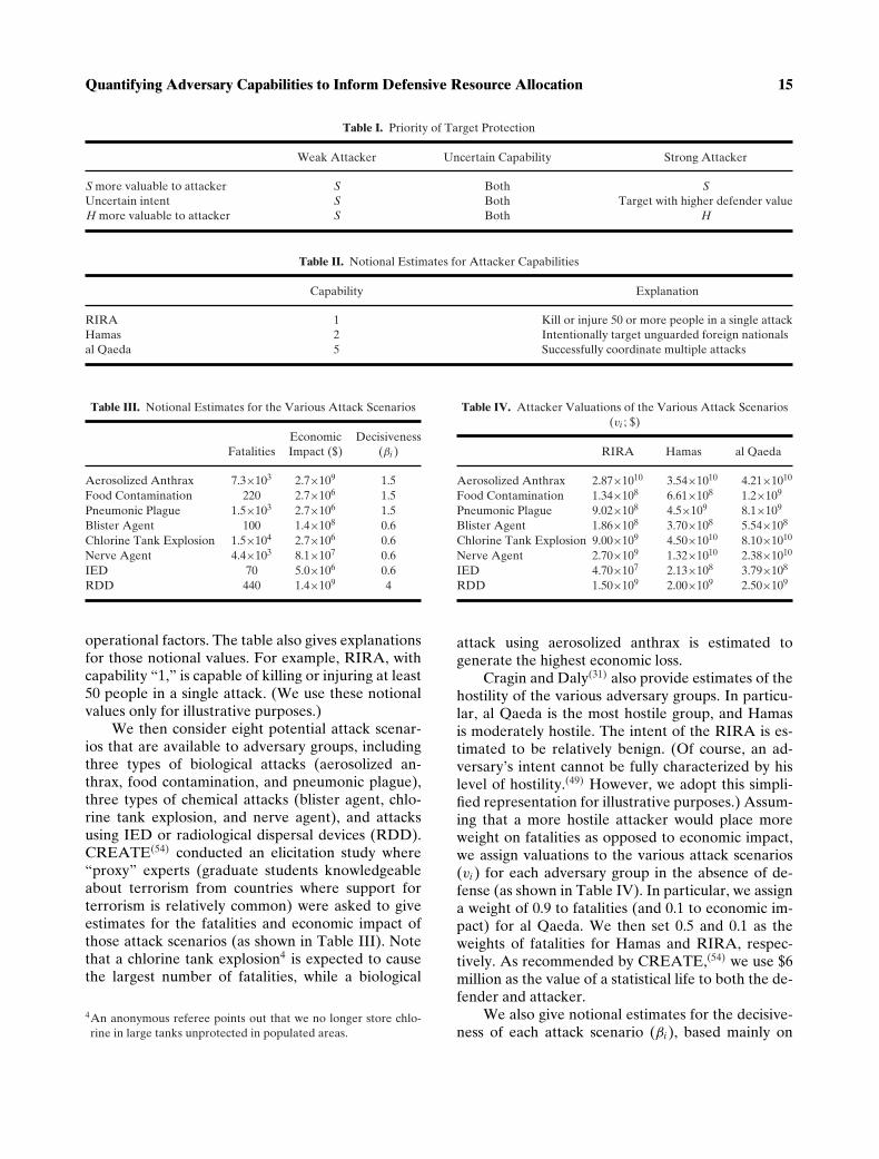
Finally, we present a hypothetical example of ap-plication to illustrate the usability of the proposedgame-theoretic model. We consider three possibleorganizations: Northern Ireland’s Real Irish Repub-lican Army (RIRA);3 the Palestinian group Hamas;and al Qaeda. Cragin and Daly(31) give notional es-timates for the three organizations’ capabilities us-ing a 1–5 rating scale as shown in Table II. Thoseestimates are based on both organizational and

3The Real Irish Republican Army, otherwise known as the RealIRA or RIRA, is a successor to the original Irish RepublicanArmy, which existed from 1922 to 1969.

14 Wang and Bier

Fig. 9. Effects of defender uncertainty about at-tacker intent and capability.

Quantifying Adversary Capabilities to Inform Defensive Resource Allocation 15

Table I. Priority of Target Protection

Weak Attacker Uncertain Capability Strong Attacker

S more valuable to attacker S Both SUncertain intent S Both Target with higher defender valueH more valuable to attacker S Both H

Table II. Notional Estimates for Attacker Capabilities

Capability Explanation

RIRA 1 Kill or injure 50 or more people in a single attackHamas 2 Intentionally target unguarded foreign nationalsal Qaeda 5 Successfully coordinate multiple attacks

Table III. Notional Estimates for the Various Attack Scenarios

Economic DecisivenessFatalities Impact ($) (βi )

Aerosolized Anthrax 7.3×103 2.7×109 1.5Food Contamination 220 2.7×106 1.5Pneumonic Plague 1.5×103 2.7×106 1.5Blister Agent 100 1.4×108 0.6Chlorine Tank Explosion 1.5×104 2.7×106 0.6Nerve Agent 4.4×103 8.1×107 0.6IED 70 5.0×106 0.6RDD 440 1.4×109 4

operational factors. The table also gives explanationsfor those notional values. For example, RIRA, withcapability “1,” is capable of killing or injuring at least50 people in a single attack. (We use these notionalvalues only for illustrative purposes.)

We then consider eight potential attack scenar-ios that are available to adversary groups, includingthree types of biological attacks (aerosolized an-thrax, food contamination, and pneumonic plague),three types of chemical attacks (blister agent, chlo-rine tank explosion, and nerve agent), and attacksusing IED or radiological dispersal devices (RDD).CREATE(54) conducted an elicitation study where“proxy” experts (graduate students knowledgeableabout terrorism from countries where support forterrorism is relatively common) were asked to giveestimates for the fatalities and economic impact ofthose attack scenarios (as shown in Table III). Notethat a chlorine tank explosion4 is expected to causethe largest number of fatalities, while a biological

4An anonymous referee points out that we no longer store chlo-rine in large tanks unprotected in populated areas.

Table IV. Attacker Valuations of the Various Attack Scenarios(vi ; $)

RIRA Hamas al Qaeda

Aerosolized Anthrax 2.87×1010 3.54×1010 4.21×1010

Food Contamination 1.34×108 6.61×108 1.2×109

Pneumonic Plague 9.02×108 4.5×109 8.1×109

Blister Agent 1.86×108 3.70×108 5.54×108

Chlorine Tank Explosion 9.00×109 4.50×1010 8.10×1010

Nerve Agent 2.70×109 1.32×1010 2.38×1010

IED 4.70×107 2.13×108 3.79×108

RDD 1.50×109 2.00×109 2.50×109

attack using aerosolized anthrax is estimated togenerate the highest economic loss.

Cragin and Daly(31) also provide estimates of thehostility of the various adversary groups. In particu-lar, al Qaeda is the most hostile group, and Hamasis moderately hostile. The intent of the RIRA is es-timated to be relatively benign. (Of course, an ad-versary’s intent cannot be fully characterized by hislevel of hostility.(49) However, we adopt this simpli-fied representation for illustrative purposes.) Assum-ing that a more hostile attacker would place moreweight on fatalities as opposed to economic impact,we assign valuations to the various attack scenarios(vi ) for each adversary group in the absence of de-fense (as shown in Table IV). In particular, we assigna weight of 0.9 to fatalities (and 0.1 to economic im-pact) for al Qaeda. We then set 0.5 and 0.1 as theweights of fatalities for Hamas and RIRA, respec-tively. As recommended by CREATE,(54) we use $6million as the value of a statistical life to both the de-fender and attacker.

We also give notional estimates for the decisive-ness of each attack scenario (βi ), based mainly on

16 Wang and Bier

10 20 30 40 50 60

0.0

0.2

0.4

0.6

0.8

1.0

RIRA

Defensive Budget (B)

Opt

imal

Res

ourc

e A

lloca

tion

Aerosol Anthrax

Chlorine Tank Expl.

Nerve Agent

RDD

Pneumonic Plague

10 20 30 40 50 600.

00.

20.

40.

60.

81.

0

Hamas

Defensive Budget (B)

Opt

imal

Res

ourc

e A

lloca

tion

Chlorine Tank Expl.

Aerosol Anthrax

Nerve Agent

Pneumonic PlagueRDD

10 20 30 40 50 60

0.0

0.2

0.4

0.6

0.8

1.0

al Qaeda

Defensive Budget (B)

Opt

imal

Res

ourc

e A

lloca

tion

Chlorine Tank Expl.

Aerosol Anthrax

Nerve AgentPneumonic Plague

(a) (b) (c)

Fig. 10. Optimal defensive resource allocation in the case study.

the descriptive analysis in Falkenrath et al.(55) onthe difficulty of attackers obtaining required mate-rials and the effectiveness of defensive countermea-sures. For example, chemical weapons are relativelyeasy for many nonstate actors to acquire because theprecursor materials are commercially available andweaponization is not difficult. By contrast, biologicalattacks are believed to be more difficult, and hencerequire greater decisiveness. Even though the seedstocks for biological agents are accessible by somenonstate actors, delivery devices are generally diffi-cult to produce. In terms of the effectiveness of coun-termeasures, both chemical and biological attacks aredifficult to identify and prevent in their early stages.However, radiological attacks may be deterred withhigh probability if we install adequate radioactivesensors.

For simplicity, we consider the zero-sum game ofcomplete information where the defender’s objectiveis to minimize the attacker’s expected payoff, andthe attacker can choose only a single attack scenario.Fig. 10 presents the optimal defensive resource allo-cation in the face of each adversary group, as a func-tion of the defensive budget (measured in multiplesof the capability of the least capable adversary groupRIRA).

RIRA is hypothesized to have a low capability,and to weigh economic impact more heavily than fa-talities. Therefore, RIRA is likely to choose an an-thrax attack, since it has a relatively low level of de-cisiveness and can cause large economic damage. Asa result, it is optimal for the defender to focus herprotection against aerosol anthrax attacks conducted

by RIRA, as shown in Fig. 10(a). Of course, as thedefender’s budget increases, she is able to also investin protection against less economically damaging andmore highly decisive attacks, such as RDD.

By contrast, the more hostile adversary groups,Hamas and al Qaeda, are predicted to prefer achlorine tank explosion because it can kill the mostpeople. Accordingly, chlorine tank explosions arealso the priority for protection, as shown in Figs.10(b) and (c). Moreover, a defender with a fixedbudget is able to protect against more attack scenar-ios in total if the adversary group she is facing is theless capable Hamas, rather than al Qaeda.

5. CONCLUSIONS

This article provides a relatively simple game-theoretic model for analyzing the effects of attackerintent and capabilities on both the attacker’s tar-get choices and the defender’s optimal resourceallocations. In particular, we use contest successfunctions to explicitly capture the extent to whichthe success of an attack is attributable to theattacker’s capability (as well as the defensive invest-ment), rather than pure luck. Moreover, our modelallows the effectiveness of attacker capabilities todiffer across targets (e.g., military vs. civilian targets)and attack modes (e.g., IED vs. nuclear attacks), andalso allows for multiple types of attacker capability(such as capital vs. personnel).

This work is an extension of the Bayesian Stack-elberg game of Bier et al.(8) to account for de-fender uncertainty about attacker capabilities rather

Quantifying Adversary Capabilities to Inform Defensive Resource Allocation 17

than just intent. Attackers with scarce resources arelimited in their choices of targets or attack modes be-cause they are likely to succeed only when the targetsor attack modes they choose have low decisiveness.By contrast, strong attackers are more capable ofchoosing targets according to their goals and motiva-tions (i.e., intent), regardless of decisiveness. There-fore, uncertainty about attacker capabilities plays acritical role in making defensive decisions, especiallywhen targets or attack modes have widely differingdecisiveness.

Preliminary results suggest that precise assess-ment of attacker intent might not be necessary ifthe attacker’s capability is highly uncertain. This re-sult could provide practical guidance for determiningthe optimal tradeoff between intelligence collectionon attacker intent versus intelligence collection oncapabilities.

In order to apply the proposed model to real-world homeland security decisions, we must ofcourse develop practical methods to estimate the var-ious input parameters, such as the decisiveness ofeach target or attack mode, and the output elastic-ity for each type of attacker capability. However,these parameters in our model are not directly ob-servable, and thus cannot pass the “clairvoyant test”of Howard.(56) We could estimate them using statisti-cal methods when historical data are available,(28,30)

or rely on expert estimates, for example, by assigninga larger value of decisiveness for hardened militarytargets than that for soft civilian targets.

Another assumption of this study that limits itsgeneral validity is the additivity of individual riskcomponents. This assumption applies only to protec-tion of relatively isolated and dispersed targets. How-ever, in networks of interacting components (such aspower grids,(57) transportation networks,(37) or com-puter networks), there is no simple rule of thumb toidentify the most critical asset(s) without solving aholistic optimization problem.(58) Therefore, the sug-gestions drawn from this study should be taken withcaution when applied to complex systems. Still, webelieve that this article is a first step toward the goalof using game-theoretic models to account for the ef-fects of uncertainty about adversary intent and ca-pabilities on defensive decisions, and provides usefulguidance on the tradeoffs of collecting intelligenceabout intent versus capabilities.

ACKNOWLEDGMENTS

The authors are thankful to the Editor-in-Chief(Tony Cox) and the Area Editor (Seth Guikema)

of Risk Analysis, and three anonymous referees, fortheir insightful comments, which were helpful in im-proving this article. This research was supported bythe U.S. Department of Homeland Security throughthe National Center for Risk and Economic Anal-ysis of Terrorism Events under Grant 2010-ST-061-RE0001. However, any opinions, findings, and con-clusions or recommendations in this document arethose of the authors and do not necessarily reflectviews of the U.S. Department of Homeland Security.

APPENDIX

Proof for Proposition 1. Suppose that the n targetsare rank ordered such that the defender’s (as wellas the attacker’s) valuations of these targets satisfyv1 ≥ v2, . . . ≥ vn > 0. We first give an intuitive expla-nation of the condition in Proposition 1, and thenshow that the condition is both sufficient and neces-sary for deriving the defender’s optimal strategy.

In the absence of any defense, the attacker willattack only target 1 if v1 > vi for i > 1, while ran-domly choosing one of the first K targets to attack ifthey share the same highest value; that is, v1 = vi fori ≤ K and v1 > vi for i > K. If there are K targetsthat share the same highest value, then the defenderneeds to allocate her resources to make the K tar-gets equally attractive to the attacker. There is only aunique way of doing this since the expected payoff ofan attack on each target si (xi , A)vi is strictly decreas-ing in the defensive investment xi (assuming βi > 0).Deviating from that strategy will make some one ofthe K targets less attractive than others, and defen-sive investments on those less attractive targets willbe wasted.

However, as the defender spends more on theK highest valued target(s), eventually they becomeequally attractive to the attacker as the (K + 1)st tar-get. Then additional resources should be spread overthe first K + 1 targets, as well as targets of the samevalue as vK+1, to equalize and reduce their expectedattacker payoff to be no smaller than the value ofany unprotected target. If the defender continues thisprocess until her budget is exhausted, then the con-dition in Proposition 1 is satisfied. By expanding theset of protected targets in this way, the defender isable to defend as many high-valued targets as possi-ble with limited resources.

This condition is sufficient because the defenderis not able to achieve any lower expected loss withthe same level of budget by using a different defen-sive strategy other than the above process. On the

18 Wang and Bier

other hand, the condition is also necessary. If thereexists a target that receives positive protection but isnot the most attractive to the attacker, then the de-fender can always gain profit by spending less on thattarget, and moving the saved effort to more attractivetarget(s). �

Additional Results for Section 2

Lemma A1. Let the n targets be rank ordered suchthat v1 ≥ v2 . . . ≥ vn > 0, and let B(k) (2 ≤ k ≤ n) bethe minimal level of defender budget needed to equal-ize the attractiveness of the k highest-valued targets;that is, such that Aβ1

Aβ1 +(x1)β1v1 = · · · = Aβk

Aβk+(xk)βkvk for

x1 + · · · + xk = B(k). Then B(i) ≤ B( j) for ∀2 ≤ i <

j ≤ n.

Proof. Suppose that the n targets are rank orderedsuch that v1 ≥ v2 . . . vn > 0. Let C(i, j) (2 ≤ i < j ≤n) be the minimal level of defensive budget neededto equalize the attractiveness of the first i targetswith the jth target; that is, such that Aβ1 v1

Aβ1 +(x1)β1= · · · =

Aβi viAβi +(xi )βi

= Aβ j v j

Aβ j +(xj )β j

for x1 + · · · + xi + xj = C(i, j).

Then it is easy to show that B(i) ≤ C(i − 1, j) ≤ B( j)

for 2 ≤ i < j ≤ n. �Corollary A1. If the n targets are rank ordered suchthat v1 ≥ v2 . . . ≥ vn > 0, and B(k) (k = 2, . . . , n) arechosen as in Lemma A1, then the solution (x∗

1 , . . . , x∗n)

to the optimization problem defined by Equations (1),(2), and (3) satisfies one of the following cases:

(i) If B > B(n), then x∗i > 0 for ∀i = 1, . . . , n;

(ii) If B(k) < B ≤ B(k+1) (2 ≤ k ≤ n − 1), thenx∗

i > 0 for ∀i ≤ k and x∗i = 0 for ∀i > k;

(iii) If 0 < B ≤ B(2), then x∗1 > 0 and x∗

i = 0 for∀i > 1.

Proof. This corollary follows directly from the dis-cussion in the proof for Proposition 1. �Proof for Proposition 2. Recall that for any given xand A, the likelihood of target choice pi (x, A, v) isgiven by:

pi (x, A, v) ={

1Z if i ∈ arg max j s j (xj , A)v j

0 otherwise ,

where Z is the cardinality of the set { j :arg max j s j (xj , A)v j }. The attacker’s expectedpayoff given x and Acan then be calculated as givenby: ∑n

i=1 pi (x, A, v)si (xi , A)vi

= ∑i∈arg max j s j (xj ,A)v j

1Zsi (xi , A)vi

= max j s j (xj , A)v j .

Therefore, we have the following:

minx1+···+xn≤B

∫ n∑i=1

pi (x, A, v)si (xi , A)vi dFA(A)

= minx1+···+xn≤B

∫max

j{s j (xj , A)v j }dFA(A). �

We then prove the first-order necessary con-dition. For convenience, we denote l(x, A) =max j s j (xj , A)v j and L(x) = ∫

l(x, A)dFA(A). Weare interested in:

L(x + tei ) − L(x)=∫

l(x + tei , A) − l(x, A)dFA(A),

(A.1)

where t > 0 and ei is the ith unit coordinate vector.Suppose that for any given defensive strategy x, theset { j : arg max j s j (xj , A)v j } is a singleton with prob-ability one under the distribution FA(·). If we denoten∗(x, A) = arg max j s j (xj , A)v j , then with probabil-ity one the following inequality holds:

sn∗(xn∗ , A)vn∗ > si (xi , A)vi for ∀i = n∗.

Note that si (xi , A)vi is continuous and strictly in-creasing in xi for all i . Therefore, ∃t̄ > 0 such that for∀0 < t < t̄ , we have:

sn∗(xn∗ + t, A)vn∗ > si (xi , A)vi and

sn∗(xn∗ , A)vn∗ > si (xi + t, A)vi for ∀i = n∗.

So, l(x + tei , A) = sn∗(xn∗ + t · 1{i=n∗}, A)vn∗ for i =1, . . . , n with probability one, where 1{i=n∗} equals 1 ifi = n∗ and 0 otherwise. Take such t̄ and for 0 < t < t̄rewrite Equation (A.1) as given by:

L(x + tei ) − L(x) =∫

sn∗(xn∗ + t · 1{i=n∗}, A)vn∗

−sn∗(xn∗ , A)vn∗dFA(A). (A.2)

By dividing both sides of Equation (A.2) and takingthe limit at t → 0, we have the following equation:

limt→0

L(x + tei ) − L(x)t

=∫

limt→0

sn∗ (xn∗ + t · 1{i=n∗}, A)vn∗ − sn∗ (xn∗ , A)vn∗

tdFA(A).

Equivalently,

dL(x)dxi

=∫

gi (x, A)dFA(A),

Quantifying Adversary Capabilities to Inform Defensive Resource Allocation 19

where

gi (x, A) ={

∂

∂xn∗ sn∗ (xn∗ , A)vn∗ if i = n∗

0 if i = n∗.

Finally, since the defender’s objective functionL(x) is strictly decreasing in xi for all i , the to-tal budget B needs to be exhausted at optimality.The Karush-Kuhn-Tucker (KKT) condition for aninterior-point solution to the optimization problemminx1+···+xn=B L(x) is then given by dL(x)

dxi= μ for all

i = 1, . . . , n, with xi > 0 and x1 + · · · + xn = B.For given defensive resource allocation x =

(x1, . . . , xn) and the attacker’s allocation of effort a =(a1, . . . , an), we consider two cases. First, if ai > 0 anda j = 0 for i = j , and the marginal expected attackerpayoffs of attacking targets i and j satisfy:

hi (xi , ai ) < h j (xj , a j ),

then the defender can gain additional benefits by re-ducing a small portion ε > 0 from the effort devotedto target i , and spending it on target j . In particular,the difference between the attacker’s total expectedpayoffs before and after the reallocation is given by:

[si (xi , ai )vi + s j (xj , a j )v j ]

− [si (xi , ai − ε)vi + s j (xj , a j + ε)v j ]

= si (xi , ai )vi − si (xi , ai − ε)vi

+ s j (xj , a j )v j − s j (xj , a j + ε)v j

= hi (xi , ai )ε + h j (xj , a j )(−ε) + o(ε)

= [hi (xi , ai ) − h j (xj , a j )] ε + o(ε),

where o(ε) is the first-order Taylor remainder. Sincehi (xi , ai ) < h j (xj , a j ), the above equation is strictlysmaller than zero for sufficiently small ε. �

On the other hand, if ai > 0 and a j > 0 for i = j ,and hi (xi , ai ) < h j (xj , a j ), then the defender can alsogain profit by reducing a small portion ε > 0 from theeffort devoted to target i and spending it on target j .

Therefore, the condition in Proposition 3 isnecessary.

Derivation of Results in Example 1

We focus on the case where AB < ( v1

v2− 1)−1/β .

For convenience, we denote R = AB and r = x1

B , andthen investigate the relationship between R and r asgiven by:

Rβ + rβ

Rβ + (1 − r)β= v1

v2.

By rearranging the above equation, we get an implicitfunction of r and R as given by:

z(r, R) = (1 − r)βv1 − rβv2 − Rβ(v2 − v1) = 0.

We then apply the implicit function theorem, and ob-tain the first-order derivative of r with respect to R,as given by:

drdR

= −∂z/∂ R∂z/∂r

= Rβ−1(v1 − v2)(1 − r)β−1 + rβ−1

> 0,

for R > 0 and 0 < r < 1. Note that we assume v1 >

v2, so the optimal proportion of defensive investmentallocated to target 1, r∗ = x∗

1B , is strictly increasing

with the attacker’s capability advantage R = AB .

REFERENCES

1. Bellavita C. Changing homeland security: Twelve questionsfrom 2009. Homeland Security Affairs, 2010; 6:Article 1.

2. Department of Homeland Security, Risk Steering Committee.DHS Risk Lexicon. Washington, DC: Department of Home-land Security, 2008.

3. Willis HH, Morral AR, Kelly TK, Medby JJ. 2005 Estimat-ing Terrorism Risk. Santa Monica, CA: RAND Corporation,2005.

4. Parnell GS, Borio LL, Brown GG, Banks D, Wilson AG. Sci-entists urge DHS to improve bioterrorism risk assessment.Biosecurity and Bioterrorism: Biodefense Strategy, Practice,and Science, 2008; 6(4):353–356.

5. Cox LA Jr. Some limitations of “risk = threat × vulnerabil-ity × consequence” for risk analysis of terrorist attacks. RiskAnalysis, 2008; 28(6):1749–1761.

6. Brown G, Cox LA Jr. How probabilistic risk assessmentcan mislead terrorism risk analysts. Risk Analysis, 2011;31(2):196–204.

7. National Research Council, Committee to Review the Depart-ment of Homeland Security’s Approach to Risk Analysis. Re-view of the Department of Homeland Security’s Approach toRisk Analysis. Washington, DC: National Academies Press,2010.

8. Bier VM, Oliveros S, Samuelson L. Choosing what to protect.Journal of Public Economic Theory, 2007; 9(4):563–587.

9. Bier VM, Nagaraj A, Abhichandani V. Optimal allocation ofresources for defense of simple series and parallel systemsfrom determined adversaries. Reliability Engineering and Sys-tem Safety, 2005; 87:313–323.

10. Patcha A, Park JM. A game theoretic formulation for intru-sion detection in mobile ad hoc networks. International Jour-nal of Network Security, 2006; 2(2):131–137.

11. Hausken K, Bier VM Zhuang. Defending against terrorism,natural disaster, and all hazards. Pp. 65-97 in Bier VM, AzaiezMN (eds). Game Theoretic Risk Analysis of Security Threats.New York: Springer, 2009.

12. Zhuang J, Bier VM. Balancing terrorism and natural disasters:Defensive strategy with endogenous attacker effort. Opera-tions Research, 2007; 55(5):976–991.

13. Pita J, Bellamane H, Jain M, Kiekintveldt C, Tsai J, OrdonezF, Tambe M. Security applications: Lessons of real-world de-ployment. ACM SIGecom Exchanges, 2009; 8(2):Article 5.

14. Paruchuri P, Pearce J, Marecki J, Tambe M, Ordonez F, KrausS. Playing games with security: An efficient exact algorithm for

20 Wang and Bier

solving Bayesian Stackelberg games. Pp. 895–902 in AAMAS-2008 Conference, Estoril, Portugal, 2008.

15. National Research Council, Committee on MethodologicalImprovements to the Department of Homeland Security’sBiological Agent Risk Analysis. Department of HomelandSecurity Bioterrorism Risk Assessment: A Call for Change.Washington, DC: National Academies Press, 2008.

16. Zhuang J, Bier VM. Reasons for secrecy and deception inhomeland-security resource allocation. Risk Analysis, 2010;30(12):1737–1743.

17. Government Accountability Office. Homeland Security: DHSRisk-Based Grant Methodology Is Reasonable, But CurrentVersion’s Measure of Vulnerability Is Limited. GAO-08-852.U.S. Government Accountability Office, 2008.

18. Farrow S. The economics of homeland security expenditures:Foundational expected cost-effectiveness approaches. Con-temporary Economic Policy, 2007; 25(1):14–26.

19. Willis HH. Guiding resource allocations based on terrorismrisk. Risk Analysis, 2007; 27(3):597–606.

20. Keeney RL, von Winterfeldt D. A value model for evaluatinghomeland security decisions. Risk Analysis, 2011; 31(9):1470–1487.

21. Skaperdas S. Contest success functions. Economic Theory,1996; 7(2):283–290.

22. Tullock G. Efficient rent seeking. Pp. 97–112 in Buchanan JM,Tollison RD, Tullock G (eds). Toward a Theory of the Rent-Seeking Society. College Station, TX: Texas A&M UniversityPress, 1980.

23. Hirshleifer J, Osborne E. Truth, effort, and the legal battle.Public Choice 2001; 108:169–195.

24. Szymanski S. The economic design of sporting contests. Jour-nal of Economic Literature, 2003; 41:1137–1187.

25. Garfinkel MR, Skaperdas S. Economics of conflict: Anoverview. Pp. 649–709 in Hartley K, Sandler T (eds). Hand-book of Defense Economics, Vol. 2. Amsterdam: Elsevier,2007.

26. Levitin G, Hausken K. Resource distribution in multiple at-tacks against a single target. Risk Analysis, 2010; 1231–1239.

27. Hausken K, Bier VM. Defending against multiple differentattackers. European Journal of Operational Research, 2011;211:370–384.

28. Hwang SH. Contest success functions: Theory and evi-dence. Working Papers, 2009-04. University of MassachusettsAmherst, Department of Economics, 2009. Available at:http://ideas.repec.org/p/ums/papers/2009-04.html.

29. Hirshleifer J. The technology of contract as an economic ac-tivity. American Economic Review, 1991; 81(2):130–134.

30. Rotte R, Schmidt CM. On the production of victory: Empiricaldeterminants of battlefield success in modern war. IZA Dis-cussion Papers, 491. Institute for the Study of Labor (IZA),2002. Available at http://ideas.repec.org/p/iza/izadps/dp491.html.

31. Cragin RK, Daly SA. The Dynamic Terrorist Threat: An As-sessment of Group Motivations and Capabilities in a ChangingWorld. Santa Monica, CA: RAND Corporation, 2004.

32. Lanchaster FW. Mathematics in warfare. Pp. 2138–2157 inNewman JR (ed). The World of Mathematics. New York:Simon and Shuster, 1956.

33. Hughes WP. A salvo model of warships in missile combatused to evaluate their staying power. Naval Research Logis-tics, 1995; 42:267–289.

34. Lucas TW. The stochastic versus deterministic argument forcombat simulations: Tales of when the average won’t do. Mil-itary Operations Research, 2000; 5(3):9–28.

35. Armstrong MJ. A stochastic salvo model for naval surfacecombat. Operations Research, 2005; 53(5):830–841.

36. Powell R. Defending against terrorist attacks with limited re-sources. American Political Science Review, 2007; 101(3):527–541.

37. Brown G, Matthew C, Salmeron J, Wood K. Defending criticalinfrastructure. Interfaces, 2006; 36(6):530–544.

38. Brown G, Carlyle M, Diehl D. Kline J, Wood K. A two-sidedoptimization for theater ballistic missile defense. OperationsResearch, 2005; 53(5):745–763.

39. Brown G, Carlyle M, Abdul-Ghaffar A, Kline J. A defender-attacker optimization of port radar surveillance. Naval Re-search Logistics, 2011; 58:223–235.

40. Brown G, Kline J, Thomas A, Washburn A, Wood K. A game-theoretic model for defense of an oceanic bastion againstsubmarines. Military Operations Research, 2011; 16(4):25–40.

41. Willis HH. Challenges of Applying Risk Management to Ter-rorism Security Policy. Santa Monica, CA: RAND Corpora-tion, 2008.

42. Bier VM. Choosing what to protect. Risk Analysis, 2007;27(3):607–620.

43. Lapan HE, Sandler T. Terrorism and signaling. EuropeanJournal of Political Economy, 1993; 9(3):383–397.

44. Dupuy TN. Attrition: Forecasting Battle Casualties andEquipment Losses in Modern War. Falls Church, VA: NovaPublications, 1995.

45. Rai BK, Sarin R. Generalized contest success functions. Eco-nomic Theory, 2007; 40(1):139–149.

46. Yuille AL, Rangarajan A. The concave-convex procedure(CCCP). Neural Computation, 2003; 15(4):915–936.

47. Rios LM, Sahinidis NV. Derivative-free optimization: A re-view of algorithms and comparison of software implemen-tations. Journal of Global Optimization, 2013; 56(3):1247–1293.

48. Wang C. Methods development for optimal defense againstadaptive adversaries: Quantification of uncertain prefer-ences and development of computational approaches. The-sis, University of Wisconsin–Madison, Ann Arbor, MI[ProQuest/UMI, 2013].

49. Rosoff H, John R. Decision analysis by proxy for the ratio-nal terrorist. Proceedings of the 21st International Joint Con-ference on Artificial Intelligence, Workshop on QuantitativeRisk Analysis for Security Applications, 2009.

50. Be a Hero, Hug a Terrorist. Operations Research & Manage-ment Science Today: News. April 19, 2006. http://www.orms-today.org/enews/fr0406e.html.

51. Douglas PH. The Cobb-Douglas production function onceagain: Its history, its testing, and some new empirical values.Journal of Political Economy, 1976; 84(5):903–916.

52. Wang C, Bier VM. Target-hardening decisions based on un-certain multiattribute terrorist utility. Decision Analysis, 2011;8(4):286–302.

53. Bier VM, Menoyo JB, Wang C. Achieving realistic levelsof defensive hedging based on non-monotonic and multi-attribute terrorist utility functions. Pp. 125–139 in HerrmannJ (ed). Handbook of Operations Research, Homeland Se-curity and Emergency Preparedness. New York: Springer,2013.

54. Center for Risk and Economic Analysis of Terrorism Events.Adaptive Adversary Modeling for Terrorism Risk Analy-sis: Final Report. Los Angeles, CA: University of SouthernCalifornia, 2011.

55. Falkenrath RA, Newman RD, Thayer BA. American’sAchilles’ Heel. Cambridge, MA: MIT Press, 1998.

56. Howard RA. Decision analysis: Practice and promise. Man-agement Science, 1988; 34(6):679–695.

57. Salmeron J, Wood K, Baldick R. World-case interdiction anal-ysis of large-scale electric power grids. IEEE Transactions onPower Systems, 2009; 24:96–104.

58. Alderson DL, Brown GG, Carlyle WM. Sometimes there isno “most-vial” arc: Assessing and improving the operationalresilience of systems. Military Operations Research, 2013;18(1):21–37.