Quantifying Inefficiency in Cost-Sharing Mechanisms∗

Tim Roughgarden† Mukund Sundararajan‡

February 26, 2009

Abstract

In a cost-sharing problem, several participants with unknown preferences vie to receive somegood or service, and each possible outcome has a known cost. A cost-sharing mechanism is aprotocol that decides which participants are allocated a good and at what prices. Three desirableproperties of a cost-sharing mechanism are: incentive-compatibility, meaning that participantsare motivated to bid their true private value for receiving the good; budget-balance, meaningthat the mechanism recovers its incurred cost with the prices charged; and economic efficiency,meaning that the cost incurred and the value to the participants are traded off in an optimalway. These three goals have been known to be mutually incompatible for thirty years. Nearly allthe work on cost-sharing mechanism design by the economics and computer science communitieshas focused on achieving two of these goals while completely ignoring the third.

We introduce novel measures for quantifying efficiency loss in cost-sharing mechanismsand prove simultaneous approximate budget-balance and approximate efficiency guarantees formechanisms for a wide range of cost-sharing problems, including all submodular and Steinertree problems. Our key technical tool is an exact characterization of worst-case efficiency lossin Moulin mechanisms, the dominant paradigm in cost-sharing mechanism design.

1 Introduction

1.1 Mechanism Design

In the past decade, there has been a proliferation of large systems used and operated by independentagents with competing objectives (most notably the Internet). Motivated by such applications, anincreasing amount of algorithm design research studies optimization problems that involve self-interested entities. Naturally, game theory and economics are important for modeling and solvingsuch problems. Mechanism design is a classical area of microeconomics that has been particularlyinfluential. The field of mechanism design studies how to solve optimization problems in whichpart of the problem data is known only to self-interested players. It has numerous applications to,for example, auction design, pricing problems, and network protocol design [17, 22, 32, 38].

∗Preliminary versions of these results appeared in the Proceedings of the 38th Annual Symposium on Theory

of Computing, May 2006, and Proceedings of the 12th Conference on Integer Programming and Combinatorial

Optimization, June 2007.†Department of Computer Science, Stanford University, 462 Gates Building, 353 Serra Mall, Stanford, CA 94305.

Supported in part by ONR grant N00014-04-1-0725, DARPA grant W911NF-05-1-0224, an NSF CAREER Award,

and an Alfred P. Sloan Fellowship. Email: tim@cs.stanford.edu.‡Department of Computer Science, Stanford University, 470 Gates Building, 353 Serra Mall, Stanford, CA 94305.

Supported in part by ONR Grants N00014-01-1-0795 and N00014-04-1-0725. Email: mukunds@cs.stanford.edu.

1

Selling a single good to one of n potential buyers is a paradigmatic problem in mechanismdesign. Each bidder i has a valuation vi, expressing its maximum willingness to pay for the good.We assume that this value is known only to the bidder, and not to the auctioneer. A mechanism forselling a single good is a protocol that determines the winner and the selling price. Each bidder iis “selfish” in that it wants to maximize its “net gain” (vi − p)xi from the auction, where p is theprice, and xi is 1 if the bidder wins and 0 if the bidder loses.

What optimization problem underlies a single-good auction? One natural goal is economicefficiency, which in this context demands that the good is sold to the bidder with the highestvaluation. This goal is trivial to accomplish if the valuations are known a priori. Can it beachieved when the valuations are private?

Vickrey [43] provided an elegant solution. First, each player submits a sealed bid bi to the seller,which is a proxy for its true valuation vi. Second, the seller awards the good to the highest bidder.This achieves the efficient allocation if we can be sure that players bid their true valuations—ifbi = vi for every i. To encourage players to bid truthfully, we must charge the winner a non-zeroprice. (Otherwise, all players will bid gargantuan amounts in an effort to be the highest.) On theother hand, if we charge the winning player its bid, it encourages players to underbid. (Biddingyour maximum willingness to pay ensures a net gain of zero, win or lose.) Vickrey [43] suggestedcharging the winner the value of the second-highest bid, and proved that this price transformstruthful bidding into an optimal strategy for each bidder, independent of the bids of the otherplayers. In turn, the Vickrey auction is guaranteed to produce an efficient allocation of the good,provided all players bid in the obvious, optimal way.

1.2 Cost-Sharing Mechanisms

The revenue obtained by a mechanism can be as or more important than its economic efficiency,especially in settings where the mechanism designer incurs a non-trivial cost, such as productioncosts. This issue motivates the study of cost-sharing mechanisms that guarantee sufficient revenueto cover the incurred costs. Moulin and Shenker [36] describe a range of applications of cost-sharing mechanisms across economics, and Feigenbaum, Papadimitriou, and Shenker [16] motivatethe study of such mechanisms from a computer networking perspective.

Formally, a cost-sharing problem is defined by a set U of players vying to receive some goodor service, and a cost function C : 2U → R+ describing the cost incurred by the mechanism as afunction of the auction outcome — the set S of winners. We assume that C(∅) = 0 and that Cis nondecreasing (i.e., S ⊆ T implies C(S) ≤ C(T )). We impose no explicit limit on the numberof winners, but a large number of winners might result in extremely large costs. The problem ofselling a single good can be viewed as the special case in which C(S) = 0 if |S| ≤ 1 and C(S) = +∞otherwise. A more complex example is a Steiner tree cost-sharing problem, where U represents aset of potential clients, located in an undirected graph with fixed edge costs, that want connectivityto a server t [16, 24]. In this application, C(S) denotes the cost of connecting the terminals in Sto t — the cost of the minimum-cost Steiner tree that spans S ∪ t. For a cost function C anda valuation profile vii∈U , the efficient allocation is the subset that maximizes the social welfare:W (S) = v(S) − C(S), where v(S) denotes

∑

i∈S vi.For a given set U and function C, a cost-sharing mechanism is a protocol that decides which

players win and at what prices. Typically, such a mechanism is also (perhaps approximately)budget-balanced, meaning that the cost incurred is passed on to the auction’s winners. Budget-balanced cost-sharing mechanisms provide control over the revenue generated, relative to the cost

2

incurred by the mechanism designer.Summarizing, we have identified three natural goals in cost-sharing mechanism design: incentive-

compatibility, meaning that every player’s optimal strategy is to bid its true private value vi forreceiving the service; budget-balance, meaning that the mechanism recovers its incurred cost withthe prices charged; and efficiency, meaning that the cost and valuations are traded off in an optimalway.

Unfortunately, roughly thirty years ago Green, Kohlberg, and Laffont [18] and Roberts [40] ruledout the existence of mechanisms that simultaneously satisfy these three constraints, even in verysimple cost-sharing problems. This impossibility result motivates relaxing at least one of theseproperties. Until recently, nearly all work in cost-sharing mechanism design completely ignoredeither budget-balance or efficiency. Without the budget-balance constraint, there is an extremelypowerful and flexible mechanism that is incentive-compatible and efficient: the VCG mechanism(see e.g. [16, 36]). This mechanism specializes to the Vickrey auction when selling a single good,but it is far more general. The VCG mechanism is typically not approximately budget-balancedfor any reasonable approximation factor (assuming “individually rational” prices, see e.g. [15] fordetails).

A second approach is to discard economic efficiency as an objective and insist on incentive-compatibility and budget-balance. Until very recently [33], the only general technique for de-signing mechanisms of this type was due to Moulin [35]. Researchers have developed numerousapproximately budget-balanced Moulin mechanisms for cost-sharing problems arising from dif-ferent combinatorial optimization problems, including fixed-tree multicast problems [2, 15, 16];more general submodular problems [35, 36]; scheduling problems [6, 8]; network design prob-lems [19, 20, 24, 25, 27, 29, 39]; facility location problems [30, 39]; and various covering prob-lems [12, 23]. With one exception discussed below, none of these works provided any guaranteeson the economic efficiency achieved by the proposed mechanisms.

1.3 Why Quantify Inefficiency?

Impossibility results are, of course, common in optimization. Motivated by conditional impossibilityresults like Cook’s Theorem [10], as well as information-theoretic lower bounds in restricted modelsof computation like online [7] and streaming algorithms [37], algorithm designers are accustomed todevising heuristics and proving worst-case guarantees about them using approximation measures.This approach can also be applied to cost-sharing mechanism design to quantify the inevitableefficiency loss in incentive-compatible, budget-balanced cost-sharing mechanisms. As worst-caseapproximation measures are rarely used in economics, this research direction has not been pursuedpreviously.

Quantifying efficiency loss in cost-sharing mechanisms is an important goal for several rea-sons. First, a quantitative approximation measure is necessary to rigorously compare the economicefficiency of different mechanisms for a cost-sharing problem, and to identify a mechanism as “op-timally efficient” subject to budget-balance constraints. Second, such a measure allows us to defineand compare the intrinsic complexity of cost-sharing problems. To give an analogy, recall that the“difficulty” of an NP-hard optimization problem is often identified with the best-possible approx-imation ratio achievable by a polynomial-time algorithm for it, assuming P 6= NP (see e.g. [3]).For a cost-sharing problem, we can similarly interpret the efficiency guarantee achieved by an opti-mally efficient mechanism as a measure of the problem’s “complexity”. Third, even when economicefficiency is not the primary objective, requiring “reasonable” (but not necessarily optimal) effi-

3

ciency can be useful for constraining the mechanism design space. For example, the intuitively“undesirable” family of mechanisms identified by Immorlica, Mahdian, and Mirrokni [23, Example4.1], which stubbornly satisfy a long list of standard mechanism design requirements, admit nonon-trivial efficiency guarantees.

The sole previous work on quantifying efficiency loss in budget-balanced cost-sharing mecha-nisms is by Moulin and Shenker [36], who studied submodular cost-sharing problems and an additivenotion of efficiency loss. Their results successfully rank different fully budget-balanced mechanismsfor an arbitrary but fixed submodular cost-sharing problem according to worst-case efficiency loss(see also Section 4). However, it is not obvious how to use their efficiency loss measure to makecomparisons between different cost-sharing problems. Additionally, the approach in [36] has notyet been extended beyond submodular cost-sharing problems, and most of the problems studied inthe computer science literature fall outside of this class [6, 8, 19, 20, 23, 24, 25, 27, 29, 30, 39].

1.4 How to Quantify Inefficiency?

The impossibility results in [18, 40] motivate approximate notions of budget-balance and economicefficiency. In this paper, we define a mechanism to be β-budget-balanced for a parameter β ≥ 1 ifthe sum of the prices charged is always at least the cost incurred and is also at most β times thiscost. Several previous works instead require that the revenue is no more than and at least a 1/βfraction of the incurred cost; we obtain similar results for this alternative definition (see Sections 1.7and 6).

Several definitions of approximate efficiency are possible. Arguably, the most natural require-ment is to insist that a mechanism always computes an outcome S that is a ρ-approximation of thesocial welfare: W (S) ≥ ρ · W (S∗), where S∗ is the economically efficient solution. Unfortunately,Feigenbaum et al. [15] shattered any hope for such a guarantee, even in very simple cost-sharingproblems: for every β ≥ 1 and β-budget-balanced incentive-compatible mechanism, there is a valu-ation profile such that the efficient solution has strictly positive welfare but the mechanism producesthe empty outcome (with zero welfare). Thus every mechanism, no matter how intuitively “good”or “bad”, is a 0-approximation algorithm for the social welfare objective. This inapproximabilityresult is characteristic of mixed-sign objective functions such as the social welfare.

We must therefore measure efficiency loss in a different way. Our basic efficiency guaranteeshave the following form, for a parameter ρ ≥ 0 and a mechanism for the cost-sharing problem C:for every valuation profile,

W (S∗) − W (S) ≤ ρ · C(S∗), (1)

where S is the output of the mechanism and S∗ is an efficient outcome. In this case, we call themechanism ρ-approximate.

We have chosen to present this efficiency guarantee in terms of additive welfare loss, but it isrobust and admits several different interpretations. For example, the bound in (1) implies a relativeapproximation guarantee for a different formulation of economic efficiency. Precisely, define thesocial cost π(S) of an outcome S to be the cost incurred by the mechanism plus the sum of theexcluded valuations (i.e., opportunity cost):

π(S) = C(S) + v(U \ S). (2)

Since social cost and social welfare are related by the affine transformation π(S) = −W (S)+ v(U),minimizing the social cost is ordinally equivalent to maximizing the social welfare. The two objective

4

functions are not, of course, equivalent from an approximation perspective. Indeed, while theimpossibility result in Feigenbaum et al. [15] precludes any relative approximation of the socialwelfare, every ρ-approximate cost-sharing mechanism also (ρ + 1)-approximates the social cost.Such non-approximation-preserving transformations are common in applications with mixed-signobjective functions, including prize-collecting combinatorial optimization problems (e.g. [5]) anddiscrete maximum-likelihood problems (e.g. [28]).

A second interpretation of the bound in (1) is motivated by the examples used in the impossi-bility result in [15]. These examples are intuitively difficult because the optimal outcome S∗ haslarge cost C(S∗) and value v(S∗) only slightly larger than C(S∗), leaving the mechanism with no“margin for error”. Can we obtain a relative approximation of welfare when the value of an optimaloutcome is bounded away from its cost? To formalize this question, we say that an outcome S isη-separated if W (S) ≥ η ·C(S) or, equivalently, if v(S) ≥ (η + 1) ·C(S). The punchline, proved viaa simple calculation, is this: if a mechanism is ρ-approximate, then ρ is the separation thresholdbeyond which non-trivial welfare approximation is possible. Precisely, a ρ-approximate mechanismextracts at least a (1−ρ/η) fraction of the optimal welfare when the optimal outcome is η-separated.

1.5 Our Techniques: Moulin Mechanisms and Summability

Our overarching goal is to identify tight upper and lower bounds on the best-possible efficiency guar-antees of incentive-compatible and budget-balanced mechanisms for a wide range of cost-sharingproblems. Our first contribution is a general analytical framework for proving such bounds (Sec-tion 3). The framework applies to Moulin mechanisms, the dominant paradigm in budget-balancedcost-sharing mechanism design.

Roughly, a Moulin mechanism simulates an ascending iterative auction. In each iteration, aprice χ(i, S) is offered to each player i of the remaining players S. Players that accept remainin contention; the others are removed. The mechanism halts when all remaining players acceptthe prices offered to them. To achieve approximate budget-balance, the mechanism offers pricesat each iteration that approximately cover the cost that would be incurred if the iteration is thelast. To obtain incentive-compatibility, a Moulin mechanism offers each player a non-decreasingsequence of prices. The function χ is called a cost-sharing method, and it uniquely defines thecorresponding Moulin mechanism. (See Section 2 for formal definitions.) Until very recently,almost all approximately budget-balanced cost-sharing mechanisms were Moulin mechanisms [6, 8,19, 20, 23, 24, 25, 27, 29, 30, 36, 39], with the mechanisms of Devanur, Mihail, and Vazirani [12]forming a notable exception.

Our first main result is a characterization of the worst-case efficiency loss of a Moulin mechanismin terms of a single parameter of its underlying cost-sharing method. Given a cost-sharing methodχ and a cost function C defined over the same set U of players, this parameter α is easy to describe.We say that the method χ is α-summable for C if the following condition holds for every subsetS ⊆ U and every ordering of the players of S:

|S|∑

ℓ=1

χ(iℓ, Sℓ) ≤ α · C(S), (3)

where iℓ and Sℓ denote the ℓth player and the set of the first ℓ players in the ordering, respectively.In other words, start with the empty set, add players of S one-by-one according to the givenordering, and let Xℓ denote the cost share of the ℓth player (according to χ) when the player is

5

first added. The cost-sharing method χ is α-summable for C if the sum∑

ℓ Xℓ only overestimatesthe cost of C(S) by an α factor (for a worst-case choice of the subset S and the ordering of theplayers).

For example, in the special case of a symmetric cost function and equal cost shares, summabilityis a measure of the “amount of concavity” of the cost function. Consider the function C(S) = |S|dfor d ∈ [0, 1] on the universe U = 1, 2, . . . , n and the cost-sharing method χ(i, S) = C(S)/|S| =|S|d−1. The summability of χ is then determined by the set S = U ; the ordering σ is irrelevant.A simple calculation shows that this summability is roughly 1/d for fixed d > 0 and large n, andgrows as ln n when d = 0.

We prove that summability characterizes approximate efficiency in the following sense: a Moulinmechanism is (α−1)-approximate if and only if its underlying cost-sharing method is α-summable.The key idea behind our proof is to view a Moulin mechanism as a greedy descent algorithmwith respect to a type of “potential function”. Summability then arises naturally as a measure ofproximity between this potential function and the social objective function.

1.6 Our Results: Efficiency Guarantees for Submodular and Steiner Tree Prob-

lems

Bounding the summability (3) of a cost-sharing method is a non-trivial but often tractable problem.We demonstrate this by applying our summability framework to obtain matching upper and lowerbounds on the best-possible efficiency guarantees of Moulin mechanisms for two widely studiedclasses of cost-sharing problems, submodular problems (Section 4) and Steiner tree problems (Sec-tion 5). Since the conference version of this work [41], many more applications have been found;see Section 7.

A submodular cost-sharing problem is defined by a player set U and a nondecreasing costfunction C such that, for every S1 ⊆ S2 and i /∈ S2,

C(S2 ∪ i) − C(S2) ≤ C(S1 ∪ i) − C(S1). (4)

Submodular cost-sharing problems admit a range of budget-balanced Moulin mechanisms [25, 36].One is the Shapley mechanism [16, 36], whose underlying cost-sharing method is derived fromthe Shapley value. As a first application of our framework, we prove that for every submodularcost-sharing problem, the corresponding Shapley cost-sharing method is Hk-summable, where kis the number of players served in an optimal solution, and Hk =

∑

i≤k 1/i ≈ ln k denotes thekth Harmonic number. Our characterization result then implies that the Shapley mechanism is(Hk − 1)-approximate and also Hk-approximates the social cost for every submodular cost-sharingproblem. It also implies that the Shapley mechanism is an optimal Moulin mechanism in thefollowing sense: there is a simple submodular cost-sharing problem for which every budget-balancedMoulin mechanism is at least Hk-summable. These results reprove, from a different perspective,earlier results of Moulin and Shenker [36, Proposition 2].

Our most mathematically involved results concern the much more complex class of Steiner treecost-sharing problems. Such problems are generally not submodular, and no efficiency guarantees ofany sort were previously known for approximately budget-balanced mechanisms for such problems.Our main positive result is a proof that the 2-budget-balanced Steiner tree cost-sharing methoddesigned by Jain and Vazirani [24] is O(log2 k)-summable, where k is again the number of playersserved in an optimal solution, and thus the corresponding Moulin mechanism (the JV mechanism)

6

is O(log2 k)-approximate. Our proof blends ideas inspired by online algorithms, primal-dual ap-proximation algorithms, and our analysis for submodular cost functions. Techniques from onlineanalysis are useful because summability is defined in terms of a worst-case player ordering; primal-dual arguments arise because the JV mechanism is based on Edmonds’s primal-dual branchingalgorithm [14].

Our efficiency guarantee for the JV mechanism is weaker than that for the Shapley mechanism,and this is no accident: we use our characterization result and a recursive construction to prove thatevery O(1)-budget-balanced Moulin mechanism for Steiner tree cost-sharing problems is Ω(log2 k)-approximate. Our positive results for submodular problems and this lower bound expose a non-trivial, latent approximation hierarchy among different cost-sharing problems. Of course, thislower bound for Steiner tree problems trivially carries over to the more general network designcost-sharing problems studied in [19, 20, 29, 39].

1.7 Our Results: Budget-Balance vs. Efficiency Trade-Offs

Finally, in Section 6 we extend our summability framework to quantify trade-offs between budget-balance and economic efficiency in cost-sharing mechanisms. In particular, inefficiency can bepartially mitigated if the prices charged need not cover the cost incurred. Call a mechanism (β, γ)-budget-balanced if the prices charged are always at most a β factor times and at least a 1/γ fractionof the cost incurred. Permitting γ > 1 gives rise to a new source of efficiency loss: a mechanism caninadvertently service players with valuations too small to justify service. For example, a mechanismthat is (β, γ)-budget-balanced with γ > 1 might produce an outcome with negative welfare.

We can extend nonetheless our summability characterization of efficiency loss: we prove thatevery (β, γ)-budget-balanced Moulin mechanism derived from an α-summable cost-sharing methodsatisfies

W (S∗) − W (S) ≤ (α + γ − 2) · C(S∗) + (γ − 1) · v(S \ S∗), (5)

where S is the output of the mechanism and S∗ is an optimal outcome. As a consequence, such amechanism ρ-approximates the social cost (2), where ρ = maxγ, α + γ − 1. These guarantees aretight for all values of α and γ.

For example, consider a submodular cost-sharing problem. Dividing the cost shares of thecorresponding Shapley mechanism by a γ ≥ 1 factor, we obtain a (1, γ)-budget-balanced Moulinmechanism induced by an (Hn/γ)-summable cost-sharing method, where n is the number of play-ers. Choosing γ = Θ(

√log n) yields a (1, O(

√log n))-budget-balanced Moulin mechanism that

O(√

log n)-approximates the social cost. Thus budget-balance can be sacrificed to gain efficiency,but there is also an intrinsic barrier: our lower bounds imply that no Moulin mechanism o(

√log n)-

approximates the social cost, no matter how poor its budget-balance. Similar trade-offs betweenapproximate budget-balance and efficiency apply to the JV mechanism and Steiner tree cost-sharingproblems.

1.8 Organization

Section 2 reviews the basics of cost-sharing mechanism design and Moulin mechanisms, and com-pares different notions of approximate economic efficiency. Section 3 proves that the worst-caseefficiency loss of a Moulin mechanism is characterized by the summability of its cost-sharing method.Sections 4 and 5 prove matching upper and lower bounds on the best efficiency guarantees achiev-able by Moulin mechanisms for submodular and Steiner tree cost-sharing problems, respectively.

7

Section 6 extends our characterization result to (β, γ)-budget-balanced Moulin mechanisms andgives quantifiable trade-offs between budget-balance and efficiency in such mechanisms. Section 7concludes with a discussion of recent related work and open research questions.

2 Preliminaries

After formally defining cost-sharing mechanisms and incentive-compatibility in Section 2.1, wedefine approximate budget-balance and several notions of approximate efficiency in Section 2.2.Section 2.3 reviews Moulin mechanisms.

2.1 Cost-Sharing Mechanisms

The problem input is a set U of n players and a cost function C that assigns a cost C(S) to everyset S ⊆ U of players. We assume that C(∅) = 0 and that C(S) ≤ C(T ) for all S ⊆ T ⊆ U . Wesometimes refer to C(S) as the service cost, to distinguish it from the social cost (2). In addition,every player i ∈ U possesses a private, nonnegative valuation vi, representing player i’s maximumwillingness to pay for being included in the chosen set S.

Example 2.1 (Fixed-Tree Multicast) In a fixed-tree multicast cost-sharing problem [16, 36], thecost function is implicitly defined as follows. The input is a tree T with root t and nonnegativeedge costs, where each player i ∈ U is located at some vertex of T . For a subset S ⊆ U , the costC(S) is defined as the sum of the costs of the edges in the (unique) smallest subtree that containsall of the players of S. This cost function is submodular in the sense of (4).

Example 2.2 (Steiner Tree) Steiner tree cost-sharing problems [24] generalize fixed-tree multi-cast problems in that the input is a graph G rather than a tree T . The cost C(S) of a subset ofplayers is defined as that of a minimum-cost subgraph of G that spans all of the players of S aswell as the root t. This cost function is not generally submodular.

A mechanism collects a nonnegative bid bi from each player i ∈ U , selects a set S ⊆ U ofplayers, and charges every player i a price pi. For cost functions that are defined implicitly asthe optimal solution of an instance of a combinatorial optimization problem, as in Example 2.2,we also hold the mechanism M responsible for constructing a feasible solution to the optimizationproblem induced by the served set S. The cost CM (S) of this feasible solution is in general largerthan the cost C(S) of an optimal solution. We insist that all prices are nonnegative (“no positivetransfers”), and only allow mechanisms that are “individually rational” in the sense that pi = 0for players i /∈ S and pi ≤ bi for players i ∈ S. As is standard, we assume that every player aimsto maximize the quasilinear utility function ui(S, pi) = vixi − pi, where xi = 1 if i ∈ S and xi = 0if i /∈ S. Our incentive-compatibility constraint is the well-known strategyproof condition, statingthat truthful bidding is a dominant strategy for every player.

Definition 2.3 (Strategyproofness) A mechanism is strategyproof if for every player i, every bidvector b with bi = vi, and every bid vector b′ with bj = b′j for all j 6= i, ui(S, pi) ≥ ui(S

′, p′i), where(S, p) and (S′, p′) denote the outputs of the mechanism for the bid vectors b and b′, respectively.

In fact, all of the mechanisms we study meet the more stringent “groupstrategyproof” condition(Remark 2.11).

8

Remark 2.4 Mechanisms can be defined more generally, but the Revelation Principle [32, P.871]justifies restricting attention to the class of “direct-revelation mechanisms” defined above.

2.2 Approximate Budget-Balance and Economic Efficiency

As discussed in the Introduction, our two cost-sharing mechanism objectives are budget-balanceand economic efficiency. A mechanism M for the cost-sharing problem C is (β, γ)-budget-balancedif

CM (S)

γ≤

∑

i∈S

pi ≤ β · C(S)

for every outcome — set S, prices p, and, if applicable, feasible solution with service cost CM (S) —of the mechanism. A β-budget-balanced mechanism is, by definition, (β, 1)-budget-balanced. A no-deficit mechanism is β-budget-balanced for some β ≥ 1. We focus only on such β-budget-balancedmechanisms except in Section 6.

Remark 2.5 Most previous works on approximately budget-balanced cost-sharing mechanismsdefine β-budget-balance to mean (1, β)-budget-balance rather than (β, 1)-budget-balance. For theclass of cost-sharing mechanisms that we study (see Section 2.3), a mechanism meeting one def-inition can be modified to satisfy the other by scaling its prices accordingly, and thus the twodefinitions are in some sense equivalent. In this paper, we adopt the definition that is more con-venient for stating and proving efficiency guarantees. Analogs for the alternative definition followfrom our general results in Section 6.

Our primary definition of approximate efficiency measures additive welfare loss, relative to theservice cost of an optimal solution (1). To recap, a mechanism for a cost-sharing problem C isρ-approximate if, assuming truthful bids,

W (S∗) − W (S) ≤ ρ · C(S∗)

for every valuation profile v, where S∗ is the optimal outcome for this valuation profile, S is theoutcome of the mechanism with this valuation profile, and W (T ) = v(T ) − C(T ) denotes thesocial welfare of the set T ⊆ U . When it is convenient, we sometimes parametrize ρ by thenumber n = |U | of players or the number k = |S∗| of players served in an optimal outcome. Wenext establish the robustness of such an approximation bound by demonstrating its consequencesfor alternative definitions of approximate economic efficiency.

Not all definitions of approximate efficiency provide meaningful information for cost-sharingmechanism design. As noted in Section 1.4, for each β ≥ 1 there are simple cost-sharing problemssuch that no incentive-compatible, β-budget-balanced mechanism obtains a non-zero fraction of theoptimal welfare [15]. Thus, if we insist on adopting a relative approximation measure — by far themost ubiquitous kind across theoretical computer science — we must either change the objectivefunction or restrict the allowable instances. We explore these two approaches in turn.

What is the “smallest perturbation” of the welfare objective that admits non-trivial approxi-mation results? A minimal requirement for a credible reformulation is ordinal equivalence — fora fixed cost-sharing function and valuation profile, a subset S should be “better” than a sub-set T if and only if S has higher welfare than T . This requirement suggests either maximizingf(W (S)) for a strictly increasing function f or minimizing f(W (S)) for a strictly decreasing func-tion f . Affine functions are in some sense the “least distorting” candidate functions f , and for

9

relative approximation guarantees there is no loss of generality in considering only: (1) minimiz-ing −W (S) + g(C, v) = C(S) − v(S) + g(C, v), where the additive term g(C, v) is positive andindependent of S; and (2) maximizing v(S) − C(S) + h(C, v) for a positive additive term h(C, v).Since costs and valuations already occur positively in (1) and (2), respectively, we take g to beindependent of C and h to be independent of v. The examples in [15] are strong enough to implythat no non-trivial relative approximation is possible for these objectives unless g(C, v) ≥ v(S∗)and h(C, v) ≥ C(S∗). To avoid the awkwardness of referencing the optimal solution in the objectivefunction itself, we take g(C, v) = v(U) and h(C, v) = C(U), leading to the objectives of minimizingsocial cost:

minS⊆U

π(S) ≡ −W (S) + v(U) = C(S) + v(U \ S); (6)

and maximizing social reward:

maxS⊆U

R(S) ≡ W (S) + C(U) = v(S) + [C(U) − C(S)]. (7)

These answers to our initial question conform to previous approaches to approximating mixed-signobjective functions in other application domains, including prize-collecting combinatorial optimiza-tion (e.g. [5]) and maximum-likelihood inference (e.g. [28]).

Simple algebra shows that an efficiency guarantee of the form (1) implies relative approximationguarantees for the social cost and social reward objectives.

Proposition 2.6 (From Additive to Relative Approximation) If M is a ρ-approximate mech-anism for a cost-sharing problem C, then, assuming truthful bids:

(a) M is a (ρ + 1)-approximation algorithm for minimizing social cost; and

(b) M is a 1/(ρ + 1)-approximation algorithm for maximizing social reward.

The guarantees in Proposition 2.6 hold even if the constants g(C, v) and h(C, v) in the definitionsof social cost (6) and social reward (7) are reduced to v(S∗) and C(S∗), respectively.

A second approach to efficiency guarantees is to seek a relative approximation of welfare forthe widest class of problems possible. The simple examples in [15] show that restricting only thecost function is insufficient for non-trivial relative welfare guarantees. We instead study “promiseproblems” in which the value served by an optimal solution is bounded away from its servicecost. Recall from the Introduction that an outcome S is η-separated for a parameter η ≥ 0 ifW (S) ≥ η · C(S). Call a valuation profile η-separated if there is an η-separated efficient outcome.Simple algebra implies the following.

Proposition 2.7 (From Additive Approximation to Promise Problems) If M is a ρ-approx-imate mechanism for a cost-sharing problem C, then, assuming truthful bids, M is a (1 − ρ

η )-approximation algorithm for social welfare for η-separated valuation profiles.

Thus the approximation factor ρ is the separation threshold beyond which the mechanism is guar-anteed to approximate the social welfare.

Finally, recall that our critique of the social welfare objective was rooted in the fact that it failsto differentiate between “better” and “worse” cost-sharing mechanisms. Does the approximationframework detailed in this section suffer the same flaw? The answer is “no”: the approximationfactors (in the sense of (1)) of different mechanisms for a problem can vary widely (Example 2.12and Proposition 3.12), and the best-achievable approximation factor is different for different typesof cost-sharing problems (Section 4 and Theorem 5.10).

10

2.3 Moulin Mechanisms

Next we review Moulin mechanisms, the preeminent class of strategyproof, approximately budget-balanced mechanisms. A Moulin mechanism is driven by a cost-sharing method—a function χ thatassigns a non-negative cost share χ(i, S) for every subset S ⊆ U of players and every player i ∈ S.For cost functions induced by combinatorial optimization problems (such as Examples 2.1 and 2.2),a cost-sharing method outputs both cost shares and a feasible solution for the optimization probleminduced by S. A cost-sharing method is (β, γ)-budget balanced for a cost function C and parametersβ, γ ≥ 1 if

Cχ(S)

γ≤

∑

i∈S

χ(i, S) ≤ β · C(S), (8)

where Cχ(S) is the cost of the feasible solution produced by the method χ. As usual, β-budget-balance is short for (β, 1)-budget-balance, and such methods are also called no-deficit. A cost-sharing method is cross-monotonic if the cost share of a player only increases as other players areremoved: for all S ⊆ T ⊆ U and i ∈ S, χ(i, S) ≥ χ(i, T ).

Example 2.8 (Shapley and Sequential Cost-Sharing) Consider an instance of fixed-tree mul-ticast (Example 2.1) with tree T and player set U = 1, 2, . . . , n. Two 1-budget-balanced cost-sharing methods are as follows. In the sequential cost-sharing method χseq, given a subset S ⊆ U ,each player i ∈ S pays the full cost of each edge of its (unique) path to the root of T that is notused by a player of S with lower index. In the Shapley method χsh, each player i ∈ S pays a “fairshare” of each of the edges in its path — ce/ne for an edge e of cost ce, where ne denotes thenumber of players of S using edge e to the reach the root of T . Since the amount a player pays foreach edge in its path can only increase as other players are removed from S, both of these methodsare cross-monotonic.

Given a cost-sharing method χ for a cost function C, we obtain the corresponding Moulinmechanism by simulating an iterative ascending auction, with the method χ suggesting prices forthe remaining players at each iteration.

Definition 2.9 (Moulin Mechanisms) Let U be a universe of players and χ a cost-sharingmethod defined on U . The Moulin mechanism M(χ) induced by χ is the following.

1. Collect a bid bi from each player i ∈ U .

2. Initialize S := U .

3. If bi ≥ χ(i, S) for every i ∈ S, then halt. Output the set S, the feasible solution constructedby χ, and charge each player i ∈ S the price pi = χ(i, S).

4. Let i∗ ∈ S be a player with bi∗ < χ(i∗, S).

5. Set S := S \ i∗ and return to Step 3.

The cross-monotonicity constraint ensures that the simulated auction is ascending, in the sensethat the prices that are compared to a player’s bid are only increasing with time. This implies thatthe outcome of a Moulin mechanism is uniquely defined, independent of the choices made in Step 4.Also, the Moulin mechanism M(χ) clearly inherits the budget-balance factors of the cost-sharingmethod χ. Finally, Moulin [35] proved the following.

11

Theorem 2.10 (Strategyproofness of Moulin Mechanisms [35]) If χ is a cross-monotoniccost-sharing method, then the corresponding Moulin mechanism M(χ) is strategyproof.

Theorem 2.10 reduces the problem of designing an strategyproof, (β, γ)-budget-balanced cost-sharing mechanism to that of designing a cross-monotonic, (β, γ)-budget-balanced cost-sharingmethod. As noted in the Introduction, until recently almost all known approximately budget-balanced cost-sharing mechanisms were Moulin mechanisms.

Remark 2.11 Moulin mechanisms also satisfy a stronger notion of incentive compatibility calledgroupstrategyproofness [35, 36], which states that every coordinated set of false bids by a coalitionshould decrease the utility of some player in the coalition (or should have no effect).

By Theorem 2.10, the sequential and Shapley cost-sharing methods of Example 2.8 inducestrategyproof and fully budget-balanced mechanisms for fixed-tree multicast cost-sharing problems.The classical impossibility results [18, 40] imply that neither mechanism can be fully efficient. Weconclude the section with concrete examples demonstrating this.

Example 2.12 (Excludable public good) Consider an instance of fixed-tree multicast consist-ing of one link with cost 1+ǫ and a set of n players co-located opposite the root. Such a cost functionis often called an excludable public good in the economic cost-sharing literature (e.g. [11, 31]). Fora valuation profile v, the efficient outcome is U if v(U) > 1 + ǫ and ∅ otherwise. The idea is todetermine “worst-case valuations” for the Moulin mechanisms M(χseq) and M(χsh) induced by thesequential and Shapley cost-sharing methods, respectively. We do this by setting the valuations ofplayers to be as large as possible, subject to the constraint that the mechanism terminates withthe empty outcome.

If all players have valuation 1 and bid truthfully, then M(χseq) outputs the empty outcome.If player i has valuation 1/i for i ∈ 1, 2, . . . , n and players bid truthfully, then M(χsh) outputsthe empty outcome. These examples show that the first mechanism is no better than ≈ (n − 1)-approximate, while the second is no better than ≈ (Hn − 1)-approximate, where Hn =

∑ni=1 1/i

denotes the nth Harmonic number.

3 Summability Characterizes Approximate Efficiency

This section proves that the summability of a cost-sharing method characterizes the approximateefficiency of the corresponding Moulin mechanism. After Section 3.1 defines summability, Sec-tion 3.2 proves that it upper bounds approximate efficiency and Section 3.3 explores the senses inwhich this bound is tight.

3.1 Summability

Intuitively, summability quantifies the efficiency loss from the overly aggressive removal of playersby a Moulin mechanism. We motivate the formal definition via a generalization of Example 2.12,which strongly suggests that summability lower bounds the approximate efficiency of a Moulinmechanism.

Example 3.1 (Generic Lower Bound on Efficiency Loss) Let χ be a cross-monotonic cost-sharing method for the cost function C, defined on the universe U . Assume for simplicity that the

12

method only assigns positive cost shares: χ(i, S) > 0 for all S ⊆ U and i ∈ S. Pick an ordering σof the players of U and a subset S. Let iℓ denote the ℓth player and Sℓ the first ℓ players of S withrespect to σ and define the parameter αS,σ by

αS,σ =1

C(S)

|S|∑

ℓ=1

χ(iℓ, Sℓ). (9)

In other words, we start with the empty set, add players of S one-by-one according to σ, andconsider the cost share of the ℓth player when it is initially added. The parameter αS,σ is the factorby which the sum of these cost shares overestimates the cost C(S) of serving all of the players.

We claim that the Moulin mechanism M(χ) is no better than (αS,σ −1)-approximate for C. Tosee this, define the valuation vℓ of the ℓth player of S (according to σ) to be χ(iℓ, Sℓ) − ǫ, whereǫ > 0 is arbitrarily small. Give players of U \S zero valuations. The Moulin mechanism M(χ) willoutput the empty set. The optimal welfare is bounded below by v(S)−C(S) ≈ αS,σ ·C(S)−C(S) =(αS,σ − 1) · C(S). Since valuations outside S are zero, there is an efficient outcome S∗ ⊆ S, andhence the welfare loss of M(χ) on this valuation profile is at least (αS,σ − 1) · C(S∗).

The summability of a cost-sharing method is then defined as the worst-case ratio of the form (9)over choices of sets S and orderings σ.

Definition 3.2 (Summability) Let C and χ be a cost function and a cost-sharing method, re-spectively, defined on a common universe U of n players. The method χ is α-summable for C fora function α : 0, 1, 2, . . . , n → R+ if

|S|∑

ℓ=1

χ(iℓ, Sℓ) ≤ α(|S|) · C(S) (10)

for every ordering σ of U and every set S ⊆ U , where Sℓ and iℓ denote the set of the first ℓ playersof S and the ℓth player of S (with respect to σ), respectively.

Remark 3.3 We define summability as a function rather than a scalar in order to parametrizeour efficiency guarantees by the number k of players served in an efficient outcome (which can bemuch smaller than the universe size). For example, in Sections 4 and 5 we establish summabilitybounds of the form α(|S|) ≤ H|S| and α(|S|) = O(log2 |S|) for all S ⊆ U , which will lead to Moulin

mechanisms that are Hk- and O(log2 k)-approximate, respectively.

3.2 Efficiency Guarantees

The central result of this section is the following efficiency guarantee for Moulin mechanisms derivedfrom cost-sharing methods with small summability.

Theorem 3.4 (Summability Upper Bounds Approximate Efficiency) Let C be a cost func-tion defined on a universe U and χ a cross-monotonic, no-deficit, α-summable cost-sharing methodfor C. Then M(χ) is an (α(k) − 1)-approximate mechanism, where k is the size of an efficientoutcome.

Propositions 2.6 and 2.7 immediately give the following corollaries.

13

Corollary 3.5 Let C be a cost function defined on a universe U and χ a cross-monotonic, no-deficit, α-summable cost-sharing method for C. Then M(χ) is:

(a) an α(k)-approximation algorithm for minimizing the social cost;

(b) a 1/α(k)-approximation algorithm for maximizing the social reward;

(c) a [1− (α(k)−1)/η]-approximation algorithm for maximizing welfare for η-separated valuationprofiles.

We emphasize that Theorem 3.4 is completely problem-independent. Together with Defini-tion 3.2, it distills the problem-specific aspect of simultaneously achieving good budget-balanceand efficiency in Moulin mechanisms: designing a cross-monotonic and approximately budget-balanced cost-sharing method with small summability. We illustrate the generality of Theorem 3.4in Sections 4–6 by showing matching upper and lower bounds of Θ(log k) and Θ(log2 k) on the ap-proximate efficiency of Moulin mechanisms for submodular and Steiner tree cost-sharing problems,respectively, and to quantifiable trade-offs between budget-balance and economic efficiency.

We now build up to a proof of Theorem 3.4. Fix a cost function C defined on a universe U ,a valuation profile v, and an α-summable and a no-deficit cross-monotonic cost-sharing methodfor C. Let σ denote the reversal of the order in which the mechanism M(χ) deletes players (insome fixed trajectory), with players in the final output set SM ordered arbitrarily among the first|SM | positions.

A crucial tool in our proof is the following potential function Φσ, which we define for each subsetS ⊆ U as

Φσ(S) = v(U \ S) +∑

iℓ∈S

χ(iℓ, Sℓ), (11)

where for every ℓ ∈ 1, 2, . . . , |S|, Sℓ denotes the first ℓ players of S and iℓ the ℓth player of Saccording to σ.

The ordering σ and the potential function Φσ are defined to ensure that the potential functionvalue decreases with each iteration in our fixed trajectory of M(χ). We use this fact in the nextlemma.

Lemma 3.6 If SM is the final output of M(χ) and S∗ is an efficient outcome for a valuationprofile v, then

Φσ(SM ∩ S∗) ≤ Φσ(S∗).

Proof: The idea is to delete players from S∗ in the same order as M(χ) to obtain the set SM ∩ S∗.More precisely, order the players i1, i2, . . . , im of S∗ \SM according to their deletion by M(χ), withplayer i1 deleted first. This ordering is consistent with σ. For a player ij ∈ S∗ \ SM , let Sj denotethe set of players from which it was removed by M(χ), and let S∗

j denote S∗ \ i1, . . . , ij−1. Notethat Sj ⊇ S∗

j for every j. By the definition of M(χ), the valuation vj of player ij is less than

χ(ij , Sj). Cross-monotonicity of χ then implies that vj < χ(ij , S∗j ) for every player ij ∈ S∗ \ SM .

Using the definition of Φσ, we have

Φσ(S∗) = Φσ(S∗1) > Φσ(S∗

2) > · · · > Φσ(S∗m+1) = Φσ(SM ∩ S∗).

Also, by definition, summability (10) bounds the distance between the potential function (11)and the social cost (2) in the following sense.

14

Lemma 3.7 For every subset S ⊆ U ,

Φσ(S) ≤ v(U \ S) + α(|S|) · C(S).

We are now prepared to prove Theorem 3.4.

Proof of Theorem 3.4: Fix a universe U , a cost function C, and a set v of truthful bids. Let S∗

be an efficient outcome. Let χ be an α-summable, no-deficit, cross-monotonic cost-sharing methodfor C and SM the output of the corresponding Moulin mechanism M(χ) for the profile v. Definethe player ordering σ and the potential function Φσ as in (11). We can then derive

v(U \ SM ) + C(SM ) ≤ v(U \ SM ) +∑

i∈SM

χ(i, SM )

≤ v(U \ SM ) + v(SM \ S∗) +∑

i∈SM∩S∗

χ(i, SM )

≤ Φσ(SM ∩ S∗)

≤ Φσ(S∗)

≤ v(U \ S∗) + α(|S∗|) · C(S∗),

where the first inequality follows from the no-deficit condition (8), the second from the fact thatχ(i, SM ) ≤ vi for every i ∈ SM , the third from the cross-monotonicity of χ, the fourth fromLemma 3.6, and the fifth from Lemma 3.7. Rearranging terms then proves the theorem.

Remark 3.8 When the method χ is the Shapley cost-sharing method (see Section 4), our defini-tion (11) of the potential function Φσ essentially coincides with that of Hart and Mas-Colell [21]for cooperative games.

Remark 3.9 The results of this section can be interpreted as efficiency guarantees for the nonco-operative participation games studied by Monderer and Shapley [34] and Moulin [35]. For example,Corollary 3.5(a) implies that for the social cost objective (6), the “strong price of anarchy” [1] insuch a game is at most the summability of the underlying cost-sharing method.

3.3 Matching Lower Bounds

We now discuss the senses in which the bound in Theorem 3.4 is tight. The argument in Example 3.1implies the following lower bound for strictly positive cost-sharing methods.

Proposition 3.10 (Summability Lower Bounds Approximate Efficiency I) Let χ be a cross-monotonic cost-sharing method for a cost-sharing problem C with universe U that is everywherepositive and at least α-summable. Then M(χ) is no better than (α(k)− 1)-approximate, where k isthe size of an efficient outcome.

The assumption that all cost shares are positive is similar to the “strong consumer sovereignty”assumption in Moulin [35].

For technical reasons, summability need not lower bound the approximate efficiency of cost-sharing methods that can employ zero cost shares. To informally illustrate the issue, consider acost-sharing problem with universe U = 1, 2, . . . , n and two cost-sharing methods χ1, χ2 defined

15

for the restriction of this problem to U \1, where the summability of χ2 is much larger than thatof χ1. Define χ on U by setting cost shares equals to those of χ1 for sets that include the first playerand equal to those of χ2 for sets that do not; the first player always receives a zero cost share. Thesummability of χ is as large as that of χ2, but the Moulin mechanism M(χ) will never delete thefirst player and will therefore only assign cost shares according to the method χ1 that has smallsummability. Thus the summability of χ is strictly larger than the approximate efficiency of theinduced Moulin mechanism.

There is nevertheless a variant of Proposition 3.10 for non-positive cost-sharing methods. Tostate it, note that a Moulin mechanism M(χ) for a cost-sharing problem naturally induces a Moulinmechanism for each induced subproblem (via the restriction of χ to the subproblem). We say thata Moulin mechanism M(χ) is strongly ρ-approximate if every induced mechanism is ρ-approximatefor the corresponding induced cost-sharing problem. The proof of Theorem 3.4 extends directly tothis notion of strong approximation.

Corollary 3.11 Let C be a cost function defined on a universe U and χ a cross-monotonic, no-deficit, α-summable cost-sharing method for C. Then M(χ) is a strongly (α(k) − 1)-approximatemechanism, where k is the size of an efficient outcome.

Summability is a valid lower bound for strong approximate efficiency, even for cost-sharingmethods that use zero cost shares.

Proposition 3.12 (Summability Lower Bounds Approximate Efficiency II) Let χ be a cross-monotonic cost-sharing method for a cost-sharing problem C with universe U that is at least α-summable. Then M(χ) is no better than strongly (α(k) − 1)-approximate, where k the size of anefficient outcome.

Proof Sketch: Choose k, a set S with |S| = k, and an ordering of the players of S so that∑k

ℓ=1 χ(iℓ, Sℓ) ≥ α(k) · C(S), where Sℓ and iℓ are defined in the usual way. Obtain R from Sby discarding players with χ(iℓ, Sℓ) = 0. Since χ is cross-monotonic and C is nondecreasing, the

induced ordering on R satisfies∑|R|

ℓ=1 χ(iℓ, Rℓ) ≥ α(k) ·C(R) with all cost shares positive. Mimick-ing Example 3.1 in the problem induced by R, the welfare loss of the induced Moulin mechanismis at least (α(k) − 1) · C(R∗), where R∗ denotes an optimal outcome to this induced problem.

The construction in Example 3.1 also demonstrates the tightness of the alternative guaranteesin Corollary 3.5.

Proposition 3.13 Let χ be a cross-monotonic cost-sharing method for a cost-sharing problem Cwith universe U that is everywhere positive and at least α-summable. Then:

(a) M(χ) is no better than an α(k)-approximation algorithm for minimizing social cost;

(b) M(χ) is no better than a 1/α(k)-approximation algorithm for maximizing social reward;

(c) there are (α(k) − 1)-separated valuation profiles for which M(χ) obtains zero welfare.

Similar results apply for non-positive cost-sharing methods and “strong” versions of these threetypes of efficiency guarantees.

16

4 Submodular Cost-Sharing Problems

This section illustrates our approximation framework using submodular cost-sharing problems. Weshow how existing results of Moulin and Shenker [36] imply approximation bounds in this specialcase, and also derive identical bounds using the summability approach of Section 3.

We first recall a well-known mechanism based on a generalization of the Shapley method χsh

described in Example 2.8. Let C be a submodular cost function (recall (4)) defined on a player set U .The Shapley cost share χsh(i, S) of player i in the set S is defined as follows. For a permutation σof the players of S, let ∆σ(i) denote the increase C(A ∪ i) − C(A) in cost due to i’s arrival,where A ⊆ S is the set of players that precede i in σ. The Shapley cost share χsh(i, S) is then theexpected value of ∆σ(i), where the expectation is over the (uniform at random) choice of σ. As iswell known and easily checked, Shapley cost shares are 1-budget-balanced, and are cross-monotonicwhen the function C is submodular. The corresponding Moulin mechanism M(χsh) is called theShapley mechanism for C [36].

Moulin and Shenker [36, Proposition 2] proved that, for every submodular cost function Cdefined on a universe U of n players, the corresponding Shapley mechanism minimizes the worst-case (over valuation profiles) additive welfare loss, over all 1-budget-balanced Moulin mechanisms.Precisely, they showed that this worst-case welfare loss, compared to an efficient solution, is at least

∑

S⊆U

(|S| − 1)!(n − |S|)!n!

C(S) − C(U) (12)

for every 1-budget-balanced Moulin mechanism, with equality holding for the Shapley mechanism.Since C(S) ≤ C(U) for every S ⊆ U , the worst-case welfare loss for the Shapley mechanism is atmost

C(U) ·

n∑

|S|=1

(

n

|S|

)

(|S| − 1)!(n − |S|)!n!

−C(U) = C(U) ·

n∑

|S|=1

1

|S|

−C(U) = (Hn − 1) ·C(U),

and thus this mechanism is at most (Hn − 1)-approximate for every submodular cost-sharing prob-lem. Since C(S) = C(U) for every non-empty set S ⊆ U in the excludable public good problem(Example 2.12), it provides a matching lower bound: there is submodular cost-sharing problem forwhich every 1-budget-balanced Moulin mechanism is no better than (Hn − 1)-approximate.

These bounds can also be derived from summability arguments, and in the process extended toall no-deficit (not necessarily 1-budget-balanced) Moulin mechanisms. The lower bound is again forthe special case of an excludable public good with n players. For every Moulin mechanism M(χ)induced by a cross-monotonic, no-deficit cost-sharing method χ, we can inductively order theplayers 1, 2, . . . , n such that χ(i, i, i + 1, . . . , n) ≥ 1/(n− i + 1) for every i. Defining valuations asin Example 3.1 then shows that M(χ) is no better than (Hn − 1)-approximate.

To obtain an upper bound of (Hk − 1) for the approximation factor of the Shapley mechanism,where k is the number of players served in an optimal solution, fix a submodular cost function Cwith players U , with χsh the corresponding Shapley cost-sharing method. By Definition 3.2 andTheorem 3.4, we only need to show that

|S|∑

ℓ=1

χsh(iℓ, Sℓ) ≤ H|S| · C(S) (13)

17

for every S ⊆ U and ordering σ of U , where Sℓ and iℓ are defined in the usual way. A remarkableresult of Hart and Mas-Colell [21, Footnote 7], a variant of which is also used in [36] to establish (12),implies that the left-hand side of (13) is independent of the ordering induced by σ on the playersof S. (This can also be established directly by a counting argument.) Choosing an ordering of theplayers of S uniformly at random, the facts that C is nondecreasing and χsh is 1-budget-balancedimply that E[χsh(iℓ, Sℓ)] = E[C(Sℓ)]/ℓ ≤ C(S)/ℓ for each ℓ. Summing over all ℓ and using thelinearity of expectation shows that the expected value under a random ordering (and hence thevalue under every ordering) of the left-hand side of (13) is at most H|S| · C(S), completing theargument.

Remark 4.1 While the approximation bound of Hk−1 is tight for an excludable public good, bothof the derivations above can obviously be sharpened for particular cost functions. For example, forthe cost function C(S) = |S|d with d ∈ (0, 1] and n large, the Shapley mechanism remains optimaland is roughly (1

d − 1)-approximate. See Brenner and Schafer [8] for a related discussion.

Remark 4.2 Computational complexity is not a focus of this paper, but we note in passing thatShapley cost shares are generally hard to compute, in myriad senses, even for monotone and sub-modular cost functions [4]. The following randomized variant of the Shapley cost-sharing methodis polynomial-time computable, cross-monotonic with probability 1, and arbitrarily close to Hk-summable with high probability: choose in advance a sufficiently large polynomial number of playerpermutations uniformly at random, and estimate every expectation of the form E[∆σ(i)] by theaverage value of ∆σ(i) over the randomly chosen permutations.

5 Steiner Tree Cost-Sharing Problems

This section uses the summability framework of Section 3 to prove matching upper and lowerbounds on the best-possible approximate efficiency of no-deficit Moulin mechanisms for Steinertree cost-sharing problems. Both the upper and lower bounds are much more intricate than forsubmodular cost-sharing problems. Section 5.1 reviews a mechanism of Jain and Vazirani [24],and Section 5.2 proves that this mechanism is O(log2 k)-approximate for all Steiner tree problems.Section 5.3 proves that this mechanism is optimally approximately efficient (up to constant factors).

5.1 The JV Steiner Tree Mechanism

Recall that a Steiner tree cost-sharing problem (Example 2.2) is defined via an undirected graph G =(V,E) with nonnegative edge costs, a root vertex t, and a set U of players that inhabit the verticesof G. The cost C(S) of a subset S ⊆ U is defined as the cost of an optimal Steiner tree of Gthat spans S ∪ t. Such cost functions are not generally submodular, and the correspondingShapley cost-sharing methods are not generally cross-monotonic. Several researchers have designed2-budget-balanced and cross-monotonic Steiner tree cost-sharing methods [24, 25, 29], and no cross-monotonic method can have better budget-balance [23, 29]. We work with the first of these, designedby Jain and Vazirani [24].

Put succinctly, the JV cost-sharing method χJV for a Steiner tree problem is defined by equallysharing the dual growth that occurs in Edmonds’s primal-dual branching algorithm [14]. In moredetail, this method works as follows.

18

First, given a subset S ⊆ U , form a complete directed graph H = (VH , AH). The vertices VH

are t and the vertices of G that contain at least one player of S. The cost cuw of an arc (u,w) of Hequals the length of a minimum-cost u-w path in G. (Since G is undirected, arcs (u,w) and (w, u)of H have equal cost.) We then define both a feasible Steiner tree and cost shares using Edmonds’salgorithm, as follows. Initialize a timer to time τ = 0 and increase time at a uniform rate. Initializea subset F ⊆ AH to ∅. At every moment in time, the algorithm increases at unit rate a variable yA

for every weakly connected component A of (VH , F ) other than the one containing the root t. Whenan inequality of the form

∑

A⊆VH : u∈A,w/∈A yA ≤ cuw first holds with equality, the correspondingarc (u,w) is added to F and the algorithm continues. (When this occurs for several inequalitiessimultaneously, all of the corresponding arcs are added.) When the algorithm terminates, the graph(VH , F ) contains a directed path from every vertex to the root t. To obtain a subgraph of G thatspans t and the players of S, select an arbitrary branching B (a spanning tree directed toward t)of (VH , F ) and output the union of the minimum-cost paths of G that correspond to the arcs of B.To obtain cost shares, let ui denote the vertex of VH at which player i resides and set

χJV (i, S) =∑

A⊆VH :ui∈A

yA

κ(A),

where κ(A) is the population of S in A. Equivalently, cost shares can be defined in tandem withthe above algorithm: whenever a variable yA is increased, this increase is distributed equally amongthe cost shares of the players of S contained in A.

Jain and Vazirani [24] proved that the method χJV is cross-monotonic and 2-budget-balancedin the sense of the inequalities (8). The next proposition summarizes the additional properties ofthe JV cost-sharing method that are important for bounding its summability. To state them, wesay that a player i ∈ S is active at time τ in Edmonds’s algorithm if it is not in the same weaklyconnected component as the root t at time τ . The activity time of a player is the latest moment intime at which it is active. The notation dG(i, j) refers to the minimum cost of an i-j path in thegraph G.

Proposition 5.1 Let G = (V,E) be a Steiner tree instance with root t and player set S.

(a) While player i is active in Edmonds’s algorithm and belongs to a component with m−1 other(active) players, it accumulates an instantaneous cost share of dt

m . The final JV cost sharefor player i equals the integral of its instantaneous cost share up to its activity time.

(b) The activity time of a player i ∈ S in Edmonds’s algorithm is at most the length of a shortesti-t path in G.

(c) For every pair i, j ∈ S, by the time dG(i, j) in Edmonds’s algorithm, players i and j are inthe same weakly connected component.

Proposition 5.1 follows easily from the definition of Edmonds’s algorithm and the JV cost shares.

5.2 The JV Mechanism is O(log2k)-Approximate

Our main result in this section is that, for every Steiner tree cost-sharing problem, the Moulinmechanism induced by the corresponding JV method is O(log2 k)-approximate.

19

Theorem 5.2 There are constants a, b > 0 such that the following statement holds: for everySteiner tree cost-sharing problem, the Moulin mechanism induced by the corresponding JV methodis (a log2 k + b)-approximate, where k is the size of an efficient outcome.

Next we discuss our high-level proof approach. By Theorem 3.4, we need to show that

|S|∑

ℓ=1

χJV (iℓ, Sℓ) = O(log2 |S|) · C(S)

for every Steiner tree problem C with JV method χJV , every subset S of players, and every orderingof the players (where iℓ and Sℓ are defined in the usual way). The challenge in proving this stemsfrom the adversarial ordering of the players (cf., Example 5.9 below). Our proof of Theorem 5.2resolves this difficulty with the following three-step approach. First, we build a tree T on the playerset, with the same root as the given Steiner tree problem, that intuitively “inverts” an arbitraryordering so that players closer to the root in T appear earlier in the ordering than their descendants.We pay a price for this inversion: the sum of the edge costs of T is O(log |S|) times the cost of anoptimal Steiner tree.

In the second step we define “artificial cost shares” for the players. These cost shares willapproximate the JV cost shares of players in G, but it will also be straightforward to upper boundtheir sum. More precisely, we define the artificial cost share of the ith player (according to thegiven adversarial ordering) as its Shapley cost share in the tree T , assuming that precisely the firsti players are present. By inequality 13, the sum of these artificial cost shares is at most H|S| times

the sum of the edge costs of T , which in turn is O(log2 |S|) times the cost of an optimal Steinertree in G.

In the third step, we prove that Shapley cost shares in T approximate JV cost shares in G: forevery player, the former is at least a constant fraction of the latter. We feel that this final step isby far the most surprising, as it relates two sets of cost shares that are defined by different methodsas well as in different graphs. This final step uses properties of both the JV dual growth processand the edge cost structure in the tree T .

We now supply the details. Fix a Steiner tree cost-sharing problem with universe U , graph G =(V,E) with edge costs c, and root vertex t ∈ V . We begin with the construction of the tree T ,given a subset S ⊆ U of players and an ordering σ of the players. The tree T will contain a rootvertex t0 that corresponds to t, and will contain one additional vertex for each player in S. Wesometimes refer to a non-root node of T and to the corresponding player of S in G interchangeably.

Each vertex i 6= t0 of T will be associated with a radius ri that serves distinct purposes in thetree T and the original graph G. First, the edge from i to its parent in T will have cost ri. Second,ri will denote the radius of a ball Bi in the graph G centered at the player i. These balls will beused to determine ancestor-descendant relationships in T .

We initialize the tree T to contain only the root vertex t0. We give t0 a radius of +∞, andthe ball Bt0 of t0 is defined as the entire player set S. We then add players of S to the tree Tone-by-one, in the order prescribed by σ. When adding a new player i, we consider all of the ballsof previously added players that contain i. If nothing else, the ball Bt0 contains i. Among all suchballs, let Bj be one of minimum radius rj. First, we add the node i to the tree T by making i achild of j. Second, we define the radius ri as follows. If j = t0, then ri is half the shortest-pathdistance between the root t and the player i in the graph G. If j 6= t0, then we define ri = rj/2.

20

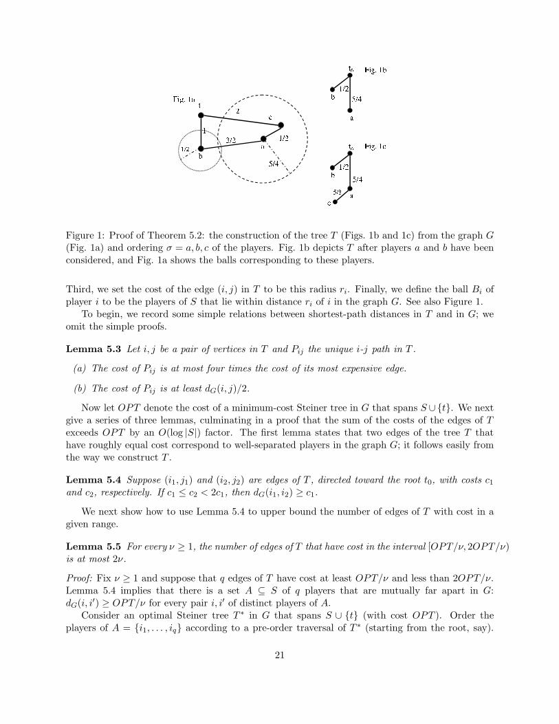
Figure 1: Proof of Theorem 5.2: the construction of the tree T (Figs. 1b and 1c) from the graph G(Fig. 1a) and ordering σ = a, b, c of the players. Fig. 1b depicts T after players a and b have beenconsidered, and Fig. 1a shows the balls corresponding to these players.

Third, we set the cost of the edge (i, j) in T to be this radius ri. Finally, we define the ball Bi ofplayer i to be the players of S that lie within distance ri of i in the graph G. See also Figure 1.

To begin, we record some simple relations between shortest-path distances in T and in G; weomit the simple proofs.

Lemma 5.3 Let i, j be a pair of vertices in T and Pij the unique i-j path in T .

(a) The cost of Pij is at most four times the cost of its most expensive edge.

(b) The cost of Pij is at least dG(i, j)/2.

Now let OPT denote the cost of a minimum-cost Steiner tree in G that spans S ∪t. We nextgive a series of three lemmas, culminating in a proof that the sum of the costs of the edges of Texceeds OPT by an O(log |S|) factor. The first lemma states that two edges of the tree T thathave roughly equal cost correspond to well-separated players in the graph G; it follows easily fromthe way we construct T .

Lemma 5.4 Suppose (i1, j1) and (i2, j2) are edges of T , directed toward the root t0, with costs c1

and c2, respectively. If c1 ≤ c2 < 2c1, then dG(i1, i2) ≥ c1.

We next show how to use Lemma 5.4 to upper bound the number of edges of T with cost in agiven range.

Lemma 5.5 For every ν ≥ 1, the number of edges of T that have cost in the interval [OPT/ν, 2OPT/ν)is at most 2ν.

Proof: Fix ν ≥ 1 and suppose that q edges of T have cost at least OPT/ν and less than 2OPT/ν.Lemma 5.4 implies that there is a set A ⊆ S of q players that are mutually far apart in G:dG(i, i′) ≥ OPT/ν for every pair i, i′ of distinct players of A.

Consider an optimal Steiner tree T ∗ in G that spans S ∪ t (with cost OPT ). Order theplayers of A = i1, . . . , iq according to a pre-order traversal of T ∗ (starting from the root, say).

21

As is well known, we can double every edge of T ∗ and decompose the resulting multigraph into acollection of paths that connect pairs of adjacent players (including i1 and iq). This proves that∑q

j=1 dG(ij , ij+1) ≤ 2OPT , where iq+1 refers to player i1. Thus dG(ij , ij+1) ≤ 2OPT/q for somej ∈ 1, 2, . . . , q. Since dG(i, i′) ≥ OPT/ν for every i, i′ ∈ A, q ≤ 2ν.

We now combine Lemma 5.5 with a grouping argument to upper bound the sum of the edgecosts in the tree T .

Lemma 5.6 The sum of the costs of the edges in T is at most (4 log2 |S| + 5) · OPT .

Proof: First, note that every edge cost in T is bounded above by the distance dG(i, t) in G betweenthe root t and some player i of S. Since every such distance is a lower bound on OPT , every edgeof T has cost at most OPT .

Next, let k = |S| and consider the edges with cost in the interval [2iOPT/k, 2i+1OPT/k) forsome i ∈ 0, 1, . . . , ⌊log2 k⌋. By Lemma 5.5, there are at most k/2i−1 edges in this group. Thesum of the edge costs in each of the ⌈log2 k⌉ groups is therefore at most 4OPT . Since T has k + 1vertices, it has k edges, and thus the total cost of the edges not in any of these groups — each ofwhich has cost less than OPT/k — is at most OPT . Summing over all of the edges proves thelemma.

Next, let χTsh(iℓ, Sℓ) denote the Shapley cost share of the ℓth player (in the given ordering σ) in

the fixed-tree multicast instance corresponding to the tree T and the set Sℓ of the first ℓ playersaccording to σ. Since fixed-tree multicast cost-sharing problems are submodular (Example 2.1),inequality (13) and Lemma 5.6 immediately give the following upper bound on the sum of theseShapley cost shares.

Lemma 5.7 Let iℓ denote the ℓth player and Sℓ the first ℓ players of S according to σ, respectively.Then

|S|∑

ℓ=1

χTsh(iℓ, Sℓ) ≤ (ln |S| + 1) · (4 log2 |S| + 5) · OPT.

Finally, we show that the JV cost share of a player in G is at most a constant factor timesits Shapley cost share in T . This is the step of the proof of Theorem 5.2 where we use specificproperties of the JV cost-sharing method (Proposition 5.1).

Lemma 5.8 Let iℓ denote the ℓth player and Sℓ the first ℓ players of S according to σ, respectively.For every ℓ ∈ 1, 2, . . . , |S|,

χJV (iℓ, Sℓ) ≤ 8 · χTsh(iℓ, Sℓ).

Proof: Fix ℓ ∈ 1, 2, . . . , |S| and let e1, e2, . . . , ep denote the sequence of edges in the iℓ-t0 path inT . Let cj denote the cost of edge ej. Let Aj ⊆ Sℓ denote the players of Sℓ whose path to t0 in Tcontains the edge ej . Let mj denote the number |Aj | of such players.

Our tree construction ensures that children of iℓ correspond only to players subsequent to iℓ inthe ordering σ, and no such players are in Sℓ. Thus A1 = iℓ, and of course A1 ⊆ · · · ⊆ Ap ⊆ Sℓ.First, observe that

χTsh(iℓ, Sℓ) =

p∑

j=1

cj

mj. (14)

22

Next, fix j ∈ 2, 3, . . . , p and consider a player i ∈ Aj distinct from iℓ. Since the edge ej separatesplayers i and iℓ from t0 in T , the most expensive edge on the iℓ-i path P in T has cost at mostcj−1. By Lemma 5.3(a), the path P has cost at most 4cj−1. By Lemma 5.3(b), the distancedG(iℓ, i) between the players in G is at most 8cj−1. By Proposition 5.1(c), the players iℓ and iare in a common connected component by the time 8cj−1 in the execution of Edmonds’s algorithmthat defines the JV cost share χJV (iℓ, Sℓ). Crucially, it follows that if player iℓ is active at a timesubsequent to 8cj−1 in this execution, then its weakly connected component at this time does notcontain the root t and contains at least the mj (active) players of Aj . Similarly, Lemma 5.3 andProposition 5.1(b) imply that player iℓ is inactive by the time 8cp.

Combining these observations with Proposition 5.1(a), we obtain

χJV (iℓ, Sℓ) ≤p

∑

j=1

∫ 8cj

8cj−1

dt

mj≤ 8

p∑

j=1

cj

mj, (15)

where we are interpreting c0 as 0. Comparing equality (14) and inequality (15) proves the lemma.

Theorem 5.2 now follows immediately from Lemma 5.7, Lemma 5.8, and Theorem 3.4.

5.3 Every Moulin Mechanism is Ω(log2k)-Approximate

This section proves that the JV mechanism is an optimal Moulin mechanism for Steiner tree cost-sharing problems, in the sense that every no-deficit mechanism for such problems is Ω(log2 k)-approximate, where k is the size of an efficient outcome. To motivate our proof of this result, webegin with an example showing that our analysis of the JV mechanism is tight up to constantfactors.

Example 5.9 We construct a Steiner tree instance in rounds by iteratively bisecting an edge ofcost 1 as follows. Initially we place the root t at one end of the edge and

√n players at the other

end of the edge. (Think of n as a large power of 4.) In the second round, we bisect the edge witha new vertex in the middle and add

√n further players co-located at this vertex. In round j, we

bisect the existing 2j−1 edge segments and, for each new node, we add√

n new co-located players.The construction concludes when there are n players, after Θ(log n) rounds.

Order the players in the same order in which they were added during the construction; breakties among players added in the same round arbitrarily. This defines n successive Steiner treeinstances. Consider the cost share of the most recently added player of one of these instances. TheJV cost-sharing method satisfies the following property: if a player is co-located with i − 1 otherplayers (all added earlier) and is distance c away from the nearest non-co-located player that wasadded in an earlier round, then its cost share in this instance is Ω(c/i). Because of this, the sum ofthe cost shares of players added in the jth round of the above construction is Ω(log n). Since thereare Ω(log n) rounds, the sum of all of these successive cost shares is Ω(log2 n). Since the minimum-cost Steiner tree of the full instance has cost 1 and the JV cost-sharing method is positive in thisinstance, Proposition 3.10 implies that the induced Moulin mechanism is Ω(log2 n)-approximate.

The main result of this section is a comparable lower bound for every O(1)-budget-balancedMoulin mechanism.

23

root t

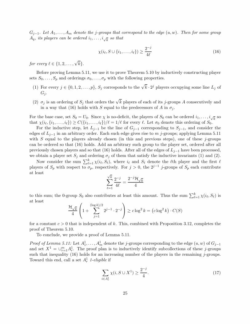
Figure 2: Network G2 in the proof of Theorem 5.10, with m = 3. All edges have length 1/4.

Theorem 5.10 There is a constant c > 0 such that, for every constant β ≥ 1, every β-budget-balanced Moulin mechanism for Steiner tree cost-sharing problems is no better than strongly (c log2 k)-approximate, where k is the number of players served in an optimal outcome.

Theorem 5.10 implies that Steiner tree cost-sharing problems are fundamentally more difficult forMoulin mechanisms than submodular cost-sharing problems (cf., Section 4).

We now outline the proof of Theorem 5.10. At the highest level, our goal is to exhibit a (large)network G such that every O(1)-budget-balanced Steiner tree Moulin mechanism behaves like theJV mechanism in Example 5.9 on some subnetwork of G.

Fix values for the parameters k and β, where k is a power of 4. Let m be an integer with

m ≥ 8β√

k · (2β)√

k. We construct a sequence of networks, culminating in G. The network G0

consists of a set V0 of two nodes connected by an edge of cost 1. One of these is the root t. Theplayer set U0 is

√k players that are co-located at the non-root node. For j > 0, we obtain the

network Gj from Gj−1 by replacing each edge (u,w) of Gj−1 with m internally disjoint two-hoppaths between u and w. See Figure 2. The cost of each of these 2m edges is half of the cost of theedge (u,w). Thus every edge in Gj has cost 2−j .

Let Vj denote the vertices of Gj that are not also present in Gj−1. We augment the universeby placing

√k new co-located players at each vertex of Vj; call each of these groups a j-group

and denote the union of them by Uj . The final network G is then Gp, where p = (log2 k)/2. LetV = V0 ∪ · · · ∪ Vp and U = U0 ∪ · · · ∪ Up denote the corresponding vertex and player sets. Let Cdenote the corresponding Steiner tree cost function.

A line in Gj is a subgraph defined inductively as follows. The only line in G0 is all of G0. Each

line Lj−1 of Gj−1 gives rise to a set of m2jlines in Gj , each obtained by replacing each edge of Lj−1

by one of the m two-hop paths to which it corresponds in Gj . Every line in the network Gj has 2j

vertices other than the root, 2j edges, and unit total cost. In Gp,√

k players inhabit each of the2p =

√k non-root vertices on a line.

Now fix an arbitrary cross-monotonic, β-budget balanced Steiner tree cost-sharing method χ.Our plan is to identify a line of Gp and an ordering of the players on this line such that χ behaveslike the JV cost-sharing method in Example 5.9. We construct this line iteratively via the followingkey technical lemma.

Lemma 5.11 Let S ⊆ U be a subset of players that lies on a line in Gp, includes at least oneplayer of U0, and includes at least one player each from a pair u,w of vertices that are adjacent in

24

Gj−1. Let A1, . . . , Am denote the j-groups that correspond to the edge (u,w). Then for some groupAq, its players can be ordered i1, . . . , i√k so that

χ(iℓ, S ∪ i1, . . . , iℓ) ≥2−j

4ℓ(16)

for every ℓ ∈ 1, 2, . . . ,√

k.

Before proving Lemma 5.11, we use it to prove Theorem 5.10 by inductively constructing playersets S0, . . . , Sp and orderings σ0, . . . , σp with the following properties.

(1) For every j ∈ 0, 1, 2, . . . , p, Sj corresponds to the√

k · 2j players occupying some line Lj ofGj .

(2) σj is an ordering of Sj that orders the√

k players of each of its j-groups A consecutively andin a way that (16) holds with S equal to the predecessors of A in σj .

For the base case, set S0 = U0. Since χ is no-deficit, the players of S0 can be ordered i1, . . . , i√k sothat χ(iℓ, i1, . . . , iℓ) ≥ C(i1, . . . , iℓ)/ℓ = 1/ℓ for every ℓ. Let σ0 denote this ordering of S0.

For the inductive step, let Lj−1 be the line of Gj−1 corresponding to Sj−1, and consider theedges of Lj−1 in an arbitrary order. Each such edge gives rise to m j-groups; applying Lemma 5.11with S equal to the players already chosen (in this and previous steps), one of these j-groupscan be ordered so that (16) holds. Add an arbitrary such group to the player set, ordered after allpreviously chosen players and so that (16) holds. After all of the edges of Lj−1 have been processed,we obtain a player set Sj and ordering σj of them that satisfy the inductive invariants (1) and (2).

Now consider the sum∑k

ℓ=1 χ(iℓ, Sℓ), where iℓ and Sℓ denote the ℓth player and the first ℓplayers of Sp with respect to σp, respectively. For j > 0, the 2j−1 j-groups of Sp each contributeat least √

k∑

ℓ=1

2−j

4ℓ=

2−jH√k

4

to this sum; the 0-group S0 also contributes at least this amount. Thus the sum∑k

ℓ=1 χ(iℓ, Sℓ) isat least

H√k

4

1 +

(log k)/2∑

j=1

2j−1 · 2−j

≥ c log2 k =(

c log2 k)

· C(S)

for a constant c > 0 that is independent of k. This, combined with Proposition 3.12, completes theproof of Theorem 5.10.

To conclude, we provide a proof of Lemma 5.11.

Proof of Lemma 5.11: Let A11, . . . , A

1m denote the j-groups corresponding to the edge (u,w) of Gj−1

and set X1 = ∪mr=1A

1r. The proof plan is to inductively identify subcollections of these j-groups

such that inequality (16) holds for an increasing number of the players in the remaining j-groups.Toward this end, call a set A1

r 1-eligible if

∑

i∈A1r

χ(i, S ∪ X1) ≥ 2−j

4. (17)

25

Every 1-eligible group contains a player i for which χ(i, S ∪ X1) ≥ 2−j/4√

k.Our key claim is that at least m/2β groups are 1-eligible. We prove this claim via an averaging

argument that relies on the β-budget-balance and cross-monotonicity of χ. Precisely, reindex the1-eligible groups A1

1, . . . , A1q and let Y 1 denote their union. An optimal Steiner tree spanning S∪Y 1

consists of a line through S and one group of Y 1, plus q − 1 “spokes” attaching the rest of thegroups to either u or w. Thus C(S ∪ Y 1) = 1 + (q − 1)2−j . Since χ is cross-monotonic andβ-budget-balanced, we have

∑

i∈S∪Y 1

χ(i, S ∪ X1) ≤∑

i∈S∪Y 1

χ(i, S ∪ Y 1) ≤ β(1 + (q − 1)2−j).

Since (17) fails for ineligible groups, and there at most m such groups,

∑

i∈X1\Y 1

χ(i, S ∪ X1) ≤ m2−j

4.

On the other hand, since C(S ∪ X1) = 1 + (m − 1)2−j and χ is no-deficit,

∑

i∈S∪X1

χ(i, S ∪ X1) ≥ 1 + (m − 1)2−j .

Combining these three inequalities and rearranging gives the constraint

q ≥ 3m

4β− 2j − 1

β≥ m

2β,

where the second inequality holds because m is sufficiently large.Now we iterate the process. In more detail, obtain A2

r from each 1-eligible group A1r by removing

a player i for which χ(i, S ∪ X1) ≥ 2−j/4√

k. (Such a player must exist by 1-eligibility.) Let X2

denote the union of these sets. Such a set A2r is 2-eligible if

∑

i∈A2r

χ(i, S ∪ X2) ≥ 2−j

4.

Every 2-eligible j-group contains a player i for which χ(i, S ∪ X2) ≥ 2−j/4(√

k − 1). Arguing asabove, at least a 1/2β fraction of the sets A2

r are 2-eligible.Iterating this procedure and reindexing the eligible groups after each iteration, we inductively

obtain a collection of disjoint sets Ah1 , . . . , Ah

qhfor each h ∈ 1, 2, . . . ,

√k with the following prop-

erties:

(1) qh ≥ m/(2β)h;

(2) for each r ∈ 1, . . . , qh, Ahr contains a player ihr such that χ(ihr , S ∪Xh) ≥ 2−j/4(

√k−h+1),

where Xh = ∪rAhr ;

(3) for each r ∈ 1, . . . , qh and h > 1, Ahr = Ah−1

r \ ih−1r .

Since m is sufficiently large, q√k ≥ 1. By properties (2) and (3) and cross-monotonicity of χ, the

group A11 that corresponds to A

√k

1 satisfies the requirements of the lemma.

26

6 Budget-Balance vs. Economic Efficiency Trade-Offs

No-deficit Moulin mechanisms are inefficient because of their overzealous removal of players thatcannot pay their cost share (cf., Examples 2.12 and 3.1). This suggests a possible trade-off betweenbudget-balance and economic efficiency: if we relax the requirement that the prices charged coverthe cost incurred, then a Moulin mechanism can employ smaller cost shares and reduce the worst-case efficiency loss from regrettable player deletions. This section extends the efficiency guaranteesof Section 3 to mechanisms that need not cover the incurred cost, and uses these extensions toquantify the trade-off between budget-balance and economic efficiency in Moulin mechanisms forsubmodular and Steiner tree cost-sharing problems. In particular, we show that relaxing budget-balance permits mechanisms with strictly better efficiency guarantees than those possible for no-deficit Moulin mechanisms.

Recall that a Moulin mechanism is (β, γ)-budget-balanced if the sum of the prices charged is atleast 1/γ and at most β times the incurred service cost. When γ > 1, Moulin mechanisms cansuffer efficiency loss from the unjustified service of players with low valuations. (See Example 6.5below.) For this reason, an efficiency guarantee for a (β, γ)-budget-balanced Moulin mechanismmust reference both the parameter γ and the summability of its underlying cost-sharing method.We provide such a guarantee next.

Theorem 6.1 Let C be a cost function defined on a universe U and χ a cross-monotonic, (β, γ)-budget-balanced, α-summable cost-sharing method for C. Let SM and S∗ denote the outcome chosenby M(χ) and an optimal outcome, respectively, for a valuation profile v. Then,

W (S∗) − W (SM ) ≤ (α(|S∗|) − 1 + β(γ − 1)) · C(S∗) + (γ − 1) · v(SM \ S∗).

Proof: Define an ordering σ on U and a potential function Φσ as in the proof of Theorem 3.4. Byfollowing the steps in that proof and using the (β, γ)-budget-balance of χ, we obtain

v(U \ SM ) + C(SM ) ≤ v(U \ SM ) + γ∑

i∈SM

χ(i, SM )

≤ v(U \ SM ) + γ · v(SM \ S∗) + γ∑

i∈SM∩S∗

χ(i, SM )

≤ Φσ(SM ∩ S∗) + (γ − 1) · v(SM \ S∗) + (γ − 1)∑

i∈SM∩S∗

χ(i, SM ∩ S∗)

≤ Φσ(S∗) + (γ − 1) · v(SM \ S∗) + (γ − 1)β · C(S∗)

≤ (α(|S∗|) + β(γ − 1)) · C(S∗) + v(U \ S∗) + (γ − 1) · v(SM \ S∗).

Rearranging terms proves the theorem.

Theorem 6.1 is tight in the following sense: for every choice of values for the parameters α(|S∗|),β, and γ, there is a cost-sharing problem and a Moulin mechanism with these parameter valuessuch that its welfare loss can be arbitrarily close to the upper bound in Theorem 6.1.

Like Theorem 3.4, the guarantee on additive welfare loss in Theorem 6.1 can be interpreted inseveral different ways. We mention only the cleanest such interpretation, in terms of minimizingthe social cost objective (2).

27

Corollary 6.2 Let C be a cost function defined on a universe U and χ a cross-monotonic, (β, γ)-budget-balanced, α-summable cost-sharing method for C. Then M(χ) is a (maxα(k)+β(γ−1), γ)-approximation algorithm for the social cost objective, where k is the size of an efficient outcome.

For example, for a submodular cost-sharing problem with n players, dividing the correspondingShapley cost shares by an

√Hn factor yields a (1,√Hn)-budget-balanced and

√Hn-summable cost-sharing method. Corollary 6.2 implies the following guarantee for the induced Moulin mechanism(the scaled Shapley mechanism).

Corollary 6.3 For every n-player submodular cost-sharing problem, the scaled Shapley mechanismis (1,

√Hn)-budget-balanced and a (2

√Hn−1)-approximation algorithm for the social cost objective.

The scaled JV mechanism is defined by dividing the JV cost shares by a Θ(log n) factor.

Corollary 6.4 For every n-player Steiner tree cost-sharing problem, the scaled JV mechanism is(1, O(log n))-budget-balanced and an O(log n)-approximation algorithm for the social cost objective.

The efficiency guarantees in Corollaries 6.3 and 6.4 are better than the best possible for no-deficitMoulin mechanisms (Section 4 and Theorem 5.10).

Corollaries 6.3 and 6.4 are optimal efficiency guarantees in the following sense. First, a simpleexample shows that a Moulin mechanism that is no better than (β, γ)-budget-balanced is no betterthan a γ-approximation algorithm for the social cost.

Example 6.5 Let χ be a cross-monotonic cost-sharing method for a cost function C defined on auniverse U , and suppose that χ is no better than (β, γ)-budget-balanced for C. By definition, thereis a subset S ⊆ U of players with

∑

i∈S χ(i, S) ≤ C(S)/γ. Give each player i ∈ S the valuationχ(i, S) and other players zero valuations. With this valuation profile, the Moulin mechanism M(χ)outputs a set containing all of the players of S, with social cost at least C(S). The optimal socialcost is at most that of the empty set, which is at most C(S)/γ.

Second, the lower bound proofs in Section 4 and of Theorem 5.10 extend easily to show that all(β, γ)-budget-balanced Moulin mechanisms for submodular and Steiner tree cost-sharing problemsare Ω((log k)/γ)- and Ω((log2 k)/γ)-approximation algorithms for the social cost, respectively. Thusno Moulin mechanism, no matter how poor its budget-balance, obtains an o(

√log k)-approximation

of the social cost for submodular problems or an o(log k)-approximation of the social cost for Steinertree problems.

7 Recent Work and Future Directions

We have developed an analysis framework for quantifying efficiency loss in Moulin mechanisms, andapplied this framework to identify the best efficiency guarantees achievable by such mechanisms insubmodular and Steiner tree cost-sharing problems, and to rigorously quantify the feasible trade-offs between efficiency and budget-balance. We conclude by discussing some of the very recentwork motivated by the conference version of this paper [41], and some possible directions for futureresearch.

The most obvious open problems suggested by our analysis framework are to establish matchingupper and lower bounds on the best-possible efficiency guarantees achievable by Moulin mechanisms

28

for additional classes of fundamental cost-sharing problems. Recent work has accomplished thisfor all of the classes of cost-sharing problems for which O(1)-budget-balanced Moulin mechanismsare known: facility location problems [42]; Steiner forest network design problems [9] and a prize-collecting generalization [19]; rent-or-buy network design problems [42]; and scheduling problems [8].

An important direction for further work is the design of non-Moulin cost-sharing mechanisms.Mehta, Roughgarden, and Sundararajan [33] recently extended Moulin mechanisms to a wider classthey call “acyclic mechanisms”, and prove that for several classes of cost-sharing problems, acyclicmechanisms can obtain approximate budget-balance and/or efficiency guarantees superior to thosepossible for Moulin mechanisms. Open problems include finding applications of acyclic mechanismsto new classes of cost-sharing problems, and generalizing acyclic mechanisms even further. On thenegative side, Dobzinski et al. [13] recently proved that the Ω(log n) approximate efficiency lowerbound of Section 4 is inescapable, even for mechanisms that are only truthful in expectation andapproximately budget-balanced.

A final direction is to completely characterize different classes of strategyproof cost-sharingmechanisms. Thus far, Moulin [35] characterized the groupstrategyproof (GSP) and 1-budget-balanced mechanisms (recall from Remark 2.11 that all Moulin mechanisms are GSP); Immorlica,Mahdian, and Mirrokni [23] partially characterized GSP mechanisms without any budget-balanceassumptions; and Juarez [26] very recently made progress toward characterizing “weakly GSP”cost-sharing mechanisms, a class that includes the acyclic mechanisms of [33]. Leveraging thesecharacterizations to obtain matching upper and lower bounds on the best-possible budget-balanceand efficiency guarantees achievable by the corresponding class of cost-sharing mechanisms is aworthy challenge for future research.

References

[1] N. Andelman, M. Feldman, and Y. Mansour. Strong price of anarchy. Games and EconomicBehavior, 2009. To appear.

[2] A. Archer, J. Feigenbaum, A. Krishnamurthy, R. Sami, and S. Shenker. Approximation andcollusion in multicast cost sharing. Games and Economic Behavior, 47(1):36–71, 2004.

[3] S. Arora and C. Lund. Hardness of approximations. In D. S. Hochbaum, editor, ApproximationAlgorithms for NP-Hard Problems, chapter 10, pages 399–446. PWS Publishing Company,1997.

[4] Y. Bachrach, E. Markakis, A. D. Procaccia, J. S. Rosenschein, and A. Saberi. Approximatingpower indices. In Proceedings of the 7th International Joint Conference on Autonomous Agentsand Multiagent Systems (AAMAS), pages 943–950, 2008.

[5] D. Bienstock, M. X. Goemans, D. Simchi-Levi, and D. P. Williamson. A note on the prize-collecting traveling salesman problem. Mathematical Programming, 59(3):413–420, 1993.

[6] Y. Bleischwitz and B. Monien. Fair cost-sharing methods for scheduling jobs on parallelmachines. In Proceedings of the 6th Italian Conference on Algorithms and Complexity (CIAC),volume 3998 of Lecture Notes in Computer Science, pages 175–186, 2006.

[7] A. Borodin and R. El-Yaniv. Online Computation and Competitive Analysis. CambridgeUniversity Press, 1998.

29

[8] J. Brenner and G. Schafer. Cost sharing methods for makespan and completion time schedul-ing. In Proceedings of the 24th International Symposium on Theoretical Aspects of ComputerScience (STACS), volume 4393 of Lecture Notes in Computer Science, pages 670–681, 2007.

[9] S. Chawla, T. Roughgarden, and M. Sundararajan. Optimal cost-sharing mechanisms fornetwork design. In Proceedings of the Second Annual International Workshop on Internetand Network Economics (WINE), volume 4286 of Lecture Notes in Computer Science, pages112–123, 2006.

[10] S. A. Cook. The complexity of theorem-proving procedures. In Proceedings of the 3rd AnnualACM Symposium on the Theory of Computing (STOC), pages 151–158, 1971.

[11] R. Deb and L. Razzolini. Auction-like mechanisms for pricing excludable public goods. Journalof Economic Theory, 88(2):340–368, 1999.

[12] N. R. Devanur, M. Mihail, and V. V. Vazirani. Strategyproof cost-sharing mechanisms for setcover and facility location games. Decision Support Systems, 39(1):11–22, 2005.

[13] S. Dobzinski, A. Mehta, T. Roughgarden, and M. Sundararajan. Is Shapley cost-sharingoptimal? In Proceedings of the First International Symposium on Algorithmic Game Theory(SAGT), volume 4997 of Lecture Notes in Computer Science, pages 327–336, 2008.

[14] J. Edmonds. Optimum branchings. Journal of Research of the National Bureau of Standards,Series B, 71(4):233–240, 1967.

[15] J. Feigenbaum, A. Krishnamurthy, R. Sami, and S. Shenker. Hardness results for multicastcost sharing. Theoretical Computer Science, 304(1-3):215–236, 2003.

[16] J. Feigenbaum, C. Papadimitriou, and S. Shenker. Sharing the cost of multicast transmissions.Journal of Computer and System Sciences, 63(1):21–41, 2001.

[17] J. Feigenbaum and S. J. Shenker. Distributed algorithmic mechanism design: Recent resultsand future directions. In Proceedings of the 6th International Workshop on Discrete Algorithmsand Methods for Mobile Computing and Communications, pages 1–13, 2002.

[18] J. Green, E. Kohlberg, and J. J. Laffont. Partial equilibrium approach to the free rider problem.Journal of Public Economics, 6(4):375–394, 1976.

[19] A. Gupta, J. Konemann, S. Leonardi, R. Ravi, and G. Schafer. An efficient cost-sharingmechanism for the prize-collecting Steiner forest problem. In Proceedings of the 18th AnnualACM-SIAM Symposium on Discrete Algorithms (SODA), pages 1153–1162, 2007.

[20] A. Gupta, A. Srinivasan, and E. Tardos. Cost-sharing mechanisms for network design. Algo-rithmica, 50(1):98–119, 2008.

[21] S. Hart and A. Mas-Colell. Potential, value, and consistency. Econometrica, 57(3):589–614,1989.

[22] J. D. Hartline. Optimization in the Private Value Model: Competitive Analysis Applied toAuction Design. PhD thesis, University of Washington, 2003.

30

[23] N. Immorlica, M. Mahdian, and V. S. Mirrokni. Limitations of cross-monotonic cost-sharingschemes. ACM Transactions on Algorithms, 4, 2008. Article 24.

[24] K. Jain and V. Vazirani. Applications of approximation algorithms to cooperative games. InProceedings of the 33rd Annual ACM Symposium on the Theory of Computing (STOC), pages364–372, 2001.

[25] K. Jain and V. Vazirani. Equitable cost allocations via primal-dual-type algorithms. SIAMJournal on Computing, 38(1):241–256, 2008.

[26] R. Juarez. Group strategyproof cost sharing: the role of indifferences. Working paper, 2007.

[27] K. Kent and D. Skorin-Kapov. Population monotonic cost allocation on MST’s. In OperationalResearch Proceedings KOI, pages 43–48, 1996.

[28] J. Kleinberg and E. Tardos. Approximation algorithms for classification problems with pairwiserelationships: metric labeling and markov random fields. Journal of the ACM, 49(5):616–639,2002.

[29] J. Konemann, S. Leonardi, G. Schafer, and S. van Zwam. A group-strategyproof mechanismfor the Steiner forest game. SIAM Journal on Computing, 37(5):1319–1341, 2008.

[30] S. Leonardi and G. Schafer. Cross-monotonic cost-sharing methods for connected facilitylocation. Theoretical Computer Science, 326(1-3):431–442, 2004.

[31] F. Maniquet and Y. Sprumont. Fair production and allocation of an excludable nonrival good.Econometrica, 72(2):627–640, 2004.

[32] A. Mas-Colell, M. D. Whinston, and J. R. Green. Microeconomic Theory. Oxford UniversityPress, 1995.

[33] A. Mehta, T. Roughgarden, and M. Sundararajan. Beyond Moulin mechanisms. Games andEconomic Behavior, 2009. To appear.

[34] D. Monderer and L. S. Shapley. Potential games. Games and Economic Behavior, 14(1):124–143, 1996.

[35] H. Moulin. Incremental cost sharing: Characterization by coalition strategy-proofness. SocialChoice and Welfare, 16(2):279–320, 1999.

[36] H. Moulin and S. Shenker. Strategyproof sharing of submodular costs: Budget balance versusefficiency. Economic Theory, 18(3):511–533, 2001.

[37] S. Muthukrishnan. Data streams: Algorithms and applications. Foundations and Trends inTheoretical Computer Science, 1(2):117–236, 2005.

[38] M. J. Osborne and A. Rubinstein. A Course in Game Theory. MIT Press, 1994.

[39] M. Pal and E. Tardos. Group strategyproof mechanisms via primal-dual algorithms. InProceedings of the 44th Annual Symposium on Foundations of Computer Science (FOCS),pages 584–593, 2003.

31

[40] K. Roberts. The characterization of implementable choice rules. In J. J. Laffont, editor,Aggregation and Revelation of Preferences. North-Holland, 1979.

[41] T. Roughgarden and M. Sundararajan. New trade-offs in cost-sharing mechanisms. In Pro-ceedings of the 38th Annual ACM Symposium on the Theory of Computing (STOC), pages79–88, 2006.

[42] T. Roughgarden and M. Sundararajan. Optimal efficiency guarantees for network designmechanisms. In Proceedings of the 12th Conference on Integer Programming and CombinatorialOptimization (IPCO), volume 4513 of Lecture Notes in Computer Science, pages 469–483, 2007.

[43] W. Vickrey. Counterspeculation, auctions, and competitive sealed tenders. Journal of Finance,16(1):8–37, 1961.

32