quantifying risk of ground impact fatalities for small
TRANSCRIPT

Aalborg Universitet
Quantifying Risk of Ground Impact Fatalities for Small Unmanned Aircraft
La Cour-Harbo, Anders
Published in:Journal of Intelligent and Robotic Systems
DOI (link to publication from Publisher):10.1007/s10846-018-0853-1
Creative Commons LicenseCC BY 4.0
Publication date:2019
Document VersionPublisher's PDF, also known as Version of record
Link to publication from Aalborg University
Citation for published version (APA):La Cour-Harbo, A. (2019). Quantifying Risk of Ground Impact Fatalities for Small Unmanned Aircraft. Journal ofIntelligent and Robotic Systems, 93(1-2), 367-384. https://doi.org/10.1007/s10846-018-0853-1
General rightsCopyright and moral rights for the publications made accessible in the public portal are retained by the authors and/or other copyright ownersand it is a condition of accessing publications that users recognise and abide by the legal requirements associated with these rights.
? Users may download and print one copy of any publication from the public portal for the purpose of private study or research. ? You may not further distribute the material or use it for any profit-making activity or commercial gain ? You may freely distribute the URL identifying the publication in the public portal ?
Take down policyIf you believe that this document breaches copyright please contact us at [email protected] providing details, and we will remove access tothe work immediately and investigate your claim.
Downloaded from vbn.aau.dk on: December 13, 2021

Journal of Intelligent & Robotic Systemshttps://doi.org/10.1007/s10846-018-0853-1
Quantifying Risk of Ground Impact Fatalities for Small UnmannedAircraft
Anders la Cour-Harbo1
Received: 30 September 2017 / Accepted: 17 April 2018© The Author(s) 2018
AbstractOne of the major challenges of conducting operations of unmanned aircraft, especially operations beyond visual line-of-sight (BVLOS), is to make a realistic and sufficiently detailed risk assessment. An important part of such an assessment isto identify the risk of fatalities, preferably in a quantitative way since this allows for comparison with manned aviation todetermine whether an equivalent level of safety is achievable. This work presents a method for quantifying the probability offatalities resulting from an uncontrolled descent of an unmanned aircraft conducting a BVLOS flight. The method is basedon a standard stochastic model, and employs a parameterized high fidelity ground impact distribution model that accountsfor both aircraft specifications, parameter uncertainties, and wind. The method also samples the flight path to create analmost continuous quantification of the risk as a function of mission flight time. The methodology is exemplified with a 180km flight in Danish airspace with a Penguin C aircraft.
Keywords Unmanned aircraft · Aviation safety · Stochastic modeling · Ground impact · Probability of fatality
1 Introduction
1.1 Background
As drones are becoming ubiquitous in the airspace andas more applications of drones are focused on longerflights the need for reliable, detailed, and quantitative riskassessment methods is growing. While there are severalmethods available (borrowing from manned aviation) forqualitatively identifying and categorizing hazards andmitigating risks there is comparatively little methodologyavailable for actually determining the probability of fatalityfor a particular drone operation in particular methodsthat lend themselves to reverse engineering to allow forpinpointing how a given flight scenario could be altered toreduce the risk. This is in large part due to the seeminglyendless list of variables that enters such a method were it tobe completely comprehensive.
This particular work is prompted by a decision bythe Danish Transport Construction and Housing Authority
� Anders la [email protected]
1 Aalborg University, Fredrik Bajers Vej 7C, 9220 Aalborg East,Denmark
in 2016 to conducts a number of trial BVLOS flightoperations in Danish airspace with the expressed intent ofusing these to pave the way for routine BVLOS operationsby companies and other non-state actors. At that timeno permissions had been granted for BVLOS flight inDenmark except for flights in Greenland and individualflights confined to specific routes and dates. The trial flightswould be based on thorough analyzes of the risks, andthe idea was that subsequent flights would be conductedroutinely using the same risk assessment methodology.
This work presents the developed methodology. It isbased in part on a previous publication [21] applying themethodology to a power line inspection flight done bythe Danish company Heliscope. The present work expandsand details the methodology, and the example flight has adifferent and somewhat longer flight path as well as a moreprofessional drone platform.
1.2 PreviousWork
There are numerous works on how to conceptually approachthe challenge of determining the risk of an unmannedaircraft flight. Much is borrowed from the world of mannedaviation that has been conducting risk management fordecades. A number of examples of risk assessments andquantifications for unmanned aircraft include the following.

J Intell Robot Syst
In [4] a study for ground impact fatalities resultingfrom power failure and subsequent uncontrolled glide ispresented. A study on the impact area for a generaluncontrolled descent, including a buffer zone, is presentedin [17]. A method for automatically finding a proper landingarea for an aircraft in emergency descent is shown in[33, 34], and the ability of a fixed wing aircraft to glideto a designated emergency landing area is presented in[11]. In [3] a method for determining a no-thrust flighttrajectory to reach a particular landing spot is presented.The barrier bow tie model also used in manned aviationrisk assessment is presented in [8]. A study of trajectorymodels for explosive debris [29] attempts to determine theimpact point based on initial conditions. [10] addressesthe lack of an accepted framework and provides someguidelines for how to apply existing models to manage therisk. In [9] a comprehensive description of how to managethe risk of unmanned aircraft operations, including ’thesystematic application of management policies, proceduresand practices to the activities of communicating, consulting,establishing the context, and assessing, evaluating, treating,monitoring and reviewing risk.’ This work also presents aseries of quantification of existing risks for various typesof aviation. Metrics for safety, including hazard metricsand risks metrics are presented in [22], in [14] a softwaresafety case is developed, and in [13] a generic safety caseis presented based on experience with NASA unmannedaircraft missions. The uncontrolled descent of unmannedaircraft into populated areas have been the subject in anumber of publications. This includes [18] that investigatelarger aircraft through an equivalent level of safety analysis.[35] specifically looks at distribution of possible impactpositions based on simulation, and [7] uses the standardstatistical setup (which is also used in this work) andapplies a normal distribution approach using aircraft glideparameters to model the impact position.
1.3 Current Work
The aim in this work is to go beyond a qualitative approachthat merely provides a framework for risk assessment,and instead apply a quantitative approach to determineas accurately as possible, the level of safety for a givenflight operation using the metric ’fatalities per flight hour’,similar to what is used in manned aviation. The modelingof the probability of fatalities (POF) is done with astochastic approach similar to many of the previous workslisted above. However, the determination of the individualprobabilities in the model is done using georeferencedprobability density functions with high fidelity and (almost)continuously along the flight path to provide not just asingle probability for the entire flight, but indeed a fatalityrate along the flight path itself. This in turn allows for
easy identification of what parameters adversely affect theflight, with the possibility for reconfiguring the flight pathto reduce the risk of fatalities.
2Methods
The basic approach used in this work is similar to numerousprevious works, namely a stochastic model that joinsprobabilities in the causal chain from drone malfunction toa potential fatality. The specific design of this stochasticmodel varies from work to work. As described in Section 2.1below, we use a fairly simple setup, where the focus ison the probabilities related to the ground impact. Themodel is used for four different types of flight terminatingevents, all described in Section 2.2, each with their ownhigh resolution ground impact probability density function,see Sections 2.2.1 to 2.2.4, including the effect of wind,see Section 2.3, and associated event probability, seeSection 2.4. Rather than a priori assuming an averagepopulation density for the entire flight (as seen in manyprevious works), we employ high resolution populationdensity maps generated to fit the spatial extend of each eventtype, see Section 2.5. We then use the stochastic model ona (sufficiently densely) sampled flight path to determinethe probability of impacting a person as a function of theflight path. Finally, mapping from person impact to POF(probability of fatality) is applied based on work in the fieldof forensic science, see Section 2.7.
The POF for the entire flight is determine by summingover the flight path relative to the flight time betweeneach sample in the sampled flight path. This is doneseparately for the different types of flight terminating eventsto accommodate the varying lethality parameters associatedwith the manner in which the aircraft descents in each of theevent scenarios. The is described in more detail along withthe results in Section 3.
2.1 Overall Modeling Approach
For computing the probability of fatalities during the flightwe will use this formulation similar to what is used inseveral of the previous works listed in Section 1.2.
pfatality = pevent · pimpact person · pfatal impact , (1)
where pevent is the probability per time of a given event(of which we will use four), pimpact person is the conditionalprobability that given an occurrence of one of the eventsthat a person will be impacted as a result, and pfatal impact isthe conditional probability, given one or more persons areimpacted as a result of one of the events that this personsuffers a fatal injury. The primary focus in this work ison the probability that a descending aircraft will impact a
J Intell Robot Syst
person. We also briefly treat the probability of fatalities asa result of impact. The probability for each event occurringduring flight is measured in events per flight hour and willbe assumed known, since this probability is not the focus ofthis work. Determining such probabilities is no simple task,and in Section 2.4 is a brief discussion of the numbers usedfor exemplifying this work in Section 3.
For each type of event the probability of impactingpersons on the ground is determined in 4 steps:
1. Based on a model of a given event type a probabilitydensity function (PDF) is computed that determines theprobability of ground impact relative to the positionwhere the event happens.
2. This PDF is subjected to probabilistic wind, resulting ina new, often bigger, two-dimensional PDF, which canbe interpreted as a georeferenced probabilistic impactmap.
3. This map is correlated with a population density map ofsufficient resolution for the same geographical area.
4. The resulting map is integrated over the entire area andthe result is modified to account for various factorspertaining to each event type.
This gives a probability for a given event to result in animpact of a person on the ground relative to the eventposition. As a consequence this impact probability dependson the type of the event, aircraft parameters, wind, and flightpath of the aircraft. In the following sections the above stepsare discussed in more detail. But first the different typesof descents are listed in Section 2.2, and presented in moredetail in Sections 2.2.1 through 2.2.4.
2.2 Descent Event Types
We consider four rather different types of uncontrolleddescents of an unmanned aircraft. Each is a result ofvarying types of malfunction, and each has it own model (asindicated in step 1 above). We only consider events wherethe operator has no control authority and the aircraft descentpath therefore is governed mainly by aerodynamics or theautopilot. In either case the aircraft is not expected to returnhome nor to head for any designated safe impact zone.
1. Ballistic descent This is a situation where the aircrafthas lost most of its lift, for instance by a wing breakingoff or a motor physically separating from the aircraft.The aircraft will then enter a (close to) ballistic descentgoverned solely by the aerodynamics of the crippledaircraft.
2. Uncontrolled glide For a fixed wing aircraft thisis loss of thrust as well as loss of power for theflight control surfaces. For a helicopter type aircraftthis event could be loss of thrust on the main rotor
with an autopiloted autorotation descent. In any casethe airframe is structurally intact and the aircraft isassumed to enter a descent path governed by the glideratio/autorotation descent angle as well as wind. For afixed wing the deflection surfaces are assumed to be ina close to neutral position such as to give a straight orperhaps slightly curved glide.
3. Parachute descent This is a descent with a fullydeployed parachute. It is assumed that the deploymentis a result of a malfunction detection, and thus thatmotor(s) are turned off giving a descent path basedsolely on the aerodynamic properties of the parachute.
4. Flyaway This is complete loss of operator controlauthority of the aircraft while the autopilot continuousto operate in a mode that maintains the stability of theflight. The motion of the aircraft is controlled by theautopilot, and it may fly to its maximum range in anydirection, including vertically up.
One can envision additional failure scenarios such as aspin due to a faulty actuator, loss of a vital sensor thatdeprives the aircraft of any useful navigation, and so on.We assume that each of the four above listed events willhappen with a probability independent of where the aircraftis along the flight path. The impact point on the ground ofa descending aircraft is determined by the descent modelsrelative to the event point. The event point is defined asthe spatial location of the aircraft at the time it suffers amalfunction that gives raise to one of the above scenarios.Depending on the context the event point may refer to theprojection of the point onto the ground (i.e. zero AGL). Theground impact point position is modeled with a number ofuncertainties that reasonably may affect the descent, andthese are described below in more detail.
2.2.1 Ballistic Descent
The ballistic descent is modeled as described in [19]. Themodel has a second order dependence on speed and acts solelyunder influence of gravity and drag. The flight velocityprior to the event is based on the georeferenced flight path.The model for the ballistic descent is a multiple stage for-mulation that includes altitude, mass, drag coefficient, andfrontal area. The descent path is roughly a second orderpolynomial modified to account for the aerodynamic prop-erties of the aircraft. It also has probabilistic assumptions onthe horizontal and vertical initial speeds as well as on thedrag coefficient. The output of this model is a 1D PDF withthe probability of the aircraft impacting the ground a givendistance away from the event point and along a line coincid-ing with the traveling compass direction of the aircraft. Themodel is much too comprehensive to be reiterated here, sodo see the reference for further details.

J Intell Robot Syst
2.2.2 Uncontrolled Glide
The uncontrolled glide assumes the aircraft is descending asa glider. The aircraft is without thrust and in an aerodynamicequilibrium configuration with actuators in neutral or closeto neutral positions (that is, no banking with ailerons and noturning with the rudder). The horizontally traveled distanceper vertically descended distance is called the glide ratio γ ,and in this work is given as a normally distributed variablewith mean equal to the estimated glide ratio and a varianceto accommodate for variations in elevator deflection angleand variation in drag due to possible modifications of theaircraft to accommodate missions sensors. The horizontaldistance x traveled (in the wind frame) in an uncontrolledglide from altitude y is simply x(y) = γy and the droptime is tdrop(y) = x(y)/vg, where vg is the horizontal glidespeed. To get the ground impact PDF the wind variations asdescribed in Section 2.3 are applied.
2.2.3 Parachute Descent
Descent with a parachute is essentially a vertical drop in thewind frame. We assume that the parachute is deployed incase of a detected emergency situation with a short delay ofd seconds, and that the parachute once triggered will deployinstantaneously and reduce the horizontal velocity to zeroinstantly (in the wind frame). While this obviously in not thecase in real life the distance traveled during the deploymentand deceleration phase is negligible in relation to the impactarea for a parachuted descent. Assuming a standard secondorder drag model. The drop time from altitude y is
tdrop = y
vdrop= y
√ApCd,p
2mg, (2)
where m is mass, g is gravitational constant, Ap is parachutearea, and Cd,p is the parachute drag coefficient. In thiswork the latter is a probabilistic value. Note that if the dropspeed vdrop for a given parachute configuration is known theformula is very simple.
As with the uncontrolled glide the ground impactprobability density function (PDF) is achieved by applyingthe wind variations as described in Section 2.3 plusoffsetting the result according to the flight direction anddeployment delay.
2.2.4 Flyaway
A flyaway event will potentially take the aircraft to the limitof its range, which dependents largely on the fuel left andon the wind speed and direction. The model for a flyaway isin this work composed of two contributions.
First, the probability of ground impact is assumed todecreases linearly with distance from the event point,reaching zero at the maximum range. The simplicity ofthis model is primarily due to lack of knowledge of how aflyaway will progress. On the one hand if a flyaway mostoften will continue until there is no fuel left the probabilityof ground impact should be relatively higher close to thecircumference of the flight range circle. On the other handif the flyaway is not in a straight line, but rather more withrandom movements, and the ground impact point thereforecan be assumed to be equally likely at any distance fromthe event point, the probability should decrease with thesquare of the distance. As a compromise a linear relation ischosen. This probability is then modified according to thewind speed and direction. Mathematically, this is modeled as
f (p) = max
[0, Rmax − ‖p‖︸ ︷︷ ︸
linear decrease
+ cos(
arctanpN
pE+ θ
)‖p‖vc︸ ︷︷ ︸
modification according to wind
],
(3)
where θ is the wind average direction, Rmax is the maximumflight range given the available fuel, vc is the aircraft cruiseairspeed, and p = (pN, pE) is a north-east position relativeto the event point.
Second, a probability is added that the aircraft willascend more or less vertically, either as ’helicopter climb’or spiraling up with a fixed wing. This causes the groundimpact point to be close to the event point, and this partis modeled as a normal distribution for distance from theevent point with mean 0 and standard deviation σva (verticalascend) from the event point, and uniformly in direction.That is, the impact PDF becomes
g(p) = 1
2πσ 2va
exp
(−‖p‖2
2σ 2va
). (4)
The two scenarios as linearly combined with a relation factorβ, such that β = 0.5 makes each contributor with equalprobability. The resulting ground impact PDF becomes
Pflyaway(p) = (1 − β)f (p)∫∫ ∞
−∞ f (p)+ βg(p) . (5)
An example of the resulting 2D PDF is shown in Fig. 1.
2.3Wind
The influence of wind is significant for all four eventtypes. Ballistic descent, uncontrolled glide, and parachutedescent are all modeled directly in the wind frame, whilethe flyaway event is not directly assumed to be in the windframe, but the wind speed does in Eq. 3 affect the abilityof the aircraft to fly distances in certain directions. Sincethe knowledge about the wind for a given flight will vary

J Intell Robot Syst
-200
-100
0
100
200
300
Rela
tive n
orth
[km
]
-200 -100 0 100 200 300
Relative distance east [km]
10-7
10-6
10-5
10-4
Probability
Fig. 1 An example of a flyaway ground impact PDF. The upper graphshows the 2D PDF in log scale color and georeferenced relative tothe event location. The lower graph shows the maximum value alongthe north axis, also in log scale. Wind is heading 0.43 rad (circa east-north-east) at 5 m/s. The aircraft and parameters used are described inSection 3.1
somewhat depending on the circumstances we propose touse one of three wind models:
1. Direction and speed modeled with normal distributions.2. Direction unknown (modeled uniformly), speed mod-
eled with normal distribution.3. Direction and speed based on historic data.
The first option is useful for missions in a particulargeographical area where some wind statistics is available,and for computation just prior to a flight where the actualwind might be available. The second options is useful formore generic scenarios where the geographical locations isyet to be determined. The third option applies to scenariosthat take place at a known location at a known time, andwhere historic data for a the given time period (say aparticular week or month) is available.
The models for the ballistic descent, uncontrolled glide,and parachute descent all provide a series of drop times (thetime it takes the aircraft to reach the ground from the givenflight altitude) resulting from the probabilistic nature of the
models. For all three models the offset caused by the windis dependent solely on these drop times, since all other aero-dynamic properties are already accounted for in the models.
One way to practically compute the effect of the windis as follows. The range of possible drop times is sampledas {tk}k=0,...,n and for each drop time tk a sampledgeoreferenced PDF is generated as a matrix Mk representingthe probability of the aircraft doing a purely vertical dropin the wind frame to impact the ground at the geolocationrepresented by each entry in the matrix. The ground gridof the PDF (sampling density) should match the event typeand the population density matrix that appears later in thecomputation (see Section 2.5). The drop times comes fromthe individual models with a set of probabilities {pk}k=0,...,n
that gives the probability of each drop time. Thus, togenerate the wind effect on the individual model, we simplysum up the PDF matrices as
M =n∑
k=0
pkMk , (6)
while keeping score of the georeference of each matrixsuch that the resulting matrix M is also georeferenced. Thisapproach is particularly useful for flights where the samedrop times occurs often, since the Mk matrices need not berecalculated as long as the drop times are within the samerange.
To demonstrate how the wind effect is in practice appliedto a descent an example using the parachute descent is givenin Fig. 2. The procedure of applying wind to an uncontrolledglide and a ballistic descent is essentially the same.
2.4 Probability of Events
The events that render the aircraft uncontrollable and even-tually lead to a uncontrolled descent each has a probabilityattached to them. These probabilities are difficult to estimateand difficult to measure (as that would require many flighthours on precisely the same setup). For the computations inthis work we simply assume given values that per aviationtradition are measured in ’per flight hour’. The probabili-ties used here are estimates based on the works of others (seebelow) as well as the experience of persons at the insti-tutions listed in Acknowledgements. The event probabilityappears in the probability computation in Eq. 1 as a scalar.As a consequence the effect of changing the event probabil-ity is simply a scaling of the resulting probability.
The probability of a flight terminating malfunction onan unmanned aircraft has been studied by a number ofgroups. A reliability assessment of an Ultra Stick 120 ismade in [15] and [16] using failure mode effect and analysis(FMEA), with particular attention to the control surfacesand servos. No specific probabilities for an uncontrolled

J Intell Robot Syst
0.8 0.9 1 1.1 1.2 1.3 1.4 1.5
Drag coefficient
0.4
0.6
0.8
1
1.2
1.4
1.6
1.8
2
Pro
ba
bility
13
14
15
16
17
18
19
20
Dro
p t
ime
[s]
Distribution of Cd,p
Drop time tdrop
Graphed to the right
Drop time: 13.7 s
0
20
40
60
80
100
120
Re
lative
dis
tan
ce
no
rth
[m
]
Drop time: 17.0 s
Drop time: 19.8 s
50 100 150 200
Relative distance east [m]
0
20
40
60
80
100
120
Re
lative
dis
tan
ce
no
rth
[m
]
Combined
50 100 150 200
Relative distance east [m]
Fig. 2 Example of wind affecting a parachute descent: The graph onthe left shows in black the normal distribution N(μ = 1.14, σ 2 = 0.2)
of Cd,p, sampled 40 times from −2 to +2 standard deviations, and inblue the drop times associated with the same 40 Cd,p sample valuesfrom an altitude of 80 m with a parachute area of 12.5 m2 and air-craft mass of 16 kg. On the right is shown the wind PDF for three of
the drop times (marked in red on the blue graph on the left), usingwind direction distributed as N(0.44, 0.17) (equal to compass heading65◦ and standard deviation of 10◦) and speed as N(7, 2). The fourthgraph shows a linear combination as given by Eq. 6, and this wouldbe the non-offset (see Section 2.2.3 on parachute descent) georefer-enced ground impact PDF for a parachute descent relative to the eventposition at (0, 0)
descent are provided, but are considered to be high. In[24] probabilities related to military unmanned aircraft arereported, and the probability of a flight terminating eventis in the order of 10−4 – 10−2 per flight hour, with theprobability for smaller aircraft being somewhat higher thatfor the larger aircraft. A group of students showed in[26] using FMEA based on component failure rates thattheir Ultra Stick 120 has on average 2.17 catastrophic(flight terminating) failures per 100 flight hours. The typesof failures considered relate to the ballistic descent anduncontrolled glide in the present work. In [27] the samegroup showed how a dedicated reconstruction of the aircraftbased on a fault tree analysis could theoretically reducethe failure rate by a factor 20, and they were able toimplement changes to the physical aircraft to achieve acatastrophic failure rate of 0.76 per 100 flight hours.Actuators and control surfaces are investigated in [30] and[31] where the probability of having an uncontrollableaircraft is modeled using a servo fault detection algorithm.In [23] a method for estimating mechanical failure ratesof small unmanned aircraft is presented, and an exampleis provided based on the 25 kg SPAARO aircraft. Thisexample explicitly lists the used probabilities for failures ofservos and deflection surfaces as well as failures of engineand battery. These probabilities were provided by twoexperienced RC pilots. In addition probabilities of failurefor a wing bolt and main spar are theoretically derived. Theresulting failure rate for the aircraft (covering the ballistic
and uncontrolled glide events) is 0.19 failures per flighthour. With suggested improvements for the engine, wingbolt, servos, and redundant control surfaces the failure canbe reduced to 2.8 failure per 100 flight hours (equivalentto 36 hours between failures). Note that this includes non-catastrophic failures, where the aircraft may be able toreturn home.
2.5 People Density
Density of people on the ground is the main factor in theprobability of impacting a person in the event of a crash,and for BVLOS flight operations that stretches over longerdistances variation in people density can be significantduring the flight. The example flight presented in Section 3is specifically chosen to include this feature. As the impactareas for each event change over the course of the flight aswell as in between flight as a result of changes in altitude, windconditions, flight speeds etc. it is important to represent theactual people density with a reasonably fine resolution. Forthis reason it is insufficient to assume a fixed people density,even for smaller geographical areas, and if such assumptionis made the resulting POF may be misleading and changesin the flight planning that might actually have an impact onthe fatality rate may go unnoticed.
The impact area for different types of descents varieshugely, i.e. a ballistic descent is typically close to the eventposition, whereas a flyaway can result in a descent hundreds

J Intell Robot Syst
of kilometers from the event position. Consequently, forsome events the resolution of the people density map mustbe fairly high to give accurate estimates of the person impactprobability, while for other events the resolution can bemore coarse and still give accurate results.
A list of geographical coordinates of all addresses inDenmark is publicly available and this has been used togenerate people density maps with varying resolution tofit the different types of descents. While a fine grainedresolution will of course work for any type of eventthe computation time grows significantly, so maps aregenerated that suits the spatial extend of the impact area foreach type of event. In Fig. 3 are shown three examples ofsuch maps.
While these maps do show where people live theyobviously do not show where people actually are. Asthis information is evidently very difficult to obtain wewill make the assumptions that people are, with someprobability, in the vicinity of their home, and with someprobability are outside exposed to a small unmanned aircraftpotentially descending. Inspired by [12] an appropriateprobability of people being exposed is around 30%. Thisis also referred to as the shelter factor. We will alsoassume that the number of people associated with eachaddress is equal to the average number of people in aDanish household. This number is 5.75 million peopledivided by 2.65 million households, equal to 2.17 peopleper household. The number of addresses is 3.3 million assome addresses are not households, but rather businessesand industry. The density map used in this work is notadjusted to account for this.
2.6 Probability of Impact Persons
For a given event type we now have a ground impactprobability density function (PDF) measured in metersrelative to (0, 0). By offsetting this PDF relative to thecoordinates of the event point we obtain a georeferenced
impact map in WGS84 coordinates (latitude and longitude).This PDF matrix is then entry-wise multiplied with thepopulation density map (appropriately sampled matrix D)for the same area and the result is a map of the probabilityof impacting a 1 m2 large person, since our populationdensity is measured in people per m2. We assume that aperson takes up a particular area Aperson that depends onthe expected impact angle, and this value is multiplied ontothe result. Additionally, it is multiplied with the shelterfactor S, which accounts for the probability that a personis sheltered by being indoors, under a tree, in a car etc.In this work we assume a fairly high probability of beingsheltered (typically indoors), since the population densitymap is based on addresses where people live. This will thenprovide the probability pimpact person of impacting a person(see Eq. 1 above) given a particular event at the given eventpoint. The computation can be formulated as
pimpact person = S · Aperson ·∑
latitudelongitude
(PDF ◦ D) , (7)
where ◦ is the Hadamard product and · is the scalar product.
2.7 Probability of Fatality When Impacted
When a drone impacts a human there is a probability thatthe impact will inflect injuries that will result in a fatality.Determining this probability for a given person and a givendrone is not simple, partly because of the many differentways the impact can occur, and partly because the easilydetermined parameters, such a speed and mass, do not havea simple correlation to injury severity, because the humanbody reacts differently depending on the impacted bodypart, and the fact that injuries primarily relate to how fastand where the kinetic energy is dissipated in the body, notthe kinetic energy of the impacting object itself. For a reviewof literature on drone-like human injuries, see [20] and [2].A number of reasonably accurate and empirically verified
Fig. 3 From left to right people density maps with resolutions of 1 km,100 m, and 25 m. The color scale is the same and goes from 0 (white)through 1 (dark blue) to 40.000 person/km2 (dark red). Note how thedensity tends to grow with increased resolution due to the same number
of people being registered in still smaller squares. Semi-transparenttopographical information is overlaid; roads are brown, urban areasin dark yellow, forest in green, and municipality border in black. Thetown in the center of view is Thorsø

J Intell Robot Syst
models have been developed. One model that fits well to adrone (chest) impact scenario is [32] which uses a lumped-mass thoracic model to develop a VC parameter, where V isthorax compression velocity and C is compression relativeto chest depth. The VC parameter for a given impact mapswell to injury severity.
For this work we have chosen to use the blunt criterion(BC) from [6] for impacts at relatively high speeds (coveringballistic descent, uncontrolled glide, and flyaway) and thearea weighted kinetic energy methods (AWKE) from [2](covering parachute descent). It would be relatively easyto substitute these for other methods, since the modelingapproach used here provides all necessary parameters, suchas mass, speed, impact angle, impact area, etc.
2.7.1 Blunt Criterion
The blunt criterion (BC) is useful because it does mapkinetic energy to injury severity. It is defined as
BC = lnE
W 1/3T D, (8)
where E is kinetic energy, W is mass of impacted object,T is thickness of the body wall (in cm), and D is diameterof impacting object (in cm). According to [28] T = kW 1/3
with k = 0.6 for females and k = 0.7 for males, andaccording to [5] we have AIS = 1.33 · BC + 0.6. And byinterpolating the fatality rates normally associated with theAIS scale [1] we can now map kinetic energy to fatality rate.Note that an adaption of BC to impacts of drones is donein [25], where a generic drone design is used to developformulas specifically for thorax and head impacts. It doesnot map all the way to fatality rate, though.
2.7.2 Area Weight Kinetic Energy
This method is an adaption done by [2] of earlier work tobetter represent the posture of a person when impacted, andalso maps kinetic energy to POF. Unlike the BC criterionit does not account for the size of the impacted area, and
Table 1 Area weighted kinetic energy from Table 15 in [2] (with KEin SI units)
POF Kinetic energy [J]
0.01 43
0.10 66
0.30 92
0.50 114
0.90 194
as such is more suitable for impacts of larger areas. Theactual mapping used in the present work is a cubic splinewith a derivative equal to zero at the end knots applied tothe numbers in Table 1, which in turn is copied from [2].
Figure 4 shows the maps from impact speed to POF forthe Penguin C aircraft. The impact speeds for the exampleflight ranges from 4.5 m/s for parachute descent to over 20m/s for ballistic impacts. As expected the lethality of thePenguin C aircraft is close to 1 for any descent type.
2.8 Approximation of WGS84 Coordinates
While a population density map would typically be ingeographical latitude and longitude coordinate systemthe impact PDFs are in a local north-east coordinatesystem, since the models operate with a relative distancemeasure in Euclidean metric. In order to multiply thosetwo maps a conversion of either one is required. In thiswork we convert the impact PDF to latitude/longitudecoordinates. This conversion does require a significantamount of computation as the location of each entryin the PDF matrix must be converted. A very fast andsimple approximation is to simply linearly interpolatelat/lon coordinates between two diagonally opposite lat/loncorner coordinates of the PDF. This approximation is fairlyaccurate for a PDF spanning single digit kilometers, in thesense that the distance error between the true position andthe approximated position (measured as Euclidean distance)is somewhat smaller than population density resolution.However, as the PDF size grows the error soon becomessignificant. Figure 5 shows the difference between a fullconversion and interpolation for two example PDF sizes.
0 5 10 15 20
Speed [m/s]
0
0.2
0.4
0.6
0.8
1
PO
F
AWKE
BC 25 cm2
BC 200 cm2
Fig. 4 Mapping from impact speed to POF for the 16 kg PenguinC aircraft. Specifications for the aircraft and the simulated flight arefound in Table 2 and 3. The impact speeds are derived from the eventmodels. The blue curve is the AWKE model (used for parachute), thered curve is BC for impacts with an intact aircraft and impact area of25 cm2 (used for uncontrolled glide and flyaway), and the yellow curveis for ballistic descent, where the front area is somewhat bigger, hereat 200 cm2

J Intell Robot Syst
Fig. 5 Difference betweenlinearly interpolating latitudeand longitude coordinates forPDF matrix (red) and fullconversion of all PDF matrixentries (blue). The left graphsshow the distance error betweenthe two methods, and the rightgraphs show the truelatitude/longitude grids alongwith the approximation grids.The upper graphs are for a 20km by 20 km area, while thelower graphs are for a 300 kmby 300 km area. The centerpoint in all graphs is the firstwaypoint of the example flight
-10 -5 0 5 10
Relative east [km]
-10
-5
0
5
10
Rela
tive n
orth
[km
]5
10
15
20
25
30
35
40
45
Eucle
dia
n d
ista
nce e
rror [m
]
9.35 9.4 9.45 9.5 9.55 9.6
Longitude
55.48
55.5
55.52
55.54
55.56
55.58
55.6
55.62
55.64
Latitu
de
True
Approx
-300 -200 -100 0 100 200 300
Relative east [km]
-300
-200
-100
0
100
200
300
Rela
tive n
orth
[km
]
5
10
15
20
25
30
35
40
Eucle
dia
n d
ista
nce e
rror [
km
]6 8 10 12 14
Longitude
53
53.5
54
54.5
55
55.5
56
56.5
57
57.5
58
Latitu
de
True
Approx
3 Results
The proposed method for quantifying POF lends itself toa wide range of unmanned aircraft flight scenarios. It doesrequire reasonably good knowledge on a number of aspectson the flight, including aircraft specifications, a fairly fine-grained population density map, specific flight path, andassumptions on the probability of the flight terminatingevents. In this section the method is demonstrated using animaginary, albeit quite realistic flight scenario where all theabove parameters are assumed available, either as availablespecifications or as reasonable estimates. It seems sapient to
Fig. 6 Penguin C fixed wing aircraft from UAV Factory. Photo bymanufacturer
assume that the risk associated with the example flight willbe no different for flight conducted with the same aircraft atother geographical locations as long as these locations haveparameters similar to the one used for the example flight.
3.1 Aircraft and Flight Path
The example flight is a transport scenario where a PenguinC aircraft, shown in Fig. 6, is operating a service between
Table 2 Imaginary Penguin C aircraft specifications
Flight time 4 h
Mass (from aircraft spec sheet) 16 kgCruise speed (from aircraft spec sheet) 21 m/sGlide speed 16 m/sGlide ratio N(μ = 12, σ = 2)
Drag coefficient at ballistic descent N(μ = 0.9, σ = 0.2)
Area for drag at ballistic descent 0.1 m2
Area for person impact at ballistic descent 200 cm2
Area for person impact at glide and fly-away 50 cm2
Drag coefficient at parachute descent N(μ = 1.14, σ = 0.2)
Parachute area 12.57 m2
Parachute deployment time 2 s

J Intell Robot Syst
the cities of Aalborg and Kolding, Denmark. The flightis about 180 km and will be conducted BVLOS, and thePOF is computed for a specific flight path starting northof Kolding and ending west of Aalborg. Most necessaryparameters are not publicly available for this aircraft, sosome are either estimated or assigned plausible values forthe purpose of demonstrating the proposed methods. Theused parameters are given in Table 2.
3.1.1 Flight Path
The flight path is a route from Kolding to Aalborg specifiedwith 68 waypoints in latitude and longitude in WGS84coordinates. The altitude AGL is mostly 100 meters (beingthe maximum altitude for flights outside urban areas inDenmark), but varies in some places to demonstrate theconsequence of flights at higher or lower altitudes. The pathis over areas with very low (forest areas) as well as fairlyhigh (city area) population density, also for demonstrationpurposes. The flight path is shown in Fig. 7, including two
excerpts over areas with low and high population density.The altitude of the path is shown in Fig. 8. The flight pathis also given in WGS84 coordinates in Table 5 as ’Originalpath’.
3.2 Flight Path Sampling
For the purpose of computing POF during the flight theentire path is sampled at equidistant points between thewaypoints under the assumption that the flight path consistsof straight lines between WPs. The sample density is chosenin relation to the geographical extend of the probable impactarea for each of the events described in Section 2.2. Forsmall impact areas a higher sampling density is chosen suchas to capture any change in population density that occursalong the path.
The size of the probable impact area for the ballistic eventis in the order of 100 m by 100 m, so the flight path samplingdensity for this event is set to 25 m, and the populationdensity map used is 25 m by 25 m. A more dense sampling
Fig. 7 The example flight path extending from Kolding to Aalborg,Demark. The upper image shows the entire flight path (north is left).The lower left image shows the flight path over a densely populatedarea (city of Silkeborg) between WP 38 and 41. The lower right shows
the flight path over a thinly populated area between WP 32 and 34.The blue triangles show the sampling of the flight path for the ballis-tic descent, and the numbers shows an enumeration of those samplepoints. The two lower images both have views toward NNW
J Intell Robot Syst
0 20 40 60 80 100 120 140 160 180
Distance [km]
0
50
100
150
Altitude [m
]
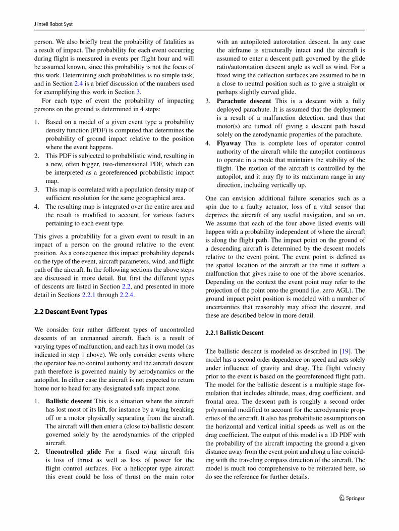
Fig. 8 Flight path altitude as AGL. The read dots show the location of the waypoins
of the flight path than this only gives negligibly differentresults. Similar considerations lead to the sample density ofthe parachute descent and uncontrolled glide to be set at 50and 100 m, respectively, with population density samplingsof 100 m by 100 m and 250 m by 250 m, respectively. Theflight path sample density for a flyaway is 1000 m. The windis assumed to be normally distributed in direction and speed.The actual parameters used in the simulation are listed inTable 3.
Examples of georeferenced impact areas for each of theevent types are shown in Fig. 9 for ballistic, uncontrolledglide, and parachute, and for flyaway in Fig. 10. All fourexamples use the same event point, namely WP 39 overthe city of Silkeborg. Notice how the size of the areas varysignificantly, and all show signs of the east-north-east winddirection.
3.3 Computing Probability of Fatality Along FlightPath
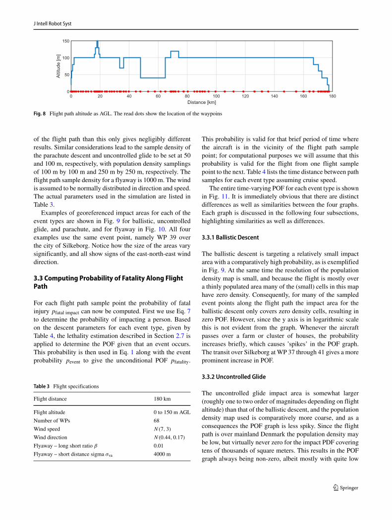
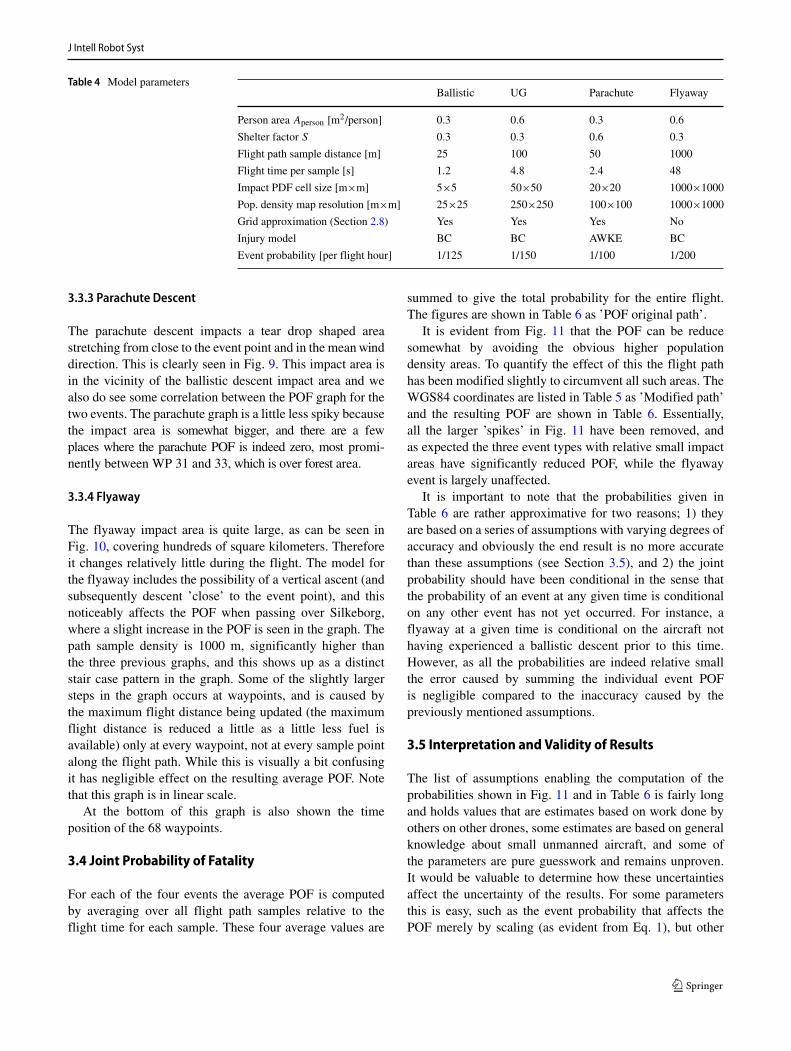
For each flight path sample point the probability of fatalinjury pfatal impact can now be computed. First we use Eq. 7to determine the probability of impacting a person. Basedon the descent parameters for each event type, given byTable 4, the lethality estimation described in Section 2.7 isapplied to determine the POF given that an event occurs.This probability is then used in Eq. 1 along with the eventprobability pevent to give the unconditional POF pfatality.
Table 3 Flight specifications
Flight distance 180 km
Flight altitude 0 to 150 m AGL
Number of WPs 68
Wind speed N(7, 3)
Wind direction N(0.44, 0.17)
Flyaway – long short ratio β 0.01
Flyaway – short distance sigma σva 4000 m
This probability is valid for that brief period of time wherethe aircraft is in the vicinity of the flight path samplepoint; for computational purposes we will assume that thisprobability is valid for the flight from one flight samplepoint to the next. Table 4 lists the time distance between pathsamples for each event type assuming cruise speed.
The entire time-varying POF for each event type is shownin Fig. 11. It is immediately obvious that there are distinctdifferences as well as similarities between the four graphs.Each graph is discussed in the following four subsections,highlighting similarities as well as differences.
3.3.1 Ballistic Descent
The ballistic descent is targeting a relatively small impactarea with a comparatively high probability, as is exemplifiedin Fig. 9. At the same time the resolution of the populationdensity map is small, and because the flight is mostly overa thinly populated area many of the (small) cells in this maphave zero density. Consequently, for many of the sampledevent points along the flight path the impact area for theballistic descent only covers zero density cells, resulting inzero POF. However, since the y axis is in logarithmic scalethis is not evident from the graph. Whenever the aircraftpasses over a farm or cluster of houses, the probabilityincreases briefly, which causes ’spikes’ in the POF graph.The transit over Silkeborg at WP 37 through 41 gives a moreprominent increase in POF.
3.3.2 Uncontrolled Glide
The uncontrolled glide impact area is somewhat larger(roughly one to two order of magnitudes depending on flightaltitude) than that of the ballistic descent, and the populationdensity map used is comparatively more coarse, and as aconsequences the POF graph is less spiky. Since the flightpath is over mainland Denmark the population density maybe low, but virtually never zero for the impact PDF coveringtens of thousands of square meters. This results in the POFgraph always being non-zero, albeit mostly with quite low

J Intell Robot Syst
Fig. 9 Impact PDFs for ballistic descent (smallest area), uncontrolledglide (largest area), and parachute descent (tear drop shaped). Eventlocation for the three impact PDFs is all at WP 39 (marked assubsampling no. 1). The blue triangles mark the uncontrolled glidesubsampling (i.e. for every 100 m of flight). The red line is the flight
direction and the green line is the mean wind direction. The highlytransparent white rectangles show the sizes of the PDF matrices andthey are geographically aligned NS-EW. The white line shows the lin-ear interpolation between waypoints. The city is Silkeborg, Denmarkand the view direction is north-east
values. The flight path was chosen to pass over a few towns(which are easily identified as short increases in the graph)as well as Silkeborg, which gives the largest increase inPOF. Notice how this increase is located earlier in time than
the corresponding increase for the ballistic descent. This iscaused by the uncontrolled glide impacting 1000 to 1500m ahead of the event point, whereas the ballistic descent isonly 50-100 m ahead.
Fig. 10 Impact PDF for a flyaway event for the aircraft fully fueled atthe start of the flight. The event location is WP 39. There is a very smallyellow zone in the middle of the concentric contour lines, which is thevertical flyaway zone. But it is too small to be visible in this view. The
highly transparent white rectangle shows the size of the PDF matrixand the white line shows the entire flight path. The view direction isdue north
J Intell Robot Syst
Table 4 Model parametersBallistic UG Parachute Flyaway
Person area Aperson [m2/person] 0.3 0.6 0.3 0.6
Shelter factor S 0.3 0.3 0.6 0.3
Flight path sample distance [m] 25 100 50 1000
Flight time per sample [s] 1.2 4.8 2.4 48
Impact PDF cell size [m×m] 5×5 50×50 20×20 1000×1000
Pop. density map resolution [m×m] 25×25 250×250 100×100 1000×1000
Grid approximation (Section 2.8) Yes Yes Yes No
Injury model BC BC AWKE BC
Event probability [per flight hour] 1/125 1/150 1/100 1/200
3.3.3 Parachute Descent
The parachute descent impacts a tear drop shaped areastretching from close to the event point and in the mean winddirection. This is clearly seen in Fig. 9. This impact area isin the vicinity of the ballistic descent impact area and wealso do see some correlation between the POF graph for thetwo events. The parachute graph is a little less spiky becausethe impact area is somewhat bigger, and there are a fewplaces where the parachute POF is indeed zero, most promi-nently between WP 31 and 33, which is over forest area.
3.3.4 Flyaway
The flyaway impact area is quite large, as can be seen inFig. 10, covering hundreds of square kilometers. Thereforeit changes relatively little during the flight. The model forthe flyaway includes the possibility of a vertical ascent (andsubsequently descent ’close’ to the event point), and thisnoticeably affects the POF when passing over Silkeborg,where a slight increase in the POF is seen in the graph. Thepath sample density is 1000 m, significantly higher thanthe three previous graphs, and this shows up as a distinctstair case pattern in the graph. Some of the slightly largersteps in the graph occurs at waypoints, and is caused bythe maximum flight distance being updated (the maximumflight distance is reduced a little as a little less fuel isavailable) only at every waypoint, not at every sample pointalong the flight path. While this is visually a bit confusingit has negligible effect on the resulting average POF. Notethat this graph is in linear scale.
At the bottom of this graph is also shown the timeposition of the 68 waypoints.
3.4 Joint Probability of Fatality
For each of the four events the average POF is computedby averaging over all flight path samples relative to theflight time for each sample. These four average values are
summed to give the total probability for the entire flight.The figures are shown in Table 6 as ’POF original path’.
It is evident from Fig. 11 that the POF can be reducesomewhat by avoiding the obvious higher populationdensity areas. To quantify the effect of this the flight pathhas been modified slightly to circumvent all such areas. TheWGS84 coordinates are listed in Table 5 as ’Modified path’and the resulting POF are shown in Table 6. Essentially,all the larger ’spikes’ in Fig. 11 have been removed, andas expected the three event types with relative small impactareas have significantly reduced POF, while the flyawayevent is largely unaffected.
It is important to note that the probabilities given inTable 6 are rather approximative for two reasons; 1) theyare based on a series of assumptions with varying degrees ofaccuracy and obviously the end result is no more accuratethan these assumptions (see Section 3.5), and 2) the jointprobability should have been conditional in the sense thatthe probability of an event at any given time is conditionalon any other event has not yet occurred. For instance, aflyaway at a given time is conditional on the aircraft nothaving experienced a ballistic descent prior to this time.However, as all the probabilities are indeed relative smallthe error caused by summing the individual event POFis negligible compared to the inaccuracy caused by thepreviously mentioned assumptions.
3.5 Interpretation and Validity of Results
The list of assumptions enabling the computation of theprobabilities shown in Fig. 11 and in Table 6 is fairly longand holds values that are estimates based on work done byothers on other drones, some estimates are based on generalknowledge about small unmanned aircraft, and some ofthe parameters are pure guesswork and remains unproven.It would be valuable to determine how these uncertaintiesaffect the uncertainty of the results. For some parametersthis is easy, such as the event probability that affects thePOF merely by scaling (as evident from Eq. 1), but other

J Intell Robot Syst
10
-8
10
-7
10
-6
10
-5
POF/h
Bal
listi
cP
robability o
ver tim
e
Average
Wa
yp
oin
ts
10
-8
10
-7
10
-6
10
-5
POF/h
Un
con
tro
lled
glid
e
10
-8
10
-7
10
-6
10
-5
POF/h
Par
ach
ute
01000
2000
3000
4000
5000
6000
7000
8000
Flig
ht tim
e (
se
co
nd
s)
3456345
POF/h 10-8
1 2 3
4 5
6 7
8 9
10
11
12
131
415161
718
19
20
21
22
23
24
25
262
72
82
93
03
13
23
33
43
53
63
73
83
94
04
14
24
34
44
54
64
74
84
95
05
15
25
35
45
55
65
75
85
96
06
16
26
36
46
56
66
76
8
Fly
away
Fig.11
POF
for
the
four
even
tty
pes
asa
func
tion
oftim
edu
ring
the
flig
ht.T
heda
shed
red
line
show
nth
eav
erag
efo
rth
een
tire
flig
ht.A
tth
ebo
ttom
ofth
eFl
yaw
aygr
aph
issh
own
the
time
loca
tion
ofth
ew
aypo
ints
.The
firs
tthr
eegr
aphs
use
loga
rith
mic
scal
e,w
hile
Flya
way
uses
linea
rsc
ale

J Intell Robot Syst
Table 5 List of WGS84 coordinates for original and modified flight paths
Original path Modified path
WP# Latitude Longitude AGL Latitude Longitude AGL
1 55.554545030296 9.479322401507 20 55.554545030296 9.479322401507 20
2 55.554680578851 9.476749600627 40 55.554680578851 9.476749600627 40
3 55.556493899011 9.472955222674 60 55.556493899011 9.472955222674 60
4 55.560772780031 9.469421045602 80 55.560772780031 9.469421045602 80
5 55.571128233980 9.467951534842 100 55.571128233980 9.467951534842 100
6 55.580554097762 9.477530540320 100 55.580699042913 9.468063130546 100
7 55.595347595425 9.475706907721 100 55.595678117696 9.469625061952 100
8 55.609464552686 9.467568767644 100 55.609464552686 9.467568767644 100
9 55.622126964138 9.457714905384 100 55.622126964138 9.457714905384 100
10 55.640033838008 9.450405736055 100 55.640033838008 9.450405736055 100
11 55.653584519126 9.455903118340 100 55.653584519126 9.455903118340 100
12 55.671544872137 9.462502164140 100 55.671544872137 9.462502164140 100
13 55.690793023267 9.452169109227 110 55.689231538618 9.443633439260 100
14 55.697841276171 9.451795763291 130 55.695241051100 9.432198928936 100
15 55.705155424780 9.452008039724 150 55.701426874904 9.424480457267 100
16 55.713342716316 9.452635295842 130 55.712808999641 9.419787857672 100
17 55.718737589467 9.453860786061 110 55.721262024323 9.424097473257 100
18 55.724870646620 9.458778087963 100 55.729548739524 9.436538591473 100
19 55.736882932082 9.458950488854 100 55.739473049343 9.448720466326 100
20 55.754978057789 9.456697504419 100 55.754043339766 9.460182361401 100
21 55.766389861392 9.457419201889 100 55.769330749294 9.460182360621 100
22 55.783061055668 9.463099739267 100 55.783061055668 9.463099739267 100
23 55.796311267866 9.471218257102 100 55.796303809176 9.462284853005 100
24 55.809546318692 9.481585537150 100 55.812623312168 9.457191361399 100
25 55.826623171859 9.489901805754 100 55.829171660912 9.453610115704 100
26 55.842014846903 9.487857577784 70 55.844880820540 9.450562706138 100
27 55.850530209601 9.487860863523 70 55.857056359990 9.446506570546 100
28 55.867137492954 9.485695418246 100 55.872292575249 9.446434322188 100
29 55.881305880608 9.482237070355 100 55.890727301460 9.453352909541 100
30 55.899312437586 9.479473303976 100 55.912650991875 9.461405525529 100
31 55.942643730522 9.469745001365 100 55.942643730522 9.469745001365 100
32 55.969530410357 9.479280816704 40 55.969530410357 9.479280816704 100
33 56.017601083823 9.466256699438 40 56.017601083823 9.466256699438 100
34 56.057808129637 9.480695780839 40 56.057808129637 9.480695780839 100
35 56.090264077707 9.508752252898 40 56.087703424994 9.473621132251 100
36 56.115225760456 9.536264547242 100 56.114624114342 9.451205789754 100
37 56.146749328129 9.541634146861 120 56.133894803581 9.429811971342 100
38 56.155659416951 9.542015090368 120 56.156304535315 9.424143409130 100
39 56.167188110346 9.541514910841 120 56.168864836335 9.430687257542 100
40 56.177444408361 9.542412101968 120 56.184127386842 9.439530367466 100
41 56.196028064574 9.542890432537 100 56.207690305472 9.449741685742 100
42 56.225366530587 9.523635840514 100 56.234891586695 9.490194574182 100
43 56.249117014960 9.543181285937 100 56.259444632292 9.518195370221 100
44 56.283498377364 9.583744503554 100 56.287405200628 9.538855144080 100
45 56.299891685624 9.582816893589 100 56.316228368282 9.543671729848 100
46 56.317290167629 9.588831148520 100 56.330044984775 9.551193442068 100
47 56.332442655605 9.584268393221 100 56.346184198871 9.557743379279 100

J Intell Robot Syst
Table 5 (continued)
Original path Modified path
WP# Latitude Longitude AGL Latitude Longitude AGL
48 56.345701312115 9.595420808242 100 56.361723383614 9.560967098869 100
49 56.369226580481 9.590604318891 100 56.387649271489 9.565681966600 100
50 56.409898900464 9.568224728466 100 56.409898900464 9.568224728466 100
51 56.467584399225 9.567370972179 100 56.467734298736 9.553529311465 100
52 56.521781127382 9.566187195270 100 56.524526113619 9.547828241131 100
53 56.581812248122 9.583664030196 100 56.580764311815 9.574936605005 100
54 56.650079997414 9.604148586681 100 56.648393997396 9.588440791549 100
55 56.695438580383 9.606018831192 100 56.694146568537 9.591645889909 100
56 56.732806256253 9.627111567328 100 56.754781558791 9.598422967079 100
57 56.827334617828 9.674385020774 100 56.827334617828 9.674385020774 100
58 56.900797285025 9.695550478188 100 56.900797285025 9.695550478188 100
59 56.947371874912 9.698767611715 100 56.947371874912 9.698767611715 100
60 56.981525482529 9.723820847486 100 56.970595106677 9.733897626722 100
61 56.993511801990 9.761587953247 80 56.991496077850 9.760649326777 80
62 56.991051020372 9.816935870554 60 57.013003165267 9.762891470667 60
63 56.995523555285 9.840415594179 60 57.024691896377 9.772740225473 60
64 57.001745474616 9.853392191806 40 57.042973948529 9.783842662825 40
65 57.014167025759 9.853595038740 40 57.047911099505 9.800979436634 40
66 57.023354417254 9.849206649568 40 57.046613711923 9.818299119874 40
67 57.034709513318 9.848430778663 20 57.044711999436 9.837013427784 20
68 57.043000539486 9.855678708563 0 57.043000539486 9.855678708563 0
parameters enter the computations in a highly nonlinearfashion (such as wind direction and speed). Therefore theeffect of varying such parameters is not easy to determine. Astudy of the sensitivity of the individual parameters remainsas future work.
The substantial uncertainty aside the estimated parame-ters in Table 3 and 4 have deliberately been chosen slightlyconservative to reduce the risk that the derived probabilitiesare unrealistically low. Coupled with the above considera-tions on the lack of knowledge of actual values, it is indeedlikely that POF estimates are perhaps as much as an orderof magnitude wrong. Still, the precision is within the uncer-tainty range that applies to many similar considerations formanned aviation.
4 Conclusion
The application to the example Penguin C flight from Kold-ing to Aalborg demonstrates how it is possible with theproposed methodology to quantify an estimate of the POFfor a specific flight. The computations are fully parameter-ized, and are thus easy to repeat for another flight path, foranother aircraft, for other wind parameters, etc. It is impor-tant to note that the risk assessment here does not coverall possible flight terminating events, as does it not includemidair collision and impacts with ground obstacles. Also,there might be other event types depending on the type ofaircraft. However, it is relatively easy to include additionalevents (which is certainly necessary for other aircraft types,
Table 6 Probabilities offatality per flight hour for thetwo example flights
Ballistic Uncontrolled Parachute
decent glide descent Flyaway Joint
POF for original path per flight hour 1.1 · 10−7 2.2 · 10−7 2.7 · 10−7 4.7 · 10−8 6.5· 10−7
POF for modified path per flight hour 2.1· 10−8 2.5· 10−8 4.1 · 10−8 4.7 · 10−8 1.3 · 10−7

J Intell Robot Syst
such as rotorcraft). For approval of BVLOS flights thismethod contributes in a tangible way to assist the authoritiesin determining the risk associated with a given type of flightoperation, and as indicated above the Danish Transport,Construction, and Housing Authority accepts this method as avalid tool to anyone applying for permit to conduct BVLOSoperations in Danish airspace.
There remains substantial future work to improve andrefine the method, as well as including more events, andmore types of aircraft. Also, more accuracy on assumptionswill be beneficial for the resulting probabilities.
The Penguin C aircraft is picked at random for thiswork. The author is not affiliated with UAV Factory. Theresults cannot be used ‘as is’ for a quantitative correctrisk assessment of the aircraft since some of the aircraftparameters most likely are not correct.
Acknowledgements This work is supported by the BVLOS FastTrackproject between the Danish Transport Construction and HousingAuthority, University of Southern Denmark, Aalborg University, UASTest Center Denmark, and Heliscope. We wish to thank the partnersfor providing information and data for this work.
A short version of this paper was presented in ICUAS 2017 [21].
Open Access This article is distributed under the terms of theCreative Commons Attribution 4.0 International License (http://creativecommons.org/licenses/by/4.0/), which permits unrestricteduse, distribution, and reproduction in any medium, provided you giveappropriate credit to the original author(s) and the source, provide alink to the Creative Commons license, and indicate if changes weremade.
Publisher’s Note Springer Nature remains neutral with regard tojurisdictional claims in published maps and institutional affiliations.
References
1. Scale, A.A.A.M.: (AIS) abbreviated injury manual. Technicalreport, Association for the Advancement of Automotive Medicine,2005 (2005)
2. Arterburn, D., Ewing, M., Prabhu, R., Zhu, F., Francis, D.: FAAUAS center of excellence task A4: UAS ground collision severityevaluation. Technical report, ASSURE (2017)
3. Atkins, E.M., Portillo, I.A., Strube, M.J.: Emergency flightplanning applied to total loss of thrust. J. Aircr. 43(4), 1205–1216(2006)
4. Bertrand, S., Raballand, N., Viguier, F., Muller, F.: Ground riskassessment for long-range inspection missions of railways byUAVs. In: proceedings of ICUAS 2017, pp. 1343–1351 (2017)
5. Bir, C.A., Viano, D.C.: Design and injury assessment criteria forblunt ballistic impacts. J. Trauma Injury, Infection, and CriticalCare 57, 1218–1224 (2004)
6. Clare, V.R., Mickiewicz, A.P., Lewis, J.H., Sturdiven, L.M.: Blunttrauma data correlation technical report report may EB-TR-75016Edgewood Arsenal (1975)
7. Clothier, R., Walker, R., Fulton, N., Campbell, D.: A casualtyrisk analysis for unmanned aerial system (UAS) operationsover inhabited areas. In: 2nd Australasian unmanned air vehicleconference, pp. 1–15 (2007)
8. Clothier, R., Williams, B., Washington, A.: Development of aTemplate Safety Case for Unmanned Aircraft Operations OverPopulous Areas. In: SAE 2015 AeroTech Congress & Exhibition,pp. 10 (2015)
9. Clothier, R.A., Walker, R.A.: The safety risk management ofunmanned aircraft systems. In: Valavanis, K.P., Vachtsevanos,G.J. (eds.) Handbook of unmanned aerial vehicles, p. 37. SpringerScience + Business Media B.V., Dordrecht (2013)
10. Clothier, R.A., Williams, B.P., Fulton, N.L.: Structuring the safetycase for unmanned aircraft system operations in non-segregatedairspace. Saf. Sci. 79, 213–228 (2015)
11. Coombes, M., Chen, W.-H., Render, P.: Landing site reachabilityin a forced landing of unmanned aircraft in wind journal ofaircraft, pp. 1–13 (2017)
12. Dalamagkidis, K., Valavanis, K.P., Piegl, L.A.: On unmannedaircraft systems issues, challenges and operational restrictionspreventing integration into the national airspace system. Prog.Aerosp. Sci. 44(7-8), 503–519 (2008)
13. Denney, E., Pai, G.: Architecting a safety case for UAS flightoperations. In: 34th international system safety conference, pp. 12(2016)
14. Denney, E., Pai, G., Habli, I.: Perspectives on software safetycase development for unmanned aircraft Proceedings of theinternational conference on dependable systems and networks(2012)
15. Freeman, P., Gary J Balas.: Actuation failure modes effectsanalysis for a small UAV. In: actuation failure American controlconference, pp. 1292–1297. IEEE (2014)
16. Freeman, P.M.: Reliability assessment for low-cost unmannedaerial vehicles. PhD thesis, University of Minneota (2014)
17. Guglieri, G., Ristorto, G.: Safety assessment for light remotelypiloted aircraft systems. In: 2016 INAIR - international conferenceon air transport, pp. 1–7 (2016)
18. King, D.W., Bertapelle, A., Moses, C.: UAV failure rate criteriafor equivalent level of safety. In: International helicopter safetysymposium, pp. 9, Montreal (2005)
19. la Cour-Harbo, A.: Ground impact probability distributionfor small unmanned aircraft in ballistic descent. Reliabilityengineering and system safety Submitted (2017)
20. la Cour-Harbo, A.: Mass threshold for ’harmless’ drones.International Journal of Micro Air Vehicles, pp. 11 (2017)
21. la Cour-Harbo, A.: Quantifying risk of ground impact fatalitiesof power line inspection BVLOS flight with small unmannedaircraft. In: 2017 International Conference on Unmanned AircraftSystems (ICUAS), pp. 1352–1360 (2017)
22. Lin, X., Fulton, N.L., Horn, M.E.T.: Quantification of high levelsafety criteria for civil unmanned aircraft systems. In: IEEEaerospace conference proceedings, pp. 13 (2014)
23. Murtha, J.F.: An evidence theoretic approach to design of reliablelow-cost UAVs. PhD thesis, Virginia Polytechnic Institute (2009)
24. Office of the Secretary of Defence: Unmanned aerial vehiclereliability study. Technical report february, Department of defense(2003)
25. Radi, A.: Human injury model for small unmanned aircraftimpacts. Technical report, Civil aviation safety authority, Australia(2013)
26. Reimann, S., Amos, J., Bergquist, E., Cole, J., Phillips, J., Shuster,S.: UAV for reliability technical report december AEM 4331aerospace vehicle design (2013)
27. Reimann, S., Amos, J., Bergquist, E., Cole, J., Phillips, J., Shuster,S.: UAV for Reliability Build. University of Minnesota, Technicalreport (2014)
28. Larry, M., Viano, S.C., Champion, H.R.: Analysis of injurycriteria to assess chest and abdominal injury risks in blunt andballistic impacts. J. Trauma 56(3), 651–663 (2004)

J Intell Robot Syst
29. Twisdale, L.A., Vickery, P.J.: Comparison of debris trajectorymodels for explosive safety hazard analysis. In: 25th DoD Explo-sive Safety Seminar Anaheim, California, pp. 513–526 (1992)
30. Venkataraman, R.: Reliability assessment of actuator architecturesfor unmanned aircraft. University of Minnesota, PhD thesis (2015)
31. Venkataraman, R., Lukatsi, M., Vanek, B., Seiler, P.: Reliabilityassessment of actuator architectures for unmanned aircraft. IFAC-PapersOnLine 48(21), 398–403 (2015)
32. Viano, D.C., Lau, I.A.N.V.: A viscous tolerance criterion for softtissue injury assessment. J. Biomech. 21(5), 387–399 (1988)
33. Warren, M., Mejias, L., Kok, J., Yang, X., Gonzalez, F., Upcroft,B.en.: An automated emergency landing system for fixed-wingaircraft: Planning and control. J. Field Rob. 32(8), 1114–1140(2015)
34. Warren, M., Mejias, L., Yang, X., Arain, B., Gonzalez, F.,Ben Upcroft.: Enabling aircraft emergency landings using activevisual site detection. In: Field and Service Robotics, pp. 167–181Springer Tracts in Advanced Robotics, pp. 105 (2015)
35. Paul, W.U., Clothier, R.: The development of ground impactmodels for the analysis of the risks associated with unmannedaircraft operations over inhabited areas: Inproceedings of the 11thProbabilistic Safety Assessment and Management Conference(PSAM11) and the Annual European Safety and ReliabilityConference (ESREL 2012), pp. 14 (2012)
Anders la Cour-Harbo is associate professor at Aalborg University,Dept. of Electronic Systems and Manager of AAU Drone ResearchLab. He has a MSc in mathematics from 1998 and PhD in electronicengineering from 2002. His main research interests are guidance,control, modeling, and estimation of UAS, safety computations andoperational safety for UAS, trajectory generation and flight operationsin real environment. In addition, he is certified drone pilot, androutinely operates larger rotorcraft drones.