quantifying terrestrial habitat loss and fragmentation: a
TRANSCRIPT

12 August, 2005Kevin McGarigalDepartment of Natural Resources ConservationUniversity of Massachusetts304 Holdsworth Natural Resources CenterBox 34210Amherst, MA 01003(413)545-4358 Fax(413)577-0655 Phone
Quantifying Terrestrial Habitat Loss and Fragmentation: AProtocol
Kevin McGarigalNatural Resources Conservation Department, University of Massachusetts, Amherst, MA01003. Email: [email protected]
Sam CushmanUSDA Forest Service, Rocky Mountain Research Station, Missoula, MT 59807. Email:[email protected]
Claudia ReganUSDA Forest Service, Rocky Mountain Region,, Denver, CO. Email: [email protected]
iiFragmentation Protocol
Abstract
Anthropogenic habitat loss and fragmentation have been implicated as among the key driversof the burgeoning global biodiversity crisis. In response, there is a growing mandate amongnatural resource managers to evaluate the impacts of proposed management actions on the extentand fragmentation of habitats. Unfortunately, few guidelines exist to help managers understandthe many complex issues involved in the quantitative assessment of habitat loss andfragmentation. In our Primer, we explore habitat fragmentation as a landscape-level process inwhich a specific habitat is progressively sub-divided into smaller, geometrically altered, andmore isolated fragments as a result of both natural and human activities. We describe alternativeperspectives on fragmentation in which habitat patches are viewed either as analogs of oceanicislands embedded in an ecologically neutral sea or as patches of variable quality embeddedwithin a complex and heterogeneous mosaic of patches of varying suitability and affects onhabitat connectivity. In the conventional island biogeographic perspective, habitat loss andfragmentation is described as a landscape transformation process involving several recognizablephases that are demarcated by significant changes in the pattern or function of the landscape. Wedescribe the key spatial components of habitat loss and fragmentation: habitat extent,subdivision, geometry, isolation, and connectivity, and their affects on individual behavior andhabitat use, population structure and viability, and interspecific interactions. Finally, we view theevidence, both theoretical and empirical, regarding the issue of when is habitat fragmentationimportant, and conclude that it depends not only on the pattern of habitat distribution but on thelife history characteristics (e.g., dispersal capabilities) of the target organism(s).
The Primer on habitat fragmentation provides the foundation for examining several keyissues in the analysis of habitat loss and fragmentation. First, what constitutes habitat. Second,how do we represent landscape structure in a digital data model. Third, what are the componentsof habitat loss and fragmentation. Fourth, what is the appropriate scale of analysis, Fifth, what isthe relevant spatiotemporal context for assessing habitat loss and fragmentation. Finally, how arehabitat loss and fragmentation measured.
The conceptual overview (i.e., Primer) on habitat fragmentation and discussion of importantanalytical issues provides the foundation for a step-by-step protocol for quantitatively assessinghabitat loss and fragmentation. This protocol consists of five steps and is intended to serve as ageneral guideline for the quantitative assessment process, but one that must be tailored to meetthe specific conditions of any particular application.

1Fragmentation Protocol
TABLE OF CONTENTS
PURPOSE AND ORGANIZATION . . . . . . . . . . . . . . . . . . . . . . . . . . . . . . . . . . . . . . . . . . . . . . . 1
A PRIMER ON HABITAT FRAGMENTATION . . . . . . . . . . . . . . . . . . . . . . . . . . . . . . . . . . . . 3What is Habitat Fragmentation? . . . . . . . . . . . . . . . . . . . . . . . . . . . . . . . . . . . . . . . . . . . . . . . 3Habitat Fragmentation Paradigms . . . . . . . . . . . . . . . . . . . . . . . . . . . . . . . . . . . . . . . . . . . . . . 7
Static Island Biogeographic Model . . . . . . . . . . . . . . . . . . . . . . . . . . . . . . . . . . . . . . . . . . 7Dynamic Landscape Mosaic Model . . . . . . . . . . . . . . . . . . . . . . . . . . . . . . . . . . . . . . . . . 10
Spatial Components of Habitat Fragmentation . . . . . . . . . . . . . . . . . . . . . . . . . . . . . . . . . . . 11Biological Consequences of Habitat Fragmentation . . . . . . . . . . . . . . . . . . . . . . . . . . . . . . . 14
Individual Behavior and Habitat Use . . . . . . . . . . . . . . . . . . . . . . . . . . . . . . . . . . . . . . . 15Population Structure and Viability . . . . . . . . . . . . . . . . . . . . . . . . . . . . . . . . . . . . . . . . . 23Interspecific Interactions . . . . . . . . . . . . . . . . . . . . . . . . . . . . . . . . . . . . . . . . . . . . . . . . . 28
When is Habitat Fragmentation Important? . . . . . . . . . . . . . . . . . . . . . . . . . . . . . . . . . . . . . . 29Implications for National Forest Management . . . . . . . . . . . . . . . . . . . . . . . . . . . . . . . . . . . 31
ISSUES IN THE QUANTITATIVE ANALYSIS OF HABITAT LOSS ANDFRAGMENTATION . . . . . . . . . . . . . . . . . . . . . . . . . . . . . . . . . . . . . . . . . . . . . . . . . . . . . . . . . . 34
What is the Appropriate Model of Landscape Structure? . . . . . . . . . . . . . . . . . . . . . . . . . . . 34What is the Appropriate Scale of Analysis? . . . . . . . . . . . . . . . . . . . . . . . . . . . . . . . . . . . . . 36What is the Relevant Spatiotemporal Context for Assessing Habitat Loss and Fragmentation?
. . . . . . . . . . . . . . . . . . . . . . . . . . . . . . . . . . . . . . . . . . . . . . . . . . . . . . . . . . . . . . . . . . . . . 39What are the Best Measures of Habitat Loss and Fragmentation? . . . . . . . . . . . . . . . . . . . . 40
A PROTOCOL FOR ASSESSING HABITAT LOSS AND FRAGMENTATION . . . . . . . . . . 49Illustrated Example . . . . . . . . . . . . . . . . . . . . . . . . . . . . . . . . . . . . . . . . . . . . . . . . . . . . . 49
Step 1: Establish Analysis Objectives . . . . . . . . . . . . . . . . . . . . . . . . . . . . . . . . . . . . . . . . . . 51Illustrated Example . . . . . . . . . . . . . . . . . . . . . . . . . . . . . . . . . . . . . . . . . . . . . . . . . . . . . 52
Step 2: Define the Landscape . . . . . . . . . . . . . . . . . . . . . . . . . . . . . . . . . . . . . . . . . . . . . . . . 53Illustrated Example . . . . . . . . . . . . . . . . . . . . . . . . . . . . . . . . . . . . . . . . . . . . . . . . . . . . . 55
Step 3: Establish a Spatio-Temporal Reference Framework . . . . . . . . . . . . . . . . . . . . . . . . . 57Illustrated Example . . . . . . . . . . . . . . . . . . . . . . . . . . . . . . . . . . . . . . . . . . . . . . . . . . . . . 58
Step 4: Quantify Habitat Fragmentation . . . . . . . . . . . . . . . . . . . . . . . . . . . . . . . . . . . . . . . . 61Illustrated Example . . . . . . . . . . . . . . . . . . . . . . . . . . . . . . . . . . . . . . . . . . . . . . . . . . . . . 61
Step 5: Characterize the Landscape Relative to Analysis Objectives . . . . . . . . . . . . . . . . . . 68Illustrated Example . . . . . . . . . . . . . . . . . . . . . . . . . . . . . . . . . . . . . . . . . . . . . . . . . . . . . 69
ACKNOWLEDGMENTS . . . . . . . . . . . . . . . . . . . . . . . . . . . . . . . . . . . . . . . . . . . . . . . . . . . . . . 71
LITERATURE CITED . . . . . . . . . . . . . . . . . . . . . . . . . . . . . . . . . . . . . . . . . . . . . . . . . . . . . . . . 72
FIGURE CAPTIONS . . . . . . . . . . . . . . . . . . . . . . . . . . . . . . . . . . . . . . . . . . . . . . . . . . . . . . . . . 110

2Fragmentation Protocol
PURPOSE AND ORGANIZATION
Many scientists believe that the earth is facing a mass extinction (Lawton and May 1995,Vitousek et al. 1997, Wilson 1999, Myers and Knoll 2001, Balmford et al. 2003). Current globalextinction rates for animals and plants are as much as 1,000 times higher than the backgroundrate in the fossil record (Wilson 1999) and vertebrate animal taxa are disappearing atdisproportionately high rates (Baillie et al. 2004). Anthropogenic habitat loss and fragmentationhave been implicated as among the key drivers of this global biodiversity crisis (Wilcox andMurphy 1985, Saunders et al. 1991, Andren 1994, Myers and Knoll 2001, Balmford et al. 2003).In response, there is a growing mandate for natural resource managers to evaluate the impacts ofproposed management actions on the extent and fragmentation of habitats (Fahrig and Merriam1985, Lubchenco et al. 1991, Hobbs 1993). For example, habitat fragmentation is currently listedby the Chief of the Forest Service as one of the "four threats" of greatest concern in managementof National Forest Lands. Unfortunately, few guidelines exist to help managers understand themany complex issues involved in the quantitative assessment of habitat loss and fragmentation.
The main purpose of this document is to describe a protocol for quantitatively assessingterrestrial habitat loss and fragmentation. While the theoretical framework and conceptspresented here are broadly applicable to any ecological system, the focus here is on terrestrialhabitats in forested landscapes of North America. The motivation for this document, in part,stemmed from two regional conferences on forest fragmentation. The first conference entitled"Forest Fragmentation: Wildlife and Management Implications" was held in Portland, Oregon on18-19 November, 1998. The conference was convened to provide a synthesis of the current stateof knowledge related to fragmentation in managed forests of the Pacific Northwest and resultedin an edited book (Rochelle et al. 1999). The second conference entitled "Forest Fragmentationin the Southern Rocky Mountains" was held in Fort Collins, Colorado on ??-?? ??, 1999. Theconference was similarly convened to provide a synthesis of the current state of knowledgerelated to fragmentation in forests of the southern Rocky Mountains and also resulted in anedited book (Knight et al. 2000). While the material presented at these conferences and in thesubsequent books clearly demonstrated the rapid growth in our scientific understanding offragmentation, it was clear that managers lack clear guidelines for implementing these scientificprinciples. The purpose of this document is to help bridge that gap between science andmanagement in regard to habitat loss and fragmentation.
This document is organized into three major sections. The first section provides a primer onhabitat fragmentation. Specifically, what is habitat fragmentation, what causes it, why it isimportant, and when does it matter? An understanding of the concepts presented in this section isprerequisite to full comprehension and appreciation of the material presented in the subsequentsections. The second section discusses several key issues in the analysis of habitat loss andfragmentation. Specifically, what constitutes habitat; how do we represent landscape structure ina digital data model; what are the components of habitat loss and fragmentation; what is theappropriate scale of analysis; what is the relevant spatiotemporal context for assessing habitatloss and fragmentation; and how are habitat loss and fragmentation measured? These twosections are designed to provide the conceptual framework needed to undertake a quantitative

3Fragmentation Protocol
assessment of habitat loss and fragmentation. The third and final section presents a step-by-stepprotocol for quantitatively assessing habitat loss and fragmentation, and is illustrated with anexample from southwest Colorado.
A PRIMER ON HABITAT FRAGMENTATION
"Habitat fragmentation" has become a standard label used by conservation biologists incharacterizing human-induced ecological degradation of the environment, despite that fact thatthe notion of "habitat fragmentation" is conceptually ambiguous (Haila 1999, Fahrig 2003). Itmixes together several different but often confounded ecological processes, chief among themreduction in habitat area and change in habitat configuration (Fahrig 2003). Furthermore, as allnatural environments are "fragmented" to a variable degree, both spatially and temporally, theassessment of human-caused fragmentation is much less straightforward than it is usuallyassumed. And to further complicate matters, despite the burgeoning literature on fragmentation,adequate empirical data on the actual effects of habitat fragmentation are amazingly scarce.
What is Habitat Fragmentation?
Despite decades of attention in the scientific literature and widespread application inconservation and management, there still is no consensus on the definition of "habitatfragmentation." In part, complacency on the part of the scientific community has impeded thedevelopment of a clear and precise definition. On the other hand, the lack of consensus alsoreflects genuine disagreement among scientists and conservationists on the proper definition.Perhaps most of all, however, it reflects the natural evolution of an ecological concept.
According to the dictionary, "fragmentation" means "the breaking apart or up into pieces"(Merriam-Webster Inc. 1987). It follows, then, that "habitat fragmentation" means the breakingapart of habitat into pieces. Unfortunately, this definition doesn't apply perfectly to habitatfragmentation in the real world. Using the analogy given by Fahrig (2000), when a porcelainvase is "fragmented", the amount of porcelain remains constant. Yet, habitat fragmentationgenerally occurs through a process of habitat removal, because the total area under considerationremains constant while the total area of habitat is reduced. Therefore, habitat loss andfragmentation per se (i.e., the subdivision of habitat into isolated fragments) are inextricablylinked in real-world landscapes. It is worth noting, however, that it is possible to have habitatfragmentation without net loss of habitat under special conditions; specifically, when habitat lossis perfectly balanced against the creation of habitat through successional processes or restorationefforts. However, the more typical scenario is one of habitat fragmentation accompanied bysimultaneous habitat loss, and for this reason, some authors have chosen to consider bothcomponents under the auspices of the term "fragmentation."
Distinguishing effects of habitat fragmentation from those due to habitat loss has importantimplications for conservation biology. As Fahrig (1997) notes, "if habitat (fragmentation) isimportant, then within some limits it should be possible to mitigate effects of habitat loss by

4Fragmentation Protocol
ensuring that remaining habitat is not fragmented. On the other hand, if the effects offragmentation are trivial in comparison to effects of habitat loss, then the assumption that losscan be mitigated by reduced fragmentation has potentially dangerous consequences forconservation. If, for example, species go extinct mainly because of habitat loss, the solution isstraightforward: habitat conservation and restoration. On the other hand, if species go extinctmainly because of the fragmentation or 'breaking apart' of habitat, the problem may appear lesssevere and at the same time more complex, and the solution seems less obvious. One might evenconclude that: (1) loss of habitat is not a serious threat to species survival, as long as theremaining habitat is not broken apart; and (2) to restore endangered populations we need notrestore large tracts of habitat, but just enough to connect up the 'broken apart' pieces ofremaining habitat." Clearly, in light of these potentially erroneous conclusions, the precisedefinition of "habitat fragmentation" is not simply an issue of semantics.
For these and other reasons, the simple dictionary definition of "fragmentation" given aboveis simply inadequate to describe the complex, real-world changes that landscapes undergo duringthe fragmentation process. In particular, this definition fails to explicitly identify the scale andcomponents of the fragmentation process, as well as the causes and consequences of this process.These additional shortcomings have fostered a great deal of confusion over what is meantexactly by the term "fragmentation." For our purposes, we will define habitat fragmentation asfollows:
"Habitat fragmentation is a landscape-level process in which a specific habitat isprogressively sub-divided into smaller, geometrically altered, and more isolated fragments asa result of both natural and human activities, and this process involves changes in landscapecomposition, structure, and function at many scales and occurs on a backdrop of a naturalpatch mosaic created by changing landforms and natural disturbances (McGarigal andMcComb 1999)."
The above definition highlights the complexity of the fragmentation concept and makesexplicit the following important considerations:
First, habitat fragmentation is a 'process' of landscape change. It is not a state or condition ofthe landscape at any snapshot in time, even though it is often meaningful to substitute space fortime and compare the relative fragmentation of habitats among landscapes. Strictly speaking,however, habitat loss and fragmentation involve the progressive reduction and subdivision ofhabitat over time, which results in the alteration of landscape structure and function. Thistransformation process can be complex; it involves a number of physical changes in landscapestructure and can proceed in different patterns and at different rates depending on the causalagent (e.g., natural disturbances, agricultural clearing, timber harvesting) and the ecologicalcharacteristics of the landscape. In other words, there are multiple possible scenarios oflandscape transformation associated with fragmentation processes.
Second, habitat fragmentation is a landscape-level process, not a patch-level process. That is,fragmentation alters the spatial configuration of habitat patches within a broader habitat mosaic
5Fragmentation Protocol
or landscape, not merely the characteristics of a single patch (Fig. 1). Thus, although individualpatches are affected by fragmentation (mainly through isolation from other patches), it is theentire landscape mosaic that is transformed by the fragmentation process. Unfortunately, failureto recognize this distinction has pervaded the "fragmentation" literature for decades (McGarigaland Cushman 2002). This failure is largely due to the fact that the fragmentation concept aroseout of island biographic theory, which predicted that species number was a function of island (orpatch) size and isolation (MacArthur and Wilson 1967). Quite simply, the theory predicts thatsmaller and more isolated islands will contain fewer species due to a tradeoff betweencolonization and extinction processes. Despite the many identified shortcomings of the theory,early empirical data lent support to its simple predictions. Thus, although the original theory wasapplied to true oceanic islands, the theory was quickly extrapolated to patches in a land mosaic,and it was theorized that the reduction in patch size and increased isolation associated withhabitat loss and subdivision in landscapes undergoing agricultural and urban development wouldlead to a steady loss of species.
Failure to distinguish between island biogeography and fragmentation has led to seriousconfusion over the definition of habitat fragmentation and, perhaps more than any other issue,has clouded the conservation debate over the relative importance of habitat loss andfragmentation. Island biogeography, as applied to habitat patches in a land mosaic, involves therelationship between species richness or abundance and a variety of 'patch' characteristics, suchas patch size and isolation. Specifically, the theory predicts that small and isolated habitatpatches (i.e., area and isolation effects, respectively) will contain fewer species than large andless isolated habitat patches, and the empirical evidence for these effects is widespread (e.g.,Dodd 1990, Robinson 1992, van Apeldoorn et al. 1992, Andren 1994, Celada et al. 1994, Hunteret al. 1995, Hinsley et al. 1996, Schmiegelow et al. 1997, Vos and Chardon 1998, Fahrig 2003).The predictions of island biogeographic theory have obvious conservation implications: largeand "connected" habitat patches are likely to support viable populations of more species thansmall and isolated patches. Thus, island biogeography deals exclusively with processes operatingat the patch level: An individual patch can be progressively reduced in size and, as aconsequence, become more isolated over time, and the biological consequences of these changesare the subject of island biogeography (Fig. 1).
Habitat fragmentation, on the other hand, involves the subdivision of contiguous habitat intoseveral pieces (Fig. 1). The biological consequences of the fragmented (subdivided) distributionof habitat patches across the landscape is the subject of fragmentation research. Thus, in contrastto island biogeography, fragmentation explicitly deals with processes operating at the landscapelevel. This does not imply that studying patch-level processes, such as island biogeography, isnot relevant to the study of fragmentation. Quite the contrary. Understanding these patch-levelprocesses allows us to understand some of the mechanisms contributing to fragmentation effectsat the landscape level. However, relationships derived at the patch level can not be extrapolatedto infer effects of habitat fragmentation (McGarigal and Cushman 2002). It is analogous to tryingto understand metapopulation dynamics (a landscape-level process) by studying only one of thesubpopulations (patch-level). Indeed, it is widely recognized that extrapolating findings acrossspatial scales, especially patch-level to landscape-level scales, can lead to erroneous conclusions

6Fragmentation Protocol
(Wiens et al. 1987 and 1993; Wiens 1989a,b; McGarigal and McComb 1995, 1999; Villard et al.1999, Cushman and McGarigal 2004).
Third, habitat fragmentation is a habitat-specific process. That is, fragmentation occurs onlyin reference to a specific habitat. Landscapes don't undergo fragmentation, habitats withinlandscapes do. Since habitat is an organism-specific concept, the target habitats must becharacterized in ways relevant to the organism(s) under consideration. For example, the targethabitat might be forest, spruce-fir (Picea-Abies) forest, or 'old growth' spruce-fir forest. Thechoice of classification resolution should be driven by habitat specificity of the organism(s)under consideration. Attention to the resolution at which community types are distinguished iscrucial because the fragmentation trajectory within the same landscape can differ markedlyamong habitats in relation to habitat specificity. For example, in some Pacific Northwest (PNW)landscapes, old-growth Douglas-fir (Pseudotsuga menziesii) forest has been highly fragmentedby logging, yet late-seral forest (a broader, more inclusive classification) remains abundant andhighly connected (McGarigal and McComb 1995). In addition, it is important to recognize thatsince organisms perceive and respond to habitats differently, not all organisms will be affected insimilar ways by the same landscape changes. As one focal habitat undergoes fragmentation,some organisms will be adversely affected, some may actually benefit, whereas others will beunaffected.
Fourth, habitat fragmentation is a scale-dependent process, both in terms of how we(humans) perceive and measure fragmentation and in how organisms perceive and respond tofragmentation. The extent of the landscape considered, in particular, can have an importantinfluence on the measured fragmentation level; a highly fragmented habitat at one scale may becomparatively unfragmented at a much coarser (or finer) scale (e.g., when fragmented woodlotsoccur within a forested region)(e.g., McGarigal and McComb 1995). In addition, for habitatfragmentation to be consequential, it must occur at a scale (both extent and grain) that isfunctionally relevant to the organism(s) under consideration. Yet more often than not, we do notknow how organisms scale the environment (Wiens 1989, With 1994). The lack ofcorrespondence between the scale at which we measure fragmentation and the scale at whichorganisms perceive and respond to fragmentation is a great challenge to our understanding.
Fifth, habitat fragmentation results from both natural and anthropogenic causes. Here, weexplicitly recognize that habitats can be fragmented by natural causes as well as by a variety ofhuman activities. From a conservation perspective, we are primarily interested in anthropogenicchanges that cause the landscape to reside outside its expected range of natural variability, andthe adverse impacts that this may have on organisms. Accordingly, most studies have focused onanthropogenic causes and ignored the backdrop of the natural patch mosaic created by changinglandforms and natural disturbances.
The cause of fragmentation can dramatically influence the fragmentation process itself.Fragmentation caused by development, for example, usually results in a progressive andpermanent loss and fragmentation of habitat; that is, habitat is permanently lost to developmentand remnant habitat patches effectively become isolated from each other as they are embedded in

7Fragmentation Protocol
an inhospitable matrix of nonhabitat. Much of the fragmentation dogma, for example, stems fromfield studies conducted in the eastern deciduous forest of North America on forest fragmentationcaused by agricultural development and urbanization (i.e., land type conversions; e.g., Whitcombet al. 1981, Robbins et al. 1989, Terborgh 1989). Commercial timber management, on the otherhand, alters landscape structure by changing the areal extent and configuration of plantcommunities and seral stages across the landscape, and this usually occurs on a backdrop of anatural patch mosaic created by changing landforms and natural disturbances (Swanson et al.1988). Commercial timber management is considered the major cause of late-seral forest lossand fragmentation in many forested landscapes (Lehmkuhl and Ruggiero 1991, Hunter et al.1995, McGarigal and McComb 1995, Schmiegelow et al. 1997, Shinneman and Baker 2000). Anatural forest landscape is a spatially and temporally dynamic mosaic of forest patches (i.e.,shifting mosaic) driven by natural disturbances (e.g., fire and windthrow) and forest regrowth. Itis the scale and structure of this mosaic that is dramatically altered by timber managementactivities (Swanson et al. 1990). Vertebrate population responses in forested landscapes alteredby timber management activities are likely to differ from those in landscapes experiencingurbanization and agricultural development. Sharp forest/nonforest edges are transient inmanaged forest landscapes because of forest regrowth, and regenerating forest does not functionas nonhabitat for many species, but rather as habitat of variable quality and permeability toanimal movements. Late-seral forest patches may never be truly isolated or may be isolated foronly a brief period of years. Moreover, vertebrate populations in dynamic forest landscapes haveevolved in naturally heterogeneous environments and may have adaptations for coping withsome of the ecological changes associated with habitat fragmentation. For these reasons, it isquestionable whether all of the empirical findings on forest fragmentation from urban oragricultural landscapes extend to dynamic forest landscapes undergoing fragmentation by timbermanagement (Hejl 1992).
Unfortunately, similar attention has not been given to forest fragmentation caused by naturaldisturbances. Yet, it is increasingly clear that coniferous forest landscapes in western NorthAmerica are naturally highly dynamic, and that many forested habitats periodically experiencerapid fragmentation and recovery following large fires (Romme and Despain 1989, Wallin et al.1996, Knight and Reiners 2000, Veblen 2000). Anthropogenic disturbances, such as logging,primarily affect the scale, rate, and pattern of fragmentation in such landscapes. It is still unclearhow native fauna in such landscapes are affected by additional anthropogenic fragmentationcaused by timber harvesting.
Habitat Fragmentation Paradigms
To appreciate the range of current scientific thinking about habitat fragmentation one mustrecognize that there are several distinct perspectives representing different conceptualizations oflandscape structure and change (Wiens 1994, With 1999). These perspectives largely differ inhow the focal habitat is perceived and represented relative to other landscape elements, andwhether the landscape structure is viewed as relatively static (i.e., unchanging) or dynamic (i.e.,constantly changing). Although there exist many variations, two paradigms have emerged thatprovide alternative frameworks for conceptualizing the habitat loss and fragmentation process.

8Fragmentation Protocol
Static Island Biogeographic Model
The first paradigm we call the "static island biogeographic model." In this model, habitatfragments are viewed as analogues of oceanic islands in an inhospitable sea or ecologicallyneutral matrix (Fig. 2a). Under this perspective, discrete habitat patches (fragments) are seen asembedded in a uniform matrix of non-habitat. Connectivity is assessed by the size and proximityof habitat patches and whether they are physically connected via habitat corridors. The keyattributes of the model are its representation of the landscape as a binary system of habitat andinhospitable matrix, and that, once lost, habitat remains matrix in perpetuity. In extreme cases,the process of habitat loss and fragmentation continues until the target habitat is eliminatedentirely from the landscape. This scenario is perhaps best exemplified by urban sprawl andagricultural development, where remnant habitat fragments are maintained in an otherwiserelatively static matrix or are eventually eliminated entirely from the landscape.
The static island biogeography paradigm has been the dominant perspective since the inceptionof the fragmentation concept. The major advantage of the island model is its simplicity. Given afocal habitat, it is quite simple to represent the structure of the landscape in terms of habitatpatches contrasted sharply against a uniform matrix. Moreover, by considering the matrix asecologically neutral, it invites ecologists to focus on those habitat patch attributes, such as sizeand isolation, that have the strongest effect on species persistence at the patch level. The majordisadvantage of the strict island model is that it assumes a uniform and neutral matrix, which inmost real-world cases is a drastic over-simplification of how organisms interact with landscapepatterns. Not all matrix is created equal. Moreover, the strict island model usually assumes astatic landscape structure, at least with respect to the matrix. Once habitat is lost, it remainsmatrix. This, too, is not realistic in many landscapes, especially those driven by naturaldisturbances and/or forest management activities.
The landscape transformation process as conceptualized under the idealized static islandbiogeographic model can be divided into several broad stages or phases that are demarcated bysignificant changes in the pattern or function of the landscape (Forman 1995; Fig. 3). In reality,these phases are not strictly separate from each other since they may take place simultaneously;however, a dominant phase can often be identified.
1. Perforation.–Often, the first stage of habitat loss and fragmentation involves theperforation of natural habitat through direct loss, usually resulting from conversion toother land uses (e.g., agricultural clearing, housing development, timber harvesting).Perforation creates holes in otherwise contiguous habitat. Here, there is both a direct lossof habitat and a change in the spatial distribution of remaining habitat. The degree ofimpact on habitat configuration will depend on the pattern of perforation (see below).However, at this stage, the habitat is still physically well connected.
2. Dissection.–The second stage of habitat loss and fragmentation involves the dissection ofnatural habitat. In most cases, a perforated pattern will become a dissected pattern atcertain threshold levels of habitat loss. Dissection may precede or occur in conjunction
9Fragmentation Protocol
with perforation. A common route to habitat dissection is through the construction ofroads or other transportation corridors that span the landscape. In most cases, there isrelatively little reduction in habitat area caused by dissection. However, the resultinglinear landscape elements can be a significant source of disruption to the naturalcommunity because they can provide avenues for the intrusion of edge predators,invasive species, exotics, diseases and pathogens that adversely affect the organisms ofinterest. In addition, these linear elements can affect landscape connectivity by alteringmovement patterns of organisms. Perhaps most importantly, some dissecting agents suchas roads provide human access to the natural habitats and establish a network by whichfuture habitat loss and alteration will occur. Of course, as in all cases, the effects ofdissection will depend on the habitat and the organism(s) of interest.
3. Subdivision.–The third stage of habitat loss and fragmentation involves the subdivisionof habitat into disjunct patches. Forman (1995) referred to this phase as “fragmentation”,but like Jaeger (2000), who referred to this phase as “dissipation”, we prefer to use theterm fragmentation to refer to the entire sequence rather than a single phase. During thisphase, the landscape undergoes an important phase transition from a landscapecharacterized by physically connected habitat to a landscape in which the habitat isbroken up into disjunct fragments. At this point, the areal extent of habitat may still bequite large and may not yet be significantly limiting landscape function for theorganism(s) of interest. However, at this point, the habitat is physically disconnected andmay disrupt movement patterns of the target organism(s) and cause the subdivision ofpopulations into separate units. The consequences of this population subdivision will bediscussed later. Note, this phase may be confused or confounded with the “dissection”phase. The dissection phase, as idealized, typically occurs as a result of road-building inwhich the habitat is subdivided or dissected by linear features that do not result insignificant reduction in habitat area. In contrast, the subdivision phase is typicallycharacterized by concurrent habitat loss and results when the remaining habitat becomessubdivided into disjunct patches embedded within a matrix of “non-habitat.”
4. Shrinkage and Attrition.–The final stage of habitat loss and fragmentation involves theshrinkage and, in some cases, complete disappearance of the focal habitat. Here, thelandscape is in a critical state with respect to the viability of the target habitat. As habitatpatches are reduced in size and become more isolated from each other, the function of thelandscape is seriously jeopardized for organisms associated with the target habitat. Underthe island-biogeographic model, the remaining habitat fragments represent true islands inan inhospitable sea. Of course, the hostility of the matrix will depend on the organismsand how their life-history and vagility characteristics interact with landscape patterns, asdiscussed below.
This four-stage conceptualization of the landscape transformation represents an idealized andoversimplified view of habitat loss and fragmentation processes under the static islandbiogeographic model; no real landscape follows this trajectory exactly. Nevertheless, it depictsthe general sequence of events characteristic of habitats undergoing reduction and fragmentation

10Fragmentation Protocol
caused by urban and/or agricultural development. Although this simple conceptual modelprovides a useful framework, it is important to understand that there are many alternativescenarios or patterns of habitat loss and fragmentation associated with the above landscapetransformation (Fig. 4). Forman (1995) refers to such variations as “mosaic sequences.”
5. Random Model.–Habitat is lost progressively in a random pattern. Although notrepresentative of any real-world pattern of habitat loss and fragmentation, it provides auseful null model against which to compare other scenarios.
6. Contagious Model.–Habitat is lost in a contagious (i.e., aggregated) pattern. In this case,the fragmentation of habitat is controlled by the degree of contagion in the residualhabitat. Thus, under a maximum contagion scenario, the residual habitat would beaggregated into a single patch, and the habitat would not be fragmented per se.
7. Dispersed Model.–Habitat is lost in a dispersed (i.e., disaggregated) pattern. Under amaximum dispersion scenario, habitat would be perforated by dispersed ‘openings’ andwould eventually be broken into discrete fragments.
8. Edge Model.–Habitat is lost progressively in a wave-like manner, beginning on one edgeof the landscape and moving progressively across the landscape. In this scenario, there isno fragmentation of habitat per se, since the original habitat is not subdivided intodisjunct patches, but simply reduced in size steadily over time. This process is typical ofurban expansion outward from a city or some large-scale forestry operations.
9. Corridor Model.–Habitat is first bisected by corridor development (e.g., roads) and thenlost progressively outward from the corridors. In this scenario, the habitat is both reducedand fragmented. This process is typical of rural and suburban residential development inmany areas.
10. Nuclear Model.–Habitat is lost progressively from nuclei that may be dispersed in arandom, uniform, or clumped pattern. Perforations in the habitat grow steadily in size inradial fashion until eventually the habitat is subdivided (i.e., becomes disconnected). Therate and pattern of fragmentation per se will depend on the dispersion of nuclei. Thisprocess is typical of rural development and timber harvesting.
These models represent alternative patterns by which habitat may be lost from a landscape,and although idealized and oversimplified, they illustrate the wide range of possible patterns ofhabitat loss. More importantly, they illustrate the quantitative differences in habitat loss andfragmentation that can result under various scenarios (Forman 1995: page 425). For example,given the same trajectory of habitat loss, the edge model maintains the largest patches of habitatin the landscape without causing fragmentation. Conversely, the dispersed model results in thequick elimination of large patches from the landscape and, at some point, causes thefragmentation of the habitat that remains.
11Fragmentation Protocol
Dynamic Landscape Mosaic Model
The second major conceptual paradigm is the dynamic landscape mosaic model. In thisparadigm, landscapes are viewed as spatially complex, heterogeneous assemblages of covertypes, which can't be simplified into a dichotomy of habitat and matrix (Wiens et al. 1993, With2000; Fig. 2b). Rather, the landscape is viewed from the perspective of the organism. Habitatpatches are bounded by other patches that may be more or less similar (as opposed to highlycontrasting and often hostile habitats, as in the case of the island model) and the mosaic ofpatches itself changes through time in response to disturbance and succession processes.Connectivity is assessed by the extent to which movement is facilitated or impeded throughdifferent land cover types across the landscape. Land cover types may differ in their "viscosity"or resistance to movement, facilitating movement through certain elements of the landscape andimpeding it in others. This perspective represents a more holistic view of landscapes, in thatconnectivity is an emergent property of landscapes resulting from the interaction of organismswith landscape structure.
The dynamic landscape mosaic paradigm derives from landscape ecology and has onlyrecently emerged as a viable alternative to the static island biogeographic model. The majoradvantage of the landscape mosaic model is its more realistic representation of how organismsperceive and interact with landscape patterns. Few organisms exhibit a binary (all or none)response to habitat types, but rather use habitats proportionate to the fitness they confer.Moreover, movement among suitable habitat patches usually is a function of the character of theintervening habitats. Two suitable habitat patches separated by a large river may be effectivelyisolated from each other for certain organisms, regardless of the distance between them. Inaddition, the landscape mosaic model accounts for the dynamics in landscape structure due to theconstant interplay between disturbance and succession processes. This is especially important inforested landscapes where natural disturbances and timber harvesting are the major drivers oflandscape change. The major disadvantage of the landscape mosaic model is that it requiresdetailed understanding of how organisms interact with landscape structure; in particular, how thelandscape mosaic composition and configuration affect movement patterns. Unfortunately, it isexceedingly difficult in practice to collect the needed quantitative information, rendering thismodel less practical. However, even in the absence of detailed information about how targetorganisms interact with entire landscape mosaics, it is often beneficial to characterize thelandscape more realistically than as a simple binary map of habitat and matrix.
Spatial Components of Habitat Fragmentation
Whatever fragmentation paradigm one ascribes to, it is essential to understand what a givenchange in a landscape means physically. This requires explicit attention to the spatialcomponents of habitat fragmentation. Although habitat fragmentation refers simply to thesubdivision of habitat, given the above definition and discussion, it is clear that fragmentation isa complex process of change in multiple, and often correlated, components of landscapestructure. Thus, a multivariate perspective is required and it is unreasonable to expect a singlemetric, or even a few metrics, to be sufficient.
12Fragmentation Protocol
Fragmentation involves changes in both landscape composition and configuration(McGarigal and Marks 1995, Cushman and McGarigal 2002). Landscape composition refers tothe presence and amount of each habitat type within the landscape, but not the placement orlocation of habitat patches within the landscape mosaic. Landscape configuration refers to thespatial character and arrangement, position, orientation, and shape complexity of patches in thelandscape. We recognize five major components of landscape composition and configurationaffected by habitat loss and fragmentation, even though the distinctions among these componentscan be somewhat blurry at times.
1. Habitat Extent.–As noted previously, habitat loss and fragmentation are almost alwaysconfounded in real-world landscapes. Therefore, it is essential that habitat extent beconsidered in conjunction with any assessment of habitat fragmentation. Indeed, asdescribed later, it is difficult, and in some cases impossible, to interpret manyfragmentation metrics without accounting for habitat extent. Habitat extent represents thetotal areal coverage of the target habitat in the landscape and is a simple measure oflandscape composition.
2. Habitat Subdivision.–Habitat fragmentation fundamentally involves the subdivision ofcontiguous habitat into disjunct patches, which affects the overall spatial distribution orconfiguration of habitat within the landscape. Subdivision explicitly refers to the degreeto which the habitat has been broken up into separate patches (i.e., fragments), not thesize, shape, relative location, or spatial arrangement of those patches. Because these latterattributes are usually affected by subdivision, it is difficult to isolate subdivision as anindependent component.
3. Patch Geometry.–Habitat fragmentation alters the geometry, or spatial character, ofhabitat patches. Specifically, as patches are subdivided via habitat loss (Figs. 3-4), theybecome smaller, contain proportionately less core area (i.e., patch area after removing thearea within some specified edge-influence distance), typically extend over less area, andoften have modified shapes, although the nature of the change may vary depending on theanthropogenic agent (e.g., Krummel et al. 1987).
4. Habitat Isolation.–Habitat fragmentation increases habitat insularity, or isolation. That is,as habitat is lost and fragmented, residual habitat patches become more isolated fromeach other in space and time. Isolation deals explicitly with the spatial and temporalcontext of habitat patches, rather than the spatial character of the patches themselves.Unfortunately, isolation is a slippery concept because there are many ways to considercontext. In the temporal domain, isolation can be considered as the time since the habitatwas physically subdivided, but this is fraught with practical difficulties. For example,rarely do we have accurate historical data from which to determine when each patch wasisolated. Moreover, given that fragmentation is an ongoing process, it can be difficult toobjectively determine at what point the habitat becomes subdivided, since this is largely afunction of scale. In the spatial domain, isolation can be considered in several ways,depending on how one measures the spatial context of a patch. The simplest measures of
13Fragmentation Protocol
isolation are based on Euclidean distance between nearest neighbors (McGarigal andMarks 1995) or the cumulative area of neighboring habitat patches (weighted by nearestneighbor distance) within some ecological neighborhood (Gustafson and Parker 1992).These measures adopt an island biogeographic perspective, as they treat the landscape asa binary mosaic consisting of habitat patches and uniform matrix. Thus, the context of apatch is defined by the proximity and area of neighboring habitat patches; the role of thematrix is ignored. However, these measures can be modified to take into account otherhabitat types in the so-called matrix and their affects on the insularity of the focal habitat.For example, simple Euclidean distance can be modified to account for functionaldifferences among organisms. The functional distance between patches clearly dependson how each organism scales and interacts with landscape patterns (With 1999); in otherwords, the same gap between patches may not be perceived as a relevant disconnectionfor some organisms, but may be an impassable barrier for others. Similarly, the matrixcan be treated as a mosaic of patch types which contribute differentially to the isolationof the focal habitat. For example, isolation can be measured by the degree of contrast(i.e., the magnitude of differences in one or more attributes between adjacent patch types)between the focal habitat and neighboring patches.
5. Connectedness.–Habitat loss and fragmentation affect the connectedness of habitat acrossthe landscape. Connectedness integrates all of the above components and involves both astructural component (i.e., the amount and spatial distribution of habitat on the landscape;also referred to as “continuity”) and a functional component (i.e., the interaction ofecological flows with landscape pattern; also referred to as “connectivity”). Structuralconnectedness refers to the physical continuity of habitat across the landscape.Contiguous habitat is physically connected, but once subdivided, it becomes physicallydisconnected. Structural connectedness is affected by habitat extent and subdivision, butalso by the spatial extensiveness of the habitat patches (Keitt et al. 1997). Specifically, ashabitat patches become smaller and more compact, they extend over less space and thusprovide for less physical continuity of habitat across the landscape. Structuralconnectedness as considered here adopts an island biogeographic perspective.
What constitutes "functional connectedness" between patches clearly depends on theorganism of interest; patches that are connected for bird dispersal might not be connectedfor salamanders. As habitat is lost and subdivided, at what point does the landscapebecome functionally “disconnected?” As With (1999) notes, “what ultimately influencesthe connectivity of the landscape from the organism’s perspective is the scale and patternof movement (i.e., scale at which the organism perceives the landscape) relative to thescale and pattern of patchiness (i.e., structure of the landscape); ...i.e., a species’ gap-crossing or dispersal ability relative to the gap-size distribution on the landscape” (Daleet al. 1994, With and Crist 1995, Pearson et al. 1996, With et al. 1997). Hence, functionalconnections might be based on: (1) strict adjacency (touching) or some thresholddistance, e.g., a maximum dispersal distance); (2) some decreasing function of distancethat reflects the probability of connection at a given distance; or (3) a resistance-weighteddistance function, e.g., where the distance between two patches is computed as the least

14Fragmentation Protocol
cost distance on a resistance surface, where each intervening location between habitatpatches is assigned a resistance value based on its permeability to movement by the focalorganism. Then various indices of overall connectedness can be derived based on thepairwise connections between patches.
Biological Consequences of Habitat Fragmentation
The habitats in which organisms live are spatially structured at a number of scales, and thesepatterns interact with organism perception and behavior to drive the higher level processes ofpopulation dynamics and community structure (Johnson et al. 1992, Wiens et al. 1993).Anthropogenic habitat loss and fragmentation disrupts these patterns and is expected to havelarge, negative effects on biodiversity (Haila 2002). A disruption in landscape structure mayinterfere with the critical ecological processes necessary for the maintenance of biodiversity andecosystem health (With 2000, Fahrig 2003). Specifically, habitat fragmentation createsdiscontinuities (i.e., patchiness) in the distribution of critical resources (e.g., food, cover, water)and environmental conditions (e.g., microclimates), and these patterns change over time inresponse to the fragmentation process. From the perspective of an organism, these discontinuitiescreate variability in the distribution of suitable habitat, where suitable habitat is the combinationof food, cover, water, and space necessary to sustain an individual. Ultimately, physical changesin the extent and connectivity of suitable habitat conditions affect many processes that influencethe behavior and spatial habitat use patterns of individuals, and alter intra- and inter-specificinteractions that influence population persistence and community structure and dynamics.
The majority of theoretical studies suggest that the effect of habitat fragmentation is weakrelative to the effect of habitat loss (Collinham and Huntley 2000, Fahrig 1997, Henein et al.1999, Flather and Bevers 2002), although some predict larger effects (Boswell et al. 1998,Burkey 1999, Hill and Caswell 1999, Urban and Keitt 2001). In addition, some theoreticalstudies suggest that the effects of fragmentation per se should become apparent only at lowlevels of habitat amount, for example below approximately 20-30% of the landscape (Fahrig1998, Flather and Bevers 2002), although there is little empirical evidence available to test thisprediction (Fahrig 2003).
The results of empirical studies of habitat fragmentation are often difficult to interpretbecause many studies fail to address habitat fragmentation at the landscape-level, and most donot distinguish between habitat loss and habitat fragmentation (McGarigal and Cushman 2002,Fahrig 2003). Fragmentation is a landscape-level process and its effects cannot be resolvedthrough studies focusing on patches or those that do not separate area from configuration effects.However, empirical studies clearly suggest that habitat loss has large, consistently negativeeffects on biodiversity (Fahrig 2003). The effects of habitat fragmentation often are weaker, andthese effects are as likely to be positive as negative (Fahrig 2003). Because the effects of habitatfragmentation per se are weaker than those of habitat loss, to reliably measure the effects offragmentation it is necessary to experimentally or statistically control for the effects of habitatloss (McGarigal and McComb 1995, McGarigal and Cushman 2002). Below we discuss theconsequences of habitat loss and fragmentation at three levels of biological organization:

15Fragmentation Protocol
individual, population, and community. Note, this reductionist and hierarchical organization isnot intended to imply that fragmentation effects are distinct at each level, but is done forconvenience of organization and presentation.
Individual Behavior and Habitat Use
Although there are many effects of fragmentation on individual behavior, habitat usepatterns, and intra- and inter-specific interactions, they are dominated by: (1) a reduction inhabitat area (area effects), (2) an increase in the proportion of edge-influenced habitat (edgeeffects), and (3) an increase in habitat isolation (isolation effects). Briefly, as habitat is lost fromthe landscape (without being fragmented), at some point there will be insufficient area of habitatto support a population and the species will be extirpated from the landscape (Flather and Bevers2002). In addition, as habitat is lost and fragmented, the proportion of edge-influenced habitatincreases. For some species, the area near the edge is avoided or provides lower habitat quality,thereby reducing the effective area of habitat available to the species. This effect is referred to asthe "edge effect." For edge-sensitive species, the ultimate consequence of edge effects is toaccelerate the decline of the species beyond that expected based on area relationships alone. Ashabitat is fragmented, individual habitat patches also become more isolated; that is, they becomeless connected across the landscape so that populations become subdivided and suffer theconsequences of small population size (discussed later). As a result of this isolation, individualsrealize fewer opportunities for intraspecific interactions (e.g., mate selection) that may beimportant for continued occupancy. This effect is referred to as the "isolation effect." Thecombination of area, edge, and isolation effects influence individuals during the fragmentationprocess. The following sections summarize what is known about each of these effects.
Area Effects.–Habitat loss has consistently negative effects on biodiversity (Fahrig 2003),including reductions in species richness (Findaly and Houlahan 1997, Gurd et al. 2001,Schmiegelow and Monkkonen 2002, Steffan-Dewenter et al. 2002), population declines andchanges in distribution (Best et al. 2001, Gibbs 1998, Sanchez-Zapata and Calvo 1999). Habitatloss changes the distribution of resources and can affect individual behavior and spatial activitypatterns, changing the ability of the organism to acquire the resources needed to survive andreproduce (Mangel and Clark 1986, Wiens et al. 1993). For example, from an energeticsperspective, if food resources become more patchily distributed, it may be more costly to acquirethem (Mahan and Yahner 1999). In addition, moving between disjunct resource patches toacquire food resources may involve moving through sub-optimal habitats that require higherenergetic expenditures and expose individuals to higher rates of predation (Bergin et al. 2000)reduce breeding (Kurki et al. 2000), and dispersal success (Belisle et al. 2001, With and Crist1995, With and King 1999).
Most species require at least a minimum area of habitat in order to meet all life historyrequirements (e.g., Robbins et al. 1989). Theoretical studies predict a threshold habitat levelbelow which the population cannot sustain itself (Fahrig 2001, Flather and Bevers 2002, Hill andCaswell 1999, Fahrig 2003). The amount of habitat required for species persistence depends onspecies-specific behavioral and life-history characteristics (Gibbs 1998, Vance et al. 2003), and
16Fragmentation Protocol
the effects of habitat loss on each species will depend on the interaction of its ecologicalrequirements and capabilities with the degree of habitat loss in the surrounding landscape(McGarigal and Cushman 2002, Schmiegelow and Monkkonen 2002, Fahrig 2003). Forexample, large bodied, high trophic-level species appear to be particularly vulnerable to localextinction due to habitat loss (Gibbs and Stanton 2001).
Some species require that their minimum area requirements be fulfilled in contiguous habitatpatches; in other words, the individual habitat patch must be larger than the species' minimumarea requirement for a species to occupy the patch. These species are sometimes referred to as"area-sensitive" species. For example, many neotropical migratory bird species display a markedarea-sensitivity whereby their probability of occurrence in a forest patch increases non-linearlywith the size of the patch (Lynch and Whigham 1984, Freeemark and Merriam 1986, Robbins etal. 1989, Whitcomb et al. 1981, Trzcincski et al. 1999). Some other species, however, cantolerate the subdivision of habitat patches within their home range. For example, northernspotted owls have minimum area requirements for late-seral forest that varies geographically;yet, individual spotted owls use late-seral forest that may be distributed among many patches(Lehmkuhl and Raphael 1993, Forsman et al. 1984). In either case, habitat fragmentation reducesthe size of suitable habitat patches and makes it increasingly difficult for these species to meettheir minimum area requirements. As the habitat undergoes fragmentation, the mostarea-sensitive species will be lost first. As the habitat is further fragmented, other species willdrop out according to their minimum area requirements (e.g., Robbins et al. 1989, Bender andFahrig 1998, Flather and Bevers 2002). Thus, smaller patches generally contain fewer speciesthan larger patches (Debinski and Holt 2000), and the set of species remaining in small patchesis often a predictable subset of those found in large patches in the same region (Ganzhorn andEisenbeib 2001, Kolozsvary and Swihart 1999, Vallan 2000, Fahrig 2003).
Edge Effects.–One of the most dramatic and well-studied consequences of habitatfragmentation is an increase in the proportional abundance of edge-influenced habitat. Earlywildlife management efforts were focused on maximizing edge habitat because it was believedthat most species favored habitat conditions created by edges and that the juxtaposition ofdifferent habitats would increase species diversity (Leopold 1933). Indeed this concept of edgeas a positive influence guided land management practices for most of the twentieth century.Recent studies, however, have suggested that changes in microclimate, vegetation, invertebratepopulations, predation, brood parasitism, and competition along forest edges (i.e., edge effects)has resulted in the population declines of several vertebrate species dependent upon forestinterior conditions (e.g., Strelke and Dickson 1980, Kroodsma 1982, Brittingham and Temple1983, Wilcove 1985, Temple 1986, Noss 1988, Yahner and Scott 1988, Robbins et al. 1989,Hoover et al. 1995, Laurence et al. 2002). In fact, many of the adverse effects of forestfragmentation on organisms seem to be directly or indirectly related to these so-called edgeeffects. In contrast, some species appear to respond positively to edge effects (Kremsater andBunnell 1999, Carlson and Hartman 2001, Laurance et al. 2001), emphasizing the fundamentalpoint that the effects of habitat loss and fragmentation depend on the details of how patterns ofhabitat and resource availability in the landscape interact with the ecological requirements andcapabilities of individual species.
17Fragmentation Protocol
Much of what we know about edge effects stems from investigations on forest edges. Hence,while the principles discussed below are valid for most habitats, the specifics pertain largely toforest edge effects.
Microclimate.–One of the primary edge effects is the alteration of microclimate withinhabitat patches due to changes in the physical fluxes of radiation, wind, and water (Franklin andForman 1987, Saunders et al. 1991, Baker and Dillon 2000). Following habitat loss andconversion to developed land uses, changes in these fluxes across the newly created edges caninfluence the microclimate of the remnant habitat patches (Saunders et al. 1991). Airtemperatures at the edge of a forest remnant, for example, can be significantly higher than thosefound in either the interior of the remnant or the surrounding agricultural land (Geiger 1965,Kapos 1989). Similarly, with the conversion of natural vegetation to developed land uses, theentire pattern of momentum transfer over the landscape may be altered (Saunders et al. 1991).The wind profile does not fully equilibrate with the new land cover for some distance, perhapsfor a distance as much as 100-200 times the height of the vegetation under study (Monteith 1975,Grace 1983). In addition, edges may allow below-canopy winds to penetrate the patch andmodify relative humidity near the edge. Conversion of natural vegetation to developed land usesalters the rates of rainfall interception and evapotranspiration, and hence changes soil moisturelevels (Kapos 1989). Altered surface and subsurface flows effect the timing and magnitude ofpeak flows (Hornbeck 1973, Simons 1989) and the transport of soil and nutrients (Likens et al.1970, Bormann et al. 1974). These watershed hydrological impacts influence the local moistureregimes along habitat edges.
Changes in these physical fluxes near the edge create an ecotone in microclimate (i.e.,temperature, wind, and relative humidity) that extends from the edge into the patch. Themagnitude of alteration in microclimate along this ecotone may be affected by latitude(Hutchinson and Matt 1976, 1977; De Walle 1983;), orientation of the edge relative to solarangle and prevailing winds (Geiger 1965, Wales 1972, Ranney et al. 1981), and the degree ofstructural contrast between the habitat and adjacent land cover. Although there are notableexceptions, generalizations for forest suggest that these microclimatic effects extend up to 2 to 3tree heights (about 100 m to 150 m) inside a patch (Lehmkuhl and Ruggiero 1991). Somevariables may exhibit significant changes for up to twice this distance (e.g., Chen et al. 1992).Smith (1962) reported a similar finding based on the silviculture literature. This general patternis expected to vary with aspect; warmer aspects (usually southern and western aspects) may havetwo to three times the depth of edge effects as compared to northern aspects (Whitney andRunkle 1981, Ranney et al. 1981, Forman and Godron 1986, Young 1988, Matlack 1993, Youngand Mitchell 1994). Depths of effects also vary with the degree of contrast between adjacentpatch types (Gysel 1951, Ranney et al. 1981, Concannon 1995).
Disturbance.–One of the more obvious edge effects is increased rates of disturbance alongedges, primarily as a result of increased exposure to wind (Franklin and Forman 1987, Saunderset al. 1991). Increased wind exposure at edges may result in damage to the vegetation, eitherthrough direct physical damage from pruning or windthrow (Moen 1974, Grace 1977) or byincreasing evapotranspiration with reduced humidity and increased dessication (Tranquillini

18Fragmentation Protocol
1979, Lovejoy et al. 1986). Several authors have noted that edges may have more stressed, dead,and downed trees than do adjacent forests (Geiger 1965, Chen et al. 1992). This condition isconducive to insect infestations which can cause additional disturbance. Unfortunately, the depthof edge effects due to disturbance have not been quantified, but it is reasonable to assume thatthey do not extend any further than microclimate edge effects.
Vegetation.–One of the most important edge effects is the change in vegetation compositionand structure near edges resulting from altered microclimatic conditions and disturbanceregimes. Changes in light, temperature, wind, and moisture regimes affect seedlingestablishment, growth, and survival (Wales 1972, Bennett 1990b, Gates and Mosher 1981,Levenson 1981, Ranney et al. 1981, Laurance 1989, de Casenave et al. 1995). Some speciesbenefit from the modified microclimate near edges, others do not (e.g., Chen et al. 1992, Zen1995). Similarly, increased disturbance rates at edges favor certain species. Overall, the alteredphysical environment can exert considerable influence on the composition and structure ofvegetation near edges. Plant species common at successional edges (in contrast to permanentedges caused by inherent differences between adjacent natural communities; e.g., forest-wateredge) include species that benefit from disturbance, as well as shade-intolerant, mid- andearly-succession vegetation and exotics (Ranney et al. 1981, Lovejoy et al. 1986, Alverson et al.1988, Helson and Halpern 2005). Vegetation structure near edges reflects these compositionalchanges, and is further modified by the high rates of physical disturbance. Consequently,vegetation near edges usually consists of a diverse mixture of species and structures and is oftencharacterized by high foliage height diversity and abundant dead wood (both snags and logs).
Because vegetation responds to microclimate and disturbance, we might expect edge effectsfor plants to extend inward for distances similar to the microclimatic effects (Kremsater andBunnell 2000). In reality, observed edge effects for vegetation extend less deeply into foreststhan do effects on microclimate. Most researchers report effects on vegetation of less than 50 m,many are less than 25 m, but values over 100 m have been reported, depending on the vegetationvariables considered (e.g., Wales 1972, Caruso 1973, Wagner 1980, Franklin et al. 1981, Gatesand Mosher 1981, Ranney et al. 1981, Chen et al. 1990, Palik and Murphy 1990,Williams-Linera 1990, Agelstam 1992, Chen et al. 1992, Fraver 1994, Zen 1995). Apparently,responses of plants integrate the large variation in microclimatic influences noted above. Thefact that changes in plant composition and abundance extend less far into forests than domicroclimatic effects demonstrates that extreme penetrations of microclimatic effects may beunreliable indicators of biological responses (Kremsater and Bunnell 2000).
Animals.–The alteration of the abiotic and biotic environment near habitat edges can reducethe quality of the edge habitat for some animal species (and increase it for others). This reductionin habitat quality may be due to a less favorable microclimate (i.e., resulting in higher energeticcosts), less favorable physical structure, fewer available food resources, adverse inter-specificinteractions (e.g., increased competition, predation or parasitism), or a combination of these.Unfortunately, despite the many studies documenting trends in species abundances anddistributions near edges, few studies have attempted to determine causes of the observed patterns(Kremsater and Bunnell 2000). Moreover, the vast majority of these studies have focused on

19Fragmentation Protocol
vertebrate species and forest edges. Based on the physical and biological changes near edgesdescribed above, we can predict the kinds of species that should avoid edges. Species seekinghabitat interiors should include those species for which edges confer no advantage (e.g., barkgleaners). This broad group of species is loosely defined as those that have become sufficientlyproficient at foraging in habitat interiors that they need not venture near dangerous edges (seediscussion on predation below). A second group of interior specialists may be those that aresensitive to microclimatic conditions (e.g., amphibians) or predation risks (e.g. some neotropicalmigratory birds) near edges.
There is a dearth of information on invertebrate distributions near edges, and what little is known pertains to forest edges only. Moreover, the patterns are inconsistent among studies.Warmer temperatures near forest edges have positive effects on some species and negativeeffects on others (Kremsater and Bunnell 2000). Studies cite increased abundance of ants andground-dwelling arthropods near edges and suggest warmer temperatures as the reason (Usher etal. 1993). Similarly, elevated light levels near edges may affect the distribution of light-lovingspecies such as butterflies, allowing them to penetrate some distance into the forest (e.g., Pollard1982, Warren 1985, Warren et al. 1986). Conversely, Forman (1995) cites reduced diversity andabundance of ground-dwelling arthropods near road edges and suggests reduced organic litter asthe cause. Few studies have attempted to document the depth of edge effect on invertebrates,although it likely varies in response to microclimatic and vegetation edge effects.
We should expect amphibians and reptiles to exhibit opposite responses to edges - at leastforest edges with pronounced temperature and moisture ecotones. Amphibians should avoidwarmer and drier edge environments due to their susceptibility to dessication; conversely,reptiles should favor edges due to their preference for warmer environments. However, theincreased abundance of invertebrates near many edges should benefit both groups. DeMaynadierand Hunter (1998) reported more captures of some amphibian species beyond 25 to 35 m fromforest edges created by timber harvest in Maine. Plethodonid salamanders showed greaternegative response to edges than did anurans, and the response was greater for high contrastedges. There is generally strong evidence that for many species habitat fragmentation and edgeeffects has substantial negative effects on amphibians (e.g. Rothermel and Semlitsch 2002,Marsh et al. 2004). In contrast, however, Rosenberg and Raphael (1986) reported greateramphibian richness in forest stands and landscapes characterized by greater amounts of edge,although species differed in their preference for edge environments. We are not aware ofcomparable empirical data on reptile distributions in relation to edge.
The distribution of game mammals (e.g., deer, elk, moose) in relation to edge was the focusof much early study (Leopold 1933). Subsequent studies confirmed the preference for edgesshown by these game species (Julander and Jeffery 1964, Reynolds 1962, 1966; Harper 1969,McCaffery and Creed 1969, Willms 1972, Weger 1977). As a result, maximizing edge toenhance game populations formed the backbone of wildlife management efforts during most ofthe twentieth century. Comparable data for large mammalian carnivores does not exit, and thedata for mid-sized predators and small mammals is scarce. Although a few mammals (e.g.,fisher, martin, red-backed vole) have demonstrated a negative association with edge, most

20Fragmentation Protocol
species that have been studied either were neutral in their association or showed a preference foredge (e.g., Godfryd and Hansell 1986, Rosenberg and Raphael 1986, Buskirk and Powell 1994,Martin 1994, Mills 1995, Krusic and Neefus 1996, Erickson and West 1996, Crampton andBarclay 1996). Much of the positive response appears associated with the juxtaposition offoraging opportunities associated with the edge itself or the adjacent open areas and tallervegetation that meets other needs (e.g., cover, reproduction). This appears true of members of thedeer family, and of omnivorous small mammals, predators, and bats in general (Kremsater andBunnell 2000).
In contrast to other vertebrate groups, bird distributions in relation to edge have beenextensively studied. In general, bird species richness, diversity, and overall abundance increasesnear edges, and the response is greater at higher contrast edges (e.g., Yahner 1983, 1984; Catt1991; Sisk and Margules 1993), although there are notable differences among species andlandscapes. Overall, about one-third of all species studied show no response to edge (Kremsaterand Bunnell 2000). This includes habitat generalists as well as habitat specialist that simplyshow no change in abundance near edges. Of species showing a response to edge, more show apositive response. This positive response has been attributed to complex structure with shrubbyvegetation (e.g., Anderson et al. 1977, Morgan and Gates 1982, Helle 1983) and well-developedfoliage layers near edges (e.g., Strelke and Dickson 1980, Hansson 1983). In general, speciesshowing a positive response to edges prefer more open, shrubby habitat, or prefer thejuxtaposition of taller vegetation (e.g., to provide nest substrates or foraging perches) and openareas for foraging. Interestingly, species showing a negative response to edges are not avoidingopenings per se, since most of these species use at least small openings to forage (Kremsater andBunnell 2000). Nevertheless, most species demonstrating a preference for interior appear toprefer closed canopy conditions. Based on the data presented in Kremsater and Bunnell (2000),the differences between species preferring edges versus interiors are partially explained bydifferences in life history characteristics. For example, proportionately more shrub-nestingspecies prefer edges, owing to the more developed shrubby vegetation near edges. Similarly,proportionately more ground and understory gleaners and species that hawk from perches preferedges, owing to the greater understory development and juxtaposition of perches and open areasnear edges; whereas, most bark gleaners prefer the interior. Interestingly, while the dietaryhabitats of species preferring edges are quite diverse, species preferring interiors arepredominantly insectivorous.
Despite the clear preference for edges or interior shown by many bird species, there is littleevidence that any species are found exclusively in the edge or interior. A few species have beenreported as exclusively associated with edge, but these associations do not appear consistentamong regions. More importantly with respect to the adverse impacts of fragmentation, theredoes not appear to be strong evidence of bird species requiring only forest interior habitat (e.g.,Keller and Anderson 1992, Hansson 1994, Bunnell et al. 1997, Ruefenacht and Knight 2000).Nevertheless, a minority of species do show a preference for interior conditions and it is thesespecies that are most likely negatively impacted by fragmentation. Unfortunately, the numberand type of species showing a preference for interior conditions appears to vary widely amonglandscapes. For example, the avoidance of edge is much more common in landscapes where

21Fragmentation Protocol
forest patches are surrounded by an agricultural or urban matrix (Marzluff and Restani 2000).The few studies conducted in forested landscapes suggest little response to forest interiorconditions (e.g., Keller and Anderson 1992, Schieck et al. 1995, McGarigal and McComb 1995,Ruefenacht and Knight 2000). In addition, the majority of species with reported affinities (foredge or interior) were documented in a single study despite being evaluated in several, androughly one-third of all "interior" species were reported as "edge" species in other studies(Kremsater and Bunnell 2000). Given the disparity in findings and inconsistent patterns for manyspecies, it is not surprising that a wide range of depth of edge effects for birds has beendocumented (Kremsater and Bunnell 2000). Most studies report edge effects (variously defined)of less than 50 m for birds, similar to those reported for vegetation (Gates and Gysel 1978, Hailaet al. 1980, Gates and Mosher 1981, Hansson 1983, Helle 1983, Vickholm 1983, Helle 1986,Fuller and Whittington 1987, Fuller 1988, Fuller and Warren 1991, Klenner and Huggard 1997).Given the variability in edge response, further generalizations are not warranted.
Parasitism and Predation.–One of the more well-documented edge effects involvesincreased parasitism and predation near edges. Most of this research has focused on birds (e.g.,Yahner 1988, Terborgh 1992, Paton 1994). Parasitism of nests by brown-headed cowbirds mayhave a significant impact in areas where wooded habitats are surrounded by agricultural areas orfields. In eastern North America, where such conditions are relatively common, cowbird densityhas been inversely related to distance from open habitats (Brittingham and Temple 1983, Gatesand Gysel 1978). Cowbirds typically feed in grasslands or agricultural fields and venture intoforests to parasitize broods of other species. In an early study, Brittingham and Temple (1983)documented high levels of brood parasitism by brown-headed cowbirds near forest openings andstimulated much concern about negative edge effects on neotropical migrants. Since then, therehave been several similar studies and the results have been inconclusive and inconsistent (Paton1994, Kremsater and Bunnell 2000). First, increased parasitism near edges is shown in onlyone-third of the studies. In some cases, parasitism was more closely associated with proximity tohuman settlement than the presence of edges (Trail and Baptista 1993, Cooker and Capen 1995).There appear to be significant regional differences as well. In the Pacific Northwest, forexample, there is little indication of increased parasitism by cowbirds near forest edges,presumably due to the relatively rarity of cowbirds in the region (McGarigal and McComb 1995,Schieck et al. 1995). Thus, while it is clear that parasitism can have a significant impact on somespecies under certain regional landscape conditions, it should not be assumed that it plays asignificant role in all cases.
In contrast to the evidence for parasitism, there is increasing and consistent evidence in theeastern United States and Europe that generalist predators can negatively impact forest birds nearedges (Bider 1968, Robbins 1979, Gates and Mosher 1981, Whitcomb et al. 1981, Chasko andGates 1982, Ambuel and Temple 1983, Andren et al. 1985, Haila 1986, Janzen 1986, Johnsonand Temple 1986, Laudenslayer 1986, McLellen et al. 1986, Temple and Carey 1988, Yahnerand Scott 1988, Csuti 1991, O'Conner and Faaborg 1992, Santos and Telleria 1992). Corvids(jays, crows, and ravens) are reportedly the primary avian predator of nests near edges (Moller1989, Andren 1992), but many smaller mammals also prey on bird nests and may beunder-represented in study results (Leimgruber et al. 1994, Hernandes et al. 1997, Marzluff and

22Fragmentation Protocol
Restani 2000). Based on a comprehensive review of published studies, Paton (1994) andKremsater and Bunnell (2000) conclude that the majority of these studies (60%) convincinglyshow elevated depredation rates within 50 m of an edge. They further conclude that patches mustbe <10 ha to produce elevated depredation rates. Similar edge effects have not been reported inlargely forested landscapes where timber harvesting is the primary anthropogenic disturbance(Rudnicky and Hunter 1993, Schieck et al. 1995, King et al. 1996, Vander Haegan and DeGraaf1996, Bayne and Hobson 1997, Marzluff and Restani 2000, Ruefenacht and Knight 2000). Here,edges are transient and may not attract the same suite of generalist edge predators characteristicof woodland-field edges.
Roads and Human Activities.–Edges tend to concentrate and funnel human activities such aslittering, drift of fertilizers, trampling from domestic animals, grazing, escaping fires, hunting,poaching, and excessive human disturbance. For example, due to the preference for edge by mostgame species, hunting is often concentrated along edges. Roads are linear landscape features thatproduce a disproportionately large amount of edge for their area and provide human access and asource of disturbance (Bennett 1990, Baker and Knight 2000). Roads provide access for hunters,so hunting is often concentrated along road edges. Road edges can be a source of exotic plantsthat invade adjacent habitat (Tyser and Worley 1992). Additional edge effects around roadsresult from disturbance by traffic (e.g., noise) as well as direct mortality (vehicle collisions).Some species (e.g., deer and elk) have apparently responded by avoiding road edges (Pedersen etal. 1979, Rost and Bailey 1979, Lyon 1976, 1983; Witmer and deCalesta 1983, Huggard 1993,Cole et al. 1997). These edge effects can extend for considerable distances. Deer have beenreported to use areas 300 to 400 m from the road three times more often than they use areaswithin 100 m of the road (Rost and Bailey 1979). Similarly, elk have been reported avoidingareas within 500 m of paved roads (Witmer and deCalesta 1983) and possibly suffering highermortality rates within 1 km of a highway because of collisions with vehicles. Similar avoidanceof roads and human disturbance have been reported for bears (Archibald et al. 1987, Garner andVaughan 1987, Brody and Pelton 1989, McLellan 1990, Mattson 1990, Kasworm and Manley1990). Amphibians appear particularly vulnerable to fragmentation of habitat by roads (Cushmansubmitted). The high vulnerability of amphibians to fragmentation by roads is due to theirrelatively low vagilities, which amplifies the effects of habitat fragmentation (Gibbs 1998,deMaynadier and Hunter 2000, Bowne and Bowers 2004), and their high vulnerablity to death inmoving across roads and through inhospitable terrain, which depresses population growth rates(Fahrig et al. 1995, Carr et al. 2000, Carr and Fahrig 2001).
Isolation Effects.–One of the more immediate consequences of habitat fragmentation is thedisruption of movement patterns and the resulting isolation of individuals and local populations.As habitat is fragmented, it is broken up into remnants that are isolated to varying degrees.Because remnant habitat patches are relatively small and therefore support fewer individuals,there will be fewer local (within-patch) opportunities for intra-specific interactions. This may notpresent a problem for individuals (and the persistence of the population) if movement amongpatches is largely unimpeded by intervening habitats in the matrix and connectivity across thelandscape can be maintained. However, if movement among habitat patches is significantlyimpeded, then individuals (and local populations) in remnant habitat patches may become

23Fragmentation Protocol
functionally isolated (McCoy and Mushinsky 1999, Rukke 2000, Virgos 2001, Bender et al.2003, Tischendorf et al. 2003). The degree of isolation for any fragmented habitat distributionwill vary among species depending on how they perceive and interact with landscape patterns(Dale et al. 1994, With and Crist 1995, Pearson et al. 1996, With et al. 1997, With 2000); lessvagile species with very restrictive habitat requirements and limited gap-crossing ability willlikely be most sensitive to isolation effects (e.g. Marsh and Trenham 2001, Rothermel andSemlitsch 2002).
Habitat patches can become functionally isolated in several ways. First, the patch edge mayact as a filter or barrier that impedes or prevents movement, thereby disrupting emigration anddispersal from the patch (Wiens et al. 1985). Some evidence for this exists for small mammals(e.g., Wegner and Merriam 1979, Chasko and Gates 1982, Yahner 1986), but the data are scarcefor other vertebrates. Whether edges themselves can limit movement presumably depends onwhat species are trying to cross the edge and on the structure of the edge habitat (Kremsater andBunnell 2000). Second, the distance from remnant habitat patches to other neighboring habitatpatches may influence the likelihood of successful movement of individuals among habitatpatches. Again, the distance at which movement rates significantly decline will vary amongspecies depending on how they scale the environment. In general, larger organisms can travellonger distances. Therefore, a 100 m-wide agricultural field may be a complete barrier todispersal for small organisms such as invertebrates (e.g., Mader 1984) or amphibians (Rothermeland Semlitsch 2002, Marsh et al. 2004), yet be quite permeable for larger and more vagileorganisms such as birds. Lastly, the composition and structure of the intervening landscapemosaic may determine the permeability of the landscape to movements. Recall that under theisland biogeographic perspective, habitat patches exist in a uniform sea that is hostile to bothsurvival and dispersal. In this case, the matrix is presumed to contain no meaningful structureand isolation is influenced largely by the distance among favorable habitat patches. However,under the landscape mosaic perspective, habitat patches are bounded by other patches that maybe more or less similar (as opposed to highly contrasting and hostile) and connectivity isassessed by the extent to which movement is facilitated or impeded through different habitattypes across the landscape. Each habitat may differ in its "viscosity" or resistance to movement,facilitating movement through certain elements of the landscape and impeding it in others (e.g.Cushman et al Submitted, Cushman et al. in prep). Again, the degree to which a given landscapestructure facilitates or impedes movement will vary among organisms. Regardless of how habitatpatches become isolated, whether it be due to properties of the edges themselves, the distancebetween patches, or properties of the intervening matrix, the end result is the same-fewerindividual movements among habitat patches.
Population Structure and Viability
Both theoretical analyses (Bascompte et al. 2002), and empirical studies (Donovan andFlather 2002) suggest negative effects of habitat loss on population growth. At the level of thepopulation, patchiness in the distribution of resources (and suitable habitat conditions) caused byhabitat fragmentation may ultimately affect population viability. Specifically, the subdivisionand isolation of populations caused by fragmentation can lead to reduced dispersal success and

24Fragmentation Protocol
patch colonization rates which may result in a decline in the persistence of local populations andan enhanced probability of regional extinction for the entire population across the landscape(e.g., Lande 1987, With and King 1999, With 2000). Habitat fragmentation by roads and otherbarriers can decrease dispersal success (Gibbs 1998, deMaynadier and Hunter 2000), increasemortality (Fahrig et al. 1995, Carr and Fahrig 2001) and reduce genetic diversity (Reh and Seitz1990). Increased population isolation increases extinction risk by reducing demographic andgenetic input from immigrants and reducing the chance of recolonization after extinction (Lande1988, Schoener and Spiller 1992 Sjogren-Gulve 1994). However, in other cases, habitatfragmentation may benefit populations. For example, Bowman et al. (2002) argued thatfragmentation can increase immigration success for certain species, if immigration is a functionof the linear dimension of a habitat patch rather than the area of the patch. Furthermore, manyspecies require more than one kind of habitat (Law and Dickman 1998) and increasingfragmentation could result in higher availability of complementary resources (Dunning et al.1992). For the same amount of habitat, a more fragmented landscape will have a higherinterdigitation of different habitat types (Fahrig 2003), which could increase landscapecomplementation, positively affecting biodiversity (Law and Dickman 1998, Tscharntke et al.2002). For example, Pope et al. (2000) showed that the proximity of feeding habitat to breedingponds was related to the abundance of leopard frog populations and Pedlar et al. (1997) foundthat raccoon abundance highest in landscapes with intermediate amounts of forest. Clearly, theeffects of habitat loss and fragmentation on population persistence depend fundamentally on theecological capabilities and requirements of the species involved and details of the amount andpattern of habitats across the landscape.
Spatially-structured populations are often referred to as metapopulations (after Levin 1974).In order to understand the metapopulation consequences of habitat fragmentation, a briefsummary of metapopulation theory is required (see Hanski and Gilpin 1991). Metapopulationsare literally populations of populations. For example, a metapopulation may consist of thepopulations existing in discrete habitat patches remaining following the fragmentation of intacthabitat. The theory holds that within each patch the population has a finite probability ofextinction, and likewise each patch has a particular colonization rate based on the number ofoccupied patches in the metapopulation. Populations in particular patches continually go extinct,but the metapopulation as a whole persists so long as colonization rate is equal to extinction rate.Metapopulations subject to high extinction rates, but with correspondingly high rates ofrecolonization, have high population turnover, but persist as long as the opposing rates are equal.The theory was formalized in a number of models. The first generation of metapopulationmodels were not spatially explicit; each patch was identical to all others and all patches wereequally accessible. Later models included explicit consideration of patch differences and theinfluences of their arrangement and dispersion. These models had tremendous influence oncommunity and conservation biology theory. They provided a number of major insights aboutthe influence of fragmentation on the probability of population persistence.
Harrison (1991, 1994) and Harrison and Taylor (1997) reviewed metapopulations anddescribed several variations on the metapopulation theme. Note, these are all the same basic

25Fragmentation Protocol
model: they all consist of spatially-structured populations, but vary in the degree of among?patchdispersal.
• Mainland/Island (Core/Satellite) Populations.--A direct analogy to island-biogeographiccases, the mainland (or core) population is resistant to extinction while some subset ofisland (or satellite) populations tend to go extinct repeatedly and be recolonized bydispersal from the mainland source. Note that because the mainland is persistent bydefinition, the metapopulation is as well.
• Source/Sink Populations.--In source/sink systems (Pulliam 1988), a source has a positivelocal recruitment rate in the absence of immigration, and thus provides a net surplus ofemigrants. A sink has negative local recruitment and so would not persist in the absenceof a dispersal subsidy from elsewhere. The source population is resistant to extinctionwhile some subset of sink populations tend to go extinct repeatedly and be recolonized bydispersal from the source. In Pulliam's model and most examples, the sources and sinksare defined by habitat quality (productivity). A key result is that a large proportion of ametapopulation can exist in sink habitats if the source patches are sufficiently productiveto subsidize the sinks. These source/sink systems can also be defined in the time domain:source patches act as persistent refugia, from which populations expand outward duringgood times (though often to sink habitats), and contracting back during less favorabletimes.
• Patchy Populations.--Patchy populations are metapopulations that are so well mixed and
interconnected by dispersal that they function essentially as a single population. Localextinctions are recolonized immediately, and a single individual might live in multiplepatches during its lifetime. Many "r-selected" species form patchy populations becausethey exploit patchy or ephemeral habitats.
• Non-equilibrium Metapopulations.--In some systems local extinctions are symptomaticof a general decline of the metapopulation; local extinctions go largely unanswered byrecolonization. This is typical of "relaxing" island-system populations, and increasingly,of landscapes subject to broadscale habitat reduction such as forest clearing. Presumably,such a system will ultimately re-equilibrate to a functioning metapopulation, althoughsome local populations might be lost permanently.
• The Classic Metapopulation.--The idealized system comprises multiple patches whosepopulations are reciprocally linked by dispersal, with extinction and recolonization(turnover) measured on time scales of more than one but less than several generations.Ironically enough, it seems that these are the ones that are hardest to find in nature.
Metapopulation dynamics reflect the rates of local extinctions and recolonizations asdetermined by inter-patch movement, and factors affecting these processes. Individualmovement between patches is perhaps the most important defining feature of a metapopulation.For example, variations on the metapopulation theme described above largely differ in the rate of

26Fragmentation Protocol
individual movement among habitat patches. Furthermore, how fast and how far organisms moveimposes a scale on the environment; highly vagile animals integrate heterogeneity over broaderscales than do sessile individuals and therefore perceive the environment with a coarser filter or"grain" (Wiens 1997). Several factors affect movement within and between patches. Patchcharacteristics such as size and shape influence the likelihood that a dispersing individual or anindividual moving within its home range will encounter the patch boundary during a specifiedtime interval. Whether or not an individual will cross a patch boundary upon encountering it is afunction both of features of the boundary itself (i.e., boundary permeability) and of thecharacteristics of the adjoining patch (i.e., patch context). Movements of individuals within andbetween patches must be extended to the scale of the population rather than individual patches tobe relevant to metapopulation dynamics. This involves shifting the scale from that of movementsand patches defined by individual home ranges to the broader-scale movements of populations(i.e., dispersal) and the scale of patchiness represented by interactions within and among localpopulations.
There are three proximate agents of local extinction: demographic stochasticity, geneticstochasticity, and environmental stochasticity. Demographic stochasticity refers to randomfluctuations in demographic rates (e.g., natality and mortality) that cause the population tofluctuate in size and is important for populations that fall below a certain threshold size. In thesecases, the order of demographic processes becomes critical. For example, it might make a lot ofdifference if an individual dies before it reproduces or reproduces before it dies. The order ofreproduction and death matters, as does the proportion of sexes among the offspring. In smallpopulations unbalanced sex ratios can arise by chance, and reduce the effective populationnumber. Genetic stochasticity refers to random fluctuations in the genome leading to deleteriouseffects; for example, the loss of heterozygosity or loss of fitness due to inbreeding in very smallpopulations. Environmental stochasticity refers to random fluctuations in environmentalconditions; for example, vagaries of the weather that result in fluctuations in food supply orhabitat quality, or result in direct mortality. Such extrinsic fluctuations might act in adensity?dependent manner to reduce a local population. Environmental stochasticity of anextreme form that affects the entire metapopulation, causing local extinctions in adensity?independent manner, are often denoted as catastrophes, separating these events from"normal" environmental fluctuations. Habitat loss and fragmentation acts to decrease patch sizeand thereby increase local extinction rates which, if not balanced by increased colonization rates,can lead to metapopulation extinction.
Because recolonization depends on the successful establishment of new recruits in a habitatpatch, the factors influencing recolonization reflect the interplay between life?history traits thataffect the vagility of the organism and the connectivity of the habitat as perceived by thatorganism. For plants, seed size and viability (often related to size), dispersal vector (wind, water,animal), and habitat (seedbed) requirements are important factors. For animals, simple distancefrom other habitat patches, "resistance" of intervening habitats, dispersal behavior (preference oravoidance of some habitats, search and orientation during dispersal, use of stepping stones orcorridors), and mortality rates during dispersal itself (including agents of this mortality such aspredation) are important factors. Habitat fragmentation acts to increase isolation of habitat

27Fragmentation Protocol
patches and thereby decrease local recolonization rates which, if not balanced by decreasedextinction rates, can lead to metapopulation extinction.
Metapopulations are logistically confounding subjects for study. A metapopulation is definedby dispersal events that need occur only once every generation or so, and so it stands to reasonthat these events are unlikely to be witnessed in the field. Thus, theoretical models have beenwidely used to investigate the relationship between habitat fragmentation and populationpersistence. Many theoretical models predict that the local and regional persistence of somespecies depends on both the total amount and configuration of habitats in the landscape (Pulliamand Danielson 1991, Pulliam et al. 1992, Flather and Bevers 2002, Fahrig 2003). The probabilityof patch occupancy for some species may be a function of both patch size and isolation (Fahrigand Merriam 1985, Fahrig and Paloheimo 1988). Some models indicate that the effects of habitatfragmentation on a population can be nonlinear and appear suddenly and catastrophically after alarge portion of the habitat has been removed with little or no observed effect; i.e., that there willbe thresholds of habitat fragmentation below which the population will quickly crash toextinction (Tilman 1990, Kareiva and Wennergren 1995, Fahrig 1997, Flather and Bevers 2002).For example, generalist predators may often increase with moderate fragmentation of largeexpanses of originally continuous habitat (Andren et al. 1985, Andren and Angelstam 1988,Small and Hunter 1988, Andren 1994), but then may crash when critical thresholds of landscapecomposition are exceeded (Gilpin and Hanski 1991, Kareiva and Wennergren 1995, Kurki et al1998).
The logistical difficulty in defining metapopulations with field observations places anappreciable strain on the theory, which otherwise is well developed. Given the difficulty inobserving dispersal directly, empirical evidence for metapopulations has been slow toaccumulate. Empirical studies of metapopulations have proceeded in a variety of ways (Kareiva1990). Most empirical studies have dealt with short?lived species, often insects, for which shortgeneration times and fine?scale patterns of habitat use make it a bit easier to observemetapopulation processes. For larger organisms, the processes are inferred from long?termpresence/absence (or abundance) data?? but that doesn't tell you where colonists came from.Harrison (1991, 1994) and Harrison and Taylor (1997) reviewed the empirical evidence insupport of metapopulations, and suggest that while there are a few cases that are sufficiently welldocumented to support the theory, in more cases the evidence is simply not strong enough todemonstrate metapopulation dynamics are occurring. Despite these difficulties and the lack ofirrefutable empirical evidence, it is clear that many populations in heterogeneous environmentsexhibit marked spatial structure (Kareiva 1990). Even though most populations probably do notexhibit classic metapopulation dynamics, the processes involved in metapopulationdynamics-local colonization and extinction affected by inter-patch movements-are likelyinvolved to varying degrees in all spatially structured populations. Habitat fragmentation, whichaffects these critical processes, often has major consequences for population (or metapopulation)persistence (Flather and Bevers 2002, Fahrig 2003). Ultimately the impact of habitatfragmentation (positive, negative, or neutral) on a species will depend on the interaction of itslife-history and behavioral characteristics with the scale and pattern of habitat change (Laurence1990, Fahrig 2003).

28Fragmentation Protocol
Interspecific Interactions
At the level of the community, patchiness in the distribution of resources caused by habitatfragmentation can affect a range of interspecific interactions and strongly influence communitystructure and stability. For example, habitat loss has been shown to reduce trophic chain length(Komonen et al. 2000), and to alter species a range of species interactions (e.g. Taylor andMerriam 1995). Habitat loss and fragmentation can have strong influences on predator-prey andcompetitive interactions (Nee and May 1992, Ives 1995). Under some conditions, habitatfragmentation can allow for predator-prey coexistence (Huffaker 1958, Vandermeer 1973,Hastings 1977, Caswell 1978, Jansen 1995, Holyoak 2000), lead to eruptions of the preypopulation (Kareiva 1987, Oksanen et al.1992) or result in the elimination or depression of theprey species (Holt 1984, May and Robinson 1985). Furthermore, depending on thecircumstances, habitat fragmentation can either moderate competition and allow coexistence, orincrease the intensity of competition and lead to competitive exclusion. For example, a numberof theoretical studies have demonstrated that in certain cases habitat subdivision can stabilizeinterspecific competition and allow for the coexistence of similar species (Tilman 1994, Chessonand Case 1986, Holyoak and Lawler 1996, Jansen 1995). Habitat fragmentation can increase thestability of two-species competition (Levin 1974, Shimda and Eller 1984, Slatkin 1974).Similarly, in an empirical study, Atkinson and Shorrocks (1981) found that coexistence of twocompeting species could be prolonged by dividing the habitat into smaller patches. In these casescoexistence results from a tradeoff between dispersal rate and competitive ability (Chesson 1985,Fahrig 2003). Tilman (1994), for example, showed that coexistence of competitors in spatiallystructured habitats can result from interspecific tradeoffs in colonization ability, competitiveability, and longevity. In contrast, Danielson (1991) predicted that interactions betweencompetitors are very sensitive to the structure of the landscape, and that as fragmentationincreases, competition may increase in severity until one of the species is eliminated.
For single species systems, fragmentation of required habitat into discrete patches may leadto higher extinction rates within each patch, and ultimately to meta-population extinction. Incontrast, in some situations habitat subdivision by asynchronous local disturbances can stabilizesingle-species population dynamics by reducing the probability of simultaneous extinction (denBoer 1981). Furthermore, in a multi-species system with predator-prey or competitiveinteractions, local extinctions and recolonizations at the patch level may lead to coexistence ofspecies that would not coexist in a homogeneous environment (Hassell and May 1973,Vandermeer 1973, Levin and Paine 1974, Hastings 1977, Sabelis and Diekmann 1988, Taylor1990, Pacala 1990, Johnson et al. 1992). For example, predation risk may alter the foragingbehavior of sympatric species with different vulnerabilities to predation, leading to habitatpartitioning and allowing coexistence (Caswell 1978, Hanski 1983, Hughes et al 1994). Theseand other mathematical models and experimental studies have shown that fundamental propertiesof multi-species communities can be changed whenever spatial heterogeneity is important ininterspecific interactions (Kareiva 1987).The prime message to emerge is that in many systemspredation and competition may interact with the spatial pattern and temporal dynamics oflandscapes to structure animal communities (Kotlar and Holt 1989). Fragmentation affectspredatory prey interactions by creating temporary refuges for prey or barriers for predators, and

29Fragmentation Protocol
affects competitive exclusion by creating heterogeneous mosaics in which post-disturbancecolonization and competitive superiority change across space and through time. The key factorsin each case will be the interactions of the behavioral and life-history characteristics of particularspecies with the scales and patterns of heterogeneity of the landscapes in which they live.
When is Habitat Fragmentation Important?
The bulk of empirical and theoretical evidence to date suggests that the effects of habitat lossare generally much greater than those of habitat fragmentation (Fahrig 2003). Breaking apart ofhabitat, independent of habitat loss, has generally weaker effects on biodiversity that are aslikely to be positive as negative. Our ability to accurately predict when and to what degreeindividuals, populations, and communities will be affected by habitat loss and fragmentation isstill imprecise. Much of the apparent lack of predictive power stems from a failure to properlyconsider habitat fragmentation from the perspective of the organism or process of interest.Specifically, human activities often lead to changes in the spatial extent and configuration ofland cover types, but whether these changes result in the loss and fragmentation of suitablehabitat for a particular organism depends on the scale and nature of those changes in relation tohow that organism perceives and interacts with landscape patterns. For example, changes in thesize and isolation of mature forest patches may have little or no detectable impact on species thatselect habitat on the basis of other environmental variables (e.g., shrub cover, litter depth) orspecies that utilize a broad range of habitats (i.e., generalist or multi-habitat species). Likewise,studies that fail to match the scale of observation to the scale of the organism will fail to identifymeaningful relationships between pattern and process. For example, if the entire extent overwhich habitat loss and fragmentation are measured is less than the home range of a singleindividual, then it is certain that population impacts will not be observed. Ultimately, the scaleand pattern of habitat fragmentation must coincide with how the focal organism scales andperceives habitat at either the individual or population level. Reconciling these issues remainsthe single greatest challenge to fragmentation research.
Consequently, the scientific debate on fragmentation recently has focused on the question:when does fragmentation of habitat become important? Or, conversely, how much habitat and inwhat configuration is required to maintain viable populations of target species? Much of thetheoretical debate in this arena has centered on identifying and describing thresholds in organismresponses to fragmentation. In this context, a critical threshold is an abrupt, nonlinear changethat occurs in an organism response (e.g., dispersal success, productivity, patch occupancy, etc.)across a small range of habitat loss and fragmentation (With and King 1999). Both empiricaldata (Koopowitz et al. 1994, Carlson and Stenberg 1995, Doncaster et al. 1996, Jansson andAngelstam 1999) and theoretical models predict critical thresholds of habitat where ecologicalrelationships change abruptly (Turner and Gardner 1991, O'Neil et al. 1988, With and Crist1995, Bascompte and Sole 1996, Flather and Bevers 2002). For example, neutral landscapemodels, derived from percolation theory as applied in the field of landscape ecology (Gardnerand O'Neil 1991, With 1997, With and King 1997), have been used to characterize habitatfragmentation as a threshold phenomenon (With and King 1999). Above the so-calledpercolation threshold, habitat loss results in a simple additive loss of habitat. At the threshold, a

30Fragmentation Protocol
qualitative change in landscape structure occurs. A small additional loss of habitat at this pointproduces a fragmented landscape in which habitat is subdivided into many small isolatedpatches. Further habitat loss leads to further fragmentation. The threshold at which habitatbecomes physically fragmented depends on the initial configuration of habitat. In a simple modelof homogeneous habitat with random loss, this threshold corresponds to the point at whichhabitat continuity across the landscape is disrupted (i.e., the percolation threshold).
Nearly all research on threshold relationships in animal populations has been limited tohabitat area effects. Some theoretical and empirical work suggests that major population declineswill occur due to habitat loss when habitat area drops below 10-30% (With and Crist 1995, Hilland Caswell 1999, Jansson and Angelstam 1999, Fahrig 2001, Flather and Bevers 2002). Inaddition, theoretical studies suggest that habitat fragmentation per se can affect where theextinction threshold occurs on the habitat amount axis. Also, effects of habitat fragmentation arepredicted to increase below some level of habitat loss. Some theoretical studies suggest that theeffects of fragmentation per se should become apparent only when habitat area drops belowapproximately 20-30% of the landscape (Fahrig 1998, Flather and Bevers 2002, Fahrig 2003).Threshold studies considering only a single factor at a single scale are limited in theirapplicability to real-world systems, because habitat loss and fragmentation in real landscapestypically involve multiple factors operating at several scales. Some recent work has attempted todescribe the interaction of several factors on threshold behaviour. Jansson and Angelstam (1999)studied threshold levels for the presence of the long-tailed tit. Their study is one of the few thathas explicitly quantified the interaction between habitat area and isolation. They found thatthresholds of habitat occupancy changed dramatically at certain combinations of habitat area andisolation. Specifically, the probability of habitat occupancy rose from 10 to 80% if gap distancesdecreased from 500m to 100m in landscapes with 5% habitat cover. Interestingly, occupancyrose equally if gap distance declined from 900m to 500m in landscapes with 15% habitat cover.These results suggest that threshold studies based only on a single factor and not controlling forthe effects of others may give equivocal results. Thus it is important to consider the interactionof multiple factors on threshold behavior. The point at which habitat becomes functionallydisconnected depends not only on the pattern of habitat distribution but on the life historycharacteristics (e.g., dispersal capabilities) of the target organism (With and Crist 1995, Pearsonet al. 1996, With 1997, With et al. 1997).
Currently there is insufficient knowledge to predict with precision when habitatfragmentation will be ecologically consequential to many organisms. Clearly, as habitat isreduced in extent and subdivided, at some point it becomes structurally disconnected.Percolation theory predicts that this will occur abruptly when habitat is reduced to 40-60% of thelandscape, depending on how the physical connections are defined (e.g., Gardner et al. 1987,Gardner et al. 1989, Gardner and O'Neill 1991, Pearson and Gardner 1997, With 1997, With andKing 1997). Depending on the characteristics of the target organisms, at some point the habitatwill become functionally disconnected as well. The evidence suggests that population declinesabove the threshold will be linear functions of amount of habitat. However, beyond thethreshold, population declines are exacerbated by edge, isolation and other fragmentation effectsand become nonlinear and often precipitous. Initial theoretical and empirical work suggest that

31Fragmentation Protocol
these negative impacts are likely to become significant when habitat is reduced to 10-30% of thelandscape and that the configuration of habitat may have a substantial affect on this relationship.In particular, important population processes may be retained if the remaining habitat is highlyaggregated or contagious in its distribution. These guidelines should be viewed as hypothesesand any management activities designed to implement these guidelines should be viewed asexperiments within an adaptive management framework.
Implications for National Forest Management
The empirical evidence collected to date suggests that the effects of fragmentation per se onbiodiversity are generally weaker than the effects of habitat loss. In addition, the effects offragmentation are as likely to be positive as negative, and depend fundamentally on theinteraction between habitat patterns and the ecological requirements and capabilities of theorganism. This makes prediction of fragmentation effects much more challenging than predictionof the effects of habitat loss. These understandings suggest several directions for naturalresources research and management. The Protocol described in the final section of this documentpresents a series of concepts, questions and procedures for designing research to measure theeffects of habitat loss and fragmentation, and ways to incorporate these understandings intomanagement decisions. Below are some general statements regarding the implications of currentknowledge for National Forest Management. The Protocol that follows provides a detailedroadmap for addressing these issues.
Implications for Natural Resources Research
Given the paramount importance of habitat amount to species persistence, a fundamentalemphasis must be placed on accurately describing habitat quality. Habitat relationships must bequantified for species of interest, and these understandings applied to map habitat quality acrossspace, and through time based on empirical models. This capacity is currently woefully underdeveloped.
Reliable habitat capability models will exhibit several important characteristics. First, theyshould be developed individually for species of interest. Each species has unique relationshipswith environmental gradients across a range of scales. Coarse-filter, or GAP-type models areinsufficient for reliably predicting habitat quality for individual species. Second, they should bedeveloped using large and representative samples of species presence or abundance across broadcombinations of environmental gradients. Grid-based sampling designs such as the NationalVegetation Pilot (Cushman and McKelvey in prep) or the FIA grid are ideal frameworks forgathering large, representative samples of species distribution and abundance and the necessarydata on multiple environmental gradients. Third, the models must utilize appropriate statisticalapproaches. Specifically, as species habitat capability is theoretically an n-dimensionalhypervolume in an environmental gradient space (Hutchinson 1957, 1965; Whittaker 1967),approaches such as gradient modeling (Cushman and McGarigal 2002, Cushman and McGarigal2004) which explicitly describe species niches as zones of tolerance in environmental gradientspace should be utilized. Fourth, models must account for multiple-scale species-environmental
32Fragmentation Protocol
interactions. Species will respond to environmental variability individualistically according totheir ecological requirements and capabilities. Many species will simultaneously respond tovariation from several spatial scales or levels of organization (Cushman and McGarigal 2002). Itis essential to utilize gradient modeling approaches that can integrate and partition the influencesof environmental factors from a range of spatial scales (e.g., Cushman and Wallin 2002, Grandand Cushman 2003, Cushman and McGarigal 2004). Fifth, it is essential to map expected habitatquality at a fine spatial scale across large extents. Methods such as gradient imputation (Ohmannand Gregory 2002) offer a means of applying hierarchical habitat models to create maps ofexpected habitat capability across space for each species. Sixth, habitat quality will change overtime due to succession, natural disturbances (e.g., wildfire), forest management, road building,urbanization and climate change. It is important to be able to predict the expected future extentand pattern of habitat under a range of management alternatives. Linking dynamic landscapemodels to the gradient habitat capability models will allow quantitative prediction of expectedfuture areas and patterns of habitat under a range of potential scenarios of management, fireregime and climate change (Cushman et al. in prep.). Seventh, wildlife habitat is not the onlyresource of importance in National Forest management, and attention should be given to otherresources and processes such as vegetation, aquatic ecosystems, fuels, fire and climate change.Multi-scale gradient modeling is well suited to predicting and mapping vegetation, fuels, andother resources, and can be used in conjunction with other methods to assess the interaction ofbiophyisical gradients, fire regimes and climate change (Cushman et al. in prep.).
Spatial predictions of expected habitat capability alone will not be sufficient. Capable habitatdoes not always equate to occupied habitat. There are many reasons that an organism may not bepresent in habitat that is suitable. Indeed, for many species of highest conservation concern, suchas forest carnivores, there may be large areas of potentially capable habitat that are not occupieddue to past eliminations of local populations due to hunting, trapping and poisoning, forexample. Thus, it is essential to conduct large scale, grid-based, representative surveys todocument the distribution and range of species of concern. Grid-based monitoring efforts such asthe National Wildlife Pilot (Cushman and McKelvey in prep), and FIA provide the frameworkfor such monitoring efforts, as well as the data to develop the habitat relationships modelsdescribed above. It is essential to document both expected habitat quality and actual patterns ofhabitat occupancy to guide forest management.
Expected habitat quality and occupancy provide a means predict to distribution andabundance. However, these predictions may not be sufficient to infer population-levelimplications. For example, occupied habitat does not provide a perfect surrogate for habitatquality. Organisms may be present in habitats in which they have negative vital rates (Van Horne1983, Pulliam 1988, Pulliam and Danielson 1991), and it is important to quantify therelationships between habitat characteristics at a range of scales and demographic parameterssuch as survivorship and reproduction. To reliably understand relationships between habitat areaand fragmentation it is essential to quantify demographic responses as well as distributions alonggradients of environmental structure. Thus, it is also important to invest in research that canmeasure vital rates on large grid-based sampling regimes.
33Fragmentation Protocol
While habitat area tends to be more important than habitat fragmentation, the specificrelationships between organisms and their environment will depend on specifics of life historyand ecological requirements. It would be erroneous and dangerous to ignore habitat patternsentirely and focus exclusively on habitat amounts. Habitat structure at a range of spatial scalescan have large influences on organism distribution (Cushman and McGarigal 2004), movements(Gambel et al. submitted, Cushman et al. submitted), gene flow (Coulon et al. 2004, Cushman etal. in prep) and a range of other phenomena (Levin 1992, Cushman et al in prep.). Much furtherresearch is needed to investigate the interactions between habitat area, configuration andecological processes. Importantly, reliable maps of habitat quality and species distributions areessential for meaningful spatial analysis of habitat area and configuration. Once reliable spatialpredictions of species habitat, distributions, vegetation condition, old growth and other resourcesof interest are available, informative spatial analyses will be possible. However, sophisticatedspatial analysis of an inaccurate map is not meaningful. A central focus must be given toaccurate, multi-scale modeling and mapping of forest resources. Once reliable spatial predictionsare available, spatial analysis to associate extent and pattern of habitat, vegetation, and otherforest resources should follow the steps outlined in the protocol below to evaluate landscapepatterns with respect to historic ranges of variability and with respect to influences on speciesdistributions and abundances, vegetation structure and key ecological processes such as fireregimes and climate change (Cushman et al. in prep.).
Implications for Natural Resources Management
Currently, adequate knowledge of habitat requirements, distributions and sensitivity tohabitat fragmentation is lacking for most species of management concern. In the absence ofreliable information, it would be wise for managers to adopt a conservative approach in whichhabitat conditions are maintained well within their ranges of natural variability across broadlandscapes (Swanson et al. 1990). In the absence of reliable diagnostic models it would beprudent to err on the side of caution with regard to habitat area and connectivity. To paraphraseLeopold (1949), the first rule to intelligent management in the face of uncertainty is to maintainflexibility. Land management often imparts a legacy of habitat loss and fragmentation that cantake centuries to erase (Wallin et al. 1996). Thus, adaptive management will require treatmentsthat are reversible in terms of their impacts on habitat areas and configurations within reasonablyshort planning horizons. Great care must be given to ensure that current and future managementactions do not impair the flexibility of ecological systems to respond to changes in managementas improved knowledge of species-habitat relationships becomes available.
The predominant importance of habitat area and the lesser importance of habitatfragmentation and connectivity for most species suggest that management targeted atmaintaining or enhancing biodiversity should first focus on preserving and expanding habitatcore areas or increasing the number of habitat core areas. These have well-documented positivebenefits in all cases, if habitat is adequately defined with respect to the species of concern. Itwould be very questionable to attempt to mitigate for habitat loss through efforts to increaseconnectivity (Fahrig 2003). Fragmentation and connectivity can be important and should beconsidered. But, attempts to use putative corridors or linkage zones to mitigate the effects of

34Fragmentation Protocol
habitat loss are unlikely to be successful. Methods are currently under development to quantifyspecies-specific relationships between habitat patterns and population connectivity (e.g.Cushman et al.submitted, Compton et al. in prep., Cushman et al. in prep.). However, until theinteractions between habitat area, pattern and population connectivity are understood for speciesof concern, focus should remain firmly on protecting remaining habitats, expanding corehabitats, and restoring degraded habitat areas (Fahrig 2003).
As improved knowledge of species-environment relationships becomes available, managersshould adopt quantitative approaches to predict, map and future habitat quality under a range ofscenarios. A two part program, composed of large scale grid-based monitoring and multi-scalegradient modeling of species-environment relationships, such as being implemented in theNational Wildlife Pilot (Cushman and McKelvey in prep), would provide managers the means tointegrate the best available science into timely, fine-scale management applications. Linkingthese multi-scale empirical models with landscape simulations of the influences of alternativefuture scenarios on the extent and pattern of habitat will provide a means for managers toproactively investigate the potential effects of management alternatives and their interaction withnatural disturbance regimes and climatic change (Cushman et al. in prep.).
ISSUES IN THE QUANTITATIVE ANALYSIS OF HABITAT LOSS ANDFRAGMENTATION
The Primer in the previous section clearly illustrates that habitat loss and fragmentation is acomplex, multidimensional process. Consequently, the quantitative analysis of habitat loss andfragmentation is fraught with numerous difficult issues. In this section, we review some of themost critical of these issues and emphasize those with practical implications with regards to howone actually measures fragmentation. Specifically, we address the issues of deciding on anappropriate model of landscape structure, scale of analysis, and spatiotemporal context forassessing habitat loss and fragmentation, and we describe a parsimonious suite of measures ofhabitat loss and fragmentation?
What is the Appropriate Model of Landscape Structure?
As noted in the Primer, there are many ways to model or represent landscape structurecorresponding to different perspectives on habitat fragmentation. For example, in the islandbiogeographic model the landscape is represented as a simple binary landscape consisting ofhabitat patches and a background matrix. In this case, habitat is represented as occurring indiscrete patches distributed in an ecologically neutral (or at least homogeneous) matrix. Incontrast, in the landscape mosaic model the landscape is represented as a complex and spatiallyheterogenous mosaic of patches, some of which represent habitat patches--but of varying degreesof suitability (or quality), others of which represent patches that confer varying degrees ofresistance to the target organism. The difference between these or other models of landscapestructure centers on the notion that habitat fragmentation occurs only in reference to a specifichabitat as perceived by one or more target organisms. Thus, the appropriate model of landscape
35Fragmentation Protocol
structure depends on the target organism(s) under consideration. The same landscape can bemodeled or represented, and subsequently analyzed, in many different ways. It is incumbent onthe investigator or manager to select a model that adequately represents the landscape in amanner and scale relevant to the focal organism(s) under consideration.
For example, on the San Juan National Forest in southwest Colorado, the same highelevation landscape can be represented in different ways and at different resolutions ofclassification (Fig. 5). We might define late-seral spruce-fir forest as habitat for suite of targetorganisms and consider all other land cover as ecologically neutral, as in the islandbiogeographic perspective (Fig. 5a). Alternatively, for most organisms associated with late-seralspruce-fir forest, it is probably more realistic to consider other forest cover types and/or seralstages as providing habitat of varying degrees of suitability and perhaps contributingdifferentially to the functional isolation (or connectedness) of the late-seral spruce-fir patches, asin the landscape mosaic perspective (Fig. 5b). In addition, while some organisms may perceiveand respond to changes in the amount and distribution of late-seral spruce-fir forest, otherorganisms may exhibit more general associations with late-seral conifer forest of anycomposition. In this case, it may be more meaningful to represent the landscape with morebroadly defined patches, for example where late-seral spruce-fir forest is aggregated with otherconifer forest types (e.g., mixed-conifer) into a late-seral conifer condition (Fig. 5c-d). Or forsome organisms it might be more meaningful to consider all late-seral forest, including bothdeciduous (e.g., aspen) and coniferous forest, or perhaps all forest as a single comprehensiveclass (Fig. 5e-f). In all of these examples, the landscape has been classified into patches based onproperties of the vegetation cover. This may be very meaningful for some organisms but not forothers. For example, soil organisms are likely to be more sensitive to soil characteristics (e.g.,depth, texture, wetness, organic matter, pH, etc.) than to above-ground vegetation. For theseorganisms, the landscape might by better modeled as a mosaic of soil patches. There are in factmany other legitimate frameworks for classifying the landscape. The key point here is that thereare many ways to “slice” the landscape. The correct model of landscape structure ultimatelydepends on the organism(s) under consideration.
Unfortunately, in most applications we are interested in many species, not just a singlespecies. Given that each species perceives and scales habitat differently, it is impossible tochoose a single classification scheme at a single resolution and simultaneously model thelandscape in a way that is equally relevant to all species. Does this mean that the landscape mustbe analyzed separately for each species-a daunting and impractical task to say the least? Ideally,with perfect knowledge of every species' habitat requirements, we would develop aspecies-specific model of landscape structure and analyze each species separately. However, wedo not know enough about most organisms to accurately define their habitat requirements. Inaddition, many organisms have similar habitat associations and can be treated collectively, e.g.,as a guild. Thus, in practice it is necessary to apply a combination coarse- and fine-filterapproach to the analysis of habitat fragmentation. In the coarse filter, the landscape is classifiedand analyzed at one or more resolutions, with the understanding that the habitat patches beingrepresented are generally important to many organisms and ecological processes. Here, thelandscape is classified using criteria known to be important to many organisms and processes.

36Fragmentation Protocol
For example, vegetation structure and floristics are widely accepted to be important factorsinfluencing vertebrate communities. Therefore, a classification of land cover types (patches)using these factors will likely be important and relevant to many organisms, but not perfect forany organism. In the fine filter, the landscape is classified and analyzed separately for selectspecies of special interest and where their habitat requirements are well understood. Thecombination coarse- and fine-filter approach can provide a reasonably comprehensiveassessment of habitat loss and fragmentation.
Regarding models of landscape structure, it is important to recognize that there are differentdata formats for digitally representing any model of the landscape, and there are practicalimplications to the choice of formats. Vector and raster data formats are both commonly used inlandscape ecological investigations (Fig. 6). In a vector format, each patch is represented as apolygon, where the boundaries of the polygon conform to the actual boundaries of the patch inthe real world. In a raster format, the landscape is represented as a lattice of grid cells, in whicheach cell is assigned a value corresponding to the patch type or class comprising the majority ofthe cell. Patches are created by outlining contiguous cells of the same patch type. The choicebetween formats is largely a technical one and hinges upon available data and computer software(e.g., GIS), but there are practical implications. For example, because vector and raster formatsrepresent lines differently, metrics involving edge or perimeter will be affected by the choice offormats (Fig. 6). Edge lengths will be biased upward in raster data because of the stair-stepoutline, and the magnitude of this bias will vary in relation to the grain or resolution of theimage. The key point here is that many landscape metrics used to assess habitat fragmentation(see below) are not invariant to the data format, and some metrics are defined only for vector orraster formats. In this regard, the raster format has gained popularity over the vector formatbecause of the ease of conducting complex spatial computations on grids.
What is the Appropriate Scale of Analysis?
The ability to detect pattern is a function of scale, and the spatial scale of ecological dataencompasses both extent and grain (Forman and Godron 1986, Turner et al. 1989, Wiens 1989a). Extent is the overall area encompassed by an investigation or the area included within thelandscape boundary. From a statistical perspective, the spatial extent of an investigation is thearea defining the population (in a statistical sense) we wish to sample. Grain is the size of theindividual units of observation. For example, a fine-grained map might structure information into1-ha units, whereas a map with an order of magnitude coarser resolution would have informationstructured into 10-ha units (Turner et al. 1989). Extent and grain define the upper and lowerlimits of resolution of a study, respectively, and any inferences about scale-dependency in asystem are constrained by the extent and grain of investigation (Wiens 1989a). From a statisticalperspective, we cannot extrapolate beyond the population sampled, nor can we infer differencesamong objects smaller than the experimental units. Likewise, in the assessment of landscapestructure, we cannot generalize beyond the extent of the investigation or landscape and wecannot detect pattern below the resolution of the grain (Wiens 1989a).

37Fragmentation Protocol
In practice, extent and grain are often dictated by the scale of the imagery (e.g., aerial photos,Landsat images) being used or the technical capabilities of the computing environment.However, it may be more ecologically meaningful to define scale from the perspective of theorganism or ecological phenomenon under consideration. For example, from an organism-centered perspective, grain and extent may be defined as the degree of acuity of a stationaryorganism with respect to short- and long-range perceptual ability (Kolasa and Rollo 1991). Thus,grain is the finest component of the environment that can be differentiated up close by theorganism, and extent is the range at which a relevant object can be distinguished from a fixedvantage point by the organism (Kolasa and Rollo 1991). While this is ecologically an ideal wayto define scale, it is not very pragmatic.
It is critical that extent and grain be defined for a particular study and represent, to thegreatest possible degree, the ecological phenomenon or organism under study; otherwise, thelandscape patterns detected will have little meaning and there is a good chance of reachingerroneous conclusions. For example, it would be meaningless to define grain as 1-ha units whenthe organism under consideration perceives and responds to habitat patches at a resolution of 1-m2. A strong landscape pattern at the 1-ha resolution may have no significance to the organismunder study. Similarly, it would be meaningless to define the landscape extent as 1-km2 when theorganism under consideration has a home range size several times that size. Typically, however,we do not know what the appropriate resolution should be. In this case, it is much safer to choosea finer grain than is believed to be important because the grain sets the minimum resolution ofinvestigation. Once set, we can always resample to a coarser grain. In addition, we can alwaysspecify a minimum mapping unit that is coarser than the grain. That is, we can specify theminimum patch size to be represented in a landscape, and this can easily be manipulated abovethe grain size. Indeed, it may be useful to reanalyze the same landscape using progressivelycoarser minimum patch sizes to better assess landscape heterogeneity across a range ofpotentially relevant scales. Thompson and McGarigal (2002) used this approach successfully todefine the “best” scale (grain and extent) for representing bald eagle habitat along the HudsonRiver, New York.
It is important to recognize the practical implications of the choice of grain and extent for aparticular application. Many of the landscape metrics used to quantify habitat fragmentation (seebelow) are particularly sensitive to grain. Metrics involving edge or perimeter will be affected;edge lengths will be biased upwards in proportion to the grain size–larger grains result in greaterbias. Edge lengths can vary by as much as 25-50% over vector calculations depending on grainsize. Metrics based on cell adjacency information such as the contagion index of Li andReynolds (1993) will be affected as well, because grain size effects the proportional distributionof adjacencies. In this case, as resolution is increased (grain size reduced), the proportionalabundance of like adjacencies (cells of the same class) increases, and the measured contagionincreases (Fig. 7). Similarly, the measured degree of habitat fragmentation may vary with extent,especially if the habitat is not uniformly distributed throughout the entire study area (Fig. 8).Intuitively this makes sense, because as the landscape extent increases, new patch types may beencountered and habitat configurations may change in response to underlying environmental orland use gradients.

38Fragmentation Protocol
The ratio of grain to extent for a particular analysis warrants consideration as well. If theratio is very small (i.e., a coarse-grained map), then the landscape dynamics are likely to bedominated by boundary effects, analogous to the bias associated with small sample size instatistics (Fig. 9). Moreover the boundary of the landscape can have a profound influence on thevalue of certain metrics. Landscape metrics are computed solely from patches contained withinthe landscape boundary. If the landscape extent is small relative to the scale of the organism orecological process under consideration and the landscape is an “open” system relative to thatorganism or process, then any metric will have questionable meaning. Metrics based on nearestneighbor distance or employing a search radius can be particularly misleading. Consider, forexample, a local population of a bird species occupying a patch near the boundary of a somewhatarbitrarily defined landscape. The nearest neighbor within the landscape boundary might be quitefar away; yet, in reality, the closest patch might be very close but just outside the designatedlandscape boundary. In addition, those metrics that employ a search radius (e.g., proximityindex) will be biased for patches near the landscape boundary because the searchable area willbe much less than a patch in the interior of the landscape. In general, boundary effects willincrease as the landscape extent decreases relative to the patchiness or heterogeneity of thelandscape (Fig. 9). The key point is that some landscape metrics are likely to be very sensitive tothis ratio (e.g., those based on nearest-neighbor distances such as the mean proximity index,Gustafson and Parker 1992 and 1994).
Information may be available at a variety of scales and it may be necessary to extrapolateinformation from one scale to another. In addition, it may be necessary to integrate datarepresented at different spatial scales. It has been suggested that information can be transferredacross scales if both grain and extent are specified (Allen et al. 1987), yet it is unclear howobserved landscape patterns vary in response to changes in grain and extent. The limited work onthis topic suggests that qualitative and quantitative changes in measurements across spatialscales will differ depending on how scale is defined (Turner et al. 1989) and that metrics varymarkedly in their sensitivity to scale and the nature of the scaling relationships (Wickham andRiitters 1995, O'Neill et al. 1996, Saura and Martinez-Millan 2001, Saura 2002, Wu et al. 2002).In investigations of landscape structure, until more is learned, any attempts to comparelandscapes measured at different scales should be done cautiously.
The key point here is that any model of landscape structure requires an explicit identificationof scale. Unfortunately, in many applications, scale is selected arbitrarily or defined by technicalconsiderations and the ecological significance of the scale-imposed limitations are dismissed ornot recognized. In any landscape structural analysis, it is incumbent upon the investigator ormanager to select a scale (i.e., extent, grain, minimum mapping unit) that is appropriate to thephenomenon under consideration, because any interpretation of landscape structure is ultimatelyconstrained by the scale. In addition, any observed patterns or relationships should be describedrelative to the limitations imposed by the scale of the investigation. For these reasons, in mostapplications a multi-scale assessment of habitat loss and fragmentation is recommended, inwhich a relevant landscape model is established across a broad range of scales (i.e., grain andextent).

39Fragmentation Protocol
What is the Relevant Spatiotemporal Context for Assessing Habitat Loss andFragmentation?
Landscapes do not exist in isolation. Landscapes are nested within larger landscapes, that arenested within larger landscapes, and so on. In other words, each landscape has a context orregional setting, regardless of scale and how the landscape is defined. The landscape contextmay constrain processes operating within the landscape. Landscapes are "open" systems; energy,materials, and organisms move into and out of the landscape. This is especially true in practice,where landscapes are often somewhat arbitrarily delineated. That broad-scale processes act toconstrain or influence finer-scale phenomena is one of the key principles of hierarchy theory(Allen and Star 1982) and 'supply-side' ecology (Roughgarden et al. 1987). The importance ofthe landscape context is dependent on the phenomenon of interest, but typically varies as afunction of the "openness" of the landscape. The "openness" of the landscape depends not onlyon the phenomenon under consideration, but on the basis used for delineating the landscapeboundary. For example, from a geomorphological or hydrological perspective, the watershedforms a natural landscape, and a landscape defined in this manner might be considered relatively"closed". Of course, energy and materials flow out of this landscape and the landscape contextinfluences the input of energy and materials by affecting climate and so forth, but the system isnevertheless relatively closed. Conversely, from the perspective of a bird population,topographic boundaries may have little ecological relevance, and the landscape defined on thebasis of watershed boundaries might be considered a relatively "open" system. Local birdabundance patterns may be produced not only by local processes or events operating within thedesignated landscape, but also by the dynamics of regional populations or events elsewhere inthe species' range (Wiens 1981, 1989b, Vaisanen et al. 1986, Haila et al. 1987, Ricklefs 1987).
Fragmentation metrics quantify the amount and configuration of habitat within thedesignated landscape boundary only. Consequently, the interpretation of these metrics and theirecological significance requires an acute awareness of the landscape context and the openness ofthe landscape relative to the extent of the landscape and the organism(s) under consideration. Inparticular, the focal habitat may be quite rare and fragmented in distribution at one landscapeextent, but form a highly connected matrix at a broader or finer extent (Fig. 10). Moreover, theecological consequences of the measured habitat fragmentation may vary depending on thelandscape extent in relation to the character of the landscape context. For example, a fragmentedhabitat distribution at one scale nested within a regional landscape context in which that habitatis abundant and highly connected may function differently than if that habitat is similarly rareand fragmented within the regional context as well (e.g., McGarigal and McComb 1995; Fig.10a). Likewise, an abundant and unfragmented habitat distribution at the focal scale may notfunction as expected if the habitat is rare and highly fragmented within the broader context (Fig.10b). Hence, any assessment of habitat loss and fragmentation should include at least aqualitative assessment of habitat conditions within the broader regional context.
The interpretation of fragmentation metrics at any scale is further plagued by the lack of aproper temporal reference framework. Fragmentation metrics quantify the pattern of habitat at asnapshot in time. Yet it is often difficult, if not impossible, to determine the ecological

40Fragmentation Protocol
significance of the computed value without understanding the range of natural variation inhabitat pattern. For example, in disturbance-dominated landscapes, habitat patterns may fluctuatewidely over time in response to the interplay between disturbance and succession processes (e.g.,Wallin et al. 1996, He and Mladenoff 1999, Haydon et al. 2000, Wimberly et al. 2000,McGarigal et al. 2001). It is logical, therefore, that landscape metrics should exhibit statisticaldistributions that reflect the natural spatial and temporal dynamics of the landscape. Bycomparison to this distribution, a more meaningful interpretation can be assigned to anycomputed value. Despite widespread recognition that landscapes are dynamic, there are fewstudies quantifying the range of natural variation in landscape pattern metrics (Neel et al. 2004).This remains one of the greatest challenges confronting landscape pattern analysis.
For example, high elevation landscapes in the San Juan Mountains of southwestern Coloradoare spatially and temporally dynamic as a result of disturbance and succession processes (e.g.,Romme and Despain 1989, Bessie and Johnson 1995, Weir et al. 1995, Schmid and Mata 1996,Roworth et al. submitted). The natural disturbance regime is dominated by relatively infrequent,large-scale fires that, in large part, control the coarse-grained mosaic of vegetation types andseral stages (Romme et al. 2000). Using a stochastic fire simulation model (RMLANDS), wesimulated changes in landscape patterns over hundreds of years under a range of naturaldisturbance regimes (Roworth et al, submitted) and modeled changes in habitat for severalspecies (Crist et al. submitted). Not surprisingly, the amount and fragmentation of habitats variedover time in response to the interplay between disturbance and succession processes. Figure 11depicts the expected change in the abundance and configuration (measured here with theclumpiness index) of late-seral conifer forests (Fig. 11a-b) and the corresponding change insuitable American marten (Martes americana) habitat (Fig. 11c-d) over a 600-year period underthe current climate disturbance regime. These results illustrate the dynamic nature of habitats.More importantly, these results provide a temporal framework for interpreting habitatfragmentation.
What are the Best Measures of Habitat Loss and Fragmentation?
Clearly, given the number and variety of components of landscape structure affected byhabitat loss and fragmentation (see Primer), it is unreasonable to expect a single metric, or even afew metrics, to be sufficient (Neel et al. in prep.). Therefore, a truly multivariate approach iswarranted in most applications. Unfortunately, the selection of a suite of fragmentation metrics isconstrained by the lack of a proper theoretical understanding of metric behavior. The properinterpretation of a landscape metric is contingent upon having an adequate understanding of howit responds to variation in landscape patterns (e.g., Gustafson and Parker 1992, Hargis et al.1998, Jaeger 2000, Neel et al. 2004). Failure to understand the theoretical behavior of the metriccan lead to erroneous interpretations (e.g., Jaeger 2000). Neutral models (Gardner et al. 1987,Gardner and O'Neill 1991, With 1997) provide an excellent way to examine metric behaviorunder controlled conditions because they control the process generating the pattern, allowingunconfounded links between variation in pattern and the behavior of the index (Gustafson 1998).Unfortunately, neutral models of fragmentation under various forms of fragmentation (e.g.,random, contagious, disperse, corridor, edge, and nuclear; see Primer) have not been used in a

41Fragmentation Protocol
comprehensive manner to evaluate a broad array of metrics. Therefore, it is not possible toreliably identify the "best" measures of habitat loss and fragmentation. Rather, the measuresdescribed below provide a comprehensive, yet parsimonious, suite of metrics for quantifyinghabitat loss and fragmentation, and are recommended until such time as a more thoroughinvestigation of metric behavior is completed.
As described in the Primer, there are five major spatial components to habitat loss andfragmentation: (1) habitat extent, (2) habitat subdivision, (3) patch geometry, (4) habitatisolation, and (5) habitat connectedness (see the Primer for a complete discussion of thesecomponents). Numerous landscape metrics have been developed for each of these components(e.g., Baker and Cai 1992; McGarigal and Marks 1995; Jaeger 2000, McGarigal et al. 2002).However, these categories are not discrete and many landscape metrics measure properties thatrelate to several components. Thus, a simple classification of metrics into these categories is notstraightforward. Nevertheless, this classification has practical utility because it ensures that acomprehensive suite of metrics is selected. In the sections below, we identify and describe aparsimonious suite of metrics for measuring habitat loss and fragmentation (Table 1). It isimportant to note that the specific metrics included here do not represent a comprehensive list ofuseful fragmentation metrics and do not necessarily include the “best” metrics as consideredfrom any one perspective. Rather, given the overwhelming number and variety of availablemetrics, it was our intent to suggest a parsimonious suite of metrics that measure differentaspects of habitat loss and fragmentation and that when taken together may provide acomprehensive assessment of habitat loss and fragmentation in most applications.
Habitat Extent.–Habitat extent represents the total areal coverage of the target habitat in thelandscape and is a simple measure of landscape composition, represented by the followingmetric:
• Percentage of Landscape.–A straightforward and intuitive metric that measures habitatextent in relative terms is the percentage of the landscape (PLAND) comprised of thetarget habitat (Fig. 12), defined as follows:
where Pi equals the proportion of the landscape occupied by the ith patch type (the focalhabitat); aij is the area (m2) of the jth patch; and A is the total landscape area (m2). PLANDapproaches 0 when the corresponding patch type (class) becomes increasingly rare in thelandscape. PLAND equals 100 when the entire landscape is comprised of the focal patchtype; that is, when the entire image is comprised of a single patch. PLAND is a relativemeasure, as opposed to total class area, and therefore may be used for comparing amonglandscapes of varying sizes. PLAND is not affected in any way by the spatial distributionor configuration of habitat patches.

42Fragmentation Protocol
Habitat Subdivision.–Habitat subdivision deals explicitly with the degree to which thehabitat has been broken up into separate patches (i.e., fragments), not the size, shape, relativelocation, or spatial arrangement of those patches. Because these latter attributes are usuallyaffected by subdivision, it is difficult to isolate subdivision as an independent component.Subdivision can be measured in a variety of ways, but it is perhaps best defined by the absoluteor relative number of patches, the degree of habitat aggregation or clumpiness, and the degree ofsubdivision derived from a geometric view based on the cumulative distribution of patch sizes,as represented by the following metrics:
• Number of Patches or Patch Density.–A simple and direct measure of habitatsubdivision is given by the number of patches (NP) or, alternatively, patch density(PD)(Fig. 13). Unfortunately, both of these measures are difficult to interpret bythemselves without also considering habitat area. Nevertheless, regardless of habitat area,as the number of habitat patches increases, technically the habitat becomes morefragmented (subdivided into disjunct patches). For this reason, this metric is oftenreported as a basic descriptor of habitat subdivision. The choice between NP or PDlargely depends on the application. If more than one landscape is involved and they aredifferent sizes, then PD is the more logical formulation because patch number isstandardized to a per unit area. However, if a single landscape or multiple landscapes ofequal extent are involved, the two formulations are equivalent and the choice becomesone of personal preference.
• Clumpiness.--A useful measure of habitat subdivision is given by the clumpiness index(CLUMPY) which measures the degree to which the focal habitat is aggregated orclumped given its total area (Fig. 13). CLUMPY is calculated from the adjacency matrix,which shows the frequency with which different pairs of patch types (including likeadjacencies between the same patch type) appear side-by-side on the map. CLUMPY isscaled to account for the fact that the proportion of like adjacencies (Gi) will equal Pi fora completely random distribution (Gardner and O’Neill 1991), and is defined as follows:
where gii is the number of like adjacencies (joins) between pixels of patch type (class) i,gik is the number of adjacencies (joins) between pixels of patch types (classes) i and k,

43Fragmentation Protocol
min ei = minimum perimeter (in number of cell surfaces) of patch type (class) i for amaximally clumped class, and Pi is the proportion of the landscape occupied by patchtype (class) i. The formula is contingent upon Gi and Pi because the minimum value of Gihas two forms which depend on Pi. Specifically, when Pi # 0.5, Gi = 0 when the class ismaximally disaggregated (i.e., subdivided into one cell patches) and approaches 1 whenthe class is maximally clumped. However, when Pi $ 0.5, Gi = 2Pi -1 when the class ismaximally disaggregated and approaches 1 when the class is maximally clumped. Givenany Pi , CLUMPY equals -1 when the focal patch type is maximally disaggregated;CLUMPY equals 0 when the focal patch type is distributed randomly, and approaches 1when the patch type is maximally aggregated. Thus, CLUMPY has a straightforward andintuitive interpretation that indicates whether the focal habitat is more or less clumpedthan expected by chance alone. Note, because CLUMPY is based on “cell” adjacencies, itis sensitive to the grain size or resolution of the landscape. As the grain size is reduced(i.e., the landscape is mapped at a finer resolution), the proportion of like adjacencies willincrease and the landscape will appear to be more clumped. Thus, this metric, like mostothers, must be interpreted in reference to the resolution of the map and is perhaps bestused as a comparative index for comparing among different landscapes or the samelandscape over time.
• Degree of Landscape Division.--Jaeger (2000) presented a new suite of indices thatmeasure habitat subdivision from a geometric point of view and are calculated from thecumulative distribution function of the habitat patch sizes. Degree of landscape division(DIVISION) equals the probability that two randomly chosen places in the landscapeunder investigation are not situated in the same contiguous habitat patch (Fig. 13). Thus,as the habitat becomes increasingly subdivided into smaller patches, the probabilityincreases that two randomly chosen locations will belong to separate patches. DIVISIONis defined as follows:
where aij is the area (m2) of patch ij and A is the total landscape area (m2). DIVISIONequals 0 when the landscape consists of a single patch, and approaches 100 as theproportion of the landscape comprised of the focal patch type decreases and as thosepatches decrease in size. DIVISION is maximum when the focal patch type consists ofsingle one-cell patches. Conceptually, DIVISION and its related metrics (the splittingindex and effective mesh size, not described here) are similar to simple measures ofnumber of patches and average patch size, but they posses desirable mathematicalproperties that make them superior to the simpler measures. In particular, they have lowsensitivity to very small patches, behave monotonically to the various fragmentationphases, and are sensitive to structural differences in the landscape mosaic (Jaeger 2000).DIVISION is closely related and effectively redundant with the area-weighted mean sizeof focal habitat patches, which explains its insensitivity to very small patches (i.e., smallpatches are given very little weight). Note, unlike CLUMPY, DIVISION (at the class

44Fragmentation Protocol
level) is effected by both habitat extent and subdivision, thus confounding these twocomponents. Consequently, this metric must be interpreted in conjunction with PLANDand is perhaps best used as a comparative index for comparing among differentlandscapes with the same habitat extent.
Patch Geometry.–Patch geometry deals explicitly with the spatial character of habitatpatches. Given the myriad aspects of patch geometry, there exists a wide variety of patchgeometry metrics. Here we focus exclusively on “core area” because it integrates several aspectsof patch geometry relevant to habitat fragmentation. Core area is defined as the area within apatch beyond some specified depth-of-edge effect distance. Holding patch area constant, as apatch becomes more convoluted and complex in shape, core area decreases because less of thepatch is greater than the specified depth-of-edge distance from the perimeter. Core area measuresare particularly sensitive to habitat subdivision because, as just noted, they are sensitive to basicperimeter-area relationships. For example, holding the total area of habitat constant, thesubdivision of habitat automatically decreases core area because of the increase in the ratio ofhabitat perimeter to area. Concomitant habitat loss and subdivision results in an even greaterdecrease in core area. Although there are many alternative ways to index core area, they allmeasure the same basic integrated aspect of patch geometry and are therefore largely redundant.Consequently, a single metric is sufficient, as follows:
• Core Area Index.--The core area index (CAI) is basically an edge-to-interior ratio likemany shape indices (McGarigal et al 2002), the main difference being that the core areaindex treats edge as an area of varying width and not as a line (perimeter) around eachpatch (Fig. 14). CAI is computed at the patch level, as follows:
where aijc is the core area (m2) of patch ij based on specified depth-of-edge distances (m),
and aij is the area (m2) of patch ij. In other words, CAI equals the percentage of a patchthat is core area. CAI can be averaged across all patches of the focal habitat (weighted bypatch area) to provide a suitable class-level metric, or an equivalent total core area index(TCAI) can be calculated directly, as follows:
TCAI is equivalent to the area-weighted mean core area index (CAI_AM) reported inFRAGSTATS (McGarigal et al. 2002). TCAI equals 0 when there is no core area (i.e.,every location within the focal habitat is within the specified edge influence distancefrom the habitat edge); that is, when the habitat contains no core area. TCAI approaches100 when the habitat, because of patch size, shape, and edge width, contains mostly core

45Fragmentation Protocol
area. TCAI is a relative index; it does not reflect patch size, class area, or total landscapearea; it merely quantifies the percentage of available area, regardless of whether it is 10ha or 1,000 ha, comprised of core. Consequently, this index does not confound area andconfiguration; rather, it isolates the configuration effect. For this reason, the core areaindex is probably best interpreted in conjunction with total habitat area, or its relativizedequivalent – PLAND.
Habitat Isolation.–Habitat isolation deals explicitly with the spatial and temporal context ofhabitat patches, rather than the spatial character of the patches themselves. Unfortunately,isolation is a difficult thing to capture in a single measure because there are many ways toquantify context. Isolation can be measured in the spatial dimension in several ways, dependingon how one views the concept of isolation. Here, we focus exclusively on a measure ofneighborhood similarity, or, conversely, contrast, within a specified ecological neighborhoodsurrounding each habitat patch. Isolation is measured by the degree of contrast (i.e., themagnitude of differences in one or more attributes between adjacent patch types) between thefocal habitat and neighboring patches.
• Similarity Index.–The similarity index (SIMILAR) is a patch-level measure ofneighborhood similarity (McGarigal et al. 2002). It considers the size and proximity ofall patches, regardless of class, whose edges are within a specified search radius of thefocal patch (Fig. 15). SIMILAR is computed at the patch level, as follows:
where aijs is the area (m2) of patch ijs within the specified neighborhood (m) of the focalpatch; dik is the similarity (coefficient between 0-1) between the focal patch (type i) andthe kth patch within the specified neighborhood; and hijs is the distance (m) between thefocal patch and each neighboring patch ijs, based on patch edge-to-edge distance.SIMILAR can be averaged across all patches of the focal class (weighted by patch area)to provide a suitable class-level metric, as follows:
SIMILAR_AM equals 0 if all the patches surrounding the focal habitat patches have azero similarity coefficient (i.e., maximum contrast). SIMILAR_AM increases as thehabitat patches are increasingly surrounded by patches with greater similarity coefficientsand as those similar patches become closer and more contiguous in distribution. Thesimilarity index quantifies the spatial context of a (habitat) patch in relation to itsneighbors of the same or similar class; specifically, the index distinguishes sparsedistributions of small and insular habitat patches from configurations where the habitatforms a complex cluster of larger, hospitable (i.e., similar) patches. Note, in a binary

46Fragmentation Protocol
landscape consisting of the focal habitat class and a non-habitat matrix, as might berepresented under an island biogeographic perspective on landscape structure (seePrimer), the similarity index reduces to the proximity index given in FRAGSTATS [seealso Gustafson and Parker (1992) and Whitcomb et al. (1981)], which considers onlypatches of the focal class. Note, the similarity index must be interpreted carefully inrelation to habitat extent. Specifically, because it is computed at the patch level andconsiders only the composition of the landscape surrounding each habitat patch, not thearea of the patch itself, it can exhibit erroneous behavior under certain circumstances. Forexample, when the focal habitat comprises most (or all) of the landscape and is connectedinto a single matrix-forming patch, SIMILAR_AM equals 0 because there are no other(similar) habitat patches in the neighborhood, implying isolation when in fact the habitatis both abundant and highly connected. Thus, SIMILAR_AM is best interpreted inconjunction with PLAND and its use should probably be limited to landscapes in whichthe focal habitat is not matrix forming (i.e., typically say PLAND < 30-40%) and consistsof multiple patches.
Connectedness.–Connectedness integrates all of the above components and involves both astructural component (continuity) and a functional component (connectivity)[see Primer for adetailed discussion]. As noted previously, it is difficult to isolate connectedness in a metricowing to the myriad constituent components. Consequently, the range of availableconnectedness metrics is somewhat limited; although, this is an area of active development inlandscape pattern analysis so new measures will likely become available in the future. Here wefocus on a single continuity metric and a single connectivity metric. Note, however, that there isconsiderable redundancy between these metrics and the suggested isolation and subdivisionmetrics.
• Correlation length.–A useful measure of the continuity or structural connectedness ofhabitat is the correlation length index (CLI)(Keitt et al. 1997), which is derived from thepatch radius of gyration (GYRATE), as follows:
where hijr is the distance (m) between cell ijr [located within patch ij] and the centroid ofpatch ij (the average location), based on cell center-to-cell center distance; and z is thenumber of cells in patch ij. GYRATE equals the mean distance (m) between each cell inthe patch and the patch centroid and represents the average distance an organism canmove and stay within the patch boundary. The correlation length index (CLI) iscomputed as the area-weighted average patch radius of gyration (GYRATE_AM), asfollows:

47Fragmentation Protocol
where aij is the area of patch ij. CLI equals 0 when the habitat consists of single-cellpatches and increases as the patches increase in extensiveness (Fig. 16). Correlationlength is intuitively appealing, because as patches become smaller and more compact,they extend over less space and therefore provide for less physical continuity of thehabitat across the landscape. Large and elongated patches extend over greater space andprovide for greater connectedness of the habitat. Thus, holding habitat area constant, asthe habitat becomes more subdivided during fragmentation, correlation length decreases.Correlation length can be interpreted as the average distance an organism might traversethe map, on average, from a random starting point and moving in a random direction, i.e.,it is the expected traversibility of the map (Keitt et al. 1997).
• Traversibility Index.–A useful measure of the functional connectivity of habitat is givenby the traversibility index (TRAVERSE) based on the idea of ecological resistance(McGarigal et al. 2002). The premise is that a hypothetical organism dispersing from afocal habitat cell in a highly traversable neighborhood can reach a large area withminimal crossing of “hostile” cells. This metric uses a resistance surface to determine thearea that can be reached from each cell in the focal habitat. The focal cell gets anorganism-specific “bank account,” which represents, say, an energy budget available tothe organism for dispersal from the focal cell. The size of the account is selected toreflect the organism’s dispersal or movement ability. Each patch type (including the focalpatch type) is assigned a cost based on a user-specified resistance matrix. Specifically,relative to a each focal patch type, each patch type is assigned a resistance coefficient inthe form of weights ranging from 1 (minimum resistance, usually associated with thefocal patch type) to any higher number that reflects the relative increase in resistanceassociated with each patch type. The metric is computed by simulating movement awayfrom the focal cell in all directions, where there is a cost to move through every cell.Under the best circumstances (i.e., minimum resistance), there will exist a maximumdispersal area based on the specified account or energy budget. Note that assigning a(small) cost for traveling through the focal community (typically a cost of 1) results in alinearly decaying function. Moving through more resistant cells costs more and drains theaccount faster. Thus, depending on the resistance of the actual landscape in the vicinity ofthe focal cell, there will be a certain area that a dispersing organism can access. This arearepresents the least-cost hull around the focal cell, or the maximum distance that can bemoved from the cell in all directions until the “bank account” is depleted (Fig. 17). Thisdispersal area, given as a percentage of the maximum dispersal area under conditions ofminimum resistance, provides a measure of the relative traversability of the landscape inthe vicinity of the focal cell. Averaging this index across cells of the focal habitatprovides a class-level index of traversability, computed as follows.

48Fragmentation Protocol
where tijr is the least cost hull area around the rth cell in the focal patch type (i); zi is thetotal number of cells in the focal patch type (i); and tmax is the maximum least cost hullarea around a cell of the focal patch type (i) given minimum resistance. TRAVERSEequals 0 when the focal habitat consists of one or more single-cell patches surrounded byhostile patch types that prevent any movement (i.e., function as barriers). This isachieved when the resistance coefficient for the neighboring patch type(s) is greater thanthe user-specified bank account for the focal cell. TRAVERSE equals 100 when the focalhabitat is surrounded by minimally resistant patch types. TRAVERSE is computed at thecell level and then averaged across cells in the focal patch. As a result, this metricrequires substantial computations and may take considerable time to compute for a largelandscape. In addition, this metric requires the user to specify an appropriate resistancematrix containing coefficients for each pairwise combination of patch types, as well as ascaling factor that governs the size of the maximum least cost hull; that is, the size of thearea surrounding the focal cell that is accessible given minimum resistance.

49Fragmentation Protocol
A PROTOCOL FOR ASSESSING HABITAT LOSS ANDFRAGMENTATION
It should be clear from the previous sections that assessing habitat loss and fragmentation is acomplex process involving many components. Some of the issues are conceptual and involveestablishing clear objectives and perspectives on the fragmentation process. Other issues aretechnical and have significant implications for the computation and interpretation of selectedfragmentation metrics. A thorough understanding of these issues is prerequisite to the effectiveapplication of the protocol that follows. In this section, we present a five-step protocol forquantifying habitat loss and fragmentation (Fig. 18). The protocol presented is not a cookbookwith precise step-by-step instructions. Rather, it is a general process outlining broad steps andimportant considerations. The details of the analysis; that is, the decisions made at each step inthe process, must be tailored to the specific context of the application.
Illustrated Example
To illustrate the general application of the protocol, we present a multi-faceted example fromthe San Juan National Forest in southwestern Colorado. Note, it is impractical to provide anillustrated example that covers all possible analytical contexts. Each application is unique; thespecific decisions made in our example are not necessarily transferable to other applications, butthe general approach is. What follows is a detailed description of the project area. Thisinformation provides useful background for our specific application of the assessment protocol;however, this section can be skipped if you desire a more cursory understanding of the example.
The project area encompasses roughly 40,000 ha of the Pagosa Ranger District on the SanJuan National Forest and lies within the South Central Highlands Section of the southern RockyMountains Province in southwestern Colorado (Blair 1996; Fig. 19). The area comprises thePiedra River watershed and encompasses a portion of the Weminuche Wilderness area west ofthe continental divide. Elevation ranges from 2,400 m in the valley bottoms to over 4,200 mmountain peaks along the continental divide. The geology of the area is quite complex. Parentmaterials date from ancient Precambrian rocks to recent alluvial deposits (Ellingson 1996a,Campbell and Brew 1996). Current landforms were created by a variety of geomorphologicalprocesses, including plate tectonics, volcanism, glaciation, and erosion (Brew 1996, Ellingson1996b, Blair 1996). The climate varies significantly in relation to the pronounced elevational andtopographic gradients. Temperatures range from an average high of 73 degrees (c) in July to anaverage low of -1 degrees (c) in January. Precipitation ranges from a mean of more than 60 in(cm) on the highest peaks to less than 20 in (cm) in the lower reaches of the study area andusually falls in late summer (July and August) and winter (January through March), althoughthere may be significant local variation (Keen 1996). Overall, the project area is typical of theSouth Central Highlands Section with respect to physiographic variation and landscape patterns.
The Greater San Juan Mountain Area, which includes the project area, supports some 507native vertebrate species (Povilitis 1993), as well as biotic communities representative of elevenpotential natural vegetation types (sensu Kuchler 1964). Thirty-two species of vascular plants

50Fragmentation Protocol
and 40 species of vertebrates are listed as endangered, threatened, or species of special concernat the state or federal level. Seven major vegetation types of ecological and economicsignificance occur within the project area. Each of these types has a unique ecological settingand history (Romme et al. 1992, Spencer and Romme 1996, Floyd-Hanna et al. 1996, Jamiesonet al. 1996, Sommers et al. 1996), as well as distinctive human impacts and changes since Euro-American settlement. At the lowest elevations, the vegetation is dominated by pinon-juniperwoodlands (primarily Pinus edulis and Juniperus osteosperma) and various kinds of grasslands.At the foothills and on tops of broad plateaus and mesas, the vegetation ranges into PonderosaPine (Pinus ponderosa) forest interspersed with shrub-dominated stands (Petran chaparraldominated by Quercus gambelii). The middle slopes are covered by a mosaic of mixed conifers(Pinus ponderosa, Psuedostuga menziesii, Abies concolor, Picea pungens) and quaking aspenstands (Populus tremuloides), broken by occasional meadows. The highest elevations containextensive spruce-fir forests (primarily Picea engelmannii and Abies lasiocarpa), subalpinemeadows, and treeless alpine communities on the highest peaks. Running through all these typesare riparian woodlands and meadows along the borders of perennial rivers and streams.
The San Juan Mountain country has never been static; there have been continual changes inthe climate, geomorphology, vegetation, and human influences at least since the end of thePleistocene ice age some 14,000 years ago. Rapid and substantial global warming around 14,000years ago brought about the end of the ice age and caused dramatic readjustments in thedistribution and abundance of the biota. Since the end of the Pleistocene, however, the regionalclimate has been comparatively stable, although there have been important periods of smaller-scale variability–such as the warmer and drier conditions of the altithermal (ca 4,000 years ago),the prolonged droughts that coincided with Anasazi abandonment of the region around 1300 AD,and the Little Ice Age that lasted from about 1600 A.D. until the early 1800s. However, generalvegetational zonation and species composition apparently have remained roughly the samethroughout the latter half of the Holocene period (Peterson 1981, Betancourt 1990).
Humans have been present in the South Central Highlands for at least 8,000 years, and haveinfluenced ecosystems and landscape patterns throughout the time of their occupancy (Dike1995, 1996). The extent and magnitude of human influences on local ecosystems during thePaleoindian and Archaic periods (ca 8,000 B.C. to 1 A.D.) is poorly understood, but peopleprobably had comparatively minor impact during that early period of low population densitiesthan they had in later periods. There was a dramatic change in the extent, magnitude, and kindsof human impacts during the Anasazi period in southwestern Colorado and northwestern NewMexico (ca 1 A.D. to 1300 A.D.), when human population densities reached levels comparableto those of today and agricultural and subsistence activities affected large areas. FollowingAnasazi abandonment of the region around 1300 A.D., human populations apparently fell torelatively low levels and remained comparatively low during this period of indigenous settlementuntil the arrival of large numbers of Euro-American settlers in the mid to late 1800's.
Under the pre-European settlement disturbance regime, landscape dynamics were drivenprimarily by the patterns of wildfire. The historical fire disturbance regime varied dramaticallywithin the project area. The median fire interval was only 10-20 years in the lower elevation

51Fragmentation Protocol
ponderosa pine type; 20-30 years in the dry mixed conifer type; 60-80 years in the aspen type;and 200-300 years in the spruce-fir type (Romme et al. 2002). Many individual stands escapedfire for far longer than the median return interval and some burned at shorter intervals, creating acomplex vegetation mosaic at the landscape scale. Although stand replacement fires initiatestand development and maintain a coarse-grain mosaic of successional stages and cover typesacross the landscape, other disturbance processes, such as landslides, floods, windthrow, insectsand disease also play a role on a finer scale. In particular, the disturbance regime of individualstands in the later stages of development is dominated by chronic, fine-scale processes that killindividual trees or small groups of trees (Veblen et al. 1989, Lertzman and Krebs 1991, Veblenet al. 1991, Roovers and Rebertus 1993).
With the exception of the period of Anasazi occupation between 1-1300 A.D., anthropogenicdisturbances probably had a relatively minor effect on landscape structure prior to the early1900's. Although logging by Euro-American settlers began as early as 1875, the scale and impactof logging increased dramatically in the late 1800's with the advent of railroad logging. Most ofthe activity was confined to the pine forest at lower elevations. By 1950, essentially all of theold-growth ponderosa pine forests of this region had been exploited and profoundly altered. Incontrast, extensive logging at the higher elevations generally began much later in the twentiethcentury. The first large-scale spruce logging operation began in 1946. Logging in spruce-fir andmixed conifer forests was accelerated dramatically in the 1950s and reached a peak in the 1960sand 1970s. Logging was carried out using clearcutting and a variety of partial cutting methods. Clearcutting was discontinued by 1980 in all but aspen forests because of problems inregenerating clearcut stands. The aggressive road-building and logging programs of the 1950s-1980s led to profound changes in the landscape structure of some high elevation areas(McGarigal et al. 2001).
Step 1: Establish Analysis Objectives
• Identify and define focal habitats for species or communities of concern• Identify the causes of habitat loss and fragmentation
Ultimately, the analysis must be guided by well-formulated objectives. Thus, the first step isto establish analysis objectives to answer these basic questions: fragmentation of what, why doesit matter, and what is causing it?
Given the variety of organisms, and the equally many ways to define habitat, the firstquestion that must be addressed is what constitutes the focal habitat of concern. Inevitably, thiswill involve selecting target species and/or communities–usually those of special conservationconcern either because of documented declining populations (species), loss of integrity(communities), or sensitivity to proposed land management activities. In addition, the habitat ofthe target species and/or communities must be clearly defined. This is essential in order toeffectively model the landscape structure in step 2. Ideally, the species and/or communitiesselected should exhibit somewhat discrete habitat associations so that habitat patches can beclearly delineated in step 2. This step may involve adopting a combination coarse- and fine-filter

52Fragmentation Protocol
strategy. In the coarse filter, one or more target habitat types (e.g., ecosystems, naturalcommunities) may be selected because they are themselves the target of conservation concernsor because they represent habitats for many species of concern. In the fine filter, one or moretarget species and their associated habitats may be selected either because their habitat needs arenot addressed by the coarse filter or because they are of special concern.
In addition to defining the focal habitat, it is important to identify the causes of habitat lossand fragmentation for the target species/communities. This is necessary in order to discriminatebetween natural disturbance and succession processes operating to fragment habitat, andanthropogenic activities that may be causing the system to move outside its natural range ofvariation. Distinguishing between these causes is important if management is going to beproposed as a solution.
Illustrated Example
The goal of this example is to evaluate the effects of alternative land management scenarioson the extent and fragmentation (i.e., condition) of habitat for species associated with highelevation late-seral coniferous forests. The specific objective is to quantitatively compare theextent and fragmentation of the focal habitat and its variation over time under a naturaldisturbance regime and several alternative timber harvest regimes. Here, we will consider twofocal habitats: (1) late-seral, mixed-coniferous and spruce-fir forest (hereafter simply referred toas late-seral coniferous forest), and (2) pine marten (Martes americana) habitat.
Late-seral coniferous forest.--Late-seral coniferous forest habitat is broadly defined on thebasis of overstory composition and structure and includes habitats for a wide range of species; itrepresents a coarse-filtered habitat evaluation because there is no reference to any particularspecies. The condition of late-seral coniferous forest is deemed important to the maintenance ofbiodiversity in this landscape. Due to the prevalence of timber harvesting in the higher elevationsover the past 50 years, there is increasing concern over the impact of current and proposed landmanagement activities on species associated with this habitat (including pine marten, see below).It is important to note that catastrophic (i.e., stand-replacing) fires are a natural disturbanceprocess in this landscape and function to alter the extent and spatial configuration of forest covertypes and seral stages over time. Thus, this landscape is not static; rather, it is characterized bythe dynamic interplay between disturbance and succession. The range of variation in landscapestructure under these dynamic conditions provides a reference against which to compare variousland management scenarios. In this case, the anthropogenic agent of habitat loss andfragmentation under consideration is timber harvesting. Indeed, timber harvest is the primaryanthropogenic disturbance in the high-elevation portion of this landscape.
Pine marten habitat.–Pine marten habitat is narrowly defined from the perspective of a singlespecies; it represents a fine-filtered habitat evaluation. We chose the pine marten because it is aspecies of conservation concern and it is considered an “indicator” of interior, late-seral, high-elevation coniferous forest. Pine marten habitat can be viewed as a subset of the coarse filterhabitat type; it includes only the larger patches of late-seral coniferous forest containing interior

53Fragmentation Protocol
environment. Specifically, pine marten are strongly associated with interior portions of late-seralspruce-fir forests for foraging and denning (Buskirk and Powell 1994). Marten appear to usestructural components of mature forests to avoid predators (Drew 1996), to gain access to prey inwinter (Hargis and McCullough 1984, Corn and Raphael 1992, Sherburne and Bisonette 1994)and to gain thermal advantages, especially while resting (Buskirk et al. 1989, Taylor 1993,Raphael and Jones 1997). Marten generally avoid habitats that lack overhead cover and avoidtraveling >23 meters from forest edges, especially in winter (Koehler et al. 1990, Ruggerio et al.1994). Marten also appear to respond negatively to habitat fragmentation and may require acertain proportion of forest interior within their home ranges. Hargis et al. (1999) found thatmarten were nearly absent from landscapes having > 25% non-forest cover, even though forestconnectivity was still present. In this study, marten were sensitive not only to loss of habitat area,but also to the size and proximity of open areas (Hargis et al. 1999). However, martin sensitivityto forest edges is somewhat equivocal. Buskirk and Powell (1994) concluded that marten use offorest edges may depend on the vegetation composition and structure on either side. InCalifornia, marten actually preferred edges that bordered mesic meadows (Simon 1980, Spenceret al. 1983). In Maine, edge between residual conifer forests and regenerating clearcuts was usedin proportion to availability (Chapin 1995, Chapin et al. 1998). Nevertheless, most of theliterature and all of the wildlife experts we surveyed indicated that pine marten have a strongpreference for interior conditions of late-seral conifer forest.
The size of marten home ranges is influenced by such factors as the abundance of food,population density, and the physiological condition of individual martens (Marshall 1951,Weckwerth and Hawley 1962, Soutiere 1979). Typically, male home ranges (2-15 km indiameter) are two to three times greater than female home ranges (0.8-8.4 km in diameter)(Lofroth and Banci 1991). Adult martens tend to be solitary, somewhat territorial, and malesoften have home ranges that overlap two to six adult female home ranges (Clark 1984, Powell1994). The maximum reported density is 2 individuals per km2 (Thompson and Colgan 1994).The marten's preferred prey is the red-backed vole (Clethrionomys spp.), which also inhabitslate-seral interior conifer forests (Nordyke and Buskirk 1991).
Effects of natural and anthropogenic disturbances on marten habitat vary with the extent andseverity of disturbances (e.g., Koehler and Hornocker 1977, Spencer et al. 1983, Koehler et al.1990). In general, high severity disturbance returns late-seral forest to early-seral conditions,which are not preferred by marten. Pine marten are permanent residents in our study area, andare listed regionally as a sensitive species due to recent loss of habitat and apparent decline intheir populations.
Step 2: Define the Landscape
• Delineate the landscape boundary (i.e., establish the extent of analysis)• Establish a model of the landscape structure (i.e., what constitutes the patches, corridors,
and matrix)• Establish a relevant grain of analysis and data model

54Fragmentation Protocol
Once the analysis objectives have been established and the focal habitat(s) has beendetermined, the next step is to define the landscape in a manner that is relevant to the targetspecies/communities. This involves establishing the spatial extent of the analysis (i.e., delineatelandscape boundary), establishing a model of the landscape structure, and establishing a relevantspatial grain and data model for the analysis.
Delineate the landscape boundary.–The first step in defining the landscape is to delineate thelandscape boundary. This is often a difficult task because the relevant ecological boundariesoften do not correspond to the superimposed administrative and/or analysis boundaries. To theextent possible, the extent of the landscape should be meaningful ecologically given the scale atwhich the target populations/communities operate. For example, the local range of the focalspecies or of the local population or metapopulation, or the range of the focal community withinan ecoregion may be suitable as the basis for delineating the landscape. In many cases, however,there will be other practical considerations that must be taken into account. For example, thelandscape extent may have to correspond to a specific project planning area (e.g., timber salearea), a timber or wildlife management unit, a watershed, or an administrative unit (e.g., rangerdistrict or national forest). At a minimum, the scope and limitations of the analysis given thesescaling considerations should be made explicit.
Establish a model of the landscape structure.–The second step is to establish a digital modelof the landscape structure. Here, it is likely that the patch-corridor-matrix model of landscapestructure will provide the best means of representing the landscape–and in a manner that lendsitself to pattern analysis given the current state-of-the-art and available analytical tools (but notethat this may change in the future as new pattern analysis approaches are developed).Specifically, a patch classification scheme should be established for each targetspecies/community, where the patches either represent the focal habitat type under consideration,or other patch types that the target species/community may perceive and respond todifferentially. In some cases, it may be appropriate to designate a matrix patch type consisting ofan abundant and highly connected background land cover within which focal habitat patchesexist.
Establish a relevant grain of analysis and data model.–The last step in defining the landscapeis to define a relevant grain (or minimum mapping unit) and digital data model. In some cases,these decisions will be guided by technical considerations owing to the source of the data and thedata processing software available. In most cases, a raster data model will be desirable becausethe software for analyzing landscape patterns (see below) is primarily geared to raster formats.Additionally, the grain of the data should represent a balance between the desire for accuratecalculations of landscape pattern, computational efficiency, and the desire to scale patternsappropriately for the chosen landscape extent. On the one hand, the grain should be kept as fineas possible to ensure that small and narrow, yet meaningful, features of the landscape arepreserved in the data model. On the other hand, the grain should be increased in relation to theextent so that unnecessary detail is not confounded with the important coarse-scale patterns overlarge spatial extents.

55Fragmentation Protocol
Illustrated Example
Delineate the landscape boundary.--We selected a representative 4th-order watershed (40,000ha) on the Pagosa Ranger District of the San Juan National Forest for this illustrated example.The choice of this landscape extent was based on several factors. First, 40,000 ha is sufficientlylarge to potentially encompass the home ranges of many individuals of most species of concern(i.e., those associated with late-seral coniferous forest). Thus, it is likely that most populationsare potentially sustainable within the extent of this landscape. As such, it is likely that habitatchanges (in either extent or fragmentation) will have both individual- and population-levelimplications. And given the overarching management goal of maintaining viable populations ofall species, we are most concerned with the impacts of human activities at a scale that affectspopulation processes. Second, the extent of this landscape is sufficiently large to incorporate thelargest natural disturbances (i.e., catastrophic fires), at least based on our best understanding ofhistoric fire sizes. Thus, the landscape is capable of operating within a dynamic equilibrium thatcan be characterized. Third, this particular landscape is representative of the broader surroundinglandscape in terms of land cover patterns. Thus, the results obtained from this experiment shouldbe generalizable to the broader regional landscape. Finally, the choice of a 4th-order watershedwas based in part on the increasing use of watersheds of this magnitude as the basis for landmanagement and planning.
Establish a model of the landscape structure.–Given our primary interest in the extent andconfiguration of late-seral coniferous forest and pine marten habitat, it was necessary to classifythe landscape on the basis of both seral stage and plant community and in a manner appropriateto the assessment of pine marten habitat suitability. Although the details of this classification arenot presented here, briefly, we classified the landscape into broad cover types (plantcommunities) representing the major vegetation types corresponding to the strong elevationgradient in plant communities (Table 2, Fig. 20). Although the non-coniferous forest cover typesare not a focus in this analysis, they warrant equal attention because they comprise the ecologicalneighborhood of all coniferous forest patches and will therefore affect some of the habitatconfiguration metrics (e.g., similarity index, traversability index). All forest cover types werefurther classified into four seral stages according to well-established functional stages of even-age stand development (Oliver and Larson 1990, Spies 1997): (1) stand initiation, (2) stemexclusion, (3) understory reinitiation, and (4) old-growth, shifting mosaic. Forest stands undergothis successional sequence following catastrophic, stand-replacing disturbance (i.e., fire orclearcutting), but the age at which a stand transitions from one stage to another varies amongcover types. Thus, there is an element of chance in the rate at which a stand succeeds from onestage to another. In summary, the landscape was classified into a variety of well-establishedcover types and seral stages which provided a useful initial model of landscape structuresufficient for assessing fragmentation of the two focal habitats.
In addition, although we do not explicitly distinguish a matrix from patches and corridors, itis possible to do so. At one level of resolution, the coniferous forest forms the matrix withinwhich nonforested and deciduous forest patches and road and stream corridors exist. However,given the dynamic nature of the forest (i.e., constantly changing seral stage distribution), and the
56Fragmentation Protocol
importance of seral stage to most species, we have chosen not to designate a matrix. Instead, weconsider each cover-seral stage as a patch within the landscape mosaic. We can consider streams,riparian zones, and roads as corridors because of their linear form and context, as well as theireffects on landscape function; however, because this habitat fragmentation analysis is largely a“structural” analysis, as opposed to explicitly assessing landscape function, it is mute whetherwe call these features corridors or patches (which happen to be linear in form).
All data for this example were derived from the National Resources Information System(NRIS) database developed and maintained by the USDA Forest Service for the San JuanNational Forest. This database contains geographic information on a wide variety of landscapecharacteristics. We derived our land cover map from a combination of data layers, including theCommon Vegetation Unit (CVU) polygon coverage and the Roads and Streams line coverages.The CVU layer itself was developed by the Forest Service from a combination of informationsources and processes, including the existing NRIS polygon boundaries, aerial photointerpretation (1993, 1:24,000 natural color), digital image analysis of Landsat Thematic Mapperimagery, and logic written into a C program to delineate and attribute polygons. Attributes foreach polygon included species, percent crown cover and tree size class, among others. We usedinformation on species composition, size class and stand age to assign each polygon to a covertype and seral stage class. Stand age was either determined directly from stand exams orestimated based on empirically-derived relationships between age and size class of the dominantvegetation for each cover type. Roads and streams of various size classes were superimposed onthis CVU-derived cover map to obtain our final cover map.
Based on this initial land cover characterization, and subject to the limitations of theavailable spatial data in the NRIS database, we subsequently defined late-seral coniferous forestas all mixed-conifer (warm, dry and cool, moist) and spruce-fir cover types, with and withoutaspen, in the understory reinitiation or old-growth, shifting mosaic stages of development. Thus,for purposes of this habitat analysis, we combined several cover types and seral stages into asingle focal class (patch type) and aggregated the remaining cover types and seral stages intothree separate classes deemed broadly important for assessing the ecological neighborhood oflate-seral coniferous forest patches (Table 3, Fig. 21). Note, in the context of the simulationexperiments described below (step 3), we reclassified the landscape in this manner for each timestep (10-year snapshots of the landscape). Thus, the simulation operated on the initial landscapedefinition and was unaffected by this reclassification, only the output landscapes (snapshots)were reclassified for purposes of this habitat analysis. This highlights that in most habitatanalyses the landscape will have to be reclassified prior to the analysis, since rarely will thedatabase have been established with reference to a particular habitat definition.
Similarly, we defined pine marten habitat as the unique combination of conditions thatprovide the resources needed by an individual pine marten to fulfill its life history requirements.Specifically, we applied a habitat capability model to assign a habitat capability index (HCI)value to each grid cell. Although the details of the HCI model are not presented here (see Crist etal. Submitted for details), each cell was assigned a value between 0 (low value) and 1 (highvalue) based on the local composition (e.g., cover type, seral stage) and context (e.g., distance

57Fragmentation Protocol
from edge) of each grid cell and the amount and spatial configuration (i.e., fragmentation) ofhigh-quality local habitat within a window scaled to the average home range size of the species(250 ha). Thus, each cell was given a habitat capability score that indicated its likelihood ofsupporting a pine marten. We classified these HCI scores into two classes representing habitat(HCI $ .7) and non-habitat (HCI < .7)(Fig. 22). Here, we are interested in analyzing the extentand fragmentation of capable habitat. As before, the habitat capability classification was doneafter the simulation on each of the output landscapes.
Establish a relevant grain of analysis and data model.–For our initial landscapecharacterization, we chose a grain (cell) size of 25 m, which allowed us to depict patches assmall as 0.0625 ha (1 cell). We chose this grain size in part owing to the resolution of some ofthe source data (e.g., 30 m resolution of Landsat imagery), but it also reflected a compromisebetween our desire to accurately represent relevant linear landscape elements such as roads andstreams that potentially serve as fragmenting features, on the one hand, and our desire toemphasize coarse vegetation patterns in a computationally efficient manner on the other. Inaddition, a 25 m cell size allowed us to represent depth-of-edge distances at a resolution of 25 m,which we felt gave us sufficient flexibility in quantifying potential edge effects. Overall, a 25 mcell size seemed a reasonable compromise given these considerations, while at the same time itseemed sufficient to our task of assessing fragmentation of late-seral conifer forest and pinemarten habitat at an ecologically relevant scale.
Thus, while a grain size of 25 m was deemed effective for our initial landscapecharacterization, we believed that 0.0625-ha patches were probably too small to be relevant formost organisms associated with late-seral coniferous forest. More importantly, we recognizedthat many fragmentation metrics are sensitive to the grain of the data and are particularlyaffected by the number of patches. In the context of the simulation experiments described below(step 3), we recognized a priori that many extremely small patches would be created by thesimulated disturbance processes and that this would have a significant impact on the computedmetrics. Thus, we decided to eliminate very small patches less than 0.5 ha in the final land coverand habitat capability maps before computing the fragmentation metrics. Note, given theuncertainty in the impact of different grain sizes on the computed metrics and the uncertainty inthe ecological implications of eliminating small patches below an arbitrary minimum patch size,we recognized that an ideal approach would be to resample the final land cover and habitatcapability maps at a range of resolutions, bracketing what we believe to be meaningful upper andlower resolutions given our analysis objectives; for the purpose of this exercise, we did not dothis.
A final consideration in defining the landscape is choosing a digital data model. Here,although the original source data was in vector format, consisting of both polygon and linecoverages, we elected to convert the land cover maps to a raster (grid) format to facilitatecomputation of the fragmentation metrics in step 4 below.
Step 3: Establish a Spatio-Temporal Reference Framework

58Fragmentation Protocol
• Define the spatial and temporal context of the current landscape (i.e., the broaderlandscape context and the historical factors that shaped the current landscape)
• Establish reference conditions for interpreting current and future landscape patterns
Perhaps the most challenging step in this protocol is to establish an appropriate referenceframework for evaluating habitat fragmentation for the target organisms/communities. Thedifficulty is rooted in the philosophical issue of what constitutes an appropriate referenceframework. Under one perspective, the historic range of natural variability is deemed anappropriate reference framework. Unfortunately, there is often little agreement over whatconstitutes the appropriate period in history to reference. Often it is argued that the periodimmediately preceding Euro-American inhabitation is best; however, it is argued in oppositionthat native Americans were present and impacting landscape patterns and processes forthousands of years prior to Euro-American settlement. The contention is rooted in thephilosophical issue of what constitutes “natural”, and whether natural is even desirable.
Despite these philosophical issues, it is widely accepted that some reference framework isbetter than none. Therefore, the purpose of this step is to establish some meaningful basis forplacing the current and potential future landscape conditions into context. This referenceframework may be qualitative or quantitative in nature. For example, it may be sufficient tosimply describe in narrative terms the “natural” patterns of variation in habitat conditions overtime and space for the landscape under consideration. Where possible, a more quantitativeapproach is desirable. This may involve the use of retrospective studies of past landscapeconditions (e.g., historical reconstructions of landscape patterns and dynamics) or the use ofcomputer simulation models to simulate landscape changes based on the best understanding ofthe processes that drive landscape change.
In addition to a temporal reference framework (i.e., how habitat conditions vary over time), aspatial reference framework should be established as well. Ideally, this should involve aqualitative or quantitative assessment of habitat conditions over a much broader spatial extentthan the landscape under consideration. In other words, what is the broader regional context ofthe focal landscape. In order to understand the biological consequences of habitat fragmentation,it is necessary to understand whether or not the habitat is both locally and regionally rare andfragmented. Large regional source populations, for example, may offset any local fragmentationimpacts. Another strategy is to establish a reference landscape; that is, another landscape thatsomehow represents a suitable benchmark to compare against the focal landscape. Of course,finding a suitable reference landscape is fraught with difficulty, because at the scale of mostlandscapes under consideration here there are often too many other confounding sources ofvariation to warrant direct comparison.
Illustrated Example
Temporal context.--As noted previously, this landscape is dynamic--constantly changing instructure as a result of the dynamic interplay between disturbance and succession. The range ofvariation in landscape structure under these dynamic conditions provides a reference against

59Fragmentation Protocol
which to compare habitat fragmentation impacts under various land management scenarios. Inthis case, the anthropogenic agent of habitat loss and fragmentation under consideration is timberharvesting, which is the primary anthropogenic disturbance in the high-elevation portion of thislandscape. Thus, to provide a spatio-temporal framework for understanding the impacts ofanthropogenic habitat fragmentation, we conducted a simulation experiment using the RockyMountain Landscape Simulator (RMLANDS). Specifically, we simulated the following fivedifferent disturbance scenarios:
1. Wildfire regime.–In this scenario, the frequency, size and variability of fires representedour best estimate of the fire disturbance regime for pre-Euro-American settlementconditions (circa 1610-1850). The details of this wildfire scenario were described byRoworth et al. (submitted). Briefly, the mean fire return interval or disturbance rotationperiod varied from approximately 20 yrs in the low elevation ponderosa pine forest to300 years in the high elevation spruce-fir forests. The disturbance regime consisted ofrelatively frequent, small fires in the low elevations and infrequent, large fires in the highelevations. For the purpose of this experiment, we simulated only catastrophic, stand-replacing (i.e., high severity) fires.
2. Long rotation, dispersed cutting.–In this scenario, 100% of the mixed-conifer and spruce-fir cover was available for harvest on a 300-year rotation period. Maximum harvest unitsize was 18 ha (40 acres) and a 400 m buffer was established around each harvest unitwithin which timber harvest was prohibited for 10 years. In addition, harvest units weremaximally dispersed across the landscape in a staggered setting fashion.
3. Long rotation, aggregated cutting.–In this scenario, 100% of the mixed-conifer andspruce-fir cover was available for harvest on a 300-year rotation period. Maximumharvest unit size was 18 ha (40 acres) and NO buffer was established around each harvestunit. In addition, harvest units were maximally aggregated. The combination of no bufferand maximum aggregation causes harvest units to merge together (by chance) into largerharvest blocks.
4. Short rotation, dispersed cutting.–Same as scenario 2, but with a 200-year rotation period.Hence, this scenario represents a higher intensity of timber harvesting.
5. Short rotation, aggregated cutting.–Same as scenario 3, but with a 200-year rotationperiod. Again, this scenario represents a higher intensity of timber harvesting, but differsfrom 4 in the dispersion of harvest units.
Each simulation consisted of a 200-300 year period of disturbance and succession, dependingon the rotation period of the scenario, and was replicated 10 times. The details of the simulationmodel are too complex to present here and are not essential for our purpose. Suffice it to say thatunder each scenario, disturbances and succession were implemented as constrained stochasticprocesses in an attempt to mimic real-world patterns of disturbance and succession, while at thesame time incorporating an element of chance. The model operates with a 10-year time step and

60Fragmentation Protocol
produces an output of the landscape condition (i.e., distribution of cover types and seral stages)at each step.
In all timber harvest scenarios, we used clearcutting exclusively as the silvicultural system.In reality, a variety of other silvicultural systems (e.g., individual tree selection, group selection,shelterwood) are employed, but the use of a single system serves to better illustrate habitatfragmentation differences among scenarios. In addition, in all timber harvest scenarios, werestricted harvesting to the mixed-conifer and spruce-fir cover types. This simplified thesimulations and facilitated comparisons among scenarios. Clearly, these simulated conditions arenot entirely realistic. First, much of the area subject to timber harvesting in the simulations isactually administratively protected in wilderness or research natural areas and therefore has beentaken out of the suitable timberland base. Second, we did not allow any wildfire during thetimber harvest simulations, despite the fact that wildfires would certainly occur in this landscaperegardless of management activities. Thus, while these scenarios area not entirely realistic, theyserve to highlight and exacerbate the differences in habitat loss and fragmentation patternsresulting independently from these disturbance agents.
There are two important points regarding the simulation modeling approach for generating areference framework. First, the simulation approach involves using a model to project potentialfuture landscape trajectories based on our current understanding of disturbance and successionprocesses. This has certain advantages and disadvantages. On the positive side, this approachallows us to quantify landscape conditions accurately and precisely over long periods of time,thereby allowing us to quantitatively describe the range of variation in habitat conditions overmeaningful periods of time. This is especially useful because in most landscapes it is notpossible to reconstruct historic landscape patterns accurately and over sufficiently long periodsof time. On the downside, a model is just that, a simplified “model” of the real world. As such, itis only as good as the data used in the model. More importantly, incorrect specification of modelparameters can lead to spurious results and erroneous conclusions. Nevertheless, if interpreted inthe proper context and with these limitations in mind, the simulation approach can provide auseful reference framework.
Second, and perhaps more importantly, this approach provides a reference framework thatexplicitly considers habitat conditions as dynamic. Habitat is not static in any real landscape.Thus, it is inappropriate to use a single snapshot of a landscape as a reference framework, exceptunder special circumstances. Habitat conditions change over time as the landscape undergoesdisturbance and succession. Thus, it is more realistic to represent habitat as a range ofconditions, as we have done here.
Spatial context.--The project area does not exist in isolation; it has a spatial context, and thisbroader regional landscape context has an important influence on the function of the landscape.In particular, populations of species associated with the focal habitat (late-seral coniferousforest), including pine marten populations, do not honor the watershed boundary selected for thisanalysis. In many respects, the watershed is an open system with respect to the flow of the focalorganisms. Consequently, it is important to consider the uniqueness of the project area and its

61Fragmentation Protocol
potential interaction with the surrounding landscape context. Note, the spatial context of thefocal landscape does not affect the structural analysis of habitat conditions within the focallandscape; that is, the measured extent and fragmentation of habitat within the focal landscape isnot affected by the character of the surrounding landscape. Rather, the spatial context can affecthow we interpret our findings; that is, the ecological implications of particular habitat conditions.In our case, the selected watershed is representative of the broader regional landscape conditionsin terms of land cover patterns and disturbance processes. Therefore, it is likely that the habitatpatterns we quantify will represent other similarly-sized watersheds within the region.
Step 4: Quantify Habitat Fragmentation
• Select relevant landscape metrics• Compute selected landscape metrics• Interpret landscape metrics
The next step is to quantify habitat fragmentation for the landscape under consideration. Thisentails selecting a relevant suite of fragmentation metrics that offers a comprehensive, yetparsimonious description of habitat conditions (see Table 1). Computing the selected metrics ismade relatively simple due to the availability of computer software such as FRAGSTATS(McGarigal et al. 2002). Once computed, the metrics must be interpreted properly. From atechnical standpoint, this requires both a theoretical understanding of the metrics as well asintimate knowledge of the data model used in the analysis. Otherwise, the interpretation of themetrics is constrained only by their expected behavior under the reference conditions (Step 3).
Illustrated Example
Select and compute landscape metrics.--We selected a parsimonious yet comprehensive suiteof fragmentation metrics for use in this analysis (Table 1). We used FRAGSTATS (McGarigal etal. 2002) to compute these metrics for each landscape snapshot under each simulated disturbancescenario (Step 3). Specifically, under each disturbance scenario, we reclassified the landscape ateach time step (10-year intervals over 200-300 year period, replicated 10 times) according to thetwo focal habitat schemes: (1) each landscape was reclassified into four classes, including thelate-seral coniferous forest class, and (2) each landscape was reclassified into habitat andnonhabitat classes using the pine marten HCI model. We ran FRAGSTATS on each of thereclassified landscapes and computed the class metrics listed in Table 1, except for thetraversability index which was not available in FRAGSTATS at the time of this analysis.
Some of the computed fragmentation metrics required additional parameterization. The corearea index required that we specify depth-of-edge effects – the depth at which adverse edgeeffects penetrate into a patch from its perimeter. Although reported depth-of-edge effects varywidely (see Primer), we selected a constant 100 m as an appropriate depth for the coarse-filtercommunity-based assessment. Recall that for the late-seral coniferous forest habitat, we areinterested in all organisms associated with this cover type. Given that each organism may exhibita unique response to edge, it is impossible to specify a single depth-of-edge effect that will be

62Fragmentation Protocol
equally relevant to all species under consideration. Indeed, the majority of species may not evenexhibit a significant edge effect. However, the core area index is designed to be meaningful forthose species adversely effected by edges. Thus, it is reasonable to select a relatively largedistance, since we are trying to emphasize the most interior-sensitive species. In addition, thechoice of edge-influence distance is not particularly important when using this metric solely as ameasure of patch geometry, since in this manner it is simply a perimeter-area ratio of shapecomplexity. For pine marten habitat, the choice of edge-influence distance is somewhat trivialbecause edge effects have already been explicitly incorporated into the HCI model. Theimportant thing is that the edge-influence distance be held constant across all scenarios.
The similarity index required that we specify a search radius (or analysis window size)representing the ecological neighborhood of each patch. Unfortunately, there is no singleecological neighborhood size appropriate for all organisms under consideration, nor is there asingle rationale for choosing a specific distance for any single species. These difficulties arecomplicated because many different ecological processes are affected by ecologicalneighborhoods (sensu Addicott et al. 1987). Often, dispersal is deemed the most relevant processfor considering patch isolation; consequently, the mean maximum dispersal distance of the focalspecies, or say the 95th percentile of recorded dispersal distances, could be considered areasonable basis for the search radius. In the absence of empirical data on dispersal distance, thesearch radius is sometimes defined as several times the diameter of the average home range ofthe focal species. Unfortunately, when conducting a coarse-filter community-based habitatanalysis, even this rule of thumb doesn’t help much given the wide variety of organismsassociated with the focal community. Thus, for our analysis, we established a single searchradius based on pine marten home range size. Specifically, we used a radius equal to roughly 2.5times the diameter of the average pine marten home range (2000 m). In addition, the similarityindex required that we specify similarity coefficients for each patch type. In the analysis of late-seral coniferous forest habitat, we specified coefficients based on the similarity in vegetationcomposition and structure with the focal habitat (Table 4). In the analysis of pine marten habitat,the specification was much simpler because we were dealing with only two classes (i.e., habitatand nonhabitat).
Interpret landscape metrics.–It is beyond the scope of this document (and not essential to ourmain purpose) to present in full the detailed results of our analysis. Instead, below we discuss themajor differences among land management scenarios and the wildfire scenario with respect tothe five major components of habitat loss and fragmentation (Table 1) for each of the focalhabitats: late-seral coniferous forest and pine marten habitat (Figs. 23 and 24, respectively).Because pine marten habitat is essentially a subset of the late-seral coniferous forest, many of thedifferences among scenarios for the landscape metrics are quite similar for the two habitatdefinitions. Therefore, we discuss late-seral coniferous forest in greater detail and highlight onlythe major patterns and important differences for pine marten habitat.
(1) Late-seral Coniferous Forest:

63Fragmentation Protocol
• Habitat extent.–As expected, short-rotation timber harvest scenarios resulted in greaterhabitat loss than long-rotation scenarios, while there were no differences between harvestunit dispersion patterns (aggregated vs. dispersed) for each rotation length (Fig. 23a).Interestingly, under the long-rotation scenarios habitat extent actually increased for aperiod of about 60 years before eventually declining. This time lag was due to the largecohort of mid-seral stage forest in the current landscape that succeeded to the late-seralstage at a rate that exceeded harvesting in the short term. All harvest scenarios eventuallyreached a constant equilibrium in PLAND that fell within the 90% range of variation ofthe wildfire scenario; however, the short-rotation scenarios stabilized at a much lowerPLAND than the long-rotation scenarios. Interestingly, all scenarios, including wildfire,resulted in a loss of late-seral coniferous forest over time, suggesting that either thecurrent landscape contains more late-seral coniferous forest than during the referenceperiod (represented here by the wildfire scenario) or that our simulation included toomuch wildfire. Finally, note that habitat extent under the wildfire scenario fluctuated overtime between roughly 7% and 28% of the landscape, reflecting the dynamic shiftingmosaic pattern of habitat resulting from the stochastic interplay of disturbance andsuccession. In contrast, the timber harvest scenarios (as implemented here) resulted in thecomplete regulation of forest disturbance and succession, which eventually transformedthe landscape into one characterized by a constancy in habitat area. Note, however, thatthese differences are the result of our simulation of timber harvest scenarios withoutconcurrent wildfires which occur stochastically and maintain the landscape in a constantstate of flux.
• Habitat subdivision.–Although the basic patterns of habitat subdivision under the variousscenarios were consistent with our expectations, there were some interesting differencesamong the three subdivision metrics that revealed subtle differences among scenarios andamong the metrics--and highlighted the multi-faceted nature of subdivision as acomponent of habitat fragmentation (Fig. 23b-d). As expected, NP and CLUMPY bothrevealed that dispersed cutting under either a short- or long-rotation regime resulted ingreater habitat subdivision than aggregated cutting. Specifically, the short-rotation,dispersed cutting resulted in substantially greater NP than the other scenarios, while thelong-rotation, aggregated cutting resulted in the least NP. Interestingly, NP wascomparable for the short-rotation, aggregated cutting and long-rotation, dispersed cuttingscenarios. NP increased gradually over time under all timber harvest scenarios despite thedecrease in habitat area, indicating that concomitant habitat loss and subdivision was auniversal outcome of all timber harvesting scenarios. NP was well outside and below therange of variation for the wildfire scenario, suggesting that fires caused substantiallygreater habitat subdivision than timber harvesting. The increased NP under the wildfirescenario was caused by heterogeneous spread of simulated wildfires compared tohomogeneous spread of timber harvest units, but it was also a direct consequence of ourchoice of minimum patch size in the output land cover maps. This highlights theimplications of the choices we made in defining the landscape in Step 2. We could havejust as easily increased the minimum patch size and decreased the range of variation inNP under the wildfire scenario.

64Fragmentation Protocol
CLUMPY revealed the same basic patterns as NP, but with some interestingadditional interpretations (Fig. 23c). First, the values of CLUMPY (0.85-0.95) indicatethat the habitat under all scenarios was more aggregated (i.e., less subdivided) thanexpected under a spatially random distribution. This is not too surprising as we generallyexpect vegetation patterns to exhibit some degree of contagion (i.e., aggregation).However, this is also a function of the scale of the data. Recall that as the cell size (i.e.,grain) decreases relative to the actual grain of the patch mosaic (i.e., average patch size),the proportion of like adjacencies among cells increases and indicates a greater degree ofspatial aggregation. Thus, the measured degree of aggregation can be altered by simplychanging the grain of the data without any real-world change in the land cover patterns.This highlights the need to consider this metric (and most other metrics) as comparativemeasures. Second, in contrast to NP, the CLUMPY trajectories under the timber harvestscenarios largely fall within the range of variation in the wildfire scenario, suggestingthat perhaps the most important impact of timber harvesting is not on the level of habitatsubdivision but on its temporal dynamic. Specifically, timber harvesting (as simulated)minimized the variation in subdivision over time, whereas wildfire maintained thelandscape in dynamic equilibrium.
DIVISION largely mirrored the patterns in PLAND, and thus did a relatively poor jobof differentiating dispersed from aggregated cutting patterns (Fig. 23d). The long-rotationtimber harvest scenarios resulted in a temporary decrease in DIVISION, corresponding tothe increase in PLAND, followed by a gradual increase in DIVISION until reachingequilibrium at a very high level of division. The values of DIVISION (0.88-0.99) underall scenarios indicate that there was a very high probability that two randomly chosenplaces in the landscape were not situated in the same contiguous habitat patch. Thus, wecan conclude that late-seral, coniferous forest naturally exhibits a high degree ofsubdivision.
• Patch geometry.–As expected, the spatial character of habitat patches was effected byboth the intensity of timber harvesting and the pattern of harvest units (Fig. 23e). Alltimber harvest scenarios resulted in a decrease in TCAI, although only the short-rotation,dispersed cutting scenario caused TCAI to drop below the range of variation estimatedfor the wildfire regime. Interestingly, the differences between long-rotation scenarioswere not discernable for the first 120 years of the simulation, after which TCAI decreasedmore rapidly for the dispersed cutting scenario. The long-rotation, aggregated cuttingscenario maintained the highest TCAI over the duration of the simulation. The long-rotation, dispersed cutting scenario and short-rotation, aggregated cutting scenario hadsimilar effects on TCAI after reaching equilibrium, similar to the patterns observed forNP and CLUMPY.
• Habitat isolation.–As expected, the isolation of habitat patches was affected dramaticallyby the total amount of habitat in the landscape (PLAND). In general, as PLANDincreases, there is an increasing likelihood that a habitat patch will contain more habitat

65Fragmentation Protocol
within its neighborhood--and therefore be less isolated. Thus, SIMILAR largely mirroredthe patterns in PLAND, with some notable differences (Fig. 23f). First, due to the pulseof mid-seral, conifer forest succeeding to the late-seral condition during the first 60 yearsof the simulation, SIMILAR exhibited a two-fold increase for 60 years under the long-rotation scenarios before steadily declining to an equilibrium condition similar to themean condition under the wildfire scenario. Second, SIMILAR was higher under thedispersed cutting scenarios than the corresponding aggregated cutting scenarios for aconsiderable portion of the simulation, and this difference was especially pronouncedunder the short-rotation scenarios. Why did dispersed cutting result in less habitatisolation (i.e., greater neighborhood similarity) than aggregated cutting, a seeminglycounterintuitive result? The answer (below) lies in the basis of this particular metric andnicely illustrates why a thorough understanding of each metric is necessary beforeecological interpretations can be made.
SIMILAR is a patch-based metric; that is, each patch is evaluated separately, andthen (in this case) the area-weighted mean across all patches is taken as the overalllandscape metric. For each habitat patch, SIMILAR is computed by summing the area ofevery other patch within the specified ecological neighborhood (in this case we used2000 m), where the neighboring patches are weighted by class (i.e., higher weights aregiven to patches that are more “similar” to the focal habitat patch, see Table 4) and bydistance from the focal habitat patch. Thus, a large habitat patch surrounded by dissimilarpatches will receive a very low score, whereas a small habitat patch surrounded byseveral other habitat patches will receive a much higher score. Consequently, as the focalhabitat is initially subdivided into disjunct patches, as is the case in the short-rotation,dispersed cutting scenario, as long as the disjunct habitat patches are relatively closetogether (i.e., within the specified neighborhood distance), the similarity index mayactually increase over the case of the more contiguous (undivided) habitat. Hence, whilethe habitat patches are, in effect, less isolated from other habitat patches, it may bemisleading to conclude that habitat isolation overall is less under the dispersed cuttingscenarios. Note, this is not a deficiency of this metric, as it is designed to represent theisolation of habitat “patches” from other “patches” of the same or similar class, but ratherit illustrates why this particular metric is perhaps best used under certain circumstances,namely, when the habitat is relatively rare (say 0-30% of the landscape) and subdividedinto many patches. Under these conditions, SIMILAR will effectively discern clumpeddistributions of habitat (i.e., where habitat patches are relatively close to each other) fromhighly dispersed distributions (i.e., where habitat patches are relatively isolated fromeach in space). These conditions are not reached until 100 (short-rotation) or 200 (long-rotation) years into the simulation.
• Habitat connectedness.–As expected, like habitat isolation, the physical continuity ofhabitat was affected dramatically by the total amount of habitat in the landscape(PLAND). In general, as PLAND increases, there is an increasing liklihood that habitatpatches will coalesce into larger, more extensive patches that physically span more of thelandscape. Thus, correlation length (GYRATE_AMN) largely mirrored the patterns in
66Fragmentation Protocol
PLAND (Fig. 23g). Long-rotation scenarios maintained a relatively high correlationlength during the first 100-200 years of the simulation, but eventually declined to anequilibrium level almost identical to the mean correlation length under the wildfirescenario. Short-rotation scenarios maintained correlation length at current levels forroughly 60 years before declining dramatically and then stabilizing at a relatively lowlevel. Differences between short- and long-rotation scenarios were rather dramaticthroughout most of the simulation, indicating that the average distance one might traversethe map and remain within a habitat patch was substantially less under the short-rotationscenarios. In addition, the relationship between dispersed and aggregated cutting patternswas similar to that described above for SIMILAR. Specifically, the dispersed cuttingpattern resulted in greater correlation length (i.e., greater habitat continuity) than theaggregated cutting pattern during the early portion of the simulation before therelationship reversed itself. This happened because under the dispersed cutting scenario,initial harvest units were more likely to perforate large, contiguous patches of habitat andtherefore not change overall habitat extensiveness; whereas, under the aggregated cuttingscenario, initial harvest units were more likely to eliminate large blocks of habitat andthus reduce overall habitat extensiveness.
(2) Pine Marten Habitat:
• Habitat extent.–Pine marten habitat decreased in area under all scenarios, although thetrajectory of change differed in relation to rotation length and cutting pattern (Fig. 24a).Short-rotations resulted in immediate and dramatic decreases in habitat, and the decreasewas more rapid in the dispersed cutting scenario. Indeed, pine marten habitat waseliminated completely after 100 years under the dispersed scenario. Interestingly, pinemarten habitat actually increased slightly for several decades before declining under thelong-rotations, reflecting the pulse of mid-seral coniferous forest succeeding to late-seralforest during the initial few decades of the simulation. The difference between dispersedand aggregated cutting under the long-rotation scenarios did not emerge until 120 years,after which dispersed cutting caused pine marten habitat to decline precipitously. Atequilibrium, the long-rotation, aggregated cutting maintained the greatest habitat area,and at a level similar to the mean level maintained under the wildfire scenario.Interestingly, the long-rotation, dispersed cutting scenario and short-rotation, aggregatedcutting scenario equilibrated at similar levels of habitat, indicating an interaction betweencutting intensity and cutting pattern that has important management implications; i.e.,that aggregating cutting units may compensate, at least partially, for increased harvestintensity for interior sensitive species like the pine marten. All timber harvest scenarios,except the short-rotation, dispersed cutting regime, ultimately maintained habitat extentwithin the 90% range of variation under the wildfire scenario.
It is instructive to note the differences between late-seral, coniferous forest (Fig. 23a)and pine marten (Fig. 24a) habitat extent with respect to the effect of timber harvestcutting patterns (dispersed vs. aggregated). Specifically, cutting patterns had no effect onlate-seral, coniferous forest extent, but had a substantial impact on pine marten habitat
67Fragmentation Protocol
extent owing to their sensitivity to edge effects (i.e., preference for interior late-seral,coniferous forest).
• Habitat subdivision.–As expected, pine marten habitat subdivision was effected by bothtimber harvesting intensity and cutting patterns, but the relationships were complex andvaried among subdivision metrics (Fig. 24b-d). NP increased rapidly for several decadesunder the short-rotation, dispersed cutting scenario before rapidly declining to zero. Theinitial increase was due to the subdivision of large blocks of interior, late-seral,coniferous forest as harvest units perforated the forest matrix. However, continuedperforation and loss of large blocks of interior forest eventually caused the decline andcomplete attrition of habitat patches. The other three timber harvest scenarios resulted insimilar values of NP for 100 years before differentiating. The differences between short-and long-rotation scenarios illustrates the difficulty of interpreting NP independentlyfrom other metrics. Based on NP alone, the long-rotation scenarios resulted in greaterhabitat subdivision (fragmentation), yet the total area of habitat maintained was muchgreater than under the short-rotation scenarios (Fig. 24a). This begs the question: Is itbetter to have more habitat distributed among many smaller patches or less habitatdistributed among fewer larger patches? As noted in the Primer, most theoretical andempirical studies indicate that habitat area is generally far more important than habitatconfiguration.
CLUMPY revealed the same basic patterns as NP, but with some noteworthydifferences (Fig. 24c). First, CLUMPY consistently discriminated between dispersed andaggregated cutting patterns under both rotation periods; CLUMPY was consistentlygreater under aggregated cutting patterns. Second, in contrast to dispersed cuttingpatterns, aggregated cutting patterns maintained CLUMPY within the 90% range ofvariation of the wildfire scenario. Third, CLUMPY demonstrated erratic behavior underthe short-rotation, dispersed cutting scenario late in the scenario, reflecting the difficultyof measuring habitat aggregation (with any metric) when PLAND is near zero.
DIVISION largely mirrored the patterns in PLAND, and thus offered little uniqueinterpretive value in this application (Fig. 24d).
• Patch geometry.–As expected, the spatial character of habitat patches was effected byboth the intensity of timber harvesting and the pattern of harvest units, although thedifferences were not pronounced until late in the simulation (Fig. 24e). For a givenrotation length, the dispersed cutting scenario resulted in lower TCAI than the aggregatedcutting scenario. Only the short-rotation, dispersed cutting scenario caused TCAI to dropand stay below the range of variation estimated for the wildfire regime. Interestingly, thedifferences between long-rotation scenarios were not discernable for the first 120 years ofthe simulation, after which TCAI decreased more rapidly for the dispersed cuttingscenario.

68Fragmentation Protocol
• Habitat isolation.–As expected, the isolation of habitat patches was affected dramaticallyby the total amount of habitat in the landscape (PLAND). In general, as PLANDincreases, there is an increasing likelihood that a habitat patch will contain more habitatwithin its neighborhood--and therefore be less isolated. Thus, SIMILAR largely mirroredthe patterns in PLAND, with some notable differences (Fig. 24f). First, due to the pulseof mid-seral, conifer forest succeeding to the late-seral condition during the first 60 yearsof the simulation, SIMILAR exhibited a two-fold increase for 60 years under the long-rotation scenarios before steadily declining to an equilibrium condition similar to themean condition under the wildfire scenario. Second, for the same reasons discussedabove for late-seral coniferous forest, SIMILAR was higher under the dispersed cuttingscenarios than the corresponding aggregated cutting scenarios for a considerable portionof the simulation, and this difference was especially pronounced under the short-rotationscenarios.
• Habitat connectedness.–As expected, the physical continuity of pine marten habitat wasaffected dramatically by the total amount of habitat in the landscape (PLAND).Correlation length (GYRATE_AMN) largely mirrored the patterns in PLAND (Fig. 24g).Long-rotation scenarios maintained a relatively high correlation length during the first 80years of the simulation before correlation length eventually declined. Short-rotationscenarios resulted in an immediate decline in correlation length before eventuallystabilizing at a relatively low level. Overall, differences in correlation length amongtimber harvest scenarios were quite pronounced, especially at equilibrium, indicating thatpine marten habitat continuity was substantially affected by both the intensity of timberharvesting and the pattern of harvest units. Interestingly, the long-rotation, aggregatedcutting scenario generated a correlation length at equilibrium very similar to the meancorrelation length achieved under the wildfire scenario.
Step 5: Characterize the Landscape Relative to Analysis Objectives
• Characterize the condition of the landscape relative to analysis objectives• Interpret findings within the scope and limitations of the analysis
The final step is to characterize the landscape relative to the objectives of the analysis.Ultimately, this is the most important step because it allows you to apply the knowledge gainedfrom the analysis to improve management. Here the intent is to use the results of the analysis toguide land management decisions. In addition, here the conclusions should be tempered with anexplicit discussion of the scope and limitations of the analysis. In particular, the scale of theanalysis in relation to the scale of the ecological system (e.g., populations and communities)should be addressed. In addition, the definition of the landscape in terms of the patchclassification scheme or schemes employed and the target organisms and/or communities shouldbe discussed. Limitations in the quality of data used to model landscape patterns should beacknowledged as well. Here the intent is not to undermine the results of the analysis, but toprovide an honest context for interpreting the reliability of the results.

69Fragmentation Protocol
Illustrated Example
The goal of our analysis was to evaluate the effects of alternative land management scenarioson the extent and fragmentation of habitat for species associated with late-seral, coniferousforests. Our specific objective was to compare the extent and fragmentation of late-seral,coniferous forest (coarse filter, community-based assessment) and pine marten habitat (finefilter, species-based assessment) under a wildfire disturbance regime and several alternativetimber harvest regimes. Our results have several important implications for the management ofthe Piedra River watershed:
1. Late-seral, coniferous forest and pine marten habitats were heterogeneously distributedacross the landscape and fluctuated substantially over time in both extent and configurationunder a wildfire scenario. These focal habitats were perhaps best characterized as dynamicshifting mosaics under the wildfire regime. Timber harvesting in the absence of wildfireprincipally affected the dynamic behavior of the landscape by reducing the amount offluctuations in habitat extent and configuration.
2. All scenarios, including the wildfire scenario, resulted in substantial habitat loss over time,indicating either that the current landscape contains more habitat than existed during thereference period or that our estimate of the wildfire rotation period was too low.
3. As expected, under timber harvest scenarios, short-rotation periods resulted in greater loss ofhabitat than long-rotation periods. Interestingly, habitat area increased for several decadesunder the long-rotation periods before eventually declining and reaching an equilibriummuch lower than starting conditions.
4. Many of the metrics exhibited the confounding of habitat loss and fragmentation.Specifically, several of the metrics designed to measure habitat ‘fragmentation’ mirrored thechanges in habitat ‘area’ (PLAND), making it difficult to isolate the changes due to habitatarea versus habitat configuration.
5. Both focal habitats exhibited a high degree of subdivision under all scenarios reflecting thefact that these habitats are naturally quite subdivided. The differences among scenarios wereas expected; namely, habitat was more subdivided under the dispersed cutting scenarios thanthe aggregated cutting scenarios.
6. Habitat fragmentation, in terms of subdivision and geometry, was similar under the long-rotation, dispersed scenario and short-rotation, aggregated scenario (at least at equilibrium),revealing an interesting interaction between harvest intensity and harvest unit dispersion.These results suggest that there may be alternative management strategies to achieve thesame end. Specifically, a reduction in habitat area (e.g., due to increased timber harvestingintensity) may be compensated for (at least partially) by maintaining aggregated blocks ofresidual habitat.

70Fragmentation Protocol
7. Several metrics revealed interesting time lag effects. For example, the differences amongtimber harvest scenarios in TCAI were not evident until l20 years after implementingtreatments. This has important management implications. First, the full effects ofmanagement actions may not be revealed until many years or decades later, making adaptivemanagement challenging. Second, landscape trajectories contain a certain “momentum” forchange, which can partially or completely compensate in the short-term for drivers of changeto the existing trajectory.
In summary, our findings suggest that a long-rotation, aggregated cutting scenario will likelymaintain the two focal habitats within their historic range of variation and result in the least lossand fragmentation of habitat in the long term. However, the given the current landscapemomentum, i.e., increasing succession to late-seral coniferous forest, a short-term departure fromthis strategy may be warranted if the aim is to maintain the landscape within its historic range ofvariation. Of course, these recommendations must be interpreted within the scope and limitationsof this study. In particular, while we believe that our study area is representative of the broaderregional landscape, it is clear that populations of species associated with late-seral coniferousforest (e.g., pine marten) extend far beyond the boundaries of our landscape. Thus, our findingsmust be interpreted in the context of anticipated changes in the surrounding landscape. Inaddition, for the purpose of illustrating the fragmentation protocol our analysis focused on twohabitats: late-seral coniferous forest and pine marten habitat. Clearly, in a real-world application,a comprehensive suite of habitats and focal species should be identified and assessed in the samemanner.
71Fragmentation Protocol
ACKNOWLEDGMENTS
Many individuals - too numerous to list here - contributed ideas over the years thatinfluenced the content of this document, and this included many individuals that providedvaluable feedback during the development and revisions of FRAGSTATS. We are especiallygrateful to John Doe and Betty Boop for their comprehensive and detailed comments on earlierdrafts of this document. Funding for this work was provided the USDA Forest Service, RockyMountain Region, Denver, Colorado.
72Fragmentation Protocol
LITERATURE CITED
Addicott, J. F., J. M. Aho, M. F. Antolin, D. L. Padilla, J. S. Richardson, and D. A. Soluk.1987.Ecological neighborhoods: scaling environmental patterns. Oikos 49:340-346.
Allen, T. F. H., and T. B. Starr. 1982. Hierarchy: Perspectives for Ecological Complexity. University of Chicago Press, Chicago. 310 pp.
Allen, T. F. H., R. V. O'Neill, and T. W. Hoekstra. 1987. Interlevel relations in ecologicalresearch and management: some working principles from hierarchy theory. J. of AppliedSystems Analysis 14:63-79.
Alverson, W., D. M. Waller, and S. L. Solheim. 1988. Forests too deer: edge effects in northernWisconsin. Conserv. Biol. 2: 348-358.
Ambuel, B., and S.A. Temple. 1983. Area-dependent changes in the bird communities andvegetation of southern Wisconsin forests. Ecology 64:1057-1068.
Anderson, S.H., K. Mann, and H.H. Shugart, Jr. 1977. The effect of transmission-line corridorson bird populations. Amer. Midl. Nat. 97:216-221.
Andren, H. 1992. Corvid density and nest predation in relation to forest fragmentation - alandscape perspective. Ecology 73:794-804.
Andren, H. 1994. Effects of habitat fragmentation on birds and mammals in landscapes withdifferent proportions of suitable habitat: a review. Oikos 71:355-366.
Andren, H., and P. Angelstam. 1988. Elevated predation rates as an edge effect in habitatislands: experimental evidence. Ecology 69:544-547.
Andren, H., P. Angelstam, and E. Lindstrom. 1985. Differences in predation pressure in relationto habitat fragmentation: an experiment. Oikos 45:273-277.
Archibald, W.R., R. Ellis, and A.N. Hamilton. 1987. Responses of grizzly bears to logging trucktraffic in the Kimsquit River Valley, British Columbia. Int. Conf. Fear Res. And Manage.7:251-257.
Atkinson, W.D., and B. Shorrocks. 1981. Competition on a divided and ephemeral resource: asimulation model. J. Anim. Ecol. 50:461-71.
Baillie, J., C. Hilton-Taylor, and S.N. Stuart. 2004 IUCN Red List of Threatened Species. AGlobal Species Assessment. IUCN Gland, Switzerland and Cambridge, UK.

73Fragmentation Protocol
Baker, W.L., and G.K. Dillon. 2000. Plant and vegetation responses to edges in the southernRocky Mountains. Chapter 11 in R. L. Knight et al. (2000).
Baker, W.L., and R. L. Knight. 2000. Roads and forest fragmentation in the Southern RockyMountains. Chapter 5 in R. L. Knight et al. (2000).
Baker, W.L., and Y. Cai. 1992. The r.le programs for multiscale analysis of landscape structureusing the GRASS geographical information system. Land. Ecol. 7: 291-302.
Baldwin, D.J.B., K. Weaver, F. Schnekenburger, and A.H. Perera. 2001. Sensitivity of landscapepattern indices to spatial extent, data resolution, and classification detail in the managed forest ofOntario. Ontario Ministry of Natural Resources, For. Res. Rep. No. 150.
Balmford, A., R.E. Green and M. Jenkins. 2003. Measuring the changing state of nature. Trendsin Ecology and Evolution 18(7): 326-330.
Bascompte, J., and R.V. Sole. 1996. Habitat fragmentation and extinction thresholds in spatiallyexplicit models. J. Anim. Ecol. 65:465-473.
Bascompte, J., H. Possingham, and J. Roughgarden. 2002. Patchy populations in stochasticenvironments: critical number of patches for persistence. Am. Nat. 159:128-137.
Bayne, E.M., and K.A. Hobson. 1997. Comparing the effects of landscape fragmentation byforestry and agriculture on predation of artificial nests. Conserv. Biol. 11:1418-1429.
Belisle, M., A. Desrochers, and M-J. Fortin. 2001. Influence of forest cover on the movements offorest birds: a homing experiment. Ecology. 82:1893-1904.
Bender, D.J., L. Tischendorf, and L. Fahrig. 2003. Evaluation of patch isolation metrics forpredicting animal movement in binary landscapes. Land. Ecol. 18:17-39.
Bender, D.J., T.A. Contreras, and L. Fahrig. 1998. Habitat loss and population decline: Ameta-analysis of the patch size effect. Ecology 79: 517-533.
Bennett, A.F. 1990a. Habitat corridors and the conservation of small mammals in a fragmentedforest environment. Land. Ecol. 4:109-122.
Bennet, A.F. 1990b. Land use, forest fragmentation and the mammalian fauna at Naringal,Australia. Wildlife Research 17:325-346
Bergin, T.M., L.B. Best, K.E. Freemark, and K.J. Koehler. 2000. Effects of landscape structureon nest predation in roadsides of a midwestern agroecosystem: a multiscale analysis. Land. Ecol.15:131-43.
74Fragmentation Protocol
Bessie, W.C., and E.A. Johnson. 1995. The relative importance of fuels and weather on firebehavior in subalpine forests. Ecology 76:747-762.
Best, L.B., T.M. Bergin, and K.E. Freemark. 2001. Influence of landscape composition on birduse of rowcrop fields. J. Wildl. Manage. 65:442-449.
Betancourt, J.L. 1990. Late Quaternary biogeography of the Colorado Plateau. Chapter 12 InBetancourt, J. L., T. R. Van Devender, and P. S. Martin (editors). Packrat middens: the last40,000 years of biotic change. University of Arizona Press, Tucson.
Bider, J.R. 1968. Animal activity in uncontrolled terrestrial communities as determined by sandtransect techniques. Ecol. Monogr. 38:269-308
Blair, R. 1996. The western San Juan Mountains: their geology, ecology, and human history.University Press of Colorado, Niwot, Colorado. 406 pp.
Bormann, F.H., G.E. Likens, T.C. Siccama, R.S. Pierce, and J.S. Eaton. 1974. The export ofnutrients and recovery of stable conditions following deforestation at Hubbard Brook. Ecol.Monogr. 44:255-277.
Boswell, G.P., N.F. Britton, and N.R. Franks. 1998. Habitat fragmentation, percolation theoryand the conservation of a keystone species. Proc. R. Soc. London Ser. B 265:1921-1925.
Bowman, J., N. Cappuccino, and L. Fahrig. 2002. Patch size and population density: the effect ofimmigration behavior. Conserv. Ecol.6:9. http://www.consecol.org/vol6/iss1/art9
Bowne, D.R., and M.A. Bowers. 2004. Interpatch movements in spatially structuredpopulations:a literature review. Land. Ecol. 19(1):1-20.
Brew, D.C. 1996. Paleotectonic history. Pages 18-37 in Blair (1996).
Brittingham, M.C., and S.A. Temple. 1983. Have cowbirds caused forest songbirds to decline? BioScience 33:31-35.
Brody, A.J., and M.R. Pelton. 1989. Effects of roads on black bear movements in western NorthCarolina. Wildlife Soc. B. 17:5-10.
Bunnell, F.L. 1995. Forest dwelling vertebrate faunas and natural fire regimes in BritishColumbia: patterns and implications for conservation. Conserv. Biol. 9:636-644.
Burkey T.V. 1999. Extinction in fragmented habitats predicted from stochastic birth-deathprocesses with density dependence. J. Theor. Biol. 199:395-406.
75Fragmentation Protocol
Buskirk, S.W., and R.A. Powell. 1994. Habitat ecology of fishers and American martens. Pages283-296 In S.W. Buskirk, A.S. Harestad, M.G. Raphael, and R.A. Powell, eds. Martens, sables,and fishers: Biology and conservation.. Cornell University Press, Ithaca, NY.
Buskirk, S.W., S.C. Forrest, M.G. Raphael, and H.J. Harlow. 1989. Winter resting site ecologyof martens in central Rocky Mountains. Journal of Wildlife Management 53:191-196.
Buskirk, S.W., and R.A. Powell. 1994. Habitat ecology of fishers and American martens. Pages283-296 in Buskirk, S.W., A.S. Harestad, and M.G. Raphael, editors. Martens, Sables, andFishers: Biology and Conservation. Cornell University Press, Ithaca, NY.
Campbell, J.A. and D.C. Brew. 1996. Mesozoic and early cenozoic history. Pages 54-67 in Blair(1996).
Carlson, A., Stenberg, I. 1995. Vitryggig hackspett (Dendrocopos leucotos). Biotopval ochsårbarhetsanalys. In Swedish. Rapport 27. Swedish University of agricultural sciences,Department of wildlife ecology. Box 7002, S-750 07 Uppsala.
Carlson, A., and G. Hartman. 2001. Tropical forest fragmentation and nest predation - anexperimental study in an Eastern Arc montane forest, Tanzania. Biodivers. Conserv.10:1077-1085.
Carr, L.W., S.E. Pope, and L. Fahrig. 2000. Impacts of landscape transformation by roads. In K.J. Gutzwiller, (ed.). Concepts and applications of landscape ecology in biological conservation.Springer-Verlag, New York.
Carr, L.W., and L. Fahrig. 2001. Effect of road traffic on two amphibian species of differentvagility. Conserv. Biol. 15(4):1071-1078.
Caruso, J.R. 1973. Regeneration within a middle-elevation Douglas-fir clearcut. Ph.D.dissertation, University of Washington.
Caswell, H. 1978. Predator-mediated coexistence: a non-equilibrium model. Am. Nat.112:127?154.
Catt, D. 1991. Bird communities and forest succession in the subalpine zone of KootenayNational Park, British Columbia. M.Sc. thesis, Simon Fraser University, B.C.
Celada, C., G. Bogliani, and A. Gariboldi. 1994. Occupancy of isolated woodlots by the redsquirrel (Sciurus vulgaris) in a landscape with fragmented habitat. Land. Ecol. 9:227-235.
Chapin, T.G., D.J. Harrison, and D.D. Katnik. 1998. Influence of landscape pattern on habitatuse by American marten in an industrial forest. Conservation Biology 12:1327-1338.

76Fragmentation Protocol
Chapin, T.G. 1995. Influence of landscape pattern on habitat use by American marten in anindustrial forest. M.S. Thesis. University of Maine, Orono, USA. 100pp.
Chasko, G.G., and J.E. Gates. 1982. Avian habitat suitability along a transmission line corridorin an oak-hickory forest region. Wild. Monogr. 82:1-41.
Chen, J., and J.F. Franklin. 1990. Microclimatic configuration and basic biological responses atthe clearcut edges of old-growth Douglas-fir stands. Northwest Environmental Journal6:424-425.
Chen, J., J.F. Franklin, and T.A. Spies. 1992. Vegetation response to edge environments inold-growth Douglas-fir forests. Ecol. Appl. 2:387-396.
Chesson, P.L. 1985. Coexistence of competitors in spatially and temporally varyingenvironments: a look at the combined effects of different sorts of variability. Theor. Popul. Biol.28:263-287.
Chesson, P.L., and T.J. Case. 1986. Overview: nonequilibrium community theories:chance, variability, history, and coexistence. Pages 3-22 In J. Diamond and T. J. Case, eds.Community Ecology. Harper and Row, Publishers, New York.
Clark, T.W. 1984. Analysis of pine marten population organization and regulatory mechanismsin Jackson Hole, Wyoming. National Geographic Report 1975:131-143.
Cole, E.K., M.D. Pope, and R.G. Anthony. 1997. Effects of road management on movements andsurvival of Roosevelt elk. J. Wild.Manage. 61(4).
Collingham, Y.C., and B. Huntley. 2000. Impacts of habitat fragmentation and patch size uponmigration rates. Ecol. Appl. 10:131-144.
Concannon, J.A. 1995. Characterizing structure, microclimate, and decomposition of peatland,beachfront, and newly logged forest edges in southeastern Alaska. Ph.D. Thesis. College ofForest Resources,Seattle, WA.
Cooker, D.R., and D.E. Capen. 1995. Landscape-level habitat use by brown-headed cowbirds inVermont. J. Wildl. Manage. 59:631-637.
Corn, J.G., and M.G. Raphael. 1992. Habitat characteristics at marten subnivean access sites.Journal of Wildlife Management 56:442-448.
Coulon, A., J.F. Cooson, J.M. Angibault, B. Cargnelutti, M. Galan, N. Morellet, E. Petit, S.Aulagnier, and A.J.M. Hewison. 2004. Landscape connectivity influences gene flow in roe deerpopulation inhabitating a fragmented landscape: an individual-based approach. Mol. Ecol.13:2841-2850.

77Fragmentation Protocol
Crampton, L.H. and R.M.R. Barclay. 1996. Habitat selection by bats in fragmented andunfragmented aspen mixedwood stands of different ages. Pages 238-259 In R.M.R. Barclay andR.M. Brigham eds. Bats and Forests Symposium. Working Paper 23/1996, Research Branch.B.C. Ministry of Forests, Victoria, B.C.
Crist, T.O., D.S. Guertin, J.A. Wiens, and B.T. Milne. 1992. Animal movement inheterogeneous landscapes: an experiment with Eleodes beetles in shortgrass prairie. Funct.Ecol. 6:536-544.
Csuti, B., S. Polasky, P.H. Williams, R.L. Pressey, J.D. Camm, M. kershaw, A.R. Keister, B.Downs, R. Hamilton, M. Huso, and K. Sahr. 1997. A comparison of reserve selection algorithmsusing data on terrestrial vertebrates in Oregon. Biol. Conserv. 80:83?97.
Csuti, B. 1991. Conservation corridors: Countering habitat fragmentation. Introduction. Pages81-90 in W.E. Hudson, editor. Landscape linkages and biodiversity. Island Press, Washington,D.C.
Cushman, S.A. (Submitted). Effects of habitat loss and fragmentation on amphibians:A reviewand prospectus. Biol. Conserv.
Cushman, S.A., and K. McGarigal. 2002. Hierarchical, multi-scale decomposition ofspecies-environment relationships. Land. Ecol.. 17:637-646.
Cushman, S.A., and K. McGarigal. 2004. Hierarchical analysis of forest bird species-environment relationships in the Oregon Coast Range. Ecol. Appl.. 14(4): 1090-1105.
Cushman, S.A., and D.O. Wallin. 2002. Separating the effects of environmental, spatial anddisturbance factors on forest community structure in the Russian Far East. For. Ecol. Manag.168:201-215.
Dale, V.H., R.V. O'Neill, F. Southworth, and M. Pedlowski. 1994. Modeling effects of landmanagement in the Brazilian Amazonia settlement of Rondonia. Conserv. Biol. 8:196-206.
Danielson, B.J. 1991. Communities in a landscape: the infulence of habitat heterogeneity on theinteractions between species. Am. Nat. 138:1105-1120.
Debinski, D.M., and R.D. Holt. 2000. A survey and overview of habitat fragmentationexperiments. Conserv. Biol. 14:342-355.
DeCasenave, J.L., J.P. Pelotto, and J. Protomastro. 1995. Edge-interior differences in vegetationstructure and composition in a chaco semiarid forest, Argentina. Forest Ecol Manag 72:61-69.
deMaynadier, P.G., and M.L. Hunter, Jr. 1998. Effects of silvicultural edges on distribution andabundance of amphibians in Maine. Conserv. Biol. 12(2):340-352.

78Fragmentation Protocol
deMaynadier, P.G., and M.L. Hunter, Jr. 2000. Road effects on amphibian movements in aforested landscape. Natural Areas Journal 20:56-65.
DeWalle, D.R. 1983. Wind damage around clearcuts in the Ridge and Valley province ofPennsylvania. J. For. 81:158-172.
Dike 1995.
Dike 1996.
Dodd, C.K. 1990. Effects of habitat fragmentation on a stream-dwelling species, the flatheadmusk turtle (Sternotherus depressus). Biol. Conserv. 54:33-45.
Doncaster, C.P., T. Micol, and S.P. Jensen. 1996. Determining minimum habitat requirements intheory and practice. Oikos 75 335-339.
Donovan, T.M., and C.H. Flather. 2002. Area-sensitive distributions counteract negative effectsof habitat fragmentation on breeding birds. Ecology 12:364-374.
Drew, G.S. 1996. Winter habitat selection by American marten (Martes americana) inNewfoundland: why old growth? Ph.D. Dissertation. Utah State University, Logan, USA. 72pp.
Dunning, J.B., B.J. Danielson, and H.R. Pulliam. 1992. Ecological processes that affectpopulations in complex landscapes. Oikos 65:169-175.
Ellingson, J.A. 1996a. Precambrian rocks. Pages 38-43 in Blair (1996).
Ellingson, J.A. 1996b. Volcanic rocks. Pages 68-69 in Blair (1996).
Erickson, J.L., and S.D. West. 1996, Managed forests in the western Cascades: the effects ofseral stage on bat habitat use patterns, p. 215-227: In: R. M. R. Barclay and R. M. Brigham(eds.). Bats and Forests Symp. British Columbia Ministry of Forests, Victoria.
Fahrig, L. 1997. Relative effects of habitat loss and fragmentation on population extinction. J.Wildl. Manage.. 61:603-610.
Fahrig, L. 1989. Relative importance of spatial and temporal scales in a patchy environment.Theoret. Pop. Biol. Danielson:300?314.
Fahrig, L. 2001. How much habitat is enough? Biol. Conserv. 100:65-74.
Fahrig, L. 2002. Effect of habitat fragmentation on the extinction threshold: a synthesis. Ecol.Applications 12:346-353.
79Fragmentation Protocol
Fahrig, L. 2003. Effects of habitat fragmentation on biodiversity. Annual Reviews of Ecologyand Systematics 34: 487-515.
Fahrig, L., and G. Merriam. 1985. Habitat patch connectivity and population survival. Ecology66:1762?1768.
Fahrig, L., and J. Paloheimo. 1988. Effect of spatial arrangement of habitat patches on localpopulation size. Ecology 69:468?475.
Fahrig, L., J.H. Pedlar, S.E. Pope, P.D. Taylor, and J.F. Wegner. 1995. Effect of road traffic onamphibian density. Biol. Conserv. 73:177-182.
Findlay, C.S., and J. Houlahan. 1997. Anthropogenic correlates of species richness insoutheastern Ontario wetlands. Conserv. Biol. 11:1000-1009
Flather, C.H., and M. Bevers. 2002. Patchy reaction-diffusion and population abundance: therelative importance of habitat amount and arrangement. Am. Nat. 159:40-56.
Floyd-Hanna, L., A.W. Spencer, and W.H. Romme. 1996. Biotic communities of the semi-aridfoothills and valleys. Pages 143-158 in R. Blair, ed. The western San Juan Mountains: theirgeology, ecology, and human history. University Press of Colorado, Niwot, Colorado.
Forman, R.T.T. 1995. Land mosaics: the ecology of landscapes and regions. CambridgeUniversity Press, Cambridge, England.
Forman, R.T.T., and M. Godron. 1986. Landscape Ecology. John Wiley & Sons, New York.619 pp.
Forsman, E.D., E.C. Meslow, and H.M. Wight. 1984. Distribution and biology of the spottedowl in Oregon. Wildl. Monogr. 87. 64 pp.
Franklin, J.F., K. Cromack, Jr., W. Dension, A. McKee, C. Maser, J. Sedell, F. Swanson, and G.Juday. 1981. Ecological characteristics of old-growth Douglas-fir forests. USDA Forest ServiceGTR PNW-118.
Franklin, J.F., and R.T.T. Forman. 1987. Creating landscape configuration by forest cutting: ecological consequences and principles. Land. Ecol. 1:5-18.
Fraver, S. 1994. Vegetation responses along edge-to-interior gradients in the mixed hardwoodforests of the Roanoke River basin, North Carolina. Conserv Biol 8:822-832.
Freemark, K.E., and H.G. Merriam. 1986. Importance of area and habitat heterogeneity to birdassemblages in temperate forest fragments. Biol. Conserv. 31:95?105.
80Fragmentation Protocol
Fuller, R.J. 1988. A comparison of breeding bird assemblages in two Buckinghamshire clay valewoods with different histories of management. Pages 53-65 In K.J. Kirby, and F.J Wright eds.Woodland Management and Research in the Clay Vale of Oxfordshire and Buckinghamshire.Nature Conservancy Council, Peterborough, UK.
Fuller, R.J., and P.A. Whittington. 1987. Breeding bird distribution within Lincolnshire ash-limewoodlands: the influence of rides and the woodland edge. Acta. Oecol-Oec. Gen. 8:259-268.
Fuller, R.J., and M.S. Warren. 1991. Conservation management in ancient and modernwoodlands: responses of fauna to edges and rotations. Pages 445-471 In I.F. Spellerberg, F.B.Goldsmith, and M.G. Morris eds. The Scientific Management of Temperate Communities forConservation. Blackwell Scientific Pubs., Oxford, UK.
Gamble, L.R., K. McGarigal, and C.L. Jenkins. (Submitted). Landscape-level populationstructure and local variability in northern populations of marbled salamanders. Oikos.
Ganzhorn, J.U., and B. Eisenbeib. 2001. The concept of nested species assemblages and itsutility for understanding effects of habitat fragmentation. Basic. Appl. Ecol. 2:87-95.
Gardner, R.H., and R.V.O'Neill. 1991. Pattern, process and predictability: the use of neutralmodels for landscape analysis. Pages 289-308 In M. G. Turner and R. H. Gardner, eds.Quantitative methods in landscape ecology. Springer-Verlag, New York.
Gardner, R.H., B.T. Milne, M.G. Turner, and R.V. O'Neill. 1987. Neutral models for the analysisof broad-scale landscape pattern. Landscape Ecol. 1:19?28.
Gardner, R.H., R.V. O'Neill, M.G. Turner, and V.H. Dale. 1989. Quantifiying scale-dependenteffects of animal movement with simple percolation models. Land. Ecol. 3:217-227.
Garner, N.P., and M.R. Vaughn. 1987. Breeding bird distribution within Lincolnshire ash-linewoodlands: the influence of rides and woodland edge. Acta Oecologia 8:259-268.
Gates, J.E., and L.W. Gysel. 1978. Avian nest dispersion and fledging success in field?forestecotones. Ecology 59:871?883.
Gates, J.E., and J.A. Mosher. 1981. A functional approach to estimating habitat edge width forbirds. Am. Midl. Nat. 105:189-192.
Geiger, R. 1965. The Climate Near the Ground. Harvard University Press, Cambridge, MA.
Gibbs, J.P. 1998. Amphibian movements in response to forest edges, roads, and streambeds insouthern New England. J. Wildl. Manage. 62:584-589.

81Fragmentation Protocol
Gibbs, J.P., and E.J. Stanton. 2001. Habitat fragmentation and arthropod community change:carrion beetles, phoretic mites, and flies. Ecol. Appl. 11:79-85.
Gilpin, M.E., and I. Hanski (eds). 1991. Metapopulation Dynamics: Empirical and TheoreticalInvestigations. Academic Press, San Diego. CA. 336 pp.
Grace, J. 1977. Plant response to wind. Academic Press, London, England.
Grace J. 1983. Plant-atmosphere relationships. Outline of Studies in Ecology. London, Chapman& Hall, 92 pp.
Grand, J., and S.A. Cushman. 2003. Multiple-scale analysis of bird-habitat relationships:breeding birds in a ptich pine-scrub oak (Pinus rigida-Quercus ilicifolia) community. Biol.Conserv.. 12(3):307-317.
Gurd, D.B., T.D. Nudds and D.H. Rivard. 2001. Conservation of mammals in eastern NorthAmerican wildlife reserves: how small is too small? Conserv. Biol.15(5): 1355-1363.
Gustafson, E.J., and G.R. Parker. 1992. Relationships between landcover proportion andindices of landscape spatial pattern. Land. Ecol. 7:101-110.
Gustafson, E.J. 1998. Quantifying landscape spatial pattern: What is the state of the art. Ecosystems:143-156
Gysel, L.W. 1951. Borders and openings of beech-maple woodlands in southern Michigan. J.Forest 49: 13-19.
Haila, Y. 1986. North European land birds in forest fragments: evidence for area effects? Pages315-319 In J. Verner, M.L. Morrison, and C.J. Ralph eds. Wildlife 2000: Modeling HabitatRelationships of Terrestrial Vertebrates. University of Wisconsin Press, Madison, WI.
Haila, Y. 1999. Biodiversity and the divide between culture and nature. Biodiversity andConservation, 8, 165-181.
Haila, Y. 2002. A conceptual genealogy of fragmentation research: from island biogeography tolandscape ecology. Ecol. Appl. 12:321-334.
Haila, Y., I.K. Hanski, and S. Raivio. 1987. Breeding bird distribution in fragmented coniferoustaiga in southern Finland. Ornis Fen. 64:90-106.
Haila, Y., O. Jarvinen, and R.A. Vaisanen. 1980. Effects of changing forest structure onlong-term trends in bird populations in southwest Finland. Ornis Scand. 11:12-22.
Hanski, I. 1983. Coexistence of competitors in a patchy environment. Ecology 64:493-500.

82Fragmentation Protocol
Hanski, I., and M. Gilpin. 1991. Metapopulation dynamics: brief history and conceptual domain. Biol. J. Linnean Soc. 42:3-16.
Hanson, A.J., and D.J. Urban. 1992. Avian responses to landscape pattern: the role of species'life histories. Land. Ecol. 7:163-180
Hansson, L. 1983. Bird numbers across edges between mature conifer forests and clearcuts incentral Sweden. Ornis Scand. 14:92-103.
Hansson, L. 1993. Vertebrate distributions relative to clear-cut edges in a boreal forestlandscape. Land. Ecol. 9:105-115.
Hargis, C.D., J.A. Bissonette, and J.L. David. 1998. The behavior of landscape metricscommonly used in the study of habitat fragmentation. Land. Ecol. 13:167-186.
Hargis, C.D., Bisonette, J.A., and D.L. Turner. 1999. The influence of forest fragmentation andlandscape pattern on American martens. Journal of Applied Ecology 36:157-172.
Hargis, C.D., and D.R. McCullough. 1984. Winter diet and habitat selection of marten inYosemite National Park. Journal of Wildlife Management 48:140-146.
Harper, J.A. 1969. Relations of elk to reforestation in the Pacific Northwest. Pages 67-71 In H.C.Black ed. Proc. symp. wildlife and reforestation in the Pacific Northwest. School of Forestry,Oregon State University, Corvallis, OR.
Harrison, S. 1991. Local extinction in a metapopulation context: an empirical evaluation. Biol. J.Linnean Soc. 42:73?88.
Harrison, S. 1994. Metapopulations and conservation. Pages 111-128 In Edwards, P.J., R.M.May, and N.R. Webb, editors. Large-Scale Ecology and Conservation Biology, Blackwell,Oxford, England.
Harrison S., and. A.D. Taylor. 1997. Empirical Evidence for Metapopulation Dynamics. In I.A.Hanski and M.E. Gilpin, eds. Metapopulation Biology: Ecology, Genetics and EvolutionAcademic Press, San Diego, CA.
Hassell, M.P., and R.M. May. 1973. Stability in insect host-parasite models. J.l of Anim.Ecol.42:693-726.
Hastings, A. 1977. Spatial heterogeneity and the stability of predator-prey systems. Theor.Popul. Biol. 12:37-48.

83Fragmentation Protocol
Haydon, D.T., J.K. Friar, and E.R. Pianka. 2000. Fire-driven dynamic mosaics in the GreatVictoria Desert, Australia. Land. Ecol. 15:407-423.
He, H.S., and D.J. Mladenoff. 1999. Spatially explicit and stochastic simulation offorest-landscape fire disturbance and succession. Ecology 80:81-99.
Hejl, S.J. 1992. The importance of landscape patterns to bird diversity: a perspective from thenorthern Rocky Mountains. Northwest Env. J. 8:119-137.
Helle, P. 1983. Bird communities in open ground climax forest edges in northeastern Finland.Oulanka Reports 3:47-49.
Helle, P. 1986. Bird community dynamics in a boreal forest reserve: the importance oflarge-scale regional trends. Ann. Zool. Fenn. 23:157-166.
Henein, K., J. Wegner, and G. Merriam. 1998. Population effects of landscape modelmanipulation on two behaviourally different woodland small mammals Oikos 81:168-186.
Hernandez, F., D. Rollins, and R. Cantu. 1997. Evaluating evidence to identify ground-nestpredators in west Texas. Wildl. Soc. Bull. 25:826-831.
Hill, M.F., and H. Caswell. 1999. Habitat fragmentation and extinction thresholds on fractallandscapes. Ecology Letters 2:121-127.
Hinsley, S.A., R. Pakeman, P.E. Bellamy, and I. Newton. 1996. Influences of habitatfragmentation on bird species distributions and regional population sizes. P. Roy. Soc. Lond. B.Bio. 263:307-313.
Holt, R.D. 1984. Spatial heterogeneity, indirect interactions, and the coexistence of prey species.Am. Nat. 124:377-406.
Holyoak, M. 2000. Habitat arrangement and metapopluation persistence of predators and prey.Am. Nat. 156:378-389.
Holyoak, C.D., and S.P. Lawler. 1996. The role of dispersal in predator-prey metapopulationdynamics. J. Anim. Ecol. 108:54-63.
Hoover, J.P., M.C. Brittingham, and L.J. Goodrich. 1995. Auk 112:146-155.
Hornbeck, J.W. 1973. Storm flow from hardwood-forested and cleared watersheds in NewHampshire. Water Resour. Res. 9:346-354.
Huffaker, C.B. 1958. Experimental studies on predation: dispersion factors and predator-preyoscillations. Hilgardia 27:343-383.
84Fragmentation Protocol
Huggard, D.J. 1993. Prey selectivity of wolves in Banff National Park. II. Age, Sex andCondition of Elk. Can. J. of Zool. 71:140-147.
Hughes, J.J., D. Ward, and M.R. Perrin. 1994. Predation risk and competition affect habitatselection and activity of Namib desert gerbils. Ecology 75: 1397-1405.
Hunter J.E., R.J. Gutiérrez, and A.B. Franklin 1995. Habitat configuration around spotted owlsites in northwestern California. Condor 97:684-693.
Hutchinson, G.E. 1965. The ecological theater and the evolutionary play. Yale University Press,New Haven, Connecticut.
Hutchinson, G.E. 1957. Concluding remarks. Cold Spring Harbor Symposium on QuantitativeBiology 22: 415-427
Hutchinson, B.A., and D.R. Matt. 1976. Beam enrichment of diffuse radiation in a deciduousforest. Agric Meteorol. 17: 93-110.
Hutchinson, B.A., and D.R. Matt. 1977. The distribution of solar radiation with a deciduousforest. Ecol. Monogr. 47: 185-207.
Ives, A.R. 1995. Measuring competition in a spatially heterogeneous environment. Am. Nat.146:911-936.
Jaeger, J.A.G. 2000. Landscape division, splitting index, and effective mesh size: new measuresof landscape fragmentation. Land. Ecol. 15:115-130.
Jamieson, D.W., W.H. Romme, and L.P. Somers. 1996. Biotic communities of the coolmountains. Pages 159-174 in R. Blair, ed. The western San Juan Mountains: their geology,ecology, and human history. University Press of Colorado, Niwot, Colorado.
Jansen, V.A.A. 1995. Regulation of predator-prey systems through spatial interactions: apossible solution to the paradox of enrichment. Oikos 74:384-390.
Jansson, G., and P. Angelstam 1999. Threshold levels of habitat composition for the presence ofthe long-tailed tit (Aegithalos caudatus) in a boreal landscape. Land. Ecol. 14:283-290.
Janzen, D.H. 1986. Can national parks survive? BioScience 36:512-512.
Johnson, R.G., and S.A. Temple 1986. Assessing habitat quality for birds nesting in fragmentedtallgrass prairies. Pages. 245-249 In J. Verner, M. Morrison, and C. Ralph, eds. Wildlife 2000:Modelling Habitat Relationships of Terrestrial Vertebrates. University of Wisconsin Press,Madison, WI.
85Fragmentation Protocol
Johnson, A.R., B.T. Milne, J.A. Wiens, and T.O. Crist. 1992. Animal movements and populationdynamics in heterogeneous landscapes. Land. Ecol. 7:63-75.
Julander, O., and D.E. Jeffery. 1964. Deer, elk, and cattle range relations on summer range inUtah. North Amer. Wildl. and Natural Resources Conf. Transactions 29th (Washington, D.C.,USA) 29:404-414.
Kapos, V. 1989. Effects of isolation on the water status of forest patches in the Brazilianamazon. J. Trop. Ecol. 5:173-185.
Kareiva, P. 1987. Habitat fragmentation and the stability of predator-prey interactions. Nature326:388-390.
Kareiva, P. 1990. Population dynamics in spatially complex environments: theory and data. Phil. Trans. R. Soc.Lon. B 330:175-190.
Kareiva, P., and U. Wennergren. 1995. Connecting landscape patterns to ecosystem andpopulation processes. Nature 373:299-302.
Kasworm W.F., and T.L. Manley. 1990. Road and trail influences on grizzly bears and blackbears in Northwest Montana. International Conference on Bear Research and Management.8:79-84.
Keen, R.A. 1996. Weather and Climate. Pages 113-126 in Blair (1996).
Keitt, T.H., D.L. Urban, and B.T. Milne. 1997. Detecting critical scales in fragmentedlandscapes. Conservation Ecol. 1(1):4. (online)
Keller, M.E., and S.H. Anderson. 1992. Avian use of habitat configurations created by forestcutting in southeastern Wyoming. The Condor 94:55-65.
King, D.I., C.R. Griffin, and R.M. Degraaf. 1996. Effects of clearcutting on habitat use andreproductive status of the ovenbird in forested landscapes. Conserv. Biol. 10:1380-1386.
Klenner, W., and D. Huggard. 1997. Three-toed woodpecker nesting and foraging at SicamousCreek. Pages 224-233 In C. Hollstedt and A. Vyse eds., Sicamous Creek silvicultural systemsproject: workshop proceedings. April 24-25, 1996, Kamloops, B.C. Working Paper 24/1997,Research Branch, B.C. Ministry of Forests, Victoria, B.C.
Knight, D.H., and W.A. Reiners. 2000. Natural patterns in Southern Rocky Mountain landscapesand their relevance to forest management. Chapter 2 in R. L. Knight et al. (2000).
86Fragmentation Protocol
Knight, R.L., F.W. Smith, S.W. Buskirk, W.H. Romme, and W.L. Baker (editors). 2000. Forestfragmentation in the Southern Rocky Mountains. University Press of Colorado, Boulder.
Koehler, G.M., J.A. Blakesly, and T.W. Koehler. 1990. Preserving the pine marten: managementguidelines for western forests. Western Wildlands 2:31-36.
Koehler, G.M., and M.G. Hornocker. 1977. Fire effects on marten habitat in the Selway-Bitteroot Wilderness. Journal of Wildlife Management 41:500-505.
Kolasa, J., and C. D. Rollo. 1991. Introduction: The heterogeneity of heterogeneity: aglossary. Pages 1-23 In J. Kolasa and S. T. A. Pickett, eds. Ecological Heterogeneity. Springer-Verlag, New York.
Koloszvary, M.B., and R.K. Swihart. 1999. Habitat fragmentation and the distribution ofamphibians, patch and landscape correlates in farmland. Can. J. of Zool.77: 1288-1299
Komonen, A., R. Penttilae, M. Lindgren, and I. Hanski. 2000. Forest fragmentation truncatesfood chain based on an old-growth forest bracket fungus. Oikos 90:119-126.
Koopowitz, H., A.D. Thornhill, and M. Andersen. 1994. A general stochastic model for theprediction of biodiversity losses based on habitat conservation. Conserv. Biol. 8:425-438.
Kotler, B.P., and R.D. Holt. 1989. Predation and competition: the interaction of two types ofspecies interaction. Oikos 54:256-260.
Kremsater, L., and F.L. Bunnell. 2000. Edge effects: theory, evidence and implications tomanagement of western North American forests. Pages 117-153 In J.A. Rochelle, L.A.Lehmann, and J. Wisniewki, eds. Forest Fragmentation: Wildlife and Management Implications.Bill, Boston.
Kroodsma, R.L. 1982. Edge effect on breeding forest birds along a power-line corridor. J.ofAppl. Ecol. 19:361-370.
Krummel, J.R., R.H. Gardner, G. Sugihara, R.V. O'Neill, and P.R. Coleman. 1987. Landscapeconfigurations in a disturbed environment. Oikos 48:321-324.
Krusic, R.A., and C.D. Neefus. 1996. Habitat associations of bat species in the White MountainNational Forest. Pages 185-198 In R.M.R. Barclay and R.M. Brigham eds. Bats and forestssymposium. Working Paper 23/1996, Research Branch. B.C. Ministry of Forests, Victoria, B.C.
Kuchler, A.W. 1964. Potential natural vegetation of the conterminous United States. AmericanGeographical Society Special Publication 36. 116 p.

87Fragmentation Protocol
Kurki, S., A. Nikula, P. Helle, and H. Linden. 1998. Abundances of red fox and pine marten inrelation to the composition of boreal forest landscapes. J. Anim. Eco. 67:874-886.
Kurki, S., A. Nikula, P. Helle, and H. Linden. 2000. Landscape fragmentation and forestcomposition effects on grouse breeding success in boreal forests. Ecology 81:1985-1997.
Lande, R. 1988. Genetics and demography in biological conservation. Science 241:1455- 1460.Laudenslayer. W.F. Jr. and R.P. Balda. 1976. Breeding bird use of a pinyon-juniper-ponderosapine ecotone. Auk 93:571-586
Lande, R. 1987. Extinction thresholds in demographic models of territorial populations. Am.Nat. 130:624-635.
Laurance, W.F. 1989. Ecological impacts of tropical fragmentation on non-flying mammals andtheir habitats. Ph.D. dissertation, Univ. California, Berkeley, CA.
Laurence, W.F., P. Delamonica, S. D'Angelo, A. Jerozolinski, and L. Pohl. 2001. Rain forestfragmentation and the structure of Amazonian liana communities. Ecology 82:105-116.
Laurence, W.F., T.E. Lovejoy, H.L. Vasconcelos, E.M. Bruna, and R.K. Didham. 2002.Ecosystem decay of Amazonian forest fragments: a 22-year investigation. Conserv. Biol.16:605-618.
Law, B.S., and C.R. Dickman. 1998. The use of habitat mosaics by terrestrial vertebrate fauna:implications for conservation and management. Biodivers. Conserv. 7:323-333.
Lawton, J., and R.M. May. 1995. Extinction Rates. Oxford University Press.
Lehmkuhl, J.F., and M.G. Raphael. 1993. Habitat pattern around northern spotted owl locationson the Olympic Peninsula, Washington. J. Wildl. Manage. 57:302-315.
Lehmkuhl, J.F., and L.F. Ruggiero. 1991. Forest fragmentation in the Pacific Northwest and itspotential effects on wildlife. Pages 35-46 In L. F. Ruggiero, K.B. Aubry, A. B. Carey, and M. H.Huff, tech. coords. Wildlife and vegetation of unmanaged Douglas-fir forests. U.S. For. Serv.Gen. Tech. Rep. PNW-285.
Lehmkuhl, J.F., L.F. Ruggiero, and P.A. Hall. 1991. Landscape-scale configurations of forestfragmentation and wildlife richness and abundance in the Southern Washington Cascade Range. Pages 425-442 In L. F. Ruggiero, K. B. Aubry, A. B. Carey, and M. H. Huff, tech. coords. Wildlife and vegetation of unmanaged Douglas-fir forests. U.S. For. Serv. Gen. Tech. Rep.PNW-285.

88Fragmentation Protocol
Leimbruber, P., W.J. McShea, and J.H. Rappole. 1994. Predation on artificial nests in largeforest blocks. J. Wildl. Manage. 58:254-260.
Leopold, A. 1933. Game Management. Charles Scribners Sons, New York.
Leopold, A. 1949. A Sand County Almanac. Oxford University Press, Inc.
Lertzman, K.P., and C.J. Krebs. 1991. Gap-phase structure of a subalpine old-growth forest.Canadian J. of For. Res. 21:1730-1741.
Levenson, J.B. 1981. Woodlots as biogeographic islands in southeastern Wisconsin. Pages 13-29In R.L. Burgess and D.M. Sharpe eds. Forest Island Dynamics in Man-dominated Landscapes.Springer-Verlag. New York
Levin , S.A. 1974. Dispersion and population interactions. Am. Nat. 108:207-228.
Levin, S.A. 1992. The problem of pattern and scale in ecology. Ecology 73:1943?1967.
Levin, S.A., and R.T. Paine. 1974. Disturbance, patch formation, and community structure.Proceeding of the National Academy of Sciences, USA 71:2744-2747.
Levins, R. 1974. The qualitative analysis of partially specified systems. Annals of the New YorkAcademy of Sciences 231:123-138.
Levins, R. 1970. Extinctions. Pages 77-107 In M. Gertenhaber, ed. Some MathematicalQuestions in Biology, vol 2. Lectures on Mathematics in the Life Sciences. Amer. Math. Soc.,Providence, Rhode Island.
Likens, G.E., F.H. Bormann, N.M. Johnson, D.W. Fisher and R.S. Pierce. 1970. Effects of forestcutting and herbicide treatment on nutrient budgets in the Hubbard Brook watershed-ecosystem.Ecol. Monogr. 40:23-47.
Lofroth, E.C., and V. Banci. 1991. Marten habitat suitability research project. Working plan.Wildlife Working Report WR-50. Min. Environ. Victoria, 27pp.
Lovejoy, T.E. 1986. Biological diversity. Issues Sci. Technol. 2:13-13.
Lovejoy, T.E., R.O. Bierregaard, Jr., A.B. Rylands, J.R. Malcolm, C.E. Quintela, L.H. Harper,K.S. Brown, Jr., A.H. Powell, G.V.N. Powell, H.O.R. Schubart, and M.B. Hays. 1986. Edge andother effects of isolation on Amazon forest fragments. Pages 257-325 In M.E. Soule ed.Conservation Biology: The Science of Scarcity and Diversity. Sinauer Associates, Mass.
Lubchenco, J., A.M. Olson and L. Brubaker. 1991. The Sustainable Biosphere Initiative: Anecological research agenda. Ecology 72: 371-412.

89Fragmentation Protocol
Lynch, J.F., and D.F. Whigham. 1984. Effects of forest fragmentation on breeding birdcommunities in Maryland, USA. Biol. Conserv. 28:287?324.
Lyon, L.J. 1976. Elk use as related to characteristics of clearcuts in western Montana. USDAForest Service Research Paper, INT-236.
Lyon, L.J. 1983. Road density models describing habitat effectiveness for elk. J. For.81:592-594.
MacArthur, R.H., and E.O. Wilson. 1967. The Theory of Island Biogeography. Princeton Univ.Press, Princeton, New Jersey. 203 pp.
Mader, H.J. 1984. Animal habitat isolation by roads and agricultural fields. Biol. Conserv.29(1):81-96.
Mahan, C.G., and R.H. Yahner. 1999. Effects of forest fragmentation on behaviour patterns inthe eastern chipmonk (Tamias striatus). Can. J. Zool. 77:1991-1997.
Mangel, M., and C.W. Clark 1986. Towards a unified foraging theory. Ecology. 67:1127-1138.
Marsh, D.M., K.A. Thakur, K.C. Bulka, and L.B. Clark. 2004. Dispersal and colonizationthrough open fields by a terrestrial, woodland salamander. Ecology. 85(12):3396-3405.
Marsh, D.M., and P.C. Trenham. 2001. Metapopulation dynamics and amphibian conservation.Conserv. Biol. 15:40-49.
Marshall, W.H. 1951. Pine marten as a forest product. Journal of Forestry 49:899-905.
Martin, S.K. 1994. Feeding ecology of American martens and fishers. Pages 297-315 In S.W.Buskirk, A.S. Harestad, M.G. Raphael, and R.A. Powell eds. Martens, Sables, and Fishers:Biology and Conservation. Cornell University Press, Ithaca, NY.
Marzluff, J.M., and M. Restani. 1999. The effects of forest fragmentation on avian nestpredation. Pages 155-169 In J.A. Rochelle, L.A. Lehmann, and J. Wisniewski eds. ForestFragmentation: Wildlife and Management Implications. Brill, Boston.
Matlack, G.R. 1993. Sociological edge effects: spatial distribution of human impact in suburbanforest fragments. Environ. Manage. 17:829-835.
Matlack, G.R. 1993. Microenvironment variation within and among forest edge sites in the eastern united states. Biol. Conserv. 66:185-194.
Mattson, D. 1990. Human impacts on bear habitat use. Int. Conf. Bear Res. and Manage.8:33-56. L. Darling and R. Archibald eds. Hemlock Printers, Victoria, B.C.
90Fragmentation Protocol
May, R.M., and S.K. Robinson. 1985. Population dynamics of avian brood parasitism. Am. Nat.126:475-495.
McCaffery, K.R., and W.A. Creed. 1969. Significance of forest openings to deer in northernWisconsin. Tech. Bull. No. 44. Dept. Natural Resources, Madison, WI.
McCoy, E.D., and H.R. Mushinsky. 1999. Habitat fragmentation and the abundances ofvertebrates in the Florida scrub. Ecology 80:2526-2538.
McGarigal, K., and S.A. Cushman. 2002. Comparative evaluation of experimental approaches tothe study of habitat fragmentation studies. Ecol. Appl. 12(2):335-345.
McGarigal, K., S.A. Cushman, M.C. Neel, and E. Ene. 2002. FRAGSTATS: Spatial Pattern Analysis Program for Categorical Maps. Computer software program produced by the authors at the University of Massachusetts, Amherst. Available at the following web site: www.umass.edu/landeco/research/fragstats/fragstats.html
McGarigal, K., and B.J. Marks. 1995. FRAGSTATS: spatial pattern analysis program forquantifying landscape structure. U.S. For. Serv. Gen. Tech. Rep. PNW-GTR-351.
McGarigal, K., and W.C. McComb. 1995. Relationship between landscape structure andbreeding birds in the Oregon Coast Range. Ecol. Monogr. 65(3):235-260.
McGarigal, K., and W.C. McComb. 1999. Forest fragmentation effects on breeding birds in theOregon Coast Range. Pages 223-246 In J.A. Rochelle, L.A. Lehman, and J. Wisniewski, editors.Forest fragmentation: wildlife and management implications. Koninklijke Brill NV, Leiden, TheNetherlands.
McGarigal, K., Romme, W.H., Crist, M., and E.T. Roworth. 2001. Cumulative effects of roadsand logging on landscape structure in the San Juan Mountains, Colorado (USA). LandscapeEcology 16:327-349.
McLellan, B.N. 1990. Relationships between human industrial activity and grizzly bears. Int.Conf. Bear Res. and Manage. 8:57-64. L. Darling and R. Archibald eds. Hemlock Printers,Victoria B.C.
McLellan, C.H., A.P. Dobson, D.S. Wilcove, and J.F. Lynch. 1986. Effects of forestfragmentation on new- and old-World bird communities: empirical observations and theoreticalimplications. Pages 305-313 In J. Verner, M. Morrison, and C. Ralph eds. Wildlife 2000:Modelling Habitat Relationships of Terrestrial Vertebrates. Univ. of Wisconsin Press, Madison,WI.
Merriam, G., and C. Merriam. 1987. Webster's new collegiate dictionary. G.&C. Merriam Co.

91Fragmentation Protocol
Mills, L.S. 1995. Edge effects and isolation: red-backed voles of forest remnants. Conserv. Biol. 9:395-403.
Moen, A.N. 1974. Turbulence and visualization of wind flow. Ecology 55:1420-1424.
Moller, A.P. 1989. Nest site selection across field-woodland ecotones: the effect of nestpredation. Oikos 56:240-246
Monteith, J.L. 1975. Vegetation and the Atmosphere, London, Academic Press.
Morgan, K.A., and J.E. Gates. 1982. Bird population patterns in forest edge and strip vegetationat Remington Farms, Maryland. J. Wildl. Manage. 46:933-944.
Myers, M., and A.H. Knoll. 2001. The biotic crisis and the future of evolution. Proceedings ofthe National Academy of Science 98(10):5389-5392.
Nee, S., and R.M. May. 1992. Dynamics of metapopulations: habitat destruction and competitivecoexistence. J. Anim. Ecol. 61:37-40.
Neel, M.C., S.A. Cushman, and K. McGarigal. 2004. Behavior and stability of landscape metricsacross controlled gradients of landscape structure. Land. Ecol. 19:435-455.
Nelson, C.R., and C.B. Halpern. 2005. Edge-related responses of understory plants to aggregatedretention harvest in the Pacific Northwest. Ecol. Appl. 15:196-209.
Nordyke, K.A., and S.W. Buskirk. 1991. Southern red-backed vole, Clethrionomys gapperi,populations in relation to stand succession and old-growth character in the central RockyMountains. Canadian Field-Naturalist 105:330-334.
Noss, R.F. 1988. Effects of edge and internal patchiness on habitat use by birds in a Floridahardwood forest. Ph.D. Thesis. Univ. of Florida, Gainesville. 109 pp.
O'Conner, R.J., and J. Faaborg. 1992. The relative abundance of the brown-headed cowbird(Molothrus ater) in relation to exterior and interior edges in forests of Missouri. Trans. Miss.Acad. Sci. 26:1-9.
O'Neill, R.V., C.T. Hunsaker, S.P. Timmins, B.L. Timmins, K.B. Jackson, K.B. Jones, K.H.Riitters, and J.D. Wickham. 1996. Scale problems in reporting landscape pattern at the regionalscale. Land. Ecol. 1: 169-180.
O'Neill, R.V., J.R. Krummel, R.H. Gardner, G. Sugihara, B. Jackson, D.L. DeAngelis, B.T.Milne, M.G. Turner, B. Zygmunt, S.W. Christensen, V.H. Dale, and R.L. Graham. 1988. Indices of landscape configuration. Land. Ecol. 1:153-162.

92Fragmentation Protocol
O'Neill, R.V., B.T. Milne, M.G. Turner, and R.H. Gardner. 1988. Resource utilization scale andlandscape pattern. Land.Ecol. 2:63?69.
Ohmann, J.L., and M. J. Gregory. 2002. Predictive mapping of forest composition and structurewith direct gradient analysis and nearestneighbor imputation in coastal Oregon, USA. Can. J.For. Res. 32:725-741.
Oksanen, L., J. Moen, and P.A. Lundberg. 1992. The time-scale problem in exploiter-victimmodels: does the solution lie in ratio-dependent predation? Am. Nat. 140: 938-960.
Oliver, C.D., and B.C. Larson. 1990. Forest stand dynamics. New York: McGraw-Hill.
Opdam, P. 1991. Metapopulation theory and habitat fragmentation: a review of holarcticbreeding bird studies. Land. Ecol. 5:93-106.
Pacala, S.W., M.P. Hassel, and R.M. May. 1990. Host parasitoid associations in patchyenvironments. Nature 344:150-153.
Palik, B.J., and P.G. Murphy. 1990. Disturbance versus edge effects in sugar maple/beech forestfragments. For. Ecol. Manage. 32:187-202.
Paton, P.W.C. 1994. The effect of edge on avian nest success: how strong is the evidence?Conserv. Biol. 8:17-26.
Pearson, S.M., and R.H. Gardner. 1997. Neutral models: useful tools for understandinglandscape pattern. Pages 215-230 In J. A. Bissonette, ed. Wildlife and Landscape Ecology. Springer-Verlag, New York.
Pearson, S.M., M.G. Turner, R.H. Gardner, and R.V. O'Neill. 1996. An organism-basedperspective of habitat fragmentation. Pages 77-95 In R.C. Szaro and D.W. Johnston eds.Biodiversity in Managed Landscapes: Theory and Practice. Oxford University Press, New York.
Pederson, R.J., A.W. Adams, and J. Skovlin. 1979. Elk habitat use in an unlogged and loggedforest environment. Wildlife Research Report No. 9, Oregon Department of Fish and Wildlife,Portland, OR, USA. 121 pp.
Pedlar, J.H., L. Fahrig, and H.G. Merriam. 1997. Raccoon habitat use at two spatial scales. J.Wildl. Manage. 61:102-112.
Petersen, K.L. 1981. 10,000 years of climatic change reconstructed from fossil pollen, La PlataMountains, southwestern Colorado. Dissertation, Washington State University, Pullman, WA.
Pollard, E. 1982. Monitoring butterfly abundance in relation to the management of a naturereserve. Biol. Conserv. 24: 317-328.
93Fragmentation Protocol
Pope, S.E., L. Fahrig, and H.G. Merriam 2000. Landscape complementation and metapopulationeffects on leopard frog populations. Ecology 81:2498-2508
Povilitis, T. 1993. Applying the biosphere reserve concept to a greater ecosystem: the San JuanMountain area of Colorado and New Mexico. Natural Areas Journal 13:18-28.Sommers et al. 1996
Powell, R.A. 1994. Structure and spacing of Martes populations. Pages 101-121 in S.W.Buskirk, A.S. Harestad, M.G. Raphael, and R.A. Powell, editors. Martens, Sables, and Fishers:Biology and Conservation. Cornell University Press, Ithaca, New York, USA.
Pulliam, H.R. 1988. Sources, sinks, and population regulation. Am. Nat. 132:652?661.
Pulliam, R.H., and B.J. Danielson. 1991. Sources, sinks, and habitat selection: a landscapeperspective on population dynamics. Am. Nat. 137:50-66.
Pulliam, R.H., J.B. Dunning, Jr., and J. Liu. 1992. Population dynamics in complex landscapes: acase study. Ecol. Appl. 2:165-177
Ranney, J.W., M.C. Bruner, and J.B. Levenson. 1981. The importance of edge in the structureand dynamics of forest islands. Pages 67-94 In R. L. Burgess and D. M. Sharpe, eds. ForestIsland Dynamics in Man-Dominated Landscapes. Springer-Verlag, New York.
Raphael, M.G., and L.L.C. Jones. 1997. Characteristics of resting and denning sites of Americanmartens in central Oregon and western Washington. Pages 146-165 in G. Proulx, H. Bryant, andP.M. Woodard, editors. Martes: Taxonomy, Ecology, Techniques and Management. ProvincialMuseum of Alberta, Edmonton, Canada.
Reh, W., and A. Seitz. 1990. The influence of land use on the genetic structure of populations ofthe common frog Rana temporaria. Biol. Conserv. 54: 239-249.
Remmert, H. 1987. Sukzessionen im Klimax-System. Verh GFO Bd XVI:27-34
Reynolds, H.G. 1962. Effects of logging on understory vegetation and deer use in a ponderosapine forest of Arizona. USDA Forest Service Research Note, RM-80.
Reynolds, H.G. 1966. Use of openings in spruce-fir forests of Arizona by elk, deer, and cattle.USDA Forest Service Research Note, RM-66.
Ricklefs, R.E. 1987. Community diversity: relative roles of local and regional processes. Science 235:167-171.
Robbins, C.S., D.K. Dawson, and B.A. Dowell. 1989. Habitat area requirements of breedingforest birds of the middle Atlantic states. Wildl. Monog. 103. 34p.

94Fragmentation Protocol
Robinson, S.K. 1992. Ecology and Conservation of Neotropicall Migrant Landbirds,Smithsonian Institution Press, Washington D.C.
Robinson, S.K., F.R. Thompson III, T.M. Donovan, D.R. Whitehead, and F. Faaborg. 1995. Regional forest fragmentation and the nesting success of migratory birds. Science267:1987-1990.
Rochelle, J.A., L.A. Lehmann, and J. Wisniewki, eds. 1999. Forest Fragmentation: Wildlife andManagement Implications. Bill, Boston Romme, W. H., and D. G. Despain. 1989. Historicalperspective on the Yellowstone fires of 1988. BioScience 39:695-699.
Romme, W.H., L. Floyd-Hanna, D. Hanna, and J.S. Redders. 2002. Landscape ConditionAnalysis for the South Central Highlands Section, southwestern Colorado & Northern NewMexico. Report to the Forest Service, Rocky Mountain Region, Lakewood, Colorado.
Romme, W.H., L. Floyd, D. Hanna, and J.S. Redders. 2000. Using natural disturbance regimes tomitigate forest fragmentation in the central Rocky Mountains. Pages 377-400 In Knight, R. L., F.W. Smith, S. W. Buskirk, W. H. Romme, and W. L. Baker, editors. Forest fragmentation in thesouthern Rocky Mountains. University Press of Colorado, Boulder, Colorado.
Romme, W.H., D.W. Jamieson, J.S. Redder, G. Bigsby, J.P. Lindsey, D. Kendall, R. Cowen, T.Kreykes, A.W. Spencer, and J.C. Ortega. 1992. Old growth forests of the San Juan NationalForest in southwestern Colorado. Pages 154-165 in Kaufmann, M. R., W. H. Moir, and R. L.Bassett, Tech. Coords. Old-growth forests in the southwest and Rocky Mountain regions:Proceedings of a workshop. USDA For. Serv. Gen. Tech. Rep. RM-213.
Roovers, L.M., and A.J. Rebertus. 1993. Stand dynamics and conservation of an old-growthEngelmann spruce-subalpine fir forest in Colorado. Natural Areas J. 13:256-267.
Rosenberg, K.V., and M.G. Raphael. 1986. Effects of forest fragmentation on vertebrates inDouglas-fir forest. Pages 263-272 In J. Verner, M. l. Morrison, and C. J. Ralph, eds. Wildlife2000: modeling habitat relationships of terrestrial vertebrates. University of Wisconsin Press,Madison.
Rost, G.R., and J.A. Bailey. 1979. Distribution of mule deer and elk in relation to roads. J. Wildl.Manage. 43:634-641.
Rothermel, B.B., and R.D. Semlitsch. 2002, An experimental investigation of landscaperesistance of forest versus old-field habitats to emigrating juvenile amphibian.Conserv. Biol. .16:1324-1332.
Roughgarden, J., S.D. Gaines, and S.W. Pacala. 1987. Supply side ecology: the role of physicaltransport processes. Pages 491-518 In J. H. R. Gee and P. S. Giller, eds. Organization ofCommunities Past and Present. Blackwell Scientific Publications, Oxford.

95Fragmentation Protocol
Rudnicky, T.C., and M.L. Hunter. 1993. Reversing the fragmentation perspective: effects ofclear-cut size on bird species richness in main. Ecol. Appl. 3:357-366.
Ruggerio, R.L., K. Aubry, S. Burskirk, L.J. Lyon, and W. Zielinski. 1994. American Marten,Fisher, Lynx, and Wolverine in the western United States. USDA Forest Service GeneralTechnical Report, RM-GTR-254.
Rukke, B.A. 2000. Effects of habitat fragmentation: increased isolation and reduced habitat sizereduces the incidence of dead wood fungi beetles in a fragmented forest landscape. Ecography23:492-502.
Sabelis, M.W., and O. Diekmann. 1988. Overall population stability despite local extinction: thestabilizing influence of prey dispersal from predator-invaded patches. Theor. Popul. Biol.34:169-176.
Sanchez-Zapata, J.A., and J.F. Calvo. 1999. Rocks and trees: habitat response of Tawny OwlsStrix aluco in semiarid landscapes. Ornis Fenn. 76:79-87.
Santos, T., and J.L. Telleria. 1992. Edge effects on nest predation in Mediterranean fragmentedforests. Biol. Conserv. 60:1-5.
Saunders, D., R.J. Hobbs, and C.R. Margules. 1991. Biological consequences of ecosystemfragmentation: a review. Conserv. Biol. 5:18-32.
Saura, S. 2002. Effects of minimum mapping unit on land cover data spatial configuration andcomposition. International Journal of Remote Sensing In Press.
Saura, S., and J. Martinez-Millan. 2000. Landscape patterns simulation with a modified randomclusters method. Land. Ecol. 15: 661-678.
Schieck, J., K. Lertzman, B. Nyberg, and R. Page. 1995. Effects of patch size on birds inold-growth montane forests. Conserv. Biol. 9:1072-1084.
Schmid, J.M., and S.A. Mata. 1996. Natural variability of specific forest insect populations andtheir associated effects in Colorado. United States Department of Agriculture, Forest ServiceGeneral Technical Report RM-GTR-275.
Schmiegelow, F.K.A., C.S. Machtans, and S.J. Hannon. 1997. Are boreal birds resilient to forestfragmentation? An experimental study of short-term community responses. Ecology78:1914-1932.
Schmiegelow, F.K.A., and M. Monkkonen. 2002. Habitat loss and fragmentation in dynamic landscapes: avian perspectives from the boreal forest. Ecol. Applications 12:375-389.

96Fragmentation Protocol
Schoener T.W., Spiller D.A. 1992. Stabilimenta characteristics of the spider argiope-argentata onsmall islands - support of the predator-defense hypothesis. Behavioral Ecology AndSociobiology 31:309-318.
Sherburne S.S., and J.A. Bisonette. 1994. Marten subnivean access point use: response tosubnivean prey levels. Journal of Wildlife Management 58:400-405.
Shinneman, D.J., and W.L. Baker. 2000. Impact of logging and roads on a Black Hills ponderosapine forest landscape. Chapter 16 in R. L. Knight et al. (2000).
Shmida, A., and S. Ellner. 1984. Coexistence of plant species with similar niches. Vegetatio58:29-55.
Simon, T.L. 1980. An ecological study of the marten in the Tahoe National Forest, California.MS Thesis. California State University, Sacramento, USA. 143pp.
Sisk, T.D., and C.R. Margules. 1993. Habitat edges and restoration: methods for quantifyingedge effects and predicting the results of restoration efforts. Pages 57-59 In D.A. Saunders, R.J.Hobbs and P.R. Ehrlich eds. Nature conservation 3: reconstruction
Sjogren Gulve, P. 1994. Distribution and extinction patterns within a northern metapopulation ofthe pool frog, Rana lessonae. Ecology 75:1357-1367.
Slatkin, M. 1974. Competition and regional coexistence. Ecology 55:128-134.
Small, M.F., and M.L. Hunter. 1988, Forest fragmentation and avian nest predation in forestedlandscapes. Oecologia. 76:62-64.
Smith, D.M. 1962. The practice of silviculture. 7th ed. New York: John Wiley.
Soutiere, E.C. 1979. Effects of timber harvesting on marten in Maine. Journal of WildlifeManagement 43:850-860.
Spencer, A.W., and W.H. Romme. 1996. Ecological patterns. Pages 129-142 in R. Blair, ed. Thewestern San Juan Mountains: their geology, ecology, and human history. University Press ofColorado, Niwot, Colorado.
Spencer, W.D., R.H. Barrett, and W.J. Zielinski. 1983. Marten habitat preferences in thenorthern Sierra Nevada. Journal of Wildlife Management 47:181-1186.
Spies, T. 1997. Forest stand structure, composition, and function in K. A. Kohm and J. F.Franklin, editors. The Science of Ecosystem Management: Creating a Forestry for the 21stCentury. Island Press, Washington, D.C. 475 pp.

97Fragmentation Protocol
Steffan-Dewenter, I., U. Muzenberg, C. Burger, C. Thies, and T. Tscharntke. 2002. Scaledependent effects of landscape context on three pollinator guilds. Ecology 83:1421-1432.
Strelke, W.K., and J.G. Dickson. 1980. Effect of forest clearcut edge on breeding birds inTexas. J. Wildl. Manage. 44:559-567.
Swanson, F.J., J.F. Franklin, and J.R. Sedell. 1990. Landscape patterns, disturbance, andmanagement in the Pacific Northwest, USA. Pages 191-213 In T. S. Zohneveld and R. T. T.Forman, eds. Changing Landscapes: An Ecological Perspective. Springer-Verlag, New York.
Swanson, F.J., T.K. Kratz, N. Caine, and R.G. Woodmansee. 1988. Landform effects onecosystem patterns and processes. BioScience 38:92-98.
Taylor, A.D. 1990. Metapopulations, dispersal, and predator-prey dynamics: an overview.Ecology. 71:429-433.
Taylor, S.L. 1993. Thermodynamics and energetics of resting site use by the American marten(Martes americana). M.S. Thesis. University of Wyoming, Laramie, USA. 84pp.
Taylor, P.D., and G. Merriam. 1995. Habitat fragmentation and parasitism of a forest damselfly.Land. Ecol. 11:181-189.
Temple, S.A. 1986. Predicting impacts of habitat fragmentation on forest birds: a comparisonof two models. Pages 301-304 In J. Verner, M. L. Morrison, and C. J. Ralph, eds. Wildlife2000: Modeling Habitat Relationships of Terrestrial Vertebrates. Univ. of Wisconsin Press,Madison, WI.
Temple, S.A., and J.R. Carey. 1988. Modelling dynamics of habitat-interior bird populations infragmented landscapes. Conserv. Biol. 2:340-347
Terborgh, J.W. 1989. Where Have all the Birds Gone? Princeton University Press, New Jersey.207 pp.
Terborgh, J.W. 1992. Why american songbirds are vanishing. Sci. Am. 266:98-104.
Thompson, I.D., and P.W. Colgan. 1994. Marten activity in uncut and logged boreal forests inOntario. Journal of Wildlife Management 58:280-288.
Thompson, C.M., and K. McGarigal. 2002. The influence of research scale on bald eagle habitatselection along the lower Hudson River, New York. Land. Ecol. 17:569-586.
Tilman, D. 1990. Constraints and tradeoffs: toward a predictive theory of competition andsuccession. Oikos 58:3-15.

98Fragmentation Protocol
Tilman, D. 1994. Competition and biodiversity in spatially structured habitats. Ecology 75: 2-16.
Tischendorf, L., D.L. Bender, and L. Fahrig. 2003. Evaluation of patch isolation metrics inmosaic landscapes for specialist vs. generalist dispersers. Land. Ecol. 18:41-50.
Trail, P.W., and L.F. Baptista. 1993. The impact of brown-headed cowbird parasitism onpopulations of the Nuttall white-crowned sparrow. Conserv. Biol. 7:309-315.
Tranquillini, W. 1979: Physiological ecology of the alpine timberline. Berlin, Springer-Verlag.
Trzcinski, M.K., L. Fahrig, and G. Merriam. 1999. Independent effects of forest cover andfragmentation on the distribution of forest breeding birds. Ecol. Appl. 9:586-593.
Tscharntke, T., I. Steffan-Dewenter, A. Kruess, and C. Thies. 2002. Contribution of smallhabitat fragments to conservation of insect communities of grassland-cropland landscapes. Ecol.Appl. 12:354-364.
Turner, M.G. 1989. Landscape ecology: the effect of configuration on process. AnnualReview of Ecology and Systematics 20:171-197.
Turner, M.G., and R.H. Gardner (eds). 1991. Quantitative Methods in Landscape Ecology. Springer, New York. 536 pp.
Turner, M.G., R.V. O'Neill, R.H. Gardner, and B.T. Milne. 1989. Effects of changing spatialscale on the analysis of landscape configuration. Land. Ecol. 3:153-162.
Tyser, R.W., and C.A. Worley. 1992. Alien flora in grasslands adjacent to road and trailcorridors in glacier national park, Montana (USA). Conserv. Biol. 6:253-262.
Urban, D., and T. Keitt. 2001. Landscape connectivity: a graph-theoretic perspective. Ecology82:1205-1218.
Usher, M.B., J.P. Field, and S.E. Bedford. 1993. Biogeography and diversity of ground-dwellingarthropods in farm woodlands. Biodiversity Letters. 1:54-62.
Vaisanen, R.A., O. Jarvinen, and P. Rauhala. 1986. How are extensive, human-caused habitatalterations expressed on the scale of local bird populations in boreal forest? Ornis Scand.17:282-292.
Vallan, D. 2000. Influence of forest fragmentation on amphibian diversity in the nature reserveof Ambohitantely, highland Madagascar. Biol. Conserv. 96:31-43.
Van Horne, B. 1983. Density as a misleading indicator of habitat quality. J. Wildl. Manage. 47:893-901.

99Fragmentation Protocol
Van Apeldoorn, R.C., W.T. Oostenbrink, A. Van Winden, and F.F. Vanderzee. 1992. Effects ofhabitat fragmentation on the bank vole, Clethrionomys glareolus, in an agricultural landscape.Oikos 65:265-274.
Vance, M.D., L. Fahrig, and C.H. Flather. 2003. Relationship between minimum habitatrequirements and annual reproductive rates in forest breeding birds. Ecology.
Vander Haegen, W.M., and R.M. Degraaf. 1996. Predation on artificial nests in forested riparianbuffer strips. J. Wildl. Manage.. 60:542-550.
Vandermeer, J.H. Generalized models of two-species interactions: a graphical analysis. Ecology54:809-818
Veblen, T.T. 2000. Disturbance patterns in southern Rocky Mountain forests. Pages 31-54 InKnight, R. L., F. W. Smith, S. W. Buskirk, W. H. Romme, and W. L. Baker eds. Forestfragmentation in the southern Rocky Mountains. University Press of Colorado, Boulder,Colorado.
Veblen, T.T., K.S. Hadley, and M.S. Reid. 1991. Disturbance and stand development of aColorado subalpine forest. J. of Biogeography 18:707-716.
Veblen, T.T., K.S. Hadley, M.S. Reid, and A.J. Rebertus. 1989. Blowdown and standdevelopment in a Colorado subalpine forest. Canadian J. For. Res. 19:1218-1225.
Vickholm, M. 1983. Avioten reunojen vaikutus metsalinnustoon. M.Sc. thesis, Dept. Zoology.Univ. Helsinki.
Villard, M.-A., M.K. Trzcinski, and G. Merriam. 1999. Fragmentation effects on forest birds:Relative influence of woodland cover and configuration on landscape occupancy. Conserv. Biol. 13: 774-783.
Virgos, E. 2001. Role of isolation and habitat quality in shaping species abundance: a test withbagers (Meles meles L.) in a gradient of forest fragmentation. J. Biogeogr. 28:381-389.
Vitousek, P.M., H.A. Mooney, J. Lubchenco, and J.M. Melillo. 1997. Human domination ofearth's ecosystems. Science 277:494-499.
Vos, C.C., and J.P. Chardon 1998. Effects of habitat fragmentation and road density on thedistribution pattern of the moor frog Rana arvalis. Journal of Applied Ecology 35:44-56.
Wagner, R.G. 1980. Natural regeneration at the edges of Abies amabilis zone clearcuts on thewest slope of the central Washington Cascades, M.Sc. thesis. University of Washington, Seattle,WA.
100Fragmentation Protocol
Wales, B.A. 1972. Vegetation analysis of north and south edges in a mature oak-hickory forest.Ecol. Monogr. 42:451-471.
Wallin, D.O., F.J. Swanson, and B. Marks. 1994. Landscape pattern response to changes inpattern?generation rules: land?use legacies in forestry. Ecol. Appl. 4:569?580.
Wallin, D.O., F.J. Swanson, B. Marks, J.H. Cissel, and J. Kertis. 1996. Comparison of managedand pre-settlement landscape dynamics in forests of the Pacific Northwest, USA. For. Ecol. andManage. 85:291-309.
Warren, M.S. 1985. The influence of shade on butterly numbers in woodland rides, with specialreference to the wood white Leptidae sinapsis. Biol. Conserv. 33:147-164.
Warren, M.S., E. Pollard, and T.J. Bibby. 1986. Annual and long-term changes in a population ofthe wood white butterfly Leptidae sinapsis. J. Anim. Ecol. 55:707-719.
Weckwerth, R.P., and V.D. Hawley. 1962. Marten food habits and population fluctuations inMontana. Journal of Wildlife Management 26:55-74.
Weger, E. 1977. Evaluation of winter use of second-growth stands by black-tailed deer. B.S.F.thesis, University of British Columbia, Vancouver, B.C.
Wegner, J. F., and G. Merriam. 1979. Movements by birds and small mammals between a woodand adjoining farmland habitats. J. Appl. Ecol. 16: 349-357.
Weir, J.M.H., Chapman, K.J., and E.A. Johnson. 1995. Wildland fire management and fireregime in the Southern Canadian Rockies. In Brown, J.K., Mutch, R.W., Spoon, C.W. and R.H.Wakimoto, tech. coords. Proceedings: symposium on fire in wilderness and park management.1993 March 30-April 1, Missoula, MT. Gen. Tech. Rpt. INT-GTR-320. Ogden, UT: USDA,Forest Service, Intermountain Research Station.
Whitcomb, R.F., C.S. Robbins, J.F. Lynch, B.L. Whitcomb, M.K. Klimkiewicz, and D Bystrak. 1981. Effects of forest fragmentation on avifauna of the eastern deciduous forest. Pages125-205 In R. L. Burgess and D. M. Sharpe, eds. Forest Island Dynamics in Man-DominatedLandscapes. Springer-Verlag, New York.
Whitney G.G., and J.R. Runkle. 1981. Edge versus age effects in the development of abeech-maple forest. Oikos 37: 377-381.
Whittaker R.H. 1967. Gradient analysis of vegetation. Biol. Rev. 42: 207-264.
Wickham, J.D., and K.H. Riitters. 1995. Sensitivity of landscape metrics to pixel size.International Journal of Remote Sensing 16: 3585-3594.

101Fragmentation Protocol
Wiens, J.A. 1981. Scale problems in avian censusing. Studies in Avian Biology 6:513-521.
Wiens, J.A. 1989a. Spatial scaling in ecology. Functional Ecology 3:385-397.
Wiens, J.A. 1989b. The Ecology of Bird Communities: Volume 2, Processes and Variations. Cambridge University Press, Cambridge. 316 pp.
Wiens, J.A. 1994. Habitat fragmentation: island v landscape perspectives on bird conservation.Ibis 137: S97-S104.
Wiens, J.A. 1997. Metapopulation dynamics and landscape ecology. Pages 43-62 In I. Hanskiand M.E. Gilpin, editors. Metapopulation Biology: Ecology, Genetics and Evolution. AcademicPress, San Diego, California, USA.
Wiens, J.A., C.S. Crawford, and J.R. Gosz. 1985. Boundary dynamics: a conceptual frameworkfor studying landscape ecosystems. Oikos 45:421-427.
Wiens, J.A., J.T. Rotenberry, and B. Van Horne. 1987. Habitat occupancy configurations ofNorth American shrubsteppe birds: the effects of spatial scale. Oikos 48:132-147.
Wiens, J.A., N.C. Stenseth, B. Van Horne, and R.A. Ims. 1993. Ecological mechanisms andlandscape ecology. Oikos 66:369-380.
Wilcove, D.S. 1985. Nest predation in forest tracts and the decline of migratory songbirds. Ecology 66:1211-1214.
Wilcox, B.A., and D.D. Murphy. 1985. Conservation strategy: The effects of fragmentation onextinction. Am. Nat. 125:879-887.
Williams-Linera, G. 1990, Vegetation structure and environmental conditions of forest edges inPanama: J. Ecol. 78:356-373.
Wilms, W.D. 1971. The influence of forest edge, elevation, aspect, site index, and roads on deeruse of logged and mature forest, northern Vancouver Island. M.S. Thesis. University of BritishColumbia, Vancouver, B.C. 184 pp.
Wilson, E.O. 1999. The Diversity of Life. Longitude, New York.
Wimberly, M.C., T.A. Spies, C.J. Long, and C. Whitlock. 2000. Simulating historical variabilityin the amount of old forests in the Oregon Coast Range. Conserv. Biol. 14:167-180.
With, K.A. 1994. Using fractal analysis to assess how species perceive landscape structure.Land. Ecol. 9:25-36.

102Fragmentation Protocol
With, K.A. 1997. The application of neutral landscape models in conservation biology. Conserv.Biol. 11:1069-1080.
With, K.A. 1999. Is landscape connectivity necessary and sufficient for wildlife management?Pages 97-115 In J. A. Rochelle, L. A. Lehmann, and J. Wisniewski, editors. Forestfragmentation: wildlife and management implications. Brill, The Netherlands.
With, K.A., and T.O. Crist. 1995. Critical thresholds in species' responses to landscape structure.Ecology 76:2446-2459.
With, K.A., R.H. Gardner, and M.G. Turner. 1997. Landscape connectivity and populationdistributions in heterogeneous environments. Oikos 78:151-169.
With, K.A., and A.W. King. 1997. The use and misuse of neutral landscape models in ecology.Oikos 79:219-229.
With, K.A., and A.W. King. 1999. Extinction thresholds for species in fractal landscapes.Conserv. Biol. 13:314-326.
Witmer, G.W., and D.S. deCalesta. 1983. Habitat use by female Roosevelt elk in the OregonCoast Range. J. Wildl. Manage. 47:933-939.
Wu, J.G., W. Shen, W. Sun, and P.T. Tueller. 2002. Empirical patterns of the effects of changingscale on landscape metrics. Land. Ecol. 17:761-782.
Yahner, R.H. 1983. Seasonal dynamics, habitat relationships, and management of avifauna infarmstead shelterbelts. J. Wildl. Manage. 47:85-104.
Yahner, R.H. 1984. Effects of habitat patchiness created by a ruffed grouse management plan onbreeding bird communities. Am. Midl. Nat. 111:409-4 11.
Yahner, R.H. 1986. Microhabitat use by small mammals in even-aged forest stands. Am. Midl.Nat. 115:174-180.
Yahner, R.H. 1988. Feeding-site use by red squirrels, Tamiasciurus husonicus, in a marginalhabitat in Pennsylvania. Can. Field Nat. 101:586-589.
Yahner, R.H., and D.P. Scott. 1988. Effects of forest fragmentation on depredation of artificialnests. J. Wildl. Manage. 52:158-161.
Young, A.G., and N. Mitchell. 1994. Microclimate and vegetation edge effects in a fragmentedpodocarp-broadleaf forest in New Zealand. Biol. Conserv. 67:63-72.

103Fragmentation Protocol
Young, A.G. 1988. The ecological significance of the edge effect in a fragmented forestlandscape. M.Sc. thesis, University of Aukland, New Zealand.
Zen, M.C. 1995. Growth and morphological development of Douglas-fir and western hemlockon forest edges in the Alberni Valley, B.C. M.Sc. thesis, University of Washington, Seattle, WA.
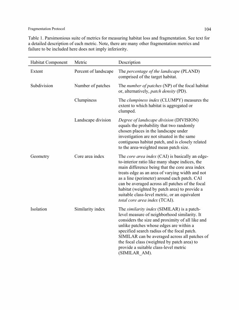
104Fragmentation Protocol
Table 1. Parsimonious suite of metrics for measuring habitat loss and fragmentation. See text fora detailed description of each metric. Note, there are many other fragmentation metrics andfailure to be included here does not imply inferiority.
Habitat Component Metric Description
Extent Percent of landscape The percentage of the landscape (PLAND)comprised of the target habitat.
Subdivision Number of patches The number of patches (NP) of the focal habitator, alternatively, patch density (PD).
Clumpiness The clumpiness index (CLUMPY) measures theextent to which habitat is aggregated orclumped.
Landscape division Degree of landscape division (DIVISION)equals the probability that two randomlychosen places in the landscape underinvestigation are not situated in the samecontiguous habitat patch, and is closely relatedto the area-weighted mean patch size.
Geometry Core area index The core area index (CAI) is basically an edge-to-interior ratio like many shape indices, themain difference being that the core area indextreats edge as an area of varying width and notas a line (perimeter) around each patch. CAIcan be averaged across all patches of the focalhabitat (weighted by patch area) to provide asuitable class-level metric, or an equivalenttotal core area index (TCAI).
Isolation Similarity index The similarity index (SIMILAR) is a patch-level measure of neighborhood similarity. Itconsiders the size and proximity of all like andunlike patches whose edges are within aspecified search radius of the focal patch.SIMILAR can be averaged across all patches ofthe focal class (weighted by patch area) toprovide a suitable class-level metric(SIMILAR_AM).

105Fragmentation Protocol
Connectedness Correlation length The correlation length index (CLI) is a measureof the structural continuity or connectedness ofthe focal habitat based on a measure of theextensiveness of each patch as measured by theradius of gyration (GYRATE). CLI isequivalent to the area-weighted mean radius ofgyration (GYRATE_AM).
Traversability The traversibility index (TRAVERSE) is afunctional measure of connectivity based on theidea of ecological resistance. This metric uses aresistance surface to determine the area that canbe reached from each cell in the focal habitat
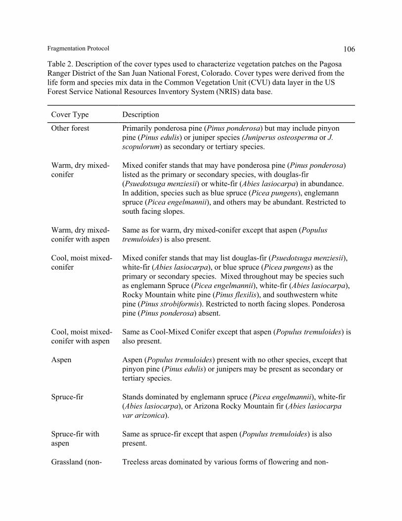
106Fragmentation Protocol
Table 2. Description of the cover types used to characterize vegetation patches on the PagosaRanger District of the San Juan National Forest, Colorado. Cover types were derived from thelife form and species mix data in the Common Vegetation Unit (CVU) data layer in the USForest Service National Resources Inventory System (NRIS) data base.
Cover Type Description
Other forest Primarily ponderosa pine (Pinus ponderosa) but may include pinyonpine (Pinus edulis) or juniper species (Juniperus osteosperma or J.scopulorum) as secondary or tertiary species.
Warm, dry mixed-conifer
Mixed conifer stands that may have ponderosa pine (Pinus ponderosa)listed as the primary or secondary species, with douglas-fir(Psuedotsuga menziesii) or white-fir (Abies lasiocarpa) in abundance. In addition, species such as blue spruce (Picea pungens), englemannspruce (Picea engelmannii), and others may be abundant. Restricted tosouth facing slopes.
Warm, dry mixed-conifer with aspen
Same as for warm, dry mixed-conifer except that aspen (Populustremuloides) is also present.
Cool, moist mixed-conifer
Mixed conifer stands that may list douglas-fir (Psuedotsuga menziesii),white-fir (Abies lasiocarpa), or blue spruce (Picea pungens) as theprimary or secondary species. Mixed throughout may be species suchas englemann Spruce (Picea engelmannii), white-fir (Abies lasiocarpa),Rocky Mountain white pine (Pinus flexilis), and southwestern whitepine (Pinus strobiformis). Restricted to north facing slopes. Ponderosapine (Pinus ponderosa) absent.
Cool, moist mixed-conifer with aspen
Same as Cool-Mixed Conifer except that aspen (Populus tremuloides) isalso present.
Aspen Aspen (Populus tremuloides) present with no other species, except thatpinyon pine (Pinus edulis) or junipers may be present as secondary ortertiary species.
Spruce-fir Stands dominated by englemann spruce (Picea engelmannii), white-fir(Abies lasiocarpa), or Arizona Rocky Mountain fir (Abies lasiocarpavar arizonica).
Spruce-fir withaspen
Same as spruce-fir except that aspen (Populus tremuloides) is alsopresent.
Grassland (non- Treeless areas dominated by various forms of flowering and non-

107Fragmentation Protocol
forest) flowering plant species, herbs, forbs, and legumes.
Riparian Areas dominated by hydrophilic plant and tree species.
Shrubland Lower elevation areas dominated by gamble oak (Quercus gambelii )and petran chaparral.
Bare rock Areas with bare rock such as boulder fields, cliff-faces, andoutcroppings.
Water All rivers, streams, ponds and reservoirs.

108Fragmentation Protocol
Table 3. Reclassification of original cover types used to characterize vegetation patches on thePagosa Ranger District of the San Juan National Forest, Colorado (see Table 2) into fouraggregate classes for the purpose of assessing fragmentation of late-seral coniferous forest.
Cover Type Description
Late-seral coniferousforest
Warm, dry mixed-conifer (with and without aspen); Cool, moistmixed-conifer (with and without aspen); and Spruce-fir forest(with and without aspen); all in the understory reinitiation orshifting mosaic, old-growth stage of stand development.
Mid-seral coniferousforest
Same cover types as above, but in the stem exclusion stage ofstand development.
Early-seral coniferousforest & Aspen
Same cover types as above, but in the stand initiation stage ofstand development, plus Aspen stands in any stage ofdevelopment.
Nonforested & lowelevation forest
All other cover types, including Other forest, Grassland, Riparian,Shrubland, Bare rock, and Water.

109Fragmentation Protocol
Table 4. Similarity coefficients used in the similarity index (SIMILAR) for the analysis of late-seral coniferous forest isolation. See text for a description of the similarity index and its use inthis exercise. Coefficient of 1 equals maximum similarity to the focal habitat - in this case, late-seral coniferous forest.
Focal cover type
Nonforested &low elevationforests
Early-seralconiferousforest & aspen
Mid-seralconiferousforest
Late-seralconiferousforest
Late-seral coniferousforest
0 0.1 0.3 1
110Fragmentation Protocol
FIGURE CAPTIONS
1. Schematic illustration of the patch versus landscape perspectives on habitat fragmentation.In the patch perspective, a patch can be reduced in size (area effect) or become more isolated(isolation effect) from nearby patches, but these effects are relative to a focal patch. In thelandscape perspective, a contiguous habitat distribution or suite of habitat patches can bereduced in areal extent (area effect) and subdivided into disjunct patches (fragmentationeffect), and these effects are relative to the entire landscape.
2. Schematic illustration of the island biogeographic versus landscape mosaic perspectives onhabitat fragmentation. In the island biogeographic perspective habitat fragments are viewedas analogues of oceanic islands in an inhospitable sea or ecologically neutral matrix. In thelandscape mosaic persepective, landscapes are viewed as spatially complex, heterogeneousassemblages of patches of differing types, which can’t be simplified into a dichotomy ofhabitat and matrix.
3. Idealized phases of the habitat loss and fragmentation process, beginning with (A) dissectionof the habitat (often by roads); followed by (B) perforation, usually associated with habitatconversion (e.g., development, timber harvest, etc.); ultimately resulting in (C) subdivisionof contiguous habitat into disjunct habitat fragments; and culminating in (D) shrinkage andattrition as habitat is reduce to scattered fragments or eventually eliminated altogether.
4. Idealized alternative models of habitat loss and fragmentation, including (A) habitat lost in arandom fashion, (B) habitat lost in a contagious (i.e., aggregated) manner, (C) habitat lost ina dispersed (i.e., disaggregated) pattern, (D) habitat lost progressively in a wave-like manneralong an edge, (E) habitat first bisected by corridor development (e.g., roads) and then lostprogressively outward from the corridors, and (F) habitat lost progressively from nuclei thatmay be dispersed in a random, uniform, or clumped pattern. In these examples, habitat isprogressively altered by disturbance over three time periods. Disturbed areas slowly recoverover time following disturbance, as in a dynamic forested landscape. Black represents theoriginal, unaltered habitat; white represents recently disturbed areas, and the two shades ofgray represent increasing stages of recovery following disturbance. Note, these models couldalso be represented by progressive loss and fragmentation of habitat without recoveryfollowing disturbance, as in a landscape undergoing transformation due to urban and/oragricultural development.
5. Alternative landscape definitions for an arbitrary area on the San Juan National Forest insouthwest Colorado. The island biogeographic perspective (see Fig. 2) depicts the focalhabitat against an ecologically neutral matrix, whereas the landscape mosaic perspective (seeFig. 2) depicts the focal habitat in a mosaic of other patch types. The focal habitat is definedat three levels of measurement resolution: (A-B) old-growth spruce-fir forest, (C-D) old-growth conifer forest, and (E-F) all forest.
111Fragmentation Protocol
6. Vector versus raster data models for an arbitrary landscape. In the vector model, patches arerepresented as polygons; whereas, in the raster model, patches are represented as contiguouslike-valued cells in a square grid lattice.
7. Effects of changing spatial grain from 25 m (high resolution) to 100 m (low resolution) onfour representative landscape metrics for an arbitrary landscape: (1) Simpson’s diversity, ameasure of overall landscape diversity reflecting the variety and relative abundance of patchtypes; (2) contagion, a measure of overall clumpiness of patch types, (3) patch density, asimple measure of the number of patches per unit area, and (4) edge density, a simplemeasure of the length of edges between patches per unit area.
8. Effects of changing spatial extent from a relatively small landscape to a relatively largelandscape on four representative landscape metrics (see figure 7 caption for a description) foran arbitrary landscape.
9. Boundary effects vary as a function of the internal heterogeneity of the landscape. Inrelatively fine-grained landscapes, the boundary of the landscape represents proportionatelyless of the total edge and therefore has less effect (bias) on the computed value of the metric.In relatively coarse-grained landscapes, however, the boundary of the landscape has aproportionately greater effect.
10. Landscape spatial context (i.e., the broader regional context) of the project area has animportant impact on the biological consequences of habitat loss and fragmentation at thelocal landscape scale. For example, areas of highly fragmented habitat (shown in dark)within a matrix of continuous habitat may not suffer adverse fragmentation effects due to thebuffering effect of the broader habitat matrix; whereas, areas of unfragmented habitat withina highly fragmented matrix may suffer significant fragmentation effects for the oppositereasons.
11. Trajectories of change in habitat extent (PLAND) and configuration (represented here by theclumpiness index, CLUMPY) for late-seral coniferous forest habitat (A-B) and pine martenhabitat (C-D) under a simulated wildfire disturbance regime representing an historicreference period on the San Juan National Forest in southwest Colorado. These trajectoriesillustrate the dynamic nature of habitat resulting from the interplay between disturbance andsuccession processes.
12. Arbitrary landscapes illustrating differences in habitat (shown in dark) extent, as measuredby the percentage of the landscape (PLAND). Habitat is illustrated here using an islandbiogeographic model (see Fig. 2) of landscape structure for simplicity.
13. Arbitrary landscapes illustrating differences in habitat (shown in dark) subdivision, asmeasured by the number of patches (NP), clumpiness index (CLUMPY) and landscapedivision index (DIVISION). Habitat is illustrated here using an island biogeographic model(see Fig. 2) of landscape structure for simplicity. Habitat extent (PLAND) is held constantamong landscapes to highlight the independent effect of habitat subdivision.
112Fragmentation Protocol
14. Arbitrary landscapes illustrating differences in habitat (shown in dark) geometry, asmeasured by the total core area index (TCAI). Habitat is illustrated here using an islandbiogeographic model (see Fig. 2) of landscape structure for simplicity. Habitat extent(PLAND) is held constant among landscapes to highlight the independent effect of habitatsubdivision.
15. Arbitrary landscapes illustrating differences in habitat (shown in dark) isolation, as measuredby the similarity index (SIMILAR_AM) based on an arbitrary search radius and logicalsimilarity coefficients. Focal habitat extent (PLAND) is held constant among landscapeswhile the overall landscape composition and configuration varies to highlight theindependent effect of habitat isolation.
16. Arbitrary landscapes illustrating differences in the structural or physical continuity (i.e.,connectedness) of habitat (shown in dark) as measured by the correlation length index (CLI;also referred to as the area-weighted mean patch radius of gyration, GYRATE_AM). Habitatis illustrated here using an island biogeographic model (see Fig. 2) of landscape structure forsimplicity. Habitat extent (PLAND) is held constant among landscapes to highlight theindependent effect of habitat connectedness.
17. Arbitrary landscapes illustrating differences in the functional connectivity (i.e.,connectedness) of two locations as measured by the traversability index (TRAVERSE). Thelandscape are illustrated here using a landscape mosaic model of landscape structure whereeach land cover type is assigned a different level of resistence (e.g., corresponding to thedifficulty of the focal organism(s) successfully traversing a unit length of that cover type, sayduring dispersal) relative to the focal cover type (shown in gold). The least cost hull (i.e., themaximum traversable area) is depicted by the solid dark line, with contours spreadingoutward from the focal cell. The traversability value shown is for the corresponding focalcell; however, the traversability index (not shown) is computed as the average traversabilityacross all cells of the focal habitat.
18. Outline of the major steps in the habitat loss and fragmentation assessment protocol.
19. Project area location on the Pagosa Ranger District of the San Juan National Forest insouthwestern Colorado, U.S.A. The project area comprises the 40,000 ha Piedra Riverwatershed.
20. Land cover map of the project area on the Pagosa Ranger District of the San Juan NationalForest in southwestern Colorado, U.S.A. Land cover types represent combinations of themajor vegetation types and seral stages of forest stand development (see Table 2 for adescription of each cover type).
21. Reclassified land cover map of the project area on the Pagosa Ranger District of the San JuanNational Forest in southwestern Colorado, U.S.A. All high-elevation coniferous forest types(spruce-fir, cool-moist mixed-conifer, and warm-dry mixed-conifer, each with and without

113Fragmentation Protocol
aspen) in the understory reinitiation and old-growth, shifting mosaic seral stages werecombined into a single “late-seral coniferous forest” class (see Table 3 for details). Map onleft shows the original land cover map (as in Fig. 20) and the map on the right is thereclassified landscape.
22. Pine marten habitat capability map for the project area on the Pagosa Ranger District of theSan Juan National Forest, Colorado. The map represents one snapshot of habitat conditionsduring a 600-year landscape simulation under the wildfire scenario (see text for details).Black represents habitat and the various shades of grey represent non-habitat.
23. Late-seral coniferous forest habitat trajectories of change over 200-300 years under fourtimber harvest scenarios: (1) long-rotation (300 yrs), aggregated cutting pattern; (2) long-rotation, dispersed cutting pattern; (3) short-rotation (200 yrs), aggregated cutting pattern;and (4) short-rotation, dispersed cutting pattern (see text for details). The mean and 90%range of variation (5-95th percentile) under the reference conditions, simulated here as awildfire scenario, is shown in the dashed (mean) and solid light lines. Sub-figures representdifferent landscape metrics: (A) percentage of the landscape, PLAND; (B) number ofpatches, NP; (C) clumpiness index, CLUMPY; (D) landscape division index, DIVISION; (E)total core area index, TCAI; (F) similarity index, SIMILAR_AM; and (G) correlation length,or the area-weighted mean patch radius of gyration, GYRATE_AM (see Table 1 fordescriptions of metrics).
24. Pine marten habitat trajectories of change over 200-300 years under four timber harvestscenarios (see figure 23) and the mean and 90% range of variation (5-95th percentile) underthe reference conditions, simulated here as a wildfire scenario, is shown in the dashed (mean)and light lines. Pine marten habitat was defined as cells with habitat capability values > 0.7computed from a habitat capability model. Subfigures represent different landscape metrics:(A) percentage of the landscape, PLAND; (B) number of patches, NP; (C) clumpiness index,CLUMPY; (D) landscape division index, DIVISION; (E) total core area index, TCAI; (F)similarity index, SIMILAR_AM; and (G) correlation length, or the area-weighted meanpatch radius of gyration, GYRATE_AM.