Quantitative Analysis of Immigrants

Self-Selection and its Implications

Joel Lopez Real

Department of Economics Universidad Carlos III, 28093 Getafe Madrid, SPAIN

Abstract

How is affected the investment in human capital by the possibility of future migra-tion? Who is actually migrating? And, what is the effect of international migrationin differences in output p.c. across countries? I present a model with heterogeneousagents that decide endogenously investment in human capital and migration. I findthat the possibility of migration induce to overinvest in human capital. I concludethat the migration pattern of self-selection is not unique. Finally, I test if the modelcan replicate migration patterns for three different cases: Mexico, India and UK toUS. I match the data in average years of schooling for immigrants and natives andrelative earnings of immigrants with respect to US born-natives.

Key words:PACS:

Email address: jlreal@eco.uc3m.es (Joel Lopez Real).URL: http://www.eco.uc3m.es/jlreal/ (Joel Lopez Real).

Preprint submitted to Elsevier 31 October 2008

1 Introduction

How is affected the investment in human capital by the possibility of futuremigration? Who is actually migrating? And, what is the effect of internationalmigration in differences in output p.c. across countries? I present a modelwith heterogeneous agents that decide endogenously investment in humancapital and migration. This original approach permits me to answer thesequestion linking two literatures, migration and economic growth. Moreover,if the accumulation of human capital is affected by the possibility of futuremigration, then there is no sense in study separately these questions as hasbeen made in previous works.

Are immigrants positive or negative self-selected? This is a traditional questionin migration literature. It is important because the effects of international mi-gration depend crucially on the pattern of immigrants. Although the migrationliterature has focus mostly on the effects of immigrants in the hosting country,international migration has effects is the source country too. The brain draintheory stresses this idea and suggests that the migration of population thatis relatively high skill has negative effects in the source country. At this pointthere is controversy too. If people become more educated because they knowthat in the future they will migrate may be the case that the brain drain haspositive effects. This is called the induced education effect. Obviously, to testall these ideas we need a model where accumulation of human capital andmigration decision are endogenous, otherwise it is impossible. Finally, once weknow who is migrating and what determine the pattern of immigrants, we canquantify the effects in differences in output per capita across countries and tryto test different migration policies.

The main particularities of the model are: (i) It is an international modelwith two economies and perfect physical capital mobility. (ii) There are OGof dynasties composed by households. (iii) Households are heterogeneous anddecide consumption, physical capital investment, human capital investmentand migration. (iv) Human capital is produced using two inputs, time andexpenditure in goods. (v) Migration is costly. I will consider two types ofcosts. A fix migration cost that can be interpreted as travel expenses and atime migration cost. For the moment think in the time migration cost as allthe time that you need to prepare the migration. This cost affects the effectiveunits of labor.

I find that optimal investment in human capital of immigrants is clearly abovethe investment in human capital in a closed economy most of the cases. Thissupports the thesis of induce education effect of brain drain theory. The sig-nificance of the induce education effect depends on the relative size of themigration costs, the TFP of and the migration rate. Related with this I find

2

that the migration pattern of self-selection is not unique. For the same migra-tion costs Immigrants are positive self-selected for higher TFP countries whilethey are negative self-selected for lower TFP countries. To increase the timecost, all the rest constant, decreases the migration rate and implies higherpositive self-selection. I have tested the model for the case of Mexico, Indiaand UK. These three cases present so many different particularities amongthem that are good candidates to test the model in different dimensions. Ifind that the model can replicate real selection patterns of immigrants for ac-ceptable parameter values. I find that average years of Mexican immigrantsis 7.2 and Mexican natives is 5.1 Data for Mexican immigrants is 7.5 and 6.3for natives. For the Indian case I find a strong positive self-selection as dataindicates. I find that average years of schooling is 12.88 for immigrants and4 for natives. Data for Indian immigrants is 15.6 and 5 for natives. I also getthat immigrants from UK earns more than US native. I find a earnings ratioof 1.2 when real ratio is 1.3. Average years of schooling of immigrants fromUK is 14.8 and in data it is 14.6.

Borjas has been the pioneer in the migration literature. He tried to answerthe self-selection question using a simple partial static model derived fromthe Roy’s model. In Borjas (1994) he finds that immigrants are positive self-selected when correlation of skills is sufficiently high and distribution of earn-ings is higher in the hosting country. But if the source country has higherearnings dispersion than the hosting country then immigrants are negative self-selected. It is well?*** to point out that Borjas defines positive self-selectionas having above average earnings in both the source and the host countryand in an equivalent way for negative self-selection. When I talk of positiveself-selection I mean that the average level of human capital of immigrantsis higher than those in the source country. Independently of whether theywill finish in the distribution of skills in the host country. Since US disper-sion of earnings distribution is lower than dispersion of earnings distributionin developing countries, Borjas’ model supports the thesis of negative self-selection. But if we take I look to data, there is a high brain drain in theCaribbean, some Africa countries and India and the dispersion of earningsin these economies are higher than in US. Stark (1994) defends that in caseof asymmetric information it is possible to have negative self-selection sinceemployers can not know the type of the immigrant. Other statical models areChiswick (1999) and (2000) and Belletini and Berti (2006). Chiswick findspositive self-selection adding in his theoretical model a migration cost that isless important the more skill is the immigrant. Belletini and Berti find that thelower is the wage level in the hosting country the higher is the percentage ofskilled people among the immigrants. In all these works there is no investmentin human capital and migration decision. They perform a statical comparisonof earnings in both countries and study under which conditions earnings arehigher in the foreign country. They are very far from what I am doing here.

3

In the closest work to mine, Urrutia (2001) analyzes in a dynastic OG modelthe effect of migration costs on the self-selection of immigrants. In his modelthere are two migration costs. A fix cost and a loss of ability. He finds thatwhen the fixed cost is relatively low, immigrants are selected from the bottomof the distribution of abilities while if the fix cost is relatively high then theopposite happens. Although he finds different selection patterns dependingon the relative size of the costs, in his model the ability is exogenous so hecan not explain the relationship between investment in human capital andmigration. And this relationship may be affecting the self-selection of immi-grants. Moreover he abstracts the results from real differences in TFP acrosscountries.

Others papers where emigration is endogenous are Klein and Ventura (2006)and (2007). They are interested in studding an efficient reallocation of laborin the world. In these papers agents are endowed with birthplace dependentefficiency units of labor so, again there is no accumulation of human capital.

There is a long debate on why differences in output per capita are so big acrosscountries. Mankiw, Romer and Weil (1992) used an augmented Solow modeland estimated that output differences were caused by human capital differ-ences. On the contrary Klenow and Rodriguez-Clare (1997), Hall and Jones(1999), Bils and Klenow (2000) and Parente and Prescott (2000) support thatdifferences in output per capita are due to differences in TFP. The most recentwork is Hendricks (2002) who estimates human capital of different countriesfrom immigrants in the US job market doing the same work and supportsthe TFP thesis. For the production function of human capital I will followSeshadri and Manuelli (2007) [hereafter M-S] and, mainly Erosa, Koreshkova,and Restuccia (2007) [hereafter E-K-R]. These authors stresses the idea of theimportance of education quality. Once they take into account that educationquality may differ among countries they conclude that relatively small differ-ences in TFP levels accounts for big output differences across countries. Thecommon problem in the human capital theory is that it does not take intoaccount migration. But if we are concerned about importance of human cap-ital in international accounting we must be worried about migration becausemigration is nothing else that mobility of human capital across countries.

The paper is organized as follows. Section 1 describes the model. In section 2I show the calibration of the parameters, the targets and values and I presentthe benchmark economy. In section 3 I present the results for a closed econ-omy, for an open economy with fix migration cost and for an open economywith both migration costs. In section 4 I use the model two mach two realcases, immigrants from Mexico and India to US. The effect of immigrantsin differences in output per capita across countries are showed in section 5.Section 6 concludes.

4

2 The Model

Since I will consider the steady state equilibrium I use the usual conventionof denote by primes next period variables.

2.1 Locations

There are two economies that I identify with the index i ∈ {0, 1}. I interpreteconomy indexed by 0 as a developing country and economy indexed by 1as a developed country. As it is usual in international economics literatureI will refer to country 0 as the South economy and country 1 as the Northeconomy. Locations only differ in two features, their level of TFP and theirnatural population growth rates. I will be more precise in how they differ inthe following sections. Finally, physical capital is perfect mobile in the worldeconomy.

2.2 Technologies

There are two technologies. One for goods and another for human capital.Output is produced in each economy according to the the technology

Yi = AiKαi H

1−αi for i ∈ {0, 1}

where Yi is output and Ki and Hi are aggregated physical capital and aggre-gated human capital respectively in economy i 1 .I make the assumption thatthe north economy is more productive than the south economy, A1 > A0.

I follow E-K-R to model the production function of human capital. Per capitahuman capital is produced with two inputs, time s ∈ [0, 1] and expenditure ingoods allocated to education e and takes the form:

h′

= z′(sηe1−η)ξ η, ξ ∈ (0, 1)

where z′is a stochastic shock that refers to the individual ability to accumulate

human capital.

1 Note that factor shares are equal in both economies. Gollin (2002) supports theassumption that labor shares are equal in both economies

5

2.3 Demographic Structure

Each economy is modelled as an OG of dynasties that are altruistic towardthe dynasty. There are a large number of dynasties that are composed byhouseholds. In a household there are two types of agents. Agents live twoperiods. In the first period they are young agents and in the second periodthey are old agents. Young agents live in the household with an old agent andwhen they become old a new household is realized. So, in a household thereis always an old agent and young agents.

Old agents take all the decisions inside the household in a sense that I willbe more precise shortly. But in order to understand dynamics of the popula-tion consider that an old agent decides where their descendants start a newhousehold 2 . Then, using in advance the result that migration pattern is fromeconomy 0 to economy 1 (south to north) I can write population dynamics ineach economy as:

N′

1 = (1 + n1)N1 +m(1 + n0)N0 (1)

N′

0 = (1 + n0)(1−m)N0 (2)

where Ni is total population and ni denotes natural population growth rate incountry i. I assume that natural population growth rate is higher in country0 (see appendix for a full description of population dynamics and its im-plications). Since migration is unidirectional m stands for the proportion ofhouseholds in country 0 that decide to leave the native country and establishin country 1 3 .

2.4 Preferences and Endowments

The household gets utility from consumption. The utility function takes theform:

u(c) =c1−γ

1− γ

2 It means that old agents take the migration decision for their descendants. Thealternative that young agents decide if migrate does not change results but compu-tationally is costlier3 Since the number of young agents per household is constant and equal for all thedynasties the proportion of households that migrate is the same that the proportionof population migrating

6

Young agents receive an idiosyncratic shock to their ability z ∈ Z = {z1, ..., zn}and it is an unobservable for old agents. This shock follows a markovian processwith transition matrix πz,z′ . This shock is the same for all the members of thehousehold. Moreover, is the same process in both countries.

2.5 The Household’s Problem

In a household there are two types of agents, the young agent and the oldagent. In the second period of their life young agents become old agents andstart a new household as an old agent. Old agents take all the decisions insidethe household and they are altruistic toward their descendants. An old agentdecide per capita consumption c and per capita assets for the next perioda

′. Note that a

′will be the bequest for the next generation. Furthermore,

they decide how much time and expenditure in goods must be allocated inthe human capital production function of their children. Finally, old agentsdecide where their descendants are going to start the new household. If theytake the migration decision all their descendants migrate and start abroadthe next period. For the moment I will assume that if they migrate they onlyhave to pay a fix migration cost θ. I interpret this cost as travel expenses. Theliterature always relates this cost with the distance from the source countryto the host country. For instance, Urrutia defines this cost as travel expensesand the cost of keep in contact with the native country.

The household gets income from old agent earnings, from young agents earn-ings and from assets. Note that young agents earnings depend on the remainingtime after investment in education and also depends on ψ. This parameter is tocontrol for the life cycle profile of wages. I have normalized to 1 this parameterfor old agents.

The problem faced by a household in country 1 taking into account that theydo not migrate is:

V (a, h, z, 1) = maxc,e,s,a′

{u(c) + β(1 + n1)∑z′πz,z′V (a

′, h

′, z

′, 1)}

c+ (1 + n1)e+ (1 + n1)a′ ≤w1h+ (1 + n1)(1− s)w1ψ +Ra

h′= z

′(sηe1−η)ξ

a′, e≥ 0, s ∈ [0, 1]

The problem faced by a household in country 0 is very similar but presentsthe particularity that households decide whether to start the next period. Ifthey migrate then i

′= 1 and they have to pay θ. The problem is:

7

V (a, h, z, 0) = maxc,e,s,a′ ,i′

{u(c) + β(1 + n0)∑z′πz,z′V (a

′, h

′, z

′, i

′)}

c+ (1 + n0)e+ (1 + n0)a′ ≤w0h+ (1 + n0)(1− s)w0ψ +Ra− i′θh

′= z

′(sηe1−η)ξ

i′= {0, 1}, a

′, e ≥ 0, s ∈ [0, 1]

3 Calibration

3.1 Parameters and Targets

The calibration strategy takes two steps. First, I calibrate the benchmark econ-omy to join US data in a closed economy. Second, I calibrate the open economywith migration. The open economy requires additional parameters values asfor instance south natural population growth rate and the fix migration cost.For the moment I will focus on the calibration of the closed economy.

The length of a period is 30 years. I model the life of an agent from age 6 to age66. I start modelling from age 6 to capture better human capital investmentdecision and it is a common strategy in human capital literature. Age 66 isroughly retirement age. I normalize TFP of country 1 equal to 1 (A1 = 1).In US the natural population growth rate n1 is 0.59% and population growthrate np1 is 0.92% 4 . I set δ = 0.0668 and α = 0.33 from Cooley and Prescott(). The coefficient of the CRRA utility function σ is set equal to 2, which is inthe range of usually accepted values in this literature 5 . I calibrate β to matchan annual interest rate of 5%. I sum up the parameters and their values intable (#)

Parameter Value

TFP A1 1

US natural population growth rate n1 0.59%

US population growth rate np1 0.92%

Discount Factor β 0.945

CRRA σ 2

Physical capital share α 0.33

Physical capital depreciation δ 0.07

4 U.S. Census Bureau, International Data Base, year 20055 See for instance Keane and Wolpin (2001), Klein and Ventura (2007) and E-K-R

8

It remains to choose the parameters related to the human capital investment.These parameters are: η,ξ,ψ and the shock z for the ability. I calibrate theshock z as in E-K-R where ability follows in logs an AR(1) process 6 . I use5 shocks to approximate this process with a Markov chain. To calibrate theshocks I use the procedure in Tauchen (1986). This process implies 2 additionalparameters values ρz and σ2

z . Then, I have to calibrate 5 parameter values. Todo this I use U.S. cross-sectional data. The targets are:

(1) M-S take average years of education equal to 12.08 from Barro and Lee(1996). In E-K-R average years of education are 12.9 from U.S. Depart-ment of Education 2004.

(2) Intergenerational correlation of log-earnings of 0.5 from Mulligan (1997).

(3) Variance of log-earnings of 0.36 from Mulligan (1997).

(4) Mincer returns to schooling of 10% in average.

(5) Percentage of people with college education or higher equal to 54%. Itmeans that percentage of people with less than college (Elementary andHigh School) is 46%.

The process of matching each parameter with its target is quite complicated. Ihave run several experiments to arrive to the following conclusions. Intergen-erational correlation of log-earnings is mainly affected by ρz and variance oflog-earnings depends mainly on σ2

z . I relate ψ with average years of schoolingbecause the main effect of this parameter is that it moves all the distribution(primary, secondary and college) to the right or to the left. Mincer returns andpercentage of people with college or higher are related because the less peopleare with college the higher the mincer returns are. But, Mincer returns aremore sensitive to variations in ξ and η affects more the percentage of peoplewith college. In table (#) I link each parameter with its target and its valuein the calibrated model.

6 AR(1) process for ability in logs takes the form :

log(z′) = ρzlog(z) + εz where εz ∼ N(0, σ2

z)

9

Target Parameter Value

% of people with college η 0.76

Mincer returns ξ 0.55

Average years of schooling ψ 0.06

Variance of log-earnings σ2z 0.46

Intergenerational correlation of log-earnings ρz 0.13

3.2 The Benchmark Economy

Table (#) presents the US data targets and the benchmark economy.

Target US data BE

Average years of education 12.9 12

Intergenerational correlation of log-earnings 0.5 0.5

Variance of log-earnings 0.36 0.35

Mincer returns to schooling of 10% 7.7%

Percentage of people with college education or higher 54% 55%

The benchmark economy replicates quite well the targets, even though I amunderestimating mincer returns. Although it is not obvious how to relate realdata on Mincer returns with data from the model since the length of theperiods are quite different. I have calculated some others facts for which themodel has not been calibrated. For instance, the ratios of total median earningsfor different levels of highest education attainment. These ratios are:

US data BE

Primary/Secondary 0.65 0.57

Secondary/Secondary 1 1.

College/Secondary 1.86 1. 83

I am doing quite well in the ratio of college with secondary and I am underesti-mating the ratio primary with secondary. Of course there is always a problemwhen we try to link this real data with data from the model where investmentin time is continuous. If I do an interval taking as a lower bound the value forsome degree of completion and as an upper bound full completion, then myresults fall in this interval.

10

As a measure of inequality I have computed the Gini index for the benchmarkeconomy. The US Gini index is 0.611 for earnings from 1998 Survey of Con-sumer Finances and I get a Gini index of 0.70. It does not seem that the modeldoes a good job to explain inequality, maybe a solution would be to increasethe number of shocks. I have compute expenditures in education. Havemanand Wolfe (1995) reports that total expenditures in children from 0 to 18 are14.5% of GDP. They also report that expenditures on elementary, secondaryand post-secondary schooling are 6.6% of GNP (U.S. Bureau of the Census1992). E-K-R get a ratio of 12% that is close to Haveman and Wolfe’s resultwhen foregone parental earning are subtracted. M-S use as a target that ex-penditures in schooling as a fraction of GDP is 3.77% from OECD. The dataI found suggests an upper bound of 6.6% from the OECD for 2004. I get inthe benchmark economy a expenditure ratio of 2.12% which is lower.

4 Results

4.1 Closed Economy

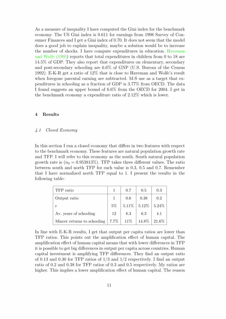
In this section I run a closed economy that differs in two features with respectto the benchmark economy. These features are natural population growth rateand TFP. I will refer to this economy as the south. South natural populationgrowth rate is (n0 = 0.953813%). TFP takes three different values. The ratiobetween south and north TFP for each value is 0.3, 0.5 and 0.7. Rememberthat I have normalized north TFP equal to 1. I present the results in thefollowing table:

TFP ratio 1 0.7 0.5 0.3

Output ratio 1 0.6 0.38 0.2

r 5% 5.11% 5.12% 5.24%

Av. years of schooling 12 8.3 6.3 4.1

Mincer returns to schooling 7.7% 11% 14.8% 21.6%

In line with E-K-R results, I get that output per capita ratios are lower thanTFP ratios. This points out the amplification effect of human capital. Theamplification effect of human capital means that with lower differences in TFPit is possible to get big differences in output per capita across countries. Humancapital investment is amplifying TFP differences. They find an output ratioof 0.13 and 0.30 for TFP ratios of 1/3 and 1/2 respectively. I find an outputratio of 0.2 and 0.38 for TFP ratios of 0.3 and 0.5 respectively. My ratios arehigher. This implies a lower amplification effect of human capital. The reason

11

is that in E-K-R’s model the time that an agent invests in human capitalaccumulation is costly too. It makes the amplification effect higher. Averageyears of schooling are in concordance with previous works. For instance, M-Sreport that for output per worker ratio to US of 0.244 the average is 5.18 and5.88 for an output per worker ratio of 0.354. For output ratios of 0.5 and 0.7the average falls in the intervals (7.54-8.12) and (8.7-9.72) respectively. E-K-Rfind an average of 4.3 for a TFP ratio of 1/3 and an average of 7.1 for a TFPratio of 1/2. Mincer returns decreases with higher average years of education.I obtain Mincer returns of 11%, 14.8% and 21.6% for TFP ratios of 0.7, 0.5and 0.3. E-K-R get results very similar. They estimate Mincer returns of 14.5and 22.6 for TFP ratios of 1/2 and 1/3. Finally, I report endogenous interestrate. Remember that the benchmark economy has been calibrated to matchan interest rate of 5%. Then, for lower TFP values, the interest rate increases.

4.2 Open Economy with fix migration cost

Equation (5) must hold in a open economy with migration in the steady stateequilibrium . This equation relates natural population growth rates and migra-tion in order to keep constant north and south ratios over the world populationor, equivalently, to equalize population growth rates in both economies. Thereare two different approaches to proceed. Either, I fix south natural populationgrowth rate and this implies a ratio of immigrants, or I fix as a target theratio of immigrants and this implies a south natural population growth rate.I have decided to fix a target of 1% of immigrants. Since the model period is30 years, it means broadly 0.033% of immigrants per year. The south naturalpopulation growth rate implied by this target is n0 = 0.953813%. To under-stand the magnitude of these numbers take as example data from Mexico.Mexico presents the biggest rate of migration to US and it is 0.15% per yearand Mexico natural population growth rate is 1.6% (from US Census Bureau,2005).

Once I have fixed the migration target, I proceed in the following way. Icalibrate the fix cost for a TFP ratio of 0.5 that gives 1% of immigrants. Themigration cost is calibrated as a fraction of average annual earnings in thebenchmark economy. This means that I define the fix cost as θw1 where w1

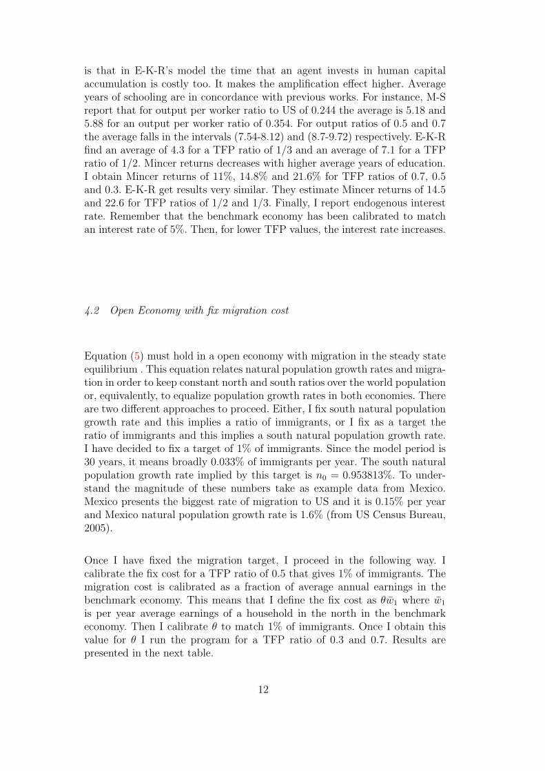
is per year average earnings of a household in the north in the benchmarkeconomy. Then I calibrate θ to match 1% of immigrants. Once I obtain thisvalue for θ I run the program for a TFP ratio of 0.3 and 0.7. Results arepresented in the next table.

12

TFP ratio 0.7 0.5 0.3

r 5% 5.6% 5.36%

Immigrants 8.7% 1% 0.22%

South av. years of schooling 4.8 3.5 3.6

Immigrants av. years of schooling 9 5.9 4.3

φ1 0.8 0.1 0.02

θ 3 3 3

Results suggest that immigrants are positive self-selected because averageyears of schooling of the immigrants are higher than those who do not em-igrate. Anyway, this result is sensitive to the size of the fix cost. There is afix cost size for which this result reverses and average years of education ofimmigrants are lower. Obviously, this effect is more important the lower isthe TFP ratio of a country because the cost is relatively more important. Ahousehold pays the fix migration cost and then invests in human capital. Ifthe cost is low, the household has resources to invest in human capital and canovertake human capital investment of those who do not migrate. But, if thecost is sufficiently high, then, when immigrants pay the fix migration cost thequantity of resources available is not enough to overtake investment of nativehouseholds. Imagine that I would have chosen the country with a TFP ratioof 0.3 to calibrate the fix migration cost that gives 1% of immigrants. In thatcase θ = 1.5 and immigrants average years of education is 1.6 while for southnatives is 2.6. So, there is negative self-selection but for a country with TFPratio of 0.5 the selection is positive.

Then, the model with fix migration cost has three main implications. First,for two countries with the same fix migration cost and different TFP level, theimmigrants from the country with higher TFP have higher average years ofschooling and, are more probably positive self-selected. Second, for two coun-tries with the same TFP level and different emigration cost, the immigrantsfrom the country with higher emigration cost are less educated and, are moreprobably negative self-selected. Third, for a country with TFP ratio of 0.7we observe that average years of education are 9. The same country but in aclosed economy has 8.2 average years of education. Then, there is the induceeducation effect that makes the south invest more in human capital whenmigration is possible. This effect is much stronger in next section.

Anyway, this model does not do a good job simulating migration pattern indifferent dimensions. There are two main limitations. The first problem withthe fix migration cost is that once a household can afford to pay the cost, thehousehold migrates. Since the fix cost is relatively less important for countrieswith higher TFP, the model implies higher migration ratios for countries with

13

higher TFP. The second problem is related. I am studying the steady stateequilibrium. In the steady state equilibrium can not be any household in thesouth that can pay the fix cost. They have migrated in a theoretical transition.This is the reason why average years of schooling in the south are lower withrespect to a closed economy.

4.3 Open Economy with two types of migration costs

To make the model more realistic I add another migration cost in line withmigration literature. Now, in addition to the fix migration cost, the householdswho decide to migrate experiment a loss in his effective labor hours. Thiscost can be interpreted as the time that a household expends making all thepreparatives to leave the native country, for instance: to look for a visa, tolook for a job in the hosting country, to cancel contracts in the native country,to sell and buy the house, etc. Moreover, the migration literature always usesa cost that represents a percentage of losses of earnings in the hosting countrydue for example to idiomatic difficulties. In some sense you can see this twoways of modelling as equivalent in my model but with the great advantagethat which I am using here is much easier to compute.

Introducing these two migration cost in the model the household’s problem inthe south becomes:

V (a, h, z, 0) = maxc,e,s,a′ ,i′

{u(c) + β(1 + n0)∑z′πz,z′V (a

′, h

′, z

′, i

′)}

c+ (1 + n0)e+ (1 + n0)a′ ≤w0h+ (1 + n0)(1− s)w0ψ +Ra− i′(θf + θvw0h)

h′= z

′(sηe1−η)ξ

i′= {0, 1}, a

′, e ≥ 0, s ∈ [0, 1]

The calibration of θf and θv has to be made very carefully. For the moment,just to understand the trade off between these two costs I am going to choosethe fix cost as 1/3 of the previous section and I will calibrate θv following theprevious procedure. It means that I will find the θv that gives 1% of immigrantsin the country with TFP ratio of 0.5. The effect of each migration cost andits calibration is crucial in the results. Although the calibration that I amusing here is arbitrary, for the moment it is enough to stress the role of themigration costs in the model. The trade off between both costs is illustrated inthe following graphics. These are the migration policy functions for differentTFP ratios and initial shock. Each line leaves to the left the households thatdo not migrate and to the right those that migrate.

When the unique migration cost considered was the fix migration cost, the

14

migration decision was an increasing function in the resources of the household.Resources of the household are income from assets and wages. It means thatonce the households can afford the fix migration cost, they decide to migrate.When the time cost is added, the migration decision is not always an increasingfunction in the initial level of human capital as before. A household with lowinitial level of human capital will be willing to migrate. The same householdwith more initial human capital will migrate even before since can pay easilythe fix migration cost. This is because the fix migration cost is relatively moreimportant than the time cost. But there is an initial level of human capitalwhere if I increase the initial level of human capital of a household and Ifix the same physical capital level, then the household that before decided tomigrate, now decides not to migrate. This is because at this point the time costis relatively more important than the fix migration cost. To sum up. When thefix cost is relatively more important than the time cost, then, more householdswill migrate for higher initial levels of human capital. When the time cost isrelatively more important that the fix migration cost, then, less householdswill migrate for higher initial levels of human capital. Finally, these graphicsshow that for a country with a TFP ratio of 0.3 the fix cost is relatively moreimportant and for a country with a TFP ratio of 0.7 the time cost dominatesthe fix migration cost. We can see exactly this mechanism in a country withTFP ratio of 0.5. For this country and low initial shock, the fix cost dominatesthe time cost but for higher initial shock the time cost starts to be present.

I repeat the same exercise that in the previous section and the results are

TFP ratio 0.7 0.5 0.3

r 5,64% 5.43% 5.51%

Immigrants 2.3% 1% 0.47%

South av. years of schooling 8.42 5.45 3.3

Immigrants av. years of schooling 22 13.72 2

φ1 0.22 0.097 0.058

θv 0.29 0.29 0.29

For countries with low TFP immigrants are negative self-selected and for coun-tries with high TFP immigrants are positive self-selected. The reason is thatfor low TFP countries the fix emigration cost is relatively more importantthat the time cost. There are two reasons that explain this. First, since theTFP is lower, the fix cost is relatively higher compared with a richer countrysuffering the same fix cost. Second, the investment in human capital in a poorcountry is lower, then, the time cost is also lower. For countries with higherTFP the time cost is relatively more important. This result is very crucial.Immigrants from higher TFP countries are positive self-selected but, further-

15

more, they are overinvesting in human capital with respect a situation with nomigration. Since the households know that if they migrate they suffer a loss intheir effective units of labor, they overinvest in human capital to compensatethis cost. Although the average years of schooling for an immigrant from acountry with TFP ratio equal to 0.7 is too high, these results give support tothe thesis of the induce education effect.

Moreover, although the number of immigrants increases with the TFP of thenative country, this effect is less important than in the previous section. Canbe the case for which immigrants decrease with the TFP level dependingon the calibration of the costs. Finally, interest rate may be higher in theopen economy with TFP ratio of 0.7 compared to the case of 0.3 due to theoverinvesting in human capital.

5 Mexico, India and UK cases

In this section I will test if the model can replicate two particular cases, im-migrants from Mexico, India and UK to US. Chiquiar and Hanson (2006)estimates that “Mexican immigrants, while much less educated than U.S. na-tives, are on average more educated than residents of Mexico” . Hendricksreports that average years of schooling of immigrants from Mexico to US is7.5 while average years of schooling of Mexican natives is 6.3. This implies aweak positive self-selection. For India he finds that immigrants have 15.6 yearsof education but natives have 5. This suggest a strong positive self-selection.Mexico and India differ in their TFP, in their migration rates to US and indistance to US.

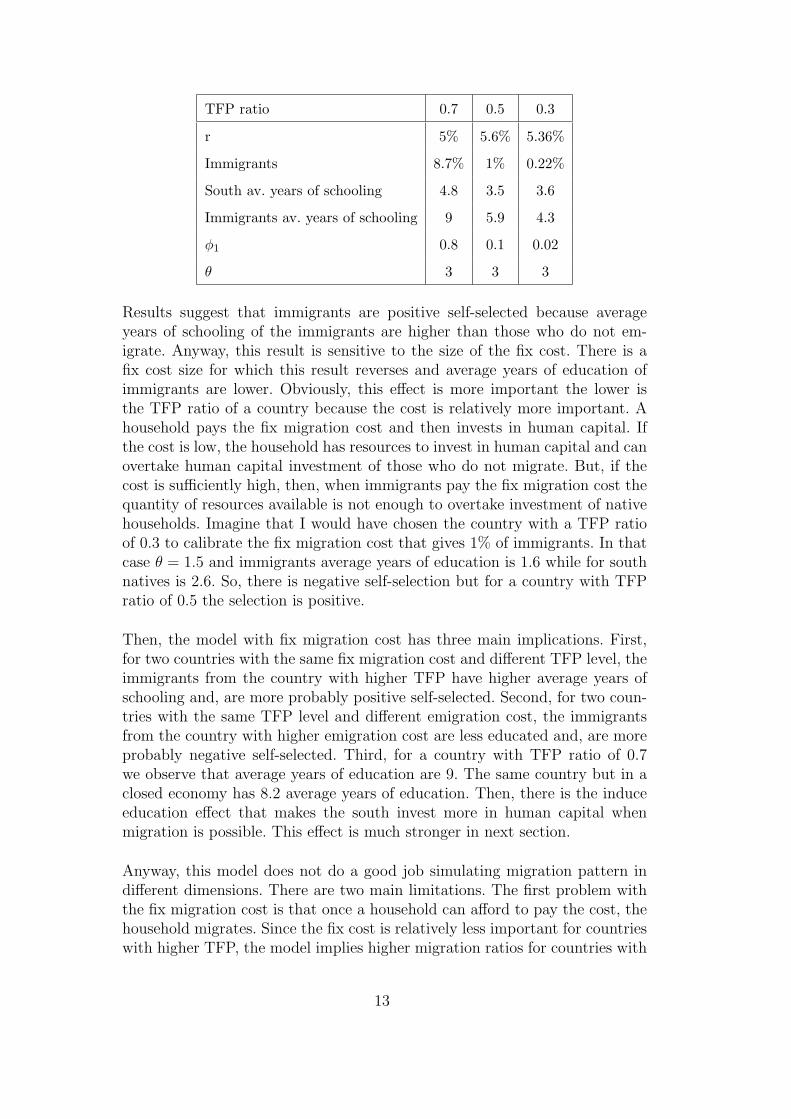
I set relative TFP ratios for Mexico and India to US as 0.6 and 0.3 respectively.Then, I fix θMf = 1. for Mexico and θIf = 3. for India. This tries to reflect thefact that the fix migration cost is higher from India than from Mexico. How doI choose θv for both countries? Since I know from previous studies the averageyears of schooling of the immigrants from these countries, I will calibrate theθMv and θIv that better match the data.

I find that with θMv = 0.22 and θIv = 0.32 average years of schooling forMexican immigrants is 7.2 and for Indian immigrants is 12.88. Moreover, av-erage years of schooling of Mexican natives is 5.1 and for Indian natives is4. Then, to match the data on average years of schooling the model suggeststhat the time migration cost is higher for Indian immigrants. There are sev-eral interpretations of this result. Could be that the distance to US affects toothe time migration cost in the sense that two countries close may have closercultures which makes easier the migration. Another explanation is that sincethe Mexican community is very important in US, this lower the time migra-

16

tion cost. This seems a good explanation and may be the way to estimatethe time migration cost with a better procedure in the future. Note that thisresult is very interesting because in the previous exercises I showed that forthe same calibrated costs, countries with higher TFP present stronger positiveself-selection than countries with low TFP. So, to increase the TFP helps toget positive self-selection. But India’s TFP is quite lower than Mexican’s TFP.Then, both costs are playing an important role in the pattern of self-selectionof immigrants.

Immigrants from Mexico represent 5% of Mexican population and Indian im-migrants are 0.001% of India. This result is mainly affected by the TFP ofeach country. Finally, I calculate the earnings ratio of the average immigrantto the average US native. For Mexican immigrants this ratio is 0.65 and forIndian immigrants is 0.83. Data for Mexican immigrant earnings says thatthey earn 40% less than a US native in average. In Hendricks these ratios are0.76 and 0.97 for Mexico and India respectively. The ratio has been adjustedfor identical age, education and sex.

A completely different case is UK. UK has TFP very similar to US. Averageyears of schooling of immigrants from UK is 14.6 while for UK the average is8.8. The adjusted ratio of earnings for an immigrant form UK with respectto a born-native in the US is 1.3. I fix TFP ratio equal to 0.9 and the fixmigration cost equal to 2, between the cost of Mexico and India. We expectthe time cost from UK to be very low. For a time cost equal to 0.025 I find thataverage years of immigrants from UK is 14.8. Moreover, the earnings ratio is1.2, reflecting that they earn more than US natives.

I sum up the results in the following table.

Mexico India UK

data model data model data model

TFP ratio - 0.6 - 0.3 - 0.9

θf - 1. - 3. - 2

θv - 0.22 - 0.33 - 0.025

Immigrants av. years of schooling 7.5 7.2 15.6 12.88 14.6 14.8

South av. years of schooling 6.3 5.1 5 4 8.8 6

Relative earnings 0.76 0.65 0.97 0.83 1.3 1.2

17

6 Implication in differences in output per capita across countries

7 Conclusion

I add the possibility of migration in a human capital growth model to answermainly two questions. First, investment in human capital is affected by thepossibility of future migration? And second, which is the pattern of selectionof immigrants? I find that optimal investment in human capital of immigrantsis clearly above the investment in human capital in a closed economy most ofthe cases. This supports the thesis of induce education effect of brain draintheory. The significance of the induce education effect depends on the relativesize of the migration costs, the TFP and the migration rate. Related with thisI find that the migration pattern of self-selection is not unique. For the samemigration costs Immigrants are positive self-selected for higher TFP countrieswhile they are negative self-selected for lower TFP countries. To increase thetime cost, all the rest constant, decreases the migration rate and implies higherpositive self-selection. For acceptable parameter values I find that the modelcan replicate real selection patterns of immigrants. I find that average yearsof Mexican immigrants is 7.2 and Mexican natives is 5.1 Data for Mexicanimmigrants is 7.5 and 6.3 for natives. For the Indian case I find a strongpositive self-selection as data indicates. I find that average years of schoolingis 12.88 for immigrants and 4 for natives. Data for Indian immigrants is 15.6and 5 for natives. I also get that immigrants from UK earns more than USnative. I find a earnings ratio of 1.2 when real ratio is 1.3. Average years ofschooling of immigrants from UK is 14.8 and in data it is 14.6.

The model has two main limitations. One has to be with dynamics of pop-ulation. Since in the steady state relative size of each country with respectto the world population must be constant, this implies a relationship betweenpopulation growth rates and migration rates. Moreover, for realistic migrationrates, the relative size of north is very small since south natural populationgrowth rate is higher. This affects comparative analysis because when I addimmigrants in the north, the mass of these immigrants is too high comparedto the north. The result is similar as in the north all the population are im-migrants. The second problem is that I need the fix migration cost if I donot want that everybody migrates. But if a household can pay the fix migra-tion cost, then migrates. So, in the steady state in the south there is not ahousehold that can pay the fix migration cost. Is like incentives to migrateare to high and this affects the results of the south native population that notmigrate.

These two problems show the line of future research. In fact, both limitationsof the model have to deal with the steady state equilibrium. The natural

18

progress has to be the computation of the transitions. It remains a carefullycalibration of the migration cost to match the model with different real cases.To solve this point it is crucial to find data on migration of human capital.Moreover, we can use the model to test different migration policies and itwould be interesting to add in the model complementarity and substitutivityof skills.

19

8 Appendix

8.1 Population Dynamics

I define N as total world population and the fraction of people living in countryi as φi = Ni

Nfor i = {0, 1}. Finally, I use the normalization φ0 + φ1 = 1. Using

these definitions and equations (2) and (1) I can write population dynamicsin the following way for both economies:

φ′

1 =(1 + n1)φ1 + (1 + n0)mφ0

(1 + n1)φ1 + (1 + n0)φ0

(3)

φ′

0 =(1 + n0)(1−m)φ0

(1 + n1)φ1 + (1 + n0)φ0

(4)

Equilibrium in the steady state implies that φ′i = φi for i = {0, 1}. It means

that the size of the population relative to the world population must be con-stant in each economy. Equivalently, it means that population growth ratesare equal in both economies in the steady state. Using this I obtain a necessarycondition for the steady state:

m = φn

(n0 − n1

1− n0

)(5)

8.2 Steady State Equilibrium

For notation porpoise set x = {a, h, z, i} and X = {[0,∞]×[0,∞]×Z×{0, 1}}.Let B be the σ − algebra generated in X by the Borel subsets. A probabilitymeasure µ over B describes the economy by stating how many households thereare of each type. Let P (x,B) denote the transition function. Function P de-scribes the conditional probability for a type x household to have a type in theset B ⊂ B tomorrow and describes how the economy moves over time by gen-erating a probability measure for tomorrow, µ

′, given a probability measure,

µ today. So, µ′(B) =

∫X P (x,B)dµ is tomorrow distribution of households µ

′

as a function of today’s distribution µ and the Markov chain.Let X0 be X |i=0 and X1 be X |i=1 and equivalently for xi. Set gj(x) asthe policy function for j = c, a, h, e, s, i. The steady state equilibrium for thiseconomy is a set of functions for the household’s problem {v(x), gc(x), ga(x),gh(x), ge(x), gs(x), gi(x)}, prices wi and r and a measure of households, µ,such that:

(1) Markets are competitive and there are no arbitrage opportunities. Note

20

that since capital is freely perfect mobile, capital rental price must equal-ize across countries. Then factors rental prices are:

r=αA0

(K0

H0

)α−1

= αA1

(K1

H1

)α−1

wi = (1− α)Ai

(Ki

Hi

)α(2) Given µ, aggregate factors and prices, the functions {v(x), gc(x), ga(x),

gh(x), ge(x), gs(x), gi(x)} solve the household’s problem.(3) Population growth rates are equal in both economies, equation (5) holds.(4) Markets clear:

Hi =∫Xi

h dµ(xi) +∫Xi

(1− gs(xi))ψ dµ(xi) for i = {0, 1}

K0 +K1 =∫Xa dµ(x)

I =∫X

[ga(x)− (1− δ)a] dµ(x)

(5) The world resource constraint is satisfied:

Y0 + Y1 =∫X

[gc(x) + ge(x)] dµ(x) + I +∫X0

gi(x0)θ dµ(x0)

(6) The measure of households is stationary µ(B) =∫X P (x,B) dµ

21

References

Barro, R. J. and J. W. Lee (1996, May). International measures of schoolingyears and schooling quality. American Economic Review 86 (2), 218–23.

Borjas, G. J. (1994, December). The economics of immigration. Journal ofEconomic Literature 32 (4), 1667–1717.

Cooley, T. F. and E. C. Prescott. Economic growth and business cycles.Erosa, A., T. Koreshkova, and D. Restuccia (2007, March). How important

is human capital? a quantitative theory assessment of world income in-equality. Working Papers tecipa-280, University of Toronto, Departmentof Economics.

Gollin, D. (2002, April). Getting income shares right. Journal of PoliticalEconomy 110 (2), 458–474.

Haveman, R. and B. Wolfe (1995, December). The determinants of chil-dren’s attainments: A review of methods and findings. Journal of Eco-nomic Literature 33 (4), 1829–1878.

Keane, M. P. and K. I. Wolpin (2001, November). The effect of parentaltransfers and borrowing constraints on educational attainment. Inter-national Economic Review 42 (4), 1051–1103.

Klein, P. and G. Ventura (2007). Productivity differences and the dynamiceffects of labor movements. Working papers.

Seshadri, A. and R. Manuelli (2007). Human capital and the wealth ofnations. Technical report.

Tauchen, G. (1986). Finite state Markov-chain approximations to univariateand vector autoregressions. Economics Letters 20, 177–181.

22