Quantitative analysis of water poverty

in England and Wales

Water UK

March 2021

FINAL REPORT

2

Important notice

This document was prepared by CEPA LLP (trading as CEPA) for the exclusive use of the recipient(s) named

herein.

The information contained in this document has been compiled by CEPA and may include material from other

sources, which is believed to be reliable but has not been verified or audited. Public information, industry and

statistical data are from sources we deem to be reliable; however, no reliance may be placed for any purposes

whatsoever on the contents of this document or on its completeness. No representation or warranty, express or

implied, is given and no responsibility or liability is or will be accepted by or on behalf of CEPA or by any of its

directors, members, employees, agents or any other person as to the accuracy, completeness or correctness of the

information contained in this document and any such liability is expressly disclaimed.

The findings enclosed in this document may contain predictions based on current data and historical trends. Any

such predictions are subject to inherent risks and uncertainties.

The opinions expressed in this document are valid only for the purpose stated herein and as of the date stated. No

obligation is assumed to revise this document to reflect changes, events or conditions, which occur subsequent to

the date hereof.

CEPA does not accept or assume any responsibility in respect of the document to any readers of it (third parties),

other than the recipient(s) named therein. To the fullest extent permitted by law, CEPA will accept no liability in

respect of the document to any third parties. Should any third parties choose to rely on the document, then they do

so at their own risk.

The content contained within this document is the copyright of the recipient(s) named herein, or CEPA has licensed

its copyright to recipient(s) named herein. The recipient(s) or any third parties may not reproduce or pass on this

document, directly or indirectly, to any other person in whole or in part, for any other purpose than stated herein,

without our prior approval.

3

Contents

FOREWORD .................................................................................................................................... 4

EXECUTIVE SUMMARY ..................................................................................................................... 6

1. INTRODUCTION ...................................................................................................................... 13

1.1. Context .................................................................................................................................... 13

1.2. Modelling objectives .............................................................................................................. 13

1.3. Scope of project ..................................................................................................................... 14

1.4. Structure of report ................................................................................................................. 14

2. METHODOLOGY ..................................................................................................................... 15

2.1. Modelling framework ............................................................................................................. 15

2.2. Input assumptions .................................................................................................................. 17

2.3. Distributional assumptions .................................................................................................... 20

2.4. Monte-Carlo simulation ......................................................................................................... 24

2.5. Interpretation of outputs........................................................................................................ 25

3. DATA .................................................................................................................................... 27

3.1. Bill distribution ........................................................................................................................ 27

3.2. Income distribution ................................................................................................................ 29

4. WATER POVERTY IN 2019/20 .................................................................................................. 30

4.1. Main results ............................................................................................................................. 30

4.2. Geographical variation .......................................................................................................... 34

4.3. Threshold sensitivity analysis ............................................................................................... 37

5. INDICATIVE IMPACT OF INTERVENTIONS ..................................................................................... 38

5.1. Context .................................................................................................................................... 38

5.2. Approach to estimation ......................................................................................................... 40

5.3. Initial estimates of current company interventions ........................................................... 41

6. CONCLUSIONS AND NEXT STEPS ............................................................................................... 45

DETAILED METHODOLOGY ...................................................................................... 46

FULL RESULTS ....................................................................................................... 54

SENSITIVITY TESTING .............................................................................................. 65

4

FOREWORD

Following on from our 2020 pathfinder study of water poverty measurement1, CEPA is pleased to present in this

report, on behalf of Water UK, the results of our further work to develop and implement an approach for estimating

the scale of water poverty in England and Wales as of 2019/20.

Though the scope of this work is technical in nature we are conscious that water poverty, and potential

interventions to address it, is a live area of current policy debate, not least in the context of the CCW Affordability

Review2. We therefore begin our report with some observations to aid readers in interpreting our work and to help

inform the wider debate in the area, drawing on our experience.

Ultimately, the industry and its stakeholders share a desire to make bills for an essential service affordable for all

households. To our knowledge there are currently no industry-wide estimates of water poverty that are able to draw

on consistent company-level data on bills. Although we recognise that there may be a range of viable approaches

to defining and measuring water poverty at different levels of aggregation – and so the results in this report cannot

give a definitive position – this study represents an important ‘first of a kind’ attempt to provide consistent,

replicable industry-wide coverage.

We estimate an overall industry-wide level of water poverty that is broadly consistent with previous studies, but also

show that there is considerable variation in its incidence across the country – including large differences within and

between supply areas. Any interventions to address water poverty could therefore have quite different implications

for customers in different regions, in addition to existing variations in the degree of support provided.

Whilst this report therefore adds to the growing evidence base concerning water poverty and affordability, it is

important for policymakers and other stakeholders to bear the following key points in mind when reviewing and

using the analysis and results of our study:

• We recognise that water poverty is a multi-faceted issue that can be defined and measured in different

ways. Our previous work for UKWIR surveys these issues.3 For this study we have been asked by Water UK

to estimate water poverty using a ratio of customer bills to income based on a defined set of water poverty

thresholds (bill to income ratios of 3% and 5%); we have also tested the sensitivity of our analysis to a range

of different thresholds.

• The purpose of this study is not to provide guidance on policy options to address water poverty, and we

were not asked to model or analyse potential water poverty interventions or policies. While we hope that

our analysis can play a role in helping to inform subsequent policy debates, we would caution against over-

interpreting the results presented in this report.

• Though we present analysis based on different water poverty thresholds, using a bills to income metric, we

make no judgement as to the appropriateness of any particular threshold. The analysis highlights

quantitatively different objectives that could be considered – for instance, focussing on the number of

households in water poverty as distinct from the degree of water poverty – but does not make or imply any

judgement as to how competing or overlapping objectives might best be balanced.

• We have focused on producing a snapshot of water poverty based on a simulation approach that neither

relies on household level input data nor produces output data relating to specific actual households. This

supports replicability over time and allows us to present consistent industry-wide estimates – but there are

natural sources of uncertainty in this approach, particularly when making comparisons between regions.

———————————————————————————————————————————————————

1 CEPA, August 2020. Measuring water poverty using a bills to income metric. Available here.

2 CCW, October 2020. CCW Affordability Review. Available here.

3 UKWIR, March 2020. Defining water poverty and evaluating existing information and approaches to reduce water poverty.

Available here.

5

• Our approach allows us to provide preliminary analysis of the impact of existing policy interventions, such

as social tariffs, against the measure of water poverty used in this report. These results are, however,

particularly sensitive to input assumptions, and there is no clear benchmark against which to compare

these interventions. These results are therefore not intended as an evaluation of existing policies or

interventions, or any implied comment on whether these policies or interventions should be maintained or

amended. They should instead be interpreted as an initial, indicative view to stimulate discussion and to

help set context for future work.

• We present several statistics on a normalised basis – for example, figures per household in water poverty

or per household not in water poverty. These are intended to help the reader gauge relative levels of water

poverty across regions which may have significantly different sizes of customer base. However, particular

caution is needed in seeking to interpret these figures from a policy perspective.

• In particular, our calculations of the ‘water poverty gap’ indicate a strictly theoretical minimum ‘cost’ of

eradicating water poverty at a given bill to income ratio threshold, if it were possible to perfectly target

interventions. Whilst this water poverty gap offers an informative theoretical reference point, in practice it is

not a directly or perfectly targetable metric for designing or assessing such interventions, so actual costs

for eradicating water poverty would be higher. It is also important to note that these calculations are based

on the status quo position – that is, the water poverty gap is the gap that still remains after current

interventions like social tariffs, and implicitly assumes that these interventions are maintained.

• The ongoing debate in the sector will need to address issues of targeting, calibrating and funding policies

and interventions to address water poverty, and it is likely that a number of options could be considered.

Though our analysis provides important context to help guide such work, it has not been developed to

directly test questions around intervention design and effectiveness.

We look forward to ongoing engagement and debate on these issues in the coming months.

6

EXECUTIVE SUMMARY

Context

Approximately three million customers in the UK say that they struggle to pay their water bills.4 In April 2019, as part

of increased ambition within the sector to address affordability, the English water industry adopted a Public Interest

Commitment (PIC) to:

“make bills affordable as a minimum for all households with water and sewerage bills more than

5% of their disposable income by 2030 and develop a strategy to end water poverty.” 5

Achieving this PIC requires the estimation of water poverty at national and regionally disaggregated levels to

understand current levels of water poverty and to track industry progress. The overall purpose of this project is to

provide such estimates and a methodological basis for updating them over time.

Our findings will also provide evidence for the CCW Affordability Review6 announced in October 2020, an

independent review of current financial support measures to identify opportunities to improve the help available to

financially vulnerable households.

Scope and objectives

CEPA has been commissioned by Water UK to develop and implement an approach for estimating the scale of

water poverty in England and Wales as of 2019/20, using a consistent approach across individual companies,

sectors and regions. This report includes results on:

• baseline (2019/20) water poverty levels in England and Wales; and

• the monetary ‘water poverty gap’, i.e. the theoretical minimum amount of support required to eliminate

water poverty at a given threshold.

For this study we have been asked by Water UK to define water poverty based on the ratio of a household’s water

and sewerage bills to its income (with the definition of income outlined further below). In line with common

approaches to assessing water poverty we focus on two thresholds at which a household might be defined as water

poor: a 3% and a 5% ratio of bills to income.

The water poverty gap reflects a theoretical minimum ‘cost’ of eradicating water poverty at a given bill to income

ratio threshold. It is a useful metric for understanding, on a consistent basis, the scale and materiality of the water

poverty challenge in England and Wales at different bill to income thresholds. However, we would not consider the

water poverty gap to be a directly and perfectly targetable metric for designing water poverty interventions.

For example, if the water poverty gap is found to be £x million for a given threshold, we would not consider it to be

possible to perfectly target an intervention of £x million (e.g., a transfer between non-water poor and water poor) to

close this monetary gap but strictly no more than that. In practice, to substantially close the water poverty gap

would be likely to require both changes in the approach to interventions to target this specific definition of water

poverty and higher levels of support than the calculated water poverty gap. There would be substantial challenges

in perfectly targeting interventions to achieve no more than a target threshold.

As a secondary objective, the modelling approach we have developed allows us to carry out exploratory analysis of

the impact of interventions currently in place within the sector, such as social tariffs, against the measure of water

poverty defined in this project. This is a more challenging area to address using an industry-wide approach and

data sources, and our results are necessarily more preliminary in nature.

———————————————————————————————————————————————————

4 Ofwat, December 2019. PR19 final determinations. Available here.

5 Water UK, April 2019. Water industry reaffirms pledge to work in the public interest. Available here.

6 CCW, October 2020. CCW Affordability Review. Available here.

7

We have not sought to estimate a detailed, disaggregated distribution of the degree to which individual households

are water poor. However, by calculating sensitivity tests of water poverty estimates at different thresholds we are

able to form some high level impressions of the distribution of water poverty. This work is not intended to develop

or test water poverty policy implications and caution should be exercised in interpreting these results – though

clearly the targeting, calibration and funding of any support designed to address water poverty are critical issues

that follow-up analysis would need to inform.

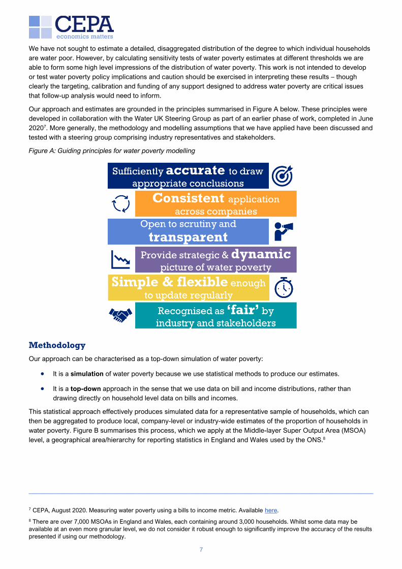
Our approach and estimates are grounded in the principles summarised in Figure A below. These principles were

developed in collaboration with the Water UK Steering Group as part of an earlier phase of work, completed in June

20207. More generally, the methodology and modelling assumptions that we have applied have been discussed and

tested with a steering group comprising industry representatives and stakeholders.

Figure A: Guiding principles for water poverty modelling

Methodology

Our approach can be characterised as a top-down simulation of water poverty:

• It is a simulation of water poverty because we use statistical methods to produce our estimates.

• It is a top-down approach in the sense that we use data on bill and income distributions, rather than

drawing directly on household level data on bills and incomes.

This statistical approach effectively produces simulated data for a representative sample of households, which can

then be aggregated to produce local, company-level or industry-wide estimates of the proportion of households in

water poverty. Figure B summarises this process, which we apply at the Middle-layer Super Output Area (MSOA)

level, a geographical area/hierarchy for reporting statistics in England and Wales used by the ONS.8

———————————————————————————————————————————————————

7 CEPA, August 2020. Measuring water poverty using a bills to income metric. Available here.

8 There are over 7,000 MSOAs in England and Wales, each containing around 3,000 households. Whilst some data may be

available at an even more granular level, we do not consider it robust enough to significantly improve the accuracy of the results

presented if using our methodology.

8

Figure B: Summary of top-down approach

This approach allows us to:

• produce water poverty estimates at a granular level without imposing disproportionate demands on the

amount of data required;

• segment our analysis by different household or tariff characteristics; and

• estimate counterfactual scenarios for some segments, which can in principle be used to assess the impact

of interventions and policies.

This approach should be seen as complementary to existing approaches and estimates of water poverty levels in

regions or all of England and Wales. In some cases it is possible to use highly disaggregated data to produce more

direct measurements. A distinguishing feature of our approach is that it produces industry-wide estimates on a

consistent basis across companies in a way that is highly repeatable over time.

In addition to bill distribution data provided by companies, our estimates are based on ONS data on income

distributions. Our estimates are based on equivalised disposable (post-tax) income after housing costs in order to

reflect the standard of living a household’s income is capable of delivering. We accommodate disability payments

for a subset of households in our analysis.

We adjust the national income distribution data to reflect MSOA average income, and apply a truncated income

distribution for analysis of customer segments receiving discounted bills.9 A key model input is the assumed

correlation between household bills and income, which we base on household level survey data.

Estimates of water poverty

The results of our simulation analysis fall into two categories:

1. For each MSOA we estimate incidence of water poverty, i.e., the proportion of households that would be

defined as water poor for a chosen threshold. Based on the number of households in a MSOA we can then

translate this into the implied number of water poor households.

2. Based on each simulated household’s distance (in monetary terms) from the chosen threshold, we also

estimate the overall water poverty ‘gap’ for each MSOA. As discussed above, this represents the theoretical

———————————————————————————————————————————————————

9 Households receiving discounted bills are assumed to be at the lower end of the national distribution, with net disposable

incomes less than roughly £16,000 (around £19,000 in London). Other households are drawn from the national income

distribution, after accounting for the fact many at the lower end will be receiving discounted bills.

9

minimum amount of support required to bring each household to the water poverty threshold (and no further).

This figure can also be expressed as an average amount (£) per water poor household or an amount (£) per

non-water poor household.

Table A below presents our main results at an industry and national level. The incidence of water poverty is

sensitive to the choice of threshold, with nearly three times as many households defined as water poor at the 3%

threshold as at the 5% threshold. In addition to these results at the thresholds most commonly used in the water

sector, we have also carried out sensitivity tests at various different thresholds to improve understanding of how the

level of water poverty varies with the choice of threshold (see Section 4.3 of the main report).

Table A: Estimated water poverty by region, 2019/20

Region 5% threshold 3% threshold

Incidence Households Incidence Households

Industry 6.5% 1,468,000 17.9% 4,066,000

England 6.3% 1,354,000 17.4% 3,712,000

Wales 8.7% 114,000 27.2% 354,000

Source: CEPA analysis

There is considerable variation by company and by local area, as shown in Figures C and D below.10

Figure C: Estimated water poverty incidence by company, 2019/20

Source: CEPA analysis

———————————————————————————————————————————————————

10 A key of the company acroynms used in figures throughout the report can be found as part of Appendix A.

10

Figure D: Estimated water poverty by MSOA at 5% threshold, 2019/20

Source: CEPA analysis

Table B presents our estimates of the industry and regional water poverty gap.

Table B: Estimated water poverty gap by region, 2019/20

5% threshold 3% threshold

Total water

poverty gap

Gap per water

poor hh

Gap per non-

water poor hh

Total water

poverty gap

Gap per water

poor hh

Gap per non-

water poor hh

Industry £236 m £161 £11 £720 m £177 £39

England £220 m £162 £11 £663 m £179 £38

Wales £16 m £138 £13 £57 m £161 £60

Company range 1 £128 to £253 £4 to £32 £138 to £276 £14 to £102

Source: CEPA analysis. Note 1: Lowest and highest company values in the sector for each measure

Two features are apparent when expressing the gap on a per household basis. The gap per water poor household

is similar whether using the 3% threshold or the 5% threshold: applying the lower 3% threshold increases the

distance from the threshold for those households that are water poor at the 5% threshold – but this effect is offset

by the inclusion of additional households that by definition are relatively close to the threshold. The gap per non-

water poor household is particularly sensitive to the choice of threshold – since it is affected both by the change in

size of the gap and the change in the number of households included in the denominator. This helps to illustrate the

exponential nature of the challenge in eliminating water poverty at progressively lower thresholds.

11

As discussed above, it is also important to note that our findings on the water poverty gap cannot provide any

conclusions as to the feasibility of targeting and calibrating such support to eradicate water poverty at a defined

threshold level. The water poverty gap reflects a theoretical minimum ‘cost’ of of eradicating water poverty at a

given bill to income ratio threshold. Precise targeting of support would require extensive information to calibrate

new and existing interventions to our new methodology that may simply not be available or usable operationally.

This means in practice that significantly higher levels of support would be needed than the calculated water poverty

gap to bring all customers below a given threshold.

Interventions

Analysis of the impact of existing water poverty interventions is more challenging to produce and interpret. In

applying a common, industry-wide approach to simulating water poverty we have necessarily applied a simplifying

assumption regarding the targeting of current direct financial support to simulated households.

Our results on intervention impacts – which are defined as the difference between water poverty incidence before

and after intervention – are particularly sensitive to these modelling assumptions. Estimates produced using a

common industry-wide approach may not correspond precisely to companies' own estimates, which may be based

on more bespoke modelling approaches, or more granular data sets.

It should also be noted that our approach to measuring water poverty is new and being used on an industry-wide

basis in this report for the first time. Current interventions were therefore not designed or intended to maximse the

reduction in water poverty when measured using this specific approach. As such, this analysis should not be

interpreted as an assessment of the appropriateness of current interventions.

Nevertheless, our simulation results give an indication of the impact of current interventions in relation to our

methodology. Table C below summarises our results at the industry and region level.

Table C: Estimated impact of interventions at 3% and 5% threshold by region

Region Pre-intervention

water poverty rate

Reduction in water

poverty rate from

interventions

Households moved

below poverty

threshold

Reduction in total

water poverty gap

3% threshold

Industry 18.9% -1.0% -226,000 -£131 m

England 18.2% -0.8% -179,000 -£103 m

Wales 30.8% -3.6% -47,000 -£28 m

5% threshold

Industry 7.6% -1.2% -263,000 -£89 m

England 7.3% -0.9% -203,000 -£72 m

Wales 13.4% -4.7% -61,000 -£17 m

Source: CEPA analysis

It is important to note that the number of households moved below the poverty threshold in Table C does not

include households whose bill to income ratios are reduced via company interventions, but remain above the 3% or

5% threshold. Some households may be provided with substantial financial support, but remain above the threshold

due to the extent of their pre-intervention water poverty. The impact on these households (up to and no further than

the 3% or 5% threshold) is, however, captured in the reduction in the total water poverty gap.

For example, company support may reduce a household’s bill to income ratio from 8% to 6%, or from a 4.5% ratio

to 3.5%. Neither of these households would be included in the number of households moved below the poverty

threshold in our analysis, as neither has gone below the relevant threshold. However, the financial support provided

to them would be included in the reduction in the total water poverty gap. A consequence of this is that the number

of households estimated to move below the water poverty threshold in our analysis – as strictly defined in Table C –

12

is substantially below the number of households that are known to receive support from one of the two main

schemes in England and Wales, i.e., WaterSure and company social tariffs.11

Finally, it is important to note there may be a degree of ‘overlap’ between the estimated reduction in households in

water poverty at the 3% and 5% thresholds. For example, a household whose bill to income ratio is reduced from

6% to 2.5% would be included in both the 3% and 5% estimate of households moved below the relevant water

poverty threshold. It is also not meaningful to consider the reduction in water poverty (£) per household taken out of

water poverty in Table C (i.e. dividing “Reduction in total water poverty gap” by “Households moved below poverty

threshold in water poverty”), since different populations are considered for the two measures.

Conclusions and next steps

The results of this study demonstrate the feasibility of using a top-down simulation approach to estimating the

incidence of water poverty at the industry, regional and company level in England and Wales. We estimate an

overall industry-wide level of water poverty that is broadly consistent with previous studies. These estimates can be

replicated in order to consistently monitor water poverty over time. The results also show that there is considerable

variation in its incidence across the country – including large differences within and between supply areas. Any

interventions to address water poverty could therefore have quite different implications for customers, in addition to

existing variations in the degree of support provided.

Turning to policy implications, it is for the water sector to consider whether it wishes to adopt this approach as the

standard basis for assessing water poverty across England and Wales. If so, three particular issues would be

relevant:

• Targeting of support – which households should be defined as being in water poverty and requiring

support? How closely could (in theory) and should (in practice) support be targeted (or re-targeted in the

case of existing support schemes) to maximise the impact against the measure of water poverty used in

this study? This is particularly sensitive to the choice of water poverty threshold, with our analysis indicating

that around 11.5% of households across England and Wales fall between the 3% and 5% bill to income ratio

thresholds commonly used to define water poverty.

• Calibration of support – how much support do different households require, and how closely could (in

theory) and should (in practice) the level of support for a household be calibrated to maximise the impact

against the measure of water poverty used in this study? Our analysis indicates that at least a further

£236m would be required to eliminate water poverty at the 5% threshold, or £720m at the 3% threshold.

The actual value of support required would exceed this, however, assuming that it is not practical to

perfectly target and calibrate support. There is also an important challenge in valuing support that (a) may

move a household closer to but not beyond a given threshold, or (b) may be provided to a household that is

marginally outside the definition of water poverty but may still be in financially vulnerable circumstances.

• Funding of support. Though we have expressed the water poverty gap on a per non-water poor household

basis for illustrative purposes, in practice cross-subsidisation of water bills is only one potential policy

choice, and cross-subsidation could be carried out on an individual company basis, a regional basis or an

industry-wide basis. Our analysis – particularly that based on the lower 3% threshold for defining water

poverty – indicates that the implied support per non-water poor household may be substantial. Any further

interventions funded by bills may need to consider second-order impacts on water poverty as a result of

elevated standard tariffs.

Further analysis could help further inform these issues. The scope of the modelling could be further expanded and

refined to include more detailed data on the distribution of household-level water poverty, in addition to its

incidence at defined thresholds of the ratio of bills to income. More detailed analysis of the impact of interventions

would benefit from developing a more bespoke approach to assumptions on customer segmentation, income

distribution and the correlation between bills and income. Each of these refinements could be applied within the

framework of the simulation approach we have developed.

———————————————————————————————————————————————————

11 Information collated by CCW indicates that there were around 900,000 customers supported by either WaterSure or a form of

social tariff in England and Wales in 2019/20.

13

1. INTRODUCTION

Approximately three million customers in the UK say that they struggle to pay their water bills.12 In April 2019, as

part of increased ambition within the sector to address affordability, the English water industry adopted a Public

Interest Commitment (PIC) to:

“make bills affordable as a minimum for all households with water and sewerage bills more than

5% of their disposable income by 2030 and develop a strategy to end water poverty.” 13

Achieving this PIC requires the estimation of water poverty at national and regionally disaggregated levels to

understand current levels of water poverty and to track industry progress. This project was commissioned by Water

UK to provide estimates of current (2019/20) levels of water poverty in England and Wales and an estimation of the

monetary size of the ‘water poverty / affordability gap’.

1.1. CONTEXT

CEPA’s work for Water UK has been commissioned to build on the findings of the project carried out by CEPA and

Sustainability First for UKWIR14, which sought to develop a clear understanding of what is meant by water poverty;

assess metrics that could be used to measure it; identify the fundamental drivers of water poverty; and summarise

the range of approaches which water companies may use to alleviate it. A key finding of the work was that “the

most suitable metric is likely to be a percentage of disposable income metric”. Building on this finding, CEPA was

asked to produce a report for Water UK on the methodological choices that needed to be made to be able to

calculate a ‘bills to income’ metric of water poverty in a common manner across England and Wales15.

In this project, we build on this previous analysis to apply our methodology across England and Wales, to estimate

baseline (2019/20) levels of water poverty and the monetary ‘water poverty gap’ on a consistent basis across the

industry. Our findings will feed into the CCW Affordability Review16 announced in October 2020, comprising an

independent review of current financial support measures to identify opportunities to improve the help available to

financially vulnerable households.

1.2. MODELLING OBJECTIVES

Proof of concept model (‘Phase One’)

Our initial work for Water UK in early 2020 (‘Phase One’) undertook proof-of-concept modelling for calculating

water poverty in England and Wales. This included:

• Assessing possible levels of geographic aggregation, such as Middle Layer Super Output Areas

(MSOAs), and the associated impact on analytical approaches and data availability.

• Examining the definition of income, in relation to data availability, the treatment of housing and childcare

costs, and the effects of equivalisation on household incomes.

• Developing a ‘proof-of-concept’ model to demonstrate the feasibility of a statistical approach to

estimating levels of water poverty for a selection of water companies.

———————————————————————————————————————————————————

12 Ofwat, December 2019. PR19 final determinations. Available here.

13 Water UK, April 2019. Water industry reaffirms pledge to work in the public interest. Available here.

14 UKWIR, March 2020. Defining water poverty and evaluating existing information and approaches to reduce water poverty.

Available here.

15 Water UK, August 2020. Measuring water poverty using a bills to income metric. Available here.

16 CCW, October 2020. CCW Affordability Review. Available here.

14

• Estimating the impact of different income assumptions by applying a proof-of-concept model under

varying assumptions.

Extending analysis (‘Phase Two’)

In this ‘Phase Two’ project, we have built on the Phase One analysis to:

• Estimate baseline (2019/20) water poverty levels in England and Wales using a consistent approach

across individual companies, sectors and regions.

• Estimate the monetary ‘water poverty gap’: i.e., what is the theoretical minimum amount of support

required to eliminate water poverty at a given threshold.

• Extend the approach in Phase One to water-only companies.

• Compare results to more detailed calculations undertaken by companies.

• Address outstanding methodological issues from Phase One.

1.3. SCOPE OF PROJECT

The scope of this work focuses on the incidence of, and direct financial support aimed at alleviating, water poverty

for the 17 incumbent companies that provide household retail and wholesale water and sewerage services in

England and Wales. Building on the findings of the UKWIR study, we have been asked by Water UK to use the bill to

income metric to measure water poverty for this study, but recognise that there are other potential measures which

may capture different aspects of water poverty.

Given the objective to understand and monitor levels of water poverty across England and Wales, our approach can

be considered as ‘top-down’, and complementary to (rather than a replacement for) ‘bottom-up’ assessments which

use data from specific individual households and are currently employed by a number of water and sewerage

companies in England and Wales to both monitor and target support for households in water poverty.

We also highlight that this project does not estimate levels of water poverty in Scotland or Northern Ireland or

forecast future changes in water poverty. The Covid-19 pandemic and other drivers of bill levels in England and

Wales are also important issues in affordability, but out of scope for this analysis, not least because the analysis has

been carried out on data for the year 2019-20, during which Covid-19 had a more limited impact on the water

industry.

1.4. STRUCTURE OF REPORT

The remainder of this report is structured as follows:

• Section 2 sets out our methodology.

• Section 3 discusses our approach to data collection, processing and aggregation.

• Section 4 describes the main results of our analysis.

• Section 5 presents some initial analysis assessing the impact of interventions by water sector stakeholders

on estimated levels of water poverty.

• Section 6 provides concluding remarks and sets out potential next steps.

Readers interested in the results may wish to focus on Sections 4-6, as Sections 2-3 are intended to provide full

technical details of our methodology. Appendices include a detailed description of various methodological

assumptions and processes (Appendix A), the full results from our analysis (Appendix B) and results from sensitivity

tests (Appendix C).

15

2. METHODOLOGY

In this section we describe our methodological approach to estimating water poverty in England and Wales. This

approach has been developed by drawing on our expert knowledge and experience, a consideration of existing

methodologies, and most importantly discussions with key stakeholders.

Building on the progress made developing the proof of concept models, Water UK, water company representatives

and other key industry stakeholders were involved to develop the methodology. Methodological workshops and

working notes were used to refine the approach described below and to help stakeholders agree a consistent

industry-level method for how a ‘bills to income’ metric would be calculated and modelled.

We summarise at a high level our estimation process in the Figure 2.1 below:

Figure 2.1: High-level methodological process

The following subsections explore each of these steps in turn. We start by introducing our general modelling

approach for this analysis at a high level, and then we set out the justification for key methodological assumptions.

This provides context for further discussion of the ‘engine’ of our model – where we simulate households to

generate a statistical approximation for water poverty and associated outputs. Finally, we provide further guidance

on how to interpret the results of our analysis.

2.1. MODELLING FRAMEWORK

2.1.1. Model principles

During the proof of concept phase, water companies and water sector stakeholders came together to agree a high-

level methodology for how a ‘bills to income’ metric would be calculated and modelled, and to define the potential

scope for modelling and data requirements for possible subsequent work. As part of this process, six Guiding

Principles to guide the analysis were developed and had broad support from the Project Steering Group.

Figure 2.2 summarises the Guiding Principles, which state the methodology and model:

• Should provide a strategic and dynamic picture of current and future levels of water poverty, such that the

progress in reducing water poverty could be demonstrated and tracked.

• Must be consistent in application across companies.

• Are transparent, in an environment where companies need to demonstrate legitimacy and support for

affordability. In practice, this is likely to mean that the methodology and resulting measure of water poverty

needs to be able to be scrutinised.

• Are sufficiently simple and flexible to model and update in the timescales available each year that the

calculations need to be performed.

• Are sufficiently accurate to draw appropriate conclusions of progress towards the goal of reducing water

poverty.Should be seen as ‘fair’ within the industry and to external stakeholders, recognising that there are

likely to be different perspectives on the definition of ‘fairness’.17

———————————————————————————————————————————————————

17 We did not apply a formal definition of fairness for this work, but considered how a measure would be perceived within the

industry and by stakeholders. There is a distinction between a fair measure and a fair response to addressing water poverty, and

more formal approaches may be needed to ensure that responses to water poverty are fair, for example being fair in the burden

carried by different groups.

Modelling framework

Input assumptions

Distributional assumptions

Simulation Outputs

16

Figure 2.2: Guiding Principles for water poverty modelling

The methodology used in the following analysis was developed with these Guiding Principles in mind. For example,

we focused on using publicly available data, where this did not compromise accuracy, and generating repeatable

outputs to ensure transparency. A ‘bottom-up’ approach – where bill and income data from actual customers is

collected across the target population – could also be a data-intensive and costly process to update regularly.18

2.1.2. Top-down approach

Therefore, in line with the Guiding Principles, we developed a form of ‘top-down’ analysis for our analysis. Rather

than directly determining whether each actual household should be considered water poor, this approach uses

statistical assumptions about the distribution of bills and incomes to simulate a representative sample of

households. A bill to income ratio can then be calculated for each hypothetical household, which is then aggregated

to, for example, a company-level estimate of the proportion of households in water poverty.

Figure 2.3 summarises this process. The remaining subsections explore the components in further detail.

———————————————————————————————————————————————————

18 The Phase One report provides further detail of the advantages and disadvantages of different modelling approaches. CEPA,

August 2020. Measuring water poverty using a bills to income metric.

17

Figure 2.3: Summary of top-down approach

The top-down approach has a number of useful characteristics in addition to being consistent with our Guiding

Principles. In particular, the framework allows for different distributional assumptions to be made for different types

of customer. This can be considered over three key dimensions:

• Locational: the approach enables estimates to be produced at a granular level, without requiring very high

data requirements, by adjusting the distributions used according to location. As discussed in Section 2.2,

our analysis is conducted at a Middle-layer Super Output Area (MSOA) level. There are over 7,000 of these

geographical zones in England and Wales, each containing around 3,000 households.

• Household / tariff characteristics: certain groups of customers might have lower household income (and

therefore be more likely to be at risk of water poverty, all other things equal). However, these are likely the

customers that water companies will try to target with affordability support. This will mean such groups

could have markedly different distributions of both their bills and income compared to a company’s ‘typical’

customer. As discussed in Section 2.3, our analysis segments households into four groups – metered or

unmetered and ‘standard’ or ‘discounted’. However, in principle this framework allows scope for even more

bespoke assumptions to be made by further segmentation.

• Impact analysis: it is possible to use different bill distributions for the same simulated household in order to

estimate the impact of water company affordability interventions. In other words, it is possible to simulate

water poverty pre-intervention (i.e., all customers face a form of standard charge, whether metered or

unmetered); and post-intervention (i.e., once company interventions (e.g. social tariffs) are accounted for).

This is explored further in Section 5.

While we consider the outputs presented to be suitably robust for the purposes of this project, a benefit of using

this flexible and repeatable top-down framework is that assumptions can be further refined as inputs become

available to improve estimates over time. This is particularly valuable in the context of a consistent modelling

approach to estimating water poverty when companies apply a varied range of approaches to affordability

challenges, but these can be highly specific in nature.

2.2. INPUT ASSUMPTIONS

In Sections 2.2 and 2.3 we provide a high level summary of the key assumptions used in our modelling of water

poverty. Further detail can be found in Appendix A.

18

Summary of input assumptions

• Regarding income inputs, we choose to use net (of taxes) equivalised income after housing costs and

adjusted for disability allowances.

• We choose to aggregate data to the Middle Layer Super Output Area (MSOA) level, where there is greater

data availability.

• We measure the incidence of water poverty as the proportion of households with combined water and

sewerage bills above 3% or 5% of disposable income.

2.2.1. Treatment of income

The definition of income used is key when using a ‘bills to income’ metric to measure water poverty. All else being

equal, an income definition that excludes more household costs will result in a lower ‘disposable’ income and a

higher ratio of water bill to this income.

In the Phase One work, we determined that:

• Disposable income should be net of taxes, which are not a discretionary spend.

• Disability allowances such as the Disability Living Allowance (DLA) and Personal Independence Payment

(PIP) are intended to offset the increased costs faced by individuals with disabilities, thus it would be unfair

to include them as additional income.

• Disposable income should be after housing costs, to reflect geographical differences whereby two

households could face very different costs for comparable standards of housing, and to ensure consistency

with other measures of poverty.

Another important aspect of the income definition is whether to make adjustments to reflect childcare costs.

Additional data sources would be required (such as from the Family and Childcare Trust) and the implementation

would be more involved, requiring breakdowns of the number of children per household, ideally linked to specific

deciles. The decision regarding childcare costs is closely linked to the decision on equivalisation, discussed below.

2.2.2. Equivalisation

Equivalisation is the process of adjusting income-based statistics to capture the impact of household size (i.e., the

number of individuals) and composition (e.g., the number of earning individuals and children) on the standard of

living that is available for a given level of income. Effectively, the income of high (low) occupancy households is

reduced (increased) to reflect that their available resources have to deliver increased (reduced) needs.

Our Phase One analysis revealed that there is not a clear-cut, ‘correct’ decision as to whether incomes (and / or

bills) should be equivalised when measuring water poverty. The issue was discussed further as part of our Phase

Two work in our Methodology Workshop with the Project Steering Group. We came to the decision to use

equivalised income data from the Office of National Statistics (ONS), for several reasons:

• Equivalised incomes are commonly used when assessing poverty, including fuel poverty.

• Equivalisation allows households of different sizes and composition to be compared on a consistent basis.

• Data availability and implementation makes equivalisation the simplest choice.

We chose not to adjust incomes for childcare costs, as equivalisation adjusts for household composition.

2.2.3. Aggregation

There are a number of levels of geographic aggregation at which water poverty can be calculated. In our Phase

One report, we discussed in detail the advantages and disadvantages of two possible levels of aggregation: Middle

or Lower Layer Super Output Area (MSOA or LSOA). Each LSOA and MSOA contains approximately 700 and

3,000 households, respectively.

Following discussion in the Phase Two Methodology Workshop, we determined that the appropriate level of

aggregation would be to MSOA level, based on the rationale that:

19

• There are no official public data sources on average income at LSOA level, only unofficial statistics on

income distributions, which would reduce the transparency of our analysis.

• The increased granularity of LSOA-level data within our modelling approach is unlikely to significantly

improve accuracy and may reduce robustness.

• The use of LSOA-level data would require working with a larger data set, as there are around 35,000

LSOAs compared to around 7,000 MSOAs. Companies would also be required to submit a larger number

of bill distribution input data. This would reduce the flexibility and efficiency of updates.

• MSOA-level data is still sufficiently granular to provide a strategic and dynamic picture of water poverty

(as noted above, there are over 7000 MSOAs in England and Wales).

There will still be significant variation in water poverty within each MSOA or LSOA, but this does not undermine the

MSOA level average estimates. Were more disaggregated data available on the shape of the income distribution

within an MSOA or LSOA, this would allow us to calculate more refined estimates. We are not aware of an

independent and robust source for such data.

2.2.4. Definition of ‘water poverty’

There are various potential metrics of water poverty, that are discussed in in-depth in UKWIR’s 2020 report on

water poverty issues14. However, to be effectively operationalised, the chosen metric needs to clearly define under

what circumstances a household is considered water poor.

The UKWIR report determined that when balancing a range of criteria, a ‘bills to income’ metric is the most

appropriate way to measure water poverty, whereby households with a bill to income ratio above a certain

threshold are deemed to be in water poverty. As a consequence, for this study Water UK asked us to use this as the

basis for measuring water poverty for 2019/20. Nonetheless, we recognise that a strict metric like this could

exclude some households which could be reasonably considered water poor.

The next question to ask is “What is the appropriate threshold?”. Based on common practice in the water sector19,

we examine levels of water poverty using the thresholds of water and sewerage bills over 3% or 5% of disposable

income. However, when using a bills-to-income metric to measure water poverty, the choice of threshold is

relatively arbitrary. We have therefore undertaken sensitivity analysis to better understand the impact of the choice

of threshold on our results.

2.2.5. Treatment of water-only companies

For this analysis, we have defined water poverty in relation to customers’ combined water and sewerage bills.20

There are two key reasons:

• A Guiding Principle of our modelling is to apply a consistent approach across companies, regions and

sectors. A water and sewerage definition helps results be more comparable between any two companies.

• We have taken a consumer-focused approach. From the household perspective, the affordability of water

and sewerage services is independent of whether they come from one or two companies. A household

assessed according to a water-only definition of poverty would also need to be assessed according to their

———————————————————————————————————————————————————

19 Ofwat’s ‘Affordability and debt 2014-15’ report is an early example which refers to the proportion of households spending

more than 3% or 5% of their income on water and sewerage bills. (Ofwat, December 2015. Affordability and debt 2014-15 –

supporting information. Available here.)

20 To estimate the incidence of water poverty for water-only companies, we first use water- and sewerage-only bill distributions

to estimate the associated combined bill distributions for customers served by separate companies for water and sewerage

services, as detailed in Appendix A. The incidence of water poverty at company-level is then calculated by averaging the

incidence of water poverty across all MSOAs served by the company in consideration, weighted by the households billed by the

company in each MSOA.

20

sewerage costs. This might risk cases where both services are affordable in isolation, but when considered

together might be over a given poverty threshold.

It will be important to consider the implications of the definition of water poverty on water-only companies,

especially in future work aimed at assessing policy interventions. During the development of our methodology, a

number of water-only companies highlighted that there are challenges with directly relating a combined water and

sewerage definition of water poverty to their services. For example, water-only companies only control the water

charges their customers might face, which has implications on their ability to target and alleviate water poverty as

defined in this report.

2.3. DISTRIBUTIONAL ASSUMPTIONS

Summary of distributional assumptions

• We define bill distributions based on a categorisation of customers into four broad groups according to

whether their bills are metered or unmetered, and with standard or discounted tariffs.

• We adjust the overall MSOA-level income distribution into either a ‘low’ or ‘residual’ income distribution.

Customers receiving discounted bills are assumed to have an income below c.£16,000 (c.£19,000 in London),

consistent with the targeting of social tariffs for a number of water companies, although we note that other

companies target social tariffs in different ways.

• Within customer groups, bills and income are also assumed to have a weak positive correlation. The

baseline coefficient is 0.05 for metered customers and 0.10 for unmetered, informed by an analysis of national

Family Resource Survey data.

2.3.1. ‘Truncated’ distribution

In its most basic form the top-down methodology could be applied assuming all households are broadly similar. In

this case, the modelling would need to simulate thousands of hypothetical household bill-income pairings, with the

simulated pairings selected from a:

• single bills distribution (by MSOA); and

• single income distribution (by MSOA).

Instead, our approach segments water companies’ customers into four groups – metered / unmetered and

‘standard’ / ‘discounted’. This means the modelling has four distributions for customer bills for each MSOA from

which the bill to income pairings are simulated, i.e.:

• standard metered;

• standard unmetered;

• discounted metered; and

• discounted unmetered.

This allows us to apply more precise, and therefore more reflective, distributional assumptions. In particular, given

customers receiving discounted tariffs have satisfied companies’ criteria for financial support, it is possible to infer

such customers are on average likely to have lower incomes.21

Therefore, when we simulate the bill to income distribution, the simulated households for different customer bill

segments are drawn from different income distributions. Discounted households are drawn from a ‘low’ income

distribution, while standard customers are drawn from the ‘residual’ income distribution (i.e., the overall income

———————————————————————————————————————————————————

21 It is also clear customers will have markedly different charges depending on whether they receive discounted bills or not, and

whether they have a metered or unmetered service. For each of the four customer groups we use actual bill data provided by

companies to construct bill distributions.

21

distribution adjusted to remove households simulated using the ‘low’ income distribution; this ensures that the

overall income distribution is maintained in our analysis).

In order to compute the ‘low’ and ‘residual’ income distributions, our modelling ‘truncates’ the national level income

distribution based on ONS data. Under this approach:

• Simulated discounted customers are assumed to draw from the lower part of the standard distribution, with

gross incomes no higher than c. £16,000 (or up to c. £19,000 in London).22

• Simulated non-discounted customers are drawn from the overall income distribution, after adjusting for the

fact there is now a lower chance any given simulated customer will be found at the low end of the

distribution (as discounted customers are being dealt with separately above). This can be thought of as a

‘residual’ income distribution, i.e., the region’s income distribution net of those households that receive a

discounted tariff from their water company.

• Whether a given observation is drawn from the low or residual income distribution, an absolute income floor

of £4,000 is assumed, informed by Universal Credit allowance.23 An implication of this income floor is that a

household will not be considered in water poverty using a bill to income ratio with 5% threshold definition if

their water bill is less than £200.

• We do not further differentiate the assumed income distributions by company or by type of discounted

tariff.

This operationalisation is set out in stylised form in Figure 2.4.

Figure 2.4: Truncation of income distributions

———————————————————————————————————————————————————

22 This assumption is based on the social tariff eligibility criteria of a number of water companies.

23 This currently stands at £342.72 per month for an eligible individual under 25.

22

We note that not all lower income customers will be receiving a discount. For example, there may be customers

who are recognised as eligible for a discounted tariff, but their supplier is unable to provide support due to the total

amount of support offered being constrained by customers’ willingness to pay (‘cross-subsidise’) bills. Other

customers with low incomes may not be deemed eligible for discounts due to the approach taken when targeting

support. For the purposes of our modelling, we refer to both these types of customer as being ‘unidentified’ water

poor. Our methodology captures the possibility of unidentified water poor by allowing there to be a chance any

given ‘residual’ simulated household has an income below the ‘low’ income threshold.

We consider segmenting the population into four customer groups for the purposes of distributional assumptions

reflects an appropriate balance of ensuring sufficiently accurate estimates while ensuring the modelling remains

simple enough. However, the methodological framework in principle allows scope for even more bespoke

assumptions to be made by further segmentation. For example, it would be theoretically possible to segment and

make specific modelling assumptions for, say, pensioners who receive a discount, and/or to apply different

segmentations for different geographical regions or companies.

An example of this scope is illustrated in Figure 2.5.

Figure 2.5: Possibility for further methodological segmentation

However, further segmentation necessarily gives rise to a trade-off that must be appropriately managed –

companies apply a varied range of approaches to affordability challenges, but these can be highly specific in

nature. While the approach to segmentation has been developed to ensure this is possible within the model

framework, each new component, segmentation or company specific approach adds additional complexity,

increases data volumes and potentially data protection issues, increases data manipulation and reduces the

consistency and transparency of this top-down national exercise. The potentially increased precision of results from

any more detailed segmentation must be proportionate to this increase in complexity.

2.3.2. Bill-income correlation

Once bill and income distributions have been determined, it is then possible to generate bill-income pairings that

represent hypothetical households. A simulated observation is generated by randomly drawing from both

distributions. Two households being charged the same for their water and sewerage services will not necessarily

have the same household income. However, given their bill (and other characteristics) we might expect them to

have somewhat similar incomes.

23

An important model parameter is therefore the correlation between these two random variables. The correlation

coefficient is between minus one and one. A positive coefficient means higher (lower) bills are associated with

higher (lower) income households. The closer it is to one, the stronger the bill-income relationship.

Based on analysis of data from the Family Resources Survey (FRS),24 which asks households across the country

about their actual water and sewerage costs as well as their household income, our baseline correlation

assumptions are a coefficient of 0.05 for metered customers and 0.10 for unmetered customers. In other words,

bills and income are positively related, but only weakly so. We might expect unmetered bills to have a stronger

relationship to income than metered bills as unmetered charges are typically based on a property’s rateable value,

which itself has some relationship to household income.

All else being equal, as the coefficient moves closer to one, estimated water poverty will reduce. Simulated

households with low incomes would be more likely to also have bills at the lower end of the distribution, which

would mean fewer have a bill-income ratio above the threshold of water poverty. Our sensitivity analysis would

suggest that small changes in the assumed coefficient do not have a large impact on the final water poverty

estimates. For example, increasing the coefficient to 0.50 for both metered and unmetered reduces the estimates

water poverty incidence at the 5% threshold by only 0.5%.

Detail on the analysis undertaken is provided in Appendix A and sensitivity analysis is presented in Appendix C. As

with all modelling, the quality of our output is dependent on the quality of the inputs. This is one area where there is

scope for further research into the most appropriate assumptions to apply. For example, exploring the interaction

between the overall correlation between bills and income and the ‘truncated’ income distribution assumptions

described in the previous subsection could be beneficial.

2.3.3. Overlapping company regions

One challenge in estimating the incidence and absolute levels of water poverty in England and Wales is the

complex structure of the industry (see Figure 2.6 below). The nature of the water sector means company

boundaries can overlap and, in the case of customers of water-only companies, households can be provided water

and sewerage services by different companies. A number of companies also have joint billing agreements, where

one will manage the billing of another’s customers, in overlapping areas in order to simplify charging for both the

companies and the customers. All this can make identifying exactly which households in water poverty should be

associated with which company challenging.

We constructed our data request to companies in order to help address this issue, and ensure no household was

‘double counted’ when constructing bill distributions. Water and sewerage charges were provided by the company

who billed the household, regardless of which company actually provided either of the services. We also requested

data split between cases where companies billed for both water and sewerage services or just one of the services.

Appendix A includes a description of the assumptions used to then combined water- and sewerage-only bill

information into a distribution for total charges.

The bill distributions were constructed at the MSOA level combining bill data from all companies billing in that area.

When calculating company level outputs, the granular MSOA estimates are aggregated using the number of

households billed by that company as a proxy for households served. Around 16% of the 7,000+ MSOAs in England

and Wales include two overlapping company regions. In many cases most households are billed by one company,

with only a very small number of households billed by the second company operating in that MSOA.

———————————————————————————————————————————————————

24 DWP website, Family Resources Survey, URL: https://www.gov.uk/government/collections/family-resources-survey--2, visited

23 February 2021

24

Figure 2.6: Mapping of company area boundaries (according to where they bill customers)

Source: CEPA analysis of water company bill data.

Note: Where an area served by a company is not highlighted on this map, it is due to another company billing customers on the

provider’s behalf.

2.4. MONTE-CARLO SIMULATION

Our modelling methodology uses Monte Carlo simulations to randomly generate simulated ‘households’ that

populate a bill to income ratio distribution for each MOSA. We use this simulated bill to income distribution to

estimate water poverty levels. As more observations are generated, the closer this sample is to the underlying

distribution. For each customer group in each MSOA we generate at least one thousand bill-income pairings. As

such our baseline estimates use around 30 million data points to build a granular estimate of water poverty in

England and Wales.

Figure 2.7 summarises the simulation process for a single one of these data points. Once the bill and income

distributions relevant to the consumer group that is being simulated for this particular data point are determined, a

point is randomly drawn from the bill distribution. Once the bill value is known, this informs the selection of a point

on the income distribution. Although the income value is also chosen randomly, given the assumed positive

correlation between the two values, a lower observed bill would imply a lower point on the income distribution is

more likely.

At this stage of the methodology, both a bill and an income value will have been generated. Before dividing one by

the other to calculate a bill-income ratio, we can apply other adjustments. In particular, we allow for the possibility

that a household is receiving disability allowances. Therefore a small percentage of our data points have their

simulated incomes (which, for these households, includes income that is offsetting the cost of disability and so is

not available to pay for water costs) reduced accordingly.

Once such adjustments have been made, the bill to income ratio is calculated and the process is repeated

thousands of times for each MSOA. The estimated incidence of water poverty is then equal to the proportion of

data points with a bill to income ratio above the defined water poverty threshold.

25

Figure 2.7: Simplified methodology for single simulated observation

2.5. INTERPRETATION OF OUTPUTS

We do not consider the results of our analysis to reflect a ‘league table’ of companies. Water poverty is a

complex issue, and a number of key drivers are not necessarily within a company’s control. The complexity also

means it is a challenge for any single metric to completely capture all aspects.25

We consider our estimates to be complimentary to, rather than a replacement of, more focused bottom-up analysis.

We would not necessarily expect our results to match with the detail of company-specific analysis. We also

consider our approach to offer an estimate for the lower bound for the impact of company interventions on water

poverty. Reasons for these points include:

• Our Guiding Principles call for a consistent, simple, and transparent approach across all companies.

We note there is a trade-off between national consistency and addressing company- and tariff-specific

points. Beyond technical and data issues, ultimately this involves a value judgement on the most

appropriate approach to take.

• The statistical methodology simulates hypothetical households (drawn from empirical bill and income

distributions). As such our estimates do not necessarily reflect ‘real’ households, but instead give an

indication of the incidence of water poverty at a top-down level.

———————————————————————————————————————————————————

25 For further discussion, please see the UKWIR report on water poverty issues. UKWIR, March 2020. Defining water poverty and

evaluating existing information and approaches to reduce water poverty. Available here.

26

• The stated number of households taken out of water poverty in our results focuses on those customers at

the margin where interventions take them out of water poverty at the 5% threshold. Company interventions

on affordability (and vulnerability) are also likely support a much broader group of customers not

necessarily captured by this ‘strict’ definition of water poverty.

• There will also be cases where interventions improve affordability while not necessarily pushing a

household below the threshold being considered. For example, where a household is at an 8% bill to

income ratio that is reduced to 6%, or where a 4.5% ratio is reduced to 3.5%.

• The water poverty gap impact of interventions includes households helped but still above the 3% or 5%

threshold. However, due to the definition of the water poverty gap, it only measures the benefit of

interventions up to the threshold point. For example, suppose a customer has a water poverty gap of

£10 pre-intervention but receives a £100 discount on their charges. Only £10 of that support is included in

our measure of water poverty gap reduction.

27

3. DATA

In this section we briefly set out our approach to data collection and aggregation for input into our modelling.

3.1. BILL DISTRIBUTION

3.1.1. Approach to data collection

In November 2020 we asked all water companies operating across England and Wales to provide us with data on

the distribution of their water and sewerage bills. In particular, we requested the number of households with bills

falling into specified bill intervals of £0 to £1500 per year, in £20 increments, for each LSOA served by the

company. The data provided was segmented into:

• Combined, water-only or sewerage-only bills, to reflect the presence of water-only companies who only

provide water services to households.

• Metered or unmetered bills.

• Standard or discounted bills, where discounted bills may include bill caps, social-tariffs or other discounts

to address affordability concerns.

• Actual or ‘counterfactual’ bills for households on discounted bills (see Section 5).

Companies were given some freedom to interpret the data request in a way that was appropriate to their data

availability and their specific approaches to affordability. Appendix A provides further detail on the process of

constructing bill distributions.

Following receipt of company data submissions, we followed a structured process to compile the data into a

workable database for input into the model:

1. Check data and reformat where required.

2. Aggregate each company’s data submission from LSOA-level to MSOA-level.

3. Distribute any households not allocated to a specific MSOA equally across all MSOAs served by the

company in question.

4. Consolidate all company data to cover the entirety of England and Wales.

5. Combine water- and sewerage-only bill data to estimate combined water and sewerage bills for households

where water and sewerage services are provided by two separate companies, assuming a perfect

correlation between water and sewerage bills.26

6. Consolidate bill data submitted as combined bills with bill data combined as per Step 5.

In a very small minority of MSOAs located in and around Wrexham, Wales, we were not provided with sewerage bill

data. To estimate the combined water and sewerage bill distribution for these households (who are served by

water-only company Hafren Dyfrdwy), we used the aggregate sewerage bill distributions from Dŵr Cymru (who

provided this service in the area).

3.1.2. Data summary

Figure 3.1 below shows a selection of companies’ aggregate bill distributions for combined (water and sewerage)

bills. There is significant variation in distributions across companies, driven by differences in meter penetration and

charging structures. These distributions are based on data provided by companies and as such are subject to

varying degrees of accuracy.

———————————————————————————————————————————————————

26 As a simplifying assumption, we model all households to be receiving both water and sewerage services. Without further

information regarding properties which have a private water supply or septic tank, we consider it is reasonable to use the

company charges as a proxy for the private cost.

28

Figure 3.1: Combined bill distributions

Metered standard

Metered discounted

Unmetered standard

Unmetered discounted

29

3.2. INCOME DISTRIBUTION

We have used publicly available data to develop the underlying income distributions for our analysis. The ONS data

on the impact of taxes and benefits on household income27 include deciles of the income distribution at a national

level. The equivalised disposable distribution is set out in Figure 3.2. Each dot represents the mid-point of the ten

deciles of the population.28

Figure 3.2: National equivalised disposable income cumulative distribution by decile mid-point, 2018/19

Source: CEPA analysis of ONS data

In order to develop MSOA-specific income distributions, the average (equivalised, after housing cost) income at a

MSOA level is adjusted to reflect the shape of the national distribution. Such “small areas” income estimates are

made available by the ONS.29 For example, based on the national distribution, the income of a household in the

poorest 5% will have an income around 72% lower than the mean household. This fraction is used to adjust the

MSOA-level average to find the typical low income household values in a local area.

As described in Section 2.2, the income to be compared against bills as part of the water poverty metric should also

not include any support provided to households to help pay for the costs of disability. To capture the fact some

household’s income will be increased by such allowances, we randomly assign some of our simulated households

as receiving disability allowances and reduce their simulated income level accordingly. The Department of Work

and Pensions provides detailed data on the incidence and value of Personal Independence Payment (PIP) claims.30

In 2019/20, roughly 4% of households in England and Wales were receiving an average annual PIP payment of

around £5,600. The data allows us to vary these inputs into the random simulation process by MSOA.

———————————————————————————————————————————————————

27 ONS website, Effect of taxes and benefits on household income, URL:

https://www.ons.gov.uk/peoplepopulationandcommunity/personalandhouseholdfinances/incomeandwealth/datasets/theeffe

ctsoftaxesandbenefitsonhouseholdincomefinancialyearending2014, visited 23 February 2021

28 The first data point on the left is at 5% of the cumulative population and represents the mid-point of the tenth of the population

with the lowest income, and so on.

29 ONS website, Income estimates for small areas, England and Wales, URL:

https://www.ons.gov.uk/employmentandlabourmarket/peopleinwork/earningsandworkinghours/datasets/smallareaincomeestimat

esformiddlelayersuperoutputareasenglandandwales, visited 23 February 2021

30 DWP website, Personal Independence Payment statistics, URL: https://www.gov.uk/government/collections/personal-

independence-payment-statistics, visited 23 February 2021

30

4. WATER POVERTY IN 2019/20

In this section we describe the core results of our analysis. Further detail is provided in Appendix B.

Interpretation of results

It is critical to understand the modelling context under which the results in this section have been estimated. This

will help to prevent inappropriate conclusions or policy implications to be drawn. We emphasise the following

points to keep in consideration when interpreting the estimates:

• We do not consider the results of our analysis to reflect a ‘league table’ of companies. Water poverty is a

complex issue, and a number of key drivers are not necessarily within a company’s control.

• Our Guiding Principles call for a consistent, simple, and transparent approach across all companies. This

results in a useful snapshot of water poverty in 2019/20 that can be repeated over time. However, this comes

with a trade off against being able to capture the full complexity of water poverty issues.

• In particular, we have applied a simplifying assumption regarding the targeting of current direct financial

support. More complex assumptions such as increasing the number of customer groups with different income

distributions would allow the estimates to capture more of the company-specific differences in support.

• We simulate hypothetical data points. As such no household-level data has been used and the water

poverty status of specific actual households cannot be identified.

• We recognise that it is a challenge for any single metric to completely capture all aspects of water poverty in

its wider sense. For the purposes of this project we were asked by Water UK to strictly define the water

poverty incidence as the proportion of (simulated) households with a bill to income ratio above a given

threshold. This is a useful metric, but any policy implications should also take into account further aspects

and dimensions of water poverty in the round.

• The results of our analysis fall into two categories: the incidence of water poverty, i.e., the proportion of

households that would be defined as water poor for a chosen threshold; and the water poverty gap, i.e., the

theoretical minimum amount of support required to eliminate water poverty at a given threshold.

• The water poverty gap is useful metric for understanding the scale and materiality of the water poverty

challenge at different bill to income thresholds. However, we would not consider the water poverty gap to

be a directly and perfectly targetable metric for designing water poverty interventions.

• For example, if the water poverty gap is found to be £x million for a given threshold, we would not consider it

to be possible to perfectly target an intervention of £x million (e.g., a transfer between non-water poor and

water poor) to close this monetary gap but strictly no more than that. In practice, to close the gap is likely to

require both changes in the approach to interventions to target this specific definition of water poverty and

higher levels of support than the calculated water poverty gap given challenges in perfectly targeting

interventions to achieve no more than a given target threshold (e.g. 3% or 5%).

4.1. MAIN RESULTS

Summary of water poverty estimates

• We estimate water poverty in England and Wales, 2019/20, to be 6.5% using a 5% bill to income threshold

and 17.9% with a 3% threshold. This equates to roughly 1.5 million and 4.1 million water poor households

above the 5% and 3% thresholds respectively.

• At the 5% (3%) level, we estimate a total water poverty gap of £236 (£720) million, or an annual average of

£161 (£177) for each water poor household. This represents an average increment of £11 (£39) on non-water

poor customers’ bills.

• There is significant geographical variation, with both intra-company differences driven by urban / rural

divides and water stress factors, and inter-company differences due to charges.

o At the 5% level, the estimated company range for the water poverty gap per non-water poor household

is £4 to £32.

o At the 3% level, the estimated company range for the water poverty gap per non-water poor household

is £14 to £102.

31

4.1.1. Water poverty incidence

Our high-level estimates of the incidence of water poverty in 2019/20 are shown in Table 4.1. Although customers

in Wales represent a small proportion of the total industry customer base, our analysis suggests that on average the

region faces higher affordability pressures compared to households in England. It can also be seen that a significant

proportion of customers are estimated to have water and sewerage charges between 3% and 5% of their

disposable income. Therefore, if water poverty is defined at the stricter 3% threshold, average incidence across

England and Wales increases from 6.5% to 17.9%.

Table 4.1: Estimated water poverty by region, 2019/20

Region 5% threshold 3% threshold

Incidence Households Incidence Households

Industry 6.5% 1,468,000 17.9% 4,066,000

England 6.3% 1,354,000 17.4% 3,712,000

Wales 8.7% 114,000 27.2% 354,000

Source: CEPA analysis

Note: totals may not sum due to rounding.

We have compared our headline results to previous estimates of water poverty produced using alternative top-

down methods. For example, the FRS regularly collects information on both water and sewerage bills and

household income, meaning it is possible to determine what proportion of this random sample of households are

above a given water poverty threshold. In their recent evidence to CCW, Bradshaw and Keung (2020)31 estimated

water poverty in 2018/19 to be 9.0% and 20.3% at the 5% and 3% thresholds respectively. In their most recent

Affordability and Debt report,32 covering 2014/15, Ofwat estimated 11% (24%) of households in England and Wales

were spending more than 5% (3%) of their income on water and sewerage.33

Ofwat’s analysis similarly suggests there is a high water poverty poverty in Wales. For customers of companies

operating wholly or mainly in Wales, 15% (32%) of households spend more than 5% (3%) of their income on water.

England-only estimates are broadly similar to the industry as a whole.

Ofwat’s 2014/15 estimates are slightly higher than Bradshaw and Keung’s results for 2018/19. In turn these

estimate a slightly higher incidence than our findings for 2019/20. This might suggest a general trend for falling

water poverty over time.

Figure 4.1 provides a breakdown of water poverty incidence by company. 34

———————————————————————————————————————————————————

31 Bradshaw, J. and Keung, M., December 2020. Evidence to the Consumer Council for Water (CCW) review of water poverty in

England and Wales.

32 Ofwat, December 2015. Affordability and debt 2014-15. Available here.

33 Ofwat’s estimates are based on an unequivalised measure of income, which tends to result in a marginally higher incidence

compared to using equivalised income. For example, when income is not equivalised, Bradshaw and Keung estimates become

10.0% (21.1%) at the 5% (3%) threshold.

34 A key of the company acroynms used in figures throughout the report can be found as part of Appendix A.

32

Figure 4.1: Estimated incidence of water poverty by company, 2019/20

Source: CEPA analysis

A high-level comparison suggests our results are slightly higher than, but broadly consistent with, bottom-up

analysis performed at the company level. Such analysis typically uses detailed actual household data, from

sampling at a localised level and/or credit rating agency-based assumptions on types of households and their

income characteristics. For example, as part of their PR19 submission, South West Water estimated 14.4% (35.3%)

of households in the region were spending over 5% (3%) of their income on water and sewerage bills.35 Confidential

analysis by a credit rating agency on behalf of another company provided for comparison suggests our estimates

are marginally higher.

Figure 4.2 provides a breakdown of the total water poor households by company.36

———————————————————————————————————————————————————

35 South West Water, November 2018. An Affordable WaterFuture: Addressing Affordability & Vulnerability. Available here. We

note that both this and our analysis are conducted after bills in the area have been reduced by the £50 government contribution.

36 The company-level estimates may not add to the regional- and industry-level aggregate estimates. This is due to overlapping

cases where a household receives water and sewerage services from two separate companies. Such a household is included in

both the companies’ totals, but only counted once as part of the aggregate figure.

33

Figure 4.2: Estimated number of water poor households by company, 2019/20

Source: CEPA analysis

4.1.2. Water poverty gap

For a water poor household, ‘water poverty gap’ is the amount by which their water and sewerage bill would have

to reduce for them to no longer be defined as in water poverty. In other words, the amount they are spending on

their bill above 5% or 3% of their given disposable income. The total water poverty gap is the sum of household

gaps across the population.

Given the bill to income ratio definition of water poverty, the total water poverty gap over a target population is the

theoretical minimum amount of support required to ‘eradicate’ water poverty. However, in practical terms the actual

‘cost’ of eliminating water poverty at a given bill to income ratio threshold is likely to be significantly higher. To

achieve this with only the total water poverty gap level of direct support would require perfectly targeted bill

discounting – it would have to be such that only water poor households received a bill discount and only by the

exact amount needed to get them to exactly the given threshold ratio.

Table 4.2 sets out our estimates of the water poverty gap by region.

Table 4.2: Estimated water poverty gap by region, 2019/20

5% threshold 3% threshold

Total water

poverty gap

Gap per water

poor hh

Gap per non-

water poor hh

Total water

poverty gap

Gap per water

poor hh

Gap per non-

water poor hh

Industry £236 m £161 £11 £720 m £177 £39

England £220 m £162 £11 £663 m £179 £38

Wales £16 m £138 £13 £57 m £161 £60

Company range1 £128 to £253 £4 to £32 £138 to £276 £14 to £102

Source: CEPA analysis

Note 1: Lowest and highest company values in the sector for each measure.

34

When the total water poverty gap is divided by the number of water poor households it is possible to estimate the

amount the average water poor household would need their annual bills reduced by for bills to be considered

affordable under the bill to income definition. However, this value should be treated with caution as it masks a

significant variation in the degree of water poverty between households.

Dividing by the number of non-water poor households provides a rough indication of the scale of this ‘cost’ were it

spread across remaining customers in an area. Again, care must be taken when interpreting this value. The full cost

of eliminating water poverty would be higher. Increases to bills for non-water poor households would have

implications for tariff structures and would as a second-order effect push some additional households above the

water poverty threshold. It would not be appropriate to conclude that increasing non-water poor bills by this metric

to cross-subsidise water poor households is the most efficient approach to ‘eradicating’ water poverty.

Figure 4.3 summarises these average per household measures as estimated across our simulated households.

Figure 4.3: Estimated average water poverty gap per household by company, 2019/20

Source: CEPA analysis

4.2. GEOGRAPHICAL VARIATION

Considering average water poverty at the aggregated regional- or company-levels also masks significant

geographical variation. While our methodology does not identify which specific actual households may be in water

poverty, analysis of average water poverty incidence at an MSOA level does allow for a high degree of geospatial

granularity. For example, this can help to identify particular ‘pockets’ of affordability challenge which might

otherwise be missed.37

———————————————————————————————————————————————————

37 We note there may still be considerable variation in the levels of water poverty within an MSOA. This may be particularly true

in demographically diverse – such as urban – areas, where households with different characteristics can be found in close

proximity to others.

35

Figure 4.4 offers a map of the estimated incidence of water poverty (at the 5% threshold level) at an MSOA level.

This reveals significant geographical variation in the extent of water poverty, and suggests this is being driven by

differences both between and within companies.

In some regions there is a clear delineation between neighbouring MSOAs that are mostly served by different water

companies. For example, this can be seen along the Welsh border, or more generally along the boundary of the

area served by Severn Trent. This would suggest inter-company differences such as the structure of charges or the

extent of water metering is in part driving some of the variation in water poverty.

However, intra-company variation is also evident. This may be indicative of the risk of water poverty being driven by

factors potentially outside the direct control of companies. Just one example of this is the increased levels of water

poverty in and around Birmingham, within Severn Trent’s service area.

Figure 4.4: MSOA-level water poverty at 5% threshold

Source: CEPA analysis

Figure 4.5 summarises the variation in average estimated water poverty at MSOA-level by company. For each

company, it shows “violin” plots of the smoothed distribution of estimated levels water poverty (at the 5% threshold

level) in the MSOAs in which the company serves customers. The more MSOAs there are with a particular average

level of water poverty, the wider the “violin” is plotted at that level.

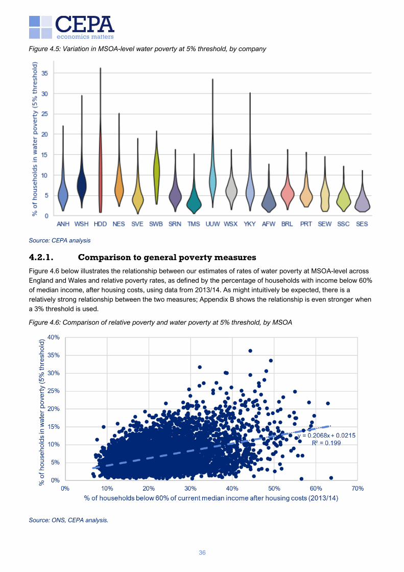
36

Figure 4.5: Variation in MSOA-level water poverty at 5% threshold, by company

Source: CEPA analysis

4.2.1. Comparison to general poverty measures

Figure 4.6 below illustrates the relationship between our estimates of rates of water poverty at MSOA-level across

England and Wales and relative poverty rates, as defined by the percentage of households with income below 60%

of median income, after housing costs, using data from 2013/14. As might intuitively be expected, there is a

relatively strong relationship between the two measures; Appendix B shows the relationship is even stronger when

a 3% threshold is used.

Figure 4.6: Comparison of relative poverty and water poverty at 5% threshold, by MSOA

Source: ONS, CEPA analysis.

37

Analysis from the University of York also suggests a close link between income poverty and water poverty. Data

from the Family Resources Survey 2018/19 shows that the majority of households in water poverty are also in

income poverty, but not all. Similarly, the majority of those in income poverty are in water poverty at the 3%

threshold, but only a minority at the 5% threshold. Table 4.3 illustrates the overlaps between the various measures

of income poverty (both relative and absolute) and water poverty.

Table 4.3: Overlap between income and water poverty

Measure of

income poverty

Income

poverty rate

% of households in water poverty

also in income poverty

% of households in income poverty

also in water poverty

3% threshold 5% threshold 3% threshold 5% threshold

Relative income

poverty*

21% 73% 92% 69% 37%

Absolute income

poverty**

9% 68% 91% 72% 40%

*Income below 60% of current median income. **Income below 60% of 2010/11 median income, held constant in real terms.

Source: Family Resources Survey 2018/19 analysis, Prof. Jonathan Bradshaw, Social Policy Research Unit, University of York.

4.3. THRESHOLD SENSITIVITY ANALYSIS

Our core analysis reflects common practice (both in the water sector and in the energy sector) of defining water

poverty based on a 3% or a 5% threshold of the bill to income ratio. Though our modelling approach does not allow

us to present detailed results of the distribution of households’ bill to income ratios, we have produced results using

a range of alternative thresholds (from 2% up to 7%) in order to inform a view of the sensitivity of the estimated

incidence of water poverty to changes in the threshold.

Figure 4.7 below shows the results, which suggest a non-linear relationship between the chosen threshold and the

incidence of water poverty at that threshold.

Figure 4.7: Regional water poverty incidence by bill to income ratio threshold

Source: CEPA analysis

38

5. INDICATIVE IMPACT OF INTERVENTIONS

In this section, we present analysis that explores the potential for our top-down methodology to be used in

estimating the impact of current interventions on water poverty from stakeholders in the water sector.

Interpretation of results

It is critical to understand the modelling context under which the results in this section have been estimated. This

will help to prevent inappropriate conclusions or policy implications being drawn. We emphasise the following

points to consider when interpreting the estimates:

• We do not consider the results of our analysis to reflect a ‘league table’ of companies. Water poverty is a

complex issue, and a number of key drivers are not necessarily within a company’s control.

• Our Guiding Principles call for a consistent, simple, and transparent approach across all companies. In

particular, we have applied a simplifying assumption regarding the targeting of current direct financial

support. More complex assumptions such as increasing the number of customer groups with different income

distributions would allow the estimates to capture more of the company-specific differences in support.

• Our indicative estimates for the impact of interventions consider the difference between pre- and post-

intervention water poverty. This will likely make them particularly sensitive to key assumptions. Further

work would need to be done to explore to what extent the ‘true’ impact of an intervention is augmented by

such residual model assumption effects. There is, however, reasonable theoretical evidence to suggest the

indicative estimates likely reflect a lower bound to the ‘true’ impact.

5.1. CONTEXT

In CEPA’s Phase One study for Water UK, we identified a range of interventions that companies currently apply to

those that are having trouble with their bills. These include:

• installing a water meter, potentially with a lowest price guarantee;

• advice on water use and water saving;

• benefits advice to maximise household income;

• social tariffs; and

• payments holidays or phasing of payments.

In principle, all of these could result in changes to the bill to income ratio, via either reducing bills or increasing

income (with the possible exception of phasing of payments).38 However, we do not currently have sufficient

information on all of these interventions to incorporate them fully into our modelling. The following analysis

therefore focuses on direct financial support to households.

Two key schemes applied across the England and Wales water sector are WaterSure and social tariffs. WaterSure

limits metered bills of eligible – low-income, high water use – customers to the average for the region. Companies

also offer social tariffs targeted at water poor customers, that are typically funded in part by cross-subsidising from

other customers’ bills.

CCW collates information on the approximate financial value of support currently offered by companies,

summarised in the table below.39

———————————————————————————————————————————————————

38 It is also important to acknowledge that such measures may have an impact on aspects of water poverty not captured within

the ‘strict’ definition of water poverty provided by a bill to income ratio. Payment holidays offers a salient example – while a

change in the due date of a bill may not effect the total charges faced, it can significantly improve a customer’s ability to manage

income volatility.

39 CCW, Nov 2020, Water for All: Water Affordability and Vulnerability Report 2019-20. Available here.

39

Table 5.1: Approximate WaterSure and social tariffs support, 2019/20

Company WaterSure Social tariffs

No. customers Approximate value No. customers Approximate value

Industry 166,946 £45.2 m 723,192 £105.5 m

Water and sewerage companies

Anglian Water 34,853 £8.8m 24,307 £4.3m

Dŵr Cymru 15,543 £2.2m 88,024 £24.4m

Hafren Dyfrdwy 847 £0.06m 872 £0.1m

Northumbrian Water* 8,130 £1.5m 30,624 £3.9m

Severn Trent Water 13,959 £2.8m 52,690 £11.7m

South West Water ** 13,403 £6.3m 12,218 £1.4m

Southern Water 13,856 £4.5m 84,373 £5.7m

Thames Water 13,836 £4.4m 150,372 £15.5m

United Utilities 22,772 £7.7m 68,552 £20.3m

Wessex Water 7,779 £2.2m 34,789 £4.7m

Yorkshire Water 7,205 £2.9m 19,795 £2.1m

Water-only companies

Affinity Water 4,055 £0.8m 60,230 £4.6m

Bristol Water 2,974 £0.4m 15,966 £1.3m

Hartlepool Water 320 £0.03m 559 £0.05m

Portsmouth Water 190 £0.01m 8,401 £0.2m

South East Water 5,220 £0.6m 33,575 £2.1m

South Staffs Water*** 1,763 £0.2m 23,534 £1.9m

SES Water 241 £0.06m 14,311 £1.4m

*Including Essex and Suffolk Water. **Including Bournemouth Water. ***Including Cambridge Water. Source: CCW40

When comparing the analysis in this section to these contextual numbers, we note our estimates are framed around

the 3% and 5% bill to income ratio thresholds defining water poverty. In particular, this means that any impact an

intervention has on a household if or once they are below the water poverty threshold will not be captured in our

estimates.

As our approach to measuring water poverty is new and being used on an industry-wide basis in this report for the

first time, current interventions were inevitably not designed or intended to maximise the reduction in water poverty

when measured using this approach, so this analysis should not be interpreted as an assessment of the

appropriateness of current interventions.

One implication is that, where the approximate total value of an intervention is broadly similar to the estimated value

up to the 3% or 5% threshold, it would suggest the targeting is, by coincidence, well aligned with the given

———————————————————————————————————————————————————

40 CCW note that this data is based on company assessments of the value of support delivered. As such these may be subject to

varying degrees of accuracy. In addition, CCW note that customers who are receiving help from both a water company and a water

and sewerage company may have been counted twice. CEPA has not confirmed the accuracy of this published data.

40

definition. However, should values not be similar, this is not necessarily evidence that an intervention is “failing”.

Rather, it may suggest that it is targeting aspects of water poverty not fully captured by a bill to income metric.41

We also note that financial support for households does not necessarily come solely from the companies. For

example, following the Walker Review into affordability in the water sector in 2009, the government committed to

contributing a £50 reduction to all bills in the South West. This currently remains in place.42

5.2. APPROACH TO ESTIMATION

For each of the four customer groups described in Section 2.3.1, the top-down methodology allows us to simulate

water poverty:

• pre-intervention – i.e., all customers face a form of standard charge, whether metered or unmetered; and

• post-intervention – i.e., once company interventions (e.g., social tariffs) are accounted for in the

simulation.

The analysis presented in Section 4 focused only on post-intervention water poverty, and so represents an estimate

for water poverty under current conditions. In order to explore what the extent of water poverty might have been in

the scenario where companies did not provide financial support to a subset of their customers, we can compare

water poverty metrics pre- and post-intervention.

The only difference between pre- and post-intervention estimates is that the latter uses ‘actual’ bill data to construct

the bill distribution, while the former uses ‘counterfactual’ data. Both actual and counterfactual data has been

provided by the water companies for the purposes of this analysis. A counterfactual bill is the bill that a discounted

customer would have received without the company intervention. This is reflected in Figure 5.1.

Figure 5.1: Overview of impact of intervention methodology

———————————————————————————————————————————————————

41 Another driver of differences would be the truncation approach of the four customer groups applied to our modelling (see

Section 0). This is a simplifying assumption that all companies use the same gross income eligibility criteria for their financial

support.

42 https://www.southwestwater.co.uk/bills/50-reduction/

41

By definition, counterfactual data will be more challenging to generate than the actual bills charged post-

intervention. Our initial analysis suggest a key challenge is calibrating assumptions to reflect diversity in company

water poverty strategies. Future analysis could focus on refining these assumptions to improve estimation of the

impact of company interventions.

There are a number of reasons why we would consider our approach to offer an estimate for the lower bound for

the impact of company interventions on water poverty. In general, any top-down methodology is more likely to

“miss” cases where an intervention has successfully brought a household out of water poverty than it is to

incorrectly identify households as brought out of water poverty when their bills remain unaffordable post-

intervention.

5.3. INITIAL ESTIMATES OF CURRENT COMPANY INTERVENTIONS

5.3.1. Maximal impact

Before more complex analysis is done, it is possible to conduct a high level illustration of the scope of current

company interventions to affect water poverty incidence. Table 5.2 sets out the numbers of households receiving

financial support, as given by the data provided to us from the companies. This is therefore also the maximum

number of households that could possibly be brought out of water poverty – defined using any bill to income

threshold – through companies’ current direct financial support.

Table 5.2: Customers receiving discounted bills from each company

Company No. of discounted customers43 Discounted customers as % of total customers

Industry 745,000 3.1%

Water and sewerage companies

Anglian Water 53,000 2.2%

Dwr Cymru 114,000 8.9%

Hafren Dyfrdwy 2,000 2.1%

Northumbrian Water 37,000 2.0%

Severn Trent Water 70,000 2.0%

South West Water 28,000 2.9%

Southern Water 57,000 4.5%

Thames Water 100,000 3.1%

United Utilities 82,000 3.0%

Wessex Water* 42,000 3.4%

Yorkshire Water 21,000 1.1%

Water-only companies

Affinity Water 52,000 4.2%

Bristol Water* 17,000 3.4%

Portsmouth Water 7,000 2.4%

South East Water 38,000 4.3%

South Staffs Water 27,000 4.0%

———————————————————————————————————————————————————

43 We note that the number of discounted customers as per data supplied to CEPA by companies (as per Table 5.2) is often

significantly different to the number of customers receiving financial support through WaterSure and social tariffs (as per Table

5.1). There are various potential reasons for this: for example, companies were given discretion as to which households should

be counted as ‘discounted’. We have taken company data submissions as given.

42

SES Water 15,000 5.3%

*Wessex Water and Bristol Water data provided jointly, so joint proportion of discounted customer assumed for both. Industry

total may not sum due to rounding. Source: CEPA analysis

For this impact to be reached, company interventions would have to be, by coincidence, “perfectly targeted”

against water poverty as defined in this study. In other words, every household provided with assistance would be

guaranteed to (1) have been defined as water poor pre-intervention, and (2) been moved to a bill to income ratio

below the poverty threshold post-intervention.

The analysis below relaxes this strong assumption to explore indicative estimates of what the impact of

interventions may have been in practice.

5.3.2. Pre- vs post-intervention water poverty

Analysis of the impact of water poverty interventions is more challenging to produce and interpret. In applying a

common, industry-wide approach to simulating water poverty we have necessarily applied a simplifying assumption

regarding the targeting of current direct financial support to simulated households.

Our results on intervention impacts – which are defined as the difference between water poverty incidence before

and after intervention – are particularly sensitive to modelling assumptions. Estimates produced using a common

industry-wide approach may not correspond precisely to companies' own estimates, which may be based on more

bespoke modelling approaches or input assumptions.

Nevertheless, our simulation results do give an indication of the impact of current interventions. Figure 5.2 displays

the bill to income ratios of households across England and Wales both pre- and -post intervention. Over 80% of

households typically have a bill to income ratio below either of the main definitions of water poverty. This highlights

that small changes in estimates for the remaining 20%, and in particular the change in values between pre- and

post-intervention, will mean results on the impact of intervention are particularly sensitive.

Figure 5.2: Estimated bill to income proportions pre- and post-intervention at industry level, 2019/20

Source: CEPA analysis

Table 5.3 summarises our impact of intervention estimates at the industry and region level. In the first column, we

estimate what water poverty (at the 5% bill-to-income threshold) would have been in the counterfactual scenario if

companies did not provide any financial discounts (i.e. all customers face a standard charge, whether metered or

unmetered). The remaining three columns reflect the difference between various measures in the post-intervention

scenario compared to the pre-intervention scenario: i.e., the reduction in the water poverty rate, the reduction in

total number of households above the 5% threshold, and the reduction in the total water poverty gap respectively.

There are a number of important points to note in interpreting the analysis in Table 5.3.

43

First, the estimated number of households moved below the applicable poverty threshold does not include

households whose bill to income ratio is reduced via company interventions, but remains above the 3% or 5%

threshold. Some households may be provided substantial financial support, but remain above the threshold due to

the extent of their pre-intervention water poverty. The impact on these households (up to and no further than the

3% or 5% threshold) is, however, captured in the reduction in the total water poverty gap.

For example, company support may reduce a household’s bill to income ratio from 8% to 6%, or from a 4.5% ratio

to 3.5%. Neither of these households would be included in the number of households moved below the poverty

threshold in our analysis, as neither has gone below the relevant threshold. However, the financial support provided

to them would be included in the reduction in the total water poverty gap. A consequence of this is that the number

of households estimated to move below the water poverty threshold in our analysis – as strictly defined in in this

report – is substantially below the number of households that are known to receive support from one of the two

main schemes in England and Wales, i.e., WaterSure and company social tariffs (see Table 5.1 above).

Finally there may be a degree of ‘overlap’ between the estimated reduction in households in water poverty at the

3% and 5% thresholds. For example, a household whose bill to income ratio is reduced from 6% to 2.5% would be

included in both the 3% and 5% estimate of households moved below the relevant water poverty threshold. It is also

not meaningful to consider the reduction in water poverty (£) per household taken out of water poverty in Table 5.3

(i.e. dividing “Reduction in total water poverty gap” by “Households moved below poverty threshold in water

poverty”), since different populations are considered for the two measures.

The full benefits of current interventions may be considered greater than indicated in Table 5.3. The findings in

Table 5.3 should be interpreted as technical estimates of the impacts of existing industry interventions within the

context of this study’s adopted definition of water poverty and modelling approach. They capture benefits defined

solely in terms of moving households below a particular water poverty threshold. Viewed from a broader

perspective, the interventions may help to reduce affordability pressures faced by water consumers in England and

Wales even where households concerned remain above the water poverty threshold.

Table 5.3: Estimated impact of interventions at 3% and 5% threshold by region

Region Pre-intervention

water poverty rate

Reduction in water

poverty rate from

interventions

Households moved

below poverty

threshold

Reduction in total

water poverty gap

3% threshold

Industry 18.9% -1.0% -226,000 -£131 m

England 18.2% -0.8% -179,000 -£103 m

Wales 30.8% -3.6% -47,000 -£28 m

5% threshold

Industry 7.6% -1.2% -263,000 -£89 m

England 7.3% -0.9% -203,000 -£72 m

Wales 13.4% -4.7% -61,000 -£17 m

Source: CEPA analysis

Figure 5.3 below sets out for each company the total water poverty gap reduction per discounted customer. This

can be interpreted as the average reduction in water poverty gap. However, this will mask significant variation in the

impact at a household level.

Estimates at a company level are even more sensitive to assumptions than the aggregate estimates above and, as

with all results in this section, should be considered indicative. These estimates will not necessarily correspond in

all cases to companies’ own analysis due to different methodologies.

In particular, differences will to some extent reflect that we have ensured a consistent approach is applied across

the industry. In contrast, company-specific analysis has more scope to make detailed assumptions that may not

necessarily be appropriate for a different company.

44

Figure 5.3: Reduction in total water poverty per discounted customer by company, 2019/20

Source: CEPA analysis

45

6. CONCLUSIONS AND NEXT STEPS

The results of this study demonstrate the feasibility of using a top-down simulation approach to estimating the

incidence of water poverty at the industry, regional and company level in England and Wales. We estimate an

overall industry-wide level of water poverty that is broadly consistent with previous studies. These estimates can be

replicated in order to consistently monitor water poverty over time. The results also show that there is considerable

variation in its incidence across the country – including large differences within and between supply areas. Any

interventions to address water poverty could therefore have quite different implications for customers, in addition to

existing variations in the degree of support provided.

Turning to policy implications, it is for the water sector to consider whether it wishes to adopt this approach as the

standard basis for assessing water poverty across England and Wales. If so, three particular issues would be

relevant:

• Targeting of support – which households should be defined as being in water poverty and requiring

support? How closely could (in theory) and should (in practice) support be targeted (or re-targeted in the

case of existing support schemes) to maximise the impact against the measure of water poverty used in

this study? This is particularly sensitive to the choice of water poverty threshold, with our analysis indicating

that around 11.5% of households across England and Wales fall between the 3% and 5% bill to income ratio

thresholds commonly used to define water poverty.

• Calibration of support – how much support do different households require, and how closely could (in

theory) and should (in practice) the level of support for a household be calibrated to maximise the impact

against the measure of water poverty used in this study? Our analysis indicates that at least a further

£236m would be required to eliminate water poverty at the 5% threshold, or £720m at the 3% threshold.

The actual value of support required would exceed this, however, assuming that it is not practical to

perfectly target and calibrate support. There is also an important challenge in valuing support that (a) may

move a household closer to but not beyond a given threshold, or (b) may be provided to a household that is

marginally outside the definition of water poverty but may still be in financially vulnerable circumstances.

• Funding of support. Though we have expressed the water poverty gap on a per non-water poor household

basis for illustrative purposes, in practice cross-subsidisation of water bills is only one potential policy

choice, and cross-subsidation could be carried out on an individual company basis, a regional basis or an

industry-wide basis. Our analysis – particularly that based on the lower 3% threshold for defining water

poverty – indicates that the implied support per non-water poor household may be substantial. Any further

interventions funded by bills may need to consider second-order impacts on water poverty as a result of

elevated standard tariffs.

Further analysis could help further inform these issues. The scope of the modelling could be further expanded and

refined to include more detailed data on the distribution of household-level water poverty, in addition to its

incidence at defined thresholds of the ratio of bills to income. More detailed analysis of the impact of interventions

would benefit from developing a more bespoke approach to assumptions on customer segmentation, income

distribution and the correlation between bills and income. Each of these refinements could be applied within the

framework of the simulation approach we have developed.

46

DETAILED METHODOLOGY

CONSTRUCTING BILL DISTRIBUTIONS

Assumptions in company data

Table A.1 details the assumptions made regarding data submissions received from each company. While we have

performed sense-checking and data cleaning to identify obvious errors, company data submissions were broadly

taken as given. In particular, companies performed their own calculations in order to estimate counterfactual data

for their discounted customers (i.e. what their bills would have been if they had not been receiving direct financial

support).

Table A.1: Assumptions made in company data

Company Acronym Comments on data

Water and sewerage companies

Anglian Water ANH Annualised bill data was based on a mix of 2019/20 and 2020/21 bills.

Data was provided in £20 intervals up to £1200. Households in the £1200-

£5000 interval provided by Anglian were distributed across the £20 intervals

between £1200 and £1500 assuming a uniform bill distribution between

£1200 and £5000. Following agreement with the company, we performed

two further adjustments to the data provided:

• The number of households with a bill above £1500 appeared erroneously

high, so these households were excluded from our analysis.

• For a significant proportion of WaterSure customers, distributional data on

counterfactual bills is not available (as consumption above the tariff cap is

not captured). We therefore apportioned the average counterfactual data

provided across the full distribution. The ‘excess’ households in the bill

interval of the average counterfactual bill (£820-£840) was interpolated

from the adjacent intervals. These excess customers were then

distributed across bill intervals above the WaterSure cap, in proportion to

the number of households already in those intervals.

Dŵr Cymru WSH Only customers in receipt of one of the company’s main social tariffs were

included as discounted. This does not include Water Direct or Water Collect

discounts, which assist around 15,000 customers a year.

Hafren Dyfrdwy HDD No sewerage-only bill distribution data was provided for LSOAs in the

Wrexham area. We used Dŵr Cymru’s aggregate sewerage bill distribution

data as a proxy for the sewerage bills received by Hafren Dyfrdwy’s water-

only households.

Only customers in receipt of a social tariff or on the WaterSure scheme

were counted as discounted.

Northumbrian Water NES Data submission includes Essex and Suffolk Water.

Severn Trent Water SVE Circa 5,000 properties with consumption above 500m3 excluded from data

submission by Severn Trent to remove erroneous bills and bulk supplies.

Only customers in receipt of a social tariff or on the WaterSure scheme

were counted as discounted.

South West Water SWB Data submission includes Bournemouth Water.

Bill data includes the £50 subsidy currently provided by the government on

bills in the South West region.

Southern Water SRN No additional assumptions.

Thames Water TMS No additional assumptions.

United Utilities UUW No additional assumptions.

Wessex Water WSX Data was provided in joint submission with Bristol Water.

47

Number of households served by BRL and WSX respectively in each LSOA

was provided separately.

Yorkshire Water YKY No additional assumptions.

Water-only companies

Affinity Water AFW No additional assumptions.

Bristol Water BRL Data was provided in joint submission with Wessex Water.

Number of households served by BRL and WSX respectively in each LSOA

was provided separately.

Portsmouth Water PRT No additional assumptions.

South East Water SEW No additional assumptions.

South Staffs Water SSC Data submission included Cambridge Water.

No additional assumptions.

SES Water SES Data was provided at a property and bill-payment level. We applied the

following assumptions in order to transform this data into a format consistent

with other companies’ submissions:

• Only bill payments that took place during 2019/20 were considered. The

sum of bills (or credit payments) associated with a property reference was

used to calculate the annualised bill. This includes cases where accounts

were closed and a new account opened at the same property within the

year.

• In cases where bills for the same property have categorised the property

as both ‘metered’ and ‘unmetered’, we assume the characteristic of the

earlier bill.

• Geographical data is only available to the Local Authority level, a higher

level of aggregation than MSOA. We assume the company has customers

in all MSOAs of the Local Authority, and that these households are spread

evenly across the MSOAs in the region.

Processing of bill distribution data

Table A.2 details the steps taken to process company data submissions (post reformatting where necessary) into a

workable database for input into our simulation model.

Table A.2: Stages, rationale and detail of bill distribution processing

Stage Rationale Inputs Processing

Aggregate

company

data to

MSOA-

level

As discussed in

Section 2.2.3, we

have chosen to

undertake analysis at

MSOA-level. This

requires aggregation

of company

submissions (which

were provided at

LSOA-level).

Bill distribution data at

LSOA-level, separated by:

• company;

• service type (combined,

water-only or sewerage-

only); and

• bill type (metered standard

actual (MSA), unmetered

standard actual (USA),

metered discounted actual

(MDA), unmetered

discounted actual (UDA),

metered discounted

counterfactual (MDC), or

unmetered discounted

counterfactual (UDC)).

For each dataset:

• Aggregate data from LSOA- to MSOA-

level.

• Distribute any households in the ‘Non-

Allocated’ row (i.e., not assigned to a

specific MSOA) across all MSOA

served by that company.

Aggregate

companies

We calculate water

poverty rates for

Bill distribution data at

MSOA-level, separated by:

For each service type and bill type:

48

each MSOA, which

requires combining

all company data

together to cover all

of England and

Wales.

• company;

• service type (combined,

water-only, or sewerage-

only); and

• bill type (MSA, USA, MDA,

UDA, MDC or UDC).

• Append all corresponding company

files into one dataset, creating variables

to indicate the number of households

served by each company in each

MSOA.

• Consolidate data to obtain one row of

data per MSOA.

Combine

metered

and

unmetered

sewerage

bill data

Our model requires a

dataset of combined

bill distributions for

each MSOA in

England and Wales,

thus water- and

sewerage-only bill

data must be

combined. To avoid

making an

assumption on

whether a household

with a metered water

supply has a

metered or

unmetered sewerage

connection, we

combine metered

and unmetered

sewerage bill data

together into a single

bill distribution,

which is then used to

combine with water-

only bill data.

Sewerage-only bill

distribution data covering all

MSOAs across England and

Wales, separated by bill type

(MSA, USA, MDA, UDA,

MDC or UDC).

For context, households with

separate providers for water

and sewerage services

comprise approximately 10%

of all households.

The following categories are combined

for sewerage-only bill data:

• Metered / unmetered standard actual

becomes standard actual (SA).

• Metered / unmetered discounted actual

becomes discounted actual (DA).

• Metered / unmetered discounted

counterfactual becomes discounted

counterfactual (DC).

Combine

water- and

sewerage-

only bill

data

As discussed above,

our model requires a

dataset of combined

(water and

sewerage) bill

distributions for each

MSOA in England

and Wales, thus

water- and

sewerage-only bill

data must be

combined.

Water-only bill distribution

data covering all MSOAs

across England and Wales,

separated by bill type (MSA,

USA, MDA, UDA, MDC or

UDC).

Sewerage-only bill

distribution data covering all

MSOAs across England and

Wales, separated by bill type

(SA, DA, or DC).

For each water-only bill type and

corresponding sewerage-only bill type

(e.g., metered discounted actual water-

only bill data and discounted actual

sewerage-only bill data):

• Transform distribution data from

number of households into proportions.

• Split each bill interval in two to give

£10 bill intervals, assuming equal

frequency in each44.

• Assuming a perfect correlation

between water and sewerage bills45,

calculate the proportion of households

in each combined bill interval, following

the algorithm in Figure A.1.

• N.B., households with a discounted

water bill are assumed to have a

———————————————————————————————————————————————————

44 This aids with the subsequent calculation of combined bills by ensuring that the sum of two interval midpoints is not on the

boundary between two intervals. For example, using £20 intervals, the sum of the midpoints of the £100-£120 water-only bill

interval and the £120-£140 sewerage-only bill interval gives £110 + £130 = £240 which is on the boundary of the £220-£240 and

£240-£260 combined bill intervals. By contrast, the midpoints of £10 intervals, e.g. £105 + £125 = £130 is in the middle of the

£120-£140 combined bill interval.

45 That is, a household that has a water-only bill at a certain point of the water-only bill distribution (e.g., the 35th percentile),

would have a sewerage-only bill at the same point of the sewerage-only bill distribution.

49

discounted sewerage bill. If there is no

discounted sewerage bill data for an

MSOA, standard data is used instead.

• Recombine £10 bill intervals into £20

intervals and transform the data back

into numbers of households.

Combine

all data

Water- and

sewerage-only bill

data that has been

combined in the

previous step is

combined with bill

data which was

submitted by

companies as

combined, to provide

an overall combined

bill distribution for

input into the model.

Combined bill distribution

data covering all MSOAs

across England and Wales,

separated by:

• bill type (MSA, USA, MDA,

UDA, MDC, or UDC);

• bill data submitted by

companies as combined;

and

• water- and sewerage-only

bill data combined as per

the previous step.

For each bill type:

• Append the bill distribution data

combined as per the previous step with

the corresponding bill distribution data

which was submitted by companies as

combined.

• Consolidate the data to obtain one row

of data per MSOA.

Calculate

total

households

served by

each

company

in each

MSOA

Company totals are

required to weight

MSOA-level water

poverty rates to

calculate company-

level poverty rates.

Total households served by

each company, separated

by:

• service type (combined,

water-only, or sewerage-

only); and

• bill type (MSA, USA, MDA,

UDA, MDC or UDC).

• Only households in ‘actual’ data

submissions are counted (as the same

households feature in discounted

actual and discounted counterfactual

data submissions)

• All service types are counted, to

properly reflect the number of

households served by each company.

This means that the sum of company

totals will not equal the total number of

households overall, as counting both

water- and sewerage-only households

will entail some double counting,

assuming that households generally

receive both water and sewerage

services.

50

Figure A.1: Algorithm to combine water- and sewerage-only bill distributions

Algorithm to combine water- and sewerage-only bill distributions

In effect, this algorithm walks through the water-only bill distribution, considering each household in turn and

finding its corresponding sewerage-only bill, and combining this with the water-only bill to calculate a combined

bill.

For each MSOA:

1. Let each £10 bill interval be numbered, starting at 0 and ending at 149 (from £0-£10, to £1,490-

£1,500).

2. Define (i, j) = (0, 0) and define the ‘combined list’ as a list where each entry gives the proportion of

households in a specific water-only bill interval and a specific (potentially different) sewerage-only bill

interval.

3. Compare the proportions of households in water-only bill interval i and sewerage-only bill interval j.

If there are fewer households in the water-only bill interval i than sewerage-only bill interval j, then:

o Add the proportion of households in water-only bill interval i to the ‘combined list’, linked to

water-only bill interval i and sewerage-only bill interval j.

o Subtract the proportion of households in the water-only bill interval i from the proportion of

households in sewerage-only bill interval j.

o Add 1 to i.

Else:

o Add the proportion of households in sewerage-only bill interval j to the ‘combined list’, linked to

water-only bill interval i and sewerage-only bill interval j.

o Subtract the proportion of households in the sewerage-only bill interval j from the proportion of

households in water-only bill interval i.

o Add 1 to j.

4. Repeat step 3 until (i, j) = (149, 149)

51

SIMULATION MODELLING ASSUMPTIONS

Table A.3: Baseline model parameters

Parameter Baseline value Explanation / Justification

‘Targeting’ assumptions

Bill to income

threshold

definition

3% and 5% Common practice in regulated sectors uses these thresholds. Ofwat’s

‘Affordability and debt 2014-15’ report is an early example which refers

to the proportion of households spending more than 3% or 5% of their

income on water and sewerage bills.46

Identification

of

‘discounted’

customers

Company input Given their knowledge of their own charging structures and our broad

definition of a ‘discounted’ customer, companies are best placed to

determine which customers should be classified as such.

Distributional assumptions

Truncation

threshold

£19,201 in London

£16,105 elsewhere

A group of companies in the South of England (Southern, South East,

SES, Affinity, and Thames) have aligned their social tariff eligibility

criteria to an income threshold based on the standard HMRC Low

Income Threshold for a number of means-tested benefits. For London

residents, the group of companies use a higher threshold based on the

annualised equivalent based on a 35-hour week, as calculated by the

London Living Wage Foundation.

These are gross unequivalised income values, which includes all

income, benefits and allowances (excluding disability related

payments). In our modelling we adjust this £11,274 (£13,441 for

London MSOAs) to be consistent with our income definition.

Bill-income

correlation

Metered: 0.05

Unmetered: 0.10

Based on correlation analysis described below.

Absolute

minimum

income

£4,000 This is marginally less than the minimum annual Universal Credit

Standard allowance of £4,112.64 for a single individual under the age

of 25.47

Maximum bill

multiplier

1.00 relative to

£1,500

Although some households may have annual water and sewerage

charges greater than £1,500 this is a small proportion. Most data points

above this point are likely to be incorrectly labelled non-domestic

customers or bulk billing sites with multiple households. We therefore

assume a charge of exactly £1,500 for any data points provided in the

‘£1,500+’ interval in company data.

Boundary

income

multiplier

‘Low’ distribution:

min 0.00 relative to

5th percentile

‘Residual’

distribution: min 0.50

relative to 5th perc.;

max 1.00 relative to

95th perc.

The national level income distribution provides relative incomes

according to the mid-point of the ten deciles of the population.

Therefore is it necessary to define the maximum and minimum possible

incomes (i.e. the 0th and 100th percentiles of the distribution).

The minimum is assumed to be £0 for those in the ‘low’ distribution

(noting this will be ratcheted up to the absolute minimum income

defined above). For those based on the ‘residual’ distribution, we would

expect less chance of a household having an extremely low income.

All simulated households above the 95th percentile income are

modelled using the 95th percentile value (noting these cases are less

critical when exploring water poverty more associated with lower

income households).

———————————————————————————————————————————————————

46 Ofwat, December 2015. Affordability and debt 2014-15 – supporting information. Available here.

47 UK Government. Universal Credit – What you’ll get. Available here.

52

Model construction

Treatment of

disability

payments

Within simulation DWP data on the incidence and size of Personal Independence

Payments across England and Wales is used to adjust the simulatated

income of a proportion of hypothetical households. This accounts for

the fact that disability allowances should not be included in the

disposable income considered in the bill to income ratio.

Simulation

per MSOA

customer

group

1,000 The greater the number of hypothetical households generated, the

more precise our estimates will be. One thousand simulations per

group per MSOA is an arbitrary parameter that balances precision with

computational requirements.

Minimum

households

for MSOA

estimation

50 Estimates are not produced where the there are fewer than 50 bill data

points available. Where the sample size is small, the bill distribution

produced will not be robust enough to reliably proxy the ‘actual’

distribution. Although an arbitrary rule of thumb, a sample size of

greater than around 30 is often offered as a level at which typical

statistical assumptions begin to reasonably hold.

Correlation analysis

Our assumptions regarding the correlation between household income and water and sewerage bills were informed

using analysis of the 2018-2019 Family Resources Survey data. Table A.4 below gives the Pearson correlation

coefficients between equivalised net household income after housing costs (but before water and sewerage

payments) and household water and sewerage bills, by region. The Pearson correlation coefficient is a measure of

the strength of the linear relationship between two variables, and can take values between -1 and +1. Values of -1

and +1 corresponds to data points lying exactly on a straight line with a negative and positive gradient, respectively,

while a value of 0 means there is no linear relationship between the variables.

The figures in the table below show that there is a weakly positive relationship between household income and

water and sewerage bills. There is also considerable variation in the bill-income correlation across regions.

However, for the sake of consistency and parsimony, we choose to use a correlation coefficient of 0.05 and 0.10 for

metered and unmetered households, respectively, across all regions, based on the correlation coefficients for

England and Wales.

Table A.4: Pearson correlation coefficients between household income and water and sewerage bills, by region

Region Metered Unmetered

North East -0.06 0.22

North West and Merseyside 0.01 0.17

Yorkshire and Humberside 0.04 0.13

East Midlands 0.02 0.11

West Midlands 0.09 0.13

Eastern 0.00 0.06

London 0.02 0.12

South East 0.01 0.10

South West 0.07 0.08

Wales 0.09 0.08

England and Wales 0.03 0.10

Source: Family Resources Survey 2018/19, Prof. Jonathan Bradshaw, Social Policy Research Unit, University of York.

53

DATA SOURCES

Table A.5: Summary of data sources used

Data Source Use in analysis

Water and sewerage bill

distributions

Company data For compiling bill distributions covering

MSOAs across England and Wales.

National income

distribution

ONS, Effects of taxes and benefits

on household income (June 2020)

To inform the 'shape' of income distributions

at MSOA level.

MSOA-level average

income

ONS, Income estimates for small

areas (March 2020)

To adjust the national income distribution to

reflect incomes in each MSOA.

Personal Independence

Payment (PIP)

DWP Stat-Xplore PIP cases with

entitlement (March 2020)

To adjust income distributions to remove

disability benefits.

Geospatial data ONS Open Geography Geoportal Construction of map outputs

Relative poverty rates by

MSOA

ONS, Households in poverty

estimates for middle layer super

output areas in England and

Wales. Model-based estimated of

the proportion of households with

mean weekly income lower than

60% of national median weekly

income. (2013/14)

For comparative analysis with estimated

water poverty rates.

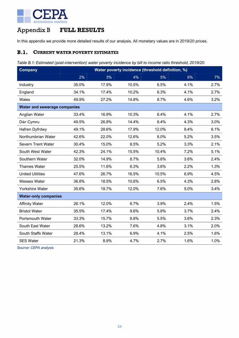
54

FULL RESULTS

In this appendix we provide more detailed results of our analysis. All monetary values are in 2019/20 prices.

CURRENT WATER POVERTY ESTIMATES

Table B.1: Estimated (post-intervention) water poverty incidence by bill to income ratio threshold, 2019/20

Company Water poverty incidence (threshold definition, %)

2% 3% 4% 5% 6% 7%

Industry 35.0% 17.9% 10.5% 6.5% 4.1% 2.7%

England 34.1% 17.4% 10.2% 6.3% 4.1% 2.7%

Wales 49.9% 27.2% 14.8% 8.7% 4.6% 3.2%

Water and sewerage companies

Anglian Water 33.4% 16.9% 10.3% 6.4% 4.1% 2.7%

Dŵr Cymru 49.5% 26.8% 14.4% 8.4% 4.3% 3.0%

Hafren Dyfrdwy 49.1% 28.6% 17.9% 12.0% 8.4% 6.1%

Northumbrian Water 42.6% 22.0% 12.6% 8.0% 5.2% 3.5%

Severn Trent Water 30.4% 15.0% 8.5% 5.2% 3.3% 2.1%

South West Water 42.3% 24.1% 15.5% 10.4% 7.2% 5.1%

Southern Water 32.0% 14.9% 8.7% 5.6% 3.6% 2.4%

Thames Water 25.5% 11.6% 6.3% 3.6% 2.2% 1.3%

United Utilities 47.6% 26.7% 16.5% 10.5% 6.9% 4.5%

Wessex Water 36.8% 18.5% 10.6% 6.5% 4.3% 2.8%

Yorkshire Water 35.6% 19.7% 12.0% 7.6% 5.0% 3.4%

Water-only companies

Affinity Water 26.1% 12.0% 6.7% 3.9% 2.4% 1.5%

Bristol Water 35.5% 17.4% 9.6% 5.8% 3.7% 2.4%

Portsmouth Water 33.3% 15.7% 8.8% 5.5% 3.6% 2.3%

South East Water 28.6% 13.2% 7.6% 4.8% 3.1% 2.0%

South Staffs Water 28.4% 13.1% 6.9% 4.1% 2.5% 1.6%

SES Water 21.3% 8.9% 4.7% 2.7% 1.6% 1.0%

Source: CEPA analysis

55

Table B.2: Estimated (post-intervention) water poverty gap by bill to income ratio threshold, 2019/20

Company Total water poverty gap, £ millions (by threshold definition, %)

2% 3% 4% 5% 6% 7%

Industry £1,492.4 m £719.8 m £396.4 m £235.6 m £147.3 m £95.3 m

England £1,368.2 m £662.7 m £368.0 m £219.9 m £137.5 m £88.9 m

Wales £124.2 m £57.0 m £28.4 m £15.7 m £9.8 m £6.4 m

Water and sewerage companies

Anglian Water £156.9 m £76.1 m £42.6 m £25.6 m £16.1 m £10.4 m

Dŵr Cymru £118.2 m £53.3 m £25.9 m £14.0 m £8.5 m £5.5 m

Hafren Dyfrdwy £12.5 m £6.9 m £4.2 m £2.7 m £1.8 m £1.3 m

Northumbrian Water £145.1 m £68.5 m £37.4 m £22.2 m £13.6 m £8.6 m

Severn Trent Water £169.0 m £78.7 m £42.4 m £24.6 m £14.9 m £9.2 m

South West Water £116.5 m £65.1 m £39.9 m £25.8 m £17.5 m £12.2 m

Southern Water £70.9 m £32.4 m £18.0 m £10.8 m £6.7 m £4.2 m

Thames Water £133.0 m £58.2 m £30.0 m £16.8 m £9.9 m £6.0 m

United Utilities £271.2 m £139.3 m £78.9 m £47.5 m £29.9 m £19.6 m

Wessex Water £90.5 m £43.0 m £23.5 m £14.0 m £8.8 m £5.7 m

Yorkshire Water £138.5 m £71.3 m £40.8 m £25.0 m £16.2 m £10.8 m

Water-only companies

Affinity Water £50.0 m £21.5 m £11.0 m £6.1 m £3.6 m £2.1 m

Bristol Water £32.9 m £15.0 m £7.9 m £4.6 m £2.8 m £1.7 m

Portsmouth Water £16.4 m £7.3 m £3.9 m £2.3 m £1.4 m £0.8 m

South East Water £47.1 m £20.7 m £11.2 m £6.7 m £4.1 m £2.6 m

South Staffs Water £27.7 m £12.1 m £6.3 m £3.5 m £2.1 m £1.3 m

SES Water £9.0 m £3.7 m £1.8 m £1.0 m £0.6 m £0.3 m

Note: Company values may not add up to country level aggregates due to households with separate water and sewerage

providers. Source: CEPA analysis

56

Table B.3: Estimated (post-intervention) water poor households by bill to income ratio threshold, 2019/20

Company Total estimated households in water poverty (by threshold definition, %)

2% 3% 4% 5% 6% 7%

Industry 7,926,000 4,066,000 2,371,000 1,468,000 935,000 618,000

England 7,276,000 3,712,000 2,178,000 1,354,000 875,000 577,000

Wales 650,000 354,000 192,000 114,000 60,000 42,000

Water and sewerage companies

Anglian Water 793,000 401,000 244,000 152,000 99,000 65,000

Dŵr Cymru 635,000 344,000 185,000 108,000 55,000 38,000

Hafren Dyfrdwy 47,000 27,000 17,000 11,000 8,000 6,000

Northumbrian Water 803,000 415,000 238,000 151,000 98,000 66,000

Severn Trent Water 1,041,000 515,000 291,000 177,000 112,000 72,000

South West Water 415,000 236,000 152,000 102,000 71,000 50,000

Southern Water 402,000 187,000 110,000 70,000 46,000 30,000

Thames Water 825,000 377,000 204,000 118,000 70,000 43,000

United Utilities 1,308,000 734,000 453,000 287,000 190,000 125,000

Wessex Water 449,000 226,000 129,000 80,000 52,000 34,000

Yorkshire Water 686,000 379,000 231,000 146,000 96,000 65,000

Water-only companies

Affinity Water 322,000 149,000 82,000 48,000 30,000 19,000

Bristol Water 179,000 88,000 48,000 29,000 19,000 12,000

Portsmouth Water 99,000 47,000 26,000 16,000 11,000 7,000

South East Water 251,000 115,000 66,000 42,000 27,000 18,000

South Staffs Water 191,000 88,000 46,000 27,000 17,000 11,000

SES Water 60,000 25,000 13,000 8,000 5,000 3,000

Note: Company values may not add up to country level aggregates due to households with separate water and sewerage

providers. Source: CEPA analysis

57

Table B.4: Estimated (post-intervention) gap per water poor household by bill to income ratio threshold, 2019/20

Company Water poverty gap per water poor household (by threshold definition, %)

2% 3% 4% 5% 6% 7%

Industry £188 £177 £167 £161 £158 £154

England £188 £179 £169 £162 £157 £154

Wales £191 £161 £148 £138 £163 £153

Water and sewerage companies

Anglian Water £198 £190 £175 £168 £163 £160

Dŵr Cymru £186 £155 £140 £129 £154 £144

Hafren Dyfrdwy £269 £254 £247 £239 £228 £219

Northumbrian Water £181 £165 £157 £147 £138 £131

Severn Trent Water £162 £153 £146 £139 £133 £127

South West Water £281 £276 £263 £253 £247 £244

Southern Water £177 £173 £164 £155 £146 £142

Thames Water £161 £154 £147 £143 £141 £140

United Utilities £207 £190 £174 £165 £158 £157

Wessex Water £201 £190 £183 £176 £169 £165

Yorkshire Water £202 £188 £177 £172 £169 £166

Water-only companies

Affinity Water £155 £145 £134 £128 £118 £111

Bristol Water £183 £170 £163 £156 £149 £142

Portsmouth Water £166 £156 £150 £139 £127 £117

South East Water £188 £180 £169 £159 £152 £146

South Staffs Water £145 £138 £135 £129 £124 £119

SES Water £150 £146 £138 £132 £129 £128

Source: CEPA analysis

58

Table B.5: Estimated (post-intervention) gap per non-water poor household by bill to income ratio threshold,

2019/20

Company Water poverty gap per non-water poor household (by threshold definition, %)

2% 3% 4% 5% 6% 7%

Industry £103 £39 £20 £11 £7 £4

England £99 £38 £19 £11 £7 £4

Wales £190 £60 £26 £13 £8 £5

Water and sewerage companies

Anglian Water £99 £39 £20 £12 £7 £5

Dŵr Cymru £182 £57 £24 £12 £7 £4

Hafren Dyfrdwy £259 £102 £54 £32 £21 £14

Northumbrian Water £134 £47 £23 £13 £8 £5

Severn Trent Water £71 £27 £14 £8 £4 £3

South West Water £206 £87 £48 £29 £19 £13

Southern Water £83 £30 £16 £9 £6 £3

Thames Water £55 £20 £10 £5 £3 £2

United Utilities £188 £69 £34 £19 £12 £7

Wessex Water £117 £43 £22 £12 £8 £5

Yorkshire Water £112 £46 £24 £14 £9 £6

Water-only companies

Affinity Water £55 £20 £10 £5 £3 £2

Bristol Water £101 £36 £17 £10 £6 £4

Portsmouth Water £83 £29 £14 £8 £5 £3

South East Water £75 £27 £14 £8 £5 £3

South Staffs Water £58 £21 £10 £5 £3 £2

SES Water £41 £14 £7 £4 £2 £1

Source: CEPA analysis

59

Figure B.1: MSOA-level (post-intervention) water poverty at 5% threshold

Source: CEPA analysis

60

Figure B.2: MSOA-level (post-intervention) water poverty at 3% threshold

Source: CEPA analysis

61

Figure B.3: Variation in MSOA-level water poverty at 5% threshold, by company

Source: CEPA analysis

Figure B.4: Variation in MSOA-level water poverty at 3% threshold, by company

Source: CEPA analysis

62

Figure B.5: Comparison of relative poverty and water poverty at 5% threshold, by MSOA

Source: ONS, CEPA analysis.

Figure B.6: Comparison of relative poverty and water poverty at 3% threshold, by MSOA

Source: ONS, CEPA analysis.

63

IMPACT OF INTERVENTION ESTIMATES

Table B.6: Estimated impact of interventions at 5% threshold

Company Pre-

intervention

water poverty

rate

Reduction in

water poverty

rate from

interventions

Households

moved below

poverty

threshold

Reduction in

total water

poverty gap

Reduction in

total gap per

discounted hh

Industry 7.6% -1.2% -263,000 -£88.6 m -£119

England 7.3% -0.9% -203,000 -£71.8 m -£114

Wales 13.4% -4.7% -61,000 -£16.8 m -£145

Water and sewerage companies

Anglian Water 7.5% -1.1% -27,000 -£13.1 m -£247

Dŵr Cymru 13.3% -4.8% -62,000 -£17.2 m -£151

Hafren Dyfrdwy 12.4% -0.5% 0 -£0.1 m -£40

Northumbrian Water 8.8% -0.8% -15,000 -£4.5 m -£123

Severn Trent Water 6.1% -1.0% -33,000 -£6.9 m -£98

South West Water 11.1% -0.7% -7,000 -£6.8 m -£247

Southern Water 6.5% -1.0% -12,000 -£5.6 m -£97

Thames Water 4.5% -0.9% -29,000 -£5.2 m -£52

United Utilities 11.9% -1.4% -39,000 -£14.2 m -£173

Wessex Water 7.5% -1.0% -12,000 -£3.5 m -£83

Yorkshire Water 8.0% -0.5% -9,000 -£5.5 m -£262

Water-only companies

Affinity Water 5.2% -1.3% -16,000 -£4.7 m -£91

Bristol Water 7.3% -1.5% -8,000 -£1.8 m -£102

Portsmouth Water 6.0% -0.5% -1,000 -£0.4 m -£57

South East Water 5.7% -0.9% -8,000 -£4.1 m -£110

South Staffs Water 4.2% -0.2% -1,000 -£0.1 m -£2

SES Water 2.9% -0.2% -1,000 -£0.1 m -£8

Source: CEPA analysis

64

Table B.7: Estimated impact of interventions at 3% threshold

Company Pre-

intervention

water poverty

rate

Reduction in

water poverty

rate from

interventions

Households

moved below

poverty

threshold

Reduction in

total water

poverty gap

Reduction in

total gap per

discounted hh

Industry 18.9% -1.0% -226,000 -£130.6 m -£175

England 18.2% -0.8% -179,000 -£102.8 m -£164

Wales 30.8% -3.6% -47,000 -£27.8 m -£239

Water and sewerage companies

Anglian Water 17.4% -0.6% -14,000 -£15.8 m -£298

Dŵr Cymru 30.6% -3.7% -48,000 -£28.4 m -£249

Hafren Dyfrdwy 29.2% -0.6% -1,000 -£0.2 m -£77

Northumbrian Water 22.7% -0.7% -14,000 -£7.1 m -£194

Severn Trent Water 16.5% -1.5% -50,000 -£13.0 m -£185

South West Water 24.5% -0.4% -3,000 -£7.6 m -£273

Southern Water 15.3% -0.4% -5,000 -£7.0 m -£122

Thames Water 13.0% -1.3% -44,000 -£11.5 m -£116

United Utilities 27.5% -0.8% -22,000 -£19.3 m -£236

Wessex Water 19.3% -0.9% -10,000 -£5.3 m -£126

Yorkshire Water 19.7% 0.0% 0 -£6.2 m -£297

Water-only companies

Affinity Water 13.1% -1.1% -13,000 -£7.6 m -£145

Bristol Water 19.0% -1.6% -8,000 -£3.0 m -£175

Portsmouth Water 15.9% -0.2% -1,000 -£0.6 m -£92

South East Water 13.5% -0.4% -3,000 -£5.1 m -£135

South Staffs Water 13.8% -0.7% -5,000 -£0.4 m -£15

SES Water 9.2% -0.3% -1,000 -£0.2 m -£16

Source: CEPA analysis

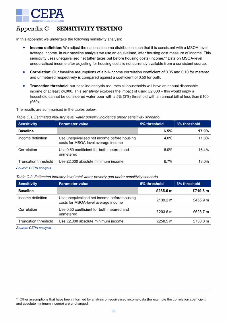
65

SENSITIVITY TESTING

In this appendix we undertake the following sensitivity analysis:

• Income definition: We adjust the national income distribution such that it is consistent with a MSOA-level

average income. In our baseline analysis we use an equivalised, after housing cost measure of income. This

sensitivity uses unequivalised net (after taxes but before housing costs) income.48 Data on MSOA-level

unequivalised income after adjusting for housing costs is not currently available from a consistent source.

• Correlation: Our baseline assumptions of a bill-income correlation coefficient of 0.05 and 0.10 for metered

and unmetered respectively is compared against a coefficient of 0.50 for both.

• Truncation threshold: our baseline analysis assumes all households will have an annual disposable

income of at least £4,000. This sensitivity explores the impact of using £2,000 – this would imply a

household cannot be considered water poor with a 5% (3%) threshold with an annual bill of less than £100

(£60).

The results are summarised in the tables below.

Table C.1: Estimated industry level water poverty incidence under sensitivity scenario

Sensitivity Parameter value 5% threshold 3% threshold

Baseline 6.5% 17.9%

Income definition Use unequivalised net income before housing

costs for MSOA-level average income

4.0% 11.8%

Correlation Use 0.50 coefficient for both metered and

unmetered

6.0% 16.4%

Truncation threshold Use £2,000 absolute minimum income 6.7% 18.0%

Source: CEPA analysis

Table C.2: Estimated industry level total water poverty gap under sensitivity scenario

Sensitivity Parameter value 5% threshold 3% threshold

Baseline £235.6 m £719.8 m

Income definition Use unequivalised net income before housing

costs for MSOA-level average income £139.2 m £455.9 m

Correlation Use 0.50 coefficient for both metered and

unmetered £203.6 m £628.7 m

Truncation threshold Use £2,000 absolute minimum income £250.5 m £730.0 m

Source: CEPA analysis.

———————————————————————————————————————————————————

48 Other assumptions that have been informed by analysis on equivalised income data (for example the correlation coefficient

and absolute minimum income) are unchanged.

UK

Queens House

55-56 Lincoln’s Inn Fields

London WC2A 3LJ

T. +44 (0)20 7269 0210

E. info@cepa.co.uk

www.cepa.co.uk

Australia

Level 20, Tower 2 Darling Park

201 Sussex St

Sydney NSW2000

T. +61 2 9006 1307

E. info@cepa.net.au

www.cepa.net.au