SAMPLING AND ESTIMATION

2

PARAMETERS AND STATISTICS

• A parameter is a quantity used to describe a population, and a statistic is a quantity computed from a sample and is used to estimate a population parameter and describe the sample.

- We typically use statistics to estimate parameters because

1. It isn’t possible to examine the entire population.

2. It isn’t feasible to examine the entire population (e.g., too expensive).

- In order for a calculated statistic to convey information about the related population parameter, certain conditions must be met; those conditions are generally satisfied if the sample used to calculate the statistics is random.

3

RANDOM SAMPLES

A simple random sample is a subset of the population drawn in such a way that each element of the population has an equal probability of being selected.

• The key to random sampling lies in the lack of any patterns in the collection of the data elements.

- Finite and limited populations can be sampled by assigning random numbers to all of the elements in the population, and then selecting the sample elements by using a random number generator and matching the generated numbers to the assigned numbers.

If you can enumerate the population, why don’t you just use it?

- When we can’t identify all the members of the population, we often use kth member sampling, where we select every kth member we observe until we have the necessary sample size.

Survey Prediction: Alfred Landon wins over FDR with 57% of the vote to 43% of the vote.

– Literary Digest, 1936

4

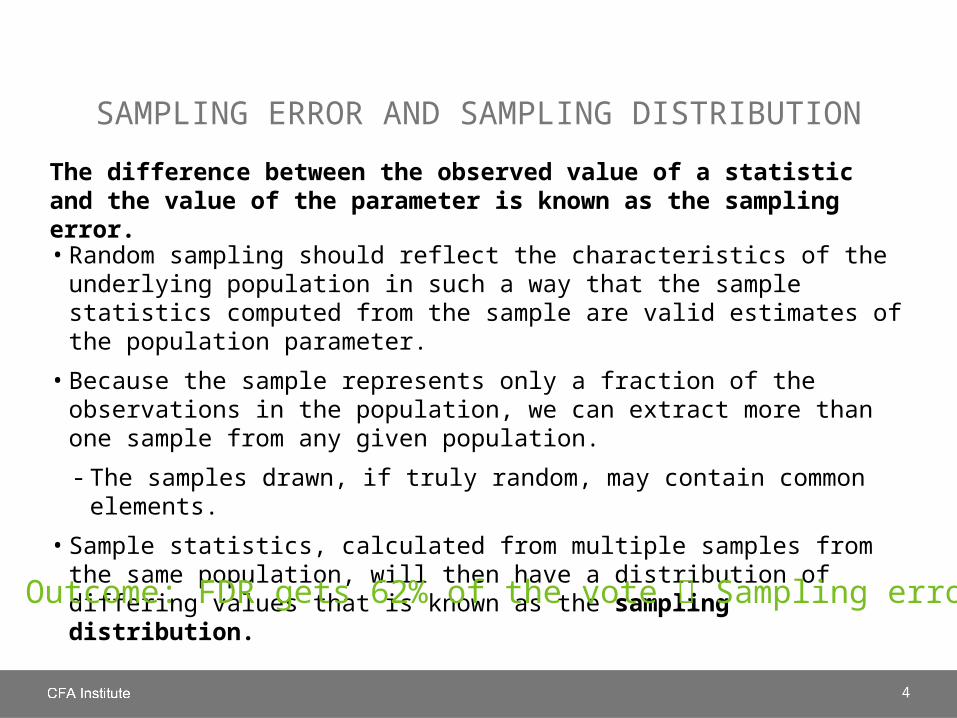
SAMPLING ERROR AND SAMPLING DISTRIBUTION

The difference between the observed value of a statistic and the value of the parameter is known as the sampling error.

• Random sampling should reflect the characteristics of the underlying population in such a way that the sample statistics computed from the sample are valid estimates of the population parameter.

• Because the sample represents only a fraction of the observations in the population, we can extract more than one sample from any given population.

- The samples drawn, if truly random, may contain common elements.

• Sample statistics, calculated from multiple samples from the same population, will then have a distribution of differing values that is known as the sampling distribution.

Outcome: FDR gets 62% of the vote Sampling error was 19%!

5

SAMPLING DISTRIBUTION

The distribution of possible outcomes of a sample statistic that would result from repeated sampling from the population.

• The samples drawn from the population to derive the distribution should be the same size and drawn from the same underlying population.

• We generally refer to a sampling distribution by indicating the statistic to which the distribution applies:

- “the sampling distribution of the sample mean.”

6

STRATIFIED RANDOM SAMPLING

A set of simple random samples drawn from an overall population in such a way that subpopulations are accurately represented in the overall sample.

• In a large population, we may have subpopulations, known as strata, for which we want to ensure inclusion in a representative way in the sample.

• To do so, we can use stratified sampling, wherein we draw simple random samples from each strata and then combine those samples to form the overall sample on which we perform our analysis.

- This method guarantees proportional representation in each strata relative to the population representation.

- Stratified random sample statistics have greater precision (less variance) than simple random samples.

- Stratified random sampling is commonly used with bond indexing.

7

TIME-SERIES AND CROSS-SECTIONAL DATA

• Time-series samples are constructed by collecting the data of interest at regularly spaced intervals of time and are known as time-series data.

• Cross-sectional samples are constructed by collecting the data of interest across observational units (firms, people, precincts) at a single point in time and are known as cross-sectional data.

• The combination of the two is known as panel data.

8

CENTRAL LIMIT THEOREM

The central limit theorem (CLT) allows us to make precise probability statements about the population mean using the sample mean, regardless of the underlying distribution.

• Recall that we can estimate the population mean of a random sample by calculating the average value of the sample observations, a statistic known as the sample mean.

• Given a population described by any probability distribution having mean µ and finite variance σ2, the sampling distribution of the sample mean, X, computed from samples of size n from this population, will be approximately normal with mean µ (the population mean) and variance σ2/n (the population variance divided by n) when the sample size n is large.

9

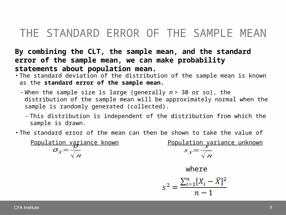
THE STANDARD ERROR OF THE SAMPLE MEAN

By combining the CLT, the sample mean, and the standard error of the sample mean, we can make probability statements about population mean.

• The standard deviation of the distribution of the sample mean is known as the standard error of the sample mean.

- When the sample size is large (generally n > 30 or so), the distribution of the sample mean will be approximately normal when the sample is randomly generated (collected).

- This distribution is independent of the distribution from which the sample is drawn.

• The standard error of the mean can then be shown to take the value of

Population variance known Population variance unknown

where

σ 𝑋=σ

√𝑛𝑠𝑋=

𝑠√𝑛

10

CENTRAL LIMIT THEOREM

Focus On: Importance

• With a large, random sample

- The distribution of the sample mean will be approximately normal.

- The mean of the distribution will be equal to the mean of the population from which the samples are drawn.

- The variance of the distribution will be equal to the variance of the population divided by the sample size when the population variance is known, and equal to the sample variance divided by the sample size when the population variance is unknown.

11

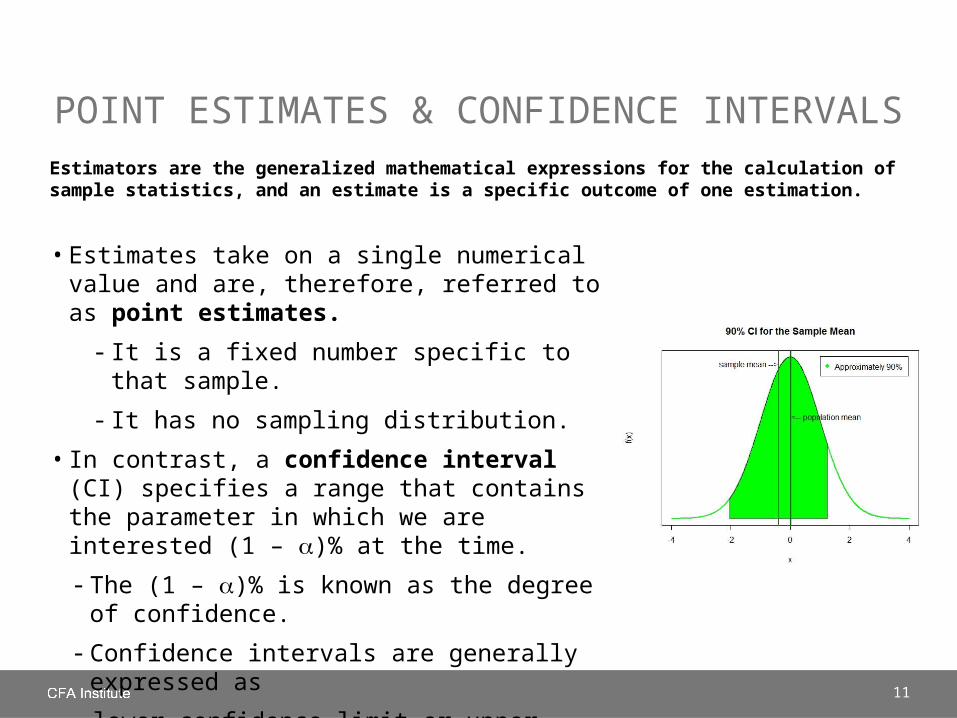
POINT ESTIMATES & CONFIDENCE INTERVALS

Estimators are the generalized mathematical expressions for the calculation of sample statistics, and an estimate is a specific outcome of one estimation.

• Estimates take on a single numerical value and are, therefore, referred to as point estimates.

- It is a fixed number specific to that sample.

- It has no sampling distribution.

• In contrast, a confidence interval (CI) specifies a range that contains the parameter in which we are interested (1 – a)% at the time.

- The (1 – a)% is known as the degree of confidence.

- Confidence intervals are generally expressed as

lower confidence limit or upper confidence limit.

12

ESTIMATOR PROPERTIES

There are a variety of estimators for each population parameter; accordingly, we prefer estimators that exhibit certain valuable properties.

1. Unbiasedness

- Occurs when the estimator expected value is equal to the value of the parameter being estimated.

- Examples: sample mean, sample standard deviation

2. Efficiency

- Occurs when no other estimator has a smaller variance.

- Examples: sample mean, sample standard deviation

3. Consistency

- Asymptotic in nature, thereby requiring a large number of observations.

- Occurs when the probability of obtaining estimates close to the value of the population parameter increases as sample size increases.

13

CONFIDENCE INTERVALS

Focus On: Constructing Confidence Intervals (CIs)

1. Point estimate = A point estimate of the parameter (a value of a sample statistic), such as the sample mean.

2. Reliability factor = A number based on the assumed distribution of the point estimate and the degree of confidence (1 − α) for the confidence interval.

3. Standard error = The standard error of the sample statistic providing the point estimate.

Normal pop, known s Unknown ,s large sample Unknown ,s small sample

Point estimate ± Reliability factor × Standard error

or𝑋 ±𝑧 α2

σ

√𝑛𝑋 ±𝑧 α

2

s

√𝑛𝑋 ±𝑡 α

2

s

√𝑛 𝑋 ±𝑡 α2

s

√𝑛

14

STUDENT’S t-DISTRIBUTIONWhen the population variance is unknown and the sample is random, the distribution that correctly describes the sample mean is known as the t-distribution.• The t-distribution has larger reliability (cutoff) values for a given level of alpha

than the normal distribution, but as the sample size increases, the cutoff values approach those of the normal distribution.

For small sample sizes, use of the t-distribution

instead of the z-distribution to determine

reliability factors is critical.

• The t-distribution is a symmetrical distribution

whose probability density function is defined

by a single parameter known as the

degrees of freedom (df).

15

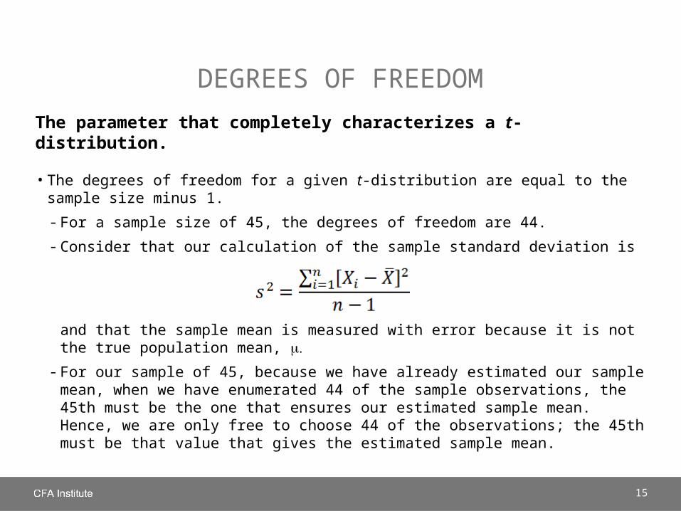
DEGREES OF FREEDOM

The parameter that completely characterizes a t-distribution.

• The degrees of freedom for a given t-distribution are equal to the sample size minus 1.

- For a sample size of 45, the degrees of freedom are 44.

- Consider that our calculation of the sample standard deviation is

and that the sample mean is measured with error because it is not the true population mean, . m

- For our sample of 45, because we have already estimated our sample mean, when we have enumerated 44 of the sample observations, the 45th must be the one that ensures our estimated sample mean. Hence, we are only free to choose 44 of the observations; the 45th must be that value that gives the estimated sample mean.

16

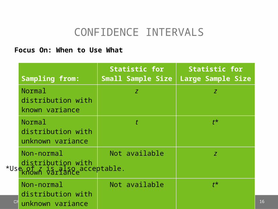
CONFIDENCE INTERVALS

Focus On: When to Use What

Sampling from: Statistic for Small

Sample Size Statistic for Large

Sample Size

Normal distribution with known variance

z z

Normal distribution with unknown variance

t t*

Non-normal distribution with known variance

Not available z

Non-normal distribution with unknown variance

Not available t*

*Use of z is also acceptable.

17

CONFIDENCE INTERVALS

Focus On: Calculations

You have a client with a target rate of return of 10% who would like to be 90% certain her realized return will include her target return. Construct a 90% confidence interval for each of the investments in the table, and determine whether each contains her target return.

Portfolio

Normal Population

Known Variance Unknown Variance,Small Sample

Unknown Variance,Large Sample

Target = 0.1 (1) (2) (3)

E(R) = .014 0.11 0.25

Std Dev = .020 0.08 0.27

n = 15 20 45

18

CONFIDENCE INTERVALS

Focus On: Calculations

For strategy (1), we use a z-statistic because the population variance (standard deviation) is known and the population is normally distributed.

Portfolio

Normal Population

Known Variance Unknown Variance,Small Sample

Unknown Variance,Large Sample

Target = 0.1 (1) (2) (3)

E(R) = .014 0.11 0.25

Std Dev = .020 0.08 0.27

n = 15 20 45

𝑋 ±𝑧 α2

σ

√𝑛=0.01±1.645

0.02

√15=[0.0055,0 .0225]

19

CONFIDENCE INTERVALS

Focus On: Calculations

For strategy (2), we use a t-statistic because the population variance (standard deviation) is unknown and the population is small and normally distributed.

Portfolio

Normal Population

Known Variance Unknown Variance,Small Sample

Unknown Variance,Large Sample

Target = 0.1 (1) (2) (3)

E(R) = .014 0.11 0.25

Std Dev = .020 0.08 0.27

n = 15 20 45

𝑋 ±𝑡 α2

𝑠√𝑛

=0.11±1.7290.08

√20=[0.0791,0 .1409]

20

CONFIDENCE INTERVALS

Focus On: Calculations

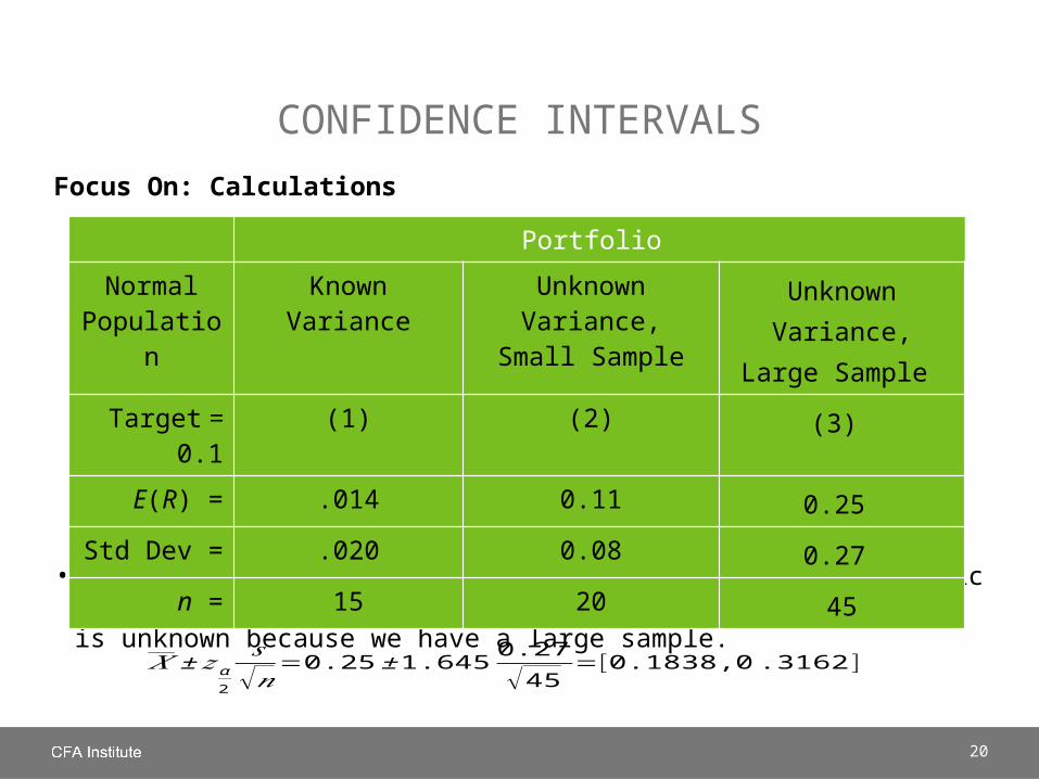
• For strategy (3), we can use a z-statistic or a t-statistic even though the population variance (standard deviation) is unknown because we have a large sample.

Portfolio

Normal Population

Known Variance Unknown Variance,Small Sample

Unknown Variance,Large Sample

Target = 0.1 (1) (2) (3)

E(R) = .014 0.11 0.25

Std Dev = .020 0.08 0.27

n = 15 20 45

𝑋 ±𝑧 α2

𝑠√𝑛

=0.25 ±1.6450.27

√45=[0.1838,0 .3162]

21

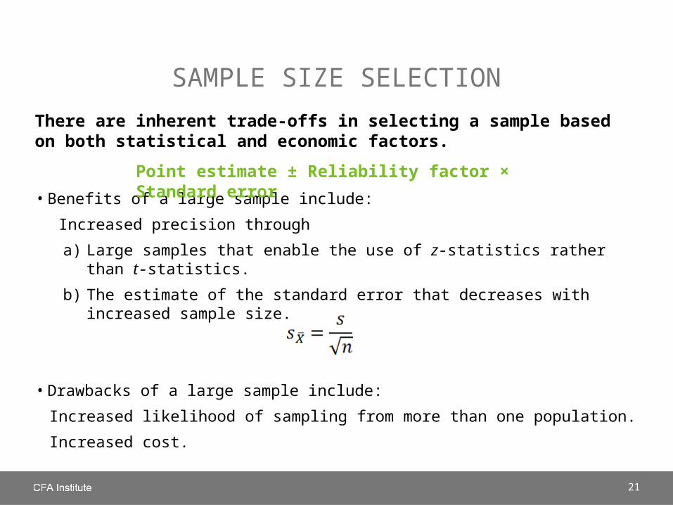
SAMPLE SIZE SELECTION

There are inherent trade-offs in selecting a sample based on both statistical and economic factors.

• Benefits of a large sample include:

Increased precision through

a) Large samples that enable the use of z-statistics rather than t-statistics.

b) The estimate of the standard error that decreases with increased sample size.

• Drawbacks of a large sample include:

Increased likelihood of sampling from more than one population.

Increased cost.

Point estimate ± Reliability factor × Standard error

22

DATA-MINING BIAS

“If you torture the data long enough, it will confess.” –reportedly said in a speech by Ronald Coase, Nobel laureate

• Data-mining bias results from the overuse and/or repeated use of the same data to repeatedly search for patterns in the data.

- If we were to test 1,000 different variables, 50 of them would be significant at the 5% level even though the significance is just an artifact of the testing error rate.

- This approach is sometimes called a “kitchen sink” problem.

- Economic and financial decisions made on the basis of these tests will be inherently flawed.

- There is no true underlying economic rationale for the relationship distinct from the testing phenomenon.

• To verify the relationship and/or discover data-mining biases, we can conduct out-of-sample tests.

No story No future

23

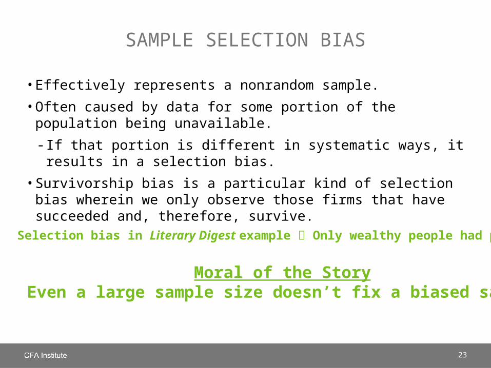
SAMPLE SELECTION BIAS

• Effectively represents a nonrandom sample.

• Often caused by data for some portion of the population being unavailable.

- If that portion is different in systematic ways, it results in a selection bias.

• Survivorship bias is a particular kind of selection bias wherein we only observe those firms that have succeeded and, therefore, survive.

Selection bias in Literary Digest example Only wealthy people had phones.

Moral of the Story Even a large sample size doesn’t fix a biased sample.

24

LOOK-AHEAD BIAS AND TIME-PERIOD BIAS

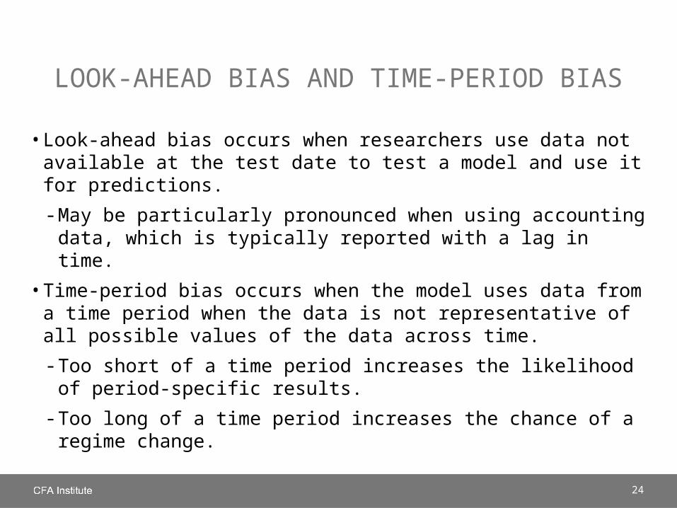
• Look-ahead bias occurs when researchers use data not available at the test date to test a model and use it for predictions.

- May be particularly pronounced when using accounting data, which is typically reported with a lag in time.

• Time-period bias occurs when the model uses data from a time period when the data is not representative of all possible values of the data across time.

- Too short of a time period increases the likelihood of period-specific results.

- Too long of a time period increases the chance of a regime change.

25

SUMMARY

• The quality of the sample is critically important when conducting or evaluating the results of a study.

• To draw valid inferences, the sample must be random in order to avoid a host of potential, often insidious, biases.

• When we have a random sample or samples, we can use the central limit theorem to conduct tests that compare the mean value of the sample with its value relative to a possible underlying population value.

- The appropriate test will differ as a function of our knowledge of the underlying population.

BOND INDEX AND STRATIFIED SAMPLING

Suppose you are the manager of a mutual fund indexed to the Lehman Brothers Government Index. You are exploring several approaches to indexing, including a stratified sampling approach. You first distinguish agency bonds from US Treasury bonds.

For each of these two groups, you define 10 maturity intervals: 1–2 years, 2–3 years, 3–4 years, 4–6 years, 6–8 years, 8–10 years, 10–12 years, 12–15 years, 15–20 years, and 20–30 years. You also separate the bonds with coupons (annual interest rates) of 6% or less from the bonds with coupons of greater than 6%.

BOND INDEX AND STRATIFIED SAMPLING

1. How many cells or strata does this sampling plan entail?2(10)(2) = 40

2. If you use this sampling plan, what is the minimum number of issues the indexed portfolio can have?

40, so that you have no empty cells

3. Suppose that in selecting among the securities that qualify for selection within each cell, you apply a criterion concerning the liquidity of the security’s market. Is the sample obtained random? Explain your answer. No. Now not every bond has an equal probability of being

accepted.