quantitative full-colour transmitted light microscopy and
TRANSCRIPT

HAL Id: hal-00662353https://hal.archives-ouvertes.fr/hal-00662353
Submitted on 27 Jul 2015
HAL is a multi-disciplinary open accessarchive for the deposit and dissemination of sci-entific research documents, whether they are pub-lished or not. The documents may come fromteaching and research institutions in France orabroad, or from public or private research centers.
L’archive ouverte pluridisciplinaire HAL, estdestinée au dépôt et à la diffusion de documentsscientifiques de niveau recherche, publiés ou non,émanant des établissements d’enseignement et derecherche français ou étrangers, des laboratoirespublics ou privés.
Quantitative full-colour transmitted light microscopyand dyes for concentration mapping and measurement of
diffusion coefficients in microfluidic architecturesMartinus H. V. Werts, Vincent Raimbault, Rozenn Texier-Picard, Rémi
Poizat, Olivier Français, Laurent Griscom, Julien R. G. Navarro
To cite this version:Martinus H. V. Werts, Vincent Raimbault, Rozenn Texier-Picard, Rémi Poizat, Olivier Français, etal.. Quantitative full-colour transmitted light microscopy and dyes for concentration mapping andmeasurement of diffusion coefficients in microfluidic architectures. Lab on a Chip, Royal Society ofChemistry, 2012, 12, pp.808-820. �10.1039/c2lc20889j�. �hal-00662353�

Quantitative full-colour transmitted light microscopy and dyes for concentration mapping and measurement of diffusion coefficients in microfluidic architectures
Martinus H. V. Werts,*a,b Vincent Raimbault,c Rozenn Texier-Picard,a,d Rémi Poizat, a,b
Olivier Français,b,e Laurent Griscom,a,b and Julien R. G. Navarroa,b
a Ecole Normale Supérieure de Cachan-Bretagne, UEB, Campus de Ker Lann, F-35170 Bruz, Franceb CNRS, SATIE (UMR8029), ENS Cachan-Bretagne, UEB, Campus de Ker Lann, F-35170 Bruz, Francec CNRS, IMS (UMR5218), Université de Bordeaux, 351 cours de la Libération, F-33405 Talence Cedex, Franced CNRS, IRMAR (UMR6625), ENS Cachan-Bretagne, UEB, Campus de Ker Lann, F-35170 Bruz, Francee Ecole Normale Supérieure de Cachan, 61 Avenue du Président Wilson, F-94235 Cachan Cedex, France
* corresponding author
Author manuscript for:
Lab on Chip 2012, 12, 808-820
DOI: 10.1039/C2LC20889J
Supplementary information
Electronic supplementary information (ESI) available. See DOI: 10.1039/c2lc20889j
published as: M. H. V. Werts et al., Lab on Chip 2012, 12, 808-820 1/33

Table of contents graphic
Abstract
A simple and versatile methodology has been developed for the simultaneous measurement
of multiple concentration profiles of colourants in transparent microfluidic systems, using
conventional transmitted light microscopy, a digital colour (RGB) camera and numerical
image processing combined with multicomponent analysis. Rigourous application of Beer-
Lambert law would require monochromatic probe conditions, but in spite of the broad
spectral bandwidths of the three colour channels of the camera, a linear relation between the
measured optical density and dye concentration is established under certain conditions. An
optimised collection of dye solutions for the quantitative optical microscopic characterisation
of microfluidic devices is proposed. Using the methodology for optical concentration
measurement we then implement and validate a simplified and robust method for the
microfluidic measurement of diffusion coefficients using an H-filter architecture. It consists
in measuring the ratio of the concentrations of the two output channels of the H-filter. It
enables facile determination of the diffusion coefficient, even for non-fluorescent molecules
and nanoparticles, and is compatible with non-optical detection of the analyte.
published as: M. H. V. Werts et al., Lab on Chip 2012, 12, 808-820 2/33

1 Introduction
Solutions of food dyes or biological stains are frequently used to visualise fluidic channels in
transparent microsystems using transmitted light microscopy. In most cases these dyes are
used for qualitative purposes, although they have been used for quantitative measurements,
such as in situ channel height1 and concentration profiles.2 Offline UV-visible absorbance
measurements have been used for microfluidic flow rate determination.3 Quantitative
measurements of concentration profiles4-7 in microfluidics are mostly achieved using
fluorescence imaging and fluorescent probes which requires sensitive detectors and suitable
microscope optics and hardware.
Previous work on absorbance imaging in transmitted light microscopy used narrow-band
light sources (either via monochromators or band pass filters) in combination with
monochrome cameras.1,2,8-13 Conventional transmitted light microscopes are readily equipped
with colour RGB (red-green-blue) cameras. One goal of this work is to establish to what
extent full-colour transmitted light imaging using RGB cameras can be combined with
suitable dye solutions to enable the simultaneous measurement of multi-component
concentration distributions. The spectral bands covered by each of the colour channels are
rather wide (> 100 nm), which is at odds with rigourous application of Beer-Lambert law that
requires monochromatic light.14 In the present work it is shown that within certain limits
Beer-Lambert law can still be applied to relate transmitted light (RGB) intensities to dye
concentrations.
The choice of dyes for use in microfluidics is vast, many are available in different
formulations. Optimised protocols describing recommended concentrations, solution
composition etc. for microfluidics are not readily available. This may lead to a number of less
desirable situations such as the use of unnecessarily high dye concentrations or the use of
inks of unknown proprietary composition. Here we study the properties of a small collection
of organic dyes and their application in quantitative studies of microfluidic architectures, in
order to establish a versatile collection of complementary dye solutions of known and well-
defined composition.
published as: M. H. V. Werts et al., Lab on Chip 2012, 12, 808-820 3/33

When calibrated, quantitative measurements using these dyes in transmitted light
microscopy are indeed possible. In this paper, conditions are established for the
measurement of multicomponent concentration profiles using conventional transmitted light
microscopes equipped with suitably adjusted RGB cameras. In view of the use of non-
monochromatic detection, it is necessary to verify linearity of the absorbance signal for each
dye. Moreover, the additivity of the absorbance signals for two dyes needs to be checked in
the case of multicomponent detection. The methodology presented can naturally be applied
to other dyes than those used in this paper, and we demonstrate the relevance of the method
for concentration mapping of 13 nm diameter gold nanoparticles diffusing in a microfluidic
circuit.
Building on transmitted-light based concentration measurements, we propose a microfluidic
method for the measurement of diffusion coefficients which is a modification of the T-
sensor/H-filter architectures15-19 often used for studying the molecular diffusion of
fluorescent objects. The alternative method presented here enables the measurement of
diffusion coefficients of nonfluorescent species using transmitted light microscopy, with the
further possibility to even use non-optical methods for detecting the diffusing species. The
method is applied to the (mostly non-fluorescent) food dyes studied as well as to (non-
fluorescent) gold nanoparticles.
Finally, we illustrate the use of quantitative full colour transmitted light microscopy in the
characterisation of typical microfluidic mixers and gradient generators. Not only do
optimised dye solutions and optimised image acquisition immediately generate visually
pleasing photographs, they also render these images amenable to multicomponent
concentration measurements that can reveal minor details in the functioning of microfluidic
devices not immediately recognisable in the initial images.
2 Dyes and solutions
2.1 Materials
As a solvent for the studies in this work we exclusively use phosphate-buffered saline
solution (PBS; 10 mM phosphate buffer at pH 7.4 with 137 mM NaCl and 2.7 mM KCl in
water) as this provides a constant physicochemical environment for all dyes, allowing
published as: M. H. V. Werts et al., Lab on Chip 2012, 12, 808-820 4/33

multiple dyes to be used simultaneously without a mismatch in either pH or ionic strength.
Pure water has an unstable pH under ambient conditions.20 Additionally, ionic strength is an
important physicochemical parameter. Most dyes used here are not sensitive to pH within
the pH range 5-9, and many will very likely give consistent results when used with pure
water, provided that they are used as their water-soluble salts. However, when possible a
saline buffer such as PBS is the preferred choice. PBS solutions were prepared from pre-
formulated powder in individual pouches (Sigma/Aldrich). It is noted that in the
microfluidic literature PBS (phosphate buffer containing also NaCl and KCl) is sometimes
unfortunately confused with simple phosphate buffer (without additional salts).
The dyes were obtained as pure powders and used as received. The dyes chosen are either
food dyes or stains for biological microscopy (or both). Some of the food dyes may be
obtained in solution from grocery stores as food coloring, but these preparations contain
several additives such as propylene glycol and preservatives, and are of unknown
concentration. We did not compare these preparations with the PBS solutions of the pure
dyes used in this work. Although – depending on the local legislation - most dyes are
considered to be safe when used as a food additive in a dilute form, the pure powders should
be handled with care, since these are the dye in high dose, and some are considered irritants,
and even poisons at high concentration.
The choice of dyes was inspired by a survey of microfluidic literature (see e.g. Refs. 21 and
22), chemical experience and commercial availability. One particular goal was to obtain a
combination of three dyes corresponding to colours complementary to red, green, and blue,
i.e. cyan, magenta and yellow, as this will enable the best colour separation between the three
dyes in a colour camera. Overlapping colour responses, however, is not necessarily a
problem, as analytical chemical multicomponent analysis methodology is capable of
transforming such overlapping responses into individual component concentrations.
The identification of suitable yellow (Tartrazine) and cyan (Fast Green) dyes was
straightforward, but finding the best water-soluble magenta dye proved more difficult, and
this explains the preponderance of red-magenta in the selection of dyes studied. Dyes were
chosen from the family of traditional food dyes (water-soluble azo dyes and related
compounds), but we also selected several xanthene dyes (fluorescein and derivatives).
published as: M. H. V. Werts et al., Lab on Chip 2012, 12, 808-820 5/33
Tartrazine (food additive E102, FD&C Yellow #5, CAS: 1934-21-0, mol. wt. 534.4 g mol -1) is a
yellow water-soluble negatively charged azo dye. Amaranth (food additive E123, FD&C Red
No. 2, CAS: 915-67-3, mol.wt. 604.5 g mol-1) is a red-magenta dye, also of the azo dye family.
In some countries it has been discontinued as a food dye, but is still commercially available
and useful as a microfluidic dye. Allura Red AC (food additive E129, FD&C Red #40, CAS:
25956-17-6, mol. wt. 496.4 g mol-1) is a red azo dye. It is sometimes used as a replacement
food dye for Amaranth (E123), with a hue that is red instead of magenta. Fast Green FCF
(food additive E143, FD&C Green #3, CAS: 2353-45-9, mol. wt. 808.9 g mol -1) is a water-
soluble triaryl dye which produces a cyan (blue-green) colour in PBS solution. In
combination with yellowish substances it produces a vivid green colour.
Fluorescein, free acid (no food dye designation, CAS: 2321-07-5, mol. wt. 332.3 g mol-1)
Fluorescein was also included in the study, since it can be used both in transmitted light as a
blue-absorbing yellow dye and in fluorescence measurements. It has been approved for
injection into the blood stream of humans, in particular for ocular angiography. Confusion
exists concerning the type of fluorescein to be used as a fluorescent tracer in fluidic channels.
Sometimes, fluorescein isothiocyanate (FITC) is used instead of fluorescein, with the implicit
incorrect assumption that these compounds are interchangeable. Fluorescein and FITC are
different compounds with different chemical and photophysical properties. In particular,
FITC readily hydrolyses in aqueous solution and is converted rapidly into aminofluorescein.
An aqueous solution of FITC is thus actually a solution of aminofluorescein, which has
different photophysical characteristics than fluorescein. For these reasons, it is preferable to
use fluorescein as a tracer rather than FITC. The use of the latter compound should be
reserved for its intended use, i.e. fluorescent labeling of (bio)macromolecules (with
subsequent purification of the labeled macromolecules).
Fluorescein – like most other xanthene dyes (such as Erythrosine and Rose Bengal) is sold in
various forms, in particular as the free acid or as its disodium salt. We used the free acid,
since there is a better guarantee of high purity. A disadvantage of the free acid is that its
dissolution in PBS, and even in aqeuous NaOH is slow. In order to be solubilised, the
(initially solid) free acid needs to be deprotonated, and this solid-liquid process is not fast.
Extensive sonication (1h) in PBS eventually leads to a limpid solution.
published as: M. H. V. Werts et al., Lab on Chip 2012, 12, 808-820 6/33
Erythrosin B, free acid (CAS: 15905-32-5, 834.9 g mol-1) is a red-magenta tetra-iodinated
derivative of fluorescein, and it is fluorescent (green-yellow), although its fluorescence
quantum yield is significantly lower than that of fluorescein. Its disodium salt is known as
food additive E127 or FD&C Red #3. Studies have shown that significant dye aggregation (>
10% of the dye molecules) occurs in water at concentration above 0.5 mM leading to altered
photophysical characteristics.23 Therefore, higher concentrations of the dye were avoided.
Rose Bengal (no food dye designation, CAS: 632-69-9, 1018 g mol-1) is also a magenta
derivative of fluorescein and is used as a biological stain in microscopy, as a photoinitiator for
photopolymerisation24 and as a photosensitiser for the generation of singlet oxygen (of
interest both in synthetic chemistry and in photodynamic therapy).25 At concentration above
0.5 mM, significant aggregation of the dye occurs.23
As a complement to organic dyes we studied solutions of 13 nm diameter gold nanoparticles
capped26 with thiooctic acid (AuTA). Gold and silver nanoparticles have an extremely strong
optical response related to the localised plasmonic resonance of their conduction electrons.27
This optical response manifests itself as visible light absorption, leading to burgundy red
coloration of gold nanoparticles, and – for particles of sufficient diameter – efficient resonant
light scattering.28,29 In combination with the possibility to functionalise these metal particles
with (bio)molecular functions30,31 the strong optical response makes gold and silver particles
interesting biophotonic transducers for sensitive detection in microfluidic volumes. The
solutions of AuTA nanoparticles used here are easily prepared, are stable against aggregation
(at basic pH) and can readily be concentrated to the concentrations necessary for observation
in microfluidic channels using transmitted light optical microscopy. The particles, however,
are not soluble in PBS solution, and therefore 1 mM aqueous NaOH was used as a solvent
instead.
2.2 Absorption spectra and extinction coefficients
Figure 1 displays the UV-visible absorption spectra of PBS solutions of the dyes. These
spectra illustrate their spectral complementarity, particularly of Tartrazine, Amaranth (or
Rose Bengal) and Fast Green. The wavelengths of the absorption maxima and the
corresponding extinction coefficients are listed in Table 1. These parameters are of use for
offline analysis of dye solutions. The magnitude of the extinction coefficients reveals the three
published as: M. H. V. Werts et al., Lab on Chip 2012, 12, 808-820 7/33

distinct chemical families of the dyes: azo dyes (εmax ~ 2 x 10⁴ M-1 cm-1), xanthene dyes (εmax ~
8 x 10⁴ M-1 cm-1) and Fast Green triarylmethane dye (εmax > 105 M-1 cm-1). For AuTA we list the
typical literature value for 13 nm diameter gold nanoparticles, which should be taken to be
accurate within ±20%.32 The high extinction coefficient for these particles makes that even the
concentrated solutions used for the microfluidic experiments reported here have a particle
concentration over a thousand times smaller than the dye solutions.
Figure 1. Normalised UV-visible absorption spectra of solutions of dyes in PBS solution. FL =Fluorescein, AR = Allura Red AC, EB = erythrosine B, TZ = tartrazine, AM = Amaranth, RB =Rose Bengal, FG = Fast Green FCF.
Table 1 also list the maximum recommended concentrations and the recommended
concentration of the dyes in PBS for use with a 100 µm high fluidic channel. The maximum
concentration was either limited to the solubility of the dye or to 4 mM. No concentrations
higher than 4 mM were tested, in view of the PBS solution being only 10 mM in buffering
phosphate. For the azo dyes the 4 mM concentration does not seem to be a limit, but using
these concentrations would need a change of buffer (e.g. 0.1 M phosphate buffer at pH 7.4)
and additional validation. Except for Fast Green, which has some headroom, the
concentrations for use with 100 µm are limited by the maximum recommended
concentration. For use with thicker channels, the solutions should be diluted proportionally.
published as: M. H. V. Werts et al., Lab on Chip 2012, 12, 808-820 8/33

Thinner channels can be studied with the same concentrations as for 100 µm channels, with
an obvious loss in optical density. On basis of dilution experiments we anticipate that
channels as thin as 20 µm should still work well for quantitative transmitted light
microscopy. The concentration of Fast Green may still be increased for such studies.
Table 1. UV-vis data, solubility in PBS, maximum recommended concentration, and recommendeddye concentration for studying a 100 µm high channel. Recommendation takes into accountsolubility and acceptable optical densities
εmax / L mol-1
cm-1 λmax / nm Cmax
/ mMC100µ
/ mM
Tartrazine(a) 2.5(±0.2) x 104 427.8(±0.6) 4(c) 4
Fluorescein(b) 7.4(±0.6) x 104 490.5(±0.4) 0.4(d) 0.4
Allura Red AC(a) 2.4(±0.1) x 104 497.5(±0.4) 4(c) 4
Amaranth(a) 2.3(±0.2) x 104 521.0(±0.5) 4(c) 4
Erythrosin B (b) 9.8(±0.2) x 104 526.3(±0.1) 0.5(e) 0.5
Rose Bengal(b) 9.5(±0.5) x 104 549.4(±0.2) 0.5(e) 0.5
Fast Green FCF(a) 1.2(±0.1) x 105 623.2(±0.1) 4(c) 1
AuNP-TA, 13 nm(f) 2.4 x 10⁸ (g) 525.5 n.a. 0.3 µM(a) solution prepared from the sodium salt as received (see text)(b) solution prepared from dye in its free acid form as received (see text) (c) no higher concentrations were investigated (see text)(d) solubility limited(e) aggregation phenomena may lead to nonlinearities > 0.5 mM23
(f) solvent: 1 mM NaOH(aq)(g) literature value32
2.3 Practical considerations
All solutions (i.e. the dyes in PBS at millimolar concentrations) were stored in the dark at 4°C
in glass vials or Nalgene flasks. Under these conditions, the dyes solutions are usable in
transmitted light micrscopy for several months. Comparison of the UV-visible spectra of aged
solutions with freshly prepared solutions showed no significant degradation of the solutions
after 3 months for tartrazine, amaranth, allura red or fast green. The latter two were verified
to be stable even after 9 months. The spectra of the solutions of the xanthene dyes
(Fluorescein, Erythrosin B, Rose Bengal) showed small signs of degradation after 3 months.
The degradation manifests itself in UV-visible spectroscopy as a minute but detectable blue
shift of the absorption maxima (~ 0.5 nm), and a slight decrease of the maximum absorbance
published as: M. H. V. Werts et al., Lab on Chip 2012, 12, 808-820 9/33
(< 5%). This small degradation does not significantly affect the measurements in microfluidic
channels, but nevertheless indicates that fresh solutions should be prepared after 3 months.
In contrast to the frequently used fluorescent dye Rhodamine B,33 none of the dyes reported
here stains PDMS, which means that many experiments involving different dye solutions can
be performed on the same PDMS device, without degradation due to irreversible staining of
the PDMS channel walls. Rinsing the devices with PBS or pure water rapidly restores the
PDMS device to their initial uncoloured state.
3 Quantitative measurements of dyes in transmitted light microscopy using full-colour imaging
3.1 Measurements of optical densities using a colour camera in transmitted light microscopy
The transmittance of light can be converted into absorbance, and subsequently into
concentration values using the well-known Beer-Lambert law. One of the conditions for the
Beer-Lambert law to hold is that the light used be monochromatic (or at least that neither the
extinction coefficient of the substance nor the probe light intensity vary over the wavelength
interval used). Using non-ideal conditions, i.e. using spectroscopic bandwidths that are large
compared to the width of the spectral features, leads to the introduction of stray light terms
into the Beer-Lambert formula, and to a loss of linearity of the absorbance signal.14
Most digital colour cameras divide the visible spectrum into three wide wavelength ranges
using Bayer filters, which consist of 2 x 2 pixel blocks containing 2 green pixels and 1 red and
1 blue pixel.34 Each pixel block gives rise to one colour pixel containing three intensity values
for the red, green and blue (RGB) channels. The spectral responses for the red, green and
blue channels are similar among CCD cameras. In view of the very large spectral bands used
in the Bayer filter for each colour channel, the pixel-wise application of the Beer-Lambert law
to digital colour images is expected to suffer from deviations from the ideal linear behaviour.
This limitation will depend in particular on the degree of spectral overlap of the dye used
with the spectra of the light source (often a tungsten-halogen lamp) and the spectral response
of the Bayer filter for the colour channel. Each particular combination of light source,
microscope and colour camera will to some extent show a different spectral response, and
therefore it is necessary to calibrate the specific response for a dye solution for a given
published as: M. H. V. Werts et al., Lab on Chip 2012, 12, 808-820 10/33

microscope, and to determine the concentration range in which the response is linear. Here
we will demonstrate the method for one particular microscope set-up. We will also compare
the results for that set-up with a different microscope set-up, showing that the small
difference in colour responsitivities necessitate calibration and linearity checks for each dye-
microscope combination.
The microfluidic studies of the dye solutions were carried out on a specifically designed
microfluidic platform (Figure 2), dubbed 'Péclet-O-Matic', which is used alternatively as a
simple flow cell, a T-sensor, an H-filter or a passive mixer. The passive mixer may include an
additional staggered herringbone35 motif (see Figure SI-6). The channels were fabricated by
moulding PDMS against a photolithographically defined SU8 mould. The resulting PDMS
slab was bound to microscope slides or cover slips using plasma bonding (see Experimental
Section). The focal plane for observation was chosen so as to be half-way the channel height.
This results in the channel borders (and other out-of-focus contributions) being slightly
blurred, and steep edges in the image profile being smoothed.
Figure 2. Microfluidic architecture of the 'Péclet-O-Matic'. The straight arrows indicate flowdirection. "A" and "B" indicate the two input channels that join at "1", and are split again at "2".Optical measurement of dye concentration in each channel takes place at "3".
The device contains two 100 µm wide and 100 µm high input channels ("A" and "B", Figure 2)
that meet at a T junction ("1"). Then follows a 54 mm long, 200 µm wide interaction zone,
after which the flows are split (point "2", Figure 2). Extra channel length (100 mm each) is
then added to homogenize the concentration profile before optical detection at point "3"
published as: M. H. V. Werts et al., Lab on Chip 2012, 12, 808-820 11/33

(Figure 2). Concentration of dye at any point in the microfluidic channel may be obtained
from transmitted light microscopy through Beer-Lambert law.
Application of Beer-Lambert law requires measurement of incident (I0) and transmitted (I)
light intensities. I0 and I can be taken from two separate images (a reference image and the
image of the microfluidic channels with dye solutions), but I0 values may also be obtained by
interpolating a baseline between two transparent regions on the image. The advantage of the
latter method is that it is insensitive to changes in lighting conditions and electric gain
settings between images. The former method is similar to a flat-field correction in which the
image is corrected for inhomogeneous illumination and imaging conditions.
It is essential to optimise light intensity and image acquisition parameters. We found it
beneficial to include colour ("daylight") correction filters in the microscope illumination path.
Many microscopes have this installed as an option. A BG34 glass filter may be used as well.
The effect of this filter is to diminish the red light intensity, thus enhancing the contribution
of the blue (and green) channels. The light source should always be operated at the same
current setting, since the lamp emission spectrum depends on the temperature of the
filament. If necessary, grey neutral density filters can be used to attenuate the light, in order
to avoid changing the lamp current. Before beginning actual measurements the light source
was left to stabilise at a given current setting (30 minutes, typically). Histograms of the
intensity values for each colour channel in the images recorded can be used for checking
stable operation.
The camera should be set to output a signal linearly proportional to the light intensity. Any
"gamma" correction should be switched off. Importantly, any automatic white balance and
background correction, as well as automatic gain adjustments should be switched off as well.
The electronic gain for each colour channel needs to be adjusted manually, and should be
kept minimal in order to reduce noise. The gain settings can be adjusted to equilibrate the
levels of each colour channel (which corresponds to performing a manual white balance).
Most scientific and industrial imaging cameras allow for precise parametrization either via
the acquisition software of directly on the camera.
published as: M. H. V. Werts et al., Lab on Chip 2012, 12, 808-820 12/33

Any dark offset should be set such that in the absence of light on the camera the electric
signal (pixel value) is low, but never zero. This is necessary for avoiding the truncation of
low-level noise values that would occasionally drop below zero and for which the analog-to-
digital conversion will simply return zero. A proper dark-corrected image in the absence of
light should have noise fluctuating around zero.
For optimising lighting and imaging settings we found it useful to record images of
transparent zones of the microfluidic devices and analyse the intensity histograms for each
image colour channel. Light intensity and manual gain and dark offset are then regulated
such that dark images produce an intensity of 5% of the maximum value (~15 in 8-bit colour
values) and transparent, uncoloured zones produce an intensity of 80% of the maximum
value (~200 in 8-bit values). Signal-to-noise can be significantly improved by averaging† over
several images, taken from the same zone using identical illumination and gain settings.
With the image acquisition having been optimised, we can now record images and the
process them to obtain three-colour absorbance profiles. For the description of the image
processing that follows, each colour channel of the image is considered separately, giving a
(monochromatic) matrix M(R), M(G) or M(B)) for each colour channel. These image matrices are
conditioned such that they contain only the part of the image that will contribute to the
generation of the absorbance profile. Additionally, the image is oriented such that fluid
propagation is oriented along the matrix columns and the absorption profile to be extracted
is in the matrix row direction (See the top of Figure 3). The dimensions of M(R,G or B) are Nlines x
Npoints, where Nlines is the number of image lines to be summed and Npoints are the number of
points in the profile to be extracted.
Both a raw image Mraw(R,G,B) and a dark image Mdark
(R,G,B) are recorded. The dark image is
obtained by blocking the light source, and will be used to correct for the camera dark current.
The dark corrected image matrix M is then obtained (Equation 1).
M(R,G,B)=Mraw
(R,G,B)−Mdark
(R,G,B) (Equation 1)
†This averaging should be done using high bit depth (16-bit, 32-bit) or even floating point digital images
published as: M. H. V. Werts et al., Lab on Chip 2012, 12, 808-820 13/33

Additionally it may be possible to record a flat-field image Mbright(R,G,B) by recording a
completely white (and structureless) zone of the device, and use this image to correct
(Equation 2) for variations in the illumination and imaging efficiency ('vignetting').
M(R,G,B)=
Mraw(R,G,B)
−Mdark(R,G,B)
Mwhite(R,G,B)
−Mdark(R,G,B) (Equation 2)
From the image M(R,G,B) we can extract an intensity profile by creating a row vector whose
components are obtained by summing over each of the colums (Equation 3). The matrix 11 x
Nlines is a row matrix of which all of the Nlines elements are 1 (a 1 x Nlines 'ones' matrix). The
middle part of Figure 3 shows an example of one of the three colour profiles obtained from
the image in the top.
I(R,G,B)=11 x N lines
M(R,G,B) (Equation 3)
A baseline profile I0(R,G,B) is obtained via interpolation by defining the PDMS areas outside the
fluidic channels as zones on which the baseline is modeled (e.g. by a linear or a parabolic
function). The middle part of Figure 3 shows an interpolated baseline of the sort. In the case
of an image that has been flat-field corrected (Equation 2), the baseline will be a constant
(ideally equal to 1), and interpolation will not be necessary. However, obtaining I0 directly
from the image by interpolation is a convenient and robust method and may in many cases
be more efficient than separate flat-field corrections. The absorption (or optical density)
profiles for each colour channel are obtained by application of Equation 4.
AR,G,B=−
10 logIprofR,G,B
I0R,G,B (Equation 4)
Row vectors A(R, G or B) then contain the absorbance (optical density) profiles and have
dimensions (1 x Npts). An example of the final set of colour optical density profiles is at the
bottom part of Figure 3. Near the microchannel edges the image and the ensuing optical
density profile is slightly distorted, due to refraction at the liquid-PDMS interface. This stems
from a refractive index mismatch between the aqueous solution chosen and the PDMS. The
affected regions were not included in any further analysis. If necessary, the solvent
composition may be changed such that its refractive index matches that of the microsystem
published as: M. H. V. Werts et al., Lab on Chip 2012, 12, 808-820 14/33

material.1 For PDMS, n ~ 1.43, this may be achieved using water-glycerol mixtures. This
should then be combined with a new calibration of the concentration measurement (see
Section 3.2 below).
Figure 3. Quantitative transmitted light microscopy of a channel containing interdiffusing laminarflows of Fast Green and Tartrazine in PBS. Top: colour transmitted-light micrograph (10x, NA 0.22objective) taken in a fluidic channel (just before point "2", Figure 2), and positioned such that theprofile to be extracted runs horizontally (along the matrix row direction). The image has the darksignal already subtracted. Middle: intensity profile (I) for the blue channel (solid line) obtained bysumming all column elements, baseline (I0) (dotted line) obtained through linear interpolation.Bottom: optical density (absorbance) profiles for each of the colour channels.
The set of three row vectors containing the colour intensity profiles can be combined into a 3
x Npts matrix containing the optical densities with each row containing an intensity profile
corresponding to a particular colour. The number of colours – or wavelength bands – may be
extended when more wavelength channels are used, such as in multispectral imaging. 9 The
three-colour absorbance profile matrix (which we will refer to as A) can be subjected to
analytical chemical multicomponent analysis, provided that the individual absorbance
published as: M. H. V. Werts et al., Lab on Chip 2012, 12, 808-820 15/33

responses are linearly proportional to the concentration (mathematically 'homogeneous') and
additive. These two conditions will be verified experimentally in the two next sections.
3.2 Linearity: Effective molar absorption coefficients (EMACs)
The Beer-Lambert law can be cast in the matrix form of Equation 5.
A=lEC (Equation 5)
Matrix A contains the absorbance (optical density) profiles and has dimensions (Nchannels x
Npts, with Nchannels = 3 for RGB imaging). The optical pathlength is denoted l, and is taken to be
equal to the channel height. The actual channel height of each device mould was measured
using a stylus profilometer (102...110 µm). Strictly speaking, the assumption that l equals the
channel height is only valid for light that traverses the channel perpendicularly. However, a
microscope objective collects light over a range of angles, defined by a cone with an aperture
2arcsin(NA), with NA being the numerical aperture of the objective. This leads to effective
optical pathlengths larger than the channel height, and may introduce a systematic error for
objectives with large NAs. Broadwell et al. found1 that for objectives of 10x or less these errors
are negligble (2.3% for 10x, NA 0.3). Therefore, the approximation that optical pathlength l
equals the channel height is valid, for the low NA objectives used in this work (NA 0.06 ...
NA 0.30), but higher NA objectives should be avoided, or properly corrected for.
The matrix C is an (Ncomp x Npoints) matrix which will contain the concentration profiles of each
of the components, with Ncomp being the number of components and Npoints the number of
data points representing the concentration profile. In normal UV-visible or IR absorption
spectroscopy, matrix E would contain the molar absorption coefficients (Nchannels x Ncomp). Since
we are dealing with broad-band, non-monochromatic probe light we prefer to refer to the
elements of E as effective molar absorption coefficients (EMAC).
In this section, we are interested in verifying experimentally a linear relationship between the
concentration and the optical density for individual dyes (Ncomp = 1). For our RGB images the
matrix E is therefore constructed as in Equation 6.
E=EMACREDEMACGREENEMACBLUE
(Equation 6)
published as: M. H. V. Werts et al., Lab on Chip 2012, 12, 808-820 16/33

Dilution series were made for each of the dyes investigated by using a staggered herringbone
mixer integrated in the interaction zone (between points "1" and "2", Figure 2; see Figure SI-6
for a micrograph), supplying one input with a concentrated solution of dye in PBS, the other
with only PBS. The volume fraction of the dye solution is then varied between 0% and 100%,
while keeping the total flow rate constant. The optical density of the solution is measured at
the output of the mixer (just before point "2", Figure 2). The concentration accross the
microfluidic output channel will be constant, and we take the average optical density
accross the channel (reducing Npoints to 1).
Interestingly, linear behaviour was observed for all dyes in the concentration range tested
(typical dilution curves are shown in Figure SI-1, Supporting Info). This is a non trivial
experimental result since we are working with non monochromatic detection, under
conditions where stray light may be significant. This said, the optical densities used never
exceed 1 meaning that at the most, 90% of the incident light is absorbed, which likely
contributes to obtaining linear absorbance-concentration relationships. For both qualitative
and quantitative imaging it is beneficial to remain in the concentration range where the
solutions absorb at most 90 ... 95% of the light (OD 1 ... 1.3 ) in any of the colour channels. If
saturated colours are sought after (in qualitative imaging) there is no need to aim beyond OD
2, meaning that dye solution concentrations remain in the millimolar range for 100 µm
channel height.
Table 2 compiles the EMACs determined for the dyes on a particular light source –
microscope – colour camera combination (see Experimental Section). Surprisingly, certain
EMACs are slightly negative (a negative slope of the optical density-concentration plot). This
may be attributed to an electronic artefact (negative cross-talk), and/or fluorescence
emission. Even for quantitative measurements this is not a problem: the negative EMAC
value for a dye should indeed be included as such in the application of Equation 5.
published as: M. H. V. Werts et al., Lab on Chip 2012, 12, 808-820 17/33

Table 2. Effective molar absorption coefficients for each colour channel for the principal light source– microscope – camera combination used in this work.
EMACRED
/ mM-1mm-1EMACGREEN
/ mM-1mm-1EMACBLUE
/ mM-1mm-1
Tartrazine -0.02 ± 0.01 0.12 ± 0.01 1.4 ± 0.1
Fluorescein -0.31 ± 0.13 1.2 ± 0.1 4.2 ± 0.2
Allura Red -0.13 ± 0.01 1.0 ± 0.1 1.3 ± 0.1
Amaranth 0.05 ± 0.03 1.9 ± 0.2 0.9 ± 0.1
Erythrosine B -0.75 ± 0.08 3.8 ± 0.2 1.5 ± 0.1
Rose Bengal 0.01 ± 0.09 4.5 ± 0.2 -0.16 ± 0.03
Fast Green 7.0 ± 0.4 0.52 ± 0.05 0.29 ± 0.02
AuNP-TA(a,b) (3.9 ± 0.8) x 103 (14 ± 3) x 103 (10 ± 2) x 103
(a) 1 mM NaOH (aq), instead of PBS(b) uncertainty on actual NP concentration dominates the interval on EMAC values
Since EMACs depend on the spectral overlap between the probe light spectrum, the spectral
response of all optics and camera colour channels and the dye, they will depend on the
equipment used, and need to be characterised for each particular set-up. Differences are not
expected to be enormous, since the spectral response of Bayer filters and silicon-based
detectors do not change much between cameras. We tested this by using a second alternative
set-up (see Experimental Section). Indeed, the EMACs of a selection of dyes follow the same
trend as in Table 2, although their absolute values can deviate by more than 50% between
microscopes (see Supporting Info). We noted that the separation between colour channels
was less efficient in the lower cost CMOS camera compared to the CCD camera. In particular
the blue channel was less efficient, and in this channel linearity was lost for tartrazine at > 2
mM.
The instrument-dependence of EMACs contrast with the instrument-independence of
conventional molar absorption coefficients determined under near-ideal spectroscopic
conditions. Such near-ideal conditions may be created in an optical microscope by using
narrow optical band-pass filters, an approach successfully employed for quantifying channel
heights and indicator concentrations in microfluidics.1,2 The aim of the present work is to
establish to what extent unmodified RGB cameras may be used for quantitative concentration
measurements, so that colour micrographs can be taken that are visually pleasing and at the
published as: M. H. V. Werts et al., Lab on Chip 2012, 12, 808-820 18/33
same time contain useful quantitative data. Moreover, the simultaneous recording of three
colour channels provides in principle simultaneous access to the concentrations of three
components.
3.3 Additivity of colour responses
In order to obtain concentrations from optical densities for dyes with previously measured
EMACs, Equation 5 can be inverted (Equation 7).
C=1lE−1 A (Equation 7)
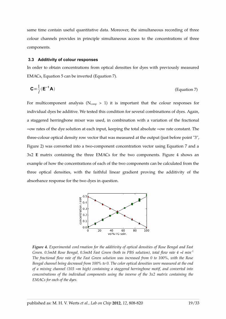
For multicomponent analysis (Ncomp > 1) it is important that the colour responses for
individual dyes be additive. We tested this condition for several combinations of dyes. Again,
a staggered herringbone mixer was used, in combination with a variation of the fractional
flow rates of the dye solution at each input, keeping the total absolute flow rate constant. The
three-colour optical density row vector that was measured at the output (just before point "3",
Figure 2) was converted into a two-component concentration vector using Equation 7 and a
3x2 E matrix containing the three EMACs for the two components. Figure 4 shows an
example of how the concentrations of each of the two components can be calculated from the
three optical densities, with the faithful linear gradient proving the additivity of the
absorbance response for the two dyes in question.
Figure 4. Experimental confirmation for the additivity of optical densities of Rose Bengal and FastGreen. 0.5mM Rose Bengal, 0.5mM Fast Green (both in PBS solution), total flow rate 4 µl min-1.
The fractional flow rate of the Fast Green solution was increased from 0 to 100%, with the RoseBengal channel being decreased from 100% to 0. The color optical densities were measured at the endof a mixing channel (103 µm high) containing a staggered herringbone motif, and converted intoconcentrations of the individual components using the inverse of the 3x2 matrix containing theEMACs for each of the dyes.
published as: M. H. V. Werts et al., Lab on Chip 2012, 12, 808-820 19/33

The simultaneous optical measurement of the concentration of each of the two dyes (Fast
Green and Rose Bengal) reproduces the concentration gradient generated by varying the
relative flow rates of each of the dye solutions. This confirms the additivity of the optical
responses of the two dyes. Thus, it is possible to use food dyes for quantitative
multicomponent measurements in transmitted light microscopy. The approach can naturally
be extended to other dyes, in particular to indicators which exist as a mixture of two species
whose relative contribution depends on the concentration of an analyte. Also solutions of
gold (and silver) nanoparticles in combination with small dye molecules may be analysed. In
addition to a separation according to colour response (EMACs), such samples may also be
separated according to diffusion coefficients.
4 Ratiometric determination of diffusion coefficients using an H-filter architecture
Using the dye concentration measurement in transmitted-light microscopy on microfluidic
systems, we implement and validate a simplification of diffusion measurements using an H-
filter, that is based on the (optical) measurement of the ratio of the concentrations in the
channels at the output of the H-filter (point "3", Figure 2).
Near the interface between two (infinitely wide) laminar flows, one of which initially
contains all the analyte at concentration C0, the other only solvent, the temporal evolution of
the analyte concentration profile is usually calculated using Equation 8.36,37
C x , t =12C 01−erf x
2Dt with erf z =2
∫0
z
exp −v2dv (Equation 8)
In Equation 8, x represents the position across the channel, with x=0 being the position of the
flow interface. Constant flow converts time t into a spatial coordinate along the channel. In
the microfluidic T-sensor15-18 architecture, diffusion coefficients are extracted by fitting
Equation 8 to steady-state fluorescence microscopy images of the T-junction.5,36 This
procedure is limited to fluorescent entities, or to entities that can be detected using
fluorescent probes (such as38 H+ and39 Ca2+).
We propose a modified microfluidic measurement of diffusion coefficients based on the
measurement of the concentration ratio between two laminar flows at the output of a H-filter.
published as: M. H. V. Werts et al., Lab on Chip 2012, 12, 808-820 20/33
The two laminar flows, one initially empty and one containing the substance under analysis,
meet at a T-junction are allowed to interact in a long channel, after which they are separated.
Subsequently, the analyte concentration ratio of the two outputs is measured. In the present
work, the concentration measurement will be done using transmitted light microscopy, using
the methodology described above, but may be replaced by other means of concentration
measurement (electrochemistry for example). Compared to fluorescence imaging, this
method greatly increases the range of species whose diffusion coefficient can be determined,
for example to the nonfluorescent food dyes that we aim to characterise in view of their
application in quantitative microfluidic analysis.
Equation 8 is for the evolution of a front between two infinitely broad flows, one of which
initially contains all the analyte, the other only solvent. Defining the H filter as a microfluidic
channel (of limited width w, height h, length L) where two laminar flows (A and B) interact,
an analytic expression for the temporal evolution of the concentration profile across a
channel of limited width can be obtained using a Fourier approach. Such an approach has
for example been used in the systematic design of gradient generators,40 and has indeed been
suggested for describing diffusion in microchannels.41 In the case of the H filter architecture
used here we find
C x , t =C02
∑k=0
∞
−1k2C0
2k1exp −D
22k12
w2t cos 2k1
wx (Equation 9)
At the input of the H-filter flow A contains a solution of the analyte (dye) at a concentration
C0. Flow B contains only the solvent (buffer). At the output of the H-filter both flows are
separated (e.g. point "3" in Figure 2). The concentrations of the analyte in each of the
separated flows at the output are denoted CA and CB for flows A and B, respectively
(Equation 10).
CA=2w∫0
w /2
C x , t dx and CB=2w∫w /2
w
C x , t dx (Equation 10)
For the determination of diffusion coefficients using the ratiometric H filter method, a natural
way of expressing the experimental data may be plotting the ratio of CB and CA (equal to the
ratio of the absorbances, see below) as a function of flow rate. Using Equations 2 and 3, this
ratio can be expressed as Equation 11.
published as: M. H. V. Werts et al., Lab on Chip 2012, 12, 808-820 21/33

CBC A
=1−1
(Equation 11)
with
=∑i=0
∞
ci exp −k i t (Equation 12)
and c i=8
22i12
and k i=D
22i12
w2
The ξ function describes the extent of mixing (i.e. equal distribution of the analyte between
flows A and B), and is related to the observed concentration ratio according to Equation 13.
=CA−CBC ACB
(Equation 13)
These expressions describe the evolution of the (one-dimensional) concentration ratio in
time. Adding steady flow in a second dimension enables us to express t (which can be
assimilated to the average residence time of a molecule in the interaction zone) in terms of
the channel dimensions (h, w, and L) and the flow velocity U0 or the flow rate Vflow.
U 0=V flowhw
and t=LU 0
(Equation 14)
The series in Equation 9 and 12 converge quite quickly for large t (slow flow rates), and one
or two terms are generally sufficient to describe the concentration ratio as a function of flow
rate (see Supporting Info, Figure SI-2, for the convergence behaviour of Equation 12). When
applying Equation 14 to Equation 12, the Péclet number (Pe = U0w/D) appears naturally.
For solutions containing only a single detectable component we can express the
concentration ratio of analyte in flows A and B as the ratio of the measured absorbances
(ODA and ODB), applying Beer-Lambert law. In practice, these absorbance values are
obtained by averaging the values in each channel extracted from absorbance profiles
obtained at point "3" (Figure 2) using the method described in Section 3.1. The concentration
ratios then become optical density ratios, as per Equation 15.
CBC A
=ODB
ODAand
CA−CBC ACB
=ODA−ODB
ODAODB
= (Equation 15)
published as: M. H. V. Werts et al., Lab on Chip 2012, 12, 808-820 22/33

At sufficiently slow flow rates we can use only the first term of the series in Equation 12 and
linearize Equation 13. This gives Equation 16.
lnODA−ODBODAODB
=−Dln82 (Equation 16)
with =2 L
U 0w2=
2L h
V floww.
In Equation 16 the only experimentally unknown parameter is the diffusion coefficient D
which is the slope of the line obtained by tracing ln(ξ) as a function of τ. It is interesting to
note that ODA and ODB may be replaced by any other (processed) signal that is linearly
proportional to the concentration of the analyte, such as values from amperometry or
conductivity. All expressions are in SI units. A total flow rate of 1 µl min -1 amounts to Vflow =
1.667 x 10⁻¹¹ m3 s-1, for a 200 µm wide, 100 µm high channel.
Figure 5 exemplifies the experimental validity of the method for Allura Red in PBS, and 13
nm diameter AuTA particles in 1 mM aqueous NaOH. The optical densities were taken both
from the green and the blue camera channels. The ratios of the optical densities (i.e. the
concentrations) of the two H-filter outputs indeed follow the theoretical curve corresponding
to diffusion coefficient D = 3.4 x 10⁻¹⁰ m2 s-1 and D = 0.37 x 10⁻¹⁰ m2 s-1 for Allura Red and AuTA
particles, respectively. These correspond to a Stokes-Einstein hydrodynamic radius of 0.7 nm
for Allura Red and 6.5 nm for AuTA, in good agreement with the expected radii of the
objects.
published as: M. H. V. Werts et al., Lab on Chip 2012, 12, 808-820 23/33

Figure 5. Ratiometric determinations of the diffusion coefficient of Allura Red AC in PBS (squares)and 13 nm diameter AuTA nanoparticles (circles). The channel width is 200 µm, height 103 µm,interaction length 54 mm. Top: Ratio of the measured absorbances of channel B and A as a functionof flow velocity. The solid lines are the theoretical curves for D = 3.4 x 10⁻¹⁰ m2 s-1 (AR) and D = 0.37x 10⁻¹⁰ m2 s-1 (AuTA). Bottom: The same data plotted in the linearised form of Equation 16, againwith D = 3.4 x 10⁻¹⁰ m2 s-1 for Allura Red, and D = 3.7 x 10⁻¹¹ m2 s-1 for 13 nm diameter AuTAnanoparticles.
The linearised form of the analysis (Equation 16, bottom of Figure 5) provides a straight-
forward way of analysing the data, plotting ln((CA-CB)/(CA+CB)) as a function of τ, which is
inversely proportional to the flow rate. This approach works best at low flow rates (longer
mixing times) where ln ξ < -0.4 (CB / CA > 0.2). An analysis of the truncation behaviour of the
Fourier series is given in the Supporting Info.
Results for all dyes studied are compiled in Table 3. The reported diffusion coefficients are
the averages over several measurements on different devices. Not surprisingly, all dye
diffusion coefficients are within the same order of magnitude, since all dye molecules have
similar dimensions. The value found for fluorescein agrees with values reported in the
literature. A separate measurement of fluorescein diffusion was carried out in the Péclet-O-
Matic using a lower concentration of fluorescein (10 -4 M) and epifluorescence detection, for
comparison. In this case, the concentration in each of the channels is given by the integrated
published as: M. H. V. Werts et al., Lab on Chip 2012, 12, 808-820 24/33
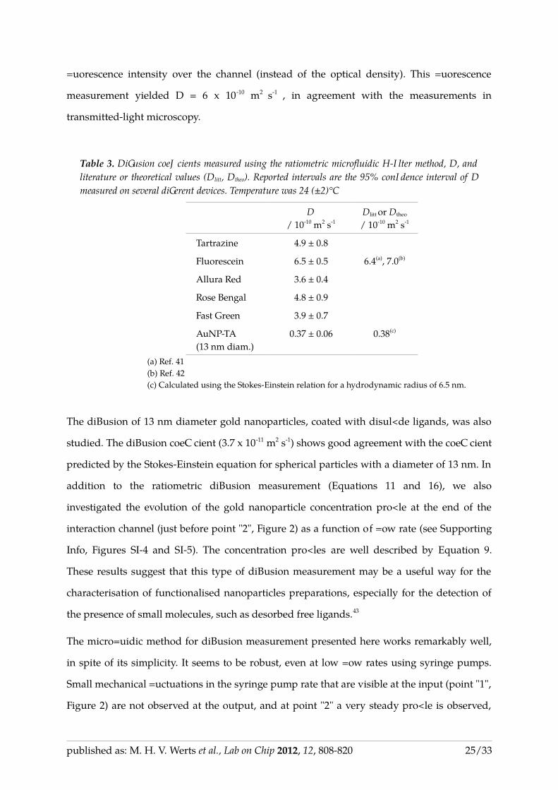
fluorescence intensity over the channel (instead of the optical density). This fluorescence
measurement yielded D = 6 x 10⁻¹⁰ m2 s-1 , in agreement with the measurements in
transmitted-light microscopy.
Table 3. Diffusion coefficients measured using the ratiometric microfluidic H-filter method, D, andliterature or theoretical values (Dlitt, Dtheo). Reported intervals are the 95% confidence interval of Dmeasured on several different devices. Temperature was 24 (±2)°C
D/ 10-10 m2 s-1
Dlitt or Dtheo
/ 10-10 m2 s-1
Tartrazine 4.9 ± 0.8
Fluorescein 6.5 ± 0.5 6.4(a), 7.0(b)
Allura Red 3.6 ± 0.4
Rose Bengal 4.8 ± 0.9
Fast Green 3.9 ± 0.7
AuNP-TA(13 nm diam.)
0.37 ± 0.06 0.38(c)
(a) Ref. 41 (b) Ref. 42 (c) Calculated using the Stokes-Einstein relation for a hydrodynamic radius of 6.5 nm.
The diffusion of 13 nm diameter gold nanoparticles, coated with disulfide ligands, was also
studied. The diffusion coefficient (3.7 x 10⁻¹¹ m2 s-1) shows good agreement with the coefficient
predicted by the Stokes-Einstein equation for spherical particles with a diameter of 13 nm. In
addition to the ratiometric diffusion measurement (Equations 11 and 16), we also
investigated the evolution of the gold nanoparticle concentration profile at the end of the
interaction channel (just before point "2", Figure 2) as a function of flow rate (see Supporting
Info, Figures SI-4 and SI-5). The concentration profiles are well described by Equation 9.
These results suggest that this type of diffusion measurement may be a useful way for the
characterisation of functionalised nanoparticles preparations, especially for the detection of
the presence of small molecules, such as desorbed free ligands.43
The microfluidic method for diffusion measurement presented here works remarkably well,
in spite of its simplicity. It seems to be robust, even at low flow rates using syringe pumps.
Small mechanical fluctuations in the syringe pump rate that are visible at the input (point "1",
Figure 2) are not observed at the output, and at point "2" a very steady profile is observed,
published as: M. H. V. Werts et al., Lab on Chip 2012, 12, 808-820 25/33

that reliably changes as a function of overall flow rate. Since measurement is done at the end
of the channel (at relatively long mixing times) complicating factors are likely smoothed out,
e.g. with Taylor-Aris dispersion smoothing out the Poiseuille flow profile. Comparison of the
"Fourier-based" analysis used in this work and the "erf-based" (Equation 8) analysis shows
that the latter works mainly at short mixing times (i.e. at the input of the H-filter/T-sensor),
and the former is very effective at moderate to long mixing times (see Supporting Info, Figure
SI-3).
Perhaps the fluidic implementation may be improved using flow focussing techniques for
reducing wall effects.6 However, the current implementation using ratiometric measurement
of overall concentrations may be much less sensitive to wall effects as the overall response is
averaged out, and the long flow length favorises volume effects over wall effects.
5 Multicomponent analysis: Characterisation of a passive mixer and a gradient generator
As an illustration of the multicomponent concentration mapping capability of colour
transmitted light microscopy we studied two typical microlfluidic systems: a passive mixer
based on the staggered herringbone motif35 and a gradient generator.21,44,45
A panoramic microscopy image of the staggered herringbone mixer (SHM) was constructed
from individual images taken at different positions (see Supporting Info, Figure SI-6). The
mixer was operated mixing 0.9 mM fast green and 4.6 mM tartrazine ('blue + yellow =
green'), both in PBS. From the individual images we extracted the concentration profiles of
each dye before mixing, and after 2, 4, 6, 8 and 10 SHM cycles (Figure 6). Our measurements
show that after 10 mixing cycles the concentration profiles of both dyes are completely flat.
published as: M. H. V. Werts et al., Lab on Chip 2012, 12, 808-820 26/33

Figure 6. Evolution of the central part of the concentration profiles of Fast Green (top) andTartrazine (bottom) in a staggered herringbone mixing device (see also Supporting Info for an imageof the device) monitored using full-colour transmitted light microscopy and multicomponentanalysis. Profiles are shown before ("0x") and after 2, 4, 6, 8, and 10 mixing cycles. Total flow rate in100 µm high, 200 µm wide mixing channel: 14 µl min-1.
It is interesting to compare the transmitted-light profiles (Figure 6), which are optical
densities that are averaged in the direction of light propagation (the "z" direction, from
channel top to channel bottom), to (single component) confocal microscopy images
previously taken on an SHM that resolve this vertical concentration profile. We then see that
the transmitted-light profiles indeed follow (at least semi-quantitatively) the averages along
the vertical axis of these confocal images.
In addition to the passive chaotic mixer, we also studied a chemical gradient generator under
development for cell studies. Cell toxicology assays are a common application for
microfluidic gradient generators.44,45 They can also be used as a microfluidic component in
the development of chemical micro-reactors for analytical or biomedical applications. Based
on well-controlled successive dilutions of initial stock solutions in a large microarray,
gradients are generated with the use of multiple T-channels.37 Several channels are combined
in order to obtain the desired concentration gradient.40
published as: M. H. V. Werts et al., Lab on Chip 2012, 12, 808-820 27/33

The device shown in Figure 7 is a simple pyramidal architecture designed for achieving a
well-controlled gradient of two stock solutions, distributed over 9 perfusion chambers for cell
studies. The device has been designed with a channel height of 75 µm. Each T-channel has a
length of mixing of 5 mm and a width of 50 µm. The panoramic image is composed of 31
individual microscope images, each of which has been flat-field corrected (Equation 2).
With the homogenised illumination it is now straightforward to extract concentration
profiles. Two of such profiles are shown in Figure 7. Profiles "A" show the profiles at an
intermediate stage, where four gradient steps have been generated. Interestingly, as is
particularly clear from the encircled part of the profiles, the mixing of the input streams is
not entirely complete at the flow rate used. As a result, the middle chamber at the output
(profiles "B") does not have exactly a 50:50 mixture of the inital solutions. This is not
immediately clear from the overall image, and is only revealed after quantitative
determination of the two-component concentration profiles. The device should be operated
at a lower flow rate in order to achieve a perfect gradient over the cell perfusion chambers.
Figure 7. Left: Panoramic picture (multiple images taken using a 2.5x NA 0.07 objective) of agradient generator (channel height 75 µm) that generates a gradient distributed over 9 perfusionchambers. The input solutions are Tartrazine/PBS and Fast Green/PBS. Right: normalizedconcentration profiles for Tartrazine (yellow) and Fast Green (blue) determined usingmulticomponent analysis of the colour optical density profiles. Total flow rate 4 µl min-1, which isslightly too high to ensure complete mixing leading to small deviations from ideality, illustrated bythe encircled zone of Profiles "A".
published as: M. H. V. Werts et al., Lab on Chip 2012, 12, 808-820 28/33

6 Conclusion
The possibility of implementing quantitative multicomponent concentration measurements
in microfluidic systems using transmitted light microscopy and full colour imaging has been
demonstrated, in spite of the non-monochromatic nature of the Bayer colour filters used in
(digital) cameras, which was expected to complicate application of Beer-Lambert law. The
methodology presented in this work will help more thorough characterisation of
microfluidic architectures with relatively simple equipment. Additionally, it may help
implementation of simple detection schemes in (bio)microsystems, when used with coloured
indicators (pH, metals, redox, proteins...). A set of coloured solutions of well-defined
composition for microfluidics is proposed, with the trio Fast Green-Amaranth-Tartrazine
(cyan-magenta-yellow) being well-suited for use with RGB (red-green-blue) cameras. The
methodology may be extended to other dye systems, such as acid-base or metal indicators
(and light-absorbing nanoparticles, as demonstrated).
The implementation of quantitative dye concentration measurements using a colour camera
enabled us to develop and validate a simplified ratiometric method for the determination of
diffusion coefficients using an H-filter architecture. This ratiometric method simplifies and
greatly extends the scope of diffusion measurements in microfluidic systems, that can be
further extended to include non-optical (e.g. electroanalytical46) detection methods.
Acknowledgments
Financial support from ERANET-NanoSciences (project MOLIMEN) and the Agence
Nationale de la Recherche (program JCJC2010, project COMONSENS) are gratefully
acknowledged.
Experimental section
Spectroscopy and microscopy
Spectroscopic and digital imaging data were analysed using home-written software based on
the Scipy (0.7.0), Numpy (1.3.0) and Matplotlib (0.99.1.1) libraries for the Python
programming language (version 2.6.5), on Windows XP, Mac OS X or GNU/Linux systems.
published as: M. H. V. Werts et al., Lab on Chip 2012, 12, 808-820 29/33

UV/vis absorption spectrometric measurements were performed using an optical fiber-based
system (OceanOptics, USA) incorporating a USB4000-VIS-NIR CCD spectrometer and an LS-
1 tungsten-halogen light source equipped with a BG34 colour correction filter. The data
reported are based on the dilution series of at least three independently prepared solutions.
The maximum values of the absorption spectra, and their spectral position, were obtained
from fitting a parabola through the experimental spectra in a small window (+/- 5 nm)
centered around the numerical maximum (which is not necessarily the maximum of the
absorption band due to noise).
Transmitted light microscopy was performed on a Leica DMIRB inverted microscope, with a
tungsten-halogen light source with "daylight" (DLF) correction filter and a Hitachi KP-D50
CCD colour camera with Pinnacle frame grabber. For measurement of concentration profiles
inside a single fluidic channel or concentration ratios between two parallel channel channels,
a 10x (NA 0.22) CPlan objective was used. For the panoramic images, a 2.5x (NA 0.07) NPlan
objective was employed. For comparison, several experiments were repeated on a Olympus
IX71 microscope with a low-cost Thorlabs DCC-1645-C CMOS colour camera, with either a
10x (NA 0.30) CPlan-Fl objective, or a 2x (NA 0.06) PlanN objective.
Microfabrication and device operation
Microfluidic channels were moulded into polydimethylsiloxane (PDMS, General Electric
RTV615) using SU-8 (Microchem, SU8-2100) moulds defined on 2" silicon wafers by standard
photolithographic processes. After cross-linking (2h @ 75°C), the PDMS slab was attached to
cleaned microscope glass slides (25mm x 75mm) using low pressure air plasma bonding
(Harrick Plasma Cleaner PDC-002, 1 minute). Cleaning of the glass slides involved rubbing
with isopropanol (iPrOH) and cleanroom wipes followed by sonication in 1% Hellmanex II
(Hellma) at 35°C, thorough rinsing with ultrapure water, followed by iPrOH, drying in a
nitrogen jet and subsequently in a stove at 70°C, ending with 15 minutes in the plasma
cleaner.
Microfluidic systems were operated with Aladdin (WPI Europe, Hertfordshire, UK) or
Harvard (Harvard Apparatus, Holliston MA, USA) syringe pumps and 250 µl...1000 µl glass
precision syringes (SGE Europe, Milton Keynes, UK). The fluids were supplied to the devices
published as: M. H. V. Werts et al., Lab on Chip 2012, 12, 808-820 30/33

using ETFE Tefzel tubing (Cluzeau, Sainte-Foy-La-Grande, France) containing in-line filters
(2 µm pore diameter, Cluzeau).
Gold nanoparticles
Thiooctic acid-capped gold nanoparticles of 13 nm diameter (AuNP-TA) were prepared by
adding a solution of thiooctic acid to a solution of excess citrate-stabilised gold nanoparticles.
The excess citrate-stabilised gold sol was prepared according to the well-known Frens-
Turkevich method47,48 following the recipe in Ref. 49. The citrate gold sol was found to have a
concentration of 4.2 x 10⁻⁹ M in gold nanoparticles, using UV-visible spectroscopy (εpart = 2.4 x
108 M-1 cm-1 for 13 nm diameter citrate AuNP).32
An aqueous solution containing 2.4 mM NaOH and 2.4 mM DL-thiooctic acid was prepared,
and 2.5 ml of this solution was added dropwise to 150 ml of a vigourously stirred gold sol.
After stirring for another 30 minutes, the solution was stored in the dark overnight. The
solution was concentrated by several cycles of centrifugation (9 700 x g, 10 000 rpm, 10 min.,
Hettich Mikro 220r), removal of supernatant (90% of the volume) followed by replacement of
the removed supernatant by additional nanoparticle solution. The concentrate had a final
particle concentration of 7.3 x 10⁻⁷ M. The concentrate was then further purified by diluting it
10 times using 1 mM aqeous NaOH, followed by centrifugation (9 700 x g, 10 min.), and
removal of supernatant (90% of the volume). The pellet was finally diluted 2.5 times using 1
mM aqueous NaOH, to give a nanoparticle solution at 2.9 x 10 -7 M. Before disposal, spent
nanoparticle solutions were exposed to gold etchant (Transene Gold Etchant TFA, which
converts the nanoparticles into gold ions, and thus removes the nanoparticulate nature of the
waste).49
References1 I. Broadwell, P. D. I. Fletcher, S. J. Haswell, T. McCreedy and X. L. Zhang, Quantitative 3-dimensional
profiling of channel networks within transparent 'lab-on-a-chip' microreactors using a digital imagingmethod, Lab Chip, 2001, 1, 66-71.
2 P. D. I. Fletcher, S. J. Haswell and X. L. Zhang, Electrokinetic control of a chemical reaction in a lab-on-a-chipmicro-reactor: measurement and quantitative modelling, Lab Chip, 2002, 2, 102-112.
3 D. C. Leslie, B. A. Melnikoff, D. J. Marchiarullo, D. R. Cash, J. P. Ferrance and J. P. Landers, A simple methodfor the evaluation of microfluidic architecture using flow quantitation via a multiplexed fluidic resistancemeasurement, Lab Chip, 2010, 10, 1960-1966.
4 C. Hsu and A. Folch, Spatio-temporally-complex concentration profiles using a tunable chaotic micromixer,Appl. Phys. Lett., 2006, 89, 144102.
published as: M. H. V. Werts et al., Lab on Chip 2012, 12, 808-820 31/33

5 A. E. Kamholz, E. A. Schilling and P. Yager, Optical measurement of transverse molecular diffusion in amicrochannel, Biophys. J., 2001, 80, 1967-72.
6 M. S. Munson, K. R. Hawkins, M. S. Hasenbank and P. Yager, Diffusion based analysis in a sheath flowmicrochannel: the sheath flow T-sensor, Lab Chip, 2005, 5, 856-62.
7 G. M. Walker, N. Monteiro-Riviere, J. Rouse and A. T. O'Neill, A linear dilution microfluidic device forcytotoxicity assays, Lab Chip, 2007, 7, 226.
8 J. Q. Wu and J. Pawliszyn, Dual detection for capillary isolelectric focusing with refractive index gradient andabsorption imaging detectors, Anal. Chem., 1994, 66, 867-873.
9 C. Rothmann, A. M. Cohen and Z. Malik, Chromatin condensation in erythropoiesis resolved by multipixelspectral imaging: Differentiation versus apoptosis, J. Histochem. Cytochem., 1997, 45, 1097-1108.
10 J. Thigpen, F. A. Merchant and S. K. Shah, Photometric calibration for quantitative spectral microscopy undertransmitted illumination, J. Microscopy, 2010, 239, 200-214.
11 B. P. Binks, Z. G. Cui and P. D. I. Fletcher, Optical microscope absorbance imaging of carbon blacknanoparticle films at solid and liquid surfaces, Langmuir, 2006, 22, 1664-1670.
12 T. A. Everett and D. A. Higgins, Electrostatic self-assembly of ordered perylene-diimide/polyelectrolytenanofibers in fluidic devices: from nematic domains to macroscopic alignment, Langmuir, 2009, 25, 13045-13051.
13 N. Kakuta, Y. Fukuhara, K. Kondo, H. Arimoto and Y. Yamada, Temperature imaging of water in amicrochannel using thermal sensitivity of near-infrared absorption, Lab Chip, 2011, DOI: 10.1039/c1lc20261h.
14 G. C. Y. Chan and W. T. Chan, Beer's law measurements using non-monochromatic light sources - a computersimulation, J. Chem. Ed., 2001, 78, 1285-1288.
15 A. E. Kamholz, B. H. Weigl, B. A. Finlayson and P. Yager, Quantitative analysis of molecular interaction in amicrofluidic channel: the T-sensor, Anal. Chem., 1999, 71, 5340-7.
16 B. H. Weigl and P. Yager, Microfluidics - Microfluidic diffusion-based separation and detection, Science, 1999,283, 346-347.
17 J. P. Brody and P. Yager, Diffusion-based extraction in a microfabricated device, Sens. Actuators A, 1997, 58, 13-18.
18 T. M. Squires and S. R. Quake, Microfluidics: fluid physics at the nanoliter scale, Rev. Mod. Phys., 2005, 77, 977-1026.
19 J. L. Osborn, B. Lutz, E. Fu, P. Kauffman, D. Y. Stevens and P. Yager, Microfluidics without pumps: reinventingthe T-sensor and H-filter in paper networks, Lab Chip, 2010, 10, 2659.
20 A. Persat, R. D. Chambers and J. G. Santiago, Basic principles of electrolyte chemistry for microfluidicelectrokinetics. Part I: Acid-base equilibria and pH buffers, Lab Chip, 2009, 9, 2437-53.
21 G. A. Cooksey, C. G. Sip and A. Folch, A multi-purpose microfluidic perfusion system with combinatorialchoice of inputs, mixtures, gradient patterns, and flow rates, Lab Chip, 2009, 9, 417.
22 C. Neils, Z. Tyree, B. Finlayson and A. Folch, Combinatorial mixing of microfluidic streams, Lab Chip, 2004, 4,342.
23 O. Valdes-Aguilera and D. C. Neckers, Aggregation phenomena in xanthene dyes, Acc. Chem. Res., 1989, 22,171-177.
24 C. Grotzinger, D. Burget, P. Jacques and J. P. Fouassier, Visible light induced photopolymerization: speedingup the rate of polymerization by using co-initiators in dye/amine photoinitiating systems, Polymer, 2003, 44,3671-3677.
25 P. Gottschalk, J. Paczkowski and D. C. Neckers, Factors influencing the quantum yields for rose bengalformation of singlet oxygen, J. Photochem., 1986, 35, 277-281.
26 S. Y. Lin, Y. T. Tsai, C. C. Chen, C. M. Lin and C. H. Chen, Two-step functionalization of neutral and positivelycharged thiols onto citrate-stabilized Au nanoparticles, J. Phys. Chem. B, 2004, 108, 2134-2139.
27 P. K. Jain, X. H. Huang, I. H. El-Sayed and M. A. El-Sayed, Noble metals on the nanoscale: optical andphotothermal properties and some applications in imaging, sensing, biology, and medicine, Acc. Chem. Res.,2008, 41, 1578-1586.
published as: M. H. V. Werts et al., Lab on Chip 2012, 12, 808-820 32/33
28 J. Yguerabide and E. E. Yguerabide, Light-scattering submicroscopic particles as highly fluorescent analogsand their use as tracer labels in clinical and biological applications: I. Theory, Anal. Biochem., 1998, 262, 137-156.
29 J. Yguerabide and E. E. Yguerabide, Light-scattering submicroscopic particles as highly fluorescent analogsand their use as tracer labels in clinical and biological applications: II. Experimental characterization, Anal.Biochem., 1998, 262, 157-176.
30. G. T. Hermanson. Bioconjugate Techniques (Academic Press, 1996), chapter 14.31 J. C. Love, L. A. Estroff, J. K. Kriebel, R. G. Nuzzo and G. M. Whitesides, Self-assembled monolayers of
thiolates on metals as a form of nanotechnology, Chem. Rev., 2005, 105, 1103-1169.32 N. Nerambourg, R. Praho, M. H. V. Werts, D. Thomas and M. Blanchard-Desce, Hydrophilic monolayer-
protected gold nanoparticles and their functionalisation with fluorescent chromophores, Int. J. Nanotechnol.,2008, 5, 722-740.
33 R. Samy, T. Glawdel and C. L. Ren, Method for microfluidic whole-chip temperature measurement using thin-film poly(dimethylsiloxane)/rhodamine B, Anal. Chem., 2008, 80, 369-375.
34 B. E. Bayer, Color imaging array, U. S. Patent, 1976, US 3,971,065.35 A. D. Stroock, S. K. W. Dertinger, A. Ajdari, I. Mezić, H. A. Stone and G. M. Whitesides, Chaotic mixer for
microchannels, Science, 2002, 295, 647 -651.36. P. Tabeling. Introduction to microfluidics (Oxford University Press, Oxford, UK, 2005), chapter 3, p. 142.37 N. L. Jeon, S. K. W. Dertinger, D. T. Chiu, I. S. Choi, A. D. Stroock and G. M. Whitesides, Generation of
Solution and Surface Gradients Using Microfluidic Systems, Langmuir, 2000, 16, 8311-8316.38 M. Bonn, H. J. Bakker, G. Rago, F. Pouzy, J. R. Siekierzycka, A. M. Brouwer and D. Bonn, Suppression of
proton mobility by hydrophobic hydration, J. Am. Chem. Soc., 2009, 131, 17070-17071.39 C. N. Baroud, F. Okkels, L. Ménétrier and P. Tabeling, Reaction-diffusion dynamics: Confrontation between
theory and experiment in a microfluidic reactor, Phys. Rev. E, 2003, 67, 060104.40 Y. Wang, T. Mukherjee and Q. Lin, Systematic modeling of microfluidic concentration gradient generators, J.
Micromech. Microeng., 2006, 16, 2128-2137.41 P. Galambos and F. K. Forster, Micro-fluidic diffusion coefficient measurement, µTAS, 1998, 189-191.42 R. K. Jain, Transport of macromolecules in tumor microcirculation, Biotechnol. Prog., 1985, 1, 81-94.43 M. Loumaigne, R. Praho, D. Nutarelli, M. H. V. Werts and A. Débarre, Fluorescence correlation spectroscopy
reveals strong fluorescence quenching of FITC adducts on PEGylated gold nanoparticles in water and thepresence of fluorescent aggregates of desorbed thiolate ligands, Phys. Chem. Chem. Phys., 2010, 12, 11004-11014.
44 N. L. Jeon, H. Baskaran, S. K. W. Dertinger, G. M. Whitesides, L. Van De Water and M. Toner, Neutrophilchemotaxis in linear and complex gradients of interleukin-8 formed in a microfabricated device, Nat. Biotech.,2002, 20, 826-830.
45 A. Tirella, M. Marano, F. Vozzi and A. Ahluwalia, A microfluidic gradient maker for toxicity testing ofbupivacaine and lidocaine, Toxicol. in Vitro, 2008, 22, 1957-1964.
46 D. Quinton, A. Girard, L. To Thi Kim, V. Raimbault, L. Griscom, F. Razan, S. Griveau and F. Bedioui , On-chipmulti-electrochemical sensor array platform for simultaneous screening of nitric oxide and peroxynitrite, LabChip, 2011, 11, 1342-1350 .
47 J. Turkevich, P. C. Stevenson and J. Hillier, A study of the nucleation and growth process in the synthesis ofcolloidal gold, Discuss. Faraday Soc., 1951, 11, 55-75.
48 G. Frens, Controlled nucleation for the regulation of the particle size in monodisperse gold suspensions,Nature Phys. Sci., 1973, 241, 20-22.
49 J. R. G. Navarro, M. Plugge, M. Loumaigne, A. Sanchez Gonzalez, B. Mennucci, A. Débarre, A. M. Brouwerand M. H. V. Werts, Probing the interactions between disulfide based ligands and gold nanoparticles using afunctionalised fluorescent perylene-monoimide dye, Photochem. Photobiol. Sci., 2010, 9, 1042-1054.
published as: M. H. V. Werts et al., Lab on Chip 2012, 12, 808-820 33/33