quantitative it portfolio managementx/ipm/ipm.pdfquantitative it portfolio management—the subject...
TRANSCRIPT
Science of Computer Programming 45 (2002) 1–96www.elsevier.com/locate/scico
Quantitative IT portfolio management
C. VerhoefFree University of Amsterdam, Department of Mathematics and Computer Science,
De Boelelaan 1081a, 1081 HV Amsterdam, The Netherlands
Received 19 April 2002; received in revised form 10 July 2002; accepted 15 July 2002
Abstract
We present a quantitative approach for IT portfolio management. This is an approach thatCMM level 1 organizations can use to obtain a corporate wide impression of the state of theirtotal IT portfolio, how IT costs spent today project into the budgets of tomorrow, how toassess important risks residing in an IT portfolio, and to explore what-if scenarios for futureIT investments. Our quantitative approach enables assessments of proposals from business units,risk calculations, cost comparisons, estimations of TCO of entire IT portfolios, and more. Ourapproach has been applied to several organizations with annual multibillion dollar IT budgetseach, and has been instrumental for executives in coming to grips with the largest productionfactor in their organizations: information technology.c© 2002 Elsevier Science B.V. All rights reserved.
Keywords: IT portfolio; IT portfolio management; IT portfolio database; Cost allocation formulas; SeismicIT impulse; Operational cost tsunami; ROI threshold quavering; IT portfolio risk; IT portfolio exposure;Cost allocation distribution; Rayleigh distribution; Sech square distribution; Damped sine distribution;Generalized � distribution; Generalized F distribution; Total cost of ownership; Cost–time analysis;Lifetime analysis; Failure time analysis; Survival function; Hazard rate
1. Introduction
It is known from extensive research being conducted by the former CIO of the USDepartment of Defense, Paul A. Strassmann [119,120,123,124], that there is no relationbetween information management per employee and return on shareholder equity. Alsothere is no relation between proCts and annual IT spending. So he shows that thereis no direct relation between spending on computers, proCts or productivity. Indeed,there are companies—in the same industry—each spending about the same on IT ofwhich the one makes high proCts, and the other makes huge losses [125]. This leads to
E-mail address: [email protected] (C. Verhoef).
0167-6423/02/$ - see front matter c© 2002 Elsevier Science B.V. All rights reserved.PII: S0167 -6423(02)00106 -5
2 C. Verhoef / Science of Computer Programming 45 (2002) 1–96
shotgun patterns showing the absence of correlations between any kind of return andthe intensity of IT investments. The only vague correlation that Strassmann ever foundwas that when from two comparable enterprises one is spending slightly less than theother, the less spending organization is doing slightly better. This loose correlationleads one to suspect that governance of IT investments aids in creating value with ITinstead of destroying proCts. Indeed a continuous stream of reports on value destructioneventually led to the so-called Clinger Cohen Act [46], explicitly stating that the CIO’sjob is critical to ensure that the mandates of the Clinger Cohen Act are implemented.This includes that IT investments (we quote from [46]):
ReIect a portfolio management approach where decisions on whether to invest inIT are based on potential return, and decisions to terminate or make additionalinvestments are based on performance much like an investment broker is measuredand rewarded based on managing risk and achieving results
The US Government has to come to grips with IT portfolio management: anyacquisition program for a mission critical or mission essential IT system for the USGovernment must be developed in accordance with the Clinger Cohen Act of 1996.To that end, the US General Accounting OJce proposed a framework for initiat-ing and maturing IT investment management [90]. But also outside the public sectorthere is increasing interest in deploying IT portfolio management. In a 2002 surveyamong 400+ top IT executives 60% reported an increase in the level of pressure toprove ROI on IT investments. But 70% believe their metrics do not fully capture thevalue of IT, and nearly half lack conCdence in their ability to accurately calculateROI on IT investments [71]. The Federal CIO Council summarized in 2002 the Crstlessons learned for IT portfolio management. The report does not mention quantitativeapproaches to manage IT portfolios [24]. This report should be seen complimentaryto our work: the lessons learned provide a Crst insight in implementing qualitativeaspects of IT portfolio management in organizations. This paper deals with quantitativeIT portfolio management. In particular, we consider quantitative aspects of IT devel-opment, operations, maintenance, enhancement, and renovation for bespoke softwaresystems. For other possible contents of an IT portfolio, such as license managementfor COTS systems, processing hardware infrastructure, network equipment, and so on,tools and techniques are available to deal with them. For instance, several companiesare specialized in license management, and hardware=network infrastructure investmentissues are better understood than software cost issues. In addition, Strassmann indicatesthat the focus on hardware costs is wrong: on the average this accounts for 5% of thelife-cycle cost for information management so hardware is not the dominating factor[122, p. 409]. Bespoke software is our main focus. To the best of our knowledgequantitative IT portfolio management—the subject of this paper—is a terra incognita.
Executives of large organizations with substantial IT budgets learned the hard waythat spending more is not the winning strategy. Some of them realized that after a longstring of staggering IT investments plus their challenges, they must start to controltheir IT portfolios. Most executives consider IT spending as a black hole: no matterhow much resources are thrown at IT, there is no clear justiCcation of returns—ITis on top of the executives. We consulted executives about a variety of investment
C. Verhoef / Science of Computer Programming 45 (2002) 1–96 3
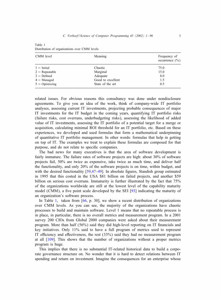
Table 1Distribution of organizations over CMM levels
CMM level Meaning Frequency ofoccurrence (%)
1 = Initial Chaotic 75.02 = Repeatable Marginal 15.03 = DeCned Adequate 8.04 = Managed Good to excellent 1.55 = Optimizing State of the art 0.5
related issues. For obvious reasons this consultancy was done under nondisclosureagreements. To give you an idea of the work, think of company-wide IT portfolioanalyses, assessing current IT investments, projecting probable consequences of majorIT investments for the IT budget in the coming years, quantifying IT portfolio risks(failure risks, cost overruns, underbudgeting risks), assessing the likelihood of addedvalue of IT investments, assessing the IT portfolio of a potential target for a merge oracquisition, calculating minimal ROI threshold for an IT portfolio, etc. Based on theseexperiences, we developed and used formulas that form a mathematical underpinningof quantitative IT portfolio management. In other words: formulas that help in gettingon top of IT. The examples we treat to explain these formulas are composed for thatpurpose, and do not relate to speciCc companies.
The bad news for many executives is that the area of software development isfairly immature. The failure rates of software projects are high: about 30% of softwareprojects fail, 50% are twice as expensive, take twice as much time, and deliver halfthe functionality, and only 20% of the software projects is on time, within budget, andwith the desired functionality [59,47–49]. In absolute Cgures, Standish group estimatedin 1995 that this costed in the USA $81 billion on failed projects, and another $59billion on serious cost overruns. Immaturity is further illustrated by the fact that 75%of the organizations worldwide are still at the lowest level of the capability maturitymodel (CMM), a Cve point scale developed by the SEI [93] indicating the maturity ofan organization’s software process.
In Table 1, taken from [66, p. 30], we show a recent distribution of organizationsover CMM levels. As you can see, the majority of the organizations have chaoticprocesses to build and maintain software. Level 1 means that no repeatable process isin place, in particular, there is no overall metrics and measurement program. In a 2001survey 200 CIOs from Global 2000 companies were asked about their measurementprogram. More than half (56%) said they did high-level reporting on IT Cnancials andkey initiatives. Only 11% said to have a full program of metrics used to representIT eJciency and eOectiveness, the rest (33%) said they had no measurement programat all [109]. This shows that the number of organizations without a proper metricsprogram is huge.
This implies that there is no substantial IT-related historical data to build a corpo-rate governance structure on. No wonder that it is hard to detect relations between ITspending and return on investment. Imagine the consequences for an enterprise whose
4 C. Verhoef / Science of Computer Programming 45 (2002) 1–96
Cnancial department is anarchic. The problem for executives of level 1 organizationswho want to get in control of their software portfolios now, becomes then very com-pelling. For, how to measure anything at the corporate level if there is no relevant dataavailable to accumulate management information from?
Our approach to quantitative IT portfolio management provides you with insightin an IT portfolio, even in the case of level 1 organizations. A level 1 organizationhas to compensate for the lack of historical information by utilizing and deployingbenchmark information. We developed a set of mathematical formulas based on publicbenchmark information to quantitatively manage IT portfolios. When you have histor-ical data and can establish internal benchmarks, you can use these to instantiate ourformulas.
The simplest formulas can be handled by spread sheets or a pocket calculator. Forthe more involved analyses, a scientiCc calculator like the HP49G or the TI89 canbe used. For advanced issues, it is convenient to use statistical=mathematical packagesranging from spread sheets with plugins, to packages like SAS [31], SPSS [114], SPlus[129,73], Matlab [81], Maple [135], or Mathematica [132].
The set of formulas has shown to be a useful executive’s armature to analyze,assess, and control IT portfolio issues, to counteract bombardments of jargon riddenempty promises by the trade press, software vendors, consultants, or proposals fromtheir own internal IT departments. These formulas comprise relevant benchmarked IT-project information, which is often not provided to the executives, if only since theIT jargoneers have no clue how to come up with the information themselves. To usethese formulas successfully you do not need to acquire extensive IT knowledge: wehave completely hidden this aspect (but it is incorporated via benchmark informa-tion). The typical academic qualiCcations of the executive staO that we dealt with hasan MBA combined with an M.Sc. or Ph.D. in an exact science. Think of economy,econometrics, astrophysics, experimental and theoretical physics, chemistry, biochem-istry, mathematics, Cnancial mathematics, business mathematics, statistics, biostatistics,electrical engineering, and so on. We encountered hardly ever educational backgroundswith a strong focus on IT, and when executives had such a background, they werecombined with degrees in other exact sciences. Executive staO who were exposed toour formulas could understand them, could work with them, and were helped by themin that they lost their naivity with respect to IT decision making.
Does IT portfolio management pay oO? In one organization the initial investmentin research and development, plus the inevitable errors made during thisendeavor, were about $250 000 dollar. An additional $120 000 dollar were neededfor training. In this organization, the eOort to keep the IT portfolio database up todate costs about $50 000 dollar. The return is depending on the size of the IT port-folio measured in dollars. For a 500 million dollar IT portfolio direct cost savingsper annum of 3–5% of the total portfolio value were established by betterdecision making: killing bad performing projects, mitigating risks, abandoning nega-tive ROI investments, removing system redundancies, etc. As reported in CIOMagazine: just compiling an IT portfolio database saved one company $3 million andanother company $4:5 million because the holistic IT portfolio view enabled them tospot redundancies [5]. Those redundancies could be eliminated, reaping the beneCts.
C. Verhoef / Science of Computer Programming 45 (2002) 1–96 5
For organizations above level 1, the accuracy of the underlying benchmarks can besigniCcantly improved, and the underlying mathematics as presented in this paper canbe instantiated accordingly. So, the principles of quantitative IT portfolio managementremain unchanged. We will for the rest of this paper assume the level 1 situation sothat the majority of current organizations can apply our results, yet when appropriatepoint out how our work applies to CMM 2+ levels.
2. How to tell a program from a security
In the 1970s, it was hard for many to grasp the diOerence between hardware andsoftware maintenance, and Leslie Lamport explained this in a short note [74] entitledHow to tell a program from an automobile. We borrowed this title to explain thatyou cannot simply apply security portfolio management to IT portfolios.
As far as we know there is no related work reported on in the realm of quantitativeIT portfolio management, although many of us think that security portfolio managementis strongly related. The reason is that the goals of both security portfolio managementand IT portfolio management are largely identical. We will show that the means toreach this common goal do not coincide.
A lot of important work has been done in quantitative security portfolio manage-ment. And at Crst sight it seems a promising idea to support the quantitative part ofIT portfolio management with the theory that 1990 Nobel Laureate Harry Markowitzdeveloped on security portfolio management [80]. We heard this from several exec-utives who were exposed to his work, but also the US Federal CIO council seemsto play with this idea [24]. Moreover, the trade-press quotes people who think thatapplying this so-called modern portfolio theory is the noble endgame in IT port-folio management [5]. But what is this theory about? In the words of Markowitz[80, p. 205]:
Thus, in large part, this monograph is a discussion of the relationships and proce-dures by which information about securities is transformed into conclusions aboutportfolios.
The current paper is also a discussion of the relationships and procedures bywhich information about IT systems is transformed into conclusions about ITportfolios.
Markowitz investigated the available information about securities, the questions thatneed an answer and found the appropriate mathematical techniques to provide sen-sible answers to the problems. In the current paper we do exactly the same: wegather and investigate the data that is commonly available on IT projects, we in-vestigated the questions that need an answer, and by working on the answers, werelated the problems to the appropriate mathematical techniques to provide sensibleanswers.
Given these parallels, it may be hard for the Cnancial expert, who might neverhave been exposed to information technology, (by building, maintaining, operating,enhancing, or retiring IT) to tell the diOerence between a program and a security.
6 C. Verhoef / Science of Computer Programming 45 (2002) 1–96
Likewise, for the IT expert, who might never have been exposed to the nature ofsecurities (by selling them, buying them, comprising them into portfolios, or advisingothers about these issues), it might be hard to tell the diOerence as well. As oneexecutive put it [5]:
The cancellation rate of the largest IT projects exceeds the default rate on the worstjunk bonds. And the junk bonds have lots of [portfolio management tools] appliedto them. IT investments are huge, risky investments. It’s time we do [Markowitz’sportfolio management].
So they both are high risk investments, and another seeming parallel is implied. Inthe same article an IT portfolio manager said she had learned that some people argueagainst using modern portfolio theory since it cannot be overlaid exactly, and that themath is too diJcult [5]. But what kind of math is being used in Markowitz’s book[80]? As Markowitz states it [80, p. 186]:
The problem of maximizing expected return subject to linear constraints, [..] isa linear programming problem. [..] the problem of Cnding the portfolio whosesmallest [return at time t] is as large as possible can be formulated as a linearprogramming problem.
The nature of securities is that you can select them, you can calculate their historicalreturn, and based on these data you can use linear programming to calculate the optimalselection that maximizes expected return while minimizing variance by diversiCcation.The underlying mathematics is elementary linear algebra, plus elementary statistics, andthe use of standard linear programming techniques such as the simplex method. Whilethis is not immediately digestible for the uninitiated, the math is not inherently complex.So, we agree that the complexity of the math should not be an argument against usingmodern portfolio theory as proposed by Markowitz. This is obviously also supportedby the author of [5] given the supportive title of the article: Do the MATH.
But what about this overlay? The nature of securities is that you can invest anddisinvest in them and implement a decision without prohibitively large costs, and oftenin a matter of seconds. Modern portfolio theory essentially asserts that investing anddisinvesting at all times is enabled. The heart of security portfolio management is tomonitor, control, and optimize the security selection process.
The Y2K problem and Euro conversion problem have clearly shown that you cannotsimply junk IT systems, as is possible with underperforming securities. If you wouldhave applied modern portfolio theory to IT systems that were suOering from the Y2Kproblem, you should have sold them, and bought better performing ones. For a start,to whom would you sell an IT system, especially, an IT system whose best-before-dateis due? Maybe the competitor wants to buy them, if only to reverse engineer them toreveal your successful business rules, or the features that you cannot implement, sothey can get ahead of you. Obviously, this is not an option, but even throwing themaway, and restarting from scratch with new systems is not an option. For, IT is com-prising business knowledge, often accumulations of it for many years. And convertingsuch business knowledge into IT is a laborious, error-prone, and painful process, soabandoning all that valuable knowledge is like burning an entire proCtable security
C. Verhoef / Science of Computer Programming 45 (2002) 1–96 7
portfolio. Moreover, implementing such IT systems takes years of time. So the wholeidea that there would be a free selection process, that companies are totally free tochoose in which IT they want to invest, that organizations can abandon systems likejunking bonds, is not in accord with the realities of large software portfolios.
Let us give a typical example showing the nature of IT investments, and the free-dom to choose. Suppose you have a good idea, like a credit card, or an ATM. Bothinventions are IT intensive, and both ideas were implemented by leading Cnancial cor-porations with deep pockets. In the beginning, they created value for both themselves,and their customers. But then the competitors united and answered with commodi-tized shared credit cards and a shared ATM network—not sharing with the initiator ofcourse. While still creating value for the customers, this competitive answer destroyednot only the proCts for the initiators, but also the margins for the entire market. Thediscretionary IT investment, thus turned into a commodity, and now you cannot operatea Cnancial corporation without credit cards, or ATMs. They have become must-have’swhile the proCt margins are gone—in some cases you even make a loss because ofthem. So, you are not free to disinvest in credit cards or ATMs anymore, since theinnovation set oO within the industry and customers insist on these services. This issometimes called: creating value while destroying pro7ts as explained in detail for thebanking sector in [118]. But according to Markowitz’s portfolio theory, these are port-folios to disinvest in: they cost money and do not deliver any positive return. Again,Markowitz’s theory is here a bad advisor, because these types of projects are reallynon-discretionary.
Let us give another example to make this apparent. Once you opted for a particularoperating system and accompanying languages it is no longer the case that you caneasily switch. Once you select a technology for your IT, you cannot easily abandonit. In the words of Michael Porter: there are low entry barriers, but high exit barriers[97, p. 22]. IT systems often make essential use of the underlying operating systemidiosyncrasies, clarifying the prohibitively high switching costs. This is not the casewith securities. Also, people work with IT systems and they have to learn a new ITsystem, which is not the case for a security. So also the switching costs for usersof the IT systems are high. Moreover, switching to a diOerent computer languageor even another dialect is hardly possible for existing software assets [126]. Whenattempting to convert to another language, you also need to convert your IT personnelsuccessfully. A 2001 Gartner report shows that converting a Cobol developer to aprofessional Java developer has a chance of failure of about 60% [37, p. 22]. Alsoa change of technology implies often a change in business process. This has shownto be a challenge in itself, with a high failure rate [113]. So, information technologybecomes illiquid after a Crst selection as opposed to securities or other Cnancial assetsthat do have liquidity. Changing information technology bears large risks, is virtuallyimpossible both technically and organizationally, and takes huge amounts of time. Soagain in this situation, Markowitz’s portfolio theory is not an adequate tool to supportIT decision making.
Also the issue of diversiCcation is not simply transposed to the IT situation. In orderto mitigate risks, and stabilize expected portfolio return, a diverse security portfolio isa good idea, and Markowitz gives the underlying mathematical tools to optimize this
8 C. Verhoef / Science of Computer Programming 45 (2002) 1–96
situation. What does diversiCcation mean in the realm of IT? Should we refrain frommany similar systems and make the IT systems more diOerent? For instance, by usingmore languages, diOerent operating systems, a host of development and maintenancetools? For IT you often try to do the opposite: consolidate diOerent but similar sys-tems into a single overall system: a product line that deals with the variation pointsof the similar systems successfully [10,22]. Also standardization is a keyword in theIT branch: use only a few languages, a limited number of operating systems, anda few support tools. So it is not a good idea to diversify in a technical sense, be-cause of knowledge investment, transfer, complexity, etc. Apart from these technicalaspects, there is also a business aspect. If you are a company building integratedradar systems for warships, then you are building those, and not enterprise resourceplanning systems for the automotive industry. To implement both types of systems,you need a lot of domain knowledge of both areas, e.g., for the warships you need toknow about developing software under military regulations, whereas for the automotiveindustry entirely diOerent issues are at stake. It is simply not very productive to com-bine uncorrelated IT domains. So also here, you see that the notions that are naturaland relevant for security portfolio management are without rhyme or reason for ITportfolio management.
Another aspect is that for securities there is a rich body of historical information.In contrast, many IT systems lack all historical information, and an entire branchin software engineering—reverse engineering—is devoted to cope with this problem[20]. The information that is around, is out of date, since deployed IT systems arein continuous Iux, and IT developers are not stars in writing documentation. Whilethe value of a security may Iuctuate on the stock exchange, the object itself doesnot change a bit. So the nature of the available information is diOerent, the na-ture of the objects is totally diOerent, but also the relevant questions are diOerent.Markowitz’s modern portfolio theory focuses on selection as a tool to minimize risk,and maximize return, while IT portfolio management is not at all aboutselecting and abandoning. So modern portfolio theory as proposed by Markowitz isnot applicable at all to IT portfolio management. Therefore, we are not surprised toread in the same article that advocates the use of Modern Portfolio Theory (MPT) [5]:
Who’s using Markowitz’s Modern Portfolio Theory in IT? Not many.
Simply, because it is not applicable. Also in paper [3] it was observed that there areproblems with applying Markowitz’s modern portfolio theory:
However, we have not yet seen any example of a substantial software project actu-ally using these techniques to help in their decision making process. We attributethis to the fact that obtaining economic data in software projects is much harderthan in Cnancial markets from where these techniques have been borrowed.
The idea that the data is the problem is erroneous, as we will see later on. Thereason is that the nature of software does not resemble the nature of a security.
Not only at the portfolio level but also at the single system level, people are think-ing of using modern portfolio theory. As an example, we quote a paper [16] inves-tigating the potential of using modern portfolio theory to guide decisions in software
C. Verhoef / Science of Computer Programming 45 (2002) 1–96 9
engineering:
We view each software activity as an investment opportunity (or security), thebeneCt from the activity as the return on investment, and the allocation problemas one of selecting the “optimal” portfolio of securities.
The paper claims that many decisions are ad hoc, and that portfolio selection couldimprove that situation. But then the subjects of selection should comply with modernportfolio theory. According to modern portfolio theory, you can lower risks with largenumbers of uncorrelated securities. We quote Markowitz [80, p. 102]:
We see that diversiCcation is extremely powerful when outcomes are uncorre-lated. [..] To understand the general properties of large portfolios we must con-sider the averaging together of large numbers of highly correlated outcomes. WeCnd that diversiCcation is much less powerful in this case. Only a limited reduc-tion in variability can be achieved by increasing the number of securities in aportfolio.
This leaves us to answer two questions: Is the amount of activities large? And, arethese activities uncorrelated? According to the activity-based cost estimation literature,there are at most 25 main activities in software development and deployment [66].Moreover, many of these activities are correlated, and if they are not correlated, thereis no free choice. Analysis, design, coding, testing, and operations: they are all stronglycorrelated. While you can drop analysis and design, it is already well-known that thisis not leading to the best possible IT systems. You do not need MPT to decide onthese issues. So MPT does not transpose that easily to the software world. The authorsof paper [16] admit that applying MPT did not work out in a subsequent paper [17]:
We have been attempting to apply Cnancial portfolio analysis techniques to thetask of selecting an application-appropriate suite of security technologies from thetechnologies available in the marketplace. The problem structures are suJcientlysimilar that the intuitive guidance is encouraging. However, the analysis techniquesof portfolio analysis assume precise quantitative data of a sort that we cannotrealistically expect to obtain for the security applications. This will be a com-mon challenge in applying quantitative economic models to software engineeringproblems, and we consider ways to address the mismatch.
The authors seem to think that MPT is the solution, and the problem is missing data.This is not true. 1 But their Cndings are conCrming the fact that 75% of the organi-zations is not mature with respect to their software development and deployment [66].
1 Apart from the arguments that we give in this paragraph, there is also a fundamental argument indicatingthat the premises for applying MPT are not fulClled. This argument may be less easy to comprehend uponCrst reading this paper. In [41, p. 293] it is stated that if the number of activities in a software project islarge, and if these activities are uncorrelated, then according to the central limit theorem, the cost allocationdistribution will approach the Gaussian distribution. Empirical evidence indicates that cost allocation func-tions for R&D projects, software projects, and IT portfolios are not normally distributed. This is shown in[87–89,101–104,98] and in this paper.
10 C. Verhoef / Science of Computer Programming 45 (2002) 1–96
The number of main activities is so low and their correlation so high, that applyingMPT is senseless. Moreover, there are alternative approaches to select activities ortechnologies. For instance, in [82] an extensive list of best practices is presented. Eachwith an indication of entry barriers, and the risk of applying the technology. Also in[65] a table is presented providing the approximate return on investment of deployingcertain software technologies. In [63,66] an elaborate treatise of success and failurefactors for development and deployment of software in various categories is discussed,backed with quantitative data.
There are many more diOerences that come to mind, but we hope you get the ideaby now: a program is not a security, it will never become one, and better data is notgoing to help. The goal of this paper is not to argue that security portfolio managementdoes not correspond in a simple one-to-one manner to IT portfolio management, butto provide you with the mathematical underpinning that does enable quantitative ITportfolio management. It all starts with collecting the available information, and thehope that this information can be used to answer questions relevant for quantitative ITportfolio management.
3. Gathering information
Since level 1 organizations have chaotic software development and deployment, nota lot of relevant IT portfolio information is readily available, let alone uniformlyaccessible. We give a few possibilities of information availability ranging from theideal situation to the worst possible case.
• All the information needed for quantitative IT portfolio management is uniformlyaccessible via an IT portfolio database, which is continuously updated. Examples ofimportant project information are initiation date, delivery date, staO build-up, staOsize, various IT speciCc indicators, total development costs, annual costs of operation,total cost of ownership, risk of failure, net present value, return on investment,internal rate of return, pay back period, risk adjusted return on capital, and so on.
• Initiation date, delivery date, staO size, and total project development costs areavailable.
• Initiation date, delivery date, and total project development costs are available.• Project duration and total project costs are available.• Total costs are available.• No management information is available.• Source code of the system is available.• Source code is not available.
Except for the ideal situation, we have experienced all of the above cases—or com-binations of them—in every substantial IT portfolio. Mostly, we were able to somehowderive the single most important IT speciCc key indicator underlying quantitative ITportfolio management formulas. It is the number of function points [1] for each appli-cation in the IT portfolio. We will indicate shortly how we do this.
C. Verhoef / Science of Computer Programming 45 (2002) 1–96 11
3.1. Function points
A function point is a synthetic measure expressing the amount of functionality of asoftware system. It is programming language independent, and it is very well suitedfor cost estimation, comparisons, benchmarking, and therefore also a suitable tool fordeveloping quantitative methods to manage IT portfolios [108,66]. In a textbook onfunction point analysis [40, p. xvii, 28] we can read:
As this book points out, almost all of the international software benchmark studiespublished over the past 10 years utilize function point analysis. The pragmaticreason for this is that among all known software metrics, only function points canactually measure economic productivity or measure defect volumes in softwarerequirements, design, and user documentation as well as measuring coding defects.[..] Function points are an eOective, and the best available, unit-of-work measure.They meet the acceptable criteria of being a normalized metric that can be usedconsistently and with an acceptable degree of accuracy.
Function points have proven to be a widely accepted metric both by practitionersand academic researchers [70, p. 1011]. For executives it is important to know howreliable these metrics are. In [33, p. 132] an accuracy of 15–20% is mentioned, as wellas a 2300% variance in productivity when other metrics were used. This was due onlyto extremely wide variations in 7 deCnitions of the number of source lines of code(SLOC) of a computer program. In addition, you need to know what the so-calledinterrater reliability of accredited function point analysts is. Interrater reliability is theconsistency between raters. If the variation is high, then the method is not as good aswhen the variation between raters is low. Moreover, since there are more methods tocount function points, what is the intermethod reliability? Empirical research reportsthat the median diOerence in function point counts from pairs of raters using Albrecht’sfunction point counting method was about 12%. The correlation across two diOerentmethods that were used in this Celd study was 0:95 [69, p. 88]. So function pointscan be seen as an objective measure and the intermethod reliability is suJcientlyhigh as to consider comparing function point totals that resulted from more than onecounting method. Apart from people, you can also use tools to count function points forexisting software assets. One method called backCring has an accuracy of about 20%[66, p. 79]. One of our students developed for a large Cnancial enterprise a functionpoint counting tool that automatically counts function points with a maximal deviationof 3% of manually counted function points by accredited function point analysts [86].This is a language speciCc tool and only counts function points for information systemsin Cobol with SQL and=or CICS on a mainframe.
To reassure you at this point: there is no need to understand the details of func-tion points in order to use our results. We use them for several purposes: to recovermissing management information, to derive some of our formulas, and to check ourprojections against the actual amount of function points of an application (if the func-tion point totals are known already). In this paper we mostly encapsulate the IT spe-ciCc function point metric and derive formulas solely expressed in the language ofmanagement: cost, project duration, staO size, risk, return, etc. What is important for
12 C. Verhoef / Science of Computer Programming 45 (2002) 1–96
now to know is that function points are a suitable basis for quantitative IT portfoliomanagement.
3.2. Recovering management information
For some systems, neither management information nor up-to-date documentation isavailable. In that case we have to resort to the IT artifacts themselves to infer themanagement information that we minimally need for quantitative IT portfolio manage-ment. For the majority of these systems, the source code is available. The numberof function points can be estimated using backCring [62]: with a tool we count thenumber of logical computer statements, and depending on the used language, the num-ber of function points can be estimated via a conversion table. For instance, a systemwith 100 000 Cobol statements, is 937 function points according to benchmark. 2 Viaextensive benchmarks it has been empirically found that 1 function point of softwareis equivalent to 106.7 Cobol statements. For the about 500 languages in use worldwidethere is a list with such conversion factors and there are tools available that implementbackCring. BackCring has a somewhat larger margin of error than other techniques,nevertheless it suJces for recovery of function point totals for the often small part ofthe IT portfolio lacking all management information. If the amount of systems withoutany kind of management information is large, we need to resort to more accurate toolsthat scan the source code to calculate the amount of function points (e.g., the tools in[86]).
Usually about 5% of an IT portfolio lacks not only all management information butalso the source code itself [65, p. 129]. Then we use a tool called a disassembler thatturns the binary code into a list of assembler instructions. For assembler instructions wecan use the backCring approach: for a variety of assembly languages conversion factorsare available. So, e.g., a load module on an IBM mainframe lacking the sources, thatconsists of 300 000 assembler instructions after disassembly, is also about 937 functionpoints (the conversion factor for IBM mainframe assembler=3X0 is 320). If the amountof lost sources is substantial, then you need more sophisticated tools. They are available,in case you wondered [21,38]. But when you are missing the majority of the sourcecode, you have other priorities than quantitative IT portfolio management. For example,in one case an enterprise-wide inventory to set up quantitative IT portfolio managementrevealed a huge exposure: we detected a business unit where more than half of the ITsystems could no longer be recompiled, due to lacking source code. The exposure wasunacceptable since the systems needed a Y2K update, which was almost impossiblewithout source code. Executive management immediately acted to mitigate the risks.
So if there is only source code or an executable we can recover function pointinformation, and from that we can infer management information as we will showlater on. As an aside, you can already see why function points are so well-suitedfor IT portfolio management. We can compare assembler projects to Cobol projectswithout any problem. The conversion factors 106.7 and 320 are in fact expressing that
2 We will use the phrase according to benchmark in this paper to indicate that the quantitative data is inaccord with public benchmarks, but not necessarily exactly accurate for a single instance.
C. Verhoef / Science of Computer Programming 45 (2002) 1–96 13
a Cobol statement is about 2.99 Assembler instructions. Just imagine function pointsto be a universal IT-currency converter between diOerent projects.
3.3. Enriching management information
Suppose that the burdened daily compensation rate of IT personnel is $1000, with200 working days per year. If only the total development costs are known, then wecan infer more information using our formulas (we discuss them shortly). Namely, fora 5 million dollar IT project it is likely that this project took 20 calendar months withabout 15 people involved. Of course, we cannot be sure about this: this is derivedusing public benchmarks. We can check this with an additional function point count.For instance, if we counted about 3000 function points, we can check that this shouldhave cost 22 calendar months, for 15 people. But if it was only a 1000 function pointproject, the costs were probably too high. It would be ideal to have function pointtotals for the entire IT portfolio, but since this implies physical access to source codethis is not a short-term viable option for globally operating companies to jump startquantitative IT portfolio management. In the long term, collecting function point totalsfor large parts of the IT portfolio is feasible.
In most organizations we have encountered the following situation: both projectduration and development costs are accessible without too much trouble. With thisinformation we can calculate the costs according to benchmark and compare this withthe actual costs. As a rule of thumb, you need to cross check in a few cases:
• only a very long project duration is mentioned (this presumably implies high costs);• only a very large cost is mentioned (this implies a potentially large project);• a very long project duration is mentioned and very low costs;• a very large cost is mentioned accompanied by a very short project duration.
Of course, the more management information is available, the less information youhave to infer, the more you can use the formulas to validate the provided data, andinfer company-speciCc internal benchmarks and formulas. The more accurate the dataunderlying our mathematics becomes, the more accurate your quantitative IT portfoliomanagement, up to the point where you can continuously control and monitor past,present, and future IT costs and beneCts in your IT portfolio.
Discounting costs. If the cost of a project was 100 000 US dollar 20 years ago, thenthis project is completely diOerent from a $100 000 project today. Obviously, inIationis a factor that should be taken into account when dealing with costs over time. As aside-remark, also deIation is a factor that should be taken into account. For instance,in South-American countries depending on the age of a project you may have to dividethe numbers by 1000, due to a currency reform.
Current-dollars, than-dollars, future-dollars, currency conversions, and notionslike (risk adjusted) discounted cash Iows are well-known issues within the area ofeconomy. They deal with correcting the diOerence in dollars over time. If you elim-inate this aspect by converting all our formulas to eOort-time analyses—formulas interms of staO instead of costs—you exchange discounting IT dollars for discounting
14 C. Verhoef / Science of Computer Programming 45 (2002) 1–96
IT productivity. This is more accurate than discounting cash Iows. But, CMM level 1organizations do not know their own productivity, do not have historical data on pastproductivity, and cannot predict future productivity, so they cannot discount eOort usingIT productivity. Higher-level CMM organizations can discount in this way, and havethe potential to eliminate the additional problem of discounting cash Iows. For CMMlevel 1 organizations you can use as a surrogate the appropriate corrective transfor-mations that are known from economy. In this paper we abstract from doing theseconversions, although they are necessary for practical long-term estimates. The reasonfor this is that we want to unravel and expose the unknown territory of IT portfoliomanagement. Once this is unraveled, we can apply the known economic tools andtechniques to discount the cash Iows.
For large global IT portfolios you sometimes use a mix: for those countries wherethe discounted cash Iows are well-known, with larger accuracy than IT producti-vity, it is better to discount cash Iows. But if it is problematic to discount the cashIows, then taking IT productivity constant over time is a viable alternative: givenBrook’s law that there is no single technology that can boost programmer produc-tivity by an order of magnitude [13], and given a constant stream of data, program-mer productivity is not wildly changing from one year to another in CMM level 1organizations.
3.4. Compiling an IT portfolio database
We showed a few methods to recover function points from software projects lackingall or almost all management information. Now we show how with often recoverable,but still rather limited management information you can compile and check a corporatewide IT portfolio database. It is very useful to collect the following information in asimple database for IT projects in the entire organization:
• initiation date;• delivery date;• total project costs.
This is not much as a source of information, but it will be the best you can doin a level 1 organization for the majority of the completed and proposed projects. Ofcourse, in some cases more data is available such as staO size. Needless to say that alladditional relevant information is welcome: staO size, how many internal and externalstaO, how many working hours, and so on. You can use this information to cross checkthe data, and obtain an impression of its accuracy. However, rich project informationwill often lack. So we show how to proceed with the above three pieces of informationonly.
Often large enterprises are not transparently web-enabled so that software projectinformation is mostly paper-based [125]. It is not possible to study all these projectdocuments, but it is mandatory to collect as many as possible. Since this easily topsthousands of documents it is unavoidable that non-experts enter the abovementioneddata. We know they make errors. We also experienced that the project informationitself contains irregularities, and is far from uniform. The Crst step after compilation
C. Verhoef / Science of Computer Programming 45 (2002) 1–96 15
of the database is to thoroughly validate its contents. For, it will be the source ofinformation to base your IT portfolio management strategy on. We use quantitativemethods to check the database.
4. Relating cost, duration, and sta size
For the compiled IT portfolio database containing data for project duration and totaldevelopment cost we want to check whether the entries make sense at all. To dothis, we will derive in this section the Crst eight formulas for quantitative IT portfoliomanagement.
We explained that for CMM level 1 organizations we have to somehow compensatefor the lack of historical data and the lack of an overall metrics program, and in thissection you will see how we do this. We use benchmarked relations between cost,duration, and staO size to develop our formulas. Consider the benchmark taken from[64, p. 202]:
f0:39 = d
Here f stands for the number of function points [1] and d is project duration incalendar months (that is, elapsed time measured in months). Recall that it suJces toimagine f to be a universal IT-currency converter. The power 0:39 is speciCc for MISsoftware projects that are part of all businesses and omnipresent in Cnancial servicesand insurance industry.
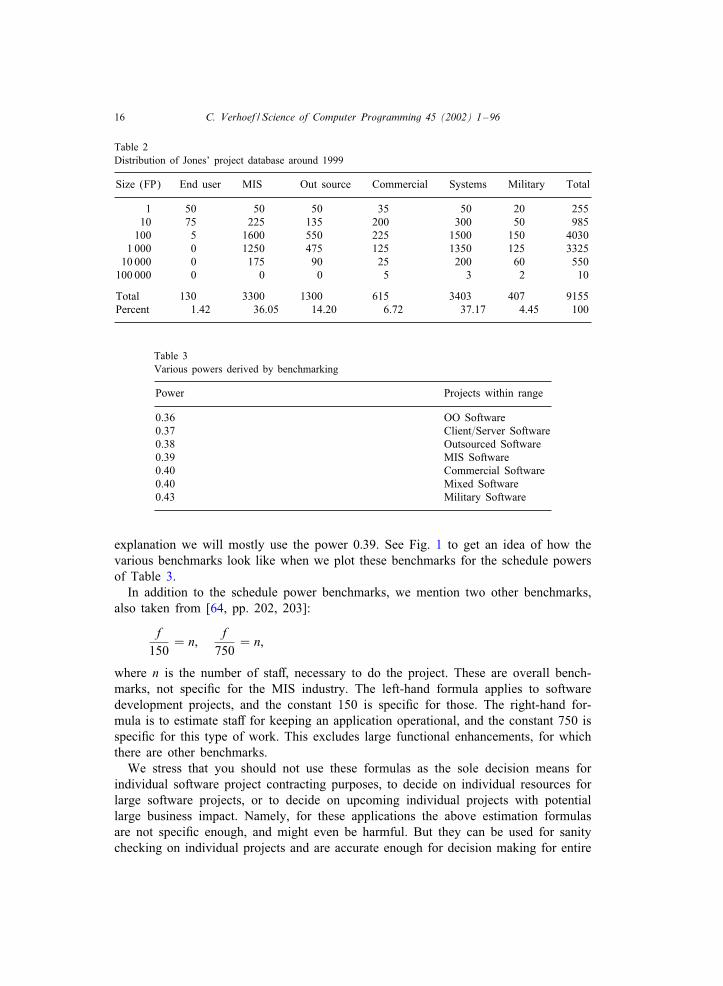
How much belief should we have in such a benchmark? There is no establishedtradition in software benchmarking and therefore the amount of projects subject tobenchmarking is relatively low. For instance, the latest benchmark release of the ISBSG(International Software Benchmarking Standards Group) is based on the 789 projectsthat were submitted to their repository in early 2000. We base our work mostly onJones’ database who has probably the largest knowledge base on software projects inthe world: in 1996 it contained 6753 projects [62, p. 161]. In 1999 this has grownto more than 9000 projects. We provide the distribution of the projects over sizeand type in Table 2. The database contains data regarding software comprising over10 million function points. To compare, a large international bank approximately owns450 000 function points of software, and a large life insurance company possesses550 000 function points [62, p. 51]. Jones partitioned his project database also overage range, partitioned it into new, enhancement, and maintenance projects, partitionedit over selected programming languages, and over a number of technologies used;see [62, pp. 162–164] for details. The overall set of projects used in producing thebenchmarks is biased: the database contains presumably more large projects than inreality [62, pp. 159–160]. But a CMM level 1 organization has no historical data toderive its own internal benchmarks, so we resort to Jones’ work as a surrogate forlack of historical information. Note that the schedule powers vary for diOerent codesizes, and for diOerent industries. We give you a few of such benchmarked powersthat you can use depending on the industry you are in, or depending on the type ofproject. Table 3 contains a few of them and is taken from [64, pp. 202]. For ease of
16 C. Verhoef / Science of Computer Programming 45 (2002) 1–96
Table 2Distribution of Jones’ project database around 1999
Size (FP) End user MIS Out source Commercial Systems Military Total
1 50 50 50 35 50 20 25510 75 225 135 200 300 50 985
100 5 1600 550 225 1500 150 40301 000 0 1250 475 125 1350 125 3325
10 000 0 175 90 25 200 60 550100 000 0 0 0 5 3 2 10
Total 130 3300 1300 615 3403 407 9155Percent 1.42 36.05 14.20 6.72 37.17 4.45 100
Table 3Various powers derived by benchmarking
Power Projects within range
0.36 OO Software0.37 Client=Server Software0.38 Outsourced Software0.39 MIS Software0.40 Commercial Software0.40 Mixed Software0.43 Military Software
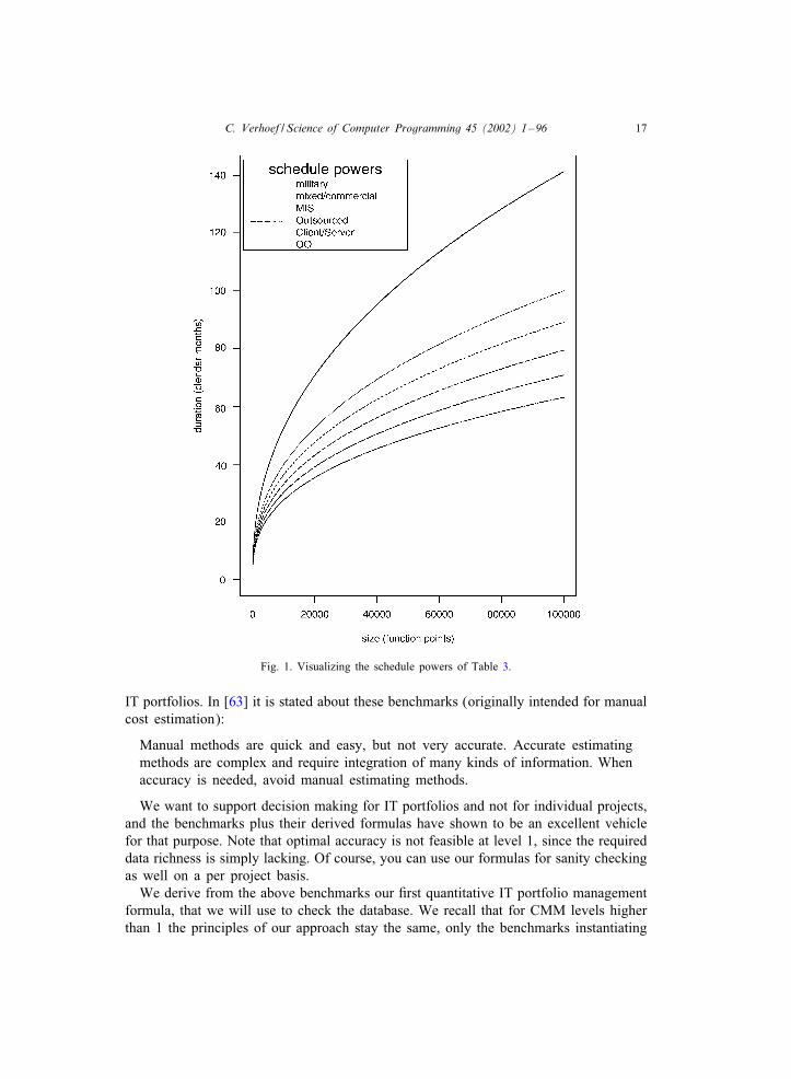
explanation we will mostly use the power 0:39. See Fig. 1 to get an idea of how thevarious benchmarks look like when we plot these benchmarks for the schedule powersof Table 3.
In addition to the schedule power benchmarks, we mention two other benchmarks,also taken from [64, pp. 202, 203]:
f150
= n;f
750= n;
where n is the number of staO, necessary to do the project. These are overall bench-marks, not speciCc for the MIS industry. The left-hand formula applies to softwaredevelopment projects, and the constant 150 is speciCc for those. The right-hand for-mula is to estimate staO for keeping an application operational, and the constant 750 isspeciCc for this type of work. This excludes large functional enhancements, for whichthere are other benchmarks.
We stress that you should not use these formulas as the sole decision means forindividual software project contracting purposes, to decide on individual resources forlarge software projects, or to decide on upcoming individual projects with potentiallarge business impact. Namely, for these applications the above estimation formulasare not speciCc enough, and might even be harmful. But they can be used for sanitychecking on individual projects and are accurate enough for decision making for entire
C. Verhoef / Science of Computer Programming 45 (2002) 1–96 17
Fig. 1. Visualizing the schedule powers of Table 3.
IT portfolios. In [63] it is stated about these benchmarks (originally intended for manualcost estimation):
Manual methods are quick and easy, but not very accurate. Accurate estimatingmethods are complex and require integration of many kinds of information. Whenaccuracy is needed, avoid manual estimating methods.
We want to support decision making for IT portfolios and not for individual projects,and the benchmarks plus their derived formulas have shown to be an excellent vehiclefor that purpose. Note that optimal accuracy is not feasible at level 1, since the requireddata richness is simply lacking. Of course, you can use our formulas for sanity checkingas well on a per project basis.
We derive from the above benchmarks our Crst quantitative IT portfolio managementformula, that we will use to check the database. We recall that for CMM levels higherthan 1 the principles of our approach stay the same, only the benchmarks instantiating
18 C. Verhoef / Science of Computer Programming 45 (2002) 1–96
our formulas change. Since there is more and better data available, it becomes feasibleto infer company-speciCc benchmarks, leading to more accurate instantiations of ourCrst formula. We discuss the instantiation using public benchmarks so that level 1organizations can use it.
We show a simple algebraic derivation to illustrate how you can derive your owninstantiation of our Crst formula in case you want to apply our results. First calculatehow many function points the application is according to benchmark.
f = d1
0:39 = d2:564:
We made f explicit using elementary algebraic arithmetic. With the second bench-mark, we calculate the number of people for the development project:
n =1
150d2:564:
So, the total number of calendar months m needed to accomplish the project ism=d · n. This amounts to
m =d
150d2:564:
We assume that there are w working days in a year, and for a given daily burdenedcompensation rate r we can now calculate the total cost of development tcd(d) for agiven project duration d:
tcd(d) = r · w12
· d150
· d2:564 =rwd1800
· d2:564 =rw
1800· d3:564
So the Crst formula for quantitative IT portfolio management is
tcd(d) =rw
1800· d3:564: (1)
Completely analogously, we derived a formula calculating the total cost of a main-tenance project for a given duration d (for costs to keep a system operational you donot know the duration per se, and we will derive other formulas for that, see formula11). For this second one we used the 750 benchmark for maintenance staO size, every-thing else being equal. Formula (2) for quantitative IT portfolio management thenbecomes
tcm(d) =rw
9000· d3:564: (2)
Of course the rates will vary per organization but also per task: we have used dailyrates ranging from 500 to 4000 US dollar. Certain programmers for ERP packagescan be more expensive, but also experts in high performance transaction processing atlarge banks and in the airline industry can be quite expensive (think of TPF experts[55]). We experienced that daily burdened compensation rates for both internal staOand external specialists were always available. Also the number of working days varies
C. Verhoef / Science of Computer Programming 45 (2002) 1–96 19
per organization and per country and can range from less than 200 to 230+ days peryear. You have to use your own company-speciCc rates to instantiate formulas (1) and(2) for quantitative IT portfolio management.
If you only know the total cost of an IT project, you can calculate the projectduration according to benchmark. We can do this with the dual versions of the Crst andsecond formulas. Without bothering you with the details of their (mathematically trivial)inference, we formulate formulas (3) and (4) for quantitative IT portfolio management:
dd(c) =(
1800cwr
)0:28
; (3)
md(c) =(
9000cwr
)0:28
; (4)
where dd is development duration, md is maintenance duration and c is the knowntotal cost of either a development or a maintenance project.
We also experienced that actual staO size is sometimes available in a number ofbusiness units. It is very useful to collect this information as well in the IT portfoliodatabase. Formulas (5) and (6) provide you with a benchmarked relation between staOsize and project duration:
nsd(d) =d2:564
150; (5)
nsm(d) =d2:564
750: (6)
where nsd is the number of staO for development, and nsm is the number of staO formaintenance projects. With formulas (5) and (6) you can detect diOerences betweenactual staO size and benchmarked staO size. In the same way, you can detect diOerencesbetween actual cost and benchmarked cost. Likewise, we can calculate for a givenstaO size the benchmarked duration, leading to formulas (7) and (8) for quantitativeIT portfolio management (QIPM):
dd(n) = (150n)0:39; (7)
md(n) = (750n)0:39; (8)
where n is the actual staO size, dd is development duration, and md is maintenanceduration.
We already made some example calculations, and we will make some more examplecalculations to illustrate the use of these formulas to support quantitative IT portfoliomanagement. Throughout the paper we assume for all example calculations a Cctiouscompany with a daily burdened rate of $1000 both for development, maintenance,internal and externally, and 200 working days per year. This leads to the following
20 C. Verhoef / Science of Computer Programming 45 (2002) 1–96
instantiations of formulas (1)–(4) for QIPM:
tcd(d) =1000
9· d3:564;
tcm(d) =2009
· d3:564;
dd(c) =(
9c1000
)0:28
;
md(c) =(
9c200
)0:28
:
For example, a 36 month development project costs tcd(36) = $39:1 million accord-ing to benchmark, and an 18 month maintenance project costs according to benchmarktcm(18) = $0:66 million. We announced earlier that when you know the costs, youcan calculate the duration. For a $5M development project dd(5M) = 20 indicatingthat such a project should take about 20 months. The number of staO nsd(20) = 15leading to 300 calendar months, or 25 man-year, which is indeed $5M. Likewise, a$5M maintenance project, takes md(5M) = 31:5 calendar months according to bench-mark and takes nsm(31:5) = 9:3 maintenance staO. This is 293 calendar months, leadingto $4.9 million, which accurately approximates the actual Cnancials.
4.1. Cleaning the IT portfolio database
Using formulas (1)–(8) you can check and clean your just compiled IT portfoliodatabase, by carrying out the process outlined below. Note that the goal is not tocomply with our formulas as closely as possible—the goal is to spot the diOerencesso you can locate and correct erroneous IT portfolio database entries after which thereal deviations according to benchmarked management information are revealed. Thesedeviations need the attention of the IT portfolio manager or IPM, which can be theCIO, a board member, or someone directly reporting to the executive board.
• Calculate the project durations from available data such as start and end dates.• Complete the portfolio database with lacking project durations, or Cnancials of all
projects beyond some threshold. Depending on the size of the company this thresholdis higher or lower. For large organizations we experienced that 5 million dollar is anacceptable threshold. For our Cctious organization this means that when reported costsof development or maintenance exceed $5M, the actual project duration needs to berecovered by inspecting the documents, or if all else fails asking the responsible ITmanager. Likewise this implies that for dd($5M) = 20 calendar month developmentprojects and md($5M) = 31 calendar month maintenance eOorts, the actual data needsto be recovered. We use the following simple guidelines for that:
◦ between $5 and 10 million, contact the system owner and just ask for the lackingactuals;
◦ between $10 and 25 million, in addition to asking for actuals also ask for the fulldocumentation of the IT project;
C. Verhoef / Science of Computer Programming 45 (2002) 1–96 21
◦ for IT investments exceeding $25M, lacking any other management information(which is not unusual in level 1 organizations), additionally do a function pointanalysis.
If instead of costs, management information comprises duration or staO size, useone of our other formulas to calculate the appropriate thresholds. For instance, usingformula (3) we calculate that dd($5M) = 20, and dd($10M) = 24, so the Crst projectduration threshold for our Cctious company is between 20 and 24 months. The othersare inferred similarly.
• Calculate only development costs according to benchmark for all projects (usingformula (1)). Mostly, IT projects that just keep applications running are combinedwith projects that add functionality to the business. In the less common case that pure(corrective) maintenance projects are separately reported, you will see a deviationwith the formula (1). Then you can correct for this by using formula (2).
• Compare the benchmarked costs with the actual Cnancials in the database and recordobvious deviations.
• Assess the deviations, and correct errors in the database if that was the cause. Welist a few common causes: project costs can be erroneously converted from localcurrencies to the chosen currency for the database, no conversion was done, no onecould Cnd the Euro sign so the local currency sign is used, with the undocumentedassumption that it should be read as Euro amounts. We also encountered the wrongnumber of zeros, decimal commas in the wrong location, and so on. Also erro-neous date information is a common cause for errors. For instance, the initiation anddelivery dates are exchanged, or a typo in the year is made leading to a huge diOer-ence, but also date formats are not uniform. For a globally operating organization,we experienced that the following issue was a common cause of errors: the date02=03=04 means in Japan the 4 March 2002, in the USA it stands for the 3 ofFebruary 2004, while in other parts of the world the 2 of March 2004 is implied.
• Assess the remaining deviations. First look at projects that are much too low com-pared to the actuals. They may be corrective maintenance projects. Separate out theseprojects and use formula (2) to carry out the process we are describing.
• When the Cnancials are much higher than expected, inspect the available projectdata. It can be that large hardware costs are incorporated in the IT project’s budget,then correct for them. It can also be the case that an expensive software packageor tool is acquired for this project. Think of ERP implementations. Then correct forthe package costs, and check whether the daily compensation rate is suJcient, sinceERP specialists can be much more expensive than other programmers. Then separateout these projects and use an ERP instantiation of formula (1) with the appropriatefully loaded daily compensation rate.
• When the Cnancials are much lower than expected, it may be the case that thisproject was outsourced to a cheap labor country. Inspect the available project datato correct for several things: Crst of all the power should be altered from 0:39 to0:38 in accordance with Table 3 for outsourced software. Also check for the numberof working days per annum in the country of outsourcing, and Cnally correct for
22 C. Verhoef / Science of Computer Programming 45 (2002) 1–96
the daily compensation rate. Use the oO-shore outsourcing variant of formula (1) fordevelopment projects, and a variant of formula (2) for operations projects for theseitems in the IT portfolio database.
• It can also be the case that projects under the same name are clustered. This can bea cluster of simultaneous projects. Typically, you will get a very high total cost fora much too short time frame. Then the projects need to be separated out, and theirdurations listed separately. You cannot simply add project durations, since there isno linear relation between duration and cost. Or in an equation:
tcd(d1 + d2) �= tcd(d1) + tcd(d2):
For example take a cluster of two projects, with d1 = 12 and d2 = 5. They separatelycost tcd(12) = $0:77 resp. tcd(5) = $0:03 million, so in total $0.80 million. But ad1 + d2 = 17 month project leads to tcd(17) = $2:69 million, so more than 3 timesthe total of the two projects.
• You also see entries where the project duration is very long but the costs are verylow. Then often people accumulated several related projects into one, and added thevarious project durations, e.g., the start and Cnish dates of a Gantt chart [38,104]comprising all subprojects. Also these projects should get separate entries plus thetime spent for each project in the cluster. Like above, you cannot add costs becauseof the nonlinearity of the relation, or in an equation:
dd(c1 + c2) �= dd(c1) + dd(c2):
For example, two subprojects costing c1 = 1 and c2 = 2 million dollar, respectively,will have a duration of dd($1M) = 12:7 and dd($2M) = 15:5 months each accordingto benchmark. While a c1+c2 = 3 million dollar project takes dd($3M) = 17:4 monthsaccording to benchmark. However, the combined subprojects take 28.3 months, whichwould incur a cost of tcd(28:3) = 16:7 million dollar according to benchmark.
• If the deviations can no longer be clariCed by errors, inaccuracies, linear thinking,or special project characteristics, the error correction process is Cnished. This doesnot mean that the contents is correct. It just means that most of the errors are gone,which is good enough for starting quantitative IT portfolio management.
• Calculate all instances of formulas (1) and (2), containing the appropriate rates andnumber of working days per year, for all projects.
The above process leads in a relatively short time to a reasonably accurate IT port-folio database. Now we are ready to analyze its contents.
5. Analyzing an IT portfolio database
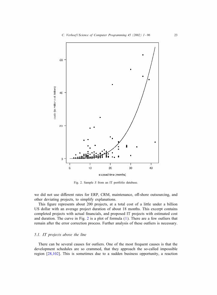
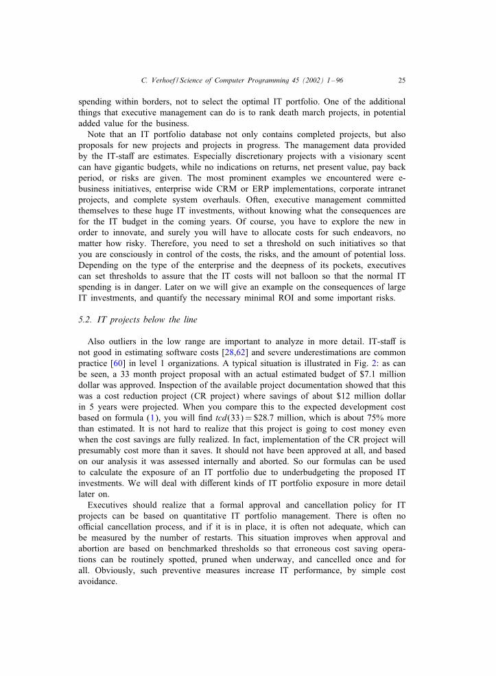
In Fig. 2 we composed a random excerpt of several IT portfolio databases fromorganizations that went through the above process—let’s call this sample S for laterreference. We changed daily compensation rates and variations in working days per yearto the example rates: a $1000 daily rate, and 200 working days per annum. Moreover,
C. Verhoef / Science of Computer Programming 45 (2002) 1–96 23
Fig. 2. Sample S from an IT portfolio database.
we did not use diOerent rates for ERP, CRM, maintenance, oO-shore outsourcing, andother deviating projects, to simplify explanations.
This Cgure represents about 200 projects, at a total cost of a little under a billionUS dollar with an average project duration of about 18 months. This excerpt containscompleted projects with actual Cnancials, and proposed IT projects with estimated costand duration. The curve in Fig. 2 is a plot of formula (1). There are a few outliers thatremain after the error correction process. Further analysis of these outliers is necessary.
5.1. IT projects above the line
There can be several causes for outliers. One of the most frequent causes is that thedevelopment schedules are so crammed, that they approach the so-called impossibleregion [28,102]. This is sometimes due to a sudden business opportunity, a reaction
24 C. Verhoef / Science of Computer Programming 45 (2002) 1–96
on a competitor that demands a full focus on speed to market, but can also be dueto lack of governance by executive management. Whatever the reason: such projectshave a high price tag, are risky, and too many of them can decrease IT performanceconsiderably, leading to value destruction. The project costs and failure risks drama-tically increase when the development schedule is compressed to the impossible region.Plotting formula (1) against the development projects in an IT portfolio gives you aquick overview of the outliers, that are probably death march projects [136]. For theseprojects you can analyze whether the need for speed was really that urgent, and ifso, whether the incurred initial costs plus the high risk of failure justiCed the projectsby a sureCre business opportunity. For, when the costs balloon due to this type ofdevelopment, the returns should be obvious, the pay back period should be relativelyshort, and performance should be measurable.
You will also run into high-risk low-reward projects in the portfolio: death marchprojects where the hurry is not justiCed by the potential returns. The two outliersaround the 20 million dollar and the one of 25 million dollar were non-discretionaryprojects. Executive management does not consider these projects as strategic, since theymust be done irrespective the strategy. But you can do them the smart and the stupidway. Usually, non-discretionary projects are initiated too late and therefore exposethe enterprise to high costs and unnecessary risks. Better governance of these non-discretionary projects leads to better IT performance, by cost avoidance.
So also non-discretionary projects need timely executive attention. Especially, whenthey potentially aOect large parts of the organization. Some frequent examples of unnec-essary costly non-discretionary projects that we spotted in various IT portfolio studiesare: operating system updates, platform migrations, Y2K projects, Euro conversions,programming language or dialect conversions, conversions to 10-digit bank accountnumbers (as required by the European Central Bank), and more. The nature of thesenon-discretionary projects is not special in the sense that they are of an extremelyexpensive nature, but they become unnecessarily costly by negligence. Non-discretionaryprojects should not be high-risk no-reward projects destroying value, but sometimesthey are. For instance, Y2K costs consumed up to 30% of the total IT budgets in1999 [125, p. 30]. For non-discretionary projects careful timely planning utilizing asmuch as automation is key, so that costs are brought to the absolute minimum. Totalcosts decrease when the schedules are relaxed, that is, when the projects are plannedwell-ahead of the deadline [102]. Moreover, the projects are done more rapidly andaccurately when automated tools are used. Gartner Group advised to use so-called soft-ware renovation factories [130] when the code volume exceeds a few million lines ofcode [50,66] for Y2K updates. This advise remains valid for other modiCcations thatpotentially impact large parts of single systems or an unknown number of systems inan entire IT portfolio.
Apart from these unnecessary costs, there will always be death march projects thatcan be justiCed by proper business reasons. Executive management should consciouslydecide on acceptable risks, and put a threshold on death march projects for an ITportfolio. We recall that for this kind of analysis modern portfolio theory [79] is notadequate: you cannot abandon information technology like junking bonds. You haveto live with a lot of suboptimal IT. Setting this threshold is just a way to keep the IT
C. Verhoef / Science of Computer Programming 45 (2002) 1–96 25
spending within borders, not to select the optimal IT portfolio. One of the additionalthings that executive management can do is to rank death march projects, in potentialadded value for the business.
Note that an IT portfolio database not only contains completed projects, but alsoproposals for new projects and projects in progress. The management data providedby the IT-staO are estimates. Especially discretionary projects with a visionary scentcan have gigantic budgets, while no indications on returns, net present value, pay backperiod, or risks are given. The most prominent examples we encountered were e-business initiatives, enterprise wide CRM or ERP implementations, corporate intranetprojects, and complete system overhauls. Often, executive management committedthemselves to these huge IT investments, without knowing what the consequences arefor the IT budget in the coming years. Of course, you have to explore the new inorder to innovate, and surely you will have to allocate costs for such endeavors, nomatter how risky. Therefore, you need to set a threshold on such initiatives so thatyou are consciously in control of the costs, the risks, and the amount of potential loss.Depending on the type of the enterprise and the deepness of its pockets, executivescan set thresholds to assure that the IT costs will not balloon so that the normal ITspending is in danger. Later on we will give an example on the consequences of largeIT investments, and quantify the necessary minimal ROI and some important risks.
5.2. IT projects below the line
Also outliers in the low range are important to analyze in more detail. IT-staO isnot good in estimating software costs [28,62] and severe underestimations are commonpractice [60] in level 1 organizations. A typical situation is illustrated in Fig. 2: as canbe seen, a 33 month project proposal with an actual estimated budget of $7.1 milliondollar was approved. Inspection of the available project documentation showed that thiswas a cost reduction project (CR project) where savings of about $12 million dollarin 5 years were projected. When you compare this to the expected development costbased on formula (1), you will Cnd tcd(33) = $28:7 million, which is about 75% morethan estimated. It is not hard to realize that this project is going to cost money evenwhen the cost savings are fully realized. In fact, implementation of the CR project willpresumably cost more than it saves. It should not have been approved at all, and basedon our analysis it was assessed internally and aborted. So our formulas can be usedto calculate the exposure of an IT portfolio due to underbudgeting the proposed ITinvestments. We will deal with diOerent kinds of IT portfolio exposure in more detaillater on.
Executives should realize that a formal approval and cancellation policy for ITprojects can be based on quantitative IT portfolio management. There is often nooJcial cancellation process, and if it is in place, it is often not adequate, which canbe measured by the number of restarts. This situation improves when approval andabortion are based on benchmarked thresholds so that erroneous cost saving opera-tions can be routinely spotted, pruned when underway, and cancelled once and forall. Obviously, such preventive measures increase IT performance, by simple costavoidance.
26 C. Verhoef / Science of Computer Programming 45 (2002) 1–96
5.3. Synonyms, homonyms, redundancies
As soon as you compile an IT portfolio database, you will Cnd multiple occurrencesof the same project under a diOerent name (synonyms) and multiple occurrences of thesame name but describing diOerent projects (homonyms). Synonyms can be removedfrom the database, and homonyms should be renamed so that you can diOerentiatebetween them.
In addition you will Cnd existing and proposed systems that are redundant. Recallthat in CIO Magazine, it is reported that just compiling an IT portfolio database savedone company $3 million and another company $4.5 million because the IT portfolioview enabled them to spot redundancies [5]. While we spotted redundancies as well,and could prevent unnecessary spending at times, you have to be careful with beingtoo enthusiastic with removal of redundancies. There are two types of redundancies:similar proposed systems and similar existing systems.
First we deal with proposals. An often seen eOect after an IT portfolio is compiled,is that similar proposals are put together and carried out as one combined joint project.Only if all the envisioned systems are going to be exactly the same it is likely toreap beneCts from removing redundancies, by cancelling one but all the proposals.If another approach is taken towards redundancy, this leads to an increase in stake-holders, increase in necessary Iexibility, more variation points, increased organizationalcomplexity, multiple ownership adding to the complexity, increased feature creep, anda larger size of the new system. Larger size implies, more time to develop, more risk.Let us make a calculation to illustrate the possible consequences of removing seemingredundancies. Suppose you Cnd two 12 month projects that are fairly similar. Usingformula (1), each project will cost $780 000 according to benchmark. So two of them,cost $1.56 million. Using formula (3) we can calculate what the development timeis of a single $1.56 million project. This is 14.5 months. It is highly unlikely thatthe variation points, the increased number of stakeholders, and the other issues justmentioned will be solved in 2.5 months. So the synergy that looks good on managementcharts is very unlikely to be accomplished. Moreover this synergistic strategy easilyleads to a grand IT project. Something that is strongly discouraged in the ClingerCohen act [45], since this is known not to be working out properly. We quote:
Reduce risk and enhance manageability by discouraging “grand” informationsystem projects, and encouraging incremental, phased approaches.
Now let us have a look at existing systems that seem redundant at Crst sight. Whilethis can be extremely frustrating, it is not uncommon that an organization has multiplesimilar systems. You cannot get rid of them without signiCcant investments, if at all.For instance, the US Department of Defense owns more than 700 payroll systems, overa 100 personnel training systems, and myriads of intranets [121]. How easy it is toremove such redundancies is also illustrated by the failure of GTE Corporation (then aleading telecommunications provider) to consolidate an overall medicare system. TheUS Secretary of Health and Human Services announced in 1994 that: “We’re going tomove from the era of the quill pen to the era of the superelectronic highway”. Thisto provide timely payment, and reduce fraudulent claims. GTE spent $100 million
C. Verhoef / Science of Computer Programming 45 (2002) 1–96 27
for a uniCed medicare system and learned that they had to integrate many separateinformation systems. In 1997 the project was cancelled. According to GTE this projectwas far more complicated than anyone anticipated.
Solving this kind of problem is much more involved than removing redundant auto-mobiles, buildings, or other tangible assets. The problem is that these systems look likeredundancies from the executive viewpoint, but are more like homonyms. There aremultiple variation points, and to consolidate those into one overall system takes sophis-ticated software engineering technology. You have to migrate the similar systems to asoftware product line [32]. CMM level 1 organizations are most likely not equipped toinitiate, migrate, and deploy such complex software artifacts. Apart from that, redun-dancy in IT is not necessarily a bad thing. In [32] we call this the relativistic e<ectsof software engineering, meaning that the classical way of thinking about softwarebreaks down when the size increases, just like Newton’s laws of physics break downwhen speed increases. For small systems, and small user communities redundancy canbe avoided entirely. But as soon as variation points are necessary, the ideal situationis that changes only important for one user should not aOect another user. If redun-dancy is weeded out completely, inevitably, users will have to accept new releases ofthe software also when the modiCcation was not meant for them. The release eOortfor the business will then be higher than the cost of dealing with redundancy at thedevelopment site. See [32] for quantitative data supporting our arguments in detail. Soredundancy is not necessarily a bad thing, and focusing on its removal should not bethe prime task of an IPM.
While many business assets can be truly redundant, this is hardly ever the case forIT. In article [5] where the cost savings for redundancy are reported on, it is statedthat IT is not special, that it operates like any other part of business. With the abovearguments we have illustrated that IT is special. Apart from our arguments, the specialstatus of IT has been subject to discussion for decades. For provocative enlightment,we refer to a classical paper we mentioned earlier: the note by Lamport [73] explainingthat maintaining software is entirely diOerent from maintaining an automobile.
6. The black hole: hidden costs
Apart from the high costs of death march projects, high-risk visionary projects, andother costly eOorts, there are also hidden costs that you need to be aware of. Let uscontinue with the CR project example to illustrate what we mean by this. Apart fromthe fact that the total development costs of the underbudgeted CR project are in theorder of $30 million according to benchmark, there will also be an additional minimalcost of operation during the entire deployment phase of this system, excluding separateenhancement projects. But how to quantify such costs? In this section we develop moreformulas to calculate this according to benchmark. For instance, we can calculate withthese formulas that for the coming 5 years the costs to keep the CR project operationalare benchmarked at $10.4 million. This alone almost annihilates the projected costreduction of $12 million in 5 years. Moreover there will be more operational costsif the system is not retired after 5 years of deployment. The minimal total cost of
28 C. Verhoef / Science of Computer Programming 45 (2002) 1–96
ownership is around $48.3 million according to benchmark, so even when the costsavings over the Crst 5 years will more than double over the rest of the deploymentphase, to say $30 million, there is a net loss of in the order of $20 million over theentire lifetime of the system. So, even when the project was estimated correctly, theoperational costs are high, and are prolonging the pay back period signiCcantly, makingthe entire investment questionable.
It is our experience that the above calculations are not made when assessing ITproposals. However, they show that IT investments can easily lead to proCt destructioninstead of the expected value creation, not only by underbudgeting but also by nottaking the operational costs over time into account. The accumulation of operationalcosts of IT projects plus the existence of proCt destructing IT projects that were notanticipated is giving many executives the feeling that IT is a black hole. This feeling issupported by facts. Many large companies suOer from high operational and maintenancecosts, 60% and more of the total IT budget is no exception. The US average in 1994was that about 45% of the total budget was spent on maintenance [60]. This impliesthat almost half the annual IT budget was spent on operations and maintenance. Thesecosts are increasing, given the fact that more and more IT personnel is working inmaintenance [63,64]. These alarming Cgures are beginning to attract the attention ofcorporate management. The Cndings are no freak accidents, but have been reportedover and over again for decades [34,8,26,77,106,6,51,63,102,81]. In those publicationspercentages between 50 and 80% devoted to maintenance costs are reported.
Also the cost per unit of work diOers for development and deployment work onsoftware. Already in the seventies this was empirically found. In [127] a ratio of1:50 is reported, and in one US Air Force study Barry Boehm found that the costper instruction was $30 while the cost per instruction for maintenance was $4000—a ratio of 1:133 [7]. For executives it is not clear what maintainers do, since thesoftware was running in the Crst place to their understanding. Therefore, to obtaincontrol over your IT portfolio it is crucial to know about these hidden costs. Onlythen it becomes possible to control your IT budget for the existing portfolio, and toproject the operational costs for future systems that are proposed to be added to yourIT portfolio. We will develop formulas that take operational costs into account.
6.1. Minimal total cost of ownership
Of course, it is hard to predict maintenance eOort, since a lot of maintenance isnot just keeping software running. It is more than that: enhancement to align systemsbetter with new business needs. Those costs are often in your IT portfolio database,and are denoted as development projects (on existing systems). There are howeversubstantial costs connected to the operational phase of software systems that are oftennot described in IT projects and therefore do not end up in your IT portfolio. Forthose hidden costs we will develop more formulas supporting quantitative IT portfoliomanagement. Using the formulas it becomes much more clear what the real thresholdsfor ROI should be (we come back to this later on). In eOect, we need to compare thepotential value creation with the potential total cost of ownership in order to deciderationally on IT investments.
C. Verhoef / Science of Computer Programming 45 (2002) 1–96 29
To be able to say something about total cost of ownership, we need to know howlong the software will be operational. With the Y2K problem we have seen that thiscan be much longer than expected. Or as Strassmann put it [122, p. 253]:
Software is a new form of immortality.
In level 1 organizations where no measurement history is in place, there is also nolifetime data available, so we need to compensate for this lack of information by usinga public benchmark taken from [60, p. 419]:
f1=4 = y;
where y is the number of calendar years the software will be deployed (f stands forfunction points again). From this benchmark, and the benchmark for MIS software(f0:39 =d), we can immediately derive two new QIPM formulas (9) and (10):
y(d) = d0:641; (9)
d(y) = y1:56: (10)
Note that for other industries, you have to adapt the schedule power using Table 3.For example, for a 34 month MIS development project we can calculate that accordingto benchmark this software will be deployed y(34) = 9:6 years, we used this formulain the previous section to see whether the cost reduction project would really savecosts.
Formula (10), which is the dual of formula (9) can be used to estimate how mucheOort is reasonable for projects of which you know how long the software will benecessary. For instance, a company needed a conversion tool to automatically con-vert Cobol 85 back to an older dialect Cobol 74 [15] for the coming 37 months atmost. This is a systems software project, and because of the implementation methodsthat are going to be used, it is acceptable to use the power for OO software (0:36in Table 3). So, then the instantiation of formula (10) for the power 0:36 leads to:d(y) =y1:44. Its development time should not be longer than d(37=12) = 5:1 months.We use the OO schedule power to instantiate formula (1) for this project, leading to:tcd(d) = rw=1800 ·d3:7778. We keep r = $1000, and w= 200 days. We calculate thattcd(5:1) = 50 800 dollar to develop the tool seems reasonable, given the limited timeyou need the tool in the Crst place. If the costs are deviating considerably, it is timeto assess the price setting of the tool supplier.
With formula (9) we can derive another formula that for a given project duration dmeasured in calendar months, gives us the minimal costs to keep the developed systemoperational. We will show later on that this is indeed a lower bound, so the actualcosts could be higher, but presumably not lower than our formula calculates. We areinterested in estimating the minimal cost of operation during the entire deploymenttime of a software system, based on the development time of the IT project. This isin fact:
mco(d) = y(d) · wr · nsm(d):
30 C. Verhoef / Science of Computer Programming 45 (2002) 1–96
For, in one calendar year, you work w days at daily compensation rate r, withnsm(d) people, for y(d) calendar years. Combining formulas (9) and (6) then leadsto formulas (11) and (12):
mco(d) =wr750
· d3:205; (11)
dd(o) =(
750wr
· o)0:312
: (12)
Again, dd stands for development duration. We used formula (11) for the earliermentioned 33 month CR project: indeed the minimal cost of operation mco(33) = 19:6M$, the deployment phase is according to formula (9): y(33) = 9:4 years, so after 5years, $10.4M operational cost turns the estimated $12 million savings into $0.8 whichis easily annihilated by the 75% underestimated cost of development.
Formula (12) is useful for rough estimates for merging, acquisition, and outsourcing.Let us give an example of the latter. You can use formula (12) as an indicator whetheroutsourced operational costs make sense at all. Often you know the total contractualoperational costs o for a number of years to keep a system operational. Suppose thereis a contract with an outsourcer to keep a system running for $10 million a year forthe coming 10 years. Then, using formula (12), we can calculate that the developmenttime of this project was probably dd($100M) = 54:8 calendar months. And this impliesthat the deployment phase is approximately y(54:8) = 13 years. So depending on theactual development time (that could be present in your IT portfolio database) you canget an impression whether the outsourcer is too expensive, or if the software is reallythat large, you may want to rethink the contract to prolong it. The latter also dependson the added value for the business. The same type of calculation can be done whenyou want to acquire a company and you know total operational costs. Of course, thisis an indicative estimate.
We can derive from formulas (1) and (11) the minimal total cost of ownership.Formula (13) supporting QIPM is
mtco(d) = tcd(d) + mco(d): (13)
So, for a given project duration you can calculate the minimal total cost of ownershipmtco(d) of a system over the entire life cycle according to benchmark.
Let us give an example to show that the above formula makes sense. Suppose there isa project proposal that takes 36 calendar months. Total cost of development accordingto benchmark is tcd(36) = 39:1 million dollar. The minimal cost of operation accordingto benchmark is mco(36) = 25:9 million dollar. So, minimal total cost of ownershipmtco(36) of this software system is 65.0 million dollar. The Crst three years 39.1 M$is spent, and the subsequent y(36) = 9:9 years, 25.9 $M=year is needed to keep itrunning. Indeed, 60.1% is spent on development, and 39.9% is needed to keep thesystem operational. Recall that our estimates use a minimal scenario: keep the systemsrunning without large enhancements. So, our Cndings converge with the empirical datathat are found for several decades [34,8,26,77,106,6,51,63,102,81].
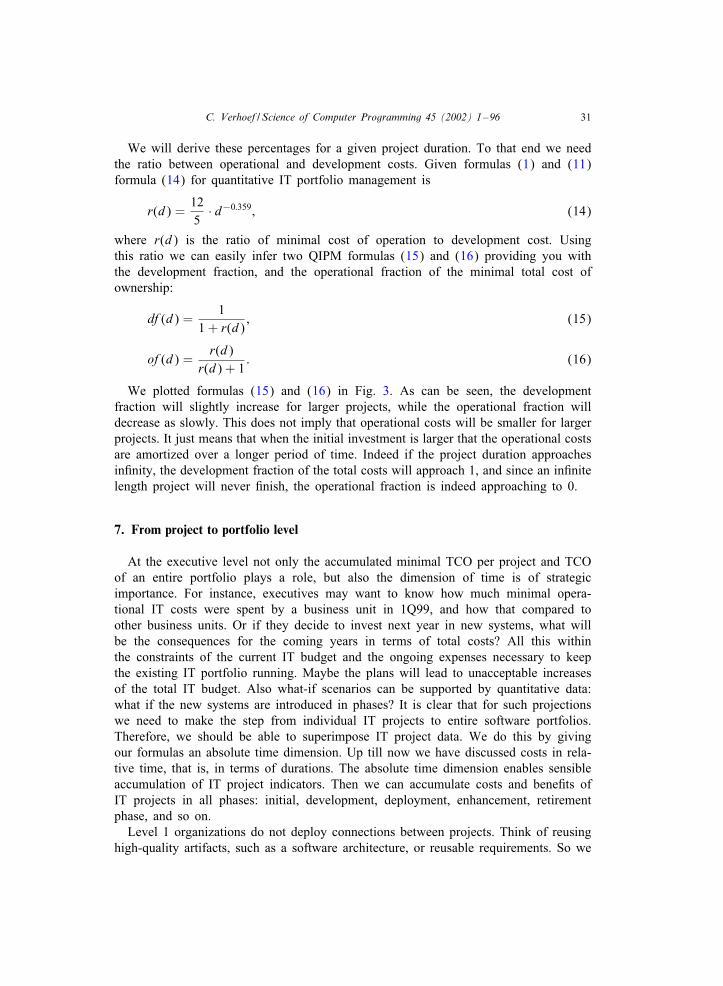
C. Verhoef / Science of Computer Programming 45 (2002) 1–96 31
We will derive these percentages for a given project duration. To that end we needthe ratio between operational and development costs. Given formulas (1) and (11)formula (14) for quantitative IT portfolio management is
r(d) =125
· d−0:359; (14)
where r(d) is the ratio of minimal cost of operation to development cost. Usingthis ratio we can easily infer two QIPM formulas (15) and (16) providing you withthe development fraction, and the operational fraction of the minimal total cost ofownership:
df (d) =1
1 + r(d); (15)
of (d) =r(d)
r(d) + 1: (16)
We plotted formulas (15) and (16) in Fig. 3. As can be seen, the developmentfraction will slightly increase for larger projects, while the operational fraction willdecrease as slowly. This does not imply that operational costs will be smaller for largerprojects. It just means that when the initial investment is larger that the operational costsare amortized over a longer period of time. Indeed if the project duration approachesinCnity, the development fraction of the total costs will approach 1, and since an inCnitelength project will never Cnish, the operational fraction is indeed approaching to 0.
7. From project to portfolio level
At the executive level not only the accumulated minimal TCO per project and TCOof an entire portfolio plays a role, but also the dimension of time is of strategicimportance. For instance, executives may want to know how much minimal opera-tional IT costs were spent by a business unit in 1Q99, and how that compared toother business units. Or if they decide to invest next year in new systems, what willbe the consequences for the coming years in terms of total costs? All this withinthe constraints of the current IT budget and the ongoing expenses necessary to keepthe existing IT portfolio running. Maybe the plans will lead to unacceptable increasesof the total IT budget. Also what-if scenarios can be supported by quantitative data:what if the new systems are introduced in phases? It is clear that for such projectionswe need to make the step from individual IT projects to entire software portfolios.Therefore, we should be able to superimpose IT project data. We do this by givingour formulas an absolute time dimension. Up till now we have discussed costs in rela-tive time, that is, in terms of durations. The absolute time dimension enables sensibleaccumulation of IT project indicators. Then we can accumulate costs and beneCts ofIT projects in all phases: initial, development, deployment, enhancement, retirementphase, and so on.
Level 1 organizations do not deploy connections between projects. Think of reusinghigh-quality artifacts, such as a software architecture, or reusable requirements. So we
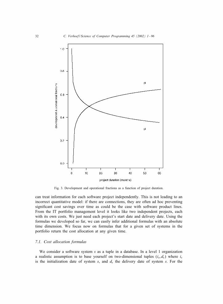
32 C. Verhoef / Science of Computer Programming 45 (2002) 1–96
Fig. 3. Development and operational fractions as a function of project duration.
can treat information for each software project independently. This is not leading to anincorrect quantitative model: if there are connections, they are often ad hoc preventingsigniCcant cost savings over time as could be the case with software product lines.From the IT portfolio management level it looks like two independent projects, eachwith its own costs. We just need each project’s start date and delivery date. Using theformulas we developed so far, we can easily infer additional formulas with an absolutetime dimension. We focus now on formulas that for a given set of systems in theportfolio return the cost allocation at any given time.
7.1. Cost allocation formulas
We consider a software system s as a tuple in a database. In a level 1 organizationa realistic assumption is to base yourself on two-dimensional tuples (is; ds) where isis the initialization date of system s, and ds the delivery date of system s. For the
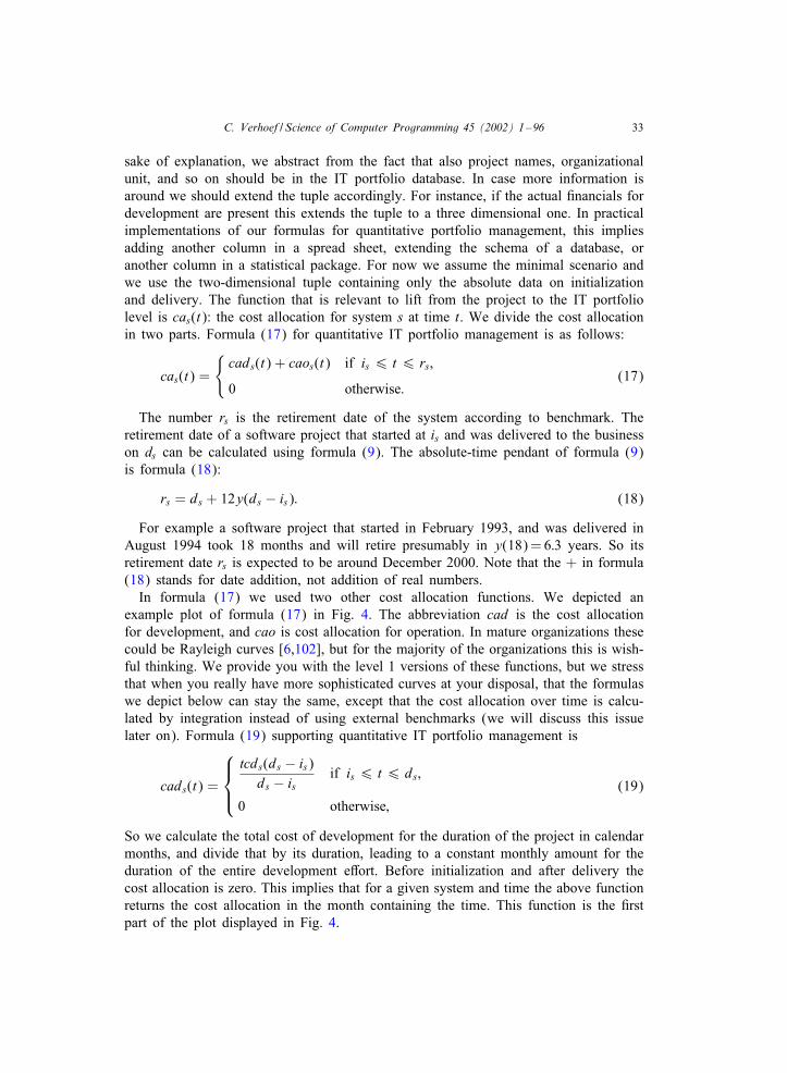
C. Verhoef / Science of Computer Programming 45 (2002) 1–96 33
sake of explanation, we abstract from the fact that also project names, organizationalunit, and so on should be in the IT portfolio database. In case more information isaround we should extend the tuple accordingly. For instance, if the actual Cnancials fordevelopment are present this extends the tuple to a three dimensional one. In practicalimplementations of our formulas for quantitative portfolio management, this impliesadding another column in a spread sheet, extending the schema of a database, oranother column in a statistical package. For now we assume the minimal scenario andwe use the two-dimensional tuple containing only the absolute data on initializationand delivery. The function that is relevant to lift from the project to the IT portfoliolevel is cas(t): the cost allocation for system s at time t. We divide the cost allocationin two parts. Formula (17) for quantitative IT portfolio management is as follows:
cas(t) =
{cads(t) + caos(t) if is 6 t 6 rs;
0 otherwise:(17)
The number rs is the retirement date of the system according to benchmark. Theretirement date of a software project that started at is and was delivered to the businesson ds can be calculated using formula (9). The absolute-time pendant of formula (9)is formula (18):
rs = ds + 12y(ds − is): (18)
For example a software project that started in February 1993, and was delivered inAugust 1994 took 18 months and will retire presumably in y(18) = 6:3 years. So itsretirement date rs is expected to be around December 2000. Note that the + in formula(18) stands for date addition, not addition of real numbers.
In formula (17) we used two other cost allocation functions. We depicted anexample plot of formula (17) in Fig. 4. The abbreviation cad is the cost allocationfor development, and cao is cost allocation for operation. In mature organizations thesecould be Rayleigh curves [6,102], but for the majority of the organizations this is wish-ful thinking. We provide you with the level 1 versions of these functions, but we stressthat when you really have more sophisticated curves at your disposal, that the formulaswe depict below can stay the same, except that the cost allocation over time is calcu-lated by integration instead of using external benchmarks (we will discuss this issuelater on). Formula (19) supporting quantitative IT portfolio management is
cads(t) =
tcds(ds − is)ds − is
if is 6 t 6 ds;
0 otherwise;(19)
So we calculate the total cost of development for the duration of the project in calendarmonths, and divide that by its duration, leading to a constant monthly amount for theduration of the entire development eOort. Before initialization and after delivery thecost allocation is zero. This implies that for a given system and time the above functionreturns the cost allocation in the month containing the time. This function is the Crstpart of the plot displayed in Fig. 4.
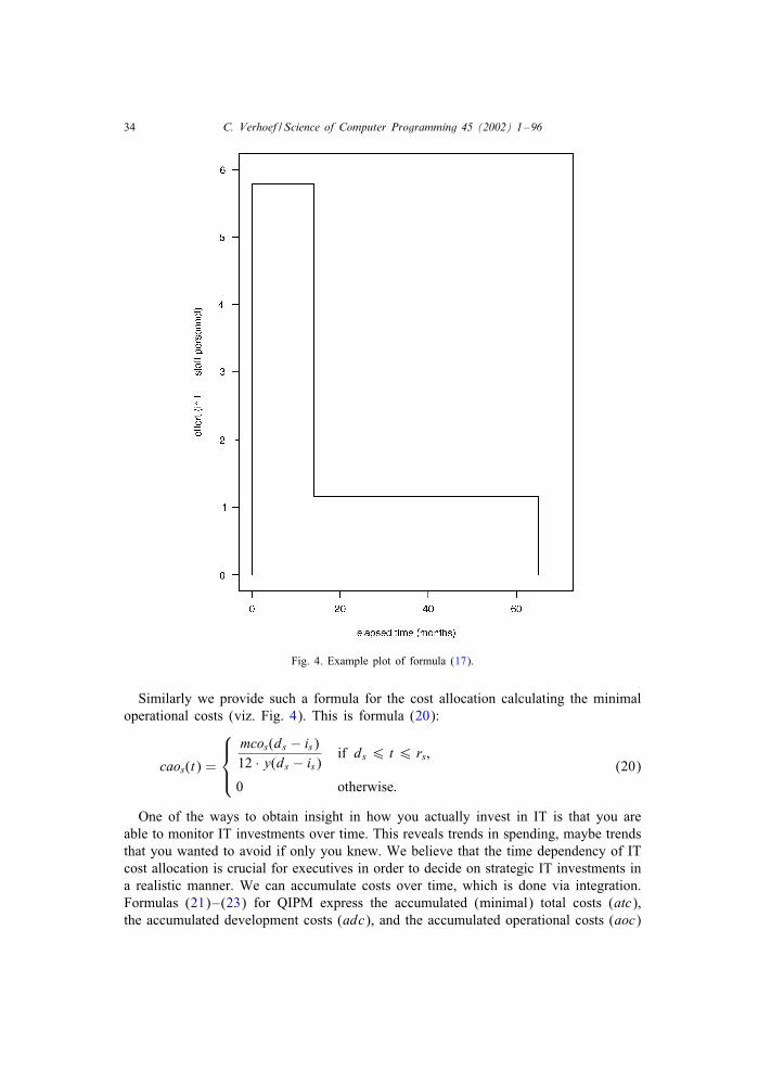
34 C. Verhoef / Science of Computer Programming 45 (2002) 1–96
Fig. 4. Example plot of formula (17).
Similarly we provide such a formula for the cost allocation calculating the minimaloperational costs (viz. Fig. 4). This is formula (20):
caos(t) =
mcos(ds − is)12 · y(ds − is)
if ds 6 t 6 rs;
0 otherwise:(20)
One of the ways to obtain insight in how you actually invest in IT is that you areable to monitor IT investments over time. This reveals trends in spending, maybe trendsthat you wanted to avoid if only you knew. We believe that the time dependency of ITcost allocation is crucial for executives in order to decide on strategic IT investments ina realistic manner. We can accumulate costs over time, which is done via integration.Formulas (21)–(23) for QIPM express the accumulated (minimal) total costs (atc),the accumulated development costs (adc), and the accumulated operational costs (aoc)

C. Verhoef / Science of Computer Programming 45 (2002) 1–96 35
over a given time interval T for a certain software system s.
atcs(T ) =∫
t∈Tcas(t) dt; (21)
adcs(T ) =∫
t∈Tcads(t) dt; (22)
aocs(T ) =∫
t∈Tcaos(t) dt; (23)
where cas, cads, and caos are cost allocation functions. They can be the ones that wedeCned in formulas (17), (19) and (20), but they can also be more sophisticated formu-las, like Rayleigh curves, or more sophisticated curves (we explain them later on). Nowwe can go from the project level to the portfolio level. This is done via summation,since there are only Cnitely many systems in a portfolio. For a given portfolio P anda given time interval T we can calculate accumulated (minimal) total costs for a port-folio, the accumulated development costs for a portfolio, and accumulated operationalcosts for a portfolio. Formulas (24)–(26) are:
atcP(T ) =∑s∈P
atcs(T ); (24)
adcP(T ) =∑s∈P
adcs(T ); (25)
aocP(T ) =∑s∈P
aocs(T ): (26)
We can use these formulas to answer the questions like the ones we posed earlier.How to compare operational costs of say 5 business units in the Crst quarter of 1999?For Cve business units BU1; : : : ;BU5 you can calculate the total minimal operationalIT cost for 1Q99 using the following simple formula:
∑s∈BUi
∫t∈1Q99
caos(t) dt; i = 1; : : : ; 5:
We assume that for these business units we have their systems in the IT portfoliodatabase, and that we have initialization and delivery dates of the projects. With thisdata, we can calculate for each system the operational cost allocations for the Crstquarter of 1999, and accumulate these Cgures for all the systems in the portfolio of aspeciCc business unit. In this way you can compare operational cost per business unitand zoom in on diOerences, signaling trends that may need attention. For instance, ifbusiness unit 1 is now at CMM level 2, does this lead to lower operational costs?And if so, is it more than the costs of obtaining CMM level 2 and maintaining thatlevel? And if so, how much could we save if we would do this for other business unitsas well? Note that it is not at all obvious whether operational costs will go down incase of better approaches to develop systems. The costs tend to become higher [27],
36 C. Verhoef / Science of Computer Programming 45 (2002) 1–96
this is not too much of a problem if the systems create value. It can also be the casethat one business unit is consuming the majority of the total operational budget in thecorporate IT portfolio. Depending on the criticality and proCtability of such a businessunit, corporate executives can decide on diOerent strategies: phasing out, selling, orreengineering and so on.
7.2. Hitting the innovation borders
Already in the early 1990s some fortune 500 companies found themselves trapped inthe situation where their entire IT budget was gobbled up with updating, repairing andenhancing their aging legacy applications [60]. This does not need to be a dangeroussituation if you reached exactly that level of automation that you wanted. But it is morelikely that when you are in such a situation, you are exposed to unacceptable businessrisks. The environment changes fast and unpredictably, so to stay competitive, youhave to innovate. This means that you must have the supporting budget. But since allnew development adds to the operational pressure, you cannot innovate without limits.So, you need to keep track of how much of the IT budget is spent on operational costsat all times to know in advance whether operational costs start to hinder the amount ofinnovation that executive management deems appropriate for the company. This impliesthat to initiate new development you probably Crst need to retire existing systems,reduce operational costs, or increase the total IT budget. The minimal operational costsare signiCcant as we already indicated with formula (11). We will now derive whatthis means in terms of absolute time.
We calculate the ratio between operational costs and development costs per unitof time. If you have sophisticated data available you can calculate this using actualvalues, but in level 1 organizations this information is usually absent. So we use ourcost allocation formulas to calculate this ratio. Note that we in fact calculate the ratiobetween the heights of both rectangulars in Fig. 4. The height of the Crst rectangular is
tcds(ds − is)ds − is
and the height of the second rectangular is
mcos(ds − is)12y(ds − is)
:
Division yields
mcos(ds − is)tcds(ds − is)
· ds − is12(ds − is)0:641 =
125
· (ds − is)−0:359
12(ds − is)0:359
=15;
using formula (14) for the relative ratio, and formula (9). This results in the Cxed ratioequation (27):
caos : cads = 5 : 1: (27)
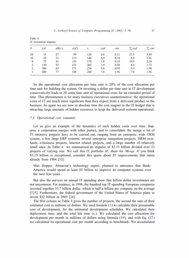
C. Verhoef / Science of Computer Programming 45 (2002) 1–96 37
Table 4IT investment impulse
# tcd dd(c) y(d) rs cad cao∑
cad∑
cao
50 15 27 99 126 0.6 0.11 27.5 5.4910 30 33 113 146 0.9 0.18 9.0 1.816 75 43 133 176 1.8 0.35 10.5 2.103 150 52 151 203 2.9 0.58 8.6 1.732 300 63 171 234 4.8 0.95 9.5 1.901 600 77 188 260 7.8 1.56 7.8 1.56
So the operational cost allocation per time unit is 20% of the cost allocation pertime unit for building the system. Or investing a dollar per time unit in IT developmentconservatively leads to 20 cents=time unit of operational costs for an extended period oftime. This phenomenon is for many business executives counterintuitive: the operationalcosts of IT are much more signiCcant than they expect from a delivered product to thebusiness. So again we see now in absolute time the cost magnet in the IT budget that isattracting large amounts of hidden resources to keep the delivered systems operational.
7.3. Operational cost tsunamis
Let us give an example of the dynamics of such hidden costs over time. Sup-pose a corporation merges with other parties, and to consolidate the merge a lot ofIT intensive projects have to be carried out, ranging from an enterprise wide CRMsystem, a few large ERP systems, several enterprise integration projects, HRM over-hauls, e-business projects, Internet related projects, and a large number of relativelysmall ones. In Table 4 we summarized an impulse of $3.15 billion divided over 72projects of varying size. We call this IT portfolio M , short for Merge. If you think$3.15 billion is exceptional, consider this quote about IT improvements that stemsalready from 1984 [53]:
Max Hopper, Armacost’s technology expert, planned to announce that Bank-America would spend at least $5 billion to improve its computer systems overthe next few years.
But also the surveys on annual IT spending show that billion dollar investments arenot uncommon. For instance, in 1998, the hundred top IT-spending European companiesinvested together 53.7 billion dollar, which is half a billion per company on the average[125]. Furthermore, the federal government of the United States of America plans toinvest $52 billion in 2003 [24].
The Crst column in Table 4 gives the number of projects, the second the sum of theirestimated cost in millions of dollars. We used formula (3) to calculate their presumablecost of development, for the estimated development schedules. We calculated theirdeployment time, and the total life time (rs). We calculated the cost allocation fordevelopment per month in millions of dollars using formula (19), and with Eq. (27)we calculated its operational cost per month according to benchmark. We accumulated
38 C. Verhoef / Science of Computer Programming 45 (2002) 1–96
Table 5Accumulation of cost allocation data
Development Operations
Time Cost Time Cost Time Cost
27 72.9 27 5.49 127 14.633 45.4 33 7.3 146 9.143 36.4 43 9.4 176 7.152 25.9 52 11.1 203 5.263 17.3 63 13.0 234 3.577 7.8 77 14.6 271 1.6
these costs for all projects leading to the last 2 columns. We supposed that all 72projects start shortly after the merge. Some of them are outsourced, others are doneinternally, the IT workforce is extended with myriads of people, and so on. It is nothard to calculate the accumulated costs for the entire portfolio for development andoperations in absolute time as summarized in Table 5.
We visualized these data points in Fig. 5. As you can see there is a signiCcant costimpulse in the Crst 25 months that rapidly declines after about 50 months.
Next, we use the accumulated data to derive the cost allocation function for ITportfolio M . The accumulated cost allocation function for development is the peakyone. We use standard parametric statistical techniques to infer a smooth curve fromthese data. Using an implementation of a nonlinear least squares regression algorithm[19,54,129,95] as implemented in the statistical system SPlus [129,72] the data pointscan be Ctted to the following curve:
cadM (t) = 7:514287t1:258007e−0:07304098t :
Recall that M is the IT portfolio consisting of the 72 projects in Table 4. Before wecontinue, a few words on the large amount of digits in the above formula. The datahas a certain precision, of course, but we try to Ct this data as good as possible, whichleads to the large amounts of digits. If we would round the above digits, an entirelydiOerent curve would show up. This is partly due to the exponential functions: a slightchange in its power is a huge change in the behavior of the curve. So we keep thesevery precise, so that we will not deviate from the input data. Second, the outcomesof using the formulas, are subject to the standard rounding rules. However, we willuse high precision outcomes so that readers who redo the calculations can convincethemselves that they made the right calculation. Of course, in practical applications youhave to round output of such formulas in accordance with the precision of the inputdata (but not the used coeJcients in those formulas).
The other curve represents operational costs. It is a curve with a long wave lengthand a 100 month lasting cost plateau. This plateau starts right after the IT investmentimpulse is over. Also the accumulated operational cost allocation function can be Cttedto a curve:
caoM (t) = 0:02643959t1:692713e−0:003407055t1:317413:
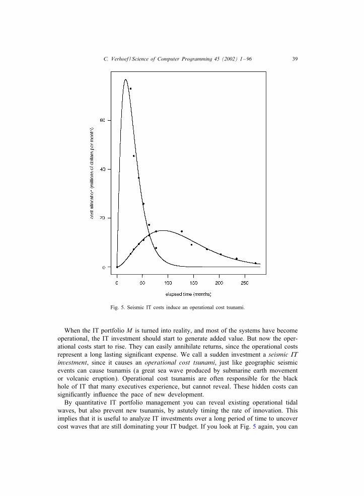
C. Verhoef / Science of Computer Programming 45 (2002) 1–96 39
Fig. 5. Seismic IT costs induce an operational cost tsunami.
When the IT portfolio M is turned into reality, and most of the systems have becomeoperational, the IT investment should start to generate added value. But now the oper-ational costs start to rise. They can easily annihilate returns, since the operational costsrepresent a long lasting signiCcant expense. We call a sudden investment a seismic ITinvestment, since it causes an operational cost tsunami, just like geographic seismicevents can cause tsunamis (a great sea wave produced by submarine earth movementor volcanic eruption). Operational cost tsunamis are often responsible for the blackhole of IT that many executives experience, but cannot reveal. These hidden costs cansigniCcantly inIuence the pace of new development.
By quantitative IT portfolio management you can reveal existing operational tidalwaves, but also prevent new tsunamis, by astutely timing the rate of innovation. Thisimplies that it is useful to analyze IT investments over a long period of time to uncovercost waves that are still dominating your IT budget. If you look at Fig. 5 again, you can
40 C. Verhoef / Science of Computer Programming 45 (2002) 1–96
see that many years after implementation of the $3.15 billion IT portfolio, signiCcantoperational costs of the seismic IT investment are still inIuencing the IT costs of thebusiness unit owning the portfolio.
With the accumulated cost allocation functions we have a potentially powerfulweapon to forecast future costs. First we calculate the accumulated development costfunction for the entire portfolio. We use formulas (25) and (22) for that:
adcM (T ) =∑s∈M
adcs(T ) =∑s∈M
∫t∈T
cads(t) dt
=∫
t∈T
∑s∈M
cads(t) dt =∫
t∈TcadM (t) dt
=∫
t∈T7:514287t1:258007e−0:07304098t dt:
We take the interval T = [0; t]:
adcM (T ) =∫ t
07:514287t1:258007e−0:07304098t dt
= 7:514287(419:087 − 368:192�(2:258007; 0:07304098t)):
You can use a computer algebra system like Maple [135] or Mathematica [132] forthis evaluation (but we used formula (39) that we discuss later on). The function �is a special mathematical function called the upper incomplete gamma function. Thisfunction satisCes the following equation:
�(a; x) =∫ ∞
xta−1e−t dt:
The accumulated development cost function approximates the total IT investmentaccurately: if we take T = [0;∞) we should get the total development budget of theportfolio back. Indeed, limx→∞ �(a; x) = 0, so
adcM (0;∞) = 7:514287 · 419:087 = 3149:14
million dollars. This outcome has a 0.02% diOerence with the actual investment of$3.15 billion. For the total minimal cost of operation we cannot do such a “regressiontest”, since those costs were never envisioned in the Crst place. But let’s calculate theaccumulated operational cost for M as well. We used formula (39) that we discusslater on, but you can also use a computer algebra system like Mathematica [132] orMaple [135] for this.
aocM (0; t) =∫ t
00:02643959t1:692713e−0:003407055t1:317413
dt
= 2262:23 − 2219:22�(2:043939903; 0:003407055t1:317413);
C. Verhoef / Science of Computer Programming 45 (2002) 1–96 41
so now we can see the total impact of operational costs for this portfolio over theentire life cycle of the portfolio. We Cnd aocM (0;∞) = 2262:23 million dollar. Thetotal cost of ownership of this portfolio thus amounts to 5411.37 million dollar. So,58.2% of the costs are devoted to development, and 41.8% is necessary for operations,which is in accord with the many empirical Cndings we quoted earlier. Note that thisIT investment impulse is now $2.3 billion short. Not all this money needs to be presentfrom the start, but should become available sometime in the future.
When does this future start? When the initial IT investment is fully consumed byimplementing it. We can calculate when this is the case. We know that the accumulatedtotal cost allocation for M is as follows:
atcM (0; t) = adcM (0; t) + aocM (0; t)
= 5411:37
− 2219:22�(2:043939903; 0:003407055t1:317413)
− 2766:70�(2:258007; 0:07304098t):
We calculated this formula simply by adding the above two derived formulas. Weplot the three accumulated cost functions in Fig. 6. This is an insightful graph givingyou an indication of the probable spending situation over the forthcoming years. Wecan already see that somewhere between month 50 and 60 the money will probably runout. We use this rough estimate as an initial value for root Cnding. With the computeralgebra system Mathematica [132] we solved the root of the following equation (butwe could have used Maple [135] or Matlab [80] as well):
atcM (0; t) − 3150 = 0;
yielding t = 57:3123 months. So, the money runs out after 57 months. After that timestamp we really need a positive return from the IT investment to subsidize the missing2:3 billion. Not immediately, but in due time. When these returns should becomeavailable is our next subject.
7.4. ROI threshold quavering
After about 50 months, most of the systems in the example IT portfolio have becomeoperational, that is, when atcM (50) = $2900 million is spent. The next hundred months,we need another
atcM (150) − atcM (50) = 1838:87
million dollar, to Cnalize development and keep the portfolio running. Suppose thatthe investment plan for our example IT portfolio projected an annual return of 10%,starting after 50 months (which is more than 4 years), then in the Crst year after these50 months the portfolio should add a value of 315 million. However, you have to
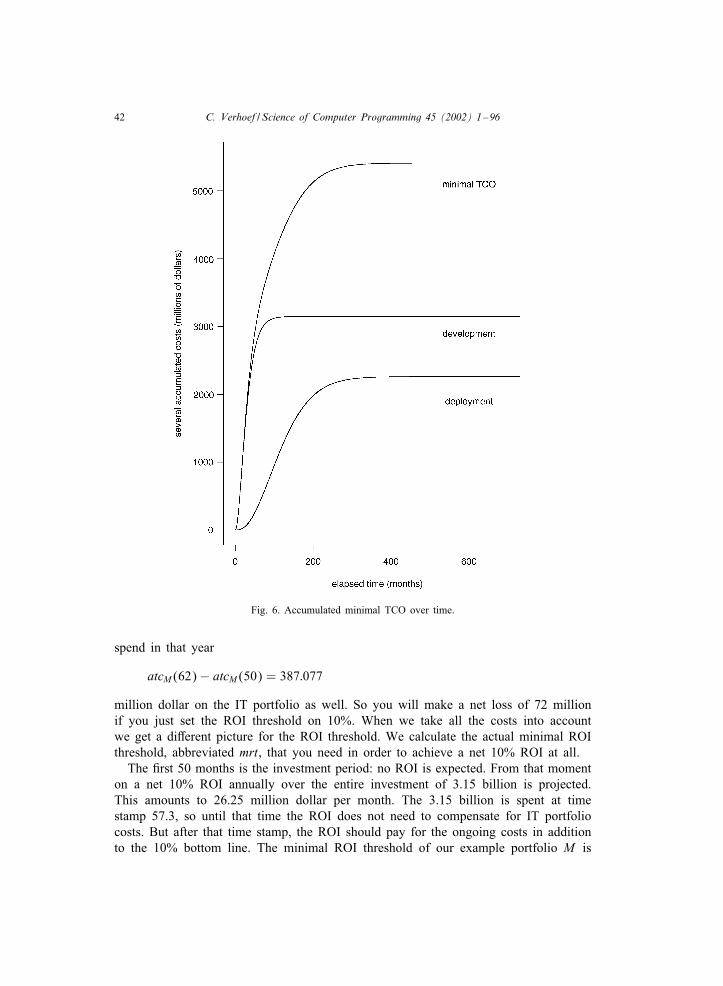
42 C. Verhoef / Science of Computer Programming 45 (2002) 1–96
Fig. 6. Accumulated minimal TCO over time.
spend in that year
atcM (62) − atcM (50) = 387:077
million dollar on the IT portfolio as well. So you will make a net loss of 72 millionif you just set the ROI threshold on 10%. When we take all the costs into accountwe get a diOerent picture for the ROI threshold. We calculate the actual minimal ROIthreshold, abbreviated mrt, that you need in order to achieve a net 10% ROI at all.
The Crst 50 months is the investment period: no ROI is expected. From that momenton a net 10% ROI annually over the entire investment of 3.15 billion is projected.This amounts to 26.25 million dollar per month. The 3.15 billion is spent at timestamp 57.3, so until that time the ROI does not need to compensate for IT portfoliocosts. But after that time stamp, the ROI should pay for the ongoing costs in additionto the 10% bottom line. The minimal ROI threshold of our example portfolio M is
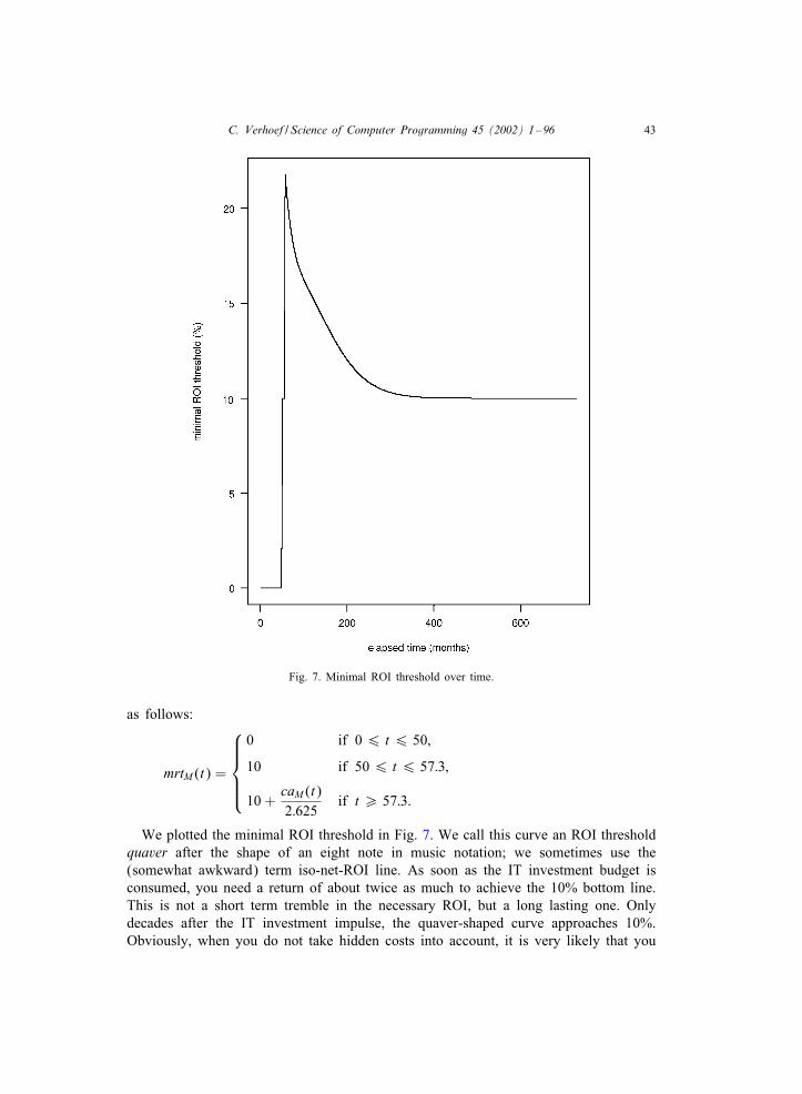
C. Verhoef / Science of Computer Programming 45 (2002) 1–96 43
Fig. 7. Minimal ROI threshold over time.
as follows:
mrtM (t) =
0 if 0 6 t 6 50;
10 if 50 6 t 6 57:3;
10 +caM (t)2:625
if t ¿ 57:3:
We plotted the minimal ROI threshold in Fig. 7. We call this curve an ROI thresholdquaver after the shape of an eight note in music notation; we sometimes use the(somewhat awkward) term iso-net-ROI line. As soon as the IT investment budget isconsumed, you need a return of about twice as much to achieve the 10% bottom line.This is not a short term tremble in the necessary ROI, but a long lasting one. Onlydecades after the IT investment impulse, the quaver-shaped curve approaches 10%.Obviously, when you do not take hidden costs into account, it is very likely that you
44 C. Verhoef / Science of Computer Programming 45 (2002) 1–96
will never have a positive return on investment, if the actual proCts of the IT investmentcannot compensate the ROI quaver.
8. IT portfolio exposure
Apart from the fact that IT spending is much more costly than many of usenvision and that projected returns are not always met (e.g., if ROI threshold qua-vering is not taken into account) there is also another dimension to quantitative ITportfolio management, that can seriously hinder achieving added value: IT risks. Mc-Farlan [82], proposed already in 1981 that risks of IT projects should be assessed notonly separately, but also in the aggregate—as a portfolio. While McFarlan proposed arisk assessment questionnaire, we quantify risk based on benchmark data. We believethat risk assessment will beneCt from a combination of quantitative and qualitativeinformation.
In the introduction we already indicated that the risks of software projects are high.As Standish group found, 50% is challenged, and 30% of the IT projects fail. But,can you project these numbers directly on your own IT portfolio? The answer isno. But executives need to get an indication of the ratios of successful, challengedand failed projects. Since there is no historical data on such topics in CMM level 1organizations, and understandably, this information is usually hidden for executives, weneed to compensate for this by using public benchmarks. In this section we show howyou can obtain an indication of the IT portfolio exposure based on project durations.This is not necessarily the ideal method to quantify risk, but usually it is the only wayfor level 1 organizations to get an indication at all.
Adding to the complexity of risks is that some executives think that you can justoverhaul IT systems, this is not true. However, it is not a surprise that people think likethis: our calculations with respect to IT portfolios revealed that even in the unlikelycase that your systems do not need enhancements, the costs to keep them operationalare huge. Moreover, enhancing these systems makes things worse: the costs increase.So it makes sense to ask yourself, why not renew these costly systems?
Once these often costly systems are up and running their failure exposure is lowerthan in a new situation, where childhood diseases, and infant mortality are notuncommon [58,46–48,42,41,44]. You could see a deployed system as a set of exe-cutable requirements needing continuous debugging, reCnement, and extension. Whilethis can be a frustrating task, cherishing existing business-critical systems is often pay-ing oO much more than overhauling these systems by new ones. Strassmann noticedthis as well, given that he writes [122, pp. 258, 257]:
For an enterprise with a large accumulation of legacy systems—which includes allestablished organizations—there are no technical strategies other than evolutionarymigration strategies. DeCning the path of such migration requires placing limitedobjectives along the way. The managerial skill in coming up with such a plan andthen making it happen will be the ultimate test which only superior informationmanagement teams will pass. [..] In the future, information political contests will
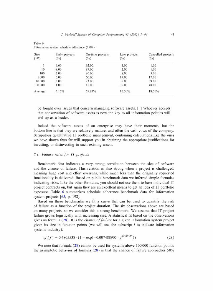
C. Verhoef / Science of Computer Programming 45 (2002) 1–96 45
Table 6Information system schedule adherence (1999)
Size Early projects On-time projects Late projects Cancelled projects(FP) (%) (%) (%) (%)
1 6.00 92.00 1.00 1.0010 8.00 89.00 2.00 1.00
100 7.00 80.00 8.00 5.001 000 6.00 60.00 17.00 17.00
10 000 3.00 23.00 35.00 39.00100 000 1.00 15.00 36.00 48.00
Average 5.17% 59.83% 16.50% 18.50%
be fought over issues that concern managing software assets. [..] Whoever acceptsthat conservation of software assets is now the key to all information politics willend up as a leader.
Indeed the software assets of an enterprise may have their moments, but thebottom line is that they are relatively mature, and often the cash cows of the company.Scrupulous quantitative IT portfolio management, containing calculations like the oneswe have shown thus far will support you in obtaining the appropriate justiCcations forinvesting, or disinvesting in such existing assets.
8.1. Failure rates for IT projects
Benchmark data indicates a very strong correlation between the size of softwareand the chance of failure. This relation is also strong when a project is challenged,meaning huge cost and eOort overruns, while much less than the originally requestedfunctionality is delivered. Based on public benchmark data we inferred simple formulasindicating risks. Like the other formulas, you should not use them to base individual ITproject contracts on, but again they are an excellent means to get an idea of IT portfolioexposure. Table 6 summarizes schedule adherence benchmark data for informationsystem projects [65, p. 192].
Based on these benchmarks we Ct a curve that can be used to quantify the riskof failure as a function of the project duration. The six observations above are basedon many projects, so we consider this a strong benchmark. We assume that IT projectfailure grows logistically with increasing size. A statistical Ct based on the observationsgives us formula (28). It is the chance of failure for a given information system projectgiven its size in function points (we will use the subscript i to indicate informationsystems industry):
cf i(f) = 0:4805538 · (1 − exp(−0:007488905 · f0:587375)) (28)
We note that formula (28) cannot be used for systems above 100 000 function points:the asymptotic behavior of formula (28) is that the chance of failure approaches 50%
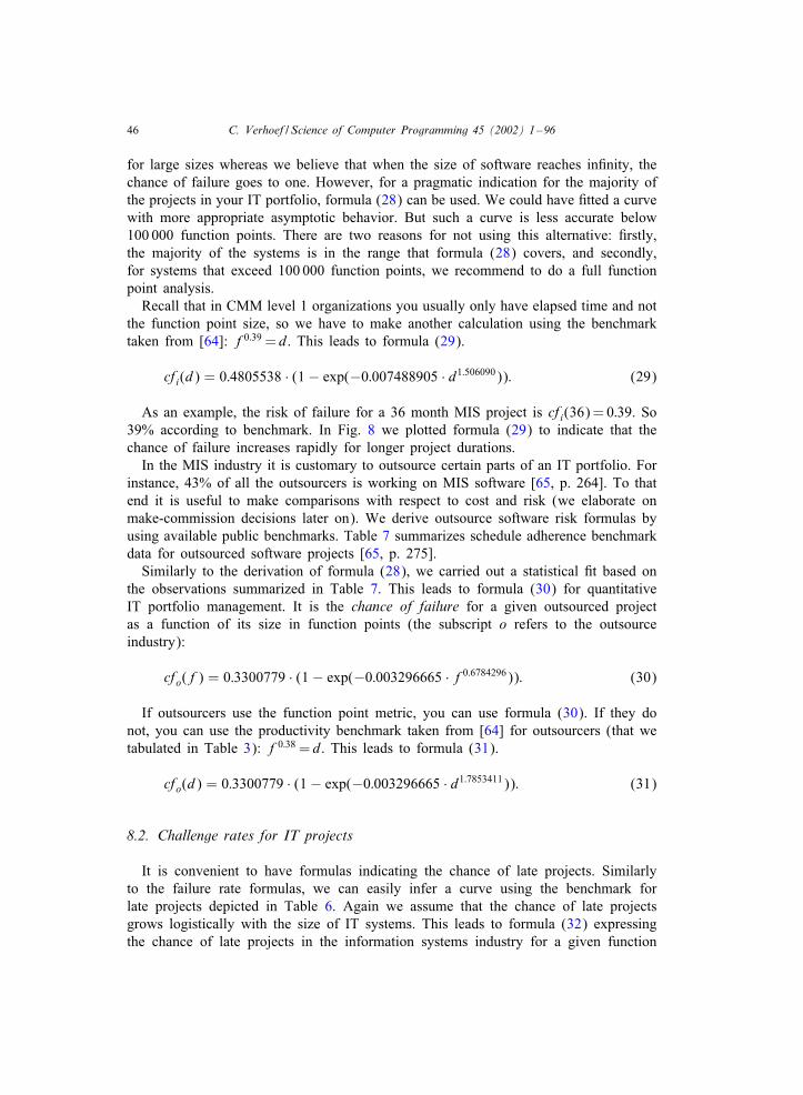
46 C. Verhoef / Science of Computer Programming 45 (2002) 1–96
for large sizes whereas we believe that when the size of software reaches inCnity, thechance of failure goes to one. However, for a pragmatic indication for the majority ofthe projects in your IT portfolio, formula (28) can be used. We could have Ctted a curvewith more appropriate asymptotic behavior. But such a curve is less accurate below100 000 function points. There are two reasons for not using this alternative: Crstly,the majority of the systems is in the range that formula (28) covers, and secondly,for systems that exceed 100 000 function points, we recommend to do a full functionpoint analysis.
Recall that in CMM level 1 organizations you usually only have elapsed time and notthe function point size, so we have to make another calculation using the benchmarktaken from [64]: f0:39 =d. This leads to formula (29).
cf i(d) = 0:4805538 · (1 − exp(−0:007488905 · d1:506090)): (29)
As an example, the risk of failure for a 36 month MIS project is cf i(36) = 0:39. So39% according to benchmark. In Fig. 8 we plotted formula (29) to indicate that thechance of failure increases rapidly for longer project durations.
In the MIS industry it is customary to outsource certain parts of an IT portfolio. Forinstance, 43% of all the outsourcers is working on MIS software [65, p. 264]. To thatend it is useful to make comparisons with respect to cost and risk (we elaborate onmake-commission decisions later on). We derive outsource software risk formulas byusing available public benchmarks. Table 7 summarizes schedule adherence benchmarkdata for outsourced software projects [65, p. 275].
Similarly to the derivation of formula (28), we carried out a statistical Ct based onthe observations summarized in Table 7. This leads to formula (30) for quantitativeIT portfolio management. It is the chance of failure for a given outsourced projectas a function of its size in function points (the subscript o refers to the outsourceindustry):
cfo(f) = 0:3300779 · (1 − exp(−0:003296665 · f0:6784296)): (30)
If outsourcers use the function point metric, you can use formula (30). If they donot, you can use the productivity benchmark taken from [64] for outsourcers (that wetabulated in Table 3): f0:38 =d. This leads to formula (31).
cfo(d) = 0:3300779 · (1 − exp(−0:003296665 · d1:7853411)): (31)
8.2. Challenge rates for IT projects
It is convenient to have formulas indicating the chance of late projects. Similarlyto the failure rate formulas, we can easily infer a curve using the benchmark forlate projects depicted in Table 6. Again we assume that the chance of late projectsgrows logistically with the size of IT systems. This leads to formula (32) expressingthe chance of late projects in the information systems industry for a given function
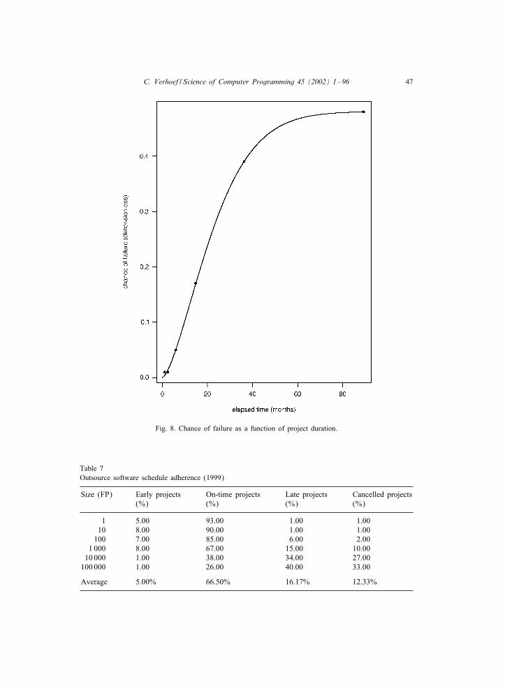
C. Verhoef / Science of Computer Programming 45 (2002) 1–96 47
Fig. 8. Chance of failure as a function of project duration.
Table 7Outsource software schedule adherence (1999)
Size (FP) Early projects On-time projects Late projects Cancelled projects(%) (%) (%) (%)
1 5.00 93.00 1.00 1.0010 8.00 90.00 1.00 1.00
100 7.00 85.00 6.00 2.001 000 8.00 67.00 15.00 10.00
10 000 1.00 38.00 34.00 27.00100 000 1.00 26.00 40.00 33.00
Average 5.00% 66.50% 16.17% 12.33%
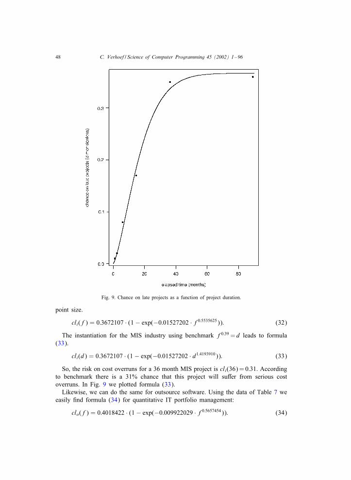
48 C. Verhoef / Science of Computer Programming 45 (2002) 1–96
Fig. 9. Chance on late projects as a function of project duration.
point size.
cl i(f) = 0:3672107 · (1 − exp(−0:01527202 · f0:5535625)): (32)
The instantiation for the MIS industry using benchmark f0:39 =d leads to formula(33).
cl i(d) = 0:3672107 · (1 − exp(−0:01527202 · d1:4193910)): (33)
So, the risk on cost overruns for a 36 month MIS project is cl i(36) = 0:31. Accordingto benchmark there is a 31% chance that this project will suOer from serious costoverruns. In Fig. 9 we plotted formula (33).
Likewise, we can do the same for outsource software. Using the data of Table 7 weeasily Cnd formula (34) for quantitative IT portfolio management:
clo(f) = 0:4018422 · (1 − exp(−0:009922029 · f0:5657454)): (34)
C. Verhoef / Science of Computer Programming 45 (2002) 1–96 49
If the outsourcers work with function points, you can use formula (34) immediately,and if not, you can use formula (35):
clo(d) = 0:4018422 · (1 − exp(−0:009922029 · d1:488804)): (35)
where we used the schedule power 0:38 as listed in Table 3.
8.3. Challenge and failure rates for portfolios
Knowing how to calculate prominent exposures on a per project basis, we can makethe step from individual projects to the portfolio level. We accumulate the projectexposures to obtain the portfolio exposure. You can then answer questions like: whichbusiness unit has the highest exposure to failed projects? For a given portfolio P thefailure exposure of P is formula (36):
fe(P) =1|P| ·
∑s∈P
cf (ds); (36)
where |P| is the number of systems in the portfolio, s is a system, ds is its projectduration, and cf is some derived chance of failure function, for instance formula (29)or (31). In this way you can calculate the average failure rate of the entire IT portfolio.It is up to executive management to set a threshold on the overall failure exposure ofan IT portfolio.
Similarly, for a given portfolio P the late exposure of P is formula (37):
le(P) =1|P| ·
∑s∈P
cl(ds) (37)
For instance, for the sample portfolio that we depicted in Fig. 2 we can calculateboth exposures: fe(S) = 0:13 and le(S) = 0:14. The sample portfolio has a chance offailure of 13%, and a 14% chance of serious cost overruns. For our seismic IT impulsedepicted in Table 4 we can likewise calculate that fe(M) = 0:126 and le(M) = 0:135.The percentages that Standish Group found, (30% cancelled, 50% challenged, 20%okay), are not found in many business unit level IT portfolios. This is due to the factthat per portfolio, only a fairly small number of very large projects are present. Atthe corporate level the percentages can be a bit higher, but still not approaching theStandish Group Cndings so closely, that you can use their benchmark to calculate yourIT portfolio exposures. This is due to the fact that large companies often have a lotof smaller business units. When only very large business units are present, also largerprojects are undertaken, with their risks. The Standish Group Cndings are accumulatedat the country level (for the USA). Maybe only the largest projects in the surveyedcompanies were taken into account.
Depending on the nature of the company and the deepness of its pockets, such ITportfolio exposures give you an indication whether you are within the exposure zonethat you consider acceptable. If not, it is time to mitigate those risks, and identify thecarriers of large exposures; they are almost always large IT projects (as McFarlan alsopointed out [82]).

50 C. Verhoef / Science of Computer Programming 45 (2002) 1–96
9. Comparison with higher CMM levels
A natural question is whether the accuracy of our approach explained so far willdrastically increase when the underlying mathematics is not based on level 1 formulas,but on formulas available to organizations with CMM levels that are higher than 1. Itis not easy to make comparisons, since there are hardly any published cost allocationcurves (which might be due to the fact that 75% of the organizations are at CMMlevel 1). Apart from that, many cost estimation techniques were traditionally based onlines of code, instead of function point-like metrics, such as the various versions offunction points [1,61], or Tom DeMarco’s bang metric [28]. It is known from thesoftware productivity literature that diOerent deCnitions for lines of code can leadto an uncertainty of 500%, rendering comparisons of diOerent estimates based onlines of code often useless [59, p. 16]. Recall that in [33, p. 132] even a 2300%variance was found for diOerent deCnitions for lines of code. Therefore, it is not asurprise that in a review article on software cost estimation techniques [84], huge dif-ferences were found when about 15 cost estimation techniques were applied to a singleproject.
Nevertheless we found an example curve in a textbook on software cost estimation.With this published example we illustrate that the results might not lead to radicallydiOerent decision making than in the level 1 situation. One argument why this is thecase, is that we are not using the actual relations between cost, eOort, and duration overtime, but rather their mean values, expressed by the area under cost allocation curves.If the areas are of the same order of magnitude, all calculations based on the areasunder these curves will be of the same order of magnitude as well, and therefore thedecision making will not drastically change. Of course, CMM level 2+ organizationshave historical data, which enables the derivation of internal benchmarks. They aremore precise than the external benchmarks that we use now. So the quality of thedecisions will improve, based on the input data that you can instantiate our formulaswith, but our method can still be used.
We give an example supporting the fact that more involved cost estimation formulasusually do not change the outcome of IT portfolio decision making. Note that ingeneral, it is a good idea to estimate software costs as accurately as possible.
In Boehm’s book on software engineering economics [6, p. 68] a Du BridgeChemical software development project is used as a running example. Its distributionis as follows.
ead(t) =mtp2 · exp−
(t2
2p2
):
The above function is called a Rayleigh curve; ead is the eOort allocation fordevelopment, m is again short for man-months, and p represents the month at whichthe project achieves its peak eOort. For the Du Bridge Chemical project, Boehm usedthe following data points: m= 91, and p= 7 months. Boehm also gives a rule of thumbfor p: it is half the estimated development time. This implies that the total eOort for14 months is the area under the curve plotted in Fig. 10. We integrate over the eOort
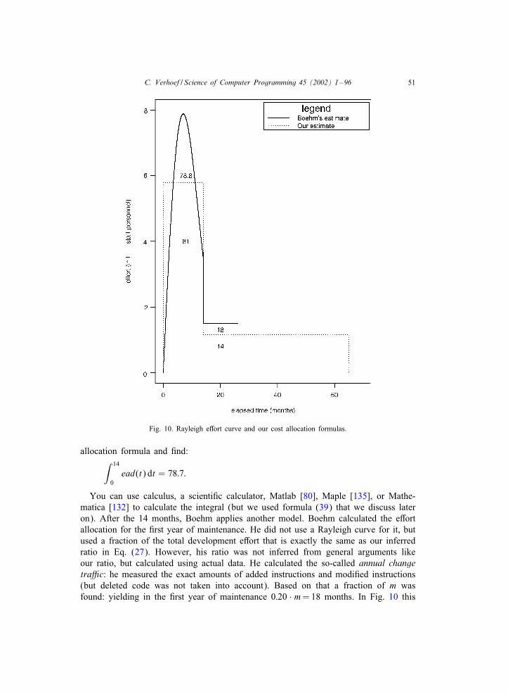
C. Verhoef / Science of Computer Programming 45 (2002) 1–96 51
Fig. 10. Rayleigh eOort curve and our cost allocation formulas.
allocation formula and Cnd:∫ 14
0ead(t) dt = 78:7:
You can use calculus, a scientiCc calculator, Matlab [80], Maple [135], or Mathe-matica [132] to calculate the integral (but we used formula (39) that we discuss lateron). After the 14 months, Boehm applies another model. Boehm calculated the eOortallocation for the Crst year of maintenance. He did not use a Rayleigh curve for it, butused a fraction of the total development eOort that is exactly the same as our inferredratio in Eq. (27). However, his ratio was not inferred from general arguments likeour ratio, but calculated using actual data. He calculated the so-called annual changetra@c: he measured the exact amounts of added instructions and modiCed instructions(but deleted code was not taken into account). Based on that a fraction of m wasfound: yielding in the Crst year of maintenance 0:20 · m= 18 months. In Fig. 10 this
52 C. Verhoef / Science of Computer Programming 45 (2002) 1–96
is expressed by the horizontal line at a height of 1.5 from the 14th to the 26th month.So the total eOort for the Crst 26 months of the project according to Boehm is 96.7man-months.
Let us compare this to our calculations for the level 1 case. The described projectis an MIS project: it is a raw material inventory project. So we can use formula (5),which is instantiated with an MIS schedule power. The number of staO necessary fordevelopment is nsd(14) = 5:8. Since it is a 14 month project, m= 81 man-months. Weplotted our eOort allocation function in Fig. 10 with a dashed line. Using formula (6),we can calculate the required staO for maintenance: nsm(14) = 1:16. This is the lowerhorizontal line that lasts for the entire life cycle of the system.
To compare our calculation to Boehm’s work, we take only the Crst year of main-tenance: m= 14 months. So the total eOort for development plus the Crst year ofoperation is 95 man-months. This is less than 2% diOerence with Boehm’s method.His method is clearly meant for CMM levels higher than 1. For, it is not feasible fora level 1 organization to measure the correct staO increase and decrease over time, thepeak eOort allocation, the number of added instructions, deleted instructions, modiCedinstructions, and so on.
From one example you cannot draw far reaching conclusions, but our approachmakes sense. Let’s have a second look at the general Rayleigh curve from Boehm’sbook. The area under a Rayleigh curve [102, p. 46] is exactly the total number ofman-months (we use formula (39) for this):∫ ∞
0ead(t) dt =
∫ ∞
0
mtp2 · e(−t2=2p2) dt
= m:
In our formulas, we abstract immediately from the staO variations, and treat thenumber of man-months for development as a constant over time. So the above deriva-tion shows that in general CMM level 2+ organizations will have more accurate dataover shorter time frames: with the Rayleigh curve you can predict for each moment intime, the exact eOort. While in our case, we use the average from the start, which co-incides with the area under the Rayleigh curve. The beneCt of having Rayleigh curvesis that you then Cnd a better average: not based on an external benchmark, but onactuals.
10. Towards full transparency
When you have the accumulated cost allocation curves for development and deploy-ment both for groups of projects and individual projects, you know the how, the when,and the how many of your IT-dollar expenditure. This adds to the badly needed trans-parency in IT performance and investments. In the previous section we have seen afew such curves already: a seismic IT impulse and an operational cost tsunami at theportfolio level. In all portfolios we analyzed, we encountered these two extremes pluscurves in between these extremes.
C. Verhoef / Science of Computer Programming 45 (2002) 1–96 53
10.1. Cost allocation equation
We note that our experience is limited to large companies: it may be the case thatdiOerent models are necessary in other cases. Based on our experience, we found thatIT portfolio costs over time can be accurately approximated by the following cost-time function c(t) returning for a given time t the corresponding cost. We conjecturethat this will also hold for IT portfolios that we have not assessed. Formula (38) forQIPM is
c(t) = a · t� · e−b·t� : (38)
In our formula a; �; b; � are constants idiosyncratic for the environment in which thework is carried out. Useful relations for the coeJcients can be inferred, as we will seelater on. Cost could be seen either as eOort, its corresponding Cnancial remuneration,or another cost dimension (see Fig. 11 for several plots of formula (38)).
It is already known for a long time that for �= 0 and �= 2 the above equation isused to estimate eOort allocation for research and development projects as shown byNorden [86–88]. Recall that for these � and � our cost allocation equation reduces tothe Rayleigh curve. After Norden, Putnam applied Rayleigh curves to software projects[100,103,101]. Also Boehm based his COCOMO model in part on Rayleigh curves.However, he noted that [6, p. 68]:
It is evident that the shape of the Rayleigh distribution in Fig. 5–5 is not aclose approximation to the shape of the labor distribution curves for any of theorganic-mode software projects shown in Fig. 5–4. This is largely because anorganic-mode software project generally starts with a good many of the projectmembers at work right away, instead of the slower buildup indicated by theRayleigh distribution. However, the central portion of the Rayleigh distributionprovides a good approximation to the labor curves of organic-mode softwareprojects.
Boehm thought that Rayleigh curves were not in accord with the actual costallocation of a certain type of project. So, Boehm used Rayleigh curves only aroundthe peak eOort p: between 0:3p and 1:7p. He could have used the so-called decen-tralized Rayleigh curve. If you need non-zero man power at the start of the project,you should use an additional location parameter, to shift the Rayleigh curve to theleft (use t − � instead of t). It is not necessary to invent another distribution for that.So by removing such a constraint it is possible to approximate reality much better.We did not display a decentralized version of our cost allocation function, but whenwe need it, this does not add any diJculty to using our results. Parr invented an al-ternative distribution for the same reason: a non-zero man power at the start of theproject [90]. Again, a decentralized Rayleigh distribution would have solved Parr’sissue satisfactorily (we discuss his distribution later on).
There are also cases where a Rayleigh curve is really not a good Ct for the givendata, including a decentralized version. Then the limitations of Rayleigh curves shouldnot function as a procrustean bed preventing accurate modeling of reality—when thatreality is just no Rayleigh curve. Indeed this was also found in a 2001 US Air Force
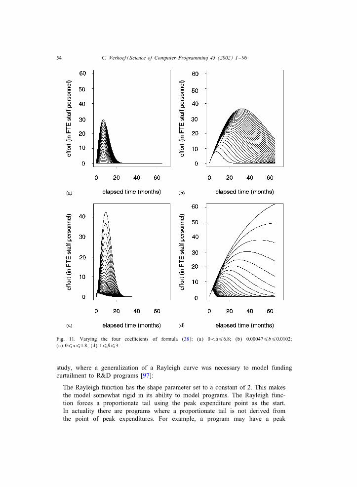
54 C. Verhoef / Science of Computer Programming 45 (2002) 1–96
Fig. 11. Varying the four coeJcients of formula (38): (a) 0¡a66:8; (b) 0:000476b60:0102;(c) 06�61:8; (d) 16�63.
study, where a generalization of a Rayleigh curve was necessary to model fundingcurtailment to R&D programs [97]:
The Rayleigh function has the shape parameter set to a constant of 2. This makesthe model somewhat rigid in its ability to model programs. The Rayleigh func-tion forces a proportionate tail using the peak expenditure point as the start.In actuality there are programs where a proportionate tail is not derived fromthe point of peak expenditures. For example, a program may have a peak
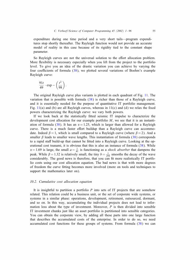
C. Verhoef / Science of Computer Programming 45 (2002) 1–96 55
expenditure during one time period and a very short tails—program expendi-tures stop shortly thereafter. The Rayleigh function would not provide an accuratemodel of reality in this case because of its rigidity tied to the constant shapeparameter.
So Rayleigh curves are not the universal solution to the eOort allocation problem.More Iexibility is necessary especially when you lift from the project to the portfoliolevel. To give you an idea of the drastic variation you can achieve by varying thefour coeJcients of formula (38), we plotted several variations of Boehm’s exampleRayleigh curve:
91t49
· exp−(t2
98
):
The original Rayleigh curve plus variants is plotted in each quadrant of Fig. 11. Thevariation that is possible with formula (38) is richer than those of a Rayleigh curve,and it is essentially needed for the purpose of quantitative IT portfolio management.Fig. 11(a) and (b) are all Rayleigh curves, whereas in 11(c) and (d) we relax the Cxedpowers characterizing the Rayleigh curve: we vary both powers.
If we look back at the statistically Ctted seismic IT impulse to characterize thedevelopment cost allocation for our example portfolio M , we see that it is an instanti-ation of formula (38). It has an �= 1:25, which is larger than allowed for a Rayleighcurve. There is a much faster eOort buildup than a Rayleigh curve can accommo-date. Indeed �= 1, which is small compared to a Rayleigh curve (where �= 2). And asmaller � leads to smaller wave lengths. This instantiation of formula (38) correspondsto a rapid staO build-up that cannot be Ctted into a Rayleigh curve. Looking at the op-erational cost tsunami, it is obvious that this is also an instance of formula (38). While�= 1:69 is large, the small a= 1
41 is functioning as a shock absorber that dampens thepeak. While �= 1:32 is relatively small, the tiny b= 1
294 smooths the decay of the waveconsiderably. The good news is therefore, that you can Ct more realistically IT portfo-lio costs using our cost allocation equation. The bad news is that with more degreesof freedom the curve Ctting becomes more involved (more on tools and techniques tosupport the mathematics later on).
10.2. Cumulative cost allocation equation
It is insightful to partition a portfolio P into sets of IT projects that are somehowrelated. This relation could be a business unit, or the set of corporate wide systems, orsystems in a similar phase: operations, development, retirement, outsourced, dormant,and so on. In this way, accumulating the individual projects does not lead to infor-mation loss about the type of investment. Moreover, P is then divided into sensibleIT investment chunks just like an asset portfolio is partitioned into sensible categories.You can obtain the corporate view, by adding all these parts into one large functionthat describes the accumulated costs of the enterprise. In order to do so, we needaccumulated cost functions for these groups of systems. From formula (38) we can
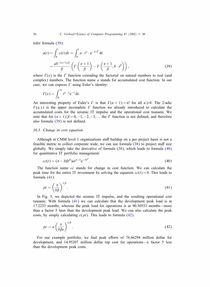
56 C. Verhoef / Science of Computer Programming 45 (2002) 1–96
infer formula (39):
a(t) =∫ t
0c(t) dt =
∫ t
0a · t� · e−b·t� dt
=ab−(�+1)=�
�
(�(� + 1�
)− �
(� + 1�
; b · t�))
; (39)
where �(x) is the � function extending the factorial on natural numbers to real (andcomplex) numbers. The function name a stands for accumulated cost function. In ourcase, we can express � using Euler’s identity:
�(x) =∫ ∞
0tx−1e−t dt:
An interesting property of Euler’s � is that �(n + 1) = n! for all n¿0. The 2-adic�(a; x) is the upper incomplete � function we already introduced to calculate theaccumulated costs for the seismic IT impulse and the operational cost tsunami. Wenote that for (� + 1)=�= 0;−1;−2;−3; : : : the � function is not deCned, and thereforealso formula (39) is not deCned.
10.3. Change in cost equation
Although at CMM level 1 organizations staO buildup on a per project basis is not afeasible metric to collect corporate wide, we can use formula (38) to project staO sizeglobally. We simply take the derivative of formula (38), which leads to formula (40)for quantitative IT portfolio management:
cc(t) = (�− b�t�)at�−1e−bt� : (40)
The function name cc stands for change in cost function. We can calculate thepeak time for the entire IT investment by solving the equation cc(t) = 0. This leads toformula (41):
pt =(
�b�
)1=�
: (41)
In Fig. 5, we depicted the seismic IT impulse, and the resulting operational costtsunami. With formula (41) we can calculate that the development peak load is at17.2233 months, whereas the peak load for operations is at 90.30533 months—morethan a factor 5 later than the development peak load. We can also calculate the peakcosts, by simply calculating c(pt). This leads to formula (42):
pc = a(
�b�e
)�=�
: (42)
For our example portfolio, we Cnd peak eOorts of 76.66294 million dollar fordevelopment, and 14.95207 million dollar top cost for operations—a factor 5 lessthan the development peak costs.
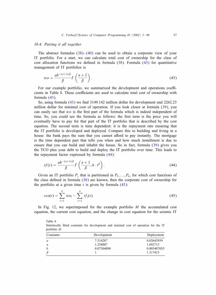
C. Verhoef / Science of Computer Programming 45 (2002) 1–96 57
10.4. Putting it all together
The abstract formulas (38)–(40) can be used to obtain a corporate view of yourIT portfolio. For a start, we can calculate total cost of ownership for the class ofcost allocation functions we deCned in formula (38). Formula (43) for quantitativemanagement of IT portfolios is
tco =ab−(�+1)=�
��(� + 1�
): (43)
For our example portfolio, we summarized the development and operations coeJ-cients in Table 8. These coeJcients are used to calculate total cost of ownership withformula (43).
So, using formula (43) we Cnd 3149.142 million dollar for development and 2262.23million dollar for minimal cost of operation. If you look closer at formula (39), youcan easily see that tco is the Crst part of the formula which is indeed independent oftime. So, you could see the formula as follows: the Crst term is the price you willeventually have to pay for that part of the IT portfolio that is described by the costequation. The second term is time dependent: it is the repayment rate ensuring thatthe IT portfolio is developed and deployed. Compare this to building and living in ahouse: the bank pays the sum that you cannot aOord to pay instantly. The mortgageis the time dependent part that tells you when and how much installment is due toensure that you can build and inhabit the house. So in fact, formula (39) gives youthe TCO plus your debt to build and deploy the IT portfolio over time. This leads tothe repayment factor expressed by formula (44):
rf (t) =ab−(�+1)=�
��(� + 1�
; b · t�): (44)
Given an IT portfolio P, that is partitioned in P1; : : : ; Pn, for which cost functions ofthe class deCned in formula (38) are known, then the corporate cost of ownership forthe portfolio at a given time t is given by formula (45):
cco(t) =n∑
i=1
tcoi −n∑
i=1
rf i(t): (45)
In Fig. 12, we superimposed for the example portfolio M the accumulated costequation, the current cost equation, and the change in cost equation for the seismic IT
Table 8Statistically Ctted constants for development and minimal cost of operation for the ITportfolio M .
Constants Development Deployment
a 7.514287 0.02643959� 1.258007 1.692713b 0.07304098 0.003407055� 1 1.317413
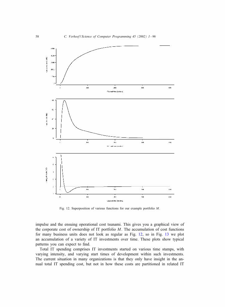
58 C. Verhoef / Science of Computer Programming 45 (2002) 1–96
Fig. 12. Superposition of various functions for our example portfolio M .
impulse and the ensuing operational cost tsunami. This gives you a graphical view ofthe corporate cost of ownership of IT portfolio M . The accumulation of cost functionsfor many business units does not look as regular as Fig. 12, so in Fig. 13 we plotan accumulation of a variety of IT investments over time. These plots show typicalpatterns you can expect to Cnd.
Total IT spending comprises IT investments started on various time stamps, withvarying intensity, and varying start times of development within such investments.The current situation in many organizations is that they only have insight in the an-nual total IT spending cost, but not in how these costs are partitioned in related IT
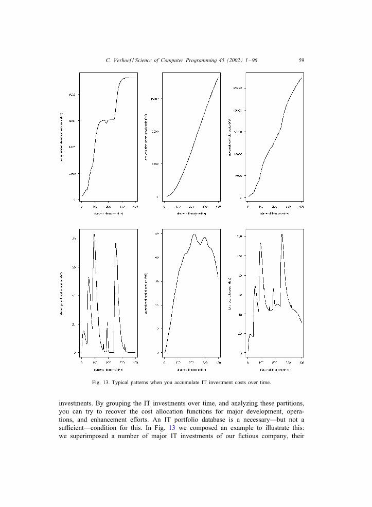
C. Verhoef / Science of Computer Programming 45 (2002) 1–96 59
Fig. 13. Typical patterns when you accumulate IT investment costs over time.
investments. By grouping the IT investments over time, and analyzing these partitions,you can try to recover the cost allocation functions for major development, opera-tions, and enhancement eOorts. An IT portfolio database is a necessary—but not asuJcient—condition for this. In Fig. 13 we composed an example to illustrate this:we superimposed a number of major IT investments of our Cctious company, their
60 C. Verhoef / Science of Computer Programming 45 (2002) 1–96
ensuing operational costs plus their enhancement costs. Some of them can be rec-ognized by their peaks, others are faded out by the more dominating waves. Theleft-hand plot in the upper row of Fig. 13 shows the accumulation of all the develop-ment costs over time for the IT investments. The middle plot represents accumulatedoperational costs over time, and the right-hand plot is their sum: the total accumu-lated costs. The lower row plots the cost allocations for the IT investments. Theyare the cost allocation for development, operational and enhancement costs, and theirsum. These accumulations give less insight in how the costs are build-up than if youwould have had the cost allocation functions from the onset. The challenge is to un-cover the cost allocation formulas from the data that is collected in the IT portfoliodatabase. This is not an easy task, and there is no guarantee that you can completelyrecover the actual cost allocation formulas that belong to the IT investments of thepast. The major investments leave so many traces that their recovery is often withinreach. They are the cost waves from the past that are still dominating the currentbudgets.
11. Quantitative support for decision making
Next we turn our attention to how quantitative information can support decisionmaking. Of course, the entire decision making process comprises of many factors, ofwhich quantitative input is one aspect. Currently, not much quantitative data supportsstrategic decisions on IT investments. We agree with Strassmann who writes on thistopic [122, p. 261]:
Credible Cnancial analyses are necessary before top management can act with anunderstanding of the consequences of any decision.
We elaborate on quantitative support for a decision that many executives face whenIT investments are due: outsourcing or not? For many organizations owning serioussized IT portfolios it is not possible to construct and maintain all the software in-house. So this is partly an in-house matter, and partly taken care of externally. At theexecutive level, decisions should be made to that end, and quantitative support willhelp in making the most eOective decisions. There are the following possibilities forIT systems or IT portfolios:
• Make. This implies that you start (or restart) to make the software from scratch,and you are going to do this within the organization.
• Buy. This implies that the functionality can be bought oO-the-shelf from an inde-pendent software vendor.
• Commission. This implies that you commission an outsourcer to build the desiredfunctionality.
• Renovate. This implies that there is an existing software asset within yourorganization and that you want to renovate this to develop the desired func-tionality.
• Wait. This means that you postpone to decide on any of the above.
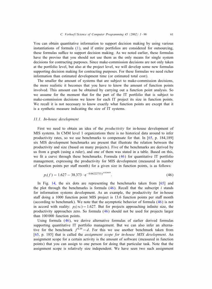
C. Verhoef / Science of Computer Programming 45 (2002) 1–96 61
You can obtain quantitative information to support decision making by using variousinstantiations of formula (1), and if entire portfolios are considered for outsourcing,these formulas suJce to support decision making. As we noted earlier, these formulashave the proviso that you should not use them as the only means for single systemdecisions for contracting purposes. Since make-commission decisions are not only takenat the portfolio level, but also at the project level, we will develop some new formulassupporting decision making for contracting purposes. For these formulas we need richerinformation than estimated development time (or estimated total cost).
The smaller the amount of systems that are subject to make-commission decisions,the more realistic it becomes that you have to know the amount of function pointsinvolved. This amount can be obtained by carrying out a function point analysis. Sowe assume for the moment that for the part of the IT portfolio that is subject tomake-commission decisions we know for each IT project its size in function points.We recall it is not necessary to know exactly what function points are except that itis a synthetic measure indicating the size of IT systems.
11.1. In-house development
First we need to obtain an idea of the productivity for in-house development ofMIS systems. In CMM level 1 organizations there is no historical data around to inferproductivity rates, so we use benchmarks to compensate for that. In [65, p. 184,189]six MIS development benchmarks are present that illustrate the relation between theproductivity and size (based on many projects). Five of the benchmarks are derived byus from a graph (using a ruler), and one of them was stated in a table. Based on this,we Ct a curve through these benchmarks. Formula (46) for quantitative IT portfoliomanagement, expressing the productivity for MIS development (measured in numberof function points per staO month) for a given size in function points, is as follows:
pi(f) = 1:627 − 38:373 · e−0:06222733f0:424459: (46)
In Fig. 14, the six dots are representing the benchmarks taken from [65] andthe plot through the benchmarks is formula (46). Recall that the subscript i standsfor information systems development. As an example, the productivity for in-housestaO doing a 1000 function point MIS project is 13.6 function points per staO month(according to benchmark). We note that the asymptotic behavior of formula (46) is notin accord with reality: pi(∞) = 1:627. But for projects approaching inCnite size, theproductivity approaches zero. So formula (46) should not be used for projects largerthan 100 000 function points.
Using formula (46), we derive alternative formulas of earlier derived formulassupporting quantitative IT portfolio management. But we can also infer an alterna-tive for the benchmark f0:39 =d. For this we use another benchmark taken from[65, p. 185] that is called the assignment scope for in-house MIS development. Anassignment scope for a certain activity is the amount of software (measured in functionpoints) that you can assign to one person for doing that particular task. Note that theassignment scope is relatively size independent. We have seen two such assignment
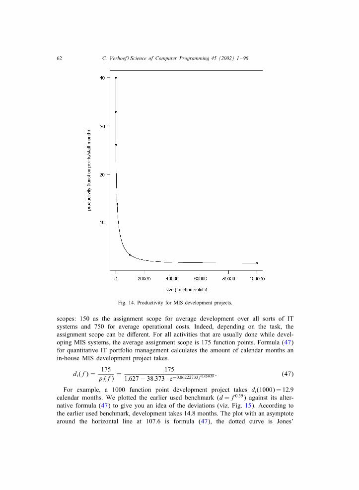
62 C. Verhoef / Science of Computer Programming 45 (2002) 1–96
Fig. 14. Productivity for MIS development projects.
scopes: 150 as the assignment scope for average development over all sorts of ITsystems and 750 for average operational costs. Indeed, depending on the task, theassignment scope can be diOerent. For all activities that are usually done while devel-oping MIS systems, the average assignment scope is 175 function points. Formula (47)for quantitative IT portfolio management calculates the amount of calendar months anin-house MIS development project takes.
di(f) =175pi(f)
=175
1:627 − 38:373 · e−0:06222733f0:424459 : (47)
For example, a 1000 function point development project takes di(1000) = 12:9calendar months. We plotted the earlier used benchmark (d=f0:39) against its alter-native formula (47) to give you an idea of the deviations (viz. Fig. 15). According tothe earlier used benchmark, development takes 14.8 months. The plot with an asymptotearound the horizontal line at 107.6 is formula (47), the dotted curve is Jones’
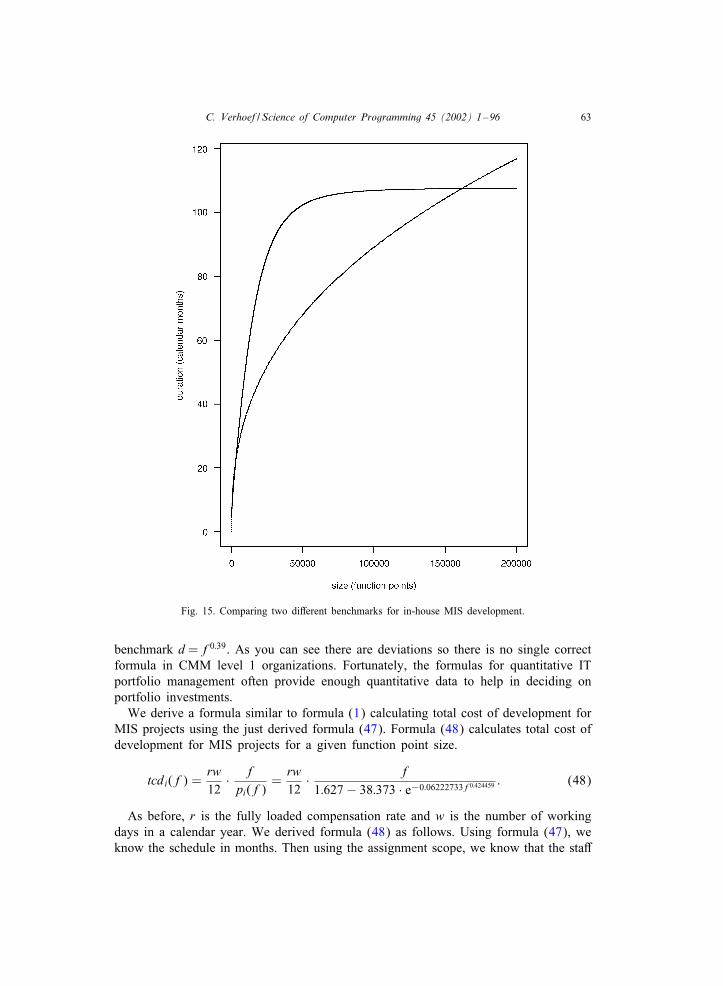
C. Verhoef / Science of Computer Programming 45 (2002) 1–96 63
Fig. 15. Comparing two diOerent benchmarks for in-house MIS development.
benchmark d=f0:39. As you can see there are deviations so there is no single correctformula in CMM level 1 organizations. Fortunately, the formulas for quantitative ITportfolio management often provide enough quantitative data to help in deciding onportfolio investments.
We derive a formula similar to formula (1) calculating total cost of development forMIS projects using the just derived formula (47). Formula (48) calculates total cost ofdevelopment for MIS projects for a given function point size.
tcdi(f) =rw12
· fpi(f)
=rw12
· f1:627 − 38:373 · e−0:06222733f0:424459 : (48)
As before, r is the fully loaded compensation rate and w is the number of workingdays in a calendar year. We derived formula (48) as follows. Using formula (47), weknow the schedule in months. Then using the assignment scope, we know that the staO
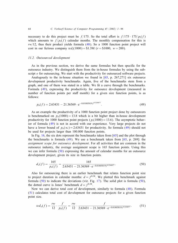
64 C. Verhoef / Science of Computer Programming 45 (2002) 1–96
necessary to do this project must be f=175. So the total eOort is f=175 · 175=pi(f)which amounts to f=pi(f) calendar months. The monthly compensation for this isrw=12, thus their product yields formula (48). So a 1000 function point project willcost in our Cctious company tcdi(1000) = $1:3M (r = $1000; w= 200).
11.2. Outsourced development
As in the previous section, we derive the same formulas but then speciCc for theoutsource industry. We distinguish them from the in-house formulas by using the sub-script o for outsourcing. We start with the productivity for outsourced software projects.
Analogously to the in-house situation we found in [65, p. 267,271] six outsourcedevelopment productivity benchmarks. Again, Cve of the benchmarks stem from agraph, and one of them was stated in a table. We Ct a curve through the benchmarks.Formula (49), expressing the productivity for outsource development (measured innumber of function points per staO month) for a given size function points, is asfollows:
po(f) = 2:63431 − 21:36569 · e−0:01805819f0:5248877: (49)
As an example the productivity of a 1000 function point project done by outsourcersis benchmarked on po(1000) = 13:8 which is a bit higher than in-house developmentproductivity for 1000 function point projects (pi(1000) = 13:6). The asymptotic behav-ior of formula (49) is not in accord with our experience. Very large projects do nothave a lower bound of po(∞) = 2:63431 for productivity. So formula (49) should notbe used for projects larger than 100.000 function points.
In Fig. 16, the six dots represent the benchmarks taken from [65] and the plot throughthe benchmarks is formula (49). We use a benchmark taken from [65, p. 269]: theassignment scope for outsource development. For all activities that are common in theoutsource industry, the average assignment scope is 165 function points. Using thiswe can infer formula (50) expressing the amount of calendar months for an outsourcedevelopment project, given its size in function points.
do(f) =165
po(f)=
1652:63431 − 21:36569 · e−0:01805819f0:5248877 : (50)
Also for outsourcing there is an earlier benchmark that relates function point sizeto project duration in calendar months: d=f0:38. We plotted this benchmark againstformula (50) to indicate the deviations (viz. Fig. 17). The solid plot is formula (50),the dotted curve is Jones’ benchmark d=f0:38.
Now we can derive total cost of development, similarly to formula (48). Formula(51) calculates total cost of development for outsource projects for a given functionpoint size.
tcdo(f) =rw12
· fpo(f)
=rw12
· f2:63431 − 21:36569 · e−0:01805819f0:5248877 : (51)
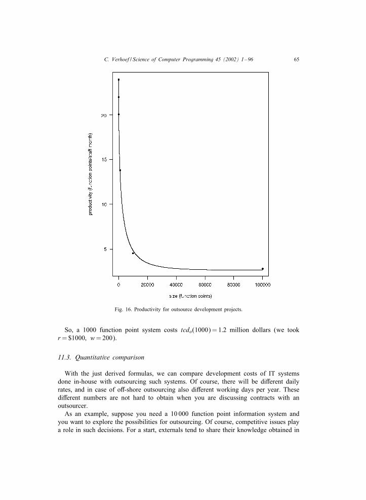
C. Verhoef / Science of Computer Programming 45 (2002) 1–96 65
Fig. 16. Productivity for outsource development projects.
So, a 1000 function point system costs tcdo(1000) = 1:2 million dollars (we tookr = $1000; w= 200).
11.3. Quantitative comparison
With the just derived formulas, we can compare development costs of IT systemsdone in-house with outsourcing such systems. Of course, there will be diOerent dailyrates, and in case of oO-shore outsourcing also diOerent working days per year. ThesediOerent numbers are not hard to obtain when you are discussing contracts with anoutsourcer.
As an example, suppose you need a 10 000 function point information system andyou want to explore the possibilities for outsourcing. Of course, competitive issues playa role in such decisions. For a start, externals tend to share their knowledge obtained in
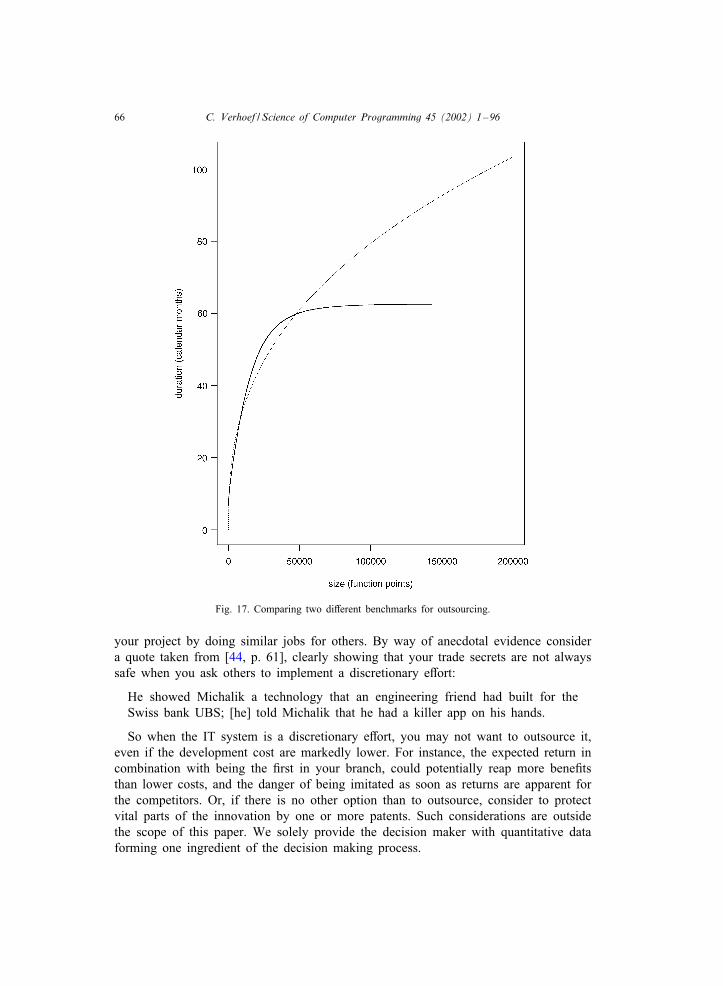
66 C. Verhoef / Science of Computer Programming 45 (2002) 1–96
Fig. 17. Comparing two diOerent benchmarks for outsourcing.
your project by doing similar jobs for others. By way of anecdotal evidence considera quote taken from [44, p. 61], clearly showing that your trade secrets are not alwayssafe when you ask others to implement a discretionary eOort:
He showed Michalik a technology that an engineering friend had built for theSwiss bank UBS; [he] told Michalik that he had a killer app on his hands.
So when the IT system is a discretionary eOort, you may not want to outsource it,even if the development cost are markedly lower. For instance, the expected return incombination with being the Crst in your branch, could potentially reap more beneCtsthan lower costs, and the danger of being imitated as soon as returns are apparent forthe competitors. Or, if there is no other option than to outsource, consider to protectvital parts of the innovation by one or more patents. Such considerations are outsidethe scope of this paper. We solely provide the decision maker with quantitative dataforming one ingredient of the decision making process.
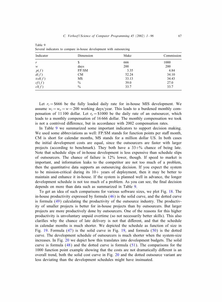
C. Verhoef / Science of Computer Programming 45 (2002) 1–96 67
Table 9Several indicators to compare in-house development with outsourcing
Indicator Dimension Make Commission
r $ 666 1000w days 200 200p(f) FP=SM 3.35 4.84d(f) CM 52.24 34.10tcd(f) M$ 33.13 34.43cf (f) % 39.0 27.0cl(f) % 33.7 33.7
Let ri = $666 be the fully loaded daily rate for in-house MIS development. Weassume wi =wo =w= 200 working days=year. This leads to a burdened monthly com-pensation of 11100 dollar. Let ro = $1000 be the daily rate of an outsourcer, whichleads to a monthly compensation of 16 666 dollar. The monthly compensation we tookis not a contrived diOerence, but in accordance with 2002 compensation rates.
In Table 9 we summarized some important indicators to support decision making.We used some abbreviations as well: FP=SM stands for function points per staO month,CM is short for calendar months, M$ stands for a million dollar US. In both casesthe initial development costs are equal, since the outsourcers are faster with largerprojects (according to benchmark). They both have a 33+% chance of being late.Note that schedule slips of in-house development is less expensive than schedule slipsof outsourcers. The chance of failure is 12% lower, though. If speed to market isimportant, and information leaks to the competitor are not too much of a problem,then the quantitative data supports an outsourcing decision. If you expect the systemto be mission-critical during its 10+ years of deployment, then it may be better tomaintain and enhance it in-house. If the system is planned well in advance, the longerdevelopment schedule is not too much of a problem. As you can see, the Cnal decisiondepends on more than data such as summarized in Table 9.
To get an idea of such comparisons for various software sizes, we plot Fig. 18. Thein-house productivity expressed by formula (46) is the solid curve, and the dotted curveis formula (49) calculating the productivity of the outsource industry. The productiv-ity of smaller projects is better for in-house projects than by outsourcers. But largerprojects are more productively done by outsourcers. One of the reasons for this higherproductivity is unvoluntary unpaid overtime (so not necessarily better skills). This alsoclariCes why the chance of late delivery is not that diOerent, and that the schedulein calendar months is much shorter. We depicted the schedule as function of size inFig. 19. Formula (47) is the solid curve in Fig. 19, and formula (50) is the dottedcurve. The development schedule of outsourcers is much shorter when the system-sizeincreases. In Fig. 20 we depict how this translates into development budgets. The solidcurve is formula (48) and the dotted curve is formula (51). The comparisons for the1000 function point example showing that the costs are not dramatically diOerent is anoverall trend, both the solid cost curve in Fig. 20 and the dotted outsource variant areless deviating than the development schedules might have insinuated.
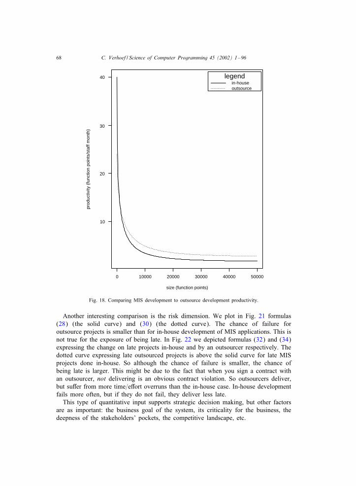
68 C. Verhoef / Science of Computer Programming 45 (2002) 1–96
size (function points)
prod
uctiv
ity (
func
tion
poin
ts/s
taff
mon
th)
0 10000 20000 30000 40000 50000
10
20
30
40 legendin-houseoutsource
Fig. 18. Comparing MIS development to outsource development productivity.
Another interesting comparison is the risk dimension. We plot in Fig. 21 formulas(28) (the solid curve) and (30) (the dotted curve). The chance of failure foroutsource projects is smaller than for in-house development of MIS applications. This isnot true for the exposure of being late. In Fig. 22 we depicted formulas (32) and (34)expressing the change on late projects in-house and by an outsourcer respectively. Thedotted curve expressing late outsourced projects is above the solid curve for late MISprojects done in-house. So although the chance of failure is smaller, the chance ofbeing late is larger. This might be due to the fact that when you sign a contract withan outsourcer, not delivering is an obvious contract violation. So outsourcers deliver,but suOer from more time=eOort overruns than the in-house case. In-house developmentfails more often, but if they do not fail, they deliver less late.
This type of quantitative input supports strategic decision making, but other factorsare as important: the business goal of the system, its criticality for the business, thedeepness of the stakeholders’ pockets, the competitive landscape, etc.
C. Verhoef / Science of Computer Programming 45 (2002) 1–96 69
size (function points)
deve
lopm
ent t
ime
(cal
enda
r m
onth
s)
0 20000 40000 60000 80000 100000
20
40
60
80
100
legendin-houseoutsourced
Fig. 19. Comparing MIS development to outsource development schedules.
12. Cost--time analysis and lifetime analysis
We could develop many more formulas for quantitative IT portfolio management,supporting strategic decision making for IT portfolios and sanity checking on ITprojects. But at this point we think it is worthwhile to turn our attention to a morefundamental issue. It is the issue whether it is possible to incorporate our empiricallyfound formulas within an existing body of mathematical and statistical knowledge. For,if we are able to connect our work to established theory, we can beneCt from Cndingsin that area, and insights from these areas could lead to insights in the formulas wedeveloped thus far. Others have tried to connect quantitative IT portfolio managementto modern portfolio theory, and we showed that this correspondence is not as promisingas it seemed at Crst.
After a careful study of our empirically found formulas we are conCdent to havefound this existing body of knowledge. It is called lifetime analysis or failure time
70 C. Verhoef / Science of Computer Programming 45 (2002) 1–96
size (function points)
cost
s (m
illio
ns o
f dol
lars
)
0 20000 40000 60000 80000 100000
0
200
400
600
legendin-houseoutsourced
Fig. 20. Comparing MIS development to outsource development costs.
analysis as is applied to cancer research, cure rate estimation, reliability analysis, andother areas ranging from returns on the NYSE to the physical laws that the crushingof coal are subject to. This analysis will follow shortly, and it made us think of ourwork as cost–time analysis.
In the practical software engineering area, there is no established tradition of mathe-matically describing important phenomena in order to control the engineering process,and the ensuing artifacts [76,43]. In part this is due to the fact that the mathematicsis not closely connected to obvious applications that are of immediate use in practice.For Celds where this is obvious, such as software cost estimation, not many peoplerelate their work to common practice in mathematics or statistics. Let us illustrate this.Recall Boehm [6] and Parr [90] who go to great length to infer alternatives to Rayleighdistributions whereas they could have used a decentralized version. Another indicationis the ongoing discussion how useful mathematics is for the software practitioner. We
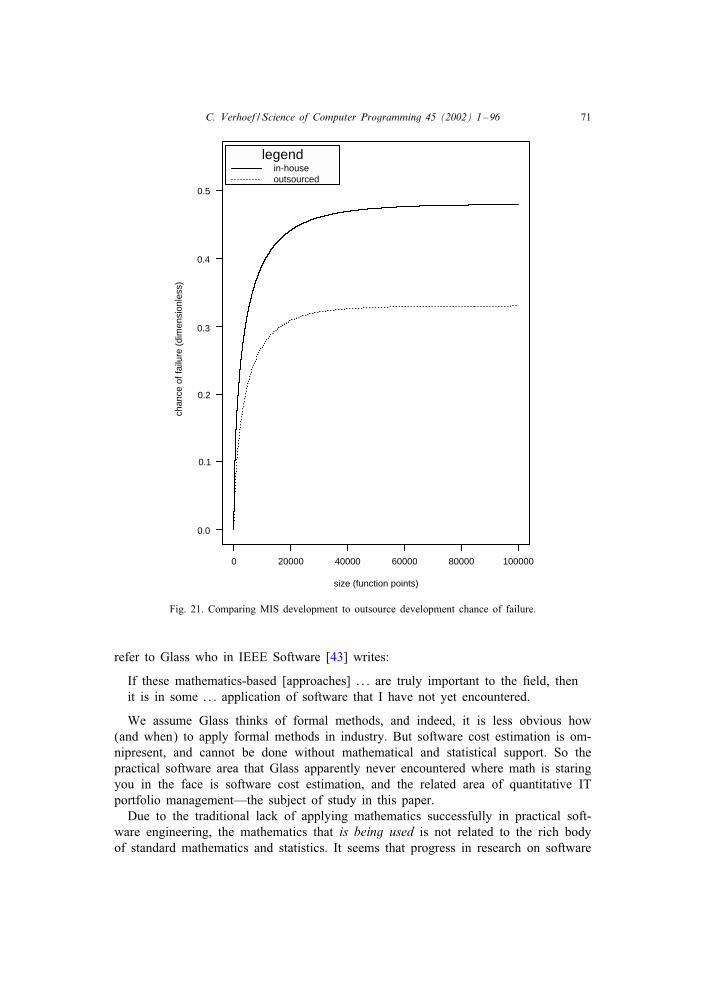
C. Verhoef / Science of Computer Programming 45 (2002) 1–96 71
size (function points)
chan
ce o
f fai
lure
(di
men
sion
less
)
0 20000 40000 60000 80000 100000
0.0
0.1
0.2
0.3
0.4
0.5
legendin-houseoutsourced
Fig. 21. Comparing MIS development to outsource development chance of failure.
refer to Glass who in IEEE Software [43] writes:
If these mathematics-based [approaches] : : : are truly important to the Celd, thenit is in some : : : application of software that I have not yet encountered.
We assume Glass thinks of formal methods, and indeed, it is less obvious how(and when) to apply formal methods in industry. But software cost estimation is om-nipresent, and cannot be done without mathematical and statistical support. So thepractical software area that Glass apparently never encountered where math is staringyou in the face is software cost estimation, and the related area of quantitative ITportfolio management—the subject of study in this paper.
Due to the traditional lack of applying mathematics successfully in practical soft-ware engineering, the mathematics that is being used is not related to the rich bodyof standard mathematics and statistics. It seems that progress in research on software
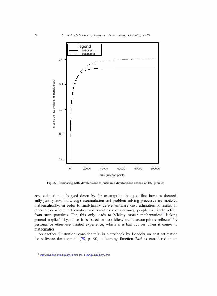
72 C. Verhoef / Science of Computer Programming 45 (2002) 1–96
size (function points)
chan
ce o
n la
te p
roje
cts
(dim
ensi
onle
ss)
0 20000 40000 60000 80000 100000
0.0
0.1
0.2
0.3
0.4
legendin-houseoutsourced
Fig. 22. Comparing MIS development to outsource development chance of late projects.
cost estimation is bogged down by the assumption that you Crst have to theoreti-cally justify how knowledge accumulation and problem solving processes are modeledmathematically, in order to analytically derive software cost estimation formulas. Inother areas where mathematics and statistics are necessary, people explicitly refrainfrom such practices. For, this only leads to Mickey mouse mathematics 3 lackinggeneral applicability, since it is based on too idiosyncratic assumptions reIected bypersonal or otherwise limited experience, which is a bad advisor when it comes tomathematics.
As another illustration, consider this: in a textbook by Londeix on cost estimationfor software development [78, p. 90] a learning function 2atn is considered in an
3 www.mathematicallycorrect.com/glossary.htm
C. Verhoef / Science of Computer Programming 45 (2002) 1–96 73
exercise for which the manpower distribution and cumulative manpower cost are tobe calculated. Londeix rejects this particular distribution on the following grounds [78,p. 195]:
We can verify that when n increases the time scale is reduced. An increase of ngives a sharp rise of the peak manning relative to its value for n= 1. Therefore,a non-linear learning curve would give an early more peaky model which wouldnot be helpful to represent the reality of software development.
This is further justiCed in the textbook by a reference to Norden’s model [88]: sinceNorden is using a linear learning curve, the nonlinear learning curve cannot be correct.Needless to say that this line of reasoning is erroneous. A learning curve can neverbe inappropriate because someone else is using a diOerent curve. Irrespective of hisline or reasoning, Londeix is mistaken: we know from empirical research reported onin [97] that nonlinear learning curves accurately model IT intensive programs. Theonly limitation that Londeix should have questioned is that the assumption that n is anatural number is too restrictive.
So the general tendency in software cost estimation is to Crst restrict one selves andwithin those limitations try to model cost estimation phenomena. This is the wrongordering as we will argue below.
12.1. Ready, 7re, aim
In general it is not smart to Cx a speciCc (theoretical) cost–time model inadvance—and then see if this assumption Cts reality. Unless the theoretical deriva-tion is conclusive, this should always be done the other way around: you decide ona—hopefully general enough—family of distributions, and by curve Ctting the mostlikely distribution for that particular eOort will turn up as the result of statisticalanalysis.
The Cxed-model approach is not the way to go when you just want to control thingsaccurately, but this ready-Cre-aim approach seems the norm in software engineering.It is much better to skip the motivational part all together, and instead do an educatedguess that the relation you wish to describe probably Cts a very general family ofdistributions like our family of cost allocation functions (38) is fortuitously doing. Ordiscriminate among several parametric models, to see which one should be used atall [99]. To quote Lawless [75, p. 13], who touches upon this issue in the realm oflifetime analysis:
Extensive motivation is not provided for the various models. To do this wouldrequire a thorough discussion of aging and failure processes and would takeus outside the book’s intended subject area. Indeed, the motivation for using aparticular model in a given situation is often mainly empirical, it having beenfound that the model satisfactorily describes the distribution of lifetimes in thepopulation under study. This does not imply any absolute “correctness” of themodel.
74 C. Verhoef / Science of Computer Programming 45 (2002) 1–96
KalbIeisch and Prentice go a step further, when they write about failure time dataanalysis [67, p. 3]:
In many situations it is also important to develop nonparametric and robust pro-cedures since there is frequently little empirical or theoretical work to supporta particular family of failure time distributions.
They even indicate that you might question the assumption that there would be ananalytic relation at all. We are in complete agreement with the observations done byLawless, KalbIeisch, and Prentice.
Also consider this: there can be some time between empirically found mathematicaltools and their formal underpinning. For instance, the so-called Weibull distributionwas empirically found in 1933 by Rosin and Rammler to describe the crushing ofcoal [107] (it was later attributed to Weibull [131]). However, the Crst full theoreticalderivation based on physical principles stems from 1995 [14]. In the mean time, thedistribution has been very instrumental in lifetime analysis [75].
The statistical ready-Cre-aim practice is not unique to software engineering. Thisissue is also noted in other areas. For instance, in the realm of cure rate estimation inclinical trials for diseases such as lymphoma and breast cancer, similar critical remarks,eloquently expressing the viewpoints of [67, p. 67], are made [94]:
In the last decade, mixture models under diOerent distributions, such as expo-nential, Weibull, log-normal and Gompertz, have been discussed and used. How-ever, these models involve stronger distributional assumptions than is desirableand inferences may not be robust to departures from these assumptions. In thispaper, a mixture model is proposed using the generalized F distribution family. Al-though this family is seldom used because of computational diJculties, it has theadvantage of being very Iexible and including many commonly used distributionsas special cases. The generalised F mixture model can relax the usual strongerdistributional assumptions and allow the analyst to uncover structure in the datathat might otherwise have been missed.
Indeed, using Cxed or restricted families of distributions also restricts the possibilityto Ct your data, and as the authors of [67,94] correctly observe, using a general distri-bution, you can uncover structure in your data that with a restricted model is missed.The generalized F distribution was originally intended as a selection process to detectwhich known less general distribution Cts data most appropriately [99].
So, instead of trying to unravel why a particular curve is appropriate to model acorrelation you can better skip that part for later and readily begin to Ct curves thatare approximating the relation accurately. Any formula, satisfying your purpose is bydeCnition useful—the answer why this formula does Ct is just a nice-to-have. As youwill see shortly, it turns out to be utterly useful to relate our cost–time formulas toestablished practice in statistical modeling.
12.2. The generalized � distribution
In order to do so, it is necessary to turn formula (38) into a so-called probabil-ity density function. We normalize formula (38) so that the area under the curve
C. Verhoef / Science of Computer Programming 45 (2002) 1–96 75
becomes 1, by dividing formula (38) by the area under it. We use formula (39) forthis. Formula (52) is the probability density function variant of formula (38):
f(t) =�b(�+1)=�
�(� + 1=�)· t�e−bt� : (52)
Formula (53) is the cumulative distribution function belonging to formula (52):
F(t) = 1 − �((� + 1)=�; bt�)�((� + 1)=�)
: (53)
Indeed normalization means that F(∞) = 1, which is not hard to check. Now wecan easily relate formulas (52) and (53) to established statistical tools.
Theorem 1. Formula (52) is equivalent to the generalized � distribution [115].
The generalized � distribution is deCned as follows:
g(t) =�
�(k) · "( t"
)k�−1e−(t=")� :
If we take � = �k − 1 and b = 1="�, we can easily Cnd that formula (52) turns intothe generalized � distribution. Vice versa, if we take k = (� + 1)=� and " = (1=b)1=�,this reduces the generalized � distribution to formula (52). So, both distributions arethe same.
Obviously then also all the other artifacts coincide, e.g., their cumulative distributionfunctions are the same.
12.3. Lifetime data analysis
So now we have related our normalized empirically found cost–time family ofrelations to an existing family for which there are tools and techniques available thatwe can borrow to eOectively deal with the practical side of applying the necessarystatistical analyses. This Celd is not modern portfolio theory, but lifetime data analysis.
In the 1930s functions similar to the generalized � distribution were used to theanalyze the distribution of economic income [2,25]. But also in 2001, it was shown thatstock returns on the New York Stock Exchange can be approximated by a generalizedlog gamma distribution [11]. So there are relations between quantitative IT portfoliomanagement and the returns on stock options, but as argued, these relations are notwhat you would expect, namely that security portfolio theory founded by Markowitzcorresponds in some natural way to issues relevant for IT portfolios.
A major application Celd of the generalized � distribution is in the so-called lifetimedata analysis [75]. This branch of statistics is also referred to as survival time, or failuretime analysis [67] and is widely used in engineering to support reliability analysis, andin the biomedical sciences. While the notion of lifetime should be taken literally, e.g.,in biomedical science, in other Celds it merely indicates a non-negative-valued variable.Our application comprises cost–time analysis for IT portfolios. There is a one-to-one
76 C. Verhoef / Science of Computer Programming 45 (2002) 1–96
correspondence with concepts from lifetime analysis, and the Celd of software costestimation, in particular quantitative IT portfolio management.
Let us Crst review the few most basic concepts of lifetime data analysis (this infor-mation can be found in any book on lifetime data analysis), so that we can illustratethe strong correspondence with IT cost issues. Suppose T is a nonnegative randomvariable representing a lifetime, e.g., of individuals in a population. Let f(t) be theprobability density function of T . Then the distribution function F(t) is deCned asfollows:
F(t) = P(T 6 t) =∫ t
0f(x) dx;
where P(T6t) denotes the chance that the lifetime T is between zero and t. Thesurvival function is deCned as
S(t) = P(T ¿ t) =∫ ∞
tf(x) dx:
As we can see, when t→∞, then the distribution function F will approach 1,whereas the survival function will approach zero: S(∞) = 0. In other words, it becomesharder and harder to survive when time proceeds. An important notion in lifetimeanalysis is the so-called hazard function, also known as the hazard rate, the age-speciCcfailure rate, or the more poetic name: force of mortality:
h(t) =f(t)S(t)
:
The hazard function expresses the instantaneous death rate at time t given that thereis survival up till t. The hazard rate thus describes the way in which the instantaneousdeath of an individual (or the failure of some device) changes with time. So whenyou follow subjects from birth to death the hazard rate can be a bathtub curve: rightafter materialization there can be childhood diseases, then a relatively constant rate,and then the rate will go up again. The cumulative hazard function is easily deCned:
H (t) =∫ t
0h(x) dx:
With these basic deCnitions it is possible to derive a number of fundamental relationsbetween the various notions. For a start, the probability density function can be writtenas a product of two intuitive functions:
f(t) = h(t) · S(t);
and since f=− S ′, it is not hard to Cnd that
S(t) = e−∫ t
0h(x) dx:
Combining the above two formulas:
f(t) = h(t) · e−∫ t
0h(x) dx:
C. Verhoef / Science of Computer Programming 45 (2002) 1–96 77
So, the hazard function can serve as a means to derive the probability densityfunction. For instance, suppose that the hazard function is constant: h(t) = %. Thenthe probability density function is f(t) = %e−%t , which is the exponential or Poissondistribution that is often used in reliability and lifetime analysis.
12.4. Correspondence to software cost estimation
Let us give a second example, to start showing the one-to-one correspondence.Norden presupposed that the eOectiveness of a group of engineers increases progres-sively during the life cycle of a project that he represented by a function p(t), wherethe p is an abbreviation for the problem function indicating the level of skill availableto solve the problems. He assumes this function to be linear. In fact the function pis what in lifetime analysis is called the hazard function. Norden, thus assumes a lin-ear hazard rate. With the basic formulas for lifetime analysis, Cnding the probabilitydensity function is obvious:
f(t) = ate−at2=2:
This is the Rayleigh distribution that Norden derived, using diOerential calculus.In lifetime analysis, the Rayleigh distribution is also known as the linear hazard ratedistribution [4,71].
In the paper [90], Parr proposed an alternative to the Rayleigh distribution toestimate software costs. This model is sometimes called the sech square model dueto its formulation:
V (t) = (1=4)sech2((�t + c3)=2):
We note that sech(x) = 2=(ex + e−x), and that sech stands for secans hyperbolicus.Parr goes to great length in deriving this formula using diOerential calculus. We thinkthat without knowing it, he just proposes a logistic hazard rate modeling his ideason the rate at which problems are solved in software development. When you assumelogistic growth for problem solving, the sech square formula follows immediately usingthe basic relations for lifetime analysis. The hazard function Parr actually assumes isas follows (viz. Fig. 23):
h(t) =�
1 + ae−�t :
Looking at Fig. 23 you can see that the hazard function Crst looks like a linear hazardrate, so the beginning is a decentralized Rayleigh curve, and later on, the hazard ratebecomes constant so then it will approach an exponential, or Poisson, density function.So it is just a smooth mix of linear and constant hazard rates. Maybe some IT projectsdo have a problem solving curve that resembles the one of Fig. 23. Then again, maybeothers do not. For instance, in [57,56] the work of Parr is used to derive an alternativeto Parr’s work for the phasing of resources: the damped sine model. Also these authorsuse diOerential calculus to theoretically derive an eOort distribution function based on
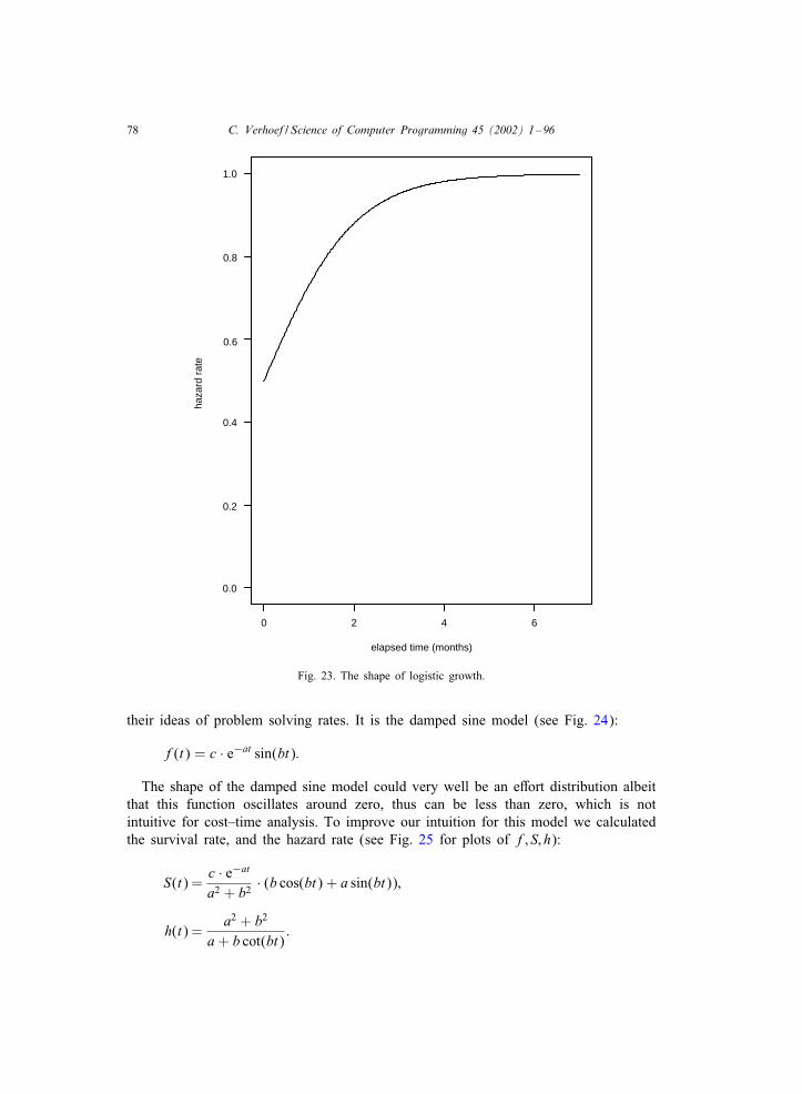
78 C. Verhoef / Science of Computer Programming 45 (2002) 1–96
elapsed time (months)
haza
rd r
ate
0 2 4 6
0.0
0.2
0.4
0.6
0.8
1.0
Fig. 23. The shape of logistic growth.
their ideas of problem solving rates. It is the damped sine model (see Fig. 24):
f(t) = c · e−at sin(bt):
The shape of the damped sine model could very well be an eOort distribution albeitthat this function oscillates around zero, thus can be less than zero, which is notintuitive for cost–time analysis. To improve our intuition for this model we calculatedthe survival rate, and the hazard rate (see Fig. 25 for plots of f; S; h):
S(t) =c · e−at
a2 + b2 · (b cos(bt) + a sin(bt));
h(t) =a2 + b2
a + b cot(bt):
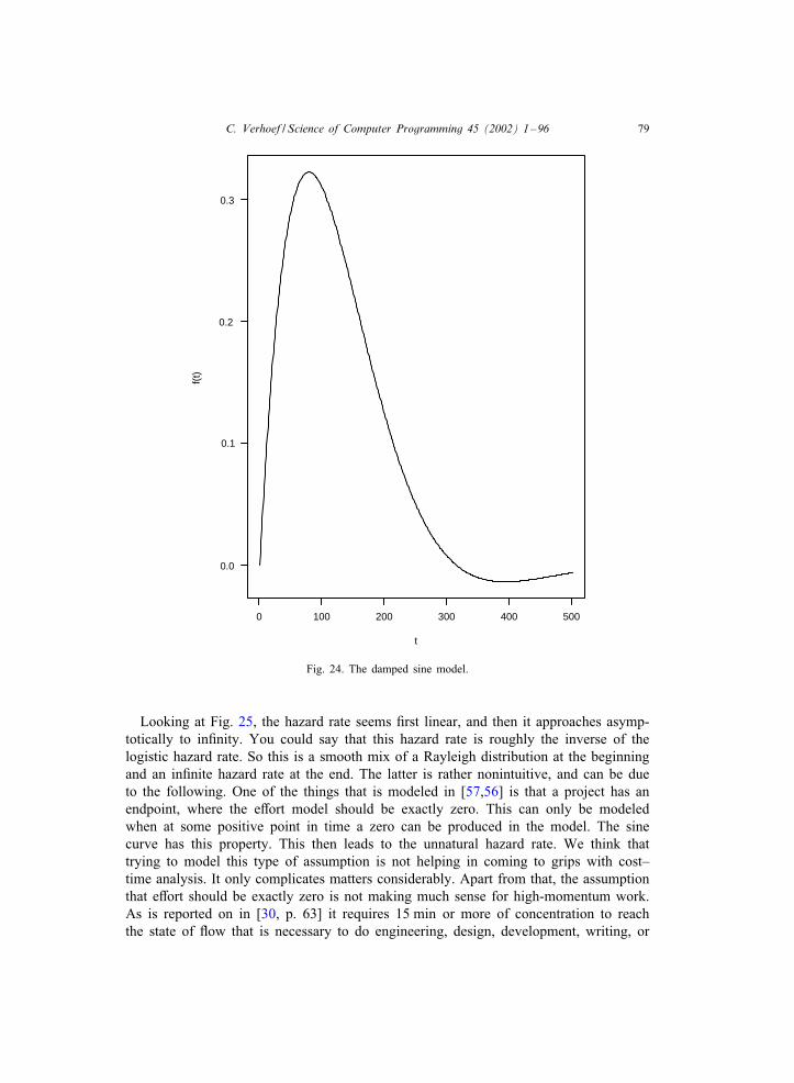
C. Verhoef / Science of Computer Programming 45 (2002) 1–96 79
t
f(t)
0 100 200 300 400 500
0.0
0.1
0.2
0.3
Fig. 24. The damped sine model.
Looking at Fig. 25, the hazard rate seems Crst linear, and then it approaches asymp-totically to inCnity. You could say that this hazard rate is roughly the inverse of thelogistic hazard rate. So this is a smooth mix of a Rayleigh distribution at the beginningand an inCnite hazard rate at the end. The latter is rather nonintuitive, and can be dueto the following. One of the things that is modeled in [57,56] is that a project has anendpoint, where the eOort model should be exactly zero. This can only be modeledwhen at some positive point in time a zero can be produced in the model. The sinecurve has this property. This then leads to the unnatural hazard rate. We think thattrying to model this type of assumption is not helping in coming to grips with cost–time analysis. It only complicates matters considerably. Apart from that, the assumptionthat eOort should be exactly zero is not making much sense for high-momentum work.As is reported on in [30, p. 63] it requires 15 min or more of concentration to reachthe state of Iow that is necessary to do engineering, design, development, writing, or
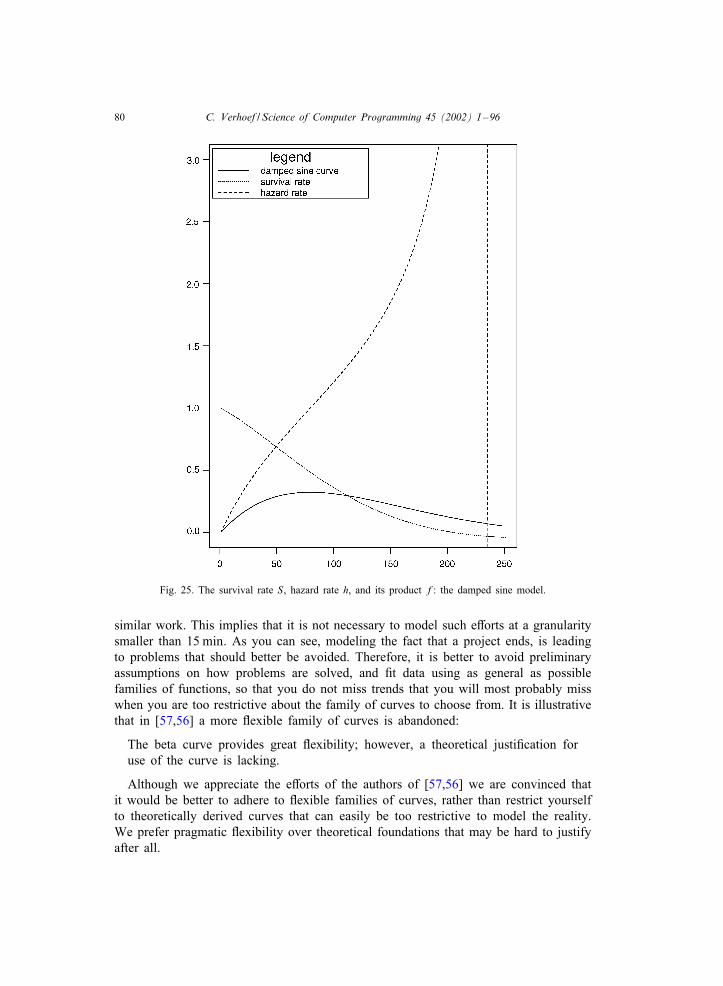
80 C. Verhoef / Science of Computer Programming 45 (2002) 1–96
Fig. 25. The survival rate S, hazard rate h, and its product f: the damped sine model.
similar work. This implies that it is not necessary to model such eOorts at a granularitysmaller than 15 min. As you can see, modeling the fact that a project ends, is leadingto problems that should better be avoided. Therefore, it is better to avoid preliminaryassumptions on how problems are solved, and Ct data using as general as possiblefamilies of functions, so that you do not miss trends that you will most probably misswhen you are too restrictive about the family of curves to choose from. It is illustrativethat in [57,56] a more Iexible family of curves is abandoned:
The beta curve provides great Iexibility; however, a theoretical justiCcation foruse of the curve is lacking.
Although we appreciate the eOorts of the authors of [57,56] we are convinced thatit would be better to adhere to Iexible families of curves, rather than restrict yourselfto theoretically derived curves that can easily be too restrictive to model the reality.We prefer pragmatic Iexibility over theoretical foundations that may be hard to justifyafter all.

C. Verhoef / Science of Computer Programming 45 (2002) 1–96 81
In the next example we will see that a too restrictive model broke down, and that amore Iexible model solved the problems. Moreover, it illustrates the strong relationsbetween lifetime analysis and software cost estimation. Recall the earlier cited US AirForce study by Porter. He used the Weibull distribution for recalibrating the costs andlifetime of R&D programs [97]. Indeed, the linear hazard rate did not give Porterenough freedom to Ct the experimental data to Rayleigh distributions. Apparently, thehazard rate, that he calls performance rate for R&D programs is not linear but followssome diOerent pattern. Without realizing this, he assumes the following hazard rate:�t�−1. Also in Porter’s paper diOerential calculus is used for inference of the cost–timefunction. But again, using the basic concepts of lifetime analysis the probability densityfunction is obvious: �t�−1e−t� . And this is indeed the Weibull distribution that is oftenused in lifetime data analysis.
As another example, recall the learning function in the earlier mentioned textbookby Londeix [78]. In that book, a hazard rate of 2atn is considered. To derive thedistribution, the textbook also uses diOerential calculus. Again, using the lifetime dataanalysis basics, it is trivial to infer the answer.
So you could say that for estimating costs of software projects, R&D programs, andIT portfolio management, the hazard function in lifetime analysis corresponds to theproblem solving rate, that the survival function corresponds to the percent of workremaining, that is, the residual investment, that the distribution function F correspondsto the accumulated cost function, and the density f corresponds to the manpowerbuildup function. Therefore, you can see cost–time analysis as lifetime analysis.
This is in accord with the interpretation of the Rayleigh curve: the linear part standsfor the learning curve to overcome problems one at a time, which is the hazard function,and the quadratic exponential factor represents the velocity with which you can solvethose problems once the solutions are known, which is the survival function.
12.5. Hazard rate and survival function
The hazard and survival function provide central intuitions for a cost–time analysis—just as they justify the use of speciCc models in lifetime analysis. For any cost–timedistribution you can calculate these functions, as we did for a number of known ones, tobetter understand the distribution, and its feasibility. Vice versa, if you know for a factwhat the problem solving rate of an R&D-like project is, then you can immediately inferthe correct distribution. But knowing this rate implies that you presumably understandthe problem in the Crst place, so then it is not an R&D project anymore. This paradoxshows that trying to theoretically infer a cost–time distribution seems to be feasibleonly for well-understood problems. Measuring problem solving rates seems infeasiblefor CMM level 1 organizations, who are lacking an overall metrics program.
To gain insight in the empirically found formula (52) it is therefore worthwhile tocalculate the survival and hazard functions. The survival function is easily inferredfrom formula (53). Formula (54) for quantitative IT portfolio management is
S(t) =�((� + 1)=�; bt�)�((� + 1)=�)
: (54)
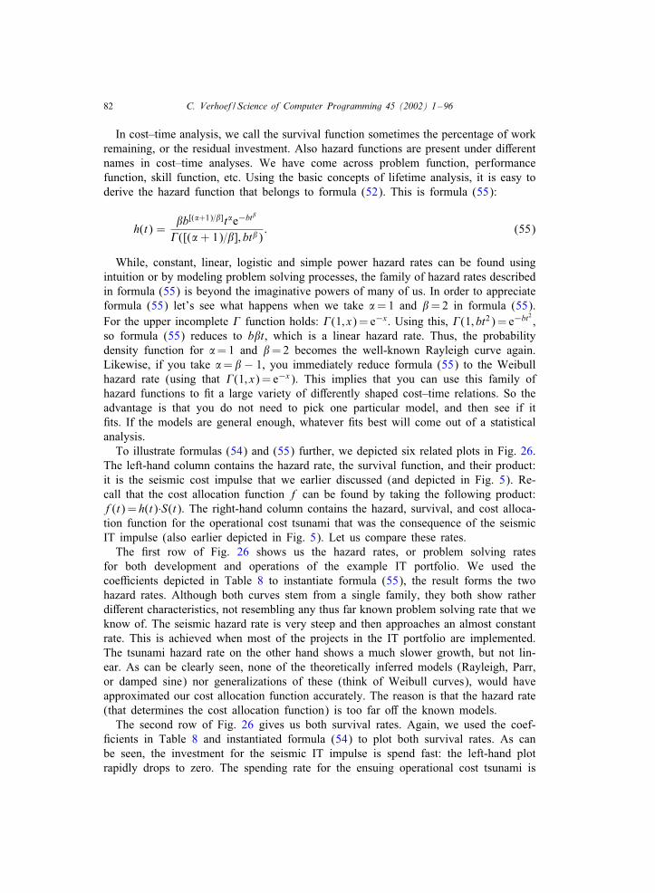
82 C. Verhoef / Science of Computer Programming 45 (2002) 1–96
In cost–time analysis, we call the survival function sometimes the percentage of workremaining, or the residual investment. Also hazard functions are present under diOerentnames in cost–time analyses. We have come across problem function, performancefunction, skill function, etc. Using the basic concepts of lifetime analysis, it is easy toderive the hazard function that belongs to formula (52). This is formula (55):
h(t) =�b[(�+1)=�]t�e−bt�
�([(� + 1)=�]; bt�): (55)
While, constant, linear, logistic and simple power hazard rates can be found usingintuition or by modeling problem solving processes, the family of hazard rates describedin formula (55) is beyond the imaginative powers of many of us. In order to appreciateformula (55) let’s see what happens when we take �= 1 and �= 2 in formula (55).For the upper incomplete � function holds: �(1; x) = e−x. Using this, �(1; bt2) = e−bt2 ,so formula (55) reduces to b�t, which is a linear hazard rate. Thus, the probabilitydensity function for �= 1 and �= 2 becomes the well-known Rayleigh curve again.Likewise, if you take �= � − 1, you immediately reduce formula (55) to the Weibullhazard rate (using that �(1; x) = e−x). This implies that you can use this family ofhazard functions to Ct a large variety of diOerently shaped cost–time relations. So theadvantage is that you do not need to pick one particular model, and then see if itCts. If the models are general enough, whatever Cts best will come out of a statisticalanalysis.
To illustrate formulas (54) and (55) further, we depicted six related plots in Fig. 26.The left-hand column contains the hazard rate, the survival function, and their product:it is the seismic cost impulse that we earlier discussed (and depicted in Fig. 5). Re-call that the cost allocation function f can be found by taking the following product:f(t) = h(t)·S(t). The right-hand column contains the hazard, survival, and cost alloca-tion function for the operational cost tsunami that was the consequence of the seismicIT impulse (also earlier depicted in Fig. 5). Let us compare these rates.
The Crst row of Fig. 26 shows us the hazard rates, or problem solving ratesfor both development and operations of the example IT portfolio. We used thecoeJcients depicted in Table 8 to instantiate formula (55), the result forms the twohazard rates. Although both curves stem from a single family, they both show ratherdiOerent characteristics, not resembling any thus far known problem solving rate that weknow of. The seismic hazard rate is very steep and then approaches an almost constantrate. This is achieved when most of the projects in the IT portfolio are implemented.The tsunami hazard rate on the other hand shows a much slower growth, but not lin-ear. As can be clearly seen, none of the theoretically inferred models (Rayleigh, Parr,or damped sine) nor generalizations of these (think of Weibull curves), would haveapproximated our cost allocation function accurately. The reason is that the hazard rate(that determines the cost allocation function) is too far oO the known models.
The second row of Fig. 26 gives us both survival rates. Again, we used the coef-Ccients in Table 8 and instantiated formula (54) to plot both survival rates. As canbe seen, the investment for the seismic IT impulse is spend fast: the left-hand plotrapidly drops to zero. The spending rate for the ensuing operational cost tsunami is
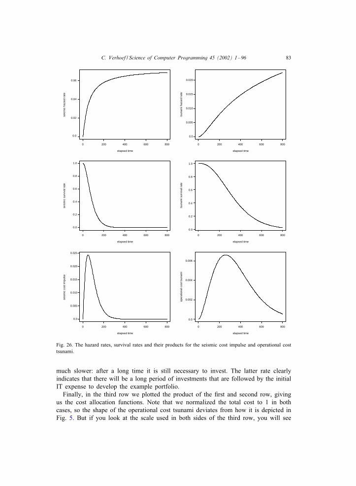
C. Verhoef / Science of Computer Programming 45 (2002) 1–96 83
elapsed time
seis
mic
haz
ard
rate
0 200 400 600 800
0.0
0.02
0.04
0.06
elapsed time
seis
mic
sur
viva
l rat
e
0 200 400 600 800
0.0
0.2
0.4
0.6
0.8
1.0
elapsed time
seis
mic
cos
t im
puls
e
0 200 400 600 800
0.0
0.005
0.010
0.015
0.020
0.025
elapsed time
tsun
ami h
azar
d ra
te
0 200 400 600 800
0.0
0.005
0.010
0.015
0.020
elapsed time
tsun
ami s
urvi
val r
ate
0 200 400 600 800
0.0
0.2
0.4
0.6
0.8
1.0
elapsed time
oper
atio
nal c
ost t
suna
mi
0 200 400 600 800
0.0
0.002
0.004
0.006
Fig. 26. The hazard rates, survival rates and their products for the seismic cost impulse and operational costtsunami.
much slower: after a long time it is still necessary to invest. The latter rate clearlyindicates that there will be a long period of investments that are followed by the initialIT expense to develop the example portfolio.
Finally, in the third row we plotted the product of the Crst and second row, givingus the cost allocation functions. Note that we normalized the total cost to 1 in bothcases, so the shape of the operational cost tsunami deviates from how it is depicted inFig. 5. But if you look at the scale used in both sides of the third row, you will see
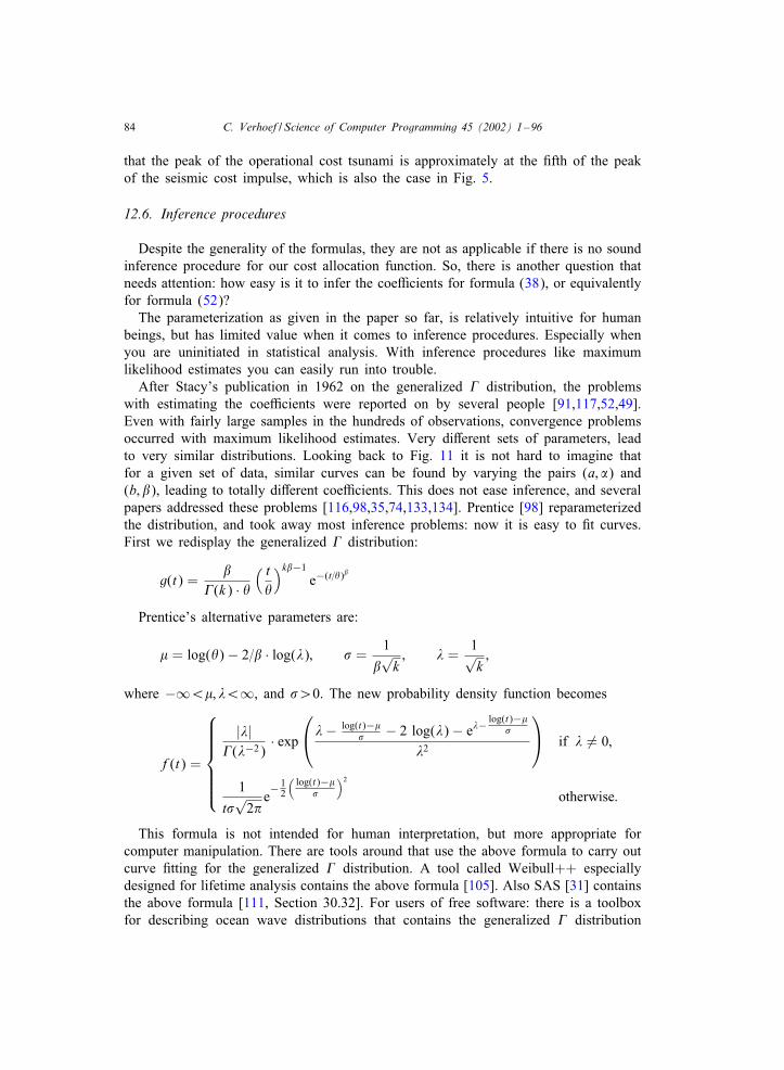
84 C. Verhoef / Science of Computer Programming 45 (2002) 1–96
that the peak of the operational cost tsunami is approximately at the Cfth of the peakof the seismic cost impulse, which is also the case in Fig. 5.
12.6. Inference procedures
Despite the generality of the formulas, they are not as applicable if there is no soundinference procedure for our cost allocation function. So, there is another question thatneeds attention: how easy is it to infer the coeJcients for formula (38), or equivalentlyfor formula (52)?
The parameterization as given in the paper so far, is relatively intuitive for humanbeings, but has limited value when it comes to inference procedures. Especially whenyou are uninitiated in statistical analysis. With inference procedures like maximumlikelihood estimates you can easily run into trouble.
After Stacy’s publication in 1962 on the generalized � distribution, the problemswith estimating the coeJcients were reported on by several people [91,117,52,49].Even with fairly large samples in the hundreds of observations, convergence problemsoccurred with maximum likelihood estimates. Very diOerent sets of parameters, leadto very similar distributions. Looking back to Fig. 11 it is not hard to imagine thatfor a given set of data, similar curves can be found by varying the pairs (a; �) and(b; �), leading to totally diOerent coeJcients. This does not ease inference, and severalpapers addressed these problems [116,98,35,74,133,134]. Prentice [98] reparameterizedthe distribution, and took away most inference problems: now it is easy to Ct curves.First we redisplay the generalized � distribution:
g(t) =�
�(k) · "( t"
)k�−1e−(t=")�
Prentice’s alternative parameters are:
� = log(") − 2=� · log(%); ' =1
�√k; % =
1√k;
where −∞¡�; %¡∞, and '¿0. The new probability density function becomes
f(t) =
|%|�(%−2)
· exp
%− log(t)−�
' − 2 log(%) − e%−log(t)−�
'
%2
if % �= 0;
1
t'√
2)e− 1
2
( log(t)−�'
)2
otherwise:
This formula is not intended for human interpretation, but more appropriate forcomputer manipulation. There are tools around that use the above formula to carry outcurve Ctting for the generalized � distribution. A tool called Weibull++ especiallydesigned for lifetime analysis contains the above formula [105]. Also SAS [31] containsthe above formula [111, Section 30.32]. For users of free software: there is a toolboxfor describing ocean wave distributions that contains the generalized � distribution
C. Verhoef / Science of Computer Programming 45 (2002) 1–96 85
[12]—it is not a coincidence that we associate the long operational cost waves withtsunamis. This is GNU licensed software and the Matlab [80] sources are available,which is handy when you want to tweak the code. Recall that we Ct the curves usingnonlinear regression as implemented in Splus [19,54,129,95]. Indeed, it is not alwaystrivial to Cnd good starting values, and we used techniques similar to [133,134] to Cndthem. Using tools especially geared towards this type of analysis surely improves theease with which you can carry out your own cost–time analysis.
12.7. The generalized F distribution
While many people resort to using restricted families of distributions for softwarecost estimation, this somewhat rigid practice breaks fully down when lifting fromthe project to the portfolio level. One of the reasons is that the projects can be quiteheterogeneous. For instance, the productivity of individual programmers can vary widely.The variation in error detection (or debugging) for small programming eOorts has beenfound to be 26 to 1. Remarkably, the subjects had the same programming experience[110]. These Cndings have been conCrmed in many studies. In another study a 20 to 1ratio of development time for programmers with the same experience [83,29,18,9,128].Usually there will be variation in experience. Comparing low complexity eOorts doneby capable programmers with high complexity eOorts by less capable programmers,can lead to ratio of 1: 400 in productivity diOerences [23, p. 256]. In [23, p. 240] itwas found that for large programming eOorts, this eOect is less pronounced, althoughstill a variation of productivity ratios of 2–4:1 is measured. It will be clear that veryheterogeneous cost–time functions on a per project basis will not be uncommon. Thedecreasing variation is in accord with Markowitz’s work on risk diversiCcation: sincethe variance for productivity has an upper bound, the variance of the total productivityof the entire programming team will approach zero if the team size approaches inCnity[79, p. 107]. And when projects become large, you need more programmers. So forselecting programmers for a team, in theory you could use modern portfolio theory.But given the enormous shortage of programmers, in practice there is not much choice.
Although the generalized � family is fairly general, we like to point out in thissection, that there are even more general distributions, especially designed to deal withheterogeneous data. They are additionally used to test which less general distributionCts the data best. Therefore, we sometimes use another family of distributions thatalso accurately approximates cost–time data for portfolios. This family is more Iexiblethan the generalized � distributions and there are described inference procedures. Thedisadvantage of this family of distributions is that it is relatively unknown outsidethe realm of failure time data analysis. We like to brieIy discuss the generalized Fdistribution as proposed by Prentice [98]. Prentice worked on this subject supported bya grant of a cancer research center [98, p. 614]. The primary use of his distributionwas to incorporate all the known failure time distributions, so that with a test youcould discriminate among them. You could say that he developed mathematical toolsto aim before Cring. In cancer research also heterogeneous populations occur: somewill die, some will be cured, some will not get the disease. We loosely compare thisto the heterogeny of programmer productivity: some are no programmers at all, some
86 C. Verhoef / Science of Computer Programming 45 (2002) 1–96
will never Cnish a program, and some will spread code like a cancerous organism. Thefailure time could be seen as the time it takes to complete the IT development project.
A positive random variable T is said to have a generalized F distribution with � and' as location and scale parameters and s1; s2 as shape parameters, if W = (log T −�)='is the logarithm of a random variable having an F distribution with 2s1 and 2s2 degreesof freedom. The probability density function of W , enhancing formula (52) with respectto Iexibility is
f(w) =(ews1=s2)s1 (1 + ews1=s2)−(s1+s2)
B(s1; s2); (56)
where −∞¡�¡∞, '; s1; s2¿0 and B is the beta function deCned as
B(s1; s2) =�(s1)�(s2)�(s1 + s2)
:
The generalized F distribution contains many other distributions: for '= 1 formula(56) reduces to the F distribution, if si →∞, for i= 1 or 2 formula (56) becomesthe generalized � distribution, if s1 = s2 it reduces to the generalized log-logistic dis-tribution, for s2 = 1 it reduces to the Burr type III, and for s1 = 1 to the Burr typeXII distributions. Burr distributions are used in environmetrics to estimate the con-centrations of chemicals such that a given percentage of species will survive [112].Furthermore, the �, ,2, Poisson, Rayleigh, Log-normal, Log logistic, Pearson type III,Maxwell–Boltzmann and many other distributions are special cases of the generalizedF distribution.
Just as with the generalized � distribution, formula (56) is of limited interest unlessthere are tools and techniques to infer the coeJcients. There is an Splus package toCt both the generalized � and the generalized F distributions. It is called GFCURE,referring to cure rate estimation using the generalized F distribution, and stems fromcancer research [94,93].
12.8. Software cost estimates are censored
In clinical trials it is often desirable to analyze the data before all the individuals havedied. Therefore, it is common to work with so-called censored data. An observation iscensored (or right censored) if the exact value of the observation is not known, but onlythat it is greater than or equal to this observation. For instance, when a software projectis estimated to cost half a million dollar, this can be seen as censored data: it willmost likely be at least $500 000. It seems an established idea in software engineering,that it is not possible to say anything about estimates if the data is censored, that is,no actual data is available [28]. But often, we do have censored data to our avail,especially in IT portfolios, where not only Cnished IT projects, but also projects inprogress, and IT project proposals are present. Finished IT projects provide you withlife and uncensored data, ongoing and proposed ones are characterized by censoreddata. Note that you cannot use censor analysis, if the deviations are arbitrary, thatis, sometimes too much, sometimes accurate, and sometimes too low. There is no
C. Verhoef / Science of Computer Programming 45 (2002) 1–96 87
tradition whatsoever of IT projects being too early, or less costly than anticipated inadvance [58,46–48,42,41,44]. This implies that IT portfolio data is right censored. Bothin lifetime and failure time analysis a lot of research is done to support analysis inthe presence of censored data sets, so we can deploy the results of this work to ouradvantage and analyze IT portfolios more accurately, even in the case where IT projectsare not Cnished. We have not yet applied censor analysis in practice, since for that youneed uncensored data as well. This would imply access to a body of historical data,which is hardly present in CMM level 1 organizations.
12.9. Estimating an empirical survival function
Something that is easily measurable is the spending rate for a set of correlated ITinvestments over time. This is used in cost uncertainty analysis for systems engineering[40] (containing a software component) to capture the cost distribution over time at anearly stage. In that book [40] it is found that in many cases the total cost distribution ofa systems engineering project comprises large numbers of uncorrelated cost items, sotheir accumulation approaches the normal distribution. This assumption enables you toestimate the accumulated cost function at an early stage. As mentioned earlier, empiricalevidence shows that cost allocation functions for R&D projects, software projects, andIT portfolios are not normally distributed. This is shown in [86–88,100–103,97] andby us. So you have to do something diOerent.
If you measure accumulated costs, you equivalently have the residual investment,which is the survival function. In lifetime data analysis, it is also not hard to measurehow the survival of a population over time develops. Techniques are available to esti-mate from these observations the empirical survival function. If you have the survivalfunction, you can infer the hazard rate and the cost allocation function. Product-limitestimates, also known as Kaplan–Meier estimates, are used in lifetime analysis to esti-mate empirical survival functions. Since you do not always want to wait until the entireinvestment is made, your data will be censored. This implies that you need to estimatethe empirical survival function with censored data. For details on these methods werefer the interested reader to [67,75]. If there is enough accounting data, and other ITrelated management data lacks, you can use the residual investment rate to estimate thesurvival function. Also if quantitative IT portfolio management is consolidated withinyour organization, you can track the residual investment rate to check whether thesurvival function that was originally proposed for the IT investment is consistent withthe real spending rate. This type of analysis can then signal at an early stage possibleproblems. In this stage, you are really getting on top of IT.
13. Conclusions
The Clinger Cohen Act of 1996 enforced the use of IT portfolio management but didnot explain how this should be done in operational terms. As far as we know, this paperis the Crst one to describe quantitative IT portfolio management in depth. We hope thatorganizations in general, and in particular, the ones subject to the Clinger Cohen Actwill beneCt from the material presented in this paper. Most organizations are CMM
88 C. Verhoef / Science of Computer Programming 45 (2002) 1–96
level 1 organizations. We argued that CMM level 1 organizations—who need suchtools probably most urgently—can jump start quantitative IT portfolio management bycompensating their lack of historical data with external benchmarks. With examplescomposed from actual quantitative IT portfolio management projects we illustrated ourapproach. Based on our Cndings, we were able to relate our work to an existing body ofknowledge, from which we could borrow methods, insights, techniques, and tools to ouradvantage to solve relevant problems in quantitative IT portfolio management. Com-paring the advancements made in these other areas with the gap in the software Celdwe feel that much work, some of which has been outlined in this paper, is necessaryto nurture and mature quantitative IT portfolio management. When better benchmarksand more historical data becomes available, the numerical values in our formulas willchange, but presumably not their generic form. In our opinion, we developed the Crstiteration of a collection of formulas that form a useful basis for getting started withquantitative IT portfolio management.
Abbreviations
Below we give a lexicographical listing of the used abbreviations plus a brief clar-iCcation. Moreover we refer to formulas, tables, Cgures whenever appropriate. In thelist you will Cnd all but one formula. The exception is the Cxed ratio equation (27)for which no abbreviation was introduced. It is expressing that the operational costallocation per time unit is 20% of the cost allocation per time unit for building thesystem.a: accumulated cost function. This is the integral of formula (38). See formula (39)
for details.adc: accumulated development costs. The formula for adcs calculates the accumulated
development costs, for a given system s over a given time frame. See formula (22).Likewise, the formula for adcP calculates the accumulated development costs for agiven IT portfolio P over a given time frame. See formula (25).aoc: accumulated operational costs. The formula for aocs calculates the accumulated
(minimal) operational costs, for a given system s over a given time frame. See formula(23). Likewise, the formula for aocP calculates the accumulated (minimal) operationalcosts for a given IT portfolio P over a given time frame. See formula (26).atc: accumulated total costs. The formula for atcs calculates the accumulated (min-
imal) total costs, for a given system s over a given time frame. See formula (21).Likewise, the formula for atcP calculates the accumulated (minimal) total costs for agiven IT portfolio P over a given time frame. See formula (24).c: this symbol is overloaded. It stands for an amount of money, that is cost, but it
is also a function name. It is the name we gave to the cost allocation function thatgeneralizes all known cost allocation functions, and that we mainly use to base ourcost–time analyses on. See formula (38) for elaborations.ca: cost allocation. This formula calculates the cost allocation for a system for a
given time. It consists of the operational and development cost allocations (see cadand cao below). See formula (17).
C. Verhoef / Science of Computer Programming 45 (2002) 1–96 89
cad: cost allocation for development. This formula calculates for a given time, thecost allocation that you minimally need to develop a system. Typically you can calcu-late the monthly costs for development. See formula (19).cao: cost allocation of operations. This formula calculates for a given time, the cost
allocation that you minimally need to keep a system operational. You typically use thisformula to calculate monthly operational costs. See formula (20).cc: change in cost. The change in cost equation is the derivative of our proposed
cost allocation equation (which is formula (38)). See formula (40).cco: corporate cost of ownership. This formula gives you for a given IT portfolio
and a given time, the corporate cost that you need to spend to own the portfolio. Seeformula (45).cf: chance on failing projects. There are several related formulas. We have cfi:
the chance on late projects in the information systems industry. See formula (28)for this chance when a given amount of function points is known, and formula (29)if its development time in calendar months is known. We also have cfo, where thesubscript now denotes the outsource industry. Analogously, we have a formula for agiven amount of function points: formula (30), and one if the development time isknown: formula (31).cl: chance on late projects. There are several related formulas. We have cl i: the
chance on late projects in the information systems industry. See formula (32) for thischance when a given amount of function points is known, and formula (33) if its devel-opment time in calendar months is known. We also have clo, where the subscript nowdenotes the outsource industry. Analogously, we have a formula for a given amount offunction points: formula (34), and one if the development time is known: formula (35).d: duration. This symbol is overloaded. First it stands for the duration of a project,
but it is also a function, that returns the duration for development given a deploymenttime of a system in years. See formula (10). When subscripted it stands for the amountof calendar months expressing the amount of calendar months for an information sys-tems project (di) or an outsource development project (do), given its size in functionpoints. See formulas (47) and (50), respectively.dd: development duration. This formula calculates the duration in calendar months
of a development project given its cost. See formula (3). It also calculates the durationin calendar months of a development project given its staO, see formula (7). Finally,it returns the duration of a development project given a known amount of operationalcosts, see formula (12) for that version.df: development fraction. This formula gives you the fraction of the total cost of
ownership that is devoted to development. See formula (15).ead: eOort allocation for development. This is not a generic formula but is a speciCc
formula tailored to an example. We calculated the eOort allocation of an IT projectdescribed in the literature. The formula ead is depicted in Fig. 10.f: this symbol is overloaded. First it stands for a given amount of function points.
But is also a function. It is the probability distribution function f(t) that belongs toour proposed cost allocation function (deCned in formula (38)). See formula (52). Italso stands for the probability density function known as the generalized F distribution,as stated in formula (56).
90 C. Verhoef / Science of Computer Programming 45 (2002) 1–96
F : this is the cumulative distribution function belonging to function f. See formula(53) for details.fe: failure exposure. This formula accumulates the failure chances of all the individual
projects in a portfolio. All you need to know are the (estimated) durations of all theprojects in the portfolio. See formula (36).h: hazard rate. Formula (55) is the hazard rate that belongs to the probability density
function that we deCned in formula (38).le: late exposure. This formula accumulates the chances of all the individual projects
in a portfolio on being late. All you need to know are the (estimated) durations of allthe projects in the portfolio. See formula (37).mco: minimal cost of operation. This formula predicts the minimal cost to keep a
system running given its development duration. See formula (11).md: maintenance duration. This formula calculates the maintenance duration for a
given cost. See formula (4). It also calculates the maintenance duration for a givenstaO size, see formula (8).mrt: minimal ROI threshold. This is not a generic formula but is a speciCc formula
that calculates minimal ROI threshold of an IT investment example. This example issummarized in Table 4. The mrt formula is depicted in Fig. 7.mtco: minimal total cost of ownership. This formula calculates for a given devel-
opment duration the minimal total cost of ownership over the entire life-cycle of thesystem. Minimal means here without functional changes. See formula (13).nsd: number of staO for development. This formula calculates for a given duration
of a development project, the number of staO needed. See formula (5).nsm: number of staO for maintenance. This formula calculates for a given duration
of a maintenance project, the number of staO needed. See formula (6).of: operational fraction. This formula gives you the fraction of the total cost of
ownership that is devoted to maintenance. See formula (16).p: productivity. We have several formulas for diOerent industries. We have pi giving
the productivity for developing information systems in function points per staO monthfor a given amount of function points. See formula (46). Analogously, formula (49)returns for a given amount of function points the productivity of outsourcers in functionpoints per staO month.pt: peak time. With formula (41) we can calculate the time when the peak cost
needs to be allocated to a portfolio that satisCes a cost allocation function with theshape of formula (38).pc: peak cost. This formula calculates the peak cost for a given cost allocation
function of the shape proposed by formula (38). See formula (42).r: the ratio of minimal cost of operation to development cost. See formula (14).rs: retirement of system s. This formula is the absolute-time variant of formula (9):
given an initiation time and a delivery time, it calculates the retirement time for agiven system. See formula (18).rf: repayment factor. This formula calculates for a given cost allocation function of
the shape as proposed by formula (38), and a given time, the amount of money thatyou still have to invest to develop and operate the portfolio described by the givencost allocation function. See formula (44).

C. Verhoef / Science of Computer Programming 45 (2002) 1–96 91
S: survival function. Formula (54) is the survival function that belongs to the prob-ability density function (52) that we derived from our cost allocation function (38).tcd: total cost of development. We have several of these. First there is a formula,
that for a given development time calculates the cost. See formula (1). Then thereare several formulas that are based on function points, and diversiCed to industry. Wehave tcd i that for a given amount of function points gives the development costs of aninformation systems project, see formula (48). Analogously, we have tcdo that returnsfor a given amount of function points, the development costs of a project done byoutsourcers, see formula (51) for details.tcm: total cost of maintenance. This formula calculates the total cost of a maintenance
project for a given duration. See formula (2).tco: total cost of ownership. This formula calculates the total cost of ownership for
an IT portfolio that is described by an instantiation of formula (38). See formula (43).y(d): years that a system is in its deployment phase. With formula (9) we can
calculate for a given development time, the number of calendar years that a system isin deployment.
Acknowledgements
This paper is the result of many fruitful interactions with people from industryto whom we are indebted. In particular, we would like to express our gratitude toDr John F.A. Spangenberg (Head of IT Performance and Investment Managementat ING Group 4) for his encouragement to report on our work on quantitative ITportfolio management. We thank ING Group for underscoring the relevance of ourresearch on quantitative IT portfolio management by a partial sponsorship. Furthermore,we thank David Faust (Director, Core Services – Global Equities Technology andOperations, Deutsche Bank AG) for his valuable comments, discussions and suggestionsfor improvements. We thank Hans van Vliet (VU, Amsterdam) for useful commentson the penultimate version of this paper.
References
[1] A.J. Albrecht, Measuring application development productivity, in the Proc. Joint SHARE/GUIDE/IBMApplication Development Symp., 1979, pp. 83–92.
[2] L. Amoroso, Ricerche intorno alla curva dei redditi, Ann. Mat. Pura Appl. 21 (4) (1932) 123–159.[3] J. Asundi, R. Kazman, A Foundation for the Economic Analysis of Software Architectures, in:
K. Sullivan (Ed.), Proc. 3rd Workshop on Economics-Driven Software Engineering Research(EDSER-3), 2001. Available via: www.cs.virginia.edu/∼sullivan/edser3/asundi.pdf.
[4] L.J. Bain, Analysis for the linear failure rate distribution, Technometrics 16 (1974) 551–559.[5] S. Berinato, Do the MATH, CIO Mag. (2001). Available via: www.cio.com/archive/100101/
math.html.[6] B. Boehm, Software Engineering Economics, Prentice-Hall, Englewood CliOs, NJ, 1981.
4 ING Group is a global player in the Cnancial services and insurance industry, investing approximately2.5 billion Euro per annum on information technology.
92 C. Verhoef / Science of Computer Programming 45 (2002) 1–96
[7] B.W. Boehm, The high cost of software, in: E. Horowitz (Ed.), Practical Strategies for DevelopingLarge Software Systems, Addison-Wesley, Reading, MA, USA, 1975.
[8] B.W. Boehm, Software engineering, IEEE Trans. Comput. C-25 (1976) 1226–1241.[9] B.W. Boehm, P.N. Papaccio, Understanding and controlling software costs, IEEE Trans. Software Eng.
SE-14 (10) (1988) 1462–1477.[10] J. Bosch, Design and Use of Software Architectures—Adopting and Evolving a Product-Line Approach,
Addison-Wesley, Reading, MA, 2000.[11] K. BrZannZas, N. Nordman, Conditional skewness modelling for stock returns, Technical Report 562,
Department of Economics, Ume[a University, 2001.[12] P.A. Brodtkorb, P. Johannesson, G. Lindgren, I. Rychlik, J. Ryd\en, E. SjZo, WAFO—a Matlab toolbox
for analysis of random waves and loads, in the Proc. 10th International OOshore and Polar EngineeringConf., 2000, pp. 343–350.
[13] F.P. Brooks Jr., The Mythical Man-Month—Essays on Software Engineering, Anniversary Edition,Addison-Wesley, Reading, MA, 1995.
[14] W.K. Brown, K.H. Wohletz, Derivation of the Weibull distribution based on physical principlesand its connection to the Rosin–Rammler and lognormal distributions, J. Appl. Phys. 78 (4) (1995)2758–2763.
[15] J. Brunekreef, B. Diertens, Towards a user-controlled software renovation factory, in: P. Nesi,C. Verhoef (Eds.), Proc. Third European Conf. on Maintenance and Reengineering, IEEE ComputerSociety Press, Rockville, MD, 1999, pp. 83–90.
[16] S. Butler, P. Chalasani, S. Jha, O. Raz, M. Shaw, The potential of portfolio theory in guidingsoftware decisions, in: K. Sullivan (Ed.), Proc. 1st Workshop on Economics-Driven SoftwareEngineering Research (EDSER-1), 1999. Available via: www.cs.virginia.edu/∼sullivan/EDSER-1/PositionPapers/jha.pdf.
[17] S. Butler, S. Jha, M. Shaw, When good models meet bad data—applying quantitativeeconomic models to qualitative engineering judgements, in: K. Sullivan (Ed.), Proc. 2ndWorkshop on Economics-Driven Software Engineering Research (EDSER-2), 2000. Available via:http://www.cs.virginia.edu/∼sullivan/edser2/shaw.pdf.
[18] D. Card, A software technology evaluation program, Inform. Software Technol. 29 (6) (1987)291–300.
[19] J.M. Chambers, T.J. Hastie (Eds.), Statistical Models in S. Wadsworth & Brooks/Cole, PaciCc Grove,CA, 1992.
[20] E.J. Chikofsky, J.H. Cross, Reverse engineering and design recovery: a taxonomy, IEEE Software7 (1) (1990) 13–17.
[21] C. Cifuentes, K.J. Gough, Decompilation of binary programs, Software—Practice Exper. 25 (7) (1995)811–829.
[22] P. Clements, L.M. Northrop, Software Product Lines—Practices and Patterns, Addison-Wesley,Reading, MA, 2002.
[23] S.D. Conte, H.E. Dunsmore, V.Y. Shen, Software Engineering Metrics and Models, TheBenjamin/Cumming Publishing Company, Inc., Menlo Park, CA, 1986.
[24] Federal CIO Council, A summary of Crst practices and lessons learned in information technologyportfolio management, Technical Report, Federal CIO Council, Best Practices Committee, 2002.Available via: http://cio.gov/Documents/BPC Portfolio final.pdf.
[25] R. D’Addario, Intorno alla curva dei redditi di Amoroso, Riv. Italiana Statist. Econ. Fnanza, anno 4(1) (1932).
[26] E.B. Daly, Management of software engineering, IEEE Trans. Software Eng. SE-3 (3) (1977)229–242.
[27] S.M. Dekleva, The inIuence of the information systems development approach on maintenance, MISQuart. 16 (3) (1992) 355–372.
[28] T. DeMarco, Controlling Software Projects–Management Measurement & Estimation, Yourdon PressComputing Series, Englewood CliOs, NJ, 1982.
[29] T. DeMarco, T. Lister, Programmer performance and the eOects of the workplace, in: Proc. 8thInternat. Conf. on Software Engineering, ICSE-8, IEEE Computer Society, Silver Spring, MD, 1985,pp. 268–272.
C. Verhoef / Science of Computer Programming 45 (2002) 1–96 93
[30] T. DeMarco, T. Lister, Peopleware—Productive Projects and Teams, Dorset House, New York, NY,1987.
[31] G. Der, B.S. Everitt, Handbook of Statistical Analyses Using SAS, CRC Press, Boca Raton, FL, 2001.[32] J. Doe, C. Verhoef, Software Product Line Migration and Deployment, 2002, unpublished manuscript.
(J. Doe is at the moment of publication still an anonymous author.)[33] J.B. Dreger, Function Point Analysis, Prentice-Hall, Englewood CliOs, NJ, 1989.[34] J.L. ElshoO, An analysis of some commercial PL/I programs, IEEE Trans. Software Eng. SE-2 (2)
(1976) 113–120.[35] V.T. Farewell, R.L. Prentice, A study of distributional shape in life testing, Technometrics 19 (1977)
69–75.[36] J. Feiman, N. Frey, Migrating legacy developers to Java: costs, risks and strategies, Technical Report,
GartnerGroup, Stamford, CT, USA, 2001.[37] L.G. Freeman, C. Cifuentes, An industry perspective on decompilation, in: H. Yang, L. White (Eds.),
Internat. Conf. on Software Maintenance, 1999, Printed in the short paper appendix.[38] H.L. Gantt, Organizing for Work, Harcourt, Brace & Howe, New York, 1919.[39] D. Garmus, D. Herron, Function Point Analysis—Measurement Practices for Successful Software
Projects, Addison-Wesley, Reading, MA, 2001.[40] P.R. Garvey, Probability Methods for Cost Uncertainty Analysis—A Systems Engineering Perspective,
Marcel Dekker Inc., New York, 2000.[41] R.L. Glass, Computing Calamities—Lessons Learned From Products, Projects, and Companies that
Failed, Prentice-Hall, Englewood CliOs, NJ, 1998.[42] R.L. Glass, Software Runaways—Lessons Learned from Massive Software Project Failures,
Prentice-Hall, Englewood CliOs, NJ, 1998.[43] R.L. Glass, A new answer to how important is mathematics to the software practitioner? IEEE Software
17 (6) (2000) 135–136.[44] R.L. Glass, ComputingFailure.com—War Stories from the Electronic Revolution, Prentice-Hall,
Englewood CliOs, NJ, 2001.[45] United States Government, Clinger Cohen Act of 1996 and Related Documents, 1996. Available via:
www.c3i.osd.mil/org/cio/doc/CCA-Book-Final.pdf.[46] The Standish Group, CHAOS, 1995. Retrievable via: standishgroup.com/visitor/chaos.htm (Current
February 2001).[47] The Standish Group, CHAOS: A Recipe for Success, 1999. Retrievable via: www.pm2go.com/
sample research/chaos1998.pdf.[48] The Standish Group, EXTREME CHAOS, 2001. Purchase via: https://secure.standishgroup.
com/reports/reports.php.[49] H.W. Hager, L.J. Bain, Inferential procedures for the generalized gamma distribution, J. Amer. Statist.
Assoc. 65 (1970) 1601–1609.[50] B. Hall, Year 2000 tools and services, in: Symp./ITxpo 96, The IT Revolution Continues: Managing
Diversity in the 21st century. GartnerGroup, 1996.[51] M. Hanna, Maintenance burden begging for a remedy, Datamation, April 1993, pp. 53–63.[52] H.L. Harter, Maximum-likelihood estimation of the parameters of a four-parameter generalized gamma
population for complete and censored samples, Technometrics 9 (1967) 159–165.[53] G. Hector, Breaking the Bank—the Decline of BankAmerica, Little, Brown & Company, Boston, MA,
1988.[54] S. Huet, M.-A. Gruet, Stastical Tools for Nonlinear Regression—A Practical Guide with S-Plus
Examples, Springer, Berlin, 1996.[55] IBM Corporation, Transaction Processing Facility—General Information, 4.1 Edition, 1993. Available
via: www-3.ibm.com/software/ts/tpf/images/gtpgim00.pdf.[56] W. Jarvis, New approaches to phasing of resources, in the Proc. 34th Annual Department
of Defense Cost Analysis Symp. 2001. Available via: www.ra.pae.osd.mil/adodcas/Presentations%202001/RSCAllocation.PDF.
[57] W. Jarvis, E. Pohl, Program execution eJciency and resource phasing, in the Proc. 32ndAnnual Department of Defense Cost Analysis Symp., 1999. Available via: www.ra.pae.osd.mil/adodcas/slides/jarvis33.pdf.
94 C. Verhoef / Science of Computer Programming 45 (2002) 1–96
[58] J. Johnson, Chaos: the dollar drain of IT project failures, Appl. Dev. Trends 2 (1) (1995) 41–47.[59] C. Jones, Programming Productivity, McGraw-Hill, New York, 1986.[60] C. Jones, Assessment and Control of Software Risks, Prentice-Hall, Englewood CliOs, NJ, 1994.[61] C. Jones, Applied Software Measurement: Assuring Productivity and Quality, 2nd Edition,
McGraw-Hill, New York, 1996.[62] C. Jones, Patterns of Software Systems Failure and Success, International Thomsom Computer Press,
Boston, MA, 1996.[63] C. Jones, Estimating Software Costs, McGraw-Hill, New York, 1998.[64] C. Jones, The Year 2000 Software Problem—Quantifying the Costs and Assessing the Consequences,
Addison-Wesley, Reading, MA, 1998.[65] C. Jones, Software Assessments, Benchmarks, and Best Practices, Information Technology Series,
Addison-Wesley, Reading, MA, 2000.[66] N. Jones, Year 2000 market overview, Technical Report, GartnerGroup, Stamford, CT, USA, 1998.[67] J.D. KalbIeisch, R.L. Prentice, The Statistical Analysis of Failure Time Data, Wiley, New York, 1980.[68] C.F. Kemerer, Reliability of function points measurement—a Celd experiment, Comm. ACM 36 (2)
(1993) 85–97.[69] C.F. Kemerer, B.S. Porter, Improving the reliability of function point measurement: an empirical study,
IEEE Trans. Software Eng. SE-18 (11) (1992) 1011–1024.[70] T.A. Kirkpatrick, Research: CIOs speak on ROI, CIO Insight, 1(11) (2002). Available via:
www.cioinsight.com, results of questionnaire available via: common.ziffdavisinternet.com/download/0/1396/0110 rio research.pdf.
[71] D. Kodlin, A new response time distribution, Biometrics 23 (1967) 227–239.[72] A. Krause, M. Olson, Basics of S and S-Plus, 2nd Edition, Springer, Berlin, 2000.[73] L. Lamport, How to Tell a Program from an Automobile, in: J. Tromp (Ed.), A Dynamic
and Quick Intellect—Liber Amicorum in honor of Paul Vitanyi’s 25-year jubilee, CWI, 1996,pp. 77–79. Available via: research.microsoft.com/users/lamport/pubs/automobile.pdf.
[74] J.F. Lawless, Inference in the generalized gamma and log gamma distributions, Technometrics 22(1980) 409–419.
[75] J.F. Lawless, Statistical Models and Methods for Lifetime Data, Wiley, New York, 1982.[76] T.C. Lethbridge, Priorities for the education and training of software engineers, J. Systems Software
53 (1) (2000) 53–71.[77] B.P. Lientz, E.B. Swanson, Software Maintenance Management—A Study of the Maintenance of
Computer Application Software in 487 Data Processing Organizations, Addison-Wesley, Reading, MA,1980.
[78] B. Londeix, Cost Estimation for Software Development, Addison-Wesley, Reading, MA, 1987.[79] H.M. Markowitz, Portfolio Selection—EJcient DiversiCcation of Investments, Cowles Foundation For
Research in Economics and Yale University, vol. 16, Wiley, New York, 1967 (3rd printing).[80] W.L. Martinez, A.R. Martinez, Computational Statistics Handbook with MATLAB, CRC Press, Boca
Raton, FL, 2001.[81] S. McConnell, Rapid Development, Microsoft Press, Redmond, WA, 1996.[82] F.W. McFarlan, Portfolio approach to information systems, Harvard Business Rev. 59 (5) (1981)
142–150.[83] H. Mills, Software Productivity, Little Brown, 1983.[84] S.N. Mohanty, Software cost estimation: present and future, Software—Practice Exper. 11 (1981)
103–121.[85] M. Mustatevic, Automation of function point counting, Master’s Thesis, University of Amsterdam,
Programming Research Group, 2000 (in Dutch).[86] P.V. Norden, Curve Ctting for a model of applied research and development scheduling, IBM J. Res.
Dev. 2 (3) (1958).[87] P.V. Norden. Useful tools for project management, in: B.V. Dean (Ed.), Operations Research in
Research and Development Wiley, New York, 1963.[88] P.V. Norden, Useful tools for project management, in: M.K. Starr (Ed.), Management of Production,
Penguin Books, 1970, pp. 71–101.
C. Verhoef / Science of Computer Programming 45 (2002) 1–96 95
[89] United States General Accounting OJce, Information Technology Investment Management—A Frame-work for Assessing and Improving Process Maturity, 2000. Available via: www.gao.gov/special.pubs/10 1 23.pdf.
[90] F.N. Parr, An alternative to the Rayleigh curve model for software development eOort, IEEE Trans.Software Eng. SE-6 (3) (1980) 291–296.
[91] V.B. Parr, J.T. Webster, A method for discriminating between failure density functions used inreliability predictions, Technometrics 7 (1965) 1–10.
[92] M.C. Paulk, C.V. Weber, B. Curtis, M.B. Chrissis, The Capability Maturity Model: Guidelines forImproving the Software Process, Addison-Wesley Publishing Company, Reading, MA, 1995.
[93] P.Y. Peng, GFCURE—An S-PLUS Package for Parametric Analysis of Survival Data with a PossibleCured Fraction, 1999. Available via: www.math.mun.ca/∼ypeng/research/gfcure/.
[94] Y. Peng, K.B.G. Dear, J.W. Denham, A generalized F mixture model for cure rate estimation, Statist.Med. 17 (1998) 813–830.
[95] J.C. Pinheiro, D.M. Bates, Mixed-EOects Models in S and S-PLUS, Springer, Berlin, 2000.[96] M.E. Porter, Competitive Strategy—Techniques for Analyzing Industries and Competitors, The Free
Press, New York, 1980.[97] P.H. Porter, Revising R&D program budgets when considering funding curtailment with a Weibull
Model, Master’s Thesis, Air University, Air Force Institute of Technology, Wright-Patterson Air ForceBase, Ohio, USA, March 2001.
[98] R.L. Prentice, A log gamma model and its maximum likelihood estimation, Biometrika 61 (1974)539–544.
[99] R.L. Prentice, Discrimination among some parametric models, Biometrika 62 (3) (1975) 607–614.[100] L.H. Putnam, A macro-estimation methodology for software development, in the Proc. IEEE
COMPCON 76 Fall, IEEE Computer Society Press, Silver Spring, MD, 1976, pp. 138–143.[101] L.H. Putnam, A general empirical solution to the macro software sizing and estimating problem, IEEE
Trans. Software Eng. SE-4 (4) (1978) 345–361.[102] L.H. Putnam, W. Myers, Measures for Excellence—Reliable Software on Time, Within Budget,
Yourdon Press Computing Series, 1992.[103] L.H. Putnam, R.W. Wolverton, Quantitative management: Software cost estimating, in the Proc. IEEE
Computer Society First Computer Software and Applications Conf. (COMPSAC 77), IEEE ComputerSociety Press, Silver Spring, MD, 1977, pp. 8–11.
[104] A.W. Rathe (Ed.), Gantt on Management: Guidelines for Today’s Executive, American ManagementAssociation, New York, 1961.
[105] ReliaSoft Corporation, Life Data Analysis Reference, rev. 2001 Edition, 2001. www.weibull.com/lifedatawebcontents.htm.
[106] J. Reutter, Maintenance is a management problem and a programmer’s opportunity, in: A. Orden,M. Evens (Eds.), 1981 National Computer Conf., AFIPS Conf. Proc., vol. 50, AFIPS Press, Arlington,VA, 1981, pp. 343–347.
[107] P. Rosin, E. Rammler, The laws governing the Cneness of powdered coal, J. Inst. Fuel 7 (31) (1933)29–36.
[108] H. Rubin, Worldwide Benchmark Report for 1997, Pound Ridge, NY; Rubin Systems, Inc., 1997.[109] H. Rubin, M. Johnson, What’s going on in IT?—summary of results from the worldwide
IT trends and benchmark report, 2002, Technical Report, Metagroup, 2002. Available via:metricnet.com/pdf/whatIT.pdf.
[110] H.W. Sackman, W.J. Erikson, E.E. Grant, Exploratory experimental studies comparing online ando]ine programming performance, Comm. ACM 11 (1) (1968) 3–11.
[111] SAS Institute Inc., SAS/QC User’s Guide, Version 8, 8.2 Edition, 2000.[112] Q. Shao, Estimation for hazardous concentrations based on NOEC toxicity data: an alternative approach,
Environmetrics 11 (5) (2000) 583–595.[113] H.M. Sneed, C. Verhoef, Business process reengineering, in: J.J. Marciniak (Ed.), Encyclopedia of
Software Engineering, 2nd Edition, Wiley, New York, 2001, pp. 83–95.[114] SPSS. SPSS 10.0 Syntax Reference Guide, 1st Edition, Prentice-Hall PTR, Englewood CliOs, NJ, 1999.[115] E.W. Stacy, A generalization of the gamma distribution, Ann. Math. Statist. 33 (3) (1962) 1187–1192.
96 C. Verhoef / Science of Computer Programming 45 (2002) 1–96
[116] E.W. Stacy, Quasimaximum likelihood estimators for two-parameter gamma distributions, IBM J. Res.Dev. 17 (1973) 115–124.
[117] E.W. Stacy, G.A. Mihram, Parameter estimation for a generalized gamma distribution, Technometrics7 (1965) 349–358.
[118] T.D. Steiner, D.B. Teixeira, Technology in Banking—Creating Value and Destroying ProCts,Irwin/McGraw-Hill, New York, 1990.
[119] P.A. Strassmann, Information PayoO—The Transformation of Work in the Electronic Age, TheInformation Economics Press, New Canaan, Connecticut, USA, 1985.
[120] P.A. Strassmann, The Business Value of Computers—An Executive’s Guide, The InformationEconomics Press, New Canaan, Connecticut, USA, 1990.
[121] P.A. Strassmann, The policies and realities of CIM—lessons learned, in the Proc. 4th Armed ForcesCommunications and Electronics Association Conf., AFCEA, Fairfax, VA, USA, 1993, pp. 1–19.
[122] P.A. Strassmann, The Politics of Information Management—Policy Guidelines, The InformationEconomics Press, New Canaan, Connecticut, USA, 1995.
[123] P.A. Strassmann, The Squandered Computer—Evaluating the Business Alignment of InformationTechnologies, The Information Economics Press, New Canaan, Connecticut, USA, 1997.
[124] P.A. Strassmann, Information Productivity—Assessing the Information Management Costs of USIndustrial Corporations, The Information Economics Press, New Canaan, Connecticut, USA, 1999.
[125] P. Tate, The big spenders, Information Strategy, December–January 1998–1999, pp. 30–37.[126] A.A. Terekhov, C. Verhoef, The realities of language conversions, IEEE Software 17(6) (2000)
111–124. Available at http://http://www.cs.vu.nl/∼x/cnv/s6.pdf.[127] W.L. Trainor, Software: from satan to saviour, in the Proc. National Aerospace and Electronics Conf.,
1973.[128] J. Valett, F.E. McGarry, A summary of software measurement experiences in the software engineering
laboratory, J. Systems Software 9 (2) (1989) 137–148.[129] W.N. Venables, B.D. Ripley, Modern Applied Statistics with S-PLUS, 3rd Edition, Springer, Berlin,
1999.[130] C. Verhoef, Towards automated modiCcation of legacy assets, Ann. Software Eng. 9 (2000) 315–336.
Available at http://www.cs.vu.nl/∼x/ase/ase.html.[131] W. Weibull, A statistical theory of the strength of materials, in: Proc. No. 151. The Royal Swedish
Institute of Engineering Research, Stockholm, 1939.[132] S. Wolfram, Mathematica Book, 4th Edition, Cambridge University Press, Cambridge, 1999.[133] J.Y. Wong, Simultaneously estimating the three parameters of the generalized gamma distribution,
Microelectron. Reliability 33 (15) (1993) 2225–2232.[134] J.Y. Wong, Simultaneously estimating with ease the three parameters of the generalized gamma
distribution, Microelectron. Reliability 33 (15) (1993) 2233–2242.[135] F. Wright, Computing with MAPLE, Chapman & Hall/CRC, London, 2001.[136] E. Yourdon, Death March—The Complete Software Developer’s Guide to Surviving ‘Mission
Impossible’ Projects, Prentice-Hall, Englewood CliOs, NJ, 1997.