Clemson UniversityTigerPrints

All Theses Theses

7-2008

QUANTITATIVE MODELING OF SOILPROPERTIES BASED ON COMPOSITIONAND APPLICATION TO DYNAMIC TIRETESTINGSumalatha YaskiClemson University, syaski@clemson.edu

Follow this and additional works at: https://tigerprints.clemson.edu/all_theses

Part of the Engineering Mechanics Commons

This Thesis is brought to you for free and open access by the Theses at TigerPrints. It has been accepted for inclusion in All Theses by an authorizedadministrator of TigerPrints. For more information, please contact kokeefe@clemson.edu.

Recommended CitationYaski, Sumalatha, "QUANTITATIVE MODELING OF SOIL PROPERTIES BASED ON COMPOSITION AND APPLICATIONTO DYNAMIC TIRE TESTING" (2008). All Theses. 433.https://tigerprints.clemson.edu/all_theses/433

i

QUANTITATIVE MODELING OF SOIL PROPERTIES BASED

ON COMPOSITION AND APPLICATION

TO DYNAMIC TIRE TESTING

A Thesis

Presented to

the Graduate School of

Clemson University

In Partial Fulfillment

of the Requirements for the Degree

Master of Science

Mechanical Engineering

by

Sumalatha Yaski

August 2008

Accepted by:

Laine M. Mears, Committee Chair

Joshua D. Summers

Lawrence W. Grimes

ii

ABSTRACT

A new dimension of success in automotive supply is time-based competition. This

especially comes to light in tire development, with companies striving to enhance the

testing methodologies for reduction in development time. Modeling and development of

off-road tires is particularly difficult due to a lack of quantitative descriptions of the

operating environment for model validation. Off-road tire evaluation is subjective,

expensive, site dependent, and testing of such tires is typically carried out under lower

levels of control. The objective of this work is to create fundamental descriptions of

pertinent composition based soil properties and to directly relate these properties to

evaluate the tire performance. A major contribution of this research is to provide a

quantitative measure of soil properties especially with respect to adhesion and plastic

behavior. Two models are developed: one for soil strength and the other for adhesion,

which are used to study the behavior of wet soil in a deformable channel.

For experimental testing, Geotechnical Engineering methods such as Sieve

Analysis, Hydrometer Analysis, and Atterberg Limits Analysis are adapted on a smaller

scale to evaluate fundamental soil properties such as texture, grain size distribution,

composition and plasticity. Classical materials method such as compression testing is

adapted in soil strength evaluation. Certain composition based properties for which no

standard test exist, new testing methodologies are developed and prototyped.

The newly developed methodologies that are used to define the non-existing

properties helped in validating the physics-based models. Statistical evaluation technique

iii

of multivariable regression is employed to find the best fit model applicable to a broad

range of soil compositions.

These soil models can be combined with existing tire behavior models to better

predict new off-road tire design performance, thus reducing prototype evaluation

iterations, overall development time and development cost. An additional benefit of the

new methodologies is the ability to quantitatively evaluate rapidly-manufactured tire

tread samples rather than requiring full prototype production.

iv

DEDICATION

I dedicate this work to the memory of my grandmother, late Mrs. Susheela Bai

and my family without whose support this work would not have been possible.

v

ACKNOWLEDGMENTS

A thesis work of this magnitude is not possible without the help of several people

directly or indirectly. It is with immense satisfaction that I present this practical

experience in the form of a thesis report carried out in Clemson University.

I would like to express my sincere and profound gratitude to my advisor Dr. Laine

M. Mears for extending his continuous support and encouragement throughout this

research. With his immense knowledge and intellect, Dr. Mears helped me in focusing

and developing new ideas which made my research easy. I am grateful to him for

motivating me to take up this project and for the successful complete of it.

I would also like to thank the other committee members Dr. Joshua Summers and

Dr. Larry Grimes for helping me with their valuable advices. Dr. Summers‟s feedback

helped me in making my work take a better shape and achieve the goals of the research.

I take this opportunity to thank Dr. Jonathan Maier, Dr. Virgil Quisenberry, Dr.

Michael Vatalaro, and Dr. Ronald Andrus for their valuable advices.

I would like to thank Matt Schuster, Arpita Biswas, Siva Chavali, Kameswara R

Nara, Vamshi Goli, Pavan Seemakurty, Swathi Chimalapati, Souharda Raghavendra for

their timely help, support and encouragement during the tough times of the project.

Last but not the least, I would like to thank Michelin for providing me an

opportunity to work on a very good project. I am very much indebted to Mr. Pat Buresh

and Mr. Phil Berger who created the ground work for this project and whose timely

suggestions and cooperation helped me to overcome difficult times.

vi

TABLE OF CONTENTS

TITLE .................................................................................................................................. i

ABSTRACT ........................................................................................................................ ii

DEDICATION ................................................................................................................... iv

ACKNOWLEDGMENTS .................................................................................................. v

LIST OF TABLES .............................................................................................................. x

LIST OF FIGURES .......................................................................................................... xii

CHAPTER 1 ....................................................................................................................... 1

1 Introduction ................................................................................................................. 1

1.1 Objective ................................................................................................... 2

1.2 Motivation ................................................................................................. 2

1.3 Hypotheses ................................................................................................ 6

1.4 Chapter Summary ...................................................................................... 6

CHAPTER 2 ....................................................................................................................... 8

2 Literature Review........................................................................................................ 8

2.1 Soils ........................................................................................................... 8

2.1.1 Defining soil and soil mechanics .................................................................. 9

2.2 Soil Classification ................................................................................... 10

2.2.1 AASHTO Classification System ................................................................ 12

vii

2.2.2 USCS Classification System ....................................................................... 15

2.2.3 USDA Soil Classification System .............................................................. 17

2.2.4 Significance of USDA Classification System............................................. 19

2.3 Soil Properties ......................................................................................... 20

2.3.1 Texture ........................................................................................................ 21

2.3.2 Stickiness .................................................................................................... 23

2.3.3 Cohesion and Adhesion .............................................................................. 25

2.3.4 Plasticity ...................................................................................................... 25

2.3.5 Atterberg Limits .......................................................................................... 26

2.4 Soil Water Content .................................................................................. 28

2.4.1 Thermo Gravimetric Method ...................................................................... 28

2.5 Soil Dynamics ......................................................................................... 29

2.5.1 Dynamic Properties of Soil ......................................................................... 29

2.5.2 Soil Stress.................................................................................................... 29

2.5.3 Soil Strain.................................................................................................... 31

2.5.4 Soil Strength................................................................................................ 31

2.5.5 Stress-Strain Relationship ........................................................................... 32

2.6 Chapter Summary .................................................................................... 33

CHAPTER 3 ..................................................................................................................... 34

viii

3 Soil Property Test Methodology ............................................................................... 34

3.1 Index Tests .............................................................................................. 36

3.1.1 Sieve Analysis ............................................................................................. 37

3.1.2 Hydrometer Analysis .................................................................................. 42

3.1.3 Atterberg Limits Test .................................................................................. 48

3.1.4 Discussion ................................................................................................... 54

3.2 Modified Design Methodology ............................................................... 55

3.2.1 Drop Test .................................................................................................... 56

3.3 Chapter Summary .................................................................................... 72

CHAPTER 4 ..................................................................................................................... 73

4 Soil Behavior Modeling – Strength .......................................................................... 73

4.1 Theoretical Stress Strain Model .............................................................. 73

4.2 Soil strength Model From Compaction Test .......................................... 77

4.2.1 Procedure .................................................................................................... 77

4.2.2 Results ......................................................................................................... 79

4.2.3 Classical Strain Hardening Model .............................................................. 83

4.3 Chapter Summary .................................................................................... 87

CHAPTER 5 ..................................................................................................................... 89

5 Force Model .............................................................................................................. 89

5.1 Force Model ............................................................................................ 89

ix

5.2 Validation Using Rotating Arm Test Results .......................................... 92

5.3 Chapter Summary .................................................................................... 93

CHAPTER 6 ..................................................................................................................... 94

6 Conclusions And Future Recommendations ............................................................. 94

6.1 Conclusions ............................................................................................. 94

6.2 Scope for Future work ............................................................................. 95

REFERENCES ................................................................................................................. 96

x

LIST OF TABLES

Table 2.1 Standard sieve numbers and sizes[7]

.................................................................. 11

Table 2.2 AASHTO soil classification system[11]

............................................................. 14

Table 2.3 USCS classification[12]

...................................................................................... 16

Table 2.4 Particle names and sizes in mm[14]

.................................................................... 18

Table 2.5 Twelve differet soil textures with constituent proportions[14]

........................... 18

Table 2.6 Comparison of different soil properties for sand, silt and clay[21]

.................... 22

Table 2.7 Variation in strength[26]

..................................................................................... 32

Table 3.1 Results obtained from Sieve analysis ............................................................... 41

Table 3.2 Hydrometer test results for potting soil ............................................................ 45

Table 3.3 Liquid limit test results ..................................................................................... 52

Table 3.4 Readings and calculations for plastic limit test ................................................ 54

Table 3.5 Comparison between three soil samples and potting soil ................................. 59

Table 3.6 Replication 1 on drop apparatus with sample 1 ................................................ 63

Table 3.7 Replication 1 on drop apparatus with sample 2 ................................................ 63

Table 3.8 Replication 1 on drop apparatus using sample 3 .............................................. 64

Table 3.9 Replication 2 on drop apparatus using sample 1 .............................................. 66

Table 3.10 Replication 2 on drop apparatus using sample 2 ............................................ 66

Table 3.11 Replication 2 on drop apparatus using sample 3 ............................................ 66

Table 3.12 Samples considered for replication 3 on drop apparatus ................................ 68

Table 3.13 Replication 3 on drop apparatus using sample 4 ............................................ 68

Table 3.14 Replication 3 on drop apparatus with sample 5 .............................................. 69

xi

Table 3.15 Replication 3 on drop apparatus using sample 6 ............................................ 69

Table 4.1 Sample Compositions ....................................................................................... 80

Table 5.1 Rotated arm results ........................................................................................... 92

xii

LIST OF FIGURES

Figure 1.1 Off-road tire fully covered with wet soil and a jeep stuck in wet soil field[1]

... 4

Figure 2.1 Soil components in percentages[2]

..................................................................... 9

Figure 2.2 Soil phase diagram[8]

....................................................................................... 12

Figure 2.3 Grain size distribution of defined by AASHTO[9]

........................................... 13

Figure 2.4 Grain size distribution defined in USCS classification[9]

................................ 15

Figure 2.5 Different soil texture classes[14]

....................................................................... 17

Figure 2.6 Soil texture triangle ......................................................................................... 20

Figure 2.7 Soil texture [15]

................................................................................................. 21

Figure 2.8 Soil texture triangle depicting fineness of soils[15]

.......................................... 21

Figure 2.9 Non-sticky soil sample[25]

................................................................................ 23

Figure 2.10 Moderately sticky soil sample[25]

................................................................... 24

Figure 2.11Very sticky soil sample[25]

.............................................................................. 24

Figure 2.12 Normal and shear stresses on and within a soil element[26]

........................... 30

Figure 3.1 Pictorial representation of the index tests ........................................................ 36

Figure 3.2 Sieve arrangement based on opening size [7]

................................................... 38

Figure 3.3 Mechanical shaker[7]

........................................................................................ 38

Figure 3.4 Drying oven, weighing scale and rubber pestle and mortar ............................ 39

Figure 3.5 Grain size distribution obtained from Sieve Analysis ..................................... 41

Figure 3.6 Soil hydrometer[42]

........................................................................................... 43

Figure 3.7 Grain size distribution obtained from Hydrometer analysis............................ 46

Figure 3.8 Potting soil composition located in the texture triangle .................................. 47

xiii

Figure 3.9 Combined grain size distribution ..................................................................... 47

Figure 3.10 Soil consistency based on Atterberg limits[45]

............................................... 48

Figure 3.11 Equipment for Atterberg limits tests[46]

......................................................... 49

Figure 3.12 Casagrande apparatus[47]

................................................................................ 51

Figure 3.13Dotted line on y-axis gives the LL ................................................................. 52

Figure 3.14 Plastic limit determination[47]

........................................................................ 53

Figure 3.15 Linear drop apparatus .................................................................................... 56

Figure 3.16 Appearance of three soil samples .................................................................. 59

Figure 3.17 Fully packed with sample 1, after dropping from 0.75m and 0.32m ............ 61

Figure 3.18 Fully packed with sample 2, after dropping from 0.75m and 0.32m ............ 61

Figure 3.19 Fully packed with sample 3, after dropping from 0.75m, 0.5m and 0.32m .. 62

Figure 3.20 Mass loss versus drop height ......................................................................... 64

Figure 3.21 Percentage soil release with drop height ....................................................... 65

Figure 3.22 With drop height mass loss has increased ..................................................... 65

Figure 3.23 Mass loss with drop height for replication 2 ................................................. 67

Figure 3.24 Percentage release with drop height for replication 2 ................................... 67

Figure 3.25 Mass loss vs drop height................................................................................ 69

Figure 3.26 Percentage release with drop height for replication 3 ................................... 70

Figure 3.27 Average mass loss with drop height .............................................................. 70

Figure 3.28 Average percentage loss with drop height..................................................... 71

Figure 4.1 Relation between true stress and true stain based on n value .......................... 75

Figure 4.2 Reduction in void spaces[48]

............................................................................. 76

xiv

Figure 4.3 Satec tensile testing machine ........................................................................... 78

Figure 4.4 Blue hill software - inputs mentioned ............................................................. 78

Figure 4.5 Different stages in soil compaction test........................................................... 79

Figure 4.6 True stress-true strain model for sample with 17% water ............................... 80

Figure 4.7 True stress- true strain model for sample with 19% water .............................. 81

Figure 4.8 True stress - true strain model for sample with 20% water ............................. 81

Figure 4.9 Plot of strength coefficient, K ......................................................................... 82

Figure 4.10 Plot for strain hardening index,n ................................................................... 82

Figure 4.11 Relation for a0 and moisture content............................................................. 85

Figure 4.12 Relation for a1 and moisture content............................................................. 86

Figure 4.13 Relation for a2 and moisture content............................................................. 86

Figure 4.14 Relation for a3 and moisture content............................................................. 87

Figure 5.1 Free body diagram for wet soil element in a channel ...................................... 90

Figure 5.2 Pressure sensors fixed in a tread sample ......................................................... 91

Figure 5.3 Wet soil fly off graph ...................................................................................... 93

1

CHAPTER 1

1 INTRODUCTION

Development of an off-road tire is expensive, time-consuming and challenging, as

it needs to be tested under different soil conditions, speeds and environments. To reduce

the development time, companies are trying to better quantify the performance

characteristics of off-road tires in the prototype development stage. Such an activity

requires better quantification of pertinent soil properties. The main objective of this

research is to determine the best soil composition for testing off-road tires through

creation of soil property models based on composition. The model areas targeted are

quantification of soil strength, plastic flow characterization, and adhesive behavior in a

semi-infinite channel. It is important to quantify the forces acting on wet soil in a semi-

infinite channel and the wet soil properties to drive designs for improving self-cleaning

capability of an off-road tire.

To predict the behavior of soil, there is a need to understand and quantify how soil

behaves as an engineering material. This involves performing standard pre-defined tests

for classification of soils and for defining some engineering properties in order to develop

a “feel” for soils and their behavior.

The study of stickiness or adhesion of wet soils is carried out to understand the

tire-wet soil interaction that helps in improving the study of off-road tires. For tire

manufacturing companies, the study of the behavior of wet soil in a semi-infinite channel

becomes important to quantify the self-cleaning properties of a tire in order to drive

improved designs.

2

1.1 OBJECTIVE

The objective of this research is to find a best composition by quantifying the

performance characteristics of wet soil by testing the soil sample for composition. It also

deals with describing the soil properties based on composition and moisture content,

testing different samples for finding the most adhesive soil and defining the soil strength.

To analyze and calculate the forces that are acting on the wet soil that flies off from a tire

under the action of a force field, a free body model for wet soil under static conditions is

created. Measuring the forces directly is not possible under dynamic conditions and

hence alternate methodologies are developed. The study of the sensitivity and

applicability of these instruments also aids in finding a method that measures strength of

soils and applied pressures. The use of sensing technology in this application requires the

knowledge of wet soil and the integration of the tire-wet soil system for analysis. To

evaluate the tire performance we need the ability to quantitatively predict wet soil

properties.

1.2 MOTIVATION

Today several tire manufacturing companies are facing tough competition for

taking a lead in the commercial off-road tire market. The companies develop new design

concepts to optimize factors like raw material, production time, labor, inventory and

hence the cost to sustain in the present consumer specific competitive world.

Quantification of this fulfillment allows direct comparison of alternative product quality.

In this research with wet soil and tires, the performance characteristics of off-road

tires are quantified by understanding the wet soil characteristics and their relationship to

3

composition. It is necessary to determine wet soil properties like texture, composition,

and water content quantitatively in order to effectively evaluate the self-cleaning

capability of an off-road tire. All the tire manufacturing companies are interested in

developing concepts for improving the self-cleaning capability of an off-road tire running

on wet soils. Figure 1.1 shows an off-road tire fully covered with wet soil and a testing

jeep that got stuck in a wet soil field.

The cost of manufacturing and testing a full size tire prototype is expensive and

hence it is not preferred. Current testing methodology involves fabrication of full tires

which is time consuming and costly. These tires are mounted on the test vehicles and run

on the roads or specific test sites. In reality, this consumes a lot of time and has the

possibility for maintenance issues as shown in Figure 1.1. These issues can be related to,

lack of studying the nature of the soil in detail and the soil behavior. The major

concentration is on the tires and not on the soil. Moreover, the testing does not give the

quantitative details of soil-tire interaction as the drivers can only explain relative and

subjective difficulties in driving at test sites. As a potential solution, high quality video

cameras are used to record data involved with testing full tires, which can be expensive

and are still of a subjective nature. Similarly, tires are tested in different sites as one site

can provide only one soil type and they cannot be generalized to other areas. There is no

direct control of soil behavior and the test sites are typically subjected to environmental

conditions such as rainfall and temperature. Finding a solution which economizes both on

time and cost is the real motivation for this research.

4

Figure 1.1 Off-road tire fully covered with wet soil and a jeep stuck in wet soil field[1]

An off-road tire is generally tested for the following factors:

i. Steering ability

ii. Flotation

iii. Slipperiness

iv. Traction

v. Self-cleaning ability

To provide a more quantitative approach to tire testing, a better understanding of

the wet soil composition, its properties, and the quantitative integration of the tire-wet

soil system for analysis is needed. Percentages of clay, sand, and silt along with water

content define the type of soil and its nature. Water content is responsible for the

repeatability of wet soil which plays a vital role in testing tire samples. This research will

5

help companies that make the off-road tires as they get introduced to a laboratory method

of testing tires.

Understanding the soil properties require quantification of soil composition; this

is the first step to more accurate evaluation of off-road tire performance. Soils are tested

to find composition along with their proportions in percentages. Different combinations

of sand, silt and clay have different cohesion and adhesion levels, the knowledge of

which acts as a key point for understanding the soil properties, which is an integral part

of our research.

For this research, the first important factor is the study of texture, composition

with proportion, and soil stickiness or adhesion. In general, soil stickiness is qualitatively

measured by “feel test” which is very uncertain. This method of testing cannot accurately

evaluate the stickiness. The second factor is the force that acts on the wet soil in tire

treads under rotation. Companies are interested in quantifying these forces as they define

the self-cleaning capability of an off-road tire. Direct measurement of these forces is very

difficult as the tire is under rotation and the wet soil flies off at different intervals of time

continuously as the tire runs. Assuming this as a complete dynamic system, the direct

measure of forces is tricky and hence some alternate methods are considered. Another

motivation for this research is the necessity to test dynamic adhesion property to a rubber

substrate i.e. to study the difference in soil behavior in a moving condition under a force

field when packed in a small rubber channel.

6

1.3 HYPOTHESES

The specific hypotheses addressed in this work are:

i. “Stickiness” or “adhesion” varies by composition i.e. the pertinent properties of

soil are a function of composition (including moisture content and percent sand,

silt, and clay), and these properties can be effectively modeled through a limited

set of independent variables.

ii. The “stickiest” soil is the most adhesive i.e. “stickiness” = “adhesion”, and can be

shown to have the most resistance to removal from a channel by a force field.

1.4 CHAPTER SUMMARY

This chapter dealt with the introduction of the problem statement and motivation

to choose soil study as a solution to the troubles faced by automotive companies. Some

assumptions are made in this respect to start working towards the solution. The remainder

of this thesis work is organized as below:

Chapter 2 represents a review of current models, relationships and testing

strategies for determination of soil performance from various engineering fields, and

describes the applicability of these relationships to the tire testing domain.

Chapter 3 describes the index tests for soil which reveals the texture, composition,

liquid limit, plastic limit and plasticity index and the new tests that are developed to study

the adhesion of soils.

Chapter 4 represents a theoretical strength hardening model which defines the

stress-strain relationship of soil based on moisture content. It also deals with the

7

development of a classical strain hardening model, its applicability and validation for

various compositions based on compaction testing.

Chapter 5 discusses a force model developed for studying adhesion property. For

this, a soil element packed in a channel is considered.

Chapter 6 talks about conclusions, future work and recommendations.

8

CHAPTER 2

2 LITERATURE REVIEW

The previous chapter discussed the importance of soil study and laboratory testing

of a sample as a means to reduce the cost and time of an off-road tire development. This

chapter reviews the past and current efforts in soil classification and characterization,

particularly existing soil definitions and properties, testing procedures and applicable

domains. It also discusses the importance of soil study in the manufacture of off-road

tires, and the benefits of this research.

The chapter also deals with the applicable research that already exists and the

uncertainty of some factors related to soil study. It mainly explains about the important

soil properties, physical and dynamic characteristics, important soil classification systems

based on their application areas and available literature on standard test procedures. This

chapter provides an overview of existing literature and its limitations which led to this

research.

2.1 SOILS

Soils have different meaning depending on the field of study and application, and

it plays a major role in the existence of many living organisms. On a broader view soils

are a mixture of many minerals but a detailed study will reveal that soils basically contain

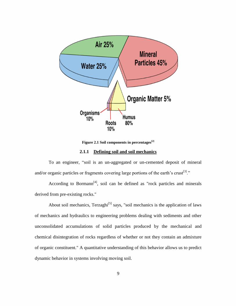
minerals, moisture, air, and organic matter as shown in Figure 2.1. Soil is classified

mainly based on its mineral components like clay, sand, and silt that define soil

composition. In addition, these minerals also define the properties like texture, porosity,

color, pH and profiles[2]

.

9

Figure 2.1 Soil components in percentages[2]

2.1.1 Defining soil and soil mechanics

To an engineer, “soil is an un-aggregated or un-cemented deposit of mineral

and/or organic particles or fragments covering large portions of the earth‟s crust[3]

.”

According to Bormann[4]

, soil can be defined as "rock particles and minerals

derived from pre-existing rocks."

About soil mechanics, Terzaghi[5]

says, "soil mechanics is the application of laws

of mechanics and hydraulics to engineering problems dealing with sediments and other

unconsolidated accumulations of solid particles produced by the mechanical and

chemical disintegration of rocks regardless of whether or not they contain an admixture

of organic constituent." A quantitative understanding of this behavior allows us to predict

dynamic behavior in systems involving moving soil.

10

Wet soil is a mixture of sand, clay, and silt suspended in fresh water. Soil is

classified based on the proportions of sand, clay, and silt. The physical properties of wet

soil depend on its composition as well as on the moisture content present in the soil. This

implies that the wet soil properties can be completely defined as a function of sand, silt,

clay and moisture content.

2.2 SOIL CLASSIFICATION

Soil seldom exists in the pure form of its minerals like sand, silt and clay.

Classification gives an idea of the properties of the soils and suitability for different

applications.

The major classification systems are

i. AASHTO (American Association of State Highway and Transportation Officials)

system

ii. USCS (Unified Soil Classification) system

iii. USDA (United States Department of Agriculture) system

All the classifications are based on grain size distribution within the soil. The

index tests such as Sieve analysis and Hydrometer analysis make use of the US standard

sieves in determining the grain size distribution. Sieve analysis and Hydrometer analysis

are standard tests adapted by Geotechnical Engineering for finding the grain size

distribution. The corresponding sizes in millimeters (mm) and the sieve numbers for the

US standard sieves are as shown in Table 2.1

11

Table 2.1 Standard sieve numbers and sizes[7]

US Standard Sieve No. Sieve Opening (mm)

4 4.750

6 3.350

8 2.360

10 2.000

20 0.850

40 0.425

60 0.250

80 0.180

100 0.150

200 0.075

Figure 2.2 represents a soil skeleton that shows the weight-volume relationships.

Soil element has three phases: air, water and solids. In a saturated soil sample, air and

water fill up the voids. It clearly explains the phase diagrams for partially saturated, fully

saturated and dry soil which helps in visualizing the soil structure. Figure 2.2 gives the

different relationships for weight - Eqn.(2.1), volume – Eqn.(2.2), moisture content –

Eqn.(2.3) and void ratio – Eqn.(2.4). Equations help us to understand the soil behavior.

Weight: t w sw w w (2.1)

Volume: t a w sv v v v (2.2)

Moisture Content: *100w

c

s

wWeightofWaterm

WeightofSolids w (2.3)

Void Ratio: v

s

vVolumeofVoidsvr

VolumeofSolids v (2.4)

12

Figure 2.2 Soil phase diagram[8]

2.2.1 AASHTO Classification System

The American Association of State Highway and Transportation Officials

developed AASHTO system. AASHTO system acts as a guide for soil classification used

by pavement engineers for highway construction and other transportation purposes.

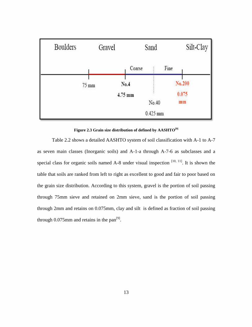
Figure 2.3 details about the grain size of the particles used in the AASHTO soil

classification system.

13

Figure 2.3 Grain size distribution of defined by AASHTO[9]

Table 2.2 shows a detailed AASHTO system of soil classification with A-1 to A-7

as seven main classes (Inorganic soils) and A-1-a through A-7-6 as subclasses and a

special class for organic soils named A-8 under visual inspection [10, 11]

. It is shown the

table that soils are ranked from left to right as excellent to good and fair to poor based on

the grain size distribution. According to this system, gravel is the portion of soil passing

through 75mm sieve and retained on 2mm sieve, sand is the portion of soil passing

through 2mm and retains on 0.075mm, clay and silt is defined as fraction of soil passing

through 0.075mm and retains in the pan[9]

.

14

Table 2.2 AASHTO soil classification system[11]

Note: LL is Liquid Limit

14

15

2.2.2 USCS Classification System

United States Army Corps of Engineers (USACE) has developed this system and

it was standardized in ASTM D 2487 as “Unified Soil Classification System (USCS)”[12]

.

Professor Casagrande‟s classification is the basis for Unified Soil Classification System

(USCS) who originally developed it for airfield construction. Later on this system was

modified and applied to foundations and dams[13]

.

This is used by geotechnical engineers, for the study of materials for construction

in geology to determine the plasticity and textural properties of soil. They use visual

observation for this classification. Figure 2.4 gives the details about the grain sizes of

different particles that are used in USCS classification.

Figure 2.4 Grain size distribution defined in USCS classification[9]

According to this system, soils are classified into coarse-grained soils (less than

50% pass through sieve No. 200) and fine-grained soils. Each group is represented with a

two lettered-symbol, one prefix and one suffix. The prefix depicts the grain size and the

suffix depicts the nature of the soil. Table 2.3 shows a detailed USCS classification of

soils.

16

Table 2.3 USCS classification[12]

Prefix: G-gravel, S- sand, M- silt, C- clay, O- ogranic

Suffix: W-Well graded, P-Poorly graded, M-Silty, L-low plasticity (LL<50%), H-High plasticity (LL>50%)

16

17

2.2.3 USDA Soil Classification System

United States Department of Agriculture has developed USDA system of soil

classification based on relative proportions of sand, silt and clay. According to this

system of classification, there are 12 varieties of soils based on soil composition. USDA

classification uses textural triangle for defining soil classes and is mainly used for the

agricultural applications. Table 2.4 gives the grain sizes for sand, silt and clay. Figure 2.5

shows the soil texture triangle with 12 major soil classes depending on the proportions of

sand, silt and clay gives a range of percentages for each soil class.

Figure 2.5 Different soil texture classes[14]

18

Table 2.4 Particle names and sizes in mm[14]

Particle Name Grain Size (mm)

Sand 0.05-2

Silt 0.002-0.05

Clay < 0.002

Table 2.5 gives us the percentages of sand, silt and clay for different soil textures.

In general, textures rich in “sand” are called sandy soils, rich in “silt” are termed as silty

soils and rich in “clay” content are identified as clay soils.

Table 2.5 Twelve differet soil textures with constituent proportions[14]

Soil texture class Sand (%) Silt (%) Clay (%)

Sand 86-100 0-14 0-10

Loamy Sand 70-86 0-30 0-15

Sandy Loam 50-70 0-50 0-20

Loam 23-52 28-50 7-27

Silty Loam 20-50 74-88 0-27

Silty 0-20 88-100 0-12

Clay Loam 20-45 15-52 27-40

Sandy Clay Loam 45-80 0-28 20-35

Silty Clay Loam 0-20 40-73 27-40

Sandy Clay 45-65 0-20 35-55

Silty Clay 0-25 40-60 40-60

Clay 0-45 0-40 40-100

19

2.2.4 Significance of USDA Classification System

USDA classification system is utilized for this research as this is a very simple

way of classifying soils and is also relevant because of its applications. In this system,

grain size distribution is studied for a given soil using the soil index tests. These index

tests are simple laboratory tests like the Hydrometer test, Sieve Analysis and Atterberg

limits that help to better understand the soils. As this research deals with off-road tires,

USDA classification of soils is best suited for analyzing the soils and soil properties.

It is easy to read the textural triangle and locate a soil sample. Figure 2.6

represents the standard texture triangle with sand, silt and clay percentages on three sides.

Percentage sand is at the bottom of the triangle which is represented by the base of the

triangle. On the sand line, sand content increases from 0 to 100% as we move from right

to left. For example, to find 50% of sand, sketch a line from the 50% mark on the sand

line (base) to the clay line (the line on the LHS of the base), such that it is parallel to the

silt line (the line on the RHS of the base). All soils with 45% sand will pass through this

line. For 20% silt, sketch a line from the 20 % mark on the silt line (the line on the RHS

of the base) to the sand line (base), such that it is parallel to the clay line (the line on the

LHS of the base). This line gives the soils that comprise of 20% silt. Similarly for 30%

clay, sketch a line from the 30% point on the clay line (the line on the LHS of the base) to

the silt line (the line on the RHS of the base), such that it is parallel to the sand line

(base). This line represents soils that have 30% clay in them. The intersection of all these

lines, which would be somewhere inside the triangle, will define the textural class for a

sample with 50% sand, 30% clay and 20% silt. The texture that was determined from this

20

composition is sandy clay and is shown in Figure 2.6. The percentages of sand, silt and

clay add up to 100 and the intersection of these three lines gives the point of reference

which is used in the research.

Figure 2.6 Soil texture triangle

2.3 SOIL PROPERTIES

Different soil properties that are important in the study of soils include physical

properties, chemical properties, static properties, and dynamic properties. This research

addresses the study of some physical properties to evaluate other properties that are not

described previously. Below are descriptions for some important soil physical properties.

21

2.3.1 Texture

Texture is defined as the size of the particles found in the soil and acts as a key

factor in defining its physical properties. It depends on the soil constituents (sand, silt and

clay) and it is mainly decided based on their percentages[17]

. Soils predominated by fine

clay particles are fine textured soils, whereas soils predominated by larger (sand and

gravel) particles are coarse textured soils; shown in Figure 2.7 which determines the

suitability of the soil for a particular application. The sand particles are large and coarse,

silt particles are small and soft while the clay particles are tiny and sticky that are

established by texture. Figure 2.8 shows the texture triangle with various fineness.

Figure 2.7 Soil texture [15]

Figure 2.8 Soil texture triangle depicting fineness of soils[15]

22

Soil texture influences many other physical properties like porosity, permeability,

moisture retention capacity and the surface of soil particles. Table 2.6 gives the

comparison of different properties for soil constituents; sand, silt and clay based on the

property of soil texture. In the upper part of the texture triangle shown in Figure 2.8, the

fineness of soils decreases from top to bottom, while in the lower part the fineness

decreases from right to left. The properties compared in Table 2.6 are described as below:

i. Porosity is the ratio of volume of voids to volume of soil[18]

.

ii. Permeability is the ability of a particle to allow the flow of water under excess

pressure[19]

.

iii. Moisture retention capacity is the ability of a particle to hold water[20]

.

iv. Soil particle surface is the surface that gets in contact with other particles[9]

.

Table 2.6 Comparison of different soil properties for sand, silt and clay[21]

Property Sand Silt Clay

Porosity Large pores Small pores Small pores

Permeability Quick Slow to Moderate Slow

Moisture retention

capacity Very little Moderate Very high

Soil particle surface Large Medium Very large

All the above mentioned properties help to understand the soil stickiness and also

to find the standard composition for a sticky soil. As clays have high moisture retention

capacity, sticky soils can have high clay content. Further, sticky soil cannot have more

sand particles, as all the moisture gets drained through the large pores and gets settled at

bottom.

23

2.3.2 Stickiness

Stickiness is defined as the property of a wet soil to adhere to another object[20].

We measure stickiness at whatever point the thumb and forefinger stick to each other,

when wet soil is squeezed between them. Testing the soil with hand, between fingers is a

standard test called “feel test” for soils[22]

. There are three major stickiness classes: Non-

sticky, Moderately sticky and very sticky. Feel test does not give any quantitative

measure of stickiness, though it is considered to be a standard test in geotechnical

department. The results from feel test cannot be consistent as different persons might

carry out the tests and the force applied on the sample depends on the person and it

cannot be the same always.

Below is the description for each of them along with a picture of wet soil samples.

Non-Sticky – little or no soil sticks and remains between thumb and forefinger[23,

24]. Figure 2.9 shows a sample of non-sticky soil between two fingers and this shows no

soil is stuck to the upper finger when two fingers squeeze the wet soil between them.

Figure 2.9 Non-sticky soil sample[25]

24

Moderately Sticky – wet soil sticks to both fingers and fingers separate with

some stretch. Figure 2.10 shows a sample of moderately sticky soil between two fingers

and this shows some soil is stuck to the fingers when two fingers are pressed towards

each other.

Figure 2.10 Moderately sticky soil sample[25]

Very Sticky - wet soil sticks firmly to both fingers i.e. thumb and forefinger[23, 24]

.

Figure 2.11 shows a sample of sticky soil between two fingers and this shows more soil is

stuck to the fingers when two fingers squeeze the wet soil.

Figure 2.11Very sticky soil sample[25]

25

2.3.3 Cohesion and Adhesion

Cohesion is the attraction between similar molecules i.e. between water

molecules[5]

. It is mainly due to the electrostatic force between the particles.

Mathematically, it is inversely proportional to the square of the distance between two

particles. Hence, cohesion and particle size are inversely proportional i.e. the greater the

distance, the smaller the cohesion value. Wet sand exhibits noticeable cohesion and sand

in its dry condition do not exhibit any cohesion. Tensile failure of a soil gives us a

measure of cohesion. When soil fails under tension, the normal stress becomes zero and

only component that causes resistance is cohesion.

Adhesion is the attraction of a water molecule to a non-water molecule[5]

.

Adhesion is mainly due to a moisture film at the contact surface which is found out from

soil properties, roughness of the surface and moisture content[26]

. Use of more water

content increases soil adhesion to the lug surface. Hence, in our research effort has been

made not to have more moisture content when finding a sticky mixture. Performance, in

terms of distance travelled by a vehicle, and efficiency of the equipment used in the field,

reduces with soil adhesion[27]

. The problem of adhesion with off-road tires is that been

predicted recently.

2.3.4 Plasticity

Plasticity is the degree to which soil is deformed and reworked permanently

without rupture[6]

. It is the ability of soil materials to change their shape continuously

under the influence of a constant pressure and retain its impressed shape even after

removing the applied pressure. This is measured by an index soil test used for defining

26

the liquid limit. Plasticity is determined by rolling a wet soil sample between the hands to

make a 3-mm (1/8 –in) cylinder. The point during rolling on the glass plate, at which the

rolled wet soil breaks (because the soil dries) is known as the plastic limit[28]

.

2.3.5 Atterberg Limits

Wet soil has rheological properties, which cannot be referred to either as solid

property or as fluid property. This implies that wet soil functions more towards the plastic

behavior of a material when put in a continuum between fluid and solid. In general, the

plastic limit is a lower bound and the liquid limit is an upper bound of wet soil. These

bounds are together called Atterberg limits. The Atterberg limits test is used to calculate

the bounds for plasticity index(PI)[29]

. PI of a soil is a range of water content where a

given soil behaves as a plastic material. Soil also behaves as a Non-Newtonian fluid in PI

range.

Liquid Limit (LL)

Liquid limit is defined, as “the water content required for rendering the soil just

fluid as distinct from plastic”[6]

. It is the amount of water present in the soil when the soil

moves under the influence of continuous forces.

Liquid limit is measured by applying, the paste made of the soil residue from the

fourth sieve (sieve opening of 0.425mm) to a round-bottomed brass cup. The extra soil in

this cup is removed by leaving the paste thickness to a maximum of 10mm. The soil that

is spread in the cup is divided into two halves with a small grooving tool. The whole

arrangement has a crank and it helps in hitting the cup to the base. After 25 blows, if we

27

observe that groove closes, the water content present in that soil gives the liquid limit for

that soil sample.

Plastic Limit (PL)

Plastic limit is defined as “the water content in percent at which the soil crumbles,

when rolled into threads of 3.2 mm (1/8 in) in diameter”[6]

. It is the minimum water

content at which the mixture acts as a plastic solid.

Plastic limit is measured by rolling the wetted soil with the palm of the hand on a

frosted glass (mildly absorbent surface) into a thread or worm of soil 3 mm (1/8 in)

diameter. This is repeated (soil gradually dries while being reworked several times) until

the thread breaks up into short pieces as the rolling soil thread approaches the 3 mm

diameter. This water content where the thread breaks is the plastic limit.

Plasticity Index (PI)

Plasticity index (PI) is the difference between the liquid limit and the plastic limit

of a soil[9]

. It is the range of water content within which the soil exhibits the properties of

a plastic solid; it is a measure of the cohesive properties of the soil. Soil becomes more

sensitive to plastic deformation with increase in the plastic index[30]

. A material is termed

as “silty” if it has a PI of 10 or less and as “clayey” if it has a PI of 11 or greater, after

rounding off to the closest whole number. Plastic nature of a soil depends on the PI and

the soil deformation increases with the PI.

PI LL PL (2.5)

where,

LL is liquid limit of the given soil and

28

PL is plastic limit of the given soil

Eqn.(2.5) gives a mathematical equation for plasticity index.

2.4 SOIL WATER CONTENT

Soil water content is the amount of water vapor that is lost from a soil sample

when heated to 1050C, until the weight loss becomes almost zero

[31, 32] i.e. it indicates

how much water is present in a soil sample.

A simple test is conducted in the laboratory to study the moisture loss in potting

soil. In terms of mass ratio, the unit of soil water content is kg kg-1

(kg water per kg dry

soil) and in terms of volumetric ratio, the unit is m3m

-3 (m

3 water per m

3 of bulk soil

volume).

2.4.1 Thermo Gravimetric Method

A direct method of measuring the moisture loss to measure the soil water content

is the thermo gravimetric method. A measured quantity of soil sample is heated for 24hrs

in a microwave oven at 1050C using an insulated container. This method of drying soil is

called microwave drying. Remove the soil sample after 24hours and weigh it to measure

the weight loss. This process is repeated till the mass difference between two consecutive

readings become equal. The moisture loss for the sample „w‟ is the ratio of mass of water

per unit mass of dry soil. Eqn.(2.6) gives the mathematical expression for finding the soil

moisture content in terms of weight percentage[32]

.

* 100massofwetsoil massofdrysoil

massofdrysoilw

-= (2.6)

29

It is necessary to ensure zero percent moisture content in sand, silt and clay before

making the soil samples in the laboratory. Slight change in water content might change

the soil properties. Soil water accounts for cohesive and adhesive forces and hence soil

water plays an important role in this research.

2.5 SOIL DYNAMICS

Soil dynamics deals with soils under motion and is defined as a relation between

applied forces to a soil and its reactions. Mechanical forces applied on the soil, cause

these reactions. Soil dynamics has been used in tillage and traction since 1920 but the

research in this area has increased from 1950[26]

.

2.5.1 Dynamic Properties of Soil

The properties of a soil observable and established by soil movement are termed

dynamic properties of soil. Some of the dynamic properties of soil are friction, stress,

strain and strength. We observe friction between a surface and a block of soil, when

block of soil is moved from stationary to mobile state, motion is necessary to determine

such a property. The strength of the soil increases as the loose soil is compressed and

hence strength is a dynamic property of soil. Forces acting on a block of soil that moves

cause deformation in terms of physical displacement. It is difficult to measure these

properties, as one has to measure them under action and high deformation.

2.5.2 Soil Stress

The study of forces acting on a small finite block of soil is easy as it requires a

vector representation of different forces like friction, gravity and mechanically applied

forces. But it is difficult to study the forces that act on soil in a semi-infinite channel as

30

the forces are distributed over a channel. The mathematical formulation of stress as force

per unit area cannot be applied in such circumstances.

The semi-infinite channel is a 3-D medium where both the direction and area are

unknown. Study of forces is carried out by applying the state of a stress concept and is

applicable for continuous materials. Even though, soil is porous, to calculate the stress in

the soil that is packed in a semi-infinite channel, it is assumed to be in continuum.

Neglecting the pores is justified only when the area of soil is much larger than the pores.

Since a finite area is required when dealing with a soil mass, either for measurements or

for physical manipulation, the assumption of the continuum appears to be justified as

long as the smallest area considered is physically much larger than the pores or individual

aggregates of the soil [33, 34]

.

Figure 2.12 describes nine different forces that act on a soil element. Assuming

symmetry for the soil block, shear strengths, τxy= τyx, τxz = τyx, τzx, and τyz= τzy. This

symmetry eliminates three of the unknown quantities.

Figure 2.12 Normal and shear stresses on and within a soil element[26]

31

2.5.3 Soil Strain

The force applied to soil is usually described both within and on the soil mass.

Hence, the deformation must be appropriately described. Strain at a particular point has

to be determined in detail and strain at other points is calculated relative to this point[26]

.

For longitudinal elements, the basic equation for calculating engineering strain is shown

in Eqn.(2.7).

0

0

l l

l

(2.7)

where,

ε is the longitudinal strain

l is the initial length

l0 is the final length of the element

Assuming the soil to be in continuum, the longitudinal strain is expressed with the

help of differential calculus using Eqn.(2.8).

0

dld

l (2.8)

Where,

dε is the differential value of ε

dl0 is the differential value of l

2.5.4 Soil Strength

Soil strength generally refers to shear strength and is defined as the resistance per

unit area to deformation by continuous soil displacement. It is the maximum strength of

the soil where a considerable plastic deformation takes place in a soil due to applied shear

32

stress[35]

. Shear strength is mainly due to three factors; cohesion and adhesion,

interlocking between particles and frictional resistance between particles[36]

. There is no

fixed soil shear strength as depends on various factors. According to Poulos[37]

, shear

strength depends on soil composition, soil state, soil structure and type of loading. With

wetting, strength of the soils decrease[38]

. Soils exhibit wide range of strength values due

to soil motion when the force is applied. Hence, it is described as a dynamic property of

soil. Use of artificial soils or manmade soils facilitates the study of soil strength, as it is

consistent in such cases. Strength of the soil increases when it is compacted. Strength

change becomes obvious when large volume of soil is in compaction. Table 2.7 shows

large variation in strengths of samples taken from different geographic regions. This

illustrates the high variability of soil strength based on composition.

Table 2.7 Variation in strength[26]

Type of soil Tensile Strength Compressive Strength

Sample 1 52 86

Sample 2 51 125

Sample 3 135 342

Sample 4 182 357

2.5.5 Stress-Strain Relationship

The dynamic properties of soil have not been clearly defined and more research is

going on in soil dynamics. At present, many stress-strain relationships have been

developed which do not give the actual plastic behavior of soils. Assuming soil as a strain

hardening material, a model is developed. This developed model is validated using the

model derived from the compaction test. If the stress is small, the soil may deform

33

slightly and reach an equilibrium condition through the storage of energy within the

mass. Release of the stress will allow the soil to return to its original position. Yielding of

soil may result in a redistribution of the load, a new and different state of equilibrium, or

movement of the soil so that the load decreases or is no longer in contact with the soil[39]

.

Soil deformation has a time dependent property that is not reconciled by plastic and

elastic theories. The relationship between true stress and true strain is acquired by a

compaction test using a tensile testing machine, and is described in Chapter 4.

2.6 CHAPTER SUMMARY

This chapter dealt with the classification of soils and significance of USDA

system to the research, description and importance of various physical soil properties,

dynamic properties, relation between soil composition and its properties. The importance

of these properties in improving the self cleaning capability of a rubber channel is

discussed. The next chapter deals mainly with testing soils using various Index tests to

find out the grain size distribution of a specific soil sample (potting soil), its composition

texture, and plasticity index. Based on potting soil composition as a baseline, some sticky

soil compositions are recognized. The next chapter will also deal with the description of

moisture content, and its effect on the nature of a soil. Experimental results for each test

are mentioned in detail.

34

CHAPTER 3

3 SOIL PROPERTY TEST METHODOLOGY

The main objective of this chapter is to establish a testing methodology to

determine composition, soil plasticity and adhesiveness. Standard soil testing

methodology used in Geotechnical Engineering has been applied to the soil samples to

determine the composition and plasticity. The tests that evaluate the composition of a soil

and also define the properties are called as soil index tests. These tests are comprised of

Sieve Analysis, Hydrometer Analysis and Atterberg limits test. Sieve analysis and

Hydrometer analysis collectively give the grain size distribution. With the help of grain

size distribution, we can obtain the soil composition. When this composition is located

on the texture triangle, it gives the texture class of the given soil. The texture triangle has

twelve textural classes and each of them behaves differently in terms of porosity,

permeability, and moisture retention capacity, which fall in to the category of soil

physical properties. Hence, the composition also determines the soil properties.

Atterberg limits test is used to compute the plastic limit, liquid limit and plasticity index.

Addition of water content to dry soils, change the nature of soil from solid-semisolid-

plastic-liquid. Atterberg limits test gives a dividing line between these phases and also a

range, for the plastic behavior of soils. Plasticity index also helps in finding the soil

composition. There are other physical properties which cannot be determined using these

index tests.

A new methodology is developed to study the soil properties that are not

illustrated by the index tests. This resulted in two new laboratory tests, namely Drop test

35

and Rotating Arm test. These tests determine the wet soil fly off speed and adhesiveness

of various soil samples. This new methodology helps in testing tire treads in combination

with various soil samples and also recognizes a relatively adhesive soil composition.

Drop test is packing a tire tread (or any rubber sample with channels) with wet

soil and dropping it from different heights. As a result of this, wet soil flies off the

grooves or channels. When different soil samples are tested in this manner, the relative

amount of mass loss during the test, in the form of fly off soil, helps us in finding a

relatively sticky soil. These tests are also helpful in studying the effect of water content

on the adhesiveness. Consequently, the results obtained from these tests acts as the

starting values for finding a relatively sticky soil composition. The linear drop apparatus

is simple and manually controlled.

The Rotating arm test is used to simulate the tire tread sample as tire under

rotation. In drop test, wet soil fly off is linear while in rotating arm test, it follows a

circular path. The rotating arm is fixed to a wheel balancer which operates with the help

of a motor. This rotational movement is similar to a tire rotation of a vehicle. The rotating

arm is accelerated with the help of the motor to simulate the tire behavior. Soil that is less

sticky flies off very quickly when compared to sticky soil. Rotating arm apparatus is

motor controlled and is more complex as compared to the drop apparatus. It is important

to keep the tire sample under rotation in rotating arm for clear understanding of tire

behavior.

The first section in this chapter deals with index tests on the initial potting soil

sample to find its grain size distribution and composition. Second section deals with the

36

experiments carried out on drop test apparatus to identify the adhesive soil sample among

the samples considered.

3.1 INDEX TESTS

Index tests are standard tests used for soil classification based on particle size

distribution. The distribution of soil particles which are termed as grains is determined

based on Sieve Analysis and Hydrometer Analysis. Atterberg limits analyses will predict

the plastic limit, liquid limit and plasticity index that help in the determination of water

content required, changing a soil from semi-solid to plastic, and if more moisture is

added, soil will enter into the liquid phase thereby losing its plastic nature. Plasticity

index gives the range in which a soil can be plastic. A plastic mixture can be sticky.

Figure 3.1 is a pictorial representation of index tests and are explained in the next

sections of this chapter.

Figure 3.1 Pictorial representation of the index tests

37

3.1.1 Sieve Analysis

Sieve analysis determines the particle sizes of soil constituents and quantitative

distribution of dry soils. This test shows the particle size distribution for particle sizes

bigger than 0.075mm. The method used for evaluation of particle size distribution

depends on the particle sizes that have to be tested i.e. if the particle is bigger than

0.075mm, Sieve analysis is used and if the particle size is smaller than 0.075mm,

Hydrometer analysis is used. Soil samples with zero moisture content are used for testing.

Any kind of mass loss either moisture loss or mass loss to surroundings, is neglected if it

is less than 2%. The aim of this test is to find the grain size distribution of any soil, but

potting soil sample is considered in this section.

For soils that have a maximum particle size of 4.75mm, 500gms of dry soil is

used and particles greater than 4.75mm require more dry soil. It is advisable to pulverize

the soil sample using a mechanical crusher, if it has large lumps. When 500gm of soil is

dried in an oven to remove the moisture , its mass came down to 480gm and this 480gm

is used for the sieve analysis. Mass loss here is 20gm which is 0.05 % < 2% and hence, it

is neglected.

Apparatus

The apparatus required for carrying out Sieve analysis is set of sieves (Figure

3.2), mechanical shaker (Figure 3.3), drying oven (Figure 3.4), weighing balance

calibrated to 0.1gm (Figure 3.4), rubber pestle and mortar to break large soil lumps

(Figure 3.4).

38

Figure 3.2 Sieve arrangement based on opening size [7]

Figure 3.3 Mechanical shaker[7]

39

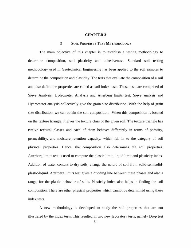
Figure 3.4 Drying oven, weighing scale and rubber pestle and mortar

Procedure

The steps involved in the Sieve analysis test are as follows:

i. Initially 480gm of oven dried soil sample is taken and is broken down into smaller

particles with a rubber pestle and mortar

ii. Mass of the sample (Mi) is measured using the weighing scale

iii. Stack of sieves are arranged from larger to smaller according to the opening size

iv. The topmost sieve is covered with a lid to fix it to the shaker and it also avoids

soil fly-off; remaining sieves rest on a pan that collects the finer particles

v. Soil sample prepared earlier are taken into the first sieve and is covered with the

lid on top

vi. With the help of mechanical shaker, sieve stack is shaken for 15mins and it causes

the soil particles to pass through the sieves and retain on a particular sieve based

on their grain size

40

vii. After the test, the set of sieves are removed and the soil that is retained on each

sieve as well as in the pan is weighed

viii. The mass of soil retained on each sieve is added which gives the cumulative mass

(Mf)

ix. From this, percent mass retained on each sieve, cumulative percent of mass

retained(CR) and percent finer are calculated

x. Percent finer is calculated using Eqn. (3.9)

100Percentfiner CR= - (3.9)

xi. Mass loss (m) during this analysis is calculated using Eqn. (3.10).

*100i f

i

M Mm

M

-= (3.10)

where,

m - Mass loss in percentage

Mi - Initial mass of the sample

Mf- Final mass of the sample

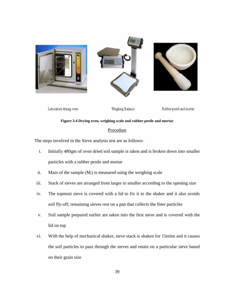
Results

The grain size distribution is analyzed with the results from sieve analysis test.

Calculations are made to find out percent finer and a graph is plotted with sieve opening

on x-axis and percent finer on y-axis (shown Figure 3.5). This is called the grain size

distribution graph. The grain size distribution for potting soil is as shown in Figure 3.5.

41

Table 3.1 Results obtained from Sieve analysis

Figure 3.5 Grain size distribution obtained from Sieve Analysis

Sieve No. Sieve

opening (mm)

Soil retained

(gm)

Mass

retained in %

Cumulative

Mass in %

Percent

finer

4 4.75 41.00 8.56 8.56 91.44

10 2.00 102.00 21.30 29.87 70.13

20 0.85 106.00 22.14 52.01 47.99

40 0.43 84.00 17.54 69.55 30.45

60 0.25 49.00 10.23 79.78 20.22

100 0.15 37.00 7.73 87.51 12.49

200 0.08 28.00 5.85 93.36 6.64

Pan

31.00

42

Discussion

The sample that is used for this test is standard potting soil. The sample mass

taken is 480gm and cumulative mass that retains on all the sieves and pan is 478.8gm.

This shows, there is a mass loss of 1.2gm to the surroundings which is 0.25%

(negligible). Figure 3.5 shows a graph plotted for percent finer (%) and sieve opening

(mm) to explain the grain size distribution which shows the distribution of particles in

each sieve and it gives the amount of sand particles. The amount of soil that is retained on

each sieve is weighed, and with the help of the sieve opening size, the particles are

classified into coarse grains and finer grains. This leads to Hydrometer analysis which

runs with the amount of soil that is retained on Sieve No. 200 of the stack of sieves.

3.1.2 Hydrometer Analysis

Hydrometer test is carried out to determine the particle size distribution for

particles smaller than 0.075mm (particles that are collected from sieve analysis after

passing through sieve No. 200) i.e. to find the grain size distribution in a soil from the

coarse sand to the clay size. Figure 3.6 shows the soil hydrometer used for hydrometer

analysis[40, 41]

.

Apparatus

The apparatus used for Hydrometer analysis are soil hydrometer (Figure 3.6), two

1000ml glass cylinders (marked in ml), deflocculating agent (Calgon), stop clock, glass

rod, constant temperature bath, mixer, distilled water, beaker, spatula, weighing balance,

plastic squeeze bottles and rubber stopper for the cylinder.

43

Figure 3.6 Soil hydrometer[42]

Procedure

The procedure for Hydrometer analysis consists of the following steps:

i. 50gm of oven-dried soil sample is taken in a beaker by using a weighing balance

which has 0.01gm accuracy

ii. A deflocculating agent is made by adding 40gm of Calgon (chemical name of

calgon is sodium hexametaphosphate) to 1000ml of distilled water in a cylinder

and mixed thoroughly

iii. 125ml of deflocculating agent prepared in step (ii) is now added to 875ml of

distilled water in a 1000ml cylinder

iv. Soil sample is added to this mixture and stirred well while the cylinder is kept in a

constant temperature bath

44

v. The hydrometer is immersed in the cylinder and the readings are taken at the

upper meniscus of hydrometer at different time periods

vi. Readings are taken at the intervals of 0.25min, 0.5min, 1min, 2min, 4min, 8min,

20min, 32min, 65min, 123min, 240min, 480min, 660min and 24hr

vii. The hydrometer is removed and inserted after each reading to avoid errors

viii. The initial and final temperatures of the bath are also recorded

ix. Percent finer is calculated using the Eqn.(3.11)

*a HR

Percentfinerw

= (3.11)

where,

a is the correction factor calculated using the Eqn.(3.12)

(1.65)

( 1)2.65

s

s

Ga

G=

- (3.12)

Here, Gs = 2.65 (specific gravity of the used hydrometer) hence a = 1.00 (using

Eqn.(3.12))

HR is hydrometer reading

w is initial weight of the sample

Diameter is calculated using Eqn.(3.13)

( )

( )(min)

L cmD mm A

t= (3.13)

where,

A is 0.0135 (for Gs = 2.65, from standard table)

L is effective length for corresponding CHR

45

Results

The results for hydrometer analysis with potting soil are as shown in Table 3.2.

Column 3 gives the percent finer values which are plotted on a graph shown in Figure

3.7. This also gives the diameter of the particle. Mass loss in hydrometer analysis is

neglected. Errors during the experiment i.e. parallax error in taking hydrometer readings

is neglected in this test. With the results obtained from Sieve analysis and Hydrometer

analysis, a combined graph with grain size (mm) on x-axis and percent finer (%) on y-

axis is plotted and is shown in Figure 3.7.

Table 3.2 Hydrometer test results for potting soil

Time, t

(min)

Hydrometer

Reading, HR

Percentage

Finer (%)

Corrected

Hydrometer

Reading, CHR

Effective

length, L

(cm)

Diameter, D

(mm)

0.25 29 54.44 30 11.4 0.085

0.5 27 50.52 28 11.7 0.0612

1 25 46.6 26 12.0 0.0438

2 24 44.64 25 12.2 0.0312

4 22 40.72 23 12.5 0.022

8 21 38.76 22 12.7 0.016

20 19 34.84 20 13.0 0.01

32 18 32.88 19 13.2 0.008

65 13 23.08 14 14.0 0.005

123 12 21.12 13 14.2 0.004

240 11 21 12 14.3 0.003

480 11 20.5 12 14.3 0.002

660 11 19.9 12 14.3 0.0018

46

Figure 3.7 Grain size distribution obtained from Hydrometer analysis

Discussion

Figure 3.7 gives the grain size distribution for particles greater and smaller than

0.075mm. The results are as expected i.e. Sieve analysis depicts the particle size

distribution for particles greater than 0.075mm and Hydrometer analysis expresses the

particle size distribution for particles smaller than 0.075m.

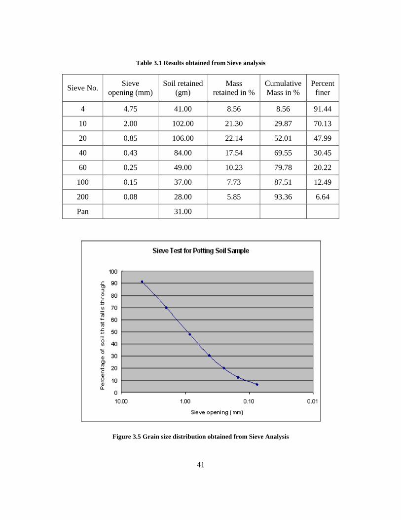
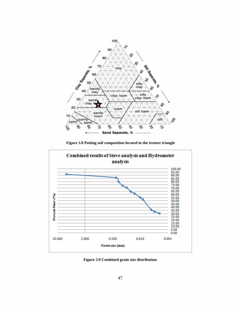
Figure 3.9 gives the combined grain size distribution for Sieve analysis and

Hydrometer analysis. From these results, the composition of the potting soil is estimated

to have 57% sand, 19% silt and 24% clay. This is identified as the sandy clay loam

category of soils (Figure 3.8) which are not sticky and feels rough and gritty. Following

the existed literature, this soil was judged as non-sticky soil[43]

. Hence, these results

concluded that potting soil is not sticky.

47

Figure 3.8 Potting soil composition located in the texture triangle

Figure 3.9 Combined grain size distribution

48

3.1.3 Atterberg Limits Test

The aim of running the Atterberg limit tests is to confirm the particle size

distribution and to determine the liquid limit, plastic limit and plasticity index for potting

soil sample. This gives us the amount of water that can be added to a make a fairly sticky

soil sample.

Description

The effect of moisture can be explained by the consistency limits. Figure 3.10

shows soil consistency based on plastic limit and liquid limit. Liquid limit test gives the

liquid limit, plastic limit test gives the plastic limit, and their difference gives us the

plasticity index for the given sample. When excess water is added to a cohesive soil, it

flows like a viscous liquid. When this resultant is gradually dried using an oven, it enters

into a plastic zone[10, 41, 44]

. When the soil is still dried it enters the semi-solid zone and

then finally into the solid zone. This criterion is explained clearly using Figure 3.10.

Figure 3.10 Soil consistency based on Atterberg limits[45]

49

Figure 3.11 shows the equipment required for the Atterberg limits test(liquid limit

test and plastic limit test). They include Casagrande device (device with brass cup in

Figure 3.12 invented by Dr. Casagrande to calculate the plastic limit), grooving tool,

drying oven, moisture drying cans, spatula, evaporating dish, weighing balance calibrated

to 0.01gm, distilled water, squeeze bottles, and glass plate.

Figure 3.11 Equipment for Atterberg limits tests[46]

Liquid Limit Procedure[28]

i. 250gm of the air-dry potting soil that passes through sieve no. 40 is taken in an

evaporating dish and water is added to it with the help of squeeze bottles

ii. It is mixed till it becomes a uniform paste

iii. A part of this paste is applied evenly to the brass cup or casagrande cup

iv. With the help of spatula, it is smoothly distributed keeping the maximum depth of

the paste to 8mm

v. Weight of the moisture cans are measured as m1

50

vi. A groove is made at the center of the cup using the grooving tool as shown in

Figure 3.15

vii. Now with the help of the crank rotation, the cup is made to hit the device

viii. The blows go on till soil from both the sides of the groove move towards the

center and close the groove

ix. The number of blows are counted as n and in the first trial n value lies between 25

and 35

x. Soil paste is removed and put in one of the moisture cans and weighed as m2

xi. The cup is cleaned with the help of paper towels and this test fails if the number

of blows go more than 35 which can be concluded as a dry soil

xii. More water is added to the soil and same procedure is continued taking n value

between 20 and 25, corresponding moisture can with moist soil is weighed

xiii. Finally, n is kept between 15 and 20 and moist soil with the can is weighed

xiv. All the three moisture cans are put in the drying oven till constant mass is

achieved and are weighed as m3

xv. All the values are entered into a table

xvi. Moisture content for each trial is determined using the Eqn.(3.14)

2 3

3 1

(%) *100m m

wm m

-=

- (3.14)

xvii. A semi-log graph is plotted between moisture content, w and number of blows, n

xviii. This gives a straight line and a dotted line parallel to y-axis is drawn at n = 25

51

xix. From this intersection point, another dotted line parallel to x-axis is projected onto

the y-axis

xx. This gives the liquid limit for the given potting soil sample

Figure 3.12 Casagrande apparatus[47]

Results

Table 3.3 gives us the readings taken from liquid limit test. The moisture content

for each trial is calculated and included in the results table. Figure 3.13 is the plot

between moisture content (%) and number of blows and it is determined as 37%.

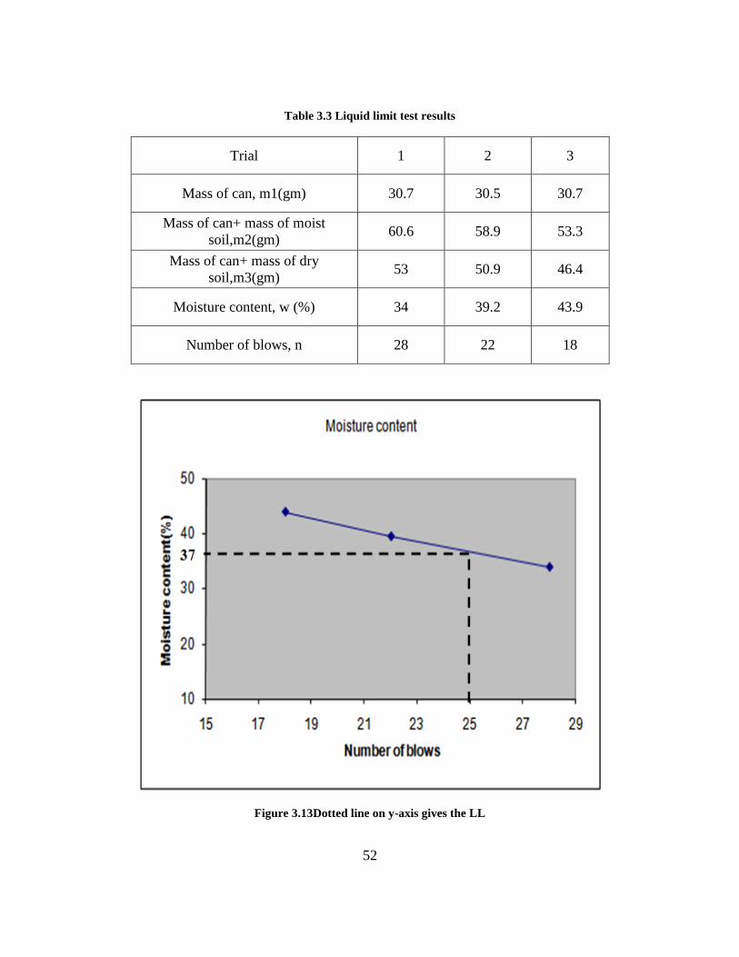
52

Table 3.3 Liquid limit test results

Trial 1 2 3

Mass of can, m1(gm) 30.7 30.5 30.7

Mass of can+ mass of moist

soil,m2(gm) 60.6 58.9 53.3

Mass of can+ mass of dry

soil,m3(gm) 53 50.9 46.4

Moisture content, w (%) 34 39.2 43.9

Number of blows, n 28 22 18

Figure 3.13Dotted line on y-axis gives the LL

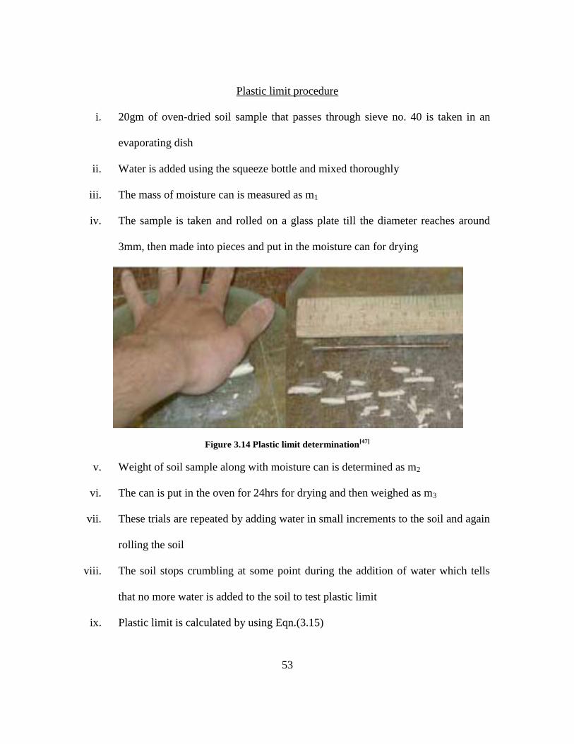
53

Plastic limit procedure

i. 20gm of oven-dried soil sample that passes through sieve no. 40 is taken in an

evaporating dish

ii. Water is added using the squeeze bottle and mixed thoroughly

iii. The mass of moisture can is measured as m1

iv. The sample is taken and rolled on a glass plate till the diameter reaches around

3mm, then made into pieces and put in the moisture can for drying

Figure 3.14 Plastic limit determination[47]

v. Weight of soil sample along with moisture can is determined as m2

vi. The can is put in the oven for 24hrs for drying and then weighed as m3

vii. These trials are repeated by adding water in small increments to the soil and again

rolling the soil

viii. The soil stops crumbling at some point during the addition of water which tells

that no more water is added to the soil to test plastic limit

ix. Plastic limit is calculated by using Eqn.(3.15)

54

2 3

3 1

*100m m

PLm m

-=

- (3.15)

Results

Table 3.4 gives the readings from plastic limit test for all the three trials. The last

row in the table gives us the plastic limit values computed using Eqn.(3.15).

Table 3.4 Readings and calculations for plastic limit test

Trial 1 2 3

Mass of can, m1 30.7 30.5 30.7

Mass of can+ Mass of moist soil,

m2 (gm)

56.2 55 56.7

Mass of can+ Mass of dried soil,

m3(gm)

52.6 51.5 53.3

PL (%) 16.4 16.6 15

3.1.4 Discussion

The plastic limit is determined as 16 from the above results. Since, the liquid limit

estimated for the sample is 37, the plasticity index is found to be 21 (calculated using

Eqn.(2.5)). These results reveal that the plastic nature of soil is exhibited when the

moisture content is between 16% and 37%. By varying water content within this range,

samples are tested for stickiness. As earlier, there was no bound for adding moisture

content and the Atterberg limits defined the upper and lower limits for moisture content

in a soil.

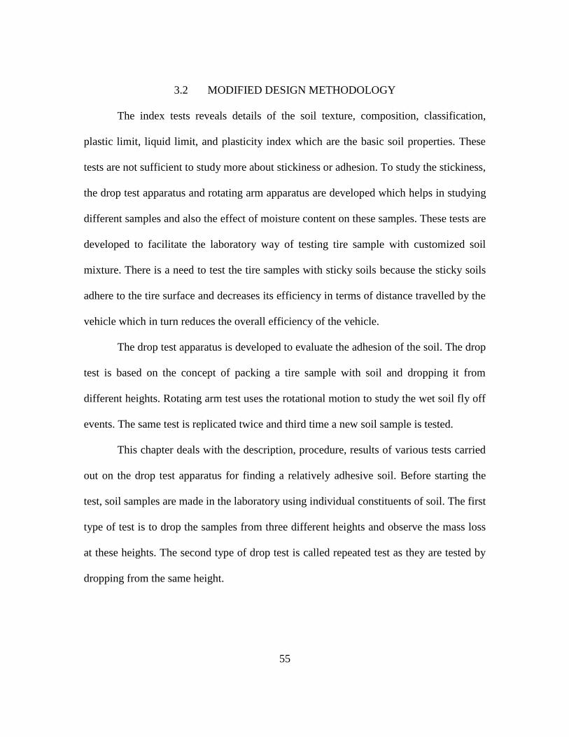
55

3.2 MODIFIED DESIGN METHODOLOGY

The index tests reveals details of the soil texture, composition, classification,

plastic limit, liquid limit, and plasticity index which are the basic soil properties. These

tests are not sufficient to study more about stickiness or adhesion. To study the stickiness,

the drop test apparatus and rotating arm apparatus are developed which helps in studying

different samples and also the effect of moisture content on these samples. These tests are

developed to facilitate the laboratory way of testing tire sample with customized soil

mixture. There is a need to test the tire samples with sticky soils because the sticky soils

adhere to the tire surface and decreases its efficiency in terms of distance travelled by the

vehicle which in turn reduces the overall efficiency of the vehicle.

The drop test apparatus is developed to evaluate the adhesion of the soil. The drop

test is based on the concept of packing a tire sample with soil and dropping it from

different heights. Rotating arm test uses the rotational motion to study the wet soil fly off

events. The same test is replicated twice and third time a new soil sample is tested.

This chapter deals with the description, procedure, results of various tests carried

out on the drop test apparatus for finding a relatively adhesive soil. Before starting the

test, soil samples are made in the laboratory using individual constituents of soil. The first

type of test is to drop the samples from three different heights and observe the mass loss

at these heights. The second type of drop test is called repeated test as they are tested by

dropping from the same height.

56

3.2.1 Drop Test

Figure 3.15 shows the drop apparatus that is developed with the idea of studying

the adhesiveness of a soil. The drop apparatus is compact and easy to use as it is

manually controlled. It is based on the concept that when an assembly comes to a sudden

stop, force is exerted on the assembly components. The drop apparatus has an

arrangement for free fall motion of an assembly to hold the tire tread sample. Large

screws called stops are arranged at 0.25m above the ground level such that the assembly

comes to a rest when it hits these screws. As a result of this, force is exerted on the wet

soil in the grooves and expels it out. This expelled mass is considered as the mass loss

during the experiments.

Figure 3.15 Linear drop apparatus

57

Experiments carried out on the drop apparatus examine the behavior of different

customized wet soil mixtures to find relatively sticky composition and also to compare

the stickiness or adhesiveness between the different manmade soil compositions to the

potting soil. Stickiness is assessed by the wet soil loss during the drop test events. Using

these tests, the effect of water content on the stickiness is also studied. Three replications

for each sample (different composition mixtures) are run for achieving consistent results.

In the first two replications, the water content is constant and in the third replication, it is

changed because a fresh batch of wet soil had to be made. A wet soil with this

composition can be used in future experiments on the drop apparatus and rotating arm to

study the fly off events of wet soil from an off-road tread sample.

Description

The interest in finding a wet soil mixture which is significantly stickier than the

previously used wet potting soil is to provide a soil sticky enough to provide good test

discrimination for release from an off-road tire tread. The soil sample that is used on the

drop test has 45% sand, 20% silt, 35% clay and 25% water content.

For the first set of tests, the tire sample is dropped from 0.75m, 0.5m and 0.32m.

Three different customized samples of wet soil are made using different proportions of

sand, silt, clay and water. Two replications are carried with these samples to study the

repeatability of results. The third set of tests is run with samples that have similar dry soil

composition, but with change in the moisture content. According to the soil texture

triangle, these three samples fit into the sandy clay soils class. It is a norm in the literature

to consider sandy clay, silty clay and clay soil as sticky soils. Generally sandy clay, silty

58

clay and clay soils are considered to be the sticky soils with the available literature on wet

soil[23]

. Figure 3.16 shows the wet soil samples that are used for replication tests. Sample

1 looks brighter because it has more clay content in it.

An important variable is the amount of water content added to each mixture.

There is no standard method for determining the amount of water to be added to the dry

constituents in order to achieve a standard elasticity or “stickiness”. Accordingly, water is

added in small increments to change the soil from a dry crumbly state to a state with

maximum stickiness by touch. Too much water makes the mixture too runny and soupy.

The water content is measured; however the overall method remains very subjective.

Table 3.5 shows a list of soil compositions which are initially tested using the “feel test”

to find the sticky samples among the considered samples. The first three compositions in

the table are found to be stickier among all the samples and are used for the drop tests. In

the table, the composition i.e. sand, silt, and clay percentages, for each sample is

mentioned along with the water content. Sample 1 has the highest clay content. The water

content varies from 20 to 26% for these customized mixtures. The water content is very

high in potting soil i.e., 32.5%. Potting soil has some extent of organic matter and that is

the reason for adding more moisture content to potting soil. Generally, the presence of

organic matter contributes to the stickiness of a sample and also holds more water

content. Sample 2 and 3 have same clay content but we can observe the significant

change in water content added.

59

Table 3.5 Comparison between three soil samples and potting soil

Sample Sand (%) Silt (%) Clay (%) Water content (%)

1 45 20 35 25

2 65 15 20 20.5

3 60 20 20 23.4

4 40 15 45 24

5 43 20 37 25.4

6 47 20 33 26

7 50 18 32 23.5

8 55 19 26 22.7

9 57 20 23 21

10 52 18 30 22

Potting soil 57 19 24 32.5

Figure 3.16 Appearance of three soil samples

60

Procedure

The experimental setup consists of linear drop apparatus, tire tread samples, soil

samples made out of clay, silt and sand, water, containers for mixing, weighing scale, and

ruler.

The test procedure is as follows:

i. Different proportions of sand, silt and clay are mixed with water to make the

sticky wet soil

ii. The tread sample is cleaned with water and then dried before applying the wet soil

to the tread sample

iii. The tread sample is fully packed with wet soil and its surface was cleaned to

remove the excess wet soil

iv. The packed sample is weighed using the scale

v. The packed tread sample is fixed to the linear drop apparatus assembly and once

the studs get uniformly placed in to the holes, the bolt is tightened

vi. The tread sample is dropped from a fixed height and there is wet soil loss as soon

as the assembly hits the bolts above the ground

vii. The tread sample is dropped only once per test and it is removed from the

assembly and weighed to measure the wet soil loss

viii. The tread sample is again packed with the wet soil and the test is repeated

dropping the tread sample from different heights

ix. The heights considered here are 0.75m, 0.5m and 0.32m

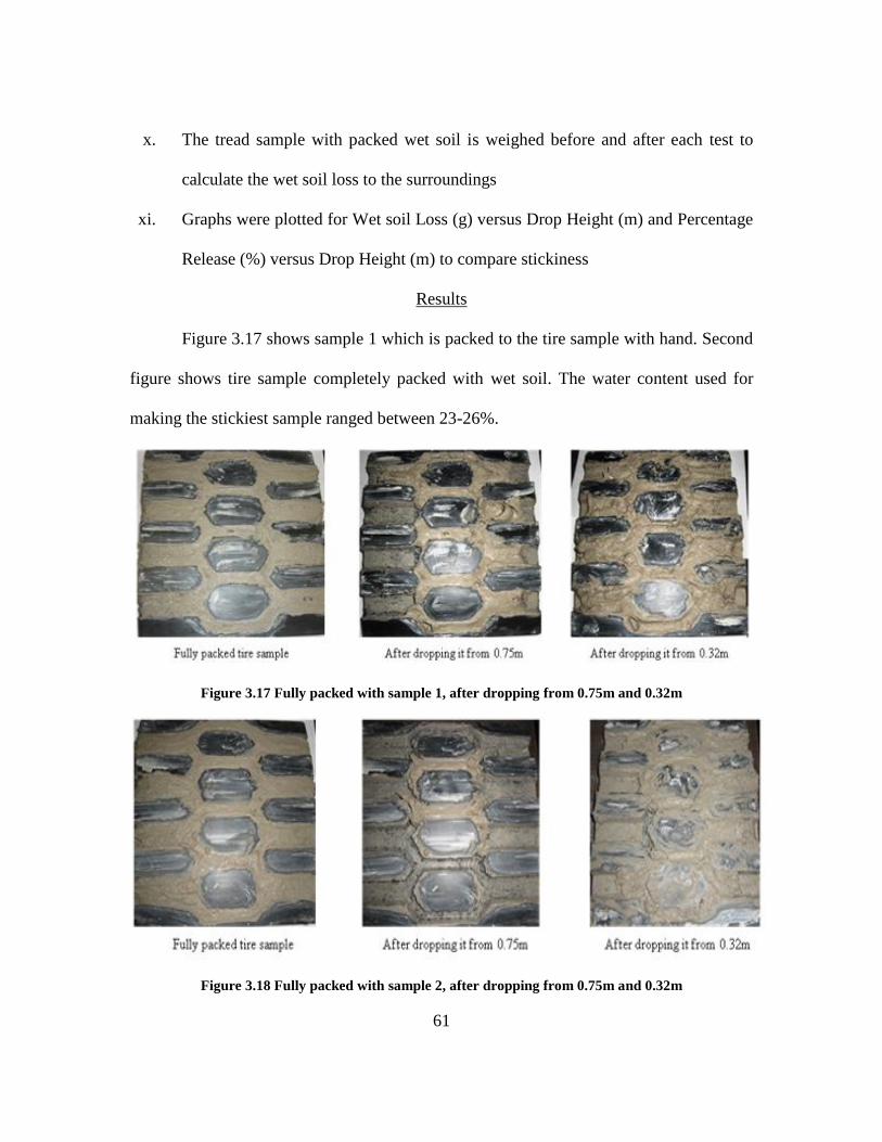
61

x. The tread sample with packed wet soil is weighed before and after each test to

calculate the wet soil loss to the surroundings

xi. Graphs were plotted for Wet soil Loss (g) versus Drop Height (m) and Percentage

Release (%) versus Drop Height (m) to compare stickiness

Results

Figure 3.17 shows sample 1 which is packed to the tire sample with hand. Second

figure shows tire sample completely packed with wet soil. The water content used for

making the stickiest sample ranged between 23-26%.

Figure 3.17 Fully packed with sample 1, after dropping from 0.75m and 0.32m

Figure 3.18 Fully packed with sample 2, after dropping from 0.75m and 0.32m

62

Figure 3.19 Fully packed with sample 3, after dropping from 0.75m, 0.5m and 0.32m

From Figure 3.17, Figure 3.18 and Figure 3.19 it is obvious that the tire sample

cleans up better when dropped from 0.75m and there is least mass loss when dropped

from 0.32m. With increase in drop height, the mass loss also increased.

Therefore, it can be concluded that the wet soil in open channel or groove cleans

up quickly when compared to wet soil that is closely packed. In the figure, the end

grooves have an open channel and the middle grooves do not have. Hence, the end

grooves are completely clean when compared to middle grooves when dropped from

0.75m. Similar behavior is observed when dropped from 0.32m height also. It is observed

that the mass loss begins first at the end grooves and then continues to the middle

grooves.

63

From Figure 3.19, it can be seen that the water content is fairly high in the soil

sample and the wet soil looks soupy. When dropped from 0.75m it is almost completely

clean.

In Figure 3.17, the tire sample looks very clean and there is more mass loss when

compared to other samples. From this, it is concluded that sample 1 is stickier when

compared to other samples.

Table 3.7, Table 3.8 and Table 3.9shows that sample 1 has the least mass loss

across all three drop heights and therefore considered as the stickiest of the samples, and

significantly stickier than the potting soil.

Replication 1

Sample 1

Table 3.6 Replication 1 on drop apparatus with sample 1

Parameter Test 1 Test 2 Test 3

Drop Height(m) 0.75 0.50 0.32

Mass before drop(g) 1608.30 1604.40 1613.30

Mass after drop(g) 1496.60 1567.40 1600.20

Mass loss(g) 111.70 37.00 13.10

Packed wet soil mass (g) 487.30 483.40 492.30

Percentage Released (%) 22.92 7.65 2.66

Sample 2

Table 3.7 Replication 1 on drop apparatus with sample 2

Parameter Test 1 Test 2 Test 3

Drop Height(m) 0.75 0.50 0.32

Mass before drop(g) 1641.60 1624.90 1600.80

Mass after drop(g) 1206.90 1230.50 1390.30

64

Mass loss(g) 434.70 394.40 210.50

Packed wet soil mass (g) 520.60 503.90 479.80

Percentage Released (%) 83.50 78.27 43.87

Sample 3

Table 3.8 Replication 1 on drop apparatus using sample 3

Parameter Test 1 Test 2 Test 3

Drop Height(m) 0.75 0.50 0.32

Mass before drop(g) 1602.70 1578.90 1589.10

Mass after drop(g) 1199.40 1363.60 1436.10

Mass loss(g) 403.30 215.30 153.00

Packed wet soil mass (g) 481.70 457.90 468.10

Percentage Released (%) 83.72 47.02 32.69

Figure 3.20 shows a combined graph for three soil samples and potting with mass

loss on y-axis and drop height on x-axis for replication 1.

Figure 3.20 Mass loss versus drop height

65

Figure 3.21 Percentage soil release with drop height

Replication 2

The results from the second replication again show sample 1 as having the least

mass loss across all three drop heights and therefore being the stickiest of the samples,

and significantly stickier than the potting soil.

Figure 3.22 With drop height mass loss has increased

66

Sample 1

Table 3.9 Replication 2 on drop apparatus using sample 1

Parameter Test 1 Test 2 Test 3

Drop Height(m) 0.75 0.50 0.32

Mass before drop(g) 1604.70 1592.20 1598.50

Mass after drop(g) 1430.30 1523.80 1590.20

Mass loss(g) 174.40 68.40 8.30

Packed wet soil mass(g) 483.70 471.20 477.50

Percentage Released (%) 36.06 14.52 1.74

Sample 2

Table 3.10 Replication 2 on drop apparatus using sample 2

Parameter Test 1 Test 2 Test 3

Drop Height(m) 0.75 0.50 0.32

Mass before drop(g) 1640.30 1628.60 1608.30

Mass after drop(g) 1220.20 1318.80 1432.20

Mass loss(g) 420.10 309.80 176.10

Packed wet soil mass(g) 519.30 507.60 487.30

Percentage Released (%) 80.90 61.03 36.14

Sample 3

Table 3.11 Replication 2 on drop apparatus using sample 3

Parameter Test 1 Test 2 Test 3

Drop Height(m) 0.75 0.50 0.32

Mass before drop(g) 1608.40 1598.10 1598.60

Mass after drop(g) 1257.40 1366.80 1482.30

Mass loss(g) 351.00 231.30 116.30

Packed wet soil mass(g) 487.40 477.10 477.60

Percentage Released (%) 72.01 48.48 24.35

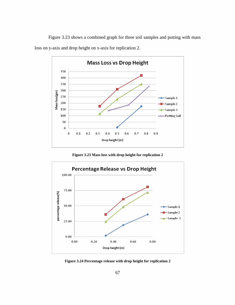
67

Figure 3.23 shows a combined graph for three soil samples and potting with mass

loss on y-axis and drop height on x-axis for replication 2.

Figure 3.23 Mass loss with drop height for replication 2

Figure 3.24 Percentage release with drop height for replication 2

68

Replication 3

In the third replication with soil composition, the water content was changed as

new batches of each of the samples had to be made. These new samples are named as

sample 4, sample 5, and sample 6. The change in water content has significant impact on

the results due to the subjectivity of the method for adding water to each sample. The

results from the third replication show a near tie between sample 1 and sample 3 in terms

of least wet soil lost. However from the graphs, both are and significantly stickier than

the potting soil.

Table 3.12 Samples considered for replication 3 on drop apparatus

Sample Clay (%) Silt (%) Sand (%) Water content (%)

4 35 20 45 29

5 20 15 65 25

6 20 20 60 31.2

Potting soil 57 19 24 32.5

Sample 4

Table 3.13 Replication 3 on drop apparatus using sample 4

Parameter Test 1 Test 2 Test 3

Drop Height(m) 0.75 0.50 0.25

Mass before drop(g) 1595.60 1598.70 1605.00

Mass after drop(g) 1535.30 1548.00 1603.00

Mass loss(g) 60.30 50.70 2.00

Packed wet soil mass (g) 474.60 477.70 484.00

Percentage Released (%) 12.71 10.61 0.41

69

Sample 5

Table 3.14 Replication 3 on drop apparatus with sample 5

Parameter Test 1 Test 2 Test 3

Drop Height(m) 0.75 0.50 0.25

Mass before drop(g) 1650.20 1630.50 1641.00

Mass after drop(g) 1394.30 1398.80 1502.20

Mass loss(g) 255.90 231.70 138.80

Packed wet soil mass (g) 529.20 509.50 520.00

Percentage Released (%) 48.36 45.48 26.69

Sample 6

Table 3.15 Replication 3 on drop apparatus using sample 6

Parameter Test 1 Test 2 Test 3

Drop Height(m) 0.75 0.50 0.25

Mass before drop(g) 1628.00 1609.60 1627.10

Mass after drop(g) 1541.30 1566.20 1624.20

Mass loss(g) 86.70 43.40 2.90

Packed wet soil mass (g) 507.00 488.60 506.10

Percentage Released (%) 17.10 8.88 0.57

Figure 3.25 shows a combined graph for soil samples and potting with mass loss

Figure 3.25 Mass loss vs drop height

70

Figure 3.26 Percentage release with drop height for replication 3

Figure 3.27 shows a graph for average wet soil loss (g) vs drop height (m) and

Figure 3.28 shows a graph for average percentage release (%) vs drop height (m) across

all three replications. Sample 1 is the stickiest mixture at the two highest drop heights.

Figure 3.27 Average mass loss with drop height

71

Figure 3.28 Average percentage loss with drop height

Discussion

The mass loss increases with the drop height as expected. This is obvious from

Figure 3.20, Figure 3.22 and Figure 3.25. From Figure 3.20, it is clear that the potting

soil line lies between the lines of customized wet soil samples. Potting soil was

considered to be not fairly sticky. Hence, the sample which lies below the potting soil can

be considered as sticky wet soil. Only sample-1 lies below the plot of potting soil in all

the three plots for mass loss vs. drop height. Therefore, it is the stickiest wet soil of all the

samples and sufficiently stickier than the potting soil mixture. Sample-1 has the highest

clay percentage which appears to be the reason for its high stickiness.

In Figure 3.20, two samples, sample-1 and sample-3 lie below the potting soil

line. Sample-3 in third replication has 31.2% water content whereas for the first 2

replications the water content used was 23.4%. Hence, water also plays a key role in

determining the stickiness of the wet soil mixtures.

72

Figure 3.21, Figure 3.24 and Figure 3.26 depicts the percentage release of wet soil

with different heights and it is again clear from these plots that with height the percentage

release of wet soil increases.

The sample-1 might be sticky either because of more clay content or water

content. Different mixtures of sand, silt and clay need different amounts of water for

making sticky wet soil. There is again no definite method for determining the water

content to make a sticky mixture.

These customized soil samples do not contain any organic matter and organic

matter is another factor which may contribute to the stickiness of the wet soil. Potting soil

had little amount of organic matter which contributed to the stickiness of potting soil.

3.3 CHAPTER SUMMARY

It can be concluded that sample-1 is stickier than the potting soil and all other

mixtures used in this experiment. The composition used for making sample 1 can

therefore be considered for future testing of the drop apparatus and the rotating arm

apparatus as a wet soil which is significantly stickier than the potting soil. Hence, the

adhesiveness of various samples is studied.

73

CHAPTER 4

4 SOIL BEHAVIOR MODELING – STRENGTH

The aim of this chapter is to develop a stress-strain model for a particular soil

composition to verify the changes in true stress and true strain with change in moisture

content. Assuming soil as strain hardening, a model is plotted. The purpose of this

chapter is to explain the soil compaction process and describe the assumed strain

hardening behavior of wet soils.

4.1 THEORETICAL STRESS STRAIN MODEL

In metals, strain hardening occurs when a material is strained beyond the

saturation point. Strain hardening is caused by plastic deformation where the material

cannot pull back itself in the original shape. Under strain hardening, metals grow in

strength due to grain boundary interference. We assume on a physical level that a similar

process occurs in soil when individual particles begin to interfere with one another, and

expect that the level of interference increases with the strain.

An engineering stress-strain curve will not give us the accurate relationship as the

stress-strain values depend on the original dimensions of the test sample. Wet soil is a

fluid which is non-Newtonian in nature. For such fluids, the relation between shear stress

and strain rate is non-linear and it is also time dependent[47]

. The stress at any given

instance is called as true stress and can be expressed in terms of engineering stress;

Eqn.(4.17) gives the relationship. Therefore, an instantaneous measure of stress-strain

called as the true stress-true stain curve is required to study the permanent deformation as

shown in Figure 4.1.

74

For any strain hardening metal,

nK (4.16)

where,

σ is the true stress,

K is the strength coefficient, and

n is the strain hardening index.

Eqn.(4.17) gives the relationship between true stress and engineering stress

( 1)s e (4.17)

where,

σ is the true stress,

e is the engineering strain, and

s is the engineering stress.

Eqn.(4.18) gives the relation between true strain and engineering strain

ln( 1)e (4.18)

where, ε is the true strain.

The engineering strain is defined by

0

le

L

(4.19)

where,

L0 is original length and

∆l is the change in length (when a sample is subjected to elongation)

75

K is a constant and depends on the structure of a material and n ranges from 0 to

1. If a material is perfectly plastic, n=0 and if it is perfectly elastic, n=1. Generally, n

varies from 0.1 to 0.5 for metals (Figure 4.1).

Figure 4.1 Relation between true stress and true stain based on n value

Wet soil is assumed as a strain hardening material because, when force is applied

on a block of wet soil, grains within the block move closer by ejecting the air and

moisture from the voids. As a result of this, particles get very close to each other and

create a particle to particle contact. This reduction in voids is shown in Figure 4.2. When

wet soil is compressed air is ejected out of the voids and particles get closer to each other.

76

Figure 4.2 Reduction in void spaces[48]

77

4.2 SOIL STRENGTH MODEL FROM COMPACTION TEST

Under compaction, the area for the sample keeps increasing as it is an unconfined

test and hence the stress also varies. The sample that is considered for the previous

experiments i.e. the stickiest mixture of all is assumed to be strain hardening in nature.

Three different soil samples with moisture contents of 17%, 19% and 21% are tested

under compression.

4.2.1 Procedure

This test was carried out on a SATEC Apex Tabletop Testing system, T10000

model. Figure 4.3 shows the tensile testing machine that was used for soil compaction

test. The maximum load that can be applied using this machine is 500N. The tensile

testing machine was controlled using a computer which uses a software called Blue Hill

to control the machine, enter the inputs, and record various results. Soil sample is

compacted by applying a continuous load in the range 0-500N with the help of the

software. The true stress and true strain are recorded at various points with the help of

software. All the initial test conditions are entered using the software and the load is

applied automatically as soon as the process starts. Figure 4.4 shows the Blue hill

software interface where the soil sample dimensions such as initial height and weight,

loading conditions, and anvil height are mentioned. Care is taken not to apply the load

beyond 500N as the sensor may burn out.

78

Figure 4.3 Satec tensile testing machine

Figure 4.4 Blue hill software - inputs mentioned

79

4.2.2 Results

Schematic representation of soil under compaction is shown in Figure 4.5. As this

is an unconfined test, the wet soil keeps increasing in diameter and its width decreases,

which validates the true stress-strain representation.

Figure 4.5 Different stages in soil compaction test

80

Three samples are made for testing using similar dry soil proportions but varying

the moisture content for each sample. Composition for samples is shown in Table 4.1.

The study of moisture effect on true stress and true strain is also observed by applying

compaction on a wet soil sample. The graph for true stress-true strain is plotted with

values obtained from the test results. Considering true strain till 50%, the graphs plotted

show that wet soil is strain hardening till this point. For each, a model of the form (Eqn.

(4.20)) is fit using a least-squares technique.

Table 4.1 Sample Compositions

Sample Moisture Content

(%) Sand (%) Clay (%) Silt (%)

1 17 45 35 20

2 19 45 35 20

3 21 45 35 20

Sample 1

Figure 4.6 True stress-true strain model for sample with 17% water

81

Sample 2

Figure 4.7 True stress- true strain model for sample with 19% water

Sample 3

Figure 4.8 True stress - true strain model for sample with 20% water

82

Using solver and applying multivariable regression, K and n values are optimized

and when plotted gave a best fit model and hence, equations for K and n in terms of

moisture content is formulated. The results for K is shown in Figure 4.9 and for n in

Figure 4.10.

Figure 4.9 Plot of strength coefficient, K

Figure 4.10 Plot for strain hardening index,n

83

The fundamental equation for a strain hardening model is shown in Eqn. (4.20)

nK (4.20)

Figure 4.9 gives a relation for strength coefficient, K and moisture fraction, M and

is shown in Eqn.(4.21). The relation between strain hardening index, n and moisture

fraction M and is shown in Eqn.(4.22).

0.35 0.8K M (4.21)

1.52 3.5n M (4.22)

Here, M = moisture fraction in the order of 10-4

Hence, for a given moisture content, true stress is given by Eqn.(4.23).

(1.52 3.5 )(0.35 0.8 ) MM (4.23)

The constraints on this relationship are that the moisture content is between the

liquid limit and plastic limit which are determined by the Atterberg test, and that the true

strain cannot exceed 50%.

4.2.3 Classical Strain Hardening Model

When we compare the true stress-true strain results and results assuming wet soil

as a strain hardening material, it shows that below 50% strain, results follow the strain

hardening curve. Above 50% however, the curve deviates from the strain hardening

behavior. In this case, behavior can be accurately represented by a general polynomial

equation of the form

3 2

0 1 2 3a a a a (4.24)

This model is fit using a least-squares technique to the entire data set. Results for

17%, 19% and 21% moisture are as shown in Figure 4.6, Figure 4.7 and Figure 4.8.

84

Sample 1

Figure 4. 1 Polynomial model for sample with 17% moisture

Sample 2

Figure 4. 2 Polynomial model for sample with 19% moisture

85

Figure 4. 3 Polynomial model for sample with 21% moisture

Plots for a0, a1, a2, a3 versus moisture content

The plots best fit plots for a0, a1, a2 and a3 are as shown in Figure 4.11, Figure

4.12, Figure 4.13 and Figure 4.14.

Figure 4.11 Relation for a0 and moisture content

86

Figure 4.12 Relation for a1 and moisture content

Figure 4.13 Relation for a2 and moisture content

87

Figure 4.14 Relation for a3 and moisture content

The relation between a0, a1, a2, a3 and moisture content is as shown below:

7 5

0

18

1

2

3

5*10 2*10

1*10 0.001

0.021 0.005

0.017 0.3

a M

a M

a M

a M

(4.25)

Neglecting higher order terms, the generalized model equation is given as follows:

20.001 [0.01 ] 2 0.3M M (4.26)

M is moisture content added to a soil in the order of 10E-04.

4.3 CHAPTER SUMMARY

Model for soil strength is developed. Initially, stain hardening is assumed to relate

to the physics-based representation. The strain hardening representation follows the given

data till about 50%, but deviates at large strains. Therefore, a general polynomial model

88

is developed to explain the deviation. By utilizing this model, for any given moisture

content, strength coefficient and strain hardening index can be obtained.

89

CHAPTER 5

5 FORCE MODEL

To develop a force model which calculates the speed at which the wet soil flies

off of the tire, wet soil in a channel is considered. The wet soil in the channel is exposed

to air on one side (hence no force is acting), second side is attached to the adjacent wet

soil, the other two sides are in contact with the sidewalls of the tire. There is no shear

force acting due to the sidewalls, as the wet soil does not break but peels out of the

channel.

5.1 FORCE MODEL

The free body diagram for a wet soil element of side one inch is developed as

shown in Figure 5.1. The forces acting on the wet soil element are as represented in the

figure. The forces that act are the centripetal force that tries to pull the wet soil out of the

channel, which is resisted by the vacuum force at the surface of the tire.

Constant values for the element considered for the free body analysis are:

9 3

4 2

6 3

, 1.97*10 /

, 6.25*10

, 15.625*10

, 0.0308

, 0.4

Mud

MudChunk

MudChunk

MudChunk

Density kg m

Area A m

Volume V m

Mass m kg

Radius r m

90

Figure 5.1 Free body diagram for wet soil element in a channel

Here, element is rotated at radius, R on a wheel balancing machine to simulate the

effect of soil in a tire groove. Fsidewall is the force exerted on the wet soil by the side walls

for the tread sample. Fvacuum is the force due to the air pockets and which helps in the peel

of the wet soil from the surface of the tire. This imparts a centripetal force of the form

F=mrω2. Pressure sensors embedded in the tire tread (shown is Figure 5.2) are used to

measure the pressure, P exerted on the wet soil. When the tire tread with sensors is

pressed in the soil, a pressure of 1-3psi is recorded.

91

Figure 5.2 Pressure sensors fixed in a tread sample

Assuming FSidewall as negligible,

Creating a force balance equation,

2

0F

F mr

(4.27)

,F

AngularVelocitymr

(4.28)

F is calculated from the drop test which comes to 120.7N for the considered mass

of the wet soil.

Substituting the values in Eqn.(4.28), angular velocity comes to 99Hz. Converting

these to road speed of a tire with the same dimension as the test setup, the speed at which

wet soil should release is 22.7mph. It depends on the mass of wet soil flying off of the

tire.

92

5.2 VALIDATION USING ROTATING ARM TEST RESULTS

Rotating arm test is carried out on the rotating arm apparatus. The main parts of

this apparatus are tire balancer, motor, drive, balancing arm and an assembly to hold the

tire tread sample. A remote data logger is used for recording various data about the wet

soil fly off.

Tire tread sample is fully packed with wet soil by hand, and is fixed to an

assembly on the rotating arm. The whole assembly is run with the help of a tire balancing

machine. The motor is used to test the sample at a ramp speed profile. Results for ramp

up speed test are shown in Table 5.1.

Table 5.1 Rotated arm results

Time

(s)

Speed

(mph)

Force

(N)

Mass estimate

(g)

Accumulated mass

(g)

8.47 0 0

8.5 24.3 1787 38.4 38.4

8.77 24.5 1845 4.8 43.2

9.13 24.6 1927 4.8 48.0

9.27 24.7 1907 4.8 52.8

9.33 24.7 1989 76.7 129.5

9.37 24.7 1957 9.6 139.1

9.43 24.8 1851 14.4 153.5

9.47 24.8 1854 38.4 191.8

9.5 24.8 1904 19.2 211.0

9.53 24.8 1967 76.7 287.7

9.6 24.8 1981 9.6 297.3

9.7 24.8 1858 38.4 335.7

9.73 24.8 1899 48.0 383.6

9.77 24.8 1964 9.6 393.2

9.93 24.9 1867 4.8 398.0

10.17 24.9 1873 4.8 402.8

10.77 25 2035 4.8 407.6

93

Graph is plotted for mass lass (grams) versus speed (mph) and is shown in Figure

5.3, which gives the range of speed for wet soil fly off i.e. between 15.5 and 19mph.

Figure 5.3 Wet soil fly off graph

5.3 CHAPTER SUMMARY

A force model is developed for calculating the speed at which the wet soil flies

off of the tire tread sample. The rotating arm test is carried out to validate this force

model. In this test, the wet soil flew off of the tire tread sample between a speed range of

15 and 19mph. The range of speeds obtained from rotating arm test is 25% closer to the

speed calculated using the force model. Hence, rotating arm test results validate the soil

force model.

94

CHAPTER 6

6 CONCLUSIONS AND FUTURE RECOMMENDATIONS

6.1 CONCLUSIONS

The main conclusion of this research is that sample with composition 45% sand,

35% clay and 20% silt is found to be the stickier soil among the different compositions

used in this experiments. Soil characteristics are studied with the help of Geotechnical

Engineering method like Sieve Analysis, Hydrometer Analysis, and Atterberg limits

Analysis. This composition is stickier than off-the-shelf potting soil. Study of stickiness

due to moisture content is understood with the help of true stress-true strain curves. The

soil composition can be used by the automotive industries to test off-road tires in a

laboratory.

It is also proved that small tire samples can be tested under controlled conditions

in a laboratory. This research enabled the use of tire tread samples for testing rather than

a full tire.

Two models are developed: one for soil strength and the other for adhesion force.

Initially, assuming wet soil as strain hardening a model is developed for true stress versus

true stain. Applying statistical methods to this model resulted in obtaining relations for

strength coefficient and strain hardening index in terms of moisture content. This strength

model is in 50% accordance with the true stress-true strain curve (result of compaction

test). For the values that deviated from the strain hardening model, a polynomial model is

generated using the best fit method; A force model is developed for calculating the speed

at which the wet soil flies off of the tire tread sample. The rotating arm test is carried out

95

to validate this force model. The range of speeds obtained from rotating arm test is 25%

closer to the range of speeds calculated using the force model.

6.2 SCOPE FOR FUTURE WORK

More research has to be done to study the effect of organic matter on the

stickiness as different particle sizes of organic might have different impact on the

stickiness. The introduction of organic matter in to the soil sample is important as tires

are run on the fields which have all kinds of matter. For laboratory testing peat can be

used. For the quantitative study of variation in stickiness due to moisture content, tests

used by Geotechnical Engineering like impact test and slump test. Another important

factor for future research is to study the effect of temperature on the soil samples made in

the laboratory.

96

REFERENCES

1. Mud tire tests and reviews. July 9 2007 [cited July 13 2008]; Available from:

http://www.4wheeloffroad.com/techarticles/mud_tires_tested/index.html.

2. Pidwirny, M., Fundamentals of Physical Geography. Chapter 10: Introduction to

the Lithosphere.

3. Brewer, R. and J.R. Sleeman, Soil structure and fabric: their definition and

description. J. Soil Sci, 1960. 11: p. 172-85.

4. Bormann, H., Analysis of the suitability of the German soil texture classification

for the regional scale application of physical based hydrological model. Advances in

Geosciences, 2007. 11: p. 7-13.

5. Terzaghi, K. and R.B. Peck, 1948, Soil Mechanics in Engineering Practice: John

Wiley and Sons, New York.

6. Miller, R.W. and D.T. Gardiner, Soils in our environment. Eighth ed. 1995:

Prentice Hall Upper Saddle River, NJ.

7. Day, R.W., Soil testing manual : procedures, classification data, and sampling

practices. 2001, New York: McGraw-Hill.

8. Soil Mechanics Lecture Notes. [cited April 17 2008]; Weight-Volume

Relationships]. Available from: http://www.eng.fsu.edu/~tawfiq/soilmech/lecture.html.

9. Das, B.M., Principles of Geotechnical Engineering. 1990: Brooks Cole.

10. Day, R.W., Soil Testing Manual: Procedures, Classification Data, and Sampling

Practices. 2001: McGraw-Hill Professional.

11. Astm, D., 3282/AASHTO M 145. Practice for Classification of Soils and Soil-

Aggregate Mixtures for Highway Construction Purposes.

12. Soils, B.S., ASTM D 2487 Soil Classification Groups GW, GP, GM, SW, SP, and

SM or AASHTO M 145 Soil Classification Groups A-1, A-2-4, A-2-5, and A-3, or a

combination of these groups.

13. Casagrande, A., CLASSIFICATION AND IDENTIFICATION OF SOILS. A

History of Progress: Selected US Papers in Geotechnical Engineering, 2003.

14. Staff, S.S., Soil Survey Manual. USDA Handbook no. 18. US Government

Printing Office, Washington, DC, 1993.

97

15. [cited June 27 2008]; Available from:

www.homegrownorganic.co.uk/soil_care_m.htm.

16. Abu-Zreig, M.M., N.M. Al-Akhras, and M.F. Attom, Influence of heat treatment

on the behavior of clayey soils. Applied Clay Science, 2001. 20(3): p. 129-135.

17. Zhang, X., N.H. Younan, and R.L. King, Soil texture classification using wavelet

transform and maximum likelihood approach. Geoscience and Remote Sensing

Symposium, 2003. IGARSS'03. Proceedings. 2003 IEEE International, 2003. 4.

18. Sumner, M.E., Handbook of Soil Science. 2000: CRC Press.

19. Lambe, T.W. and R.V. Whitman, Soil Mechanics. 1969: Wiley.

20. Braja, M., Das “Principles of Geotechnical Engineering”. Brooks/Cole

Thompson, 2002: p. 113-114.

21. July 15 2004 [cited July 1 2008]; Available from:

http://soils.tfrec.wsu.edu/mg/physical.htm.

22. Baver, L.D., Soil Physics. 1956.

23. Shepherd, T.G., Visual soil assessment. Field Guide for Cropping and Pastoral

Grazing on Flat to Rolling Country, 2000. 1.

24. Dekker, L.W., Moisture variability resulting from water repellency in Dutch soils.

The Netherlands, 1998. 240 p, Doctoral Thesis). Wageningen Agricultural University.

25. Das. Soil Mechanics and Foundation. [cited June 30 2008]; Available from:

http://ecow.engr.wisc.edu/cgi-bin/getbig/ema/506/carpick/designproj/soil_chapter.pdf.

26. Gill, W.R. and G.E.V. Berg, Soil Dynamics in Tillage and Traction, Agricultural

Handbook No. 316. Agricultural Research Service, USDA Washington, DC: US

Government Printing Office, 1967.

27. Wang, X.L., et al., Study on use of vibration to reduce soil adhesion. Journal of

Terramechanics, 1998. 35(2): p. 87-101.

28. Zacharias, G., BASIC STUDIES ON ATTERBERG LIMITS. Indian Journal of

Technology, 1975. 13(6): p. 269-273.

29. Faas, R., Rheological boundaries of mud: Where are the limits? Geo-Marine

Letters, 1991. 11(3): p. 143-146.

98

30. Warrick, A.W., Soil physics companion. 2002: CRC Press, Boca Raton.

31. Gee, G.W. and M.E. Dodson, Soil Water Content by Microwave Drying: A

Routing Procedure. Soil Sci Soc Am J, 1981. 45(6): p. 1234-1237.

32. Smith, K.A. and C.E. Mullins, Soil and environmental analysis: physical

methods. 2001: Marcel Dekker, New York.

33. Tollner, E.W., Soil Dynamics. Encyclopedia of agricultural, food, and biological

engineering, 2003.

34. Terzaghi, K., et al., From theory to practice in soil mechanics selections from the

writings of Karl Terzaghi. Contact. 650: p. 926-2411.

35. Terzaghi, K., Theoretical Soil Mechanics. 1943: Wiley.

36. Li, X. and J.M. Moshell, Modeling soil: realtime dynamic models for soil

slippage and manipulation. Proceedings of the 20th annual conference on Computer

graphics and interactive techniques, 1993: p. 361-368.

37. Poulos, S.J., The Steady State of Deformation. Journal of the Geotechnical

Engineering Division, 1981. 107(5): p. 553-562.

38. Dekker, L.W. and C.J. Ritsema, Wetting patterns and moisture variability in

water repellent Dutch soils. Journal of Hydrology, 2000. 231-232: p. 148-164.

39. Keller, T., et al., SoilFlex: A model for prediction of soil stresses and soil

compaction due to agricultural field traffic including a synthesis of analytical approaches.

Soil and Tillage Research, 2007. 93(2): p. 391-411.

40. Head, H.H., Manual of Soil Laboratory Testing, Volume I, Soil Classification and

Compaction Testing. 1984, Pentech Press.

41. Das, B.M., Soil Mechanics Laboratory Manual: Engineering Press San Jose,

Calif.(USA).

42. J. Medzvieckas, D.S., V. Stragys. Soil Mechanics. 2004 [cited; Available from:

http://www.vgtu.lt/leidiniai/elektroniniai/Laboratory_testing.pdf.

43. Houskova, B. and L. Montanarella, European Soil Visual Assessment-Field

Guide. The 18th World Congress of Soil Science, 2006.

44. Braja, M., Das, Soil mechanics Laboratory Manual. 2002, Oxford University

Press.

99

45. [cited 2008 Feb 27]; Available from: www.unisanet.unisa.edu.au.

46. Lambe, T.W., Soil testing for engineers. 1951.

47. Astm, D., 4318-00, 2003 ASTM D 4318-00, Standard test methods for liquid

limit, plastic limit, and plasticity index of soils. Annual Book of ASTM Standards, 2003:

p. 582–595.