quantitative social science: an introduction - chapter one introduction · 2019-09-30 · january...
TRANSCRIPT

January 5, 2017 Time: 12:08pm Chapter1.tex
Chapter 1
Introduction
In God we trust; all others must bring data.— William Edwards Deming
Quantitative social science is an interdisciplinary field encompassing a large numberof disciplines, including economics, education, political science, public policy, psy-chology, and sociology. In quantitative social science research, scholars analyze datato understand and solve problems about society and human behavior. For example,researchers examine racial discrimination in the labor market, evaluate the impactof new curricula on students’ educational achievements, predict election outcomes,and analyze social media usage. Similar data-driven approaches have been takenup in other neighboring fields such as health, law, journalism, linguistics, and evenliterature. Because social scientists directly investigate a wide range of real-world issues,the results of their research have enormous potential to directly influence individualmembers of society, government policies, and business practices.
Over the last couple of decades, quantitative social science has flourished in avariety of areas at an astonishing speed. The number of academic journal articlesthat present empirical evidence from data analysis has soared. Outside academia,many organizations—including corporations, political campaigns, news media, andgovernment agencies—increasingly rely on data analysis in their decision-makingprocesses. Two transformative technological changes have driven this rapid growth ofquantitative social science. First, the Internet has greatly facilitated the data revolution,leading to a spike in the amount and diversity of available data. Information sharingmakes it possible for researchers and organizations to disseminate numerous data setsin digital form. Second, the computational revolution, in terms of both software andhardware, means that anyone can conduct data analysis using their personal computerand favorite data analysis software.
As a direct consequence of these technological changes, the sheer volume of dataavailable to quantitative social scientists has rapidly grown. In the past, researcherslargely relied upon data published by governmental agencies (e.g., censuses, electionoutcomes, and economic indicators) as well as a small number of data sets collectedby research groups (e.g., survey data from national election studies and hand-codeddata sets about war occurrence and democratic institutions). These data sets still
© Copyright, Princeton University Press. No part of this book may be distributed, posted, or reproduced in any form by digital or mechanical means without prior written permission of the publisher.
For general queries, contact [email protected]

January 5, 2017 Time: 12:08pm Chapter1.tex
2 Chapter 1: Introduction
play an important role in empirical analysis. However, the wide variety of newdata has significantly expanded the horizon of quantitative social science research.Researchers are designing and conducting randomized experiments and surveys ontheir own. Under pressure to increase transparency and accountability, governmentagencies are making more data publicly available online. For example, in the UnitedStates, anyone can download detailed data on campaign contributions and lobbyingactivities to their personal computers. In Nordic countries like Sweden, a wide rangeof registers, including income, tax, education, health, and workplace, are available foracademic research.
New data sets have emerged across diverse areas. Detailed data about consumertransactions are available through electronic purchasing records. International tradedata are collected at the product level between many pairs of countries over sev-eral decades. Militaries have also contributed to the data revolution. During theAfghanistan war in the 2000s, the United States and international forces gathereddata on the geo-location, timing, and types of insurgent attacks and conducted dataanalysis to guide counterinsurgency strategy. Similarly, governmental agencies andnongovernmental organizations collected data on civilian casualties from the war.Political campaigns use data analysis to devise votermobilization strategies by targetingcertain types of voters with carefully selected messages.
These data sets also come in varying forms. Quantitative social scientists areanalyzing digitized texts as data, including legislative bills, newspaper articles, andthe speeches of politicians. The availability of social media data through websites,blogs, tweets, SMS messaging, and Facebook has enabled social scientists to explorehow people interact with one another in the online sphere. Geographical informationsystem (GIS) data sets are also widespread. They enable researchers to analyze thelegislative redistricting process or civil conflict with attention paid to spatial loca-tion. Others have used satellite imagery data to measure the level of electrificationin rural areas of developing countries. While still rare, images, sounds, and evenvideos can be analyzed using quantitative methods for answering social sciencequestions.
Together with the revolution of information technology, the availability of suchabundant and diverse data means that anyone, from academics to practitioners, frombusiness analysts to policy makers, and from students to faculty, can make data-drivendiscoveries. In the past, only statisticians and other specialized professionals conducteddata analysis. Now, everyone can turn on their personal computer, download datafrom the Internet, and analyze them using their favorite software. This has led toincreased demands for accountability to demonstrate policy effectiveness. In order tosecure funding and increase legitimacy, for example, nongovernmental organizationsand governmental agencies must now demonstrate the efficacy of their policies andprograms through rigorous evaluation.
This shift towards greater transparency and data-driven discovery requires thatstudents in the social sciences learn how to analyze data, interpret the results, andeffectively communicate their empirical findings. Traditionally, introductory statisticscourses have focused on teaching students basic statistical concepts by having themconduct straightforward calculations with paper and pencil or, at best, a scientificcalculator. Although these concepts are still important and covered in this book, this
© Copyright, Princeton University Press. No part of this book may be distributed, posted, or reproduced in any form by digital or mechanical means without prior written permission of the publisher.
For general queries, contact [email protected]

January 5, 2017 Time: 12:08pm Chapter1.tex
1.1 Overview of the Book 3
traditional approach cannot meet the current demands of society. It is simply notsufficient to achieve “statistical literacy” by learning about common statistical conceptsand methods. Instead, all students in the social sciences should acquire basic dataanalysis skills so that they can exploit the ample opportunities to learn from data andmake contributions to society through data-driven discovery.
The belief that everyone should be able to analyze data is the main motivation forwriting this book. The book introduces the three elements of data analysis requiredfor quantitative social science research: research contexts, programming techniques,and statistical methods. Any of these elements in isolation is insufficient. Withoutresearch contexts, we cannot assess the credibility of assumptions required for dataanalysis and will not be able to understand what the empirical findings imply. Withoutprogramming techniques, we will not be able to analyze data and answer research ques-tions. Without the guidance of statistical principles, we cannot distinguish systematicpatterns, known as signals, from idiosyncratic ones, known as noise, possibly leadingto invalid inference. (Here, inference refers to drawing conclusions about unknownquantities based on observed data.) This book demonstrates the power of data analysisby combining these three elements.
1.1 Overview of the Book
This book is written for anyone who wishes to learn data analysis and statistics forthe first time. The target audience includes researchers, undergraduate and graduatestudents in social science and other fields, as well as practitioners and even ambitioushigh-school students. The book has no prerequisite other than some elementaryalgebra. In particular, readers do not have to possess knowledge of calculus orprobability. No programming experience is necessary, though it can certainly behelpful. The book is also appropriate for those who have taken a traditional “paper-and-pencil” introductory statistics course where little data analysis is taught. Throughthis book, students will discover the excitement that data analysis brings. Those whowant to learn R programming might also find this book useful, although here theemphasis is on how to use R to answer quantitative social science questions.
As mentioned above, the unique feature of this book is the presentation of pro-gramming techniques and statistical concepts simultaneously through analysis of datasets taken directly from published quantitative social science research. The goal isto demonstrate how social scientists use data analysis to answer important questionsabout societal problems and human behavior. At the same time, users of the book willlearn fundamental statistical concepts and basic programming skills. Most importantly,readers will gain experience with data analysis by examining approximately fortydata sets.
The book consists of eight chapters. The current introductory chapter explainshow to best utilize the book and presents a brief introduction to R, a popularopen-source statistical programming environment. R is freely available for downloadand runs on Macintosh, Windows, and Linux computers. Readers are strongly en-couraged to use RStudio, another freely available software package that has numerousfeatures to make data analysis easier. This chapter ends with two exercises that are
© Copyright, Princeton University Press. No part of this book may be distributed, posted, or reproduced in any form by digital or mechanical means without prior written permission of the publisher.
For general queries, contact [email protected]

January 5, 2017 Time: 12:08pm Chapter1.tex
4 Chapter 1: Introduction
designed to help readers practice elementary R functionalities using data sets frompublished social science research. All data sets used in this book are freely available fordownload via links from http://press.princeton.edu/qss/. Links to otheruseful materials, such as the review exercises for each chapter, can also be found onthe website. With the exception of chapter 5, the book focuses on the most basicsyntax of R and does not introduce the wide range of additional packages that areavailable. However, upon completion of this book, readers will have acquired enoughR programming skills to be able to utilize these packages.
Chapter 2 introduces causality, which plays an essential role in social scienceresearch whenever we wish to find out whether a particular policy or program changesan outcome of interest. Causality is notoriously difficult to study because we must infercounterfactual outcomes that are not observable. For example, in order to understandthe existence of racial discrimination in the labor market, we need to know whether anAfrican-American candidate who did not receive a job offer would have done so if theywere white. We will analyze the data from a well-known experimental study in whichresearchers sent the résumés of fictitious job applicants to potential employers afterrandomly choosing applicants’ names to sound either African-American or Caucasian.Using this study as an application, the chapter will explain how the randomizationof treatment assignment enables researchers to identify the average causal effect ofthe treatment.
Additionally, readers will learn about causal inference in observational studies whereresearchers do not have control over treatment assignment. The main application is aclassic study whose goal was to figure out the impact of increasing the minimum wageon employment. Many economists argue that a minimum-wage increase can reduceemployment because employers must pay higher wages to their workers and are there-fore made to hire fewer workers. Unfortunately, the decision to increase the minimumwage is not random, but instead is subject to many factors, like economic growth,that are themselves associated with employment. Since these factors influence whichcompanies find themselves in the treatment group, a simple comparison between thosewho received treatment and those who did not can lead to biased inference.
We introduce several strategies that attempt to reduce this type of selection biasin observational studies. Despite the risk that we will inaccurately estimate treatmenteffects in observational studies, the results of such studies are often easier to generalizethan those obtained from randomized controlled trials. Other examples in chapter 2include a field experiment concerning social pressure in get-out-the-vote mobilization.Exercises then include a randomized experiment that investigates the causal effectof small class size in early education as well as a natural experiment about politicalleader assassination and its effects. In terms of R programming, chapter 2 covers logicalstatements and subsetting.
Chapter 3 introduces the fundamental concept of measurement. Accurate mea-surement is important for any data-driven discovery because bias in measurementcan lead to incorrect conclusions and misguided decisions. We begin by consideringhow to measure public opinion through sample surveys. We analyze the data from astudy in which researchers attempted to measure the degree of support among Afghancitizens for international forces and the Taliban insurgency during the Afghanistanwar. The chapter explains the power of randomization in survey sampling. Specifically,
© Copyright, Princeton University Press. No part of this book may be distributed, posted, or reproduced in any form by digital or mechanical means without prior written permission of the publisher.
For general queries, contact [email protected]
January 5, 2017 Time: 12:08pm Chapter1.tex
1.1 Overview of the Book 5
random sampling of respondents from a population allows us to obtain a representativesample. As a result, we can infer the opinion of an entire population by analyzing onesmall representative group. We also discuss the potential biases of survey sampling.Nonresponses can compromise the representativeness of a sample. Misreporting posesa serious threat to inference, especially when respondents are asked sensitive questions,such as whether they support the Taliban insurgency.
The second half of chapter 3 focuses on the measurement of latent or unobservableconcepts that play a key role in quantitative social science. Prominent examples of suchconcepts include ability and ideology. In the chapter, we study political ideology. Wefirst describe a model frequently used to infer the ideological positions of legislatorsfrom roll call votes, and examine how the US Congress has polarized over time. Wethen introduce a basic clustering algorithm, k-means, that makes it possible for us tofind groups of similar observations. Applying this algorithm to the data, we find that inrecent years, the ideological division within Congress has been mainly characterized bythe party line. In contrast, we find some divisions within each party in earlier years. Thischapter also introduces various measures of the spread of data, including quantiles,standard deviation, and the Gini coefficient. In terms of R programming, the chapterintroduces various ways to visualize univariate and bivariate data. The exercises includethe reanalysis of a controversial same-sex marriage experiment, which raises issues ofacademic integrity while illustrating methods covered in the chapter.
Chapter 4 considers prediction. Predicting the occurrence of certain events isan essential component of policy and decision-making processes. For example, theforecasting of economic performance is critical for fiscal planning, and early warningsof civil unrest allow foreign policy makers to act proactively. The main application ofthis chapter is the prediction of US presidential elections using preelection polls. Weshow that we can make a remarkably accurate prediction by combining multiple pollsin a straightforward manner. In addition, we analyze the data from a psychologicalexperiment in which subjects are shown the facial pictures of unknown politicalcandidates and asked to rate their competence. The analysis yields the surprising resultthat a quick facial impression can predict election outcomes. Through this example,we introduce linear regression models, which are useful tools to predict the values ofone variable based on another variable. We describe the relationship between linearregression and correlation, and examine the phenomenon called “regression towardsthe mean,” which is the origin of the term “regression.”
Chapter 4 also discusses when regression models can be used to estimate causaleffects rather than simply make predictions. Causal inference differs from standardprediction in requiring the prediction of counterfactual, rather than observed, out-comes using the treatment variable as the predictor. We analyze the data from arandomized natural experiment in India where randomly selected villages reservedsome of the seats in their village councils for women. Exploiting this randomization, weinvestigate whether or not having female politicians affects policy outcomes, especiallyconcerning the policy issues female voters care about. The chapter also introducesthe regression discontinuity design for making causal inference in observationalstudies. We investigate how much of British politicians’ accumulated wealth is dueto holding political office. We answer this question by comparing those who barelywon an election with those who narrowly lost it. The chapter introduces powerful but
© Copyright, Princeton University Press. No part of this book may be distributed, posted, or reproduced in any form by digital or mechanical means without prior written permission of the publisher.
For general queries, contact [email protected]

January 5, 2017 Time: 12:08pm Chapter1.tex
6 Chapter 1: Introduction
challenging R programming concepts: loops and conditional statements. The exercisesat the end of the chapter include an analysis of whether betting markets can preciselyforecast election outcomes.
Chapter 5 is about the discovery of patterns from data of various types. Whenanalyzing “big data,” we need automated methods and visualization tools to iden-tify consistent patterns in the data. First, we analyze texts as data. Our primaryapplication here is authorship prediction of The Federalist Papers, which formedthe basis of the US Constitution. Some of the papers have known authors whileothers do not. We show that by analyzing the frequencies of certain words in thepapers with known authorship, we can predict whether Alexander Hamilton orJames Madison authored each of the papers with unknown authorship. Second, weshow how to analyze network data, focusing on explaining the relationships amongunits. Within marriage networks in Renaissance Florence, we quantify the key roleplayed by the Medici family. As a more contemporary example, various measures ofcentrality are introduced and applied to social media data generated by US senatorson Twitter.
Finally in chapter 5, we introduce geo-spatial data. We begin by discussing theclassic spatial data analysis conducted by John Snow to examine the cause of the1854 cholera outbreak in London. We then demonstrate how to visualize spatial datathrough the creation of maps, using US election data as an example. For spatial–temporal data, we create a series of maps as an animation in order to visuallycharacterize changes in spatial patterns over time. Thus, the chapter applies variousdata visualization techniques using several specialized R packages.
Chapter 6 shifts the focus from data analysis to probability, a unified mathematicalmodel of uncertainty. While earlier chapters examine how to estimate parameters andmake predictions, they do not discuss the level of uncertainty in empirical findings, atopic that chapter 7 introduces. Probability is important because it lays a foundationfor statistical inference, the goal of which is to quantify inferential uncertainty. Webegin by discussing the question of how to interpret probability from two dominantperspectives, frequentist and Bayesian. We then provide mathematical definitions ofprobability and conditional probability, and introduce several fundamental rules ofprobability. One such rule is called Bayes’ rule. We show how to use Bayes’ rule andaccurately predict individual ethnicity using surname and residence location when nosurvey data are available.
This chapter also introduces the important concepts of random variables andprobability distributions.We use these tools to add ameasure of uncertainty to electionpredictions that we produced in chapter 4 using preelection polls. Another exerciseadds uncertainty to the forecasts of election outcomes based on betting market data.The chapter concludes by introducing two fundamental theorems of probability: thelaw of large numbers and the central limit theorem. These two theorems are widelyapplicable and help characterize how our estimates behave over repeated samplingas sample size increases. The final set of exercises then addresses two problems: theGerman cryptography machine from World War II (Enigma), and the detection ofelection fraud in Russia.
Chapter 7 discusses how to quantify the uncertainty of our estimates and pre-dictions. In earlier chapters, we introduced various data analysis methods to find
© Copyright, Princeton University Press. No part of this book may be distributed, posted, or reproduced in any form by digital or mechanical means without prior written permission of the publisher.
For general queries, contact [email protected]

January 5, 2017 Time: 12:08pm Chapter1.tex
1.2 How to Use this Book 7
patterns in data. Building on the groundwork laid in chapter 6, chapter 7 thoroughlyexplains how certain we should be about such patterns. This chapter shows howto distinguish signals from noise through the computation of standard errors andconfidence intervals as well as the use of hypothesis testing. In other words, the chapterconcerns statistical inference. Our examples come from earlier chapters, and we focuson measuring the uncertainty of these previously computed estimates. They includethe analysis of preelection polls, randomized experiments concerning the effects ofclass size in early education on students’ performance, and an observational studyassessing the effects of a minimum-wage increase on employment. When discussingstatistical hypothesis tests, we also draw attention to the dangers of multiple testing andpublication bias. Finally, we discuss how to quantify the level of uncertainty about theestimates derived from a linear regression model. To do this, we revisit the randomizednatural experiment of female politicians in India and the regression discontinuitydesign for estimating the amount of wealth British politicians are able to accumulateby holding political office.
The final chapter concludes by briefly describing the next steps readers might takeupon completion of this book. The chapter also discusses the role of data analysis inquantitative social science research.
1.2 How to Use this Book
In this section, we explain how to use this book, which is based on the followingprinciple:
One can learn data analysis only by doing, not by reading.
This book is not just for reading. The emphasis must be placed on gaining experiencein analyzing data. This is best accomplished by trying out the code in the book on one’sown, playing with it, and working on various exercises that appear at the end of eachchapter. All code and data sets used in the book are freely available for download vialinks from http://press.princeton.edu/qss/.
The book is cumulative. Later chapters assume that readers are already familiar withmost of the materials covered in earlier parts. Hence, in general, it is not advisableto skip chapters. The exception is chapter 5, “Discovery,” the contents of which arenot used in subsequent chapters. Nevertheless, this chapter contains some of themost interesting data analysis examples of the book and readers are encouraged tostudy it.
The book can be used for course instruction in a variety of ways. In a traditionalintroductory statistics course, one can assign the book, or parts of it, as supplementaryreading that provides data analysis exercises. The book is best utilized in a data analysiscourse where an instructor spends less time on lecturing to students and instead worksinteractively with students on data analysis exercises in the classroom. In such a course,the relevant portion of the book is assigned prior to each class. In the classroom, theinstructor reviews new methodological and programming concepts and then appliesthem to one of the exercises from the book or any other similar application of theirchoice. Throughout this process, the instructor can discuss the exercises interactively
© Copyright, Princeton University Press. No part of this book may be distributed, posted, or reproduced in any form by digital or mechanical means without prior written permission of the publisher.
For general queries, contact [email protected]

January 5, 2017 Time: 12:08pm Chapter1.tex
8 Chapter 1: Introduction
with students, perhaps using the Socratic method, until the class collectively arrivesat a solution. After such a classroom discussion, it would be ideal to follow up with acomputer lab session, in which a small number of students, together with an instructor,work on another exercise.
This teaching format is consistent with the “particular general particular” principle.1This principle states that an instructor should first introduce a particular example toillustrate a new concept, then provide a general treatment of it, and finally apply it toanother particular example. Reading assignments introduce a particular example and ageneral discussion of new concepts to students. Classroom discussion then allows theinstructor to provide another general treatment of these concepts and then, togetherwith students, apply them to another example. This is an effective teaching strategy thatengages students with active learning and builds their ability to conduct data analysisin social science research. Finally, the instructor can assign another application as aproblem set to assess whether students have mastered the materials. To facilitate this,for each chapter instructors can obtain, upon request, access to a private repository thatcontains additional exercises and their solutions.
In terms of the materials to cover, an example of the course outline for a15-week-long semester is given below. We assume that there are approximately twohours of lectures and one hour of computer lab sessions each week. Having hands-oncomputer lab sessions with a small number of students, in which they learn how toanalyze data, is essential.
Chapter title Chapter number WeeksIntroduction 1 1Causality 2 2–3Measurement 3 4–5Prediction 4 6–7Discovery 5 8–9Probability 6 10–12Uncertainty 7 13–15
For a shorter course, there are at least two ways to reduce the material. One option isto focus on aspects of data science and omit statistical inference. Specifically, from theabove outline, we can remove chapter 6, “Probability,” and chapter 7, “Uncertainty.”An alternative approach is to skip chapter 5, “Discovery,” which covers the analysisof textual, network, and spatial data, and include the chapters on probability anduncertainty.
Finally, to ensure mastery of the basic methodological and programming conceptsintroduced in each chapter, we recommend that users first read a chapter, practice allof the code it contains, and upon completion of each chapter, try the online reviewquestions before attempting to solve the associated exercises. These review questions
1 Frederick Mosteller (1980) “Classroom and platform performance.” American Statistician, vol. 34, no. 1(February), pp. 11–17.
© Copyright, Princeton University Press. No part of this book may be distributed, posted, or reproduced in any form by digital or mechanical means without prior written permission of the publisher.
For general queries, contact [email protected]

January 5, 2017 Time: 12:08pm Chapter1.tex
1.2 How to Use this Book 9
Table 1.1. The swirl Review Exercises.
Chapter swirl lesson Sections covered
1: IntroductionINTRO1 1.3INTRO2 1.3
2: CausalityCAUSALITY1 2.1–2.4CAUSALITY2 2.5–2.6
3: MeasurementMEASUREMENT1 3.1–3.4MEASUREMENT2 3.5–3.7
4: PredictionPREDICTION1 4.1PREDICTION2 4.2PREDICTION3 4.3
5: DiscoveryDISCOVERY1 5.1DISCOVERY2 5.2DISCOVERY3 5.3
6: ProbabilityPROBABILITY1 6.1–6.3PROBABILITY2 6.4–6.5
7: UncertaintyUNCERTAINTY1 7.1UNCERTAINTY2 7.2UNCERTAINTY3 7.3
Note: The table shows the correspondence between the chapters and sections ofthe book and each set of swirl review exercises.
are available as swirl lessons via links from http://press.princeton.edu/qss/, and can be answered within R. Instructors are strongly encouraged to assignthese swirl exercises prior to each class so that students learn the basics before movingon to more complicated data analysis exercises. To start the online review questions,users must first install the swirl package (see section 1.3.7) and then the lessons for thisbook using the following three lines of commands within R. Note that this installationneeds to be done only once.
install.packages("swirl") # install the package
library(swirl) # load the package
install_course_github("kosukeimai", "qss-swirl") # install the course
Table 1.1 lists the available set of swirl review exercises along with their correspond-ing chapters and sections. To start a swirl lesson for review questions, we can use thefollowing command.
library(swirl)
swirl()
More information about swirl is available at http://swirlstats.com/.
© Copyright, Princeton University Press. No part of this book may be distributed, posted, or reproduced in any form by digital or mechanical means without prior written permission of the publisher.
For general queries, contact [email protected]

January 5, 2017 Time: 12:08pm Chapter1.tex
10 Chapter 1: Introduction
1.3 Introduction to R
This section provides a brief, self-contained introduction to R that is a prerequisitefor the remainder of this book. R is an open-source statistical programming environ-ment, which means that anyone can download it for free, examine source code, andmake their own contributions. R is powerful and flexible, enabling us to handle a varietyof data sets and create appealing graphics. For this reason, it is widely used in academiaand industry. The New York Times described R as
a popular programming language used by a growing number of data analystsinside corporations and academia. It is becoming their lingua franca. . .whetherbeing used to set ad prices, find new drugs more quickly or fine-tune financialmodels. Companies as diverse as Google, Pfizer, Merck, Bank of America, theInterContinental Hotels Group and Shell use it. . . . “The great beauty of R is thatyou can modify it to do all sorts of things,” said Hal Varian, chief economist atGoogle. “And you have a lot of prepackaged stuff that’s already available, soyou’re standing on the shoulders of giants.”2
To obtain R, visit https://cran.r-project.org/ (The Comprehensive RArchive Network or CRAN), select the link that matches your operating system, andthen follow the installation instructions.
While a powerful tool for data analysis, R’s main cost from a practical viewpointis that it must be learned as a programming language. This means that we mustmaster various syntaxes and basic rules of computer programming. Learning computerprogramming is like becoming proficient in a foreign language. It requires a lot ofpractice and patience, and the learning process may be frustrating. Through numerousdata analysis exercises, this book will teach you the basics of statistical programming,which then will allow you to conduct data analysis on your own. The core principle ofthe book is that we can learn data analysis only by analyzing data.
Unless you have prior programming experience (or have a preference for anothertext editor such as Emacs), we recommend that you use RStudio. RStudio is an open-source and free program that greatly facilitates the use of R. In one window, RStudiogives users a text editor to write programs, a graph viewer that displays the graphicswe create, the R console where programs are executed, a help section, and manyother features. It may look complicated at first, but RStudio can make learning howto use R much easier. To obtain RStudio, visit http://www.rstudio.com/ andfollow the download and installation instructions. Figure 1.1 shows a screenshot ofRStudio.
In the remainder of this section, we cover three topics: (1) using R as a calculator,(2) creating and manipulating various objects in R, and (3) loading data sets into R.
1.3.1 ARITHMETIC OPERATIONSWe begin by using R as a calculator with standard arithmetic operators. In figure 1.1,
the left-hand window of RStudio shows the R console where we can directly enter R
2 Vance, Ashlee. 2009. “Data Analysts Captivated by R’s Power.” New York Times, January 6.
© Copyright, Princeton University Press. No part of this book may be distributed, posted, or reproduced in any form by digital or mechanical means without prior written permission of the publisher.
For general queries, contact [email protected]
January 5, 2017 Time: 12:08pm Chapter1.tex
1.3 Introduction to R 11
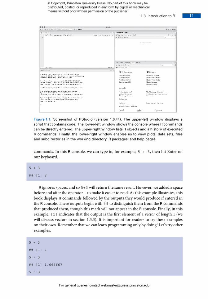
Figure 1.1. Screenshot of RStudio (version 1.0.44). The upper-left window displays ascript that contains code. The lower-left window shows the console where R commandscan be directly entered. The upper-right window lists R objects and a history of executedR commands. Finally, the lower-right window enables us to view plots, data sets, filesand subdirectories in the working directory, R packages, and help pages.
commands. In this R console, we can type in, for example, 5 + 3, then hit Enter onour keyboard.
5 + 3
## [1] 8
R ignores spaces, and so 5+3 will return the same result. However, we added a spacebefore and after the operator + to make it easier to read. As this example illustrates, thisbook displays R commands followed by the outputs they would produce if entered inthe R console. These outputs begin with ## to distinguish them from the R commandsthat produced them, though this mark will not appear in the R console. Finally, in thisexample, [1] indicates that the output is the first element of a vector of length 1 (wewill discuss vectors in section 1.3.3). It is important for readers to try these exampleson their own. Remember that we can learn programming only by doing! Let’s try otherexamples.
5 - 3
## [1] 2
5 / 3
## [1] 1.666667
5 ^ 3
© Copyright, Princeton University Press. No part of this book may be distributed, posted, or reproduced in any form by digital or mechanical means without prior written permission of the publisher.
For general queries, contact [email protected]
January 5, 2017 Time: 12:08pm Chapter1.tex
12 Chapter 1: Introduction
## [1] 125
5 * (10 - 3)
## [1] 35
sqrt(4)
## [1] 2
The final expression is an example of a so-called function, which takes an input(or multiple inputs) and produces an output. Here, the function sqrt() takes anonnegative number and returns its square root. As discussed in section 1.3.4, R hasnumerous other functions, and users can even make their own functions.
1.3.2 OBJECTSR can store information as an object with a name of our choice. Once we have created
an object, we just refer to it by name. That is, we are using objects as “shortcuts” tosome piece of information or data. For this reason, it is important to use an intuitiveand informative name. The name of our object must follow certain restrictions.For example, it cannot begin with a number (but it can contain numbers). Objectnames also should not contain spaces. We must avoid special characters such as %and $, which have specific meanings in R. In RStudio, in the upper-right window,called Environment (see figure 1.1), we will see the objects we created. We use theassignment operator <- to assign some value to an object.
For example, we can store the result of the above calculation as an object namedresult, and thereafter we can access the value by referring to the object’s name. Bydefault, Rwill print the value of the object to the console if we just enter the object nameand hit Enter. Alternatively, we can explicitly print it by using the print() function.
result <- 5 + 3
result
## [1] 8
print(result)
## [1] 8
Note that if we assign a different value to the same object name, then the value ofthe object will be changed. As a result, we must be careful not to overwrite previouslyassigned information that we plan to use later.
result <- 5 - 3
result
## [1] 2
© Copyright, Princeton University Press. No part of this book may be distributed, posted, or reproduced in any form by digital or mechanical means without prior written permission of the publisher.
For general queries, contact [email protected]

January 5, 2017 Time: 12:08pm Chapter1.tex
1.3 Introduction to R 13
Another thing to be careful about is that object names are case sensitive. Forexample, Hello is not the same as either hello or HELLO. As a consequence, wereceive an error in the R console when we type Result rather than result, which isdefined above.
Result
## Error in eval(expr, envir, enclos): object ‘Result’ not found
Encountering programming errors or bugs is part of the learning process. The trickypart is figuring out how to fix them. Here, the error message tells us that the Resultobject does not exist. We can see the list of existing objects in the Environmenttab in the upper-right window (see figure 1.1), where we will find that the correctobject is result. It is also possible to obtain the same list by using the ls()function.
So far, we have assigned only numbers to an object. But R can represent variousother types of values as objects. For example, we can store a string of characters byusing quotation marks.
kosuke <- "instructor"
kosuke
## [1] "instructor"
In character strings, spacing is allowed.
kosuke <- "instructor and author"
kosuke
## [1] "instructor and author"
Notice that R treats numbers like characters when we tell it to do so.
Result <- "5"
Result
## [1] "5"
However, arithmetic operations like addition and subtraction cannot be used forcharacter strings. For example, attempting to divide or take a square root of a characterstring will result in an error.
Result / 3
## Error in Result/3: non-numeric argument to binary operator
© Copyright, Princeton University Press. No part of this book may be distributed, posted, or reproduced in any form by digital or mechanical means without prior written permission of the publisher.
For general queries, contact [email protected]

January 5, 2017 Time: 12:08pm Chapter1.tex
14 Chapter 1: Introduction
sqrt(Result)
## Error in sqrt(Result): non-numeric argument to mathematical function
R recognizes different types of objects by assigning each object to a class. Separatingobjects into classes allows R to perform appropriate operations depending on theobjects’ class. For example, a number is stored as a numeric object whereas a characterstring is recognized as a character object. In RStudio, the Environment window willshow the class of an object as well as its name. The function (which by the way isanother class) class() tells us to which class an object belongs.
result
## [1] 2
class(result)
## [1] "numeric"
Result
## [1] "5"
class(Result)
## [1] "character"
class(sqrt)
## [1] "function"
There are many other classes in R, some of which will be introduced throughout thisbook. In fact, it is even possible to create our own object classes.
1.3.3 VECTORSWe present the simplest (but most inefficient) way of entering data into R. Table 1.2
contains estimates of world population (in thousands) over the past several decades.We can enter these data into R as a numeric vector object. A vector or a one-dimensional array simply represents a collection of information stored in a specificorder. We use the function c(), which stands for “concatenate,” to enter a data vectorcontaining multiple values with commas separating different elements of the vector weare creating. For example, we can enter the world population estimates as elements ofa single vector.
world.pop <- c(2525779, 3026003, 3691173, 4449049, 5320817, 6127700,
6916183)
world.pop
## [1] 2525779 3026003 3691173 4449049 5320817 6127700 6916183
© Copyright, Princeton University Press. No part of this book may be distributed, posted, or reproduced in any form by digital or mechanical means without prior written permission of the publisher.
For general queries, contact [email protected]

January 5, 2017 Time: 12:08pm Chapter1.tex
1.3 Introduction to R 15
Table 1.2. World Population Estimates.
YearWorld population
(thousands)1950 2,525,7791960 3,026,0031970 3,691,1731980 4,449,0491990 5,320,8172000 6,127,7002010 6,916,183Source: United Nations, Department
of Economic and Social Affairs, Popu-lation Division (2013). World PopulationProspects: The 2012 Revision, DVD Edition.
We also note that the c() function can be used to combine multiple vectors.
pop.first <- c(2525779, 3026003, 3691173)
pop.second <- c(4449049, 5320817, 6127700, 6916183)
pop.all <- c(pop.first, pop.second)
pop.all
## [1] 2525779 3026003 3691173 4449049 5320817 6127700 6916183
To access specific elements of a vector, we use square brackets [ ]. This is calledindexing. Multiple elements can be extracted via a vector of indices within squarebrackets. Also within square brackets the dash, -, removes the corresponding elementfrom a vector. Note that none of these operations change the original vector.
world.pop[2]
## [1] 3026003
world.pop[c(2, 4)]
## [1] 3026003 4449049
world.pop[c(4, 2)]
## [1] 4449049 3026003
world.pop[-3]
## [1] 2525779 3026003 4449049 5320817 6127700 6916183
Since each element of this vector is a numeric value, we can apply arithmeticoperations to it. The operations will be repeated for each element of the vector. Let’s
© Copyright, Princeton University Press. No part of this book may be distributed, posted, or reproduced in any form by digital or mechanical means without prior written permission of the publisher.
For general queries, contact [email protected]

January 5, 2017 Time: 12:08pm Chapter1.tex
16 Chapter 1: Introduction
give the population estimates inmillions instead of thousands by dividing each elementof the vector by 1000.
pop.million <- world.pop / 1000
pop.million
## [1] 2525.779 3026.003 3691.173 4449.049 5320.817 6127.700
## [7] 6916.183
We can also express each population estimate as a proportion of the 1950 populationestimate. Recall that the 1950 estimate is the first element of the vector world.pop.
pop.rate <- world.pop / world.pop[1]
pop.rate
## [1] 1.000000 1.198047 1.461400 1.761456 2.106604 2.426063
## [7] 2.738238
In addition, arithmetic operations can be done using multiple vectors. For example,we can calculate the percentage increase in population for each decade, defined as theincrease over the decade divided by its beginning population. For example, supposethat the population was 100 thousand in one year and increased to 120 thousand in thefollowing year. In this case, we say, “the population increased by 20%.” To compute thepercentage increase for each decade, we first create two vectors, one without the firstdecade and the other without the last decade. We then subtract the second vector fromthe first vector. Each element of the resulting vector equals the population increase. Forexample, the first element is the difference between the 1960 population estimate andthe 1950 estimate.
pop.increase <- world.pop[-1] - world.pop[-7]
percent.increase <- (pop.increase / world.pop[-7]) * 100
percent.increase
## [1] 19.80474 21.98180 20.53212 19.59448 15.16464 12.86752
Finally, we can also replace the values associated with particular indices by usingthe usual assignment operator (<-). Below, we replace the first two elements of thepercent.increase vector with their rounded values.
percent.increase[c(1, 2)] <- c(20, 22)
percent.increase
## [1] 20.00000 22.00000 20.53212 19.59448 15.16464 12.86752
1.3.4 FUNCTIONSFunctions are important objects in R and perform a wide range of tasks. A function
often takes multiple input objects and returns an output object. We have already seen
© Copyright, Princeton University Press. No part of this book may be distributed, posted, or reproduced in any form by digital or mechanical means without prior written permission of the publisher.
For general queries, contact [email protected]

January 5, 2017 Time: 12:08pm Chapter1.tex
1.3 Introduction to R 17
several functions: sqrt(), print(), class(), and c(). In R, a function generallyruns as funcname(input) where funcname is the function name and input isthe input object. In programming (and in math), we call these inputs arguments. Forexample, in the syntax sqrt(4), sqrt is the function name and 4 is the argument orthe input object.
Some basic functions useful for summarizing data include length() for thelength of a vector or equivalently the number of elements it has, min() forthe minimum value, max() for the maximum value, range() for the range ofdata, mean() for the mean, and sum() for the sum of the data. Right now weare inputting only one object into these functions so we will not use argumentnames.
length(world.pop)
## [1] 7
min(world.pop)
## [1] 2525779
max(world.pop)
## [1] 6916183
range(world.pop)
## [1] 2525779 6916183
mean(world.pop)
## [1] 4579529
sum(world.pop) / length(world.pop)
## [1] 4579529
The last expression gives another way of calculating the mean as the sum of all theelements divided by the number of elements.
When multiple arguments are given, the syntax looks like funcname(input1,input2). The order of inputs matters. That is, funcname(input1, input2) isdifferent from funcname(input2, input1). To avoid confusion and problemsstemming from the order in which we list arguments, it is also a good idea tospecify the name of the argument that each input corresponds to. This looks likefuncname(arg1 = input1, arg2 = input2).
For example, the seq() function can generate a vector composed of an increasingor decreasing sequence. The first argument from specifies the number to start from;the second argument to specifies the number at which to end the sequence; the lastargument by indicates the interval to increase or decrease by. We can create an objectfor the year variable from table 1.2 using this function.
© Copyright, Princeton University Press. No part of this book may be distributed, posted, or reproduced in any form by digital or mechanical means without prior written permission of the publisher.
For general queries, contact [email protected]

January 5, 2017 Time: 12:08pm Chapter1.tex
18 Chapter 1: Introduction
year <- seq(from = 1950, to = 2010, by = 10)
year
## [1] 1950 1960 1970 1980 1990 2000 2010
Notice how we can switch the order of the arguments without changing the outputbecause we have named the input objects.
seq(to = 2010, by = 10, from = 1950)
## [1] 1950 1960 1970 1980 1990 2000 2010
Although not relevant in this particular example, we can also create a decreasingsequence using the seq()function. In addition, the colon operator : creates a simplesequence, beginning with the first number specified and increasing or decreasing by 1to the last number specified.
seq(from = 2010, to = 1950, by = -10)
## [1] 2010 2000 1990 1980 1970 1960 1950
2008:2012
## [1] 2008 2009 2010 2011 2012
2012:2008
## [1] 2012 2011 2010 2009 2008
The names() function can access and assign names to elements of a vector.Element names are not part of the data themselves, but are helpful attributes of the Robject. Below, we see that the object world.pop does not yet have the names attribute,with names(world.pop) returning the NULL value. However, once we assign theyear as the labels for the object, each element of world.pop is printed with aninformative label.
names(world.pop)
## NULL
names(world.pop) <- year
names(world.pop)
## [1] "1950" "1960" "1970" "1980" "1990" "2000" "2010"
© Copyright, Princeton University Press. No part of this book may be distributed, posted, or reproduced in any form by digital or mechanical means without prior written permission of the publisher.
For general queries, contact [email protected]
January 5, 2017 Time: 12:08pm Chapter1.tex
1.3 Introduction to R 19
world.pop
## 1950 1960 1970 1980 1990 2000 2010
## 2525779 3026003 3691173 4449049 5320817 6127700 6916183
In many situations, we want to create our own functions and use them repeatedly.This allows us to avoid duplicating identical (or nearly identical) sets of code chunks,making our code more efficient and easily interpretable. The function() functioncan create a new function. The syntax takes the following form.
myfunction <- function(input1, input2, ..., inputN) {
DEFINE “output” USING INPUTS
return(output)
}
In this example code, myfunction is the function name, input1, input2,..., inputN are the input arguments, and the commands within the braces { }define the actual function. Finally, the return() function returns the output of thefunction. We begin with a simple example, creating a function to compute a summaryof a numeric vector.
my.summary <- function(x){ # function takes one input
s.out <- sum(x)
l.out <- length(x)
m.out <- s.out / l.out
out <- c(s.out, l.out, m.out) # define the output
names(out) <- c("sum", "length", "mean") # add labels
return(out) # end function by calling output
}
z <- 1:10
my.summary(z)
## sum length mean
## 55.0 10.0 5.5
my.summary(world.pop)
## sum length mean
## 32056704 7 4579529
Note that objects (e.g., x, s.out, l.out, m.out, and out in the above example)can be defined within a function independently of the environment in which thefunction is being created. This means that we need not worry about using identicalnames for objects inside a function and those outside it.
© Copyright, Princeton University Press. No part of this book may be distributed, posted, or reproduced in any form by digital or mechanical means without prior written permission of the publisher.
For general queries, contact [email protected]

January 5, 2017 Time: 12:08pm Chapter1.tex
20 Chapter 1: Introduction
1.3.5 DATA FILESSo far, the only data we have used has been manually entered into R. But, most of
the time, we will load data from an external file. In this book, we will use the followingtwo data file types:
• CSV or comma-separated values files represent tabular data. This is conceptuallysimilar to a spreadsheet of data values like those generated by Microsoft Excel orGoogle Spreadsheet. Each observation is separated by line breaks and each fieldwithin the observation is separated by a comma, a tab, or some other character orstring.
• RData files represent a collection of R objects including data sets. These cancontain multiple R objects of different kinds. They are useful for savingintermediate results from our R code as well as data files.
Before interacting with data files, we must ensure they reside in the working direc-tory, which R will by default load data from and save data to. There are different ways tochange the working directory. In RStudio, the default working directory is shown in thebottom-right window under the Files tab (see figure 1.1). Oftentimes, however, thedefault directory is not the directory we want to use. To change the working directory,click on More > Set As Working Directory after choosing the folder we wantto work from. Alternatively, we can use the RStudio pull-down menu Session >Set Working Directory > Choose Directory... and pick the folder wewant to work from. Then, we will see our files and folders in the bottom-right window.
It is also possible to change the working directory using the setwd() function byspecifying the full path to the folder of our choice as a character string. To display thecurrent working directory, use the function getwd() without providing an input. Forexample, the following syntax sets the working directory to qss/INTRO and confirmsthe result (we suppress the output here).
setwd("qss/INTRO")
getwd()
Suppose that the United Nations population data in table 1.2 are saved as a CSV fileUNpop.csv, which resembles that below:
year, world.pop1950, 25257791960, 30260031970, 36911731980, 44490491990, 53208172000, 61277002010, 6916183
In RStudio, we can read in or load CSV files by going to the drop-down menu in theupper-right window (see figure 1.1) and clicking Import Dataset > From Text
© Copyright, Princeton University Press. No part of this book may be distributed, posted, or reproduced in any form by digital or mechanical means without prior written permission of the publisher.
For general queries, contact [email protected]

January 5, 2017 Time: 12:08pm Chapter1.tex
1.3 Introduction to R 21
File .... Alternatively, we can use the read.csv() function. The following syntaxloads the data as a data frame object (more on this object below).
UNpop <- read.csv("UNpop.csv")
class(UNpop)
## [1] "data.frame"
On the other hand, if the same data set is saved as an object in an RData file namedUNpop.RData, then we can use the load() function, which will load all the R objectssaved in UNpop.RData into our R session. We do not need to use the assignmentoperator with the load() function when reading in an RData file because the R objectsstored in the file already have object names.
load("UNpop.RData")
Note that R can access any file on our computer if the full location is specified.For example, we can use syntax such as read.csv("Documents/qss/INTRO/UNpop.csv") if the data file UNpop.csv is stored in the directory Documents/qss/INTRO/. However, setting the working directory as shown above allows us toavoid tedious typing.
A data frame object is a collection of vectors, but we can think of it like a spreadsheet.It is often useful to visually inspect data. We can view a spreadsheet-like representationof data frame objects in RStudio by double-clicking on the object name in theEnvironment tab in the upper-right window (see figure 1.1). This will open a newtab displaying the data. Alternatively, we can use the View() function, which as itsmain argument takes the name of a data frame to be examined. Useful functions forthis object include names() to return a vector of variable names, nrow() to return thenumber of rows, ncol() to return the number of columns, dim() to combine the out-puts of ncol() and nrow() into a vector, and summary() to produce a summary.
names(UNpop)
## [1] "year" "world.pop"
nrow(UNpop)
## [1] 7
ncol(UNpop)
## [1] 2
dim(UNpop)
## [1] 7 2
© Copyright, Princeton University Press. No part of this book may be distributed, posted, or reproduced in any form by digital or mechanical means without prior written permission of the publisher.
For general queries, contact [email protected]

January 5, 2017 Time: 12:08pm Chapter1.tex
22 Chapter 1: Introduction
summary(UNpop)
## year world.pop
## Min. :1950 Min. :2525779
## 1st Qu.:1965 1st Qu.:3358588
## Median :1980 Median :4449049
## Mean :1980 Mean :4579529
## 3rd Qu.:1995 3rd Qu.:5724258
## Max. :2010 Max. :6916183
Notice that the summary() function yields, for each variable in the data frameobject, the minimum value, the first quartile (or 25th percentile), the median (or50th percentile), the third quartile (or 75th percentile), and the maximum value. Seesection 2.6 for more discussion.
The $ operator is one way to access an individual variable from within a data frameobject. It returns a vector containing the specified variable.
UNpop$world.pop
## [1] 2525779 3026003 3691173 4449049 5320817 6127700 6916183
Another way of retrieving individual variables is to use indexing inside squarebrackets[ ], as done for a vector. Since a data frame object is a two-dimensionalarray, we need two indexes, one for rows and the other for columns. Using bracketswith a comma [rows, columns] allows users to call specific rows and columns byeither row/column numbers or row/column names. If we use row/column numbers,sequencing functions covered above, i.e., : and c(), will be useful. If we do not specifya row (column) index, then the syntax will return all rows (columns). Below are someexamples, demonstrating the syntax of indexing.
UNpop[, "world.pop"] # extract the column called "world.pop"
## [1] 2525779 3026003 3691173 4449049 5320817 6127700 6916183
UNpop[c(1, 2, 3),] # extract the first three rows (and all columns)
## year world.pop
## 1 1950 2525779
## 2 1960 3026003
## 3 1970 3691173
UNpop[1:3, "year"] # extract the first three rows of the "year" column
## [1] 1950 1960 1970
© Copyright, Princeton University Press. No part of this book may be distributed, posted, or reproduced in any form by digital or mechanical means without prior written permission of the publisher.
For general queries, contact [email protected]

January 5, 2017 Time: 12:08pm Chapter1.tex
1.3 Introduction to R 23
When extracting specific observations from a variable in a data frame object, weprovide only one index since the variable is a vector.
## take elements 1, 3, 5, ... of the "world.pop" variable
UNpop$world.pop[seq(from = 1, to = nrow(UNpop), by = 2)]
## [1] 2525779 3691173 5320817 6916183
In R, missing values are represented by NA. When applied to an object with missingvalues, functions may or may not automatically remove those values before performingoperations. We will discuss the details of handling missing values in section 3.2. Here,we note that for many functions, like mean(), the argument na.rm = TRUE willremovemissing data before operations occur. In the example below, the eighth elementof the vector is missing, and one cannot calculate the mean until R has been instructedto remove the missing data.
world.pop <- c(UNpop$world.pop, NA)
world.pop
## [1] 2525779 3026003 3691173 4449049 5320817 6127700 6916183
## [8] NA
mean(world.pop)
## [1] NA
mean(world.pop, na.rm = TRUE)
## [1] 4579529
1.3.6 SAVING OBJECTSThe objects we create in an R session will be temporarily saved in the workspace,
which is the current working environment. As mentioned earlier, the ls()functiondisplays the names of all objects currently stored in the workspace. In RStudio, allobjects in the workspace appear in the Environment tab in the upper-right corner.However, these objects will be lost once we terminate the current session. This can beavoided if we save the workspace at the end of each session as an RData file.
When we quit R, we will be asked whether we would like to save the workspace. Weshould answer no to this so that we get into the habit of explicitly saving only whatwe need. If we answer yes, then R will save the entire workspace as .RData in theworking directory without an explicit file name and automatically load it next time welaunch R. This is not recommended practice, because the .RData file is invisible tousers of many operating systems and R will not tell us what objects are loaded unlesswe explicitly issue the ls() function.
In RStudio, we can save the workspace by clicking the Save icon in the upper-rightEnvironment window (see figure 1.1). Alternatively, from the navigation bar, click
© Copyright, Princeton University Press. No part of this book may be distributed, posted, or reproduced in any form by digital or mechanical means without prior written permission of the publisher.
For general queries, contact [email protected]

January 5, 2017 Time: 12:08pm Chapter1.tex
24 Chapter 1: Introduction
on Session > Save Workspace As..., and then pick a location to save the file.Be sure to use the file extension .RData. To load the same workspace the next time westart RStudio, click the Open File icon in the upper-right Environment window,select Session > Load Workspace..., or use the load() function as before.
It is also possible to save the workspace using the save.image() function. Thefile extension .RData should always be used at the end of the file name. Unless thefull path is specified, objects will be saved to the working directory. For example,the following syntax saves the workspace as Chapter1.RData in the qss/INTROdirectory provided that this directory already exists.
save.image("qss/INTRO/Chapter1.RData")
Sometimes, we wish to save only a specific object (e.g., a data frame object)rather than the entire workspace. This can be done with the save() functionas in save(xxx, file = "yyy.RData"), where xxx is the object name andyyy.RData is the file name. Multiple objects can be listed, and they will be storedas a single RData file. Here are some examples of syntax, in which we again assume theexistence of the qss/INTRO directory.
save(UNpop, file = "Chapter1.RData")
save(world.pop, year, file = "qss/INTRO/Chapter1.RData")
In other cases, we may want to save a data frame object as a CSV file rather than anRData file. We can use the write.csv() function by specifying the object name andthe file name, as the following example illustrates.
write.csv(UNpop, file = "UNpop.csv")
Finally, to access objects saved in the RData file, simply use the load() functionas before.
load("Chapter1.RData")
1.3.7 PACKAGESOne of R’s strengths is the existence of a large community of R users who con-
tribute various functionalities as R packages. These packages are available throughthe Comprehensive R Archive Network (CRAN; http://cran.r-project.org).Throughout the book, we will employ various packages. For the purpose of illustration,suppose that we wish to load a data file produced by another statistical software packagesuch as Stata or SPSS. The foreign package is useful when dealing with files from otherstatistical software.
© Copyright, Princeton University Press. No part of this book may be distributed, posted, or reproduced in any form by digital or mechanical means without prior written permission of the publisher.
For general queries, contact [email protected]

January 5, 2017 Time: 12:08pm Chapter1.tex
1.3 Introduction to R 25
To use the package, we must load it into the workspace using the library()function. In some cases, a package needs to be installed before being loaded. InRStudio, we can do this by clicking on Packages > Install in the bottom-right window (see figure 1.1), where all currently installed packages are listed, afterchoosing the desired packages to be installed. Alternatively, we can install from the Rconsole using the install.packages() function (the output is suppressed below).Package installation needs only to occur once, though we can update the packagelater upon the release of a new version (by clicking Update or reinstalling it via theinstall.packages() function).
install.packages("foreign") # install package
library("foreign") # load package
Once the package is loaded, we can use the appropriate functions to load the data file.For example, the read.dta() and read.spss() functions can read Stata and SPSSdata files, respectively (the following syntax assumes the existence of the UNpop.dtaand UNpop.sav files in the working directory).
read.dta("UNpop.dta")
read.spss("UNpop.sav")
As before, it is also possible to save a data frame object as a data file thatcan be directly loaded into another statistical software package. For example, thewrite.dta() function will save a data frame object as a Stata data file.
write.dta(UNpop, file = "UNpop.dta")
1.3.8 PROGRAMMING AND LEARNING TIPSWe conclude this brief introduction to R by providing several practical tips for
learning how to program in the R language. First, we should use a text editor like theone that comes with RStudio to write our program rather than directly typing it intothe R console. If we just want to see what a command does, or quickly calculate somequantity, we can go ahead and enter it directly into the R console. However, for moreinvolved programming, it is always better to use the text editor and save our code as atext file with the .R file extension. This way, we can keep a record of our program andrun it again whenever necessary.
In RStudio, use the pull-down menu File > New File > R Script or clickthe New File icon (a white square with a green circle enclosing a white plus sign)and choose R Script. Either approach will open a blank document for text editing inthe upper-left window where we can start writing our code (see figure 1.2). To run ourcode from the RStudio text editor, simply highlight the code and press the Run icon.Alternatively, inWindows, Ctrl+Enter works as a shortcut. The equivalent shortcut forMac is Command+Enter. Finally, we can also run the entire code in the background
© Copyright, Princeton University Press. No part of this book may be distributed, posted, or reproduced in any form by digital or mechanical means without prior written permission of the publisher.
For general queries, contact [email protected]

January 5, 2017 Time: 12:08pm Chapter1.tex
26 Chapter 1: Introduction
Figure 1.2. Screenshot of the RStudio Text Editor. Once we open an R script file inRStudio, the text editor will appear as one of the windows. It can then be used to writeour code.
(so, the code will not appear in the console) by clicking the Source icon or using thesource() function with the code file name (including a full path if it is not placed inthe working directory) as the input.
source("UNpop.R")
Second, we can annotate our R code so that it can be easily understandable toourselves and others. This is especially important as our code gets more complex. To dothis, we use the comment character #, which tells R to ignore everything that follows it.It is customary to use a double comment character ## if a comment occupies an entireline and use a single comment character # if a comment is made within a line after anR command. An example is given here.
##
## File: UNpop.R
## Author: Kosuke Imai
## The code loads the UN population data and saves it as a Stata file
##
library(foreign)
UNpop <- read.csv("UNpop.csv")
UNpop$world.pop <- UNpop$world.pop / 1000 # population in millions
write.dta(UNpop, file = "UNpop.dta")
© Copyright, Princeton University Press. No part of this book may be distributed, posted, or reproduced in any form by digital or mechanical means without prior written permission of the publisher.
For general queries, contact [email protected]

January 5, 2017 Time: 12:08pm Chapter1.tex
1.4 Summary 27
Third, for further clarity it is important to follow a certain set of coding rules.For example, we should use informative names for files, variables, and functions.Systematic spacing and indentation are essential too. In the above examples, we placespaces around all binary operators such as <-, =, +, and -, and always add a spaceafter a comma. While comprehensive coverage of coding style is beyond the scopeof this book, we encourage you to follow a useful R style guide published by Googleat https://google.github.io/styleguide/Rguide.xml. In addition, it ispossible to check our R code for potential errors and incorrect syntax. In computerscience, this process is called linting. The lintr() function in the lintr packageenables the linting of R code. The following syntax implements the linting of theUNpop.R file shown above, where we replace the assignment operator <- in line 8with the equality sign = for the sake of illustration.
library(lintr)
lint("UNpop.R")
## UNpop.R:8:7: style: Use <-, not =, for assignment.
## UNpop = read.csv("UNpop.csv")
## ^
Finally, R Markdown via the rmarkdown package is useful for quickly writingdocuments using R. R Markdown enables us to easily embed R code and its outputwithin a document using straightforward syntax in a plain-text format. The resultingdocuments can be produced in the form of HTML, PDF, or even Microsoft Word.Because R Markdown embeds R code as well as its output, the results of data analysispresented in documents are reproducible. R Markdown is also integrated into RStudio,making it possible to produce documents with a single click. For a quick start, seehttp://rmarkdown.rstudio.com/.
1.4 Summary
This chapter began with a discussion of the important role that quantitativesocial science research can play in today’s data-rich society. To make contributionsto this society through data-driven discovery, we must learn how to analyze data,interpret the results, and communicate our findings to others. To start our journey,we presented a brief introduction to R, which is a powerful programming language fordata analysis. The remaining pages of this chapter are dedicated to exercises, designedto ensure that you have mastered the contents of this section. Start with the swirlreview questions that are available via links from http://press.princeton.edu/qss/. If you answer these questions incorrectly, be sure to go backto the relevant sections and review the materials before moving on to theexercises.
© Copyright, Princeton University Press. No part of this book may be distributed, posted, or reproduced in any form by digital or mechanical means without prior written permission of the publisher.
For general queries, contact [email protected]

January 5, 2017 Time: 12:08pm Chapter1.tex
28 Chapter 1: Introduction
Table 1.3. US Election Turnout Data.
Variable Description
year election yearANES ANES estimated turnout rateVEP voting eligible population (in thousands)VAP voting age population (in thousands)total total ballots cast for highest office (in thousands)felons total ineligible felons (in thousands)noncitizens total noncitizens (in thousands)overseas total eligible overseas voters (in thousands)osvoters total ballots counted by overseas voters (in thousands)
1.5 Exercises
1.5.1 BIAS IN SELF-REPORTED TURNOUTSurveys are frequently used to measure political behavior such as voter turnout,
but some researchers are concerned about the accuracy of self-reports. In particular,they worry about possible social desirability bias where, in postelection surveys,respondents who did not vote in an election lie about not having voted because theymay feel that they should have voted. Is such a bias present in the American NationalElection Studies (ANES)? ANES is a nationwide survey that has been conducted forevery election since 1948. ANES is based on face-to-face interviews with a nationallyrepresentative sample of adults. Table 1.3 displays the names and descriptions ofvariables in the turnout.csv data file.
1. Load the data into R and check the dimensions of the data. Also, obtain asummary of the data. How many observations are there? What is the range ofyears covered in this data set?
2. Calculate the turnout rate based on the voting age population or VAP. Note thatfor this data set, we must add the total number of eligible overseas voters sincethe VAP variable does not include these individuals in the count. Next, calculatethe turnout rate using the voting eligible population or VEP. What difference doyou observe?
3. Compute the differences between the VAP and ANES estimates of turnout rate.How big is the difference on average? What is the range of the differences?Conduct the same comparison for the VEP and ANES estimates of voter turnout.Briefly comment on the results.
4. Compare the VEP turnout rate with the ANES turnout rate separately forpresidential elections and midterm elections. Note that the data set excludes theyear 2006. Does the bias of the ANES estimates vary across election types?
© Copyright, Princeton University Press. No part of this book may be distributed, posted, or reproduced in any form by digital or mechanical means without prior written permission of the publisher.
For general queries, contact [email protected]
January 5, 2017 Time: 12:08pm Chapter1.tex
1.5 Exercises 29
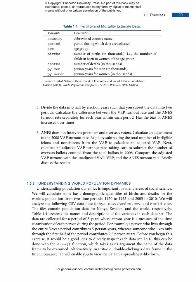
Table 1.4. Fertility and Mortality Estimate Data.
Variable Descriptioncountry abbreviated country nameperiod period during which data are collectedage age groupbirths number of births (in thousands), i.e., the number of
children born to women of the age groupdeaths number of deaths (in thousands)py.men person-years for men (in thousands)py.women person-years for women (in thousands)
Source: United Nations, Department of Economic and Social Affairs, PopulationDivision (2013).World Population Prospects: The 2012 Revision, DVD Edition.
5. Divide the data into half by election years such that you subset the data into twoperiods. Calculate the difference between the VEP turnout rate and the ANESturnout rate separately for each year within each period. Has the bias of ANESincreased over time?
6. ANES does not interview prisoners and overseas voters. Calculate an adjustmentto the 2008 VAP turnout rate. Begin by subtracting the total number of ineligiblefelons and noncitizens from the VAP to calculate an adjusted VAP. Next,calculate an adjusted VAP turnout rate, taking care to subtract the number ofoverseas ballots counted from the total ballots in 2008. Compare the adjustedVAP turnout with the unadjusted VAP, VEP, and the ANES turnout rate. Brieflydiscuss the results.
1.5.2 UNDERSTANDING WORLD POPULATION DYNAMICSUnderstanding population dynamics is important for many areas of social science.
We will calculate some basic demographic quantities of births and deaths for theworld’s population from two time periods: 1950 to 1955 and 2005 to 2010. We willanalyze the following CSV data files: Kenya.csv, Sweden.csv, and World.csv.The files contain population data for Kenya, Sweden, and the world, respectively.Table 1.4 presents the names and descriptions of the variables in each data set. Thedata are collected for a period of 5 years where person-year is a measure of the timecontribution of each person during the period. For example, a personwho lives throughthe entire 5-year period contributes 5 person-years, whereas someone who lives onlythrough the first half of the period contributes 2.5 person-years. Before you begin thisexercise, it would be a good idea to directly inspect each data set. In R, this can bedone with the View() function, which takes as its argument the name of the dataframe to be examined. Alternatively, in RStudio, double-clicking a data frame in theEnvironment tab will enable you to view the data in a spreadsheet-like form.
© Copyright, Princeton University Press. No part of this book may be distributed, posted, or reproduced in any form by digital or mechanical means without prior written permission of the publisher.
For general queries, contact [email protected]

January 5, 2017 Time: 12:08pm Chapter1.tex
30 Chapter 1: Introduction
1. We begin by computing crude birth rate (CBR) for a given period. The CBR isdefined as
CBR = number of births
number of person-years lived.
Compute the CBR for each period, separately for Kenya, Sweden, and the world.Start by computing the total person-years, recorded as a new variable within eachexisting data frame via the $ operator, by summing the person-years for men andwomen. Then, store the results as a vector of length 2 (CBRs for two periods) foreach region with appropriate labels. You may wish to create your own functionfor the purpose of efficient programming. Briefly describe patterns you observein the resulting CBRs.
2. The CBR is easy to understand but contains both men and women of all ages inthe denominator. We next calculate the total fertility rate (TFR). Unlike the CBR,the TFR adjusts for age compositions in the female population. To do this, weneed to first calculate the age-specific fertility rate (ASFR), which represents thefertility rate for women of the reproductive age range [15, 50). The ASFR for theage range [x, x+δ), where x is the starting age and δ is the width of the age range(measured in years), is defined as
ASFR[x, x+δ) = number of births to women of age [x, x + δ)number of person-years lived by women of age [x, x + δ)
.
Note that square brackets, [ and ], include the limit whereas parentheses, ( and ),exclude it. For example, [20, 25) represents the age range that is greater than orequal to 20 years old and less than 25 years old. In typical demographic data, theage range δ is set to 5 years. Compute the ASFR for Sweden and Kenya as well asthe entire world for each of the two periods. Store the resulting ASFRs separatelyfor each region. What does the pattern of these ASFRs say about reproductionamong women in Sweden and Kenya?
3. Using the ASFR, we can define the TFR as the average number of children thatwomen give birth to if they live through their entire reproductive age:
TFR = ASFR[15, 20) × 5 + ASFR[20, 25) × 5 + · · · + ASFR[45, 50) × 5.
We multiply each age-specific fertility rate by 5 because the age range is 5 years.Compute the TFR for Sweden and Kenya as well as the entire world for eachof the two periods. As in the previous question, continue to assume that thereproductive age range of women is [15, 50). Store the resulting two TFRs foreach country or the world as vectors of length 2. In general, how has the numberof women changed in the world from 1950 to 2000?What about the total numberof births in the world?
4. Next, we will examine another important demographic process: death. Computethe crude death rate (CDR), which is a concept analogous to the CBR, for each
© Copyright, Princeton University Press. No part of this book may be distributed, posted, or reproduced in any form by digital or mechanical means without prior written permission of the publisher.
For general queries, contact [email protected]
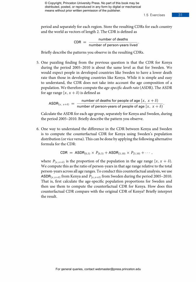
January 5, 2017 Time: 12:08pm Chapter1.tex
1.5 Exercises 31
period and separately for each region. Store the resulting CDRs for each countryand the world as vectors of length 2. The CDR is defined as
CDR = number of deaths
number of person-years lived.
Briefly describe the patterns you observe in the resulting CDRs.
5. One puzzling finding from the previous question is that the CDR for Kenyaduring the period 2005–2010 is about the same level as that for Sweden. Wewould expect people in developed countries like Sweden to have a lower deathrate than those in developing countries like Kenya. While it is simple and easyto understand, the CDR does not take into account the age composition of apopulation. We therefore compute the age-specific death rate (ASDR). The ASDRfor age range [x, x + δ) is defined as
ASDR[x, x+δ) = number of deaths for people of age [x, x + δ)number of person-years of people of age [x, x + δ)
.
Calculate the ASDR for each age group, separately for Kenya and Sweden, duringthe period 2005–2010. Briefly describe the pattern you observe.
6. One way to understand the difference in the CDR between Kenya and Swedenis to compute the counterfactual CDR for Kenya using Sweden’s populationdistribution (or vice versa). This can be done by applying the following alternativeformula for the CDR:
CDR = ASDR[0,5) × P[0,5) + ASDR[5,10) × P[5,10) + · · · ,
where P[x,x+δ) is the proportion of the population in the age range [x, x + δ).We compute this as the ratio of person-years in that age range relative to the totalperson-years across all age ranges. To conduct this counterfactual analysis, we useASDR[x,x+δ) from Kenya and P[x,x+δ) from Sweden during the period 2005–2010.That is, first calculate the age-specific population proportions for Sweden andthen use them to compute the counterfactual CDR for Kenya. How does thiscounterfactual CDR compare with the original CDR of Kenya? Briefly interpretthe result.
© Copyright, Princeton University Press. No part of this book may be distributed, posted, or reproduced in any form by digital or mechanical means without prior written permission of the publisher.
For general queries, contact [email protected]