quantitative storytelling in social convergence analysis€¦ · composite indicators are very...

QUANTITATIVE STORYTELLING IN SOCIAL CONVERGENCE ANALYSIS

Marta Kuc @kuc_marta,

Faculty of Management and Economics, Gdansk University of Technology Andrea Saltelli @AndreaSaltelli,

Centre for the Study of the Sciences and the Humanities, University of Bergen

Presentation plan

1. Introduction

2. The fortune of composite indicators

3. Quantitative story telling

4. Methodology

5. Research findings 1. National vs. regional

2. Different stakeholders

6. Conclusion

7. Further research

Introduction

Can composite indicator tell more than one story?

Convergence analysis

Experiment: Fixing the structure of CI while changing its scale,

Fixing its scale and changing the composition of its pillar

The fortune of composite indicators

Figure 1, Search on www.scopus.com using as search string: TITLE-ABS-KEY("composite indicator*") OR TITLE-ABS-KEY("composite index") OR T

ITLE-ABS-KEY("composite indices").

http://www.scopus.com/





The fortune of composite indicators

Composite indicators are very popular in analysis of:

Well-being

Communication technology development

Innovation

Health care system performance

Real estate market analysis

Countries/regions’ competitiveness

Quality of institution

Sustainable development

Standard of living

New wave of CI – spatial composite indicators

Pros of composite indicators

Can summarise complex, multi-dimensional realities with a view to supporting decision makers

Are easier to interpret than a battery of many separate indicators

Can assess progress of countries over time

Reduce the visible size of a set of indicators without dropping the underlying information base

Facilitate communication with general public

Enable users to compare complex dimensions effectively

Cons of composite indicators

May send misleading policy messages if poorly constructed or misinterpreted

May invite simplistic policy conclusions

May be misused – e.g. to support desired policy

The selection of indicators and weight could be the subject of political dispute

May lead to inappropriate policies if dimensions of performance that are difficult to measure are ignored

May fall short in the context of policy analysis and negotiation, where different options and different ‘end in sight’ are relevant

Two types of indices

According to Ravallion:

Those built on economic theory – direct monetary aggregates or based on shadow prices

‘mashup indices’ – HDI, MPI

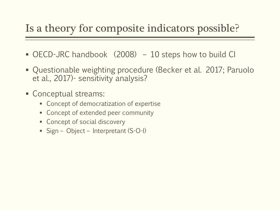
Is a theory for composite indicators possible?

OECD-JRC handbook (2008) – 10 steps how to build CI

Questionable weighting procedure (Becker et al. 2017; Paruolo et al., 2017)- sensitivity analysis?

Conceptual streams: Concept of democratization of expertise

Concept of extended peer community

Concept of social discovery

Sign – Object – Interpretant (S-O-I)

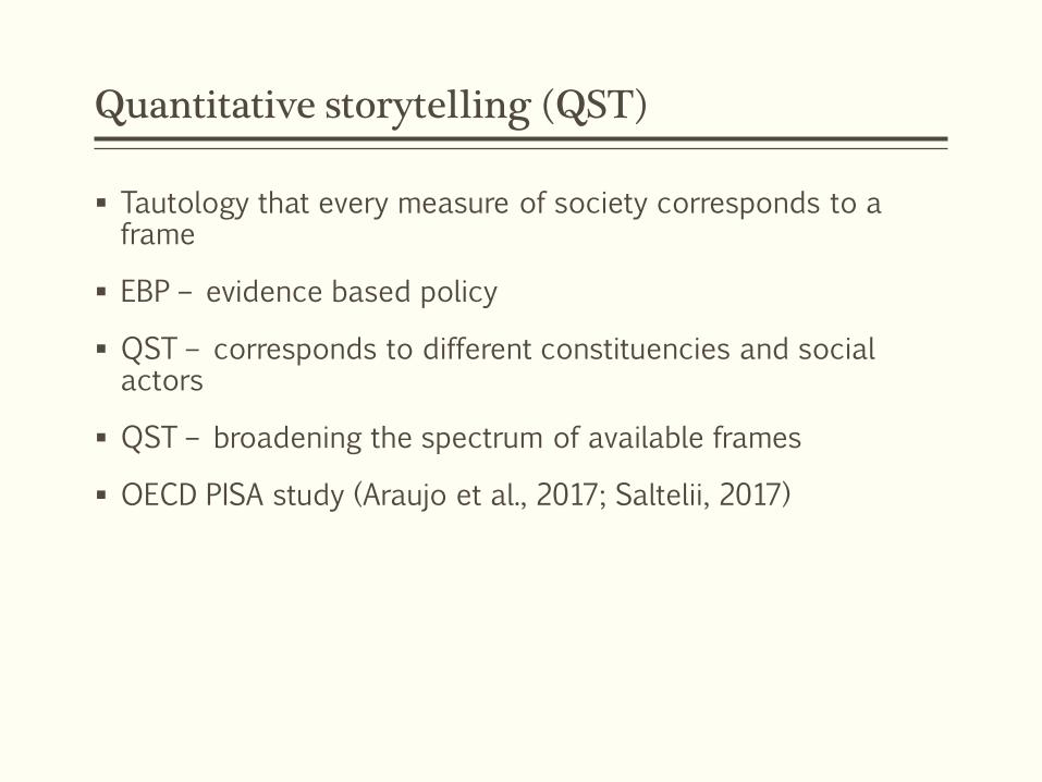
Quantitative storytelling (QST)

Tautology that every measure of society corresponds to a frame

EBP – evidence based policy

QST – corresponds to different constituencies and social actors

QST – broadening the spectrum of available frames

OECD PISA study (Araujo et al., 2017; Saltelii, 2017)

Methodology - CI

The classical approach to constructing composite indicators implies the assignment of variables to a given pillar (based on researchers’ own knowledge or experts opinion), then aggregation of variables within the pillar, and finally the aggregation into a holistic composite indicator. In our paper we decided to follow that the most popular approach.

Methodology - CI

Destimulants transformation:

Normalization formula:

ijt

s

ijtx

x1

2005,

'

max ij

ijt

ijtx

xx

Methodology - CI

Composite indicator

p

q

iqtit zp

CI1

1

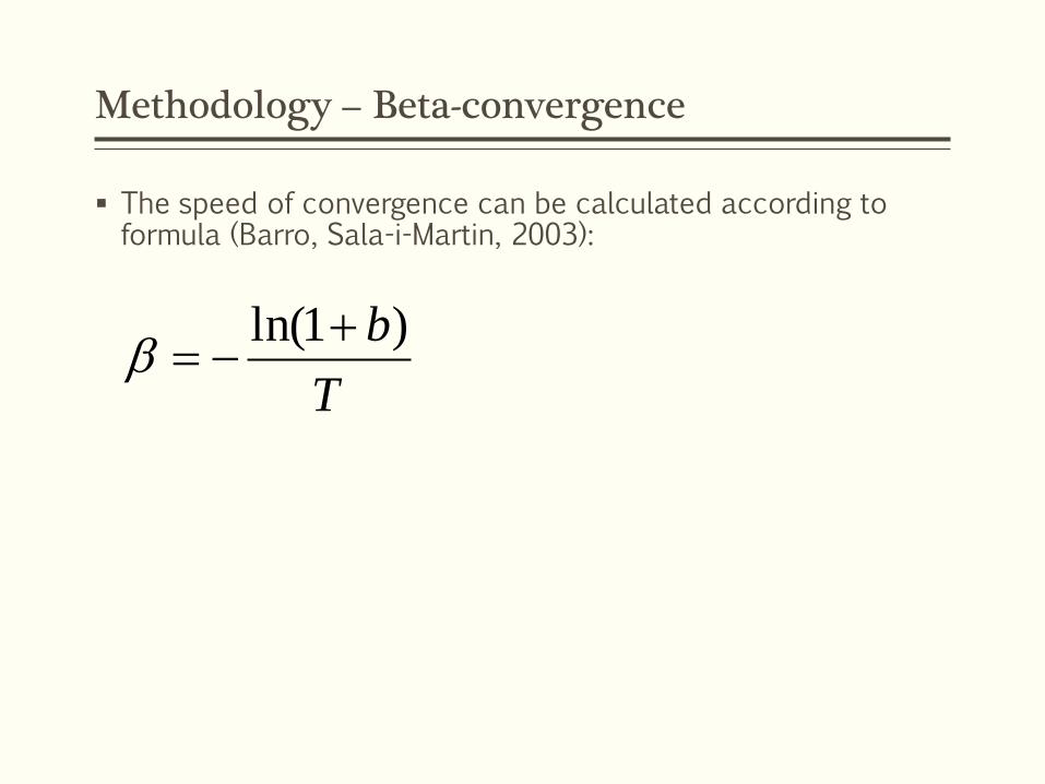
Methodology – Beta-convergence

Beta convergence is a process in which countries with lower performance are improving faster than those with higher one (Sala-i- Martin, 1996).

tii CIbag 0,log

0,

,log

1

i

Ti

iCI

CI

Tg

Methodology – Beta-convergence

The speed of convergence can be calculated according to formula (Barro, Sala-i-Martin, 2003):

T

b)1ln(

Methodology – Sigma-convergence

As it was mentioned before the occurrence of beta-convergence is a necessary condition for sigma-convergence, however based on the same equation we can investigate the existence of sigma-divergence (Friedman, 1992; Quah, 1993). To do so the following linear trend model was estimated:

tW tV 10

CI

L

lCICI

V

n

i

ii

W

1

2

Research findings – same composites at different scales

EU countries vs. EU NUTS-2 regions

Variables: Employment rate

Households income in PPS per capita

Long term unemployment

Participation rate in education and training

NEET – young people neither in employment nor in education and training

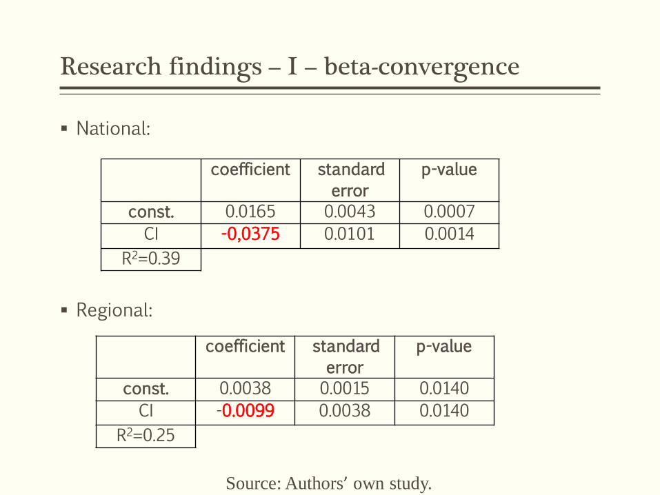
Research findings – I – beta-convergence

National:

Regional:

coefficient standard

error

p-value

const. 0.0165 0.0043 0.0007

CI -0,0375 0.0101 0.0014

R2=0.39

coefficient standard

error

p-value

const. 0.0038 0.0015 0.0140

CI -0.0099 0.0038 0.0140

R2=0.25

Source: Authors’ own study.

Research findings – I – speed of convergence

National:

Regional:

%35.0

%09.0

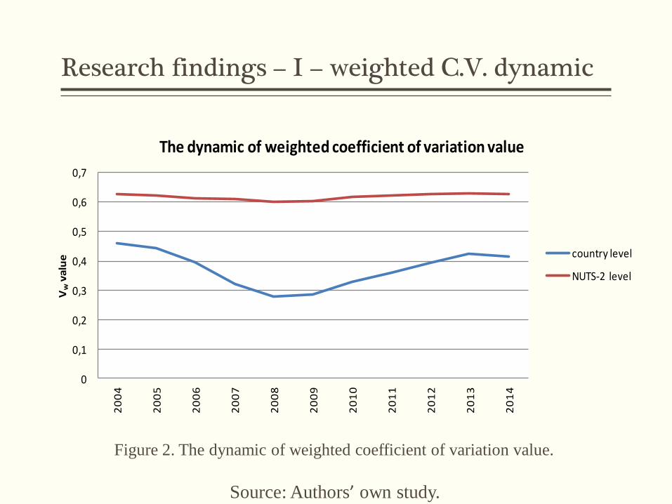
Research findings – I – weighted C.V. dynamic

0

0,1

0,2

0,3

0,4

0,5

0,6

0,7

20

04

20

05

20

06

20

07

20

08

20

09

20

10

20

11

20

12

20

13

20

14

Vw

va

lue

The dynamic of weighted coefficient of variation value

country level

NUTS-2 level

Figure 2. The dynamic of weighted coefficient of variation value.


Research findings – I – sigma convergence

0 1 R2

country level 0.3832 (0.000)

-0.0017 (0.7938)

0.0178

NUTS-2 level 0.6128 (0.000)

0.0009 (0.3695)

0.0918


Research findings – I – within countries disproportions

Convergence Divergence No evidence

1. Belgium 2. Germany 3. France 4. Hungary 5. Austria 6. Slovakia 7. Sweden

1. Denmark 2. Greece 3. Spain 4. Croatia 5. Italy 6. Portugal 7. Romania 8. Slovenia 9. Unitied Kingdom

1. Bulgaria 2. Czech Rep. 3. Ireland 4. Netherlands 5. Poland 6. Finland


Research findings – I – capital vs. other regions


Research findings – Same scale different pillars

Stakeholder 1 Stakeholder 2 Stakohlder 3 Stakholder 4

1. Opportunities and access to the labour market

2. Dynamic labour market and fair working condition

3. Public support/ Social protection and inclusion




4. Governance / Fairness




4. Functioning of health care




4. Governance/ Fairness

5. Functioning of health care

Research findings – II – Beta-convergence

Stakeholder no.1 coefficient standard error p-value

const. 0.0009 0.0020 0.6430

CI -0.0093 0.0072 0.2050

R2=0.2612


const. -0.0001 0.0018 0.9506

CI -0.0083 0.0064 0.2047

R2=0.28


const. 0.0066 0.0036 0.0813

CI 0.0022 0.0122 0.8572

R2=0.12


const. 0.0034 0.0028 0.2394

CI -0.0038 0.0093 0.6842

R2=0.25


Research findings – II – CI C.V. dynamic

0,1

0,125

0,15

0,175

0,2

0,225

0,25

0,275

2005 2006 2007 2008 2009 2010 2011 2012 2013 2014 2015 2016

Stakeholder 1 Stakeholder 2 Stakeholder 3 Stakeholder 4

Figure 3. The dynamic of coefficient of variation of CI value.


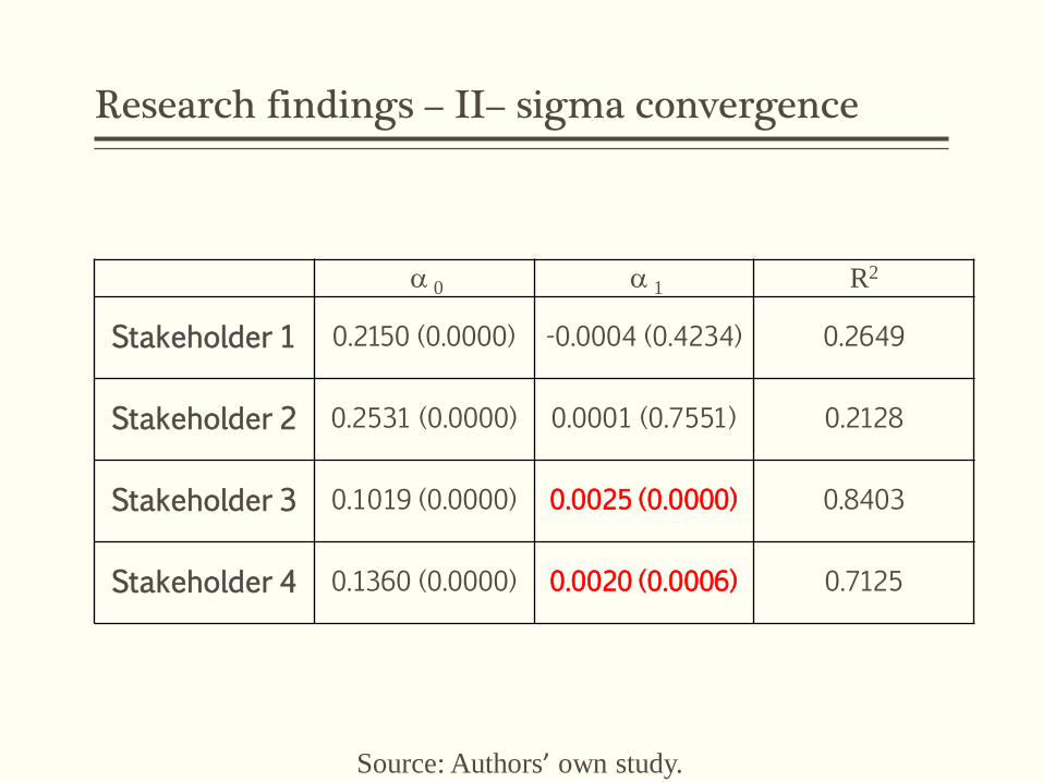
Research findings – II– sigma convergence

0 1 R2

Stakeholder 1 0.2150 (0.0000) -0.0004 (0.4234) 0.2649

Stakeholder 2 0.2531 (0.0000) 0.0001 (0.7551) 0.2128

Stakeholder 3 0.1019 (0.0000) 0.0025 (0.0000) 0.8403

Stakeholder 4 0.1360 (0.0000) 0.0020 (0.0006) 0.7125


Conclusions

Modification of philosophy of CI

Cohesion policy offers a convenient battleground to test this methodology

Is countries convergence more important than regional or within-country?

Should fairness be targeted by a cohesion policy?

Should health care be targeted by a cohesion policy?

Further research

Refining the analysis with more data

Rebalancing weights to their target importance using SA

Dynamic spatial panel model

THANK YOU

[email protected] [email protected]

mailto:[email protected]

quantitative storytelling in social convergence analysis€¦ · composite indicators are very...

Documents