quantitative structure-activity relationship: prediction
TRANSCRIPT

QUANTITATIVE STRUCTURE-ACTIVITY
RELATIONSHIP: PREDICTION OF
ANAEROBIC TRANSFORMATION
OF CHLOROACETANILIDE
HERBICIDES
By
ANGELA ROBYN KANA
Bachelor of Science
Oklahoma State University
Stillwater, Oklahoma
2005
Submitted to the Faculty of theGraduate College of the
Oklahoma State Universityin partial fulfillment ofthe requirements for
the degree ofMASTER OF SCIENCE
July, 2007

QUANTITATIVE STRUCTURE-ACTIVITY
RELATIONSHIP: PREDICTION OF
ANAEROBIC TRANSFORMATION
OF CHLOROACETANILIDE
HERBICIDES
Thesis Approved:
Dr. Gregory Wilber - Thesis Advisor
Dr. Dee Ann Sanders
Dr. Darrell Berlin
Dr. A. Gordon Emslie - Dean of the Graduate College
ii

Acknowledgments
I would like to express my genuine thanks to all the extraordinary individuals who
have contributed to the completion of this thesis through their illimitable and in-
valuable support. Of utmost importance is the work and influence of God on my
professors, friends and family shown by their perpetual encouraging advice and heart-
felt hugs. I am especially grateful to my thesis advisor, Dr. Gregory Wilber, for all
his patience, time, knowledge and faith during the course of this research project.
His relentless guidance, optimism, financial support and humor were driving forces
of this thesis and without these, this work would not be completed. Not only do I
thank Dr. Wilber for this work, but many thanks are due for his uncanny ability to
teach students and inspire numerous students, like myself, to leave the dark side of
the force of structural engineering and pursue a career in environmental engineering.
Additionally, I thank Dr. Wilber for nifty athletic team name recommendations such
as BOD5 and Sludge.
I would also like to extend many thanks to the other thesis committee mem-
bers and pseudo-committee member: Dr. Dee Ann Sanders, Dr. Darrell Berlin and
Dr. Nicholas Materer. To Dr. Sanders I owe my sincere appreciation for her emotional
support and understanding in my undergraduate and graduate education. With more
professors with her compassion for the environment, this world would definitely be a
better place with birds being heard worldwide and cookies putting smiles on many
faces. To Dr. Berlin I am beholden to for his insightful advisement and enthusiastic
iii
support. He is not only a distinguished professor of research but moreover, a teacher
countless students will always remember as grandpa Berlin for his endearing laugh-
ter in class and compassion to better our educational experiences. Lastly, I wish to
express my ineffable gratitude to Dr. Nicholas Materer for all his time and work and
valuable insight put forth into the research process. Most of all, I thank Dr. Materer
for his blunt (harsh but necessary) advice in completing the writing of this thesis.
Many thanks go to Tony Walker and Yanyan Qin for initiating this research project
through their hard work during their graduate college careers. Also, thanks to Justin
Clark for helping me with Latex and encouraging me to do well.
This work is dedicated to my friends and family members for their emotional
support over the last 7 years of my college life. Special thanks to my twin, Andrew,
for all his love and encouragement and unending faith in me. Also, special thanks
extended to my dear friends - Kevin Burns, Marty Goode, Mark Krzmarzick and
Kevin Sesock - for their comforting words and immovable confidence in me. More
than all others, I thank J.D. McElhaney for his study-buddy support for many sleep-
deprived and coffee-overdosed nights at IHOP.
In addition to those names mentioned above, I thank Doug Schrantz, Lizanne
Douglas, Daphne Rajenthiram, Zhazira Bausatova, Derek Henderson, Annette, Bu-
lard family and Paula Hart for adding unforgettable laughter, smiles, hugs, prayers
and thrilling experiences to my life.
I would like to thank the all those in funding my graduate education through
scholarships, assistantships or employment opportunities: Dr. Wilber, Ponca City
Community Christian Church, Pawnee United Methodist Church, College of Engi-
neering, Architecture and Technology Student Services, Society of American Military
Engineers, Kyoto Japanese Restaurant and Marianne and George Bulard.
iv

Contents
1 Introduction 1
1.1 Motivation . . . . . . . . . . . . . . . . . . . . . . . . . . . . . . . . . 2
1.2 Contribution . . . . . . . . . . . . . . . . . . . . . . . . . . . . . . . . 3
1.3 Thesis Outline . . . . . . . . . . . . . . . . . . . . . . . . . . . . . . . 5
2 Literature Review 6
2.1 Introduction . . . . . . . . . . . . . . . . . . . . . . . . . . . . . . . . 6
2.2 Pesticide Contaminated Groundwater . . . . . . . . . . . . . . . . . . 7
2.3 Pesticide Contaminated Groundwater Sources . . . . . . . . . . . . . 8
2.4 Transport of Xenobiotic Chemicals . . . . . . . . . . . . . . . . . . . 9
2.4.1 Dissolution and Solubility . . . . . . . . . . . . . . . . . . . . 9
2.4.2 Volatilization . . . . . . . . . . . . . . . . . . . . . . . . . . . 10
2.4.3 Sorption . . . . . . . . . . . . . . . . . . . . . . . . . . . . . . 11
2.4.4 Advection and Hydrodynamic Dispersion . . . . . . . . . . . . 11
2.5 Transformation of Xenobiotic Chemicals . . . . . . . . . . . . . . . . 12
2.5.1 Biotransformation . . . . . . . . . . . . . . . . . . . . . . . . . 12
2.5.2 Chemical Transformation . . . . . . . . . . . . . . . . . . . . . 13
2.6 Anaerobic Transformation: Abiotic and Biotic Reactions of Halogenated
Compounds . . . . . . . . . . . . . . . . . . . . . . . . . . . . . . . . 14
2.6.1 Impact of Bisulfide . . . . . . . . . . . . . . . . . . . . . . . . 15
v

2.6.2 Impact of Nitrate Reduction . . . . . . . . . . . . . . . . . . . 16
2.7 Pesticide Analysis and Transformation
Kinetics . . . . . . . . . . . . . . . . . . . . . . . . . . . . . . . . . . 18
2.7.1 Experimental Systems with Bisulfide . . . . . . . . . . . . . . 19
2.7.2 Experimental Systems with Denitrifying Bacterial
Culture . . . . . . . . . . . . . . . . . . . . . . . . . . . . . . 21
2.7.3 Bisulfide and Nitrate-reducing Rate of Transformation Constants 23
2.8 Quantitative Structure-Activity Relationships . . . . . . . . . . . . . 24
2.8.1 Underlying Principles of QSARs . . . . . . . . . . . . . . . . 24
2.8.2 QSAR Model . . . . . . . . . . . . . . . . . . . . . . . . . . . 25
2.8.3 QSAR Model Validation . . . . . . . . . . . . . . . . . . . . . 25
2.8.4 QSAR Descriptors . . . . . . . . . . . . . . . . . . . . . . . . 26
2.8.5 Octanol-water Partition Coefficient Descriptors . . . . . . . . 28
2.8.6 QSAR and Chloroacetanilide Degradation . . . . . . . . . . . 28
2.9 QSAR and Chloroacetanilide Transformation . . . . . . . . . . . . . . 28
2.9.1 Chloroacetanilides . . . . . . . . . . . . . . . . . . . . . . . . 29
2.9.2 Acetochlor . . . . . . . . . . . . . . . . . . . . . . . . . . . . . 36
2.9.3 Butachlor . . . . . . . . . . . . . . . . . . . . . . . . . . . . . 37
2.9.4 Metolachlor . . . . . . . . . . . . . . . . . . . . . . . . . . . . 38
2.9.5 Propachlor . . . . . . . . . . . . . . . . . . . . . . . . . . . . . 39
2.10 Literature Values of Chloroacetanilide
Properties . . . . . . . . . . . . . . . . . . . . . . . . . . . . . . . . . 39
2.11 Summary . . . . . . . . . . . . . . . . . . . . . . . . . . . . . . . . . 40
3 Methods and Materials 41
3.1 Introduction . . . . . . . . . . . . . . . . . . . . . . . . . . . . . . . . 41
3.2 CambridgeSoftr Software: ChemOffice 2006r
Experimental Tools . . . . . . . . . . . . . . . . . . . . . . . . . . . . 42
vi

3.2.1 ChemDraw Pro 10.0 R© . . . . . . . . . . . . . . . . . . . . . . 42
3.2.2 Chem3D Pro 10.0 R© . . . . . . . . . . . . . . . . . . . . . . . 42
3.3 Gaussian 03r Software Tool . . . . . . . . . . . . . . . . . . . . . . . 44
3.4 Literature Comparison of Software Computed Properties . . . . . . . 44
3.5 Microsoft Excelr Statistical Analysis . . . . . . . . . . . . . . . . . . 44
4 Results and Discussion 47
4.1 Introduction . . . . . . . . . . . . . . . . . . . . . . . . . . . . . . . . 47
4.2 Bisulfide and Nitrate Reduction Degradation Analyses . . . . . . . . 47
4.3 Chem3D Pro 10.0r Computation Results . . . . . . . . . . . . . . . . 48
4.3.1 Molecular Mechanics . . . . . . . . . . . . . . . . . . . . . . . 48
4.3.2 Property Computations . . . . . . . . . . . . . . . . . . . . . 50
4.4 Statistical Analysis Discussion . . . . . . . . . . . . . . . . . . . . . . 52
4.4.1 Thermodynamic Property-Kinetics Correlations . . . . . . . . 53
4.4.2 Steric-, Electronic- and Atomic-Kinetics
Correlations . . . . . . . . . . . . . . . . . . . . . . . . . . . . 56
4.5 Summary of QSAR Descriptor Statistical
Analysis . . . . . . . . . . . . . . . . . . . . . . . . . . . . . . . . . . 61
5 Conclusions and Future Work 64
5.1 Conclusions . . . . . . . . . . . . . . . . . . . . . . . . . . . . . . . . 64
5.2 Recommendations for Further Research . . . . . . . . . . . . . . . . . 66
A Rate Constants, Descriptor Values, Correlation Plots 81
A.1 Bisulfide and Nitrate-reducing Rate Constants . . . . . . . . . . . . . 81
A.2 Descriptor Values . . . . . . . . . . . . . . . . . . . . . . . . . . . . . 82
A.3 Correlation Values between Descriptors and Rate Constants . . . . . 83
A.4 Correlation Plots . . . . . . . . . . . . . . . . . . . . . . . . . . . . . 84
A.5 Molecular Mechanics Figures . . . . . . . . . . . . . . . . . . . . . . . 129
vii

List of Figures
2.1 Alachlor structure and properties. . . . . . . . . . . . . . . . . . . . . 29
2.2 Acetochlor structure and properties. . . . . . . . . . . . . . . . . . . . 30
2.3 Butachlor structure and properties. . . . . . . . . . . . . . . . . . . . 31
2.4 Metolachlor structure and properties. . . . . . . . . . . . . . . . . . . 32
2.5 Propachlor structure and properties. . . . . . . . . . . . . . . . . . . 33
4.1 Butachlor before energy minimization. . . . . . . . . . . . . . . . . . 49
4.2 Butachlor after energy minimization. . . . . . . . . . . . . . . . . . . 50
4.3 kHS− and Connolly excluded solvent volume correlation plot. . . . . . 57
4.4 kHS− and Connolly molecular area correlation plot. . . . . . . . . . . 58
4.5 kHS− and molecular weight correlation plot. . . . . . . . . . . . . . . 59
A.1 kHS− and ln(Kow) correlation plot. . . . . . . . . . . . . . . . . . . . 85
A.2 ln(kHS−) and ln(Kow) correlation plot. . . . . . . . . . . . . . . . . . 86
A.3 kbio and ln(Kow) correlation plot. . . . . . . . . . . . . . . . . . . . . 87
A.4 ln(kbio) and ln(Kow) correlation plot. . . . . . . . . . . . . . . . . . . 88
A.5 kHS− and KH correlation plot. . . . . . . . . . . . . . . . . . . . . . . 89
A.6 ln(kHS−) and KH correlation plot. . . . . . . . . . . . . . . . . . . . . 90
A.7 kbio and KH correlation plot. . . . . . . . . . . . . . . . . . . . . . . . 91
A.8 ln(kbio) and KH correlation plot. . . . . . . . . . . . . . . . . . . . . . 92
A.9 kHS− and solubility correlation plot. . . . . . . . . . . . . . . . . . . . 93
viii

A.10 ln(kHS−) and solubility correlation plot. . . . . . . . . . . . . . . . . . 94
A.11 kbio and solubility correlation plot. . . . . . . . . . . . . . . . . . . . . 95
A.12 ln(kbio) and solubility correlation plot. . . . . . . . . . . . . . . . . . . 96
A.13 kHS− and molar refractivity correlation plot. . . . . . . . . . . . . . . 97
A.14 ln(kHS−) and solubility correlation plot. . . . . . . . . . . . . . . . . . 98
A.15 kbio and molar refractivity correlation plot. . . . . . . . . . . . . . . . 99
A.16 ln(kbio) and molar refractivity correlation plot. . . . . . . . . . . . . . 100
A.17 kHS− and molecular weight correlation plot. . . . . . . . . . . . . . . 101
A.18 ln(kHS−) and solubility correlation plot. . . . . . . . . . . . . . . . . . 102
A.19 kbio and molecular weight correlation plot. . . . . . . . . . . . . . . . 103
A.20 ln(kbio) and molecular weight correlation plot. . . . . . . . . . . . . . 104
A.21 kHS− and Connolly molecular area correlation plot. . . . . . . . . . . 105
A.22 ln(kHS−) and Connolly molecular area correlation plot. . . . . . . . . 106
A.23 kbio and Connolly molecular area correlation plot. . . . . . . . . . . . 107
A.24 ln(kbio) and Connolly molecular area correlation plot. . . . . . . . . . 108
A.25 kHS− and Connolly excluded solvent volume correlation plot. . . . . . 109
A.26 ln(kHS−) and Connolly excluded solvent volume correlation plot. . . . 110
A.27 kbio and Connolly excluded solvent volume correlation plot. . . . . . . 111
A.28 ln(kbio) and Connolly excluded solvent volume correlation plot. . . . . 112
A.29 kHS− and dipole moment correlation plot. . . . . . . . . . . . . . . . 113
A.30 ln(kHS−) and dipole moment correlation plot. . . . . . . . . . . . . . 114
A.31 kbio and dipole moment correlation plot. . . . . . . . . . . . . . . . . 115
A.32 ln(kbio) and dipole moment correlation plot. . . . . . . . . . . . . . . 116
A.33 kHS− and C-Cl bond length correlation plot. . . . . . . . . . . . . . . 117
A.34 ln(kHS−) and C-Cl bond length correlation plot. . . . . . . . . . . . . 118
A.35 kbio and C-Cl bond length correlation plot. . . . . . . . . . . . . . . . 119
A.36 ln(kbio) and C-Cl bond length correlation plot. . . . . . . . . . . . . . 120
ix

A.37 kHS− and C-Cl bond energy correlation plot. . . . . . . . . . . . . . . 121
A.38 ln(kHS−) and C-Cl bond energy correlation plot. . . . . . . . . . . . . 122
A.39 kbio and C-Cl bond energy correlation plot. . . . . . . . . . . . . . . . 123
A.40 ln(kbio) and C-Cl bond energy correlation plot. . . . . . . . . . . . . . 124
A.41 kHS− and C=O carbon charge correlation plot. . . . . . . . . . . . . . 125
A.42 ln(kHS−) and C=O carbon charge correlation plot. . . . . . . . . . . . 126
A.43 kbio and C=O carbon charge correlation plot. . . . . . . . . . . . . . . 127
A.44 ln(kbio) and C=O carbon charge correlation plot. . . . . . . . . . . . . 128
A.45 Alachlor before energy minimization. . . . . . . . . . . . . . . . . . . 129
A.46 Alachlor after energy minimization. . . . . . . . . . . . . . . . . . . . 129
A.47 Acetochlor before energy minimization. . . . . . . . . . . . . . . . . . 130
A.48 Acetochlor after energy minimization. . . . . . . . . . . . . . . . . . . 130
A.49 Butachlor before energy minimization. . . . . . . . . . . . . . . . . . 131
A.50 Butachlor after energy minimization. . . . . . . . . . . . . . . . . . . 131
A.51 Metolachlor before energy minimization. . . . . . . . . . . . . . . . . 132
A.52 Metolachlor after energy minimization. . . . . . . . . . . . . . . . . . 132
A.53 Propachlor before energy minimization. . . . . . . . . . . . . . . . . . 133
A.54 Propachlor after energy minimization. . . . . . . . . . . . . . . . . . . 133
x

List of Tables
2.1 Bisulfide and biological rate reaction constants for chloroacetanilide
herbicides. . . . . . . . . . . . . . . . . . . . . . . . . . . . . . . . . . 23
4.1 Bisulfide and biological rate reaction constants for chloroacetanilide
herbicides. . . . . . . . . . . . . . . . . . . . . . . . . . . . . . . . . . 48
4.2 Percent difference between literature value and Chem3DPro 10.0 R© com-
putations for Kow. . . . . . . . . . . . . . . . . . . . . . . . . . . . . . 51
4.3 Thermodynamic properties of chloroacetanilide herbicides. . . . . . . 51
4.4 Chem3D Pro 10.0 R© steric and atomic properties of chloroacetanilide her-
bicides. . . . . . . . . . . . . . . . . . . . . . . . . . . . . . . . . . . . 51
4.5 Gaussian 03 R© electronic and steric properties of chloroacetanilide herbicides. 52
4.6 Correlations values between thermodynamic properties and rate con-
stants. . . . . . . . . . . . . . . . . . . . . . . . . . . . . . . . . . . . 52
4.7 Correlations values between atomic, electronic, and steric descriptors
and rate constants. . . . . . . . . . . . . . . . . . . . . . . . . . . . . 52
A.1 Bisulfide and biological rate reaction constants for chloroacetanilide
herbicides . . . . . . . . . . . . . . . . . . . . . . . . . . . . . . . . . 81
A.2 Descriptor Values . . . . . . . . . . . . . . . . . . . . . . . . . . . . . 82
A.3 Descriptor Values . . . . . . . . . . . . . . . . . . . . . . . . . . . . . 82
xi

A.4 Correlations values between thermodynamic properties and rate con-
stants . . . . . . . . . . . . . . . . . . . . . . . . . . . . . . . . . . . 83
A.5 Correlations values between atomic, electronic and steric descriptors
and rate constants . . . . . . . . . . . . . . . . . . . . . . . . . . . . 83
xii

Nomenclature and List of Symbols
C=O Carbonyl-carbon
CESV Connolly excluded solvent volume
CMA Connolly molecular area
KH Henry’s Constant
Kow Octanol-water partition coefficient
MR Molar Refractivity
MW Molecular weight
xiii

Chapter 1
Introduction
For thousands of years, humans have been in search of undiscovered areas for further
plant and animal development to support the booming population growth. In the
process of exploration, nature’s biological entities warranted the need for mitigating
the impedimental behavior of same plantae, fungi and animalia on the enrichment of
the earth’s resources. Particularly, weeds, plants and grasses erect barriers for optimal
production and utilization of primary croplands. To combat these hindrances, one
course humans have delved into is the design, manufacturing and implementation of
pesticides. Though these chemical advances help alleviate the arduous labor in crop
cultivation, initially scientists and engineers unknowingly set in place the beginning
of harmful environmental and public health obstacles.
The dominant backlash of uncontrolled applications of pesticides on croplands,
including those in the chloroacetanilide herbicide family (alachlor, acetochlor, propa-
chlor, butachlor and metolachlor), is the contamination of groundwater. Moreover,
these pollutants pose potential adverse animal and human health effects by way of
contaminated groundwater consumption. Approximately 23 million people in the
United States use untreated groundwater as their main source of drinking water while
the remainder of drinking water is treated with expensive technology or inadequate
1

treatment methods for the removal of pesticides [1]. Hence, research has turned
to understanding the pesticides’ fate and modifications in chemical structure (i.e.
transformation) when undergoing water treatment and while moving through the
subsurface.
1.1 Motivation
The fate and transport of the chlorinated acetanilide pesticides is chiefly governed by
the type of transport medium (hydrogeology) where they are acted upon by physi-
cal, chemical and biological processes. Although some research has been performed
on the transformations occurring in surface waters and in subsurface layers under
methanogenic and sulfate-reducing conditions, there are only limited investigations
into quantifying the chemical and biological fate of these pesticides under other anaer-
obic transformations such as those with bisulfide and nitrate-reducing cultures. Pre-
vious research for example, has indicated that abiotic reactions occur between these
herbicides and bisulfide, possibly leading to dechlorination.
As previously stated, only limited research has been performed correlating the
chemical and biological degradation rate of chloroacetanilides to the alterations in
their chemical structures under anaerobic conditions in the presence of denitrifying
bacteria or bisulfide. However, the science of quantitative structure-activity relation-
ships (QSARs) can be used as a tool to not only correlate transformation rates to
compounds’ structures or properties but to predict transformation rates of other sim-
ilar compounds. Specifically, QSAR is a mathematical model used to relate known
activity of a congeneric series of compounds to their structure or properties to predict
other compounds’ unknown activity. QSARs have not been extensively investigated
for chloroacetanilide herbicides participating in abiotic and biotic reactions under
anaerobic conditions, though there is a considerable amount of toxicological QSAR
2

research.
Initially, QSARs were developed to predict the activity and properties of pharma-
ceuticals and pesticides, principally for conception and design purposes [2]. However,
as the need for cost-effective bioremediation techniques increased due to escalations in
environmental contamination, the original objective of QSARs expanded to encom-
pass the prediction of organic chemical properties and activities such as solubility,
Henry’s constant, and bioconcentration. Additionally, this technique can provide
insight into the causation and mechanism of physical, biological and chemical trans-
formations of contaminants. From such analyses can evolve effective bioremediation
technology and ultimately enhance the quality of the environment and public health.
Resources aiding the effort of establishing QSARs include chemical and biochemi-
cal software programs. For this thesis work, ChemDraw and Chem3D Pro 10.0 R© and
Gaussian 03 R© were used to measure structural characteristics and properties for chloroacet-
anilides. ChemDraw 10.0 R© allows the user to build any compound in two dimensions. From
this program, constructed compounds can be imported into Chem3D Pro 10.0R© where the
compounds are drawn in three dimensions and property/structural characteristics can be
calculated. Gaussian 03 R© is a similar program to Chem3D Pro 10.0R© , and comparisons of
properties computed in Chem3D Pro 10.0R© and Gaussian 03 R© can be made. These pro-
grams allow for timely property/structural calculations for compounds that otherwise would
require inexpedient experiments to determine the unavailable data of these compounds. The
use of such programs brings scientists and engineers closer to developing full-scale QSARs
and to understanding the remediation technology needed for the betterment of the environ-
ment.
1.2 Contribution
Chloroacetanilide herbicides demonstrate desirable pre- and post-emergence regulation of
weeds and grasses in an assortment of corn, cotton and soybean crops [3]. Additionally,
3

over the last two decades, more than 50 million kg of these herbicides have been used
annually in the United States for a variety of crops including soybeans, peanuts, corn,
wheat, broadleaf weeds, [4]. More importantly, studies have detected chloroacetanilides
and their metabolites in groundwater and surface waters ([5], [6]). Their presence in these
water sources raises concern since according to United States Environmental Protection
Agency, alachlor, acetochlor, metolachlor, and propachlor are considered to be carcinogenic
([7], [8], [9], [10]).
Because of their ubiquitous presence in groundwater, persistence and potential adverse
effects, five commonly used chloroacetanilide herbicides - alachlor, acetochlor, propachlor,
butachlor and metolachlor - were chosen for a research project to further investigate their en-
vironmental fates under anaerobic conditions through use of quantitative structure-activity
relationships. Among the main objectives of this research were the following:
1. To estimate solubility (S), Henry’s constant (KH), and octanol-water partition coef-
ficient (Kow) of selected herbicides - alachlor, acetochlor, propachlor, butachlor and
metolachlor - using ChemDraw Pro 10.0 R© and Chem3D Pro 10.0 R©,
2. To correlate the kinetic data of abiotic reactions between bisulfide and chloroacet-
anilide herbicides to their computed chemical structural and properties using Chem3D
Pro 10.0 R© and Gaussian 03 R©, and
3. To correlate the kinetic data of biotic reactions in nitrate-reducing cultures and
chloroacetanilide herbicides to their computed chemical structural descriptors and
properties using Chem3D Pro 10.0 R© and Gaussian 03 R©.
The overall goal of this thesis was to perform preliminary analyses that can be used in
a full-scale QSAR investigation for quantifying the abiotic and biotic degradation rates
chloroacetanilide herbicides under anaerobic conditions. Furthermore, these results can be
used as an initial reference point for similar research efforts on other pesticides.
4

1.3 Thesis Outline
Contained hereafter, Chapter 2 includes a discussion on the current literature. In particular,
this chapter prefaces the work performed by Walker [11] and Qin [12] regarding the trans-
formation and degradation kinetics of chloroacetanilides in nitrate-reducing and bisulfide
environments, respectively, which provide the original data used in this analysis. Chap-
ter 3 describes the methodology, materials and modeling tools adopted in these analyses.
The results and discussion of the research are presented in Chapter 4. Chapter 5 includes
the conclusions made from this work and recommendations for further research. Lastly,
Appendix A contains all collected data and constructed plots used in this work.
5

Chapter 2
Literature Review
2.1 Introduction
Over the past 20 years, a substantial amount of research has been performed in order
to gain a better understanding about the transformations of xenobiotic pesticides under
various conditions in groundwater and surface water. This research comprises a diverse
group of investigations from a multitude of scientific and engineering disciplines. Thus,
research analyses have entailed the following non-exhaustive list: water contamination sur-
veys (sources and prevalence), bioremediation investigations (treatment and removal), and
fate and transport studies (lab and in-situ).
This review of the literature will briefly summarize the significance of several research
accomplishments related to the QSAR work characterized in this thesis. Firstly, this re-
view discusses the persistence of pesticides in groundwater and their non-point and point
sources. Consecutively, a brief description of the health and environmental implications
of groundwater contamination will be presented, followed by a thorough delineation of the
research performed over the transformations of pesticides including descriptions of earlier
work performed by Qin [12] and Walker [11] that provide the original data for this thesis
research. Subsequent reviews include details of the selected chloroacetanilide herbicides
for this thesis research: alachlor, acetochlor, propachlor, butachlor and metolachlor. Fur-
6

thermore, this review describes the quantitative-structure activity relationship techniques
and the relation to degradation of chloroacetanilides. Finally, this section concludes with a
summary of this work’s literature assessment.
2.2 Pesticide Contaminated Groundwater
As previously stated, the blanketed applications of pesticides pose a potential threat to the
environment and public health as supported by various studies that have detailed numer-
ous cases of groundwater contamination by these chemicals. In 2000, the United States
utilized pesticides on over 900,000 farms and in 70 million homes of which the majority of
pesticides were herbicides [13]. This use resulted in the urban residences of northern United
States treating their lawns at an equivalent rate to that of farmers in the food production
industry. Consequently, the phenomenal use and persistence of pesticides in the northern
United States have led to approximately 75% of municipal wells and 70% of private wells
containing pesticides and their metabolites [14]. On a national basis, out of approximately
1500 domestic and public supply well samples taken throughout the U.S. between 1992 and
1996, about 40% were contaminated with pesticides [15]. According to the United States
Geological Survey, more than 50% of the wells tested contained pesticides in the water in
areas of agricultural and urban groundwater and more than 50% of the agricultural areas
contained herbicides between 1991 and 1997 [16].
Some of the most widely used chloroacetanilide herbicides in the United States include
alachlor, acetochlor, propachlor, butachlor and metolachlor [17]. In 1996, 1.15, 1.67, and
0.647 million pounds of alachlor, metolachlor and acetochlor were applied to corn crops in
Wisconsin, respectively. In the vicinity of these cropland areas, 70% of private wells con-
tained concentrations of an alachlor metabolite between 1.1 and 27 µg/L , and 7% contained
the parent compound alachlor [14]. In the southern United States during the early nineties,
over 50 and 15 tons of metolachlor and alachlor, respectively, were transported into the
Gulf of Mexico, via surface waters, completely contaminating the Mississippi River navi-
gable reach. Chloroacetanilides are also the dominant herbicides used for the corn crops
7

in Iowa accounting for 38% of herbicides used in this state. Thus, surveys have shown
that 75% of municipal wells were contaminated with metolachlor, alachlor, and acetochlor
metabolites with a median value of summed concentrations of 1.2 µg/L . Additionally, in
surface waters, the parent compounds had a median value of 6.4 µg/L [18]. Another study
in Iowa measured up to 16 µg/L of alachlor in groundwater [19]. There are many other stud-
ies that have shown groundwater contamination by chloroacetanilides and correspondingly
instigated various risk assessment studies.
According to the Environmental Protection Agency [20], these herbicides can promote
unsafe conditions for the ecological environment and human health. For example, acet-
ochlor, butachlor, and alachlor can result in tumors in the nasal olfactory epithelium and
thyroid. Though the EPA has concluded that metolachlor and propachlor do not cause such
tumors, the National Resource Defense Council (NRDC), World Wildlife Fund (WWF),
Consumers Union (CU), and Institute for Environment and Agriculture (IEA) have pre-
sented evidence that both chloroacetanilides display similar mechanisms. Therefore, all five
chloroacetanilides can induce oncogenic effects.
Currently, the EPA has set the drinking water Maximum Contaminant Level (MCL) for
alachlor at 2 µg/L or 2 ppb [21]. Acetochlor, butachlor, propachlor, and metolachlor await
further investigation to establish their MCLs but presently have unregulated monitoring
programs in place.
As evidenced by the information presented, chloroacetanilides currently pose potential
hazards to the environment and human health especially due to their unpredictable fre-
quency of contamination in groundwater and surface waters. Hence, an intermediate step
to elucidate the fate and transport of these chemicals begins with the understanding of their
sources.
2.3 Pesticide Contaminated Groundwater Sources
Herbicide contamination of groundwater stems from point-source or non-point-source pollu-
tion. Point-sources primarily encompass the facilities categorized in the commercial industry
8

and sometimes include those on a smaller scale such as accidental spills, back siphoning,
and storage leaking with on-farm usage. Non-point sources embody a much larger area,
predominantly where broadcast applications are made to crops or soil [19]. Historically, the
handling and use of herbicides were not monitored cautiously, resulting in multiple non-point
sources to be labeled point sources. The lack of discernment between the types of sources
inhibits the ability to curtail future problems with herbicide contamination. Though dis-
tinguishing between point sources and non-point-sources may be ambiguous at times, both
forms of release into the environment can conclusively initiate the transport of pollutants
into the topsoil, subsurfaces and groundwater.
Upon application, the fate and transport of herbicides are mostly dependent upon
their sorption and persistence. These processes occur along side other phenomena such as
volatilization, advection, chemical decomposition, biological degradation, photolysis, and
groundwater interactions [22]. In order to research methods to remediate herbicide-con-
taminated soils and groundwater, the exploitation of these fate processes by scientists and
engineers is essential.
2.4 Transport of Xenobiotic Chemicals
As previously mentioned, xenobiotic chemicals can enter the ground in various ways. In
doing so, they can enter the environment as a pure compound or as a solute, where they can
infiltrate through the topsoil, subsurfaces, and ultimately the groundwater. This behavior
is dictated by several processes such as solubilization, volatilization, sorption, advection,
and chemical/biological transformation. The following sections include brief descriptions of
each process.
2.4.1 Dissolution and Solubility
Upon contact with subsurface waters, xenobiotic compounds can be fully or partially dis-
solved into the water. The extent of dissolution is dependent upon the compound’s aqueous
solubility (i.e. hydrophilicity) - the amount of solute that dissolves in a known amount of
9

water at a specific temperature. For example, if a substance has a low solubility (i.e. is
highly hydrophobic), that chemical can be a separate liquid or solid, relative to the solvent,
or remain as a gas. Hence, the fate and transport of the substance will be primarily governed
by its relative density with respect to water and its volatilization potential and its tendency
to convert into a gas. In contrast, a compound with a high solubility is largely regulated by
its polarity and molecular size. Other factors affecting solubility include, but not limited
to, are nature/number/location of functional groups, pH, co-solutes, and temperature [2].
For pesticides, those with solubility greater than 30 mg/L in groundwater are considered
potentially unsafe. Characteristically en masse, chloroacetanilides have solubility greater
than 30 mg/L [23]. Alachlor, acetochlor, butachlor, and metolachlor have solubility values of
240, 223, 530, and 580 mg/L respectively [3]. Correspondingly, high solubility increases the
ability of the pollutant to move within the site or off-site via runoff or leaching. Furthermore,
dissolution in natural organic matter is the main activity underlying the process of sorption.
Therefore, an understanding of solubility assists in the comprehension and exploitation of
sorption properties of xenobiotic chemicals.
2.4.2 Volatilization
Corresponding to dissolution in understanding the fate and removal of organic contaminants
is the process of volatilization. Along with solubility, this concept is also described through
Henry’s constant, KH , which can be “thought of as a partition coefficient between water and
the atmosphere” [2]. This constant controls the accumulation tendency at equilibrium. In
particular, at a low KH , contaminants tend to accumulate in the aqueous phase in contrast
to those with a high KH partitioning more into the gaseous phase [24]. Upon establishing the
dominant phase of the contaminant, its fate thereafter depends on other chemical properties.
Henry’s constant has a strong dependency on temperature such that at a lower temperature,
compounds have lower volatility. This property is important in considering the widespread
application of herbicides and their exposure to humans. Hence, an understanding of this
phenomenon is needed for the remediation of herbicide contaminants to protect human
health.
10

2.4.3 Sorption
Another pertinent process contributing to the fate and transport and biological activity of
xenobiotic substances in the soil environment is sorption [25]. Sorption refers to absorption
and adsorption - the incorporation or uptake of an element by a cell or organism and physical
adhesion onto the surface of another liquid or solid [26]. In conjunction with sorption is
the process of desorption - the removal of substance from the surface of another. Sorption
is measured by the soil adsorption coefficient (Koc), particularly, the higher the Koc, the
stronger its adsorption to soil organic matter and the lesser its capability to leach into
the groundwater. These phenomena can be rate-limiting factors affecting biodegradability,
bioavailability, subsurface transport, and bioremediation. Specifically, they influence the
amount of contaminant in the aqueous phase, on aquifer solids, and retardation/attenuation
in groundwater ([25], [27]).
The sorption potential of a substance is dependent on the chemical/physical properties
of the sorbate and sorbent. Such properties can include hydrophobicity, molecular size, and
fraction of organic matter in soils and aquifer solids. Thus, the effects of sorption are not
only described by the Koc but also by the octanol-water partition coefficient (Kow) ([25],
[27]). Generally, the Kow behaves similarly to the Koc whereby a high Kow value results in
low solubility.
Another potential facet of sorption is its effect on biodegradation. The solid phase
(aquifer sediment) contains the bulk of the bacteria capable of degrading xenobiotic chem-
icals. Therefore, an increase in localized sorption increases the degradation ability of the
bacteria or can limit the available substrate for promoting the degradation of xenobiotic
chemicals [28].
2.4.4 Advection and Hydrodynamic Dispersion
Regarding a chemical’s dissolution in water is its transport into other subsurface areas
through advection and hydrodynamic dispersion. Advection is the transport of contami-
nants by the flow of water. Hydrodynamic dispersion is another form chemical migration
11
encompassing mechanical dispersion and molecular diffusion. Molecular diffusion is facili-
tated by concentration gradients whereas mechanical dispersion is largely due to the vary-
ing groundwater velocities through tortuous pathways creating a mixing environment [29].
Possible dilution of chemical concentration can occur. However, as the contaminants move
throughout the subsurface, they may encounter a hydrogeologic environment not conducive
to biodegradation as described in the previous section. Thus, advection and dispersion play
important-intrinsic roles in the remediation of xenobiotic chemicals in groundwater.
2.5 Transformation of Xenobiotic Chemicals
Upon entering soil and water subsurfaces by way of the aforementioned processes, xenobiotic
chemicals can be further disturbed (degraded or transformed) by other biological and/or
chemical mechanisms. The remainder of this literature review focuses on the chemical
influence of bisulfide and the biological manipulation of nitrate-reducing bacterial cultures
on chloroacetanilide herbicides in regards to their biodegradation rates. The following
sections provide a review of the biological and chemical processes related to these herbicides
via an introduction to the work performed by Walker [11] and Qin [12].
2.5.1 Biotransformation
Biotransformation of a chemical is due to microorganisms (aerobic, anaerobic, or faculta-
tive). Such transformation can be mediated through the following various mechanisms for
xenobiotic compounds [2]:
1. Contaminant functions as the primary substrate - inorganic or organic electron donor
providing a main energy source for microorganisms,
2. Contaminant functions as the electron acceptor to produce energy for the system,
3. Contaminant serves as a secondary substrate - substrate coexisting with a primary
substrate in order to provide a net energy for growth, or
12

4. Contaminant is a cometabolic microorganism which does not use organics as primary
or secondary substrates but is able to fortuitously transform the organic.
Substrate-enzymatic reactions include hydrolysis (nucleophilic substitution), oxidation, and
reduction processes. Factors influencing these mechanisms include pH, temperature, nutri-
ent availability, electron acceptor/donor conditions, chemical reactivity, and type of bacte-
rial culture [30]. Various studies have shown that under anaerobic conditions, halogenated
aromatic compounds are more prone to reduction rather than oxidation and, in general,
lead to less toxicity and bioaccumulation. Ultimately, anaerobic dehalogenation reactions
effectively degrade parent compounds and increase the degradation ability of their metabo-
lites ([31], [32]). However, although these studies have shown that the parent compounds
can be degraded effectively, the potential environmental and public health effects have not
been identified for their metabolites. Typically, degradation of organics by way of hy-
drolysis lead to detoxifying the contaminant, but for reduction reactions, the products are
usually more toxic [33]. Furthermore, there exist numerous factors dictating the success
of biotic processes, as previously stated, such that when one is limiting, the potential for
microbial-activity inhibition increases.
Though research has shown that chloroacetanilides can degrade under anaerobic biotic
conditions, degradation under anaerobic abiotic conditions has begun to receive more at-
tention in the last decade. Many studies have focused on the dechlorination of halogenated
aromatics, combined with nitrate reduction, employing a variety of denitrifying bacteria
and electron acceptor conditions.
2.5.2 Chemical Transformation
Similar to biotransformations, abiotic (chemical) reactions also involve oxidation-reduction
and hydrolysis processes where they are a function of pH, temperature, moisture content,
organic content, and chemical concentration. However, chemical transformations do not
depend on nutrient availability or microbial concentration. Generally, abiotic reactions are
slower than biotic ones and according to Bouwer and McCarty [34], can work with one
13

another - “abiotic processes originate with biotic transformations which with existence of
reductants, oxidants, acids and bases around their living environments, microorganisms
can obtain energy for cell growth and maintenance through a series of oxidation-reduction
reactions, by utilizing or producing these reactants, which may results in environmental
changes of the system, pH and electrochemical potential. Such environmental changes can
finally result in abiotic degradation reactions such as hydrolysis and/or chemical oxidation or
reduction of compounds.” Of particular interest are the reactions between hydrogen sulfide
(reduction product of sulfate reduction) and haloaliphatics establishing hydrogen sulfide
as “one of the most common, abundant and reactive nucleophiles in hypoxic [anaerobic]
aqueous environments” [35]. Furthermore, studies have shown that the products between
aliphatic compounds and hydrogen sulfide exist widely in the environment [35]. To date,
little research has been conducted on the reactions between chloroacetanilide herbicides and
bisulfide, but studies have suggested that chloroacetanilides undergo abiotic transformation
[36].
2.6 Anaerobic Transformation: Abiotic and Biotic
Reactions of Halogenated Compounds
Transformation of chlorinated aromatics under anaerobic conditions has received consider-
able attention due to their prevalence in groundwater in such environment. Both biotic and
abiotic species exist in such environments. Biotic reactions refer to “all processes involving
the participation of metabolically active microorganisms abiotic reactions encompass a host
of processes mediated by compounds generally associated with biological activity, but not
necessarily directly involving active microorganisms” [37].
The following sections present the literature available for anaerobic biotic and abiotic
reactions in groundwater with respect to halogenated aromatic compounds.
14

2.6.1 Impact of Bisulfide
Associated with anaerobic conditions is bisulfide which results from the microbial reduction
of sulfate. Its parent compound, hydrogen sulfide, is well known for its colorless appearance
and potent odor of “rotten eggs” [38]. Despite the heavy industrial use of hydrogen sulfide,
it is also a natural product from the degradation of organic matter. Consequently, this
chemical nuisance finds its way into drinking water via groundwater. Total sulfide concen-
trations have been reported to reach 10-3M ([39], [40], [41]). Lemley and others [42] state
that at a concentration as low as 0.5 mg/L of hydrogen sulfide can add an offensive taste
and foul odor, and Pomeroy and Cruse [43] found these effects at concentrations as low as
0.0001 mg/L .
In water at 25◦C with a pH range from 6 to 9 (i.e. natural water pH range), hydro-
gen sulfide’s primary ionic species is bisulfide [35]. The prevailing existence of hypoxic
(anaerobic) environments in saturated subsurfaces (pristine and contaminated) fosters this
most abundant and reactive nucleophile ([44], [39]). Furthermore, with sulfate as the termi-
nal electron acceptor, reductive dechlorination seems to occur under these conditions [45].
Therefore, one of the primary focuses of this research is to study the effects of this process
towards chloroacetanilide degradation as well as its relationship to the herbicides’ struc-
tures and properties. Contained hereafter are the research data that have been collected
regarding the elucidation of the reaction mechanism and reactivity of halogenated aromatic
compounds in the presence of bisulfide.
HS− Studies
According to Schwarzenbach et al. [40], Barbash and Reinhard [35], the abiotic reaction be-
tween organic contaminants and sulfide species is environmentally beneficial inasmuch the
proven studies of haloaliphatics abiotic transformation by bisulfide. For instance, reaction
products of bisulfide and aliphatic compounds have been detected in numerous groundwa-
ter samples. Wilber and Garrett [46] suggested that aryl herbicides may undergo similar
transformations abiotically in groundwater.
One of the major reductive processes in hydrogeologic subsurface systems is the dehalo-
15

genation of haloaryl compounds where the dominant abiotic electron donors in anaerobic
systems are reduced iron and sulfur groups [12]. The reduction of nitroaromatic compounds
is also a frequent occurring reaction. In a study conducted by Schwarzenbach and coworkers
[47], nitrobenzene was reduced by the iron porphyrin and quinine facilitation of electron
transfer from sulfide to the contaminant. Similarly, Yu and Bailey [48] observed the reduc-
tion of nitrobenzene in solution with sulfide species.
Generally, reductive dechlorination occurs via nucleophilic or free radical substitution
[37]. Substantial research investigating the nucleophilic substitution of haloaliphatic com-
pounds has been widely reported by various scientists ([40], [49], [50]). Barbash and Rein-
hard [35] reported that nucleophilic substitution controlled the reaction under hypoxic con-
ditions in the dehalogenation of 1,2-dichlorethane and 1,2-dibromoethane. Consequently,
bisulfide was considered a soft nucleophile due to its loosely held and more polarizable elec-
tron cloud’s availability for nucleophilic attack. A soft nucleophile is typically a species that
is large, highly polarizable and has low energy highest occupied molecular orbitals while a
soft electrophile has similar characteristics causing a substitution reaction between the soft
nucleophile and electrophile.
Studies on the substitution of haloacyl-sustituted anilines with sulfide species are lim-
ited. The limited available research on chloroacetanilide and bisulfide will be discussed
hereafter. However, Wolfe and Macalady [33] recommended determining the role of each
functional group and their relative transformation potential in combination by analyzing
the factors affecting the transformation kinetics. In doing so, structural descriptors of or-
ganics must also be inspected. Thus, one of the main objectives of this thesis research
was to correlate structural characteristics of chloroacetanilides to their degradative activity
through the use and practice of quantitative structure-activity relationships.
2.6.2 Impact of Nitrate Reduction
Under anaerobic nitrate-reducing conditions, many early studies revealed much difficultly
in the enrichment and isolation of the responsible microorganisms for halogenated aryl
compounds. Thereby, numerous halogenated aromatic compounds have been labeled re-
16

calcitrant under anaerobic denitrifying conditions. However, Bouwer and Cobb [51] found
that the addition of an electron to an in situ bioremediation scheme promotes the rapid
utilization of oxygen, resulting in anoxic conditions. Ergo, biotransformation under nitrate
reducing and in anoxic environments has become a notable area of research.
Some studies have been able to elucidate the enrichment culture able to degrade halo-
genated aromatics in a denitrifying environment [52]. Most nitrate-respiring microorganisms
are found in environments such as lakes, rivers, soils, and oceans in anoxic conditions ([53],
[54], [55]). Due to their prevailing existence, “Anaerobic processes are beneficial for elim-
inating pollutants from contaminated sites, in which oxygen is often unavailable due to
its quick depletion with easily utilizable substrates, low solubility in water and low rate of
transportation in saturated porous matrices such as soils and sediments. Denitrifying bac-
teria, which are basically categorized as aerobes, have received attention because they could
be active under anoxic conditions. Their facultative trait allows them to have a more ex-
tensive range of habitats with different oxygen concentrations than other microbial groups”
[52]. Therefore, there have been reports of the potential of such bacteria to degrade haloaryl
contaminants in hydrogeological subsurfaces and attempts to elucidate these mechanisms.
These studies will be discussed below.
Nitrate Reduction Studies
Because of their activity under anoxic conditions, denitrifying bacteria have received con-
siderable attention concerning their role in abiotic reactions with halogenated aromatic and
alkyl compounds. More specifically, the halogen (primarily chlorine) was attached directly
to the benzene ring, and the halogenated contaminant acted as alternate electron acceptors
under anaerobic conditions.
Sanford and coworkers [56] conducted a study on myxobacteria able to dechlorinate
2-chlorophenol testing different electron donors - acetate, pyruvate, diatomic hydrogen,
succinate, formate, and lactate. They concluded that dechlorination and nitrate reduc-
tion occurred in the same culture, with acetate being the best electron donor. However,
2-chlorophenol was fully degraded. When continuously adding 2-chlorophenol, nitrate re-
17

duction was inhibited. Thus, nitrate was not the preferred electron acceptor and inhibited
dechlorination at concentrations greater than 5mM. Picardal and others [57] also concluded
that at concentrations greater than 3mM of nitrate, dechlorination was inhibited. In con-
trast, Bae and others [52] reported that at 5mM nitrate concentration, degradation of
2-chlorophenol occurred, though not involving reductive dechlorination and most likely was
due to the different denitrifying culture used in both experiments. Consistent with this
study, 3-chlorobenzoate and 4-chlorobenzoate were degraded under denitrifying conditions,
but there were no metabolites detected. Therefore, it was not conclusive whether reductive
chlorination was the initial step in the degradation of the chlorobenzoates [58].
Though as evidenced by these studies that the secondary substrate utilization capabili-
ties of denitrifying cultures are not consistent throughout the environment, biological degra-
dation of xenobiotic substances remains significant. To date, very little literature exists in
reference to the effects of nitrate-reducing bacteria on the degradation of chloroacetanilides
and moreover, research into other haloacyl-substituted anilines awaits investigation. Studies
particular to each chloroacetanilide will be discussed later in this chapter.
2.7 Pesticide Analysis and Transformation
Kinetics
Analyzing and quantifying the rate of biotransformation is another key aspect that must
be established to fully understand the fate of contaminants in certain environments. Thus,
kinetic experiments were performed by Qin [12] and Walker [11] to determine the rate con-
stants for each chloroacetanilide compound under bisulfide and nitrate-reducing anaerobic
conditions, respectively. These results will be used in the QSAR investigation of this thesis.
In determining the rate constants of halogenated aliphatic and aryl compounds, the
type of kinetics and experiment was thoroughly examined. Numerous studies have success-
fully implemented a second-order model in aqueous environments to describe a nucleophilic
substitution with a nucleophile or a reductive reaction with a reductant ([59], [35], [49], [50],
18

[47]). Therefore, despite the various methods and kinetic expressions available to determine
the rate constants, the use of small-volume batch reactors and a pseudo-first-order decay
model were employed in determining the decay rates of each chloroacetanilide based on
previous research ([12], [60]).
In general, many of the kinetic expressions used in quantifying the biodegradation rates
of xenobiotic chemicals were derived from Monod and Michaelis-Menten equations ([61],
[62]). As previously stated, after extensive investigation into the order of the reaction, a
pseudo first-order model was used in Qin [12] and Walker’s [11] research to express the dis-
appearance of herbicides under conditions resembling groundwater environments as closely
as possible. To follow is a brief description of the methods employed by Qin [12] and Walker
[11] in analyzing and quantifying the rate of chemical and biological transformation, respec-
tively.
2.7.1 Experimental Systems with Bisulfide
Work perfomed by Qin [12] focused on evaluating the abiotic reaction of chloroacetanilide
herbicides with bisulfide in anaeraobic environments. In brief, this section describes the
analytical methods and batch reactors studies used to determine the abiotic transformation
rates of selected herbicides.
For the batch reactor studies, a solution containing 50mM of phosphate buffer was
stripped of oxygen in a nitrogen environment and dosed with known concentrations of
bisulfide and herbicide. After complete mixing, the solution was transferred to a series
of batch reactors and sealed to mitigate volatilization of the hydrogen sulfide. To limit
temperature fluctuation, the reactors were incubated in the dark (temperature range of
5◦C to 50◦C). Samples were collected periodically for herbicide and sulfide analysis. These
analyses will be briefly described below.
Solid phase extraction techniques employed by Qin [12] were taken from those described
by Thurman and coworkers [63]. PrepSep C-18 cartridges were used as the extraction
columns where 50 mL samples from batch reactors were passed through these columns.
Following air drying, the cartridges were eluted with 2 mL of ethyl acetate, and extracts
19
were stored in a dark room at 4◦C before gas chromatography (GC) analysis.
For pesticide analysis, GC with an electron capture detector (ECD) was used where
extracted samples and herbicide standards were injected onto a silica capillary column.
To quantify concentrations, the comparison of relative areas was recorded by an integrator.
Five calibration standards for each experiment were used to calibrate the GC, and duplicate
runs were performed for each sample and standard. The average of each measurement was
computed.
For sulfide analysis, the Iodometric Method was employed where an aliquot of 0.025N
standard iodine solution, 2 mL of 6N HCl and 50 mL of sample containing sulfide were
added sequentially in a flask. The unreacted iodine in solution was back-titrated with
0.025N Na2S2O3 solution.
Investigations into the order of the reaction supported the assumption that a second-
order model could be used to describe the following reaction:
d[C]dt
= −kHS− [HS−][C] (2.1)
where kHS− is the second-order rate constant for the reaction between bisulfide and the
herbicide, [HS−] is the concentration of bisulfide and [C] is the concentration of the herbi-
cide. During periods of constant bisulfide concentration, equation 2.1 can be approximated
by a pseudo-first-order decay as follows:
d[C]dt
= −kobs[C] (2.2)
where the pseudo-first-order rate constant, kobs, is given by:
kobs = kHS− [HS−] (2.3)
From these equations, the plot of ln[C] vs. time yields kobs. The quotient of kobs and
the measured bisulfide concentration yields kHS− . From rates of transformation of each
herbicide in the presence of various concentrations of bisulfide, second-order rate constants
20
were developed.
2.7.2 Experimental Systems with Denitrifying Bacterial
Culture
Data for the rate of acetanilide biotransformation under nitrate-reducing conditions was
obtained from an unpublished study performed by Walker [11]. What follows is a brief
description of how these experiments were performed.
A solution of inorganic salts containing trace minerals and a phosphate buffer served
as the aqueous medium for the cultures. Included was sodium nitrate (NaNO3) at an
initial nitrate concentration of 200 mg/L NO3-–N. Earlier work [64] had shown acetanilide
biotransformation to be primarily cometabolic, meaning that a readily degradable organic
substrate was required to support the maintenance of the microbial culture. As such, acetate
(sodium acetate) was added to provide an initial acetate concentration of 90 mg/L . This
ratio of acetate to nitrate ensured that the cultures would be carbon-limited. That is,
the amount of nitrate exceeds the amount required by stoichiometry for the metabolism of
acetate under nitrate-reducing conditions. Though nitrate-reduction under these conditions
is an alkalinity-producing reaction, the phosphate buffers included in the aqueous medium
were adequate to ensure a pH of 6.8 - 7.2.
The aqueous solution was next stripped of oxygen under a nitrogen environment, such
that dissolved oxygen was measured to be no more than 0.5 mg/L . The solution was then
seeded with a small aliquot of effluent from the biotower reactors at the Stillwater (OK)
municipal wastewater treatment plant. The biotower at this plant was known to contain
anoxic zones in which nitrate-reduction occurred, and as such, its effluent was certain to
contain facultative nitrate-reducing bacteria. Within 48 hours, the culture was shown to
be actively reducing nitrate. Following a five-day period in which the nitrate-reducing
biomass was allowed to grow, the culture was then well mixed and distributed among a
series of 1 L reactors (three replicates each for each of the five acetanilide herbicides under
investigation). These reactors were immediately dosed with an aqueous stock solution of
21

one of the herbicides, resulting in an initial concentration of approximately 100 µg/L . After
thorough mixing, a sample was immediately taken to determine the initial concentration.
In addition, a set of three abiotic control reactors was established. These reactors were
identical to the biological reactors, but were not seeded with the microbial culture. All
reactors were kept sealed, in the dark, at room temperature (23◦C) over the experimental
period.
The biological and control reactors were then monitored for herbicide concentration over
time. The herbicide concentration was tested on a 50 mL sample taken from each reactor.
The sample was analyzed by the solid-phase extraction method described by Qin [12]). At
the end of the experimental period (approximately 20 days), the reactors were analyzed for
volatile suspended solids (VSS) as an estimate of bacterial solids concentration. The data
was then plotted assuming the cometabolic biotransformation reaction could be described
as a second order reaction, as seen in the following equation:
d[C]dt
= −kbio[X][C] (2.4)
where C is the herbicide concentration (µg/L ), X is the microbial solids concentration (mg
VSS/L), and kbio is the biotransformation rate under nitrate-reducing conditions. Over
the relatively brief time of the experiment, the biomass concentration could be treated as
constant, and so the above equation can be treated like a pseudo-first order reaction. Hence,
a plot of the natural log of the herbicide concentration versus time yielded a line whose slope
was equal the value (kbio[X]). The value of kbio could then be estimated by dividing the
slope by the biomass concentration X. These values are the average of the three replicates,
which in all cases were within 10% of each other. It should also be noted that the abiotic
control reactors exhibited minimal loss of herbicide over the time of the experiment, as
expected. This indicates that the pesticide loss seen in the other reactors was primarily due
to biological transformation reactions.
22

2.7.3 Bisulfide and Nitrate-reducing Rate of Transformation
Constants
Rationale for the use of the pseudo-first-order rate model can be found in the graduate work
of Wilber [60] and Qin [12]. Below are the second-order rate constants for each herbicide
under these conditions collected from Walker [11] and Qin [12]:
Table 2.1: Bisulfide and biological rate reaction constants for chloroacetanilide herbicides.
kHS−a kbio
b
( Lmg HS−·hr
) ( Lmg V SS·hr
)
Alachlor 0.00160 0.00026Acetochlor 0.00112 0.00051Butachlor 0.00083 0.00052Metolachlor 0.00037 0.00027Propachlor 0.00255 0.00028aSource: Qin [12]bSource: Walker [11]
As shown in Table 2.1, Walker’s qualitative observation concluded that more complex
molecules are transformed faster than those with less complicated substituents does not
hold entirely. Furthermore, he concluded that for biological transformation, access to the
chlorine molecule is less likely to be the dominant structural parameter controlling the rate
of reaction; instead, factors influencing the microorganisms’ ability to attack substituted
branches would be more significant [11]. In contrast, the data in Table 2.1 upholds the notion
that the most simplistic, substituted structure (propachlor) reacts the fastest while the most
heavily, complicated substituted structure (metolachlor) reacts the slowest. Additionally,
Qin [12] qualitatively described the trend among these rates as consistent with the notion
that the least and most simply, substituted structure (propachlor) reacts fastest while the
most heavily substituted (metolachlor) reacts slowest. Likewise, the two herbicides with the
most similar structures (alachlor and acetochlor) also had the closest rates of reaction. In a
similar investigation performed by Beestman and Deming [65] and Zimdahl and Clark [66],
degradation rates of four chloroacetanilides were as follows in decreasing order: propachlor,
23

alachlor, butachlor and metolachlor.
2.8 Quantitative Structure-Activity Relationships
Due to the demand for safer chemicals in medical and agricultural disciplines, scientists and
engineers have been working over the last 20 years to design substances based on mitigating
toxic effects on the ecological and human environment. A principle component of achieving
this goal has involved rational molecular design strategies ([67], [68], [69]). These method-
ologies were first implemented in pharmaceutical and drug design, but in the last decade,
they have emerged in areas of bioremediation and engineering risk assessment applications.
An integral piece of this research includes the science of quantitative structure-activity re-
lationships (QSARs). For simplicity’s sake, structure-function relationships include studies
of quantitative-structure activity relationships (QSAR), quantitative structure-property re-
lationships (QSPR), and quantitative structure-toxicity relationships (QSTR) and will be
referred to as general QSARs in this work.
QSARs are largely exploited by industries to expeditiously predict the biological/chemical
activity and reactivity of organic compounds in the environment and engineered systems
based on structural-congeneric compounds of known activity and reactivity. These algo-
rithms assist in elucidating the reaction mechanisms and pathways of organic contaminants
in the environment and, accordingly, metabolites can be identified. Thus, the purpose of this
section is to describe the nature and benefits of QSARs for understanding and predicting
the behavior of xenobiotic chemicals.
2.8.1 Underlying Principles of QSARs
QSARs predict the functions of a congeneric series of compounds by attempting to sta-
tistically correlate its functions to structural molecular characteristics and properties (i.e.
descriptors). For purposes of this discussion, structure refers to the molecular characteris-
tics, activity to chemical or biological effects (substitution, toxicity, biotransformation), and
property refers to environmental fate characteristics such as solubility, volatility, Henry’s
24

constant, etc. [2]. The main assumptions in the QSAR approach when used in predicting
biological fate is that “the factors governing the events in a biological system are represented
by the descriptors characterizing the compounds, whose biological activity is expressed via
the same mechanism” and “all physical, chemical, and biological properties of a chemical
substance can be computed from its molecular structure, encoded in a numerical form with
the aid of various descriptors” [70]. Similar assumptions are made regarding behavior in
abiotic chemical reactions.
2.8.2 QSAR Model
QSAR algorithms are multivariate mathematical relationships between a set of descriptors
(properties or structural), xij , and a chemical or biological activity, yi. For compound i,
the linear relationship relating descriptors, xi1, xi2 to activity, yi, is as follows:
yi = xi1m1 + xi2m2 + + xinbn + ei (2.5)
where m is the linear slope expressing the correlation between property xij with activ-
ity yi of compound i, and ei is a constant [70]. Typically, the slopes and ei are found
through regression analyses such as simple linear regression (SLR), multiple linear regres-
sion (MLR), variant MLR (stepwise MLR), partial least squares, and principal component
analysis (PCA) [70].
2.8.3 QSAR Model Validation
The validity of the QSAR model chosen is dependent on several criteria. The following list
summarizes these requirements:
• Biological or chemical activity must relate to physicochemical properties
• Chemical activities must be based on same mechanism
• Congeneric chemicals should be used in analyses
25
These guidelines assist in the selection of the appropriate chemical sets. As stated
previously, the series of compounds must exhibit a specific activity through a common
mechanism that can be modeled by a QSAR equation.
Chloroacetanilide QSAR Validation
For chloroacetanilides, the USEPA established that alachlor, acetochlor and butachlor
should be grouped together based on a common end-point and known toxicity for this
end-point - nasal turbinate tumors in rats [20]. Their assessment details the chemical and
biological common group mechanisms. Although, the USEPA did not incorporate meto-
lachlor and propachlor into this assessment. There have been disputes over exclusion of
these two chemicals put forth by the NRDC, WWF, IEA, and CU as stated earlier in this
report. Therefore, the activity based on the same mechanism has been established for this
group of five chloroacetanilides. Furthermore, these chemicals display notable consubstan-
tial structural arrangements, completing the criteria for QSAR validation.
2.8.4 QSAR Descriptors
The selection process for descriptors has typically included those of this science’s origin,
Hammet parameters, which are electronic parameters relating the electronic influence of a
substituent to the difference between the log of the acid dissociation constant of a substituted
and unsubstitued benzoic acid. However, these values typify the influence of substituents
directly attached to a benzene parent compound. Thus, this electronic descriptor is not
integrated into this report’s analysis of QSARs for chloroacetanilides. Over the history
of QSARs, the variety and diversity of descriptors have come to encompass topological,
geometrical, quantum chemical indices, and properties such as molecular size, shape, sym-
metry, complexity, branching, cyclicity, stereoelectronic character, Kow, Henry’s constant,
Koc, and solubility. In developing a QSAR, a selection of descriptors can cause collinearity
and overdetermination. Hence “one needs to extract distinct and orthogonal or uncorre-
lated structural information from the collection of diverse predictors in order to develop
useful QSAR/QSPR models” [71].
26

The rationale for the descriptors chosen for chloroacetanilide herbicides was briefly dis-
cussed with the transport of xenobiotic chemicals. The selection of descriptors was based
on environmental fate parameters - Henry’s constant, solubility, and octanol-water parti-
tion coefficient - that are believed to strongly influence the degradation of herbicides. Each
parameter and its descriptors are discussed below.
Henry’s Constant Descriptors
Predictive methods for the Henry’s constant are essential in understanding the behavior of
contaminants in the environment and can also be used corroboratively with solubility and
vapor pressure data. Although measurements of polyaromatic pesticides with low volatility
are difficult to generate reliable data Nagamany et al. have presented a new approach in
estimating KH , using group and bond contribution factors [24]. Their method revealed a
strong correlation between Henry’s constant of a solute and its molecular structural char-
acteristics involving the connectivity indices and polarizability. Thus, potential descriptors
to correlate Henry’s constant to degradation rates of chloroacetamide herbicides were mo-
lar volume, dipole moment, and total connectivity index. The higher the dipole moment,
the more the chemical can react with water and ultimately, the more concentrated it is in
the aqueous phase. The larger the molar volume of a contaminant the greater the diffi-
culty of the chemical to remain in solution because it requires a larger solvent cavity. Other
descriptors that were considered were temperature and vapor pressure. The higher the tem-
perature results in a higher the tendency of a chemical to exist in the gas phase. Likewise,
the higher the vapor pressure, the more it will evaporate. Furthermore, molar refractivity
was chosen as a descriptor to characterize the size of the compound since it is dependent
on temperature and index of refraction.
Solubility Descriptors
Solubility is primarily a function of molecular size and polarity. Thus, the descriptors
for Henry’s constant are very similar for solubility. However, Nagamany and Speece [72]
have shown a different aspect of polarizability used in predicting solubility, one that is
27

dependent on the number of carbon, chlorine and hydrogen atoms of the contaminant
and topological diameter. Potential descriptors for the QSAR analysis include topological
diameter, Connolly molecular area, Connolly excluded solvent volume, molecular topological
index, and Wiener index.
2.8.5 Octanol-water Partition Coefficient Descriptors
The octanol-water partition coefficient Kow is a measurement of differential solubility of
a compound between water and n-octanol. This value measures the hydrophobicity and
hydrophilicity of a substance. Additionally, the prediction and modeling of the migration of
dissolved hydrophobic organic substances in soil and groundwater is characterized by this
parameter. Potential descriptors for this parameter were based on previous work ([73], [74],
[75]) and include molar volume, molecular surface area, and molecular weight.
2.8.6 QSAR and Chloroacetanilide Degradation
The importance of QSARs has increased over the past 20 years. Scientists and engineers
are perpetually researching the fate and transport and remediation technology of organic
contaminants. With the use of this science, cost-effective and rapid predictions of chemical
and biological activity of herbicides can be made while simultaneously contributing to the
ceaseless efforts of bioremediation.
The following section describes the chloroacetanilide herbicide family and the research
conducted on their transformation and relevant QSAR descriptors.
2.9 QSAR and Chloroacetanilide Transformation
In regards to the chemical and biological degradation of the acetanilide compounds of
interest in this thesis, a vast amount of research has been conducted into the elucidation of
their reactions in specific hydrogeological mediums. However, to date, no laboratory or field
studies have been performed on acetanilide herbicides for full scale quantitative structure-
activity relationships with respect to predicting their degradation as a function of their
28

structure, activity, and properties. Therefore, the following review describes the current
literature concerning the properties and transformations of alachlor, acetochlor, butachlor,
metolachlor, and propachlor on a collective and individual basis.
2.9.1 Chloroacetanilides
The herbicide structures of alachlor, acetochlor, butachlor, metolachlor, and propachlor are
shown in Figures 2.1, 2.2, 2.3, 2.4, and 2.5, respectively.
N
C O
Alachlor
CAS Numbera
Chemical Formulaa
Boiling Pointa
Densitya
Organic Carbon Partition Coefficientb
Melting Pointa
Molecular Weighta
Physical Statea
Water Solubilitya
Vapor Pressurea
15972-60-8C14H20ClNO2
100ºC at 0.02 mm Hg1.133 g/mL at 25/15.6ºC2.27939.5 ºC to 40.5ºC269.8White, odorless, crystalline solid240 mg/L at 25ºC2.2 x 10-5 mm Hg at 25 ºC
Properties
H3C
H3C
O
CH3
Cl
Figure 2.1: Alachlor structure and properties.aSource: Chem3D ProaSource: Weed Science Society of America [3]bSource: CRWR [76]
29

CH3
N
O
Acetochlor
CAS Numbera
Chemical Formulaa
Densitya
Organic Carbon Partition Coefficientb
Molecular Weighta
Physical Statea
Water Solubilitya
Vapor Pressurea
34256-82-1C14H20ClNO2
1.136 g/mL at 20ºC2.642269.8Aromatic colorless thick liquid223 mg/L at 25ºC3.4 x 10-8 mm Hg at 25ºC
Properties
H3C
O
CH3
Cl
Figure 2.2: Acetochlor structure and properties.aSource: Chem3D ProaSource: Weed Science Society of America [3]bSource: CRWR [76]
30

CH2
N
O
Butachlor
CAS Numbera
Chemical Formulaa
Boiling Pointa
Densitya
Organic Carbon Partition Coefficientb
Melting Pointa
Molecular Weighta
Physical Statea
Water Solubilitya
Vapor Pressurea
23184-66-9C17H26ClNO2
156ºC at 0.5 mm Hg1.070 g/mL at 25ºC4.114< -10ºC311.9Amber-colored liquid23 mg/L at 24ºC4.5 x 10-6 mm Hg at 25ºC
Properties
H3C Cl
O
CH3H3C
Figure 2.3: Butachlor structure and properties.aSource: Chem3D ProaSource: Weed Science Society of America [3]bSource: CRWR [76]
31

CH3
N
O
Metolachlor
CAS Numbera
Chemical Formulaa
Boiling Pointa
Densitya
Organic Carbon Partition Coefficientb
Molecular Weighta
Physical Statea
Water Solubilitya
Vapor Pressurea
51218-45-2C15H22ClNO2
100ºC at 0.001 mm Hg1.085±0.005 g/mL at 20ºC2.513283.8Off-white to colorless, odorless liquid530 mg/L at 20ºC1.3 x 10-5 mm Hg at 20ºC
Properties
Cl
H3C O CH3
H3C
Figure 2.4: Metolachlor structure and properties.aSource: Chem3D ProaSource: Weed Science Society of America [3]bSource: CRWR [76]
32

N
O
Propachlor
CAS Numbera
Chemical Formulaa
Boiling Pointa
Densitya
Organic Carbon Partition Coefficientb
Melting Pointa
Molecular Weighta
Physical Statea
Water Solubilitya
Vapor Pressurea
1918-16-7C11H14ClNO110ºC at 0.03 mm Hg1.134 g/mL at 25ºC1.79377 ºC 211.7Light tan solid580 mg/L at 20ºC2.3 x 10-4 mm Hg at 25ºC
Properties
Cl
CH3
H3C
Figure 2.5: Propachlor structure and properties.aSource: Chem3D ProaSource: Weed Science Society of America [3]bSource: CRWR [76]
33

As shown by Figures 2.1-2.5, these compounds are aniline derivatives where the nitrogen
is a tertiary amine forming an acetanilide base compound. On the alpha carbon of the
amide functional group is a chlorine substituent. Because of this halogen, chloroacetanilides
are considered halogenated alkyl compounds. Each herbicide differs in that their amide
side chain substituents to the benzene ring are of different length and type (i.e. alkyl
and ether groups). Because of their structural similarities, these herbicides are expected
to possess comparable chemical/physical properties, transformation mechanisms, modes
of actions, and selectivity. Some modes of action for this group of herbicides have been
established. Sharp [77] proposed the mode of action for chloroacetanilides is the inhibition
of protein synthesis in target plants, and the Environmental Protection Agency [20] found
their toxicological mode of action to be the production of tumors of the nasal olfactory
epithelium in rats. Thus, their degradation rates based on structure, activity, and properties
can be expected to be similar.
The main use of these chemicals is for pre-emergence and post-emergence control of
grasses and broad-leaved weeds in primarily corn, rice, and soybean crops. Their widespread
use can be seen in Iowa where approximately 7 million kg of metolachlor, alachlor, and
acetochlor was applied to farmland in 1995 [18]. In 1996, 1.15 million lb of alachlor was
applied over 692,000 acres of farmland in Wisconsin [14]. They are strongly recalcitrant
to chemically breaking down by radiant light and do not volatilize easily. However, they
have shown to degrade chemically and biologically in soil subsurfaces. Various studies have
shown that alachlor, acetochlor, butachlor, metolachlor, and propachlor have been detected
in groundwater samples ([78], [14], [79]). Tsumura [80] has confirmed the existence of
butachlor in tap water.
The subsequent section of this literature review is devoted to characterizing the physical
and chemical properties of each chloroacetanilide of interest and to detail the contemporary
explorations on the transformation of each herbicide.
34

Alachlor
Of the chloroacetanilide herbicides examined in this thesis, alachlor [(2-chloro-N-(2,6-di-
ethylphenyl)-N-(methoxymethyl)acetamide] was the second herbicide to be registered with
the United States Environmental Protection Agency. The EPA registered alachlor in 1969 as
a selective herbicide for control of broadleaf weeds and grasses on corn, soybeans, peanuts,
sorghum, and beans. Furthermore, alachlor is used a pre-emergent and post-emergent
control chemical for corn/soybeans and peanuts, respectively [7]. Nationally, 25.6 million
lb/yr of alachlor was applied to over 14 million acres/yr of field crops in 1991-1995 [81].
Some of the common names for alachlor include PartnerR©, Bronco R©, Lariat R©, and Lasso R©
[3].
As mentioned, alachlor has been detected in a number of surface and groundwater sam-
ples nationwide. The USEPA promulgated its maximum contaminant level at 2 µg/L and is
classified as oncogenic [7]. In the USGS 1992-2001 groundwater report, 15% of the agricul-
tural streams tested revealed alachlor concentrations exceeding the benchmark [82]. A study
of 76 U.S. Midwestern streams in 1997 detected a pre-emergence concentration of alachlor
of 18.3 µg/L and a post-emergence concentration of 7.8 µg/L . Moreover, the metabolites of
alachlor, ethane sulfonic acid (ESA) and oxanillic acid (OXA), were also detected, some at
much higher levels. The pre and post-emergence detections for alachlor ESA were 93.4 and
3.02 µg/L while the both detections for alachlor OXA were 1.06 and 4.3 µg/L , respectively
[6]. One of the most comprehensive studies on alachlor concentrations in finished surface
drinking water was conducted by the Acetochlor Registration Partnership in 1995 and 1996
[83]. Samples were taken from 173 monitoring wells located in eastern half of the United
States. Results from this research showed the maximum alachlor concentration detected
was 4 µg/L . From 1989 to 1992, the University of North Carolina-Asheville Environmental
Quality Institute detected concentrations of alachlor up to 68 µg/L [83].
Previous studies have shown alachlor to degrade chemically and biologically in the envi-
ronment. Alachlor transformation has been shown to be influenced by its volatility. Chesters
et al. reported the spraying application of alachlor may cause it to volatilize in environments
with moist soils and higher temperatures [84]. Glotfelty and coworkers [85] also reported the
35

rapid volatilization of alachlor in moist soils and increased soil heating and atmospheric tur-
bulence. The transformation of alachlor not only occurs through volatilization but through
microbial degradation as well.
Biotransformation is thought to be one of the major pathways for degrading alachlor.
Numerous studies have reported the degradation of alachlor and other chloroacetanilides
to be a cometabolic process ([86], [87], [88]). In a study conducted by Kaufman and Blake
[89], additional carbon sources may promote the growth of a soil fungus Rhizoctonia and
the degradation of alachlor. Pothuluri et al. [90] reported that the half-life of alachlor
was decreased by the addition of available carbon sources for surface and aquifer samples.
This decrease suggested nutrient limitation and cometabolic transformation was occurring.
Alachlor degradation has also been shown to occur under anaerobic nitrate-reducing con-
ditions. A variety of studies reported the transformation of alachlor in anaerobic environ-
ments. However, degradation studies under nitrate-reducing conditions are limited.
Chemical degradation of alachlor has been shown in many research efforts. Li and
coworkers [91] reported the degradation of alachlor by small amounts of Fe(II) and Mn(II),
but alachlor degradates were not identified. Eykholt and Davenport [92] also showed that
iron can degrade alachlor and metolachlor. They found prominent ions suggesting the
dechlorination alachlor and metolachlor. Anaerobic abiotic transformation of alachlor has
also been researched. Novak et al. [93] observed rapid decay of alachlor in the presence
of sulfide. Furthermore, Stamper and coworkers [94] observed degradation of alachlor,
propachlor and metolachlor at elevated sulfide levels. Reported by Gan et al. [95], alachlor,
acetochlor, metolachlor and propachlor may undergo nucleophilic substitution at the acetyl
carbon in the presence of thiosulfate. Additionally, another study showed that soil microor-
ganisms producing bisulfide degraded chloroacetanilides [96].
2.9.2 Acetochlor
Replacing alachlor in the 1990s, acetochlor [2-chloro-N-(ethoxymethyl)-N-(2-ethyl-6-methyl-
phenyl)acetamide] was registered in 1994 also as pre-emergent for the control of weeds for
field corn, sorghum, wheat, tobacco, and popcorn [8]. Trade names for acetochlor include
36

Acenit R©, Guardian R©, Harness R©, Trophy R©, and Winner R© ([3], [97], [98]). In 1991-1995, 2
lb/treated acre per year of acetochlor were applied to field crops [81]. Acetochlor was condi-
tionally registered for its application on corn crops with the intentions of reducing alachlor,
and by 1997, acetochlor had effectively evolved into the new alachlor whereby becoming
one of the most predominantly used herbicides in the United States [82]. Additionally, the
United States Department of Agriculture [99] reported a 32% in alachlor use between 1993
and 1994.
Despite the increasing use of acetochlor over the past decade and its particularly close
structure with respect to alachlor, there is no MCL established for this chemical. Moreover,
in 1997, concentrations as high as 21.3 µg/L were detected in runoff samples wherefore the
concentration of its metabolites, acetochlor ethane sulfonic acid (ESA) and oxanillic acid
(OXA), were reported as high as 5.01 and 4.27 µg/L , respectively [6]. Other studies have
shown acetochlor concentrations to reach 1.2 µg/L in wells and surface water ([99], [14]).
The USEPA has not established an MCL for acetochlor, but it has been classified as “likely
to be carcinogenic to humans” [8].
Work was conducted to investigate the degradation and detoxification of acetochlor in
soils by inorganic amendments. Though minimal microbial activity was detected, sodium
thiosulfate enhanced the degradation of alachlor resulting in dechlorination of acetochlor
[100]. Microbial degradation has also been examined Xu and others [101] where they iso-
lated and characterized Pseudomonas oleovorans to be a pure bacterial culture capable of
degrading acetochlor. They proposed a degradative pathway including processes of dechlo-
rination, N- and C-dealkylation, hydroxylation and dehydrogenation occurring at the acetyl
carbon. Results from a study conducted by Feng [102] also suggested that the dechlorina-
tion of acetochlor occurs as the acetyl carbon; however, in his work, microbial conjugation
at this carbon is due to glutathione.
2.9.3 Butachlor
As with acetochlor and alachlor, butachlor [N-butoxymethyl-2-chloro-2’,6’-diethylacetanilide]
is also used as a pre-emergence control of annual grasses and broadleaf weeds. Butachlor
37

is mostly used in Asian, South American, and African countries to control aquatic weeds
and seeded rice. Due to the prevalent use of butachlor in other countries, research into its
fate and transport in the environment are exceptional in the United States. Although, Yu
and coworkers [103] identified a bacterial culture in wheat rhizosphere soil able to degrade
butachlor. This herbicide was also found to degrade in both soil and water microbially,
and upon addition of decomposed cow manure, microbial activity spontaneously increased
enhancing butachlor degradation [104].
2.9.4 Metolachlor
Metolachlor [2-chloro-N-(2-ethyl-6-methylphenyl)-N-(2-methoxy-1-methylethyl)acetamide]
was first registered 1976 in the United States. Some of the common names for metolachlor
include Bicep R©, Dual R©, Pennant R©, and Milocep R© [3]. The use of this herbicide covers a
broad spectrum of applications such as corn, soybeans, and sorghum crops pre and post-
emergence control of weeds; lawns and turf weed control; ornamental plants, shrubs, trees,
vines and fence/hedgerows; and right-of-way weed control [9]. The USGS [81] reported 57.9
million lb/yr of metolachlor treating 31.3 million acres/yr of field and vegetable crops in
1991-1995 and 0.8 million lb/yr to applied to turf, fence/hedgerows and landscaping settings
in 1987, 1989 and 1990.
In agricultural areas, metolachlor was one of the two most detected herbicides in both
streams and groundwater, exceeding the detection frequency of alachlor [82]. Similar to
acetochlor and alachlor, metolachlor’s metabolites were also detected. The range of con-
centrations in 1997 for metolachlor were from 12.3 µg/L to 124.3 µg/L in the Midwestern
United States. For metolachlor ESA, concentrations were from 6.36 µg/L to 12.4 µg/L
and for metolachlor OXA, 3.83 to 6.37 µg/L [81]. Another study reported 57 µg/L of
metolachlor in a Louisiana pond right after a fish kill [105]. Currently, there is no MCL
established for metolachlor. However, metolachlor is considered a Group C possible human
carcinogen [9].
Metolachlor has been found to degrade chemically and biologically. Satapanajaru and
others [106] found zerovalent iron to degrade metolachlor via dechlorination and enhanced
38

the degradation rates upon the addition of Al, Fe(II) or Fe(III) salts. Furthermore, microbial
dechlorination of metolachlor has been detected to a varying extent though no mineralization
occurred [90]. Similar to alachlor, cometabolism has been observed for metolachlor in many
studies ([107], [108], [109]).
2.9.5 Propachlor
Propachlor [2-chloro-N-(1-methylethyl)-N-phenylacetamide] was registered by the USEPA
in 1964 as a pesticide [110]. Some of propachlor’s trade names include RamrodR©, Bexton R©,
Prolex R©, Kartex R©, and Satecid R© [111]. Propachlor is registered to be used as a pre-
emergence herbicide on corn, soybeans, grain sorghum, cotton, and peas.
According to the World Health Organization (WHO) [112], the volatility of propachlor
mostly occurs on moist soil surfaces with windy conditions. However, the primary mecha-
nism of acylanilide dissipation is microbial degradation [113]. Similar to other chloroacet-
anilides, propachlor has been shown to degrade in the presence of sulfur species. Zheng and
others [114] concluded thiourea is well capable of dechlorinating propachlor via nucleophilic
substitution.
2.10 Literature Values of Chloroacetanilide
Properties
Literature values for the octanol-water partition coefficient were used in this work to val-
idate the use of the software programs employed. The partition coefficients for alachlor,
acetochlor, butachlor, metolachlor, and propachlor were found to be 2.64, 2.48, 3.71, 3.28
and 2.31, respectively ([115], [116], [117], [10]). Furthermore, as will be discussed hereafter,
the software program used to compute the descriptor and property values was not able to
calculate the solubility for these herbicides. Thus, solubility values from literature were
used in the correlation computations. The solubility for alachlor, acetochlor, butachlor,
metolachlor, and propachlor were found to be 240, 223, 23, 520, and 580 mg/L [3].
39

2.11 Summary
Shown previously, this review of part of the current literature in the environmental fields of
groundwater quality, subsurface phenomena, chemical and biological transformation, fate
and transport processes, and chemical and biological transformation kinetics is evidence of
the substantial progress made to help understand the transformation and fate chemicals
such as alachlor, acetochlor, butachlor, metolachlor, and propachlor in aerobic environ-
ments. Notwithstanding these research efforts, limited literature has focused on elucidating
the various biotic and abiotic degradation pathways occurring between these herbicides and
bisulfide and nitrate-reducing cultures in anaerobic environments. Furthermore, quanti-
tative structure-activity relationships have not been established for this series of chloroac-
etanilides in predicting and understanding their chemical and biotransformation under these
conditions. Hence, the current literature provides the basis for the objective of this study
where a number of significant questions may be answered. Among these are the following:
What correlations exist between abiotic/biotic rate constants and structure/property de-
scriptors? What are the most probable degradation products of these chloroacetanilides?
What are the best descriptors to be used in developing an algorithm predicting the rate of
chemical or biological transformation?
The research described herein can be used a preliminary analysis for a full scale QSAR
analysis leading to a stronger understanding of the biotic and abiotic transformations of
these herbicides in anaerobic environments. With this information and further research
achievements, possible bioremediation techniques can be developed to improve the ground-
water quality and moreover, exploit the science of quantitative structure-activity relation-
ships in the field of environmental science and engineering.
40

Chapter 3
Methods and Materials
3.1 Introduction
Following a brief history of the research project that led to the current effort, this chapter
describes the experimental methods employed for this thesis. For more information into
the analytical techniques, equipment, and materials used in the earlier work, refer to the
literature review of this report.
This study focused on evaluating potential descriptors for quantifying the chemical and
biological degradation rates of five chloroacetanilides - alachlor, acetochlor, butachlor, me-
tolachlor, and propachlor - in an anaerobic environment. Previous research endeavors by
Qin [12] and Walker [11] reported degradation rates of this herbicide family with bisul-
fide and under denitrifying conditions, respectively. The effects of molecular structure and
property characteristics were investigated via the science of quantitative structure-activity
relationships. Such characteristics included Henry’s constant, octanol-water partition co-
efficient, and solubility. In addition to these parameters, other various descriptors were
chosen and simple linear regression correlations were established. Descriptors, structure
and property, included in the analysis were carbon-chlorine (C-Cl) bond length, molecular
weight (MW ), carbonyl-carbon (C=O carbon) atomic charge, dipole moment, molar refrac-
tivity (MR), Connolly molecular area (CMA), Connolly excluded solvent volume (CESV ),
41

carbon-chlorine (C-Cl) bond energy, octanol-water partition coefficient (log(Kow)), solubil-
ity, and Henry’s constant (KH). The goal of this thesis was to provide a database of de-
scriptors for future research to ultimately perform a full-scale QSAR for chloroacetanilide
degradation. The following information gives a brief description and use of the software
packages in accomplishing this goal.
3.2 CambridgeSoftr Software: ChemOffice 2006r
Experimental Tools
ChemOffice 2006 R© (CambridgeSoft R© , Cambridge, MA) is a robust software suite compris-
ing of two programs, Chemdraw and Chem3D Pro 10.0R©. Chemdraw Pro 10.0 was used to
construct the 2-dimensional herbicide structures. Chem3D Pro 10.0R© was used to import
drawings from Chemdraw Pro 10.0 R© in order to find the most appropriate conformation
in three-dimensions. Thermodynamic properties such as Henry’s law constant, log(Kow),
molar refractivity, and solubility were computed using this tool. Other computed properties
included those of electronic and steric influence such as Connolly molecular area, Connolly
excluded solvent volume, atomic charge, and molecular weight. The use of these tools in the
attempt to elucidate the mechanism of degradation and the rate of degradation is described
below.
3.2.1 ChemDraw Pro 10.0 R©
As mentioned previously, ChemDraw Pro 10.0/tr was used to construct the 2-D structures
of alachlor, acetochlor, butachlor, metolachlor, and propachlor. Figures 2.1, 2.2, 2.3, 2.4,
and 2.5 in the literature review of this report present these images.
3.2.2 Chem3D Pro 10.0 R©
The 2-D structure of each herbicide was imported into Chem3D Pro 10.0R© where the stereo-
chemical information included in ChemDraw Pro 10.0R© structures was manually checked in
42

the 3-D model. Molecular mechanics were then computed for each chemical in order to op-
timize the geometry of the compound and find its lowest energy conformation (i.e. identify
a set of low-energy conformers that are in equilibrium with each other). By performing this
calculation, each 3-D drawing was then altered to its most stable configuration1. Chem3D
Pro 10.0 R© uses the Eigenvector Following (EF) routine as the default geometry optimization
routine for minimization calculations. Each herbicide was run under MM2 calculations.
Computational Properties
After MM2 calculations, thermodynamic, steric, electronic, and hydrophobic parameters
were computed for each herbicide. Thermodynamic properties included the following:
• Henry’s law constant, KH (unitless)
• Log(Kow)
• Molar refractivity, MR (cm3/mol)
• Solubility, S (mg/L )
Steric, electronic, atomic and hydrophobic parameters included the following:
• Connolly molecular area, CMA (A2)
• Connolly excluded solvent volume, CESV (A3)
• Molecular weight, MW (g/mol)
• Carbonyl carbon charge (Mulliken)
Another property measured in this software program included the carbonyl-carbon atomic
charge. All the above values were based on classical mechanics.
After many unsuccessful attempts of computing the solubility for each herbicide in
Chem3D Pro 10.0 R©, an email was sent to the CambridgeSoft inquiring about the zero value
output for all chemicals analyzed by the program. Technical support explained that the
1ChemOffice Desktop 2006 Manual
43

reason behind the zero values for solubility was due to a “bug” in the software program.
Thus, the correlation of this property to the degradation rates was not possible. However,
literature values [3] were used in this part of the analysis, considering all other calculated
parameters were close to available literature values, as will be discussed in Chapter 4.
3.3 Gaussian 03r Software Tool
For comparison, Gaussian 03 R© (Gaussian, Inc., Wallingford, CT) software was used to
calculate the bond length, bond energy, and dipole moment using quantum mechanics.
Energy calculations and geometry optimization calculations were performed using Gaussian
03 R©. Specifically, this software is a hybrid density functional method that includes Becke’s
3-parameter nonlocal-exchange functional with the correlation functional of Lee-Yang-Parr,
B3LYP. The 6-31G all-electron split-valence basis set includes the polarization d-function
on non-hydrogen atoms is employed for all calculations. Frequency calculations confirm
that the stable geometries have real vibrational frequencies.
3.4 Literature Comparison of Software Computed
Properties
Property computations for the octanol-water partition coefficient from Chem3D Pro 10.0R©
were compared to literature values to test the accuracy of the program. In exception of
the solubility as previously discussed, the program was concluded to be accurate. Percent
differences will be compared and discussed in Chapter 4.
3.5 Microsoft Excelr Statistical Analysis
After all computations were run in Chem3D Pro 10.0R©, the environmental properties were
linearly correlated to the kHS− and kbio rate constants found in previous experiments ([12],
[11]) Microsoft Excel R©. Descriptors (properties and values calculated by the software) were
44

then chosen for each fate parameter and were correlated to the degradation rates as well.
The following correlations were made:
• kHS− vs. Solubility, ln(kHS−) vs. Solubility
• kHS− vs. Henry’s constant, ln(kHS−) vs. Henry’s constant
• kHS− vs. log(Kow), ln(kHS−) vs. log(Kow)
• kbio vs. Solubility, ln(kbio) vs. Solubility
• kbio vs. Henry’s Constant, ln(kbio) vs. Henry’s Constant
• kbio vs. log(Kow), ln(kbio) vs. log(Kow)
Based on these correlations, additional descriptors were chosen, and the output values for
each descriptor for all five chloroacetanilides were correlated to the degradation rates. These
plots are as follows:
• kHS− vs. Molar Refractivity, ln(kHS−) vs. Molar Refractivity
• kHS− vs. Connolly Molecular Area, ln(kHS−) vs. Connolly Molecular Area
• kHS− vs. Connolly Excluded Solvent volume, ln(kHS−) vs. Connolly Excluded Sol-
vent Volume
• kHS− vs. Molecular Weight, ln(kHS−) vs. Molecular Weight
• kHS− vs. C-Cl Bond Length, ln(kHS−) vs. C-Cl Bond Length
• kHS− vs. C-Cl Bond Energy, ln(kHS−) vs. C-Cl Bond Energy
• kHS− vs. C=O Carbon Charge, ln(kHS−) vs. C=O Carbon Charge
• kHS− vs. Dipole Moment, ln(kHS−) vs. Dipole Moment
Each plot for kHS− and ln(kHS−) was also constructed for kbio and ln(kbio) with respect
to individual descriptors. From these plots, simple linear regression lines were calculated
using Microsoft Excel R©. Conclusions based on the correlation coefficient, r2, are discussed
45

in Chapter 5 as well as the significance of each descriptor in the development of QSARs
relating to the transformation rate constants.
46

Chapter 4
Results and Discussion
4.1 Introduction
This chapter presents and discusses the experimental data results from Qin [12] and Walker
[11], along with the descriptor computations from Chem3DPro 10.0R© . Moreover, the cor-
relations between the rate constants and descriptors were assessed statistically, followed by
a qualitative discussion of the steric, atomic, and electronic effects of the herbicide struc-
tures on the relative reactivities of the abiotic and biotic reaction of five chloroacetanilide
herbicides (alachlor, acetochlor, butachlor, metolachlor, and propachlor) under anaerobic
conditions.
4.2 Bisulfide and Nitrate Reduction Degradation
Analyses
As described in the literature review, separate series of experiments were performed previous
to the current research to investigate the reaction of a series of chloroacetanilide herbicides
with bisulfide [12] and with nitrate-reducing bacteria [11]. Data collected from these reaction
studies are shown in the table below (Table 2.1 in the literature review).
As stated previously, the trend among these rates is generally consistent with the notion
47

Table 4.1: Bisulfide and biological rate reaction constants for chloroacetanilide herbicides.
kHS−a kbio
b
( Lmg HS−·hr
) ( Lmg V SS·hr
)
Alachlor 0.00160 0.00026Acetochlor 0.00112 0.00051Butachlor 0.00083 0.00052Metolachlor 0.00037 0.00027Propachlor 0.00255 0.00028aSource: Qin [12]bSource: Walker [11]
that the least and most simply, substituted structure (propachlor) reacts fastest while the
most heavily substituted (metolachlor) reacts most slowly [12]. Additionally, this qualitative
observation that more complex molecules are transformed faster than those with less com-
plicated substituents does not hold entirely. Other chemical structure properties, especially
those that affect chemical/enzyme interaction, may also play a role. For biotransformation,
the likelihood that access to the chlorine molecule is the dominant structural parameter
that controls the reaction rate is low. Therefore, other factors related to the ability of the
microorganisms to attack the substituents will likely be more important.
4.3 Chem3D Pro 10.0r Computation Results
This section presents the results computed in Chem3D Pro 10.0R© and Gaussian 03 R©. The
results include the property calculations of thermodynamic, electronic, atomic, and steric
parameters as well as the more structural parameters, such as bond lengths and atomic
charges of specific atoms in the herbicide structures.
4.3.1 Molecular Mechanics
After importing each herbicide into Chem3D Pro 10.0R© from ChemDraw 10.0 R©, molecular
mechanics 2 (MM2) calculations were run to minimize the energy of the compound and
determine its most stable conformation through calculating molecular energies. Factors
48

the software consider include bond bending, van der Waals interactions, bond stretch-
ing/compression, torsional strain, and electrostatic interactions. The minimum energy
configuration was determined with water as the assumed solvent. As an example of the
minimum energy configuration calculation, Figure 4.1 depicts the difference of butachlor
before molecular mechanics were applied to this herbicide.
Figure 4.1: Butachlor before energy minimization.
In Figure 4.1 above, the carbonyl oxygen binds to an alkyl carbon in the ortho position,
and the hydrogen atoms from the ortho alkyl substituents bond to the hydrogen atom of
an ether carbon before minimization. This configuration renders the structure inaccurate.
Figure 4.2 shows butachlor after energy minimization via molecular mechanics calcu-
lations. After MM2, the carbonyl oxygen and hydrogen atoms are no longer bonded to
other atoms in the molecule, and its structure is now a 3-dimensional representation of the
butachlor molecule.
In Figures 4.1 and 4.2, the chlorine atom is lime green, oxygen atoms are red, lone pair
of electrons are pink, the nitrogen atom is blue, carbon atoms are gray, and hydrogen atoms
are white.
49

Figure 4.2: Butachlor after energy minimization.
4.3.2 Property Computations
Properties computed in Chem3D Pro 10.0 R© include log(Kow), KH , molar refractivity, Con-
nolly molecular area (CMA), Connolly excluded solvent volume (CESV ), molecular weight
(MW ), and carbonyl-carbon atomic charge. Properties computed in Gaussian 03R© include
dipole moment, bond length, and bond energy.
The validity of the program was checked based upon its comparison of its calculated
value to literature values of the octanol-water partition coefficient. The percent differences
are shown in Table 4.2. Because the percent difference is low, the calculations for all other
properties are assumed to be accurate and valid. Table 4.3 shows the thermodynamic prop-
erties computed in Chem3D Pro 10.0 R© along with the literature values for solubility. Tables
4.4 and 4.5 show the electronic, steric, and atomic properties of each chloroacetanilide.
50

Table 4.2: Percent difference between literature value and Chem3DPro 10.0R© computationsfor Kow.
Alachor Acetochlor Butachlor Metolachlor Propachlor
Kow 2.35 2.27 3.63 3.31 2.49Literature value 2.64a 2.48b 3.7c 3.28a 2.3d
Percent Difference 11.6% 8.8% 1.9% 0.9% 7.9%aSource: AWRA [115]bSource: Walker [116]cSource: Lu et al. [117]dSource: EPA [10]
Table 4.3: Thermodynamic properties of chloroacetanilide herbicides.
log(Kow)a KHa Solubilityb MRa
units unitless unitless (mg/L) (cm3/mole)Alachlor 2.35 8.308 240 73.93Acetochlor 2.27 8.308 223 74.07Butachlor 3.63 7.939 23 87.8Metolachlor 3.31 8.185 520 78.94Propachlor 2.49 6.462 580 57.96aSource: Chem3D Pro 10.0 R©bSource: WSSA [3]
Table 4.4: Chem3D Pro 10.0 R© steric and atomic properties of chloroacetanilide herbicides.
CMA CESV MW C=O Carbon Charge
(A2) (A
3) (g/mole) (Mulliken)
Alachlor 223.5 194.539 269.7671 0.532Acetochlor 227.156 195.461 269.7671 0.494Butachlor 263.768 229.504 311.84684 0.483Metolachlor 229.513 212.621 283.79368 0.464Propachlor 179.665 152.858 211.68796 0.542
51

Table 4.5: Gaussian 03 R© electronic and steric properties of chloroacetanilide herbicides.
Dipole Moment C-Cl Bond Length C-Cl Bond Energy
(Debye) (A) (kJ/mole)Alachlor 2.9785 1.8956 300.39Acetochlor 3.7384 1.89396 345.52Butachlor 5.371 1.89496 355.51Metolachlor 4.9036 1.89584 355.78Propachlor 4.8607 1.89838 399.09
4.4 Statistical Analysis Discussion
Shown in Table 4.6 are the correlation values between the thermodynamic descriptors and
bisulfide and nitrate reducing rate constants and the natural log of those values. Table
4.7 shows the correlations between steric, electronic and atomic descriptors and the rate
constants.
Table 4.6: Correlations values between thermodynamic properties and rate constants.
KH Solubility log(Kow) Molar Refractivity
units unitless (mg/L) unitless (cm3/mole)kHS- 0.61 0.12 0.39 0.74ln(kHS-) 0.37 0.00 0.47 0.52kbio 0.08 0.56 0.05 0.27ln(kbio) 0.07 0.54 0.05 0.26
Table 4.7: Correlations values between atomic, electronic, and steric descriptors and rateconstants.
C-Cl C-Cl C=O Dipole CESV CMA MW
Bond Bond Carbon MomentLength Energy Charge
units A (kJ/mole) (Mulliken) (Debye) (A3) (A
2) (g/mole)
kHS- 0.50 0.11 0.91 0.04 0.81 0.64 0.75ln(kHS-) 0.22 0.02 0.91 0.12 0.60 0.39 0.50kbio 0.46 0.00 0.16 0.05 0.23 0.38 0.27ln(kbio) 0.44 0.00 0.16 0.05 0.22 0.36 0.25
52

Correlation coefficients, r2, measure the degree of linearity between two variables. If
there is a perfect linear relationship, r2 will be equal to ± 1. For this study, r2 values ≤ 0.40
were considered to be of ’low significance’ correlations, and r2 values > 0.40 were considered
to be of ’high significance’ correlations. Found in Appendix A are the computed descriptor
values for each herbicide and the correlation coefficients determined between each pair of
variables (rate constants vs. descriptors).
4.4.1 Thermodynamic Property-Kinetics Correlations
From the calculations performed in both software programs, Table 4.6 shows the correlation
values for the kbio and kHS− rate constants and the thermodynamic properties.
From Table 4.6, correlations for the biological rate constants and thermodynamic prop-
erties were poor. These low correlations are likely be due to the degradation independency
of these parameters. More specifically, the substrate-specificity of microorganisms could
be the dominating factor in the degradation of these herbicides, and the thermodynamic
properties will likely not reflect those effects. Furthermore, ln(kbio) was used to make ener-
getic correlations as well. Noticeably, the change in correlations between kbio and ln(kbio)
regressions were very minimal. Therefore, there must be other descriptors relating to the
degradation rate constants based upon substrate-enzymatic biochemical properties of the
herbicide compounds rather than on its thermodynamic and energy properties. Another
possibility for these small differences is the minimal change in rates such that ln(1-x) is
approximately - ln(x). Furthermore, the reaction mechanism has not been established for
this denitrifying bacterial culture which limits the examination of the environmental effects
on the rate of intermediate formation and breakdown. The absence of bacterial identity also
limits the ability to understand the type of reaction catalyzed. Thermodynamic properties
could be more useful if metabolites and their rates in this study were identified and mea-
sured. Another possible reason for the low correlations could be that there are relatively
small differences in the biological rate constants leaving minimal variation to occur for the
independent variable (i.e. the structural parameter). This, too, would indicate that the
substrate-enzyme interaction is relatively unaffected by these parameters.
53

In contrast, the correlations for the bisulfide reaction were higher, and the behavior of
the correlations for the biological reactions can assist in understanding this reaction. Each
of the key calculated parameters will be discussed below in terms of its correlation with
kHS− .
Solubility Correlation
The correlations for the abiotic rate constants were higher than those of the nitrate-
reduction rates, albeit the solubility correlation was much lower. Possible reasons behind
this low correlation could be due to the descriptors for solubility - size and polarity. If
one descriptor is not correlated to the rate constants, the overall correlation for solubility
with respect to the degradation rate constant will also be low. These descriptors will be
discussed in the electronic, steric, and atomic correlation analysis.
In regards to the biological rate constant, the solubility correlation is much greater than
the correlation with the bisulfide rate constant. The r2 value between kbio and solubility
was 0.56, and the r2 value between kHS− and solubility was zero.
Henry’s Constant Correlation
Similar to the solubility correlation, the Henry’s constant did not relate to the biological
rate constants well. A possible reason could be that despite the amount of herbicide in the
aqueous phase, substrate specificity depends on the steric and topological properties of the
herbicides. Stated previously, Henry’s constant and solubility are highly related. Hence,
suggestions made regarding the understanding of the biological rate constant and solubility
correlations can also be applied to the Henry’s constant.
For the bisulfide reaction, the correlation to Henry’s constant was surprisingly higher
than its correlation to solubility. Again, Henry’s constant is dependent on the vapor pressure
of the pure compound and solubility of the herbicide. Thus, since the solubility correlation
for kHS− was low, the correlation with Henry’s constant was expected to behave similarly.
54

Log(Kow) Correlation
The correlation of log(Kow) with the biological rate constants was approximately zero.
This relationship indicates that the rate of biodegradation is not strongly dependent on
the ratio of the hydrophobicity to hydropholicity of the herbicides. This relationship was
expected since partition coefficients for this group of congeneric compounds vary more than
the miniscule changes in the biodegradation rates. Similar to Henry’s constant, the octanol-
water partition coefficient is dependent on the solubility. Thus, one of the descriptors for the
partition coefficient could correlate poorly to the rate constant, as well as a descriptor, for
the solubility relating poorly to the rate constant. Consequently, the overall effect creates
a very unsuccessful correlation.
Similar reasons can be applied to the low correlation for the bisulfide rate constant.
However, the correlation might imply that solubility could be a possible descriptor, though
not a heavily weighted one, for the degradation rate.
Molar Refractivity
The correlation made between the molar refractivity and the biological rate constant was low
with an r2 of 0.27. Since molar refractivity represents the size and polarity of a compound,
the denitrifying enzymes may not be able to fit around the substrate due to steric hindrance
of substrate geometry which may explain the low r2 value. Thus, kbio may not be a function
of size and/or polarity.
In regards to the bisulfide rate constant, the correlation was much higher. Figure 4.6
shows the linear regression for this descriptor. This relationship may imply that the size
and polarity play an important role in the reaction of these herbicides with bisulfide in
anaerobic environments. Furthermore, by inspection, the degradation rate increases as the
molar refractivity decreases. Studies described in the literature review have shown that
these herbicides dechlorinate under anaerobic conditions with bisulfide. Therefore, this
trend may suggest that as the chlorine becomes less hindered by alkyl substituents (size
descreases), the degradation rate increases.
55
4.4.2 Steric-, Electronic- and Atomic-Kinetics
Correlations
From the calculations performed in both software programs, Table 4.7 shows the correlation
values (r2) between the rate constant (kHS− and kbio) and the electronic, atomic, and steric
properties.
As shown in Table 4.7, the electronic, atomic, and steric correlation coefficients for the
biological rate constants were considerable low, similar to the thermodynamics correlation
coefficients found in Table 4.6. In addition to the lack of biochemical information on the
denitrifying bacterial culture, substrate-specificity, and reaction mechanisms, the relation
of these electronic, atomic, and steric effects is difficult to delineate. Furthermore, the
metabolites under these conditions were not identified over the duration of this research, nor
in other literature. Therefore, suggestions about the rate constant-descriptor relationship
would be speculation. There is not compelling evidence demonstrating the dependency of
the biological rate constants on these descriptors. Again, the relatively small difference
between all the kbio values indicates some major mechanism that may be uninfluenced by
these parameters.
These electronic, atomic and steric descriptors were chosen on the basis of other research
efforts proposing a mechanism between bisulfide and these chloroacetanilides. Resultantly,
the discussion hereafter primarily pertains to the correlations determined in this thesis work
for the bisulfide reaction.
Steric Descriptors
Topological/steric descriptors include the Connolly excluded solvent volume (ESV), the
Connolly molecular area (MA), and molecular weight (MW). Their linear correlation coef-
ficients with kHS− were 0.81, 0.64, and 0.75, respectively. Figures 4.3, 4.4, and 4.5 show
the plots and regression correlations for each topological/steric descriptors.
Since the solvent excluded volume is computed from the molecular area, the behavior
of these plots (CESV and CMA) was expected to be similar. The correlation coefficients,
56

k HS-
vs.
Co
nno
lly E
xclu
ded
So
lven
t V
olu
me
y =
-3E
-05x
+ 0
.006
5
R2
= 0
.808
9
0.00
000
0.00
050
0.00
100
0.00
150
0.00
200
0.00
250
0.00
300 14
015
016
017
018
019
020
021
022
023
024
0
Co
nno
lly E
xclu
ded
So
lven
t V
olu
me(
Å3 )
kHS- (L/mg HS-•hr)
Ala
chlo
r
Ace
toch
lor
Pro
pach
lor
Met
ola
chlo
r
But
ach
lor
Figure 4.3: kHS− and Connolly excluded solvent volume correlation plot.
57

k HS-
vs.
Co
nno
lly M
ole
cula
r A
rea
y =
-2E
-05x
+ 0
.006
3
R2
= 0
.643
3
0.00
000
0.00
050
0.00
100
0.00
150
0.00
200
0.00
250
0.00
300 15
017
019
021
023
025
027
0
Co
nno
lly M
ole
cula
r A
rea
(Å2 )
kHS- (L/mg HS-•hr)
Pro
pach
lor
Ala
chlo
r
Ace
toch
lor
Met
ola
chlo
r
But
ach
lor
Figure 4.4: kHS− and Connolly molecular area correlation plot.
58

k HS-
vs.
Mo
lecu
lar
Wei
ght
y =
-0.
0000
20x
+ 0
.006
613
R2
= 0
.751
384
0.00
000
0.00
050
0.00
100
0.00
150
0.00
200
0.00
250
0.00
300
0.00
350
0.00
400
0.00
450
0.00
500 15
017
019
021
023
025
027
029
031
033
0
Mo
lecu
lar
Wei
ght
(g/m
ole
)
kHS- (L/mg HS-•hr)
Pro
pach
lor
Ala
chlo
r
Ace
toch
lor Met
ola
chlo
r
But
ach
lor
Figure 4.5: kHS− and molecular weight correlation plot.
59

however, were not as comparable as expected. This difference could be the result of the
long alkyl butyl side chain on butachlor from the ether carbon, increasing the surface area
in comparison to other herbicides whose ether alkyl chain is comprised of a methyl or ethyl
group. Though there is more surface area for the butachlor side chain, the relative volume
added, because of this increase in area, did not tremendously affect the solvent excluded
volume correlation. These correlations from Figures 4.3, 4.4, and 4.5 suggest that the
degradation rate is dependent upon the size and shape of the compound as an entity and
the shape near the chlorine substituent. This latter variable will be discussed in the next
section.
60

Atomic and Electronic Descriptors
As shown in Table 4.7, the bond energy and bond length of the C-Cl bond did not correlate
well with kHS− . This low relationship shows that the dechlorination of these herbicides
is not exceptionally dependent on the strength or energy of the bond, but more likely the
carbonyl carbon. In particular, if these herbicides undergo an SN2 nucleophilic substitution,
the carbonyl carbon charge would more likely influence the rate at which these herbicides
dechlorinate since it would delocalize the negative charge of the carbon center during the
transition state [118]. Therefore, the carbonyl charge was computed and correlated to the
degradation rate.
From Table 4.7, the linear correlation shows that the carbonyl carbon charge is strongly
related to the rate of degradation with bisulfide. As the oxygen atom inductively pulls the
electrons away from the carbon, the electron density decreases about the carbonyl carbon.
This decrease in electron density causes the carbonyl carbon to act more as an electrophile.
Thus, the nucleophile, bisulfide, could undergo an SN2 substitution at the carbon.
The last electronic, steric and atomic descriptor tested was the dipole moment to de-
scribe the polarizability of each herbicide. Recall, the solubility, Henry’s constant, and
octanol-water partition-coefficient were dependent on the polarizability. However, the cor-
relation of this descriptor to the bisulfide rate constant was approximately zero. This value
could suggest that the environmental fate parameters would be heavily dependent on size
and shape instead of the polarizability of the compound.
4.5 Summary of QSAR Descriptor Statistical
Analysis
All properties computed in Chem3D Pro 10.0R© for alachlor, acetochlor, butachlor, meto-
lachlor, and propachlor are shown in Tables 4.3 and 4.4. Properties computed in Gaussian
03 R© can be found in Table 4.5. Furthermore, correlation values computed in Microsoft
Excel R© are shown in Tables 4.6 and 4.7.
61
Described by Qin [12], the second order rate constants for alachlor, acetochlor, bu-
tachlor, metolachlor, and propachlor were 0.00160, 0.00112, 0.00083, 0.00037, and 0.00255
( Lmg HS−·hr
), respectively. Thus, in order of decreasing rate transformation for abiotic degra-
dation for the five chloroacetanilide herbicides with bisulfide is as follows: propachlor >
alachlor > acetochlor > butachlor > metolachlor. The order of these abiotic rate constants
may be attributed to the differences in molecular structure. The rate constant for alachlor
is less than that of propachlor possibly due to the steric hindrances of the alkyl substituents
attached to alachlor’s benzene ring. Such hindrance may inhibit a nucleophilic attack on
the acetyl carbon or the carbonyl carbon. Though this same assessment does not hold for
the remaining herbicides, the size and shape of these herbicides is believed to contribute to
the order of the abiotic rate constants, as will be discussed below.
For the nitrate-reducing second order rate constants, Walker [11] described that the
most heavily substituted herbicide reacts faster than those with less complex substituents.
He concluded that for biological transformation, access to the chlorine molecule is less
likely to be the dominant structural parameter controlling the rate of reaction. Instead,
factors influencing the microorganisms’ ability to attack substituted branches would be
more significant.
Thermodynamic properties computed in Chem3D Pro 10.0R© include solubility, Henry’s
constant, octanol-water partition coefficient, and molar refractivity. Correlations between
these properties and kbio were low (r2 ≤ 0.40) except the correlation with solubility. The
correlation value of kbio and solubility was determined to be 0.56, which was considered a
high correlation (r2 > 0.40). The correlations between kbio and C-Cl bond energy, C=O
carbon charge, dipole moment, Connolly excluded solvent volume, Connolly molecular area,
and molecular weight were also considered low correlations. The r2 for the C-Cl bond length
was higher with a value of 0.44. The most strongly correlated descriptor was the solubility
descriptor with an r2 value of 0.56.
The opposite results occured with the correlations between kHS− and the thermody-
namic properties. These r2 values were higher than those with kbio except the correlation
with solubility, which yielded an r2 value < 0.20. For the atomic, electronic and steric
62

properties, high correlations with kHS− occurred with the C-Cl bond length, C=O carbon
charge, Connolly excluded solvent volume, Connolly molecular area, and molecular weight.
Low correlations for the kHS− included the C-Cl bond energy and dipole moment. The
most strongly correlated descriptor was the C=O charge with an r2 value of 0.91.
Overall, this study has revealed potential descriptors to be used in a full-scale QSAR
analysis. More research is needed along with this effort to establish the degradation products
and pathways of the bisulfide and nitrate-reduction reactions to better understand the
influence of descriptors on the activity of these herbicides.
63

Chapter 5
Conclusions and Future Work
5.1 Conclusions
The research study described herein provided a preliminary analysis that can be used for a
full scale quantitative structure-activity relationships study for chloroacetanilides - alachlor,
acetochlor, butachor, metolachlor, and propachlor. The main focus of this research effort
included the following:
1. Correlations between thermodynamic properties (Henry’s constant, solubility, molar
refractivity, and octanol-water partition coefficient) and chemical/biological anaerobic
transformation rate constants
2. Correlations between steric/electronic/atomic properties (Connolly molecular area,
Connolly excluded solvent volume, dipole moment, carbon-chlorine bond length and
energy, molecular weight, and carbonyl carbon atomic charge) and chemical/biological
anaerobic transformation rate constants
After a review of the results of this research, a number of conclusions can be drawn. These
are listed below.
• Structure of the series of chloroacetanilide herbicides can be drawn in ChemDraw
Pro 10.0 R© and imported into Chem3D Pro 10.0 R©, which successfully predicted their
octanol-water partition coefficients (log(Kow) with respect to published values.
64

• For the reaction with bisulfide, the following descriptors have predictive value for the
transformation rate:
- Carbon-chlorine bond length, r2 = 0.50
- Carbonyl carbon charge, r2 = 0.91
- Connolly excluded solvent volume, r2 = 0.81
- Connolly molecular area, r2 = 0.64
- Molecular weight, r2 = 0.75
- Molar refractivity, r2 = 0.74
- Henry’s constant, r2 = 0.61
- Octanol-water partition coefficient, r2 = 0.47
• The most strongly correlated descriptor for the bisulfide reaction was the carbonyl
carbon charge, which suggests a nucleophilic attack on the carbonyl carbon could be
one of the major degradation pathways.
• For the nitrate-reducing biodegradation rates, the descriptors were less correlated
than those in comparison to the bisulfide rate constants.
• The descriptos with the most predictive value for the nitrate-reducting rate constants
include the following:
- Solubiliy, r2 = 0.56
- Carbon-chlorine bond length, r2 = 0.46
• The most strongly correlated descriptor was the carbon-chlorine bond length, which
suggests dechlorination could be one of the major degradation pathways using this
group of denitrifiers.
65

5.2 Recommendations for Further Research
Based on the current literature for quantitative structure-activity relationships on chloroac-
etanilides as well as the results obtained from this study, the following partial list of recom-
mended studies should be addrssed.
• Additional chloroacetanilides should be tested and included for full-scale QSAR anal-
ysis. Other herbicides from this family include, but are not limited to, butenachlor,
delachlor, diethatyl, dimethachlor, metazachlor, pretilachlor, propisochlor, prynachlor,
terbuchlor, thenylchlor, and xylachlor.
• Laboratory experiments to measure solubility, Henry’s constant, octanol-water par-
tition coefficient, and other measurable descriptors should be performed to compare
results computed from software programs and to validate the developed QSAR algo-
rithm.
• Statistical analyses should be performed on fragments of each herbicide especially to
better understand enzyme-substrate interactions and abiotic mechanisms.
• Gas chromatograph - mass spectrometry methods should be employed to identify
degradates for a specific pathway and determine rate of reactions for these pathways.
• Denitrifying bacterial culture should be isolated and characterized to exploit enzyme-
substrate binding and kinetics.
• Other QSARs should be tested. These relationships include structure-property, property-
property and property-activity.
66

Bibliography
[1] OPP, “The incorporation of water treatment effects on pesticide removal and trans-
formations in Food Quality Protection Act (FQPA) drinking water assessments,”
Washington, D. C.,” Science Policy, October 2001.
[2] C. Sawyer, P. McCarty, and G. Parkin, Chemistry for Environmental Engineering
and Science, 5th ed., S. Jeans and K. Scheinman, Eds. McGraw-Hill, 2003.
[3] S. R. Colby, E. R. Hill, N. E. Humburg, L. M. Kitchen, R. G. Lynn, W. J. McAvoy,
and R. Prasad, Herbicide Handbook of the Weed Science Society of America, 6th ed.
Champaign, Illinois: Weed Science Society of America, 1989.
[4] A. L. Aspelin and A. H. Grube, “Pesticides industry sales and usage 1996 and 1997
market estimates,” Washington, D. C., Tech. Rep. 733-R-99-001, November 1999.
[5] D. S. Aga, E. M. Thurman, M. E. Yockel, L. Zimmerman, and T. D. Williams,
“Identification of a new sulfonic acid metabolite of metolachlor in soil,” Environmental
Science and Technology, vol. 30, no. 2, pp. 592–597, 1996.
[6] W. A. Battaglin, E. M. Thurman, S. J. Kalkhoff, and S. D. Porter, “Herbicides and
transformation products in surface waters of the midwestern United States,” vol. 39,
no. 4, pp. 743–756, August 2003.
[7] OPPTS, “EPA R.E.D. facts,” Washington, D. C., Fact Sheet EPA 738-F-98-018,
December 1998.
67
[8] EPA, “Report of the Food Quality Protection Act (FQPA) tolerance reassessment
progress and risk management decision (TRED) for acetochlor,” Washington, D. C.,
Technical Report EPA 738-R-00-009, March 2006.
[9] USEPA, “Metolachlor R.E.D.” Washington, D. C., Fact Sheet EPA-738-F-95-007,
April 1995.
[10] EPA, “Reregistration eligibility decision (RED) propachlor,” Washington, D. C.,
Technical Report EPA 738-R-015, November 1998.
[11] T. Walker and G. Wilber, 1996, unpublished study prepared by School of Civil and
Environmental Engineering, Oklahoma State University.
[12] Y. Qin, “Abiotic reactions of acetanilide herbicides with bisulfide,” Masters Thesis,
Oklahoma State University, Stillwater, Oklahoma, December 1995.
[13] K. Delaplane, “Pesticide usage in the United States: History, benefits, risks, and
trends,” Cooperative Extension Service The University of Georgia College of Agricul-
tural and Environmental Sciences, Georgia, Tech. Rep., November 2000.
[14] B. Rheineck and J. Postle, “Chloroacetanilide herbicide metabolites in Wisconsin
groundwater final report,” Wisconsin Department of Agriculture, Trade and Con-
sumer Protection, Madison, Wisconsin, Tech. Rep., June 2000.
[15] P. J. Squillace, J. C. Scott, M. J. Moran, B. T. Nolan, and D. W. Kolpin, “Vocs,
pesticides, nitrate, and their mixtures in groundwater used for drinking water in the
United States,” Environmental Science and Technology, vol. 36, no. 9, pp. 1923–1930,
May 2002.
[16] G. J. Fuhrer, R. J. Gilliom, P. A. Hamilton, J. L. Morace, L. H. Nowell, J. F. Rinella,
J. D. Stoner, and D. A. Wentz, “The quality of our nations waters nutrients and
pesticides,” Reston, Virginia, Circular 1225, 1999.
68

[17] A. Saxena, R. Zhang, and J. Bollag, “Microorganisms capable of metabolizing the
herbicide metolachlor,” Applied and Environmental Microbiology, vol. 53, no. 2, pp.
390–396, February 1987.
[18] S. J. Kalkhoff, D. W. Kolpin, E. M. Thurman, I. Ferrer, and D. Barcelo, “Degra-
dation of chloroacetanilide herbicides: The prevalence of sulfonic and oxanilic acid
metabolites in iowa groundwaters and Surface Waters,” Environmental Science and
Technology, vol. 32, no. 11, pp. 1738–1740, 1998.
[19] G. R. Hallberg, “Pesticide pollution of groundwater in the humid united states,”
Agriculture, Ecosystems and Environment, vol. 26, pp. 299–367, 1989.
[20] O. of Pesticide Program: Health Effects Division, “Cumulative risk from chloroac-
etanilide pesticides,” Washington, D. C.,” Risk Assessment Report, March 2006.
[21] OW, “2006 edition of the drinking water standards and health advisories,” Washing-
ton, D. C., Technical Report EPA 822-R-06-013, August 2006.
[22] C. on Long-Range Soil, W. Conservation, B. on Agriculture, and N. R. Council,
Soil and Water Quality An Agenda for Agriculture. Washington, D. C.: National
Academy Press, 1993.
[23] S. M. Creeger, “Considering pesticide potential for reaching ground water in the
registration of pesticides,” ser. American Chemical Society Symposium, W. Y. G.
et al., Ed., no. 315. Washington, D.C.: American Chemical Society, 1986.
[24] N. Nirmalakhandan and R. Speece, “QSAR model for predicting henry’s constant,”
Environmental Science and Technology, vol. 22, no. 11, pp. 1349–1357, 1988.
[25] J. Pignatello and B. Xing, “Mechanisms of slow sorption of organic chemicals to
natural particles,” Environmental Science and Technology, vol. 30, no. 1, pp. 1–11,
1996.
[26] B. Riley, “Learning about pesticides at school,” Northwest Coalition for Alternatives
to Pesticides, Eugene, Oregon, Tech. Rep., July 2000.
69

[27] D. M. Mackay, P. V. Roberts, and J. Cherry, “Transport of organic contaminants in
groundwater,” Environmental Science and Technology, vol. 19, no. 5, pp. 384–392,
1985.
[28] H. Albrechtsen, P. M. Smith, P. Nielsen, and T. H. Christensen, “Significance of
biomass support particles in laboratory studies on microbial degradation of organic
chemicals in aquifers,” Water Research, vol. 30, no. 12, pp. 2977–2984, December
1996.
[29] C. J. Hurst, Modeling the Environmental Fate of Microorganisms. Washington, D.
C.: American Society for Microbiology, January 1991.
[30] J. Agertved, K. Rugge, and J. F. Barker, “Transformation of the herbicides MCPP
and atrazine under natural aquifer conditions,” Ground Water, vol. 30, pp. 500–506,
1992.
[31] W. Peijnenburg, J. G. M., M. J. Harg, H. A. Hollander, D. Meent, H. H. Verboom,
and N. E. Wolfe, “Reductive transformations of halogenated aromatic hydrocarbons
in anaerobic water-sediment systems: Kinetics, mechanisms and products,” Environ-
mental Science and Technology, vol. 17, pp. 635–642, 1992.
[32] S. Susarla, Y. Yonezawa, and S. Masunaga, “Reductive transformations of halo-
genated aromatics in anaerobic estuarine sediment: kinetics, products and pathways,”
Water Research, vol. 32, no. 3, pp. 639–648, March 1998.
[33] N. L. Wolfe and D. L. Macalady, “New perspectives in aquatic redox chemistry: Abi-
otic transformations of pollutants in groundwater and sediments,” Journal of Con-
taminant Hydrology, vol. 9, no. 1-2, pp. 17–34, January 1992.
[34] E. J. Bouwer and P. L. McCarty, “Modeling of trace organics biotransformation in
the subsurface,” Ground Water, vol. 22, pp. 433–440, 1984.
70

[35] J. E. Barbash and M. Reinhard, “Abiotic dehalogenation of 1,2-dichloroethane and
1,2-dibromoethane in aqueous solution containing hydrogen sulfide,” Environmental
Science and Technology, vol. 23, no. 11, pp. 1351–1358, 1989.
[36] A. R. Loch, K. A. Lippa, D. L. Carlson, Y. P. Chin, S. J. Traina, and A. L. Roberts,
“Nucleophilic aliphatic substitution reactions of propachlor, alachlor, and metolachlor
with bisulfide (HS−) and polysulfides (S2−n ),” Environmental Science and Technology,
vol. 36, no. 19, pp. 4065 –4073, 2002.
[37] D. L. Macalady, P. G. Tratnyek, and T. J. Grundl, “Abiotic reduction reactions of
anthropogenic organic chemicals in anaerobic systems: a critical review,” Journal of
Contaminant Hydrology, vol. 1, no. 1-2, pp. 1–28, February, note = , abstract = ,
keywords = , source = , 1986.
[38] J. Strickland, A. Cummings, J. A. S. III, J. J. Liccione, and G. L. Foureman,
“Toxicological review of hydrogen sulfide,” Washington, D. C., Toxicological Review
EPA/635/R-03/005, June 2003.
[39] J. E. Barbash and M. Reinhard, “Biogenic sulfur in the environment,” ser. Syposium
Series 393, E. S. Saltzman and W. J. Cooper, Eds., Washington D.C., 1989, pp.
101–138.
[40] R. P. Schwarzenbach, W. Glger, C. Schaffner, and O. Wanner, “Groundwater contami-
nation by volatile halogenated alkanes: Abiotic formation of volatile sulfur compounds
under anaerobic conditions,” Environmental Science and Technology, vol. 19, no. 4,
pp. 322–327, 1985.
[41] D. A. Dohnalek and J. A. FitzPatrick, “The chemistry of reduced sulfur species and
their removal from groundwater supplies,” vol. 75, no. 6, pp. 298–308, June 1983.
[42] A. T. LEMLEY and L. P. W. J. J. Schwartz, “Hydrogen sulfide in household drinking
water,” Cornell Cooperative Extension, College of Human Ecology, January 1999.
71

[43] R. D. Pomeroy and H. J. Cruse, “Hydrogen sulfide odor threshold,” vol. 61, p. 677,
1969.
[44] R. A. Freeze and J. A. Cherry, Groundwater. Englewood Cliffs, New Jersey: Prentice-
Hall, 1979.
[45] M. M. Haggblom and L. Y. Young, “Chlorophenol degradation coupled to sulfate
reduction,” Applied and Environmental Microbiology, vol. 56, no. 11, pp. 3255–3260,
November 1990.
[46] G. G. Wilber and S. R. Garrett, “Biotransformation of pesticides in simulated ground-
water columns,” in Critical Issues in Water and Wastewater, M. Edwards, Ed. Boul-
der, Colorado: ASCE National Conference on Environmental Engineering, July 1994.
[47] R. Schwarzenbach, R. Stierli, K. Lanz, and J. Zeyer, “Quinone and iron porphyrin
mediated reduction of nitroaromatic compounds in homogenous aqueous solution,”
Environmental Science and Technology, vol. 24, no. 10, pp. 1566–1574, 1990.
[48] Y. S. Yu and G. W. Bailey, “Soil processes and chemical transport,” Journal of
Environmental Quality, vol. 21, no. 1, pp. 86–94, 1992.
[49] W. R. Haag and T. Mill, “Some reactions of naturally occurring nucleophiles with
haloalkanes in water,” Environmental Toxicology and Chemistry, vol. 7, pp. 917–924,
1988.
[50] R. A. Weintraub, “Transformations of ethylene dibromide in aqueous systems and
ground water,” Ph.D. Dissertation, University of Florida, Department of Food Science
and Human Nutrition, 1989.
[51] E. J. Bouwer and G. D. Cobb, “Modeling of biological processes in the subsurface,”
Water Science and Technology, vol. 19, pp. 769–779, 1987.
[52] H. Bae, T. Yamagishi, and Y. Suwa, “Evidence for degradation of 2-chlorophenol by
enrichment cultures under denitrifying conditions,” Microbiology, vol. 148, pp. 221–
227, 2002.
72

[53] R. M. Engler, D. A. Antie, and W. H. P. Jr., “Effect of dissolved oxygen on redox
potential and nitrate removal in flooded swamp and marsh soils,” Journal of Envi-
ronmental Quality, vol. 5, no. 3, pp. 230–235, 1976.
[54] R. S. Oremland, C. Umberger, C. W. Culbertson, and R. L. Smith, “Denitrification
in San Francisco bay intertidal sediments,” Applied and Environmental Microbiology,
vol. 47, no. 5, p. 11061112, May 1984.
[55] J. M. Tiedje, A. J. Sexstone, T. B. Parkin, N. P. Revsbech, and D. R. Shelton,
“Anaerobic processes in soil,” Plant Soil, vol. 76, no. 1-3, pp. 197–212, February
1984.
[56] R. A. Sanford, J. R. Cole, and J. M. Tiedje, “Characterization and description of
Anaeromyxobacter dehalogenans gen. nov., sp. nov., an aryl-halorespiring facultative
anaerobic myxobacterium,” Applied and Environmental Microbiology, vol. 68, no. 2,
pp. 893–900, February 2002.
[57] F. Picardal, R. G. Arnold, and B. B. Huey, “Effects of electron donor and acceptor
conditions on reductive dehalogenation of tetrachloromethane by Shewanella putrefa-
ciens 200,” Applied and Environmental Microbiology, vol. 61, no. 1, pp. 8–12, 1995.
[58] M. M. Haggblom, M. D. Rivera, and L. Y. Young, “Influence of alternative electron
acceptors on the anaerobic biodegradability of chlorinated phenols and benzoic acids,”
Applied and Environmental Microbiology, vol. 59, no. 4, pp. 1162–1167, April 1993.
[59] M. R. Kriegman-King and M. Reinhard, “Transformation of carbon tetrachloride in
the presence of sulfide, biotite and vermiculite,” Environmental Science and Technol-
ogy, vol. 26, pp. 2198–2206, 1992.
[60] G. G. Wilber, “Kinetics of alachlor, atrazine and chloroform transformation under
various electron accetpro conditions,” Dissertation, University of Iowa, Iowa City,
Iowa, August 1991.
73

[61] G. L. Baughman, D. F. Paris, and W. C. Steen, “Quantitative expression of bio-
transformation rate,” in Biotransformation and Fate of Chemicals in the Aquatic
Environment, A. W. Maki, K. L. Dickson, and J. Cairns, Eds. Washington, D. C.:
American Society of Microbiology, 1980.
[62] P. H. Howard and S. Banerjee, “Interpreting results from biodegradability tests of
chemicals in water and soil,” Environmental Toxicology and Chemistry, vol. 3, pp.
551–562, 1984.
[63] E. M. Thurman, M. Meyer, M. Pomes, C. A. Perry, and A. P. Schwab, “Enzyme-
linked immunosorbent assay compared with gas chromatography/mass spectrometry
for the determination of triazine herbicides in water,” Analytical Chemistry, vol. 62,
pp. 2043–2048, 1990.
[64] G. G. Wilber and G. F. Parkin, “Kinetics of alachlor and atrazine biotransformation
under various electron acceptor conditions,” Environmental Toxicology and Chem-
istry, vol. 14, no. 2, pp. 237–244, 1995.
[65] G. B. Beestman and J. M. Deming, “Dissipation of acetanilide herbicides from soils,”
Agronomy Journal, vol. 66, pp. 308–311, 1974.
[66] R. L. Zimdahl and S. K. Clark, “Degradation of three acetanilide herbicides in soil,”
Weed Science, vol. 30, pp. 545–548, 1982.
[67] L. M. Balbes, “Guide to rational (computer-aided) drug design,” Research Triangle
Institute, Research Triangle Park, North Carolina, Tech. Rep., February 1992.
[68] H. Waterbeemd, “The history of drug research: From hansch to the present,” Quan-
titative Structure-Activity Relationships, vol. 11, no. 2, pp. 200–204, 1992.
[69] Waterbeemd, “Recent progress in QSAR-technology,” in Drug Design and Discovery,
vol. 9, 1993, pp. 277–285.
74

[70] A. G. Saliner, “Molecular quantum similarity in QSAR: Applications in computer-
aided molecular design,” Doctoral Thesis, Universitat de Girona, Girona, Spain, June
2004.
[71] D. M. Hawkins, S. C. Basak, and X. Shi, “QSAR with few compounds and many
features,” Journal of Chemical Information and Computer Science, vol. 41, no. 3, pp.
663–670, 2001.
[72] N. Nirmalakhandan and R. Speece, “Prediction of aqueous solubility of organic chem-
icals based on molecular structure. 2. Application to pnas, pcbs, pcdds, etc.” Envi-
ronmental Science and Technology, vol. 23, no. 6, pp. 708–713, 1989.
[73] J. Dearden, “Partitioning and lipophilicity in quantitative structure-activity relation-
ships,” Environmental Health Perspectives, vol. 61, pp. 203–228, September 1985.
[74] A. Breindl, B. Beck, and T. Clark, “Prediction of the n-octanol/water partition co-
efficient, logp, using a combination of semiempirical mo-calculations and a neural
network,” Journal of Molecular Modeling, vol. 3, no. 3, pp. 142–155, March 1997.
[75] F. A. de Lima Ribeiro and M. M. C. Ferreira, “QSPR models of boiling point, oc-
tanolwater partition coefficient and retention time index of polycyclic aromatic hy-
drocarbons,” Journal of Molecular Structure, vol. 663, no. 1, pp. 109–126, November
2003.
[76] G. Strassberg, D. R. Maidment, and L. E. Katz, “Dilution attenuation factors in
susceptibility assessments: A GIS based method,” Center for Research in Water Re-
sources: Bureau of Engineering Research, Austin, Texas, CRWR Report 03-02, May
2003.
[77] D. Sharp, “Alachlor,” in Herbicides: Chemistry, Degradation and Mode of Action,
P. Kearney and D. Kaufman, Eds. Marcel Dekker, 1988, vol. 3.
75

[78] T. L. Potter and T. L. Carpenter, “Occurrence of alachlor environmental degradation
products in groundwater,” Environmental Science and Technology, vol. 29, pp. 1557–
1563, 1995.
[79] D. W. Kolpin, J. E. Barbash, and R. J. Gilliom, “Pesticides in ground water of
the United States, 1992-1996,” Ground Water, vol. 38, no. 6, pp. 858–863, Novem-
ber/December 2000.
[80] W. Tsumura, “Identification and characteristics of organic compounds in tap water
trapped by membrane of microporous polyethylene hollow fibers,” Journal of Toxi-
cology and Environmental Health, vol. 40, no. 3, pp. 244–251, 1994.
[81] J. E. Barbash, G. P. Thelin, D. W. Kolpin, and R. J. Gilliom, “Distribution of major
herbicides in ground water of the United States,” Sacramento, California, Water-
Resources Investigations Report 98-4245, 1999.
[82] R. J. Gilliom, J. E. Barbash, C. G. Crawford, P. A. Hamilton, J. D. Martin, N. Nak-
agaki, L. H. Nowell, J. C. Scott, P. E. Stackelberg, G. P. Thelin, and D. M. Wolock,
“Pesticides in the nations streams and ground water, 19922001,” Reston, Virginia,
Circular 1291, 2006.
[83] OPPTS, “Reregistration eligibility decision (RED) alachlor,” Washington, D. C.,
Technical Report EPA 738-R-98-020, December 1998.
[84] G. Chesters, G. V. Simsiman, J. Levy, B. J. Alhajjar, R. N. Fathulla, and J. M.
Harkin, “Environmental fate of alachlor and metolachlor,” Review of Environmental
Contamination and Toxicology, vol. 110, pp. 1–67, 1989.
[85] D. E. Glotfelty, M. M. Leech, J. Jersey, and A. W. Taylor, “Volatilization and wind
erosion of soil surface applied atrazine, simazine, alachlor, and toxaphene,” Journal
of Agricultural and Food Chemistry, vol. 37, pp. 546–551, 1989.
76

[86] N. J. Novick and M. Alexander, “Cometabolism of low concentrations of propachlor,
alachlor, and cycloate in sewage and lake water,” Applied and Environmental Micro-
biology, vol. 49, pp. 737–743, 1985.
[87] N. J. Novick, R. Mukherjee, and M. Alexander, “Metabolism of alachlor and
propachlor in suspensions of pretreated soils and in samples from ground water
aquifers,” Journal of Agricultural and Food Chemistry, vol. 34, pp. 721–725, 1986.
[88] D. M. Stamper and O. H. Tuovinen, “Biodegradation of the acetanilide herbicides
alachlor, metolachlor, and propachlor,” Critical Reviews in Microbiology, vol. 24,
no. 1, pp. 1–22, 1998.
[89] D. D. Kaufman and J. Blake, “Microbial degradation of several acetamide acylanilide,
carbamate, toulidine and urea pesticides,” Soil Biology and Biochemistry, vol. 2, pp.
297–308, 1973.
[90] J. V. Pothuluri, T. B. Moorman, D. C. Obenhuber, and R. D. Wauchope, “Aero-
bic and anaerobic degradation of alachlor in samples from a surface-to-groundwater
profile,” Journal of Environmental Quality, vol. 19, no. 525-530, 1990.
[91] H. Li, J. Qu, X. Zhao, and H. Liu, “Removal of alachlor from water by catalyzed
ozonation in the presence of Fe2+, Mn2+ and humic substances,” Journal of Environ-
mental Science and Health, vol. B39, no. 5-6, pp. 791–803, 2004.
[92] G. R. Eykholt and D. T. Davenport, “Dechlorination of the chloroacetanilide herbi-
cides alachlor and metolachlor by iron metal,” Environmental Science and Technology,
vol. 32, no. 10, pp. 1482 –1487, 1998.
[93] P. J. Novak, S. J. Christ, and G. F. Parkin, “Kinetics of alachlor transformation and
identication of metabolites under anaerobic conditions,” Water Research, vol. 31, pp.
3107–3115, 1997.
77
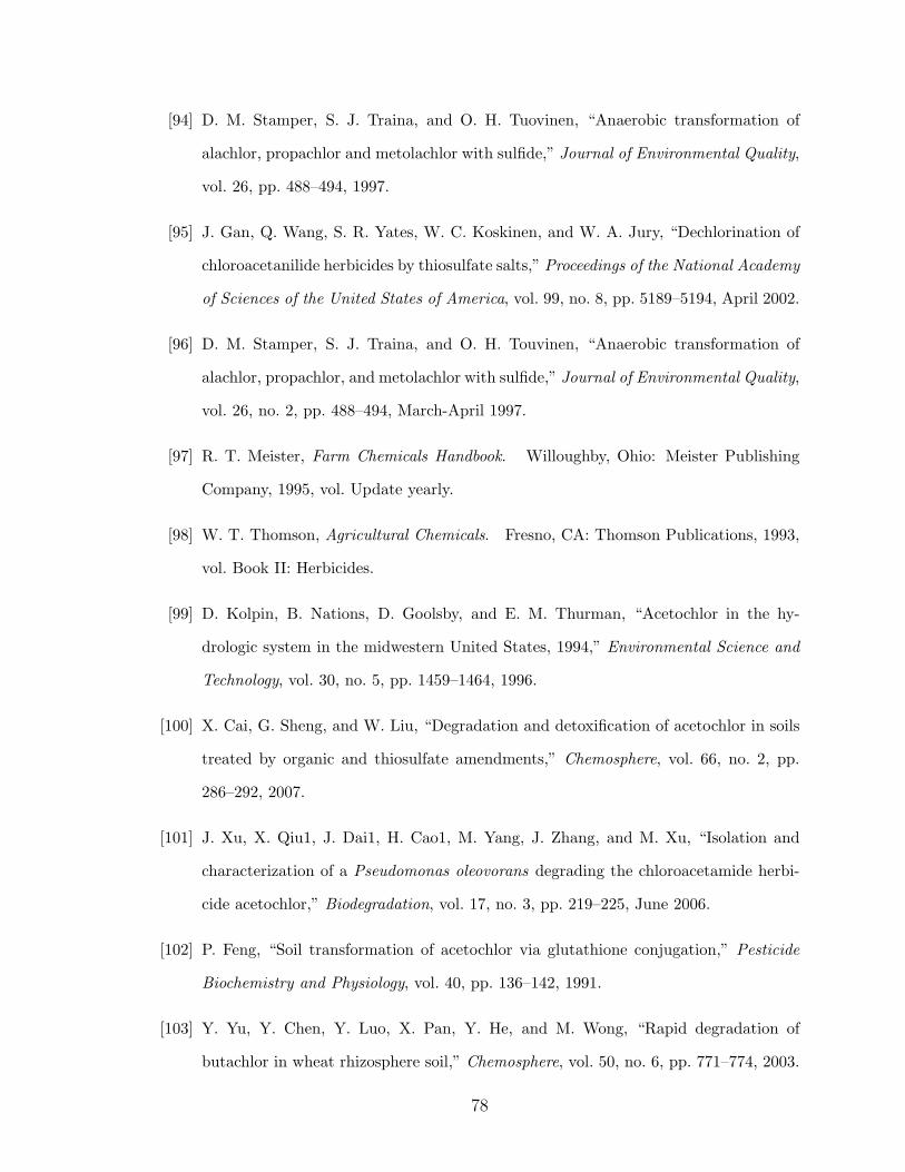
[94] D. M. Stamper, S. J. Traina, and O. H. Tuovinen, “Anaerobic transformation of
alachlor, propachlor and metolachlor with sulfide,” Journal of Environmental Quality,
vol. 26, pp. 488–494, 1997.
[95] J. Gan, Q. Wang, S. R. Yates, W. C. Koskinen, and W. A. Jury, “Dechlorination of
chloroacetanilide herbicides by thiosulfate salts,” Proceedings of the National Academy
of Sciences of the United States of America, vol. 99, no. 8, pp. 5189–5194, April 2002.
[96] D. M. Stamper, S. J. Traina, and O. H. Touvinen, “Anaerobic transformation of
alachlor, propachlor, and metolachlor with sulfide,” Journal of Environmental Quality,
vol. 26, no. 2, pp. 488–494, March-April 1997.
[97] R. T. Meister, Farm Chemicals Handbook. Willoughby, Ohio: Meister Publishing
Company, 1995, vol. Update yearly.
[98] W. T. Thomson, Agricultural Chemicals. Fresno, CA: Thomson Publications, 1993,
vol. Book II: Herbicides.
[99] D. Kolpin, B. Nations, D. Goolsby, and E. M. Thurman, “Acetochlor in the hy-
drologic system in the midwestern United States, 1994,” Environmental Science and
Technology, vol. 30, no. 5, pp. 1459–1464, 1996.
[100] X. Cai, G. Sheng, and W. Liu, “Degradation and detoxification of acetochlor in soils
treated by organic and thiosulfate amendments,” Chemosphere, vol. 66, no. 2, pp.
286–292, 2007.
[101] J. Xu, X. Qiu1, J. Dai1, H. Cao1, M. Yang, J. Zhang, and M. Xu, “Isolation and
characterization of a Pseudomonas oleovorans degrading the chloroacetamide herbi-
cide acetochlor,” Biodegradation, vol. 17, no. 3, pp. 219–225, June 2006.
[102] P. Feng, “Soil transformation of acetochlor via glutathione conjugation,” Pesticide
Biochemistry and Physiology, vol. 40, pp. 136–142, 1991.
[103] Y. Yu, Y. Chen, Y. Luo, X. Pan, Y. He, and M. Wong, “Rapid degradation of
butachlor in wheat rhizosphere soil,” Chemosphere, vol. 50, no. 6, pp. 771–774, 2003.
78

[104] R. Pal, P. Das, K. Chakrabarti, A. Chakraborty, and A. Chowdhury, “Butachlor
degradation in tropical soils: Effect of application rate, biotic-abiotic interactions and
soil conditions,” Journal of Environmental Science and Health, vol. 41, no. 7, pp. 1103
– 1113, October 2006.
[105] W. Erickson and L. Turner, “Metolachlor analysis of risks to endangered and threat-
ened salmon and steelhead,” Environmental Field Branch Office of Pesticide Pro-
grams, Tech. Rep., November 2002.
[106] T. Satapanajaru, S. D. Comfort, and P. J. Shea, “Enhancing metolachlor destruction
rates with aluminum and iron salts during zerovalent iron treatment,” Journal of
Environmental Quality, vol. 32, no. 5, p. 17261734, 2003.
[107] D. R. Shelton, S. Khader, J. S. Karns, and B. M. Pogell, “Metabolism of twelve
herbicides by streptomyces,” Biodegradation, vol. 7, no. 2, pp. 129–136, April 1996.
[108] S. Liu, M. Lu, and J. Bollag, “Transformation of metolachlor in soil inoculated with
a Streptomyces sp.” Biodegradation, vol. 1, no. 1, pp. 9–17, March 1991.
[109] S. Y. Liu, Z. Zheng, R. Zhang, and J. M. Bollag, “Sorption and metabolism of meto-
lachlor by a bacterial community,” Applied and Environmental Microbiology, vol. 55,
no. 3, p. 733740, March 1989.
[110] U. OPPTS, “Propachlor R.E.D.” Washington, D. C., Fact Sheet EPA-738-F-98-013,
November 1998.
[111] K. Barbalace, “Chemical database - propachlor,” EnvironmentalChemistry.com, 1995-
2007.
[112] W. H. Organization, “Environmental health criteria 147: Propachlor,” United Na-
tions Environment Programme, International Labour Organisation and World Health
Organization, Geneva, Report, 1993.
79

[113] M. Martin, E. Ferrer, R. Alonso, and J. Fernandez, “Bioremediation of soil con-
taminated by propachlor using native bacteria,” International Biodeterioration &
Biodegradation, vol. 35, pp. 213–225, 1995.
[114] W. Zheng, S. R. Yates, S. K. Papiernik, and M. Guo, “Transformation of herbicide
propachlorf by an agrochemical thiourea,” Environmental Science and Technology,
vol. 38, no. 24, pp. 6855–6860, December 2004.
[115] W. A. Battaglin, D. W. Kolpin, E. A. Scribner, K. M. Kuivila, and M. W. Sandstrom,
“Glyphosate, other herbicides, and transformation products in midwestern streams,
2002,” pp. 323–332, April 2005.
[116] B. Hartzler, “Amide wars ii: Sorting out the facts,” ISU Extension Agronomy, January
2000.
[117] Y. L. Yu, X. M. Wu, S. N. Li, H. F., H. Y. Zhan, and J. Q. Yu, “An exploration of the
relationship between adsorption and bioavailability of pesticides in soil to earthworm,”
Environmental Pollution, vol. 141, no. 3, pp. 428–433, 2006.
[118] K. S. Lee, K. K. Adhikary, H. W. Lee, B. Lee, and I. Lee, “Nucleophilic substitution
reactions of α-chloroacetanilides with benzylamines in dimethyl sulfoxide,” Organic
and Biomolecular Chemistry, vol. 1, pp. 1989–1994, 2003.
80

Appendix A
Rate Constants, Descriptor Values,
Correlation Plots
A.1 Bisulfide and Nitrate-reducing Rate Constants
The following data include the abiotic and biotic rate constants ([12] and [11]).
Table A.1: Bisulfide and biological rate reaction constants for chloroacetanilide herbicides
kHS−a kbio
b ln(kHS−) ln(kbio)
( Lmg HS−·hr
) ( Lmg V SS·hr
) ( Lmg HS−·hr
) ( Lmg V SS·hr
)
Alachlor 0.00160 0.00026 -6.43 -8.25Acetochlor 0.00112 0.00051 -6.79 -7.58Butachlor 0.00083 0.00052 -7.09 -7.56Metolachlor 0.00037 0.00027 -7.90 -8.22Propachlor 0.00255 0.00028 -5.97 -8.18aSource: Qin [12]bSource: Walker [11]
81

A.2 Descriptor Values
The following section includes descriptor values for the environmental fate parameters,
thermodynamic, atomic, steric, and electronic properties selected for the preliminary QSAR
analysis.
Table A.2: Descriptor Values
C-Cl Bond C=O Carbon log(Kow)b KHb Solubility
Energya Chargeb
(kJ/mole) (Mulliken) unitless unitless (mg/L)Alachlor 300.39 0.532 2.35 8.308 240Acetochlor 345.52 0.494 2.27 8.308 223Butachlor 355.51 0.483 3.63 7.939 23Metolachlor 355.78 0.464 3.31 8.185 520Propachlor 399.09 0.542 2.49 6.462 580aGaussian 03 R©bChem3D Pro 10.0 R©
Table A.3: Descriptor Values
CMAa CESVa Molecular Dipole C-Cl BondWeighta Momentb Lengthb
(A2) (A
3) (g/mole) (Debye) (A)
Alachlor 223.5 194.539 269.7671 2.9785 1.8956Acetochlor 227.156 195.461 269.7671 3.7384 1.89396Butachlor 263.768 229.504 311.84684 5.371 1.89496Metolachlor 229.513 212.621 283.79368 4.9036 1.89584Propachlor 179.665 152.858 211.68796 4.8607 1.89838aGaussian 03 R©bChem3D Pro 10.0 R©
82

A.3 Correlation Values between Descriptors and
Rate Constants
The tables below present the correlation values, R2, for the biotic/abiotic rate constants
and descriptors.
Table A.4: Correlations values between thermodynamic properties and rate constants
KH Solubility log(Kow) Molar Refractivity
units unitless (mg/L) unitless (cm3/mole)kHS- 0.61 0.12 0.39 0.74ln(kHS-) 0.37 0.00 0.47 0.52kbio 0.08 0.56 0.05 0.27ln(kbio) 0.07 0.54 0.05 0.26
Table A.5: Correlations values between atomic, electronic and steric descriptors and rateconstants
C-Cl C-Cl C=O Dipole CESV CMA MW
Bond Bond Carbon MomentLength Energy Charge
units A (kJ/mole) (Mulliken) (Debye) (A3) (A
2) (g/mole)
kHS- 0.50 0.11 0.91 0.04 0.81 0.64 0.75ln(kHS-) 0.22 0.02 0.91 0.12 0.60 0.39 0.50kbio 0.46 0.00 0.16 0.05 0.23 0.38 0.27ln(kbio) 0.44 0.00 0.16 0.05 0.22 0.36 0.25
83

A.4 Correlation Plots
84

k HS-
vs.
log(
K ow)
y =
-0.
0008
x +
0.0
037
R2
= 0
.393
8
0.00
000
0.00
050
0.00
100
0.00
150
0.00
200
0.00
250
0.00
300
0.00
350
0.00
400
22.
53
3.5
44.
5
log(
Kow
)
kHS- (L/mg HS-•hr)
Figure A.1: kHS− and ln(Kow) correlation plot.
85

ln(k
HS-
) vs
. lo
g(K o
w)
y =
-0.
8029
x -
4.58
38
R2
= 0
.466
8
-9
-8.5-8
-7.5-7
-6.5-6
-5.5-5
-4.5-4
22.
53
3.5
44.
5
log(
Kow
)
ln(kHS-) (L/mg HS-•hr)
Figure A.2: ln(kHS−) and ln(Kow) correlation plot.
86

k bio v
s. lo
g(K o
w)
y =
5E
-05x
+ 0
.000
2
R2
= 0
.053
4
0
0.00
01
0.00
02
0.00
03
0.00
04
0.00
05
0.00
06
22.
53
3.5
44.
55
log(
Kow
)
kbio (L/mg VSS•hr)
Figure A.3: kbio and ln(Kow) correlation plot.
87

ln(k
bio)
vs.
log(
K ow)
y =
0.1
307x
- 8
.326
4
R2
= 0
.051
8
-8.4
-8.3
-8.2
-8.1-8
-7.9
-7.8
-7.7
-7.6
-7.5
22.
53
3.5
44.
5
log(
Kow
)
ln(kbio) (L/mg VSS•hr)
Figure A.4: ln(kbio) and ln(Kow) correlation plot.
88

k HS-
vs.
Hen
ry's
Co
nsta
nt,
K H
y =
-0.
0008
x +
0.0
078
R2
= 0
.605
4
0.00
000
0.00
050
0.00
100
0.00
150
0.00
200
0.00
250
0.00
300
66.
57
7.5
88.
5
KH (
unitl
ess)
kHS- (L/mg HS-•hr)
Figure A.5: kHS− and KH correlation plot.
89

ln(k
HS-
) vs
. H
enry
's C
ons
tant
, K H
y =
-0.
5591
x -
2.45
66
R2
= 0
.365
2
-8.5-8
-7.5-7
-6.5-6
-5.5-5
66.
57
7.5
88.
5
KH (
unitl
ess)
ln(kHS-) (L/mg HS-•hr)
Figure A.6: ln(kHS−) and KH correlation plot.
90
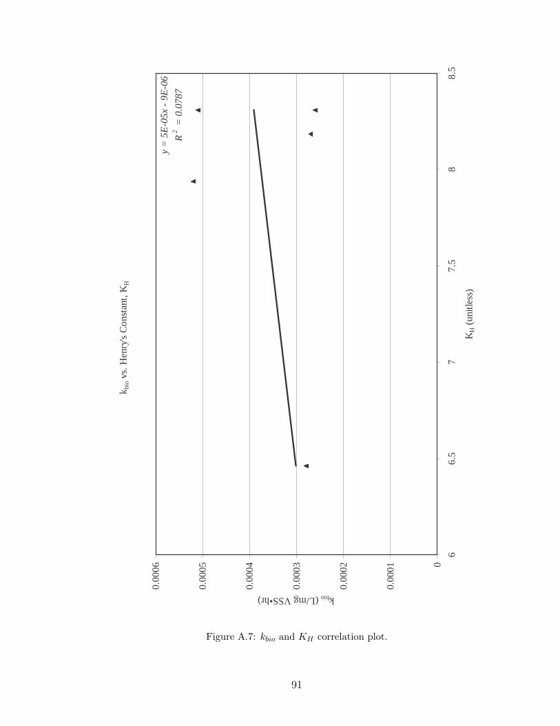
k bio v
s. H
enry
's C
ons
tant
, K H
y =
5E
-05x
- 9
E-0
6
R2
= 0
.078
7
0
0.00
01
0.00
02
0.00
03
0.00
04
0.00
05
0.00
06
66.
57
7.5
88.
5
KH (
unitl
ess)
kbio (L/mg VSS•hr)
Figure A.7: kbio and KH correlation plot.
91

ln(k
bio)
vs.
Hen
ry's
Co
nsta
nt,
K H
y =
0.1
193x
- 8
.894
7
R2
= 0
.069
7
-8.4
-8.2-8
-7.8
-7.6
-7.4
-7.2-7
66.
57
7.5
88.
5
KH (
unitl
ess)
ln(kbio) (L/mg VSS•hr)
Figure A.8: ln(kbio) and KH correlation plot.
92

k HS-
vs.
So
lubi
lity
y =
1E
-06x
+ 0
.000
9
R2
= 0
.115
5
0.00
000
0.00
050
0.00
100
0.00
150
0.00
200
0.00
250
0.00
300
010
020
030
040
050
060
070
0
So
lubi
lity
(mg/
L)
kHS- (L/mg HS-•hr)
Figure A.9: kHS− and solubility correlation plot.
93

ln(k
HS-
) vs
. S
olu
bilit
y
y =
0.0
002x
- 6
.901
6
R2
= 0
.003
8
-8.5-8
-7.5-7
-6.5-6
-5.5-5
-4.5-4
010
020
030
040
050
060
070
0
So
lubi
lity
(mg/
L)
ln(kHS-) (L/mg HS-•hr)
Figure A.10: ln(kHS−) and solubility correlation plot.
94

k bio v
s. S
olu
bilit
y
y =
-4E
-07x
+ 0
.000
5
R2
= 0
.563
6
0
0.00
01
0.00
02
0.00
03
0.00
04
0.00
05
0.00
06
010
020
030
040
050
060
070
0
So
lubi
lity
(mg/
L)
kbio (L/mg VSS•hr)
Figure A.11: kbio and solubility correlation plot.
95
ln(k
bio)
vs.
So
lubi
lity
y =
-0.
0011
x -
7.59
97
R2
= 0
.542
5
-8.3
-8.2
-8.1-8
-7.9
-7.8
-7.7
-7.6
-7.5
010
020
030
040
050
060
070
0
So
lubi
lity
(mg/
L)
ln(kbio) (L/mg VSS•hr)
Figure A.12: ln(kbio) and solubility correlation plot.
96

k HS-
vs.
Mo
lar
Ref
ract
ivity
y =
-0.
0000
66x
+ 0
.006
227
R2
= 0
.743
986
0.00
000
0.00
100
0.00
200
0.00
300
0.00
400
0.00
500
0.00
600
0.00
700 50
5560
6570
7580
8590
Mo
lar
Ref
ract
ivity
(cm
3 /mo
le)
kHS- (L/mg HS-•hr)
Figure A.13: kHS− and molar refractivity correlation plot.
97
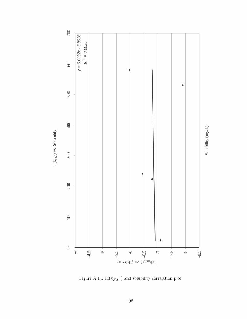
ln(k
HS-
) vs
. S
olu
bilit
y
y =
0.0
002x
- 6
.901
6
R2
= 0
.003
8
-8.5-8
-7.5-7
-6.5-6
-5.5-5
-4.5-4
010
020
030
040
050
060
070
0
So
lubi
lity
(mg/
L)
ln(kHS-) (L/mg HS-•hr)
Figure A.14: ln(kHS−) and solubility correlation plot.
98

k bio v
s. M
ola
r R
efra
ctiv
ity
y =
0.0
0000
6x -
0.0
0011
4
R2
= 0
.272
095
0
0.00
01
0.00
02
0.00
03
0.00
04
0.00
05
0.00
06
5055
6065
7075
8085
9095
Mo
lar
Ref
ract
ivity
(cm
3 /mo
le)
kbio (L/mg VSS•hr)
Figure A.15: kbio and molar refractivity correlation plot.
99

ln(k
bio)
vs.
Mo
lar
Ref
ract
ivity
y =
0.0
166x
- 9
.196
2
R2
= 0
.257
3
-8.4
-8.2-8
-7.8
-7.6
-7.4
-7.2-7
5560
6570
7580
8590
9510
0
Mo
lar
Ref
ract
ivity
(cm
3 /mo
le)
ln(kbio) (L/mg VSS•hr)
Figure A.16: ln(kbio) and molar refractivity correlation plot.
100

k HS-
vs.
Mo
lecu
lar
Wei
ght
y =
-0.
0000
20x
+ 0
.006
613
R2
= 0
.751
384
0.00
000
0.00
050
0.00
100
0.00
150
0.00
200
0.00
250
0.00
300
0.00
350
0.00
400
0.00
450
0.00
500 15
017
019
021
023
025
027
029
031
033
0
Mo
lecu
lar
Wei
ght
(g/m
ole
)
kHS- (L/mg HS-•hr)
Figure A.17: kHS− and molecular weight correlation plot.
101

ln(k
HS-
) vs
. S
olu
bilit
y
y =
0.0
002x
- 6
.901
6
R2
= 0
.003
8
-8.5-8
-7.5-7
-6.5-6
-5.5-5
-4.5-4
010
020
030
040
050
060
070
0
So
lubi
lity
(mg/
L)
ln(kHS-) (L/mg HS-•hr)
Figure A.18: ln(kHS−) and solubility correlation plot.
102

k bio v
s. M
ole
cula
r W
eigh
t
y =
0.0
0000
2x -
0.0
0014
3
R2
= 0
.266
001
0
0.00
01
0.00
02
0.00
03
0.00
04
0.00
05
0.00
06
200
220
240
260
280
300
320
340
Mo
lecu
lar
Wei
ght
(g/m
ole
)
kbio (L/mg VSS•hr)
Figure A.19: kbio and molecular weight correlation plot.
103

ln(k
bio)
vs.
Mo
lecu
lar
Wei
ght
y =
0.0
049x
- 9
.269
5
R2
= 0
.250
7
-9.5-9
-8.5-8
-7.5-7
-6.5-6
200
220
240
260
280
300
320
340
Mo
lecu
lar
Wei
ght
(g/m
ole
)
ln(kbio) (L/mg VSS•hr)
Figure A.20: ln(kbio) and molecular weight correlation plot.
104

k HS-
vs.
Co
nno
lly M
ole
cula
r A
rea
y =
-2E
-05x
+ 0
.006
3
R2
= 0
.643
3
0.00
000
0.00
050
0.00
100
0.00
150
0.00
200
0.00
250
0.00
300 15
017
019
021
023
025
027
0
Co
nno
lly M
ole
cula
r A
rea
(Å2 )
kHS- (L/mg HS-•hr)
Figure A.21: kHS− and Connolly molecular area correlation plot.
105

ln(k
HS-
) vs
. C
onn
olly
Mo
lecu
lar
Are
a
y =
-0.
0152
x -
3.42
29
R2
= 0
.392
8
-8.5-8
-7.5-7
-6.5-6
-5.5-5
-4.5
150
170
190
210
230
250
270
Co
nno
lly M
ole
cula
r A
rea
(Å2 )
ln(kHS-) (L/mg HS-•hr)
Figure A.22: ln(kHS−) and Connolly molecular area correlation plot.
106

k bio v
s. C
onn
olly
Mo
lecu
lar
Are
a
y =
3E
-06x
- 0
.000
3
R2
= 0
.378
8
0
0.00
01
0.00
02
0.00
03
0.00
04
0.00
05
0.00
06
0.00
07
150
170
190
210
230
250
270
Co
nno
lly M
ole
cula
r A
rea
(Å2 )
kbio (L/mg VSS•hr)
Figure A.23: kbio and Connolly molecular area correlation plot.
107

ln(k
bio)
vs.
Co
nno
lly M
ole
cula
r A
rea
y =
0.0
071x
- 9
.560
5
R2
= 0
.361
3
-8.4
-8.2-8
-7.8
-7.6
-7.4
-7.2-7
150
170
190
210
230
250
270
Co
nno
lly M
ole
cula
r A
rea
(Å2 )
ln(kbio) (L/mg VSS•hr)
Figure A.24: ln(kbio) and Connolly molecular area correlation plot.
108

k HS-
vs.
Co
nno
lly E
xclu
ded
So
lven
t V
olu
me
y =
-3E
-05x
+ 0
.006
5
R2
= 0
.808
9
0.00
000
0.00
050
0.00
100
0.00
150
0.00
200
0.00
250
0.00
300 14
015
016
017
018
019
020
021
022
023
024
0
Co
nno
lly E
xclu
ded
So
lven
t V
olu
me(
Å3 )
kHS- (L/mg HS-•hr)
Figure A.25: kHS− and Connolly excluded solvent volume correlation plot.
109

ln(k
HS-
) vs
. C
onn
olly
Exc
lude
d S
olv
ent
Vo
lum
e
y =
-0.
0197
x -
2.95
52
R2
= 0
.600
3
-8.5-8
-7.5-7
-6.5-6
-5.5-5
-4.5-4
140
150
160
170
180
190
200
210
220
230
240
Co
nno
lly E
xclu
ded
So
lven
t V
olu
me
(Å3 )
ln(kHS-) (L/mg HS-•hr)
Figure A.26: ln(kHS−) and Connolly excluded solvent volume correlation plot.
110

k bio v
s. C
onn
olly
Exc
lude
d S
olv
ent
Vo
lum
e
y =
2E
-06x
- 8
E-0
5
R2
= 0
.228
9
0
0.00
01
0.00
02
0.00
03
0.00
04
0.00
05
0.00
06
140
150
160
170
180
190
200
210
220
230
240
Co
nno
lly E
xclu
ded
So
lven
t V
olu
me
(Å3 )
kbio (L/mg VSS•hr)
Figure A.27: kbio and Connolly excluded solvent volume correlation plot.
111

ln(k
bio)
vs.
Co
nno
lly E
xclu
ded
So
lven
t V
olu
me
y =
0.0
058x
- 9
.097
R2
= 0
.215
7
-8.5
-8.3
-8.1
-7.9
-7.7
-7.5
-7.3
140
150
160
170
180
190
200
210
220
230
240
Co
nno
lly E
xclu
ded
So
lven
t V
olu
me
(Å3 )
ln(kbio) (L/mg VSS•hr)
Figure A.28: ln(kbio) and Connolly excluded solvent volume correlation plot.
112

k HS-
vs.
Dip
ole
Mo
men
t
y =
-0.
0002
x +
0.0
02
R2
= 0
.040
3
0.00
000
0.00
050
0.00
100
0.00
150
0.00
200
0.00
250
0.00
300 2.
53
3.5
44.
55
5.5
6
Dip
ole
Mo
men
t (D
ebye
)
kHS- (L/mg HS-•hr)
Figure A.29: kHS− and dipole moment correlation plot.
113

ln(k
HS-
) vs
. D
ipo
le M
om
ent
y =
-0.
2546
x -
5.72
73
R2
= 0
.118
6
-8.5-8
-7.5-7
-6.5-6
-5.5-5
-4.5-4
2.5
33.
54
4.5
55.
56
Dip
ole
Mo
men
t (D
ebye
)
kHS- (L/mg HS-•hr)
Figure A.30: ln(kHS−) and dipole moment correlation plot.
114

k bio v
s. D
ipo
le M
om
ent
y =
3E
-05x
+ 0
.000
2
R2
= 0
.049
3
0
0.00
01
0.00
02
0.00
03
0.00
04
0.00
05
0.00
06
2.5
33.
54
4.5
55.
56
Dip
ole
Mo
men
t (D
ebye
)
kbio (L/mg VSS•hr)
Figure A.31: kbio and dipole moment correlation plot.
115
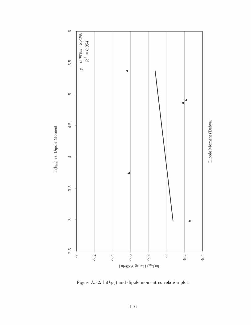
ln(k
bio)
vs.
Dip
ole
Mo
men
t
y =
0.0
839x
- 8
.325
9
R2
= 0
.054
-8.4
-8.2-8
-7.8
-7.6
-7.4
-7.2-7
2.5
33.
54
4.5
55.
56
Dip
ole
Mo
men
t (D
ebye
)
ln(kbio) (L/mg VSS•hr)
Figure A.32: ln(kbio) and dipole moment correlation plot.
116

k HS-
vs.
C-C
l Bo
nd L
engt
h
y =
0.3
575x
- 0
.676
4
R2
= 0
.497
1
0.00
000
0.00
050
0.00
100
0.00
150
0.00
200
0.00
250
0.00
300 1.89
351.
894
1.89
451.
895
1.89
551.
896
1.89
651.
897
1.89
751.
898
1.89
851.
899
C-C
l Bo
nd L
engt
h (Å
)
kHS- (L/mg HS-•hr)
Figure A.33: kHS− and C-Cl bond length correlation plot.
117

ln(k
HS-
) vs
. C
-Cl B
ond
Len
gth
y =
208
.52x
- 4
02.1
4
R2
= 0
.222
-8.5-8
-7.5-7
-6.5-6
-5.5-5
-4.5-41.
8935
1.89
41.
8945
1.89
51.
8955
1.89
61.
8965
1.89
71.
8975
1.89
81.
8985
1.89
9
C-C
l Bo
nd L
engt
h (Å
)
ln(kHS-) (L/mg HS-•hr)
Figure A.34: ln(kHS−) and C-Cl bond length correlation plot.
118

k bio v
s. C
-Cl B
ond
Len
gth
y =
-0.
0555
x +
0.1
056
R2 =
0.4
596
0
0.00
01
0.00
02
0.00
03
0.00
04
0.00
05
0.00
06 1.89
351.
894
1.89
451.
895
1.89
551.
896
1.89
651.
897
1.89
751.
898
1.89
851.
899
C-C
l Bo
nd L
engt
h (Å
)
kbio (L/mg VSS•hr)
Figure A.35: kbio and C-Cl bond length correlation plot.
119

ln(k
bio)
vs.
C-C
l Bo
nd L
engt
h
y =
-14
4.06
x +
265
.14
R2
= 0
.443
7
-8.4
-8.3
-8.2
-8.1-8
-7.9
-7.8
-7.7
-7.6
-7.51.
8935
1.89
41.
8945
1.89
51.
8955
1.89
61.
8965
1.89
71.
8975
1.89
81.
8985
1.89
9
C-C
l Bo
nd L
engt
h (Å
)
ln(kbio) (L/mg VSS•hr)
Figure A.36: ln(kbio) and C-Cl bond length correlation plot.
120

k HS-
vs.
C-C
l Bo
nd E
nerg
y
y =
8E
-06x
- 0
.001
5
R2
= 0
.113
0.00
000
0.00
050
0.00
100
0.00
150
0.00
200
0.00
250
0.00
300 25
027
029
031
033
035
037
039
041
0
C-C
l Bo
nd E
nerg
y (k
J/m
ole
)
kHS- (L/mg HS-•hr)
Figure A.37: kHS− and C-Cl bond energy correlation plot.
121

ln(k
HS-
) vs
. C
-Cl B
ond
Ene
rgy
y =
0.0
03x
- 7.
9
R2
= 0
.021
3
-8.5-8
-7.5-7
-6.5-6
-5.5-5
-4.5-4
270
290
310
330
350
370
390
410
C-C
l Bo
nd E
nerg
y (k
J/m
ole
)
ln(kHS-) (L/mg HS-•hr)
Figure A.38: ln(kHS−) and C-Cl bond energy correlation plot.
122

k bio v
s. C
-Cl B
ond
Ene
rgy
y =
1E
-07x
+ 0
.000
3
R2
= 0
.001
3
0
0.00
01
0.00
02
0.00
03
0.00
04
0.00
05
0.00
06
290
310
330
350
370
390
410
C-C
l Bo
nd E
nerg
y (k
J/m
ole
)
kbio (L/mg VSS•hr)
Figure A.39: kbio and C-Cl bond energy correlation plot.
123

ln(k
bio)
vs.
C-C
l Bo
nd E
nerg
y
y =
0.0
006x
- 8
.157
7
R2 =
0.0
031
-8.3
-8.2
-8.1-8
-7.9
-7.8
-7.7
-7.6
-7.5
290
310
330
350
370
390
410
C-C
l Bo
nd E
nerg
y (k
J/m
ole
)
ln(kbio) (L/mg VSS•hr)
Figure A.40: ln(kbio) and C-Cl bond energy correlation plot.
124

k HS-
vs.
Car
bony
l Car
bon
Cha
rge
y =
0.0
24x
- 0.
0108
R2
= 0
.907
4
0.00
000
0.00
050
0.00
100
0.00
150
0.00
200
0.00
250
0.00
300 0.
460.
470.
480.
490.
50.
510.
520.
530.
540.
55
Car
bony
l Car
bon
Cha
rge
(Mul
liken
)
kHS- (L/mg HS-•hr)
Figure A.41: kHS− and C=O carbon charge correlation plot.
125

ln(k
HS-
) vs
. C
arbo
nyl C
arbo
n C
harg
e
y =
20.
995x
- 1
7.4
R2
= 0
.911
5
-8.5-8
-7.5-7
-6.5-6
-5.5-5
-4.5-4
0.46
0.47
0.48
0.49
0.5
0.51
0.52
0.53
0.54
0.55
Car
bony
l Car
bon
Cha
rge
(Mul
liken
)
ln(kHS-) (L/mg HS-•hr)
Figure A.42: ln(kHS−) and C=O carbon charge correlation plot.
126

k bio v
s. C
arbo
nyl C
arbo
n C
harg
e
y =
-0.
0016
x +
0.0
012
R2
= 0
.158
0
0.00
01
0.00
02
0.00
03
0.00
04
0.00
05
0.00
06
0.46
0.47
0.48
0.49
0.5
0.51
0.52
0.53
0.54
0.55
Car
bony
l Car
bon
Cha
rge
(Mul
liken
)
kbio (L/mg VSS•hr)
Figure A.43: kbio and C=O carbon charge correlation plot.
127

ln(k
bio)
vs.
Car
bony
l Car
bon
Cha
rge
y =
-4.
2411
x -
5.82
58
R2
= 0
.155
8
-8.3
-8.2
-8.1-8
-7.9
-7.8
-7.7
-7.6
-7.5
0.46
0.47
0.48
0.49
0.5
0.51
0.52
0.53
0.54
0.55
Car
bony
l Car
bon
Cha
rge
(Mul
liken
)
ln(kbio) (L/mg VSS•hr)
Figure A.44: ln(kbio) and C=O carbon charge correlation plot.
128

A.5 Molecular Mechanics Figures
Figure A.45: Alachlor before energy minimization.
Figure A.46: Alachlor after energy minimization.
129

Figure A.47: Acetochlor before energy minimization.
Figure A.48: Acetochlor after energy minimization.
130

Figure A.49: Butachlor before energy minimization.
Figure A.50: Butachlor after energy minimization.
131

Figure A.51: Metolachlor before energy minimization.
Figure A.52: Metolachlor after energy minimization.
132

Figure A.53: Propachlor before energy minimization.
Figure A.54: Propachlor after energy minimization.
133

VITA
Angela Robyn Kana
Candidate for the Degree of
Master of Science
Thesis: QUANTITATIVE STRUCTURE-ACTIVITY RELATIONSHIP:PREDICTION OF ANAEROBIC TRANSFORMATION OFCHLOROACETANILIDE HERBICIDES
Major Field: Environmental Engineering
Biographical:
Personal Data: Born in Daegu, South Korea on September 13, 1982, the daughterof John and Ginger Kana.
Education: Received Bachelor of Science degree in Civil and Environmental Engi-neering from Oklahoma State University, Stillwater, Oklahoma in May 2005.Completed the requirements for the Master of Science degree with a major inEnvironmental Engineering at Oklahoma State University in July 2007.
Experience: Employed by Oklahoma State University, School of Civil and Environ-mental Engineering as an undergraduate and graduate assistant, Fall 2004 topresent.
Professional Memberships: Chi Epsilon, Tau Beta Pi, Phi Kappa Phi, Phi Eta Sigma,ASCE

Name: Angela Kana Date of Degree: July, 2007
Institution: Oklahoma State University Location: Stillwater, Oklahoma
Title of Study: QUANTITATIVE STRUCTURE-ACTIVITY RELATIONSHIP:PREDICTION OF ANAEROBIC TRANSFORMATION OFCHLOROACETANILIDE HERBICIDES
Pages in Study: 133 Candidate for the Degree of Master of Science
Major Field: Environmental Engineering
Scope and Method of Study: The purpose of this work is to perform a preliminaryanalysis for future use in a full-scale quantitative structure-activity relationship(QSAR) analysis to ultimately predict the anaerobic transformation rates ofchloroacetanilide herbicides with bisulfide and denitrifying bacteria and to elu-cidate degradation mechanisms and pathways. Chem Draw 10.0 R©, Chem3D Pro10.0 R©, and Gaussian 03 R©were chemical software programs used to compute the dataused in the statistical analysis of this study.
Findings and Conclusions: A preliminary analysis of quantitative structure-activity re-lationships was conducted over five selected chloroacetanilide herbicides: alachor,acetochlor, butachlor, metolachlor, and propachlor. Multiple structural, thermody-namic, atomic, electronic and steric descriptors were examined in regards to theircorrelations with nitrate-reducing rate constants and bisulfide reaction rate constants.Experimental results suggested there are various potential descriptors to predict theactivity of these herbicides with bisulfide. Most notably, the descriptors carbonyl-carbon charge, Connolly excluded solvent volume, and molecular weight displayedthe highest correlations for the bisulfide reaction. A limited number of descriptorswere found to correlate well with the nitrate-reducing rate constants. Future areas ofresearch might include further laboratory testing of descriptors, additional chloroac-etanilides to examine, and testing to isolate denitrifying bacteria capable of degradingthese herbicides.
Advisor’s Approval:Dr. Gregory Wilber