Quantity Discounts and Capital Misallocation

in Vertical Relationships∗

Ken Onishi†

January 2014

Job Market Paper

Abstract

I study transactions between aircraft manufacturers and airlines as well as airlines’ uti-

lization of their fleet. Aircraft production is characterized by economies of scale via learning-

by-doing, which creates a trade-off between current profit and future competitive advantage

in the aircraft market. The latter consideration makes large buyers more attractive than

small buyers and induces quantity discounts. The resulting nonlinear pricing strategy may

distort both production and allocation in favor of large buyers. There is a negative correlation

between the size of aircraft orders and the per-unit price. There is also a positive correlation

between the price paid and the utilization rate of the aircraft model, which suggests that the

manufacturers’ price discrimination leads to the misallocation of aircraft. To assess whether

there is an inefficient allocation, I model the market and show that price discrimination by

upstream firms may lead to an inefficient outcome compared with uniform pricing. Then,

I construct and estimate a dynamic model of the aircraft market that includes a model of

utilization. Finally, I conduct counterfactual simulations using the estimated parameters. I

find that uniform pricing increases aircraft production by 10% and total welfare by 1.6%.

∗I am extremely thankful to Igal Hendel, David Besanko, Aviv Nevo, Rob Porter and seminar participants atNorthwestern University for their valuable comments and suggestions.

†Northwestern University, Department of Economics. email: onishi@u.northwestern.edu

1

1 Introduction

Most economic activities involve vertical relationships where upstream firms supply capital/intermediate

goods to downstream firms and downstream firms supply final goods to consumers. In upstream

markets, price discrimination is common and affects competition in downstream markets via capi-

tal allocation. Though price discrimination in upstream markets may have a large impact in both

upstream and downstream markets, whether capital is efficiently produced and allocated in vertical

relationships has been an open empirical question.

In this paper, I study the welfare consequence of price discrimination in the aircraft market

using detailed data on aircraft transactions and aircraft utilization. The richness in the data allows

me to study the connection between the vertical relationship in the aircraft (upstream) market

and productivity in the airline (downstream) market. I construct and estimate a model of the

industries in which competition and economies of scale in production lead to price discrimination in

the aircraft market with higher discounts to larger buyers. The existence of quantity discounts may

distort both production and allocation and leave room for improving social welfare from the policy

maker’s point of view. For a fixed production amount of aircraft, social welfare and productivity

improve in the airline market with aircraft reallocation. Also, potential policy interventions, such

as forcing manufacturers to post a uniform price, may induce more-intense competition and help

restore efficiency in aircraft production.

To motivate the model, I first present a set of descriptive regressions. In the data, I find evidence

that manufactures are exercising quantity discounts, in which airlines that buy large quantities

pay less for each unit of aircraft. Also, I find evidence that airlines paying less for each unit utilize

the aircraft less. The positive correlation between the price paid and the utilization rate suggests

misallocation. The utilization rate indicates the marginal profitability or operational efficiency of

the airline. From the social planner’s point of view, more aircraft should be allocated to airlines

with higher marginal profitability or higher marginal operational efficiency. On the other hand,

the data suggest that aircraft are not allocated according to marginal profitability. Rather, the

data suggest that airlines with lower marginal profitability face a lower aircraft unit price and,

therefore, have easier access to the marginal aircraft, which causes inefficiency with misallocation.

2

One possible explanation for the source of inefficiency is the existence of economies of scale

on the supply side. As pointed out in the existing literature, aircraft production is characterized

by a learning-by-doing effect. The learning-by-doing effect creates a trade-off between the current

profit and future intensity of competition. By lowering the current price aggressively, aircraft

manufactures can attract more orders, which translates into a lower marginal cost in the future.

To lower future competition intensity, buyers with larger orders are more attractive than buyers

with small orders. Serving a large buyer reduces the manufacturer’s own future marginal cost

through the learning-by-doing effect and, at the same time, takes away the opponent’s opportunity

to reduce the future marginal cost. This effect creates the incentive to strategically serve large

buyers by offering a quantity discount. If the quantity discount is a consequence of supply-side

factors, the allocation of aircraft may create inefficiency because a large buyer receives a more

favorable price than a small buyer for the marginal unit, even though the small buyer is willing to

pay more than the large buyer.

In this paper, I first construct a simple model to show that the existence of economies of scale

together with competition among manufacturers may induce quantity discounts and misallocation.

The intuition of the result is simple. To reduce future competition intensity, manufacturers compete

for the large buyer, which distorts both production and allocation. In the model, forcing uniform

pricing increases both production and total welfare. By forcing uniform pricing, manufacturers

do not compete by making a favorable offer to the large buyer but simply by producing more.

Intuitively, policy makers can force manufacturers to compete with equal intensity for all buyers,

which may result in higher overall competition intensity and help increase total welfare.

Indeed, if the good is capital, the model can explain the pattern in the data. Suppose the capital

is used in final-good production where the production function is characterized by the amount

of capital and the utilization rate. Also, suppose there is a cost associated with utilization. To

maximize profit, final-good producers determine the amount of capital and utilization rate using

the relative marginal factor price of capital and utilization. Therefore, final-good producers facing

a lower price of capital substitute capital for utilization, and those facing a higher price do the

opposite, which creates a positive correlation between the capital price and utilization rate.

3

In the estimation, I build a dynamic model with economies of scale in production and multidi-

mensional heterogeneity—heterogeneity in profitability and ease of investment—in airlines, where

manufacturers propose price menu as a function of product quantity and airline characteristics.

Manufacturers use the price menu to price discriminate among airlines and screen the ease of in-

vestment within airlines, which may create inefficiency. The object of interest in the estimation is

the parameter on the airlines’ utilization model and the aircraft production model. The parameter

on the utilization model and the heterogeneity in profitability among airlines are identified from the

variation in the utilization rate. As Gavazza (2011) and other papers on capital productivity note,

productivity and the capital utilization rate are closely tied and often indistinguishable. In the

model, there is a one-to-one correspondence between profitability and the utilization rate, which

allows for the identification of airlines’ profitability from the data. The supply-side parameter is

identified from the pricing optimality and variation across time. By estimating the dynamic model

of supply and demand, the static marginal cost of production is identified. Then, by relating

the static marginal cost to cumulative production, the marginal cost, as a function of cumulative

production, can be identified.

In the counterfactual analysis, I quantify the welfare loss caused by misallocation and evaluate

the effectiveness of potential policy interventions. I find that forcing manufacturers to post a single

uniform price increases aircraft production by 11% and total welfare by 1.6%, which suggests that

the intuition from the theoretical example still holds in the structrual model of the industry. I

also compare the result under “Grand Menu Pricing” regulation, where manufacturers are forced

to post a price menu that only depends on the quantity but not on airline characteristics. “Grand

Menu Pricing” allows manufacturers to price discriminate airlines by nonlinear pricing, which may

incrase aircraft production by screening airlines in the dimension of ease of investment. In fact, I

find that “Grand Menu Pricing” regulation increases aircraft production by 10% and total welfare

by 3.3%.

4

2 Literature

This paper is related to several strands of the literature. First, this study is related to the literature

on input misallocation. Input reallocation has been understood as an important drive force of

aggregate TFP growth. Restuccia and Rogerson (2008) and Hsieh and Klenow (2009) estimate

that about 30% to 60% higher aggregate TFP growth can be achieved by input reallocation. As is

pointed out in the literature, one source of misallocation is input price dispersion.1 In this paper,

I study the implication of input price dispersion resulted from price discrimination in vertical

relationships.

Another important literature that the paper contributes to is the literature on non-linear pricing

and vertical relationships. The screening aspect of the non-linear pricing has been extensively

studied. Stole (1995) shows that second degree price discrimination is sustainable even in a multi-

firm setting. There are number of papers including Rochet and Stole (2002) and Armstrong and

Vickers (2010) that further explore the role of non-linear pricing under oligopoly. In contrast to

the intense study of theoretical implication, little is known empirically. Busse and Rysman (2005)

documents the relationship between competition and the curvature of the price-quantity menu.

Another important aspect of non-linear pricing arise in vertical relationships between upstream

and downstream firms. The primary interest is to identify if the firms use non-linear pricing to avoid

double marginalization. Villas-Boas (2002) establishes an estimation and inference method from

market level data. However, the actual transaction data is still ideally needed to understand the

precise structure of the market. Mortimer (2008) investigates the welfare implication of revenue

sharing between upstream and downstream firms using the actual contracts in the video rental

industry. In particular, this paper is closely related to the literature on the size-related buyers’

purchasing power. There is a growing literature on the buyer-size effect on price discounts. A

number of theoretical papers including Chipty and Snyder (1999), Snyder (1996) and Gans and

King (2002) shows the upstream competition may lead to quantity discounts. Ellison and Snyder

(2010) empirically shows that buyer-size effect on price discounts appears only under upstream

competition and there is no quantity discounts if the upstream firm is a monopolist. Sorensen

1Foster, Haltiwanger, and Syverson (2008) points out that not only input but also output price dispersion is animportant factor to understand the productivity growth and reallocation.

5

(2003) studies the transaction price between hospitals and insurers, and identifies the buyer size

as a source of the price discount. The findings in this paper are consistent with the literature.

Furthermore, I identify a new mechanism that induces quantity discounts and potential inefficiency.

The third strand of the literature to which this paper is related is the literature on the learning-

by-doing. The empirical study of the learning-by-doing starts in engineering as early as Wright

(1936) in the aircraft production industry. The learning-by-doing effect attracted intense research

interest in economics, too. Spence (1981) analyzes the theoretical aspects of the relationship

between the learning curve and competition. Fudenberg and Tirole (1983) analyzes the market

performance and strategic incentives in a model with a learning-by-doing effect. Cabral and

Riordan (1994) analyzes the strategic incentive coming from the learning-by-doing effect in a

differentiated good market where two firms compete by setting price, and shows the possibility of

predatory pricing. In addition to the theoretical literature, there is a growing body of work on

the estimation of the learning effects. Thornton and Thompson (2001) estimates the effect of the

learning-by-doing in the wartime shipbuilding industry and Ohashi (2005) evaluates the efficiency

gain from the government subsidy in the Japanese steel industry. Paired with the learning-by-

doing, organizational forgetting also attracted economists’ attention. Benkard (2000), Levitt,

List, and Syverson (2012) and Thompson (2007), among other papers, find empirical evidence

that there exists a learning-and-forgetting, and Benkard (2004) estimates a model for commercial

aircrafts with dynamic aspects of the learning-and-forgetting. Besanko, Dorazelski, Kryukov, and

Satterthwaite (2010) conducts detailed analysis of the industry dynamics with a learning-and-

forgetting effect and concludes the existence of the learning-and-forgetting increase the incentive

to price more aggressively than the industries without learning-and-forgetting. The theoretical and

empirical literature on the learning-by-doing effect has emphasis on the production without any

strategic role on the demand side, and the price is simply taken as uniform to all buyers. On the

other hand, in the context of the aircraft market, the price dispersion is quite high and non-linear

pricing seems to play an important role to explain the market structure.

This paper is also related to the empirical literature on dynamic models. Dating back to

Ericson and Pakes (1995), dynamic models has been developed by series of authors including

6

Bajari, Benkard, and Levin (2007), Pakes, Ostrovsky, and Berry (2007), etc.. I estimate the value

function as a nonparametric function of the sate. The idea of estimating the value function as

a nonparametric function is presented in Kalouptsidi (2010). In contrast to Kalouptsidi (2010),

where the value function is estimated from price data of used ship, I estimate the value function

by relying on the within period variation of players’ investment decision.

3 Data

3.1 Basic Data Summary

The analysis presented in this paper is based on several different data sources: aircraft transaction

data that occurred from 1978 to 1991, airlines’ aircraft utilization data, data on characteristics of

market participants and industry data book on production schedule, order history and delivery

history. 2

The first data set is constructed based on the Department of Transportation and Federal Aviation

Administration filings assembled by Avmark Inc.. DOT and FAA track histories of all commer-

cial aircraft operating in the United States. During the sample period, they collected data on

the aircraft transaction price, the aircraft serial number, and the buyer-seller identity. Table 1

summarizes the basic information contained in the data. In the data period, the main aircraft

manufacturers are Boeing and McDonnell Douglas. Airbus increased its presence later and in-

creased the competition intensity, which urged Boeing and McDonnell Douglas to merge in 1997.

During the data period, more than 5,000 aircraft were traded. About half of the transaction were

made in the primary market where aircraft manufacturers trade with airlines, and the rest were

made in the secondary market where airlines trade used aircraft each other. Though both primary

and secondary markets seem equally active, there are a huge difference in the participants.3 The

main buyers in the secondary market are foreign airlines and cargo companies such as UPS and

FedEx, who buy used/old aircraft from domestic airlines. In the data period, the role of aircraft

2Throughout this paper the transaction price is converted to the real price at 1991.3The two largest sellers in the secondary market are Eastern Air Lines and United Airlines, and the two largest

buyers in the secondary market are FedEx and UPS.

7

leasing was not as important as now. The fraction of leased aircraft in the airlines’ fleet is more

than 40% in 2013, but it is less than 2% in 1980.4

Table 1: Transaction Data Summary

Data Period 1978 – 1991

Total Transaction 5122Primary 2457

Secondary 2665

# of Manufacturers 7Share of Boeing 63.44 %

Share of McDonnell Douglas 23.42 %

The second data set is constructed from Air carrier aircraft utilization and propulsion relia-

bility report published by FAA. This reports fleets and total utilization hours of each model for

each airlines operating in the United States from 1979 to present. The utilization hours data are

the total utilization hours of each airline–aircraft model pair, but not the utilization hours of each

individual aircraft. To match the data period as close to the transaction data as possible, I use

the utilization data from 1979 to 1991.

I constructed the remaining data set by combining a several different data source: Air Carrier

Financial Reports, Jet Airliner Production List and data published on Boeing’s website. After all

combined, the data set contains basic financial characteristics of market participants and produc-

tion schedules of each aircraft models.

Table 2 summarize the basic information of the airline industries. The data period corresponds to

just after the deregulation in airline industries which created aggressive investment/disinvestment

behavior of airlines. Also, compared to 2010s, there are a lot more airlines in both major and

regional business. In terms of the market share, most of the market is served by the major airlines

despite of the large number of regional airlines.5

4For example, see the article in Economist at http://www.economist.com/node/21543195.5Here the major/regional airlines are defined as in the classification in Air Carrier Financial Reports.

8

Table 2: Airline Data Summary

Data Period 1979 – 1991

# of Airlines 37Major Airlines 15

Regional Airlines 22

Asset Size of Airlines (in $ million) 1,666(Standard Deviation) (2,195)

Flight Revenue (in $ million) 1,777(Standard Deviation) (2,313)

Share of Major Airlines 91.31 %

From the data, I construct several new variables. The transaction data collected by DOT

and FAA track all the transaction, where the unit of observation is each transaction of individual

aircraft. To capture the effect of quantity in the transaction price, I aggregate the data in “airline–

model” level and “bargaining” level. First, I aggregate total transaction for each airline and

aircraft model pair. This airline–model paired quantity captures the total number of the same

aircraft that each airline purchased during the whole sample period. Here the unit of observation

is the airline-model level. Also, by merging the transaction price data and order/delivery history

data, I construct total number of aircraft ordered and total price paid at each aircraft order. This

airline–model–bargain specific quantity and payment captures the size of each order. Here the unit

of observation is the airline–model–order level. Finally, I construct annual utilization rate from

the total utilization data and fleet data. I first construct the average utilization hours for each

airline and aircraft model. In the data, I see both each airlines’ total flying hours and the number

of fleet for each model, which allows me to calculate the airline–model specific average utilization

hours as the former divided by latter. Then, I take the mean value of the average utilization hours

across years and airlines and calculate the overall average utilization hours of each model. I define

the airline–model specific utilization rate as the ratio between the airline–model specific average

utilization hours and the overall average utilization hours of the same model. Here the unit of

9

observation is airline–model–year level.

Table 3 shows the basic statistics of the price and quantity data. The first row shows the price

dispersion in the data. The variable is defined as the transaction price over the mean price of the

same aircraft model. In the data, there are 2,457 transactions between manufacturers and airlines

in total. The mean value is one by construction but the median value is less than 1, which suggests

the existence of quantity discounts. The next two rows show the quantity dispersion. The variable

in the second row is the airline–model level total transactions defined above and captures the

purchase amount of the same aircraft model for each airline. The dispersion is quite large, where

some airlines just purchase one or two of the same aircraft but some airlines purchase more than 30.

The third row shows the quantity dispersion denominated by the total production. The variable

is constructed as the ratio of the variable in the second row divided by the total production in the

same period, and captures the share of a airline in the same model. The dispersion still remains

large. Some airlines have shares of less than 1% in a given model, but some airlines have shares

of more than 30%. The data show that the airlines’ purchase behavior is quite heterogeneous in

both the price they pay and the quantities they buy.

Table 3: Price and Quantity Dispersion

10% 25% 50% 75% 90% mean std Ntransaction price / model average price .842 .897 .966 1.059 1.198 1 .192 2457airline - model paired quantity 1 2 3 10 26 9.90 18.18 248airline ratio .006 .016 .041 .133 .285 .104 .149 248

The unit of observation is each transaction for the first row and each airline-model pair for the second andthird rows. “airline ratio” is defined as airline–model paired quantities divided by the total productionduring my sample period, and meant to capture the fraction of total production each airline accounts for.

Figure 1 and 2 shows examples of the price dispersion and the relationship between unit price

and airline ratio. Both figures are calculated from the data on transaction price of Boeing 737,

which is the best selling aircraft in the data period. Figure 1 shows the nonparametric mean re-

gression result of the transaction price on the transaction year. The mean price is fairly stable over

the year, but there exists notable dispersion within year. Similarly, figure 2 shows the relationship

between airline ratio and the average unit price. There still exists dispersion in price, but figure 1

10

suggests that some part of the dispersion is explained by the dispersion in quantity.

Figure 1: Price Dispersion

This graph plots the transaction price of Boeing 737-300 over time. Each dot represents one transaction.

Figure 2: Unit Price and Airline Ratio

This graph plots the average unit price of Boeing 737-300 as a function of airline ratio. Each dot representsone airline.

Figure 3 and 4 shows the utilization rate across airlines over time. Here the utilization rate is

defined as each airlines average utilization hours per aircraft divided by industry wide utilization

hours per aircraft.6 Within each year, there exists dispersion in utilization rate across airlines,

but there exist no clear trend over time. In figure 4, I pick up three airlines (American Airlines,

Trans World Airlines and Southwest Airlines) to decompose the pattern in utilization rate into

each airline level. For each airline, there still exists dispersion in the utilization rate over time,

but figure 4 also suggests that main part of the dispersion in figure 3 comes from heterogeneity

in airlines. There are some airlines, including Southwest Airlines, that consistently utilize aircraft

more than the industry average, and some airlines that utilize aircraft consistently less. This

heterogeneity translates into high cross-sectional dispersion as indicated in figure 3.

6Here the utilization rate is defined differently from the one defined above. The average utilization hours arethe simply the total utilization hours of each airlines by pooling all aircraft model. I employ the new variable sincefigure 3 and 4 is meant to graphically show the pattern in the utilization rate across airlines. The airline–modelspecific utilization rate is used in the regressions presented in the subsequent sections.

11

Figure 3: Utilization Rate of All Airlines

This graph plots the utilization rate of each airlines.Each dot represents one airline.

Figure 4: Example: Utilization Rate

This graph plots a example of the utilization rate.Each circle represents the utilization rate of Amer-ican Airlines, each triangular represents that ofSouthwest Airlines, and each square represents thatof Trans World Airlines.

3.2 Descriptive Regression

In this subsection, I present evidence that suggests that (1) aircraft manufacturers price discrim-

inate airlines and use non-linear pricing strategies; (2) the manufacturers price discrimination

creates inefficiency in aircraft allocation and transportation production. For this purpose, I look

at the relationship between the unit price of aircraft and order quantities in the order data and

the relationship between the average unit price airline pays and the average annual utilization rate

of the aircraft in the utilization data.

First, I present a negative correlation between the unit price and the order quantities to assess

if (1) aircraft manufacturers price discriminate airlines and use non-linear pricing strategies. In

order to analyze the correlation of these two variables, I use the data on transaction quantities and

the payment at each order, and regress the unit price of aircraft on the quantity measure and other

control variables. The regressions take the following form. For each unit price or price discounts

at each aircraft order,

yijt = αqijt + x′ijtβ + εijt,

where yijt is either pijt, which is the unit price of the model j payed by airline i at time t, or

12

dijt, which is the discount ratio of transaction defined asmean price of model j−pijt

mean price of model j. qijt is meant to

capture the effect of quantities on the price and discount. I employed “airline ratio” and “order

ratio” for this regression. The first variable is the same as in the third row of table 3 and the

second variable is defined as model j′stotal quantity airline i bargained at timetmodel j′s total quantity produced

. I employ the order fractions

of total production rather than order quantities to normalize the effect of the quantity discount.

The total quantity produced vary from 34 to more than hundreds depending on the model and the

same amount of purchase among different models may have different meaning depending on the

production size.7 xijt includes variables such as observable characteristics of market participants,

time fixed effect, model fixed effect, airline-manufacturer pair fixed effect, etc..

Table 4 shows the regression result of the unit price and the discount ratio. For each variable,

the first row shows the estimates and the second shows the standard deviation. ∗∗∗ represents

1% significance, ∗∗ represents 5% significance and ∗ represents 10% significance. Only subset of

variables are reported in the table.

The coefficients on both the airline ratio and order ratio suggest there exist quantity discounts.

Introducing seller×buyer dummy increase the number of regressors remarkably, which causes the

loss of significance of the coefficient on airline ratio. But the sign itself stays the same.

Asset, domestic revenue and international revenue are characteristics of buyers. Company size of

buyers measured by their asset size does not have any significant effect on the price they pay.

The regression result on a few other variable may suggest the nature of the market. First, the

coefficient on “cumulative ratio”, which is defined as model j′stotal quantity produced up to time tmodel j′s total quantity produced

, has a

significant effect to reduce the price of the aircraft. This result may suggest that there is a

learning-by-doing effect where cumulative production experience decreases the marginal cost of

production. Also, the “rival availability”8 has a significant effect to reduce the price, which suggests

manufacturers face competition and the competition translates into the price reduction.

In the next set of regressions, I show the positive correlation between the price paid and the

utilization rate to assess if (2) the manufacturers’ price discrimination creates inefficiency in aircraft

allocation and transportation production. In order to analyze the correlation, I regress the average

7Instead of using denominated quantity, I also run the same regression on the actual quantity. The results arequalitatively the same.

8

13

Table 4: Regression of Unit Price and Discount Ratio

unit price unit price discount ratio discount ratioairline ratio -43.60∗∗∗ -25.31∗ 1.04∗∗∗ 0.60∗

(11.15) (14.45) (0.24) (0.31)order ratio -2.56∗∗∗ -2.38∗∗∗ 0.08∗∗∗ 0.10∗∗∗

(0.88) (0.89) (0.02) (0.02)asset 4.84E-07 4.89E-07 -6.87E-09 -1.03E-08

(5.03E-07) (5.04E-07) (1.10E-08) (1.13E-08)domestic revenue 1.46E-08 -5.28E-07 4.29E-09 3.28E-09

(7.58E-07) (7.74E-07) (1.66E-08) (1.68E-08)intel revenue -2.10E-06∗∗ -3.21E-06∗∗∗ 6.95E-08∗∗∗ 9.17E-08∗∗∗

(9.19E-07) (9.63E-07) (2.02E-08) (2.08E-08)cumulative ratio -11.72∗∗ -6.20 0.42∗∗∗ 0.33∗∗∗

(5.38) (5.28) (0.12) (0.11)rival availability -3.87∗∗∗ -3.45∗∗∗ 0.14∗∗∗ 0.11∗∗∗

(1.30) (1.30) (0.03) (0.03)model dummy x x x xseller dummy x x x xairline dummy x x x xairline x seller dummy - x - xtime dummy x x x xother controls x x x xObservation 388 388 388 388Adjusted-R2 0.9628 0.9674 0.5674 0.6324

This table reports the estimated coefficients of the OLS regression of the unit price and the discount ratio.The dependent variable is the unit price at the order in the first two columns and the discount ratio forthe last two columns. The unit of observation is a aircraft order which consists of the order quantity andtotal payment. The unit price is defined as the total payment divided by the order quantity. The discountratio is defined as the mean price of the same model aircraft minus the unit price divided by the meanprice.“asset” represents the asset size of the airline, “domestic revenue” represents the airlines’ flight revenuein the domestic routs, “intel revenue” represents the airlines’ flight revenue in the international routs,“cumulative ratio” represents the cumulative production fraction at the time the order was made and“rival availability” represents a dummy variable that takes 1 if there was any other similar aircraft modelavailable.

14

annual utilization rate of each model on the price paid and other control variables. The regressions

take the following form. For each annual utilization rate of each aircraft model,

uijt = ηpijt + y′ijtδ + eijt

where uijt is either the average utilization hours, which is defined as the airline i’s average hours of

operation of model j at time t, or the average utilization rate, which is the average utilization hours

of airline i over the average utilization hours of all airlines within the same model. pijt is meant to

capture the effect of the price paid. I employ two variables for pijt; the mean price airline i paid

to model j over the overall mean price paid to model j, and discount ratio of airline as defined

above. yijt includes the same control variables as xijt does in the previous set of regressions.

Table 5 shows the regression results. The results show positive and significant correlation

between the price paid and the utilization rate, which suggest a positive correlation between

the price paid and airlines’ willingness-to-pay. If all airlines faces the same marginal cost of

operating aircraft, then airlines having a higher marginal profitability will operate the aircraft

more intensively. And as a result, airlines’ marginal willingness-to-pay to the aircraft and the

average utilization rate will have positive monotonic relationship. Thus, the results in table 5

suggest that airlines with higher marginal willingness-to-pay are facing higher marginal price,

which also suggest misallocation of aircraft.

3.3 Interpretation of the Descriptive Results

The data suggest that (I) there is dispersion in price within the same period; (II) manufacturers

price discriminate airlines and use non-linear pricing strategies; (III) the manufacturers price dis-

crimination creates inefficiency in aircraft allocation and transportation production.

Table 3 and figure 3 provide direct evidence of price dispersion in the aircraft market and table

4 and figure 4 provide evidence that aircraft manufacturers price discriminate airlines and use

non-linear pricing strategies. To be precise, to argue that the manufacturers use non-linear pricing

strategies, I need to provide the counterfactual price as a function of the quantity rather than show-

ing a negative correlation between the price and quantities. Since I only observe the transaction

15

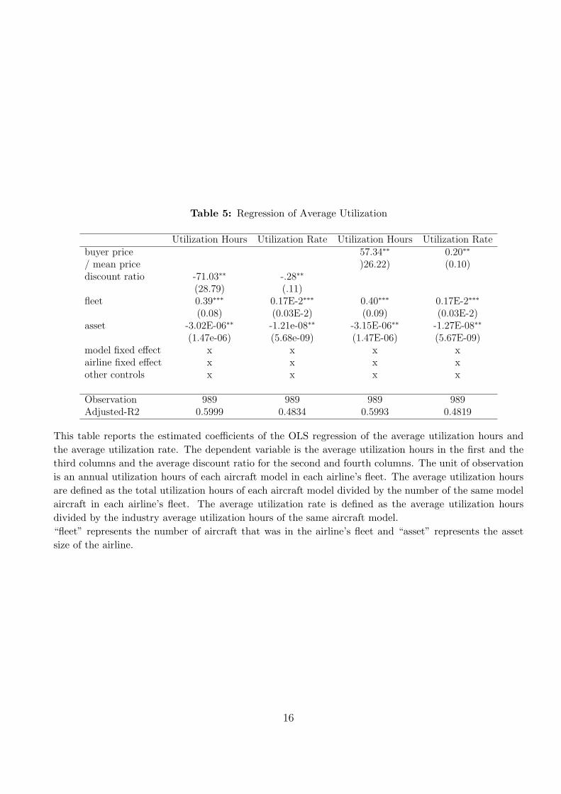
Table 5: Regression of Average Utilization

Utilization Hours Utilization Rate Utilization Hours Utilization Ratebuyer price 57.34∗∗ 0.20∗∗

/ mean price )26.22) (0.10)discount ratio -71.03∗∗ -.28∗∗

(28.79) (.11)fleet 0.39∗∗∗ 0.17E-2∗∗∗ 0.40∗∗∗ 0.17E-2∗∗∗

(0.08) (0.03E-2) (0.09) (0.03E-2)asset -3.02E-06∗∗ -1.21e-08∗∗ -3.15E-06∗∗ -1.27E-08∗∗

(1.47e-06) (5.68e-09) (1.47E-06) (5.67E-09)model fixed effect x x x xairline fixed effect x x x xother controls x x x x

Observation 989 989 989 989Adjusted-R2 0.5999 0.4834 0.5993 0.4819

This table reports the estimated coefficients of the OLS regression of the average utilization hours andthe average utilization rate. The dependent variable is the average utilization hours in the first and thethird columns and the average discount ratio for the second and fourth columns. The unit of observationis an annual utilization hours of each aircraft model in each airline’s fleet. The average utilization hoursare defined as the total utilization hours of each aircraft model divided by the number of the same modelaircraft in each airline’s fleet. The average utilization rate is defined as the average utilization hoursdivided by the industry average utilization hours of the same aircraft model.“fleet” represents the number of aircraft that was in the airline’s fleet and “asset” represents the assetsize of the airline.

16

price and quantity that actually happened rather than the complete menu of the price-quantity

relationship, the correlation can be always rationalized by a linear pricing strategy with transac-

tion specific slopes. However, it is a known fact that order quantities are an important factor to

get discounts when manufacturers and airlines negotiate over the price.9

Table 5 provide evidence that (III) the manufacturers price discrimination creates inefficiency

in aircraft allocation and transportation production. Ideally, to provide direct evidence of misallo-

cation, I need to present that there is dispersion in marginal productivity of aircraft across airlines.

However, marginal productivity of aircraft is difficult to measure. Instead, I use the utilization

rate as the indicator for marginal productivity, which is a standard proxy in the capital utilization

literature. For example, there is one-to-one correspondence between airlines’ productivity and

the utilization rate in Gavazza (2011).10 An important assumption behind is that the marginal

cost of utilization is increasing. When airlines decide the utilization rate, they equate marginal

cost of utilization to the marginal productivity. If the marginal cost of utilization is increasing,

a high utilization rate implies a high marginal cost and, therefore, high marginal productivity.

If we believe that the utilization rate is a good indicator for the marginal productivity, table 5

suggests that the manufacturers’ price discrimination creates inefficiency in aircraft allocation and

distorts production of transportation. From social planner’s point of view, more aircraft should be

allocated to airlines with high marginal productivity. However, the data suggest that airlines with

low utilization rate, therefore low marginal productivity, face lower price and have easier access

to the marginal aircraft, which creates misallocation of aircraft. The aircraft misallocation creates

welfare loss in airline market by creating inefficiency in production of transportation.

9The following articles in Bloomberg and the Economist are the examples that sup-port that the manufacturers price discriminate airlines and use a non-linear pricing strategy.http://www.bloomberg.com/news/2013-02-28/air-lease-expands-with-3-2-billion-order-for-boeing-777s.html,http://www.economist.com/blogs/gulliver/2013/06/easyjet .

10In Gavazza (2011), airlines derive per aircraft profit of π(u, θ) = θu− 0.5u2, where u is the utilization rate andθ is the productivity of the aircraft. Here, the optimal utilization rate u∗ = θ.

17

4 Model

The results in the previous section raise the following questions: Why is the misallocation sustained

in the equilibrium? How much is the welfare loss coming from the misallocation? To answer the

questions, I take a structural approach in the subsequent sections of the paper.

To start the analysis, I describe the model of the aircraft transactions and utilization in this section.

4.1 Theoretical Example

Before moving to the full model that I estimate structurally, I describe a simple theoretical example

to derive intuition for why there is allocative inefficiency and how we can restore the welfare loss by

potential policy interventions. To start with, I present a model of upstream firms and downstream

firms without any utilization part.

Upstream

Suppose two ex-ante identical firms, U1 and U2, sell a homogeneous intermediate good in two

periods. The marginal cost of production is constant within each period, but exhibits dynamic

economies of scale via a learning-by-doing effect. Let the marginal cost of production be

MCt(qit) = cu − kqit−1,

where qit−1 is the cumulative production amount of firm i up to period t− 1, and k captures the

degree of learning-by-doing.

Downstream

At each period, short-lived downstream firms arrive at the market. Downstream firms are heteroge-

neous in their demand of the intermediate good. Downstream firm derives utility from consuming

the good and has a utility function u(θ, q) = θq − 12q2 , where θ captures the heterogeneity of

downstream firms. The utility function induces a demand curve D(p, θ) = θ−p. Also assume that

the downstream firms live only one period.

Game Structure

The timing of the pricing and purchase decision is the following.

18

Period 1

1. Downstream firms arrive the market.

2. Upstream firms observe each downstream firm’s θ and simultaneously offer a (possibly

different) price to each downstream firm.

3. Each downstream firm decides how much to buy the good given the offered price and

receives utility from consumption minus the price she pays.

Period 2 The same structure repeats.

To simplify the analysis and to avoid complication coming from a tie, assume downstream firms

choose to buy from U1 if the same price is offered.

Proposition 1: There is an equilibrium with quantity discount in the first period.

Proof: In Appendix. ¥

The intuition behind the proposition is simple. The learning-by-doing effect creates ex-post market

power in the second period. If one upstream firm produce more in the first period, the firm

has lower marginal cost than its rival and earns profit by undercutting its rival’s marginal cost.

Given this ex-post market power, upstream firms compete in the first period to produce more.

Suppose that there are two downstream firms in the first period and also suppose the downstream

firms are heterogeneous in their demand for the intermediate good, the downstream firm with

larger demand is more attractive since serving the larger downstream firm increases production

more and determines which upstream firm will have the market power in the second period.

Therefore, competition between upstream firms lead to competition for the larger downstream

firm, which results in a quantity discount. Under the equilibrium with quantity discounts, the

smaller downstream pays more than the long-run marginal cost and the upstream firm earns long-

run profit. However, the long-run profit is extracted by the larger downstream firm as a result

of competition between upstream firms and she receive lower price than the smaller downstream

firm. The dispersion in the marginal price creates allocative inefficiency. Also, if the downstream

firms in the example use the good to produce final goods, then this example can also explain the

19

positive correlation between the price paid and utilization rate.11

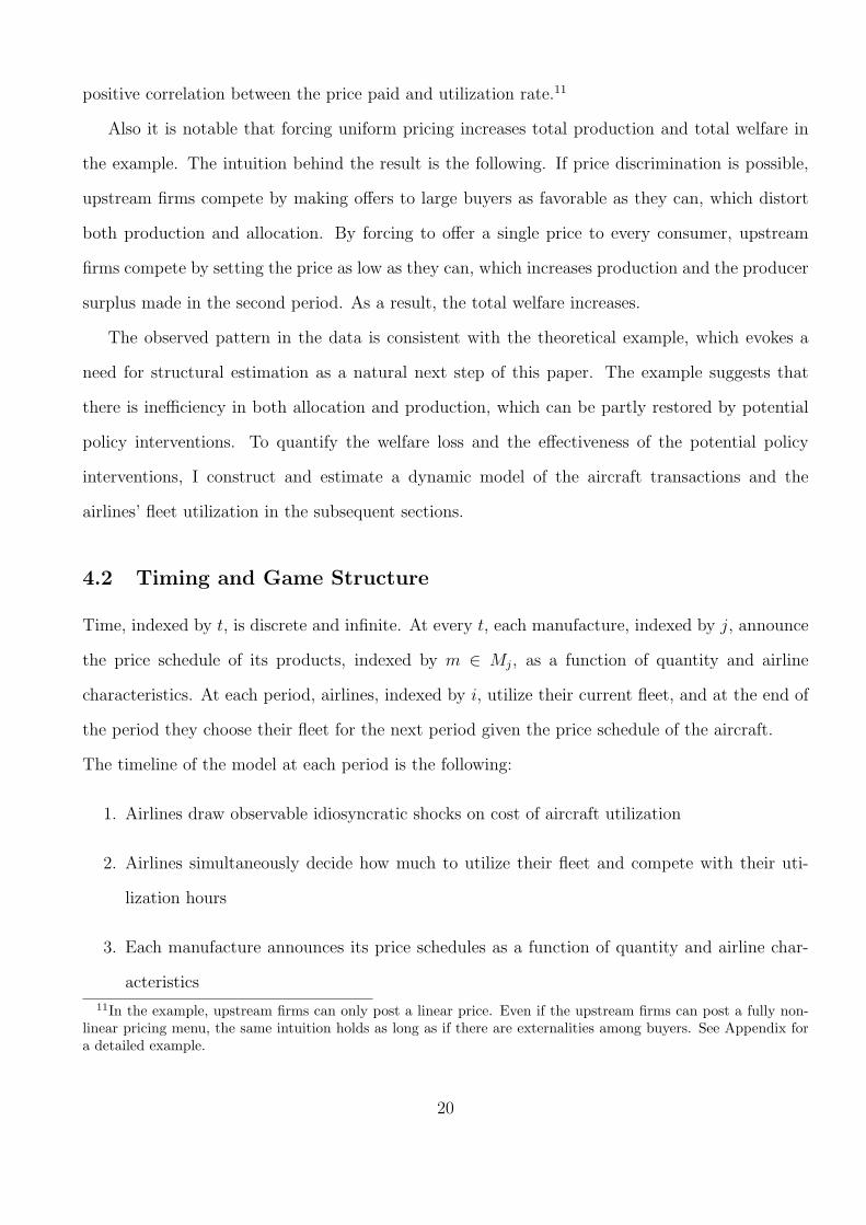
Also it is notable that forcing uniform pricing increases total production and total welfare in

the example. The intuition behind the result is the following. If price discrimination is possible,

upstream firms compete by making offers to large buyers as favorable as they can, which distort

both production and allocation. By forcing to offer a single price to every consumer, upstream

firms compete by setting the price as low as they can, which increases production and the producer

surplus made in the second period. As a result, the total welfare increases.

The observed pattern in the data is consistent with the theoretical example, which evokes a

need for structural estimation as a natural next step of this paper. The example suggests that

there is inefficiency in both allocation and production, which can be partly restored by potential

policy interventions. To quantify the welfare loss and the effectiveness of the potential policy

interventions, I construct and estimate a dynamic model of the aircraft transactions and the

airlines’ fleet utilization in the subsequent sections.

4.2 Timing and Game Structure

Time, indexed by t, is discrete and infinite. At every t, each manufacture, indexed by j, announce

the price schedule of its products, indexed by m ∈ Mj, as a function of quantity and airline

characteristics. At each period, airlines, indexed by i, utilize their current fleet, and at the end of

the period they choose their fleet for the next period given the price schedule of the aircraft.

The timeline of the model at each period is the following:

1. Airlines draw observable idiosyncratic shocks on cost of aircraft utilization

2. Airlines simultaneously decide how much to utilize their fleet and compete with their uti-

lization hours

3. Each manufacture announces its price schedules as a function of quantity and airline char-

acteristics

11In the example, upstream firms can only post a linear price. Even if the upstream firms can post a fully non-linear pricing menu, the same intuition holds as long as if there are externalities among buyers. See Appendix fora detailed example.

20

4. Airlines draw idiosyncratic shock on the cost of investment for each model and decide their

next period fleet

4.3 Period Payoff from Utilization

At the beginning of the period, each airline draws idiosyncratic shocks, εit = (ε1it, · · · , εM

it ), on

utilization cost of each model. The airline i’s cost of utilizing a model m aircraft for u hours is

cm(u, εmit ) = cm

0 + u (cm1 + cm

2 u + εmit ) ,

where cm1 + cm

2 u + εmit captures the marginal cost of utilization.

If airline i has fmit units of aircraft and if the average utilization hours of model m is u, then the

total cost of operation and total utilization hours are

fmit × cm(u, εm

it ) and fmit × u,

respectively. Also, at every t, airline i faces a residual demand function given the utilization

decision of all other airlines. Airline i faces the following inverse demand curve

P ti (Qi, Q−i) = dt + γi − δ1Qi − δ2

∑

j 6=i

Qj,

where Ql is airline l’s total utilization hours, dt is the time specific profitability of unit utilization

hour at period t and γi is the airline specific profitability of utilization.

The utilization decision of each airline is static and airlines compete by the utilization hours given

their fleet. Additional to the aircraft each airline owns, airlines can operates aircraft leased form

financial companies. Let rmt denote the rental cost of an aircraft at period t and lmit denote the

number of aircraft that airline i rents at period t. Here I assume the leasing market and the

used aircraft market is competitive and the rental price is determined exogenously. Then the best

21

response function of airline i given Q−i can be defined as

BRti(Q−it) = arg max

Qit,Lit

{(dt + γi − δ1Qit − δ2

∑

j 6=i

Qjt

)Qit

−M∑

m=1

(fm

it + lmit)cm(um

it , εmit )

−M∑

m=1

lmit rmt

}

s.t. Qit =M∑

m=1

(fm

it + lmit)um

it ,

where Lit = (l1it, · · · , lMit ) denotes a vector that counts i’s number of the rental choice of aircrafts.

Also, let Fit = (f 1it, · · · , fM

it ) denote the vector that represents airline i’s fleet in the subsequent

section in this paper.

Since airlines simultaneously decide their utilization hours, Nash equilibrium is characterized as

the fixed point of the best response function. The profit each airline derive at each period in

equilibrium is

πt(Q∗it, Q

∗−it, γi) =

(dt + γi − δ1Q

∗it − δ2

∑

j 6=i

Q∗jt

)Q∗

it

−M∑

m=1

(fm

it + lm∗it

)cm(um∗

it , εmit )−

M∑m=1

lm∗it rmt

s.t. Q∗it =

M∑m=1

(fm

it + lmit)um∗

it ,

where (Q∗it, L

∗it) = BRt

i(Q∗−it).

4.4 Investment Decision

Let πti(Ft) be the expected profit of airline i at period t in the equilibrium of the game de-

scribed above as a function of airlines’ fleet Ft = (F1t, · · · , FIt). Suppose airline i is expecting

the sequence of airlines’ fleet {F−it}∞t=s and the sequence of aircraft pricing menu {pt(q, γ) =(p1

t (q1, γ), · · · , pM

t (qt, γ))}∞t=s. Airline i maximizes the expected discounted sum of the future profit

22

defined as follows:

Vs(Fis, γi, {F−it}∞t=s, {pt(q, γ)}∞t=s) = max{Fit}∞t=sE

[∑∞t=s+1 β(t−s)

(πt

i(Ft)− pt−1

(qit, γi

)+ η′it

(qit

))]

subject to Fit+1 = δfitFit + qit,

(1)

where ηit = (η1it, · · · , ηM

it ) is a model specific idiosyncratic shock on the cost of investment and δfit

is the depreciation rate of aircraft. By the recursive structure, airline i’s investment strategy can

be characterized as a maximization problem of the following object. At each period, airline i’s

strategy given ps(·) is,

σ(Fis, γi, ηis,{F−it}∞t=s, {pt(q, γ)}∞t=s)

= maxFis+1

{−ps

(qis, Fis, γi

)+ η′is

(qis

)+ βVis+1(Fis+1, γi, {F−it}∞t=s, {pt(q, γ)}∞t=s)

}.

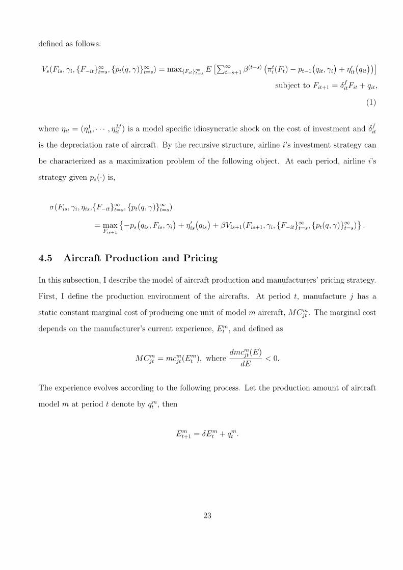
4.5 Aircraft Production and Pricing

In this subsection, I describe the model of aircraft production and manufacturers’ pricing strategy.

First, I define the production environment of the aircrafts. At period t, manufacture j has a

static constant marginal cost of producing one unit of model m aircraft, MCmjt . The marginal cost

depends on the manufacturer’s current experience, Emt , and defined as

MCmjt = mcm

jt(Emt ), where

dmcmjt(E)

dE< 0.

The experience evolves according to the following process. Let the production amount of aircraft

model m at period t denote by qmt , then

Emt+1 = δEm

t + qmt .

23

Note that the production experience exhibits “learning-and-forgetting”, which is a common phe-

nomenon in capital production.12 Under the production environment, the period profit of the

manufacture j can be described as follows. Let pmjt(·) denotes the price-quantity schedule of air-

craft model m and let qmit denotes airline i’s demand of aircraft model m at period t. Then the

manufacture j’s period profit at t, πpt

jt (Ejt, qt), is described as

πpt

jt (Et, qt) =∑

m∈Mj

(∑i∈I

pmjt(q

mit , γi)− qm

t mcmjt(E

mt )

),

where qmt =

∑i∈I qm

it .

Suppose manufacturer j is expecting the airlines’ investment strategy, σ, the sequence of air-

lines’ fleet, {Ft}∞t=s, and the sequence of aircraft pricing menu of its rival manufacturer, {p−jt(q, γ)}.Manufacturer j maximizes the expected discounted sum of the future profit defined as follows. Now,

let pjt(q, γ, Et, Ft) denote the price menu manufacture j propose given the state of manufacturers

and airlines. The value function of manufacturer j is defined as

Vjs(Es, σ, {Ft}∞t=s, {p−jt(q, γ)}) = max{pjt(·)}

E

[ ∞∑t=s

β(t−s)πpt

jt (Et, qt) | {pt(·)}]

, (2)

where qt and the evolution of state Et are induced from the investment strategy of airlines and

its rival’s pricing strategy. By the recursive structure, manufacturer j’s pricing strategy can be

characterized as a maximization problem of the following object. At each period, manufacturer

j’s strategy is,

pjs = σpj (Es,Fs, σ, {p−jt(q, γ)})

= maxp

{E

[πps

js (Es, qs) + βVjs(δEs + qs, σ, {Ft}∞t=s, {p−jt(q, γ)}) | p]} .

12Benkard (2000) provide empirical evidence of “learning-and-forgetting” in aircraft production. There are alsoa number of papers, including Levitt, List, and Syverson (2012) and Thompson (2007), that provide evidence ofthe phenomenon in different industries.

24

4.6 Solution Concept

To close the model, I use Oblivious Equilibrium as the solution concept in this paper. Oblivious

Equilibrium(OE) is a solution concept proposed by Weintraub, Benkard, and Roy (2008), in which

each firm is assumed to make decisions based only on its own state and knowledge of the long-

run average industry state, but not on the current information about competitors’ states. OE

is convenient in industries with many firms, and Weintraub, Benkard, and Roy (2008) provides

reasons to use OE as a close approximation to Markov Perfect Equilibrium (MPE).

In this paper, I make the following two assumptions.

Assumption 1. Airlines play Oblivious strategy. When airline i makes its investment decision,

it bases its decision only on its own fleet, current proposed pricing menu and the long-run average

industry state. In particular, when airline i takes expectation of expression (1), it takes expectation

given the sequence of airlines’ fleet {F−it = F ∗−i}∞t=s and the sequence of aircraft pricing menu

{pt(·) = p∗(·)}∞t=s, where F ∗−i and p∗(·) is the long-run average fleet of airlines and the pricing

menu of manufacturers.

Assumption 2. Manufacturers play Oblivious strategy, where they are oblivious of airlines’ actual

fleet. When manufacturer j decides the pricing menu of its product, it bases its decision only on

its own state, other manufacturers’ states and the long-run average industry state of airlines. In

particular, when manufacturer j takes expectation of expression (2), it takes expectation given the

sequence of airlines’ fleet {Ft = F ∗}∞t=s.

The most related paper to these assumptions is Benkard, Jeziorski, and Weintraub (2013),

where the authors develop an application of OE to to concentrated industries. In the paper, the

authors define an extended notion of oblivious equilibrium, Partially Oblivious Equilibrium (POE),

in which the state of a subset of players enter into the players’ strategies. Since players ignore the

actual state of all other players in OE, POE is a generalization of OE in the sense that the players

take the actual state of some of the players into account. Since there are more than thirty airlines

in the data, the dimension of the state variables is too large to solve the model using Markov

Perfect Equilibrium. Adopting OE (POE) makes the model tractable and feasible to estimate.

25

Also, since there are a large number of airlines, assuming players are oblivious of the actual state

of airlines may work as a good approximation of MPE.

5 Estimation and Identification

In the estimation, I take three steps to estimate the whole model. First, I estimate the parameters

on the utilization model and the airline specific profitability. The utilization model is a completely

static model and it can be estimated from the static optimality of the observed utilization decision

separately from all the remaining model. Using the estimates, I next estimate the value function

of the airlines where I heavily take advantage of the oblivious assumptions. By substituting

the estimated airline specific profitability and putting distributional assumptions on the cost of

investment, I estimate the value function nonparametrically. Finally, I estimate the parameters on

the production model. With the estimated value function of airlines, I can estimate the outcome of

the transaction between manufacturers and airlines for any arbitrary pricing menus. The optimality

of the observed pricing menus induces a set of inequalities, which identifies the parameter. In this

section, I describe the estimation and identification step by step.

To simplify the notation, {F ∗i } and {p∗(q, γ)} are not explicitly written when I write down the

value function.

5.1 Utilization Model

I specify the inverse demand curve as follows. Since major airlines and regional airlines shows

different patterns in the utilization, I allow the parameter to take different values between these

two types of airlines.

The inverse demand function takes the following form if airline i is a major airline

P ti (Qi, Q−i) = dt + γi − δmajorQi −

∑

j 6=i,j∈major

δmajormajorQj −

∑

j 6=i,j∈regional

δregionalmajor Qj,

26

and if airline i is a regional airline

P ti (Qi, Q−i) = dt + γi − δregionalQi −

∑

j 6=i,j∈major

δmajorregionalQj −

∑

j 6=i,j∈regional

δregionalregionalQj,

where γ captures the airline specific profitability of utilization and dt captures the time specific

demand sifter. Also, I specify the cost of utilization as

cm(u, εmit ) = c0 + u (cm

1 + κcm1 u + εm

it ) .

where κ captures the increasing marginal cost of utilization and εmit is independent across time,

model and airlines.

Assumption 3 (Distributional of the Shock on the Utilization Cost). εs are distributed identically

and independently as N(0, σ2ε ).

Assumption 4 (Distribution of the Demand State). dts are distributed identically and indepen-

dently as N(d, σ2d).

The parameter to be estimated is d = (d1, · · · , dT ), γ = (γ1, · · · , γI), δ, c0, c1 = (c11, · · · , cM

1 ),

κ and σ2ε . The data contains annual utilization hours, cm

it and the leasing decision of airlines, lmit .

One important missing information is the rental cost aircraft, which I estimate using the data on

the transaction price of used aircraft.

Assumption 5 (Leasing Market). The aircraft leasing market and secondary market are compet-

itive and the rental price of aircraft is distributed as N(r, σ2r) at each year.

This assumption allows me to estimate the rental cost of aircraft. In the data, I observe the

transaction price of aircraft, which is informative about the cost of holding an aircraft for one year.

Suppose a leasing company buy an aircraft at year t and sell it at t+1, the difference in the aircraft

price at t and t + 1 is the rental cost of the aircraft under the assumption of competitiveness. In

the subsequent analysis, I substitute the estimated rental price in the estimation of the utilization

27

model parameter.13 The parameter is identified from the variation in the utilization rate and the

variation in rental choice. For a fixed fleet, airlines equate the marginal cost and the marginal

revenue of utilization. The variation in the utilization rate identifies the relative value of the

parameter of utilization cost and profitability. For example, the relative value of dt and γis are

identified from the relative level of utilization rate across airlines and time. Conditional on the fleet,

the variation in utilization rate across airlines identifies the relative level of γi, and the variation

in overall utilization level across year identifies that of dt. The rental choice identifies the absolute

level of the parameter.

The optimal utilization hours of airline i satisfies

∂P ti (Qit, Q−it)− Ci(Qit)

∂umit

= 0

⇔ P ti (Qt)− δiu

mit − (cm

1 + 2κcm1 u + εm

it ) = 0 ∀m.

This equality conditions translate into a set of moment equality, which is

E

[(dt − γi − δ1Qit − δ2

∑−i

Q−it

)− δ1umit −

(cm1 + 2κcm

1 umit

)]

= 0 ∀m, i, t.

The absolute value of the parameter and c0 is identified from the optimality of the rental choice.

The cost increasing (benefit of decreasing) the observed rental choice can not be larger than the

decrease (increase) in the per unit utilization cost, which identifies the fixed cost, c0, and the

absolute value of the parameter. The rental decision of airline i satisfies the optimality condition

13In the estimation of the rental price, I first estimate the used aircraft price nonparametrically for each model,m, and year, t. I specify the estimation equation as

pmlt = pm

t (agelt) + εmlt ,

where l is a index for transactions, pmlt is the observed transaction price of model m aircraft that is agelt year old

and εmlt is meant to capture measurement error. Gavazza (2011) notes that the actual transaction price is explained

well by the list price, which is calculated by the age of the model. The rental price is estimated by

rmt = pm

t (agelt)− βpmt+1(agelt + 1),

where agelt is the average age of the model m used aircraft traded at time t and β is the discount factor. Here Iset the discount factor to be 0.95.

28

as follows.

maxQit,Lit

(dit − δiQit −

∑

j 6=i

δjQjt

)Qit

−M∑

m=1

(fm

it + lmit)cm(um

it , εmit )−

M∑m=1

lmit rmt

≥ maxQit,Lit 6=L∗it

(dit − δiQit −

∑

j 6=i

δjQjt

)Qit

−M∑

m=1

(fm

it + lmit)cm(um

it , εmit )−

M∑m=1

lmit rmt

This inequality conditions translate into a set of moment inequality conditions for the parameters.

I estimate the parameter by minimizing the objective function which has both the above equality

and inequality conditions.

5.2 Investment Decision

First, I specify the distribution of the shocks on investment cost.

Assumption 6 (Distributional Assumption on the Error). ηs are distributed identically and in-

dependently as N(0, σ2η).

At each period, airline i maximizes the value function given the proposed price menus and the

period shock on investment cost. In the maximization problem, {ps

(qis, γi

)} can be backed out

from the data. Therefor the only dynamic part to be estimated is the value function. With the

distributional assumption on η, the optimality of the airlines’ fleet choice induces the likelihood of

the data.

I take two steps in the estimation of the value function. In the first step, I estimate the manu-

facturers’ pricing menus nonparametrically. In the second step, I substitute the estimated pricing

menus in the likelihood function and estimate the value function nonparametrically by sieve MLE.

From the optimality of the airline i’s investment decision,

qis = σ(Fis, γi) = arg maxq

{−ps

(q, γi

)+ η′is

(q)

+ Vis+1(q + Fis, γi)}

.

29

If the price menu is observed, the condition above translates into conditions on the range of ηis.

From the optimality condition, changing qis to qis + 1 or qis − 1 gives,

− (ps

(qis, γi

)− ps

(qis + 1, γi

))+ (Vis+1(qis + Fis, γi)− Vis+1(qis + 1 + Fis, γi)) ≥ ηis

− (ps

(qis, γi

)− ps

(qis − 1, γi

))+ (Vis+1(qis + Fis, γi)− Vis+1(qis − 1 + Fis, γi)) ≥ −ηis.

Therefore, the probability of observing qis in the data is equal to

Pr(− (

ps

(qis, γi

)− ps

(qis + 1, γi

))+ (Vis+1(qis + Fis, γi)− Vis+1(qis + 1 + Fis, γi))

≥ ηis ≥(ps

(qis, γi

)− ps

(qis − 1, γi

))− (Vis+1(qis + Fis, γi)− Vis+1(qis − 1 + Fis, γi))). (3)

By approximating the value function by a sieve function, I can estimate the parameter on the sieve

function by MLE. However, this approach is not feasible because the price menu is not observed

and, therefore, a two step approach is needed.

In the data, I observe (pmit , q

mit , γi) for each aircraft order, which allows me to estimate the price menu

nonparametrically. In the first step, I estimate the pricing menu using the following specification.

For each t,

pmit = pm

t

(qmit , γi

)+ emit,

where emit is independent with qmit and γi.

14 Here emit is meant to capture measurement error in

the data. By approximating pmt by a sieve function and substituting γi for γi, the price menu can

be estimated by a standard nonparametric regression method.

In the second step, I substitute pmit and γi for pm

it and γi in the expression (3), which induces the

14Under the model, the price menu is a function of the state and it should be estimated as a function of the staterather than than an independent function for each t. However, the state of manufacturers is not observed sincethe depreciation rate of the experience, δ, is unknown and it is infeasible to estimate it as a function of the state.One alternative estimation strategy is to jointly estimate the production side parameter, but it is computationallydemanding. In order to estimate the airlines’ value function, a consistent estimator of the price menu for each t issufficient.

30

likelihood of the data as

Pr(− (

ps

(qis, γi

)− ps

(qis + 1, γi

))+ (Vis+1(qis + Fis, γi)− Vis+1(qis + 1 + Fis, γi))

≥ ηis ≥(ps

(qis, γi

)− ps

(qis − 1, γi

))− (Vis+1(qis + Fis, γi)− Vis+1(qis − 1 + Fis, γi))). (4)

As long as ps and γi are consistent for pmit and γi, the probability in expression (3) and (4) are

asymptotically equivalent. Therefore, sieve MLE in which I maximize the likelihood in expression

(4) gives a consistent estimator for the airline’s value function. 15

5.3 Aircraft Production

In this subsection, I describe the estimation of the aircraft production parameter. First, I specify

the production technology as follows.

MCmjt = mcm + ζ

((Em

t )−ρ), Em

t+1 = δEmt + qm

t ,

where ζ, ρ and δ is the parameter to be estimated.

The estimation relies on simulations similar to Bajari, Benkard, and Levin (2007). Let Vj(Et, σp)

denote the expected discounted sum of the future profit of manufacturer j when manufacturers play

strategy σp. The optimality of the observed pricing menu gives the following inequality conditions.

Vj(Et, σp∗) ≥ Vj(Et, σ

pj , σ

p∗−j) ∀σp

j , j . (5)

Given the estimated value function of airlines, I can simulate the transaction outcome for arbitrary

pricing menus. Therefore, I can simulate both left and right hand side of the inequality, which

construct a set of inequality conditions. I assume that the production parameter is identified by

the inequality conditions and the parameter can be estimated similar to the method proposed by

Bajari, Benkard, and Levin (2007). A notable difference from Bajari, Benkard, and Levin (2007)

comes from the fact that the exact state is not observed in my model. Even though I see the

15In the estimation, I approximate the objective by a polynomial function of its argument.

31

complete history of the aircraft production history, the exact state is a function of the depreciation

rate of the experience, δ, and the production history. When I simulate Vj(Et, σp∗; θm) for a fixed

parameter value θm, I first calculate Et(δ). Given the value of Et(δ), I next estimate the observed

price menu as a nonparametric function of Et(δ), quantity and γi. After I estimate the value

function of airlines and observed pricing strategy, I can simulate the sequence of market outcome

for arbitrary length, which gives the value of Vj(Et, σp∗; θm) by taking the average of many different

sequence of market outcome. Similarly, by creating an alternative pricing strategy, I can simulate

the value of Vj(Et, σpj , σ

p∗−j). I estimate the parameter using the inequality (5). To be precise, the

estimator, θ, is

θ = arg min∑

j

∑

alt

(min

{Vj(Et, σ

p∗)− Vj(Et, σp,altj , σp∗

−j), 0})2

.

6 Result and Counterfactual

In this section, I present the estimation and counterfactual result. Table 6 shows the main esti-

mates of the parameter. κ captures the increasing part of the marginal cost of utilization. Since the

marginal cost of utilization is increasing, the dispersion in the utilization rate implies the welfare

loss. For any fixed amount of total utilization hours, the total utilization cost is minimized when

the utilization rate is equalized among airlines. In the aircraft production, ζ captures the produc-

tion cost that goes to 0 as the manufacturers’ experience goes to infinity. The learning-by-doing

accounts for up to about 30% of the total cost of production. Compared to the existing literature,

the estimates are in a reasonable range. Benkard (2000) reports the forgetting rate to be about

61% and the effect of the cost reduction to be about 40%. 16

In the counterfactual analysis, I compare the equilibrium market outcome and welfare under

two alternative market designs: the manufacturers post a single uniform price to all airlines for

each of their products (Uniform Pricing); the manufacturers post one price-quantity menu to all

airlines for each of their products (Grand Menu Pricing). The first counterfactual analysis is

16Levitt, List, and Syverson (2012) and Thompson (2007) report much higher depriciation rate. They report theestimates for δ (compounded for annual rate) to be about 20% to 50%.

32

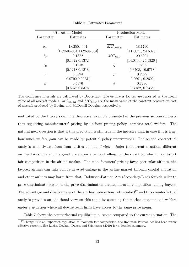
Table 6: Estimated Parameters

Utilization Model Production ModelParameter Estimates Parameter Estimates

δm 1.6250e-004 MCboeing 18.1790[1.6250e-004,1.6250e-004] [ 11.8071, 24.5026 ]

δr 0.1372 MCMcD 20.6391[0.1372,0.1372] [14.0366, 25.5326 ]

c0 0.1218 ζ 7.5892[0.1218,0.1218] [6.3708, 10.6718]

c1 0.0894 ρ 0.2692[0.0790,0.0923 ] [0.2691, 0.2692]

κ 0.5376 δ 0.7296[0.5376,0.5376] [0.7182, 0.7368]

The confidence intervals are calculated by Bootstrap. The estimates for c1s are reported as the meanvalue of all aircraft models. MCboeing and MCMcD are the mean value of the constant production costof aircraft produced by Boeing and McDonell Douglas, respectively.

motivated by the theory side. The theoretical example presented in the previous section suggests

that regulating manufacturers’ pricing by uniform pricing policy increases total welfare. The

natural next question is that if this prediction is still true in the industry and, in case if it is true,

how much welfare gain can be made by potential policy interventions. The second contractual

analysis is motivated from from antitrust point of view. Under the current situation, different

airlines faces different marginal price even after controlling for the quantity, which may distort

fair competition in the airline market. The manufacturers’ pricing favor particular airlines, the

favored airlines can take competitive advantage in the airline market through capital allocation

and other airlines may harm from that. Robinson-Patman Act (Secondary-Line) forbids seller to

price discriminate buyers if the price discrimination creates harm in competition among buyers.

The advantage and disadvantage of the act has been extensively studied17 and this counterfactual

analysis provides an additional view on this topic by assessing the market outcome and welfare

under a situation where all downstream firms have access to the same price menu.

Table 7 shows the counterfactual equilibrium outcome compared to the current situation. The

17Though it is an important regulation to maintain fair competition, the Robinson-Patman act has been rarelyeffective recently. See Luchs, Geylani, Dukes, and Srinivasan (2010) for a detailed summary.

33

Table 7: Counterfactual Outcome

Uniform PricingBoeing McDonnell Douglas Total Airlines

Average Price Change −9.46% −5.59% −8.45% –Average production Change 12.34% 6.02% 10.59% –Utilization Rate – – – −9.32%Total Utilization Hours – – – 0.28%

Grand Menu Pricing

Average Price Change −6.54% −12.56% −8.28% –Average production Change 8.32% 14.71% 10.01% –Utilization Rate – – – −7.44%Total Utilization Hours – – – 1.89%

first half of the table shows the counterfactual outcome under the uniform pricing regulation. By

forcing uniform pricing, the average price of aircraft decreases and the production amount increases

for both Boeing and McDonnell Douglas. The increase in aircraft production results in more total

utilization hours and lower utilization rates. Since the marginal cost of utilization is increasing

and the average aircraft price has decreased, airlines buy more aircraft and decrease the utilization

rate, which ends up in lower the utilization rate. Similar patterns are reported in the second half

of the table 7. The second half reports the equilibrium outcome under the grand menu pricing

regulation. Under the grand menu pricing, manufacturers can still sort airlines by proposing

non-linear pricing menu, but manufacturers need to offer the same menu to all airlines. Since

the menu can be non-linear, the pricing can creates dispersion in the marginal price. However,

allowing a non-linear pricing has, at least, two advantages over uniform pricing. Under uniform

pricing regulation, both upstream firms and downstream firms suffer from double-marginalization,

which may be mitigated by allowing non-linear pricing. Also, non-linear pricing helps upstream

firms to screen downstream firms in the dimension of unobserved demand size. It is theoretically

known that, under the existence of asymmetric information in buyers’ demand, allowing sellers to

design non-linear pricing to screen the buyers helps to increase production. These two positive

effect on aircraft production offset the inefficiency coming from dispersion in marginal price. The

34

important take away from table 7 is that both counterfactual results suggest that the main source

of inefficiency is manufacturers’ price discriminatin across airlines and shutting down the channel

of such price discrimination can help to restore efficiency.

Table 8: Counterfactual Welfare

Uniform PricingBoeing McDonnell Douglas Airlines Consumer Total

Welfare Change (in % ) 0.14% −0.89% 10.61% 0.38% 1.62%Welfare Change (in $ 1M) 20 −9 489 58 557

Grand Menu Pricing

Welfare Change (in % ) 0.14% −0.10% 10.88% 4.18% 3.33%Welfare Change (in $ 1M) 19 −2 501 626 1144

Table 8 shows the counterfactual welfare change under uniform pricing and grand menu pricing.

In both cases, manufacturers faces higher competition intensity and decreases their price on aver-

age. However, the manufacturers’ profit is almost unchanged. Higher competition intensity leads

to lower revenue per unit sales but, at the same time, it increases total production and leads to

lower unit costs via the learning-by-doing effect. In terms of welfare, higher competition intensity

leads the price closer to the long-run marginal cost of production, which helps to restore efficiency.

As in the previous table, the counterfactual results are similar in both uniform pricing and grand

menu pricing cases, which again suggests ensuring a fair competition environment is important to

help the market mechanism to work well.

7 Conclusion

In this paper, I present evidence that suggests capital misallocation in aircraft and airline industries.

I present a simple theoretical example to show that the learning-by-doing effect in production

and competition among upstream firms lead to aircraft price discrimination. The existence of

economies of scale in production creates a incentive to treat large buyers better, which distorts

both production and allocation of aircraft in favor of large buyers. I further construct and estimate

35

a dynamic structural model of the industries. The model captures economies of scale in aircraft

production via a learning-by-doing effect and both second and third degree price discrimination

in aircraft market. Using the estimated parameter, I simulate the equilibrium outcome under

alternative pricing regulations. The result suggests that manufacturers’ ability to price discriminate

airlines results in lower production of aircraft and lower total welfare. Forcing manufacturers to

treat all airlines equally does not only ensures fair competition in the airline industry but also

increases efficiency in both aircraft and airline industries.

36

References

Armstrong, M., and J. Vickers (2010): “Competitive Non-linear Pricing and Bundling,”

Review of Economic Studies, 77 (1)30-60, pp. 30–60.

Bajari, P., C. L. Benkard, and J. Levin (2007): “Estimating Dynamic Models of Imperfect

Competition,” Econometrica, 75(5), pp. 1331–1370.

Benkard, C. L. (2000): “Learning and forgetting: The dynamics of aircraft production,” Amer-

ican Economic Review, 90(4), pp. 1034–1054.

(2004): “A Dynamic Analysis of the Market for Wide-Bodied Commercial Aircraft,”

Review of Economic Studies, 71 (3), pp. 581–611.

Benkard, C. L., P. Jeziorski, and G. Y. Weintraub (2013): “Oblivious Equilibrium for

Concentrated Industries,” mimeo.

Besanko, D., U. Dorazelski, Y. Kryukov, and M. Satterthwaite (2010): “Learningby-

Doing, Organizational Forgetting, and Industry Dynamics,” Econometrica, 78 (2), pp. 453–508.

Busse, M., and M. Rysman (2005): “Competition and Price Discrimination in Yellow Pages

Advertising,” RAND Journal of Economics, 37, 378–390.

Cabral, L. M. B., and M. H. Riordan (1994): “The Learning Curve, Market Dominance,

and Predatory Pricing,” RAND Journal of Economics, 62(5), pp. 1115–1140.

Chipty, T., and C. M. Snyder (1999): “The role of firm size in bilateral bargaining: A study

of the cable television industry,” Review of Economics and Statistics, 81(2), pp. 326340.

Ellison, S. F., and C. Snyder (2010): “Countervailing Power in Wholesale Pharmaceuticals,”

Journal of Industrial Economics, 58(1, pp. 32–53.

Ericson, R., and A. Pakes (1995): “Markov-Perfect Industry Dynamics: A Framework for

Empirical Work,” Review of Economic Studies, 62(1), 53–82.

37

Foster, L., J. C. Haltiwanger, and C. Syverson (2008): “Reallocation, Firm Turnover,

and Efficiency: Selection on Productivity or Profitability?,” American Economic Review, 98(1),

394–425.

Fudenberg, D., and J. Tirole (1983): “Learning-by-Doing and Market Performance,” The

Bell Journal of Economics, 14(2), 522–530.

Gans, J. S., and S. P. King (2002): “Exclusionary contracts and competition for large buyers,”

International Journal of Industrial Organization, 20(9), 13631381.

Gavazza, A. (2011): “The Role of Trading Frictions in Real Asset Markets,” American Economic

Review, 101(4), 1106–43.

Hsieh, C.-T., and P. J. Klenow (2009): “Misallocation and Manufacturing TFP in China and

India,” The Quarterly Journal of Economics, 124(4), 1403–1448.

Kalouptsidi, M. (2010): “Time to Build and Shipping Prices,” Working Paper.

Levitt, S. D., J. A. List, and C. Syverson (2012): “Toward an Understanding of Learning

by Doing: Evidence from an Automobile Assembly Plant,” mimeo.

Luchs, R., T. Geylani, A. Dukes, and K. Srinivasan (2010): “The End of the Robinson-

Patman Act? Evidence from Legal Case Data,” Management Science, 56, 2123–2133.

Mortimer, J. H. (2008): “Vertical Contracts in the Video Rental Industry,” Review of Economic

Studies, 75(1), 165–199.

Ohashi, H. (2005): “Learning by doing, export subsidies, and industry growth: Japanese steel in

the 1950s and 1960s,” Journal of International Economics, 66(2), 297–323.

Pakes, A., M. Ostrovsky, and S. Berry (2007): “Simple estimators for the parameters of

discrete dynamic games (with entry/exit examples),” The RAND Journal of Economics, 38(2),

pp. 373399.

Restuccia, D., and R. Rogerson (2008): “Policy distortions and aggregate productivity with

heterogeneous establishments,” Review of Economic Dynamics, 11(4), 707720.

38

Rochet, J.-C., and L. A. Stole (2002): “Nonlinear Pricing with Random Participation,”

Review of Economic Studies, 69 (1), 277–311.

Snyder, C. M. (1996): “A Dynamic Theory of Countervailing Power,” The RAND Journal of

Economics, 27(4), pp. 747–769.

Sorensen, A. T. (2003): “Insurer-hospital bargaining: negotiated discounts in post-deregulation

connecticut,” The Journal of Industrial Economics, 51(4), pp. 469–490.

Spence, A. M. (1981): “The Learning Curve and Competition,” The Bell Journal of Economics,

12(1), pp. 49–70.

Stole, L. A. (1995): “Nonlinear Pricing and Oligopoly,” Journal of Economics & Management

Strategy, 4(4), 529562.

Thompson, P. (2007): “How much did the liberty shipbuilders forget?,” Management Science,

53(6), pp. 908918.

Thornton, R. A., and P. Thompson (2001): “Learning from Experience and Learning from

Others: An Exploration of Learning and Spillovers in Wartime Shipbuilding,” The American

Economic Review, 91(5), pp. 1350–1368.

Villas-Boas, S. B. (2002): “Vertical Relationships between Manufacturers and Retailers: In-

ference with Limited Data,” Review of Economic Studies, 74, pp. 625652.

Weintraub, G. Y., C. L. Benkard, and B. V. Roy (2008): “Markov Perfect Industry

Dynamics With Many Firms,” Econometrica, 76(6), 1375141.

Wright, T. P. (1936): “Factors affecting the cost of airplanes,” Journal of the Aeronautical

Sciences, 3(4), 122–128.

39

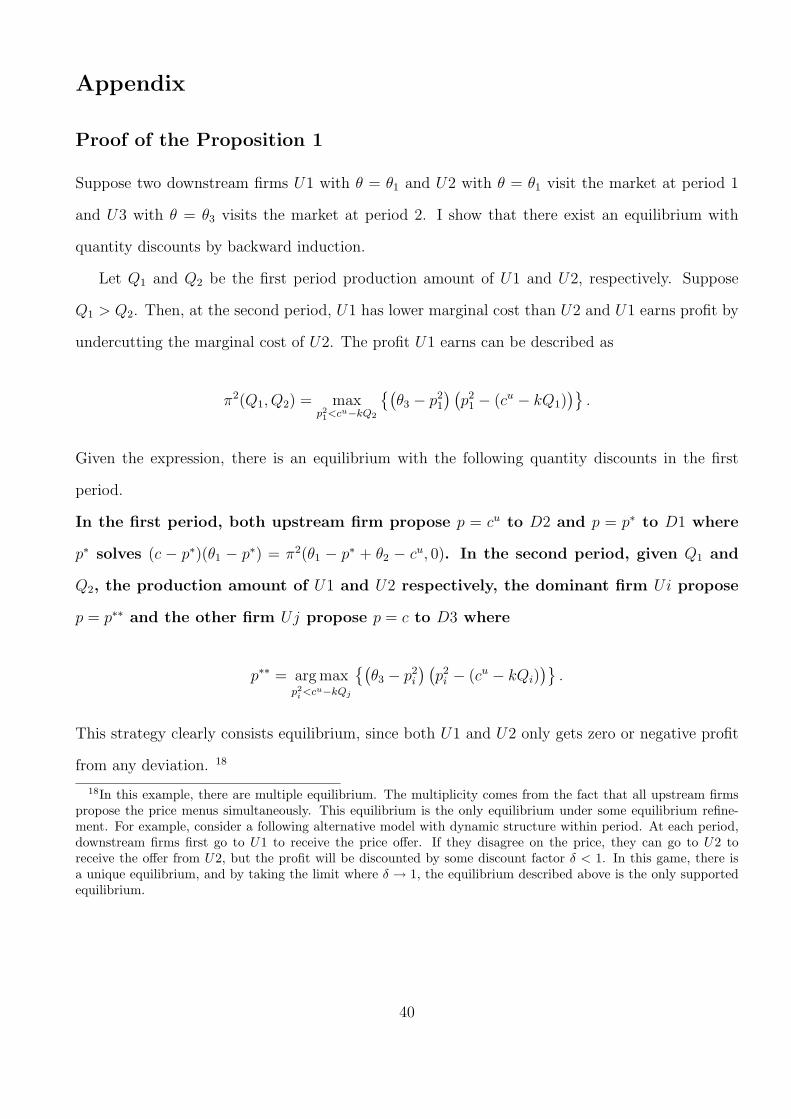
Appendix

Proof of the Proposition 1

Suppose two downstream firms U1 with θ = θ1 and U2 with θ = θ1 visit the market at period 1

and U3 with θ = θ3 visits the market at period 2. I show that there exist an equilibrium with

quantity discounts by backward induction.

Let Q1 and Q2 be the first period production amount of U1 and U2, respectively. Suppose

Q1 > Q2. Then, at the second period, U1 has lower marginal cost than U2 and U1 earns profit by

undercutting the marginal cost of U2. The profit U1 earns can be described as

π2(Q1, Q2) = maxp21<cu−kQ2

{(θ3 − p2

1

) (p2

1 − (cu − kQ1))}

.

Given the expression, there is an equilibrium with the following quantity discounts in the first

period.

In the first period, both upstream firm propose p = cu to D2 and p = p∗ to D1 where

p∗ solves (c − p∗)(θ1 − p∗) = π2(θ1 − p∗ + θ2 − cu, 0). In the second period, given Q1 and

Q2, the production amount of U1 and U2 respectively, the dominant firm Ui propose

p = p∗∗ and the other firm Uj propose p = c to D3 where

p∗∗ = arg maxp2

i <cu−kQj

{(θ3 − p2

i

) (p2

i − (cu − kQi))}

.

This strategy clearly consists equilibrium, since both U1 and U2 only gets zero or negative profit

from any deviation. 18

18In this example, there are multiple equilibrium. The multiplicity comes from the fact that all upstream firmspropose the price menus simultaneously. This equilibrium is the only equilibrium under some equilibrium refine-ment. For example, consider a following alternative model with dynamic structure within period. At each period,downstream firms first go to U1 to receive the price offer. If they disagree on the price, they can go to U2 toreceive the offer from U2, but the profit will be discounted by some discount factor δ < 1. In this game, there isa unique equilibrium, and by taking the limit where δ → 1, the equilibrium described above is the only supportedequilibrium.

40

Comparison with Uniform Pricing

Now consider a policy intervention which force the upstream firms to post a uniform price to all

downstream firms in the previous example. Then, the following consists an equilibrium.

In the first period, both upstream firm propose p = p∗u to all downstream firms where

p∗u solves (c − p∗u)(θ1 + θ2 − p∗u) = π2(θ1 + θ2 − p∗u, 0). In the second period, given Q1 and

Q2, the production amount of U1 and U2 respectively, the dominant firm Ui propose

p = p∗∗u and the other firm Uj propose p = c to D3 where

p∗∗u = arg maxp2

i <cu−kQj

{(θ3 − p2

i

) (p2

i − (cu − kQi))}

.

Note that p∗ > p∗u and p∗∗ > p∗∗u . It shows that with uniform pricing regulation, the production

increases in both the first and second period and increases total welfare.

Examples of Positive Relationship Between Price and Utilization Rate

Suppose two ex-ante identical upstream firms sell homogeneous intermediate good in two periods.

The marginal cost of production is constant within period, but exhibits dynamic economy of scale

by the learning-by-doing effect. In the example, assume the marginal cost of production is

MCi(qt−1) = c− kqt−1,

where qt−1 is the cumulative production amount up to period t− 1, and k captures the degree of

learning-by-doing.

Also, suppose at each period two downstream firms arrive. Each downstream firm operates in a

monopoly market and faces a final good demand curve of D(p, θ) = θ − p, where θ captures the

heterogeneity of each downstream firm’s profitability. To produce the final good, downstream firms

utilize the intermediated good. Let q be the amount of intermediate good and u be the utilization

41

rate. Suppose the production function and cost function are given as follow:

out put = qu

cost = q(u + au2),

where a captures the increasingly marginal cost of utilization. Each downstream firm first purchases

the intermediate good and then decides how much to utilize it.

Now consider a Bertrand game where upstream firms choose price in the intermediate good market

and downstream firms choose the price and utilization rate. Suppose downstream firms with θ = θ1

and θ = θ2 > θ1 arrive at period 1 and both downstream firms are with θ = θ3 at period 2 .

To abstract away the screening aspect, suppose upstream firms can offer different price for each

downstream firms.19 There is a subgame perfect equilibrium where the downstream firm with

θ = θ2 receives more favorable offer. The intuition behind the result is the same as the previous

example.

Given the game structure, first solve for the downstream firm given θ and amount of inter-

mediate good q. The profit that the downstream firm gets can be expressed as a function of the

utilization rate,

π(u, q, θ) = (θ − uq)uq − q(u + au2).

The optimal utilization rate will be

u∗ =(θ − 1)

2(q + a),

and the optimal monopoly profit is

π∗(q, θ) =(θ − 1)2q

4(q + a).

This monopoly profit induces a demand function in the intermediate goods market. The demand

19Also, to avoid complication coming from ties, assume if the offered prices are the same, all downstream firmsprefer buying the good from firm 1.

42

function of type θ downstream firm is simply the derivative of π∗ and

D(q, θ) =∂

∂qπ∗(q, θ) =

(θ − 1)2a

4(q + a)2.

Now, I can solve for the subgame perfect equilibrium.

First, note that in period 2, if one of the upstream firm has advantage in the production cost, he

charges all the downstream firms a price equals to the marginal cost of the other upstream firm.

Let the profit of firm i in the period 2 given the period 1 production denote by πu2i(q

1i , q

1j ).

Now consider the period 1 incentive. In equilibrium, firm 2 offer p1 = c to θ = θ1, but price, p2,

strictly less than c to θ = θ2. Here the reason for the pricing to be an equilibrium is the same as

in the previous example.

Next, consider the relationship between the offered price and the utilization rate. Downstream

firms equate the offered price and the marginal profit, which gives

p = D(q, θ).

By solving for u∗,

u∗ =

√p

a.

This equation implies that there is a one-to-one correspondence and a positive relationship between

the price offered and utilization rate. The intuition is simple. When downstream firms make their

production decision, they take two factor prices into account; the price of capital and the cost of

utilization. If a downstream firm is offered a lower price of capital, the relative price of capital

become lower and, therefore, buys more capital and decreases the utilization rate.

43

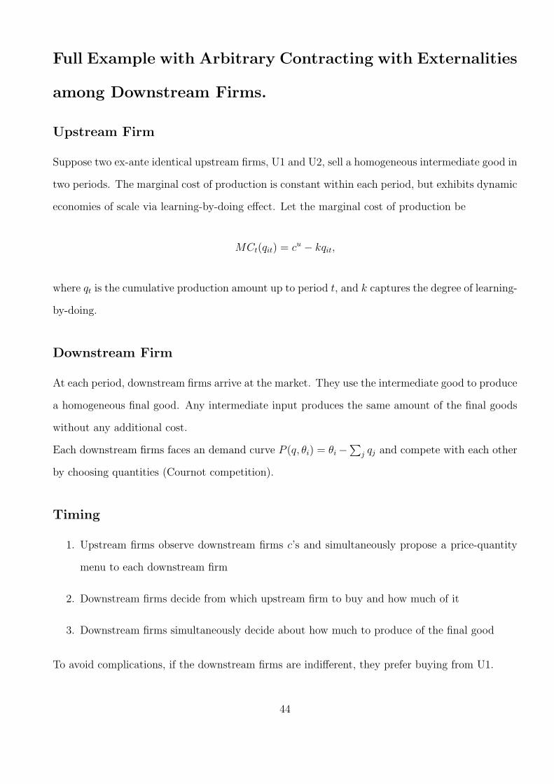
Full Example with Arbitrary Contracting with Externalities

among Downstream Firms.

Upstream Firm

Suppose two ex-ante identical upstream firms, U1 and U2, sell a homogeneous intermediate good in

two periods. The marginal cost of production is constant within each period, but exhibits dynamic

economies of scale via learning-by-doing effect. Let the marginal cost of production be

MCt(qit) = cu − kqit,

where qt is the cumulative production amount up to period t, and k captures the degree of learning-

by-doing.

Downstream Firm

At each period, downstream firms arrive at the market. They use the intermediate good to produce

a homogeneous final good. Any intermediate input produces the same amount of the final goods

without any additional cost.

Each downstream firms faces an demand curve P (q, θi) = θi−∑

j qj and compete with each other

by choosing quantities (Cournot competition).

Timing

1. Upstream firms observe downstream firms c’s and simultaneously propose a price-quantity

menu to each downstream firm

2. Downstream firms decide from which upstream firm to buy and how much of it

3. Downstream firms simultaneously decide about how much to produce of the final good

To avoid complications, if the downstream firms are indifferent, they prefer buying from U1.

44

Example

Suppose

period 1 2 downstream firms D1 with θ1 and D2 with θ2 arrive. (θ1 > θ2)

period 2 2 downstream firms D3 with θ1 and D4 with θ2 arrive. (θ1 > θ2)

What Social Planner would do.

Given a total production amount of the intermediate good, the social planner allocates the inter-

mediate good to maximize total welfare. Since the total welfare can be described as

(θ1 − (q1 + q2)

)q1 +

(θ2 − (q1 + q2)

)q2,

in the allocation that maximize the total welfare, one downstream firm with the highest θ use

all of the intermediate good. This result characterizes the social planner’s solution in the inter-

mediate good allocation. In the intermediate production, since there exists a learning-by-doing

effect, the production cost of intermediate good is minimized when one upstream firm does all the

production for any amount of total production, which characterize the social planner’s problem in

the intermediate good production. Therefore, at each period, one upstream firm produces all the

intermediate good and one downstream firm with the highest θ produces all the final goods up to

the point where P (Qt, θ) = θ −Qt = Long-run marginal cost of the intermediate good.

Equilibrium with Arbitrary Pricing Menu

By backward induction.

2nd Period

Let Q1 and Q2 be the production quantity of U1 and U2 in the 1st period. Let Q1 > Q2.

The following consists an equilibrium.

1. U2 propose a simple linear pricing menu p(q) = q × (cu − kQ2) to both downstream firms.

2. U1 propose (1) a simple linear pricing menu p(q) = q× (cu − kQ2) to D4 and (2) two part tariff

45

p(q) = F2(Q1, Q2) + q × (cu − kQ1) to D3, where

F2(Q1, Q2) =1

4

{k2(Q2

1 −Q22) + 2k(Q1 −Q2) (θ1 − cu)

}.

In the equilibrium, the dominant upstream firm produces all the intermediate good. Since the

dominant upstream firm has lower marginal cost, it can always undercut the rival’s price. In the

downstream market, D3 act as if its marginal cost is cu− kQ2 and D4 act as if its marginal cost is

cu − kQ1. Since U1 makes the menu to maximize industry profit and tries to extract it all by two

part tariff, U1 under-supply to D4. And U1 sets the marginal price equals to the true marginal

cost to D3 so that D3 maximize the profit in the downstream market. However, the amount of

the profit that U1 can extract is constrained by the fact that both downstream firms can deviate

from U1’s menu and by the intermediate good from U2. The maximum amount of profit that U1

can extract is defined by F2(Q1, Q2).

1st Period

Given the analysis above, I next explain the equilibrium in the first period. First, let me describe

the equilibrium.

The following consists an equilibrium.

1. U1 propose (1) simple linear pricing menu p(q) = qcu to D2 and (2) non-linear pricing p(q) =

qcu − F2(q∗1 + q, 0) to D2, where q∗1 is the equilibrium quantity D1 chooses.

2. U2 propose the same price-quantity menu as U1.

The equilibrium pricing maximizes the industry profit subject to the fact that one of the upstream

firms can always supply the intermediate good to downstream firms at the cost of cu. Since

downstream firms favor U1, in equilibrium, one upstream firm (U1) produces all the intermediate

good and designs the menu to maximize the joint surplus of U1 and the downstream firms.

46