quantlib erlk onige › slides › qlws14 › caspers.pdf · formula (i.e. hagan 2002) over a...

QuantLib Erlkonige

Peter Caspers

IKB

December 4th 2014

Peter Caspers (IKB) QuantLib Erlkonige December 4th 2014 1 / 47

Erlkonig


Table of contents

1 No Arbitrage SABR

2 ZABR, SVI

3 Linear TSR CMS Coupon Pricer

4 CMS Spread Coupons

5 Credit Risk Plus

6 Gaussian1d Models

7 Simulated Annealing

8 Runge Kutta ODE Solver

9 Dynamic Creator of Mersenne Twister

10 Questions


No Arbitrage SABR

No Arbitrage SABR - the model

Paul Doust, No-arbitrage SABR, Journal of Computational Finance,Volume 15 / Number 3, Spring 2012. Main Features:

1 approximates the density (with a positive function), thereby producingan arbitrage free smile over strike range [0,∞)

2 assumes arbsorbing barrier at F = 0 and reproduces precomputedarbsorption probabilities generated by a MC simulation (published byPaul Doust as well)

3 call prices are computed by numerical integration, implied volatilitiesare computed by inverting the Black formula


No Arbitrage SABR

No Arbitrage SABR Example

-40

-30

-20

-10

0

10

20

30

40

0 0.02 0.04 0.06 0.08 0.1 0.12 0.14

den

sity

strike

Hagan (2002)Doust

Figure : SABR smile α = 0.02, β = 0.40, ν = 0.30, ρ = 0.30, τ = 30.0, f = 0.03


No Arbitrage SABR

No Arbitrage SABR classes

ql/experimental/volatility/

NoArbSabrModel core computation formulasNoArbSabrInterpolation interpolation classNoArbSabrSmileSection smile section by parametersNoArbSabrInterpolatedSmileSection interpolating smile sectionSwaptionVolcube1a volatility cube


No Arbitrage SABR

Design changes

Make the SABR interpolation and volatility cube classes generic, so thatboth models (and possibly more like SVI, ZABR) are accepted. The oldSwaptionVolCube1 class e.g. is now retrieved by

struct SwaptionVolCubeSabrModel {

typedef SABRInterpolation Interpolation;

typedef SabrSmileSection SmileSection;

};

typedef SwaptionVolCube1x<SwaptionVolCubeSabrModel>

SwaptionVolCube1;

and likewise for the new “1a”-variant of the cube using the noarb-SABRformula.


No Arbitrage SABR

NoArbSABR - limitations

1 there are examples of parameters (α, β, ν, ρ) for which therecalibration of the model implied forward does not work

2 the implied volatility (since inverted from call prices) is not smoothfor far otm strikes in some cases (but actually rarely needed becausecalls, digitals and the density is directly available !)

3 in general, never underestimate the benefit of a pure closed formformula (i.e. Hagan 2002) over a computation involving numericalprocedures ...


ZABR, SVI

ZABR, SVI

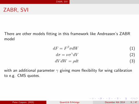
There are other models fitting in this framework like Andreasen’s ZABRmodel

dF = F βσdW (1)

dσ = νσγdV (2)

dV dW = ρdt (3)

with an additional parameter γ giving more flexibility for wing calibrationto e.g. CMS quotes.


ZABR, SVI

ZABR Example

0.1

0.2

0.3

0.4

0.5

0.6

0.7

0.8

0.9

0 0.1 0.2 0.3 0.4 0.5 0.6 0.7

imp

lied

logn

orm

alvo

lati

lity

strike

SABRZABR 1.0ZABR 0.5ZABR 1.5

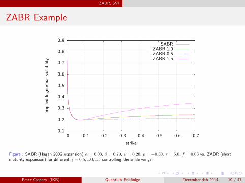
Figure : SABR (Hagan 2002 expansion) α = 0.03, β = 0.70, ν = 0.20, ρ = −0.30, τ = 5.0, f = 0.03 vs. ZABR (shortmaturity expansion) for different γ = 0.5, 1.0, 1.5 controlling the smile wings.


ZABR, SVI

ZABR - more features and limitations

1 two short maturity expansions (normal and lognormal impliedvolatility)

2 an “equivalent” Dupire - style FD approximation, which is fast andarbitrage free in particular

3 a full finite solution, for benchmarking and testing (slow of course)

4 but ... approximations are not very good for long option expiries

5 advantages for CMS pricing yet to be proved in a productive setting


ZABR, SVI

SVI

SVI is another popular smile model, with the total variance given by

v2t = a+ b(ρ(k −m) +

√(k −m)2 + σ2

)(4)

with log moneyness k = logK/F , K = strike, F = forward.


ZABR, SVI

SVI Example

0.2

0.25

0.3

0.35

0.4

0.45

0.5

0.55

0.6

0.65

0 0.01 0.02 0.03 0.04 0.05 0.06 0.07 0.08 0.09 0.1

imp

lied

logn

orm

alvo

lati

lity

strike

InputSVI

Figure : SVI fit to sample input data generated by SABR (α = 0.08, β = 0.90, ν = 0.30, ρ = 0.30, τ = 10.0, f = 0.03)


ZABR, SVI

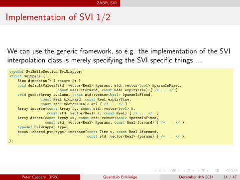
Implementation of SVI 1/2

We can use the generic framework, so e.g. the implementation of the SVIinterpolation class is merely specifying the SVI specific things ...

typedef SviSmileSection SviWrapper;

struct SviSpecs {

Size dimension() { return 5; }

void defaultValues(std::vector<Real> &params, std::vector<bool> &paramIsFixed,

const Real &forward, const Real expiryTime) { /* ... */ }

void guess(Array &values, const std::vector<bool> &paramIsFixed,

const Real &forward, const Real expiryTime,

const std::vector<Real> &r) { /* ... */ }

Array inverse(const Array &y, const std::vector<bool> &,

const std::vector<Real> &, const Real) { /* ... */ }

Array direct(const Array &x, const std::vector<bool> &paramIsFixed,

const std::vector<Real> &params, const Real forward) { /* ... */ }

typedef SviWrapper type;

boost::shared_ptr<type> instance(const Time t, const Real &forward,

const std::vector<Real> &params) { /* ... */ }

};


ZABR, SVI

Implementation of SVI (2/2)

... and use this in the generic implemenation:

class SviInterpolation : public Interpolation {

public:

template <class I1, class I2>

SviInterpolation(const I1 &xBegin, ... ) {

impl_ = boost::shared_ptr<Interpolation::Impl>(

new detail::XABRInterpolationImpl<I1, I2, detail::SviSpecs>(

xBegin, xEnd, yBegin, t, forward,

boost::assign::list_of(a)(b)(sigma)(rho)(m),

boost::assign::list_of(aIsFixed)(bIsFixed)(sigmaIsFixed)(

rhoIsFixed)(mIsFixed),

vegaWeighted, endCriteria, optMethod, errorAccept, useMaxError,

maxGuesses));

coeffs_ = boost::dynamic_pointer_cast<

detail::XABRCoeffHolder<detail::SviSpecs> >(impl_);

}

Note that XABR... is already to narrow as the label for the generic class.Better than the other way round ...


ZABR, SVI

SVI - limitations

1 uses the “raw” parametrization, which does not allow for easyparameter interpretation

2 calibration is naive, i.e. does not avoid local minima / parameteridentifcation problem cases


ZABR, SVI

Other smile models, general thoughts

There are other models, that are not fitted, but interpolate given points byconstruction such that the resulting smile is arbitrage free, e.g.

1 KahaleSmileSection which is already used implicity by the Markovfunctional model

2 BDK which fixes arbitrageable wings and introduce new parametersfor wing calibration

Goal: Integrate them as well in a uniform infrastructure providing

1 an interpolation class

2 a smile section which takes either parameters, market data or asource smile section to be smoothed / made arb-free

3 a swaption volatility cube with the possibility to calibrate to the cmsmarket and a caplet volatility surface


Linear TSR CMS Coupon Pricer

TSR CMS Coupon Pricers

A terminal swap rate (TSR) model is given by a mapping α

α(S(t)) =P (t, tP )

A(t)(5)

where tp is the coupon payment date and A(t) the annuity of theunderlying swap rate S. Then (integration by parts) the npv of a generalCMS coupon A(0)EA(P (t, tp)A(t)

−1g(S(t))) is given by

A(0)S(0)α(S(0)) +

∫ S(0)

−∞w(k)R(k)dk +

∫ ∞S(0)

w(k)P (k)dk (6)

with t begin the fixing date of the coupon, R and P prices of marketreceiver and payer swaptions and weights w(s) = {α(s)g(s)}′′.



Hagan non parallel shifts model

In Hagan’s classic paper, the model A.4 “non parallel shifts” correspondsto the following choice of α

α(S) =Se−|h(tp)−h(t)|x

1− P (0,tn)P (0,t) e

−|h(tn)−h(t)|x(7)

with tn being the last payment date of the underyling swap and

h(s)− h(t) = 1−e−κ(s−t)κ with a mean reversion parameter κ and x

implicitly given by

S(t)∑

τjP (0, tj)e−|h(tj)−h(t)|x + P (0, tn)e

−|h(tn)−h(t)|x = P (0, t) (8)

with τj , tj being the yearfractions and payment dates of the fixed leg ofthe underlying swap.



Linear TSR model

The linear terminal swap rate model is defined by

α(S) = as+ b (9)

b is determined by the no arbitrage condition

P (0, tp)/A(0) = EA(P (t, tp)/A(t)) = aS(0) + b (10)

a can be specified indirectly via a reversion κ by setting

a =∂

∂S(t)

P (t, tp)

A(t)(11)

and evaluating the r.h.s. within a one factor gaussian model.



Put Call Parity Example

1e-18

1e-16

1e-14

1e-12

1e-10

1e-08

1e-06

1e-04

0 0.01 0.02 0.03 0.04 0.05 0.06 0.07 0.08 0.09 0.1

pu

tca

llp

arit

yvi

olat

ion

strike

Hagan (Numeric, NonParallelShifts)Linear TSR

Figure : Parity error for a CMS10y coupon with in arrears fixing in 10y from today, Forward is 0.03, Volatility is given by aSABR surface with α = 0.10, β = 0.80, ν = 0.40, ρ = −0.30, reversion is zero, Integration Accuracy for the Linear TSRpricer is 10−10



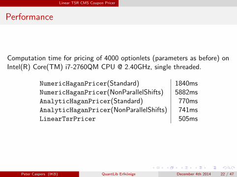
Performance

Computation time for pricing of 4000 optionlets (parameters as before) onIntel(R) Core(TM) i7-2760QM CPU @ 2.40GHz, single threaded.

NumericHaganPricer(Standard) 1840msNumericHaganPricer(NonParallelShifts) 5882msAnalyticHaganPricer(Standard) 770msAnalyticHaganPricer(NonParallelShifts) 741msLinearTsrPricer 505ms



Fast Erlkonig


CMS Spread Coupons

CMS Spread Coupons

Still missing: a coupon class which models cms spread coupons

τ(CMS10y− CMS2y) (12)

possibly capped and / or floored.


CMS Spread Coupons

Approach 1: Formula index

Introduce an artificial index derived from InterestRateIndex

SwapSpreadIndex(const std::string& familyName,

const boost::shared_ptr<SwapIndex>& swapIndex1,

const boost::shared_ptr<SwapIndex>& swapIndex2,

const Real gearing1 = 1.0,

const Real gearing2 = -1.0);

and build everything else on top of it as with the other coupons based onibor or cms indexes.


CMS Spread Coupons

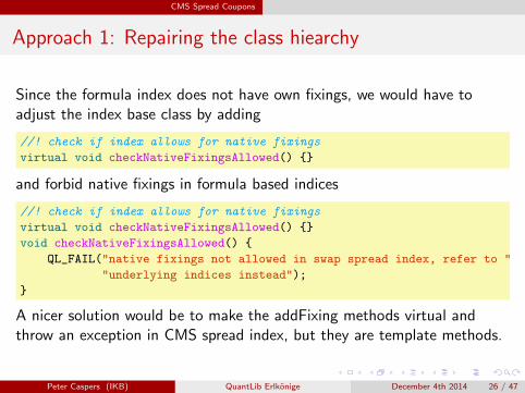
Approach 1: Repairing the class hiearchy

Since the formula index does not have own fixings, we would have toadjust the index base class by adding

//! check if index allows for native fixings

virtual void checkNativeFixingsAllowed() {}

and forbid native fixings in formula based indices

//! check if index allows for native fixings

virtual void checkNativeFixingsAllowed() {}

void checkNativeFixingsAllowed() {

QL_FAIL("native fixings not allowed in swap spread index, refer to "

"underlying indices instead");

}

A nicer solution would be to make the addFixing methods virtual andthrow an exception in CMS spread index, but they are template methods.


CMS Spread Coupons

Approach 2: Construct coupons with two swap indexes

If two swap indexes are used to construct a cms spread coupon we wouldneed a more flexible way to construct floating legs, since

template <typename InterestRateIndexType,

typename FloatingCouponType,

typename CappedFlooredCouponType>

Leg FloatingLeg(const Schedule& schedule,

const std::vector<Real>& nominals,

const boost::shared_ptr<InterestRateIndexType>& index,

const DayCounter& paymentDayCounter,

BusinessDayConvention paymentAdj,

const std::vector<Natural>& fixingDays,

const std::vector<Real>& gearings,

const std::vector<Spread>& spreads,

const std::vector<Rate>& caps,

const std::vector<Rate>& floors,

bool isInArrears, bool isZero) {

only allows for one index.


CMS Spread Coupons

Approach 2: Coupon Factories

We could introduce a factory instead of the template parameters

Leg FloatingLeg(const FloatingCouponFactory& factory,

const Schedule& schedule,

...

which can generate plain, capped / floored and digital couons for the ibor,cms, cms spread flavours.

class FloatingCouponFactory {

virtual boost::shared_ptr<FloatingRateCoupon>

plainCoupon(const Date &paymentDate, Real nominal,...)

virtual boost::shared_ptr<CappedFlooredCoupon>

cappedFlooredCoupon(const Date &paymentDate, Real nominal,...)

virtual boost::shared_ptr<DigitalCoupon> digitalCoupon(

const Date &paymentDate, Real nominal, const Date &startDate,...)

virtual Natural defaultFixingDays() const = 0;

};


CMS Spread Coupons

CMS Spread Coupons - Summary

Introducing a formula based index would not exactly fit the semanticsof the Index class. We would have to distinguish between nativeindexes (with own fixings) and derived ones. On the other hand thisseems to be a quite generic approach, since formula based indexescould be used whereever an InterestRateIndex is allowed

Using two indexes in the spread coupon class forces us to introduce amore flexible way to construct floating legs, e.g. via factories. Thiskeeps the design clean and the semantics of index sharp. Howeverthis is not 100% backward compatible since FloatingLeg is in themain QuantLib namespace.


Credit Risk Plus

Credit Risk Plus

A single period, nominal based credit portfolio model, based on CreditRisk Plus, with some extensions allowing for correlated sectors (IntegratingCorrelations, Risk, July 1999).

CreditRiskPlus(const std::vector<Real> &exposure,

const std::vector<Real> &defaultProbability,

const std::vector<Size> &sector,

const std::vector<Real> &relativeDefaultVariance,

const Matrix &correlation, const Real unit);

The loss distribution is computed analytically, so very fast. The modelcomes with a decomposition of the unexpected loss into single obligors’marginal losses.


Gaussian1d Models

Gaussian1d Models

Framework for one factor models with the following interfacevirtual const Real numeraireImpl(const Time t, const Real y,

const Handle<YieldTermStructure> &yts) const = 0;

virtual const Real zerobondImpl(const Time T, const Time t,

const Real y,

const Handle<YieldTermStructure> &yts) const = 0;

Currently two instances exist

1 MarkovFunctional, a non parametric Markov functional model withpiecewise volatility and constant reversion

2 Gsr, a Hull White model with piecewise volatility and piecewisereversion


Gaussian1d Models

Gaussian1d Models - Features

1 multi-curve enabled

2 engines for standard swaptions, swaptions with non-constant nominal,rates, float-float swaptions

3 engines inherit from BasketGeneratingEngine that can generatecalibration baskets by npv-delta-gamma matching

4 engines take an OAS allowing for exotic bond valuation


Simulated Annealing

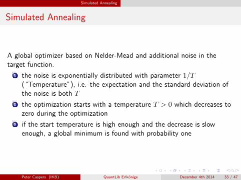
Simulated Annealing

A global optimizer based on Nelder-Mead and additional noise in thetarget function.

1 the noise is exponentially distributed with parameter 1/T(“Temperature”), i.e. the expectation and the standard deviation ofthe noise is both T

2 the optimization starts with a temperature T > 0 which decreases tozero during the optimization

3 if the start temperature is high enough and the decrease is slowenough, a global minimum is found with probability one


Simulated Annealing

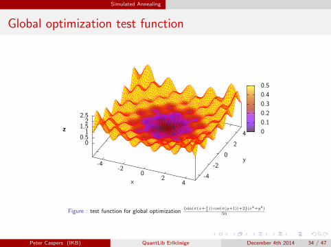
Global optimization test function

-4-2

02

4-4

-2

0

2

4

00.5

11.5

22.5

z

x

y

z 0

0.1

0.2

0.3

0.4

0.5

Figure : test function for global optimization{sin(π(x+ 1

2 )) cos(π(y+1))+2}(x2+y2)

50


Simulated Annealing

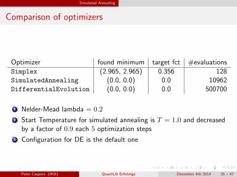
Comparison of optimizers

Optimizer found minimum target fct #evaluations

Simplex (2.965, 2.965) 0.356 128SimulatedAnnealing (0.0, 0.0) 0.0 10962DifferentialEvolution (0.0, 0.0) 0.0 500700

1 Nelder-Mead lambda = 0.2

2 Start Temperature for simulated annealing is T = 1.0 and decreasedby a factor of 0.9 each 5 optimization steps

3 Configuration for DE is the default one


Runge Kutta ODE Solver


An ODE solver using a forth order Runge Kutta scheme with adaptive stepsize control (as described in Numerical Recipes in C, Chapter 17.2). Itintegrates

d

dxf = F (x, f(x)) (13)

over an interval [a, b] for f : [a, b]→ Kn with K denoting the real orcomplex numbers with initial condition f(a) = fa.



Solving the modified Bessel equation

As an example we solve the modified Bessel equation

x2y′′ + xy′ − (x2 + α)y = 0 (14)

for α = 1 with y(0) = 0 and y′(0) = 0.5 over [0, 10] and compare it to theexpected result Iα(10) (modifiedBesselFunction_i).



Reduction to first derivatives

Equation 14 is equivalent to the system

y′ = z (15)

x2z′ + xz − (x2 + α)y = 0 (16)

with y(0) = 0 and z(0) = y′(0) = 0.5.



Code example for ODE solving

The ODE F can be defined as follows:

Disposable<std::vector<Real>> rhs(const double x,

const std::vector<Real> &f) {

std::vector<Real> result(2);

result[0] = f[1];

if (close(x, 0.0))

result[1] = (2.0 + alpha * alpha) * f[0] / 2.0;

else

result[1] = ((x * x + alpha * alpha) *

f[0] - x * f[1]) / (x * x);

return result;

}



Code example for ODE solving

To compute I1(10) we can then write

AdaptiveRungeKutta<Real> rk( 1e-16 );

std::vector<Real> y;

y += 0.0, 0.5;

Real i1 = rk( rhs, y , 0.0, 10.0 )[0];

with an ultra-tight tolerance here, just to see what is possible.



ODE solution vs. semi-analytical solution

1e-17

1e-16

1e-15

1e-14

1e-13

1e-12

1e-11

1e-10

0 2 4 6 8 10

erro

r

x

Figure : Runge Kutta adaptive step size solution with ε = 10−16 vs. modifiedBessel i


Dynamic Creator of Mersenne Twister


Makoto Matsumoto and Takuji Nishimura, “Dynamic Creation ofPseudorandom Number Generators” and their implementation as a Clibrary (http://www.math.sci.hiroshima-u.ac.jp/˜m-mat/MT/DC/dc.html)addresses two needs

1 create Mersenne Twister instances with smaller state space than theclassic instance (624 words of 32 bit) and smaller period than219937 − 1, or bigger ones if you really want ...

2 create “independent” Mersenne Twister intances for different id’s foruse in parralel monte carlo

The QuantLib wrapper support both dynamic creation of instances(MersenneTwisterDynamicRng) as well as the usage of precomputedinstances (MersenneTwisterCustomRng<Description>).



Instantiation of dynamic MT’s

Dynamically create an instance with 32 bit word size, p = 521, creatorseed 123, id 0 and seed 42:

MersenneTwisterDynamicRng mt(32,521, 123, 0, 42);

Use a precomputed instance with seed 42 (p is 19937 here, id is 0)

MersenneTwisterCustomRng<Mtdesc19937_0> mt(42);

The second alternative is much faster in random number generation. Alsoit takes a long time to dynamically create MT instances for bigger p.



Example: Parallel RNG streams

This code computes π using parallel mc with 8 threads

#define BOOST_PP_LOCAL_LIMITS (0, 7)

#define BOOST_PP_LOCAL_MACRO(n) MersenneTwisterCustomRng<Mtdesc19937_##n> mt##n(42);

#include BOOST_PP_LOCAL_ITERATE()

omp_set_num_threads(std::min(8, omp_get_max_threads()));

Real sum = 0.0;

Size N = 1E8;

#pragma omp parallel for reduction(+ : sum) schedule(static)

for (Size i = 0; i < N; ++i) {

Size thread = omp_get_thread_num();

Real u=0.0,v=0.0;

#define BOOST_PP_LOCAL_LIMITS (0, 7)

#define BOOST_PP_LOCAL_MACRO(n) if(thread==n) { u=mt##n.nextReal(); v=mt##n.nextReal(); }

#include BOOST_PP_LOCAL_ITERATE()

if(u*u+v*v <= 1.0) sum+=1;

}

std::cout << std::setprecision(8) << 4.0 * sum / N << std::endl;

Actually this does not run faster multithreaded due to compileroptimizations (vectorization) of the loop, nevertheless illustrates how touse it.



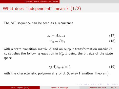
What does “independent” mean ? (1/2)

The MT sequence can be seen as a recurrence

sn = Asn−1 (17)

xn = Bsn (18)

with a state transition matrix A and an output transformation matrix B.sn satisfies the following equation in Fk2, k being the bit size of the statespace

χ(A)sn−k = 0 (19)

with the characteristic polynomial χ of A (Cayley Hamilton Theorem).



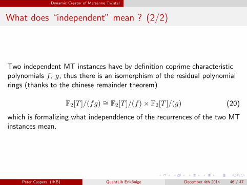
What does “independent” mean ? (2/2)

Two independent MT instances have by definition coprime characteristicpolynomials f , g, thus there is an isomorphism of the residual polynomialrings (thanks to the chinese remainder theorem)

F2[T ]/(fg) ∼= F2[T ]/(f)× F2[T ]/(g) (20)

which is formalizing what independdence of the recurrences of the two MTinstances mean.


Questions

Questions / Discussion

French Erlkonig


quantlib erlk onige › slides › qlws14 › caspers.pdf · formula (i.e. hagan 2002) over a...

Documents