quantum bayesian networks with application to games
TRANSCRIPT

Quantum Bayesian networks with application to games displaying Parrondo’sparadox
by
Michael Pejic
A dissertation submitted in partial satisfaction of the
requirements for the degree of
Doctor of Philosophy
in
Mathematics
in the
Graduate Division
of the
University of California, Berkeley
Committee in charge:
Professor F. Alberto Grunbaum, ChairProfessor Nicolai Reshetikhin
Umesh Vazirani
Fall 2014

Quantum Bayesian networks with application to games displaying Parrondo’sparadox
Copyright 2014by
Michael Pejic
1
Abstract
Quantum Bayesian networks with application to games displaying Parrondo’s paradox
by
Michael Pejic
Doctor of Philosophy in Mathematics
University of California, Berkeley
Professor F. Alberto Grunbaum, Chair
Bayesian networks and their accompanying graphical models are widely used for predictionand analysis across many disciplines. We will reformulate these in terms of linear maps. Thisreformulation will suggest a natural extension, which we will show is equivalent to standardtextbook quantum mechanics. Therefore, this extension will be termed quantum. However,the term quantum should not be taken to imply this extension is necessarily only of utility insituations traditionally thought of as in the domain of quantum mechanics. In principle, itmay be employed in any modelling situation, say forecasting the weather or the stock market–it is up to experiment to determine if this extension is useful in practice. Even restrictingto the domain of quantum mechanics, with this new formulation the advantages of Bayesiannetworks can be maintained for models incorporating quantum and mixed classical-quantumbehavior. The use of these will be illustrated by various basic examples.
Parrondo’s paradox refers to the situation where two, multi-round games with a fixedwinning criteria, both with probability greater than one-half for one player to win, arecombined. Using a possibly biased coin to determine the rule to employ for each round,paradoxically, the previously losing player now wins the combined game with probabilitygreater than one-half. Using the extended Bayesian networks, we will formulate and analyzeclassical observed, classical hidden, and quantum versions of a game that displays this para-dox, finding bounds for the discrepancy from naive expectations for the occurrence of theparadox. A quantum paradox inspired by Parrondo’s paradox will also be analyzed. We willprove a bound for the discrepancy from naive expectations for this paradox as well. Gamesinvolving quantum walks that achieve this bound will be presented.

i
To my parents.

ii
Contents
Contents ii
List of Figures iv
1 Introduction 1
I Quantum Bayesian networks 4
2 Bayesian networks-graphical models 52.1 Graphical models as the form in which information is presented . . . . . . . . . 52.2 Transition probability functions . . . . . . . . . . . . . . . . . . . . . . . . . . . . 82.3 Graphical models as constraints . . . . . . . . . . . . . . . . . . . . . . . . . . . . 102.4 Directed graphical models as tensor networks . . . . . . . . . . . . . . . . . . . . 112.5 The Copy map and restriction maps . . . . . . . . . . . . . . . . . . . . . . . . . 13
3 Hidden classic and quantum nodes 143.1 Principles of linearity and potential universality . . . . . . . . . . . . . . . . . . 143.2 Options I and II . . . . . . . . . . . . . . . . . . . . . . . . . . . . . . . . . . . . . 163.3 Quantum nodes . . . . . . . . . . . . . . . . . . . . . . . . . . . . . . . . . . . . . . 203.4 No quantum copying . . . . . . . . . . . . . . . . . . . . . . . . . . . . . . . . . . . 223.5 Embedding quantum models into classical ones . . . . . . . . . . . . . . . . . . . 263.6 Embedding classical models into quantum ones . . . . . . . . . . . . . . . . . . . 323.7 Classical physics . . . . . . . . . . . . . . . . . . . . . . . . . . . . . . . . . . . . . 333.8 Additional structures for Bayesian networks? . . . . . . . . . . . . . . . . . . . . 34
4 Constructing the networks 364.1 Graphical constructs and rules . . . . . . . . . . . . . . . . . . . . . . . . . . . . . 364.2 Data for the structures using Option I’ . . . . . . . . . . . . . . . . . . . . . . . . 374.3 Data for the structures using Option II . . . . . . . . . . . . . . . . . . . . . . . 384.4 Example-double-slit experiment . . . . . . . . . . . . . . . . . . . . . . . . . . . . 394.5 Quantum model . . . . . . . . . . . . . . . . . . . . . . . . . . . . . . . . . . . . . 404.6 The Bayesian network approach versus the standard textbook approach . . . . 42

iii
4.7 Classical hidden model . . . . . . . . . . . . . . . . . . . . . . . . . . . . . . . . . 434.8 What is a quantum system? . . . . . . . . . . . . . . . . . . . . . . . . . . . . . . 45
5 Relation to textbook quantum mechanics 465.1 Textbook rules for quantum mechanics . . . . . . . . . . . . . . . . . . . . . . . . 465.2 Weak measurements . . . . . . . . . . . . . . . . . . . . . . . . . . . . . . . . . . . 525.3 Comparison of Bayesian networks to quantum circuits and tensor networks . . 54
6 Further examples 566.1 No-cloning–classical and quantum . . . . . . . . . . . . . . . . . . . . . . . . . . . 566.2 Teleportation-classical and quantum . . . . . . . . . . . . . . . . . . . . . . . . . 576.3 Bell’s inequality for Bayesian networks without metaphysical limitations . . . 60
II Parrondo’s paradox and a Parrondo-like paradox 64
7 Parrondo’s paradox 657.1 Defining the paradox . . . . . . . . . . . . . . . . . . . . . . . . . . . . . . . . . . 657.2 Classical observed Markov chain game . . . . . . . . . . . . . . . . . . . . . . . . 667.3 Classical hidden-Markov chain game . . . . . . . . . . . . . . . . . . . . . . . . . 707.4 Defining a quantum analogue of the Markov model . . . . . . . . . . . . . . . . 757.5 Parrondo’s paradox for the quantum game . . . . . . . . . . . . . . . . . . . . . 807.6 Summary of results . . . . . . . . . . . . . . . . . . . . . . . . . . . . . . . . . . . 83
8 A Parrondo-like paradox for an one-round game 868.1 Defining the game . . . . . . . . . . . . . . . . . . . . . . . . . . . . . . . . . . . . 868.2 Defining geodesics on the space of wavefunctions . . . . . . . . . . . . . . . . . . 878.3 Bounds on the extent of the Parrondo-like paradox . . . . . . . . . . . . . . . . 898.4 Conditions for the occurrence of the Parrondo-like paradox . . . . . . . . . . . 92
9 Quantum walks and the Parrondo-like paradox 959.1 Classical random and classical hidden walks . . . . . . . . . . . . . . . . . . . . . 959.2 Quantum walks . . . . . . . . . . . . . . . . . . . . . . . . . . . . . . . . . . . . . . 999.3 The Parrondo-like paradox for quantum walks . . . . . . . . . . . . . . . . . . . 104
Bibliography 109
A General propositions 114A.1 Banach space propositions . . . . . . . . . . . . . . . . . . . . . . . . . . . . . . . 114A.2 Hilbert space propositions . . . . . . . . . . . . . . . . . . . . . . . . . . . . . . . 115A.3 Transition function propositions . . . . . . . . . . . . . . . . . . . . . . . . . . . . 116
B Propositions for option I 119
iv
B.1 Measures . . . . . . . . . . . . . . . . . . . . . . . . . . . . . . . . . . . . . . . . . . 119B.2 Maps on subspaces of the space of measures . . . . . . . . . . . . . . . . . . . . . 121B.3 L1-spaces . . . . . . . . . . . . . . . . . . . . . . . . . . . . . . . . . . . . . . . . . 128B.4 Density-matrix-valued L1-spaces . . . . . . . . . . . . . . . . . . . . . . . . . . . . 128B.5 Maps on density-matrix-valued L1-spaces . . . . . . . . . . . . . . . . . . . . . . 129B.6 Vector measures . . . . . . . . . . . . . . . . . . . . . . . . . . . . . . . . . . . . . 139
C Propositions for option II 141C.1 Real-valued, continuous functions . . . . . . . . . . . . . . . . . . . . . . . . . . . 141C.2 Maps on real-valued, continuous functions . . . . . . . . . . . . . . . . . . . . . . 142C.3 Compact-operator-valued, continuous functions . . . . . . . . . . . . . . . . . . . 146C.4 Operator inequalities . . . . . . . . . . . . . . . . . . . . . . . . . . . . . . . . . . 146C.5 Maps on compact-operator-valued, continuous functions . . . . . . . . . . . . . 150
List of Figures
7.1 Minimum achievable values of P combA for p = 0.5 for the two-state, classical hidden
game. . . . . . . . . . . . . . . . . . . . . . . . . . . . . . . . . . . . . . . . . . . . . . . 847.2 Minimum achievable values of P comb
A for p = 0.1 for the two-state, classical hiddengame. . . . . . . . . . . . . . . . . . . . . . . . . . . . . . . . . . . . . . . . . . . . . . . 84
7.3 Minimum achievable values of P combA for p = 0.5 for the two-dimensional, quantum
game. . . . . . . . . . . . . . . . . . . . . . . . . . . . . . . . . . . . . . . . . . . . . . . 857.4 Minimum achievable values of P comb
A for p = 0.1 for the two-dimensional, quantumgame. . . . . . . . . . . . . . . . . . . . . . . . . . . . . . . . . . . . . . . . . . . . . . . 85

v
Acknowledgments
Michael Pejic acknowledges support from the Applied Math. Sciences subprogram of theOffice of Energy Research, US Department of Energy, under Contract DE-AC03-76SF00098,and from AFOSR grant FA95501210087 through a subcontract to Carnegie Mellon Univer-sity.

1
Chapter 1
Introduction
Outline of the work
Bayesian networks and graphical models are useful for classical systems because they aremuch more intuitive than a list of conditional dependencies. It is also sometimes useful tointroduce additional, hypothesized nodes to break complicated dependencies into simpler,potentially universal modules. Usually these are treated just as observable nodes whichare always hidden; however, this imposes constraints that are metaphysical in origin andraises difficulties of interpretation. We will give an alternate approach using linear mapson measures, with additional constructions to those generally utilized in graphical models,that resolves those issues. While, in certain situations, this introduces additional maps, notpreviously available, these new maps are not only in and of themselves of limited interest,but also introduce undesired complications. However, what is extremely fruitful is simply theconceptual leap. Thinking in terms of linear maps on spaces of measures immediately raisesthe question of looking at linear maps on other spaces. This approach leads to a natural ex-tension, which we will prove is equivalent to standard, textbook quantum mechanics (whichis infamous for its apparently unmotivated and incomprehensible formulation). Therefore,this extension will be termed quantum. To avoid being swept away by a flood of details,propositions of a more general nature, together with their proofs, needed to show the sensi-bility and consistency of the extension and its equivalence to quantum mechanics are placedin appendices.
However, the term quantum should not be taken to imply this extension is necessarilyonly of utility in situations traditionally thought of as in the domain of quantum mechanics.In principle, it may be employed in any modelling situation, say forecasting weather orstock prices–it is up to experiment to determine if this extension is useful in practice. Inparticular, there is no reason for h to necessarily enter into these models if they are outsidethe realm of physics. Even restricting to the traditional domain of quantum mechanics, withthis new formulation the advantages of Bayesian networks can be maintained for modelsincorporating quantum and mixed classical-quantum behavior. The use of these will beillustrated by various examples. In particular, we will show that some of the supposed
CHAPTER 1. INTRODUCTION 2
hallmarks of quantum mechanics, no-cloning and teleportation, apply for classical hiddensystems as well.
In the second part, we will utilize these extended Bayesian networks in the study ofvarious games displaying Parrondo’s paradox–the phenomenon of two games each winningfor one player with probability greater than one-half, yet their convex combination (in asense to be specified) paradoxically winning for the previously losing player with probabilitygreater than one-half. We will prove bounds for the discrepancy from naive expectations forclassical versions of a game; those bounds will then be shown to be broken by a quantumanalogue of the game. [26]
A quantum paradox inspired by Parrondo’s paradox will also be analyzed. We will provea bound for the discrepancy from naive expectations for this paradox. Games involvingquantum walks that achieve this bound will be presented.
Philosophical interlude–rejection of metaphysics
For a man will attain unto nothing more perfect than to be found to be mostlearned in the ignorance which is distinctly his. The more he knows that he isunknowing, the more learned he will be.–Nicholas of Cusa [27]
The philosophy we employ in this work is one with a long-standing pedigree: we know nothingabout underlying reality and, therefore, any claims about it or appeals to it are invalid. Thereis no reason to believe reality is doing calculations at all similar to the ones we employ inour hypothesized models or even that it is doing calculations at all. In particular there is theissue of contextuality–we want to employ potentially universal modules in our models sinceonly they have predictive ability in novel situations, but perhaps reality is fundamentallycontextual.
Constraints imposed on our models
In keeping with the expressed philosophy, no metaphysical constraints will be placed uponthe mathematical operations and constructs that can be employed in the models. Rather,there are only three rules that will be enforced. Firstly, the quantities calculated by themathematical models must be interpretable as probabilities; in particular, they must bepositive1. Secondly, the mathematical models must be composed of linear maps (which wewill show is the weakening of a principle already in wide use, if not always acknowledged).Thirdly, the mathematical models must be composed of potentially universal modules (ina manner that we will precisely define). Of course, the particular model employed in aparticular situation may fail to be universal when actually employed in a different context;the point is that this failure should be as a result of experiment and not be preordained asresult of our choice of mathematics employed in modelling.
1To aid readability, positive is used instead of nonnegative throughout. Wherever strict positivity isrequired, the word strict will be added.

CHAPTER 1. INTRODUCTION 3
These constraints are extremely restrictive. For maps to be linear, they must clearlylive on linear spaces. Furthermore, they also impose strong restrictions on the linear spacesthese maps live on. Thus far, we are only aware of three classes of linear spaces that meetthe imposed restrictions: (i) certain subspaces of measures; (ii) density matrices on complexHilbert spaces ; (ii) and their tensor products. The former gives what is traditionally thoughtof as classical behavior and we will prove the latter two give behavior that has traditionallybeen taken the domain of quantum mechanics. However, since we do not start from quantummechanics, but instead only from the above principles, models involving maps on densitymatrices may be found to be of utility in situations not traditionally thought of as relatedto quantum mechanics.
4
Part I
Quantum Bayesian networks

5
Chapter 2
Bayesian networks-graphical models
2.1 Graphical models as the form in which
information is presented
There are many ways to present joint probability in terms of other quantities and mathemat-ical constructs. Graphical models [28] are a useful way to sort through what otherwise canseem hopelessly complicated in the usual notation. For instance, given a probability space(Ω,E , π) with two generalized random variables, X ∶ Ω → X and Y ∶ Ω → Y for sets X andY, then for any A ∈ X(E) and B ∈ Y (E), the joint probability Prob(X ∈ A and Y ∈ B) isπ (X−1(A)∩Y −1(B)). The graphical model corresponding to presenting the joint probabilityin this manner–namely by giving (Ω, E , π, X , X, Y, Y )–is
m mm
X
Ω
Y
/
SSSSw
SSSS
(2.1)
where the double arrows stand for deterministic causation.The resulting joint probability determines a probability space (X × Y,F , ρ) with the
probability measure ρ given on rectangular subsets by ρ(A×B) = Prob (X−1(A)∪ Y −1(B)),which can then be extended to a probability measure for the σ-algebra1 F generated by therectangular subsets on X × Y. The graphical model corresponding to presenting the jointprobability in this manner–namely by giving (X × Y, F , ρ)–is
m mX Y(2.2)
1A σ-algebra is a collection of subsets of a set X , including both ∅ and X , that is closed under relativecomplementation and countable unions.
CHAPTER 2. BAYESIAN NETWORKS-GRAPHICAL MODELS 6
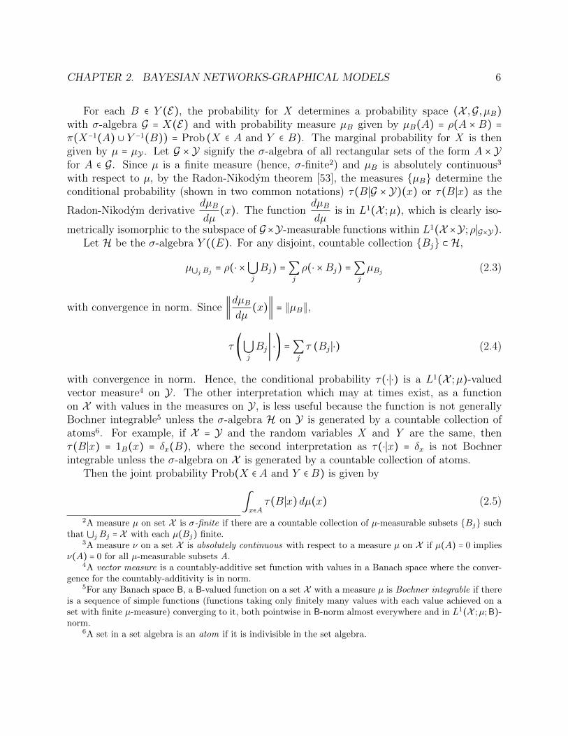
For each B ∈ Y (E), the probability for X determines a probability space (X ,G, µB)with σ-algebra G = X(E) and with probability measure µB given by µB(A) = ρ(A × B) =π(X−1(A) ∪ Y −1(B)) = Prob (X ∈ A and Y ∈ B). The marginal probability for X is thengiven by µ = µY . Let G × Y signify the σ-algebra of all rectangular sets of the form A × Yfor A ∈ G. Since µ is a finite measure (hence, σ-finite2) and µB is absolutely continuous3
with respect to µ, by the Radon-Nikodym theorem [53], the measures µB determine theconditional probability (shown in two common notations) τ(B∣G × Y)(x) or τ(B∣x) as the
Radon-Nikodym derivativedµBdµ
(x). The functiondµBdµ
is in L1(X ;µ), which is clearly iso-
metrically isomorphic to the subspace of G×Y-measurable functions within L1(X ×Y;ρ∣G×Y).Let H be the σ-algebra Y ((E). For any disjoint, countable collection Bj ⊂ H,
µ⋃j Bj = ρ(⋅ ×⋃j
Bj) =∑j
ρ(⋅ ×Bj) =∑j
µBj (2.3)
with convergence in norm. Since ∥dµBdµ
(x)∥ = ∥µB∥,
τ (⋃j
Bj∣ ⋅) =∑j
τ (Bj ∣⋅) (2.4)
with convergence in norm. Hence, the conditional probability τ(⋅∣⋅) is a L1(X ;µ)-valuedvector measure4 on Y . The other interpretation which may at times exist, as a functionon X with values in the measures on Y, is less useful because the function is not generallyBochner integrable5 unless the σ-algebra H on Y is generated by a countable collection ofatoms6. For example, if X = Y and the random variables X and Y are the same, thenτ(B∣x) = 1B(x) = δx(B), where the second interpretation as τ(⋅∣x) = δx is not Bochnerintegrable unless the σ-algebra on X is generated by a countable collection of atoms.
Then the joint probability Prob(X ∈ A and Y ∈ B) is given by
∫x∈A
τ(B∣x)dµ(x) (2.5)
2A measure µ on set X is σ-finite if there are a countable collection of µ-measurable subsets Bj suchthat ⋃j Bj = X with each µ(Bj) finite.
3A measure ν on a set X is absolutely continuous with respect to a measure µ on X if µ(A) = 0 impliesν(A) = 0 for all µ-measurable subsets A.
4A vector measure is a countably-additive set function with values in a Banach space where the conver-gence for the countably-additivity is in norm.
5For any Banach space B, a B-valued function on a set X with a measure µ is Bochner integrable if thereis a sequence of simple functions (functions taking only finitely many values with each value achieved on aset with finite µ-measure) converging to it, both pointwise in B-norm almost everywhere and in L1(X ;µ;B)-norm.
6A set in a set algebra is an atom if it is indivisible in the set algebra.

CHAPTER 2. BAYESIAN NETWORKS-GRAPHICAL MODELS 7
The directed graphical model corresponding to presenting the joint probability in this manner–namely by giving (X , G, Y, H,µ, τ(⋅∣⋅))–is
m mX Y-
(2.6)
Let ν be the marginal probability for Y, ν(B) = ρ(X × B). Then τ(⋅∣⋅) is absolutelycontinuous with respect to ν in the sense that τ(B∣⋅) is the zero function for every B suchthat ν(B) = 0. However, unless we are in the common case where the σ-algebra on X isgenerated by a countable collection of atoms, L1(X ;µ) does not have the Radon-Nikodymproperty7 [77] (the example given above demonstrates this); hence, there is in general nof ∈ L1(Y;ν;L1(X ;µ)) (which by Fubini’s theorem [54] is the same as L1(X × Y;µ × ν) forthe product measure8 µ× ν) such that the joint probability Prob(X ∈ A and Y ∈ B) is givenby ∫(x,y)∈A×B f(x, y)d(µ × ν)(x, y).
Lastly, defining ζ(⋅∣⋅) symmetrically to τ(⋅∣⋅), the directed graphical model correspondingto presenting the joint probability
Prob(X ∈ A and Y ∈ B) = ∫y∈B
ζ(A∣y)dν(y) (2.7)
by giving the marginal probability ν and the conditional probability ζ(⋅∣⋅) is
m mX Y
(2.8)
As an example, consider calculating the conditional probability
Prob (Y ∈ B∣X ∈ A) = Prob(Y ∈ B and X ∈ A)Prob(X ∈ A) (2.9)
(for Prob(X ∈ A) ≠ 0–otherwise the joint probability does not determine the conditionalprobability) using the information presented in the manner corresponding to each of thefour graphical models (the filled circle indicates which node is being conditioned on):
mm
X ∈ A
Ω
Y
/
SSSSw
SSSS
π (X−1(A) ∩ Y −1(B))π (X−1(A))
(2.10)
7A Banach space B has the Radon-Nikodym property if, for any B-valued vector measure ν on a set Xwhich is absolutely continuous with respect to some σ-finite measure µ on X , there is a Bochner integrable,B-valued function, dν
dµ, such that ν(A) = ∫A
dνdµdµ for any ν-measurable A.
8Unfortunately, by convention the tensor product of measures is called the product measure and writtenusing × instead of the more appropriate ⊗ (however, see [81] for a use of the latter notation).

CHAPTER 2. BAYESIAN NETWORKS-GRAPHICAL MODELS 8
mX ∈ A Yρ (A ×B)ρ (A × Y)
(2.11)
mX ∈ A Y-∫x∈A τ(B∣x)dµ(x)
µ(A)(2.12)
mX ∈ A Y∫y∈B ζ(A∣y)dν(y)∫y∈Y ζ(A∣y)dν(y)
(2.13)
For instance, Bayes’ theorem is simply the calculation corresponding to the presentation ofinformation by the last graphical model.
A similar situation holds for any finite number of random variables [52], with a graphicalmodel with deterministic causation emanating from a fundamental, hidden probability space,a graphical model with a clique of all the nodes for the random variables, and various directedmodels with probabilistic causation. For the common case where the various σ-algebras aregenerated by finitely many atoms, the various measures become vectors, the conditionalprobabilities become stochastic matrices9 or tensors, and the integrations become sums.
2.2 Transition probability functions
Depending on how the information for the calculation of the joint probability is presented,we may imagine different ways of varying it. For (2.1), it is most natural to imagine indepen-dently varying the maps X and Y. For (2.2), there is nothing to independently vary otherthan the joint probability itself. For (2.6), we would like to imagine varying the marginalprobability µ and the conditional probability τ(⋅∣⋅) independently. This is a problem becausethe space τ(⋅∣⋅) lives in–the L1(X ;µ)-valued vector measures–depends on µ. This problemwill exist even in the commonly occurring case where the σ-algebra G is generated by acountable collection of atoms if µ is zero on some atom (other than the empty set), sincethen the conditional probability when conditioning on that atom is not well-defined.
One solution to this problem, following [52], is provided by introducing the followingnotion:
9A matrix is stochastic if all entries are either positive or zero and all column sums are one.

CHAPTER 2. BAYESIAN NETWORKS-GRAPHICAL MODELS 9
Definition 2.2.1 For σ-algebras G on X and H on Y, a function τ(⋅∣⋅) ∶ H × X → R is atransition probability function if: (i) for each x ∈ X , τ(⋅∣x) is a probability measure on Ywith event σ-algebra H; and (ii) for each B ∈ H, τ(B∣⋅) is a bounded, G-measurable functionon X .
By taking τ(⋅∣⋅) to be a transition probability function rather than a conditional probability,it is now possible to vary µ and τ(⋅∣⋅) independently. For a fixed choice of τ(⋅∣⋅), there is aconvex linear map L from probability measures on X to probability measures on Y given by
(Lµ)(B) = ∫x∈X
τ(B∣x)dµ(x) (2.14)
The map L extends to a linear map on more general measures and signed measures.
Removing metaphysical constraints
Imagining one can vary µ and keep the transition probability function τ(⋅∣⋅) fixed, there is anintuitive interpretation of τ(⋅∣⋅) as an idealized conditional probability10, with τ(B∣x) beingthe probability to observe B given the event x, even if the latter has probability zero oris not even in the event σ-algebra (although in this latter case it is constant within anyatom). This leads to a metaphysical notion of the actual existence of a variable taking anactual value with probability reflecting our ignorance of its value. This may be of value fornodes in a graphical model which are observable; however, it is common to add hypothesized,hidden nodes to a directed graphical model in order to (hopefully) break it up into smaller,more manageable pieces [29]. For these, there is no justification to necessarily limit oneselfto transition probability functions. Furthermore, the probabilities and conditional proba-bilities involving the hidden nodes lack any meaning in either the Bayesian or frequentistinterpretations–the word probability then only means positive and norm-one.
Another solution (among many others) to the above posed problem is therefore to takethe independently varied objects to be the marginal probability µ and the linear map L.Not all linear maps that take probability measures to probability measures are necessarilyinduced by some transition probability function as in (2.14) (however, they are all inducedby some pseudo-transition function–see B2.7, B2.8, and B2.9), so this generally introducesadditional maps. These additional maps, involving operations such as Lebesgue decompo-sition [55], are not in and of themselves of great interest; in fact the raise rather undesiredcomplications (see §3.2). Furthermore, in the common case where the σ-algebras are gen-erated by countably many atoms, any linear map is induced by some transition probabilityfunction, so there are no additional maps. However, what is fruitful is the conceptual shift;as will be explored in the following chapter, once we are thinking in terms of linear maps,we are immediately drawn to consider the question of looking at linear maps between spacesother than spaces of measures.
10As noted in [52].

CHAPTER 2. BAYESIAN NETWORKS-GRAPHICAL MODELS 10
2.3 Graphical models as constraints
In addition to showing the form in which information is presented, graphical models canalso show constraints on the information in a far simpler form than the usual notation. Forinstance, consider the Markov chain with three random variables X,Y,Z. For the graphicalmodel
m mmmX
Ω
Y Z
/
?
SSSSw
SSSS
(2.15)
with the joint probability Prob(X ∈ A and Y ∈ B and Z ∈ C) given by π (X−1(A)∩Y −1(B)∩Z−1(C)), it is necessary to explicitly add the constraint that for every C ∈ Z(E), the con-ditional probability τ(C ∣x, y) = dµC
dµ , for µC(A × B) = π (X−1(A) ∩ Y −1(B) ∩ Z−1(C)) andµ = µZ , is independent of x (in the almost-everywhere, probabilistic sense). If, as above, weimagine varying the maps X and Y, it is not at all clear how to do this while maintainingthe constraint.
Similarly, for the graphical model
m mm
X
Y
Z
SSSS
(2.16)
with the joint probability Prob(X ∈ A and Y ∈ B and Z ∈ C) given by ρ(A × B × C), itis necessary to explicitly add the constraint that for every C ∈ I = Z(E), the conditionalprobability τ(C ∣x, y) = dµC
dµ , for µC(A ×B) = ρ(A ×B × C) and µ = µZ , is independent of x(in the almost-everywhere, probabilistic sense). If, as above, we imagine varying the jointprobability ρ, it is not at all clear how to do this while maintaining the constraint.
However, consider the directed graphical model:
m m mXY
Z- -
(2.17)
which corresponds to presenting the information to calculate the joint probability as φ, η(⋅∣⋅),and τ(⋅∣⋅) where
Prob(X ∈ A,Y ∈ B, and Z ∈ C) = ∫(x,y)∈A×B
τ(C ∣y)dµ(x, y) = ∫y∈B
τ(C ∣y)dξ(y) (2.18)

CHAPTER 2. BAYESIAN NETWORKS-GRAPHICAL MODELS 11
for the marginal probabilities µ on X × Y and ξ on Y given by
µ(A ×B) = ∫x∈A
η(B∣x)dφ(x), ξ(B) = µ(X ×B) = ∫x∈X
η(B∣x)dφ(x) (2.19)
The restriction is that the conditional probability τ(⋅∣⋅) is independent of x (in the almost-everywhere, probabilistic sense). It is not necessary to give this constraint explicitly since itis indicated by the graphical model through the lack of an arrow directly from X to Z. If,as above, we take η(⋅∣⋅) and τ(⋅∣⋅) as transition probability functions instead of conditionalprobabilities, it is now easy to see how to vary φ, η(⋅∣⋅), and τ(⋅∣⋅) while maintaining theconstraint–namely, by only allowing τ(⋅∣⋅) that are independent of x.
Note if the wrong directed model is chosen, the constraint can be masked. For instance,for the graphical model
m mm
X
Y
Z
/ S
SSSo
(2.20)
which corresponds to presenting the information to calculate the joint probability as ν, θ(⋅∣⋅),and ζ(⋅∣⋅) where
Prob(X ∈ A,Y ∈ B, and Z ∈ C) = ∫(y,z)∈B×C
ζ(A∣y, z)dκ(y, z) (2.21)
for the marginal probability κ on Y ×Z given by
κ(B ×C) = ∫z∈C×
θ(B∣z)dν(z) (2.22)
Once again, it is necessary to explicitly add the constraint that for every C ∈ I, the condi-tional probability τ(C ∣x, y) = dµC
dµ , for µC(A×B) = ∫(y,z)∈B×C ζ(A∣y, z)dκ(y, z) and µ = µZ , is
independent of x (in the almost-everywhere, probabilistic sense).This can be readily generalized to more complicated graphical models–any graph that is
not simply a clique11 of all the nodes implies constraints on the allowed joint probabilities.In this manner the various dependencies are displayed in a far more intuitive manner thanthrough a long list of opaque constraints. Of course, it is always possible to impose additionalconstraints explicitly.
2.4 Directed graphical models as tensor networks
Tensor networks are a commonly employed, diagrammatic device for contracting tensors andvectors. For the common case where the various σ-algebras are generated by finitely many
11A clique is a group of nodes that are all connected to one another.
CHAPTER 2. BAYESIAN NETWORKS-GRAPHICAL MODELS 12
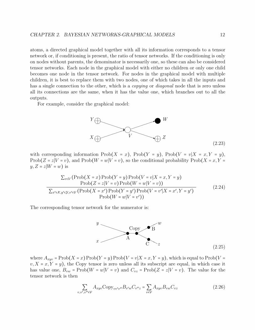
atoms, a directed graphical model together with all its information corresponds to a tensornetwork or, if conditioning is present, the ratio of tensor networks. If the conditioning is onlyon nodes without parents, the denominator is necessarily one, so these can also be consideredtensor networks. Each node in the graphical model with either no children or only one childbecomes one node in the tensor network. For nodes in the graphical model with multiplechildren, it is best to replace them with two nodes, one of which takes in all the inputs andhas a single connection to the other, which is a copying or diagonal node that is zero unlessall its connections are the same, when it has the value one, which branches out to all theoutputs.
For example, consider the graphical model:
mm
mm
X
Y
V Z
W
1
PPPPPPq
1
PPPPPPq
(2.23)
with corresponding information Prob(X = x), Prob(Y = y), Prob(V = v∣X = x,Y = y),Prob(Z = z∣V = v), and Prob(W = w∣V = v), so the conditional probability Prob(X = x,Y =y,Z = z∣W = w) is
∑v∈V (Prob(X = x)Prob(Y = y)Prob(V = v∣X = x,Y = y)Prob(Z = z∣V = v)Prob(W = w∣V = v))
∑x′∈X ,y′∈Y,v′∈V (Prob(X = x′)Prob(Y = y′)Prob(V = v′∣X = x′, Y = y′)Prob(W = w∣V = v′))
(2.24)
The corresponding tensor network for the numerator is:
v v vv
x
y
AC
BCopy
z
w
PPPPPPP
HHHHH
(2.25)
where Axyv = Prob(X = x)Prob(Y = y)Prob(V = v∣X = x,Y = y), which is equal to Prob(V =v,X = x,Y = y), the Copy tensor is zero unless all its subscript are equal, in which case ithas value one, Bvw = Prob(W = w∣V = v) and Cvz = Prob(Z = z∣V = v). The value for thetensor network is then
∑v,v′,v′′∈V
AxyvCopyvv′v′′Bv′wCv′′z =∑v∈V
AxyvBvwCvz (2.26)

CHAPTER 2. BAYESIAN NETWORKS-GRAPHICAL MODELS 13
which equals the numerator. For the denominator, the tensor network in this case is simply
v wD(2.27)
where
Dw = ∑x∈X ,y∈Y,v∈V
Prob(X = x)Prob(Y = y)Prob(V = v∣X = x,Y = y)Prob(W = w∣V = v)
(2.28)which is equal to Prob(W = w).
As this example illustrates, the advantages of the Bayesian network over the tensor net-work are that: (i) it is possible to show which nodes are being observed, marginalized, orconditioned on; and (ii) the nodes in the Bayesian network have a more intuitive interpre-tation. On the other hand, the tensor network does highlight the importance of copying forthere to be multiple child nodes, which will be important later for incorporating quantumnodes (see §3.2, §3.4, and §4.1).
2.5 The Copy map and restriction maps
Going along with the linear maps on measures induced by transition probability function(see (2.14)), we have the following additional useful linear maps for the evaluation of thejoint probability for a directed graphical model. For a set X with σ-algebra E , there isa Copy map from E-measures on X to F -measures on X × X , where F is the σ-algebragenerated by the rectangular sets E × E . It is given by, for any set A ∈ F and E-measureµ, Copy(µ)(A) = µ (x ∈ X ∣(x,x) ∈ A). It is induced by the transition probability functionτ(⋅∣⋅) given by
τ(A∣x) =⎧⎪⎪⎨⎪⎪⎩
1 if (x,x) ∈ A0 otherwise
(2.29)
This can clearly be generalized for creating any finite number of copies.For each A ∈ E , there is a restriction map, which is an idempotent, sending E-measures
on X to E-measures12 on X , µ → 1Aµ = µ(A ∩ ⋅). It is induced by the transition probabilityfunction τ(⋅∣⋅) given by τ(A∣x) = 1A(x).
12We adopt the convention that a function before a measure, fµ, is the signed measure fµ(A) = ∫A f dµ.
14
Chapter 3
Hidden classic and quantum nodes
3.1 Principles of linearity and potential universality
The traditional approach to using Bayesian networks with directed graphical models givesa marginal probability measure for each input1 node and a transition probability functionfor each of the remaining nodes. Then the following principle [36] is utilized, which is soreasonable it almost always goes unmentioned, but is just implicitly assumed:
Principle 3.1.1–Measurement independence The input marginal probabilities can bevaried independently of each other and the transition probability functions.2
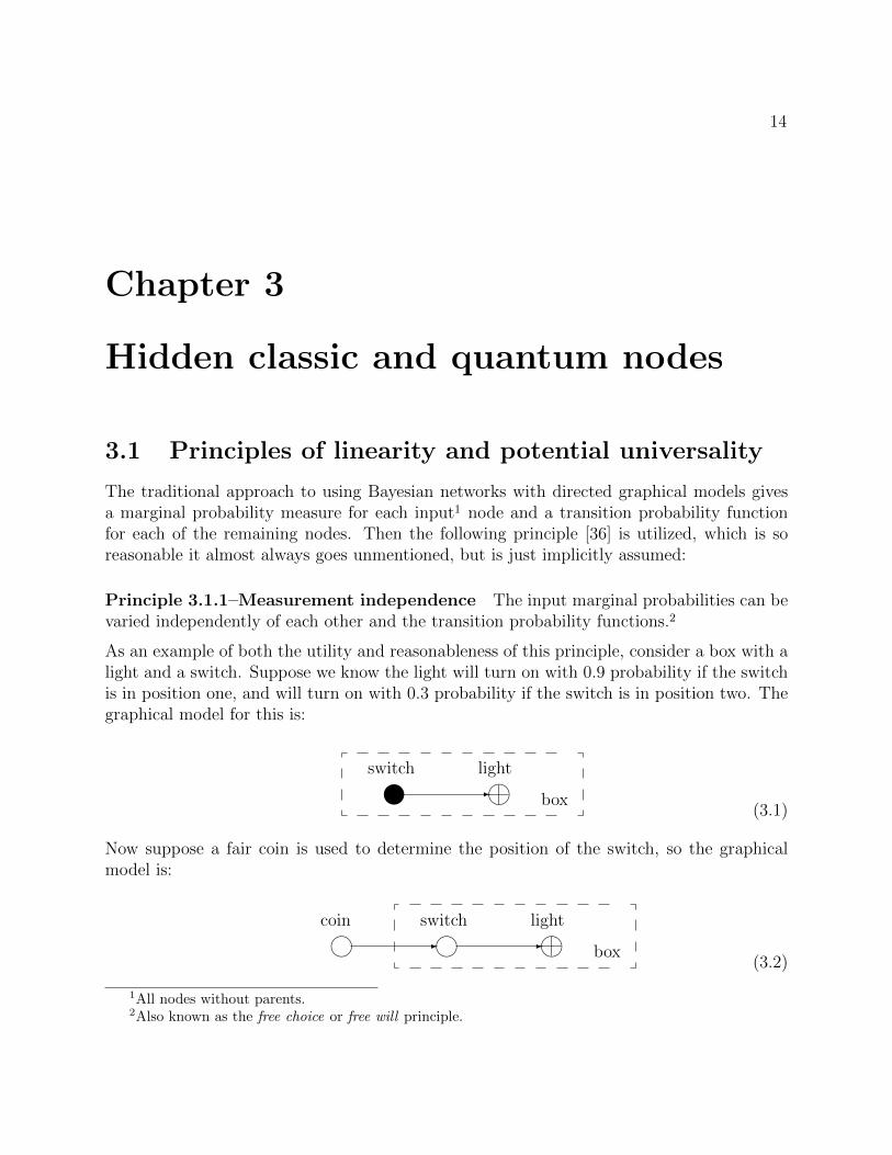
As an example of both the utility and reasonableness of this principle, consider a box with alight and a switch. Suppose we know the light will turn on with 0.9 probability if the switchis in position one, and will turn on with 0.3 probability if the switch is in position two. Thegraphical model for this is:
mswitch light
box-
(3.1)
Now suppose a fair coin is used to determine the position of the switch, so the graphicalmodel is:
m m mcoin switch light
box- -
(3.2)
1All nodes without parents.2Also known as the free choice or free will principle.
CHAPTER 3. HIDDEN CLASSIC AND QUANTUM NODES 15
Using the preceding principle, then there is a 0.5 ⋅0.9+0.5 ⋅0.3 = 0.6 probability the light willturn on. Without this principle or something similar, it would be impossible to predict thebehavior of the light using the coin to determine the switch position just using our knowledgeabout what would happen with each position of the switch.
From the metaphysical viewpoint this principle makes perfect sense. If there are actuallyexisting variables that take actual values (such as the position of the switch), observedoutcomes depend only these and not on probability measures, which are only a reflection ofour ignorance. As has already been commented on, this justification fails for hidden nodes,which are hypothetical constructs we introduce. Without this metaphysical backing, theprinciple is actually far stronger than what is required in that it assumes the existence oftransition probability functions.
If the principle is assumed true, then, from (2.14), the calculation of the joint probabilityreduces to some combination of composition and tensor product of of linear maps, involvingboth those induced by the given transition probability functions, restriction maps, and pos-sibly the Copy map (the last two of which are also induced by certain transition probabilityfunctions–see §2.5). By A3.2 and A3.3, this calculation is well-defined. For instance, thecalculation of the joint probability for (2.20), with θ(⋅∣⋅) and ζ(⋅∣⋅) as transition probabilityfunctions, can be given as3,4
(RA K ((RB L)⊗ I) Copy RCν)(X ) (3.3)
for L the map induced by θ(⋅∣⋅), K the map induced by ζ(⋅∣⋅), I the identity map on measures,and RA, RB, RC restriction maps. By introducing an initializing map, Li, on the trivialmeasure space5, which is isomorphic to R, with constant value µ and a terminal map, Lt,which evaluates the measure on X (hence, is a map to the trivial measure space), this canbe written purely in terms of maps:
Lt RA K ((RB L)⊗ I) Copy RC Li (3.4)
Later, we will introduce hidden nodes of a special form to account for initializing or termi-nating maps (see §4.1).
Therefore, the joint probability is a multilinear functional on the input marginal prob-abilities. Furthermore, by a convergence theorem for sequences of measures [56], it is notjust linear for finite linear combinations in each marginal measure, but absolutely convergentcountable linear combinations as well. Hence, for any one input node, if Φ is the functional
3We adopt the usual mathematical convention of maps acting on the left. The opposite convention ofmaps acting on the right is also commonly employed in the literature for the classical observed case [47].
4We will follow the convention that the tensor product of vector spaces consists of all finite linearcombinations (the algebraic tensor product) except if both are Hilbert spaces, in which case it is the Hilbertspace given by the completion using the standard induced inner-product. The tensor product K⊗L of linearmaps L ∶ A→ C and K ∶ B→ D is, for closed, linear spaces E ⊂ A⊗B and F ⊂ C⊗ F, the set of all linear mapsM ∶ E → F which, when restricted to A⊗ B, agree with K ⊗ L. If this set consists of a single map, K ⊗ L istermed well-defined.
5A measure on a set X is trivial if the only subsets in its σ-algebra are ∅,X.
CHAPTER 3. HIDDEN CLASSIC AND QUANTUM NODES 16
(with all the marginal probability measures for other nodes fixed) and ⟨µj⟩ is a sequence ofmarginal probability measures for that node with ∑j ∥µj∥ finite, then Φ (∑j µj) = ∑j Φµj. Itis obvious that it would still be possible to make the calculation for the above example withthe box based simply on this linearity property, which is weaker than the above property.
As we have already mentioned, we will consider hidden nodes associated to maps onspaces other than the space of measures. Therefore, we introduce the following weaker andmore general version of the above principle:
Principle 3.1.2–Linearity The maps for a Bayesian network are linear and bounded(hence, continuous).
Moreover, we want the maps for graph fragments to be universal in the sense that themodules (such as the box in the preceding example) can be used to make predictions in novelsituations. While this may fail in practice, this should be as a result of experiment and notbe preordained by the mathematical models employed. We insist, therefore, on potentialuniversality in the sense that any possible tensor product (not just those for a particularnetwork) of the linear maps employed should always be well-defined.
Principle 3.1.3–Potential universality The space of linear maps employed must besuch that any tensor product of maps in the space is well-defined.
The repercussions of the latter two principles will be studied in the following.
3.2 Options I and II
A problem arising from potential universality
Generalizing from maps induced by transition probability functions to more general linearmaps, composition is not an issue. However, the principle of potential universality does nothold in general for maps on measures on specified sets for specified σ-algebras of events. Oneproblem is the lack of uniqueness. Suppose one has the identity map I on Borel6 measureson the interval [0,1] with the usual topology. Define I⊗I to be the set of all bounded, linearmaps L on the Borel measures on [0,1] × [0,1], with the usual product topology, such that,restricted to product measures, µ×ν, L(µ×ν) = (Iµ)× (Iν) = µ×ν. One obvious member ofI⊗I is simply the identity map on the Borel measures on [0,1]×[0,1]. This is the only weak*-continuous7 map in the set. Another map in the set is given by K ∶ ρ→ ⋁(ρ ∥ (µ×ν)), where
6The Borel σ-algebra on a topological space is that generated by the open subsets.7Using the Riesz theorem [57] which states that Radon (defined in the following) measures on a compact
set are dual to the continuous functions on that set. A measure on a topological space is inner regular ifthe measure of any set is approximated by the measure of compact sets it contains. It is outer regular if themeasure of any set is approximated by the open sets that contain it. A measure is Radon if it is Borel and
CHAPTER 3. HIDDEN CLASSIC AND QUANTUM NODES 17
the supremum is taken over all product measures and ρ ∥ (µ × ν) is the part of ρ absolutelycontinuous with respect to µ × ν using Lebesgue decomposition [55]. This is a well-definedmap by B2.1 that differs from the identity map. For instance, let ρ be the diagonal Lebesguemeasure,
ρ(A) = λ (a ∈ [0,1]∣(a, a) ∈ A) (3.5)
Then the identity map sends ρ to itself, whereas Kρ = 0.Another possible problem is the lack of existence. Not every linear map can be extended.
For example, the space of sequences with limit zero, c0, is a norm-closed8, weak*-dense9
subset of the bounded sequences, `∞. However, there is no extension of the identity mapc0 → c0 to a projection `∞ → c0. [3] [90] However, it is not clear whether there is a similarproblem with extending the tensor product of linear maps.
Resolving the problem–two options
There are various ways to resolve this dilemma. One is to revert to only considering linearmaps induced by transition probability functions, which works by A3.3. We will not pursuethis approach since it has no ready generalization to linear maps on spaces other than thoseof measures. Instead, we will consider two approaches which do. The first, which will betermed option I, is to limit the space of measures so as to eliminate measures such as ρabove. The alternative, which will be termed option II, is to impose additional structure onthe sets and then to limit the space of maps, so as to eliminate maps such as K above.
To implement option I, a basic property that we want for our subsets of measures isdefined by:
Definition 3.2.1 A subset A of measures is absolutely-continuous-complete if, for any µin A, all measures absolutely continuous with respect to µ are also in A.
By the Radon-Nikodym theorem and the density of simple functions10 in L1-spaces, a subsetof finite measures A will have this property if, given any measure µ ∈ A, all the restrictions µ∣Eover µ-measurable subsets E are also in A. Hence, this property is the minimal requirementto show that a map is indeed positive. Then from A1.2, A1.3, B1.3, B1.4, and B2.5, thenecessary and sufficient condition to implement option I is that the tensor product of thesubsets of measures for each set is norm-dense11 in the subset of measures for the productset.
inner regular. If the space is compact and Hausdorff, and the measure is finite, then it is also necessarilyouter regular. If the space is compact, Hausdorff, metric, and separable, then Borel measures are necessarilyRadon [58].
8Using the supremum norm.9Using the duality of `1 and `∞.
10A simple function takes on only finitely many values.11Using the total-variation norm.

CHAPTER 3. HIDDEN CLASSIC AND QUANTUM NODES 18
A sufficient method, termed option I’, to insure this is met is for each set to have anassociated base measure. The base measure need not be finite, but it must be σ-finite. Thenthe associated subset of measures is the set of all finite measures absolutely continuous withrespect to the base measure, which by the Radon-Nikodym theorem is equivalent to the spaceof L1-functions with respect to the base measure. The base measure for the direct productof sets must be the product of the base measures for the individual sets. The sufficiency ofthis prescription is given by B3.1.
Another sufficient method is to instead use the space of atomic measures12. If there areuncountably many atoms in the σ-algebra, this is distinct from option I’; otherwise, thecounting measure that assigns one to each atom is a base measure. The sufficiency of thisprescription is given by B6.1 and B6.2. It is also possible to combine these two sufficientapproaches, say by using the atomic, L1(X ;µ)-valued vector E-measures on Y. This issufficient by B3.1, B6.1, and B6.2.
The implementation of option II is more straightforward. Each set has a topologicalstructure that makes it a compact, Hausdorff space. By Tychonoff’s theorem [42] [59], thedirect product of compact spaces with the product topology is necessarily compact. All theσ-algebras are required to be the Borel σ-algebra. The linear maps are restricted to thosethat are weak* continuous; in other words, those maps that are the adjoints to linear mapson continuous functions going in the opposite direction. In practice, rather that working withthe adjoint maps, one works with the linear maps in the opposite direction. The propositionsA1.3, C1.1, and C2.4 gives the sufficiency of this prescription.
Comments on the two options
For option I’, the need for base measures is not generally a troublesome issue. For σ-algebrasgenerated by a countable number of atomic subsets13, the counting measure that assigns oneto each atom is a base measure for any finite measure. For classical physics, with configura-tion space X and phase-space given by the cotangent bundle T ∗X , the symplectic phase-spacevolume-form14 Ω provides a natural base measure, since by Heisenberg’s uncertainty princi-ple, not even all measures absolutely-continuous with respect to Ω are accessible, let alonemore singular measures.
Note that allowing the base measure to be a σ-finite measure is only for purposes ofconvenience in allowing the commonly employed Lebesgue measure on unbounded subsetsof Rn, as the following theorem shows:
Theorem 3.2.2 Given any σ-finite measure µ on a set X , there is a finite measure ν suchthat L1(X ;µ) is isometric to L1(X ;ν), where the isomorphism is a pointwise scaling.
12A measure is atomic if there is a union of countably many atoms in the σ-algebra such that thecomplement of the union has measure zero.
13A subset in a σ-algebra is atomic if it is indivisible in the σ-algebra.14As a measure, locally Ω is simply Lebesgue measure with respect to any canonical choice of local position
and momentum coordinates.

CHAPTER 3. HIDDEN CLASSIC AND QUANTUM NODES 19
Proof If µ is finite, there is nothing to show, so assume it is not. Since µ is σ-finite, there isa countable collection of disjoint subsets Bj of X such that µ(Bj) is finite and nonzero for
each j ∈ 1,2, . . . and ⋃∞j=1Bj = X . Then let the finite measure ν be given by ν∣Bj =
µ∣Bj2jµ(Bj)
.
◻
However, there are two complaints with option I’. One is that for σ-algebras not gener-ated by a countable number of atomic subsets, there is no Copy map; hence, except for this(effectively discrete) case, hidden nodes either have only one child node or are terminated.The second complaint is that passing a continuously variable parameter to a hidden nodeas a simple number is not permitted (unless that particular value corresponds to an atomin the base measure); instead, one must use a sharply peaked measure. This adds signifi-cant complexity for little gain in cases where one is not especially interested in modellinguncertainty in the inputs (see §4.5 and §8.2 for instances).
For option II, the restriction to topological spaces and Borel σ-algebras is also not trou-blesome, since these are typically used in any case. The limitation of using compact spacesappears severe, but locally compact spaces15 can also be used with the restriction that themaps take continuous functions vanishing at infinity to continuous functions vanishing atinfinity, so the adjoint maps on measures do not “leak away” measure at infinity.
In addition, for option II, the first complaint above does not occur since the Copy map isadjoint to the map Copy∗ that takes continuous functions on X ×X to continuous functionson X by (Copy∗f)(x) = f(x,x) (which can obviously be generalized to make any finitenumber of copies). The second complaint does not occur either since the evaluation map iswell-defined for continuous functions. However, there is now the opposite problem in that wewish to calculate probabilities on sets, so we need maps on characteristic functions, not justcontinuous ones. One solution is to extend each map to one from bounded, Borel measurablefunctions to bounded, Borel measurable functions; by C2.9 this can always be done in aunique manner. Another solution is to use the results on continuous functions to get theresult for characteristic functions of open sets as in the proof of the Riesz theorem [57]; thenouter regularity gives the result on any characteristic function of a Borel set.
Note that for option I’, the considered linear map L ∶ L1(X ;µ) → L1(Y;ν) is alwaysinduced by an object τ(⋅∣⋅) which is given by, for ν-measurable sets B, τ(B∣⋅) = L∗1B (whichis of course actually an equivalence class of functions that agree almost everywhere withrespect to µ) with the adjoint map L∗ ∶ L∞(Y ;ν)→ L∞(X ;µ):
∫y∈B
(Lf)(y)dν(y) = ∫y∈Y
1B(Lf)(y)dν(y) = ∫x∈X
f(x)(L∗1B)(x)dµ(x) (3.6)
= ∫x∈X
f(x)τ(B∣x)dµ(x)
15A space is locally compact if it can be compactified by the addition of one point, the point-at-infinity. [43]. [60]

CHAPTER 3. HIDDEN CLASSIC AND QUANTUM NODES 20
for any f ∈ L1(X ;µ). It is not clear whether it is possible to select a particular functionfrom each equivalence class consistently to get a transition probability function. Similarly,if we use option I with the measures limited to the atomic measures, the considered linearmap L ∶ A(X ;E) → A(Y;F) is always induced by an object τ(⋅∣⋅) which is given by, for setsB ∈ F , τ(B∣x) = (LδA)(B) for x in the atomic set A ∈ E :
(Lµ)(B) = ∫x∈X
τ(B∣x)dµ(x) (3.7)
for any atomic measure µ ∈ A(X ;E). However, in general τ(⋅∣⋅) will not be a transitionprobability function since there is no reason for τ(B∣⋅) to necessarily be E-measurable. Also,for option II, by C2.8, for the considered linear map L ∶ C(Y) → C(X ), the adjoint mapL∗ ∶M(X )→M(Y) is induced by the transition probability function τ(⋅∣⋅) given by τ(B∣x) =(Lδx)(B) for any x ∈ X and Borel subset B ⊂ Y:
(L∗µ)(B) = ∫x∈X
τ(B∣x)dµ(x) (3.8)
for any Radon measure µ ∈ M(X ). However, it is more fruitful to consider the mapsthemselves as the primary objects of interest rather than the transition probability functionsor the similar objects. As is shown in the following section, the maps can be generalized tobe maps on structures other than measures, whereas the transition probability functions orsimilar objects do not.
3.3 Quantum nodes
Expanding the space of considered maps
As an alternative to linear maps on measures, consider linear maps on density matrices16,17
or, more generally, density matrix-valued measures. We will show below that, with somerestrictions on the maps, this can be made to work consistently with the propositions givenin §3.1. We will show in §5.1 that this gives rise to models that are consistent with theusual, textbook quantum mechanics; therefore, nodes whose linear maps involve densitymatrices will be termed quantum. However, the term quantum should not be taken to implythese maps are necessarily only of utility in situations traditionally thought of as in the
16A Hilbert space will be taken to be any complete, sesquilinear inner-product space, without regard tocardinality of dimension or separability. The density matrices D(H)+ will be taken to be the self-adjoint,positive operators on a given Hilbert space H.
17A linear map from D(H) to D(J) is commonly referred to as a superoperator in the literature. We choosenot to employ this terminology for the following reasons: (i) linear maps is already standard mathematicalterminology and is in common use in the analogous classical situation, for instance Markov maps; (ii)superoperator seems to imply a map on all bounded operators, B(H), when in general it is not possible toextend the domain of the map beyond the trace-class operators, S1(H); and (iii) the use of super- risksconfusion with the unrelated supersymmetry and superstrings.

CHAPTER 3. HIDDEN CLASSIC AND QUANTUM NODES 21
domain of quantum mechanics–in principle, any hidden node in any forecasting situation,say forecasting weather or stock prices, could be a quantum node. It is up to experiment todetermine if these are of utility. Thus far, we are unaware of any structures besides measuresand density matrices that have the requisite properties to be employed in modelling. Thequestion of whether or not there are such additional structures will be further explored in§3.8 below.
Following our work in the preceding section, for option I, instead of linear maps on subsetsof real-valued measures, we have linear maps on subsets of the D(H)+-valued vector measures.For option I’, we will require the vector measures to be absolutely continuous with respectto a base measure. Since D(H) has the Radon-Nikodym property [14], this is equivalent tohaving D(H)+-valued, Bochner-integrable functions. The constraint of potential universalitymandates having well-defined tensor product of maps; this is maintained by A1.3 and B4.1if the tensor product is bounded.
Similarly to the classical case, another sufficient approach to implementing option I is totake the atomic, D(H)+-valued vector measures, as is shown by B6.1 and B6.2. It is alsopossible to combine these two sufficient approaches, say by using the atomic, L1(X ;µ;D(H))-valued vector E-measures on Y. This is sufficient by B4.1, B6.1, and B6.2.
For option II, instead of maps on real-valued, positive, continuous functions, one has mapson continuous functions that take values in the self-adjoint, positive, compact18 operators ona Hilbert space H, K(H)+. Self-adjoint, compact operators are used since they are the predualto the self-adjoint trace-class operators. [50] Once again, potential universality mandateshaving well-defined tensor products of maps; as before, this is maintained if the tensorproduct is bounded, now by A1.3 and C3.1.
Problem arising from positivity and potential universality
Of course, everything is not really that simple. The tensor product of bounded maps maynot be bounded. Also, even if both maps are positive, their tensor product need not be.To illustrate these problems, take a separable, infinite-dimensional Hilbert space H, fix someorthonormal basis ej, and consider the transpose map T relative to that basis:
T⎛⎝∑j,k
ajkej ⊗ e∗k⎞⎠=∑j,k
akjej ⊗ e∗k (3.9)
where e∗k is the functional ⟨⋅,ek⟩. This is well-defined on the space of density-matrices onH, D(H)+, since, by the spectral theorem for compact operators [17], any such operatorcan be written in the form of an infinite matrix with finite rank operators correspondingto truncated matrices converging in trace norm. (Of course, since density-matrices are self-adjoint, T could also be termed the conjugate map relative to the basis). This map is clearlypositive and has operator norm one.
18An operator is compact if the image of any bounded sequence has a convergent subsequence.

CHAPTER 3. HIDDEN CLASSIC AND QUANTUM NODES 22
However, consider the tensor product map T⊗IMn acting on density matrices D(H⊗Cn)+,where IMn is the identity map acting on n × n-matrices. For the rank-one operator ψ ⊗ ψ∗with
ψ =n−1
∑j=0
e(n+1)j+1 (3.10)
we have (T ⊗ IMn)(ψ ⊗ ψ∗) = S. Truncating S to the span of e1, . . . ,en2 (it is zeroelsewhere), it is the matrix form of the transpose map acting on Mn written in vector form
using the Vec operation19. Therefore, S clearly has eigenvalue one with multiplicity n(n+1)2
and eigenvalue minus one with multiplicity n(n−1)2 . Hence, T ⊗ IMn is not positive, and
∥T ⊗ IMn∥op ≥1
∥ψ∥2(n(n + 1)
2∣1∣ + n(n − 1)
2∣ − 1∣) = n
2
n= n (3.11)
By [19], ∥T ⊗ IMn∥op = n and this example is maximal. This is clearly unbounded as n→∞.
Solution to the problem
The solution to both the positivity and the boundedness problem is to require complete-positivity for the maps. This has several definitions (see B2.6, B5.6, C2.1) that are equiv-alent (see B5.8, C5.6); the basic notion is that all tensor products with various identitymaps should be positive. Since the composition of positive maps is positive, this immediatelyimplies that complete-positivity is preserved under both composition and tensor products.Furthermore, from B2.5, B2.5, C2.4, and C5.3, the operator norm is a cross-norm20 forcompletely-positive maps, so this resolves the boundedness problem as well. The completely-positive maps clearly form a convex cone within the space of all maps; this cone is closed inthe norm topology and in various weaker topologies by B5.12, B5.14, and C5.10; however,unlike the cone of positive maps, in infinite dimensions it has no interior in any of thesetopologies, which raises issues for approximation in numerical calculation.
3.4 No quantum copying
It is commonly stated that cloning is something that is possible classically, but is impossiblein quantum mechanics. This is based on false analogy. The correct situation is that thereare two different notions, that of copying and that of cloning, that are being confused. Once
19Vec takes a n × n-matrix to a column vector of height n2 by stacking columns.20A norm is a cross-norm if ∥a ⊗ b∥ ≤ ∥a∥∥b∥. Note the property of being a cross-norm depends on the
choice of norms for the individual spaces as well as for the larger space containing the tensor products.
CHAPTER 3. HIDDEN CLASSIC AND QUANTUM NODES 23
these two have been separated, we have the following situation:
classical quantum
copyingExists and implementablesince linear.
Does not exist.
cloning
Exists but not imple-mentable since neitherlinear nor the ratio of linearmaps.
Exists but not imple-mentable since neitherlinear nor the ratio of linearmaps.
The confusion is comparing the upper left and lower right entries instead of correctly goingacross. Cloning is possible for neither classical nor quantum Bayesian networks (as will beshown below in §6.1) for exactly the same reason, so it does not differentiate the two. On theother hand, copying is possible classically (except for issues arising from potential universalityconsidered above in §3.2), but cannot even be defined as a mathematical operation on densitymatrices.
Classical copying
As has already been mentioned (see §2.5), there is a Copy map from measures on a set Xto measures on X ×X . When X is a compact set, this map is weak*-continuous, being theadjoint of the previously discussed map (Copy∗f)(x) = f(x,x). The Clone map is given byµ→ µ×µ. For the single atom measure for atom C, where for any measurable subset A ⊂ X ,
δC(A) =⎧⎪⎪⎨⎪⎪⎩
1 if A ⊃ C0 otherwise
(3.12)
we haveCopy δC = δC × δC = Clone δC (3.13)
This is likely the source of confusion between the Copy and Clone maps for the classicalcase.
Instead of using this explicit form for Copy, an approach that will prove useful in thequantum case is to start with some basic properties, then find the implications. One propertyof what is commonly accepted as the notion of a copy is that the probability for both copiesto have a specified property is equal to that for each copy to have it, which is equal to thatof the original having it, so for any unit-norm measure µ on X and any µ-measurable setA ⊂ X ,
Property C Copy µ(A ×A) = Copy µ(A ×X ) = Copy µ(X ×A) = µ(A)
Note this property implies Copy µ(A × (X ∖ A))) = Copy µ((X ∖ A) × A) = 0. Now givena σ-algebra E of subsets of X , let F be the σ-algebra generated by the rectangular subsetsE × E . Then we have the following:

CHAPTER 3. HIDDEN CLASSIC AND QUANTUM NODES 24
Theorem 3.4.1 Any map L from unit-norm E-measures on X to unit-norm F -measureson X ×X obeying property C is linear for convex linear combinations.
Comment Since any finite measure can be scaled to have unit-norm, this implies themap can be extended to all finite measures, with the extended map being positively linear.By the generating property of measures among signed measures as a result of Jordan de-composition [61], this implies the map can further be extended to a linear map on signedmeasures.
Proof Let L be such a map and µ an unit-norm E-measure on X . For any subsets A,B ∈ E ,by the properties of measures,
(Lµ)(A ×B) =(Lµ)((A ∩B) × (A ∩B)) + (Lµ)((A ∩B) × (B ∖ (A ∩B))) (3.14)
+ (Lµ)((A ∖B) ×B)
However, (A∩B)× (B ∖ (A∩B)) ⊂ (A∩B)× (X ∖ (A∩B)) and (A∖B)×B ⊂ (X ∖B)×B,so, by property C and its implication,
(Lµ)(A ×B) = (Lµ)((A ∩B) × (A ∩B)) = µ(A ∩B) = (Lµ)(B ×A) (3.15)
Let ρ be another unit-norm E-measure on X . Then for any t ∈ [0,1], (1− t)ρ+ tµ will bea unit-norm E-measure on X . Consider the signed measure on X ×X given by
νt = L((1 − t)ρ + tµ) − (1 − t)Lρ − tLµ (3.16)
Take any A ∈ E . Then, by property C, νt(A × A) = 0. However, by the above symmetryproperty of L,
νt(A ×B) = 1
2(νt(A ×B) + νt(B ×A)) (3.17)
which is equal to
12 (νt((A ∪B) × (A ∪B)) − νt((A ∖B) × (A ∖B)) (3.18)
−νt((B ∖A) × (B ∖A)) + νt((A ∩B) × (A ∩B)))
which is zero by the preceding property of νt. Since A,B were arbitrary, νt must be the zeromeasure. ◻
Quantum Copying
The Clone map taking a density matrix on the Hilbert space H to one on H ⊗ H is definedas ρ → ρ⊗ ρ. How to define a Copy map is not obvious. By analogy to the classical case, itshould have the following properties for any unit-trace density matrix ρ and any projectorE:
CHAPTER 3. HIDDEN CLASSIC AND QUANTUM NODES 25
Property Q tr (E ⊗E) Copy ρ = tr (E ⊗ IH) Copy ρ = tr (IH ⊗E) Copy ρ = tr Eρ
Note this implies tr (E ⊗ (IH − E)) Copy ρ = tr ((IH − E) ⊗ E) Copy ρ = 0. Then we havethe following:
Theorem 3.4.2 Any map L from unit-trace density matrices on H to unit-trace densitymatrices on H⊗H obeying property Q is linear for convex linear combinations.
Comment Since any density matrix can be scaled to have trace one, this implies the mapcan be extended to all density matrices with the extended map being positively linear. Bythe generating property of density matrices among signed density matrices as a result of thespectral theorem for compact operators, this implies the map can further be extended to alinear map.
Proof Let L be such a map and ρ an unit-trace density matrix on H. For any commutingprojectors E, F,
tr (E ⊗ F )(Lρ) =tr (EF ⊗EF )(Lρ) (3.19)
+ tr (EF ⊗ (F −EF ))(Lρ) + tr ((E −EF )⊗ F )(Lρ)
However, by positivity and the implication of Q,
0 ≤ tr (EF ⊗ (F −EF ))(Lρ) ≤ tr (EF ⊗ (IH −EF ))(Lρ) = 0 (3.20)
and0 ≤ tr ((E −EF )⊗ F )(Lρ) ≤ tr ((IH − F )⊗ F )(Lρ) = 0 (3.21)
so, using Q,
tr (E ⊗ F )(Lρ) = tr (EF ⊗EF )(Lρ) = tr EFρ = tr (F ⊗E)(Lρ) (3.22)
Let τ be another unit-trace density matrix on H. Then for any t ∈ [0,1], (1− t)ρ+ tτ willbe a unit-trace density matrix on H. Consider the signed density matrix on H⊗H given by
νt = L((1 − t)ρ + tτ) − (1 − t)Lρ − tLτ (3.23)
Take any projector E. Then, by property Q, tr (E ⊗ E)νt = 0. However, by the abovesymmetry property of L, for any commuting projectors E, F,
tr (E ⊗ F )νt =1
2(tr (E ⊗ F )νt + tr (F ⊗E)νt) (3.24)
which is equal to
1
2(tr ((E + F −EF )⊗ (E + F −EF ))νt − tr ((E −EF )⊗ (E −EF ))νt (3.25)
−tr ((F −EF )⊗ (F −EF ))νt + tr (EF ⊗EF )νt)

CHAPTER 3. HIDDEN CLASSIC AND QUANTUM NODES 26
which is zero by the preceding property of νt. Since E,F were arbitrary, νt must be the zerooperator. ◻We then have the following theorem, based on the argument of Wooters and Zurek [92] thatdensity matrices of rank greater than one can be expressed in more than one way (infinitelymany ways actually) to create a contradiction.
Theorem 3.4.3 There is no quantum Copy map for non-trivial21 H.
Proof Take any orthonormal u,v ⊂ H with corresponding adjoint operators u∗ = ⟨⋅,u⟩Hand v∗ = ⟨⋅,v⟩H. Consider ρ = 1
2 (u⊗ u∗ + v ⊗ v∗). By linearity,
Copy ρ = 1
2( Copy (u⊗ u∗) + Copy (v ⊗ v∗)) (3.26)
By property Q, for rank one density matrices Copy must be the same as Clone, so Copy ρis uniquely given as
1
2(u⊗ u⊗ u∗ ⊗ u∗ + v ⊗ v ⊗ v∗ ⊗ v∗) (3.27)
However, it is also possible to write ρ as
1
4((u + v)⊗ (u + v)∗ + (u − v)⊗ (u − v)∗) (3.28)
Then Copy ρ is uniquely given as
1
8((u + v)⊗ (u + v)⊗ (u + v)∗ ⊗ (u + v)∗ (3.29)
+(u − v)⊗ (u − v)⊗ (u − v)∗ ⊗ (u − v)∗)
= 1
4(u⊗ u⊗ u∗ ⊗ u∗ + u⊗ u⊗ v∗ ⊗ v∗ + u⊗ v ⊗ u∗ ⊗ v∗
+ u⊗ v ⊗ v∗ ⊗ u∗ + v ⊗ u⊗ u∗ ⊗ v∗ + v ⊗ u⊗ v∗ ⊗ u∗++v ⊗ v ⊗ u∗ ⊗ u∗ + v ⊗ v ⊗ v∗ ⊗ v∗) (3.30)
Clearly, (3.27) and (3.30) are unequal, which is a contradiction. ◻
3.5 Embedding quantum models into classical ones
A construction for option I’ using atomic measures
For option I’, there is a way to embed quantum behavior into a purely classical, but contex-tual, model. For any Hilbert space H, let SH be the closed unit ball within H. Let SH/ ∼ be
21A trivial Hilbert space has dimension one.
CHAPTER 3. HIDDEN CLASSIC AND QUANTUM NODES 27
the quotient set formed from SH by the equivalence relation ψ ∼ ξ if there is a phase22 w suchthat ψ = wξ. Clearly SH/ ∼ is in one-to-one correspondence to rank-one projectors on H. LetE be any σ-algebra on SH/ ∼ such that all points are atoms (such as the Borel σ-algebra).For any set X and base measure µ denote the space of atomic, finite-norm, L1(X ;µ)-valuedvector E-measures on SH/ ∼ by A (SH/ ∼;E ;L1(X ;µ)). This is a Banach space by B6.1.Given τ ∈ A (SH/ ∼;E ;L1(X ;µ)), for any µ-measurable subset B ⊂ X , define τB to be theatomic, signed E-measure on SH/ ∼ defined by τB(A) = ∫B τ(A)dµ for any A ∈ E . Let ∼′ bethe equivalence relation on A (SH/ ∼;E ;L1(X ;µ)) given by τ ∼′ χ if, for any µ-measurablesubset B ⊂ X ,
∫s∈SH/∼
ss∗ dτB(s) = ∫s∈SH/∼
ss∗ dχB(s) (3.31)
Since the equivalence class using ∼′ of zero is a closed, linear subspace, the quotient spaceA (SH/ ∼;E ;L1(X ;µ)) / ∼′ is a Banach space using the standard norm for quotient spaces,∥[τ]∥ = infχ∈[τ] ∥χ∥. Define the positive cone on the quotient space to be those equivalenceclasses with a positive member, using the obvious notion of positivity onA (SH/ ∼;E ;L1(X ;µ)).
Then we have the following theorem:
Theorem 3.5.1 There is a positive, linear, isometric isomorphism,
L1 (X ;µ;D(H)) ≅ A (SH/ ∼;E ;L1(X ;µ)) / ∼′
Proof If the measure µ is trivial, then L1 (X ;µ;D(H)) ≅ D(H). Define the map Ψ ∶L1 (X ;µ;D(H))→ A (SH/ ∼;E ;L1(X ;µ)) / ∼′ by Ψ(ρ) being the equivalence class of ∑j ajδ[ψj]for ρ = ∑j ajψjψ
∗j with countable collections ψj ∈ SH and aj ⊂ R, which is always possible
by the spectral theorem for compact operators.For more general measures on X , first start with the observation that, given any ρ ∈
L1 (X ;µ;D(H)), each ρ(x) lives in the same separable subspace of H for almost every x withrespect to µ, namely the subspace G that the operator ∫x∈X ∣ρ(x)∣dµ ∈ D(H) lives in. Letej be an orthonormal basis for G. For each j ∈ 1,2, . . ., let Pj be the orthogonal projectoronto the span of e1,e2, . . . ,ej. Since simple functions are norm-dense in L1 (X ;µ;D(H)),the sequence ⟨PjρPj⟩ is a Cauchy sequence by C4.3; hence, it converges in norm by thecompleteness of the Banach space L1 (X ;µ;D(H)). It is readily seen that the limit pointis ρ. Now define the map Ψ ∶ L1 (X ;µ;D(H)) → A (SH/ ∼;E ;L1(X ;µ)) / ∼′ by first definingΨ(ψψ∗f), for ψ ∈ H and f ∈ L1(X ;µ) to be the equivalence class of the vector measuref ⊗ δ[ψ]. Since the linear space D(PmH) is spanned by the m2 operators
eje∗j j∈1,...,m ∪ (ej + ek)(ej + ek)∗, (ej + ıek)(ej + ıek)∗j,k∈1,...,m,j<k (3.32)
the map Ψ can be extended by linearity to all ρ with the property that ρ(x) lives on thesame finite-dimensional subspace of H for almost every x with respect to µ.
22Elements of C with magnitude one.
CHAPTER 3. HIDDEN CLASSIC AND QUANTUM NODES 28
Now take any ρ with this property which is also a simple function. Then, applying the(finite-dimensional) spectral theorem to each of the finitely many values ρ takes, Ψ is readilyseen to be a positive isometry. Since simple functions are norm-dense, by A1.2, Ψ is apositive isometry on all ρ with the property that ρ(x) lives on the same finite-dimensionalsubspace of H for almost every x with respect to µ. However, by an above argument, such ρare norm-dense in L1 (X ;µ;D(H)). Hence, using A1.3 to extend Ψ to all of L1 (X ;µ;D(H)),Ψ is a positive isometry. It remains to show it is surjective, but that is easily seen, with
Ψ−1 ([∑j
fj ⊗ δ[ψj]]) =∑j
fjψjψ∗j (3.33)
for any ∑j fj ⊗ δ[ψj] ∈ A (SH/ ∼;E ;L1(X ;µ)). ◻
Comment Since SH×SJ ≇ SH⊗J if neither H nor J are trivial, this construction is necessarilycontextual. Therefore, it does not violate Bells’ inequality (see §6.3 below).
The nonexistence of the corresponding construction using a basemeasure
The corresponding construction using a base measure ν would be for there to be a positiveisometry from L1(X ;µ;D(H)) to a quotient space of some L1(Y;ν). This is impossible, asthe following theorem shows:
Theorem 3.5.2 If the Hilbert space H is non-trivial, there are no: (i) set Y; (ii) σ-finitemeasure ν; and (iii) equivalence relation ∼ induced by a closed, linear subspace B ⊂ L1(Y;ν)–such that there is a positive, linear isomorphism, Ψ ∶ L1 (X ;µ;D(H)) → L1(Y;ν)/ ∼, whichis also an isometry on the positive cone.
Proof Suppose otherwise. Then there is a L1 (X ;µ;D(H))-valued vector measure τ on Yprovided by τ(A) = Ψ−1 ([1A]) for any ν-measurable subset A ⊂ Y. The spaces L1(Y;ν)∗ ≅L∞(Y;ν) by Riesz’s theorem [62]. The dual to L1(Y;ν)/ ∼ is provided by the annihilator B⊥:the closed, linear subspace of L∞(Y;ν) that annihilates B. (Note, in particular that since Ψis an isometry on the positive cone, the constant function 1Y ∈ B⊥.) Therefore, there is anadjoint map Ψ∗ ∶ B⊥ → L1 (X ;µ;D(H))∗ given by
∫Yf Ψρdν = (Ψ∗f)ρ (3.34)
for any f ∈ B⊥ and ρ ∈ L1 (X ;µ;D(H)). By the basic properties of Banach spaces, (Ψ∗)−1 =(Ψ−1)∗, Ψ∗ is positive, and Ψ∗ is an isometry on the positive cone.
Then,
∫A
Ψ∗−1Φdν = Φ(τ(A)) (3.35)

CHAPTER 3. HIDDEN CLASSIC AND QUANTUM NODES 29
for any linear functional Φ ∈ L1 (X ;µ;D(H))∗ and ν-measurable subset A ⊂ Y. For IH theidentity operator, Ψ∗−1 (IH1X ) is the element of B⊥ that agrees with the norm when integratedwith any positive function in L1(Y;ν)/ ∼; hence, it must be 1Y . Therefore,
∫X
tr τ(A)dµ = ∫A
Ψ∗−1 (IH1X ) dν = ν(A) (3.36)
However, this gives rise to a contradiction. Fix some subset B ⊂ X with 0 < µ(B) < ∞.Take any unit norm ψ ∈ H. Since Ψ is positive, by definition, the equivalence class Ψ(ψψ∗1B)has a positive member, call it gψ. There must be some ψ ≠ ξ such that A = gψ > 0∩gξ > 0has strictly positive ν-measure; otherwise, there would be an uncountable collection gψ > 0indexed by unit norm ψ ∈ H of subsets of Y, each with strictly positive ν measure, but whosepairwise intersections all have ν-measure zero. The existence of such a collection wouldcontradict ν being σ-finite by B1.6. Since Ψ is an isometry on the positive cone,
∫Ygψ dν = µ(B) tr Iψψ∗ = µ(B) = µ(B) tr ψψ∗ψψ∗ = ∫
y∈Ygψ(y)d⟨τψ,ψ⟩(y) (3.37)
Hence, ⟨τψ,ψ⟩ ≤ tr τ = ν must be equal to ν when restricted to gψ > 0 ⊃ A. By a similarargument, ⟨τξ, ξ⟩ must must be equal to ν when restricted to gξ > 0 ⊃ A. These conditionsare impossible to satisfy. ◻
The special case of two-dimensional Hilbert spaces
It is possible to circumvent the conclusion of the preceding theorem if the positive isomor-phism is with a closed, linear subspace of L1(Y;ν)/ ∼. Specialize to Y = X×Z and ν = µ×η andlet C be the closed, linear subspace of L1(X ×Z;µ×η)/ ∼. Using the notation of the precedingproof, let ∼′ be the equivalence relation on the annihilator B⊥ ⊂ L∞(X ×Z;µ× η) induced bythe annihilator C⊥ ⊂ L∞(X ×Z;µ × η), so f ∼′ g if ∫X×Z[h]f d(µ × η) = ∫X×Z[h]g d(µ × η) forall [h] ∈ L1(X ×Z;µ × η)/ ∼. From the proof of the preceding theorem, it is then necessarythat Ψ∗−1(IH1X ) = [1X×Z]. A sufficient way to accomplish this would be for there to be apositive map (not necessarily linear in ψψ∗) Λ ∶ SH/ ∼phase→ L∞(Z; η), where ∼phase is theequivalence relation on SH given above, such that
Ψ∗−1(ψψ∗1X ) = [1X ⊗Λ(ψ)] for all ψ ∈ SH/ ∼phase (3.38)
and, for almost every z ∈ Z with respect to η, the map ψ → Λ(ψ)(z) is a frame function withweight one23.
For H of dimension two, we then have the following based on a construction by Kochenand Specker [30]. Let ω be the usual measure on the sphere S2 ⊂ R3, so, with Cartesiancoordinates (x1, x2, x3) for R3,
ω(A) = ∫(x1,x2,x3)∈A
= (x1 dx2 ∧ dx3 − x2 dx1 ∧ dx3 + x3 dx1 ∧ dx2) (3.39)
23A function f ∶ SH/ ∼phase→ R is a frame function with weight w if it is zero except for a separablesubspace of H and ∑j f(ej) = w for any orthonormal basis ej of that subspace.

CHAPTER 3. HIDDEN CLASSIC AND QUANTUM NODES 30
for any Borel subset A ⊂ S2. Let ∼ be the equivalence relation on L1(X × S2;µ × ω) givenby f ∼ g if ∫B×H f d(µ × ω) = ∫B×H g d(µ × ω) for all µ-measurable subsets B ⊂ X and allhemispheres H ⊂ S2 (whether the hemispheres are taken open or closed is irrelevant). Equipthe quotient space L1(X ×S2;µ×ω)/ ∼ with a norm in the usual way via ∥[f]∥ = infg∈[f] ∥g∥.Define the positive cone on L1(X × S2;µ × ω)/ ∼ by those equivalence classes that contain apositive element of L1(X × S2;µ × ω).
Theorem 3.5.3 There is a positive, linear isometry, Ψ ∶ L1 (X ;µ;D(H)) → L1(X × S2;µ ×ω)/ ∼ with an associated map Λ ∶ SH/ ∼phase→ L∞(S2;ω) with the above properties.
Proof Take any orthonormal basis e1,e2 for H ≅ C2. Let Ψ ∶ L1 (X ;µ;D(H)) → L1(X ×S2;µ × ω)/ ∼ be given by first taking Ψ on elements of the form ψψ∗f for ψ ∈ SH andf ∈ L1(X ;µ) to be the equivalence class of the positive function
f =⎧⎪⎪⎪⎨⎪⎪⎪⎩
1
πyx if yx > 0
0 otherwise(3.40)
for y = [ ∣ψ1∣2 − ∣ψ2∣2 R2ψ1ψ2 I2ψ1ψ2 ] and x =⎡⎢⎢⎢⎢⎢⎣
x1
x2
x3
⎤⎥⎥⎥⎥⎥⎦where ψj = ⟨ψ,ej⟩. Since H is two-dimensional, D(H) is four-dimensional, with basise1e∗1,e2e∗2, (e1+e2)(e1+e2)∗, (e1+ıe2)(e1+ıe2)∗. Therefore, Ψ can be extended by linearityto all of L1 (X ;µ;D(H)).
For ρ a simple function, by using the spectral theorem for the each of the finite num-ber of values ρ attains, the map Ψ is readily seen to be positive and an isometry. Sincesimple functions are dense in L1 (X ;µ;D(H)), by A1.2, Ψ is a positive isometry for all ofL1 (X ;µ;D(H)) .
For this Ψ, an associated Λ does exist. It is given by first defining
zT = [ ∣ξ1∣2 − ∣ξ2∣2 R2ξ1ξ2 I2ξ1ξ2 ]⇔ ξ ∝√
1 + z1
2e1 +
z2 + ız3√2(1 + z1)
e2 (3.41)
where the proportionality for ξ is up to an irrelevant phase. Then Λ(ξ) = 1Hz , whereHz is the hemisphere centered at z. This has the required properties since (i) for anyorthonormal ξ, ζ, Λ(ξ) + Λ(ζ) = 1Hz + 1H−z = 1S2 , with equality in the L∞(S2;ω)-sense ofalmost everywhere with respect to ω and (ii) for any ξ,ψ ∈ SH and f ∈ L1(X ;µ),
∫X×S2
(1X ⊗Λ(ξ))Ψ(ψψ∗f)d(µ × ω) = 1
2(1 + yz) (∫
Xf dµ) = ∣⟨ξ,ψ⟩∣2 (∫
Xf dµ) ◻
However, for Hilbert space H of dimension greater than two, there is no construction of this
CHAPTER 3. HIDDEN CLASSIC AND QUANTUM NODES 31
form because Gleason proved [24] that all frame functions on Hilbert spaces of dimensiongreater than two are regular24.
Theorem 3.5.4 There are no: (i) set Z; (ii) σ-finite measure η; and (iii) equivalencerelation ∼ induced by a closed, linear subspace B ⊂ L1(X × Z;µ × η)–such that there is apositive, linear isometry, Ψ ∶ L1 (X ;µ;D(H))→ L1(X ×Z;µ × η)/ ∼, which has an associatedmap Λ ∶ SH/ ∼phase→ L∞(Z; η) with the properties given above.
Proof Suppose otherwise. By Gleason’s result, there is a T ∈ L1(Z; η;D(H)+) such thatT (z) has trace one for almost every z ∈ Z with respect to η and
∫X×Z
(1X ⊗ ⟨Tξ, ξ⟩)Ψ(ψψ∗1B)d(µ × η) = ∣⟨ξ,ψ⟩∣2µ(B) (3.42)
for all ψ, ξ ∈ SH/ ∼phase and µ-measurable B ⊂ X . However, then following the argument oftheorem 3.5.2, there is a contradiction. Fix some subset B ⊂ X with 0 < µ(B) < ∞. Takeany unit norm ψ ∈ H. Since Ψ is positive, by definition, the equivalence class Ψ(ψψ∗1B) hasa positive member, call it gψ. There must be some ψ ≠ ξ such that A = gψ > 0 ∩ gξ > 0has strictly positive ν-measure. Since Ψ is an isometry on the positive cone,
∫X×Z
gψ d(µ × η) = µ(B) tr Iψψ∗ = µ(B) = µ(B) tr ψψ∗ψψ∗ (3.43)
= ∫X×Z
(1X ⊗ ⟨Tψ,ψ⟩) gψ d(µ × η)
Hence, ⟨Tψ,ψ⟩ ≤ tr T = 1 must be equal to 1 almost everywhere with respect to η whenrestricted to gψ > 0 ⊃ A. By a similar argument, ⟨Tξ, ξ⟩ ≤ tr T = 1 must be equal to 1almost everywhere with respect to η when restricted to gξ > 0 ⊃ A. These conditions areimpossible to satisfy. ◻
A construction for option II
For option II, there is also a way to embed quantum behavior into a purely classical, butcontextual, model. For any Hilbert space H, let BH be the closed unit ball within H. EquipBH with the weak topology; denote the resulting space by Bweak
H . Since Hilbert spaces arereflexive, with H∗ ≅ H by Riesz’s theorem [63], then this is the same as the weak* topology, soby Alaoglu’s theorem [64], Bweak
H is a compact space. Furthermore, it is Hausdorff since, givenany distinct points b0, b1, there are separating weak neighborhoods N (b0; b1 − b0; 1
2∥b0 − b1∥2)and N (b1; b1 − b0; 1
2∥b0 − b1∥2).Then, for any compact, Hausdorff space X , we have the following theorem:
Theorem 3.5.5 There is a positive, isometric isomorphism between C (X ;K(H)) and aclosed, linear subspace of C (X ×Bweak
H ).24A frame function is regular if it is given by ψ → ⟨Tψ,ψ⟩ for some trace-class, self-adjoint operator T.

CHAPTER 3. HIDDEN CLASSIC AND QUANTUM NODES 32
Proof Consider the map Ψ ∶ C (X ;K(H))→ C (X ×BweakH ) given by
(Ψϕ)(x, b) = ⟨ϕ(x)b, b⟩ (3.44)
The map Ψ is clearly both positive and an isometry. From the latter property, its image isa closed, linear subspace. The functions in the image of the map are also clearly continuousin x ; the following lemma shows that they are continuous in b, so, as claimed above, theyare indeed continuous functions. ◻
Lemma 3.5.6 For any compact operator φ ∈ K(H), the map Φ ∶ BweakH → R given by
Φ(b) = ⟨φb, b⟩ is continuous.
Proof First take the case of φ positive and rank one, so φ = ψψ∗ for some ψ ∈ H. Then,
given any b0 ∈ BH and ε > 0, there is a weak neighborhood N (b0;ψ;√
∣⟨ψ, b0⟩∣2 + ε − ∣⟨ψ, b0⟩∣)such that for every b in the neighborhood, using the triangle inequality repeatedly,
∣Φ(b) −Φ(b0)∣ = ∣∣⟨ψ, b⟩∣2 − ∣⟨ψ, b⟩∣2∣ ≤ (∣⟨ψ, b⟩∣ + ∣⟨ψ, b0⟩∣) ∣⟨ψ, b⟩ − ⟨ψ, b0⟩∣ (3.45)
< (∣⟨ψ, b⟩∣ + ∣⟨ψ, b0⟩∣) (√
∣⟨ψ, b0⟩∣2 + ε − ∣⟨ψ, b0⟩∣)
< (2 ∣⟨ψ, b0⟩∣ +√
∣⟨ψ, b0⟩∣2 + ε − ∣⟨ψ, b0⟩∣) (√
∣⟨ψ, b0⟩∣2 + ε − ∣⟨ψ, b0⟩∣)
which is equal to ε.Since finite rank operators are norm-dense in K(H), for any φ ∈ K(H) and ε > 0 there
is are finite collections ψj ⊂ SH (for SH the unit sphere in H) and aj ⊂ R such that∥φ −∑n
j=1 ajψjψ∗j ∥op
≤ 12ε. Then, by the triangle equality and the above result, for every b in
the neighborhood
n
⋂j=1
N⎛⎝b0;ψj;
√∣aj ∣∣⟨ψj, b0⟩∣2 +
1
2nε −
√∣aj ∣∣⟨ψ, b0⟩∣
⎞⎠
(3.46)
we have ∣Φ(b) −Φ(b0)∣ < ε. ◻
Comment Since BH×BJ ≇ BH⊗J if neither H nor J are trivial, this construction is necessarilycontextual. Therefore, it does not violate Bells’ inequality (see §6.3 below). Also, for H finite-dimensional, it is possible to use SH instead of BH and the norm topology (which is equivalentto the weak topology in finite dimensions). In this case, it is also possible to further reducethe space by the equivalence relation on SH used in the preceding construction for option I.
3.6 Embedding classical models into quantum ones
For σ-algebras generated by a countable collection of atoms, using option I’ it is alwayspossible to duplicate classical behavior using quantum nodes; one simply embeds L1(X ;µ)
CHAPTER 3. HIDDEN CLASSIC AND QUANTUM NODES 33
as the diagonal operators in D(L2(X ;µ))+. Similarly, using option II, if X is a finite setof points with the discrete topology, C(X ) can be embedded as the diagonal operators inK(L2(X ;counting measure))+. However, for continuous sets with finer σ-algebras, these arenot options since there are no diagonal operators. One alternative is the map η−1
∗ intoequivalence classes of trace-class operators with common diagonals defined in B5.19 andused in §5.1 below.
3.7 Classical physics
Classical mechanics
Another approach, which is that of classical mechanics, is to not completely duplicate quan-tum behavior, but instead approximate it. The key is to recognize that L1(T ∗X ; Ω)+ inter-sects the Hilbert space L2(T ∗X ; Ω). Similarly, D(L2(X ;µ))+ intersects the Hilbert space25
S2(L2(X ;µ)), which is isomorphic to L2(X × X ;µ × µ). Therefore, if we have an isomor-phism Ψ between L2(T ∗X ; Ω) and L2(X ×X ;µ × µ), we can associate some of the elementsof L1(T ∗X ; Ω)+ with those in D(L2(X ;µ))+.
For X = Rn and µ mutually absolutely continuous with respect to Lebesgue measure λ,this is indeed possible, with f(q, p) = (Ψρ)(q, p) given by
1
(πh)n ∫u∈Rn exp(−2ıp uh
)ρ(q + u, q − u)√
dµ
dλ(q + u)
√dµ
dλ(q + u)dλ(u) (3.47)
and inverse ρ(x,x′) = (Ψ−1f)(x,x′) = (πh)n(Ψ∗f)(x,x′) given by
√dλ
dµ(x)
√dλ
dµ(x′)∫
p∈Rnexp( ıp (x − x
′)h
) f (x + x′
2, p) dλ(p) (3.48)
Intuitively, f ∈ L1(T ∗X ; Ω)+ will be paired with some ρ ∈ D(L2(X ;µ))+ if ρ is very closeto being diagonal and varies slowly along the diagonal whereas f obeys a local version ofHeisenberg’s uncertainty relation, with sharp features in q being spread out in p and viceversa. Also, these pairs exist for the ground state of the harmonic oscillators, despite ρnot being very close to being diagonal. Note that when these pairs exist, as a map fromD(L2(X ;µ))+ to L1(T ∗X ; Ω)+, Ψ is actually an isometry.
Two observations arise from this. Firstly, if we believe that a quantum descriptiongives better predictions and that a formulation in terms of classical physics is merely anapproximation, then the classical predictions are completely untrustworthy for non-integrableclassical systems where f rapidly develops fine tendrils under time evolution. Evolving thequantum analogue of the system and then using Ψ would give very different behavior. Eitherthe fine tendrils would not form or the correlation would break down, with f = Ψρ no longer
25S2 denotes the Hilbert-Schmidt operators.
CHAPTER 3. HIDDEN CLASSIC AND QUANTUM NODES 34
being positive. Secondly, classical physics is simpler than quantum mechanics only becausethe time evolution for a Hamiltonian system is so simple, being merely a point transformationon a finite dimensional space, T ∗X → T ∗X . Working with full stochastic generality usingnon-Hamiltonian systems in classical physics, the analogous quantum description is no morecomplicated.
The preceding is evidently dependent on the existence of Lebesgue measure. Since thereis no infinite-dimensional analogue of Lebesgue measure [48], it cannot be extended directlyto field theories. Instead, some measure which itself depends on h must be utilized.
Distinguishable versus indistinguishable particles
It is usually said that there are no indistinguishable particles classically because it is possibleto follow trajectories, which are the time-evolution point transformations T ∗X → T ∗X . Theabove analysis gives a different interpretation that is valid in the more general case wherethere are no trajectories: if indistinguishability is important in a model, so the density matrixρ is taken symmetric (or anti-symmetric) under interchange,
ρ(x1, x2, x′1, x
′2) = ±ρ(x2, x1, x
′1, x
′2) = ±ρ(x1, x2, x
′2, x
′1) = ρ(x2, x1, x
′2, x
′1) (3.49)
then it is necessarily far from being diagonal, so there is likely no partner in L1(T ∗X ; Ω)+to ρ and a classical model is invalid.
A similar situation holds for the case of σ-algebras generated by a countable collectionof atoms. If there is classical indistinguishability (such as dollars in a bank account), themeasures assigned to certain atoms by any allowed measure must be the same. No issuesare raised by embedding the measure as the diagonal in D(L2(X ;µ))+. However, trying torecast this as quantum indistinguishability then creates off-diagonal entries without classicalinterpretation.
3.8 Additional structures for Bayesian networks?
It may be possible that additional mathematical structures besides measures and densitymatrices could be used as the base and target spaces of linear maps to calculate probabilitiesusing Bayesian networks. To avoid topological complications, only the finite-dimensional casewill be sought. Looking through the properties of measures and density matrices that areessential, we have the following properties required for an additional mathematical structure,given by a collection A of finite-dimensional, normed vector spaces: (i)for any vector spacesA,B ∈ A, the vector space A ⊗ B is also in A; (ii) each B ∈ A has a positive cone, B+ thatis generating26; (iii) each B ∈ A has the quasi-AL-property that ∥x∥ + ∥y∥ = ∥x + y∥ for anyx,y ∈ B+; and (iv) for any x ∈ A+, y ∈ B+, x ⊗ y is in (A ⊗ B)+ with ∥x ⊗ y∥ = ∥x∥∥y∥.In addition, (v) it is required that there be some nontrivial (other than the identity) maps
26Any x in each B ∈ A can be written as y − z for some y,z ∈ B.

CHAPTER 3. HIDDEN CLASSIC AND QUANTUM NODES 35
between these vector spaces that are simultaneously both completely positive and completelybounded.
Evidently, for measures A is a collection of n-dimensional vector spaces for n a naturalnumber, 1,2,3, . . .. For density matrices it is a collection of n-dimensional vector spacesfor n a square number, 1,4,9, . . .. The question, which is open, is whether there are acollection of vector spaces A satisfying the preceding properties other than spaces isomorphicto measures, density matrices, or various tensor products of measures and density matrices.Obviously, this question is of vital interest–if the answer is negative, then we are limited tolinear maps on measures, density matrices, and their tensor products in formulating Bayesiannetworks; if the answer is affirmative, then there is the immediate additional question ofwhether or not the additional structure is of practical utility in making predictions.
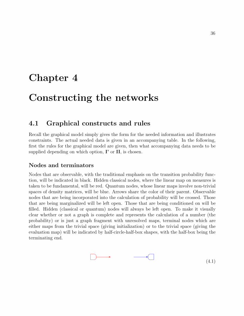
36
Chapter 4
Constructing the networks
4.1 Graphical constructs and rules
Recall the graphical model simply gives the form for the needed information and illustratesconstraints. The actual needed data is given in an accompanying table. In the following,first the rules for the graphical model are given, then what accompanying data needs to besupplied depending on which option, I’ or II, is chosen.
Nodes and terminators
Nodes that are observable, with the traditional emphasis on the transition probability func-tion, will be indicated in black. Hidden classical nodes, where the linear map on measures istaken to be fundamental, will be red. Quantum nodes, whose linear maps involve non-trivialspaces of density matrices, will be blue. Arrows share the color of their parent. Observablenodes that are being incorporated into the calculation of probability will be crossed. Thosethat are being marginalized will be left open. Those that are being conditioned on will befilled. Hidden (classical or quantum) nodes will always be left open. To make it visuallyclear whether or not a graph is complete and represents the calculation of a number (theprobability) or is just a graph fragment with unresolved maps, terminal nodes which areeither maps from the trivial space (giving initialization) or to the trivial space (giving theevaluation map) will be indicated by half-circle-half-box shapes, with the half-box being theterminating end.
--
(4.1)

CHAPTER 4. CONSTRUCTING THE NETWORKS 37
Splitters
As has been pointed out (see §2.4), the usual Bayesian network construction depends heavilyon the ability to copy, with each child node receiving a copy. Without this ability (see §3.2and §3.4), an additional graphical structure is required, the splitter. This is an oval withone or more arrows coming in and more than one arrow coming out–if only one arrow comesout, the splitter can be dispensed with and all the incoming arrows can be redirected to thefollowing node.
-
HHHHj
-*
(4.2)
Pince-nez
There is a certain construction that occurs so often for joining hidden nodes to observableones that it is replaced by its own structure, the pince-nez. As the name suggests, this istwo circles, one an observable node, the other a hidden one, joined by a bar.
m1Ô⇒ m1HHHj
1@@R m mPPPPq-- HHHj
-(4.3)
The neutral term pince-nez is employed since the concept of “measurement”1 applied tohidden nodes is so fraught with metaphysical connotations.
4.2 Data for the structures using Option I’
Using option I’, for each hidden node, the most general data is
(I, µ,H;O, ν, J;L)
where I is the input set, µ the accompanying base measure, H the input Hilbert space,O the output set, ν the accompanying base measure, J the output Hilbert space, and L acompletely-positive, norm-preserving (on the positive cone) map in B(L1(I;µ;D(H)), L1(O;ν;D(J))). If either Hilbert spaces are the trivial space C, it can be left off the list. Similarly,if either base measure is trivial, for instance, if µ(∅) = 0, µ(I) = 1 with no other setsmeasurable, then it and its set can be left out as well.
1We will always place “measurement” in quotation marks to emphasize its problematic nature.
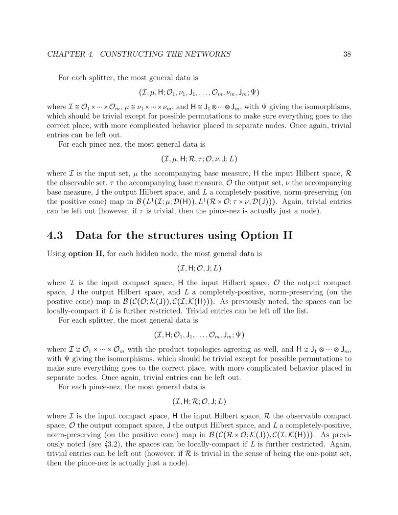
CHAPTER 4. CONSTRUCTING THE NETWORKS 38
For each splitter, the most general data is
(I, µ,H;O1, ν1, J1, . . . ,Om, νm, Jm; Ψ)
where I ≅ O1×⋯×Om, µ ≅ ν1×⋯×νm, and H ≅ J1⊗⋯⊗Jm, with Ψ giving the isomorphisms,which should be trivial except for possible permutations to make sure everything goes to thecorrect place, with more complicated behavior placed in separate nodes. Once again, trivialentries can be left out.
For each pince-nez, the most general data is
(I, µ,H;R, τ ;O, ν, J;L)
where I is the input set, µ the accompanying base measure, H the input Hilbert space, Rthe observable set, τ the accompanying base measure, O the output set, ν the accompanyingbase measure, J the output Hilbert space, and L a completely-positive, norm-preserving (onthe positive cone) map in B (L1(I;µ;D(H)), L1(R ×O; τ × ν;D(J))). Again, trivial entriescan be left out (however, if τ is trivial, then the pince-nez is actually just a node).
4.3 Data for the structures using Option II
Using option II, for each hidden node, the most general data is
(I,H;O, J;L)
where I is the input compact space, H the input Hilbert space, O the output compactspace, J the output Hilbert space, and L a completely-positive, norm-preserving (on thepositive cone) map in B (C(O;K(J)),C(I;K(H))). As previously noted, the spaces can belocally-compact if L is further restricted. Trivial entries can be left off the list.
For each splitter, the most general data is
(I,H;O1, J1, . . . ,Om, Jm; Ψ)
where I ≅ O1 × ⋯ ×Om with the product topologies agreeing as well, and H ≅ J1 ⊗⋯ ⊗ Jm,with Ψ giving the isomorphisms, which should be trivial except for possible permutations tomake sure everything goes to the correct place, with more complicated behavior placed inseparate nodes. Once again, trivial entries can be left out.
For each pince-nez, the most general data is
(I,H;R;O, J;L)
where I is the input compact space, H the input Hilbert space, R the observable compactspace, O the output compact space, J the output Hilbert space, and L a completely-positive,norm-preserving (on the positive cone) map in B (C(R ×O;K(J)),C(I;K(H))). As previ-ously noted (see §3.2), the spaces can be locally-compact if L is further restricted. Again,trivial entries can be left out (however, if R is trivial in the sense of being the one-point set,then the pince-nez is actually just a node).

CHAPTER 4. CONSTRUCTING THE NETWORKS 39
4.4 Example-double-slit experiment
So far, the exposition has been quite abstract. To make things more concrete and demon-strate how to use Bayesian networks with linear maps (both classical and quantum) inpractice, consider the following example. There is a black-box with a dial which can be setto any position θ on a circle, a switch with two settings, and four lights, with lights one andtwo forming one pair and lights three and four forming another. After study, it is determinedto have the following properties: if the switch is off, periodically one of the second pair oflights flashes while the first pair never flashes, whereas, if the switch is on, one of each pairflashes. After more study, it is determined the behavior of each round is independent and,if the switch is off, with probability cos2 θ the third light alone flashes and with probabilitysin2 θ the fourth light alone flashes. If the switch is on, the joint probabilities are as follows:
first on, third on, others off 14
first on, fourth on, others off 14
second on, third on, others off 14
second on, fourth on, others off 14
(4.4)
with the other probabilities being zero. Presenting the information in the manner of thepreceding joint probabilities corresponds to the following graphical model:
m m dial switch
first pair of lights second pair of lights
HHHHH
HH
(4.5)
Suppose the box is now opened and is found to be composed of five modules. A cableruns from the first module to the second. Two cables come from the second module, oneeach running to a pair of seemingly identical modules, each of which has one of the first pairof lights. The switch activates switches on the pair in unison. These modules have cablesrunning to the last, which has the dial as a control. If possible, given the joint probabilities,we should confine ourselves to models which are consistent with the constraints implied bythese observations because we would like to be able to predict what would happen if thesemodules were rewired or taken out and placed in a different context.
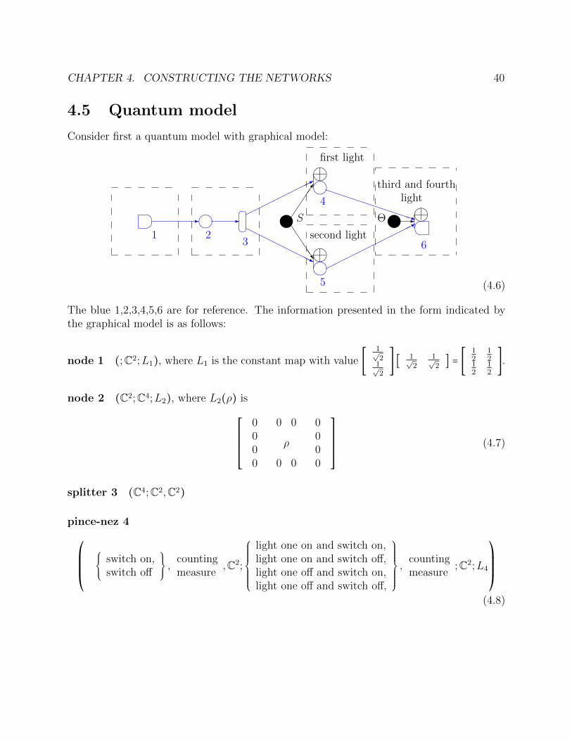
CHAPTER 4. CONSTRUCTING THE NETWORKS 40
4.5 Quantum model
Consider first a quantum model with graphical model:
-
1
m2
-
3
*
HHHHH
HHHj m5
m4
*
PPPPPPPPPPq6m
mm
second light
first light
third and fourthlight
ΘSJJJJ
-
(4.6)
The blue 1,2,3,4,5,6 are for reference. The information presented in the form indicated bythe graphical model is as follows:
node 1 (;C2;L1), where L1 is the constant map with value [1√2
1√2
] [ 1√2
1√2
] = [12
12
12
12
].
node 2 (C2;C4;L2), where L2(ρ) is
⎡⎢⎢⎢⎢⎢⎢⎢⎣
0 0 0 000
ρ00
0 0 0 0
⎤⎥⎥⎥⎥⎥⎥⎥⎦
(4.7)
splitter 3 (C4;C2,C2)
pince-nez 4
⎛⎜⎜⎜⎝
switch on,switch off
, countingmeasure
,C2;
⎧⎪⎪⎪⎪⎪⎨⎪⎪⎪⎪⎪⎩
light one on and switch on,light one on and switch off,light one off and switch on,light one off and switch off,
⎫⎪⎪⎪⎪⎪⎬⎪⎪⎪⎪⎪⎭
,countingmeasure
;C2;L4
⎞⎟⎟⎟⎠
(4.8)

CHAPTER 4. CONSTRUCTING THE NETWORKS 41
where L4(τ) is
⎧⎪⎪⎪⎪⎪⎪⎪⎪⎪⎪⎪⎪⎪⎪⎨⎪⎪⎪⎪⎪⎪⎪⎪⎪⎪⎪⎪⎪⎪⎩
τ ∣switch off if light one off and switch off
0 if light one on and switch off⎡⎢⎢⎢⎢⎣
1 0
0 0
⎤⎥⎥⎥⎥⎦τ ∣switch on
⎡⎢⎢⎢⎢⎣
1 0
0 0
⎤⎥⎥⎥⎥⎦if first on and switch on
⎡⎢⎢⎢⎢⎣
0 0
0 1
⎤⎥⎥⎥⎥⎦τ ∣switch on
⎡⎢⎢⎢⎢⎣
0 0
0 1
⎤⎥⎥⎥⎥⎦if first off and switch on
(4.9)
pince-nez 5 Same as for pince-nez 4 except the second light replaces the first light.
pince-nez 6
⎛⎜⎜⎜⎝[0,2π), Lebesgue
measure,C4;
⎧⎪⎪⎪⎪⎪⎨⎪⎪⎪⎪⎪⎩
third and fourth on,third on,fourth on,third and fourth off
⎫⎪⎪⎪⎪⎪⎬⎪⎪⎪⎪⎪⎭
,countingmeasure
; ;L6
⎞⎟⎟⎟⎠
where L6(τ) is
∫2π
0[ 1 0 0 0 ] τ(θ)
⎡⎢⎢⎢⎢⎢⎢⎢⎣
1000
⎤⎥⎥⎥⎥⎥⎥⎥⎦
dθ if both third and fourth on (4.10)
∫2π
0[ 0 1√
2eıθ 1√
2e−ıθ 0 ] τ(θ)
⎡⎢⎢⎢⎢⎢⎢⎢⎢⎣
01√2e−ıθ
1√2eıθ
0
⎤⎥⎥⎥⎥⎥⎥⎥⎥⎦
dθ if third on
∫2π
0[ 0 1√
2eıθ − 1√
2e−ıθ 0 ] τ(θ)
⎡⎢⎢⎢⎢⎢⎢⎢⎢⎣
01√2e−ıθ
− 1√2eıθ
0
⎤⎥⎥⎥⎥⎥⎥⎥⎥⎦
dθ if fourth on
∫2π
0[ 0 0 0 1 ] τ(θ)
⎡⎢⎢⎢⎢⎢⎢⎢⎣
0001
⎤⎥⎥⎥⎥⎥⎥⎥⎦
dθ if both third and fourth off
Using this information, the joint probability, given that the switch is off and the dial is set
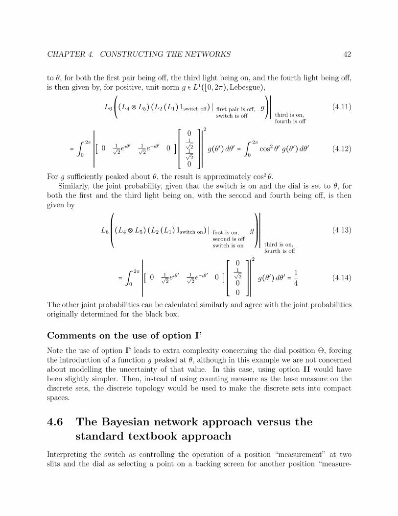
CHAPTER 4. CONSTRUCTING THE NETWORKS 42
to θ, for both the first pair being off, the third light being on, and the fourth light being off,is then given by, for positive, unit-norm g ∈ L1([0,2π),Lebesgue),
L6
⎛⎝(L4 ⊗L5) (L2 (L1)1switch off) ∣ first pair is off,
switch is off
g⎞⎠
RRRRRRRRRRRR third is on,fourth is off
(4.11)
= ∫2π
0
RRRRRRRRRRRRRRRRRRR
[ 0 1√2eıθ
′ 1√2e−ıθ
′0 ]
⎡⎢⎢⎢⎢⎢⎢⎢⎢⎣
01√2
1√2
0
⎤⎥⎥⎥⎥⎥⎥⎥⎥⎦
RRRRRRRRRRRRRRRRRRR
2
g(θ′)dθ′ = ∫2π
0cos2 θ′ g(θ′)dθ′ (4.12)
For g sufficiently peaked about θ, the result is approximately cos2 θ.Similarly, the joint probability, given that the switch is on and the dial is set to θ, for
both the first and the third light being on, with the second and fourth being off, is thengiven by
L6
⎛⎜⎜⎜⎝(L4 ⊗L5) (L2 (L1)1switch on) ∣ first is on,
second is offswitch is on
g
⎞⎟⎟⎟⎠
RRRRRRRRRRRRRRRRRR third is on,fourth is off
(4.13)
= ∫2π
0
RRRRRRRRRRRRRRRRRRR
[ 0 1√2eıθ
′ 1√2e−ıθ
′0 ]
⎡⎢⎢⎢⎢⎢⎢⎢⎣
01√2
00
⎤⎥⎥⎥⎥⎥⎥⎥⎦
RRRRRRRRRRRRRRRRRRR
2
g(θ′)dθ′ = 1
4(4.14)
The other joint probabilities can be calculated similarly and agree with the joint probabilitiesoriginally determined for the black box.
Comments on the use of option I’
Note the use of option I’ leads to extra complexity concerning the dial position Θ, forcingthe introduction of a function g peaked at θ, although in this example we are not concernedabout modelling the uncertainty of that value. In this case, using option II would havebeen slightly simpler. Then, instead of using counting measure as the base measure on thediscrete sets, the discrete topology would be used to make the discrete sets into compactspaces.
4.6 The Bayesian network approach versus the
standard textbook approach
Interpreting the switch as controlling the operation of a position “measurement” at twoslits and the dial as selecting a point on a backing screen for another position “measure-
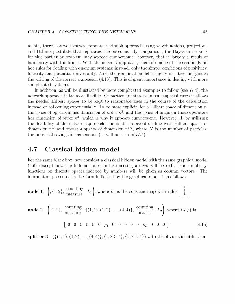
CHAPTER 4. CONSTRUCTING THE NETWORKS 43
ment”, there is a well-known standard textbook approach using wavefunctions, projectors,and Bohm’s postulate that replicates the outcome. By comparison, the Bayesian networkfor this particular problem may appear cumbersome; however, that is largely a result offamiliarity with the firmer. With the network approach, there are none of the seemingly adhoc rules for dealing with quantum systems; instead, only the simple conditions of positivity,linearity and potential universality. Also, the graphical model is highly intuitive and guidesthe writing of the correct expression (4.13). This is of great importance in dealing with morecomplicated systems.
In addition, as will be illustrated by more complicated examples to follow (see §7.4), thenetwork approach is far more flexible. Of particular interest, in some special cases it allowsthe needed Hilbert spaces to be kept to reasonable sizes in the course of the calculationinstead of ballooning exponentially. To be more explicit, for a Hilbert space of dimension n,the space of operators has dimension of order n2, and the space of maps on these operatorshas dimension of order n4, which is why it appears cumbersome. However, if, by utilizingthe flexibility of the network approach, one is able to avoid dealing with Hilbert spaces ofdimension nN and operator spaces of dimension n2N , where N is the number of particles,the potential savings is tremendous (as will be seen in §7.4).
4.7 Classical hidden model
For the same black box, now consider a classical hidden model with the same graphical model(4.6) (except now the hidden nodes and connecting arrows will be red). For simplicity,functions on discrete spaces indexed by numbers will be given as column vectors. Theinformation presented in the form indicated by the graphical model is as follows:
node 1 (;1,2, countingmeasure
;L1), where L1 is the constant map with value [1212
].
node 2 (1,2, countingmeasure
;(1,1), (1,2), . . . , (4,4), countingmeasure
;L2), where L2(ρ) is
[ 0 0 0 0 0 0 ρ1 0 0 0 0 0 ρ2 0 0 0 ]T(4.15)
splitter 3 ((1,1), (1,2), . . . , (4,4);1,2,3,4,1,2,3,4) with the obvious identification.
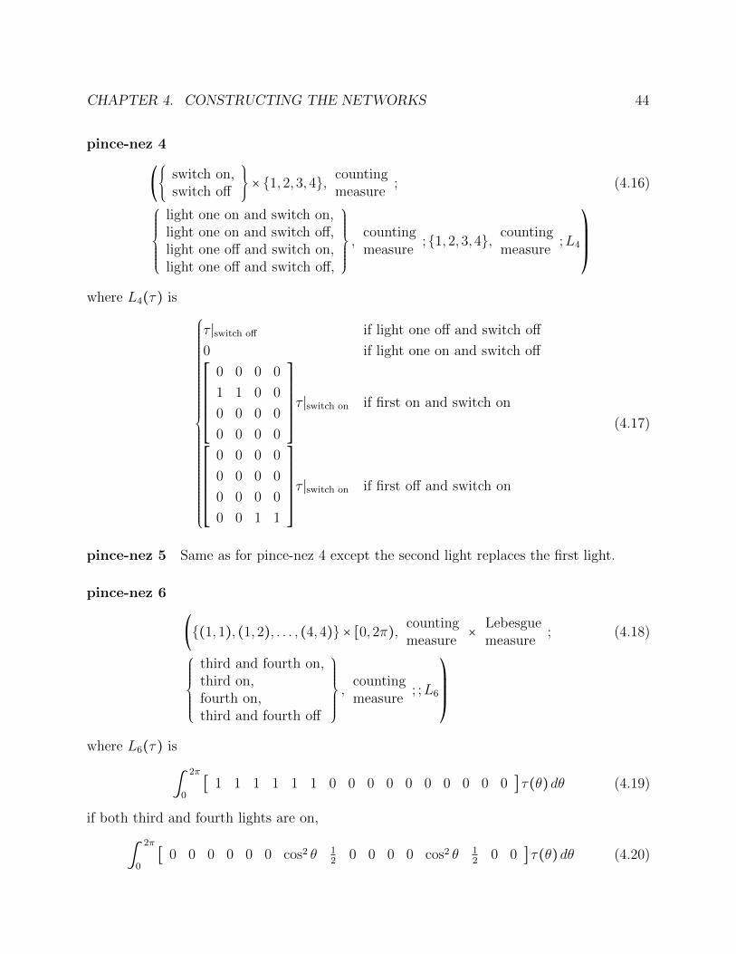
CHAPTER 4. CONSTRUCTING THE NETWORKS 44
pince-nez 4
( switch on,switch off
× 1,2,3,4, countingmeasure
; (4.16)
⎧⎪⎪⎪⎪⎪⎨⎪⎪⎪⎪⎪⎩
light one on and switch on,light one on and switch off,light one off and switch on,light one off and switch off,
⎫⎪⎪⎪⎪⎪⎬⎪⎪⎪⎪⎪⎭
,countingmeasure
;1,2,3,4, countingmeasure
;L4
⎞⎟⎟⎟⎠
where L4(τ) is
⎧⎪⎪⎪⎪⎪⎪⎪⎪⎪⎪⎪⎪⎪⎪⎪⎪⎪⎪⎪⎪⎪⎪⎪⎪⎪⎨⎪⎪⎪⎪⎪⎪⎪⎪⎪⎪⎪⎪⎪⎪⎪⎪⎪⎪⎪⎪⎪⎪⎪⎪⎪⎩
τ ∣switch off if light one off and switch off
0 if light one on and switch off⎡⎢⎢⎢⎢⎢⎢⎢⎢⎢⎣
0 0 0 0
1 1 0 0
0 0 0 0
0 0 0 0
⎤⎥⎥⎥⎥⎥⎥⎥⎥⎥⎦
τ ∣switch on if first on and switch on
⎡⎢⎢⎢⎢⎢⎢⎢⎢⎢⎣
0 0 0 0
0 0 0 0
0 0 0 0
0 0 1 1
⎤⎥⎥⎥⎥⎥⎥⎥⎥⎥⎦
τ ∣switch on if first off and switch on
(4.17)
pince-nez 5 Same as for pince-nez 4 except the second light replaces the first light.
pince-nez 6
((1,1), (1,2), . . . , (4,4) × [0,2π), countingmeasure
× Lebesguemeasure
; (4.18)
⎧⎪⎪⎪⎪⎪⎨⎪⎪⎪⎪⎪⎩
third and fourth on,third on,fourth on,third and fourth off
⎫⎪⎪⎪⎪⎪⎬⎪⎪⎪⎪⎪⎭
,countingmeasure
; ;L6
⎞⎟⎟⎟⎠
where L6(τ) is
∫2π
0[ 1 1 1 1 1 1 0 0 0 0 0 0 0 0 0 0 ] τ(θ)dθ (4.19)
if both third and fourth lights are on,
∫2π
0[ 0 0 0 0 0 0 cos2 θ 1
2 0 0 0 0 cos2 θ 12 0 0 ] τ(θ)dθ (4.20)
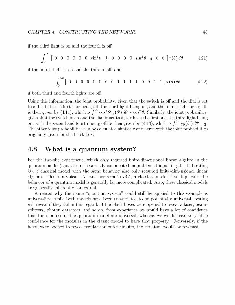
CHAPTER 4. CONSTRUCTING THE NETWORKS 45
if the third light is on and the fourth is off,
∫2π
0[ 0 0 0 0 0 0 sin2 θ 1
2 0 0 0 0 sin2 θ 12 0 0 ] τ(θ)dθ (4.21)
if the fourth light is on and the third is off, and
∫2π
0[ 0 0 0 0 0 0 0 0 1 1 1 1 0 0 1 1 ] τ(θ)dθ (4.22)
if both third and fourth lights are off.
Using this information, the joint probability, given that the switch is off and the dial is setto θ, for both the first pair being off, the third light being on, and the fourth light being off,is then given by (4.11), which is ∫
2π
0 cos2 θ′ g(θ′)dθ′ ≈ cos2 θ. Similarly, the joint probability,given that the switch is on and the dial is set to θ, for both the first and the third light beingon, with the second and fourth being off, is then given by (4.13), which is ∫
2π
014g(θ′)dθ′ = 1
4 .The other joint probabilities can be calculated similarly and agree with the joint probabilitiesoriginally given for the black box.
4.8 What is a quantum system?
For the two-slit experiment, which only required finite-dimensional linear algebra in thequantum model (apart from the already commented on problem of inputting the dial settingΘ), a classical model with the same behavior also only required finite-dimensional linearalgebra. This is atypical. As we have seen in §3.5, a classical model that duplicates thebehavior of a quantum model is generally far more complicated. Also, these classical modelsare generally inherently contextual.
A reason why the name “quantum system” could still be applied to this example isuniversality: while both models have been constructed to be potentially universal, testingwill reveal if they fail in this regard. If the black boxes were opened to reveal a laser, beam-splitters, photon detectors, and so on, from experience we would have a lot of confidencethat the modules in the quantum model are universal, whereas we would have very littleconfidence for the modules in the classic model to have that property. Conversely, if theboxes were opened to reveal regular computer circuits, the situation would be reversed.

46
Chapter 5
Relation to textbook quantummechanics
5.1 Textbook rules for quantum mechanics
The quantum Bayesian network structure developed so far has constraints only arising fromthe requirements of positivity, linearity, and potential universality. It is not obvious that ithas any connection necessarily to what is usually thought of as quantum mechanics. Usingoption I’, that is not the situation, as is shown below.
However, while the following justifies the usage of the name quantum for the extendedBayesian networks, it should not be taken as a justification of them–quite the opposite. TheBayesian network approach is predicated on a very reasonable basis. The textbook approachto quantum mechanics is only comfortable due to familiarity; on its own merits its rules areincomprehensible and unmotivated. Hence, the following is better taken as a justificationof the textbook approach. In other words, if quantum behavior had first been discoveredas forecasting arising from a reasonable extension of Bayesian networks, and the usual listof textbook rules were later discovered picking out a certain subset of networks that weresufficient to model any situation, no one would take those rules as primary.
Rule one
Textbook quantum mechanics imposes an additional rule: only networks in the form ofchains are permitted and all the Hilbert spaces along a chain must be the same (apart forterminating trivial spaces). (This rule may arise from imagining that we have some sortof universal, initial-value, dynamical system). Mathematically, this rule puts no additionalconstraints on the network formulation; it is always possible to obey this by working in asufficiently large Hilbert space and waiting until the end of the calculation to perform thereduced traces arising from terminal nodes. However, doing this in practice is unnecessarilydifficult–the whole point of Bayesian networks is to try to find a model made of simple and
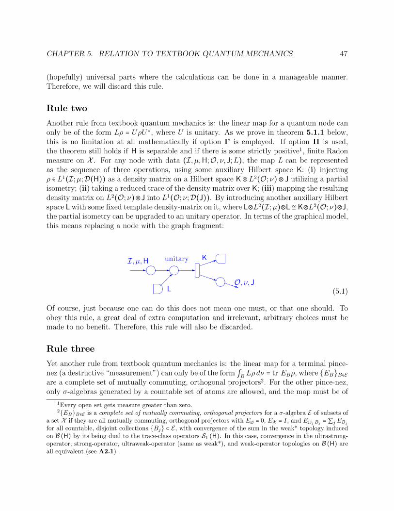
CHAPTER 5. RELATION TO TEXTBOOK QUANTUM MECHANICS 47
(hopefully) universal parts where the calculations can be done in a manageable manner.Therefore, we will discard this rule.
Rule two
Another rule from textbook quantum mechanics is: the linear map for a quantum node canonly be of the form Lρ = UρU∗, where U is unitary. As we prove in theorem 5.1.1 below,this is no limitation at all mathematically if option I’ is employed. If option II is used,the theorem still holds if H is separable and if there is some strictly positive1, finite Radonmeasure on X . For any node with data (I, µ,H;O, ν, J;L), the map L can be representedas the sequence of three operations, using some auxiliary Hilbert space K: (i) injectingρ ∈ L1(I;µ;D(H)) as a density matrix on a Hilbert space K⊗L2(O;ν)⊗ J utilizing a partialisometry; (ii) taking a reduced trace of the density matrix over K; (iii) mapping the resultingdensity matrix on L2(O;ν)⊗J into L1(O;ν;D(J)). By introducing another auxiliary Hilbertspace L with some fixed template density-matrix on it, where L⊗L2(I;µ)⊗L ≅ K⊗L2(O;ν)⊗J,the partial isometry can be upgraded to an unitary operator. In terms of the graphical model,this means replacing a node with the graph fragment:
m
m m
unitary-1
PPPqPPPq
I, µ,H
L
K
O, ν, J
-
-
(5.1)
Of course, just because one can do this does not mean one must, or that one should. Toobey this rule, a great deal of extra computation and irrelevant, arbitrary choices must bemade to no benefit. Therefore, this rule will also be discarded.
Rule three
Yet another rule from textbook quantum mechanics is: the linear map for a terminal pince-nez (a destructive “measurement”) can only be of the form ∫B Lρdν = tr EBρ, where EBB∈Eare a complete set of mutually commuting, orthogonal projectors2. For the other pince-nez,only σ-algebras generated by a countable set of atoms are allowed, and the map must be of
1Every open set gets measure greater than zero.2EBB∈E is a complete set of mutually commuting, orthogonal projectors for a σ-algebra E of subsets of
a set X if they are all mutually commuting, orthogonal projectors with E∅ = 0, EX = I, and E⋃j Bj = ∑j EBj
for all countable, disjoint collections Bj ⊂ E , with convergence of the sum in the weak* topology inducedon B (H) by its being dual to the trace-class operators S1 (H). In this case, convergence in the ultrastrong-operator, strong-operator, ultraweak-operator (same as weak*), and weak-operator topologies on B (H) areall equivalent (see A2.1).
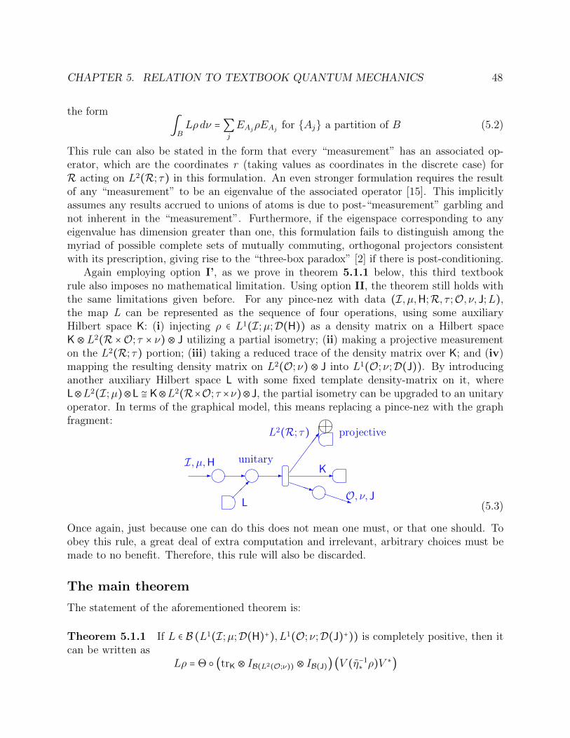
CHAPTER 5. RELATION TO TEXTBOOK QUANTUM MECHANICS 48
the form
∫BLρdν =∑
j
EAjρEAj for Aj a partition of B (5.2)
This rule can also be stated in the form that every “measurement” has an associated op-erator, which are the coordinates r (taking values as coordinates in the discrete case) forR acting on L2(R; τ) in this formulation. An even stronger formulation requires the resultof any “measurement” to be an eigenvalue of the associated operator [15]. This implicitlyassumes any results accrued to unions of atoms is due to post-“measurement” garbling andnot inherent in the “measurement”. Furthermore, if the eigenspace corresponding to anyeigenvalue has dimension greater than one, this formulation fails to distinguish among themyriad of possible complete sets of mutually commuting, orthogonal projectors consistentwith its prescription, giving rise to the “three-box paradox” [2] if there is post-conditioning.
Again employing option I’, as we prove in theorem 5.1.1 below, this third textbookrule also imposes no mathematical limitation. Using option II, the theorem still holds withthe same limitations given before. For any pince-nez with data (I, µ,H;R, τ ;O, ν, J;L),the map L can be represented as the sequence of four operations, using some auxiliaryHilbert space K: (i) injecting ρ ∈ L1(I;µ;D(H)) as a density matrix on a Hilbert spaceK ⊗ L2(R ×O; τ × ν) ⊗ J utilizing a partial isometry; (ii) making a projective measurementon the L2(R; τ) portion; (iii) taking a reduced trace of the density matrix over K; and (iv)mapping the resulting density matrix on L2(O;ν) ⊗ J into L1(O;ν;D(J)). By introducinganother auxiliary Hilbert space L with some fixed template density-matrix on it, whereL⊗L2(I;µ)⊗L ≅ K⊗L2(R×O; τ ×ν)⊗J, the partial isometry can be upgraded to an unitaryoperator. In terms of the graphical model, this means replacing a pince-nez with the graphfragment: m
m
m m
unitary
projective
- -PPPq
7
PPPq
I, µ,H
L
K
O, ν, J
L2(R; τ)
-
-
(5.3)
Once again, just because one can do this does not mean one must, or that one should. Toobey this rule, a great deal of extra computation and irrelevant, arbitrary choices must bemade to no benefit. Therefore, this rule will also be discarded.
The main theorem
The statement of the aforementioned theorem is:
Theorem 5.1.1 If L ∈ B (L1(I;µ;D(H)+), L1(O;ν;D(J)+)) is completely positive, then itcan be written as
Lρ = Θ (trK ⊗ IB(L2(O;ν)) ⊗ IB(J)) (V (η−1∗ ρ)V ∗)
CHAPTER 5. RELATION TO TEXTBOOK QUANTUM MECHANICS 49
for some Hilbert space K, some map η−1∗ ∶ L1(I;µ;D(H)+)→ D (L2(I;µ)⊗H)+, some partial
isometry V ∶ L2(I;µ) ⊗ H → K ⊗ L2(O;ν) ⊗ J, and some map Θ ∶ D (L2(O;ν)⊗ J)+ →L1(O;ν;D(J)+). If all the Hilbert spaces are finite dimensional, the dimension of K is lessthan or equal to the product of dimensions dim J dimH dimL2(I;µ).
Comments Writing L in the preceding form gives the behavior asserted above for thepince-nez since, rewriting O →R×O and ν → τ ×ν, then for any τ -measurable subset B ⊂R,the map Θ is such that
∫BLρdτ = Θ′ (trK ⊗ P (B)⊗ IB(L2(O;ν)) ⊗ IB(J)) (V (η−1
∗ ρ)V ∗) (5.4)
where P (B) is the functional on D(L2(O;ν)) given by P (B)τ = ∫x∈B τ(x,x)dν(x) and Θ′ is some map from D (L2(O;ν)⊗ J)+ to L1(O;ν;D(J)+). The assertion for thenode follows since a node is a pince-nez with trivial base measure τ for R.
From C5.12, the theorem also holds for option II as long as the given conditions areheld: H is separable (so there is some strictly positive density matrix on it) and there is somestrictly positive, finite Radon measure µ on X (without strict positivity, some of the neededinverses will not exist). Note that from C5.12, it is not possible to choose ν arbitrarily; itdepends on both µ and the map L. Then we have
L(1B ⊗ f) = η−1 (V ∗ (IK ⊗ π(1B)⊗ η(f))V ) (5.5)
where π(g) is the operator on L2(R; τ) given by pointwise multiplication by g for anyg ∈ L∞(R; τ)), η−1 ∶ B (L2(I;µ)⊗H)+ → L∞(X ;µ;K(H))–which contains C(X ;K(H))–andη ∶ C(Y;K(J))+ → B(L2(O;ν)⊗ J)+.
The following proof, together with a following lemma and several supporting proposi-tions in the appendix, is quite lengthy. The main idea is to recognize that the dual space todensity-matrix-valued, L1-functions is a von Neumann algebra3. Then one result by Stine-spring [88] on completely-positive maps on C∗-algebras and another result by Sakai [79]on representations of von Neumann algebras provide the core. Most of the rest is just thetedious work of proving the preconditions necessary for these two results apply.
Proof Start with any such L. Extend L to L1(I;µ;S1(H)) using B5.15 and B5.164. Linduces an adjoint map L∗ ∶ L1(O;ν;S1(J))∗ → L1(I;µ;S1(H))∗ by L∗(Φ)ρ = Φ(Lρ). ByB5.19, there is a weakly-continuous, isometric bijection η ∶ L1(O;ν;S1(J))∗ → W(O;ν; J),where W(O;ν; J) ⊂ B(L2(O;ν) ⊗ H) is a von Neumann algebra with unit. The bijec-tion therefore induces a C *-algebra structure on L1(O;ν;S1(J))∗ with W *- representa-tion5 (η,L2(O;ν) ⊗ J). Also by B5.19, there is a weakly-continuous, isometric bijection
3A Banach algebra is a Banach space equipped with an associative, distributive product satisfying ∥ab∥ ≤∥a∥∥b∥. A *-algebra is a Banach algebra with an antilinear involution. A C*-algebra is a *-algebra where∥a∗a∥ = ∥a∥2. A von Neumann algebra (also termed a W*-algebra) is a C *-algebra which, as a Banach space,is a dual space.
4S1(H) denotes all trace-class operators on H.5A W*-representation has a weakly-continuous map.
CHAPTER 5. RELATION TO TEXTBOOK QUANTUM MECHANICS 50
η ∶ L1(I;µ;S1(H))∗ →W(I;µ;H) ⊂ B(L2(I;µ)⊗H). By B5.20, η L∗ is completely-positive(in the sense required for Stinespring’s theorem). Therefore, by Stinespring’s theorem[88],η L∗(Φ) = V ∗ζ(Φ)V for some Hilbert space M, some representation (ζ,M), and someV ∈ B(L2(I;µ)⊗H,M).
By lemma 5.1.2 below, (ζ,M) is a W *-representation. Therefore, since η is faithful,(ζ,M) is related to (η,L2(O;ν)⊗J) (up to unitary equivalence) by an amplification composedwith an induction[79]: ζ(Φ) = W ∗E (IK ⊗ η(Φ))W for some Hilbert space K with M =K ⊗ L2(O;ν) ⊗ J, some orthogonal projector E in the commutant of IK ⊗W(O;ν; J), andsome unitary operator W ∈ B(M). However, W and E can be absorbed into a redefinitionof V , V → EWV , so ζ can be taken to be simply the amplification of η, ζΦ = IK ⊗ (ηΦ).
Then, for any Φ ∈ L1(I;µ;D(H))∗ and ρ ∈ L1(I;µ;D(H)+),ΦLρ = (L∗Φ)ρ = ((η−1 η L∗)Φ)ρ = (V ∗ (IK ⊗ ηΦ)V ) η−1
∗ ρ (5.6)
= (IK ⊗ ηΦ)V (η−1∗ ρ)V ∗
= (ηΦ) ((trK ⊗ IB(L2(O;ν)) ⊗ IB(J))V (η−1∗ ρ)V ∗)
= Φ (Θ (trK ⊗ IB(L2(O;ν)) ⊗ IB(J))V (η−1∗ ρ)V ∗)
where Θ and η−1∗ are defined in B5.19 (note η−1
∗ is only defined up to equivalence class, butthe choice of element within this class is of no consequence). Since Φ was arbitrary, thedesired form has been demonstrated.
Since L is an isometry on the positive cone, for any ρ in this cone with ∥ρ∥ = 1,
1 = ∥Lρ∥ = Φ (Θ (trK ⊗ IB(L2(O;ν)) ⊗ IB(J))V (η−1∗ ρ)V ∗) (5.7)
= η−1 (V ∗ (IK ⊗ ηΦ)V )ρwhere Φ is the functional ϕ→ ∫O trJϕ dν. However, then ηΦ = IL2(O;ν) ⊗ IJ, so we have
1 = η−1 (V ∗V )ρ (5.8)
In order for η−1 (V ∗V ) to be the functional ρ→ ∫I trHρ dµ, it must be that V ∗V = IL2(I;µ)⊗IH,so V is a partial isometry.
Furthermore, if all the Hilbert spaces are finite-dimensional, it is possible to boundthe dimension of K. By B5.21, the Hilbert space L2(O;ν) ⊗ S2(J) ≅ L2(O;ν;S2(J)) isrelatively dense within W(O;ν; J) in the ultrastrong-operator topology. Therefore, givenany ∑m
j=1 Φj ⊗ φj ∈ L1 (O;ν;S1(J))∗ ⊗ (L2(I;µ) ⊗ H) and ε > 0, there is a subset Ψj ⊂η−1 (W ∩L2(O;ν)⊗ S2(J)) such that6
ε >m
∑j,k=1
((Φk −Ψk)⋆ (Φj −Ψj))L (η∗(φjφ∗k)) (5.9)
=m
∑j,k=1
⟨(η L∗) ((Φk −Ψk)⋆ (Φj −Ψj))φj, φk⟩
6To avoid confusion with the adjoint map Φ∗ ∶ C→ L1 (X ;µ;S1(H))∗, ⋆ is used to indicate the conjugate
within the von Neumann algebra, with Φ⋆ = η−1 (η(Φ)∗). However, if the dual pairs ⟨w, z⟩ for w, z ∈ Z and⟨L,Φ⟩ are taken complex, with values wz and Φ⋆L respectively, then Φ∗z = zΦ⋆.
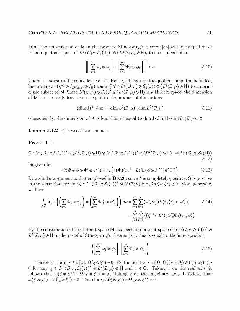
CHAPTER 5. RELATION TO TEXTBOOK QUANTUM MECHANICS 51
From the construction of M in the proof to Stinespring’s theorem[88] as the completion ofcertain quotient space of L1 (O;ν;S1(J))∗ ⊗ (L2(I;µ)⊗H), this is equivalent to
∥[m
∑j=1
Φj ⊗ φj] − [m
∑k=1
Ψk ⊗ φk]∥2
< ε (5.10)
where [⋅] indicates the equivalence class. Hence, letting ι be the quotient map, the bounded,linear map ι (η−1 ⊗ IL2(I;µ) ⊗ IH) sends (W ∩L2(O;ν)⊗ S2(J))⊗ (L2(I;µ)⊗H) to a norm-dense subset of M. Since L2(O;ν)⊗S2(J)⊗ (L2(I;µ)⊗H) is a Hilbert space, the dimensionof M is necessarily less than or equal to the product of dimensions:
(dim J)2 ⋅ dimH ⋅ dimL2(I;µ) ⋅ dimL2(O;ν) (5.11)
consequently, the dimension of K is less than or equal to dim J ⋅ dimH ⋅ dimL2(I;µ). ◻
Lemma 5.1.2 ζ is weak*-continuous.
Proof Let
Ω ∶ L1 (O;ν;S1(J))∗⊗ (L2(I;µ)⊗H)⊗L1 (O;ν;S1(J))∗⊗ (L2(I;µ)⊗H)∗ → L1 (O;µ;S1(H))(5.12)
be given byΩ(Φ⊗ φ⊗Φ′ ⊗ φ′∗) = η∗ (η(Φ)(η−1
∗ L(η∗(φ⊗ φ′∗))η(Φ′)) (5.13)
By a similar argument to that employed in B5.20, since L is completely-positive, Ω is positivein the sense that for any ξ ∈ L1 (O;ν;S1(J))∗ ⊗L2(I;µ)⊗H, Ω(ξ ⊗ ξ∗) ≥ 0. More generally,we have
∫O
trJΩ((m
∑j=1
Φj ⊗ ψj)⊗ (n
∑k=1
Φ′⋆
k ⊗ ψ′∗
k)) dν =m
∑j=1
n
∑k=1
(Φ′⋆
kΦj)L(η∗(φj ⊗ φ′∗k) (5.14)
=m
∑j=1
n
∑k=1
⟨(η−1 L∗)(Φ′⋆
kΦj)ψj, ψ′k⟩
By the construction of the Hilbert space M as a certain quotient space of L1 (O;ν;S1(J))∗⊗L2(I;µ)⊗H in the proof of Stinespring’s theorem[88], this is equal to the inner-product
⟨[m
∑j=1
Φj ⊗ ψj] , [n
∑k=1
Φ′k ⊗ ψ′k]⟩ (5.15)
Therefore, for any ξ ∈ [0], Ω(ξ⊗ ξ∗) = 0. By the positivity of Ω, Ω((χ+ zξ)⊗ (χ+ zξ)∗) ≥0 for any χ ∈ L1 (O;ν;S1(J))∗ ⊗ L2(I;µ) ⊗ H and z ∈ C. Taking z on the real axis, itfollows that Ω(ξ ⊗ χ∗) + Ω(χ ⊗ ξ∗) = 0. Taking z on the imaginary axis, it follows thatΩ(ξ ⊗ χ∗) −Ω(χ⊗ ξ∗) = 0. Therefore, Ω(ξ ⊗ χ∗) = Ω(χ⊗ ξ∗) = 0.

CHAPTER 5. RELATION TO TEXTBOOK QUANTUM MECHANICS 52
Hence, Ω(χ ⊗ τ∗) only depends on the equivalence classes [χ], [τ], so by continuity itinduces a map ζ∗ ∶M⊗M∗ → L1 (O;ν;S1(J)). By the spectral theorem for compact operators,linearity, and continuity, ζ∗ extends to a map ζ∗ ∶ S1(M) → L1 (O;ν;S1(J)). This map ispositive, is an isometry on the positive cone (hence is bounded with operator norm two) by(5.14), and satisfies tr ζ(Φ)ρ = Φ(ζ∗(ρ)) for any Φ ∈ L1 (O;ν;S1(J)) and ρ ∈ S1(M) by theconstruction of ζ ∶ L1 (O;ν;S1(J))→ B(M) in the proof of Stinespring’s theorem[88]. Hence,ζ = (ζ∗)∗. ◻
5.2 Weak measurements
Reproducibility as a criteria
One motivation for the restriction to projective maps, emphasized by Dirac [16], is repro-ducibility: if two successive pince-nez have the same data (and the incoming and outgoingdata are compatible), then conditioning on the observation for the first being in some mea-surable subset B ⊂ R, the probability measure for the second observation has the propertythat on measurable sets that do not intersect B, it gives zero, whereas on measurable setsthat contain B, it gives one. The Bayesian network for this set-up is: mm m - - -
1 1 (5.16)
where the repeated ‘1’s indicate the data for the two pince-nez are the same.While this criteria looks superficially attractive–as is implied in the saw “measure twice,
cut once”–its flaw is readily apparent. Suppose I were asked to see whether or not a lightin another room were off. If I see the light is off, I return and report it being off. If I seeit is on, I turn it off, then return and also report it being off. This is repeatable, but doesnot correspond to what we generally mean by the measurement of the state of the light.While this example may seem obtuse, the point is that mathematically projective maps inquantum mechanics act in this manner–they have a significant effect even if the results areignored.
Weak versus strong maps for pince-nez
Building from the preceding example, if the incoming and outgoing data for a pince-nez arecompatible, then the map L is termed strong if, when marginalizing over the observation, theresult (using option I’), ∫RL(ρ)dτ , is far from ρ for all but a small subset of ρ’s. Conversely,the map L is termed weak if ∫RL(ρ)dτ is close to ρ for a large subset of ρ’s. Obviously, thereis a continuum of possibilities; the strength could be varied depending on an input parameter.For instance, in the double-slit example previously considered, the switch control could bereplaced by a continuous slider that would slowly vary the joint probabilities of the output.
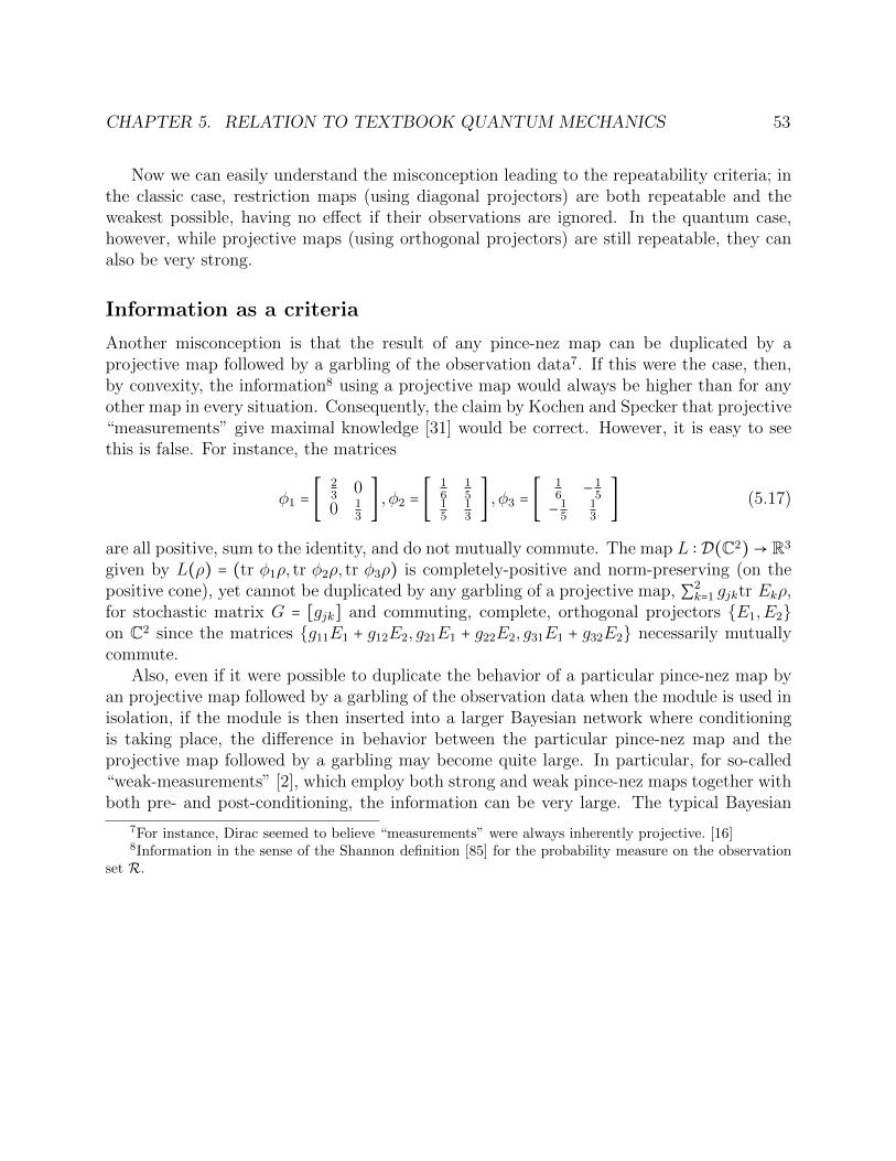
CHAPTER 5. RELATION TO TEXTBOOK QUANTUM MECHANICS 53
Now we can easily understand the misconception leading to the repeatability criteria; inthe classic case, restriction maps (using diagonal projectors) are both repeatable and theweakest possible, having no effect if their observations are ignored. In the quantum case,however, while projective maps (using orthogonal projectors) are still repeatable, they canalso be very strong.
Information as a criteria
Another misconception is that the result of any pince-nez map can be duplicated by aprojective map followed by a garbling of the observation data7. If this were the case, then,by convexity, the information8 using a projective map would always be higher than for anyother map in every situation. Consequently, the claim by Kochen and Specker that projective“measurements” give maximal knowledge [31] would be correct. However, it is easy to seethis is false. For instance, the matrices
φ1 = [23 00 1
3
] , φ2 = [16
15
15
13
] , φ3 = [16 −1
5
−15
13
] (5.17)
are all positive, sum to the identity, and do not mutually commute. The map L ∶ D(C2)→ R3
given by L(ρ) = (tr φ1ρ, tr φ2ρ, tr φ3ρ) is completely-positive and norm-preserving (on thepositive cone), yet cannot be duplicated by any garbling of a projective map, ∑2
k=1 gjktr Ekρ,for stochastic matrix G = [gjk] and commuting, complete, orthogonal projectors E1,E2on C2 since the matrices g11E1 + g12E2, g21E1 + g22E2, g31E1 + g32E2 necessarily mutuallycommute.
Also, even if it were possible to duplicate the behavior of a particular pince-nez map byan projective map followed by a garbling of the observation data when the module is used inisolation, if the module is then inserted into a larger Bayesian network where conditioningis taking place, the difference in behavior between the particular pince-nez map and theprojective map followed by a garbling may become quite large. In particular, for so-called“weak-measurements” [2], which employ both strong and weak pince-nez maps together withboth pre- and post-conditioning, the information can be very large. The typical Bayesian
7For instance, Dirac seemed to believe “measurements” were always inherently projective. [16]8Information in the sense of the Shannon definition [85] for the probability measure on the observation
set R.
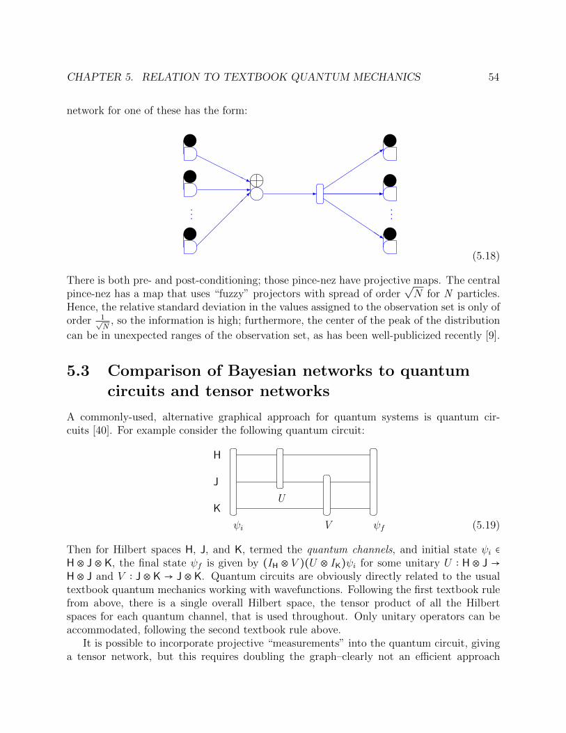
CHAPTER 5. RELATION TO TEXTBOOK QUANTUM MECHANICS 54
network for one of these has the form:
m
...
m
...
- - -
HHHHHHj
-3
QQQQQQQs
(5.18)
There is both pre- and post-conditioning; those pince-nez have projective maps. The centralpince-nez has a map that uses “fuzzy” projectors with spread of order
√N for N particles.
Hence, the relative standard deviation in the values assigned to the observation set is only oforder 1√
N, so the information is high; furthermore, the center of the peak of the distribution
can be in unexpected ranges of the observation set, as has been well-publicized recently [9].
5.3 Comparison of Bayesian networks to quantum
circuits and tensor networks
A commonly-used, alternative graphical approach for quantum systems is quantum cir-cuits [40]. For example consider the following quantum circuit:
ψi
U
V ψf
K
J
H
(5.19)
Then for Hilbert spaces H, J, and K, termed the quantum channels, and initial state ψi ∈H ⊗ J ⊗ K, the final state ψf is given by (IH ⊗ V )(U ⊗ IK)ψi for some unitary U ∶ H ⊗ J →H ⊗ J and V ∶ J ⊗ K → J ⊗ K. Quantum circuits are obviously directly related to the usualtextbook quantum mechanics working with wavefunctions. Following the first textbook rulefrom above, there is a single overall Hilbert space, the tensor product of all the Hilbertspaces for each quantum channel, that is used throughout. Only unitary operators can beaccommodated, following the second textbook rule above.
It is possible to incorporate projective “measurements” into the quantum circuit, givinga tensor network, but this requires doubling the graph–clearly not an efficient approach

CHAPTER 5. RELATION TO TEXTBOOK QUANTUM MECHANICS 55
graphically. For instance, suppose the initial state is a product state, ψi = ψ1 ⊗ ψ2 ⊗ ψ3
and that a projective “measurement” is made on the final state, where the projector is ofthe form IH ⊗ P . Then the calculation of the probability ∥IH ⊗ Pψf∥2 = ⟨IH ⊗ Pψf , ψf ⟩ isrepresented by the tensor network
fff
fffU
V P V *
U *ψ3
ψ2
ψ1
ψ∗3
ψ∗2
ψ∗1
(5.20)
The tensor network has some of the advantages of the Baysian network in that once it is setup, it is possible to look for computational shortcuts.
On the other hand, the Bayesian network has many advantages. It does not dependon the incomprehensible and unmotivated textbook rules, but instead stands on its ownreasonable basis. It is graphically more efficient in not having to duplicate itself to includeobservations. It is also potentially more efficient in allowing non-unitary nodes and non-projective pince-nez, hence avoiding the need to introduce auxiliary spaces, and in having thesplitter construction, so it is not necessary to maintain all the quantum circuits throughoutthe diagram. The Bayesian network indicates which observable nodes are being marginalizedor conditioned on and works seamlessly with the usual observable Bayesian networks thatare already in common use, so it easily allows models with information coming from previousobservations or random factors (such as coin flips). For instance, a tensor network comingfrom a quantum circuit for the “weak measurement” example (5.18) would be far morecomplicated, with the need for auxiliary spaces, yet would still not be able to indicate thepost-conditioning graphically (the pre-conditioning could be incorporated into the initialvalues for the wavefunction).
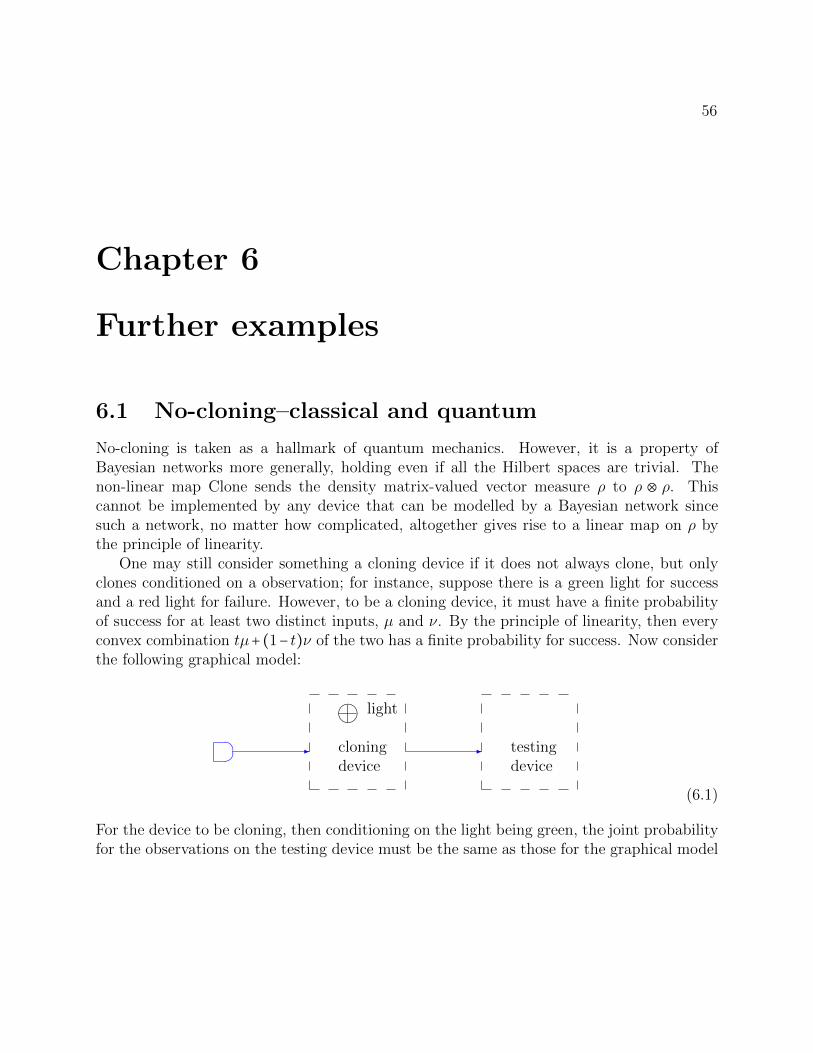
56
Chapter 6
Further examples
6.1 No-cloning–classical and quantum
No-cloning is taken as a hallmark of quantum mechanics. However, it is a property ofBayesian networks more generally, holding even if all the Hilbert spaces are trivial. Thenon-linear map Clone sends the density matrix-valued vector measure ρ to ρ ⊗ ρ. Thiscannot be implemented by any device that can be modelled by a Bayesian network sincesuch a network, no matter how complicated, altogether gives rise to a linear map on ρ bythe principle of linearity.
One may still consider something a cloning device if it does not always clone, but onlyclones conditioned on a observation; for instance, suppose there is a green light for successand a red light for failure. However, to be a cloning device, it must have a finite probabilityof success for at least two distinct inputs, µ and ν. By the principle of linearity, then everyconvex combination tµ+(1− t)ν of the two has a finite probability for success. Now considerthe following graphical model:
- -cloningdevice
testingdevice
mlight
(6.1)
For the device to be cloning, then conditioning on the light being green, the joint probabilityfor the observations on the testing device must be the same as those for the graphical model

CHAPTER 6. FURTHER EXAMPLES 57
with the Clone map
- -Clone testingdevice
(6.2)
with the same corresponding data for the testing device for each model. For every possibilityof what is put in the dashed boxes and what the corresponding information is, there are somelinear maps L from D(H)-valued vector measures on X to D(H⊗H)-valued vector measureson X ×X and K, M from the latter space to [0,1] such that the joint probability (conditioning
on the light being green) using the purported cloning device is(K L)ρ(M L)ρ , whereas the joint
probability using the mathematical Clone map is KClone(ρ) = K(ρ × ρ). With the aboveassumption, (M L)(tµ + (1 − t)ν)) ≠ 0; however, then we must have
(M L)(tµ + (1 − t)ν)K((tµ + (1 − t)ν) × (tµ + (1 − t)ν)) = (K L)(tµ + (1 − t)ν) (6.3)
for all t ∈ [0,1], which is impossible.
6.2 Teleportation-classical and quantum
Teleportation is also generally taken as a hallmark of quantum mechanics. However, as willbe shown, teleportation is also possible in classical hidden models.
A device is a teleportation device if, when modelled by a Bayesian network, for a fixed setX , base measure µ, Hilbert space H, and template density-matrix-valued function σ ∈ L1(X ×X ;µ×µ;D(H⊗H)+), it takes the product function ρ⊗σ ∈ L1(X ×X ×X ;µ×µ×µ;D(H⊗H⊗H)+)back to ρ for any ρ ∈ L1(X ;µ;D(H)+) and where a splitter is used so only Alice gets the(X , µ,H) that ρ lives on, Bob gets the final ρ, and there are no hidden connections betweenAlice and Bob, but only classic, observable information. Note that because the first textbookrule that the overall Hilbert space is the same throughout is unnecessary for the Bayesiannetwork formulation, there is no need to have another output from Alice (whose value isirrelevant in the context of being a teleportation device)–this leads to simplification in therequired calculations.
There is a Bayesian network for such a device using quantum nodes (based on, butextending, the calculations of Bennett, Brassard, Crepeau, Josza, Peres, and Wootters [5])if X = 1,2, . . . ,m, µ is the counting measure, H is Cn, and σ is the density-matrix-valued
function (written as a column vector with m2 entries, each a n2 × n2-matrix)1
mVec Im ⊗
( 1
nVec In ( Vec In)T). Note σ is the Kronecker product of Copy applied to the uniform

CHAPTER 6. FURTHER EXAMPLES 58
distribution with the usual maximally-entangled state. The graphical model is:
:
XXXXXXz
m
QQQQQQQQQQQs
*
1
2
4
5
3
m
m
@@@@@@@R
@@@@@@@
?
Alice
Bobteleportation
device(6.4)
The double arrow indicates Bob’s observations are identical to Alice’s (perfect communica-tion). The information presented in the form according to the graphical model is:
node 1 (;1,2, . . . ,m, countingmeasure
,Cn;L1) where L1 is the constant map with value ρ.
node 2 (;1,2, . . . ,m × 1,2, . . . ,m, countingmeasure
,Cn ⊗Cn;L2) where L2 is the constant
map with value σ.
splitter 3 (1,2, . . . ,m×3,countingmeasure
,Cn3;
1,2, . . . ,m × 1,2, . . . ,m, countingmeasure
,Cn ⊗Cn,1,2, . . . ,m, countingmeasure
,Cn)
pince-nez 4 (1,2, . . . ,m × 1,2, . . . ,m, countingmeasure
,Cn ⊗Cn;
1,2, . . . ,m × 1,2, . . . , n × 1,2, . . . , n, countingmeasure
; ;L4)
Let Ω be the n × n-matrix with the nth roots of unity along its diagonal, S be the n × n-shift-matrix with a one in the upper-right corner and ones on the subdiagonal, and Q bethe m ×m-shift-matrix with a one in the upper-right corner and ones on the subdiagonal.For k, l ∈ 1,2, . . . , n, let wkl be the column vector (In ⊗ (Ωl−1Sk−1)) Vec In. Then for(j, k, l) ∈ 1,2, . . . ,m × 1,2, . . . , n × 1,2, . . . , n, L4(τ)jkl is given by
( Vec Qj−1)T ((Im2 ⊗w∗kl)τ(Im2 ⊗wkl)) (6.5)

CHAPTER 6. FURTHER EXAMPLES 59
node 5 (1,2, . . . ,m × 1,2, . . . ,m × 1,2, . . . , n × 1,2, . . . , n, countingmeasure
,Cn;
1,2, . . . ,m, countingmeasure,
Cn;L5)
The incoming density-matrix-valued function τ will be considered as a m×n×n-array, indexedby j, k, l, of column vectors of m entries each, where each entry is a n×n-matrix. With thisconvention, L5(τ) is given by
m
∑j=1
n
∑k,l=1
((Qj−1)T ⊗ In) ((Im ⊗ (Ωl−1(Sk−1)T))τjkl(Im ⊗ (Sk−1Ωl−1)) (6.6)
Then, for any following testing device, the incoming density-matrix-valued function fromBob if Alice observes (j, k, l) ∈ 1,2, . . . ,m × 1,2, . . . , n × 1,2, . . . , n is
L5 (((L4 ⊗ IB(L1(X ;µ;H))))(L1 ⊗L2))∣j,k,l 1(j,k,l)) (6.7)
This apparently complicated expression is just ρ, regardless of which particular values ofj, k, l were observed by Alice and sent to Bob.
The classical case
Note the preceding is meaningful for the case of trivial Hilbert space, n = 1, so teleportationis not a quantum phenomenon. Another way to achieve the same output in this purely-classical case is to not have a template shared by Alice and Bob, but rather to have thepince-nez for Alice have simply the identity for its map (so the hidden node is not reallyhidden, but is actually observable). Then Alice sends her information to Bob, who makesa copy using the information. Finally, Alice and Bob forget what the information was (sotheir nodes are marginalized). The result is that the incoming probability distribution toAlice is the same as that outgoing from Bob.
However, this second approach is not teleportation because of the forgetting step. Also,for the classical case of the teleportation given above, an eavesdropper to the informationsent from Alice to Bob without access to the template cannot replicate the probabilitydistribution, whereas in the second, non-teleportation approach, the eavesdropper could notonly replicate the probability distribution by making his own copy, then forgetting, but bynot forgetting, would actually have more information.
Does a teleportation device really teleport?
Note the graphical model for the teleportation device is simply a graph fragment since theoutput from Bob is not terminated. One may hope its behavior is universal, but is always

CHAPTER 6. FURTHER EXAMPLES 60
possible that additional testing will reveal it is not. For instance, before the discoveryof quantum mechanics, it may have been believed that the classical teleportation discussedabove was “true” teleportation. It is possible that additional mathematical structures besidesmeasures and density matrices (see §3.8 above) can be used to calculate probabilities inBayesian networks and that these are found to be useful in practice–then the current beliefthat quantum telportation is “true” teleportation will also be shown false.
6.3 Bell’s inequality for Bayesian networks without
metaphysical limitations
Introduction
The standard proofs of Bell’s inequality [4] make assumptions based on assuming the un-derlying reality of hidden variables, which in our language is equivalent to the existence oftransition probability function. As we explored in §2.2, this is a metaphysical notion forhidden nodes. For our Bayesian networks, no such limitation is placed, which enlarges thespace of possible maps that can be employed. Although, as we already mentioned in §2.2,these additional maps are not necessarily of great interest, we would like to show that Bell’sinequality still necessarily holds.
Set-up
Following Clauser, Horne, Shimony, and Holt [11], consider the case of two observers, Aliceand Bob, who are at distant locations. Each has a box, connected by a long cable to theother, with a dial and two lights, marked zero and one, which light periodically. Theyrecord their observations, then come together later to compare notes. They find that theflashes are independent in time and depend on the settings of the dial, α for Alice and β forBob, but for each round the lights they each saw were not independent of each other, buthad a joint probability distribution given by the four functions of α,β: Prob ((0,0)∣α,β),Prob ((0,1)∣α,β), Prob ((1,0)∣α,β), and Prob ((1,1)∣α,β). Presenting the information inthis manner corresponds to the graphical model:
mBBBBBBBm
hhheeeeeee
Alice
Bob
α
β (6.8)

CHAPTER 6. FURTHER EXAMPLES 61
There are the additional no-signalling constraints on the probabilities arising from relativity:
Prob ((0,0)∣α,β) +Prob ((0,1)∣α,β) is independent of β (6.9)
Prob ((1,0)∣α,β) +Prob ((1,1)∣α,β) is independent of β
Prob ((0,0)∣α,β) +Prob ((1,0)∣α,β) is independent of α
Prob ((0,1)∣α,β) +Prob ((1,1)∣α,β) is independent of α
If these constraints were not met, then Alice and Bob could use their dial settings to trans-mit information superluminally. However, relativity places no additional constraint on thebounds for the value of, for α,α′ two settings of Alice’s dial and β, β′ two settings of Bob’sdial,
Prob ((0,0)∣α,β) +Prob ((1,1)∣α,β) −Prob ((0,1)∣α,β) −Prob ((1,0)∣α,β) (6.10)
+Prob ((0,0)∣α′, β) +Prob ((1,1)∣α′, β) −Prob ((0,1)∣α′, β) −Prob ((1,0)∣α′, β)+Prob ((0,0)∣α,β′) +Prob ((1,1)∣α,β′) −Prob ((0,1)∣α,β′) −Prob ((1,0)∣α,β′)−Prob ((0,0)∣α′, β) −Prob ((1,1)∣α′, β) +Prob ((0,1)∣α′, β) +Prob ((1,0)∣α′, β)
which can still achieve its bound in magnitude arising from the rules of probability, namelyfour.
The standard hidden variable approach
A sufficient way to insure the restrictions from relativity are met is to restrict the possiblegraphical model to the local model:
m
1
XXXXXXXXXXXz
m
m
-
:
Alice
Bob
α
β (6.11)
Then, if the space of values for the marginalized node is X and its probability measure is ρ,the joint probability both Alice and Bob get 1 is
∫x∈X
Prob (1 for Alice∣α,x)Prob (1 for Bob∣β,x) dρ(x) (6.12)
with the other joint probabilities given similarly. Using the standard approach for Bell’sinequality [11], it can be shown that for the combination of probabilities in (6.10), thebound on its magnitude has now been reduced to two.
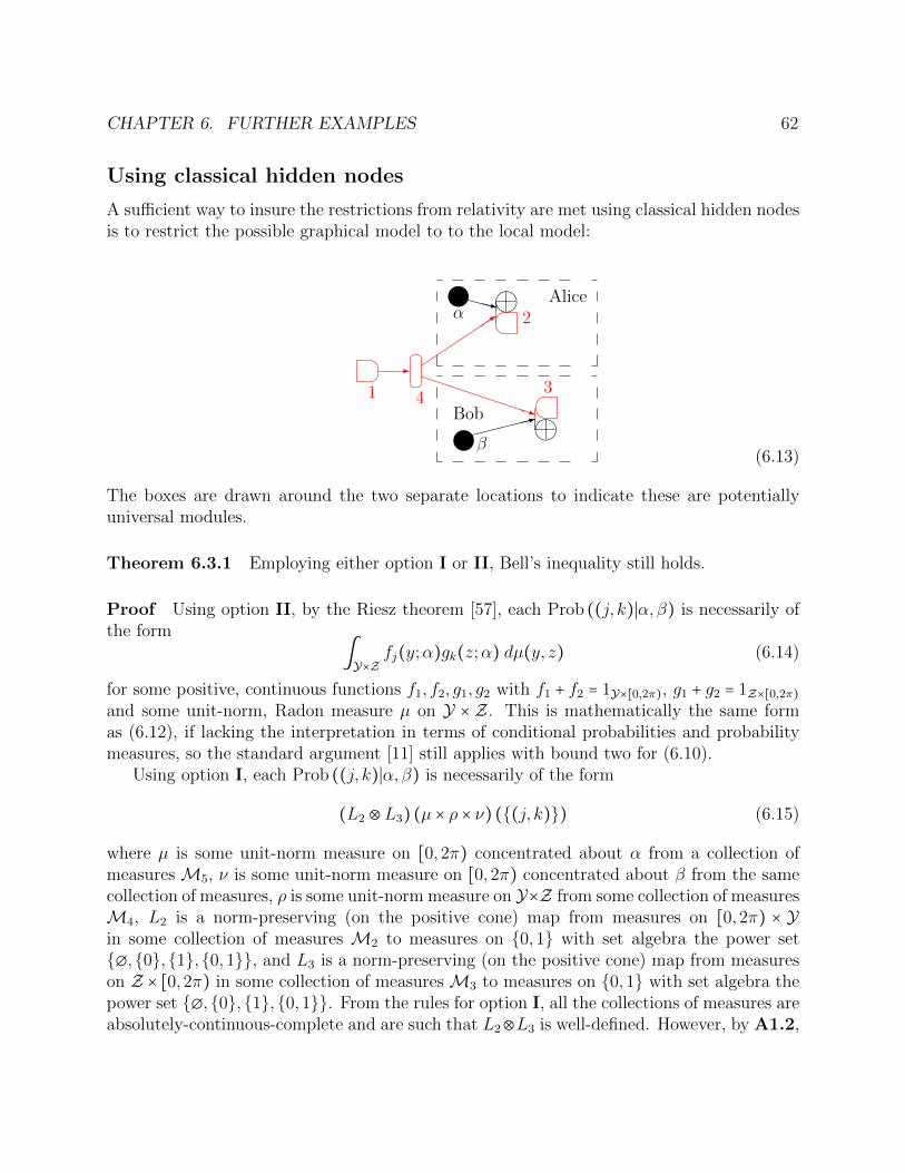
CHAPTER 6. FURTHER EXAMPLES 62
Using classical hidden nodes
A sufficient way to insure the restrictions from relativity are met using classical hidden nodesis to restrict the possible graphical model to to the local model:
- 3
PPPPPPPPq1 4
2
3
m
m
XXXz
:
Alice
Bob
α
β(6.13)
The boxes are drawn around the two separate locations to indicate these are potentiallyuniversal modules.
Theorem 6.3.1 Employing either option I or II, Bell’s inequality still holds.
Proof Using option II, by the Riesz theorem [57], each Prob ((j, k)∣α,β) is necessarily ofthe form
∫Y×Z
fj(y;α)gk(z;α) dµ(y, z) (6.14)
for some positive, continuous functions f1, f2, g1, g2 with f1 + f2 = 1Y×[0,2π), g1 + g2 = 1Z×[0,2π)and some unit-norm, Radon measure µ on Y × Z. This is mathematically the same formas (6.12), if lacking the interpretation in terms of conditional probabilities and probabilitymeasures, so the standard argument [11] still applies with bound two for (6.10).
Using option I, each Prob ((j, k)∣α,β) is necessarily of the form
(L2 ⊗L3) (µ × ρ × ν) ((j, k)) (6.15)
where µ is some unit-norm measure on [0,2π) concentrated about α from a collection ofmeasures M5, ν is some unit-norm measure on [0,2π) concentrated about β from the samecollection of measures, ρ is some unit-norm measure on Y×Z from some collection of measuresM4, L2 is a norm-preserving (on the positive cone) map from measures on [0,2π) × Yin some collection of measures M2 to measures on 0,1 with set algebra the power set∅,0,1,0,1, and L3 is a norm-preserving (on the positive cone) map from measureson Z × [0,2π) in some collection of measuresM3 to measures on 0,1 with set algebra thepower set ∅,0,1,0,1. From the rules for option I, all the collections of measures areabsolutely-continuous-complete and are such that L2⊗L3 is well-defined. However, by A1.2,
CHAPTER 6. FURTHER EXAMPLES 63
A1.3, B1.3, B1.4, and B2.5, this implies the bound can be established just be consideringProb ((j, k)∣α,β) of the form
(L2 ⊗L3)(∑l
τl × σl)((j, k)) (6.16)
where ∑l τl × σl is a unit-norm, finite-tensor-rank measure in M2 ⊗M3. Using this form forProb ((j, k)∣α,β), the usual bound of two readily follows for (6.10). ◻
Comments
Using the well-known quantum model of Clauser, Horne, Shimony, and Holt [11] (whichreuses some of the modules from the double-slit experiment (see §4.5) in a different arrangement–an example of universality), it is possible to violate Bell’s inequality and the combination ofprobabilities in (6.10) can even achieve Tsirelson’s bound of 2
√2 [10]. Any classical hidden
model duplicating these results must be nonlocal; hence, contextual–certainly the moduleswe used for the classical hidden model for the double slit experiment (see §4.7) would be ofno use.
We then have the question of whether Tsirelson’s bound can be broken. This maybe possible if there are additional mathematical structures besides measures and densitymatrices that can be utilized in Bayesian networks while respecting the principles of positivityand potential universality (see §3.8 above).
64
Part II
Parrondo’s paradox and aParrondo-like paradox
65
Chapter 7
Parrondo’s paradox
7.1 Defining the paradox
Suppose a two-player (or one-player versus the house) repeated game wins with probabilitygreater than one-half for one player as does a second repeated game. Naively, it may seemthat the convex combination of the two games using a (possibly biased) coin to determinewhich rule to employ for each round must also win for that player. However, it is possiblethat this combined game actually wins with probability greater than one-half for the secondplayer. This paradoxical result is termed Parrondo’s paradox [49].
Criteria for winning
While this paradox is displayed for several different winning criteria (see [23] for instance),here the following very simple criteria will be employed for all the following games: in total,n rounds of a game with observation set R are played. Let E be the σ-algebra of observableevents for each round. For a fixed set A ∈ E , if the state is in A at the nth round, the firstplayer (call her Alice) wins; otherwise, the second player (call him Bob) wins–regardless ofwhat was observed at the preceding rounds. (For one traditional formulation of Parrondo’sparadox, X = Z, E is its power set, and A = Z+. [49]) It is easy to see the applicability of thiscriterion for many different real-life situations–for instance, the difference of scores in sportsgames or stock options in finance.
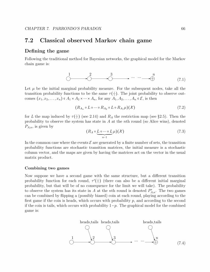
CHAPTER 7. PARRONDO’S PARADOX 66
7.2 Classical observed Markov chain game
Defining the game
Following the traditional method for Bayesian networks, the graphical model for the Markovchain game is:
k k k1 2 3- - - ⋯ ⋯ - kn
(7.1)
Let µ be the initial marginal probability measure. For the subsequent nodes, take all thetransition probability functions to be the same τ(⋅∣⋅). The joint probability to observe out-comes (x1, x2, . . . , xn) ∈ A1 ×A2 ×⋯ ×An, for any A1,A2, . . . ,An ∈ E , is then
(RAn L ⋯ RA2 L RA1µ)(X ) (7.2)
for L the map induced by τ(⋅∣⋅) (see 2.14) and RA the restriction map (see §2.5). Then theprobability to observe the system has state in A at the nth round (so Alice wins), denotedPA,n, is given by
(RA L ⋯ L´¹¹¹¹¹¹¹¹¹¹¹¹¹¹¹¸¹¹¹¹¹¹¹¹¹¹¹¹¹¹¹¹¶n−1
µ)(X ) (7.3)
In the common case where the events E are generated by a finite number of sets, the transitionprobability functions are stochastic transition matrices, the initial measure is a stochasticcolumn vector, and the maps are given by having the matrices act on the vector in the usualmatrix product.
Combining two games
Now suppose we have a second game with the same structure, but a different transitionprobability function for each round, τ ′(⋅∣⋅) (there can also be a different initial marginalprobability, but that will be of no consequence for the limit we will take). The probabilityto observe the system has its state in A at the nth round is denoted P ′
A,n. The two gamescan be combined by flipping a (possibly biased) coin at each round, playing according to thefirst game if the coin is heads, which occurs with probability p, and according to the secondif the coin is tails, which occurs with probability 1−p. The graphical model for the combinedgame is:
k k k1 2 3- - - ⋯ ⋯ - knk k kBBBBN
BBBBN
BBBBN
heads,tails heads,tails heads,tails
(7.4)
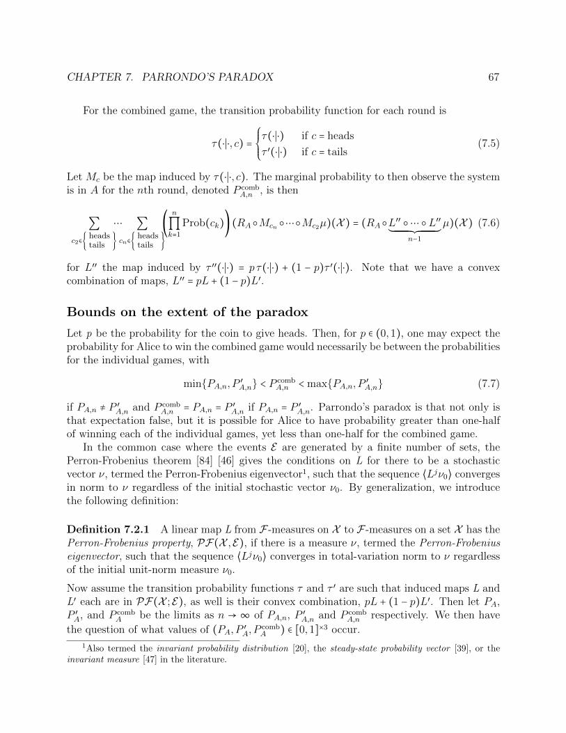
CHAPTER 7. PARRONDO’S PARADOX 67
For the combined game, the transition probability function for each round is
τ(⋅∣⋅, c) =⎧⎪⎪⎨⎪⎪⎩
τ(⋅∣⋅) if c = heads
τ ′(⋅∣⋅) if c = tails(7.5)
Let Mc be the map induced by τ(⋅∣⋅, c). The marginal probability to then observe the systemis in A for the nth round, denoted P comb
A,n , is then
∑c2∈
headstails
⋯ ∑cn∈
headstails
(n
∏k=1
Prob(ck)) (RA Mcn ⋯Mc2µ)(X ) = (RA L′′ ⋯ L′′´¹¹¹¹¹¹¹¹¹¹¹¹¹¹¹¹¹¹¹¹¹¹¹¹¸¹¹¹¹¹¹¹¹¹¹¹¹¹¹¹¹¹¹¹¹¹¹¹¹¶n−1
µ)(X ) (7.6)
for L′′ the map induced by τ ′′(⋅∣⋅) = p τ(⋅∣⋅) + (1 − p)τ ′(⋅∣⋅). Note that we have a convexcombination of maps, L′′ = pL + (1 − p)L′.
Bounds on the extent of the paradox
Let p be the probability for the coin to give heads. Then, for p ∈ (0,1), one may expect theprobability for Alice to win the combined game would necessarily be between the probabilitiesfor the individual games, with
minPA,n, P ′A,n < P comb
A,n < maxPA,n, P ′A,n (7.7)
if PA,n ≠ P ′A,n and P comb
A,n = PA,n = P ′A,n if PA,n = P ′
A,n. Parrondo’s paradox is that not only isthat expectation false, but it is possible for Alice to have probability greater than one-halfof winning each of the individual games, yet less than one-half for the combined game.
In the common case where the events E are generated by a finite number of sets, thePerron-Frobenius theorem [84] [46] gives the conditions on L for there to be a stochasticvector ν, termed the Perron-Frobenius eigenvector1, such that the sequence ⟨Ljν0⟩ convergesin norm to ν regardless of the initial stochastic vector ν0. By generalization, we introducethe following definition:
Definition 7.2.1 A linear map L from F -measures on X to F -measures on a set X has thePerron-Frobenius property, PF(X ,E), if there is a measure ν, termed the Perron-Frobeniuseigenvector, such that the sequence ⟨Ljν0⟩ converges in total-variation norm to ν regardlessof the initial unit-norm measure ν0.
Now assume the transition probability functions τ and τ ′ are such that induced maps L andL′ each are in PF(X ;E), as well is their convex combination, pL + (1 − p)L′. Then let PA,P ′A, and P comb
A be the limits as n → ∞ of PA,n, P ′A,n and P comb
A,n respectively. We then have
the question of what values of (PA, P ′A, P
combA ) ∈ [0,1]×3 occur.
1Also termed the invariant probability distribution [20], the steady-state probability vector [39], or theinvariant measure [47] in the literature.
CHAPTER 7. PARRONDO’S PARADOX 68
Definition 7.2.2 The classically allowed region, denoted C(A,X ,E , p), is the set of all(PA, P ′
A, PcombA ) ∈ [0,1]×3 that occur, for fixed A, X , E , and p, over all possible transition
probability functions τ and τ ′.
The existence of the paradox is then determined by the intersection of C with the cube(1
2 ,1] × (12 ,1] × [0, 1
2). For p = 1, P comb
A = PA and for p = 0, P combA = P ′
A; clearly no paradoxis possible. We have the following theorems for p ∈ (0,1), which indicate that there arebasically only two possibilities, depending on whether we have effectively a two-state systemor one with more than two states, as determined by the event σ-algebra E .
Theorem 7.2.3 For p ∈ (0,1), if there are nonempty, disjoint subsets A,B,C ∈ E withA ∪B ∪C = X , then C ⊃ (0,1)×3.
Proof Fix any PA, P ′A ∈ (0,1). Then take any ε > 0 sufficiently small such that both the
matrices
T =⎡⎢⎢⎢⎢⎢⎢⎣
1 − (1 − s)ε − ( 1PA
− 1 − ε) ε2 ε2 1 − s( 1PA
− 1 − ε) ε2 1 − PAsε1−(1+ε)PA
− ε2 s
(1 − s)ε PAsε1−(1+ε)PA
0
⎤⎥⎥⎥⎥⎥⎥⎦(7.8)
T′ =⎡⎢⎢⎢⎢⎢⎢⎣
1 − 1−P ′AP ′A
ε2 ε2 12
1−P ′AP ′A
ε2 1 − ε2 12
0 0 0
⎤⎥⎥⎥⎥⎥⎥⎦
are stochastic matrices for all values of s ∈ [0,1]. Take the transition probability functionsto be
⎡⎢⎢⎢⎢⎢⎣
τ(A∣x ∈ A) τ(A∣x ∈ B) τ(A∣x ∈ C)τ(B∣x ∈ A) τ(B∣x ∈ B) τ(B∣x ∈ C)τ(C ∣x ∈ A) τ(C ∣x ∈ B) τ(C ∣x ∈ C)
⎤⎥⎥⎥⎥⎥⎦= T (7.9)
⎡⎢⎢⎢⎢⎢⎣
τ ′(A∣x ∈ A) τ ′(A∣x ∈ B) τ ′(A∣x ∈ C)τ ′(B∣x ∈ A) τ ′(B∣x ∈ B) τ ′(B∣x ∈ C)τ ′(C ∣x ∈ A) τ ′(C ∣x ∈ B) τ ′(C ∣x ∈ C)
⎤⎥⎥⎥⎥⎥⎦= T′
Then the required calculations reduce to matrix products. Since the maps are assumed tohave the Perron-Frobenius property, the initial probabilities chosen for A, B, and C areirrelevant.
By the deliberate construction of T and T′, the first entry of the Perron-Frobeniuseigenvector of T is indeed PA for every s ∈ [0,1] and the first entry of the Perron-Frobeniuseigenvector of T′ is indeed P ′
A. The first entry of the Perron-Frobenius eigenvector of pT +
CHAPTER 7. PARRONDO’S PARADOX 69
(1 − p)T′, which gives P combA , varies continuously2 from
εp(1−p)
2 + ε ( pPA
+ 1−pP ′A
)= O(ε) (7.10)
to1
1 +2ε ( 1
PA− 1 − ε + εp) ( p
PA+ 1−p
P ′A− 1 − εp)
p(1 − p) + 2ε ( 1PA
− 1 − ε)
= 1 −O(ε) (7.11)
as s goes from zero to one. Since ε may be taken arbitrarily small, every value for P combA ∈
(0,1) is in the allowed region for the fixed values of PA and P ′A. ◻
Theorem 7.2.4 If E = ∅,A, A,X, then C is given by (7.7), so the paradox cannot occur.
Proof Define the stochastic matrix S by
S = [ τ(A ∣x ∈ A) τ(A ∣x ∈ A)τ(A ∣x ∈ A) τ(A ∣x ∈ A) ] (7.12)
and the stochastic matrix S′ by
S′ = [ τ′(A ∣x ∈ A) τ ′(A ∣x ∈ A)τ ′(A ∣x ∈ A) τ ′(A ∣x ∈ A) ] (7.13)
For fixed PA, P ′A ∈ (0,1], express S and S′ as
S = [ 1 − ( 1PA
− 1) ζ ζ
( 1PA
− 1) ζ 1 − ζ ] ,S′ =⎡⎢⎢⎢⎢⎣
1 − ( 1P ′A
− 1) ξ ξ
( 1P ′A
− 1) ξ 1 − ξ
⎤⎥⎥⎥⎥⎦(7.14)
for ζ ∈ (0,min PA1−PA
,1] and ξ ∈ (0,min P ′A1−P ′A
,1]. By the deliberate construction of S
and S′, the first entry of the Perron-Frobenius eigenvector of S is indeed PA for every ζand the first entry of the Perron-Frobenius eigenvector of S′ is indeed P ′
A for every ξ. ForPA ≠ P ′
A, the first entry of the Perron-Frobenius eigenvector of pS + (1 − p)S′, which givesP combA , varies continuously in the interval (minPA, P ′
A,maxPA, P ′A) as ζ, ξ vary over their
allowed values, approaching the extreme values only as either ζ or ξ go to zero since it is alinear rational function in ζ and ξ. For PA = P ′
A, P combA shares this common value for all ζ, ξ.
For PA = 0, P ′A ∈ (0,1], express S as [ 1 − ζ 0
ζ 1] for ζ ∈ (0,1] and S′ as above. Then the
first entry of the Perron-Frobenius eigenvector of S is PA = 0 for every ζ. The first entry
2The eigenvectors of a matrix are continuous functions of the entries of the matrix in any open set wherethe eigenvalues are distinct.

CHAPTER 7. PARRONDO’S PARADOX 70
of the Perron-Frobenius eigenvector of pS+ (1− p)S′, which gives P combA , varies continuously
in the interval (0, P ′A) as ζ, ξ vary over their allowed values, approaching the bounds as
either ζ or ξ go to zero. The symmetric situation holds for P ′A = 0, PA ∈ (0,1]. Finally, for
PA = P ′A = 0, express S as [ 1 − ζ 0
ζ 1] for ζ ∈ (0,1] and S′ as [ 1 − ξ 0
ξ 1] for ξ ∈ (0,1]. Then
P combA = 0 for all ζ, ξ. ◻
Understanding the cause of the paradox
While surprising when approached from the game context, mathematically the cause of theparadox is straightforward: the coefficients of the Perron-Frobenius eigenvector of a convexcombination of two matrices, M1,M2 → tM1 + (1 − t)M2, need not be in the convex hullof the coefficients of the Perron-Frobenius eigenvectors of each matrix. Large discrepanciesare possible for certain slivers of parameter values near where eigenvalues coalesce and theresulting eigenvectors are discontinuous functions of the parameters.
A similar cause is at play in the following analogous hidden classic and quantum versionsof the preceding game. In each case, there is a convex space of matrices of spectral radiusone determining the behavior of the system. A coin flip determining the rule to employ forthe next round has the effect of forming a convex combination of the matrices for each rule.In the limit as the number of rounds goes to infinity, only the eigenvector of the matrix witheigenvalue one is of importance, but the coefficients for this eigenvector are not in the convexhull of the coefficients of the eigenvectors of each matrix, leading to the paradox.
7.3 Classical hidden-Markov chain game
Defining the combined game
As will be proved below, it is possible to have Parrondo’s paradox with a game for a systemwith two states if the system is hidden. The game arises from a generalization of the ofthe commonly utilized hidden-Markov model [29] to include imagined back-reaction on thehypothesized hidden state. The standard graphical model (with hidden nodes in gray) is:
k k k k k- - - -⋯ ⋯ -
k k k k1 2 3 n
JJJJ
JJJJ
JJJJ
(7.15)
However, as has been mentioned in §2.2, this requires interpreting probabilities and/or condi-tional probabilities concerning unobservable events, which are meaningless in both Bayesianand frequentist interpretations of probability. Also, this approach has no analogy in thequantum case.

CHAPTER 7. PARRONDO’S PARADOX 71
Therefore, following the program we have laid out in the first part of this dissertation,the information for hidden nodes can simply be regarded as linear maps on measures, whichis preferable in both avoiding metaphysical notions and in having analogous meaning in thequantum case. (As has been mentioned in §2.2, this may allow additional maps which donot arise from transition probability functions, but these are not of great interest and arenot an important motivation for making the change.) Using the pince-nez construction (see§4.1), this becomes:
k k k k - - ⋯ - - -k k k k1 2 n − 1 n
(7.16)
Employing option I’ (the results can be readily recast for option II or more general forms ofoption I–see §3.2), we have the following definition:
Definition 7.3.1 A hidden-Markov-with-back-reaction-model (R, τ , H, µ, L, ν0) is com-posed of: an observation set R with base measure η, a hidden set H with base measure µ,a pince-nez map L ∈ B (L1(H;µ), L1(R ×H; η × µ)), and an initial, unit-norm measure ν0 onH that is absolutely continuous with respect to µ.
Then the joint probability to observe (x1, x2, . . . , xn) ∈ A1×A2×⋯×An, for any η-measurableA1,A2, . . . ,An, is
∫H(SAn L ⋯ SA1 L
dν0
dµ)dµ (7.17)
for SA the linear map from L1(R ×H; η × µ) to L1(H;µ) given by the partial integrationSAf = ∫A f dη. Employing this model for the game, then the marginal probability for theobservation to be in A at the nth round (so Alice wins) is
PA,n = ∫H
⎛⎜⎝SA L N ⋯ N´¹¹¹¹¹¹¹¹¹¹¹¹¹¹¹¹¹¹¹¹¸¹¹¹¹¹¹¹¹¹¹¹¹¹¹¹¹¹¹¹¹¶
n−1
dν0
dµ
⎞⎟⎠dµ (7.18)
where N ∈ B (L1(H;µ)) is defined as the map N = SR L. Because of the definition ofthe game, it is possible to reduce to the case where the event space for R is simply E =∅,A, A,X and its base measure η is the measure with η(A) = η(A) = 1.
Now suppose there is a second model with the same data except for a different pince-nezL′ for each round (it is also possible to have a different initial measure, but since the limitas n → ∞ will be taken, this is of no consequence). Once again, the two models can be

CHAPTER 7. PARRONDO’S PARADOX 72
combined by flipping a (possibly biased) coin at each round. The graphical model is:
k k k k - - -⋯ - -k k k k1 2 n − 1 n
k k k kCCCW
CCCW
CCCW
CCCW
heads,tails heads,tails heads,tails heads,tails
(7.19)
Let γ be the previously given probability measure for the coin of p for heads and 1 − p fortails, with base measure the counting measure. For simplicity of notation, we will identify γwith its Radon-Nikodym derivative dγ
dcount . For the combined game, the map for each roundis
M(f ⊗ γ) = pLf + (1 − p)L′f = L′′f (7.20)
for L′′ = pL+(1−p)L′. Let N ′,N ′′ ∈ B (L1(H;µ)) be defined using L′, L′′ as N was following(7.18), N ′ = SR L′ and N ′′ = SR L′′. Then the marginal probability for the observation tobe in A for the nth round (so Alice wins) is
P combn = ∫
HSA M (⋯(SR M ((SR M
dν0
dµ)⊗ γ))⊗ γ⋯)dµ (7.21)
= ∫H
⎛⎜⎝SA L′′ N ′′ ⋯ N ′′
´¹¹¹¹¹¹¹¹¹¹¹¹¹¹¹¹¹¹¹¹¹¹¹¹¹¹¹¹¸¹¹¹¹¹¹¹¹¹¹¹¹¹¹¹¹¹¹¹¹¹¹¹¹¹¹¹¹¶n−1
dν0
dµ
⎞⎟⎠dµ
Bounds on the extent of the paradox
One may expect the paradox to be present to an equal or greater degree for this more generalclass of games. This is indeed the case, as is seen by comparing the statements of theorem7.2.3 and 7.2.4 with the following theorem 7.3.3 and 7.3.4. Restrict the space of pince-nezmaps to those where N,N ′,N ′′ = pN + (1 − p)N ′ all have the Perron-Frobenius property,where N,N ′,N ′′ ∈ B (L1(H;µ)) are defined from L,L′, L′′ as above. Then, once again, letPA, P ′
A, and P combA be the limits as n→∞ of PA,n, P ′
A,n and P combA,n respectively.
Definition 7.3.2 The classical-hidden allowed region, denoted CH(A,R, η,H, µ, p), is theset of all (PA, P ′
A, PcombA ) ∈ [0,1]×3 that occur, for fixed A, R, τ , H, µ, and p, over all allowed
pince-nez maps L and L′.
As in the classical observed case, the existence of the paradox is then determined by theintersection of CH with the cube (1
2 ,1] × (12 ,1] × [0, 1
2). For p = 1, P comb
A = PA and for p = 0,P combA = P ′
A; clearly no paradox is possible. We have the following theorems for p ∈ (0,1),which indicate that, once again, there are basically only two possibilities, depending onwhether we have effectively a two-state hidden system or one with more than two states, asdetermined by the hidden base measure µ.

CHAPTER 7. PARRONDO’S PARADOX 73
Theorem 7.3.3 For p ∈ (0,1), if there are disjoint, µ-measurable subsets B,C,D withB ∪C ∪D = H and µ(B), µ(C), and µ(D) all strictly positive, then CH ⊃ (0,1)×3.
Proof Pick any ε > 0 and let κ be the map from L1(H;µ) to R3 given by
κ(f) =⎡⎢⎢⎢⎢⎢⎣
∫B f dµ∫C f dµ∫D f dµ
⎤⎥⎥⎥⎥⎥⎦(7.22)
Let hB, hC , and hD be unit-norm functions in L1(B;µ)+, L1(C;µ)+, and L1(D;µ)+ respec-tively, each extended to all of H by zero. Such functions certainly exist by the σ-finitenessof µ. Then define the pince-nez maps L and L′ by
Lf = 1A ⊗ ([ hB 0 0 ]Tκ(f)) + 1A ⊗ ([ 0 hC hD ]Tκ(f)) (7.23)
L′f = 1A ⊗ ([ hB 0 0 ]T′κ(f)) + 1A ⊗ ([ 0 hC hD ]T′κ(f))
for T,T′ as in theorem 7.2.3. Because of the properties of B, C, D, hB, hC , hD, and κ, therequired calculation reduces to matrix products.
Then, by the deliberate construction of the maps, the row vector
[ 1 1 1 ]T
⎡⎢⎢⎢⎢⎢⎣
1 0 00 0 00 0 0
⎤⎥⎥⎥⎥⎥⎦= [ 1 0 0 ] (7.24)
acting on the Perron-Frobenius eigenvector of T is its the first entry, which is indeed PA forevery s ∈ [0,1]. Similarly, [ 1 0 0 ]T′ acting on the Perron-Frobenius eigenvector of T′ isits first entry, which is indeed P ′
A. For the combined game, P combA is given by the row vector
[ 1 1 1 ] (pT + (1 − p)T′)⎡⎢⎢⎢⎢⎢⎣
1 0 00 0 00 0 0
⎤⎥⎥⎥⎥⎥⎦= [ 1 0 0 ] (7.25)
acting on the Perron-Frobenius eigenvector of pT + (1 − p)T′, which is once again its firstentry. As in theorem 7.2.3, this varies continuously from 0+O(ε) to 1−O(ε) as ζ goes fromzero to one. Since ε may be taken arbitrarily small, every value for P comb
A ∈ (0,1) is in theallowed region for the fixed values of PA and P ′
A. ◻
Theorem 7.3.4 For p ∈ (0,1),if the base measure µ is such that there is a µ-measurablesubset B with µ(B) and µ(B) both strictly positive, but the conditions of the precedingtheorem do not hold, then CH(p) is given by the relatively open region
minpPA, (1 − p)P ′A < P comb
A < max1 − p + pPA, p + (1 − p)P ′A

CHAPTER 7. PARRONDO’S PARADOX 74
Proof Represent measures ν on H absolutely continuous with respect to µ by column
vectors with column sum one, [ ν(B)ν(B) ]. Then all the linear maps from L1(H;µ) to L1(H;µ)
are represented by 2 × 2-matrices acting by the usual matrix product.Firstly, we will show that CH(p) contains the given region. Fix any PA, P ′
A ∈ (0,1]. Thentake any ε > 0 sufficiently small such that the matrix
N = [ 1 − ( 1PA
− 1) ε ε
( 1PA
− 1) ε 1 − ε ] (7.26)
is stochastic. Let
L = 1A ⊗ [ 1 − ( 1PA
− 1) ε 0
( 1PA
− 1) ε 0] + 1A ⊗ [ 0 ε
0 1 − ε ] (7.27)
and, for s ∈ [0,1],
N ′ = [12(1 + s) 1
2s12(1 − s) 1 − 1
2s] , L′ = P ′
A1A ⊗ N ′ + (1 − P ′A)1A ⊗N ′ (7.28)
Then [ 1 1 ]SAL = [ 1 0 ] acting on the Perron-Frobenius eigenvector of N is its first
entry, which is indeed PA by the deliberate construction of the maps. Similarly, [ 1 1 ]SA L′ = P ′
A [ 1 1 ] acting on the Perron-Frobenius eigenvector of N ′ is indeed P ′A for all s. For
the combined game, P combA is given by
[ 1 1 ]SA (pL + (1 − p)L′) = p [ 1 0 ] + (1 − p)P ′A [ 1 1 ] (7.29)
acting on the Perron-Frobenius eigenvector of pN + (1 − p)N ′. This varies continuouslyfrom (1 − p)P ′
A +O(ε) to p + (1 − p)P ′A −O(ε) as s goes from zero to one. Since ε may be
taken arbitrarily small, every value in the interval ((1 − p)P ′A, p + (1 − p)P ′
A) can be takenby P comb
A for the fixed values of PA and P ′A. Repeating the process with primed↔unprimed
and p ↔ 1 − p, every value in the interval (pPA,1 − p + pPA) can be taken by P combA for the
fixed values of PA and P ′A. A similar argument using appropriately modified maps holds for
either PA or P ′A or both of them being zero.
Now, we will show that CH(p) is contained in the given region. A key observation isthat instead of varying over all maps SA L and SA L with positive entries subject to theconstraint that N = SR L is stochastic, one may equivalently vary over all stochastic mapsN and row vectors v with entries in [0,1] (with v = [ 1 1 ]S L). The same situation
holds for the primed maps. Write v = [ a b ], N = [ 1 − c dc 1 − d ], v′ = [ a′ b′ ], and
N ′ = [ 1 − c′ d′
c′ 1 − d′ ], with a, b, c, d, a′, b′, c′, d′ ∈ [0,1] except c = d = 0, c = d = 1, c′ = d′ = 0,
and c′ = d′ = 1 are not allowed since the maps must have the Perron-Frobenius property.

CHAPTER 7. PARRONDO’S PARADOX 75
Fixing the values of PA and P ′A and using explicit expressions for the Perron-Frobenius
eigenvector gives the optimization problem:
constraints: ad + bc = PA(c + d), a′d′ + b′c′ = P ′A(c′ + d′) (7.30)
extremize: P combA = (pa + (1 − p)a′) (pd + (1 − p)d′) + (pb + (1 − p)b′) (pc + (1 − p)c′)
p(c + d) + (1 − p)(c′ + d′)The quantity to be extremized is a rational linear function of c, d, c′, d′; furthermore, theconstraints are homogeneous in the sense that they are unaffected by c→ ξc, d→ ξd for anypositive ξ and c′ → ξ′c′, d′ → ξ′d′ for any positive ξ′. Therefore, the extreme values can onlybe attained as either c, d → 0 or c′, d′ → 0. In the first case, using the remaining condition,
the quantity to be extremized is (1 − p)P ′A +
p(ad′ + bc′)(c′ + d′) . The term on the right is between
0 and p. In the second case, using the remaining condition, the quantity to be extremized is
pPA +(1 − p)(a′d + b′c)
(c + d) . The term on the right is between 0 and 1 − p. The actual extreme
values cannot be attained because the maps corresponding to those parameter values arenot allowed. ◻
7.4 Defining a quantum analogue of the Markov
model
An analogous game
As we showed in §3.3, one may consider the analogous game to the above one employingmaps on density matrices rather than maps on measures. This leads to the following Bayesiannetwork model:
Definition 7.4.1 A Markov-Bayesian-quantum model (R, η, H, L, ρ0) is composed of: anobservation set R with base measure η, a Hilbert space H, a pince-nez mapL ∈ B (D(H), L1(R; η;D(H))) that is norm-preserving (on the positive cone) and completely-positive, and an initial density-matrix ρ0 on H with tr ρ0 = 1.
The use of the word quantum will be justified below. The accompanying graphical model is(note it is the same as (7.16), illustrating the analogy graphically):
k k k k - - ⋯ - - -k k k k1 2 n − 1 n
(7.31)
Then the joint probability to observe (x1, x2, . . . , xn) ∈ A1×A2×⋯×An, for any η-measurableA1,A2, . . . ,An ∈R, is (compare to (7.17))
tr SAn L ⋯ SA1 Lρ0 (7.32)
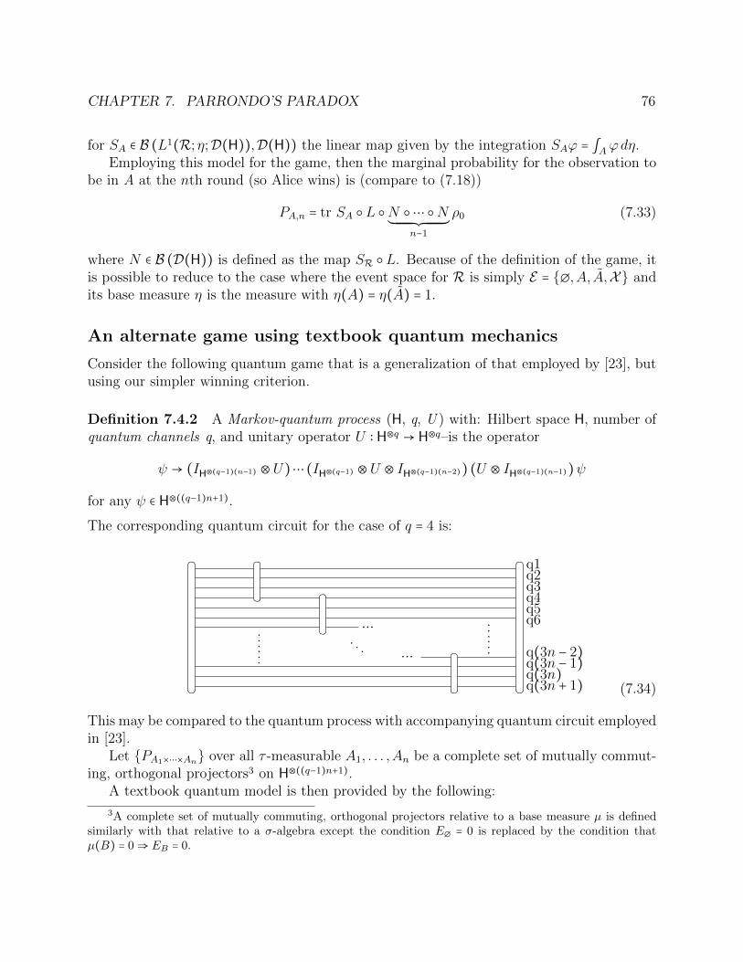
CHAPTER 7. PARRONDO’S PARADOX 76
for SA ∈ B (L1(R; η;D(H)),D(H)) the linear map given by the integration SAϕ = ∫Aϕdη.Employing this model for the game, then the marginal probability for the observation to
be in A at the nth round (so Alice wins) is (compare to (7.18))
PA,n = tr SA L N ⋯ N´¹¹¹¹¹¹¹¹¹¹¹¹¹¹¹¹¹¹¹¹¸¹¹¹¹¹¹¹¹¹¹¹¹¹¹¹¹¹¹¹¹¶n−1
ρ0 (7.33)
where N ∈ B (D(H)) is defined as the map SR L. Because of the definition of the game, itis possible to reduce to the case where the event space for R is simply E = ∅,A, A,X andits base measure η is the measure with η(A) = η(A) = 1.
An alternate game using textbook quantum mechanics
Consider the following quantum game that is a generalization of that employed by [23], butusing our simpler winning criterion.
Definition 7.4.2 A Markov-quantum process (H, q, U ) with: Hilbert space H, number ofquantum channels q, and unitary operator U ∶ H⊗q → H⊗q–is the operator
ψ → (IH⊗(q−1)(n−1) ⊗U)⋯ (IH⊗(q−1) ⊗U ⊗ IH⊗(q−1)(n−2)) (U ⊗ IH⊗(q−1)(n−1))ψ
for any ψ ∈ H⊗((q−1)n+1).
The corresponding quantum circuit for the case of q = 4 is:
......
. . . ⋯
⋯ ......
q1q2q3q4q5q6
q(3n − 2)q(3n − 1)q(3n)q(3n + 1) (7.34)
This may be compared to the quantum process with accompanying quantum circuit employedin [23].
Let PA1×⋯×An over all τ -measurable A1, . . . ,An be a complete set of mutually commut-ing, orthogonal projectors3 on H⊗((q−1)n+1).
A textbook quantum model is then provided by the following:
3A complete set of mutually commuting, orthogonal projectors relative to a base measure µ is definedsimilarly with that relative to a σ-algebra except the condition E∅ = 0 is replaced by the condition thatµ(B) = 0⇒ EB = 0.
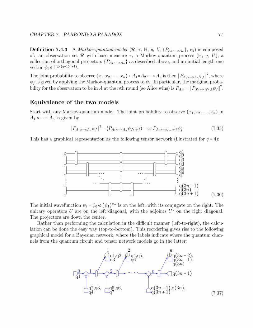
CHAPTER 7. PARRONDO’S PARADOX 77
Definition 7.4.3 A Markov-quantum-model (R, τ , H, q, U, PA1×⋯×An, ψi) is composedof: an observation set R with base measure τ , a Markov-quantum process (H, q, U ), acollection of orthogonal projectors PA1×⋯×An as described above, and an initial length-onevector ψi ∈ H⊗((q−1)n+1).
The joint probability to observe (x1, x2, . . . , xn) ∈ A1×A2×⋯×An is then ∥PA1×⋯×Anψf∥2, where
ψf is given by applying the Markov-quantum process to ψi. In particular, the marginal proba-
bility for the observation to be in A at the nth round (so Alice wins) is PA,n = ∥PX×⋯×X×Aψf∥2.
Equivalence of the two models
Start with any Markov-quantum model. The joint probability to observe (x1, x2, . . . , xn) inA1 ×⋯ ×An is given by
∥PA1×⋯×Anψf∥2 = ⟨PA1×⋯×Anψf , ψf ⟩ = tr PA1×⋯×Anψfψ
∗f (7.35)
This has a graphical representation as the following tensor network (illustrated for q = 4):
d
d
. . . . . .
. . . . . ....
...
.... . . . ..
q1q2q3q4q5q6q7
q(3n − 1)q(3n)q(3n + 1) (7.36)
The initial wavefunction ψi = ψ0 ⊗ (ψ1)⊗n is on the left, with its conjugate on the right. Theunitary operators U are on the left diagonal, with the adjoints U∗ on the right diagonal.The projectors are down the center.
Rather than performing the calculation in the difficult manner (left-to-right), the calcu-lation can be done the easy way (top-to-bottom). This reordering gives rise to the followinggraphical model for a Bayesian network, where the labels indicate where the quantum chan-nels from the quantum circuit and tensor network models go in the latter:
i i i
- - -
- -
- -
6 6 6
⋯ ⋯0 1 2 n-
i i i1 2 n
q1
q2,q3,q4
q5,q6,q7
q(3n − 1),q(3n),q(3n + 1)
q1,q2,q3
q4,q5,q6
q(3n − 2),q(3n − 1),q(3n)
q(3n + 1)
n
(7.37)
CHAPTER 7. PARRONDO’S PARADOX 78
By replacing each repeated module by a pince-nez, this becomes (7.31). (Note the efficiencyof the graphical model for the Bayesian network compared to the tensor network–there isno need to place every operator and initial condition twice in the graph.) The precedinggraphical manipulation inspires the following:
Theorem 7.4.4 If a Markov-quantum model is of the form
(R, τ,H, q,U,QA1 ⊗⋯⊗QAn ⊗ IH, ψ0 ⊗ (ψ⊗n1 ))
for some unit-length vectors ψ0 ∈ H and ψ1 ∈ H⊗(q−1) and collection of orthogonal projec-tors QCC∈E on H⊗(q−1), then there is an equivalent (in the sense of giving the same jointprobabilities) Markov-Bayesian-quantum model (R, τ , H, L, ρ0).
Proof Start with any such Markov-quantum model. The joint probability to observe(x1, x2, . . . , xn) in A1 ×⋯ ×An is given by
∥PA1×⋯×Anψf∥2 = ⟨PA1×⋯×Anψf , ψf ⟩ = tr PA1×⋯×Anψfψ
∗f (7.38)
Write the trace as the tensor product of reduced traces,
trH⊗((q−1)n+1) = (trH⊗(q−1))⊗n ⊗ trH (7.39)
This tensor product of maps is well-defined using A1.3, B4.1, B5.5, and B5.8. Using thegiven forms, PA1×⋯×An = QA1 ⊗⋯⊗QAn ⊗ IH and ψi = ψ0⊗ (ψ⊗n1 ), then “pushing” the partialtraces into the expression as far as possible gives the joint probability as
(K(⋅;An)⊗ trH) (U (((K(⋅;An−1)⊗ IB(H)) (⋯
(K(⋅;A2)⊗IB(H))(U(((K(⋅;A1)⊗IB(H)) (U(ψ0ψ∗0⊗(ψ1ψ∗1))U∗))⊗(ψ1ψ∗1))U∗)
⋯))⊗ (ψ1ψ∗1))U∗)
(7.40)
where IB(H) is the identity map on operators in B(H) and
K ∶ D (H⊗(q−1)) × ( τ −measurablesubsets of R )→ R (7.41)
is given by K(ρ;C) = tr QCρ. The various tensor products of maps in the expression are stillwell-defined by the above propositions. K is countably-additive in its second argument bythe countable-additivity of the projectors QC (with convergence in the weak* topology).K(⋅;C) is manifestly completely-positive for any C ∈ E . Then, by B5.5, and B5.8, ∥K(⋅;C)⊗IB(H)∥op = ∥K(⋅;C)∥op. Therefore, for any fixed ρ ∈ D (H⊗(q−1))+, K(ρ; ⋅) is a measure on R.Furthermore, this measure is clearly absolutely continuous with respect to τ since QC = 0 ifτ(C) = 0.

CHAPTER 7. PARRONDO’S PARADOX 79
Let N ∶ D (H) × E → D (H) be the map given by
MNρ;C) = (K(⋅;C)⊗ IB(H)) (U(ρ⊗ (ψ1ψ∗1))U∗) (7.42)
By the above properties of K, for any fixed ρ ∈ D (H)+, N(ρ; ⋅) is a D (H)+-valued vector mea-sure on R that is absolutely continuous with respect to τ . D (H) has the Radon-Nikodym
property, so N(ρ; ⋅) has Radon-Nikodym derivative dN(ρ;⋅)dτ ∈ L1(R; τ ;D (H)+) with the prop-
erty that N(ρ;C) = ∫CdN(ρ;⋅)dτ dτ for any τ -measurable subset C. Then define the pince-nez
map L by Lρ = dN(ρ;⋅)dτ . The required completely-positive and norm-preserving (on the posi-
tive cone) properties of L are readily demonstrated. ◻
More remarkable (and requiring theorem 5.1.1 to prove) is the following result:
Theorem 7.4.5 If a Markov-Bayesian-quantum model is of the form (R, τ , H, L, ψ0ψ∗0 ),then there is an equivalent (in the sense of giving the same joint probabilities) Markov-quantum-model
(R′, τ ′,H, q,U,PA1×⋯×An, ψi)
Proof Start with any such Markov-Bayesian-quantum model. From theorem 5.1.1 andthe Radon-Nikodym property of D(H), L can be written in terms of the Radon-Nikodym
derivative, Lρ = dN(ρ;⋅)dτ , with
N(ρ;B) = (trK ⊗ P (B)⊗ IB(H)) (V ρV ∗) (7.43)
for some Hilbert space K, some partial isometry V ∶ L2(H → K ⊗ L2(R; τ) ⊗ H, and whereP (B) is the functional on D(L2(R; τ)) given by P (B)τ = ∫x∈B τ(x,x) dν(x). Furthermore,by the theorem, if all the Hilbert spaces have finite dimension, the dimension of K less thanor equal to (dimH)2.
The dimension of L2(R; τ) then determines the minimum number of quantum channels,q. If dimL2(R; τ) ≤ (dimH), take q = 4. If dimH < dimL2(R; τ) ≤ (dimH)2, take q = 5.If (dimH)2 < dimL2(R; τ) ≤ (dimH)3, take q = 6. For any of these three cases, take Qto be any partial isometry from L2(R; τ) to H⊗(q−3). For (dimH)3 < dimL2(R; τ), let Gbe the subspace of L2(R; τ) which is relevant, given by the norm-closure of the span of(ψ∗ ⊗ π(1)⊗ ξ∗)V φ ∣φ,ψ ∈ H, ξ ∈ K. Then dimG ≤ (dimH)2 dimK ≤ (dimH)4, so take q = 7and Q to be any partial isometry from G to H⊗4.
Now select any unit-length ψ1 ∈ H⊗(q−1) and any partial isometry R ∶ K → H ⊗ H. Thenthere is some unitary U ∶ H⊗q → H⊗q such that
U(φ⊗ ψ1) = (R⊗Q⊗ IH)V φ for every φ ∈ H (7.44)
Hence, by the spectral theorem for compact operators,
U(ρ⊗ ψ1ψ∗1)U∗ = (R⊗Q⊗ IH)V ρV ∗(R∗ ⊗Q∗ ⊗ IH) for every ρ ∈ D(H)+ (7.45)

CHAPTER 7. PARRONDO’S PARADOX 80
Take ψi = ψ0⊗(ψ⊗n1 ). Finally, if dimL2(X ;µ) = (dimH)q−3 or dimG = (dimH)4, take X ′ = X ,τ ′ = τ , and PA1×⋯×An to be
(IH⊗2⊗Qπ(1A1)Q∗)⊗⋯⊗ (IH⊗2⊗Qπ(1An)Q∗)⊗IH (7.46)
Otherwise, add one point x0 to X to form X ′. Add an atom of weight one at x0 to τ to formτ ′. For A1, . . . ,An ∈ E , let PA1×⋯×An be defined as above. Replacing any of the Aj’s withx0, replace Qπ(1Aj)Q∗ with IH⊗(q−3)−Q∗Q. (Note that with the given initial wavefunctionand time-evolution, the probabilities for observing x0 are all zero–it is only added so theprojectors form a complete set with PX ′×n = IH⊗((q−1)n+1 .) ◻
7.5 Parrondo’s paradox for the quantum game
Defining the combined game
As a reward for our efforts in part I and in the preceding section, we can now ignore thecomplicated Markov-quantum model and instead utilize the far simpler Markov-Bayesian-quantum model. Furthermore, since the latter model uses maps that live on a convex space,it is possible to utilize coin flips to combine two games instead of the recourse to morecomplicated alternating rules for rounds previously used by [23] [41]. This combined gamehas graphical model (note it is the same as (7.19)):
k k k k - - -⋯ - -k k k k1 2 n − 1 n
k k k kCCCW
CCCW
CCCW
CCCW
heads,tails heads,tails heads,tails heads,tails
(7.47)
Again, let γ be the previously given probability measure for the coin of p for heads and 1−pfor tails, and, for simplicity of notation, identify γ with its Radon-Nikodym derivative withrespect to the counting measure. For the combined game, the map for each round is
M(ρ⊗ γ) = pLρ + (1 − p)L′ρ = L′′ρ (7.48)
for L′′ = pL + (1 − p)L′. Let N ′,N ′′ ∈ B (D(H)) be defined using L′, L′′ as N was following(7.33),as N ′ = SR L′ and N ′′ = SR L′′. Then the marginal probability for the observationto be in A for the nth round (so Alice wins) is (compare to (7.21))
P combA,n = tr SA M (⋯ (SR M ((SR Mρ0)⊗ γ))⊗ γ⋯)dµ (7.49)
= tr SA L′′ N ′′ ⋯ N ′′
´¹¹¹¹¹¹¹¹¹¹¹¹¹¹¹¹¹¹¹¹¹¹¹¹¹¹¹¹¸¹¹¹¹¹¹¹¹¹¹¹¹¹¹¹¹¹¹¹¹¹¹¹¹¹¹¹¹¶n−1
ρ0
Because of the definition of the game, it is possible to reduce to the case where E =∅,A, A,X.
CHAPTER 7. PARRONDO’S PARADOX 81
Bounds on the paradox for the quantum game
Since it is possible to embed a classical hidden system within a quantum one (see §3.6),one may expect the paradox to be present to an equal or greater degree for these quantumgames. This is indeed the case, as is seen by comparing the statements of theorems 7.3.3and 7.3.4 with the following theorem 7.5.3 and claim 7.5.5. By analogy to definition 7.2.1,we have:
Definition 7.5.1 A linear map L from D(H)+ to D(H)+ has the quantum-Perron-Frobeniusproperty, QPF(H), if there is a density matrix ρ, termed the quantum-Perron-Frobeniuseigenvector, such that the sequence ⟨Ljρ0⟩ converges in total-variation norm to ρ regardlessof the initial unit-norm density matrix ρ0.
Restrict the space of pince-nez maps L,L′ to those where N ,N ′, and their convex combi-nation, pN + (1 − p)N ′, are all in QPF(H). Then, once again, let PA, P ′
A, and P combA be the
limits as n→∞ of PA,n, P ′A,n and P comb
A,n respectively.
Definition 7.5.2 The quantum allowed region, denoted Q(A,X ,E ,H, p), is the set of all(PA, P ′
A, PcombA ) ∈ [0,1]×3 that occur, for fixed A, X , E , H, and p, over all allowed pince-nez
maps L and L′.
As in the classical case, the existence of the paradox is then determined by the intersectionof Q with the cube (1
2 ,1] × (12 ,1] × [0, 1
2). For p = 1, P comb
A = PA and for p = 0, P combA = P ′
A;clearly no paradox is possible. We have the following theorem and claims for p ∈ (0,1), whichindicate that, once again, there are basically only two possibilities, depending on whetherwe have dimH = 2 or dimH > 2.
Theorem 7.5.3 For p ∈ (0,1), if dimH > 2, then Q ⊃ (0,1)×3.
Proof Pick any ε > 0 Let H1,H2,H3 be three non-trivial subspaces of H such that H =H1 ⊕H2 ⊕H3. Choose any density matrices ν1 ∈ D(H1)+, ν2 ∈ D(H2)+, ν3 ∈ D(H3)+ with unittrace. Let κ ∶ D(H)+ → R3 be the map
κ(ρ) =⎡⎢⎢⎢⎢⎢⎣
tr ρ∣H1
tr ρ∣H2
tr ρ∣H3
⎤⎥⎥⎥⎥⎥⎦(7.50)
and define the pince-nez maps L and L′ by
Lρ = 1A ⊗ [ ν1 0 0 ]Tκ(ρ) + 1A ⊗ [ 0 ν2 ν3 ]Tκ(ρ) (7.51)
L′ρ = 1A ⊗ [ ν1 0 0 ]T′κ(ρ) + 1A ⊗ [ 0 ν2 ν3 ]T′κ(ρ)
for T,T′ as in theorem 7.2.3. Because of the properties of ν1, ν2, ν3, and κ, the requiredcalculation reduces to matrix products, which then proceeds as in the proof for theorem

CHAPTER 7. PARRONDO’S PARADOX 82
7.3.3. ◻
Employing a similar construction, for dimH = 2 we have Q(p) ⊃ CH(p). We have thefollowing two claims, backed by extensive numerical calculation:
Claim 7.5.4 For any fixed p,PA, P ′A ∈ (0,1), the minimum and maximum values of P comb
A
are achieved for pince-nez maps L and L′ each of the form ρ→ 1A ⊗ JρJ∗ + 1A ⊗KρK∗.
Claim 7.5.5 For any fixed p,PA, P ′A ∈ (0,1), the minimum and maximum values of P comb
A
lie outside the bounds given in theorem 7.3.3.
Assuming the validity of the first claim, the extremizing maps can be expressed as
Lρ = 1A ⊗ [ u1 v1
u2 v2]ρ [ u1 u2
v1 v2] + 1A ⊗ [ u3 v3
u4 v4]ρ [ u3 u4
v3 v4] (7.52)
L′ρ = 1A ⊗ [ u′1 v′1u′2 v′2
]ρ [ u′1 u′2v′1 v′2
] + 1A ⊗ [ u′3 v′3u′4 v′4
]ρ [ u′3 u′4v′3 v′4
]
for ∥u∥2 = ∥v∥2 = 1, u ⊥ v except for points excluded by the requirement of the quantumPerron-Frobenius property. We are then faced by the following optimization problem, whichmay be treated numerically:
constraints: wM−1
⎡⎢⎢⎢⎢⎢⎢⎢⎣
0001
⎤⎥⎥⎥⎥⎥⎥⎥⎦
= PA, w′M′−1
⎡⎢⎢⎢⎢⎢⎢⎢⎣
0001
⎤⎥⎥⎥⎥⎥⎥⎥⎦
= P ′A (7.53)
extremize: P combA = (pw + (1 − p)w′) (pM + (1 − p)M′)−1
⎡⎢⎢⎢⎢⎢⎢⎢⎣
0001
⎤⎥⎥⎥⎥⎥⎥⎥⎦for
w = [ ∣u1∣2 + ∣u2∣2 u1v1 + u2v2 u1v1 + u2v2 ∣v1∣2 + ∣v2∣2 ] (7.54)
w′ = [ ∣u′1∣2 + ∣u′2∣2 u′1v′1 + u′2v′2 u′1v
′1 + u′2v′2 ∣v′1∣2 + ∣v′2∣2 ]
M =
⎡⎢⎢⎢⎢⎢⎢⎢⎣
∣u1∣2 + ∣u3∣2 − 1 u1v1 + u3v3 v1u1 + v3u3 ∣v1∣2 + ∣v3∣2u1u2 + u3u4 u1v2 + u3v4 − 1 v1u2 + v3u4 v1v2 + v3v4
u2u1 + u4u3 u2v1 + u4v3 v2u1 + v4u3 − 1 v2v1 + v4v3
1 0 0 1
⎤⎥⎥⎥⎥⎥⎥⎥⎦
M′ =
⎡⎢⎢⎢⎢⎢⎢⎢⎢⎣
∣u′1∣2 + ∣u′3∣2 − 1 u′1v′1 + u′3v′3 v′1u
′1 + v′3u′3 ∣v′1∣2 + ∣v′3∣2
u′1u′2 + u′3u′4 u′1v
′2 + u′3v′4 − 1 v′1u
′2 + v′3u′4 v′1v
′2 + v3v′4
u′2u′1 + u′4u′3 u′2v
′1 + u′4v′3 v′2u
′1 + v′4u′3 − 1 v′2v
′1 + v′4v′3
1 0 0 1
⎤⎥⎥⎥⎥⎥⎥⎥⎥⎦

CHAPTER 7. PARRONDO’S PARADOX 83
Graphs, for certain representative values of p, of the minimum achievable P combA given PA, P ′
A,are given in the following section.
7.6 Summary of results
In summary, for the considered classical game whose event space E is effectively three ormore states, the analogous classical hidden game whose σ-algebra F for its hidden set iseffectively three or more states, and the analogous quantum game whose Hilbert space isthree or more dimensions, we have proven there is no limitation on the probability for Aliceto win the combined game, P comb
A , given her probabilities to win the individual games, PAand P ′
A. For the classical game with two-states, E = ∅,A, A,O, we have proven the paradox
cannot occur. For the analogous classical hidden game with two-states, F = ∅,B, B,H,we have
minpPA, (1 − p)P ′A < P comb
A < max1 − p + pPA, p + (1 − p)P ′A (7.55)
where p ∈ (0,1) is the probability for the coin to land heads.The following contour plots illustrate the lower bounds on P comb
A for the two represen-tative values of p = 0.5 (the fair coin) and p = 0.1. The paradox is displayed by minimumachievable values of P comb
A being less than one-half in the region (PA, P ′A) ∈ (1
2 ,1]×(12 ,1]. For
comparison, plots of the minimum achieved P combA for the analogous quantum game whose
Hilbert space H has dimension two, which were numerically calculated from the optimizationproblem posed in (7.53), are given as well.
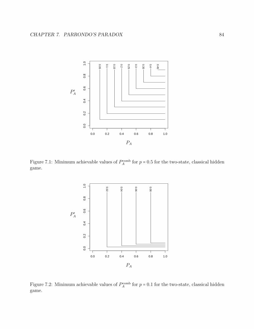
CHAPTER 7. PARRONDO’S PARADOX 84
0.05
0.1
0.15
0.2
0.25
0.3
0.35
0.4
0.45
0.0 0.2 0.4 0.6 0.8 1.0
0.0
0.2
0.4
0.6
0.8
1.0
PA
P ′A
Figure 7.1: Minimum achievable values of P combA for p = 0.5 for the two-state, classical hidden
game.
0.02
0.04
0.06
0.08
0.0 0.2 0.4 0.6 0.8 1.0
0.0
0.2
0.4
0.6
0.8
1.0
PA
P ′A
Figure 7.2: Minimum achievable values of P combA for p = 0.1 for the two-state, classical hidden
game.

CHAPTER 7. PARRONDO’S PARADOX 85
0.02
0.04
0.06
0.08
0.1
0.12 0.14 0.16
0.18
0.0 0.2 0.4 0.6 0.8 1.0
0.0
0.2
0.4
0.6
0.8
1.0
PA
P ′A
Figure 7.3: Minimum achievable values of P combA for p = 0.5 for the two-dimensional, quantum
game.
0.02
0.04
0.06
0.08
0.0 0.2 0.4 0.6 0.8 1.0
0.0
0.2
0.4
0.6
0.8
1.0
PA
P ′A
Figure 7.4: Minimum achievable values of P combA for p = 0.1 for the two-dimensional, quantum
game.

86
Chapter 8
A Parrondo-like paradox for anone-round game
8.1 Defining the game
Instead of the multi-round game considered in the preceding chapter, now consider a singleround quantum game where the winning criteria is still taken to be that the observation isin some specified set A. Instead of having two maps which are combined by a coin flip, themap is now fixed and only the initial states are varied. If they were combined in a convexcombination by flipping a coin, there would clearly be no Parrondo’s paradox since the prob-abilities depend linearly on the initial state. However, if the initial states were constrainedto be rank one (hence, described by a wavefunction), instead of a convex combination, onemay consider the minimizing geodesic joining them. If two initial states both give probabil-ity greater than one-half for the first player, Alice, to win, but there is somewhere on theminimizing geodesic where the second player, Bob, has probability greater than one-half towin, we will term that a Parrondo-like paradox.
Suppose there is a continuous control, say a slider with continuous values from zero toone, which varies the initial state along a geodesic in the space of rank-one density matrices.Using the Bayesian network model, this initial state is input into a fixed pince-nez map andthe outcome observed. The graphical model is:
- S ∈ [0,1]CCCCWk
(8.1)
Employing option I’ (see §3.2), the data for the initial node is ([0,1],Lebesgue;H;K) forsome given Hilbert space H. The map K will be determined below in §8.2. The data for thepince-nez is (H;R, τ ; ;L) for some given observable set R with base measure τ . By the rules

CHAPTER 8. A PARRONDO-LIKE PARADOX FOR AN ONE-ROUND GAME 87
of the game, it is possible to reduce to the case where the σ-algebra is ∅,A, A,R with basemeasure τ assigning both A and A the value one. Suppose L is also given.
The probability for the observation to be in set A (so Alice wins) is then
∫A(L K)ν dτ = ((L K)ν)∣A (8.2)
8.2 Defining geodesics on the space of wavefunctions
Let SH ⊂ H be the unit ball. For any ζ, η ∈ S, let ∼ be the equivalence relation ζ ∼ η if ζ = ωηfor some phase ω ∈ S1 ⊂ C and let [⋅] denote the equivalence classes. Consider a wavefunctionψ ∈ SH. Since only the rank-one density matrix ψψ∗ = ψ⟨⋅, ψ⟩ is meaningful, ψ is only definedup to an overall phase, so what should actually be considered is the equivalence class [ψ]in the quotient space SH/ ∼. The question is then what is the correct topology and metricstructure to place on this quotient space.
Choice one–using the trace norm
Using the topology and metric structure inherited from the placement of rank-one densitymatrices within all density matrices, consider the choice of metric disttrace on SH/ ∼ given by,for any [ξ], [ψ] ∈ S/ ∼,
disttrace([ξ], [ψ]) = tr ∣ξξ∗ − ψψ∗∣ = 2√
1 − ∣⟨ψ, ξ⟩∣2 (8.3)
The last equality holds since spanCξ,ψ is an invariant subspace of the operator
(ξξ∗ − ψψ∗)∗ (ξξ∗ − ψψ∗) = (ξξ∗ − ψψ∗)2(8.4)
with eigenvalue 1 − ∣⟨ψ, ξ⟩∣2 while the orthogonal subspace is the kernel of the operator.
Choice two–using the round metric on SHLet distround be the round metric on SH, which is the standard metric induced by its embed-ding in H equipped with its norm, so, for any ζ, η ∈ SH,
distround(ζ, η) = arccosR⟨ζ, η⟩ (8.5)
Then let the metric dist∼round on SH/ ∼ be given by the usual prescription for quotient spaces,so, for any [ξ], [ψ] ∈ SH/ ∼,
dist∼round([ξ], [ψ]) = minw∈S1⊂C
distround(ξ,wψ) = arccos maxw∈S1⊂C
R⟨ψ,wξ⟩ = arccos ∣⟨ψ, ξ⟩∣ (8.6)
Thendisttrace([ξ], [ψ]) = 2 sin dist∼round([ξ], [ψ]) (8.7)
⇔ dist∼round([ξ], [ψ]) = arcsin1
2disttrace([ξ], [ψ])
In particular, the metrics are equivalent and give rise to the same topology on SH/ ∼.

CHAPTER 8. A PARRONDO-LIKE PARADOX FOR AN ONE-ROUND GAME 88
Geodesics on the quotient space
Fix any ξ,ψ ∈ SH with corresponding equivalence classes [ξ], [ψ] ∈ SH/ ∼. Let ξ be anelement of [ξ] such that distround(ξ, ψ) = dist∼round([ξ], [ψ]) ⇔ ⟨ψ, ξ⟩ = ∣⟨ψ, ξ⟩∣, so ξ =⟨ψ, ξ⟩∣⟨ψ, ξ⟩∣ξ if ⟨ψ, ξ⟩ ≠ 0 while ξ can be any element of [ξ] if ⟨ψ, ξ⟩ = 0. Now take the arc
γ ∶ [0,distround(ξ, ψ)] → SH of the great circle in SH connecting ψ and ξ with the standardparametrization, given by
γ(θ) = (cos θ)ψ + (sin θ) ξ − ⟨ξ, ψ⟩ψ∥ξ − ⟨ξ, ψ⟩ψ∥
(8.8)
where ∥ξ − ⟨ξ, ψ⟩ψ∥ =√
⟨ξ − ⟨ξ, ψ⟩ψ, ξ − ⟨ξ, ψ⟩ψ⟩ =√
1 − ⟨ξ, ψ⟩2.
Proposition 8.2.1 The curve [γ] in SH/ ∼ is an unit speed geodesic with respect to themetric dist∼round.
Proof For any θ ∈ (0,distround(ξ, ψ)),
dist∼round([γ(θ)], [ψ]) + dist∼round([ξ], [γ(θ)]) = distround(γ(θ), ψ) + distround(ξ, γ(θ)) (8.9)
= distround(ξ, ψ)= dist∼round([ξ], [ψ])
so not only is the curve [γ] a geodesic, but by further partitioning, the metric is seen to beprecisely the arclength of the geodesic. Also, for any θ ∈ (0,distround(ξ, ψ)),
limε→0+
1
εdist∼round([γ(θ + ε)], [γ(θ)]) = lim
ε→0+
1
εarccos (cos(ε)) = lim
ε→0+
∣ε∣ε= 1 (8.10)
so the curve is unit speed. ◻
Proposition 8.2.2 The curve [γ] in SH/ ∼ is a geodesic with respect to the metric disttrace.
Proof Since 2 sin z = 2z + O(z3) as z → 0, the arclength of a curve with respect to themetric disttrace is simply twice the arclength with respect to the metric dist∼round. Hence, thetwo metrics have the same geodesics.◻
Completing the definition of the game.
We still need to define the initialization map K from §8.1 which uses the slider position todetermine a point on the geodesic. From the preceding results on geodesics, K is determined

CHAPTER 8. A PARRONDO-LIKE PARADOX FOR AN ONE-ROUND GAME 89
by first fixing the endpoints [ξ], [ψ] ∈ SH/ ∼. Let δ = dist∼round([ξ], [ψ]). Then, for ν ameasure on [0,1] absolutely continuous with respect to Lebesgue measure λ,
Kdν
dλ= ∫
x∈[0,1]γ(xδ)γ(xδ)∗ dν(x) (8.11)
If ν is sufficiently concentrated, then, as desired, the image of K is approximately rank-one.The complication of dealing with a concentrated measure ν for the slider position is anotherinstance of the previously mentioned problem (see §3.2 and §4.5) of inputting parametersencountered when employing option I’–the value of the slider cannot be read in directly.For purposes of simplicity and clarity, in the remainder we will instead simply suppose wecan directly select the desired point on the geodesic and work with strictly rank-one densitymatrices.
8.3 Bounds on the extent of the Parrondo-like
paradox
To quantify the extent of the Parrondo-like paradox, by analogy to §7 we have PA, P ′A, as
the probability Alice wins with initial wavefunction [ξ] and [ψ] respectively. Define P geoA
as the probability Alice wins with initial wavefunction for a specified point on the geodesicjoining [ξ] and [ψ]. Analogously to definition 7.5.2, we have the following:
Definition 8.3.1 The quantum allowed region, denoted Q(A,R, τ,H), is the set of all(PA, P ′
A, PgeoA ) ∈ [0,1]×3 that occur–for fixed A, R, τ , and H–over all allowed pince-nez maps
L, initial wavefunctions [ξ] and [ψ], and points on the geodesic joining them.
The paradox can occur if Q intersects the cube (12 ,1]× (1
2 ,1]× [0, 12). We have the following
theorem giving Q precisely:
Theorem 8.3.2 If the Hilbert space H is nontrivial, Q is the closed region
max0, PA + P ′A − 1 ≤ P geo
A ≤ minPA + P ′A,1
Proof Since the bounded operators are dual to the trace-class ones, there is some self-adjoint operator η ∈ B(H) such that L(ρ)∣A = tr ηρ for every ρ ∈ D(H)+ and, by B5.15 andB5.16, every ρ ∈ S1(H). The condition on η is that it is in the order interval 0 ≤ η ≤ IH. Letthe 2 × 2-, Hermitian matrix B = [bjk] be given by
[ L(ψψ∗)∣A L(ψξ∗)∣A
L(ξψ∗)∣A L(ξξ∗)∣A] = [ ⟨ηψ,ψ⟩ ⟨ηψ, ξ⟩
⟨ηξ, ψ⟩ ⟨ηξ, ξ⟩ ] (8.12)
Let B be the set of all such matrices over 0 ≤ η ≤ IH and ψ, ξ ∈ SH.
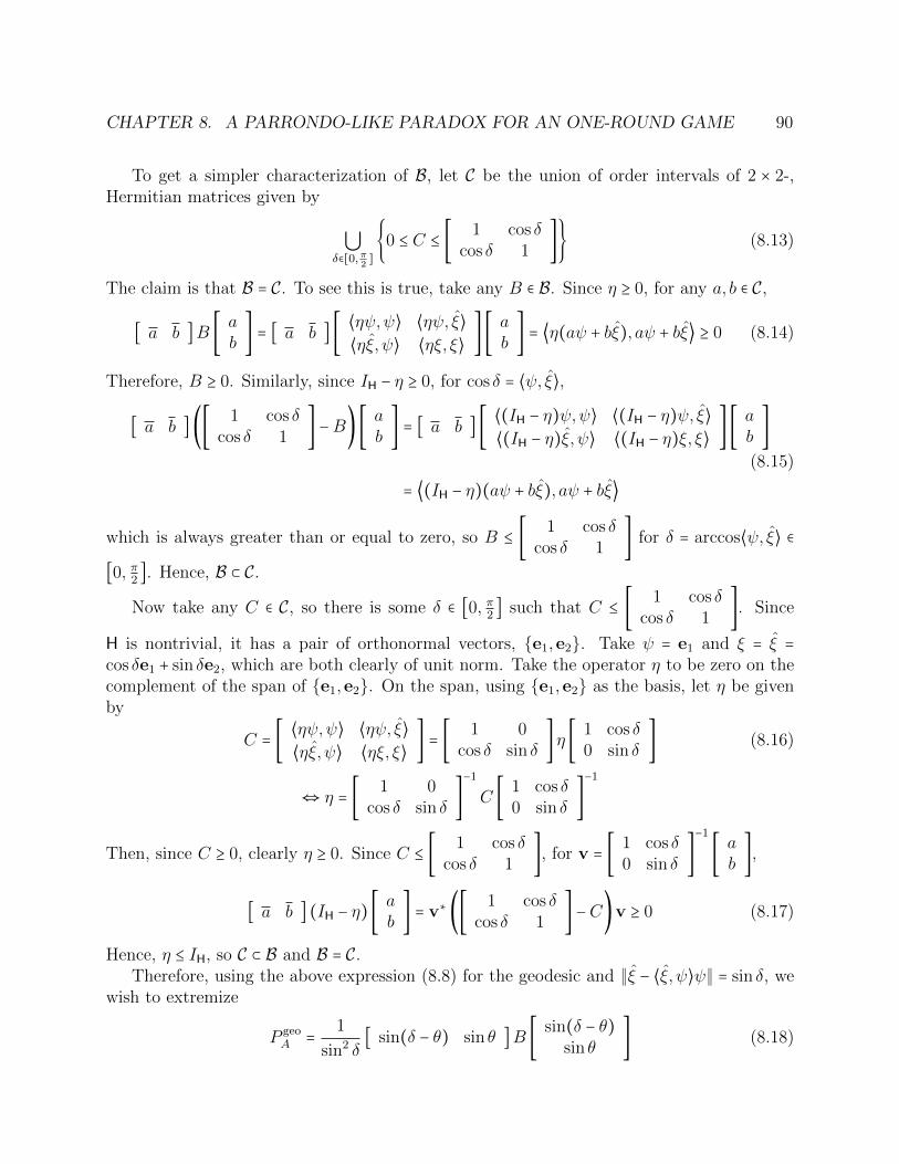
CHAPTER 8. A PARRONDO-LIKE PARADOX FOR AN ONE-ROUND GAME 90
To get a simpler characterization of B, let C be the union of order intervals of 2 × 2-,Hermitian matrices given by
⋃δ∈[0,π
2]
0 ≤ C ≤ [ 1 cos δcos δ 1
] (8.13)
The claim is that B = C. To see this is true, take any B ∈ B. Since η ≥ 0, for any a, b ∈ C,
[ a b ]B [ ab
] = [ a b ] [ ⟨ηψ,ψ⟩ ⟨ηψ, ξ⟩⟨ηξ, ψ⟩ ⟨ηξ, ξ⟩ ] [ a
b] = ⟨η(aψ + bξ), aψ + bξ⟩ ≥ 0 (8.14)
Therefore, B ≥ 0. Similarly, since IH − η ≥ 0, for cos δ = ⟨ψ, ξ⟩,
[ a b ] ([ 1 cos δcos δ 1
] −B)[ ab
] = [ a b ] [ ⟨(IH − η)ψ,ψ⟩ ⟨(IH − η)ψ, ξ⟩⟨(IH − η)ξ, ψ⟩ ⟨(IH − η)ξ, ξ⟩
] [ ab
]
(8.15)
= ⟨(IH − η)(aψ + bξ), aψ + bξ⟩
which is always greater than or equal to zero, so B ≤ [ 1 cos δcos δ 1
] for δ = arccos⟨ψ, ξ⟩ ∈
[0, π2 ]. Hence, B ⊂ C.
Now take any C ∈ C, so there is some δ ∈ [0, π2 ] such that C ≤ [ 1 cos δcos δ 1
]. Since
H is nontrivial, it has a pair of orthonormal vectors, e1,e2. Take ψ = e1 and ξ = ξ =cos δe1 + sin δe2, which are both clearly of unit norm. Take the operator η to be zero on thecomplement of the span of e1,e2. On the span, using e1,e2 as the basis, let η be givenby
C = [ ⟨ηψ,ψ⟩ ⟨ηψ, ξ⟩⟨ηξ, ψ⟩ ⟨ηξ, ξ⟩ ] = [ 1 0
cos δ sin δ] η [ 1 cos δ
0 sin δ] (8.16)
⇔ η = [ 1 0cos δ sin δ
]−1
C [ 1 cos δ0 sin δ
]−1
Then, since C ≥ 0, clearly η ≥ 0. Since C ≤ [ 1 cos δcos δ 1
], for v = [ 1 cos δ0 sin δ
]−1
[ ab
],
[ a b ] (IH − η) [ab
] = v∗ ([ 1 cos δcos δ 1
] −C)v ≥ 0 (8.17)
Hence, η ≤ IH, so C ⊂ B and B = C.Therefore, using the above expression (8.8) for the geodesic and ∥ξ − ⟨ξ, ψ⟩ψ∥ = sin δ, we
wish to extremize
P geoA = 1
sin2 δ[ sin(δ − θ) sin θ ]B [ sin(δ − θ)
sin θ] (8.18)
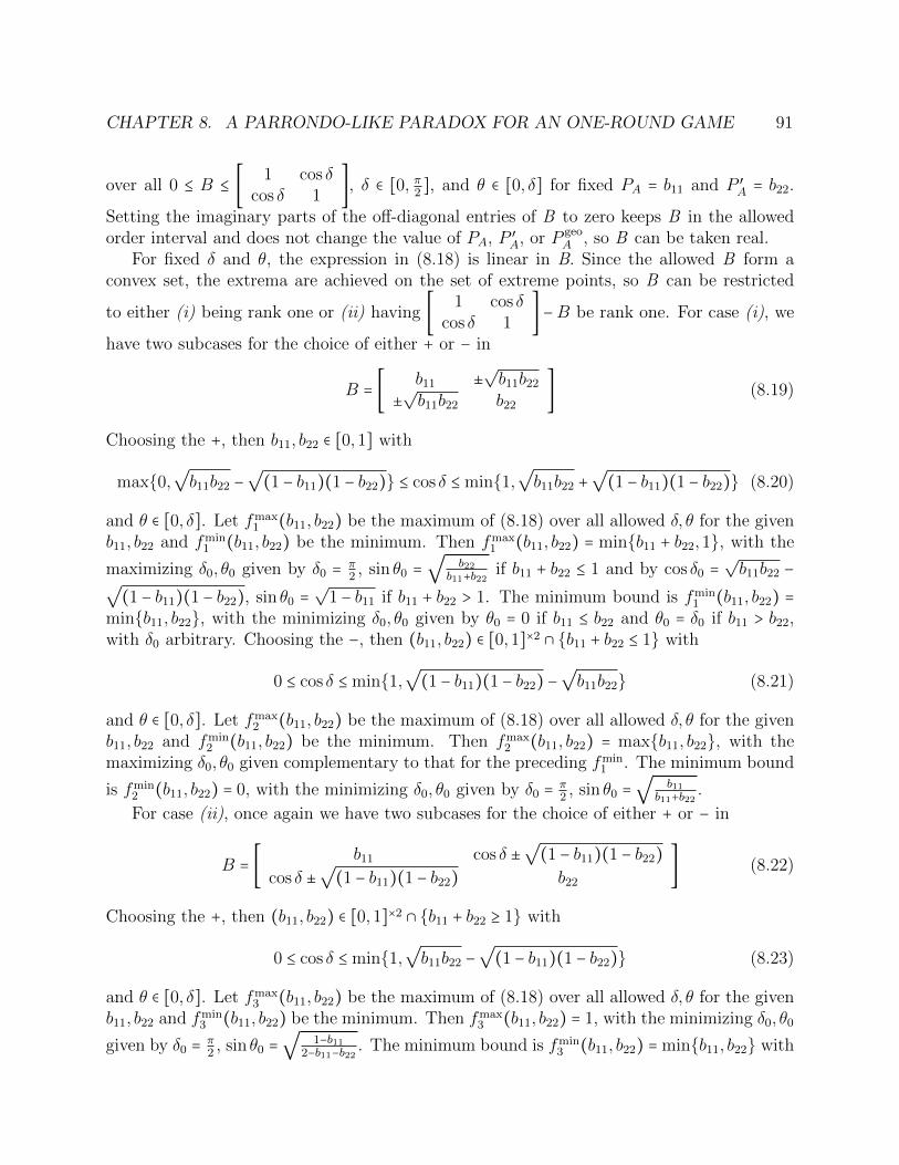
CHAPTER 8. A PARRONDO-LIKE PARADOX FOR AN ONE-ROUND GAME 91
over all 0 ≤ B ≤ [ 1 cos δcos δ 1
], δ ∈ [0, π2 ], and θ ∈ [0, δ] for fixed PA = b11 and P ′A = b22.
Setting the imaginary parts of the off-diagonal entries of B to zero keeps B in the allowedorder interval and does not change the value of PA, P ′
A, or P geoA , so B can be taken real.
For fixed δ and θ, the expression in (8.18) is linear in B. Since the allowed B form aconvex set, the extrema are achieved on the set of extreme points, so B can be restricted
to either (i) being rank one or (ii) having [ 1 cos δcos δ 1
] −B be rank one. For case (i), we
have two subcases for the choice of either + or − in
B = [ b11 ±√b11b22
±√b11b22 b22
] (8.19)
Choosing the +, then b11, b22 ∈ [0,1] with
max0,√b11b22 −
√(1 − b11)(1 − b22) ≤ cos δ ≤ min1,
√b11b22 +
√(1 − b11)(1 − b22) (8.20)
and θ ∈ [0, δ]. Let fmax1 (b11, b22) be the maximum of (8.18) over all allowed δ, θ for the given
b11, b22 and fmin1 (b11, b22) be the minimum. Then fmax
1 (b11, b22) = minb11 + b22,1, with the
maximizing δ0, θ0 given by δ0 = π2 , sin θ0 =
√b22
b11+b22if b11 + b22 ≤ 1 and by cos δ0 =
√b11b22 −√
(1 − b11)(1 − b22), sin θ0 =√
1 − b11 if b11 + b22 > 1. The minimum bound is fmin1 (b11, b22) =
minb11, b22, with the minimizing δ0, θ0 given by θ0 = 0 if b11 ≤ b22 and θ0 = δ0 if b11 > b22,with δ0 arbitrary. Choosing the −, then (b11, b22) ∈ [0,1]×2 ∩ b11 + b22 ≤ 1 with
0 ≤ cos δ ≤ min1,√
(1 − b11)(1 − b22) −√b11b22 (8.21)
and θ ∈ [0, δ]. Let fmax2 (b11, b22) be the maximum of (8.18) over all allowed δ, θ for the given
b11, b22 and fmin2 (b11, b22) be the minimum. Then fmax
2 (b11, b22) = maxb11, b22, with themaximizing δ0, θ0 given complementary to that for the preceding fmin
1 . The minimum bound
is fmin2 (b11, b22) = 0, with the minimizing δ0, θ0 given by δ0 = π
2 , sin θ0 =√
b11b11+b22
.
For case (ii), once again we have two subcases for the choice of either + or − in
B = [ b11 cos δ ±√
(1 − b11)(1 − b22)cos δ ±
√(1 − b11)(1 − b22) b22
] (8.22)
Choosing the +, then (b11, b22) ∈ [0,1]×2 ∩ b11 + b22 ≥ 1 with
0 ≤ cos δ ≤ min1,√b11b22 −
√(1 − b11)(1 − b22) (8.23)
and θ ∈ [0, δ]. Let fmax3 (b11, b22) be the maximum of (8.18) over all allowed δ, θ for the given
b11, b22 and fmin3 (b11, b22) be the minimum. Then fmax
3 (b11, b22) = 1, with the minimizing δ0, θ0
given by δ0 = π2 , sin θ0 =
√1−b11
2−b11−b22. The minimum bound is fmin
3 (b11, b22) = minb11, b22 with

CHAPTER 8. A PARRONDO-LIKE PARADOX FOR AN ONE-ROUND GAME 92
the minimizing δ0, θ0 given similarly to that for the preceding fmin1 . Choosing the −, then
b11, b22 ∈ [0,1] with
max0,√
(1 − b11)(1 − b22) −√b11b22 ≤ cos δ ≤ min1,
√(1 − b11)(1 − b22) +
√b11b22 (8.24)
and θ ∈ [0, δ]. Let fmax4 (b11, b22) be the maximum of (8.18) over all allowed δ, θ for the
given b11, b22 and fmin4 (b11, b22) be the minimum. Then fmax
4 (b11, b22) = minb11, b22 withthe maximizing δ0, θ0 given similarly to that for the preceding fmin
1 . The minimum bound isfmin
4 (b11, b22) = max0, b11 + b22 − 1, with the minimizing δ0, θ0 given by cos δ0 =√
1 − b11√1 − b22 −
√b11b22, sin θ0 =
√b11 if b11 + b22 ≤ 1 and δ0 = π
2 , sin θ0 =√
1−b222−b11−b22
if b11 + b22 > 1.
Putting the cases and subcases together, the minimum value of P geoA for fixed PA, P ′
A isgiven by
(fmin1 ∧ fmin
2 ∧ fmin3 ∧ fmin
4 ) (PA, P ′A) = fmin
4 (PA, P ′A) = max0, PA + P ′
A − 1 (8.25)
The maximum value of P geoA for fixed PA, P ′
A is given by
(fmax1 ∨ fmax
2 ∨ fmax3 ∨ fmax
4 ) (PA, P ′A) = fmax
1 (PA, P ′A) = minPA + P ′
A,1 (8.26)
With fixed values for PA and P ′A, within each case and subcase P geo
A is a continuous functionof δ and θ, so all intermediate values for P geo
A are achieved. ◻Note that, by the result of the preceding theorem, the paradox can only occur for values of(PA, P ′
A) in the triangle bounded by PA > 12 , P ′
A > 12 , and PA + P ′
A < 32 .
8.4 Conditions for the occurrence of the
Parrondo-like paradox
The matrix B defined in the proof of the preceding theorem (8.12) puts restrictions on theoccurrence of the paradox. If B ≤ 1
2I2 then both PA and P ′A are less than or equal to one-
half, so the paradox cannot occur for any choices of [ψ], [ξ], or point on the geodesic joiningthem. Similarly, if the trace of B is less than or equal to one, then either PA or P ′
A is lessthan one-half, so the paradox also cannot occur. From these obvious statements, we thenhave the following nontrivial result:
Theorem 8.4.1 If, for any particular orthonormal e1,e2 ∈ H,
tr [ L(e1e∗1)∣A L(e1e∗2)∣AL(e2e∗1)∣A L(e2e∗2)∣A
] ≤ 1
then, for any normalized ψ, ξ ∈ spanCe1,e2 and point on the geodesic joining [ψ] and [ξ],the paradox cannot occur.

CHAPTER 8. A PARRONDO-LIKE PARADOX FOR AN ONE-ROUND GAME 93
Proof Let ψ = [ e1 e2 ] [ ab
] and ξ = [ e1 e2 ] [ cd
] with ∣a∣2 + ∣b∣2 = ∣c∣2 + ∣d∣2 = 1 and
ac + bd = cos δ real and greater than or equal to zero. Let
C = [ L(e1e∗1)∣A L(e1e∗2)∣AL(e2e∗1)∣A L(e2e∗2)∣A
] (8.27)
If C ≤ 12I2, then
tr B = tr [ a b
c d]C [ a c
b d] ≤ 1 (8.28)
so, by the comment preceding the theorem, the paradox cannot occur. Therefore, the onlyremaining case is where C, whose eigenvalues are necessarily real, has one eigenvalue, λ1 > 1
2 ,and one eigenvalue, λ2 < 1
2 , with λ1+λ2 ≤ 1. There are corresponding normalized eigenvectors
v1 and v2, necessarily orthogonal. Writing [ ac
] = f1v1 + f2v2 and [ bd
] = g1v1 + g2v2, the
above conditions on a, b, c, d become the following conditions on f1, f2, g1, g2: ∣f1∣2 + ∣f2∣2 = 1,∣g1∣2 + ∣g2∣2 = 1, and f1g1 + f2g2 = cos δ is a positive real or zero.
For the paradox to occur, it must be that both ∣f1∣2λ1 + ∣f2∣2λ2 = b11 = PA > 12 and
∣g1∣2λ1 + ∣g2∣2λ2 = b22 = P ′A > 1
2 ; hence,
∣f1∣ >
¿ÁÁÀ 1
2 − λ2
λ1 − λ2
and ∣f2∣ <
¿ÁÁÀ λ1 − 1
2
λ1 − λ2
⇒ ∣f1∣ >¿ÁÁÀ
12 − λ2
λ1 − 12
∣f2∣ (8.29)
∣g1∣ >
¿ÁÁÀ 1
2 − λ2
λ1 − λ2
and ∣g2∣ <
¿ÁÁÀ λ1 − 1
2
λ1 − λ2
⇒ ∣g1∣ >¿ÁÁÀ
12 − λ2
λ1 − 12
∣g2∣ (8.30)
Then, since
∣f1g1∣ = ∣f1∣∣g1∣ >12 − λ2
λ1 − 12
∣f2∣∣g2∣ > ∣f2∣∣g2∣ = ∣f2g2∣ (8.31)
it must be that f1g1 + f2g2 is actually strictly positive and that Rf1g1 > 0. Furthermore,since the imaginary parts of f1g1 and f2g2 are equal in magnitude, it must be that the real
part of f1g1 is greater than12−λ2
λ1−12
times the magnitude of the real part of f2g2 and, therefore,
is greater than12−λ2
λ1−12
times the real part of f2g2. Hence, rearranging terms,
R (λ1f1g1 + λ2f2g2) >1
2(f1g1 + f2g2) =
1
2cos δ (8.32)
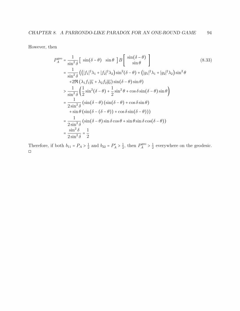
CHAPTER 8. A PARRONDO-LIKE PARADOX FOR AN ONE-ROUND GAME 94
However, then
P geoA = 1
sin2 δ[ sin(δ − θ) sin θ ]B [ sin(δ − θ)
sin θ] (8.33)
= 1
sin2 δ((∣f1∣2λ1 + ∣f2∣2λ2) sin2(δ − θ) + (∣g1∣2λ1 + ∣g2∣2λ2) sin2 θ
+2R (λ1f1g1 + λ2f2g2) sin(δ − θ) sin θ)
> 1
sin2 δ(1
2sin2(δ − θ) + 1
2sin2 θ + cos δ sin(δ − θ) sin θ)
= 1
2 sin2 δ(sin(δ − θ) (sin(δ − θ) + cos δ sin θ)
+ sin θ (sin(δ − (δ − θ)) + cos δ sin(δ − θ)))
= 1
2 sin2 δ(sin(δ − θ) sin δ cos θ + sin θ sin δ cos(δ − θ))
= sin2 δ
2 sin2 δ= 1
2
Therefore, if both b11 = PA > 12 and b22 = P ′
A > 12 , then P geo
A > 12 everywhere on the geodesic.
◻

95
Chapter 9
Quantum walks and the Parrondo-likeparadox
9.1 Classical random and classical hidden walks
Definitions of classical random and classical hidden walks
A classical random walk is a special case of the observable Markov chain earlier discussed,with graphical model given in figure (7.1). It models a walker who is in one of a finitenumber of internal states and occupies one of a countable number of positions at one time,so the space X is either J × Z+ for a walk on the half-line, or J × Z for a walk on thefull line. After each time-step, the walker is at the same or a neighboring location and itsinternal state can change as well. The process is random, with the transition probabilityfunctions possibly dependent on the internal state as well as on the location. This constrainsthe transition probability functions further than the constraints already imposed by theMarkov conditions, but these further constraints are not indicated in the graphical model.If the transition probability functions are spatially translation invariant, the walk is termedhomogeneous.
Now we may consider a classical hidden walk. This is in some ways a special caseof the classical hidden-Markov chain earlier discussed (7.16), while in other ways it is ageneralization. The hidden set H is required to be either J ×Z+ for a walk on the half-line,or J ×Z for a walk on the full line. The base measure for the hidden set is required to be thecounting measure, and L1 (H; counting measure) ≅ `1, so all integrals can be taken to just besums. The space `1 has a natural basis of sequences that have a single nonzero entry withvalue one. There is a dual “basis” of sequences in `∞ of the same sequences, which is not abasis in the norm topology, but is one in the weak* topology. This basis and dual “basis”can be used to assign matrix elements to any operator in B(`1). Then any operator, A, inB(`1) is in one-to-one correspondence to a certain sequence of matrices, An, which maybe considered the truncations of the infinite matrix corresponding to the operator. By the

CHAPTER 9. QUANTUM WALKS AND THE PARRONDO-LIKE PARADOX 96
triangle inequality, these sequences converge to the operator in the strong-operator topology:
limn→∞
∥Ax −Anx∥ = limn→∞
∥Ax − PnAPnx∥ ≤ limn→∞
(∥Ax − PnAx∥ + ∥PnAx − PnAPnx∥) (9.1)
≤ limn→∞
(∥(Ax) − Pn(Ax)∥ + ∥PnA∥op∥x − Pnx∥) = 0
for any x ∈ `1, where Pn are the usual, diagonal projectors onto the span of the first nbasis elements.
Conversely, given a sequence of matrices, each of which is the truncation of the following,the condition on the sequence so that it actually corresponds to a bounded operator is thatthe induced operator norm of all the matrices is bounded. However, the operator norminduced by the `1 norm is simply the supremum over all columns of the column sum ofthe magnitudes of the entries, so it is readily calculated. With this form for the maps, thecondition that this is a walk (rather than some other sort of hidden-Markov process) is thatmatrix entries connecting spatial locations that are not neighboring are all zero.
The generalization from the classical hidden-Markov chain is that the last pince-nez mapin the chain is no longer required to be the same as the preceding ones; in particular, all thepreceding pince-nez can be taken to be simply nodes, so the graphical model is
k k k - - -⋯ ⋯ - -
1 2 n kn + 1
(9.2)
Note there is nothing graphically that distinguishes this from a more general Markov process–the constraints that make it a walk are not represented graphically.
Connection to orthogonal polynomials and measures on ROrthogonal polynomials1 pj result from the Gram-Schmidt algorithm applied to 1, x, x2, . . .on the real line with inner-product given with respect to some Borel measure µ, ⟨f, g⟩ =∫R fg dµ. These polynomials all have the maximal number of real roots, which are all sim-ple, else they would not change signs enough times to be orthogonal. For the same reason,the roots are all within the convex hull of the support of µ and they interlace as j increasesby one. By orthogonality, the polynomials necessarily obey a three-term recurrence relation,which may be written in matrix form as
x [ p0 p1 ⋯ ] = [ p0 p1 ⋯ ]
⎡⎢⎢⎢⎢⎢⎢⎢⎢⎢⎢⎣
b0 c1
a0 b1 c2
a1
. . .. . .
. . .. . .
⎤⎥⎥⎥⎥⎥⎥⎥⎥⎥⎥⎦
(9.3)
1The following results on orthogonal polynomials are well known and included for comparison to theresults for quantum walks given below. For details, see[89].

CHAPTER 9. QUANTUM WALKS AND THE PARRONDO-LIKE PARADOX 97
If the polynomials are normalized to have value one at x = 1, the tridiagonal, infinite matrixon the right has column sum one for each of its columns. If µ is such that all the entriesin that matrix are positive, then it is a stochastic matrix and can be used for the map pertime step for a classical random or classical hidden walk on the half-line where the internalstates are trivial.
Conversely, given such a walk, then there is an infinite, stochastic matrix
⎡⎢⎢⎢⎢⎢⎢⎢⎢⎢⎢⎣
b0 c1
a0 b1 c2
a1
. . .. . .
. . .. . .
⎤⎥⎥⎥⎥⎥⎥⎥⎥⎥⎥⎦
(9.4)
giving the map per time step. If all the a’s and c’s are strictly positive, then each n × n-truncation An of the matrix is similar to a Hermitian matrix via
⎡⎢⎢⎢⎢⎢⎢⎢⎢⎢⎣
11d1
. . .1
dn−1
⎤⎥⎥⎥⎥⎥⎥⎥⎥⎥⎦
⎡⎢⎢⎢⎢⎢⎢⎢⎢⎢⎢⎢⎢⎣
b0 c1
a0 b1 c2
a1
. . .. . .
. . .. . . cn−1
an−2 bn−1
⎤⎥⎥⎥⎥⎥⎥⎥⎥⎥⎥⎥⎥⎦
⎡⎢⎢⎢⎢⎢⎢⎢⎢⎣
1d1
. . .
dn−1
⎤⎥⎥⎥⎥⎥⎥⎥⎥⎦
(9.5)
where d2j =
c1⋯cja0⋯aj−1
. Therefore, for each such truncation, the eigenvalues x(n)1 , . . . , x
(n)n are
all real. These eigenvalues are all necessarily less than or equal to one in magnitude sincethe spectral radius of An is less than or equal to its operator norm induced by the `1-norm,which is one. By the Courant-Fischer minimax theorem [12] the eigenvalues are all simpleand they interlace as n increases, so they are actually all less than one in magnitude. Definethe polynomials pn by
pn(x) =det(xIn −An)det(In −An)
= (x − x(n)1 )⋯(x − x(n)
n )(1 − x(n)
1 )⋯(1 − x(n)n )
(9.6)
By adding the first row to the second, the second to the third, and so on, it is easy to seethat det(In −An) = a0a1⋯an−1. Then, by expanding det(xIn −An) by minors along its last
column and evaluation at the n values x ∈ x(n)1 , . . . , x
(n)n (which is enough to determine a
degree-n polynomial), the polynomial xpn−1(x) obeys the recurrence relation in (9.3).Let µ1 be the single atom measure δb0 and, for n > 1, let µn be the atomic measure
∑nj=1w
(n)j δ
x(n)j
, where
w(n)j =
k
∑l=1
w(k)l
pn (x(k)l )
(x(k)l − x(n)
j )p′ (x(n)j )
(9.7)
CHAPTER 9. QUANTUM WALKS AND THE PARRONDO-LIKE PARADOX 98
for any k ∈ ⌈n2⌉ , . . . , n − 1 (they all give the same result). Furthermore, the sequence of
measures ⟨µn⟩ stabilizes for any fixed polynomial in the sense that for any degree-n polyno-mial q, ∫R q dµk is the same for all k ≥ ⌊n
2 + 1⌋. Therefore, the µn are indeed measures (andnot just signed measures) since
w(n)j =
n−1
∑l=1
w(n−1)l
⎛⎜⎝
pn (x(n−1)l )
(x(n−1)l − x(n)
j )p′ (x(n)j )
⎞⎟⎠
2
(9.8)
so all the w’s are positive.Hence, µn(R) = ∫R 1dµn = 1 is the total-variation norm of µn for each n. Since the µn are
all Radon measures and the interval [−1,1] is compact, by the Riesz-Markov theorem [57] andAlaoglu’s theorem [64], the sequence ⟨µn⟩ has a weak* limit point. Since, by the Weierstrasstheorem [82], polynomials are dense in the supremum norm among continuous functions onthe compact interval [−1,1], by the above stabilizing property of the sequence, the limitpoint is unique and the entire sequence converges to it in the weak* topology. Let this limitbe denoted µ. Then pn are the orthogonal polynomials corresponding to the measureµ on R. The measure µ is unique among Radon measures since any other measure withthis property agrees with µ on polynomials, but, as stated above, they are dense in normamong continuous functions on [−1,1], which separate Radon measures; hence, polynomialsseparate these measures as well.
Furthermore, one may ask if, starting with ν such that the tridiagonal, infinite matrixhas all positive entries, then forming the measure µ following the procedure outlined, it isnecessarily the case that ν ∝ µ (there may be a scale factor since µ necessarily has total-variation norm one). This is true since µ and ν agree (up to the scale factor) when integratedwith polynomials on R; however, µ is supported on [−1,1] so its moments (and, hence, thoseof ν) are bounded. Therefore, by [18], the moment problem on R has a unique solution inthis case.
Finally, there is the question of whether every Radon measure on [−1,1] corresponds to aclassical random walk. The answer is no, as is seen by the Jacobi polynomials [1], normalized2
to have the value one at x = 1, n!(1+α)n
P(α,β)n . These have measure with support on [−1,1],
given there by the measure absolutely continuous with respect to Lebesgue measure andwith Radon-Nikodym derivative (1 + x)β(1 − x)α. For the recurrence relation, the entries inthe tridiagonal, infinite matrix for an and cn are always strictly positive (as they mustbe for any measure with its support on (−∞,1]), but the bn are given by
bn =(β2 − α2)(2n + α + β + 1)
(2n + α + β)3
(9.9)
which are negative for α > β. (However, for the Jacobi polynomials shifted to live on the
interval [0,1] with Radon-Nikodym derivative xα(1 − x)β, (−1)nn!(1+β)n
P(α,β)n (1 − 2x), there is
an associated walk–see [25]).2Using Pochhammer’s symbol, (a)0 = 1 and (a)n = a(a + 1)⋯(a + n − 1).
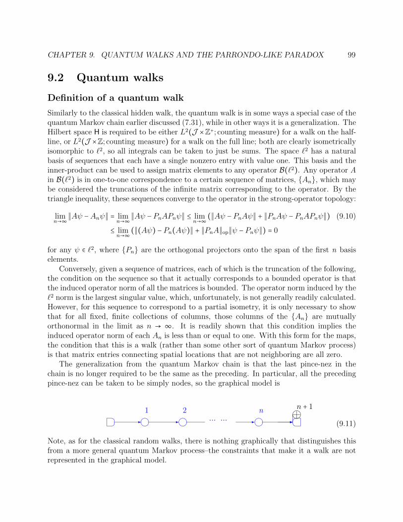
CHAPTER 9. QUANTUM WALKS AND THE PARRONDO-LIKE PARADOX 99
9.2 Quantum walks
Definition of a quantum walk
Similarly to the classical hidden walk, the quantum walk is in some ways a special case of thequantum Markov chain earlier discussed (7.31), while in other ways it is a generalization. TheHilbert space H is required to be either L2(J ×Z+; counting measure) for a walk on the half-line, or L2(J ×Z; counting measure) for a walk on the full line; both are clearly isometricallyisomorphic to `2, so all integrals can be taken to just be sums. The space `2 has a naturalbasis of sequences that each have a single nonzero entry with value one. This basis and theinner-product can be used to assign matrix elements to any operator B(`2). Any operator Ain B(`2) is in one-to-one correspondence to a certain sequence of matrices, An, which maybe considered the truncations of the infinite matrix corresponding to the operator. By thetriangle inequality, these sequences converge to the operator in the strong-operator topology:
limn→∞
∥Aψ −Anψ∥ = limn→∞
∥Aψ − PnAPnψ∥ ≤ limn→∞
(∥Aψ − PnAψ∥ + ∥PnAψ − PnAPnψ∥) (9.10)
≤ limn→∞
(∥(Aψ) − Pn(Aψ)∥ + ∥PnA∥op∥ψ − Pnψ∥) = 0
for any ψ ∈ `2, where Pn are the orthogonal projectors onto the span of the first n basiselements.
Conversely, given a sequence of matrices, each of which is the truncation of the following,the condition on the sequence so that it actually corresponds to a bounded operator is thatthe induced operator norm of all the matrices is bounded. The operator norm induced by the`2 norm is the largest singular value, which, unfortunately, is not generally readily calculated.However, for this sequence to correspond to a partial isometry, it is only necessary to showthat for all fixed, finite collections of columns, those columns of the An are mutuallyorthonormal in the limit as n → ∞. It is readily shown that this condition implies theinduced operator norm of each An is less than or equal to one. With this form for the maps,the condition that this is a walk (rather than some other sort of quantum Markov process)is that matrix entries connecting spatial locations that are not neighboring are all zero.
The generalization from the quantum Markov chain is that the last pince-nez in thechain is no longer required to be the same as the preceding. In particular, all the precedingpince-nez can be taken to be simply nodes, so the graphical model is
k k k - - -⋯ ⋯ - -
1 2 n kn + 1
(9.11)
Note, as for the classical random walks, there is nothing graphically that distinguishes thisfrom a more general quantum Markov process–the constraints that make it a walk are notrepresented in the graphical model.
CHAPTER 9. QUANTUM WALKS AND THE PARRONDO-LIKE PARADOX 100
Orthogonal trigonometric polynomials and measures on S1
Trigonometric orthogonal polynomials3 qj result from the Gram-Schmidt algorithm appliedto 1, z, z−1, z2, z−2, . . . on the unit circle S1 within C with sesquilinear inner-product givenwith respect to some Borel measure µ, ⟨f, g⟩ = ∫S1 fg dµ. To form these, it is useful to startwith the monic orthogonal polynomials on the unit circle, the Szego polynomials, sn. Forany polynomial, define the reciprocal polynomial to be the polynomial with its coefficientsconjugated and flipped in order, so, if p is a nth order polynomial,
preciprocal(z) = znp(1
z) = znp(1
z) (9.12)
where the overline only over the function means to conjugate its coefficients. On S1,
preciprocal(z) = znp (z). In particular, if z is a root of p, then1
zis a root of preciprocal.
Define the Verblunsky coefficients by the values of the Szego polynomials at zero, αn =−sn+1(0). Then, by orthogonality, we have the following Szego recurrence identities for allz ∈ C:
z sn(z) = sn+1(z) + αn sreciprocaln (z) (9.13)
⇔ sreciprocaln+1 (z) = sreciprocal
n (z) − αnz sn(z)and
sn(z) = −αn−1 sreciprocaln (z) + (1 − ∣αn−1∣2) z sn−1(z) (9.14)
⇔ sreciprocaln (z) = −αn−1 sn(z) + (1 − ∣αn−1∣2) sreciprocal
n−1 (z)From the first identity, it follows that
∥sn∥2 = ∫z∈S1
∣sn(z)∣2 dµ(z) = (1 − ∣αn−1∣2)⋯ (1 − ∣α0∣2)µ(S1) (9.15)
By Verblunsky’s theorem, the measure µ, the moments of the measure mj, and theVerblunsky coefficients αj all determine each other. The only condition on the Verblunskycoefficients that they do indeed correspond to some measure is that ∣αj ∣ ≤ 1 for all j.
The monic orthogonal trigonometric polynomials are then given by q0 = 1, and, forj ∈ 1,2, . . .,
qj(z) = z−(j−1)s2j−1(z), q−j(z) = z−jsreciprocal2j (z) (9.16)
3Only a few basic results that are most applicable to quantum walks of this rich topic are presented here.See [87] for details and elaboration.
CHAPTER 9. QUANTUM WALKS AND THE PARRONDO-LIKE PARADOX 101
The orthogonal trigonometric polynomials necessary satisfy a pentadiagonal recurrence re-lation, with first z q0(z) = q1(z) + α0q1(z), then, using (9.13) and (9.14) repeatedly,
zqj(z) = z−jz2s2j−1(z) = z−jz (s2j(z) + α2j−1sreciprocal2j−1 (z)) (9.17)
= z−j (s2j+1(z) + α2jsreciprocal2j (z) + α2j−1z s
reciprocal2j−1 (z))
= z−j (s2j+1(z) + α2jsreciprocal2j (z)
+zα2j−1 (−α2j−2 s2j−1(z) + (1 − ∣α2j−2∣2) sreciprocal2j−2 (z)))
= qj+1(z) + α2jq−j(z) − α2j−1α2j−2qj(z) + α2j−1 (1 − ∣α2j−2∣2) q−(j−1)(z)
and
zq−j(z) = z−jz sreciprocal2j (z) = z−jz (−α2j−1 s2j + (1 − ∣α2j−1∣2) sreciprocal
2j−1 ) (9.18)
= z−j (−α2j−1 (s2j+1 + α2jsreciprocal2j )
+z (1 − ∣α2j−1∣2) (−α2j−2 s2j−1 + (1 − ∣α2j−2∣2) sreciprocal2j−2 ))
= −α2j−1qj+1(z) − α2jα2j−1q−j(z) − α2j−2 (1 − ∣α2j−1∣2) qj+ (1 − ∣α2j−1∣2) (1 − ∣α2j−2∣2) q−(j−1)(z)
Following Cantero, Moral, and Velazquez [6] [7], writing this in matrix form as
[ zq0(z) zq1(z) zq−1(z) ⋯ ] = [ q0(z) q1(z) q−1(z) ⋯ ]Z (9.19)
gives the CMV-matrix Z for the monic orthogonal trigonometric polynomials,
Z =
⎡⎢⎢⎢⎢⎢⎢⎢⎢⎢⎢⎢⎢⎢⎣
α0 α1 (1 − ∣α0∣2) (1 − ∣α1∣2) (1 − ∣α0∣2) 0 ⋯1 −α1α0 − (1 − ∣α1∣2)α0 0 ⋯0 α2 −α1α2 α3 (1 − ∣α2∣2) ⋯0 1 −α1 −α3α2 ⋯0 0 0 α4 ⋯...
......
.... . .
⎤⎥⎥⎥⎥⎥⎥⎥⎥⎥⎥⎥⎥⎥⎦
(9.20)
The matrix Z can be written as the product of two block-diagonal matrices (the columnswithin each 2 × 2-block correspond to the identities in (9.13) and (9.14))
⎡⎢⎢⎢⎢⎢⎢⎢⎢⎢⎢⎢⎣
α0 1 − ∣α0∣21 −α0
α2 1 − ∣α2∣21 −α2
. . .
⎤⎥⎥⎥⎥⎥⎥⎥⎥⎥⎥⎥⎦
⎡⎢⎢⎢⎢⎢⎢⎢⎢⎢⎢⎢⎣
1α1 1 − ∣α1∣21 −α1
α3 ⋯...
. . .
⎤⎥⎥⎥⎥⎥⎥⎥⎥⎥⎥⎥⎦
(9.21)

CHAPTER 9. QUANTUM WALKS AND THE PARRONDO-LIKE PARADOX 102
Using (9.15), the CMV-matrix U for the orthonormal trigonometric polynomials is thengiven by
⎡⎢⎢⎢⎢⎢⎢⎢⎢⎢⎢⎢⎣
α0 ρ0
ρ0 −α0
α2 ρ2
ρ2 −α2
. . .
⎤⎥⎥⎥⎥⎥⎥⎥⎥⎥⎥⎥⎦
⎡⎢⎢⎢⎢⎢⎢⎢⎢⎢⎢⎢⎣
1α1 ρ1
ρ1 −α1
α3 ⋯...
. . .
⎤⎥⎥⎥⎥⎥⎥⎥⎥⎥⎥⎥⎦
(9.22)
for ρj =√
1 − ∣αj ∣2.
Connection to quantum walks–the CMV-matrix
Consider the quantum walk on the half-line Z+∪0 with internal state set J = ↑, ↓, so theHilbert space H is `2(Z×↑, ↓). Then, taking the indices as 0 ↑,0 ↓,1 ↑,1 ↓,2 ↑, . . ., followinga proposal of Grunbaum in [8], the CMV-matrix U above can be used as the map for aquantum walk. With an abuse of notation, for a quantum walk on the line Z with the sameinternal state set and with indices . . . ,−2 ↓,−1 ↑,−1 ↓,0 ↑,0 ↓,1 ↑,1 ↓,2 ↑, . . ., the matrix(underlines indicate indices corresponding spatial location zero) given by the product:
⎡⎢⎢⎢⎢⎢⎢⎢⎢⎢⎢⎢⎢⎢⎢⎢⎢⎢⎢⎢⎣
. . .
α−2 ρ−2
ρ−2 −α−2
α0 ρ0
ρ0 −α0
α2 ρ2
ρ2 −α2
. . .
⎤⎥⎥⎥⎥⎥⎥⎥⎥⎥⎥⎥⎥⎥⎥⎥⎥⎥⎥⎥⎦
(9.23)
⎡⎢⎢⎢⎢⎢⎢⎢⎢⎢⎢⎢⎢⎢⎢⎢⎢⎢⎢⎢⎣
. . ....
⋯ α−3
α−1 ρ−1
ρ−1 −α−1 00 α1 ρ1
ρ1 −α1
α3 ⋯...
. . .
⎤⎥⎥⎥⎥⎥⎥⎥⎥⎥⎥⎥⎥⎥⎥⎥⎥⎥⎥⎥⎦will also be called a CMV-matrix and the αj called the Verblunsky coefficients, althoughthere is no longer a connection to the orthogonal trigonometric polynomials.

CHAPTER 9. QUANTUM WALKS AND THE PARRONDO-LIKE PARADOX 103
Coined quantum walks
Once again, consider the quantum walk on the half-line Z+ ∪ 0 with internal state setJ = ↑, ↓, so the Hilbert space H is `2(Z × ↑, ↓). Then, taking the indices as 0 ↑,0 ↓,1 ↑,1 ↓,2 ↑, . . ., if it is either of the form
⎡⎢⎢⎢⎢⎢⎢⎢⎢⎢⎢⎢⎣
a0 b0
c0 d0
a2 b2
c2 d2
. . .
⎤⎥⎥⎥⎥⎥⎥⎥⎥⎥⎥⎥⎦
⎡⎢⎢⎢⎢⎢⎢⎢⎢⎢⎢⎢⎣
10 11 0
0 ⋯.... . .
⎤⎥⎥⎥⎥⎥⎥⎥⎥⎥⎥⎥⎦
(9.24)
or ⎡⎢⎢⎢⎢⎢⎢⎢⎢⎢⎢⎢⎣
10 11 0
0 ⋯.... . .
⎤⎥⎥⎥⎥⎥⎥⎥⎥⎥⎥⎥⎦
⎡⎢⎢⎢⎢⎢⎢⎢⎢⎢⎢⎢⎣
a0 b0
c0 d0
a2 b2
c2 d2
. . .
⎤⎥⎥⎥⎥⎥⎥⎥⎥⎥⎥⎥⎦
(9.25)
then it is termed a coined walk with coins [ a2j b2j
c2j d2j], which are unitary matrices. The
first form is a CMV-matrix if b2j = c2j is a positive real or zero and if a2j = −d2j; then all theVerblunsky coefficients with odd index are zero and the Verblunsky coefficients with evenindex are given by α2j = −d2j. The second form is the adjoint of a CMV-matrix if the sameconditions hold. The difference between the two forms for a quantum walk is clearly just amatter of transforming the initial state by the unitary matrix
⎡⎢⎢⎢⎢⎢⎢⎢⎢⎢⎢⎢⎣
10 11 0
0 ⋯.... . .
⎤⎥⎥⎥⎥⎥⎥⎥⎥⎥⎥⎥⎦
(9.26)
Therefore, which form is adopted is largely a matter of convention, except for possiblerestrictions on the initial state.
If all the coins are the same, the quantum walk is termed a coined walk with constantcoin. Since the overall phase of the wavefunction is irrelevant, the phase of the determinant
of the coin is arbitrary. Choosing it to be −1, the coin is necessarily of the form [ α β
β −α ]
for some α,β ∈ C with ∣α∣2 + ∣β∣2 = 1. Then the condition for the unitary matrix for thewalk to be a CMV-matrix (or the adjoint of one) is that β is positive real or zero. Similarterminology may be employed for walks on the full line.
CHAPTER 9. QUANTUM WALKS AND THE PARRONDO-LIKE PARADOX 104
9.3 The Parrondo-like paradox for quantum walks
Set-up
Consider the quantum walk on the line Z with internal state set J = ↑, ↓, so the Hilbertspace H is `2(Z × ↑, ↓). Let P+ be the orthogonal projector onto spatial locations withpositive index, P− be the orthogonal projector onto spatial locations with negative index,and P0 be the orthogonal projector onto spatial location zero, so P− +P0 +P+ is the identity.Let U be the unitary operator that gives time evolution for one time step, ρ → UρU∗.Then, after n time steps, an observation is made with an observation set R with σ-algebra∅,A, A,R and base measure τ given by τ(A) = τ(A) = 1. The pince-nez map L is givenby
Lρ = 1Atr ρP+ + 1Atr ρ(P0 + P−) (9.27)
Then, by considering two different initial states, ψψ∗ and ξξ∗, and the geodesic joining them,we can analyze the occurrence and extent of the Parrondo-like paradox.
Showing the paradox is impossible for certain classes of quantumwalks
Let η0↑ be the wavefunction with one for ↑ at location zero and all other amplitudes zeroand η0↓ be the wavefunction with one for ↓ at location zero and all other amplitudes zero.Consider the six following cases for the Verblunsky coefficients determining the CMV-matrixU : (i) αj = ωjα−j for some ω ∈ S1 ⊂ C and all j ∈ Z; (ii) α2j = −ω2jα−2j, α2j+1 = ω2j+1α−2j−1
for some ω ∈ S1 ⊂ C and all j ∈ Z; (iii) αj = α−j for all j ∈ Z; (iv) αj = −α−j for all j ∈ Z; (v)α2j = α−2j, α2j+1 = −α−2j−1 for all j ∈ Z; and (vi) α2j = −α−2j, α2j+1 = α−2j−1 for all j ∈ Z. Withthe preceding set-up, we have the following result:
Theorem 9.3.1 If the Verblunsky coefficients are in any of the preceding six cases, thenfor any initial wavefunctions ψ, ξ in the subspace for spatial location zero, spanCη0↑, η0↓,the Parrondo-like paradox cannot occur.
Proof Let ψ(n) = Unη0↑ and ξ(n) = Unη0↓. Then ξ(n) is related to ψ(n) by the following, foreach n ∈ 1, . . . and j ∈ Z, depending on the case:
i) ξ(n)j,↑ = −ωj−nψ(n)
−j,↓ ξ(n)j,↓ = ω−j−nψ(n)
−j,↑
ii) ξ(n)j,↑ = (−ω)j−nψ(n)
−j,↓ ξ(n)j,↓ = (−ω)−j−nψ(n)
−j,↑
iii) ξ(n)j,↑ = −ψ(n)
−j,↓ ξ(n)j,↓ = ψ(n)
−j,↑
iv) ξ(n)j,↑ = ψ(n)
−j,↓ ξ(n)j,↓ = ψ(n)
−j,↑
v) ξ(n)j,↑ = (−1)j+n+1ψ
(n)−j,↓ ξ
(n)j,↓ = (−1)j+nψ(n)
−j,↑
vi) ξ(n)j,↑ = (−1)j+nψ(n)
−j,↓ ξ(n)j,↓ = (−1)j+nψ(n)
−j,↑
(9.28)
CHAPTER 9. QUANTUM WALKS AND THE PARRONDO-LIKE PARADOX 105
Therefore, in any of the six cases,
tr [ L(Unη0↑η∗0↑U
∗n)∣A L(Unη0↑η∗0↓U∗n)∣A
L(Unη0↓η∗0↑U∗n)∣A L(Unη0↓η∗0↓U
∗n)∣A] = tr [ tr P+ψ(n)ψ(n)∗ tr P+ψ(n)ξ(n)∗
tr P+ξ(n)ψ(n)∗ tr P+ξ(n)ξ(n)∗]
(9.29)
= ⟨(P+ + P−)ψ(n), ψ(n)⟩ ≤ 1
Hence, by theorem 8.4.1, for any initial wavefunctions ψ, ξ in the subspace for spatial loca-tion zero and any point on the geodesic joining [ψ] and [ξ], the paradox cannot occur. ◻
In particular, note this rules out the paradox for the case of constant coin walks of thefirst form with initial wavefunctions ψ, ξ in the subspace for spatial location zero where the
coin is of the form [ α√
1 − ∣α∣2√1 − ∣α∣2 −α ] for some α ∈ C with ∣α∣2 ≤ 1. Using a limit
theorem by Konno [33] [32], we have the following limiting result for more general constantcoin walks (not necessarily in the CMV-matrix form) adopting the second form of coinedquantum walks:
Theorem 9.3.2 If a quantum walk has constant coin presented in the second form, thenfor any initial wavefunctions ψ, ξ in the subspace for spatial location zero, spanCη0↑, η0↓,the Parrondo-like paradox cannot occur in the limit as n→∞.
Proof Adapting the terminology of Konno to our notation, let the coin be given by
[ b ad c
]. The wavefunctions η0↑ and η0↓ are given by β = 1, α = 0 and β = 0, α = 1 re-
spectively. Then, employing Konno’s limit theorem, the limit of the sum of probabilities,
limn→∞
(⟨P+Unτ0↑, Unτ0↑⟩ + ⟨P+Unτ0↓, U
nτ0↓⟩) (9.30)
is given by
∫∣a∣
0
2√
1 − ∣a∣2
π(1 − x2)√
∣a∣2 − x2dx = 1 (9.31)
Hence, by theorem 8.4.1, for any initial wavefunctions ψ, ξ in the subspace for spatial locationzero and any point on the geodesic joining [ψ] and [ξ], the paradox cannot occur in the limitas n→∞. ◻
Examples of quantum walks displaying the paradox to themaximal extent
Example 9.3.3 With the above set-up, take initial wavefunctions ψ = 1√2(η0↑ + η0↓) and
ξ = 1√2(η0↑ − η0↓). Then, halfway on the minimizing geodesic between them, the initial
CHAPTER 9. QUANTUM WALKS AND THE PARRONDO-LIKE PARADOX 106
wavefunction is η0↑. Take all the Verblunsky coefficients to be zero except for α−1, which hasvalue 1√
3. Let U be the corresponding CMV-matrix.
Let ψ(n) = Unψ, ξ(n) = Unξ, and χ(n) = Unη0↑ for n ≥ 1. Then ψ(n) has all amplitudeszero except for 1√
2for ↓ at location n, − 1√
6for ↓ at location n − 1, and 1√
3for ↑ at location
−n; ξ(n) has all amplitudes zero except for − 1√2
for ↓ at location n, − 1√6
for ↓ at location
n − 1, and 1√3
for ↑ at location −n; and χ(n) has all amplitudes zero except for√
23 for ↑ at
location −n and − 1√3
for ↓ at location n − 1. Consequently, PA,n = P ′A,n = 2
3 for all n > 1, yet
P geoA,n = 1
3 for the initial wavefuntion halfway on the minimizing geodesic. By theorem 8.3.2,
this example is on the boundary of allowed values of (PA,n, P ′A,n, P
geoA,n) for the paradox.
Example 9.3.4 Again with the above set-up, let U be the matrix for the constant coin walk
in the second form with coin 1√2[ 1 1−1 1
]. Take ε > 0 small. Take σ1 > 0 sufficiently small
relative to ε such that the normal distribution with mean ε and variance σ21 has neglectfully
small measure for (−∞,0). Take a ∈ (−π2 ,0) and σ2 > 0 such that: (i) the normal distribution
with mean a and variance σ22 has neglectfully small measure outside (−π2 ,0) and (ii) we have
∫k∈(−π
2,0)
− sink√1 + cos2 k
dNormal(a, σ2)(k) =1
3(9.32)
Let ϕ, ζ ∶ Z→ C be given by
ϕj =4
√2σ2
1
πe−σ
21j
2+ı(π2−ε)j = 1√
2π∫
∞
−∞
exp(− (k−(π2−ε))
2
4σ21
+ ıjk)4√
2πσ21
dk (9.33)
≈ 1√2π∫
π
−π
exp(− (k−(π2−ε))
2
4σ21
+ ıjk)4√
2πσ21
dk
ζj =4
√2σ2
2
πe−σ
22j
2+ıaj = 1√2π∫
∞
−∞
exp (− (k−a)2
4σ22
+ ıjk)4√
2πσ22
dk (9.34)
≈ 1√2π∫
π
−π
exp (− (k−a)2
4σ22
+ ıjk)4√
2πσ22
dk

CHAPTER 9. QUANTUM WALKS AND THE PARRONDO-LIKE PARADOX 107
Then, by the inversion of Fourier series,
∑j∈Z
∣ϕj ∣2 = ∫∞
−∞
exp(− (k−(π2−ε))
2
2σ21
)√
2πσ21
dk = 1 (9.35)
∑j∈Z
∣ζj ∣2 = ∫∞
−∞
exp (− (k−a)2
2σ22
)√
2πσ22
dk = 1
∑j∈Zϕjζj = ∫
∞
−∞
exp(− (k−(π2−ε))
2
2σ21
− (k−a)2
4σ22
)4√
2πσ21
4√
2πσ22
dk ≈ 0
Hence, if the initial wavefunctions are taken to be ψ = 12(ζ+ϕ)⊗[ ı
1] and ξ = 1
2(ζ−ϕ)⊗[ ı1
],
they will be properly normalized and approximately orthogonal. Midway on the geodesic
joining them, we have χ = 1√2ζ ⊗ [ ı
1].
Now suppose for the observations we always lump the internal states for any spatial sites,so the σ-algebra for the observations is that generated by only the spatial locations. LetQB be the complete set of mutually commuting, orthogonal projectors for this σ-algebra.Define κ ∶ R→ [−π,π] by
κ(x) =
⎧⎪⎪⎪⎪⎪⎨⎪⎪⎪⎪⎪⎩
arccos x√1−x2
if x ∈ [− 1√2, 1√
2]
0 if x ∈ [ 1√2,∞)
π if x ∈ (−∞,− 1√2]
(9.36)
Then, for each n, let the complete set of commuting projectors R(n)C for the Borel σ-
algebra on [0, π] be given by R(n)C = Q(n⋅κ−1(C))∩Z. By Machida’s limit theorem [37] [38], the
weak*-limit of the measures µ(n) = ⟨R(n)Unψ,Unψ⟩ exists and is given by
µ(∞) ≈1
2Normal(π
2− ε, σ2
2) +1
4(1 − sink√
1 + cos2 k)Normal(−a, σ2) (9.37)
+ 1
4(1 + sink√
1 + cos2 k)Normal(π + a, σ2)
Similarly, the weak*-limit of the measures ν(n) = ⟨Q(n)Unξ,Unξ⟩ exists and is given by thesame expression. For both of these, there is approximately 1
2 + 14(1 − 1
3) = 2
3 probability to
have k ∈ [0, π2 ), which corresponds to spatial locations with positive index j. The weak*-limitof the measures τ (n) = ⟨Q(n)Unχ,Unχ⟩ also exists and is given by
τ (∞) ≈ 1
2(1 − sink√
1 + cos2 k)Normal(−a, σ2) +
1
2(1 + sink√
1 + cos2 k)Normal(π + a, σ2) (9.38)

CHAPTER 9. QUANTUM WALKS AND THE PARRONDO-LIKE PARADOX 108
However, now there is only approximately 12(1 − 1
3) = 1
3 probability to have k ∈ [0, π2 ). Thesevalues of two-thirds for PA, two-thirds for P ′
A, and one-third for P geoA can be arbitrarily
closely approached by taking ε, σ1, and σ2 sufficiently small. By theorem 8.3.2, this examplecan approach arbitrarily closely to the boundary of allowed values of (PA, P ′
A, PgeoA ) for the
paradox.
Remark The results of the preceding example also hold for the commonly employed
Hadamard coin 1√2[ 1 1
1 −1]. Then the matrix U is the adjoint of a CMV-matrix with
all Verblunsky coefficients with even index equal to 1√2. For the Hadamard coin, we take
initial wavefunctions to be ψ = 12(ζ + ϕ) ⊗ [ ı
−1] and ξ = 1
2(ζ − ϕ) ⊗ [ ı−1
], so we have
χ = 1√2ζ ⊗ [ ı
−1], where
ϕj =4
√2σ2
1
πe−σ
21j
2+ıεj (9.39)
ζj =4
√2σ2
2
πe−σ
22j
2−ı(π2+a)j (9.40)
for a, ε, σ1, and σ2 as in the given example. The coin utilized in the example was chosen toagree with that used by Machida [37] [38].

109
Bibliography
[1] M. Abramowitz and I.A. Stegun, eds. Handbook of Mathematical Functions. NationalBureau of Standards, Applied Mathematics Series 55. Washington: U.S. GovernmentPrinting Office, 1964, pp. 773–774.
[2] Y. Aharonov, S. Popescu, and J. Tollaksen. “A time-symmetric formulation of quantummechanics”. In: Physics Today (2010).
[3] E. Beckenstein and L. Narici. Topological Vector Spaces. Monographs and Textbooksin Pure and Applied Mathematics 95. New York: Marcel Dekker, Inc., 1985, pp. 87–88.
[4] J.S. Bell. “On the Einstein-Podolsky-Rosen Paradox”. In: Physics 1 (1964).
[5] B.H. Bennet et al. “Teleporting an unknown quantum state via dual classical andEinstein-Podolsky-Rosen channels”. In: Physical Review Letters 70.13 (1993).
[6] M.J. Cantero, L. Moral, and L. Velazquez. “Five-dimensional matrices and zeros oforthogonal polynomials on the unit circle”. In: Linear Algebra Applications 362 (2003),pp. 29–56.
[7] M.J. Cantero, L. Moral, and L. Velazquez. “Minimal representations of unitary oper-ators and orthogonal polynomials on the unit circle”. In: Linear Algebra Applications408 (2005), pp. 40–65.
[8] M.J. Cantero et al. “Matrix valued Szego polynomials and quantum random walks”.In: Communications on Pure and Applied Mathematics 63 (2010), pp. 464–507.
[9] A. Cho. “Furtive approach rolls back the limits of quantum uncertainty”. In: Science(2011), pp. 690–693.
[10] B. Cirel’son. “Quantum Generalizations of Bell’s Inequality”. In: Letters un Mathe-matical Physics 4 (1980).
[11] J.F. Clauser et al. “Proposed experiment to test local hidden-variable theories”. In:Physical Review Letters 23 (1969).
[12] J.W. Demmel. Applied Numerical Linear Algebra. Society for Industrial and AppliedMathematics 199-200. Philadelphia: American Mathematical Society, 1997.
[13] J. Diestel, J.H. Fourie, and J. Swart. The Metric Theory of Tensor Products: Grothendieck’sResume Revisited. Providence: American Mathematical Society, 2008, p. 7.

BIBLIOGRAPHY 110
[14] J. Diestel and J.J. Uhl. Vector Measures. Mathematical surveys 15. Providence: Amer-ican Mathematical Society, 1977, pp. 217–219.
[15] P.A.M. Dirac. The Principles of Quantum Mechanics. Oxford: Claredon Press, 1930,p. 35.
[16] P.A.M. Dirac. The Principles of Quantum Mechanics. Oxford: Claredon Press, 1930,p. 36.
[17] H.R. Dowson. Spectral Theory of Linear Operators. London Mathematics Society Mono-grams 12. London: Academic Press, Inc., 1978, pp. 50–52.
[18] R. Durrett. Probability Theory and Examples. 3rd ed. Belmont: Brooks/Cole, 2005,p. 108.
[19] E.G. Effros and Z.J. Ruan. Operator Spaces. London Mathematical Society Monographs–New Series 23. Oxford: Clarendon Press, 2000, p. 25.
[20] W. Feller. An Introduction to Probability Theory and its Applications. New York: JohnWiley & Sons, Inc., 1950, pp. 430–432.
[21] F.Hausdorff. Set Theory. 2nd ed. New York: Chelsea Publishing Company, 1962, pp. 96–108.
[22] F.Hausdorff. Set Theory. 2nd ed. New York: Chelsea Publishing Company, 1962, p. 72.
[23] A.P. Flitney, J. Ng, and D. Abbott. “Quantum Parrondo’s Games”. In: Physica A 314(2002), pp. 35–42.
[24] A.M. Gleason. “Measures on the closed subspaces of a Hilbert space”. In: Journal ofMathematics and Mechanics 6.6 (1957), pp. 885–893.
[25] F.A. Grunbaum. “An urn model associated with Jacobi polynomials”. In: Communi-cations in Applied Mathematics and Computational Science 5.1 (2010), pp. 55–63.
[26] F.A. Grunbaum and M. Pejic. “Maximal Parrondo’s Paradox for Classical and Quan-tum Markov Chains”. In: Communications in Mathematical Physics (2015). submitted.
[27] Jasper Hopkins. Nicholas of Cusa On Learned Ignorance: A Translation and Appraisalof De Docta Ignorantia. Minneapolis: The Arthur J. Banning Press, 1981, p. 51.
[28] F.V. Jensen. Bayesian Networks and Decision Graphs. Statistics for Engineering andInformation Science. New York: Springer-Verlang, 2001, pp. 35–44.
[29] F.V. Jensen. Bayesian Networks and Decision Graphs. Statistics for Engineering andInformation Science. New York: Springer-Verlang, 2001, pp. 37,65.
[30] S. Kochen and E.P. Specker. “The Problem of Hidden Variables in Quantum Mechan-ics”. In: Journal of Mathematics and Mechanics 17.1 (1967), pp. 75–81.
[31] S. Kochen and E.P. Specker. “The Problem of Hidden Variables in Quantum Mechan-ics”. In: Journal of Mathematics and Mechanics 17.1 (1967).

BIBLIOGRAPHY 111
[32] N. Konno. “A new type of limit theorem for the one-dimensional quantum randomwalk”. In: Journal of the Mathematical Society of Japan 57 (2005), pp. 1179–1195.
[33] N. Konno. “Limit theorems and absorption problems for quantum random walks inone dimension”. In: Quantum Information and Computation 2 (2002). Special issue,pp. 578–595.
[34] K. Kuratowski. Topology. Vol. 1.
[35] K. Kuratowski. Topology. Vol. 1.
[36] A.D. Lorenzo. “Reassessment of Leggett Inequality”. In: Foundations of Physics 43(2011), pp. 685–698.
[37] T. Machida. “A quantum walk with a delocalized initial state: contribution from acoin-flip operator”. In: International Journal of Quantum Information ().
[38] T. Machida. “Realization of the probability laws in the quantum central limit theoremsby a quantum walk”. In: Quantum Information and Computation 13 (2013), pp. 430–438.
[39] J.J. Martin. Bayesian Decision Problem and Markov Chains. New York: John Wiley& Sons, Inc., 1967, p. 62.
[40] N.D. Mermin. Quantum Computer Science. Cambridge: Cambridge University Press,2007, pp. 21–23.
[41] D.A. Meyer. “Noisy quantum Parrondo game”.
[42] J.R. Munkres. Topology. 2nd ed. Upper Saddle River: Prentice Hall, 2000, p. 167.
[43] J.R. Munkres. Topology. 2nd ed. Upper Saddle River: Prentice Hall, 2000, pp. 182–185.
[44] J.R. Munkres. Topology. 2nd ed. Upper Saddle River: Prentice Hall, 2000, pp. 62–74.
[45] J.R. Munkres. Topology. 2nd ed. Upper Saddle River: Prentice Hall, 2000, p. 225.
[46] J.R. Norris. Markov Chains. Cambridge Series in Statistical and Probabilistic Mathe-matics. Cambridge: Cambridge University Press, 1997, pp. 40–46.
[47] N.R. Norris. Markov Chains. Cambridge Series in Statistical and Probabilistic Math-ematics. Cambridge: Cambridge University Press, 1997, pp. 33–39.
[48] J.C. Oxtoby. “Invariant measures in groups which are not locally compact”. In: Trans-actions of the American Mathematical Society 60.2 (1946), pp. 215–237.
[49] J. Parrondo and P. Espagnol. “Criticism of Feynman’ analysis of the ratchet as anengine”. In: American Journal of Physics 64 (1996).
[50] G.K. Pedersen. C*-algebras and their Automorphism Groups. London: Academic Press,Inc., 1979, p. 52.
[51] A.L. Peressini. Ordered Topological Vector Spaces. Harper’s Series in Modern Mathe-matics. New York: Harper & Row, 1967, p. 7.
BIBLIOGRAPHY 112
[52] M.M. Rao. Measure Theory and Integration. New York: John Wiley & Sons, Inc., 1987,pp. 339–344.
[53] H.L. Royden. Real Analysis. 3rd ed. Upper Saddle River: Prentice Hall, 1988, pp. 276–278.
[54] H.L. Royden. Real Analysis. 3rd ed. Upper Saddle River: Prentice Hall, 1988, pp. 307–309.
[55] H.L. Royden. Real Analysis. 3rd ed. Upper Saddle River: Prentice Hall, 1988, p. 278.
[56] H.L. Royden. Real Analysis. 3rd ed. Upper Saddle River: Prentice Hall, 1988, pp. 268–270.
[57] H.L. Royden. Real Analysis. 3rd ed. Upper Saddle River: Prentice Hall, 1988, p. 357.
[58] H.L. Royden. Real Analysis. 3rd ed. Upper Saddle River: Prentice Hall, 1988, pp. 331–335.
[59] H.L. Royden. Real Analysis. 3rd ed. Upper Saddle River: Prentice Hall, 1988, pp. 197–198.
[60] H.L. Royden. Real Analysis. 3rd ed. Upper Saddle River: Prentice Hall, 1988, p. 201.
[61] H.L. Royden. Real Analysis. 3rd ed. Upper Saddle River: Prentice Hall, 1988, p. 274.
[62] H.L. Royden. Real Analysis. 3rd ed. Upper Saddle River: Prentice Hall, 1988, p. 284.
[63] H.L. Royden. Real Analysis. 3rd ed. Upper Saddle River: Prentice Hall, 1988, pp. 248–249.
[64] H.L. Royden. Real Analysis. 3rd ed. Upper Saddle River: Prentice Hall, 1988, pp. 237–238.
[65] H.L. Royden. Real Analysis. 3rd ed. Upper Saddle River: Prentice Hall, 1988, p. 240.
[66] H.L. Royden. Real Analysis. 3rd ed. Upper Saddle River: Prentice Hall, 1988, p. 223.
[67] H.L. Royden. Real Analysis. 3rd ed. Upper Saddle River: Prentice Hall, 1988, p. 25.
[68] H.L. Royden. Real Analysis. 3rd ed. Upper Saddle River: Prentice Hall, 1988, p. 267.
[69] H.L. Royden. Real Analysis. 3rd ed. Upper Saddle River: Prentice Hall, 1988, p. 259.
[70] H.L. Royden. Real Analysis. 3rd ed. Upper Saddle River: Prentice Hall, 1988, p. 53.
[71] H.L. Royden. Real Analysis. 3rd ed. Upper Saddle River: Prentice Hall, 1988, p. 274.
[72] H.L. Royden. Real Analysis. 3rd ed. Upper Saddle River: Prentice Hall, 1988, pp. 303–304.
[73] H.L. Royden. Real Analysis. 3rd ed. Upper Saddle River: Prentice Hall, 1988, p. 200.
[74] H.L. Royden. Real Analysis. 3rd ed. Upper Saddle River: Prentice Hall, 1988, p. 309.
[75] H.L. Royden. Real Analysis. 3rd ed. Upper Saddle River: Prentice Hall, 1988, p. 179.
[76] H.L. Royden. Real Analysis. 3rd ed. Upper Saddle River: Prentice Hall, 1988, p. 53.

BIBLIOGRAPHY 113
[77] R.A. Ryan. Introduction to Tensor Products of Banach Spaces. Springer Monographsin Mathematics. London: Springer-Verlag, 2002.
[78] R.A. Ryan. Introduction to Tensor Products of Banach Spaces. Springer Monographsin Mathematics. London: Springer-Verlag, 2002, p. 94.
[79] Shoichiro Sakai. Markov Chains. Ergebnisse der Mathematik und ihrer Grenzgebiete60. New York: Springer-Verlang, 1971, pp. 102–103.
[80] Shoichiro Sakai. Markov Chains. Ergebnisse der Mathematik und ihrer Grenzgebiete60. New York: Springer-Verlang, 1971, p. 48.
[81] Z. Semadeni. Banach Spaces of Continuous Functions. Vol. 1.
[82] Z. Semadeni. Banach Spaces of Continuous Functions. Vol. 1.
[83] Z. Semadeni. Banach Spaces of Continuous Functions. Vol. 1.
[84] E. Seneta. Non-negative Matrices and Markov Chains. Springer series in Statistics.New York: Springer-Verlang, 2002, pp. 35–44.
[85] C.E. Shannon and W. Weaver. The Mathematical Theory of Communication. Urbana:University of Illinois Press, 1949.
[86] W. Sierpinnski. Cardinal and Ordinal Numbers. Monografie Matematyczne 34. Warsaw:Panstwowe Wydawnictwo Naukowe.
[87] B. Simon. Orthogonal Polynomials on the Unit Circle. Vol. 2. American Mathemati-cal Society Colloquium Publications 54. Providence: American Mathematical Society,2005.
[88] W.F. Stinespring. “Positive functions on C *-algebras”. In: Proceedings of the AmericanMathematical Society 6.2 (1955), pp. 211–216.
[89] G. Szego. Orthogonal Polynomials. American Mathematical Society Colloquium Pub-lications 23. New York: American Mathematical Society, 1939.
[90] A. Wilansky. Modern Methods in Topological Vector Spaces. New York: McGraw-Hill,Inc., 1978, p. 237.
[91] A. Wilansky. Modern Methods in Topological Vector Spaces. New York: McGraw-Hill,Inc., 1978, p. 17.
[92] W.K. Wooters and W.H. Zureck. “A single quantum cannot be cloned”. In: Nature299 (1982), pp. 802–803.
114
Appendix A
General propositions
A.1 Banach space propositions
Notation Let A, B,. . . denote Banach spaces.
Proposition A1.1 Maps in B(A,B) are continuous in the weak topologies on A and B.
Proof Take any such map L. For any weak neighborhood
N (La;φ1, . . . , φn; ε) = b ∈ B∣ ∣φj(b −La)∣ < ε for j ∈ 1, . . . , n (A.1)
with a ∈ A, φ1, . . . , φn ∈ B∗, and ε > 0 we have
L (N (a;L∗φ1, . . . , L∗φn; ε)) = N (La;φ1, . . . , φn; ε) ◻ (A.2)
Corollary A1.2 A map in L ∈ B(A,B) is uniquely determined by its values on a weaklydense subset.
Comment Starting with a weakly dense subset that is a vector space, its norm closureis necessarily a linear subspace by the properties of Cauchy sequences. Since this subspaceis convex, by the separating theorem [65], it cannot be weakly dense unless it is the entirespace; hence, a weakly dense subset is necessarily also norm-dense. This argument is notentirely satisfactory since the separating theorem uses the Hahn-Banach theorem [66], whichdepends on the axiom of choice [67]. This deficiency will be rectified for the situation ofinterest by proposition B1.3 below.
The following important proposition is assigned as an exercise in [91].
Proposition A1.3 Let A and B be Banach spaces. A subset V of A that is a vector spaceuniquely determines a map L ∈ B(A,B) if V is dense in the norm topology on A and theoperator norm of L restricted to V is bounded. The operator norm of L shares the bound tothe operator norm of its restriction.

APPENDIX A. GENERAL PROPOSITIONS 115
Proof Since a continuous function is uniquely determined by its values on a weakly densesubset, and since the norm topology is finer than the weak topology, if L exists, it is uniqueby A1.2. For any a ∈ A, define La as the limit of the Cauchy sequence ⟨Laj⟩∞j=1, where
⟨aj⟩∞j=1 is any Cauchy sequence converging to a composed of elements of V. The choice of
Cauchy sequence does not matter because, given another Cauchy sequence ⟨bj⟩∞j=1 converging
to a composed of elements of V, then ⟨aj − bj⟩∞j=1 is a Cauchy sequence converging to zero,
so ⟨L(aj − bj)⟩∞j=1 is a Cauchy sequence converging to zero. Since the product of a Cauchysequence with a scalar is a Cauchy sequence and the sum of two Cauchy sequences is aCauchy sequence, L is linear. ◻
A.2 Hilbert space propositions
Notation Let H be a Hilbert space.
Proposition A2.1 Convergence of a countable sum of disjoint (PjPk = 0 if j ≠ k), or-thogonal projectors, ∑j Pj, to an orthogonal projector P is equivalent in the following fourtopologies on B(H): ultrastrong-operator, strong-operator, ultraweak-operator1, and weak-operator.
Proof The weak-operator topology is courser than the other three, so convergence in anyof the others implies convergence in it. Suppose convergence occurs in the weak-operatortopology, so for any ψ,ψ′ ∈ H,
limk→∞
⟨(P −k
∑j=1
Pj)ψ,ψ′⟩ = 0 (A.3)
Then, for any fixed k,
⟨Pk
∑j=1
Pjψ,ψ′⟩ = lim
m→∞⟨m
∑l=1
Pjk
∑j=1
Pjψ,ψ′⟩ = ⟨
k
∑j=1
Pjψ,ψ′⟩ (A.4)
Since ψ,ψ′ were arbitrary, P ∑kj=1Pj = ∑k
j=1Pj. Similarly, (∑kj=1Pj)P = ∑k
j=1Pj. Therefore,
(P −∑kj=1Pj)
2 = P − ∑kj=1Pj, so P − ∑k
j=1Pj is itself an orthogonal projector (it is clearlyself-adjoint). Then, by taking ψ = ψ′, this implies
limk→∞
∥(P −k
∑j=1
Pj)ψ∥ = 0 (A.5)
so convergence necessarily also occurs in the strong-operator topology. Since the sequenceof operators ⟨P −∑k
j=1Pj⟩∞
k=1is bounded in operator norm (all being projectors), the con-
vergence necessarily occurs in the ultrastrong-operator topology as well. However, the1Same as the weak* topology.
APPENDIX A. GENERAL PROPOSITIONS 116
ultrastrong-operator topology is finer than the others, so convergence in it implies con-vergence in the other three. ◻
A.3 Transition function propositions
Notation For the following, sets will be denoted X , Y,. . . and σ-algebras by E , F ,. . .. Thespaces of finite, signed-measures on the given set with the given σ-algebra will be denotedM(X ;E), M(Y;F),. . .. These are Banach spaces using the total variation norm. Note–byconvention product measures are written using × although they are actually tensor productsand should be written using ⊗ (see [81] for a use of the latter notation).
Following [52], we have the following:
Definition A3.1 For σ-algebras E on X and F on Y, a function τ(⋅∣⋅) ∶ F × X → R is atransition function if: (i) for each x ∈ X , τ(⋅∣x) ∈M(Y ;F); and (ii) for each B ∈ F , τ(B∣⋅)is a bounded, E-measurable function on X .
If τ(⋅∣⋅) is positive and has the additional property that τ(Y ∣⋅) = 1X , then it is termed atransition probability function. The transition functions for specified (E , X , F , Y) clearlyform a vector space. They form a Banach space using the norm
∥τ(⋅∣⋅)∥ = supx∈X
∥τ(⋅∣x)∥total variation (A.6)
A transition function τ(⋅∣⋅) with specified data (E , X , F , Y) induces a linear map L ∈B(M(X ;E),M(Y;F)) via
(Lµ)(B) = ∫x∈X
τ(B∣x)dµ(x) (A.7)
Not every bounded linear map is induced by a transition function; in general, a pseudo-transition function is required (see B2.7 and B2.8). However, we do have the following:
Proposition A3.2 If L ∈ B(M(X ;E),M(Y;F)) and K ∈ B(M(Y;F),M(Z;G)) are bothinduced by transition functions, then the composition K L is also induced by a transitionfunction.
Proof Let L and K be such maps, with associated transition functions τ(⋅∣⋅) and ν(⋅∣⋅).Define ω(⋅∣⋅) by
ω(C ∣x) = ∫y∈Y
ν(C ∣y)d(τ(⋅∣x))(y) (A.8)
for C ∈ G and x ∈ X . Then ω(⋅∣x) ∈ M(Z;G). To see that ω(C ∣⋅) is E-measurable, notethat, since ν(C ∣⋅) is F -measurable and bounded, there is a sequence of simple functions
APPENDIX A. GENERAL PROPOSITIONS 117
⟨∑k bjk1Bjk⟩ converging uniformly to it. By the dominated convergence theorem [68], wethen have
ω(C ∣x) = limj→∞
∑k
bjkτ(Bjk∣x) (A.9)
By [69], finite sums of measurable functions are measurable and the pointwise limit of asequence of measurable functions is measurable, so ω(C ∣⋅) is measurable. Hence, ω(⋅∣⋅) is atransition function.
Now take any µ ∈M(X ;E) and C ∈ G. Then, using the preceding results,
((K L)(µ))(C) = ∫y∈Y
ν(C ∣y)d(Lµ)(y) = limj→∞
∑k
bjk(Lµ)(Bjk) (A.10)
= limj→∞
∑k
bjk ∫x∈X
τ(Bjk∣x)dµ(x) = ∫x∈X
ω(C ∣x)dµ(x)
Hence, K L is induced by the transition function ω(⋅∣⋅). ◻
Proposition A3.3 If L ∈ B(M(X ;E),M(Z;G)) andK ∈ B(M(Y;F),M(W;H)) are bothinduced by transition functions, then the tensor product map K ⊗L is well-defined and alsoinduced by a transition function.
Proof Let L and K be such maps, with associated transition functions τ(⋅∣⋅) and ν(⋅∣⋅).Define ω(⋅∣⋅) by ω(⋅∣x, y) = τ(⋅∣x) × ν(⋅∣y) for each x ∈ X and y ∈ Y. Then ω(⋅∣x, y) is clearlyin M(X × Y;I), where I is the σ-algebra generated by the rectangular subsets R = E × F .The rectangular subsets form a semialgebra2 Then the finite union of rectangular sets is analgebra.
Following Hausdorff [21], let R0 be the rectangular subsets R. For each ordinal α, letRα be the collection of subsets of X × Y that are the countable intersection of subsets fromthe various collections Rβ for ordinals β < α if α is even and that are the countable union ofsubsets from the various collections Gβ for ordinals β < α if α is odd (where all limit ordinals–those without a predecessor–taken even). For clarification, using the standard notation [70],R1 =Rσ, R2 =Rσδ, and so on for the finite ordinals.
Fix any ordinal α and suppose that for all subsets B in all collections Rβ for β < α wehave the following property: there is an I-measurable ω(B∣⋅) such that
((L⊗K)µ)(B) = ∫(x,y)∈X×Y
ω(B∣x, y)dµ(x, y) (A.11)
for any I-measure µ on X × Y. Take any C ∈ Rα. If α is odd, we have a sequence ⟨Bj⟩ ofsubsets from the various Rβ with β < α such that C = ⋃j Bj. Let ω(C ∣⋅) = ⋁j ω(Bj ∣⋅). Thenω(C ∣⋅) is I-measurable (see [69]) and we can extend L⊗K by
((L⊗K)µ)(C) = ∫(x,y)∈X×Y
ω(C ∣x, y)dµ(x, y) (A.12)
2A collection of sets is a semialgebra if it is closed under intersection and the complement of any set isa finite union of sets in the collection.

APPENDIX A. GENERAL PROPOSITIONS 118
for any I-measure µ on X ×Y; hence, since C was arbitrary, Rα has the property. Similarly,if α is even, we have a sequence ⟨Bj⟩ of subsets from the various Rβ with β < α such thatC = ⋂j Bj. Let ω(C ∣⋅) = ⋀j ω(Bj ∣⋅). Then ω(C ∣⋅) is measurable and we can extend L⊗K by(A.12); hence, Rα also has the property.
However, R0 has the property–for any I-measure µ, (L⊗K)µ is uniquely determined onthe rectangular subsets by
((L⊗K)µ)(A ×B) = ∫(x,y)∈X×Y
τ(A∣x)ν(B∣y)dµ(x, y) (A.13)
and ω(A×B∣x, y) = τ(A∣x)ν(B∣y) is I-measurable (see [69])–so by transfinite induction [22] [86]all the Rα have the property. Following Kuratowski [34], the σ-algebra I is given by theunion ⋃αRα. Therefore, ω(⋅∣⋅) is a transition function and induces a well-defined tensorproduct map K ⊗L. ◻
Comment The preceding proof does not depend on the axiom of choice since the uniononly needs to be taken up to the ordinal number for the minimal uncountable well-orderedset [21] [34], whose existence does not depend on the axiom of choice [44].

119
Appendix B
Propositions for option I
B.1 Measures
Notation For the following, sets will be denoted X , Y,. . . and σ-algebras by E , F ,. . .. Thespaces of finite, signed-measures on the given set with the given σ-algebra will be denotedM(X ;E), M(Y;F),. . .. These are Banach spaces using the total variation norm.
Definition B1.1 A subset of signed-measures, M ⊂ M(X ;E), is absolutely-continuous-complete if, for any µ in M, all signed-measures absolutely continuous with respect to ∣µ∣ arealso in M.
Proposition B1.2 Any absolutely-continuous-complete subset that is a vector space isdirected-complete1.
Proof Let M ⊂ M(X ;E) be such a subset. Given any upward-directed subset B ⊂ M ,bounded by above by some ρ ∈M , define ⋁µ∈B µ by, for any E ∈ E ,
(⋁µ∈B
µ)(E) = supµ∈B
µ(E) (B.1)
This exists since it is bounded from above by ρ(E). It is readily seen that ⋁µ∈B µ is greaterthan or equal to (using the partial ordering) any µ ∈ B and that, given any other ν ∈ Mwith that property, ⋁µ∈B µ ≤ ν. Given any countable collection of disjoint, measurable sets,E∞j=1 ⊂ E , by the upward-directed property and the countable additivity of each µ ∈ B,
n
∑j=1
(⋁µ∈B
µ)(Ej) + (⋁µ∈B
µ)(∞
⋃j=n+1
Ej) ≤ (⋁µ∈B
µ)(∞
⋃j=1
Ej) ≤∞
∑j=1
(⋁µ∈B
µ)(Ej) (B.2)
1A partially-ordered subset is upward-directed if, given any two elements, there is a third that is greaterthan or equal to both. A set is directed-complete if any bounded, upward-directed subset has a supremum.

APPENDIX B. PROPOSITIONS FOR OPTION I 120
for any n ∈ 1,2, . . .. Since ν ≤ ⋁µ∈B µ ≤ ρ for any ν ∈ B, and both ρ and ν are countablyadditive, both (⋁µ∈B µ) (⋃∞
j=n+1Ej)→ 0 and the tail sum ∑∞j=n+1 (⋁µ∈B µ) (Ej)→ 0 as n→∞,
so∞
∑j=1
(⋁µ∈B
µ)(Ej) ≤ (⋁µ∈B
µ)(∞
⋃j=1
Ej) ≤∞
∑j=1
(⋁µ∈B
µ)(Ej) (B.3)
Therefore, ⋁µ∈B µ is countably additive, so it is a signed E-measure. Its total variationnorm is bounded by the total variation norm of ρ ∨ (−ν) for any particular ν ∈ B. Sinceν ≤ ⋁µ∈B µ ≤ ρ, ⋁µ∈B µ is absolutely continuous with respect to ∣ρ∣ + ∣ν∣, so ⋁µ∈B µ ∈M . ◻
Comment The following proposition corrects the defect mentioned after A1.2 for theparticular case required.
For the following two propositions, let G be the σ-algebra generated by the rectangularsubsets E ×F . Let the absolutely-continuous-complete subsets M ⊂M(X ;E), N ⊂M(Y;F),and Q ⊂M(X × Y;G) also be vector spaces.
Proposition B1.3 If M ⊗N is weakly dense in Q, then it is norm-dense in Q.
Proof Suppose there were some measure µ ∈ C+ not in the norm-closure of M⊗N , so thereis some ε > 0 such that ∥µ− ν∥total variation > ε for all ν ∈M ⊗N . By Hahn-decomposition [71]and the absolutely-continuous-completeness property of M and N, if ν ∈ M ⊗ N , then∣ν∣ ∈ M ⊗ N . Let µ ⊥ ∣ν∣ be the singular part of µ with respect to ∣ν∣ using Lebesguedecomposition [55]. The set of G-measures µ ⊥ ∣ν∣∣ν ∈M ⊗N is lower-bound by the zero-measure. It is downward-directed since µ ⊥ (∣ν∣ + ∣ν′∣) is less than or equal to (in the partialordering) both µ ⊥ ∣ν∣ and µ ⊥ ∣ν′∣ for any ν, ν′ ∈M⊗N . Hence, by the preceding proposition,the G-measure τ = ⋀ν∈M⊗N µ ⊥ ∣ν∣ exists. Furthermore, from its definition in the precedingproof, this measure has total-variation norm greater than or equal to ε. Let ρ∥τ be the ab-solutely continuous part of ρ with respect to τ using Lebesgue decomposition. Now considerthe bounded, linear functional Φ ∈M(X × Y ;G)∗ given by Φρ = (ρ∥τ)(X × Y). This is zeroon M ⊗N , yet Φµ = ∥τ∥total variation ≥ ε; hence, µ is not in the weak-closure of M ⊗N . ◻
Proposition B1.4 If M ⊗N is norm-dense in Q, then M+ ⊗R+ N+ is norm-dense in Q+.
Proof By Hahn-decomposition and the absolutely-continuous-completeness property of Mand N, the measures in M ⊗N are total-variation norm-dense for the measures Q+. Givenany measure µ = ∑j νj ⊗ τj ∈ M ⊗N , it is absolutely continuous with respect to the prod-
uct measure ρ = (∑j ∣νj ∣) ⊗ (∑k ∣τk∣), which is in M ⊗ N by Hahn-decomposition and theabsolutely-continuous-completeness property of M and N. By the Radon-Nikodym theo-rem [53], there is a positive function dµ
dρ ∈ L1(X × Y;ρ) such that µ = dµdρρ. By proposition
B3.1 below, dµdρ can be arbitrarily well approximated in total-variation norm by elements of
L1 (X ;∑j ∣νj ∣)+ ⊗R+ L1 (Y;∑k ∣τk∣)+. ◻
APPENDIX B. PROPOSITIONS FOR OPTION I 121
Proposition B1.5 The total-variation norm is a cross-norm for product measures.
Proof Let µ ∈M(X ;E) and ν ∈M(Y;F). By Hahn decomposition, ∣µ × ν∣ = ∣µ∣ × ∣ν∣, so
∥µ × ν∥ = ∣µ × ν∣(X × Y) = ∣µ∣(X )∣ν∣(Y) = ∥µ∥∥ν∥ ◻ (B.4)
Proposition B1.6 If µ is a σ-finite measure on X , then there is no uncountable collectionAα of subsets of X with the properties that µ(Aα) > 0 for all α and µ(Aα ∩Aβ) = 0 for allα ≠ β.
Proof Suppose otherwise. Since µ is σ-finite, there is a countable, disjoint collection Bjof subsets of X such that each Bj has finite µ-measure and their union ∪jBj is the entirespace X . Now suppose there is some ε > 0 and j such that for infinitely many of the Aα,µ(Bj ∩ Aα) > ε. That immediately contradicts µ(Bj) being finite. Therefore, it must bethe case that for any ε > 0 and j, only finitely many of the Aα satisfy µ(Bj ∩ Aα) > ε.Let Ak be the countable collection formed by taking the union over all j and over allε ∈ 1,2−1,2−2, . . . of such Aα. However, this also leads to a contradiction, since for anyAβ ∉ Ak, µ(Aβ ∩Bj) = 0 for all j, yet 0 < µ(Aβ) = ∑j µ(Aβ ∩Bj) = 0. ◻
B.2 Maps on subspaces of the space of measures
Let M ⊂M(X ;E) be any absolutely-continuous-complete, norm-closed subspace.
Proposition B2.1 Any positive linear map L ∈ B(M,M(Y;F)) has
∥L∥op = supµ∈M+,µ(X )≤1
Lµ(Y) (B.5)
Proof Since L is positive, ∣Lµ∣ = ∣L(µ+−µ−)∣ = ∣L(µ+)−L(µ−)∣ ≤ L(µ+)+L(µ−) = L∣µ∣ usingHahn decomposition, so
supµ∈M+,µ(X )≤1
Lµ(Y) ≤ ∥L∥op = sup∣µ∣(X )≤1
∣Lµ∣(Y) ≤ supµ∈M+,µ(X )≤1
Lµ(Y) ◻ (B.6)
Proposition B2.2 The space of maps B(M,M(Y ;F)) is a vector lattice2.
2A partially-ordered, vector space A is a vector lattice if for any a,b ∈ A, there are elements a ∨ b anda ∧ b such that a ∨ b is greater than or equal to both a and b, but is less than or equal to any other elementwith that property and a ∧ b is less than or equal to both a and b, but is greater than or equal to any otherelement with that property.
APPENDIX B. PROPOSITIONS FOR OPTION I 122
Proof For any maps K,L ∈ B(M,M(Y ;F)) define K ∨ L by (K ∨ L)(µ)(F ) for µ ∈ M+
and F ∈ F being
sup
⎧⎪⎪⎪⎪⎪⎨⎪⎪⎪⎪⎪⎩
n
∑j=1
m
∑k=1
max(Kµj)(Fk), (Lµj)(Fk)
RRRRRRRRRRRRRRRRRR
n,m ∈ 1,2, . . .µ1, . . . , µn ∈M+
disjoint F1, . . . , Fm ∈ F∑nj=1 µj = µ,⋃mj=1Fj = F
⎫⎪⎪⎪⎪⎪⎬⎪⎪⎪⎪⎪⎭
(B.7)
Clearly, K ∨ L ≥ K and K ∨ L ≥ L. Also, for any J ∈ B(M,M(Y;F)) satisfying J ≥ K andJ ≥ L, then J ≥ K ∨L. Also, clearly (K ∨L)(c ⋅) = c(K ∨L) for any real scalar c > 0. SinceM is a Banach lattice3, it has the Riesz decomposition property [51] that for any ρ, ν ∈M+,any µ1, . . . , µn ∈M+ such that ∑n
j=1 µj = ρ + ν can be decomposed into µj = ρj + νj with bothρj, νj ∈ M+ for each j and with ∑n
j=1 ρj = ρ and ∑nj=1 νj = ν. Also, given any partition of
F into disjoint, F -measurable subsets, F = ⋃m1j=1Gj = ⋃m2
j=1Hj, there is a refinement of bothpartitions, F = ⋃m1
j=1⋃m2
k=1Gj ∩Hk. Therefore, (K ∨L)(ρ + ν)(F ) is equal to
sup
⎧⎪⎪⎪⎪⎪⎨⎪⎪⎪⎪⎪⎩
n
∑j=1
m
∑k=1
max(Kµj)(Fk), (Lµj)(Fk)
RRRRRRRRRRRRRRRRRR
n,m ∈ 1,2, . . .µ1, . . . , µn ∈M+
disjoint F1, . . . , Fm ∈ F∑nj=1 µj = ρ + ν,⋃mj=1Fj = F
⎫⎪⎪⎪⎪⎪⎬⎪⎪⎪⎪⎪⎭
(B.8)
= sup
⎧⎪⎪⎪⎪⎪⎪⎪⎪⎪⎪⎪⎪⎪⎨⎪⎪⎪⎪⎪⎪⎪⎪⎪⎪⎪⎪⎪⎩
∑n1j=1∑m1
k=1 max (Kρj)(Gk),(Lρj)(Gk)
+∑n2j=1∑m2
k=1 max (Kνj)(Hk),(Lνj)(Hk)
RRRRRRRRRRRRRRRRRRRRRRRRRRRRRRRRR
n1, n2,m1,m2 ∈ 1,2, . . .ρ1, . . . , ρn1 ,
ν1, . . . , νn2 ∈M+
disjoint G1, . . . ,Gm1 ∈ F ,disjoint H1, . . . ,Hm2 ∈ F∑n1j=1 ρj = ρ,∑n2
j=1 νj = ν⋃m1j=1Gj = ⋃m2
j=1Hj = F
⎫⎪⎪⎪⎪⎪⎪⎪⎪⎪⎪⎪⎪⎪⎬⎪⎪⎪⎪⎪⎪⎪⎪⎪⎪⎪⎪⎪⎭= (K ∨L)(ρ)(F ) + (K ∨L)(ν)(F )
Since the cone of measures is generating for signed measures by Hahn decomposition andsince M has the absolutely-continuous-complete property, K ∨L extends to a linear map onall of M .
It remains to show the image of the map K ∨L is indeed the signed measures. Since thecone of measures is generating, it suffices to show this with any µ ∈M+. Take any countablecollection of disjoint, measurable subsets Fj∞j=1 ⊂ F . By the preceding argument usingRiesz decomposition and refinement of partitions, for any n ∈ 1,2, . . .,
n
∑j=1
(K ∨L)(µ)(Fj) + (K ∨L)(µ)(∞
⋃j=n+1
Fj) ≤ (K ∨L)(µ)(∞
⋃j=1
Fj) ≤∞
∑j=1
(K ∨L)(µ)(Fj) (B.9)
3A positive cone is normal if 0 ≤ a ≤ b implies ∥a∥ ≤ ∥b∥. A Banach lattice is a complete, normed vectorlattice with a normal cone and with ∥∣a∣∥ = ∥a∥.
APPENDIX B. PROPOSITIONS FOR OPTION I 123
However, Kµ ≤ (K ∨L)µ ≤ ∣Kµ∣+ ∣Lµ∣ and both Kµ and ∣Kµ∣+ ∣Lµ∣ are countably additive,so both the tail of the series, ∑∞
j=n+1(K ∨ L)(µ)(Fj), and (K ∨ L)(µ) (⋃∞j=n+1Fj) go to zero
as n→∞. Therefore, (K ∨L)µ is countably additive.Finally, K ≤K ∨L ≤ ∣K ∣+ ∣L∣, so K ∨L is absolutely continuous with respect to ∣K ∣+ ∣L∣.
Hence, K ∨L ∈M . Therefore, B (M(X ;E),M(Y;F)) is a vector lattice. ◻
Proposition B2.3 With the operator norm induced by the total variation norms,B(M,M(Y;F)) has a normal cone.
Proof By B2.1, it only necessary to consider elements in the positive cone M+ to calculatethe operator norm of any L ∈ B (M,M(Y;F))+. Hence, for any K ∈ B (M,M(Y;F))+ withK ≤ L, ∥K∥op ≤ ∥L∥op. ◻
Proposition B2.4 For any map L ∈ B (M,M(Y;F)), ∥∣L∣∥op = ∥L∥op.
Proof For any such L,∥L∥op = sup
µ∈M,∥µ∥≤1
∥Lµ∥ (B.10)
which, using Hahn decomposition, is equal to (using µ ⊥ ν to show they are mutually singular)
∥L∥op = sup∥L(µ − ν)∥ ∣ µ, ν ∈M+
µ ⊥ ν, ∥µ − ν∥ ≤ 1 (B.11)
Since µ and ν are mutually singular,
∥µ − ν∥ = ∥µ∥ + ∥ν∥ = ∥µ + ν∥ (B.12)
Then, since ∣Lµ∣ < ∣L∣µ and ∣Lν∣ < ∣L∣ν,
∥L∥op ≤ sup∣L∣(µ + ν)(Y) ∣ µ, ν ∈M+
µ ⊥ ν, (µ + ν)(Y) ≤ 1 (B.13)
which can only be increased by not requiring µ and ν to be mutually singular, so, rewritingµ + ν → µ, ∥L∥op is less than or equal to supµ∈M+,∥µ∥≤1 ∣L∣(µ)(Y), which, by B2.1, is equal to∥∣L∣∥op.
On the other hand, by B2.1,
∥∣L∣∥op = supµ∈M+,∥µ∥≤1
∣L∣(µ)(Y) (B.14)
which, using ∣L∣ = L ∨ (−L) and the form of ‘∨’ in (B.7), is equal to
sup
⎧⎪⎪⎪⎪⎪⎪⎪⎪⎨⎪⎪⎪⎪⎪⎪⎪⎪⎩
n
∑j=1
m
∑k=1
∣(Lµj)(Fk)∣
RRRRRRRRRRRRRRRRRRRRRRR
n,m ∈ 1,2, . . .µ1, . . . , µn ∈M+,∥∑n
j=1 µj∥ ≤ 1,disjoint F1, . . . , Fm ∈ F ,
⋃mj=1Fj = Y
⎫⎪⎪⎪⎪⎪⎪⎪⎪⎬⎪⎪⎪⎪⎪⎪⎪⎪⎭
(B.15)
APPENDIX B. PROPOSITIONS FOR OPTION I 124
which is less than or equal to
sup
⎧⎪⎪⎪⎨⎪⎪⎪⎩
n
∑j=1
∥Lµj∥RRRRRRRRRRRRRR
n ∈ 1,2, . . .µ1, . . . , µn ∈M+,∥∑n
j=1 µj∥ ≤ 1
⎫⎪⎪⎪⎬⎪⎪⎪⎭(B.16)
Since, by the AL-space4 property of M, ∥∑nj=1 µj∥ = ∑n
j=1 ∥µj∥, this is less than or equal to
supµ∈M+,∥µ∥≤1
∥Lµ∥ ≤ supµ∈M,∥µ∥≤1
∥Lµ∥ = ∥L∥op ◻ (B.17)
Comment By B2.2, B2.3, and B2.4, B(M,M(Y;F)) is a Banach lattice.
For the following proposition, let G be the σ-algebra generated by the rectangular subsetsE ×F and J be the σ-algebra generated by the rectangular subsets H×I. Let the absolutely-continuous-complete subsets M ⊂M(X ;E), N ⊂M(Y ;F), and Q ⊂M(X × Y ;G) also bevector spaces.
Proposition B2.5 If M ⊗N is norm-dense in Q, then for any linear mapsL ∈ B(M,M(Z;H)) and K ∈ B(N,M(W;I)), the map L ⊗ K ∶ Q → M(Z ×W ;J )) iswell-defined and satisfies ∣L⊗K ∣ = ∣L∣⊗ ∣K ∣ and ∥L⊗K∥op = ∥L∥op∥K∥op.
Proof Both
L⊗K = (L+ −L−)⊗ (K+ −K−) = L+ ⊗K+ −L+ ⊗K− −L− ⊗K+ +L− ⊗K− (B.18)
and
−L⊗K = −(L+ −L−)⊗ (K+ −K−) = −L+ ⊗K+ +L+ ⊗K− +L− ⊗K+ −L− ⊗K− (B.19)
are clearly less than or equal to (in the partial ordering)
∣L∣⊗ ∣K ∣ = (L+ +L−)⊗ (K+ +K−) = L+ ⊗K+ +L+ ⊗K− +L− ⊗K+ +L− ⊗K− (B.20)
so ∣L⊗K ∣ ≤ ∣L∣⊗ ∣K ∣. However, by B1.4, B1.5, B2.1, B2.4, and the definition of operatornorm, ∥∣L∣⊗ ∣K ∣∥ ≤ ∥L∥∥K∥. Hence, by A1.3, L⊗K is well-defined.
However, given any measures ν ∈M+ and ρ ∈ N+ and subsets H ∈ H and I ∈ I,
∣L⊗K ∣(ν × ρ)(H × I) = sup
⎧⎪⎪⎪⎨⎪⎪⎪⎩
n
∑j=1
∣(L⊗K)µj ∣ (H × I)RRRRRRRRRRRRRR
n ∈ 1,2, . . .µ1, . . . , µn ∈ Q+
∑nj=1 µj = ν × ρ
⎫⎪⎪⎪⎬⎪⎪⎪⎭(B.21)
4A Banach lattice is an AL-space if ∥a + b∥ = ∥a∥ + ∥b∥ for a,b in the positive cone.
APPENDIX B. PROPOSITIONS FOR OPTION I 125
using a similar argument to that for the proof of B2.4. By Riesz decomposition, this isequal to
sup
⎧⎪⎪⎪⎨⎪⎪⎪⎩
n
∑j=1
m
∑k=1
∣(L⊗K)(νj × ρk)∣ (H × I)RRRRRRRRRRRRRR
n,m ∈ 1,2, . . .ν1, . . . , νn ∈M+, ρ1, . . . , ρm ∈ N+
∑nj=1 νj = ν,∑m
k=1 ρk = ρ
⎫⎪⎪⎪⎬⎪⎪⎪⎭(B.22)
which, by the triangle inequality, is greater than or equal to ∣(Lν) × (Kρ)∣ (H × I). By theproperty of signed measures that ∣µ × µ′∣ = ∣µ∣ × ∣µ′∣, this is equal to ∣Lν∣(H)∣Kρ∣(I).
The rectangular subsets H × I generate the σ-algebra J , so ∣L⊗K ∣(ν × ρ)(A)≥ ((∣L∣ν) × (∣K ∣ρ)) (A) for any A ∈ J . By the assumption in the proposition and A1.3,∣L ⊗K ∣(µ)(A) ≤ (∣L∣⊗ ∣K ∣) (µ)(A) for any µ ∈ Q+. Hence, ∣L ⊗K ∣ ≥ ∣L∣ ⊗ ∣K ∣, so ∣L ⊗K ∣ =∣L∣⊗ ∣K ∣.
We already have ∥L⊗K∥op ≤ ∥L∥op∥K∥op. On the other hand,
∥∣L∣∥op∥∣K ∣∥op = sup∣L∣(µ)(Z)∣K ∣(ν)(W) ∣ µ ∈M+, µ(X ) ≤ 1,ν ∈ N+, ν(Y) ≤ 1
(B.23)
≤ sup(∣L∣⊗ ∣K ∣)(µ)(Z ×W) ∣ µ ∈ Q+
µ(X × Y) ≤ 1 = ∥∣L∣⊗ ∣K ∣∥op
so ∥L⊗K∥op = ∥∣L∣⊗ ∣K ∣∥op = ∥∣L∣∥op∥∣K ∣∥op = ∥L∥op∥K∥op. ◻
Corollary B2.6 Positive maps L ∈ B (M,M(Y;F))+ are completely-positive5.
Proof Use B1.4, B2.5, and the positivity of both maps L and IB(N). ◻Analogously to the pseudo-functions which compose the doubly-dual space C(Z)∗∗ for C(Z)the continuous functions on some compact space Z (see [83]), we have the following:
Definition B2.7 A pseudo-transition function τ.(⋅∣⋅) with data (M, M(Y;F)) has theproperties: (i) for each measure µ ∈M+, τµ(⋅∣⋅) is a L1(X ;µ)-valued vector F -measure on Y;(ii) for each B ∈ F and µ ∈M+, τµ(B∣⋅) is essentially bounded with respect to µ (so it is inL∞(X ;µ)); and (iii) if µ ∈M+ is absolutely continuous with respect to ν ∈M+, then for anyB ∈ F , τµ(B∣⋅) and τν(B∣⋅) differ only on a set of µ-measure zero.
The space of pseudo-functions is clearly a vector space. It is a Banach space under the norm
∥τ.(⋅∣⋅)∥ = supµ∈M+,∥µ∥≤1
∥τµ(⋅∣⋅)∥ (B.24)
Proposition B2.8 The space of maps B (M,M(Y;F)) is isometrically isomorphic to thespace of pseudo-transition functions with data (M, M(Y;F)). Furthermore, this isomor-phism takes the positive cones in each space to one another.
5A map L is completely-positive if L⊗ IB(N) is positive for every N of the form previously given.
APPENDIX B. PROPOSITIONS FOR OPTION I 126
Proof Given such a pseudo-transition function τ.(⋅∣⋅), define L by
(Lµ)(B) = ∫x∈X
τ∣µ∣(B∣x)dµ(x) (B.25)
for any B ∈ F and µ ∈M . Then Lµ is indeed a signed measure since it is countably additivebecause τ is a vector measure. Since τ∣aµ∣(⋅∣⋅) = τ∣µ∣(⋅∣⋅) for any a ∈ R ∖ 0, L(aµ) = aLµ forany a ∈ R. Also, for any ν ∈M ,
(L(µ + ν))(B) = ∫x∈X
τ∣µ∣(B∣x)dµ(x) + ∫x∈X
τ∣ν∣(B∣x)dν(x) (B.26)
= ∫x∈X
τ∣µ∣+∣ν∣(B∣x)d(µ + ν)(x) (B.27)
= ∫x∈X
τ∣µ+ν∣(B∣x)d(µ + ν)(x) (B.28)
Hence, L is linear. To see that it is bounded, we have
∥L∥op = supµ∈M,∥µ∥≤1
∥Lµ∥ = supµ∈M,∥µ∥≤1
∣Lµ∣(Y) (B.29)
By Hahn decomposition [71], this is equal to
sup(Lµ)(A) − (Lµ)(B) ∣ µ ∈M, ∥µ∥ ≤ 1,disjoint A,B ∈ F (B.30)
which is equal to
sup∑j
((Lµ)(Aj) − (Lµ)(Bj)) ∣µ ∈M, ∥µ∥ ≤ 1,finite, disjoint collections Aj,Bj ⊂ F
(B.31)
This is bounded above by
sup∑j
∥τµ(Aj ∣⋅)∥ ∣µ ∈M+, ∥µ∥ ≤ 1,finite, disjoint collections Aj ⊂ F
= supµ∈M+,∥µ∥≤1
∥τµ(⋅∣⋅)∥ = ∥τ.(⋅∣⋅)∥
(B.32)Finally, if τ.(⋅∣⋅) is positive, L is clearly positive.
Now suppose we are given such a map L. For any measure µ ∈M+, let Mµ be the subspacethat is absolutely continuous with respect to µ. By the Radon-Nikodym theorem, Mµ isisometrically isomorphic to L1(X ;µ). Therefore, the adjoint map (L∣Mµ)∗ takes M(Y;F)∗to L1(X ;µ)∗ ≅ L∞(X ;µ), which is a subspace of L1(X ;µ) since µ is finite. For each B ∈ F ,define τµ(B∣⋅) to be (L∣Mµ)∗ΦB, where ΦB ∈M(Y;F)∗ is the linear functional that evaluatesa signed measure on the set B. Then τµ(⋅∣⋅) is a L1(X ;µ)-valued vector measure since thecountable additivity of µ implies τµ(⋅∣⋅) is countably additive. If µ is absolutely continuouswith respect to ν ∈M+, then Mµ ⊂Mν , so τµ(B∣⋅) differs from τν(B∣⋅) only on a µ-measure

APPENDIX B. PROPOSITIONS FOR OPTION I 127
zero set. Therefore, τ.(⋅∣⋅) is a pseudo-transition function. To see that τ.(⋅∣⋅) is bounded innorm, we have
∥τ.(⋅∣⋅)∥ = supµ∈M+,∥µ∥≤1
∥τµ(⋅∣⋅)∥ (B.33)
= sup∑j
∥τµ(Aj ∣⋅)∥ ∣µ ∈M+, ∥µ∥ ≤ 1,finite, disjoint collections Aj,⊂ F
≤ sup∑j
µ(Aj) ∥τµ(Aj ∣⋅)∥L∞(X ;µ) ∣µ ∈M+, ∥µ∥ ≤ 1,finite, disjoint collections Aj,⊂ F
However,
∑j
µ(Aj) ∥τµ(Aj ∣⋅)∥L∞(X ;µ) =∑j
µ(Aj) ∥(L∣Mµ)∗ΦAj∥L∞(X ;µ)≤ µ(⋃
j
Aj)∥(L∣Mµ)∗∥op ≤ ∥L∥op
(B.34)so ∥τ.(⋅∣⋅)∥ ≤ ∥L∥op. Lastly, if L is positive, so must be τ.(⋅∣⋅); otherwise, if there were someµ ∈M+ and B ∈ F such that τµ(B∣⋅) were strictly less than zero on a set A ∈ E with µ(A) > 0,then
(L(1Aµ))(B) = ∫A(L∣Mµ)∗ΦB dµ = ∫
Aτµ(A∣x)dµ < 0 (B.35)
which would be a contradiction. ◻It is also possible to define τ.(⋅∣⋅) in terms of L rather than adjoints of restrictions of L usingthe Radon-Nikodym derivative:
τµ(B∣⋅) = (L∣Mµ)∗ΦB =d (((L∣Mµ)∗ΦB)µ)
dµ= dµBdµ
(B.36)
where µB is the E-measure on X given by µB(A) = (L(1Aµ)) (B). Using this, we have thefollowing:
Proposition B2.9 The positive map L ∈ B (M,M(Y;F))+ is norm-preserving on thepositive cone if and only if the associated pseudo-transition function τ.(⋅∣⋅) satisfies τµ(Y ∣⋅) =1X for every measure µ ∈M+ (with equality in the L1(X ;µ)-sense of almost everywhere withrespect to µ).
Proof Suppose such a positive map L is norm-preserving on the positive cone; then, forany measure µ ∈M+ and subset A ∈ E ,
(L(1Aµ)) (Y) = (1Aµ)(X ) = µ(A) (B.37)
Therefore, using the notation of the preceding comment, µY = µ, so τµ(Y ∣⋅) = dµdµ = 1X (in
the L1(X ;µ)-sense). Conversely, suppose τ.(⋅∣⋅) is such that τµ(Y ∣⋅) = 1X for every measureµ ∈M+ (with equality in the L1(X ;µ)-sense). Then, for any measure µ ∈M+,
(Lµ)(Y) = ∫x∈X
τ(Y ∣x)dµ(x) = µ(X) (B.38)
APPENDIX B. PROPOSITIONS FOR OPTION I 128
so L is norm-preserving on the positive cone. ◻
B.3 L1-spaces
Notation In the following, let X , Y,. . . denote sets and µ, ν,. . . denote σ-finite measures.Hilbert spaces, denoted H, J,. . . are complete, sesquilinear inner-product spaces, with norestriction as to their dimension or separability. D(H), D(J),. . . denote the spaces of densitymatrices (trace-class, self-adjoint operators) on the specified Hilbert space. These spacesare Banach spaces employing the trace norm. L1(X ;µ), L1(Y;ν),. . . denote the space ofintegrable, real-valued functions on the given sets with respect the given measures. Thesespaces are Banach spaces employing the L1-norm. L1(X ;µ;D(H)), L1(Y;ν;D(J)),. . . denotethe space of Bochner-integrable, density-matrix-valued functions on the given sets with re-spect the given measures. These spaces are Banach spaces employing first the trace normpointwise, then the L1-norm. For n ∈ 1,2, . . ., Mn is the space of n × n-matrices.
Comment The following proposition strengthens the well-known result, which is a specialcase of a result by Grothendieck [13], that L1(X × Y;µ × ν) = L1(X ;µ)⊗L1(Y;ν), where ⊗indicates completion in the projective norm6.
Proposition B3.1 The finite-nonnegative-tensor-rank7 functions in L1(X ×Y;µ×ν)+, withrespect to functions in L1(X ;µ)+ and L1(Y ;ν)+, are dense in the norm topology.
Proof Take any f ∈ L1(X × Y;µ × ν)+. f can be arbitrarily well-approximated in L1(X ×Y;µ × ν)-norm by simple functions: ∑j aj1Aj for finite collections of positive reals aj andfinite µ×ν-measure subsets Aj. By the construction of product measures (see [72]), each Ajis covered by some finite collection of disjoint, measurable, rectangular subsets Bk×Ck withµ×ν ((⋃kBk ×Ck) ∖Aj) arbitrarily small. Hence, f can be arbitrarily well-approximated inL1(X ×Y ;µ× ν)-norm by simple functions: ∑j aj1Bj×Cj = ∑j aj1Bj ⊗ 1Cj for finite collectionsof positive reals aj, finite µ-measure subsets Bj, and finite ν-measure subsets Cj. ◻
B.4 Density-matrix-valued L1-spaces
Proposition B4.1 L1(X ;µ;D(H))⊗L1(Y;ν;D(J) is trace-norm dense within L1(X ×Y;µ×ν;D(H⊗ J)).
6The projective norm on A⊗B is the norm induced by duality with Bilinear(A,B), ∥c∥∧ = inf∑j ∥aj∥∥bj∥,where the infinum is taken over all ∑j aj ⊗ bj ∈ A⊗B that equal c.
7Using only positive real scalars.
APPENDIX B. PROPOSITIONS FOR OPTION I 129
Proof Given operator ρ ∈ D(H ⊗ J) , by the spectral theorem for compact operators, ρcan be arbitrarily well approximated in trace-norm by sums of the form ∑n
j=1 ajej ⊗ e∗j forsome ajnj=1 ⊂ R and orthonormal collection of vectors ejnj=1 ⊂ H ⊗ J. By definition, eachej can be arbitrarily well approximated in H ⊗ J-norm (so ej ⊗ e∗j will be arbitrarily well-approximated in trace-norm) by sums of the form ∑m
k=1 bkfk ⊗ gk for some bk ∈ C, fk ∈ H, andgk ∈ J. Using polarization,
(m
∑k=1
bkfk ⊗ gk)⊗ (m
∑`=1
b`f` ⊗ g`)∗
(B.39)
=m
∑k,`=1
bkb`1
4((fk + f`)⊗ (fk + f`)∗ − (fk − f`)⊗ (fk − f`)∗
+ı(fk + ıf`)⊗ (fk + ıf`)∗ − ı(fk − ıf`)⊗ (fk − ıf`)∗)
⊗1
4((gk + g`)⊗ (gk + g`)∗ − (gk − g`)⊗ (gk − g`)∗
+ı(gk + ıg`)⊗ (gk + ıg`)∗ − ı(gk − ıg`)⊗ (gk − ıg`)∗)
=m
∑k=1
∣bk∣2 (fk ⊗ f∗k )⊗ (gk ⊗ g∗k)
+1
8∑k<`
(R(bkb`) (((fk + f`)⊗ (fk + f`)∗ − (fk − f`)⊗ (fk − f`)∗)
⊗ ((gk + g`)⊗ (gk + g`)∗ − (gk − g`)⊗ (gk − g`)∗)+ ((fk + ıf`)⊗ (fk + ıf`)∗ − (fk − ıf`)⊗ (fk − ıf`)∗)
⊗ ((gk + ıg`)⊗ (gk + ıg`)∗ − (gk − ıg`)⊗ (gk − ıg`)∗))−I(bkb`) (((fk + f`)⊗ (fk + f`)∗ − (fk − f`)⊗ (fk − f`)∗)⊗ ((gk + ıg`)⊗ (gk + ıg`)∗ − (gk − ıg`)⊗ (gk − ıg`)∗)+ ((fk + ıf`)⊗ (fk + ıf`)∗ − (fk − ıf`)⊗ (fk − ıf`)∗)
⊗ ((gk + g`)⊗ (gk + g`)∗ − (gk − g`)⊗ (gk − g`)∗)))Then, using the definition of Bochner integrable functions and following the argument in theproof of B3.1 gives the desired result. ◻
B.5 Maps on density-matrix-valued L1-spaces
Proposition B5.1 Any map L ∈ B (L1(X ;µ;D(H)), L1(Y;ν;D(J)) satisfies
∥L∥op = sup
⎧⎪⎪⎪⎨⎪⎪⎪⎩∥Lρ∥
RRRRRRRRRRRRRR
ρ ∈ L1(X ;µ;D(H)), ∥ρ∥ ≤ 1,ρ is pointwise almost-every-where rank one
⎫⎪⎪⎪⎬⎪⎪⎪⎭
APPENDIX B. PROPOSITIONS FOR OPTION I 130
Proof By the definition of Bochner integrable functions and by the spectral theorem forcompact operators, simple functions with values in the finite-rank, self-adjoint operators areL1(X ;µ;D(H))-norm dense. Therefore, ∥L∥op is equal to
sup
⎧⎪⎪⎪⎪⎪⎪⎪⎪⎪⎪⎪⎪⎪⎨⎪⎪⎪⎪⎪⎪⎪⎪⎪⎪⎪⎪⎪⎩
∥n
∑j=1
m
∑k=1
λjkL (1Ajekj ⊗ ek∗j )∥
RRRRRRRRRRRRRRRRRRRRRRRRRRRRRRRRR
n,m ∈ 1,2, . . ., disjointµ-measurable subsets A1, . . . ,An,collections of orthonormalelements of He1
1, . . . ,e1m, . . . ,en1 , . . . ,enm,
λ11, . . . , λnm ⊂ R,∑nj=1∑m
k=1 ∣λjk∣µ(Aj) ≤ 1
⎫⎪⎪⎪⎪⎪⎪⎪⎪⎪⎪⎪⎪⎪⎬⎪⎪⎪⎪⎪⎪⎪⎪⎪⎪⎪⎪⎪⎭
(B.40)
where ek∗j is the functional ⟨⋅,ekj ⟩. Now fix a value of j, the A1, . . . ,An, all the collectionsof orthonormal vectors, and all the λ’s except λj1, . . . , λjm. The set of all elements of ofL1(Y ;ν;D(J) given by ∑n
j=1∑mk=1 λjkL (1Aje
kj ⊗ ek∗j ) for fixed ∑m
k=1 ∣λjk∣ is a finite-dimensional,convex subset; hence, its maximum value of norm necessarily occurs at its extreme pointswhere one λjk is nonzero whereas λj1, . . . , λjk, . . . , λjm are all zero. Since the choice of j wasarbitrary, this is true for all j, so the supremum is unchanged by restricting to m = 1. ◻
Proposition B5.2 Any positive map L ∈ B(L1(X ;µ;D(H)), L1(Y ;ν;D(J))+ satisfies
∥L∥op = sup
⎧⎪⎪⎪⎨⎪⎪⎪⎩∥Lρ∥
RRRRRRRRRRRRRR
ρ ∈ L1(X ;µ;D(H))+, ∥ρ∥ ≤ 1,ρ is pointwise almost-every-where rank one
⎫⎪⎪⎪⎬⎪⎪⎪⎭
Proof By the proof of the preceding proposition, ∥L∥op is equal to
sup
⎧⎪⎪⎪⎪⎪⎪⎪⎪⎨⎪⎪⎪⎪⎪⎪⎪⎪⎩
∥n
∑j=1
λjL (1Ajej ⊗ e∗j )∥
RRRRRRRRRRRRRRRRRRRRRRR
n ∈ 1,2, . . ., disjointµ-measurable subsetsA1, . . . ,An,unit-norm e1, . . . ,en ∈ H,λ1, . . . , λn ⊂ R,∑nj=1 ∣λj ∣µ(Aj) ≤ 1
⎫⎪⎪⎪⎪⎪⎪⎪⎪⎬⎪⎪⎪⎪⎪⎪⎪⎪⎭
(B.41)
The supremum can only be reduced or stay the same by restricting to positive λj’s. However,since L is positive, by the triangle inequality and the quasi-AL-property8 of L1(Y ;ν;D(J)),
∥n
∑j=1
λjL (1Ajej ⊗ e∗j )∥ ≤n
∑j=1
∣λj ∣ ∥L (1Ajej ⊗ e∗j )∥ = ∥n
∑j=1
∣λj ∣L (1Ajej ⊗ e∗j )∥ (B.42)
so the supremum can also only be increased or stay the same by restricting to positive λj’s.Therefore, it must have the same value. ◻
8A Banach space has the quasi-AL-property if ∥a + b∥ = ∥a∥ + ∥b∥ for positive a, b.
APPENDIX B. PROPOSITIONS FOR OPTION I 131
Corollary B5.3 The cone of positive maps B (L1(X ;µ;D(H)), L1(Y;ν;D(J)))+ is a normalcone for the induced operator norm.
Proposition B5.4 If L ∈ B (L1(X ;µ;D(H)), L1(Y;ν;D(J))) is completely bounded9, then,for any space Z, any measure τ , and any Hilbert space K, ∥L ⊗ I∥op ≤ ∥L∥matrix with I theidentity map in B (L1(Z; τ ;D(K))).
Proof By the definition of operator norm and the definition of the tensor product of maps,∥L⊗ I∥op is equal to
sup∥(L⊗ I)ρ∥ ∣ finite-tensor-rank ρ ∈ L1(X ×Z;µ × τ ;D(H⊗K))with ∥ρ∥ ≤ 1
(B.43)
By the proof of B5.1, it is only necessary to take the supremum over simple functions takingvalues with rank one. By the argument in the proof of B3.1, the sets in the simple functionscan be restricted to being rectangular. This eliminates consideration of Z and τ , replacingthem with positive, real scalars that can be incorporated into the operators. Finally, rank-one, tensor-rank-n operators live on a n-dimensional subspace of K, which can be identifiedwith Cn. Making the identification L1(one point; trivial measure;D(Cn)) ↔ D(Cn) thengives that ∥L⊗ I∥op is equal to supn≤dimK ∥L⊗ IMn∥op. ◻
Proposition B5.5 If the positive map L ∈ B (L1(X ;µ;D(H)), L1(Y ;ν;D(J)))+ is suchthat, for some space Z, some measure τ , and some Hilbert space K, L⊗ I is positive with Ithe identity map in B (L1(Z; τ ;D(K))), then ∥L⊗ I∥op = ∥L∥op.
Proof Starting as with the preceding proof, we arrive at the point where ∥L⊗I∥op is givenas
sup
⎧⎪⎪⎪⎪⎪⎪⎪⎪⎪⎪⎪⎪⎪⎨⎪⎪⎪⎪⎪⎪⎪⎪⎪⎪⎪⎪⎪⎩
∥n
∑j=1
(L⊗ I)(ajvj ⊗ v∗j 1Aj ⊗ 1Bj)∥
RRRRRRRRRRRRRRRRRRRRRRRRRRRRRRRRR
n ∈ 1,2, . . .,finite-tensor-rankv1, . . . ,vn ∈ H⊗K,a1, . . . , an ⊂ R,µ-measurable A1, . . . ,An,τ -measurable B1, . . . ,Bn,with∑n
j=1 ∣aj ∣∥vj∥2µ(Aj)τ(Bj) ≤ 1
⎫⎪⎪⎪⎪⎪⎪⎪⎪⎪⎪⎪⎪⎪⎬⎪⎪⎪⎪⎪⎪⎪⎪⎪⎪⎪⎪⎪⎭
(B.44)
where v∗j is the functional ⟨⋅,vj⟩. Since L ⊗ I is positive, as in the proof for B5.2, it is
possible to restrict to positive aj’s without changing the result. Then aj can be combinedwith τ(Bj) and both incorporated into a change in the norm of vj. Furthermore, since vj isof finite-tensor-rank, it is necessarily in H⊗ Lj for some finite-dimensional subspace Lj ⊂ K,
so it can be written as ∑dimLjk=1 xjk ⊗ ejk with ejk an orthonormal basis for Lj.
9L is completely bounded if it has finite matrix-norm, ∥L∥matrix = supn ∥L⊗ IMn∥op.
APPENDIX B. PROPOSITIONS FOR OPTION I 132
Then we have for ∥L⊗ I∥op,
sup
⎧⎪⎪⎪⎪⎨⎪⎪⎪⎪⎩
n
∑j=1
m
∑k=1
∥L(xjk ⊗ xj∗k 1Aj)∥RRRRRRRRRRRRRRR
n ∈ 1,2, . . .,m ∈ 1,2, . . .,m ≤ dimK,µ-measurable A1, . . . ,An,xkj ⊂ H,∑n
j=1∑mk=1 ∥xjk∥
2µ(Aj) ≤ 1
⎫⎪⎪⎪⎪⎬⎪⎪⎪⎪⎭(B.45)
By taking the x’s to be unit length and introducing new, real scalar variables for theirsquared norm, then by following the argument in the proof of B5.1, the supremum is thesame if m = 1. Hence, ∥L⊗ I∥op is equal to
sup
⎧⎪⎪⎪⎨⎪⎪⎪⎩
n
∑j=1
tr ∥L(xj ⊗ x∗j 1Aj)∥RRRRRRRRRRRRRR
n ∈ 1,2, . . .,µ-measurable A1, . . . ,An,xj ⊂ H,∑n
j=1 ∥xj∥2µ(Aj) ≤ 1
⎫⎪⎪⎪⎬⎪⎪⎪⎭(B.46)
which is ∥L∥op. ◻
Corollary B5.6 The completely-positive10 maps
B (L1(X ;µ;D(H)), L1(Y;ν;D(J)))cp
are completely bounded.
Corollary B5.7 The cone of completely-positive maps,
B (L1(X ;µ;D(H)), L1(Y;ν;D(J)))cp
is a normal cone for either the induced operator norm or the matrix norm.
Proposition B5.8 If L ∈ B (L1(X ;µ;D(H)), L1(Y;ν;D(J))) is completely positive, then,for any space Z, any measure τ , and any Hilbert space K, L⊗I is positive, with I the identitymap in B (L1(Z; τ ;D(K))).
Proof Since L is completely positive, by B5.6 it is completely bounded. Hence, L ⊗ Iexists by B5.4. Furthermore, by B4.1 and A1.3, L ⊗ I is unique, so it is meaningful tospeak of it being positive.
Now suppose there were some space Z, some measure τ , and some Hilbert space K suchthat L⊗I were not positive. Then there would be some positive ρ ∈ L1(X×Z;µ×τ ;D(H⊗K))+such that (L ⊗ I)ρ is not positive. Since the cone L1(Y × Z;ν × τ ;D(J ⊗ K))+ is norm-closed and L ⊗ I is continuous, that implies there is a relatively open neighborhood ofρ in the cone L1(X × Z;µ × τ ;D(H ⊗ K))+ whose image under L ⊗ I does not intersectL1(Y ×Z;ν × τ ;D(J⊗K))+.
Now approximating ρ as in the proof of B5.4, one finds that for this to occur there mustbe some n ∈ 1,2, . . . for which L⊗ IMn is not positive; however, that is a contradiction. ◻
10L is completely positive if L⊗ IMn is positive for every n ∈ 1,2, . . . ,.
APPENDIX B. PROPOSITIONS FOR OPTION I 133
Proposition B5.9 If either dimH or dim J is finite and if a positive map
L ∈ B (L1(X ;µ;D(H)), L1(Y;ν;D(J)))+
is such that L⊗ IMm is positive for m = mindimH,dim J, then L is completely positive.
Proof Clearly, since L ⊗ IMm is positive, so is L ⊗ IMn for all n < m. Now take n > m.L⊗ IMn will be positive if for every ρ ∈ L1(X ;µ;D(H⊗Cn))+, y ∈ J⊗Cn, and ν-measurableB ⊂ Y,
∫B⟨((L⊗ IMn)ρ)y,y⟩J⊗Cn dν ≥ 0 (B.47)
By the definition of Bochner integrable functions and the spectral theorem for compactoperators, it is enough to show this for ρ that are simple functions with value in the rank-one operators. We then have to consider, for any finite collection of vectors xj ⊂ H ⊗Cn
and µ-measurable subsets Aj
∑j∫B⟨(L⊗ IMn)(xj ⊗ x∗j 1Aj)y,y⟩J⊗Cn dν (B.48)
where x∗j is the functional ⟨⋅,xj⟩. Writing y = ∑nk=1 vk ⊗ ek and xj = ∑n
k=1 wjk ⊗ ek for ekan orthonormal basis for Cn gives (B.48) as
∑j
n
∑k,l=1
∫B⟨L(wjk ⊗w∗
jl 1Aj)vl,vk⟩J dν (B.49)
However, ∑nl=1 w∗
jl ⊗ vl is of rank at most m, so there are wjl and vl such that
n
∑l=1
w∗jl ⊗ vl =
m
∑l=1
w∗jl ⊗ vl (B.50)
The condition for L ⊗ IMn to be positive is then that for every ν-measurable B ⊂ Y, finitecollection of µ-measurable subsets Aj, and finite collections of vectors wjk ⊂ H andvk ⊂ J,
∑j
m
∑k,l=1
∫B⟨L(wjk ⊗ w∗
jl 1Aj)vl, vk⟩J dν ≥ 0 (B.51)
However, this condition is independent of n, as long as it is greater than or equal to m. ◻
Proposition B5.10 The space of completely-bounded maps,
CB (L1(X ;µ;D(H)), L1(Y;ν;D(J)))
is a Banach space with respect to the matrix norm.
APPENDIX B. PROPOSITIONS FOR OPTION I 134
Proof Let ⟨Lj⟩ be a Cauchy sequence in the matrix norm of such maps. Since the matrix-norm is greater than or equal to the operator norm, this is a Cauchy sequence in operatornorm, so since the space is a Banach space with respect to the operator norm, it convergesto some L∞ in that norm. It remains to show that L∞ is completely bounded. For eachn ∈ 1,2, . . ., by the triangle inequality, ∥K ⊗ IMn∥op ≤ n2∥K∥op for any linear map K ∈B (L1(X ;µ;D(H)), L1(Y;ν;D(J))); hence, the functional K → ∥K ⊗ IMn∥op is continuous inthe operator-norm topology. Since ⟨Lj⟩ converges to L∞ in this topology, it must be that
∥L∞ ⊗ IMn∥op = limj→∞
∥Lj ⊗ IMn∥op ≤ limj→∞
∥Lj∥matrix (B.52)
The right-hand limit necessarily exists since ⟨Lj⟩ is a Cauchy sequence. Therefore, ∥L∞∥matrix ≤limj→∞ ∥Lj∥matrix, so L∞ is completely bounded. ◻
Proposition B5.11 The subset of B (L1(X ;µ;D(H)), L1(Y;ν;D(J))) for which the tensorproduct with IMn is positive for some fixed n ∈ 1,2, . . . is closed in the weak topology.
Proof We will show the complement is open. Take such a map L that is not in the subset.By the argument in the proof for B5.9, that implies there are some ν-measurable B ⊂ Y,finite collection of µ-measurable subsets Aj, finite collections of vectors wjk ⊂ H andvk ⊂ J, and ε > 0 such that
m
∑j=1
n
∑k,l=1
∫B⟨L(wjk ⊗w∗
jl 1Aj)vl,vk⟩J dν < −ε (B.53)
Then, by the triangle inequality, all the maps in the weak neighborhood
m
⋂j=1
n
⋂k,l=1
N (L;wjkw∗jk 1Aj ;vl ⊗ v∗
l 1B;ε
2n4m) (B.54)
+m
⋂j=1
n
⋂k=1⋂r<l
N (L; (wjr ⊗w∗jl +wjl ⊗w∗
jr)1Aj ;vk ⊗ v∗k 1B;
ε
n4m)
+m
⋂j=1
n
⋂k=1⋂r<l
N (L;wjk ⊗w∗jk 1Aj ; (vk ⊗ v∗
m + vm ⊗ v∗k)1B;
ε
n4m)
+m
⋂j=1⋂k<l⋂q<rN (L; (wjk ⊗w∗
jl +wjl ⊗w∗jk)1Aj ; (vq ⊗ v∗
r + vr ⊗ v∗q )1B;
2ε
n4m)
will also fail to yield a positive tensor product with IMn . ◻
Corollary B5.12 The cone of completely positive maps is weakly closed inB (L1(X ;µ;D(H)), L1(Y;ν;D(J))).

APPENDIX B. PROPOSITIONS FOR OPTION I 135
Comment The preceding result also follows from showing that the spaces are norm-closed,then using the separating theorem to argue that the weak and norm topologies have thesame closed, convex subsets. The approach followed here is preferable since, as has alreadybeen noted, the separating theorem depends on the axiom of choice through the Hahn-Banach theorem. For the case where the measures are trivial, the space is a dual space,D(H) = K(H)∗, so it is possible to do better.
Proposition B5.13 The subset of B (D(H),D(J)) for which the tensor product with IMn
is positive for some fixed n ∈ 1,2, . . . is closed in the weak* topology.
Proof Following the proof of B5.9, if L ⊗ IMn is not positive, then there are some finitecollections of vectors wk ⊂ H and vk ⊂ J, and ε > 0 such that all the maps in the weak*neighborhood
n
⋂k,l=1
N (L;wkw∗k 1Aj ;vl ⊗ v∗
l 1B;ε
2n4) (B.55)
+n
⋂k=1⋂r<l
N (L; (wr ⊗w∗l +wl ⊗w∗
r )1Aj ;vk ⊗ v∗k 1B;
ε
n4)
+n
⋂k=1⋂r<l
N (L;wk ⊗w∗k 1Aj ; (vk ⊗ v∗
m + vm ⊗ v∗k)1B;
ε
n4)
+⋂k<l⋂q<rN (L; (wk ⊗w∗
l +wl ⊗w∗k)1Aj ; (vq ⊗ v∗
r + vr ⊗ v∗q )1B;
2ε
n4)
will also fail to yield a positive tensor product with IMn . ◻
Corollary B5.14 The cone of completely positive maps in B (D(H),D(J)) is closed in theweak* topology.
Proposition B5.15 Any bounded, positively-linear map L to L1(Y;ν;D(J)) that is givenon the positive cone of L1(X ;µ;D(H)) extends uniquely by linearity to a mapL ∈ B (L1(X ;µ;D(H)), L1(Y ;ν;D(J)))+.
Proof Let L be any such map. Extend L to B(L1(X ;µ;D(H)), L1(Y;ν;D(J)))+ by
L(ρ) = L(∣ρ∣ + ρ2
) −L(∣ρ∣ − ρ2
) for any ρ ∈ L1(X ;µ;D(H)) (B.56)
where ∣ ⋅ ∣ is applied pointwise with ∣ρ∣(x) = ∣ρ(x)∣ =√ρ(x)2. It is readily seen that positive
linearity implies the extended L is now linear over R. Furthermore, by B5.2, this extensiondoes not increase the operator norm.
APPENDIX B. PROPOSITIONS FOR OPTION I 136
Proposition B5.16 Any map L ∈ B (L1(X ;µ;D(H)), L1(Y ;ν;D(J)))+ extends uniquelyby linearity to a map L ∈ B (L1(X ;µ;S1(H)), L1(Y;ν;S1(J)))+. This extension has operatornorm less than twice that of the restricted map.
Proof Let L be any such map. Extend L to L ∈ B(L1(X ;µ;S1(H)), L1(Y;ν;S1(J))+) byusing Cartesian decomposition,
L(ρ) = L(ρ + ρ∗
2) + ıL(ρ − ρ
∗
2ı) for any ρ ∈ L1(X ;µ;S1(H)) (B.57)
where * is applied pointwise with ρ∗(x) = ρ(x)∗. It is readily seen that real linearity impliesthe extended L is now linear over C. By definition, this extended map is a positive one.The triangle inequality implies the extension has operator norm less than twice that of therestricted map. ◻
Comment Morally, one would hope for L1 (X ;µ;S1(H))∗ to be L∞ (X ;µ;B(H)), which hasthe structure of an algebra. That is almost correct, as the following proposition indicates.
Definition B5.17 Let π ∶ L∞(X ;µ) → B(L2(X ;µ)) be defined by π(f)g being the point-wise multiplication fg.
Definition B5.18 Let W(X ;µ;H) be the subset of B(L2(X ;µ)⊗H) that is the bicommu-tant11 of the C *-algebra π(L∞(O;µ))⊗ B(H) considered as a subset of B (L2(X ;µ)⊗H).By Von Neumann’s bicommutant theorem [80], W(X ;µ;H) is a von Neumann algebra.
Proposition B5.19 There is a weak*-continuous, isometric bijectionη ∶ L1 (X ;µ;S1(H))∗ →W(X ;µ;H).
Proof Using A1.3, since finite-tensor-rank elements are dense in L2(X ;µ)⊗H, define η by
⟨η(Φ)(l
∑j=1
fj ⊗ ψj) ,m
∑k=1
f ′k ⊗ ψ′k⟩ =l
∑j=1
m
∑k=1
Φ (ψjψ′k∗fjf ′k) (B.58)
for every ψj,ψ′k ⊂ H, fj,f ′k ⊂ L2(X ;µ), and Φ ∈ L1 (X ;µ;S1(H))∗. Using the defini-tion of Bochner integrability and the density of finite rank operators in S1(H), by A1.3 it isonly necessary to specify the inverse, ζ−1, on simple functions of finite rank:
η−1(w)(n
∑j=1
m
∑k=1
ψjkψ′∗
jk1Bj) =n
∑j=1
m
∑k=1
⟨w(1Bj ⊗ ψjk),1Bj ⊗ ψ′jk⟩ (B.59)
11The commutant of a subset of an algebra is composed of all elements of the algebra that commute withthe subset. The bicommutant is the commutant of the commutant.

APPENDIX B. PROPOSITIONS FOR OPTION I 137
for every ψjk,ψ′jk ⊂ H, collection Bj of disjoint, µ-measurable subsets of X , and w ∈W(X ;µ;H). To see the inverse is well-defined, it is only necessary to check two cases: firstly,that
η−1(w)(1Bm
∑k=1
ψkψ′∗
k) = η−1(w)(1Bl
∑k=1
ξkξ′k∗) (B.60)
if ∑mk=1ψkψ
′∗k = ∑l
k=1 ξkξ′k∗; and, secondly, that
η−1(w)(1B1
m
∑k=1
ψkψ′∗
k) + η−1(w)(1B2
m
∑k=1
ψkψ′∗
k) = η−1(w)(1B1∪B2
m
∑k=1
ψkψ′∗
k) (B.61)
if B1,B2 are disjoint. The first is obvious since ψψ′∗ → ψ ⊗ ψ′∗ → ⟨w(1B ⊗ ψ),1B ⊗ ψ′⟩ is alinear map. The second follows from
⟨w(1B1 ⊗ ψ),1B2 ⊗ ψ′⟩ = ⟨(π(1B1)⊗ IH)w(1B1 ⊗ ψ),1B2 ⊗ ψ′⟩ (B.62)
= ⟨w(1B1 ⊗ ψ), (π(1B1)⊗ IH)(1B2 ⊗ ψ′)⟩ = 0
To show η is weak*-continuous, let Θ ∶ S1 (L2(X ;µ)⊗H) → L1 (X ;µ;S1(H)) be defined,using A1.3, by its value for finite-rank, finite-tensor-rank elements, which are dense inS1 (L2(X ;µ)⊗H),
Θ(n
∑j=1
m
∑k=1
r
∑l=1
(fjk ⊗ ψjk)(f ′jl ⊗ ψ′jl)∗) =n
∑j=1
m
∑k=1
r
∑l=1
ψjkψ′∗
jlfjkf′jl (B.63)
The restriction of Θ to this dense subset is positive–in the sense that it takesD (L2(X ;µ)⊗H)+into L1 (X ;µ;D(H))+–and has operator norm at most two by an argument similar to that forthe proofs of B5.15 and B5.16 since it is an isometry on the positive cone. Then, for anyρ ∈ S1 (L2(X ;µ)⊗H) and Φ ∈ L1 (X ;µ;S1(H))∗, tr η(Φ)ρ = Φ(Θ(ρ)). Therefore, definingη∗ ∶ S1 (L2(X ;µ)⊗H) /ker Θ → L1 (X ;µ;S1(H)) by η∗(ρ + ker Θ) = Θ(ρ), we have (η∗)∗ = ηand W(X ;µ;H) ≅ (S1 (L2(X ;µ)⊗H) /ker Θ)∗. By the properties of bounded, linear mapson Banach spaces, η∗ is invertible since η is and η−1 = ((η∗)∗)−1 = ((η∗)−1)∗, so η−1 is alsoweak*-continuous.
To show η is isometric, take any Φ ∈ L1 (X ;µ;S1(H))∗ and start with
∥Φ∥op = supΦ(m
∑j=1
ρj 1Bj) ∣ ρj ⊂ S1(H), disjoint Bj ⊂ E∥∑m
j=1 ρj1Bj∥ ≤ 1 (B.64)
Fixing µ-measurable B ⊂ X , ρ → Φ(ρ1B) is a linear functional on S1(H); hence, there issome L ∈ B(H) such that Φ(ρ1B) = tr Lρ for every ρ ∈ S1(H). Using the well-known propertyof operators on Hilbert spaces (which follows from the Cauchy-Schwarz inequality) that
∥K∥op = sup∥ψ∥,∥ψ′∥≤1
⟨Kψ,ψ′⟩ (B.65)
APPENDIX B. PROPOSITIONS FOR OPTION I 138
thensup
∥ρ∥trace≤1
tr Lρ = ∥L∥op = sup∥ψ∥,∥ψ′∥≤1
⟨Lψ,ψ′⟩ = sup∥ψ∥,∥ψ′∥≤1
tr ((Lψ)ψ′∗) (B.66)
Hence, the supremum in (B.64) need only be taken over collections of rank-one operatorsψjψ′∗j . Since ∥ψψ′∗∥trace = ∥ψ∥∥ψ′∥, the condition that
∥m
∑j=1
ψjψ′∗
j 1Bj∥ =m
∑j=1
∥ψj∥∥ψ′j∥µ(Bj) ≤ 1 (B.67)
is then implied by the pair of conditions
∥m
∑j=1
1Bj ⊗ ψj∥ =m
∑j=1
∥ψj∥2µ(Bj) ≤ 1 and ∥m
∑j=1
1Bj ⊗ ψ′j∥ =m
∑j=1
∥ψ′j∥2µ(Bj) ≤ 1 (B.68)
using the Cauchy-Schwartz inequality. Therefore, a lower bound to ∥Φ∥op is provided by
sup
⎧⎪⎪⎪⎪⎪⎪⎨⎪⎪⎪⎪⎪⎪⎩
⟨η(Φ)(m
∑j=1
1Bj ⊗ ψj) ,m
∑k=1
1Bk ⊗ ψ′k⟩
RRRRRRRRRRRRRRRRRRR
ψj,ψ′j ⊂ Hdisjoint µ-measurable Bj∥∑m
j=1 1Bj ⊗ ψj∥ ≤ 1
∥∑mj=1 1Bj ⊗ ψ′j∥ ≤ 1
⎫⎪⎪⎪⎪⎪⎪⎬⎪⎪⎪⎪⎪⎪⎭
(B.69)
Since the simple functions are dense in L2(O;µ) and finite-tensor-rank elements are densein L2(O;µ)⊗H, this is simply ∥ζ(Φ)∥op.
On the other hand, for the collections ψjψ′∗j it is certainly possible to add the additionalconstraint that ∥ψj∥ = ∥ψ′j∥ for each j. Then (B.67) and (B.68) are equivalent, so ∥Φ∥op isequal to (B.69) with the additional constraint. However, then ∥η(Φ)∥op is certainly an upperbound to ∥Φ∥op; hence, ∥Φ∥op = ∥η(Φ)∥op. ◻
Remark The preceding proposition allows L1(X ;µ;S1(H))∗ to be given an algebraic struc-ture, with product ΦΨ = η−1 (η(Φ)η(Ψ)), conjugate Φ⋆ = η−1 (η(Φ)∗), and unit η−1 (IL2(X ;µ)⊗H)being the functional ρ→ ∫X trHρ dµ (in other words, the functional that sends ρ→ ∥ρ∥ for ρin the positive cone).
If a map is positive, its adjoint map is of course positive as well. Hence if a map iscompletely-positive, then its adjoint map is completely-positive as well (with the definition weuse). The following shows that this holds as well with the definition employed in Stinespring’stheorem [88].
Proposition B5.20 If L ∈ B (L1(X ;µ;S1(H)), L1(Y;ν;S1(J))) is completely-positive, thenthe adjoint map L∗ satisfies
∑j,k
⟨η L∗(ΦjΦ⋆k)ψk, ψj⟩ ≥ 0
for every finite collection ψj ⊂ L2(X ;µ)⊗H and Φj ⊂ L1(Y;ν;S1(J))∗.
APPENDIX B. PROPOSITIONS FOR OPTION I 139
Proof Employing the notation of the preceding proof, we have, for any n ∈ 1,2, . . .,
n
∑j,k=1
⟨η L∗(ΦjΦ⋆k)ψk, ψj⟩ =
n
∑j,k=1
(ΦjΦ⋆k)L Θ(ψk ⊗ ψ∗j ) (B.70)
Let ej be an orthonormal basis for Cn. Then let ψ ∈ L2(X ;µ)⊗H⊗Cn be ∑nj=1ψj ⊗ej and
Φ ∈ L1(Y;ν;S1(J⊗Cn))∗ be ∑nj=1 Φj ⊗ (e1 ⊗ e∗j )∗. Then
ΦΦ⋆ =n
∑j,k=1
(ΦjΦ⋆k)⊗ (ek ⊗ e∗j )∗ (B.71)
so (B.70) is equal to(ΦΦ⋆)(L⊗ IMn) Θ(ψ ⊗ ψ∗) (B.72)
with the positive map Θ appropriately adjusted to the larger spaces. Since L is completelypositive, L⊗ IMn is positive, so this quantity is clearly greater than or equal to zero. ◻
Proposition B5.21 The Hilbert space12 L2(O;ν) ⊗ S2(J) ≅ L2(O;ν;S2(J)) is relativelydense within W(O;ν; J) in the ultrastrong-operator topology.
Proof For any finite-dimensional subspace G ⊂ J, let pG be orthonormal projection from Jto G and let π be defined as in B5.17. The net of operators, ⟨π(1B)⊗ pG⟩, over all finite-dimensional G ⊂ H and finite ν-measure B ⊂ O, ordered by inclusion, converges to the identityoperator in the ultrastrong-operator topology. These operators are all in W(O;ν; J), so forany w ∈W , the net ⟨π(1B)⊗ pG w π(1B)⊗ pG⟩ converges to w in the ultrastrong-operatortopology, with each operator in W ∩L2(O;ν)⊗ S2(J). ◻
B.6 Vector measures
Notation The spaces of finite-norm, vector measures on the given set with the given σ-algebra will be denoted M(X ;E ;A), M(Y;F ;B),. . .. These are Banach spaces using thetotal variation norm (give reference). The subset of these that is atomic will be denotedA(X ;E ;A),. . ..
Proposition B6.1 The subset A(X ;E ;B) is a closed, linear subspace of the Banach spaceM(X ;E ;B) (hence, it is itself a Banach space).
12S2 denotes the Hilbert-Schmidt operators.

APPENDIX B. PROPOSITIONS FOR OPTION I 140
Proof The subset A(X ;E ;B) is clearly a linear subspace. To show it is closed, take anyµ in the complement of A(X ;E ;B). Suppose that for any ε > 0 there were some countablecollection of atoms Aεj ⊂ E such that ∥µ (X ∖⋃j Aεj) ∥ < ε. Then the countable union
B = ⋃ε∈1,2−1,2−3,...
⋃j
Aεj (B.73)
would satisfy ∥µ (X ∖B) ∥ = 0, which contradicts µ being in the complement. Hence, thereis some ε > 0 such that, for any countable collection of atoms Aj ⊂ E , ∥µ (X ∖⋃j Aj) ∥ > ε.Consequently, the distance from µ to A(X ;E ;B) is greater than ε. Since µ was arbitrary,the complement of A(X ;E ;B) is open; hence, A(X ;E ;B) is closed. ◻
Proposition B6.2 If the Banach spaces A, B, and C are such that A⊗B is norm-dense inC, then A(X ;E ;A) ⊗A(Y;F ;B) is norm-dense in A(X × Y;G;C), where G is the σ-algebragenerated by the rectangular subsets E ×F .
Proof The atoms of G are in the rectangular subsets E ×F . Therefore, any vector measurein A(X ×Y ;G;C) can be arbitrarily well-approximated in norm by vector measures in A(X ×Y;G;C) of the form ∑j cjδEj ×δFj for finite collections of atoms Ej ⊂ E and Fj ⊂ F and afinite collection cj ⊂ C. By assumption, each c ∈ C can be arbitrarily well-approximated innorm by elements in A⊗B. Hence, A(X ;E ;A)⊗A(Y;F ;B) is norm-dense in A(X ×Y;G;C).◻
141
Appendix C
Propositions for option II
Notation All topological spaces X ,Y, . . . are compact and Hausdorff. C(X ), C(Y), . . .are the spaces of real-valued, continuous functions, which are Banach space employing themaximum norm. All partitions of unity will be assumed composed of continuous functions.Hilbert spaces, denoted H, J,. . . are complete, sesquilinear inner-product spaces, with norestriction as to their dimension or separability. K(H), K(J), . . . denote the spaces of com-pact1, self-adjoint operators on the specified Hilbert space; these are Banach spaces usingthe operator norm. C(X ;K(H)), C(Y;K(J))), . . . are the spaces of compact-operator-valued,continuous functions, which are Banach spaces employing the norm given by first applyingthe operator norm on the operators pointwise, then the maximum norm over the space.
C.1 Real-valued, continuous functions
Comment The following proposition strengthens the well-known result, which is a specialcase of a result by Grothendieck [13], that C(X × Y) = C(X )⊗C(Y), where ⊗ indicatescompletion in the injective norm2.
Proposition C1.1 The finite-nonnegative-tensor-rank3 continuous functions are dense inthe maximum norm topology for positive, continuous functions on X × Y.
Proof Let f be any positive, continuous function on X × Y and take any ε > 0. Since fis continuous, for each (x, y) ∈ X there are open subsets U(x,y) ⊂ X and V(x,y) ⊂ Y such that
f(U(x,y) × V(x,y)) ⊂ (f(x, y) − ε2 , f(x, y) + ε
2). Since X × Y is necessarily compact, there is a
finite subcover, U(x,y)j × V(x,y)jn
j=1. For each x ∈ X , define Ux by the intersection over all
1An operator is compact if the image of a bounded sequence necessarily contains a convergent subse-quence.
2The injective norm on A ⊗ B is the norm induced by its being a subspace of Bilinear(A∗,B∗), ∥c∥∨ =
sup c(ϕ,ψ), where the supremum is taken over ϕ in the unit ball of A∗ and ψ in the unit ball of B∗.3Using only positive real scalars.

APPENDIX C. PROPOSITIONS FOR OPTION II 142
U(x,y)j containing x. Similarly, for each y ∈ Y, define Vy by the intersection over all V(x,y)j
containing y. Since X and Y are compact, there are finite subcovers, Uxjl
j=1and Vyj
m
j=1,
where each Uxi × Vyk is a subset of one of the U(x,y)j × V(x,y)j . Since compact, Hausdorff sets
are normal, there are finite partitions of unity, φjlj=1 and ψjmj=1, dominated by Uxjl
j=1
and Vyjm
j=1respectively [45] [73]. Then
l
∑i=1
m
∑k=1
f(xi, yl)φiψk (C.1)
is a finite-nonnegative-tensor-rank continuous function that is everywhere on X × Y withinε of f . ◻
C.2 Maps on real-valued, continuous functions
Corollary C2.1 Positive maps L ∈ B(C(Y),C(X ))+ are completely-positive4.
Proof Use C1.1 and the positivity of both maps L and IB(C(Z)). ◻
Corollary C2.2 Maps L ∈ B(C(Z),C(X )) andK ∈ B(C(W),C(Y)) satisfy (K⊗L)∗(µ×ν) =K∗µ ×L∗ν for any Radon measures µ on X and ν on Y.
Proof By the preceding proposition, it is sufficient to demonstrate that for any finitecollections fj ⊂ C(Z) and gj ⊂ C(W),
∑j∫Z×W
fj ⊗ gj d(K ⊗L)∗(µ × ν) =∑j∫Z×W
fj ⊗ gj d(K∗µ ×L∗ν) (C.2)
but this follows from Tonelli’s theorem [74], which is applicable since µ, ν are necessarilyfinite measures,
∑j∫Z×W
fj ⊗ gj d(K ⊗L)∗(µ × ν) =∑j∫X×Y
Kfj ⊗Lgj d(µ × ν) =∑j∫XKfj dµ∫
YLgj dν
(C.3)
=∑j∫Zfj dK
∗µ∫Wgj dL
∗ν =∑j∫Z×W
fj ⊗ gj d(K∗µ ×L∗ν) ◻
Comment For any positive map L ∈ B(C(Y),C(X ))+, clearly ∥L∥op = ∥L(1Y)∥max. Hence,the cone of positive maps is clearly normal.
4A map L is completely-positive if L⊗ IB(C(Z)) is positive for every Z.
APPENDIX C. PROPOSITIONS FOR OPTION II 143
Proposition C2.3 For any L ∈ B(C(Y),C(X )), ∥L∥op = supx∈X ∥L∗(δx)∥.
Proof By definition of the operator norm,
∥L∥op = supf∈C(Y),∥f∥max≤1
∥Lf∥max = sup
⎧⎪⎪⎪⎨⎪⎪⎪⎩∣(Lf)(x)∣
RRRRRRRRRRRRRR
f ∈ C(Y)∥f∥max ≤ 1x ∈ X
⎫⎪⎪⎪⎬⎪⎪⎪⎭(C.4)
= sup
⎧⎪⎪⎪⎨⎪⎪⎪⎩∣∫XLf dδx∣
RRRRRRRRRRRRRR
f ∈ C(Y)∥f∥max ≤ 1x ∈ X
⎫⎪⎪⎪⎬⎪⎪⎪⎭= sup
⎧⎪⎪⎪⎨⎪⎪⎪⎩∣∫Xf dL∗(δx)∣
RRRRRRRRRRRRRR
f ∈ C(Y)∥f∥max ≤ 1x ∈ X
⎫⎪⎪⎪⎬⎪⎪⎪⎭= supx∈X
∥L∗(δx)∥total variation ◻
Corollary C2.4 Maps L ∈ B(C(Z),C(X )) and K ∈ B(C(W),C(Y)) satisfy ∥K ⊗ L∥op =∥K∥op∥L∥op.
Proof Using the preceding proposition,
∥K ⊗L∥op ≥ sup(x,y)∈X×Y
∥(K ⊗L)∗(δ(x,y))∥total variation (C.5)
Since δ(x,y) = δx × δy, from C2.3, this is equal to
sup(x,y)∈X×Y
∥K∗(δx) ×L∗(δy)∥total variation (C.6)
By B1.5, this is equal to
supx∈X
∥K∗(δx)∥ totalvariation
supy∈Y
∥L∗(δy)∥ totalvariation
(C.7)
which, using the preceding proposition again, is equal to ∥K∥op∥L∥op. ◻
Proposition C2.5 B(C(Y),C(X )) is not in general a vector lattice.
Counterexample Take X = Y = [−1,1] with the usual topology. Take L ∈ B(C([−1,1]))to be
Lf(x) =⎧⎪⎪⎨⎪⎪⎩
0 if x ≤ 0
f(x) − f(−x) if x > 0(C.8)
Then L ∨ 0 should be
(L ∨ 0)f(x) =⎧⎪⎪⎨⎪⎪⎩
0 if x ≤ 0
f(x) if x > 0(C.9)
but this sends some continuous functions to discontinuous ones. ◻

APPENDIX C. PROPOSITIONS FOR OPTION II 144
Proposition C2.6 B(C(Y),C(X )) is not in general directed-complete.
Counterexample Take X = Y = [−1,1] with the usual topology. Take Lj ∈ B(C([0,1]))to be
Ljf(x) =⎧⎪⎪⎨⎪⎪⎩
0 if x ≤ 0j√xf(x) if x > 0
Then supj Lj should be
(L ∨ 0)f(x) =⎧⎪⎪⎨⎪⎪⎩
0 if x ≤ 0
f(x) if x > 0
but this sends some continuous functions to discontinuous ones. ◻
Proposition C2.7 For any positive L ∈ B(C(Y),C(X ))+, there is a transition functionτ(⋅∣⋅) ∶ OpenY × X , which is: (i) an additive set function on the open subsets of Y; (ii)pointwise countably additive on the open subsets of Y ; and (iii) lower-semi-continuous forany fixed open subset O ⊂ Y–such that
(L∗µ)(O) = ∫x∈X
τ(O∣x)dµ(x)
for any open O ⊂ Y and Radon measure µ on X .
Proof Let O ⊂ Y be open. Define τ(O∣⋅) by
τ(O∣x) =⎛⎜⎜⎜⎝
⋁f ∈ C(Y)
0 ≤ f ≤ 1O
Lf
⎞⎟⎟⎟⎠(x) (C.10)
Then τ(O∣⋅) is lower-semi-continuous, since, for any a ∈ R,
τ(O∣⋅)−1((a,∞)) = ⋃f ∈ C(Y)
0 ≤ f ≤ 1O
(Lf)−1((a,∞)) (C.11)
which is the union of open sets; hence, it is open. Also, for any Radon measure µ, by innerregularity,
(L∗µ)(O) = supcompact K⊂O
(L∗µ)(K) (C.12)
By Urysohn’s lemma [75], this is equal to
supf ∈ C(Y)
0 ≤ f ≤ 1O
∫y∈Y
f(y)d(L∗µ)(y) = supf ∈ C(Y)
0 ≤ f ≤ 1O
∫x∈X
(Lf)(x)dµ(x) (C.13)
APPENDIX C. PROPOSITIONS FOR OPTION II 145
which is less than or equal to ∫x∈X τ(O∣x)dµ(x), which is less than or equal to
⎛⎜⎜⎜⎝
⋁f ∈ C(Y)
0 ≤ f ≤ 1O
L∗∗f
⎞⎟⎟⎟⎠(µ) (C.14)
which exists since dual spaces are necessarily directed-complete. This is in turn less than orequal to (L∗µ)(O); hence, (L∗µ)(O) = ∫x∈X τ(O∣x)dµ(x). ◻The bounded, Borel functions on Y, B(Y), form a Banach space using the supremumnorm. The space B(Y), acting on Radon measures via integration, can be considered asubspace of the linear functionals C(Y)∗∗. Note the preceding shows τ(O∣x) = (L∗δx)(B)and that L∗∗1O = τ(O∣⋅) is a function in B(X ) rather than just a general pseudo-function inC(X )∗∗ [83].
Proposition C2.8 For any positive L ∈ B(C(Y),C(X ))+, if Y is metric there is a transitionfunction τ(⋅∣⋅) ∶ BorelY ×X , which is: (i) an additive set function on the Borel subsets of Y;(ii) pointwise countably additive on the Borel subsets of Y; and (iii) Borel measurable forany fixed Borel subset B ⊂ Y–such that
(L∗µ)(B) = ∫x∈X
τ(B∣x)dµ(x)
for any Borel B ⊂ Y and Radon measure µ on X .
Proof Following Hausdorff [21], let G0 be the collection of the open subsets of Y. Foreach ordinal α, let Gα be the collection of subsets of Y that are the countable intersectionof subsets from the various collections Gβ for ordinals β < α if α is odd and that are thecountable union of subsets from the various collections Gβ for ordinals β < α if α is even(where all limit ordinals–those without a predecessor–taken even). For clarification, usingthe standard notation [76], G1 = Gδ, G2 = Gδσ, and so on for the finite ordinals.
Fix any ordinal α and suppose that for all subsets B in all collections Gβ for β < αwe have the following property: there is a Borel measurable τ(B∣⋅) such that (L∗µ)(B) =∫x∈X τ(B∣x)dµ(x) for any Radon measure µ on X . Take any C ∈ Gα. If α is even, wehave a sequence ⟨Bj⟩ of subsets from the various Gβ with β < α such that C = ⋃j Bj. Letτ(C ∣⋅) = ⋁j τ(Bj ∣⋅). Then τ(C ∣⋅) is measurable (see [69]) and, by the dominated convergencetheorem [68], (L∗µ)(C) = ∫x∈X τ(C ∣x)dµ(x) for any Radon measure µ on X ; hence, since Cwas arbitrary, Gα has the property. Similarly, if α is odd, we have a sequence ⟨Bj⟩ of subsetsfrom the various Gβ with β < α such that C = ⋂j Bj. Let τ(C ∣⋅) = ⋀j τ(Bj ∣⋅). Then τ(C ∣⋅)is measurable and, by the dominated convergence theorem, (L∗µ)(C) = ∫x∈X τ(C ∣x)dµ(x)for any Radon measure µ on X ; hence, Gα also has the property. However, by the aboveproposition C2.7, G0 has the property, so by transfinite induction [22] [86] all the Gα havethe property.
APPENDIX C. PROPOSITIONS FOR OPTION II 146
Since Y is metric, its closed subsets are also in G1 = Gδ [35]; hence, following Kura-towski [34], the Borel subsets of Y are in the union ⋃αGα. Therefore, the Borel subsets alsohave the property. ◻
Comment The preceding proof does not depend on the axiom of choice since the uniononly needs to be taken up to the ordinal number for the minimal uncountable well-orderedset [21] [34], whose existence does not depend on the axiom of choice [44].
Corollary C2.9 For any positive L ∈ B(C(Y),C(X ))+, if Y is metric then L∗∗ acting onB(Y) ⊂ C(Y)∗∗ has image in B(X ) ⊂ C(X )∗∗.
Proof Use the density of simple functions in B(Y) together with the above propositionsC2.8 and A1.3.
C.3 Compact-operator-valued, continuous functions
Proposition C3.1 C(X ;K(H))⊗ C(Y;K(J)) is norm dense within C(X × Y;K(H⊗ J)).
Proof Finite-rank operators are norm-dense among compact operators, so proceed as inthe first part of the proof for B4.1. Then following the argument in the proof of C1.1involving partitions-of-unity gives the desired result. ◻
C.4 Operator inequalities
Proposition C4.1 For any operators ϕ, ξ ∈ K(H),
∥∣ϕ∣ − ∣ξ∣∥op ≤√
∥ϕ − ξ∥op∥ϕ + ξ∥op
where ∣χ∣ =√χ2.
Proof By the properties of compact operators, ∣ϕ∣− ∣ξ∣ is compact. By the spectral theoremfor compact operators, there is a unit-length ψ ∈ H which is an eigenvector ψ of ∣ϕ∣ − ∣ξ∣ andwith corresponding eigenvalue λ equal to ∥∣ϕ∣− ∣ξ∣∥op in magnitude. Then, using the triangle
APPENDIX C. PROPOSITIONS FOR OPTION II 147
inequality,
∥∣ϕ∣ − ∣ξ∣∥2op = ∣λ ⟨(∣ϕ∣ − ∣ξ∣)ψ,ψ⟩∣ ≤ ∣λ ⟨(∣ϕ∣ + ∣ξ∣)ψ,ψ⟩∣ (C.15)
= ∣12⟨(∣ϕ∣ + ∣ξ∣) (∣ϕ∣ − ∣ξ∣)ψ,ψ⟩ + 1
2⟨(∣ϕ∣ − ∣ξ∣) (∣ϕ∣ + ∣ξ∣)ψ,ψ⟩∣
= ∣⟨(ϕ2 − ξ2)ψ,ψ⟩∣ ≤ ∥ϕ2 − ξ2∥op = ∥1
2(ϕ + ξ)(ϕ − ξ) + 1
2(ϕ − ξ)(ϕ + ξ)∥
op
≤ 1
2∥(ϕ + ξ)(ϕ − ξ)∥op +
1
2∥(ϕ − ξ)(ϕ + ξ)∥op ≤ ∥ϕ − ξ∥op∥ϕ + ξ∥op ◻
The second needed inequality, which involves subsets of direct products of spaces ofoperators, is lengthy to state, although it has a very short proof. For real numbers a =(a1, . . . , an) in the simplex x ∈ [0,1]×n∣x1 +⋯ + xn = 1, let An(a,H) ⊂ K(H)×n be the set
⎧⎪⎪⎨⎪⎪⎩(φ1, . . . , φn) ∈ K(H)×n
RRRRRRRRRRRR∥n
∑j=1
ajφj∥op
≤ 1
⎫⎪⎪⎬⎪⎪⎭(C.16)
Let B(B(H)) denote the closed, unit ball (using the operator norm) in B(H). By the triangleinequality, B(B(H))×n ⊂ An(a,H) for any allowed choice of a. Now consider the set Cn(ε,H) ⊂K(H)×n given by
(φ1, . . . , φn) ∈ B ∈ K(H)×n ∣maxj<k
∥φj − φk∥op ≤ ε (C.17)
for ε > 0.Define a distance from A ∈ K(H)×n to a subset F ⊂ K(H)×n by
dist (A,F ) = infE∈F
maxj
∥Aj −Ej∥op (C.18)
Using this to define a Hausdorff distance between subsets then gives:
Proposition C4.2 The Hausdorff distance between An(a,H)∩Cn(ε,H) and B(B(H))×n ∩Cn(ε,H) is bounded by ε.
Proof Take any allowed a and any φ ∈ An(a,H)∩Cn(ε,H). Then, by the triangle inequality,for any j ∈ 1,2, . . . , n,
∥φj −n
∑k=1
akφk∥op
≤n
∑k=1
ak ∥φj − φk∥op ≤ ε (C.19)
However, by the definition of An(a,H), ∑nk=1 akφk is in B(B(H)). ◻
Note the compactness of the operators was not used in the preceding proof so the proposition

APPENDIX C. PROPOSITIONS FOR OPTION II 148
holds for the corresponding subsets of self-adjoint operators in B(H), although we will notrequire that generalization.
For the following proposition, let Aj be any finite collection of positive, Hermitiann × n-matrices and let P be any orthogonal projector.
Proposition C4.3 There is a constant c0, independent of P, n, and r, such that
r
∑j=1
∥Aj − PAjP ∥trace ≤ c0
¿ÁÁÀ(
r
∑j=1
tr (Aj − PAjP ))(r
∑j=1
tr Aj)
Proof Observe that for any a1, . . . , am ∈ R ∖ 0, the quantity ∑mj=1
a2jxj
is minimized over
x1, . . . , xm ∈ R+ for fixed ∑mj=1 xj when for each j, xj = ∣aj ∣. Now consider the problem of
minimizing the product tr D tr CD−1C∗ over strictly-positive, Hermitian, m ×m-matricesD, given any n ×m-matrix C. First take the case of n ≥ m and C∗C strictly positive. Theminimization over D is the same as minimizing over its eigenvalues, x1, . . . , xm ∈ R+, andeigenvectors, W, with W unitary. For fixed value of W and the trace of D, x1 + ⋯ + xm,using the preceding observation, this will occur for
xj =(x1 +⋯ + xm)eje1 +⋯ + em
(C.20)
where ej is the square root of the j th diagonal entry of W ∗C∗CW . Then, tr D tr CD−1C∗ =(e1 +⋯+ em)2. Since squaring is monotonic for positive reals and the square root function isconcave, this is minimized over all W when W ∗C∗CW is diagonal, so e1+⋯+em = tr
√C∗C.
Therefore, tr D tr CD−1C∗ ≥ (tr√C∗C)2
. By the ability to embed matrices into largermatrices and the density of invertible matrices, this inequality actually holds for all n ×m-matrices C.
By the triangle inequality,
∥[ 0 CC∗ D
]∥2
trace
≤ (∥[ 0 CC∗ 0
]∥trace
+ ∥D∥trace)2
= (2tr√C∗C + tr D)
2(C.21)
By the arithmetic-geometric mean inequality, this is less than or equal to
8 (tr√C∗C)
2+ 2 (tr D)2 ≤ 8((tr
√C∗C)
2+ (tr D)2) (C.22)
which, by the above result, is less than or equal to
8 ((tr CD−1C∗ + tr D) tr D) (C.23)
For any Hermitian matrix of the form [ B CC∗ D
] to be positive, it is necessary (and
sufficient) that B − CD−1C∗ is positive; otherwise, if there were some vector v such that
APPENDIX C. PROPOSITIONS FOR OPTION II 149
⟨(B −CD−1C∗)v,v⟩ < 0, then the vector w = [ v−D−1C∗v
] would give
⟨[ B CC∗ D
]w,w⟩ = ⟨(B −CD−1C∗)v,v⟩ + ⟨D [ D−1C∗ Im ]w, [ D−1C∗ Im ]w⟩ (C.24)
= ⟨(B −CD−1C∗)v,v⟩ < 0
which is a contradiction. Therefore, for any positive, Hermitian matrix of the form [ B CC∗ D
]with D strictly positive,
∥[ 0 CC∗ D
]∥2
trace
≤ 8 ((tr B + tr D) tr D) (C.25)
By the density of strictly-positive matrices among positive ones, this holds even if D is notstrictly positive. Since any orthogonal projector can be brought into the form where thereare ones along the upper-left diagonal and zeros everywhere else, this proves the case of r = 1,
∥A − PAP ∥trace ≤ c0
√tr (A − PAP )tr A (C.26)
with c0 = 2√
2.The case of r > 1 then follows. Take any row vectors a,b,c ⊂ R+ that are independent
and whose projections to any of the subspace of dimension greater than two using diagonalprojectors are still independent. Then, using Lagrange multipliers, the maximum value of
∑rj=1 cjxj over x1, . . . , xr ≥ 0 for fixed value of the product (∑r
j=1 ajxj) (∑rk=1 bkxk) can only
occur if all but two of the xj’s are zero. Even then, the maximum value can only be attainedfor both xj’s nonzero if it is also attained for one of them zero. Since the given conditions ona,b,c describe a dense subset, then it always the case that the maximizing value is attainedwhen all the xj’s are zero except for one. Then, since
sup∑rj=1 ∥Aj − PAjP ∥trace√
(∑rk=1 (tr (Ak − PAkP ))) (∑r
l=1 tr Al)(C.27)
over all P, n, r, and Aj, is the same as
sup∑rj=1 xj∥Aj − PAjP ∥trace√
(∑rk=1 xk (tr (Ak − PAkP ))) (∑r
l=1 xltr Al)(C.28)
over all P, n, r, xj ⊂ R+ ∪ 0, and Aj, it is the same as
sup∥A − PAP ∥trace√tr (A − PAP )tr A
(C.29)
over all P, n, and A, which is bounded by 2√
2 by the above. ◻
APPENDIX C. PROPOSITIONS FOR OPTION II 150
Remark Apparently c0 = 2 is sufficient, since, by numerical calculation, (C.23) can bereplaced by
∥[ 0 CC∗ D
]∥2
trace
≤ 4 ((tr CD−1C∗ + tr D) tr D) (C.30)
where the bound is tight since equality is approached as ε → 0+ for D = ε√C∗C. However,
a proof of this tight bound is lacking.
C.5 Maps on compact-operator-valued, continuous
functions
Proposition C5.1 Any positive map L ∈ B (C(Y;K(J)),C(X ;K(H)))+ satisfies
∥L∥op = supf ∈ C(Y;K(J))+∥f∥ ≤ 1
∥Lf∥ = supfinite-dimensional K⊂J
∥L(IK1Y)∥ (C.31)
Proof From the proof of C3.1, functions of the form ∑j gjφj for finite collections φj ⊂K(J) and partition-of-unity gj are norm-dense in C(Y;K(J)). Furthermore, for any ε > 0,it is possible to enforce the constraint that ∥φj − φk∥op < ε if the support of gj intersects thesupport of gk while maintaining the density property.
Then, for any value of ε > 0, ∥L∥op is equal to
sup
⎧⎪⎪⎪⎪⎪⎪⎨⎪⎪⎪⎪⎪⎪⎩
∥n
∑j=1
L(φjgj)∥
RRRRRRRRRRRRRRRRRRR
partition-of-unity g1, . . . , gn,φj ⊂ K(J), ∥φj − φk∥op < εif support gj ∩ support gk ≠ ∅,∥∑n
j=1 φjgj∥ ≤ 1
⎫⎪⎪⎪⎪⎪⎪⎬⎪⎪⎪⎪⎪⎪⎭
(C.32)
Now consider b(ε) given by
sup
⎧⎪⎪⎪⎪⎪⎪⎨⎪⎪⎪⎪⎪⎪⎩
∥n
∑j=1
L(φjgj)∥
RRRRRRRRRRRRRRRRRRR
partition-of-unity g1, . . . , gn,φj ⊂ K(J), ∥φj − φk∥op < εif support gj ∩ support gk ≠ ∅,∥φj∥op ≤ 1
⎫⎪⎪⎪⎪⎪⎪⎬⎪⎪⎪⎪⎪⎪⎭
(C.33)
Note b(ε) is a decreasing function of ε, so its limit as ε→ 0+ certainly exists. By C4.2,
b(ε) ≤ ∥L∥op ≤ b(ε) + ε∥L∥op (C.34)
so
b(ε) ≤ ∥L∥op ≤b(ε)1 − ε (C.35)
Hence, ∥L∥op is equal to limε→0+ b(ε).

APPENDIX C. PROPOSITIONS FOR OPTION II 151
The additional constraint that all the φj are positive can only reduce the supremumor leave it unchanged. On the other hand, since L is positive
∥∑j
L(gjφj)∥ = supx∈X
supv∈H,∥v∥≤1
∑j
⟨L(gjφj)(x)v,v⟩ (C.36)
is certainly less than
∥∑j
L(gj ∣φj ∣)∥ = supx∈X
supv∈H,∥v∥≤1
∑j
⟨L(gj ∣φj ∣)(x)v,v⟩ (C.37)
In addition, examining the constraints on φj in (C.33), ∥ ∣φj ∣ ∥op = ∥φj∥op and, by C4.1,
∥∣φj ∣ − ∣φk∣∥op ≤√
∥φj − φk∥op ∥φj + φk∥op ≤√ε√
∥φj + φk∥op (C.38)
By the triangle inequality and the other constraints, this is less than or equal to√
2ε (sothis new condition gives rise to a subset that necessarily includes the previous one), whichcan simply be replaced by ε since ε → 0. Hence, the additional constraint that all the φjare positive can only reduce the supremum or leave it unchanged. Therefore, it must leaveit unchanged.
However, now starting with sup f ∈ C(Y;K(J))+∥f∥ ≤ 1
∥Lf∥ and repeating the process would lead
to the same result, so it is only necessary to take the supremum over the positive cone. Finite-rank operators are norm-dense among compact operators, so it is only necessary to take thesupremum over them. Any collection of finite-rank operators live collectively on some finite-dimensional subspace K ⊂ J. Since L is positive, the supremum for that particular K thenoccurs for the constant function with value IK. ◻
Proposition C5.2 If L ∈ B (C(Y;K(J)),C(X ;K(H))) is completely bounded, then, for anycompact space Z and any Hilbert space K, ∥L⊗ I∥op ≤ ∥L∥matrix with I the identity map inB (C(Z;K(K))).
Proof By the definition of operator norm and the definition of the tensor product of maps,∥L⊗ I∥op is equal to
sup∥(L⊗ I)f∥ ∣ finite-tensor-rank f ∈ C(Y ×Z;K(J⊗K)with ∥f∥ ≤ 1
(C.39)
By the preceding proof, this is the same as
limε→0
sup∥n
∑j=1
p
∑k=1
m
∑l=1
L(φjklgj)⊗ τjklhk∥ (C.40)
APPENDIX C. PROPOSITIONS FOR OPTION II 152
RRRRRRRRRRRRRRRRRRRRRRRRRRRRR
m ∈ 1,2, . . .,partition-of-unity g1, . . . , gn,partition-of-unity h1, . . . , hp,φjkl ⊂ K(J),τjkl ⊂ K(K),∥∑m
l=1(φjkl ⊗ τjkl − φj′k′l ⊗ τj′k′l)∥op < εif support gj ∩ support gj′ ≠ ∅ and support hk ∩ support hk′ ≠ ∅∥∑m
l=1 φjkl ⊗ τjkl∥op ≤ 1
⎫⎪⎪⎪⎪⎪⎪⎪⎪⎪⎪⎬⎪⎪⎪⎪⎪⎪⎪⎪⎪⎪⎭Writing
∥n
∑j=1
p
∑k=1
m
∑l=1
L(φjklgj)⊗ τjklhk∥ (C.41)
out as
supx∈X
supz∈Z
∥n
∑j=1
p
∑k=1
m
∑l=1
L(φjklgj)(x)⊗ τjklhk(z)∥op
(C.42)
then, since Z is compact, the maximum value is achieved for a certain z∗ (which depends onall the other quantities the supremum is taken over). Incorporating the value of hk(z∗) intoτjkl, then the constraint:
∥m
∑l=1
φjkl ⊗ τjkl∥op
≤ 1 (C.43)
becomes
∥m
∑l=1
φjkl ⊗ τjkl∥op
≤ hk(z∗) (C.44)
which impliesp
∑k=1
∥m
∑l=1
φjkl ⊗ τjkl∥op
≤ 1 (C.45)
which by the triangle inequality implies
∥p
∑k=1
m
∑l=1
φjkl ⊗ τjkl∥op
≤ 1 (C.46)
Similarly, the constraint:
∥m
∑l=1
(φjkl ⊗ τjkl − φj′k′l ⊗ τj′k′l)∥op
< ε (C.47)
if support gj ∩ support gj′ ≠ ∅ and support hk ∩ support hk′ ≠ ∅becomes
∥m
∑l=1
(φjkl ⊗ τjkl − φj′kl ⊗ τj′kl)∥op
< εhk(z∗) (C.48)
if support gj ∩ support gj′ ≠ ∅

APPENDIX C. PROPOSITIONS FOR OPTION II 153
which impliesp
∑k=1
∥m
∑l=1
(φjkl ⊗ τjkl − φj′kl ⊗ τj′kl)∥op
< ε (C.49)
if support gj ∩ support gj′ ≠ ∅which, by the triangle inequality, implies
∥p
∑k=1
m
∑l=1
(φjkl ⊗ τjkl − φj′kl ⊗ τj′kl)∥op
< ε (C.50)
if support gj ∩ support gj′ ≠ ∅Using the new τjkl together with the new, weaker constraints can only increase the value
of the supremum. Furthermore, the sums over k and l can now be combined, yielding abound to ∥L⊗ I∥op given by
limε→0
sup
⎧⎪⎪⎪⎪⎪⎪⎪⎪⎪⎪⎨⎪⎪⎪⎪⎪⎪⎪⎪⎪⎪⎩
∥n
∑j=1
m
∑k=1
L(φjkgj)⊗ τjk∥
RRRRRRRRRRRRRRRRRRRRRRRRRRRRR
m ∈ 1,2, . . .,partition-of-unity g1, . . . , gn,φjk ⊂ K(J),τjk ⊂ K(K),∥∑m
k=1(φjk ⊗ τjk − φj′k ⊗ τj′kl)∥op < εif support gj ∩ support gj′ ≠ ∅∥∑m
k=1 φjk ⊗ τjk∥op ≤ 1
⎫⎪⎪⎪⎪⎪⎪⎪⎪⎪⎪⎬⎪⎪⎪⎪⎪⎪⎪⎪⎪⎪⎭
(C.51)
Since the finite-rank operators are norm-dense among the compact operators, this boundis unchanged by requiring the τjk to be finite-rank. However, the finite-rank operatorscollectively live on a finite-dimensional subspace of K that is isomorphic to CN for someinteger N ≤ dimK. Incorporating this into the preceding expression for the bound, we have
∥L⊗ I∥op ≤ supN≤dimK
∥L⊗ IMN∥op ◻ (C.52)
Proposition C5.3 If the positive map L ∈ B (C(Y;K(J)),C(X ;K(H)))+, compact space Z,and Hilbert space K are such that L⊗I is positive, for I the identity map in B (C(Z;K(K))),then ∥L⊗ I∥op = ∥L∥op.
Proof If L⊗ I is positive, then clearly L⊗ IMn is positive for every positive integer n lessthan or equal to dimK. By the preceding proposition, it is therefore only necessary to showthat if L⊗ IMn is positive, then ∥L⊗ IMn∥op = ∥L∥op. However, if L⊗ IMn is positive, thenby C5.1,
∥L⊗ IMn∥op = supfinite-dimensional L⊂J
∥(L⊗ IMn)(IL⊗Cn1Y)∥ (C.53)
= supfinite-dimensional L⊂J
supx∈X
∥L(IL1Y)(x)⊗ In∥op
= supfinite-dimensional L⊂J
supx∈X
∥L(IL1Y)(x)∥op
which is ∥L∥op by C5.1. ◻
APPENDIX C. PROPOSITIONS FOR OPTION II 154
Corollary C5.4 The completely-positive maps
B (C(Y;K(J)),C(X ;K(H)))cp
are completely bounded.
Corollary C5.5 The cone of completely-positive maps
B (C(Y;K(J)),C(X ;K(H)))cp
is normal in either the induced operator norm or the matrix norm.
Proposition C5.6 If L ∈ B (C(Y;K(J)),C(X ;K(H)))cp, then, for any compact space Z
and any Hilbert space K, L⊗ I is positive, with I the identity map in B (C(Z;K(K))).
Proof Since L is completely positive, by C5.4 it is completely bounded. Hence, L ⊗ Iexists by C5.2. Furthermore, by C3.1 and A1.3, L ⊗ I is unique, so it is meaningful tospeak of it being positive.
Now suppose there were some compact space Z and some Hilbert space K such thatL ⊗ I were not positive. Then there would be some positive f ∈ C(Y ⊗ Z;K(J ⊗ K))+ suchthat (L ⊗ I)f is not positive. Since the cone C(X ⊗ Z;K(H ⊗ K))+ is norm-closed andL ⊗ I is continuous, that implies there is a relatively open neighborhood of f in the coneC(Y ⊗Z;K(J⊗K))+ whose image under L⊗ I does not intersect C(X ⊗Z;K(H⊗K))+.
Now approximating f as in the proof of C5.2 as ∑jkl ϕjkl ⊗ τjkl gj ⊗ hk (but without theneed for any ε-constraints), one finds that for this to occur there must be some n ∈ 1,2, . . .for which L⊗ IMn is not positive; however, that is a contradiction. ◻
Proposition C5.7 If either dimH or dim J is finite and a positive mapL ∈ B (C(Y;K(J)),C(X ;K(H)))+ is such that L⊗ IMm is positive for m = mindimH,dim J,then L is completely positive.
Proof Clearly, since L ⊗ IMm is positive, so is L ⊗ IMn for all n < m. Now take n > m.L⊗ IMn will be positive if for every f ∈ C(Y;K(J⊗Cn))+, y ∈ H⊗Cn, and x ∈ X ,
⟨((L⊗ IMn)f)(x)y,y⟩ ≥ 0 (C.54)
It is enough to show this for f in a dense subset, so f can be restricted to the form ∑j ϕjgjfor gj a partition-of-unity and ϕj a collection of compact operators. By the spectraltheorem for compact operators, it is enough to show this for the ϕj’s all rank one. Followingthe argument of B5.9 then gives the desired result. ◻
APPENDIX C. PROPOSITIONS FOR OPTION II 155
Proposition C5.8 The space of completely bounded maps,
CB (C(Y;K(J)),C(X ;K(H)))
is a Banach space with respect to the matrix norm.
Proof Same argument as for B5.10 ◻
Proposition C5.9 The subset of B (C(Y;K(J)),C(X ;K(H))) for which the tensor productwith IMn is positive for some fixed n ∈ 1,2, . . . is closed in the weak topology.
Proof We will show the complement is open. Take such a map L that is not in the subset.By the argument in the proof for C5.7 and B5.9, that implies there are some x ∈ X ,partition-of-unity gj, finite collections of vectors wjk ⊂ J and vk ⊂ H, and ε > 0 suchthat
m
∑j=1
n
∑k,l=1
⟨L(wjk ⊗w∗jl gj)(x)vl,vk⟩ < −ε (C.55)
Then, by the triangle inequality, all the maps in the weak neighborhood
m
⋂j=1
n
⋂k,l=1
N (L;wjkw∗jk gj;vl ⊗ v∗
l δx;ε
2n4m) (C.56)
+m
⋂j=1
n
⋂k=1⋂r<l
N (L; (wjr ⊗w∗jl +wjl ⊗w∗
jr) gj;vk ⊗ v∗k δx;
ε
n4m)
+m
⋂j=1
n
⋂k=1⋂r<l
N (L;wjk ⊗w∗jk gj; (vk ⊗ v∗
m + vm ⊗ v∗k) δx;
ε
n4m)
+m
⋂j=1⋂k<l⋂q<rN (L; (wjk ⊗w∗
jl +wjl ⊗w∗jk) gj; (vq ⊗ v∗
r + vr ⊗ v∗q ) δx;
2ε
n4m)
will also fail to yield a positive tensor product with IMn . ◻
Corollary C5.10 The cone of completely positive maps is weakly closed inB (C(Y;K(J)),C(X ;K(H))).
Comment See the comment following B5.12 concerning the use of the axiom of choice.
Proposition C5.11 For any positive functional Φ ∈ C(X ;K(H))∗, there is some D(H)+-valued, Radon vector measure µ such that
Φf = ∫Xfdµ

APPENDIX C. PROPOSITIONS FOR OPTION II 156
Proof Since K(H)∗ ≅ D(H), there is some ρ ∈ D(H)+ such that Φ(φ1X ) = tr ρφ for anyφ ∈ K(H). Since finite rank operators are dense in compact ones, ρ lives on a separablesubspace of H; let ej be an orthonormal basis for this subspace and ⟨Pj⟩ an increasingsequence of projectors onto the subspaces spanned by the first j basis vectors. Applying theRiesz-Markov theorem entry-wise, there is a sequence of Radon vector measures, ⟨µj⟩, witheach µj taking values in D(PjH)+. Take j > k; then ∥µj − µk∥ is given by
sup
⎧⎪⎪⎪⎨⎪⎪⎪⎩
r
∑l=1
∥µj(El) − µk(El)∥trace
RRRRRRRRRRRRRR
r ∈ 1,2, . . .,disjoint, Borelsubsets E1, . . . ,Enwith ⋃rl=1El = X
⎫⎪⎪⎪⎬⎪⎪⎪⎭(C.57)
Applying C4.3, ∑rl=1 ∥µj(El) − µk(El)∥trace is less than or equal to
c0
¿ÁÁÀ(
r
∑l=1
tr (µj(El) − µk(El)))(r
∑l=1
tr µj(El)) (C.58)
= c0
√tr (µj(X ) − µk(X )) tr µj(X )
which is less than or equal to c0
√tr (ρ − µk(X )) tr ρ. This goes to zero as k →∞ since the
µk(X )’s are truncations of ρ, which converge to ρ in trace norm, which can be seen eitherby using C4.3 again or by first demonstrating that the truncations converge in norm forrank-one ρ (which is readily shown); by the spectral theorem for compact operators, thetruncations converge in trace norm for every ρ. Therefore, ⟨µj⟩ is a Cauchy sequence. SinceD(H)+-valued vector measures are complete with the given norm [78], the limit is the desiredµ. ◻For the following proposition, restrict the Hilbert space H to be separable. Then there issome ρ ∈ D(H)+ that is strictly positive. Let ej be an orthonormal basis for H composedof eigenvectors of ρ, with eigenvalues λj in decreasing order. For any Radon measure µ onX , by the preceding proposition there is the induced variation measure ν = ∣L∗(ρ1Xµ)∣ onY, which is also Radon [78]. Then we have the following result:
Proposition C5.12 For any positive L ∈ B (C(Y;K(J)),C(X ;K(H)))+, the adjoint mapL∗ induces a map K that sends L1(X ;µ;D(H))+ into L1(Y;ν;D(J))+.
Proof Let C ⊂ Y be any closed, ν-null subset. By outer-regularity, there are open setscontaining C with arbitrarily small ν-measure. Therefore, by Urysohn’s lemma [75],
0 = ν(A) = inff∈C(Y),1X≥f≥1C
∫Yf dν (C.59)
Hence, by the definition of ν, for any φ ∈ K(J)+,
0 = inff∈C(Y),1Y≥f≥1C
∫x∈X
tr ρL(φf)(x)dµ(x) (C.60)
APPENDIX C. PROPOSITIONS FOR OPTION II 157
For A any Borel subset of X and τ any positive, self-adjoint operator on the span of finitelymany of the ej, any single-term simple function, τ1A, can be scaled to be less than ρ1X .Then
0 = inff∈C(Y),1Y≥f≥1C
∫x∈X
1A(x)tr τL(φf)(x)dµ(x) (C.61)
Now take τj and Aj to be finite collections of such operators and subsets. For allowedf1, . . . , fn, the pointwise product f1⋯fn is also allowed and is less than or equal to each ofthe fj; hence,
inff∈C(Y),1Y≥f≥1C
n
∑j=1∫x∈X
1Aj(x)tr τjL(φf)(x)dµ(x) (C.62)
=n
∑j=1
inff∈C(Y),1X≥f≥1C
∫x∈X
1Aj(x)tr τjL(φf)(x)dµ(x) = 0
Since simple functions of the form ∑nj=1 τj 1Aj are dense in L1(X ;µ;D(H))+, then for any
element ξ ∈ L1(X ;µ;D(H))+,
0 = inff∈C(Y),1Y≥f≥1C
∫x∈X
tr ξ(x)L(φf)(x)dµ(x) = inff∈C(Y),1Y≥f≥1C
∫Yf d(φL∗(ξµ)) (C.63)
where φL∗(ξµ) is a Radon measure. Therefore, it must be that (φL∗(ξµ))(C) = 0. Since φwas arbitrary, L∗(ξµ)(C) must be zero.
By inner regularity, any Borel set can have its measure approximated arbitrarily well byclosed sets it contains. Therefore, for any ν-null, Borel subset A, L∗(ξµ)(A) is also zero.Therefore, L∗(ξµ) is absolutely continuous with respect to ν. Since D(H) has the Radon-Nikodym property [14], there is a ψ ∈ L1(Y;ν;D(J))+ such that L∗µ = ψν, which gives thedesired map K by Kξ = ψ. ◻