quantum cellular automata - sites.cs.ucsb.eduvandam/qca.pdf · quantum cellular automata, 27...
TRANSCRIPT
QUANTUM CELLULAR AUTOMATA
Wim van Dam
Master’s thesis (387)Computing Science Institute
University of Nijmegen, The Netherlands(current email-address: [email protected])
written under the supervision of
prof. dr. ir. P.M.B. Vitanyi (C.W.I. & University of Amsterdam)and
prof. C.H.A. Koster (University of Nijmegen)
Summer 1996

2
Acknowledgments
Writing a master’s thesis can sometimes be a lonesome activity, I therefore feel privileged to beable to thank the following people.
First of all I want to thank Kees Koster and Paul Vitanyi for their experienced guidance andinterest during the writing of this thesis. I also thank Andre Berthiaume for giving me a ‘firsthand’ introduction in quantum computing, his knowledge of this field prevented me from making alot of typical beginner’s mistakes. Sjoerd Stallinga and Paul Bastiaansen should be mentioned forexplaining me the essentials of quantum mechanics. The hospitality of Christoph Durr and HuongLe Thanh made an inspiring and enjoyable visit to Paris possible in the summer of ’95.
In 1996, the Institute for Scientific Interchange Foundation enabled me to go to the ‘Torinoworkshop on Quantum Computing’. During this workshop I enjoyed the interesting discussionswith Tommaso Toffoli, Seth Lloyd, Norman Margolus, Adriano Barenco and David Meyer.
3
Contents
1 Quantum Physics 9
1.1 The Two-Slit Experiment . . . . . . . . . . . . . . . . . . . . . . . . . . . . . . . . 9
1.2 The Bra-ket notation . . . . . . . . . . . . . . . . . . . . . . . . . . . . . . . . . . . 9
1.3 The Mathematics of Quantum Physics . . . . . . . . . . . . . . . . . . . . . . . . . 11
1.4 The Superposition of Basis States . . . . . . . . . . . . . . . . . . . . . . . . . . . . 12
1.5 Evolution of Quantum Mechanical Systems . . . . . . . . . . . . . . . . . . . . . . 13
1.6 Expanding the State Space . . . . . . . . . . . . . . . . . . . . . . . . . . . . . . . 14
1.6.1 Notational Customs . . . . . . . . . . . . . . . . . . . . . . . . . . . . . . . 15
1.7 The Effects of Measurement . . . . . . . . . . . . . . . . . . . . . . . . . . . . . . . 15
2 Quantum Computing 17
2.1 Quantum Memory . . . . . . . . . . . . . . . . . . . . . . . . . . . . . . . . . . . . 17
2.1.1 Quantum Bits and Quantum Registers . . . . . . . . . . . . . . . . . . . . . 17
2.1.2 Entanglement . . . . . . . . . . . . . . . . . . . . . . . . . . . . . . . . . . . 17
2.2 Quantum Gates . . . . . . . . . . . . . . . . . . . . . . . . . . . . . . . . . . . . . . 18
2.2.1 Proper Quantum Gates . . . . . . . . . . . . . . . . . . . . . . . . . . . . . 19
2.3 Quantum Gate Circuits . . . . . . . . . . . . . . . . . . . . . . . . . . . . . . . . . 20
2.3.1 A Universal Quantum Gate . . . . . . . . . . . . . . . . . . . . . . . . . . . 20
2.4 Quantum Turing Machines . . . . . . . . . . . . . . . . . . . . . . . . . . . . . . . 21
2.4.1 Well Formed qtms . . . . . . . . . . . . . . . . . . . . . . . . . . . . . . . . 22
2.5 Algorithms for Quantum Computers . . . . . . . . . . . . . . . . . . . . . . . . . . 23
3 Classical Cellular Automata 25
3.1 Cellular Automata . . . . . . . . . . . . . . . . . . . . . . . . . . . . . . . . . . . . 25
3.2 Characteristics of Cellular Automata . . . . . . . . . . . . . . . . . . . . . . . . . . 26
3.3 Formal definition of Cellular Automata . . . . . . . . . . . . . . . . . . . . . . . . . 27
3.3.1 The Cellular Automata Model . . . . . . . . . . . . . . . . . . . . . . . . . 28
3.4 Reversible Cellular Automata . . . . . . . . . . . . . . . . . . . . . . . . . . . . . . 28
4 Quantum Cellular Automata 30
4.1 The Size of the State Space . . . . . . . . . . . . . . . . . . . . . . . . . . . . . . . 30
4.2 Quantum Cellular Automata . . . . . . . . . . . . . . . . . . . . . . . . . . . . . . 30
4.2.1 Normalized qca . . . . . . . . . . . . . . . . . . . . . . . . . . . . . . . . . 31
4.2.2 Well-formed qca . . . . . . . . . . . . . . . . . . . . . . . . . . . . . . . . . 32
4.3 Proving Well-formedness . . . . . . . . . . . . . . . . . . . . . . . . . . . . . . . . . 33
4.3.1 A definition of Balancedness . . . . . . . . . . . . . . . . . . . . . . . . . . . 35
4.4 Quiescent Quantum Cellular Automata . . . . . . . . . . . . . . . . . . . . . . . . 36
4.5 Partitioned Quantum Cellular Automata . . . . . . . . . . . . . . . . . . . . . . . . 37
4
CONTENTS 5
5 Quantum Gate Cellular Automata 395.1 Description of qgca . . . . . . . . . . . . . . . . . . . . . . . . . . . . . . . . . . . 39
5.1.1 Formal Definition of qgca . . . . . . . . . . . . . . . . . . . . . . . . . . . 415.2 Preliminaries . . . . . . . . . . . . . . . . . . . . . . . . . . . . . . . . . . . . . . . 41
5.2.1 The Shift Neighborhood Scheme . . . . . . . . . . . . . . . . . . . . . . . . 415.2.2 Two state qgca . . . . . . . . . . . . . . . . . . . . . . . . . . . . . . . . . 425.2.3 Combining neighborhood schemes . . . . . . . . . . . . . . . . . . . . . . . 43
5.3 Every qgca describes a qca . . . . . . . . . . . . . . . . . . . . . . . . . . . . . . 43
6���
, ����
, and����
are Equivalent 456.1 A Definition of Equivalence . . . . . . . . . . . . . . . . . . . . . . . . . . . . . . . 456.2 Some Preliminary Results . . . . . . . . . . . . . . . . . . . . . . . . . . . . . . . . 476.3 Shift Neighborhood Scheme is Universal . . . . . . . . . . . . . . . . . . . . . . . . 48
6.3.1 Periodic qgca . . . . . . . . . . . . . . . . . . . . . . . . . . . . . . . . . . 486.3.2 Simulating Neighborhood Schemes . . . . . . . . . . . . . . . . . . . . . . . 486.3.3 Simulating Periodic qgca . . . . . . . . . . . . . . . . . . . . . . . . . . . . 49
6.4 Every qca can be simulated by a qgca . . . . . . . . . . . . . . . . . . . . . . . . 516.5 qgca and pqca are Equivalent . . . . . . . . . . . . . . . . . . . . . . . . . . . . . 526.6 Conclusion . . . . . . . . . . . . . . . . . . . . . . . . . . . . . . . . . . . . . . . . 53
7 A Universal Quantum Cellular Automaton 547.1 Simulating qca with qtms . . . . . . . . . . . . . . . . . . . . . . . . . . . . . . . 547.2 A Universal Quantum Cellular Automaton . . . . . . . . . . . . . . . . . . . . . . . 55
7.2.1 Periodic Universal Gate Arrays . . . . . . . . . . . . . . . . . . . . . . . . . 557.2.2 Simulating the Wiring . . . . . . . . . . . . . . . . . . . . . . . . . . . . . . 557.2.3 The Universal Quantum Cellular Automaton . . . . . . . . . . . . . . . . . 57
7.3 Conclusions . . . . . . . . . . . . . . . . . . . . . . . . . . . . . . . . . . . . . . . . 59
A Unitary Transformations 60A.1 Finite dimensional Transformations . . . . . . . . . . . . . . . . . . . . . . . . . . . 60A.2 Infinite dimensional Transformations . . . . . . . . . . . . . . . . . . . . . . . . . . 60A.3 Exponential Expressions . . . . . . . . . . . . . . . . . . . . . . . . . . . . . . . . . 61
B Proving Well-Formedness 62
C Simulating Neighborhood Schemes 65
D Mapping the Calibrations 67
E Sources of Information 68
List of Figures
1.1 Young’s two-slit experiment . . . . . . . . . . . . . . . . . . . . . . . . . . . . . . . 10
2.1 A small quantum gate circuit . . . . . . . . . . . . . . . . . . . . . . . . . . . . . . 21
3.1 Example of a one-dimensional cellular automaton . . . . . . . . . . . . . . . . . . . 263.2 Space/time behavior of a classical one-dimensional cellular automaton . . . . . . . 27
4.1 Simple quantum cellular automaton . . . . . . . . . . . . . . . . . . . . . . . . . . 314.2 A partitioned quantum cellular automaton . . . . . . . . . . . . . . . . . . . . . . . 38
5.1 A quantum gate cellular automaton . . . . . . . . . . . . . . . . . . . . . . . . . . 405.2 The Shift neighborhood scheme . . . . . . . . . . . . . . . . . . . . . . . . . . . . . 42
6.1 Simulation of a neighborhood schemme . . . . . . . . . . . . . . . . . . . . . . . . 49
7.1 A periodic universal gate array . . . . . . . . . . . . . . . . . . . . . . . . . . . . . 567.2 A periodic IXU array . . . . . . . . . . . . . . . . . . . . . . . . . . . . . . . . . . 56
6
Index
balanced qca, 32basis state, 9bra, 6bra-ket notation, 6bracket notation, 6
contiguous neighborhood scheme, 28
entangled states, 11equivalent qca, 43equivalent sets of qca, 43
general function of qca, 30
hermitian conjugate, 10Hilbert space, 9Hilbertian space, 8
inner product, 9interference, 6
ket, 6
neighborhood scheme, 36norm, 9norm preserving, 10normalization constraint, 10normalized neighborhood scheme, 28
partitioned qca, 34periodic IXU array, 52periodic qgca, 45periodic U gate array, 52pqca, 34probability, 7probability amplitude, 6product state, 11proper behavior, 29proper qca, 29proper state, 29
qca, 27qgca, 38qqca, 33quantum cellular automata, 27quantum gate cellular automata, 38
quantum Turing machine, 18quiescent quantum cellular automata, 33quiescent state, 33
requested behavior, 16
shift equivalent automata, 29shift equivalent states, 29shift transformation, 28shift-dynamical systems, 24simple transformation, 42simulating qca, 43simulating sets of qca, 43State space, 9superposition, 9
tensor product, 11translation invariant systems, 24
U automaton, 54unitary matrix, 10unitary qqca, 33unitary transformation, 10universal automaton, 54
well-formed general function, 30well-formed qca, 29well-formed qqca, 33
7
Introduction
“I’m not happy with all the analyses that go with just the classical theory, because
nature isn’t classical, dammit”
This brusque statement was made by Richard Feynman in his keynote speech ‘Sim-ulating Physics with Computers’ in 1981 and heralded the new field of Quantum
Computation. He stressed the fact that computers whose behaviour depend on quan-tum mechanical phenomena are perhaps more powerful than ordinary, ‘classical’ com-puters. This has proven to be true and has raised a growing interest among bothphysicists and computer scientists in the theory of Quantum Computing.
In 1994 Peter Shor showed the existence of an algorithm for a quantum computer
that can factor any number within polynomial time. This is a remarkable resultbecause it is generally believed that on a classical computer this problem takes upan exponential amount of time, which is the reason that the difficulty of factoringis used in most modern cryptography protocols. More recently, Lov Grover demon-strated that a quantum computer can find an entry in an unsorted list of size N witha time-complexity proportional to only
√N . It is not known how to do this for any
computer as-we-know-it-today.
We will apply the paradigm-shift from classical to quantum computation to the modelof Cellular Automata. Cellular Automata are commonly used to describe discretesystems with a parallel and uniform time-evolution. ‘Conway’s Game of Life’ is awell-know example of such an automaton on a two dimensional grid. Just as Turing-machines are appropriate when considering sequential computation, cellular automataprovide us with a theoretical abstraction of massive parallel computation. Cellularautomata are also used in physics, biology and other areas to describe systems suchas fluids, gases and�
��-sequences.
After investigating some of the typical characteristics of this model, it will beshown that there exists a Universal Quantum Cellular Automaton that can simulateany other automaton with only linear slowdown. This result may be of use for theactual construction of a quantum computer because several authors have suggestedthat it may be easier to construct a Quantum Cellular Automaton than a QuantumTuring-machine.
8
Chapter 1
Quantum Physics
We shortly describe some concepts and laws of quantum mechanics. We will re-strict ourselves to the fundamentals which are necessary and sufficient to understandquantum computation.
1.1 The Two-Slit Experiment
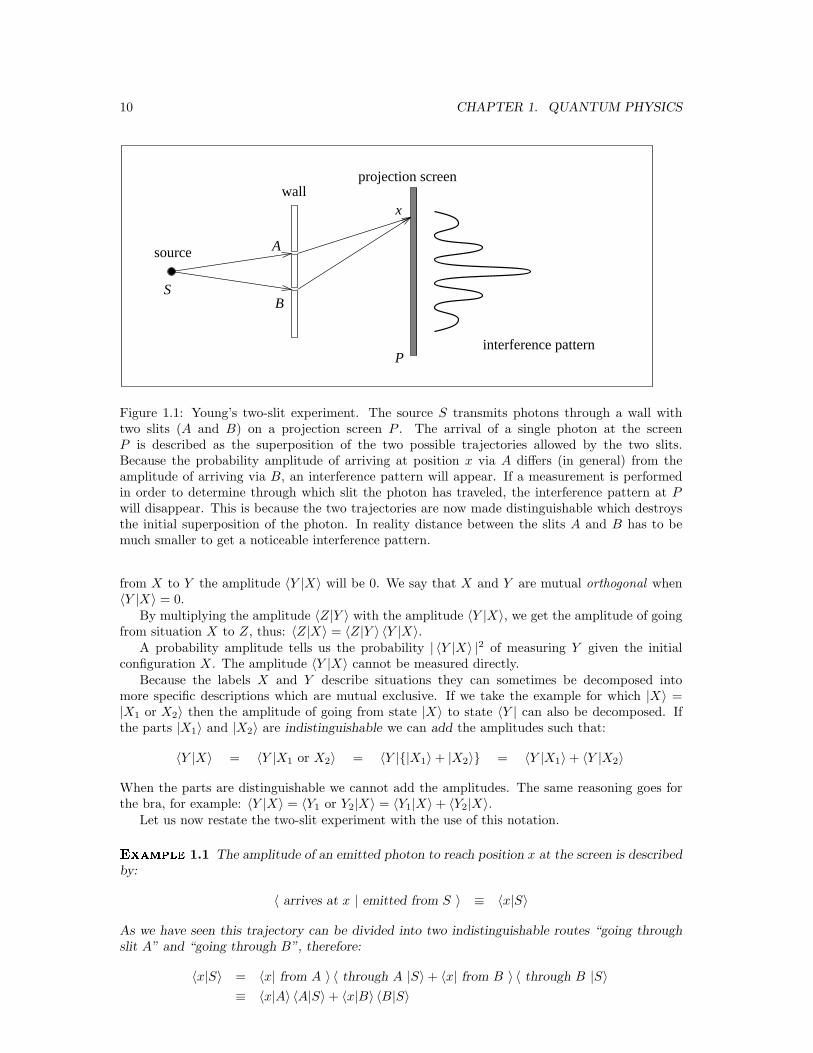
As a start we will look at Young’s two-slit experiment which shows us the basic properties of quan-tum physics (Figure 1.1). After describing this well-known experiment in words, the bracket no-tation will be introduced. The mathematical background of this notational tool will be explained.We refer to the standard introductory books for a more thorough and detailed explanation ofquantum physics [10, 14, 24].
The set-up of the two-slit experiment is as follows. A source S sends a photon through a wallwith two-slits A and B on a projection screen P . The probability of a photon arriving at positionx on this screen will depend on the value of x. When we repeat this experiment for a large numberof photons this probability-distribution on P will produce an interference pattern which can beexplained by the wave-like properties of light.
The problem is that this interference also occurs when the source emits photons at such a lowrate that only one photon at the time travels from S to P . This means that a photon can interferewith itself. To understand this phenomenon we have to look more precise to what is happening.
For every photon that arrives at x there are two possibilities for its history: it either wentthrough slit A or slit B (from the source S). After the photon has been observed at x it isimpossible to determine if it used A or B to pass the wall. We therefore say that the two routes“from S, through A, to x” and “from S, through B, to x” are indistinguishable. This is a necessaryfeature of the experiment because when we do track down the way the photon goes, the interferencepattern vanishes. (This can be done by setting up two detectors at the two slits.) In short: aphoton that goes through specifically one slit cannot interfere with itself.
1.2 The Bra-ket notation
We now know that the interference depends on the set of possible paths a photon can travel fromS to x. This can be described by the bra-ket notation. This is the conventional way of describingquantum mechanical events and was introduced by Paul Dirac [17]. The mathematical basis ofthis formalism will be explained in the next section.
When it is possible to go from a configuration X to configuration Y we can describe this witha non-zero probability amplitude 〈Y |X〉. This amplitude is a complex number with a norm ≤ 1.The 〈Y | part of this expression is called a bra, the |X〉 part is a ket. The whole term is thereforecalled a bra-ket. Inside this bracket are descriptions (note: not mathematical expressions). Abracket should be read from right to left to understand its meaning. If it is not possible to go
9
10 CHAPTER 1. QUANTUM PHYSICS
interference pattern
source
wallprojection screen
S
A
B
x
P
Figure 1.1: Young’s two-slit experiment. The source S transmits photons through a wall withtwo slits (A and B) on a projection screen P . The arrival of a single photon at the screenP is described as the superposition of the two possible trajectories allowed by the two slits.Because the probability amplitude of arriving at position x via A differs (in general) from theamplitude of arriving via B, an interference pattern will appear. If a measurement is performedin order to determine through which slit the photon has traveled, the interference pattern at Pwill disappear. This is because the two trajectories are now made distinguishable which destroysthe initial superposition of the photon. In reality distance between the slits A and B has to bemuch smaller to get a noticeable interference pattern.
from X to Y the amplitude 〈Y |X〉 will be 0. We say that X and Y are mutual orthogonal when〈Y |X〉 = 0.
By multiplying the amplitude 〈Z|Y 〉 with the amplitude 〈Y |X〉, we get the amplitude of goingfrom situation X to Z, thus: 〈Z|X〉 = 〈Z|Y 〉 〈Y |X〉.
A probability amplitude tells us the probability | 〈Y |X〉 |2 of measuring Y given the initialconfiguration X. The amplitude 〈Y |X〉 cannot be measured directly.
Because the labels X and Y describe situations they can sometimes be decomposed intomore specific descriptions which are mutual exclusive. If we take the example for which |X〉 =|X1 or X2〉 then the amplitude of going from state |X〉 to state 〈Y | can also be decomposed. Ifthe parts |X1〉 and |X2〉 are indistinguishable we can add the amplitudes such that:
〈Y |X〉 = 〈Y |X1 or X2〉 = 〈Y |{|X1〉 + |X2〉} = 〈Y |X1〉 + 〈Y |X2〉
When the parts are distinguishable we cannot add the amplitudes. The same reasoning goes forthe bra, for example: 〈Y |X〉 = 〈Y1 or Y2|X〉 = 〈Y1|X〉 + 〈Y2|X〉.
Let us now restate the two-slit experiment with the use of this notation.
�������1.1 The amplitude of an emitted photon to reach position x at the screen is describedby:
〈 arrives at x | emitted from S 〉 ≡ 〈x|S〉
As we have seen this trajectory can be divided into two indistinguishable routes “going throughslit A” and “going through B”, therefore:
〈x|S〉 = 〈x| from A 〉 〈 through A |S〉 + 〈x| from B 〉 〈 through B |S〉≡ 〈x|A〉 〈A|S〉 + 〈x|B〉 〈B|S〉
1.3. THE MATHEMATICS OF QUANTUM PHYSICS 11
The probability of a photon to reach x from S is thus calculated by:
| 〈x|S〉 |2 = | 〈x|A〉 〈A|S〉 + 〈x|B〉 〈B|S〉 |2
This shows how the amplitudes 〈x|A〉 〈A|S〉 and 〈x|B〉 〈B|S〉 can interact and thereby increase or
decrease the value | 〈x|S〉 |2. If the A and B-part have the same phase, the probability is amplified.Take for example the values: 〈x|A〉 〈A|S〉 = 〈x|B〉 〈B|S〉 = 1/2. The probability of a photon to
reach x via A or B individually equals |1/2|2 = 1/4. But the total probability is |1/2 + 1/2|2 = 1.The two parts ‘cancel’ each other out if they have opposite phases. To see this we have to
change 〈x|B〉 〈B|S〉 into −1/2 such that | 〈x|S〉 |2 = 0. This phase-dependent behavior explainsthe interference pattern in our experiment. The phase of a photon to go from a slit to a positionx on the screen depends on the distance between the slit and x. Because the distances A− x andB − x are different for every x, the two amplitudes 〈x|A〉 and 〈x|B〉 sum up differently for everyposition x.
When we make the A and B parts distinguishable (for example by using a photon-detectorat the slits) this expression changes. Because we cannot add the amplitudes 〈x|A〉 〈A|S〉 and〈x|B〉 〈B|S〉 anymore, the probability of measuring a photon at x now equals:
| 〈x|S〉 |2 = | 〈 arrives at x through A |S〉 |2 + | 〈 arrives at x through B |S〉 |2
= | 〈x|A〉 〈A|S〉 |2 + | 〈x|B〉 〈B|S〉 |2
We simply have to add the two probabilities.The difference between the two calculations lies in the fact that amplitudes are complex-valued
numbers but probabilities are always in the domain [0, 1] ⊂ R. 3
1.3 The Mathematics of Quantum Physics
We will now make the bracket notation more precise and meaningful in a mathematical sense.This can be done by defining a complex valued vector space such that the |·〉 and |·〉 expressionsare vectors with an inner product 〈·|·〉. For our purposes it will be sufficient to use the followingtwo definitions of a Hilbertian space and a state space.
����������1.1 (Hilbertian space) For every set of basis states B, the Hilbertian space `2(B)
is the complex-valued linear space on the domain B with a bounded norm. In other words, forevery
X =∑
ξ∈B
αξ · ξ
with αξ ∈ C, the vector X is an element of `2(B) if and only if (α∗ is the complex conjugate ofα ∈ C)
∑
ξ∈B
αξα∗ξ < ∞
This space is equipped with an inner product 〈·, ·〉 : `2(B)×`2(B) → C and a norm ‖·‖ : `2(B) → Rdefined by:
〈X,Y 〉 =
⟨
∑
ξ∈B
αξ · ξ
,
∑
ξ∈B
βξ · ξ
⟩
=∑
ξ∈B
αξβ∗ξ
and ‖X‖ =√
〈X,X〉 for every X,Y ∈ `2(B). By definition all the vectors in B are mutuallyorthogonal and have norm 1.
12 CHAPTER 1. QUANTUM PHYSICS
Note that we do not claim that this is the formal definition of a Hilbert space. The above described`2(·) space is only an example of a Hilbert-space. It can be shown that the inner product andnorm have the properties:
〈X,αY + βZ〉 = α 〈X,Y 〉 + β 〈X,Y 〉 ‖X‖ ≥ 0
〈X,Y 〉 = 〈Y,X〉∗ ‖X‖ = 0 if and only if X = 0
〈X,X〉 ≥ 0 ‖X‖ + ‖Y ‖ ≥ ‖X + Y ‖〈X,X〉 = 0 if and only if X = 0 ‖αX‖ = |α| ‖X‖
for every α, β ∈ C and X,Y,Z ∈ `2(B). Which are exactly the properties we want them to have.The complex-values in combination with the notation of the inner product already forecasts
the next definition which formalizes the bra-ket notation.
����������1.2 (State space) Given a set of basis states B, the state space HB equals the
Hilbertian space `2(B) restricted to the vectors with norm 1. The bracket notation enables us todescribe vectors by 〈X| and |Y 〉 ∈ HB . If we restrict the inner product on `2(B) to the domainHB , we define with this notation:
〈X|Y 〉 ≡ 〈〈X|, |Y 〉〉
The Hilbertian space `2(B) is a complex, linear space spanned by the basis set B. Every vectoris in `2(B) is therefore a linear combination of basis states ∈ B. Because the state space HB isa subset of `2(B), every state |X〉 ∈ HB is also described by a linear combination of basis states.A state does not determine its basis set. It is therefore possible to have two different basis setsA 6= B with HB = HB .
1.4 The Superposition of Basis States
The possible configurations of a physical system are described by the state space HB which isspanned by a set of basis states B. The number of basis states (which equals the dimension ofHB) can be infinite and even uncountable (like the arriving of a photon on a position x ∈ R in ourexample). From now on we will only look at finite dimensional state spaces. A basis state ξ ∈ Bwill be denoted by |ξ〉 to preserve the bracket notation.
As a consequence of this, every state |X〉 can be described by a linear combination on the basisstates B:
|X〉 =∑
ξ∈B
αξ|ξ〉
with α ∈ C. It is said that X is in a superposition of basis states B.Because B is an orthogonal basis set with all vectors norm 1 we have for every ξ, χ ∈ B:
〈χ|ξ〉 =
{1 if χ = ξ0 if χ 6= ξ
By multiplying the linear combination of X on the left with a basis state 〈χ| we therefore get:
〈χ|X〉 =∑
ξ∈B
αξ 〈χ|ξ〉 = αχ
for every χ ∈ B. This shows us how the inner product in the Hilbertian space `2(B) relates to theprobability amplitudes in quantum mechanics and vice versa. By definition is holds that
|X〉 =∑
ξ∈B
|ξ〉 〈ξ|X〉
1.5. EVOLUTION OF QUANTUM MECHANICAL SYSTEMS 13
for every state |X〉 in the state space HB . The probability of measuring a state |X〉 in the basis
state ξ equals | 〈ξ|X〉 |2. By the ‘norm 1’ constraint on the state space HB we see that the overallprobability of measuring a configuration X in a basis state is 1:
∑
ξ∈B
|〈ξ|X〉|2 = 1
for every |X〉 ∈ HB. This is the normalization restriction which will play an eminent role in thisthesis. Only states and transformations which respect this restriction are sensible from a physicalpoint of view. We say that a state space and its transformations have to be proper or well-formed.This normalization condition for HB is a restriction on the Hilbertian space `2(B). The classicalstate space B is a subset of HB where every amplitude has the value 0 or 1. We therefore canwrite:
B ( HB ( `2(B)
1.5 Evolution of Quantum Mechanical Systems
If we want to be more precise about the (time)-evolution a system undergoes, we have to usetransformations which describe this evolution in the state space. The transformations are con-ventionally called operators or time operators. If under the influence of a operator U a systemsevolves from state |X〉 to a state |Y 〉, we denote this by:
U |X〉 = |Y 〉 or 〈Y |U |X〉 = 1 or |X〉 −→U |Y 〉
If we want this operator to obey the laws of quantum mechanics U has to be both linear and normpreserving. It has to respect the normalization condition and the superposition principle of thestate space HB . We therefore can write
U |X〉 = U
∑
ξ∈B
αξ|ξ〉
=∑
ξ∈B
αξ · U |ξ〉
for every |X〉 ∈ HB . Because U is a linear transformation it can be described by a matrix MU .If we want this matrix to be norm preserving it has to be a unitary matrix. In order to defineunitarity we first have to define the hermitian conjugate of a matrix.
����������1.3 (Hermitian conjugate) The hermitian conjugate of a matrix M is the matrix
M† with [M†]ij ≡ [M ]∗ji for every index i and j.
This enables us to define:
����������1.4 (Unitary matrix) A unitary matrix M is a complex valued matrix such that
the hermitian conjugate M† is the inverse of M and vice versa. Therefore:
M · M† = M† · M = I
A unitary transformation is thus defined by a unitary matrix. From now on we will make nodistinction between a function U and the corresponding matrix U .
����������1.5 (Unitary transformation) A transformation U : HB → HB of the statespace HB is unitary if and only if it corresponds to a unitary matrix U ∈ Cd×d with d thedimension of HB .
Because every unitary matrix U has an inverse U† it defines a bijective or reversible transformation.The classical unitary transformations are a subset of the unitary transformations and are describedby the unitary matrices U with [U ]ij ∈ {0, 1} for every i, j. See the appendix for the definition ofa unitary transformation on a infinite dimensional state space.
14 CHAPTER 1. QUANTUM PHYSICS
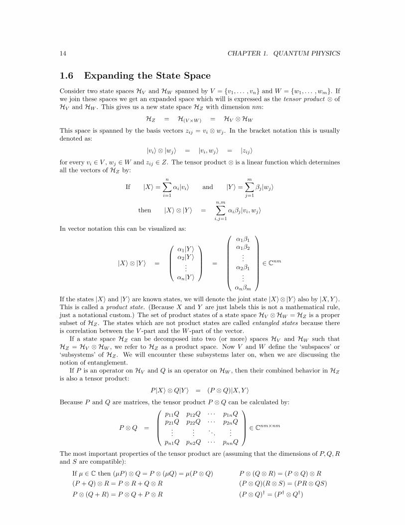
1.6 Expanding the State Space
Consider two state spaces HV and HW spanned by V = {v1, . . . , vn} and W = {w1, . . . , wm}. Ifwe join these spaces we get an expanded space which will is expressed as the tensor product ⊗ ofHV and HW . This gives us a new state space HZ with dimension nm:
HZ = H(V ×W ) = HV ⊗HW
This space is spanned by the basis vectors zij = vi ⊗ wj . In the bracket notation this is usuallydenoted as:
|vi〉 ⊗ |wj〉 = |vi, wj〉 = |zij〉for every vi ∈ V , wj ∈ W and zij ∈ Z. The tensor product ⊗ is a linear function which determinesall the vectors of HZ by:
If |X〉 =
n∑
i=1
αi|vi〉 and |Y 〉 =
m∑
j=1
βj |wj〉
then |X〉 ⊗ |Y 〉 =
n,m∑
i,j=1
αiβj |vi, wj〉
In vector notation this can be visualized as:
|X〉 ⊗ |Y 〉 =
α1|Y 〉α2|Y 〉
...αn|Y 〉
=
α1β1
α1β2
...α2β1
...αnβm
∈ Cnm
If the states |X〉 and |Y 〉 are known states, we will denote the joint state |X〉⊗ |Y 〉 also by |X,Y 〉.This is called a product state. (Because X and Y are just labels this is not a mathematical rule,just a notational custom.) The set of product states of a state space HV ⊗HW = HZ is a propersubset of HZ . The states which are not product states are called entangled states because thereis correlation between the V -part and the W -part of the vector.
If a state space HZ can be decomposed into two (or more) spaces HV and HW such thatHZ = HV ⊗ HW , we refer to HZ as a product space. Now V and W define the ‘subspaces’ or‘subsystems’ of HZ . We will encounter these subsystems later on, when we are discussing thenotion of entanglement.
If P is an operator on HV and Q is an operator on HW , then their combined behavior in HZ
is also a tensor product:
P |X〉 ⊗ Q|Y 〉 = (P ⊗ Q)|X,Y 〉Because P and Q are matrices, the tensor product P ⊗ Q can be calculated by:
P ⊗ Q =
p11Q p12Q · · · p1nQp21Q p22Q · · · p2nQ
......
. . ....
pn1Q pn2Q · · · pnnQ
∈ Cnm×nm
The most important properties of the tensor product are (assuming that the dimensions of P,Q,Rand S are compatible):
If µ ∈ C then (µP ) ⊗ Q = P ⊗ (µQ) = µ(P ⊗ Q) P ⊗ (Q ⊗ R) = (P ⊗ Q) ⊗ R
(P + Q) ⊗ R = P ⊗ R + Q ⊗ R (P ⊗ Q)(R ⊗ S) = (PR ⊗ QS)
P ⊗ (Q + R) = P ⊗ Q + P ⊗ R (P ⊗ Q)† = (P † ⊗ Q†)
1.7. THE EFFECTS OF MEASUREMENT 15
Tensor products for matrices are also called “direct products” or “Kronecker products” [25, 33, 47].The tensor product should not be confused with the Cartesian product “×”. A tensor product oftwo spaces HA and HB is induced by the Cartesian product of the two basis sets A and B.
1.6.1 Notational Customs
The following notational customs will be used in this paper. When necessary, a brief explanationwill be given.
repeated tensor products By P [n] (with n ∈ N+) we mean P ⊗ P ⊗ · · · ⊗ P (n times) and bydefinition P [0] = 1 ∈ C. Because a tensor product does not commute, we have to defineexplicitly:
⊗
i∈Zr
Pi =i=r−1⊗
i=0
Pi = P0 ⊗ P1 ⊗ · · · ⊗ Pr−1
for r ∈ N+, and because P [0] = 1 also:
r−1⊗
i=r
Pi = 1 ∈ C
state space If we use the basis set B, the corresponding state space will be denoted by HB .
basis set/states The set B is will be treated as a subset of HQ. The basis states in B will alsobe named canonical states.
ket notation For every basis state ξ ∈ B we will write |ξ〉 when ξ is used in the context of statespace HB .
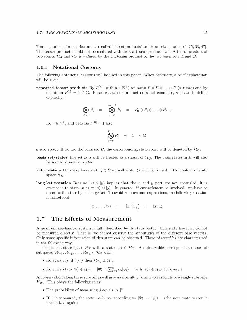
long ket notation Because |x〉 ⊗ |y〉 implies that the x and y part are not entangled, it iserroneous to state |x, y〉 ≡ |x〉 ⊗ |y〉. In general –if entanglement is involved– we have todescribe the state by one large ket. To avoid cumbersome expressions, the following notationis introduced:
|xa, . . . , xb〉 =∣∣∣[xi]
bi=a
⟩
= |xa:b〉
1.7 The Effects of Measurement
A quantum mechanical system is fully described by its state vector. This state however, cannotbe measured directly. That is, we cannot observe the amplitudes of the different base vectors.Only some specific information of this state can be observed. These observables are characterizedin the following way.
Consider a state space HZ with a state |Ψ〉 ∈ HZ . An observable corresponds to a set ofsubspaces HW1
,HW2, . . . ,HWk
⊆ HZ with:
• for every i, j, if i 6= j then HWi⊥ HWj
• for every state |Ψ〉 ∈ HZ : |Ψ〉 =∑k
i=1 αi|ψi〉 with |ψi〉 ∈ HWifor every i
An observation along these subspaces will give us a result ‘j’ which corresponds to a single subspaceHWj
. This obeys the following rules:
• The probability of measuring j equals |αj |2.
• If j is measured, the state collapses according to |Ψ〉 Ã |ψj〉 (the new state vector isnormalized again)
16 CHAPTER 1. QUANTUM PHYSICS
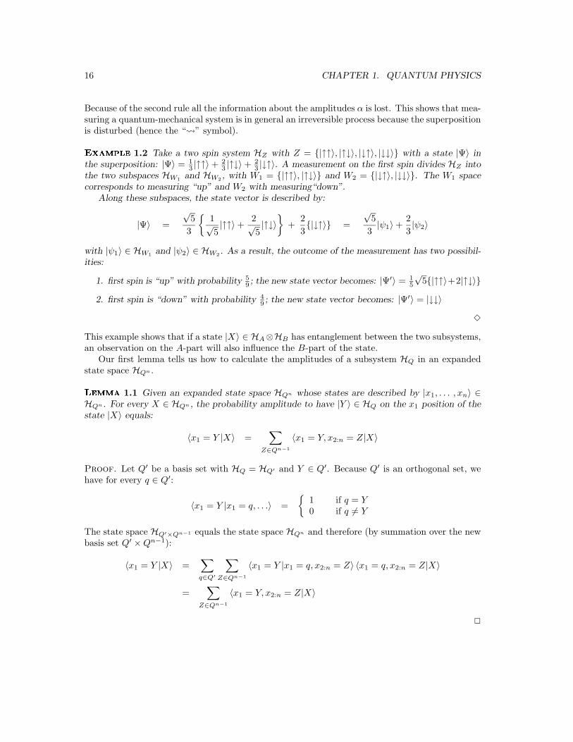
Because of the second rule all the information about the amplitudes α is lost. This shows that mea-suring a quantum-mechanical system is in general an irreversible process because the superpositionis disturbed (hence the “Ô symbol).
�������
1.2 Take a two spin system HZ with Z = {|↑↑〉, |↑↓〉, |↓↑〉, |↓↓〉} with a state |Ψ〉 inthe superposition: |Ψ〉 = 1
3 |↑↑〉 + 23 |↑↓〉 + 2
3 |↓↑〉. A measurement on the first spin divides HZ intothe two subspaces HW1
and HW2, with W1 = {|↑↑〉, |↑↓〉} and W2 = {|↓↑〉, |↓↓〉}. The W1 space
corresponds to measuring “up” and W2 with measuring“down”.Along these subspaces, the state vector is described by:
|Ψ〉 =
√5
3
{1√5|↑↑〉 +
2√5|↑↓〉
}
+2
3{|↓↑〉} =
√5
3|ψ1〉 +
2
3|ψ2〉
with |ψ1〉 ∈ HW1and |ψ2〉 ∈ HW2
. As a result, the outcome of the measurement has two possibil-ities:
1. first spin is “up” with probability 59 ; the new state vector becomes: |Ψ′〉 = 1
5
√5{|↑↑〉+2|↑↓〉}
2. first spin is “down” with probability 49 ; the new state vector becomes: |Ψ′〉 = |↓↓〉
3
This example shows that if a state |X〉 ∈ HA⊗HB has entanglement between the two subsystems,an observation on the A-part will also influence the B-part of the state.
Our first lemma tells us how to calculate the amplitudes of a subsystem HQ in an expandedstate space HQn .
�����1.1 Given an expanded state space HQn whose states are described by |x1, . . . , xn〉 ∈
HQn . For every X ∈ HQn , the probability amplitude to have |Y 〉 ∈ HQ on the x1 position of thestate |X〉 equals:
〈x1 = Y |X〉 =∑
Z∈Qn−1
〈x1 = Y, x2:n = Z|X〉
Proof. Let Q′ be a basis set with HQ = HQ′ and Y ∈ Q′. Because Q′ is an orthogonal set, wehave for every q ∈ Q′:
〈x1 = Y |x1 = q, . . .〉 =
{1 if q = Y0 if q 6= Y
The state space HQ′×Qn−1 equals the state space HQn and therefore (by summation over the newbasis set Q′ × Qn−1):
〈x1 = Y |X〉 =∑
q∈Q′
∑
Z∈Qn−1
〈x1 = Y |x1 = q, x2:n = Z〉 〈x1 = q, x2:n = Z|X〉
=∑
Z∈Qn−1
〈x1 = Y, x2:n = Z|X〉
2
Chapter 2
Quantum Computing
In this chapter we will describe the basics of quantum computation. This is done bydefining quantum bits, quantum registers and quantum gates. The model of quantumTuring-machines will also be mentioned.
2.1 Quantum Memory
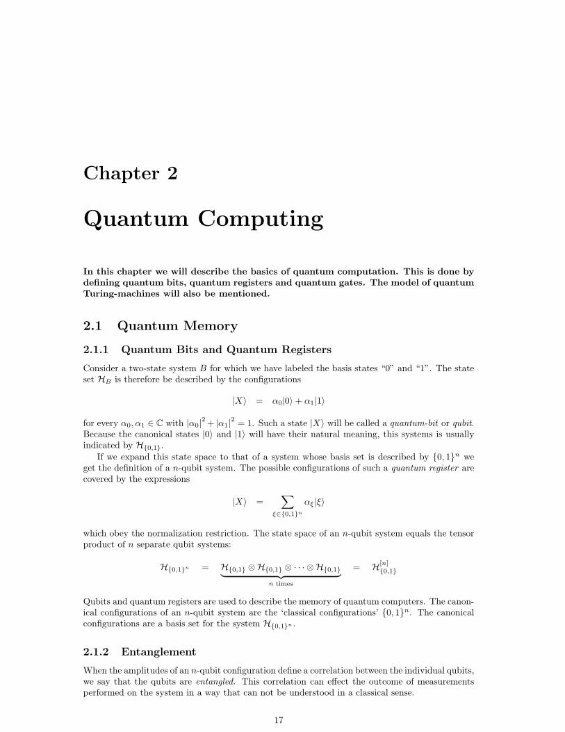
2.1.1 Quantum Bits and Quantum Registers
Consider a two-state system B for which we have labeled the basis states “0” and “1”. The stateset HB is therefore be described by the configurations
|X〉 = α0|0〉 + α1|1〉
for every α0, α1 ∈ C with |α0|2 + |α1|2 = 1. Such a state |X〉 will be called a quantum-bit or qubit.Because the canonical states |0〉 and |1〉 will have their natural meaning, this systems is usuallyindicated by H{0,1}.
If we expand this state space to that of a system whose basis set is described by {0, 1}n weget the definition of a n-qubit system. The possible configurations of such a quantum register arecovered by the expressions
|X〉 =∑
ξ∈{0,1}n
αξ|ξ〉
which obey the normalization restriction. The state space of an n-qubit system equals the tensorproduct of n separate qubit systems:
H{0,1}n = H{0,1} ⊗H{0,1} ⊗ · · · ⊗ H{0,1}︸ ︷︷ ︸
n times
= H[n]{0,1}
Qubits and quantum registers are used to describe the memory of quantum computers. The canon-ical configurations of an n-qubit system are the ‘classical configurations’ {0, 1}n. The canonicalconfigurations are a basis set for the system H{0,1}n .
2.1.2 Entanglement
When the amplitudes of an n-qubit configuration define a correlation between the individual qubits,we say that the qubits are entangled. This correlation can effect the outcome of measurementsperformed on the system in a way that can not be understood in a classical sense.
17
18 CHAPTER 2. QUANTUM COMPUTING
�������
2.1 Take the following configuration of a two-qubit system:
|Ψ〉 =1
2
√2{|0, 0〉 + |1, 1〉}
When we measure the value of the first qubit, the wave function will collapse to one of the twopossible states:
|Ψ0〉 = |0, 0〉 or |Ψ1〉 = |1, 1〉
This means that the value of the second bit is determined by the outcome of our measurementon the first bit: there is a correlation between the bits. This is not always the case. If the initialtwo-qubit system is a tensor product of two individual qubits, then a measurement on the first bitdoes not affect the second bit. For example:
|Ψ〉 =1
2{|0, 0〉 + |0, 1〉 + |1, 0〉 + |1, 1〉} =
1
2{|01〉 + |11〉} ⊗ {|02〉 + |12〉}
An observation on the first bit changes the system into one of the configurations:
|Ψ0〉 = |01〉 ⊗1
2
√2{|02〉 + |12〉} or |Ψ1〉 = |11〉 ⊗
1
2
√2{|02〉 + |12〉}
which does not affect the second bit. 3
The notion of entanglement is important because it illustrates the influence of a measurementon the system and is typical for quantum-mechanical systems. It also enables the occurrence ofinterference in a quantum computer which defines the fundamental difference between probabilisticand quantum computing.
Entanglement can not always be seen by the probability of measuring certain basis states. Asa counterexample: the two qubits in the following state are entangled:
|Ψ〉 =1
2{|0, 0〉 + |0, 1〉 + |1, 0〉 − |1, 1〉}
although there is no ‘correlation’ to be found when measuring the bits.
2.2 Quantum Gates
We will now look at gates which operate on qubits: quantum gates. In the previous chapter wediscussed unitary transformations operating on a state space. A quantum gate is a system thatperforms such a proper transformation on a register of qubits. Every proper quantum gate thatoperates on a n-qubit system is therefore described by a unitary matrix M ∈ Cd×d (with d = 2n
the dimension of the state space H{0,1}n). An example of a gate that operates on one qubit is thenot-gate.
�������2.2 The not-gate is described by the unitary matrix which operates on the twodimensional state space H{0,1} with
(10
)
≡ |0〉 and
(01
)
≡ |1〉
The matrix Mnot therefore equals
Mnot =
(0 11 0
)
2.2. QUANTUM GATES 19
The ‘traditional’ behavior not(0) = 1 and not(1) = 0 is shown by the matrix multiplications:
Mnot|0〉 =
(0 11 0
)
·(
10
)
=
(01
)
= |1〉
and
Mnot|1〉 =
(0 11 0
)
·(
01
)
=
(10
)
= |0〉
In general we have for this gate:
Mnot{α0|0〉 + α1|1〉} =
(0 11 0
)
·(
α0
α1
)
=
(α1
α0
)
= α1|0〉 + α0|1〉
with α0, α1 ∈ C and |α0|2 + |α1|2 = 1. 3
The last equation in this example shows that a quantum gate has to respect the possible super-position of a quantum register. This enables us to define gates whose behavior is impossible withclassical gates. An example of such a true quantum gate is the following:
�������2.3 Define a one-qubit gate Q by:
Q =1
2
(1 − i 1 + i1 + i 1 − i
)
When applying this gate to the canonical states |0〉 and |1〉, we get: (λ = 12 − i
2 ; |λ|2 = 12 )
Q|0〉 = λ|0〉 + λ∗|1〉 and Q|1〉 = λ∗|0〉 + λ|1〉
In both cases the result is a perfect ‘fifty-fifty’ mixture of |0〉 and |1〉 (there is only a phase differencebetween Q|0〉 and Q|1〉). If we apply the Q-gate a second time on this result we get:
Q{Q|0〉} = |1〉 and Q{Q|1〉} = |0〉
which is the not-function again. This is affirmed by the matrix of Q2:
Q2 =
(0 11 0
)
We therefore say that Q is the “square root of not”. Although the input and output of Q2
‘classical’ it is not possible to have a classical gate Q with the same behavior. This is proven by:det(Q)2 = det(not) = −1 and thus det(Q) ∈ {i,−i} which is impossible for a classical gate. 3
The reversible gates with classical behavior are a proper subset of all possible quantum gates.Non-reversible gates are not proper because the corresponding matrix has to be an invertiblematrix (M · M† = 1).
2.2.1 Proper Quantum Gates
It is not always obvious if a gate is well-formed or not. We therefore will use the following ‘rule ofthumb’ to certify that a gate with a certain requested behavior is proper.
����������2.1 (Requested behavior) The requested behavior of a gate M is described by a
finite list of input and output values 〈(x1, y1), . . . , (xk, yk)〉 such that M(xi) = yi for every i.
This definition is used in the next lemma about proper quantum gates.
20 CHAPTER 2. QUANTUM COMPUTING
�����2.1 If the requested behavior of a gate M : HBn → HBn is described by a list
〈(x1, y1), . . . , (xk, yk)〉
with xi ⊥ xj and yi ⊥ yj for every i 6= j, then there exists a proper quantum gate with M(xi) = yi
for every 1 ≤ i ≤ k.Proof. Let the set of basis states be denoted by Bn = {ξ1, . . . }. Because x1, . . . , xk are mutuallyorthonormal, there exists a unitary transformation P : HBn → HBn with P (ξi) = xi, for every1 ≤ i ≤ k. For the same reason there also exists a unitary R such that R(ξi) = yi. If we defineM = R · P †, M will also be unitary, with for every 1 ≤ i ≤ k: M(xi) = R(P †(xi)) = R(ξi) = yi.
2
2.3 Quantum Gate Circuits
An acyclic circuit of quantum gates is called a quantum (gate) circuit or quantum gate array.The general behavior of a quantum circuit can be calculated with the matrix formalism in astraightforward way.
Consider two gates A and B that operate on two disjoint subsystems of n and m bits:
A : H{0,1}n → H{0,1}n and B : H{0,1}m → H{0,1}m
The combination of A and B defines a transformation on the state space H{0,1}n ⊗ H{0,1}n =H{0,1}n+m described by the tensor product A ⊗ B
(A ⊗ B) : H{0,1}n+m −→ H{0,1}n+m
with
(A ⊗ B)|X,Y 〉 7−→ A|X〉 ⊗ B|Y 〉
for every X ∈ {0, 1}n and Y ∈ {0, 1}m.When two layers of gates act as a sequence on an n-qubit system, the general transformation is
calculated by the product of the two defining matrices. This rule was already used in the exampleof the square root of not gate. To summarize:
1. When two gates are sequential, multiply the matrices
2. When two gates are parallel, take the tensor product of the matrices.
See Figure 2.1 for an example of a small quantum circuit. The characteristics of the quantumcircuit model were first investigated in articles by David Deutsch [16] and Andrew Chi-Chih Yao[60].
2.3.1 A Universal Quantum Gate
Because quantum arrays define unitary transformations on qubit systems, it is natural to ask“What kind of quantum gates do we need to implement an arbitrary unitary transformation?”For classical non-reversible computation we know that it is sufficient to have and, or and not-gates. The quantum case is a more difficult problem to solve.
It is impossible to construct every unitary transformation exactly with a finite set of basic gatesbecause the number of possible transformations is uncountable. We therefore have to approximatethe transformation within a bounded error. This means that given a transformation U and anarbitrary small number ε > 0 we can make a circuit U ′ which simulates U within the allowederror ε, that is ‖U − U ′‖ ≤ ε. If there exists a quantum gate by which we can construct anytransformation within a bounded error, we will call this gate a universal gate.

2.4. QUANTUM TURING MACHINES 21
A CB
D E
layer with gates:
layer with gates:
A,B,C
D,E
Figure 2.1: A small quantum gate circuit with two layers and five gates. The action of the firstlayer is described by the tensor product A ⊗ B ⊗ C. The second layer equals: D ⊗ E. Thetransformation defined by this circuit is therefore described by: (D ⊗ E) · (A ⊗ B ⊗ C).
It was proven by David Deutsch that there exists a universal gate that operates on three bits[16]. After that, Adriano Barenco[3] and David DiVincenzo[18] showed the existence of a two bitgate which is universal in is computational power. For a detailed expose of this subject the readeris best referred to the famous ‘article by nine authors’ by Adriano Barenco et al. The quantumcircuit model has proven to be the most convenient model to study quantum computing.
2.4 Quantum Turing Machines
The quantum Turing machine provides us with an alternative model for quantum computing.There is strong relationship between the characteristics of such qtms and reversible Turing ma-chines [5, 15]. The following definition has its origin by Ethan Bernstein and Umesh Vazirani[6].
����������2.2 (Quantum Turing machine) A Quantum Turing Machine M is defined by
the tuple 〈K,Σ, δ〉, with Σ a finite alphabet set (including a blank symbol ¤), K a finite internalstate set and δ : K × Σ × {←,→}× K × Σ → C the finite state control.
The set of basis states is described by the states |Ψ〉 = |k, h, ψ〉 ∈ `2(K × N × Q∗) = S, where kindicates the internal state of the qtm; h defines the head-position on the one-way infinite tapeand ψ describes the tape-content (with only a finite number of non-blank symbols). The globaltransition function M : S → S now obeys (for every k, h, ψ, q, h′, k′ and ψ′):
〈k′, h − 1, ψ0:h−1 × q × ψh+1:...|M |k, h, ψ〉 = δ(k, ψh,←, q, k′)
〈k′, h + 1, ψ0:h−1 × q × ψh+1:...|M |k, h, ψ〉 = δ(k, ψh,→, q, k′)
〈k′, h′, ψ′|M |k, h, ψ〉 = 0 otherwise
(Note that by each computational step the head must move.) By superposition on the set ofbasis states, M describes a transformation on the Hilbertian space S. If M describes a unitarytransformation, the qtm M is said to be well formed or proper.
��������2.1 We will use the following notational conventions: (|X〉, |Y 〉 ∈ S and M a wellformed qtm):
• Instead of |k, h, ψ〉 we may also write |k, ψ0, . . . , ψh−1, ψh, ψh+1, . . .〉.
• By |X〉 −→M |Y 〉 we mean: M |X〉 = |Y 〉
• If there exists a t ∈ N with M t|X〉 = |Y 〉 we denote this by |X〉 ∗−→M |Y 〉
22 CHAPTER 2. QUANTUM COMPUTING
• The internal state is often described by a function-value p. . .q. For example, with pstartqand phaltq we mean the starting and halting state ∈ K of the qtm. This is done withoutfurther specification.
2.4.1 Well Formed ���s
Because qtms will not play an important role in this paper, we will only summarize the maincharacteristics of quantum Turing machines. First of all we have to take a closer look at the wellformedness issue. To handle this restriction on the infinite dimensional Hilbertian space S, EthanBernstein and Umesh Vazirani translated it into the following three constraints.
�����2.2 A quantum Turing machine is well formed if and only if the finite state control δ
obeys the following local conditions (where∑
k,h,ψ |k, h, ψ〉 describes the summation on the basisstates of S):
1. For every basis state X, the transformation M is norm preserving:
∑
k,h,ψ
|〈k, h, ψ|M |X〉|2 = 1
2. If X and Y are different basis states with identical head positions, then M(X) and M(Y )are orthogonal:
∑
k,h,ψ
〈Y |M |k, h, ψ〉〈k, h, ψ|M |X〉 = 0
3. For every basis state X with head position h the ‘←’ and ‘→’-part are mutual orthogonal:
∑
k,ψ
〈k, h + 1, ψ|M |X〉〈X|M |k, h − 1, ψ〉 = 0
Proof. See the original paper [6]. 2
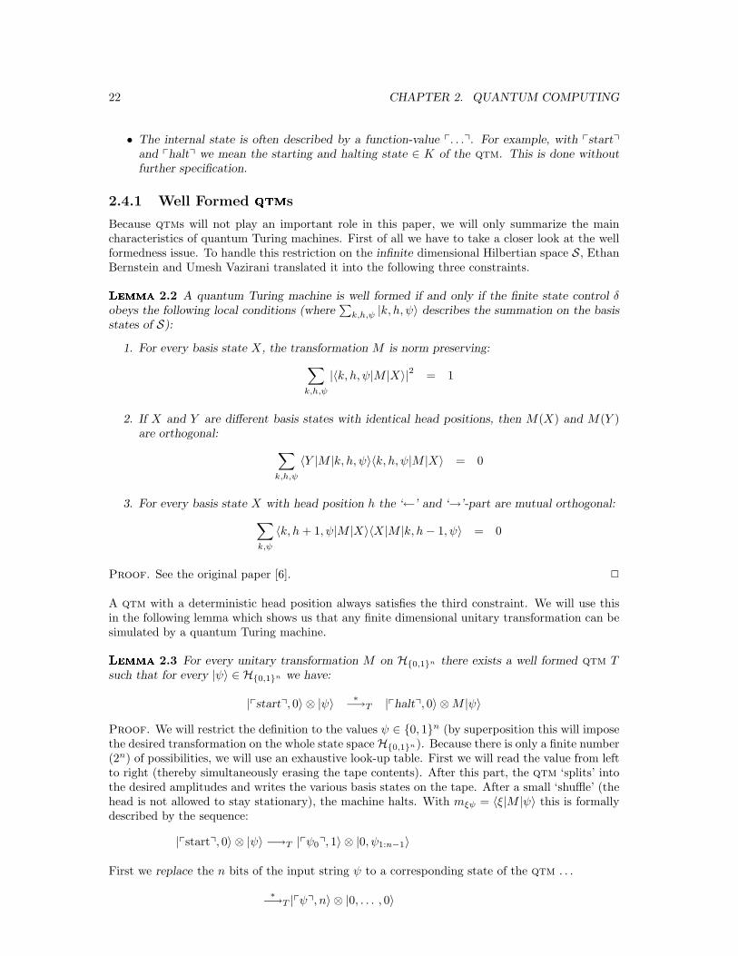
A qtm with a deterministic head position always satisfies the third constraint. We will use thisin the following lemma which shows us that any finite dimensional unitary transformation can besimulated by a quantum Turing machine.
�����2.3 For every unitary transformation M on H{0,1}n there exists a well formed qtm T
such that for every |ψ〉 ∈ H{0,1}n we have:
|pstartq, 0〉 ⊗ |ψ〉 ∗−→T |phaltq, 0〉 ⊗ M |ψ〉
Proof. We will restrict the definition to the values ψ ∈ {0, 1}n (by superposition this will imposethe desired transformation on the whole state space H{0,1}n). Because there is only a finite number(2n) of possibilities, we will use an exhaustive look-up table. First we will read the value from leftto right (thereby simultaneously erasing the tape contents). After this part, the qtm ‘splits’ intothe desired amplitudes and writes the various basis states on the tape. After a small ‘shuffle’ (thehead is not allowed to stay stationary), the machine halts. With mξψ = 〈ξ|M |ψ〉 this is formallydescribed by the sequence:
|pstartq, 0〉 ⊗ |ψ〉 −→T |pψ0q, 1〉 ⊗ |0, ψ1:n−1〉
First we replace the n bits of the input string ψ to a corresponding state of the qtm . . .
∗−→T |pψq, n〉 ⊗ |0, . . . , 0〉
2.5. ALGORITHMS FOR QUANTUM COMPUTERS 23
after which the output value is calculated by a finite look-up table. This produces a superpositionon the internal state of the qtm with amplitudes m.
−→T
∑
ξ∈{0,1}n
mξψ|pψ, ξq, n − 1〉 ⊗ |0, . . . , 0〉
By moving the head backwards, this output string is written on the tape of the Turing machine.
−→T
∑
ξ∈{0,1}n
mξψ|pψ, ξ0:n−2q, n − 2〉 ⊗ |0, . . . , 0, ξn−1〉
By doing so, the superposition of the machine T is transported to a superposition on the tape,
∗−→T
∑
ξ∈{0,1}n
mξψ|pψ, ξ0q, 0〉 ⊗ |0, ξ1:n−1〉
Finally, the qtm is returns to one basis state ‘halting . . . ’ which shuffles the head one last time.
−→T
∑
ξ∈{0,1}n
|phalting . . . q, 1〉 ⊗ mξψ|ξ〉
−→T |phaltq, 0〉 ⊗ M |ψ〉With lemma 2.2 and the unitarity of M we can verify the well formedness of this qtm. BecauseM is norm preserving, the m values will also be proper (requirement 1). The p. . .q-function willbe defined in such a way that ψ 6= ψ′ implies |pψq〉 ⊥ |pψ′
q〉. The transformation M is anglepreserving, and therefore M |ψ〉 ⊥ M |ψ′〉 which certifies the second restriction. Because this qtm
has deterministic head position, the third requirement is trivial. 2
It was shown by Ethan Bernstein and Umesh Vazirani[6] that there exists a Universal qtm thatcan simulate any other qtm with only polynomial slowdown. The equivalence of the quantumcircuit model and qtm-model was proven by Andrew Chi-Chih Yao[60].
2.5 Algorithms for Quantum Computers
What are quantum computers good for? When we want to simulate a quantum mechanical systema quantum computer could be very useful. On a classical computer we would have to computethe evolution for every basis state after which the final result is obtained by a summation of thecalculated amplitudes for each basis state. For an n dimensional state space this calculation has atime complexity proportional to n. Because the dimension of the state space grows exponentiallyin the size of the system, this is a time consuming procedure. With a quantum computer thisproblem of large state spaces is solved by allowing the quantum computer to enter an equally sizedsuperposition. By doing this we do not have to do the calculation for every basis state becausethe computer does this in parallel. This ‘quantum parallelism’ is also the main idea behind thealgorithms that have been constructed to solve traditional computational problems in a faster waythan is possible (or known to be possible) on a classical computer.
�������2.4 Assume a function f : {0, 1}n → {0, 1} and a quantum algorithm M with
M |ξ, 0〉 = |ξ, f(ξ)〉for every ξ ∈ {0, 1}n. If we provide this algorithm with an equally distributed superpositionof input states, we can calculate the superposition of outputs with the same time and spacecomplexity by:
M
∑
ξ∈{0,1}n
2−n/2|ξ, 0〉
=∑
ξ∈{0,1}n
2−n/2|ξ, f(ξ)〉
24 CHAPTER 2. QUANTUM COMPUTING
A measurement on this superposition gives us one of the basis states |ξ, f(ξ)〉 with a probability of2−n. Because we cannot control the probabilities of a measurement it would be misleading to saythat we really ‘know’ all the possible outcomes of a function. In general it is impossible to forcethe superposition into a basis state with f(ξ) = 1. In order to take advantage of this superpositionwe have to use the interference phenomenon on the amplitudes of the basis states [7, 22, 30, 51].If this is possible and how to do this depends on the function f we have calculated. 3
In 1994 Peter Shor showed how a quantum computer could be used to factor numbers with onlypolynomial time complexity [49, 50]. Not only does this algorithm decide if a number is prime ornot but it will also give the prime factors of a composite number. It is generally believed but notknown that on a classical computer this problem requires an exponential amount of time to solve.Moreover, because of this intractability, factorization is commonly used in modern encryptionschemes such as RSA.
Another result was achieved more recently by Lov Grover [26, 9]. He proved that for anyfunction f : Zn → {0, 1} it possible to find a number i with f(i) = 1 (if such a number exists)with a time complexity proportional to
√n. This quantum searching algorithm does not assume
any knowledge about the function f . Although this is not an exponential speed-up it is likely thatevery deterministic or probabilistic algorithm will have a time complexity proportional to n forthis task.
Chapter 3
Classical Cellular Automata
In this section we will give a brief description of cellular automata and its character-istics. Special attention will be paid to the subclass of reversible cellular automatawhich play an important role in the the theory of quantum cellular automata.
3.1 Cellular Automata
The model of cellular automata (ca) is used to describe the behavior of discrete systems witha uniform and parallel space/time behavior. Given a space S and a local state set Q, a ca willdescribe a function FS : QS → QS which defines the time-evolution of an initial configurationX ∈ QS . Consequently, the configuration at time t ∈ N is described by the expression F t(X).
Before giving a formal definition we will first look at a typical example of a one-dimensionalcellular automaton to make ourselves familiar with some important characteristics.
�������3.1 Consider a one-dimensional, two-state ca F such that the successor X ′ of aconfiguration X ∈ {0, 1}Z is determined by a local function f according to:
X ′ = FZ(X)
= FZ
(⊗
i∈Z
Xi
)
=⊗
i∈Z
f(Xi−1,Xi,Xi+1)
This local function f : Q3 → Q is defined by a finite table:
f(0, 0, 0) = 0 f(0, 0, 1) = 1f(0, 1, 0) = 0 f(0, 1, 1) = 1f(1, 0, 1) = 0 f(1, 0, 0) = 1f(1, 1, 1) = 0 f(1, 1, 0) = 1
which implements the addition-modulo-two-rule: f(x−1, x0, x1) = x−1 ⊕ x1.If we unfold the time parameter t of the global function F t
Zas an additional space-dimension,
we get a (1 + 1)-dimensional structure which shows us the space/time behavior Z×N → Q of theca on an initial configuration X:
(i, t) 7→[F t
Z(X)
]
i
Figure 3.1 shows us the result of this transformation. With the convention that time is goingdownwards each time-step can be identified as a layer in such a structure.
25
26 CHAPTER 3. CLASSICAL CELLULAR AUTOMATA
f
f
f
f
f
f
f
f
f
f
cell values at time t
cell values at time t+1
local functions
local functions
neighborhood scheme
neighborhood scheme
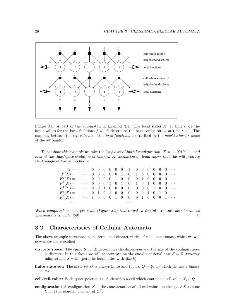
Figure 3.1: A part of the automaton in Example 3.1. The local states Xi at time t are theinput values for the local functions f which determine the next configuration at time t + 1. Themapping between the cell-values and the local functions is described by the neighborhood schemeof the automaton.
To continue this example we take the ‘single seed’ initial configuration: X = · · · 00100 · · · andlook at the time/space evolution of this ca. A calculation by hand shows that this will producethe triangle of Pascal modulo 2:
X = · · · 0 0 0 0 0 0 1 0 0 0 0 0 0 · · ·F (X) = · · · 0 0 0 0 0 1 0 1 0 0 0 0 0 · · ·
F 2(X) = · · · 0 0 0 0 1 0 0 0 1 0 0 0 0 · · ·F 3(X) = · · · 0 0 0 1 0 1 0 1 0 1 0 0 0 · · ·F 4(X) = · · · 0 0 1 0 0 0 0 0 0 0 1 0 0 · · ·F 5(X) = · · · 0 1 0 1 0 0 0 0 0 1 0 1 0 · · ·F 6(X) = · · · 1 0 0 0 1 0 0 0 1 0 0 0 1 · · ·
· · · · · ·
When computed on a larger scale (Figure 3.2) this reveals a fractal structure also known as‘Sierpenski’s triangle’ [59]. 3
3.2 Characteristics of Cellular Automata
The above example mentioned some terms and characteristics of cellular automata which we willnow make more explicit.
discrete space: The space S which determines the dimension and the size of the configurationsis discrete. In this thesis we will concentrate on the one-dimensional case S = Z (two-wayinfinite) and S = Zk (periodic boundaries with size k).
finite state set: The state set Q is always finite and typical Q = {0, 1} which defines a binaryca.
cell/cell-value: Each space-position i ∈ S identifies a cell which contains a cell-value Xi ∈ Q.
configuration: A configuration X is the concatenation of all cell-values on the space S at timet, and therefore an element of QS .
3.3. FORMAL DEFINITION OF CELLULAR AUTOMATA 27
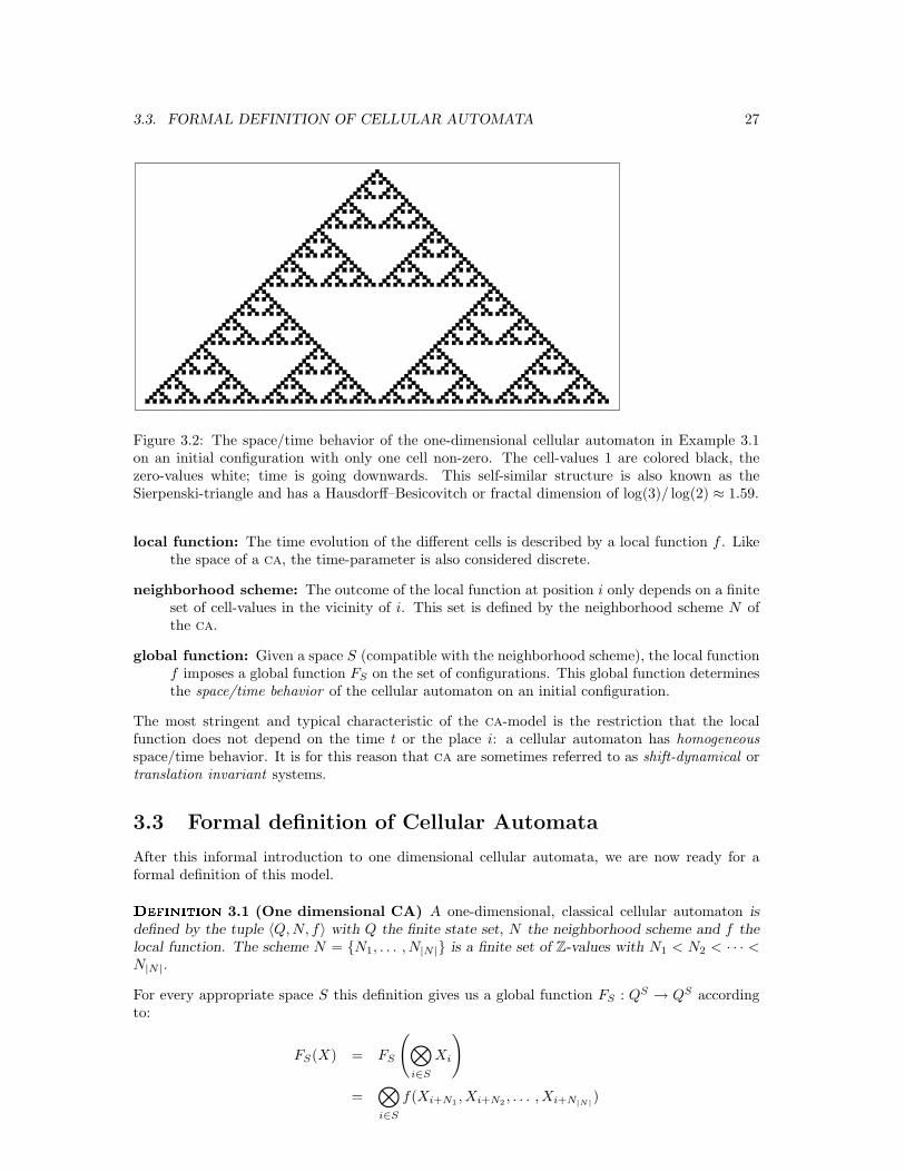
Figure 3.2: The space/time behavior of the one-dimensional cellular automaton in Example 3.1on an initial configuration with only one cell non-zero. The cell-values 1 are colored black, thezero-values white; time is going downwards. This self-similar structure is also known as theSierpenski-triangle and has a Hausdorff–Besicovitch or fractal dimension of log(3)/ log(2) ≈ 1.59.
local function: The time evolution of the different cells is described by a local function f . Likethe space of a ca, the time-parameter is also considered discrete.
neighborhood scheme: The outcome of the local function at position i only depends on a finiteset of cell-values in the vicinity of i. This set is defined by the neighborhood scheme N ofthe ca.
global function: Given a space S (compatible with the neighborhood scheme), the local functionf imposes a global function FS on the set of configurations. This global function determinesthe space/time behavior of the cellular automaton on an initial configuration.
The most stringent and typical characteristic of the ca-model is the restriction that the localfunction does not depend on the time t or the place i: a cellular automaton has homogeneousspace/time behavior. It is for this reason that ca are sometimes referred to as shift-dynamical ortranslation invariant systems.
3.3 Formal definition of Cellular Automata
After this informal introduction to one dimensional cellular automata, we are now ready for aformal definition of this model.
����������3.1 (One dimensional CA) A one-dimensional, classical cellular automaton is
defined by the tuple 〈Q,N, f〉 with Q the finite state set, N the neighborhood scheme and f thelocal function. The scheme N = {N1, . . . , N|N |} is a finite set of Z-values with N1 < N2 < · · · <N|N |.
For every appropriate space S this definition gives us a global function FS : QS → QS accordingto:
FS(X) = FS
(⊗
i∈S
Xi
)
=⊗
i∈S
f(Xi+N1,Xi+N2
, . . . ,Xi+N|N|)
28 CHAPTER 3. CLASSICAL CELLULAR AUTOMATA
To simplify the above notation we introduce the following short hands for the terms appearing inthe local function.
��������3.1 If N = (N1, . . . , N|N |) is a neighborhood scheme it will be understood that:
(Xi+N ) ≡(Xi+N1
,Xi+N2, . . . ,Xi+N|N|
)
and
(Xa:b) ≡ (Xa,Xa+1, . . . ,Xb)
This leads us to the the brief and elementary expression:
F
(⊗
i∈S
Xi
)
=⊗
i∈S
f(Xi+N )
Notice that a ca F = 〈Q,N, f〉 does not determine the space S it is supposed to act on.
�������3.2 The ca of Example 3.1 is described by the tuple F = 〈{0, 1}, (−1, 0, 1), f〉 withf(x, y, z) = x ⊕ z. 3
Because the definition of a neighborhood scheme N does not determine the space S it acts on,we can apply the same ca F = 〈Q,N, f〉 on different structures compatible with the set Z.. Ourmain interest goes to the simple one-dimensional cases Z and Zk which results in the functionsFZ : QZ → QZ and Fk : Qk → Qk with k ∈ N+.
If the neighborhood N does not allow any interaction between the cell-values, the ca will havetrivial behavior. Typically this is the case if |N | = 1. On the other hand it can been shown thatevery ca F can be redefined as a ca with N = {0, 1} without loss of generality. This will beproven in Lemma 6.5.
3.3.1 The Cellular Automata Model
Cellular automata were first used as such by John von Neumann [12, 46]. He showed the possibilityof a universal two dimensional ca. Although not hard to prove, we will only refer the standardliterature for a proof that one-dimensional ca can simulate Turing machines and are thereforecomputational universal. Because of their simple and homogeneous and parallel structure, cellularautomata are frequently used to model physical systems such as gases, liquids et cetera. This,in combination with its use as a mathematical abstraction of parallel computation, makes it aunique combination of physics and theoretical computer science. The last decade there has beena growing interest in theory of cellular automata by computer scientists and physicists because ofthe possibility to simulate large ca with the use of modern computer technology. The articles byStephen Wolfram [58, 59], Tommaso Toffoli [53, 23], Norman Margolus [54], and Howard Gutowitz[27] are a good starting point to investigate this modern use of cellular automata.
3.4 Reversible Cellular Automata
Given a global function F : QZ → QZ, we say that the ca F is global reversible if and only if everyconfiguration Y ∈ QZ has one predecessor X such that: F (X) = Y . A simple reversible cellularautomaton (rca) is described by: k = 2, N = {0, 1} and the local function f with: f(x0, x1) = x0
for every x0, x1 ∈ Q. This rca is just the identity ca with F (X) = X for every X ∈ QZ. Bythis example we see that it is possible to have a rca with a non-reversible local function (whichis always the case with k ≥ 2). More complex rca are also possible but appear to be very rareamong the set of plain cellular automata.
The characteristics of reversible cellular automata are extensively described in a review articleby Tommaso Toffoli and Norman Margolus [27, 52]. For a long time it was unknown if there exists
3.4. REVERSIBLE CELLULAR AUTOMATA 29
a reversible cellular automata capable of embedding a general purpose computer. In 1976 however,Tommaso Toffoli proved that any d-dimensional cellular automaton could be simulated by a d+1-dimensional reversible cellular automaton [52]. By the existence of a universal Turing machineembedded in a 1-dimensional cellular automaton, this proves that there exists a 2-dimensionalreversible cellular automaton which is capable of doing the same. After that Morita and Haraoproved the existence of a one dimensional rca which is universal in its computational power[19, 44, 45]. They did this by defining a special subclass of ca which are reversible by definition:partitioned cellular automata. This type of ca will also be discussed in this thesis.
The ‘modern approach’ to cellular automata with the use of computer simulations seems tosuggest that the old articles on this subject are outdated. Especially for the model of reversibleautomata this not the case. The theory of cellular automata as a computational model is amathematical theory. To avoid ‘re-inventing the wheel’ one should also pay attention to the moreabstract articles by Serafino Amoroso et al. [2], Gustav Hedlund [28], and Daniel Richardson [48].
Chapter 4
Quantum Cellular Automata
In this section we will define the model of one dimensional quantum cellular automata.This model is a straightforward extension of the classical model that exists for onedimensional
��.
4.1 The Size of the State Space
Before we describe the various models a note must be made on the size of the qca we are con-sidering. If we take a two way infinite automaton, the number of basis states will be infinite andeven uncountable. Because we want to describe the general behavior by a transformation matrixthis is highly impractical. We solve this problem by restricting ourselves to finite, (size k) circularbounded automata (also called periodic qca). This means that the set of basis states correspondswith the finite set of functions: Zk → Q instead of the uncountable set of functions Z → Q (Q isthe set of states for each cell).
This is somewhat different with the common approach to this problem. Most authors so far(John Watrous [57] and Christoph Durr, Houng Le Thanh and Miklos Santha [20, 21, 29]) definetheir qca with a quiescent (non-active) state. Only configurations with a finite number of non-quiescent cells are then taken into account. From now on we will only look at one-dimensionalstructures.
4.2 Quantum Cellular Automata
With quantum cellular automata (qca) we refer to the general description of a one dimensionalquantum cellular automaton. It is a natural extension of the classical definition.
����������4.1 (One dimensional Quantum cellular automaton) A qca F is defined by
the tuple: 〈Q,N, f〉, where:
• Q describes the finite set of states
• N ⊂ Z defines the finite neighborhood scheme with N = {N0, . . . , N|N |} and N0 < · · · < N|N |
• f is the local function f : QN → HQ
In this last definition we see the quantum-mechanical aspect of the automaton. For every k ∈ N+
this F gives us a transformation Fk : `2(Qk) → `2(Q
k) described by
Fk(X) = Fk
∑
ξ∈Qk
αξ · |ξ〉
=∑
ξ∈Qk
αξ · Fk|ξ〉
30
4.2. QUANTUM CELLULAR AUTOMATA 31
cells of QCA at time T
cells of QCA at time T+1
cells of QCA at time T+2
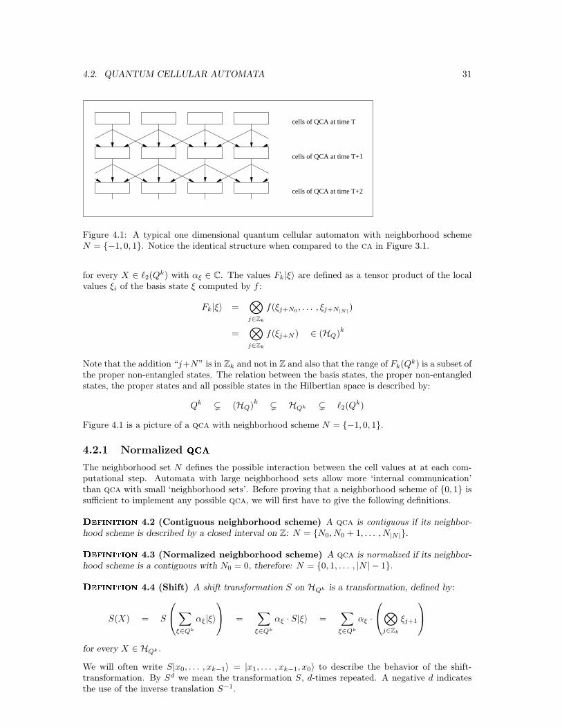
Figure 4.1: A typical one dimensional quantum cellular automaton with neighborhood schemeN = {−1, 0, 1}. Notice the identical structure when compared to the ca in Figure 3.1.
for every X ∈ `2(Qk) with αξ ∈ C. The values Fk|ξ〉 are defined as a tensor product of the local
values ξi of the basis state ξ computed by f :
Fk|ξ〉 =⊗
j∈Zk
f(ξj+N0, . . . , ξj+N|N|
)
=⊗
j∈Zk
f(ξj+N ) ∈ (HQ)k
Note that the addition “j+N” is in Zk and not in Z and also that the range of Fk(Qk) is a subset ofthe proper non-entangled states. The relation between the basis states, the proper non-entangledstates, the proper states and all possible states in the Hilbertian space is described by:
Qk ( (HQ)k ( HQk ( `2(Q
k)
Figure 4.1 is a picture of a qca with neighborhood scheme N = {−1, 0, 1}.
4.2.1 Normalized ���
The neighborhood set N defines the possible interaction between the cell values at at each com-putational step. Automata with large neighborhood sets allow more ‘internal communication’than qca with small ‘neighborhood sets’. Before proving that a neighborhood scheme of {0, 1} issufficient to implement any possible qca, we will first have to give the following definitions.
����������4.2 (Contiguous neighborhood scheme) A qca is contiguous if its neighbor-
hood scheme is described by a closed interval on Z: N = {N0, N0 + 1, . . . , N|N |}.����������
4.3 (Normalized neighborhood scheme) A qca is normalized if its neighbor-hood scheme is a contiguous with N0 = 0, therefore: N = {0, 1, . . . , |N | − 1}.����������
4.4 (Shift) A shift transformation S on HQk is a transformation, defined by:
S(X) = S
∑
ξ∈Qk
αξ|ξ〉
=∑
ξ∈Qk
αξ · S|ξ〉 =∑
ξ∈Qk
αξ ·
⊗
j∈Zk
ξj+1
for every X ∈ HQk .
We will often write S|x0, . . . , xk−1〉 = |x1, . . . , xk−1, x0〉 to describe the behavior of the shift-transformation. By Sd we mean the transformation S, d-times repeated. A negative d indicatesthe use of the inverse translation S−1.
32 CHAPTER 4. QUANTUM CELLULAR AUTOMATA
����������4.5 (Shift equivalence of states) Two configurations X and Y ∈ HQk are shift-
equivalent if there exists a d ∈ Z such that: X = T d(Y ).
Because we allow negative shifts this is an equivalence relation.
����������4.6 (Shift equivalence of automata) Two qca F and F ′ (both with state-set
Q) are shift-equivalent if there exists a d ∈ Z such that for every X ∈ HQk we have: Fk(X) =Sd(F ′
k(X)). A shorthand for this relation is F = Sd ◦ F ′ or F ≡ F ′.
Note that the value d does not depend on the input X or even the size k of the structure. Withthese definitions we can describe the following lemma.
�����4.1 For every qca F there a exists a normalized qca F ′ which is shift-equivalent with
F .Proof. (by construction) Given the qca F = 〈Q,N, f〉 we define F ′ with the tuple 〈Q′, N ′, f ′〉 inthe following way: an equal state set, Q′ = Q, a neighborhood scheme N ′ = {0, 1, . . . , N|N |−N1}and the local function: f ′ : QN ′ → HQ with:
f ′(X0,X1, . . . ,X|N ′|−1) = f(X0,XN2−N1,XN3−N1
, . . . ,X|N ′|−1)
for every X ∈ QN ′
With this construction we have F = SN1 ◦ F ′. 2
This F ′ is called the normalized version of F . If F ′ = Sd◦F we have for every t ∈ N: F t = Sts◦F ′t
(this is because F ◦ S = S ◦ F for every qca F).
4.2.2 Well-formed ���
We start the discussion of well-formed qca with a counter example.
�������
4.1 Take a qca defined by 〈{0, 1}, {0, 1}, f〉, with f defined by:
f(0, 0) = |0〉 f(0, 1) = 12
√2{|0〉 + |1〉
}
f(1, 0) = 12
√2{|0〉 − |1〉} f(1, 1) = |1〉
This gives us the following evolution from the initial state |0, 0, 1〉 ∈ HQ3 :
|0, 0, 1〉 −→F3f(0, 0) ⊗ f(0, 1) ⊗ f(1, 0)
= |0〉0 ⊗{
1
2
√2{|01〉 + |11〉}
}
⊗{
1
2
√2{|0〉2 − |12〉}
}
=1
2{|0, 0, 0〉 − |0, 0, 1〉 + |0, 1, 0〉 − |0, 1, 1〉}
−→F3
1
4{2|0, 0, 0〉 + |0, 0, 1〉 − 3|0, 1, 0〉 + 2|0, 1, 1〉 + |1, 0, 0〉 − 2|1, 1, 0〉 + |1, 1, 1〉}
This last vector is not proper: its norm equals√
22/4 ≈ 1.17. Because this contradicts the lawsof quantum mechanics it is said that this qca is not well-formed: the transformation F3 is notunitary. 3
This shows that our definition of qca allows automata which are not proper. What we mean bywell-formed qca is defined as follows.
����������4.7 (Well-formed
���) A qca F is well-formed if and only if for every k ∈ N+
the corresponding Fk is a unitary transformation.
4.3. PROVING WELL-FORMEDNESS 33
This means that Fk applied to the basis states Qk has to be both norm and angle preserving inthe Hilbertian space `2(Q
k). Because the range of Fk(Qk) consists of proper non-entangled states,it holds for every χ and υ ∈ Qk that Fk|ξ〉 and Fk|υ〉 can be written as a tensor product:
Fk|χ〉 =⊗
i∈Zk
xi and Fk|υ〉 =⊗
i∈Zk
yi
with xi, yi ∈ HQ. The inner-product of these two vectors can therefore be calculated by themultiplication of the inner products of the individual cell-values;
〈Fk|χ〉, Fk|υ〉〉 =
⟨⊗
i∈Zk
xi,⊗
i∈Zk
yi
⟩
=∏
i∈Zk
〈xi, yi〉
For every xi ∈ HQ we know that 〈xi, xi〉 = 1. This means that for every qca the Fk by definitionpreserves the norm of the basis states:
〈Fk|χ〉, Fk|χ〉〉 =
⟨⊗
i∈Zk
xi,⊗
i∈Zk
xi
⟩
=∏
i∈Zk
〈xi, xi〉 = 1
If we want Fk to be angle-preserving we must have for every ξ 6= υ ∈ Qk (and therefore 〈|ξ〉, υ〉 = 0)
〈Fk(χ), Fk(υ)〉 =
⟨⊗
i∈Zk
xi,⊗
i∈Zk
yi
⟩
=∏
i∈Zk
〈xi, yi〉 = 0
This means that there must exist a i ∈ Zk for which 〈xi, yi〉 = 0. The following lemma is easy toprove.
�����4.2 For every qca F , if F ′ is the normalized qca with F = Sd(F ′) (as described in
lemma 4.1) the well-formedness of F equals the well-formedness of F ′.Proof. S is a norm and angle-preserving transformation on HQk . 2
4.3 Proving Well-formedness
In this chapter we will show that the well-formedness restriction can be translated into a localconstraint. This enables us to formulate an algorithm that decides if a given qca is well-formedor not.
����������4.8 (General function of a
���) Given a qca F = 〈Q,N, f〉 we define the gen-
eral function FZ : QZ → (HQ)Z by:
FZ(X) =⊗
i∈Z
f(Xi+N ) ∈ (HQ)Z
for every X ∈ QZ.
This function describes only the first time step of a qca on the two-way infinite basis states. Usinga well-formedness definition for FZ we can investigate the unitarity of the periodic functions Fk
for all values of k.
����������4.9 (Well-formed general function) The function FZ is well-formed if and onlyif for every X 6= Y ∈ QZ there exists an i ∈ Z such that:
〈FZ(X)i, FZ(Y )i〉 = 0
34 CHAPTER 4. QUANTUM CELLULAR AUTOMATA
We will now prove the equivalence of both definitions of well-formedness for qca.
�����4.3 A qca F is well-formed if and only if its corresponding general function FZ is well-
formed.Proof. (If) If F = 〈Q,N, f〉 is not well-formed then there exists a k such that Fk is not angle-preserving. This means that there exists a χ and υ ∈ Qk with χ ⊥ υ and Fk|χ〉 6⊥ Fk|υ〉. If wedefine the two-way infinite states X,Y ∈ QZ by:
X =⊗
i∈Z
χ and Y =⊗
i∈Z
υ
it follows that for every i ∈ Z we have:
FZ(X)i = (Fk|χ〉)imodk and FZ(Y )i = (Fk|υ〉)imodk
Because X 6= Y and FZ(X)i 6⊥ FZ(Y ) for every i ∈ Z, X and Y violate the well-formednessdefinition of FZ.(Only if) Without loss of generality we assume F to be normalized. If FZ is not well-formed thenthere exist two basis states X,Y ∈ QZ with X0 6= Y0 and
〈FZ(X)i, FZ(Y )i〉 6= 0
for every i ∈ Z. In Appendix B it is shown that with the states X and Y we can construct ak ≤ 2|Q|2|N | + |N | and two periodic states X ′, Y ′ ∈ Qk with |X ′〉 ⊥ |Y ′〉 and Fk|X ′〉 6⊥ Fk|Y ′〉.This proves that the qca F is not well-formed. 2
In the above lemma, the proof is more important the conclusion: with little extra effort, we candeduce the following local constraint for well-formed qca. This lemma will be the backbone ofthis thesis.
�����4.4 For every well-formed qca F = 〈Q,N, f〉 there exist two values p, q ∈ Z with:
−|Q|2(N|N|−N1+1) − N1 ≤ p ≤ q < |Q|2(N|N|−N1+1)+ N|N | − 2N1 + 1
such that for every X,Y ∈ QZ with X0 6= Y0 we have:
q∏
i=p
〈FZ(X)i, FZ(Y )i〉 = 0
Proof. Because Lemma 4.3 is ‘if and only if’, it follows (see Appendix B) that for every
normalized, well-formed qca F = 〈Q, {0, . . . , |N | − 1}, f〉 there exists a p ≥ −|Q|2|N |and a
q < |Q|2|N |+ |N |, such that for every X,Y ∈ QZ (with X0 6= Y0), we have:
q∏
i=p
〈FZ(X)i, FZ(Y )i〉 = 0
The constructions in Lemma 4.1 and Lemma 4.2 generalizes this to the desired result. 2
One of the important consequences of this lemma can now be proven directly.
�����4.5 The well-formedness property of a qca F = 〈Q,N, f〉 is decidable.
Proof. If F is not well-formed, there exists a k ∈ N+ such that the finite dimensional transfor-mation Fk is not unitary. Because k is bounded by
k ≤ 2|Q|2(N|N|−N1+1)
this is decidable in finite time. 2
4.3. PROVING WELL-FORMEDNESS 35
The importance of of this bounded restriction lies in the fact that it does not depend on thelocal function f of a qca. For classical reversible ca the range [p, q] is also known as the inverseneighborhood of a ca. Previous work by Jarkko Kari [31] suggests that the bound in Lemma 4.4can be made smaller.
If the domain of a well-formed qca is a proper state-space, the range will also be a properstate-space. In that case we can write Fk : HQk → HQk . If we want to respect the physical laws,only a fraction of the possible qca may be considered meaningful. This resembles the situationwith classical ca where reversibility is a strong restriction on the automata [2, 48] From now onit will be understood that by qca we mean well-formed qca.
4.3.1 A definition of Balancedness
Recently, Christoph Durr et al. [21] raised the question about a definition of ‘balancedness’ in thecase of quantum ca. Here we give a generalization of the classical definition used by Amoroso andPatt [2] (which differs from the one used by Maruoka and Kimura [38]).
����������4.10 (Balanced
���) A qca F = 〈Q, f,N〉 will be called balanced if and only if
∑
x∈QN
| 〈q, f(x)〉 |2 = |Q||N |−1
for every q ∈ HQ,
The following lemma shows the validity of this definition.
�����4.6 Every well-formed qca F = 〈Q, f,N〉 is balanced.
Proof. If we take k = N|N | −N1 + 1, the summation of f(x) is ‘encapsulated’ in the summation
on the set of basis states Qk:
∑
x∈QN
| 〈q, f(x)〉 |2 = |Q||N |−k∑
X∈Qk
| 〈q, (Fk|X〉)0〉 |2
With Lemma 1.1 we can derive the equality:
|Q||N |−k∑
X∈Qk
| 〈q, (Fk|X〉)0〉 |2
= |Q||N |−k∑
X∈Qk
∑
Y ∈Qk−1
| 〈q ⊗ Y, (Fk|X〉)〉 |2
= |Q||N |−k∑
Y ∈Qk−1
∑
X∈Qk
| 〈q ⊗ Y, (Fk|X〉)〉 |2
Because Fk is a unitary transformation such that HFk(Qk) = HQk with q ⊗ Y a vector with norm1 in HQk we reach:
|Q||N |−k∑
y∈Qk−1
∑
X∈Qk
| 〈q ⊗ y, (Fk|X〉)〉 |2
= |Q||N |−k∑
y∈Qk−1
1 = |Q||N |−1
which proves the lemma. 2
This lemma tells us that a qca can only be well-formed if the output values of the local function fare uniformly distributed on the state space HQ. This is not a sufficient restriction for properness,there exist balanced qca which are not well-formed (see Example 4.1).
36 CHAPTER 4. QUANTUM CELLULAR AUTOMATA
4.4 Quiescent Quantum Cellular Automata
In order to relate this thesis to some earlier results about qca, we will give a short description ofqca with quiescent states: Quiescent qca.
����������4.11 (Quiescent���
) A qqca F is a qca defined by the tuple 〈Q,¤, N, f〉, witha quiescent state ¤ ∈ Q, such that f(¤N ) = |¤〉.
This definition is used to overcome the problems of describing the behavior of a qca in an un-countable infinite state space HQZ . The only configurations that are allowed for a qqca arethose with only a finite number of non-quiescent states. Because the left and right tail of such aconfiguration (· · ·¤¤x0x1 · · ·xN¤¤ · · · ) will remain quiescent under the action of a qca, only acountable subset of basis states will be necessary to describe the evolution of the system. The setof basis states of these finite configurations is denoted by Q∗.
For every qqca F the time operator on the superposition of finite configurations F∗ : `2(Q∗) →
`2(Q∗) is defined by
F∗(X) = F∗
∑
ξ∈Q∗
αξ|ξ〉
=∑
ξ∈Q∗
αξ · F∗|ξ〉
for every X ∈ `2(Q∗). The function F∗|ξ〉 on the basis states Q∗ is determined by:
F∗|ξ〉 =∑
j∈Z
f(ξj+N ) (∈ `2(Q∗))
The well-formedness issue of the function F∗ is subtle and has some potential pitfalls. Here is afirst attempt of definition.
����������4.12 (Well-formed
����) Given a qqca F = 〈Q,¤, N, f〉, the function F∗ is
well-formed if and only if for every X,Y ∈ Q∗: the norm of F∗|X〉 equals 1 and X ⊥ Y impliesF∗|X〉 ⊥ F∗|Y 〉.
Because the domain of the local function f is a subset of HQ the norm of F∗(X) will always be 1.The following example will show that there exist well-formed qqca which are not unitary.
�������4.2 Take the qqca F = 〈{¤, •},¤, {0, 1}, f〉, with:
f(¤,¤) = f(•, •) = |¤〉 and f(¤, •) = f(•,¤) = |•〉
The function F∗ is well-formed but not injective and therefore not unitary. This is shown by theequation F∗(X) = |. . . ¤¤ • ¤¤ . . .〉 which can not be satisfied for X ∈ HQ∗ . 3
This example indicates that we have to restrict definition 4.12 to the injective qqca.
����������4.13 (Unitary����
) Given a qqca F = 〈Q,¤, N, f〉, the function F∗ is unitaryif and only if the function F∗ is well-formed and for every Y ∈ Q∗ there exists a X ∈ HQ∗ withF∗(X) = |Y 〉.
Because qqca are a subset of qca as defined in Definition 4.1 we can relate the above definitionof unitary qqca to that of well-formed qca.
�����4.7 If a qqca F = 〈Q,¤, N, f〉 is well-formed as described in Definition 4.7 then the
F∗ is a unitary function.Proof. (by contradiction) If the function F∗ is not unitary there are two possibilities:
4.5. PARTITIONED QUANTUM CELLULAR AUTOMATA 37
1. there exist X ⊥ Y ∈ Q∗ with F∗|X〉 6⊥ F∗|Y 〉2. there exists an X ∈ Q∗ with no predecessor in the domain HQ∗ .
Because X,Y have a left and right tail which is quiescent, it is possible to take k ∈ N+ sufficientlylarge, such that the same possibility holds for Fk. This shows that Fk is not unitary and thereforeproves F not to be well-formed. 2
The converse of this lemma would be: “If a qqca has a unitary F∗, then the qca F is well-formed.”The following example shows that this is not the case.
�������
4.3 Take the qqca F = 〈{¤, 0, 1},¤, {0, 1}, f〉, with f defined by:
f(¤,¤) = |¤〉 f(¤, x) = |¤〉f(x,¤) = |x〉 f(x, y) = |x ⊕ y〉
for every x, y ∈ {0, 1}. Although the function F∗ is unitary, the qca F = 〈{¤, 0, 1}, N, f〉 is notwell-formed. This is shown by F2|0, 0〉 = F2|1, 1〉 = |0, 0〉. 3
We can summarize the above lemma’s and examples in the following hierarchy with F a qqca:
Fk is unitary for every k ∈ N+
FZ is well-formed=⇒6⇐=
F∗ is unitary=⇒6⇐=
F∗ is well-formed
It is still unknown how to define well-formedness for non-quiescent state qca on a two-way infinitestructure with an uncountable dimensional state space HQZ .
4.5 Partitioned Quantum Cellular Automata
The results of the previous sections showed how to decide if a qca is proper or not. What westill do not know is how to construct proper qca with non-trivial behavior. This situation isno different with the problem of non-trivial reversible classical ca. A solution to this problem is(partly) given by partitioned ca [19, 44, 45]. Partitioned ca are constructed in such a way thatthe well-formedness of the automaton is implied by their definition. John Watrous applied thismethod to construct a qca which can simulate a quantum Turing machines [57].
����������4.14 (Partitioned
���) A partitioned quantum cellular automaton (pqca) is
defined by a tuple 〈QL, QC , QR, g〉, with QL, QC and QR finite state sets and g : HQL×QC×QR→
HQL×QC×QRa unitary transformation.
A pqca defines a special type of qca F = 〈Q, {−1, 0, 1}, f〉 with Q = QL×QC×QR. This productstate set reflects the idea to decompose the cell-values into three disjoint parts Left, Center andRight. Each state x ∈ Q is therefore identified by three sub-states: x = xl × xc × xr. This is usedto translate the unitary function g into the local function f : Q3 → HQ by:
f(x−1, x0, x1) = g(xl1 × xc
0 × xr−1)
for every x−1, x0, x1 ∈ Q. Because g is a unitary transformation, the qca F will have a localbehavior which is also unitary. From this it follows that F will be a well-formed qca. See Figure4.2 for an example of such a pqca. With the use of pqca we can define qca in a straightforwardway without having to worry about the well-formedness constraint. This has proven to be a fruitfulconcept in the theory of reversible ca and proper qca. It assures us that the model of qca is anon-trivial way of describing parallel quantum computation.
�����4.8 There exists a proper qca which can simulate a Universal quantum Turing machine
with polynomial time complexity.Proof. See the original paper by John Watrous [57] which combines the earlier results on re-versible ca and quantum Turing Machines. 2
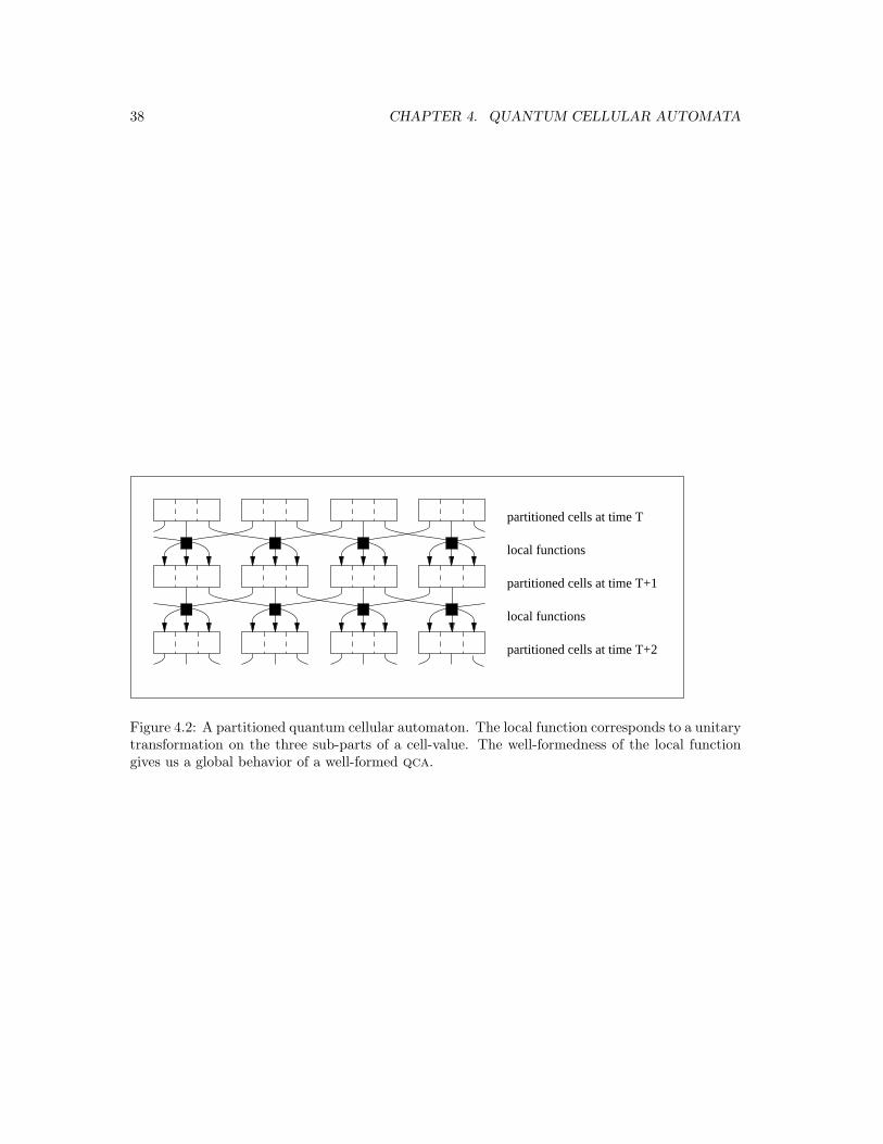
38 CHAPTER 4. QUANTUM CELLULAR AUTOMATA
partitioned cells at time T
partitioned cells at time T+1
partitioned cells at time T+2
local functions
local functions
Figure 4.2: A partitioned quantum cellular automaton. The local function corresponds to a unitarytransformation on the three sub-parts of a cell-value. The well-formedness of the local functiongives us a global behavior of a well-formed qca.
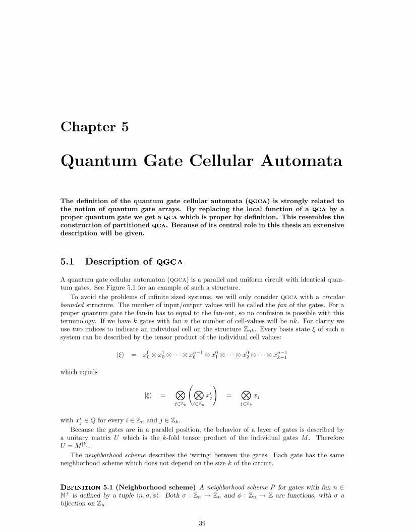
Chapter 5
Quantum Gate Cellular Automata
The definition of the quantum gate cellular automata (����
) is strongly related tothe notion of quantum gate arrays. By replacing the local function of a
���by a
proper quantum gate we get a���
which is proper by definition. This resembles theconstruction of partitioned
���. Because of its central role in this thesis an extensive
description will be given.
5.1 Description of ����
A quantum gate cellular automaton (qgca) is a parallel and uniform circuit with identical quan-tum gates. See Figure 5.1 for an example of such a structure.
To avoid the problems of infinite sized systems, we will only consider qgca with a circularbounded structure. The number of input/output values will be called the fan of the gates. For aproper quantum gate the fan-in has to equal to the fan-out, so no confusion is possible with thisterminology. If we have k gates with fan n the number of cell-values will be nk. For clarity weuse two indices to indicate an individual cell on the structure Znk. Every basis state ξ of such asystem can be described by the tensor product of the individual cell values:
|ξ〉 = x00 ⊗ x1
0 ⊗ · · · ⊗ xn−10 ⊗ x0
1 ⊗ · · · ⊗ x02 ⊗ · · · ⊗ xn−1
k−1
which equals
|ξ〉 =⊗
j∈Zk
(⊗
i∈Zn
xij
)
=⊗
j∈Zk
xj
with xij ∈ Q for every i ∈ Zn and j ∈ Zk.
Because the gates are in a parallel position, the behavior of a layer of gates is described bya unitary matrix U which is the k-fold tensor product of the individual gates M . ThereforeU = M [k].
The neighborhood scheme describes the ‘wiring’ between the gates. Each gate has the sameneighborhood scheme which does not depend on the size k of the circuit.
����������5.1 (Neighborhood scheme) A neighborhood scheme P for gates with fan n ∈N+ is defined by a tuple 〈n, σ, φ〉. Both σ : Zn → Zn and φ : Zn → Z are functions, with σ abijection on Zn.
39
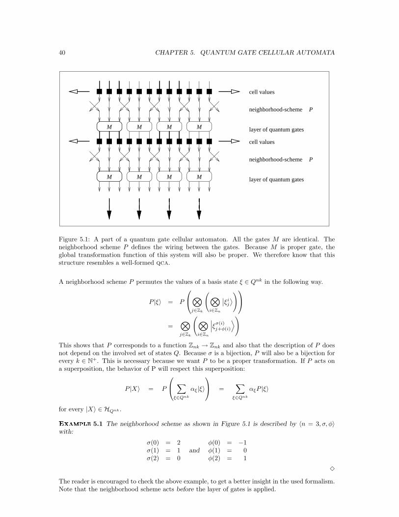
40 CHAPTER 5. QUANTUM GATE CELLULAR AUTOMATA
layer of quantum gates
neighborhood-scheme
layer of quantum gates
neighborhood-scheme
cell values
cell values
M M M M
MMMM
P
P
Figure 5.1: A part of a quantum gate cellular automaton. All the gates M are identical. Theneighborhood scheme P defines the wiring between the gates. Because M is proper gate, theglobal transformation function of this system will also be proper. We therefore know that thisstructure resembles a well-formed qca.
A neighborhood scheme P permutes the values of a basis state ξ ∈ Qnk in the following way.
P |ξ〉 = P
⊗
j∈Zk
(⊗
i∈Zn
∣∣ξi
j
⟩
)
=⊗
j∈Zk
(⊗
i∈Zn
∣∣∣ξ
σ(i)j+φ(i)
⟩)
This shows that P corresponds to a function Znk → Znk and also that the description of P doesnot depend on the involved set of states Q. Because σ is a bijection, P will also be a bijection forevery k ∈ N+. This is necessary because we want P to be a proper transformation. If P acts ona superposition, the behavior of P will respect this superposition:
P |X〉 = P
∑
ξ∈Qnk
αξ|ξ〉
=∑
ξ∈Qnk
αξP |ξ〉
for every |X〉 ∈ HQnk .
�������5.1 The neighborhood scheme as shown in Figure 5.1 is described by 〈n = 3, σ, φ〉with:
σ(0) = 2 φ(0) = −1σ(1) = 1 and φ(1) = 0σ(2) = 0 φ(2) = 1
3
The reader is encouraged to check the above example, to get a better insight in the used formalism.Note that the neighborhood scheme acts before the layer of gates is applied.
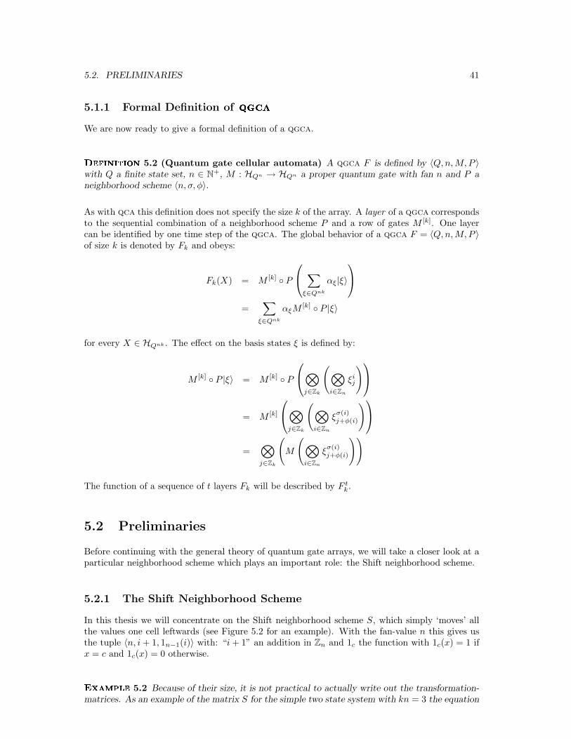
5.2. PRELIMINARIES 41
5.1.1 Formal Definition of ����
We are now ready to give a formal definition of a qgca.
����������5.2 (Quantum gate cellular automata) A qgca F is defined by 〈Q,n,M,P 〉with Q a finite state set, n ∈ N+, M : HQn → HQn a proper quantum gate with fan n and P aneighborhood scheme 〈n, σ, φ〉.
As with qca this definition does not specify the size k of the array. A layer of a qgca correspondsto the sequential combination of a neighborhood scheme P and a row of gates M [k]. One layercan be identified by one time step of the qgca. The global behavior of a qgca F = 〈Q,n,M,P 〉of size k is denoted by Fk and obeys:
Fk(X) = M [k] ◦ P
∑
ξ∈Qnk
αξ|ξ〉
=∑
ξ∈Qnk
αξM[k] ◦ P |ξ〉
for every X ∈ HQnk . The effect on the basis states ξ is defined by:
M [k] ◦ P |ξ〉 = M [k] ◦ P
⊗
j∈Zk
(⊗
i∈Zn
ξij
)
= M [k]
⊗
j∈Zk
(⊗
i∈Zn
ξσ(i)j+φ(i)
)
=⊗
j∈Zk
(
M
(⊗
i∈Zn
ξσ(i)j+φ(i)
))
The function of a sequence of t layers Fk will be described by F tk.
5.2 Preliminaries
Before continuing with the general theory of quantum gate arrays, we will take a closer look at aparticular neighborhood scheme which plays an important role: the Shift neighborhood scheme.
5.2.1 The Shift Neighborhood Scheme
In this thesis we will concentrate on the Shift neighborhood scheme S, which simply ‘moves’ allthe values one cell leftwards (see Figure 5.2 for an example). With the fan-value n this gives usthe tuple 〈n, i + 1, 1n−1(i)〉 with: “i + 1” an addition in Zn and 1c the function with 1c(x) = 1 ifx = c and 1c(x) = 0 otherwise.
�������5.2 Because of their size, it is not practical to actually write out the transformation-matrices. As an example of the matrix S for the simple two state system with kn = 3 the equation
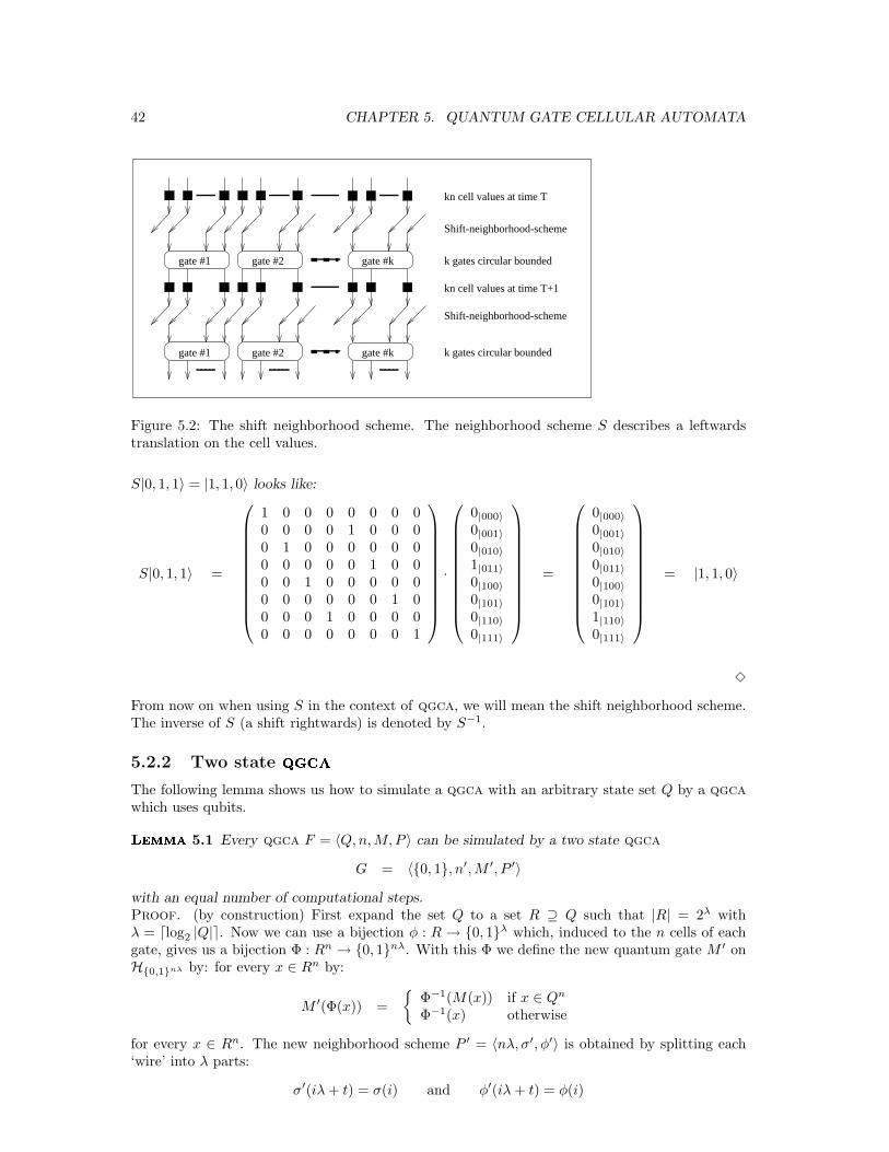
42 CHAPTER 5. QUANTUM GATE CELLULAR AUTOMATA
gate #1 gate #2 gate #k k gates circular bounded
Shift-neighborhood-scheme
kn cell values at time T
kn cell values at time T+1
gate #1 gate #2 gate #k k gates circular bounded
Shift-neighborhood-scheme
Figure 5.2: The shift neighborhood scheme. The neighborhood scheme S describes a leftwardstranslation on the cell values.
S|0, 1, 1〉 = |1, 1, 0〉 looks like:
S|0, 1, 1〉 =
1 0 0 0 0 0 0 00 0 0 0 1 0 0 00 1 0 0 0 0 0 00 0 0 0 0 1 0 00 0 1 0 0 0 0 00 0 0 0 0 0 1 00 0 0 1 0 0 0 00 0 0 0 0 0 0 1
·
0|000〉0|001〉0|010〉1|011〉0|100〉0|101〉0|110〉0|111〉
=
0|000〉0|001〉0|010〉0|011〉0|100〉0|101〉1|110〉0|111〉
= |1, 1, 0〉
3
From now on when using S in the context of qgca, we will mean the shift neighborhood scheme.The inverse of S (a shift rightwards) is denoted by S−1.
5.2.2 Two state ����
The following lemma shows us how to simulate a qgca with an arbitrary state set Q by a qgca
which uses qubits.
�����5.1 Every qgca F = 〈Q,n,M,P 〉 can be simulated by a two state qgca
G = 〈{0, 1}, n′,M ′, P ′〉
with an equal number of computational steps.Proof. (by construction) First expand the set Q to a set R ⊇ Q such that |R| = 2λ withλ = dlog2 |Q|e. Now we can use a bijection φ : R → {0, 1}λ which, induced to the n cells of eachgate, gives us a bijection Φ : Rn → {0, 1}nλ. With this Φ we define the new quantum gate M ′ onH{0,1}nλ by: for every x ∈ Rn by:
M ′(Φ(x)) =
{Φ−1(M(x)) if x ∈ Qn
Φ−1(x) otherwise
for every x ∈ Rn. The new neighborhood scheme P ′ = 〈nλ, σ′, φ′〉 is obtained by splitting each‘wire’ into λ parts:
σ′(iλ + t) = σ(i) and φ′(iλ + t) = φ(i)
5.3. EVERY QGCA DESCRIBES A QCA 43
for every i ∈ Zn and t ∈ Zλ.
This qgca G = 〈{0, 1}, nλ,M ′, 〈nλ, σ′, φ′〉〉 simulates the original qgca according to thebijection φ. If an illegal state is encoded (x /∈ Qn) the M ′-gate behaves like the identity. Thisshows that M ′ is a proper transformation. 2
5.2.3 Combining neighborhood schemes
Here we will show how to express a neighborhood scheme R ◦ P which is a combination of twoinitial schemes P and R. Given the two neighborhood schemes P = 〈n, σ, φ〉 and R = 〈n, ς, ϕ〉, wecan define the action of P by:
P
⊗
j∈Zk
(⊗
i∈Zn
xij
)
=⊗
j∈Zk
(⊗
i∈Zn
xσ(i)j+φ(i)
)
=⊗
j∈Zk
(⊗
i∈Zn
yij
)
If we use the y expressions to describe the effect of R4 we get:
R
⊗
j∈Zk
(⊗
i∈Zn
yij
)
=⊗
j∈Zk
(⊗
i∈Zn
yς(i)j+ϕ(i)
)
The combination of R and P therefore obeys (using the equation yij = x
σ(i)j+φ(i)):
R ◦ P
⊗
j∈Zk
(⊗
i∈Zn
xij
)
=⊗
j∈Zk
(⊗
i∈Zn
xσ(ς(i))j+ϕ(i)+φ(ς(i))
)
This shows us that we can write:
R ◦ P = 〈n, ς(i), ϕ(i)〉 ◦ 〈n, σ(i), φ(i)〉 = 〈n, σ ◦ ς(i), ϕ(i) + φ ◦ ς(i)〉
With regard to the shift neighborhood scheme we have: S = 〈n, i + 1, 1n−1(i)〉 and
Sn ◦ P = 〈n, i, 1〉 ◦ 〈n, σ(i), φ(i)〉 = 〈n, σ(i), 1 + φ(i)〉 = P ◦ Sn
5.3 Every ����describes a ���
If we look at the figures 4.2 and 5.1 we see a great resemblance. We already know that pqca area special kind of qca. We will now prove the same holds for qgca.
�����5.2 Every proper qgca F = 〈Q,n,M,P 〉 defines a well-formed qca qca F = 〈Qn, N, f〉.
Proof. The correspondence between the values of the qgca and those of the qca is expressedby:
xj = x0j ⊗ · · · ⊗ xn−1
j
for every xj ∈ Qn. The neighborhood scheme P = 〈n, σ, φ〉 gives us the neighborhood set of F
according to: N = {φ(i) | i ∈ Zn}. The local function f : (Qn)N → HQn now obeys:
f(xN ) = M
(⊗
i∈Zn
xσ(i)φ(i)
)
44 CHAPTER 5. QUANTUM GATE CELLULAR AUTOMATA
By this construction, for every k ∈ N+ it holds that:
Gk
⊗
j∈Zk
(⊗
i∈Zn
xij
)
= M [k] · Pk
⊗
j∈Zk
(⊗
i∈Zn
xij
)
= M [k]
⊗
j∈Zk
(⊗
i∈Zn
xσ(i)j+φ(i)
)
=⊗
j∈Zk
(
M
(⊗
i∈Zn
xσ(i)j+φ(i)
))
=⊗
j∈Zk
f(xj+N )
= Fk
⊗
j∈Zk
xj
2
As with pqca the well-formedness of a qgca 〈Q,n,M,P 〉 is certified by the well-formedness ofthe gate and the neighborhood scheme.
Chapter 6
���, �
���, and
����are
Equivalent
In this chapter will prove the equivalence of all three models for quantum cellularautomata. By ‘equivalence’ we mean that every
���can be simulated by a
����,
every����
by a ����
, every ����
by a���
etc. All these simulations have atmost linear slowdown. Our main problem is to prove that every proper
���can be
simulated by a����
.
6.1 A Definition of Equivalence
Suppose we have two qca F and G. If we say that G simulates F , we mean that there are two‘simple transformations’ Φt and Ψt such that Φt ◦Gλt ◦Ψt equals F t. The Gλ-expression indicatesa simulation with only linear (proportional to λ) slowdown. The transformations must be ‘simple’because we want G to do the actual calculation. Or in the words of Marvin Minsky[43]:
( . . . ) for if one is permitted an arbitrary partial-recursive computation to do theencoding ( . . . ), then one could use as the code the result of the Turing-machinecomputation itself, and this would surely be considered a cheat!
With this warning in mind we pose the following (inductive) definition:
����������6.1 (Simple transformation) Let P,Q,R be state sets and a, b, c, d ∈ N+. Sim-
ple transformations depending on t ∈ Z, are constructed by the following three procedures:
1. If φ : P a → Qb is a total function, then Φ(t) : P aZ → QbZ defined by:
Φ(t)
(⊗
i∈Z
xi
)
=⊗
i∈Z
[φ(xil, . . . , xil+l−1)]im:(im+m−1)
is a simple transformation.
2. If Φ(t) is a simple transformation, then the transformations S ◦ Φ(t), S−1 ◦ Φ(t), St ◦ Φ(t)and S−t ◦ Φ(t) are also simple (with S the shift translation).
3. If Φ(t) : P aZ → QbZ and Ψ(t) : QcZ → RdZ are simple transformations, then the combinationΘ(t) : P acZ → Rbd described by Θ(t) = Ψ(t) ◦ Φ(t) is also a simple transformation.
A simple transformation Φ(t) : P aZ → QbZ defines for every k ∈ N+ the simple transformationΦk(t) : HP ka → HQkb which obeys the superposition principle of the state space.
Now we can formulate the definition for simulation of quantum cellular automata.
45
46 CHAPTER 6. QCA, PQCA, AND QGCA ARE EQUIVALENT
����������6.2 (Simulating
���) A qca G = 〈P,N ′, g〉 can simulates a qca F = 〈Q,N, f〉,
if there exists a tuple 〈λ,Φ,Ψ〉 with Φ(t) : QaZ → P bZ and Ψ(t) : P bZ → QaZ simple transforma-tions and λ ∈ N such that for every t, k ∈ N+ and X ∈ HQka we have:
F tka(X) = Φka(t) ◦ Gλt
kb ◦ Ψkb(t)(X)
Or in other words:
F tka = Φka(t) ◦ (Gkb)
λt ◦ Ψkb(t)
If no misunderstanding is possible we can shorten this to: F t = Φt ◦ Gλt ◦ Ψt.
When F can be simulated by G, we will write “{F} ¹ {G}”. This relation is certified by 〈λ,Φ,Ψ〉,this tuple will also be called the encoding of F into G.
With this definition we can define the notion of equivalence for quantum cellular automata.
����������6.3 (Equivalent
���) Two qca F and G will be called equivalent if and only if
F can simulate G and G can simulate F .
Consequently we will denote this by “{F} ' {G}”. For every qca F , G and H we now have:
1. {F} ¹ {F}
2. If {F} ¹ {G} and {G} ¹ {H}, then {F} ¹ {H}
3. If {F} ¹ {G} and {G} ¹ {F}, then {F} ' {G}
If we take the ‘identity-encoding’ 〈1, I, I〉, we see that 1 holds, whereas 3 holds by definition. Thesecond rule needs more explanation.
If {F} ¹ {G} is certified by 〈λ,Φ,Ψ〉 and {G} ¹ {H} by 〈µ,∆,Λ〉, we have (in shorthand):F t = Φt ◦ Gλt ◦ Ψt and Gj = ∆j ◦ Hµj ◦ Λj and therefore:
F t = Φt ◦ ∆λt ◦ Hµλt ◦ Λλt ◦ Ψt
By defining Ξt = Φt ◦ ∆λt and Υt = Λλt ◦ Ψt, we see by Definition 6.1 that Ξ and Υ are simpletransformations. This shows that 〈µλ,Ξ,Υ〉 certifies the {F} ¹ {H}-relation.
Because the relations “¹” and “'” are defined on sets of qca we can extend their domain inthe following way:
����������6.4 (Simulating sets of���
) If A and B are sets of quantum cellular automata,we say that B can simulate A if and only if for every F ∈ A there exists a G ∈ B which simulatesF . This will be denoted by “A ¹ B”.
����������6.5 (Equivalent sets of
���) If A and B are sets of quantum cellular automata,
we that A and B are equivalent if and only if both A ¹ B and B ¹ A holds. This equivalence isdenoted by A ' B.
With this definition we have for every set of quantum cellular automata A,B and C:
1. A ¹ A
2. If A ¹ B and B ¹ C, then A ¹ C
3. If A ¹ B and B ¹ A, then A ' B
4. A ' A
5. If A ' B, then B ' A
6. If A ' B and “B ' C”, then A ' C
6.2. SOME PRELIMINARY RESULTS 47
These rules show that ¹ is a partial ordering and ' is a equivalence relation. A few concludingremarks about the above definitions:
• A ' B does not necessarily mean that for every F ∈ A there exists a G ∈ B, with F and Gequivalent.
• The constant “λ” indicates the linear slowdown of the simulation.
• If A ⊆ B then automatically A ¹ B.
• If F is shift equivalent with G then F and G are also equivalent.
• An interesting question is whether the ¹-relation is total or not. Does for every qca F andG it holds that {F} ¹ {G} or {G} ¹ {F}?
6.2 Some Preliminary Results
The strategy of this chapter is to reduce the different sets of qca, pqca and qgca to each otherin a step-by-step way. Let us first summarize the relations we already know. We begin by usingthe fact that qgca and pqca are subsets of qca.
�����6.1 pqca ¹ qca.
Proof. Partitioned qca are just a special type of qca, therefore pqca ⊆ qca. 2
�����6.2 qgca ¹ qca.
Proof. Lemma 5.2 proves qgca ⊆ qca. 2
To reduce the class of qca we use the following lemma.
�����6.3 The subset of normalized qca is equivalent with the general set of qca.
Proof. Normalized qca are a subset of qca. Lemma 4.1 proves that every qca is shift-equivalentwith a normalized qca, thus qca ' qcanormalized. 2
Now we will prove a new result which will simplify our reasoning about simulating qca consider-ably.
�����6.4 The set of qca with neighborhood set N = {0, 1} is equivalent with the set of
normalized qca.Proof.(by construction) For every normalized qca F defined by 〈Q, {0, . . . , |N | − 1}, f〉 thereexists a qca G with neighborhood set NG = {0, 1} which simulates F with no slowdown. Inorder to get a neighborhood size 2 we expand the set of states: G is described by the tuple〈Qr−1, {0, 1}, g〉. The local function g : (Q|N |−1)2 → HQ|N|−1 in this definition obeys
g(x1:(|N |−1), x|N |:(2|N |−2)
)= f(x1:|N |) ⊗ f(x2:(|N |+1)) ⊗ · · · ⊗ f(x(|N |−1):(2|N |−2))
with xi ∈ Q and therefore xa:(a+|N |−2) ∈ Q|N |−1.The encoding of F into G is established by the simple transformations:
Ψ : (Q)|N |−1 → (Q|N |−1) with Ψ(x1:|N |−1) = x1 ⊗ · · · ⊗ x|N |−1
Φ : (Q|N |−1) → (Q)|N |−1 with Φ(x1 ⊗ · · · ⊗ x|N |−1) = x1:|N |−1
The tuple 〈1,Φ,Ψ〉 now certifies {F} ¹ {G} with NG = {0, 1}. 2
A simple extension of this lemma will be the last of our preliminary results.
�����6.5 The set of qca with neighborhood N = {0, 1} is equivalent with the set of qca.
Proof. Combine the results: qca ' qcanormalized and qcanormalized ' qcaN={0,1} 2
48 CHAPTER 6. QCA, PQCA, AND QGCA ARE EQUIVALENT
6.3 Shift Neighborhood Scheme is Universal
In this section we will prove that every neighborhood scheme can be simulated using the shift-scheme S. It will be understood that k is the number of gates, n is the fan of the gates, P and Rare neighborhood schemes and M1,M2, . . . are proper quantum gates.
6.3.1 Periodic ����
A periodic qgca is a non-homogeneous qgca. It is build by a periodic pattern of different gatesand neighborhood schemes.
����������6.6 (Periodic����
) A periodic qgca F of µ layers is defined by a tuple
F = 〈Q,n, µ,M0, . . . ,Mµ−1, P0, . . . , Pµ−1〉
with Mi proper quantum gates and Pi proper neighborhood schemes for 0 ≤ i < µ. The unitaryoperator of the first µ layers of this qca is defined by:
Fk =
0∏
i=µ−1
(
(Mi)[k] · Pi
)
(Notice the order of the index i and the fact that Fk is defined as the operator of several layers.)
�������
6.1 With the 3-periodic qgca F = 〈Q,n, 3, A0, A1, A2, P0, P1, P2〉; the behavior ofthe first 3j layers is described by:
F jk =
(
A[k]2 · P2 · A[k]
1 · P1 · A[k]0 · P0
)j
3
A periodic qgca with µ layers will be call a µ-periodic qgca. An 1-periodic qgca is again aregular qgca. This definition is a side-step from the regular classes qca, pqca, and qgca toallow a more flexible way of defining quantum cellular automata. After that it will be proven thatevery periodic qgca corresponds to a qgca.
6.3.2 Simulating Neighborhood Schemes
By allowing different layers in a qgca we can construct a periodic qgca that mimics the behaviorof a neighborhood scheme. This is shown in the following lemma.
�����6.6 For every qgca F = 〈Q,n,M,P 〉 there exists a periodic qgca G defined by
G = 〈Q,n, µ,M0, . . . ,Mµ−1, S, . . . , S〉
which is shift equivalent with F .Proof. See Appendix C for a proof by construction of this lemma. 2
Figure 6.1 shows us an example of such a simulation by a periodic qgca.
�������6.2 The qgca F = 〈Q, 3,M, P 〉 with a neighborhood scheme P = 〈3, σ, φ〉 and
σ(0) = 2 φ(0) = −1
σ(1) = 1 φ(1) = 1
σ(2) = 0 φ(2) = 0
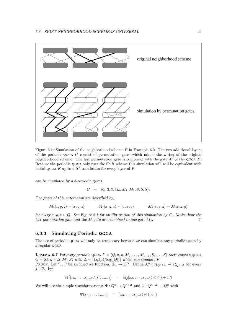
6.3. SHIFT NEIGHBORHOOD SCHEME IS UNIVERSAL 49
original neighborhood scheme
simulation by permutation gates
Figure 6.1: Simulation of the neighborhood scheme P in Example 6.2. The two additional layersof the periodic qgca G consist of permutation gates which mimic the wiring of the originalneighborhood scheme. The last permutation gate is combined with the gate M of the qgca F .Because the periodic qgca only uses the Shift scheme this simulation will will be equivalent withinitial qgca F up to a S3 translation for every layer of F .
can be simulated by a 3-periodic qgca
G = 〈Q, 3, 3,M0,M1,M2, S, S, S〉.
The gates of this automaton are described by:
M0|x, y, z〉 = |x, y, z〉 M1|x, y, z〉 = |z, x, y〉 M2|x, y, z〉 = M |x, z, y〉
for every x, y, z ∈ Q. See Figure 6.1 for an illustration of this simulation by G. Notice how thelast permutation gate and the M gate are combined to one gate M2. 3
6.3.3 Simulating Periodic ����
The use of periodic qgca will only be temporary because we can simulate any periodic qgca bya regular qgca.
�����6.7 For every periodic qgca F = 〈Q,n, µ,M0, . . . ,Mµ−1, S, . . . , S〉 there exists a qgca
G = 〈Q,n + ∆,M ′, S〉 with ∆ = dlog(µ)/log(|Q|)e which can simulate F .Proof. Let p. . .q be an injective function: Zµ → Q∆. Define M ′ : HQn+∆ → HQn+∆ for everyj ∈ Zµ by:
M ′|x0, . . . , xn−2; pjq;xn−1〉 = Mj |x0, . . . , xn−1〉 ⊗ |pj + 1q〉
We will use the simple transformations: Ψ : Qn → Qn+∆ and Φ : Qn+∆ → Qn with
Ψ(x0, . . . , xn−1) = (x0, . . . , xn−1) ⊗ (p0q)
50 CHAPTER 6. QCA, PQCA, AND QGCA ARE EQUIVALENT
and
Φ(x0, . . . , xn−1, x′1, . . . , x′
∆) = (x0, . . . , xn−1)
Now 〈λ = µ,Φ,Ψ〉 certifies the {F} ¹ {G} relation according to:
Φk(n+∆) ◦ Gλtk(n+∆) ◦ Ψkn = F t
kn
2
An example will show us how this procedure can be applied to a small periodic qgca.
�������
6.3 If a 2-periodic qgca F = 〈{0, 1}, 3, 2,M0,M1, S, S〉 has the following behaviorfor the circuit size k = 2:
F2(X) = M[2]1 · S · M [2]
0 · S|x00, x
10, x
20, x
01, x
11, x
21〉
= M[2]1 · S · M [2]
0 |x10, x
20, x
01, x
11, x
21, x
00〉
= M[2]1 · S
(M0|x1
0, x20, x
01〉 ⊗ M0|x1
1, x21, x
00〉
)
= M[2]1 · S
(|y0
0 , y10 , y2
0 , y01 , y1
1 , y21〉
)
= M[2]1
(|y1
0 , y20 , y0
1 , y11 , y2
1 , y00〉
)
= M1|y10 , y2
0 , y01〉 ⊗ M1|y1
1 , y21 , y0
0〉= |z0
0 , z10 , z2
0 , z01 , z1
1 , z21〉
= (Z)
Then, with
Ψ(x00, x
10, x
20) = (x0
0, x10, x
20; p0q) and Φ(x0
0, x10, x
20;x
′0) = (x0
0, x10, x
20)
the tuple 〈λ = 2,Φ,Ψ〉 certifies the simulation of F by G = 〈{0, 1}, 4,M ′, S〉 as is illustrated by:
Φ8 ◦(
M ′[2] · S)2
◦ Ψ6(X) = Φ8 ◦ M ′[2] · S · M ′[2] · S|x00, x
10, x
20, p0q, x0
1, x11, x
21, p0q〉
= Φ8 ◦ M ′[2] · S · M ′[2]|x10, x
20, p0q, x0
1, x11, x
21, p0q, x0
0〉= Φ8 ◦ M ′[2] · S
(M ′|x1
0, x20, p0q, x0
1〉 ⊗ M ′|x11, x
21, p0q, x0
0〉)
= Φ8 ◦ M ′[2] · S(M0|x1
0, x20, x
01〉 ⊗ |p1q〉 ⊗ M0|x1
1, x21, x
00〉 ⊗ |p1q〉
)
= Φ8 ◦ M ′[2] · S|y00 , y1
0 , y20 , p1q, y0
1 , y11 , y2
1 , p1q〉= Φ8 ◦ M ′[2]|y1
0 , y20 , p1q, y0
1 , y11 , y2
1 , p1q, y00〉
= Φ8 ◦ M ′|y10 , y2
0 , p1q, y01〉 ⊗ M ′|y1
1 , y21 , p1q, y0
0〉= Φ8 ◦ M1|y1
0 , y20 , y0
1〉 ⊗ |p0q〉 ⊗ M1|y11 , y2
1 , y00〉 ⊗ |p0q〉
= Φ8|z00 , z1
0 , z20 , p0q, z0
1 , z11 , z2
1 , p0q〉= |z0
0 , z10 , z2
0 , z01 , z1
1 , z21〉
= (Z)
3
With the use of above lemmas we can now state the following theorem about the simulation ofperiodic qgca.
�������6.1 Every periodic qgca F = 〈Q,n, µ,M0, . . . ,Mµ−1, P0, . . . , Pµ−1〉 can be simu-
lated by a regular qgca G = 〈Q,n′,M ′, S〉 with only linear slowdown. This can be abridged bythe statement: qgcaperiodic ' qgcaS.
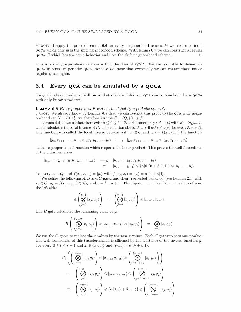
6.4. EVERY QCA CAN BE SIMULATED BY A QGCA 51
Proof. If apply the proof of lemma 6.6 for every neighborhood scheme Pi we have a periodicqgca which only uses the shift neighborhood scheme. With lemma 6.7 we can construct a regularqgca G which has the same behavior and uses the shift neighborhood scheme. 2
This is a strong equivalence relation within the class of qgca. We are now able to define ourqgca in terms of periodic qgca because we know that eventually we can change those into aregular qgca again.
6.4 Every ���can be simulated by a ����
Using the above results we will prove that every well-formed qca can be simulated by a qgca
with only linear slowdown.
�����6.8 Every proper qca F can be simulated by a periodic qgca G.
Proof. We already know by Lemma 6.5 that we can restrict this proof to the qca with neigh-borhood set N = {0, 1}, we therefore assume F = 〈Q, {0, 1}, f〉.
Lemma 4.4 shows us that there exist a ≤ 0 ≤ b ∈ Z and a function g : R → Q with R ⊂ HQb−a+1
which calculates the local inverse of F . This function obeys: ξ ⊥ χ if g(ξ) 6= g(χ) for every ξ, χ ∈ R.The function g is called the local inverse because with xi ∈ Q and |yi〉 = f(xi, xi+1) the function
|ya, ya+1, . . . , y−1, x0, y0, y1, . . . , yb〉 ←−g |ya, ya+1, . . . , y−1, y0, y0, y1, . . . , yb〉
defines a proper transformation which respects the inner product. This proves the well-formednessof the transformation
|ya, . . . , y−1, x0, y0, y1, . . . , yb〉 −→f0|ya, . . . , y0, y0, y1, . . . , yb〉
≡ |ya, . . . , y−1〉 ⊗ {α|0, 0〉 + β|1, 1〉} ⊗ |y1, . . . , yb〉
for every xi ∈ Q, and f(xi, xi+1) = |yi〉 with f(x0, x1) = |y0〉 = α|0〉 + β|1〉.We define the following A,B and C gates and their ‘requested behavior’ (see Lemma 2.1) with
xj ∈ Q; yj = f(xj , xj+1) ∈ HQ and r = b − a + 1. The A-gate calculates the r − 1 values of y onthe left-side:
A
r−1⊗
j=0
|xj , xj〉
=
r−2⊗
j=0
|xj , yj〉
⊗ |xr−1, xr−1〉
The B-gate calculates the remaining value of y:
B
r−2⊗
j=1
|xj , yj〉
⊗ |xr−1, xr−1〉 ⊗ |xr, yr〉
=r⊗
j=1
|xj , yj〉
We use the C-gates to replace the x values by the new y values. Each C gate replaces one x value.The well-formedness of this transformation is affirmed by the existence of the inverse function g.For every 0 ≤ t ≤ r − 1 and zi ∈ {xi, yi} and |yt−a〉 = α|0〉 + β|1〉:
Ct
t−a−1⊗
j=t
|zj , yj〉
⊗ |xt−a, yt−a〉 ⊗
t+r−1⊗
j=t−a+1
|zj , yj〉
=
t−a−1⊗
j=t
|zj , yj〉
⊗ |yt−a, yt−a〉 ⊗
t+r−1⊗
j=t−a+1
|zj , yj〉
≡
t−a−1⊗
j=t
|zj , yj〉
⊗ {α|0, 0〉 + β|1, 1〉} ⊗
t+r−1⊗
j=t−a+1
|zj , yj〉
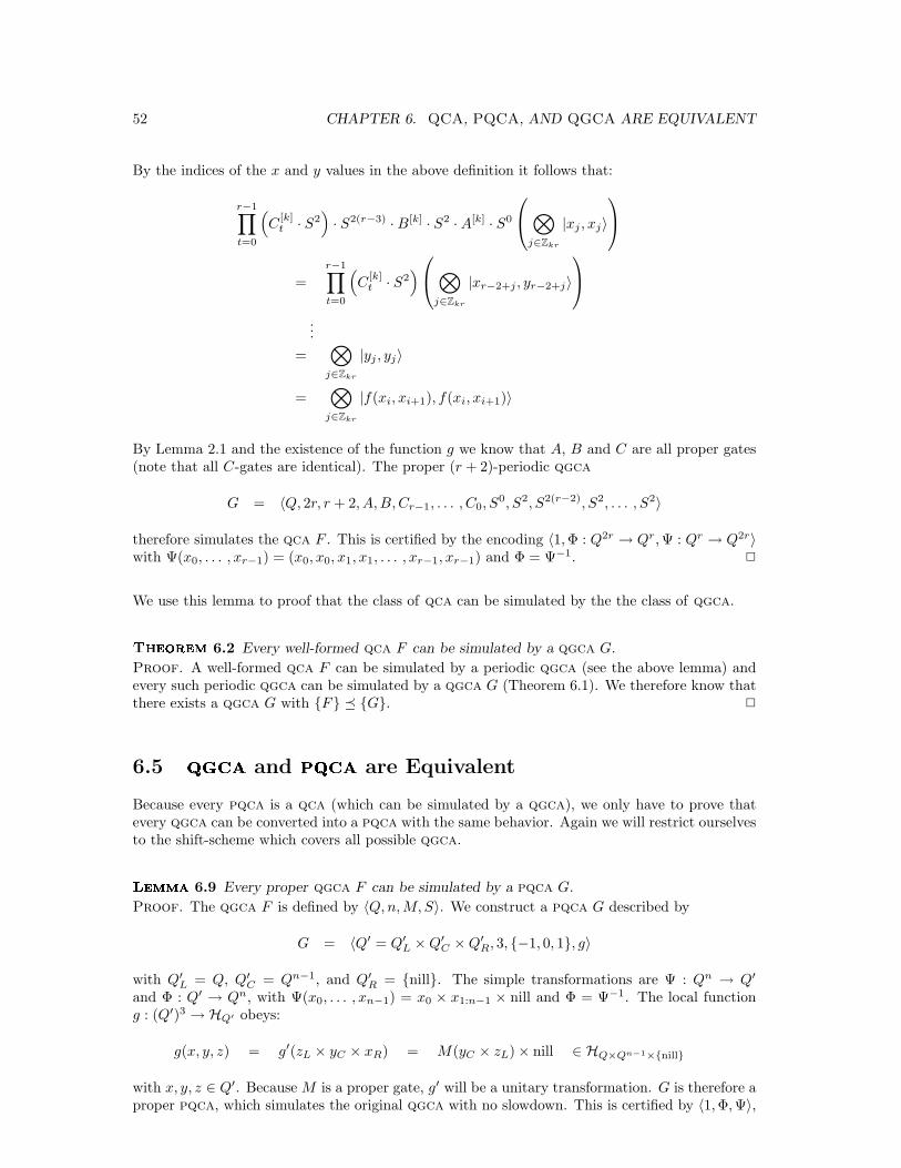
52 CHAPTER 6. QCA, PQCA, AND QGCA ARE EQUIVALENT
By the indices of the x and y values in the above definition it follows that:
r−1∏
t=0
(
C[k]t · S2
)
· S2(r−3) · B[k] · S2 · A[k] · S0
⊗
j∈Zkr
|xj , xj〉
=r−1∏
t=0
(
C[k]t · S2
)
⊗
j∈Zkr
|xr−2+j , yr−2+j〉
...
=⊗
j∈Zkr
|yj , yj〉
=⊗
j∈Zkr
|f(xi, xi+1), f(xi, xi+1)〉
By Lemma 2.1 and the existence of the function g we know that A, B and C are all proper gates(note that all C-gates are identical). The proper (r + 2)-periodic qgca
G = 〈Q, 2r, r + 2, A,B,Cr−1, . . . , C0, S0, S2, S2(r−2), S2, . . . , S2〉
therefore simulates the qca F . This is certified by the encoding 〈1,Φ : Q2r → Qr,Ψ : Qr → Q2r〉with Ψ(x0, . . . , xr−1) = (x0, x0, x1, x1, . . . , xr−1, xr−1) and Φ = Ψ−1. 2
We use this lemma to proof that the class of qca can be simulated by the the class of qgca.
�������6.2 Every well-formed qca F can be simulated by a qgca G.
Proof. A well-formed qca F can be simulated by a periodic qgca (see the above lemma) andevery such periodic qgca can be simulated by a qgca G (Theorem 6.1). We therefore know thatthere exists a qgca G with {F} ¹ {G}. 2
6.5 ����and ����are Equivalent
Because every pqca is a qca (which can be simulated by a qgca), we only have to prove thatevery qgca can be converted into a pqca with the same behavior. Again we will restrict ourselvesto the shift-scheme which covers all possible qgca.
�����6.9 Every proper qgca F can be simulated by a pqca G.
Proof. The qgca F is defined by 〈Q,n,M, S〉. We construct a pqca G described by
G = 〈Q′ = Q′L × Q′
C × Q′R, 3, {−1, 0, 1}, g〉
with Q′L = Q, Q′
C = Qn−1, and Q′R = {nill}. The simple transformations are Ψ : Qn → Q′
and Φ : Q′ → Qn, with Ψ(x0, . . . , xn−1) = x0 × x1:n−1 × nill and Φ = Ψ−1. The local functiong : (Q′)3 → HQ′ obeys:
g(x, y, z) = g′(zL × yC × xR) = M(yC × zL) × nill ∈ HQ×Qn−1×{nill}
with x, y, z ∈ Q′. Because M is a proper gate, g′ will be a unitary transformation. G is therefore aproper pqca, which simulates the original qgca with no slowdown. This is certified by 〈1,Φ,Ψ〉,
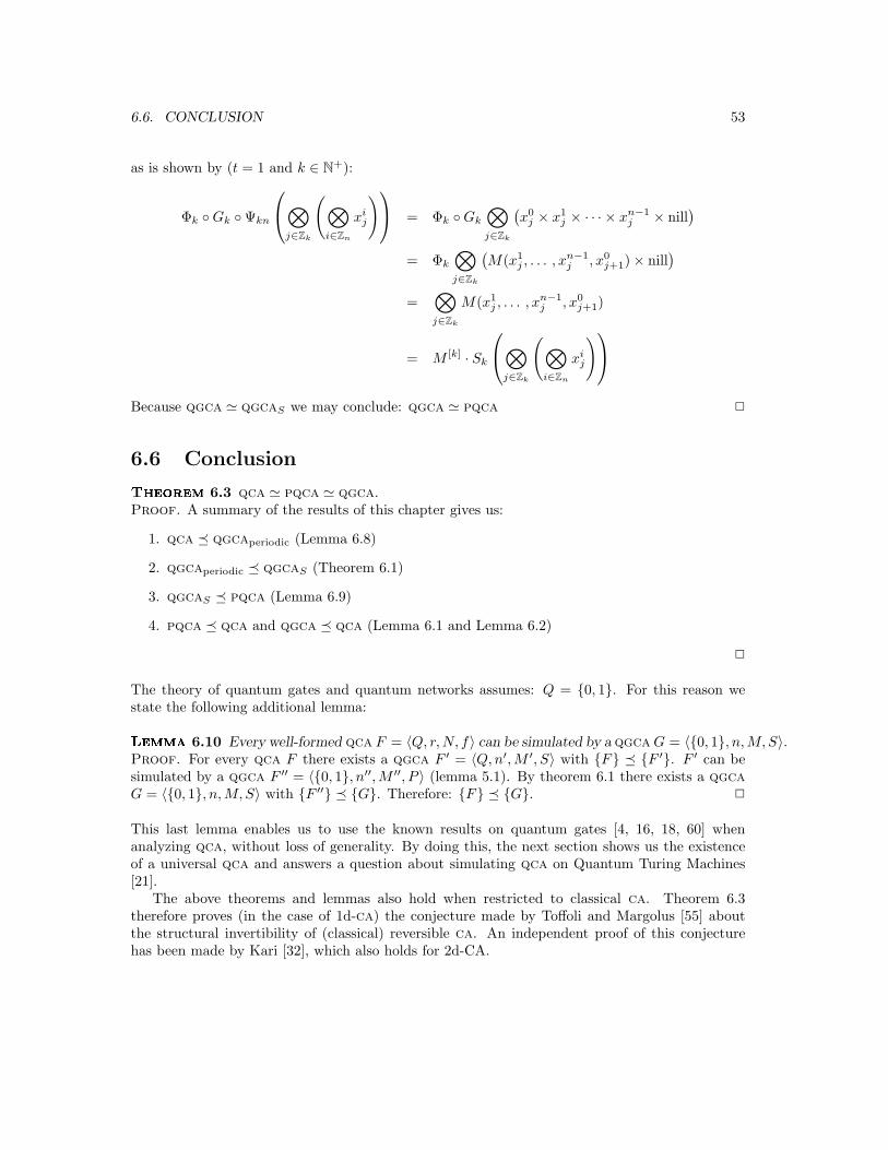
6.6. CONCLUSION 53
as is shown by (t = 1 and k ∈ N+):
Φk ◦ Gk ◦ Ψkn
⊗
j∈Zk
(⊗
i∈Zn
xij
)
= Φk ◦ Gk
⊗
j∈Zk
(x0
j × x1j × · · · × xn−1
j × nill)
= Φk
⊗
j∈Zk
(M(x1
j , . . . , xn−1j , x0
j+1) × nill)
=⊗
j∈Zk
M(x1j , . . . , xn−1
j , x0j+1)
= M [k] · Sk
⊗
j∈Zk
(⊗
i∈Zn
xij
)
Because qgca ' qgcaS we may conclude: qgca ' pqca 2
6.6 Conclusion�������
6.3 qca ' pqca ' qgca.Proof. A summary of the results of this chapter gives us:
1. qca ¹ qgcaperiodic (Lemma 6.8)
2. qgcaperiodic ¹ qgcaS (Theorem 6.1)
3. qgcaS ¹ pqca (Lemma 6.9)
4. pqca ¹ qca and qgca ¹ qca (Lemma 6.1 and Lemma 6.2)
2
The theory of quantum gates and quantum networks assumes: Q = {0, 1}. For this reason westate the following additional lemma:
�����6.10 Every well-formed qca F = 〈Q, r,N, f〉 can be simulated by a qgca G = 〈{0, 1}, n,M, S〉.
Proof. For every qca F there exists a qgca F ′ = 〈Q,n′,M ′, S〉 with {F} ¹ {F ′}. F ′ can besimulated by a qgca F ′′ = 〈{0, 1}, n′′,M ′′, P 〉 (lemma 5.1). By theorem 6.1 there exists a qgca
G = 〈{0, 1}, n,M, S〉 with {F ′′} ¹ {G}. Therefore: {F} ¹ {G}. 2
This last lemma enables us to use the known results on quantum gates [4, 16, 18, 60] whenanalyzing qca, without loss of generality. By doing this, the next section shows us the existenceof a universal qca and answers a question about simulating qca on Quantum Turing Machines[21].
The above theorems and lemmas also hold when restricted to classical ca. Theorem 6.3therefore proves (in the case of 1d-ca) the conjecture made by Toffoli and Margolus [55] aboutthe structural invertibility of (classical) reversible ca. An independent proof of this conjecturehas been made by Kari [32], which also holds for 2d-CA.
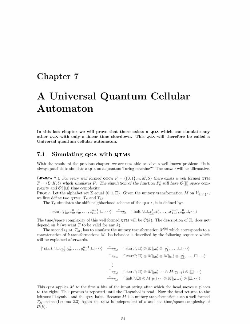
Chapter 7
A Universal Quantum Cellular
Automaton
In this last chapter we will prove that there exists a���
which can simulate anyother
���with only a linear time slowdown. This
���will therefore be called a
Universal quantum cellular automaton.
7.1 Simulating ���with ���s
With the results of the previous chapter, we are now able to solve a well-known problem: “Is italways possible to simulate a qca on a quantum Turing machine?” The answer will be affirmative.
�����7.1 For every well formed qgca F = 〈{0, 1}, n,M, S〉 there exists a well formed qtm
T = 〈Σ,K, δ〉 which simulates F . The simulation of the function F tk will have O(‖) space com-
plexity and O(‖t) time complexity.Proof. Let the alphabet set Σ equal {0, 1,¤}. Given the unitary transformation M on H{0,1}n ,we first define two qtms: TS and TM .
The TS simulates the shift neighborhood scheme of the qgca, it is defined by:
|pstartq;¤, x00, x
10, . . . , xn−1
k−1 ,¤, · · ·〉 ∗−→TS|phaltq;¤, x1
0, x20, . . . , xn−1
k−1 , x00,¤, · · ·〉
The time/space complexity of this well formed qtm will be O(k). The description of TS does notdepend on k (we want T to be valid for any k).
The second qtm, TM , has to simulate the unitary transformation M [k] which corresponds to aconcatenation of k transformations M . Its behavior is described by the following sequence whichwill be explained afterwards.
|pstartq;¤, y00 , y1
0 , . . . , yn−1k−1 ,¤, · · ·〉 ∗−→TM
|pstartq;¤〉 ⊗ M |y0〉 ⊗ |y01 , . . . ,¤, · · ·〉
∗−→TM|pstartq;¤〉 ⊗ M |y0〉 ⊗ M |y1〉 ⊗ |y0
2 , . . . ,¤, · · ·〉...
∗−→TM|pstartq;¤〉 ⊗ M |y0〉 · · · ⊗ M |yk−1〉 ⊗ |¤, · · ·〉
∗−→TM|phaltq;¤〉 ⊗ M |y0〉 · · · ⊗ M |yk−1〉 ⊗ |¤, · · ·〉
This qtm applies M to the first n bits of the input string after which the head moves n placesto the right. This process is repeated until the ¤-symbol is read. Now the head returns to theleftmost ¤-symbol and the qtm halts. Because M is a unitary transformation such a well formedTM exists (Lemma 2.3) Again the qtm is independent of k and has time/space complexity ofO(k).
54
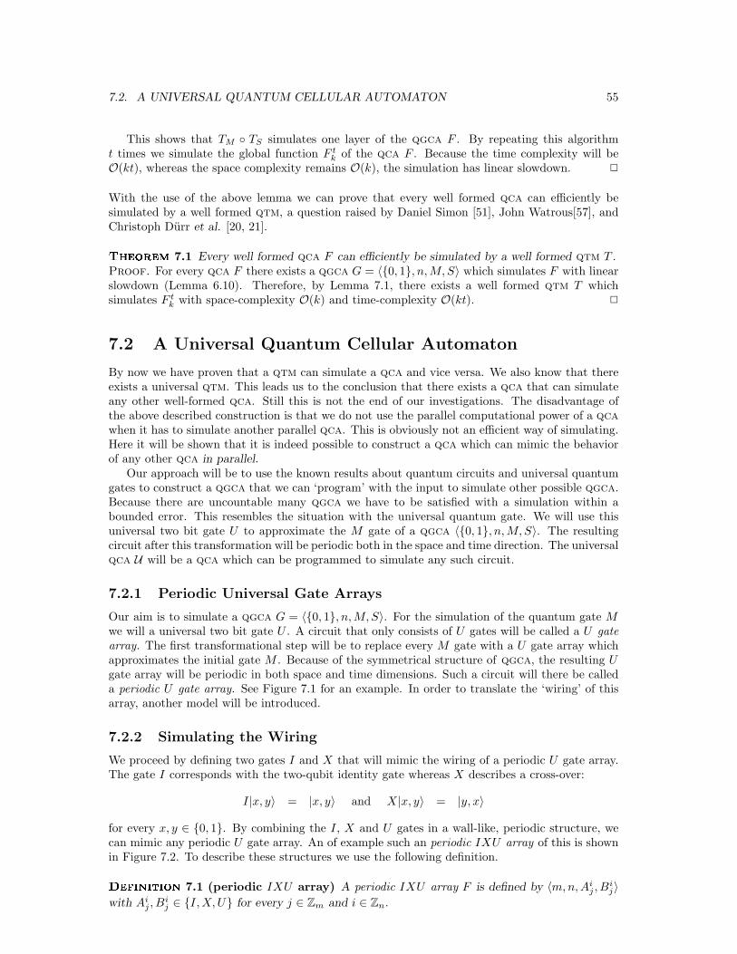
7.2. A UNIVERSAL QUANTUM CELLULAR AUTOMATON 55
This shows that TM ◦ TS simulates one layer of the qgca F . By repeating this algorithmt times we simulate the global function F t
k of the qca F . Because the time complexity will beO(kt), whereas the space complexity remains O(k), the simulation has linear slowdown. 2
With the use of the above lemma we can prove that every well formed qca can efficiently besimulated by a well formed qtm, a question raised by Daniel Simon [51], John Watrous[57], andChristoph Durr et al. [20, 21].
�������7.1 Every well formed qca F can efficiently be simulated by a well formed qtm T .
Proof. For every qca F there exists a qgca G = 〈{0, 1}, n,M, S〉 which simulates F with linearslowdown (Lemma 6.10). Therefore, by Lemma 7.1, there exists a well formed qtm T whichsimulates F t
k with space-complexity O(k) and time-complexity O(kt). 2
7.2 A Universal Quantum Cellular Automaton
By now we have proven that a qtm can simulate a qca and vice versa. We also know that thereexists a universal qtm. This leads us to the conclusion that there exists a qca that can simulateany other well-formed qca. Still this is not the end of our investigations. The disadvantage ofthe above described construction is that we do not use the parallel computational power of a qca
when it has to simulate another parallel qca. This is obviously not an efficient way of simulating.Here it will be shown that it is indeed possible to construct a qca which can mimic the behaviorof any other qca in parallel.
Our approach will be to use the known results about quantum circuits and universal quantumgates to construct a qgca that we can ‘program’ with the input to simulate other possible qgca.Because there are uncountable many qgca we have to be satisfied with a simulation within abounded error. This resembles the situation with the universal quantum gate. We will use thisuniversal two bit gate U to approximate the M gate of a qgca 〈{0, 1}, n,M, S〉. The resultingcircuit after this transformation will be periodic both in the space and time direction. The universalqca U will be a qca which can be programmed to simulate any such circuit.
7.2.1 Periodic Universal Gate Arrays
Our aim is to simulate a qgca G = 〈{0, 1}, n,M, S〉. For the simulation of the quantum gate Mwe will a universal two bit gate U . A circuit that only consists of U gates will be called a U gatearray. The first transformational step will be to replace every M gate with a U gate array whichapproximates the initial gate M . Because of the symmetrical structure of qgca, the resulting Ugate array will be periodic in both space and time dimensions. Such a circuit will there be calleda periodic U gate array. See Figure 7.1 for an example. In order to translate the ‘wiring’ of thisarray, another model will be introduced.
7.2.2 Simulating the Wiring
We proceed by defining two gates I and X that will mimic the wiring of a periodic U gate array.The gate I corresponds with the two-qubit identity gate whereas X describes a cross-over:
I|x, y〉 = |x, y〉 and X|x, y〉 = |y, x〉
for every x, y ∈ {0, 1}. By combining the I, X and U gates in a wall-like, periodic structure, wecan mimic any periodic U gate array. An of example such an periodic IXU array of this is shownin Figure 7.2. To describe these structures we use the following definition.
����������7.1 (periodic IXU array) A periodic IXU array F is defined by 〈m,n,Ai
j , Bij〉
with Aij , B
ij ∈ {I,X,U} for every j ∈ Zm and i ∈ Zn.
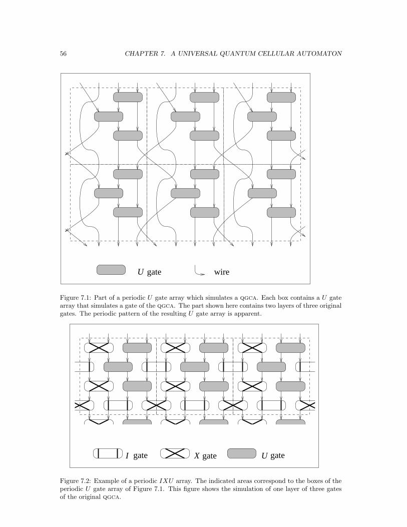
56 CHAPTER 7. A UNIVERSAL QUANTUM CELLULAR AUTOMATON
gate wireU
Figure 7.1: Part of a periodic U gate array which simulates a qgca. Each box contains a U gatearray that simulates a gate of the qgca. The part shown here contains two layers of three originalgates. The periodic pattern of the resulting U gate array is apparent.
gateI X U gategate
Figure 7.2: Example of a periodic IXU array. The indicated areas correspond to the boxes of theperiodic U gate array of Figure 7.1. This figure shows the simulation of one layer of three gatesof the original qgca.
7.2. A UNIVERSAL QUANTUM CELLULAR AUTOMATON 57
A periodic IXU array is build by identical boxes of IXU arrays. The number m indicates thehorizontal size (in terms of gates) of this box whereas n defines the number of double layers ineach box. Each double layer consists of an A layer and a B layer. The function F2mk describesthe behavior of a row Zk of k boxes which acts on 2mk bits and and uses 2n time steps (measuredin individual layers). This function is defined by:
F2mk =
0∏
i=n−1
S† ·
⊗
j∈Zmk
Bijmodm
· S ·
⊗
j∈Zmk
Aijmodm
�������
7.1 The periodic IXU array of Figure 7.2 is defined by 〈2, 2, Aij , B
ij〉 with
A00 = X A0
1 = U
B00 = U B0
1 = I
A10 = X A1
1 = U
B10 = I B1
1 = X
3
Without going into full detail we can state the following lemma.
�����7.2 For every qgca F = 〈{0, 1}, n,M, S〉 there exists a periodic IXU array G =
〈n,m,Aij , B
ij〉 (with gcd(m,n) = 1) which simulates F . This simulation is within an arbitrary
small error.Proof. Use the above described transformation from qgca to periodic U gate arrays to periodicIXU arrays. The gcd(m,n) = 1 constraint is satisfied by adding a sufficient number of identity-layers which only consist of I-gates, thereby increasing the value of n until the desired number isreached. 2
This lemma tells us that for every k ∈ N+ the function G2mk will simulate Fk. If ε indicates theallowed error for simulating one M gate, the simulation of Fk will have an error of kε. Becauseε can be made arbitrary small, kε can be made arbitrary small for a fixed value of k. The linearslowdown is expressed by the ‘vertical size’ of each block which equals 2n. If the simulation of theM gate requires some additional work bits for the U gate array, the space complexity will growwith a factor proportional to k. The reason for the gcd(m,n) = 1 constraint will become evidentin the proof in Appendix D.
If we express the cell values of the periodic IXU array at time t by |xt0, y
t0, . . . , xt
km−1, ytkm−1〉,
the general behavior of the IXU array is calibrated by the equations:
Aimodnjmodm|x2i
j , y2ij 〉 = |x2i+1
j , y2i+1j 〉 (7.1)
Bimodnjmodm|y2i+1
j , x2i+1j+1 〉 = |y2i+2
j , x2i+2j+1 〉 (7.2)
for every i ∈ N and j ∈ Zkm. We will use this ‘calibration’ to prove that the universal automatonU embeds the same behavior.
7.2.3 The Universal Quantum Cellular Automaton
The universal quantum cellular automaton U is described by the following definition (an explana-tion of its semantics will be given below):
����������7.2 (U automaton) The U automaton is a qgca 〈Q,n,M,P 〉 with:
state set Q = {0, 1, /,¤, pIq, pXq, pUq} and n = 4
58 CHAPTER 7. A UNIVERSAL QUANTUM CELLULAR AUTOMATON
quantum gate M : HQ4 → HQ4 that obeys:
M |¤,¤, pAq,¤〉 = |¤,¤, pAq,¤〉 M |¤, x, pAq,¤〉 = |¤, x, pAq,¤〉M |¤,¤, pAq, x〉 = |x,¤, pAq,¤〉 M |¤,¤, pAq, /〉 = |/,¤, pAq,¤〉M |x,¤, pAq, /〉 = |/, x, pAq,¤〉 M |¤, x, pAq, y〉 = |x′,¤, pAq, y′〉
for every x, y ∈ {0, 1} and for every A ∈ {I,X,U}:
A|x, y〉 = |x′, y′〉
neighborhood-scheme P = 〈n, σ, φ〉 defined by
σ(0) = 3 σ(1) = 1 σ(2) = 2 σ(3) = 0
φ(0) = −1 φ(1) = 0 φ(2) = 0 φ(3) = 1
If we supply this automaton with the appropriate input, it will simulate a periodic IXU array.This is shown in the following analysis.
For every N,K ∈ N+ the input:
∣∣∣∣
[
¤x0Jπ0
J¤, y0J¤π1
J¤,¤¤π2J¤, /¤π3
J¤,[¤¤πi
J¤]2N−1
i=4
]
J∈ZK
⟩
with π ∈ {pIq, pXq, pUq} and x, y ∈ {0, 1}, will evolve after two layers of the automaton U2NK
to the configuration:
∣∣∣∣
[
¤¤π0J¤, /y1
Jπ1J¤,
[¤¤πi
J¤]2N−2
i=2, x1
J+1¤π2N−1J ¤
]
J∈ZK
⟩
with Π0J |x0
J , y0J 〉 = |x1
J , x1J 〉 (the gate Π is determined by π0
J = pΠ0Jq). At this point the x-values
will travel step-by-step to the left, while the y-values have moved one place to the right and arenow stationary (this is established by the “/”-symbol).
The next important situation occurs after Θ(N) layers when the x and y values ‘meet again’at the π1
J gates, which are then to be simulated. This will result in the configuration:
∣∣∣∣
[
y2J¤π0
J¤,¤¤π1J¤, /x2
J+1π2J¤,
[¤¤πi
J¤]2N−1
i=2
]
J∈ZK
⟩
with Π1J |y1
J , x1J+1〉 = |y2
J , x2J+1〉 and π1
J = pΠ1Jq.
By now the y-values go left in order to collide at the π2J gates with the x-variables. This process
will be repeated in the obvious way.A careful examination of the behavior of U2NK on this input reveals that the overall time
evolution is calibrated by the equations:
Π2imod2NJ+b 2i
2NcmodK |x2i
J+i, y2iJ+i〉 = |x2i+1
J+i , y2i+1J+i 〉 (7.3)
Π2i+1mod2N
J+b 2i+12N
cmodK|y2i+1
J+i , x2i+1J+i+1〉 = |y2i+2
J+i , y2i+2J+i+1〉 (7.4)
for every i ∈ N, J ∈ ZK , and π·· = pΠ·
·q.By using the calibrations 7.1, 7.2, 7.3, and 7.4, we can prove the following lemma.
�����7.3 Every periodic IXU array F = 〈m,n,Ai
j , Bij〉 with gcd(m,n) = 1 can be simulated
by the qgca U . The time-complexity of the simulation is linear and does not depend on the sizek of the periodic IXU array F2mk.Proof. If a ‘mapping’ between the four calibrations is possible, it follows that the two automatahave the same evolution. Because gcd(m,n) = 1, there exists a positive integer α such that
7.3. CONCLUSIONS 59
αn mod m = 1. With N = αn and K = km every F2mk can be simulated by U2NK . This is shownby the existence of a mapping which satisfies (assuming J = j − i):
Aimodnjmodm = Π2imod2N
j−i+b 2i2N
cmodK Bimodnjmodm = Π2i+1mod2N
j−i+b 2i+12N
cmodK
for every i ∈ N and j ∈ Z. See Appendix D for the existence proof of such a mapping. Because αdoes not depend on k, the time-complexity is bounded by Θ(Ni) = Θ(i) for the simulation of 2ilayers of F . 2
With this lemma we have reached the final conclusion of this thesis.
�������7.2 There exists a proper universal quantum cellular automaton U which can simulate
any well-formed qca F with a bounded error. The extra costs of the simulation of F tk has time-
complexity Θ(t) and space-complexity Θ(k).Proof. This follows from the results of Lemma 6.10, Lemma 7.2 and Lemma 7.3. 2
7.3 Conclusions
We have defined a class of well-formed quantum cellular automata which are one-dimensional andcircular bounded. It has been shown that every proper qca resembles a periodic quantum gatearray. This assures us that the global unitarity of a qca can be reduced to the local unitarityof the gates of a qgca. There exists a qca U which can simulate any such array (by using auniversal two-qubit gate U). The time-complexity of this simulation does not depend on the sizek of the initial qca. This proves that U is a universal quantum cellular automaton.
The existence of a classical universal cellular automata was shown by Jurgen Albert et al. [1]and Bruno Martin [37]. Both constructions did applied to irreversible ca. Because the classicalreversible cellular automata (rca) are a subset of qca, we know that every rca can be simulatedby the non-classical U automaton. If we want a universal rca, we have to adapt Definition7.2 in such a way that it uses a universal three-bit gate (the Toffoli-gate for example). Thisis because there does not exist a classical two-bit gate U that is universal in its computationalpower[3, 4, 16, 18]. The author is unknown of an earlier construction of such an automaton.
Theorem 7.2 shows that the model of qca is a useful model of parallel quantum computingon its own. Because of their uniform structure, cellular automata are particular useful to bridgethe gap between physics and computational theory. From this intermediate standpoint there areat least two directions possible, each with its own merits. By going from qca to physics oneobtains a powerful model to describe quantum mechanical systems. Recent work by David Meyer[39, 40, 41, 42] goes along this pathway.
The other direction is to try to actually construct a controllable qca. Several authors havesuggested that qca-like systems are more likely to be build than quantum Turing machines orientedstructures [8, 34, 35, 36]. If such a construction would indeed be possible in the future, we wouldhave equipped ourselves with a new remarkable tool. A tool whose computational power we arejust beginning to unravel [11, 22, 56].
Appendix A
Unitary Transformations
Because of their central role in quantum computing, we will summarize the properties of unitarytransformations [13, 25, 33, 47]. A linear transformation F is determined by its state set S andthe corresponding transformational matrix MF ∈ CS×S . We will only look at countable state sets.
����������A.1 A transformation F on S is unitary if and only if its corresponding matrix MF
obeys: M†F MF = MF M†
F = 1S , with 1S the identity on the set S.
A.1 Finite dimensional Transformations
If MF is finite dimensional (e.g. S is finite) M†F MF = 1S always implies MF M†
F = 1S . Wetherefore can simplify the above definition.
����������A.2 A finite dimensional transformation F on S is unitary if and only if its corre-
sponding matrix MF obeys: M†F MF = 1S , with 1S the identity on the set S.
A.2 Infinite dimensional Transformations
If we take the the infinite transformation F (i) = i + 1 on S = N we obtain the following ‘inverse’F † : N+ → N, with F †(i+1) = i for every i ∈ N. We therefore have: F †◦F = I but not F ◦F † = I(F ◦ F †(0) is not defined). In matrix notation this is illustrated by:
M†F · MF =
0 1 0 · · ·0 0 1 · · ·0 0 0 · · ·...
......
. . .
·
0 0 0 · · ·1 0 0 · · ·0 1 0 · · ·...
......
. . .
=
1 0 0 · · ·0 1 0 · · ·0 0 1 · · ·...
......
. . .
but:
MF · M†F =
0 0 0 · · ·1 0 0 · · ·0 1 0 · · ·...
......
. . .
·
0 1 0 · · ·0 0 1 · · ·0 0 0 · · ·...
......
. . .
=
0 0 0 · · ·0 1 0 · · ·0 0 1 · · ·...
......
. . .
A closer look at F reveals that F could not be unitary because F is not surjective. This is anecessary and sufficient restriction for infinite transformations with M†
F MF = 1S to be unitary:
����������A.3 An infinite dimensional transformation F on S is unitary if and only if its
corresponding matrix MF obeys: M†F MF = 1S (with 1S the identity on the set S) and F is
surjective.
60
A.3. EXPONENTIAL EXPRESSIONS 61
A.3 Exponential Expressions����������
A.4 Let H be a square matrix, by eH we mean I + H + 12H2 + · · · . Therefore for
every t ∈ C:
exp(t · H) =
∞∑
k=0
1
k!· tk · Hk
�������
A.1
exp
(
t ·(
0 ii 0
))
=
(cos(t) i sin(t)i sin(t) cos(t)
)
3
����������A.5 A matrix A is called hermitian if and only if A† = A.
Finite unitary and hermitian matrix correspond to each other in the following way.
1. For every hermitian matrix H, exp(iH) is a unitary matrix.
2. For every unitary matrix U , there exists a hermitian matrix H such that: U = exp(iH) (ingeneral this H is not unique).
For this reason the analogy of hermitian matrices to real numbers and unitary matrices to thecomplex numbers with norm one is made (except for commutativity of multiplication).
Appendix B
Proving Well-Formedness
In this appendix we will prove that if the general function FZ of a normalized qca is not well-formed, there exists a K ∈ N+ such that Fk is not unitary. This result is used in Lemma 4.3.
�����B.1 Let F = 〈Q,N, f〉 a normalized qca. If there exist two values X 6= Y ∈ QZ such
that
〈FZ(X)i, FZ(Y )i〉 6= 0
for every i ∈ Z, then there exists a k ∈ N+ with Fk not unitary.Proof. We use xi and yi ∈ HQ defined by
FZ(X) = FZ
(⊗
i∈Z
Xi
)
=⊗
i∈Z
xi and FZ(Y ) = FZ
(⊗
i∈Z
Yi
)
=⊗
i∈Z
yi
with Xi, Yi ∈ Q and X0 6= Y0 such that
for every i ∈ Z : 〈xi, yi〉 6= 0 (B.1)
We will now prove that, given these X and Y , we are able to construct a k ∈ N+ and a X ′, Y ′ ∈ Qk,with X ′ ⊥ Y ′ and Fk|X ′〉 6⊥ Fk|Y ′〉.
Define r = |N | the size of the normalized neighborhood N = {0, 1, . . . , r − 1}. Take a, b, c andd (with a < b ≤ 0 ≤ c < d), such that:
Xa:(a+r−1) = Xb:(b+r−1) Ya:(a+r−1) = Yb:(b+r−1)
Xc:(c+r−1) = Xd:(d+r−1) Yc:(c+r−1) = Yd:(d+r−1)
Because there are ‘only’ |Q|2r different combinations of [Xi:(i+r−1);Yi:(i+r−1)], this is always pos-sible for a ≥ −|Q|2r and d ≤ |Q|2r. With these values we define:
XL = Xa:(b−1) XR = Xc:(d−1)
YL = Ya:(b−1) YR = Yc:(d−1)
This can be visualized by:
X = · · ·XL
︷ ︸︸ ︷
Xa ⊗ · · · ⊗ Xb−1 ⊗Xb ⊗ · · · ⊗ X0 ⊗ · · · ⊗XR
︷ ︸︸ ︷
Xc ⊗ · · · ⊗ Xd−1 ⊗Xd · · ·Y = · · · Ya ⊗ · · · ⊗ Yb−1
︸ ︷︷ ︸
YL
⊗Yb ⊗ · · · ⊗ Y0 ⊗ · · · ⊗ Yc ⊗ · · · ⊗ Yd−1︸ ︷︷ ︸
YR
⊗Yd · · ·
Now we distinguish the following three possibilities:
62
63
1. XL 6= YL: Take X ′ = XL, Y ′ = YL both elements of Qk with k = b− a (thus X ′ ⊥ Y ′). For0 ≤ i ≤ r − 1 we have:
X ′k+i = X ′
i = Xa+i = Xb+i
and therefore:
Fk(X ′) =⊗
j∈Zk
f
(⊗
i∈Zr
X ′j+i
)
=⊗
j∈Zk
f
(⊗
i∈Zr
Xa+j+i
)
= (FZ(X))a:(b−1)
and for the same reasons also: Fk(Y ′) = (FZ(Y ))a:(b−1). This leads us to:
〈Fk(X ′), Fk(Y ′)〉 =⟨
(FZ(X))a:(b−1) , (FZ(Y ))a:(b−1)
⟩
=b−1∏
i=a
〈xi, yi〉
By (B.1) we now know that Fk(X ′) 6⊥ Fk(Y ′), which shows that Fk is not a unitary trans-
formation (with k ≤ |Q|2r).
2. XR 6= YR: With X ′ = XR, Y ′ = YR and k = d − c, the same reasoning as with XL 6= YL
holds (again k ≤ |Q|2r).
3. XL = YL and XR = YR: First we will prove Xa:(b+r−1) = Ya:(b+r−1). We already know:Xa:(b−1) = Ya:(b−1). With induction (given 0 ≤ i ≤ r − 1 and Xa:(b+i−1) = Ya:(b+i−1))it follows that Xb+i = Xa+i = Ya+i = Yb+i holds. Likewise we can prove: Xc:(d+r−1) =
Yc:(d+r−1). Now take X ′ = Xb:(c+r−1) and Y ′ = Yb:(c+r−1) ∈ Qk, with k = c + r − b.Because b ≤ 0 ≤ c + r − 1 and X0 6= Y0, we have X ′ ⊥ Y ′. Below we will use: (becauseXb:(b+r−1) = Yb:(b+r−1) and Xc:(c+r−1) = Yc:(c+r−1)):
for every 0 ≤ i ≤ r − 1 : X ′c−b+i = Xc+i = Yc+i = Y ′
c−b+i
and also for every r ≤ i ≤ 2r − 2:
X ′c−b+i = X ′
k+i−r = X ′i−r = Xb+i−r = Yb+i−r = Y ′
i−r = Y ′k+i−r = Y ′
c−b+i
To summarize: X ′c−b+i = Y ′
c−b+i; if 0 ≤ i ≤ 2r − 2. This gives us:
Fk(X ′) =⊗
j∈Zk
f
(⊗
i∈Zr
X ′j+i
)
=
c−b−1⊗
j=0
f
(⊗
i∈Zr
X ′j+i
)
⊗
k−1⊗
j=c−b
f
(⊗
i∈Zr
X ′j+i
)
=
c−1⊗
j=b
f
(⊗
i∈Zr
Xj+i
)
⊗
k−1⊗
j=c−b
f
(⊗
i∈Zr
Y ′j+i
)
If we combine this with:
Fk(Y ′) =
c−1⊗
j=b
f
(⊗
i∈Zr
Yj+i
)
⊗
k−1⊗
j=c−b
f
(⊗
i∈Zr
Y ′j+i
)
64 APPENDIX B. PROVING WELL-FORMEDNESS
the inner-product of Fk(X ′) and Fk(Y ′) equals:
〈Fk(X ′), Fk(Y ′)〉 =
⟨
c−1⊗
j=b
f
(⊗
i∈Zr
Xj+i
)
,
c−1⊗
j=b
f
(⊗
i∈Zr
Yj+i
)
⟩
=⟨
(FZ(X))b:(c−1) , (FZ(Y ))b:(c−1)
⟩
=
c−1∏
i=b
〈xi, yi〉
Again, (B.1) shows us that Fk(X ′) 6⊥ Fk(Y ′), which shows that Fk is not a unitary trans-
formation (with k ≤ 2|Q|2r+ r).
All possibilities are covered by 1, 2 and 3. This proves that there exists a k ≤ 2|Q|2r+r, for which
Fk is not unitary: the qca F is not well-formed as defined in (4.7). 2
Appendix C
Simulating Neighborhood Schemes
In this appendix we give the proof of Lemma 6.6 about the simulation of arbitrary neighborhoodschemes by periodic qgca which only use the Shift neighborhood scheme.
�����C.1 For every qgca F = 〈Q,n,M,P 〉 there exists a periodic qgca G defined by
G = 〈Q,n, µ,M0, . . . ,Mµ−1, S, . . . , S〉
which is shift equivalent with F .Proof. Given the neighborhood scheme P = 〈n, σ, φ〉, we will use the labels:
• Φ = {φ(i) | i ∈ Zn}
• r = max(Φ) − min(Φ)
• ψi = {σ(t) | t ∈ Zn and φ(t) = min(Φ) + i} for every 0 ≤ i ≤ r
• m(P ) =∑r
i=0 i · |ψi|
(Therefore if m(P ) = 0 we have ψ0 = Zn and m(P ) = 1 implies |ψ0| = n − 1 and |ψ1| = 1.)For every neighborhood scheme P = 〈n, σ, φ〉 and value c ∈ Zn, we define the following standardprocedure:
Construct an alternative neighborhood scheme R = 〈n, ς, ϕ〉 by
ς(i) = σ(i) and ϕ(i) = φ(i) − 1c(i)
Next, we define two ’permutation gates’ Π : Zn → Zn and π : Zn → Zn by:
Π(i) =
n − 1 if i = cc if i = n − 1i otherwise
and π(i) = Π(i − 1) (such that π(Π(i) + 1) = i for every i ∈ Zn). We now have for every k ∈ N+:
Π[k] ◦ Sk ◦ π[k] ◦ Rk = 〈n,Π(i), 0〉 ◦ 〈n, i + 1, 1n−1(i)〉 ◦ 〈n, π(i), 0〉 ◦ 〈n, ς(i), ϕ(i)〉= 〈n,Π(i), 0〉 ◦ 〈n, i + 1, 1n−1(i)〉 ◦ 〈n, ς ◦ π(i), ϕ ◦ π(i)〉= 〈n,Π(i), 0〉 ◦ 〈n, ς ◦ π(i + 1), 1n−1(i) + ϕ ◦ π(i + 1)〉= 〈n, ς ◦ π(Π(i) + 1), 1n−1 ◦ Π(i) + ϕ ◦ π(Π(i) + 1)〉= 〈n, σ(i), φ(i)〉= Pk
This shows that the µ + 1-periodic qgca G′ = 〈Q,n, µ + 1, π,M0 ◦ Π, . . . ,Mµ−1, R, S, . . . , S〉 isidentical with the µ-periodic qgca G = 〈Q,n, µ,M0, . . . ,Mµ−1, P, S, . . . , S〉, and thus G = G′.
65
66 APPENDIX C. SIMULATING NEIGHBORHOOD SCHEMES
We will use this procedure to ‘transform’ the qgca F into the desired periodic qgca. For everyµ-periodic qgca G = 〈Q,n, µ,M0, . . . ,Mµ−1, P, S, . . . , S〉, we distinguish the following (mutualexclusive) possibilities:
1. {0} = ψ0 and n = 1: The neighborhood scheme P = 〈n, σ, φ〉 has σ(0) = 0 and φ(0) = t(with t ∈ Z). We therefore have S ◦St−1 = Pk for every k ∈ N+. This proves the µ-periodicqgca G′ = 〈Q,n, µ,M0, . . . ,Mµ−1, S, . . . , S〉 to be shift-equivalent with the initial qgca
G; in other words G′ ≡ G.
2. {0} = ψ0 and n > 1: Take c such that σ(c) = max(Ψ) and apply the procedure. The newneighborhood scheme R has m(R) = m(P ) − 1.
3. {0} ( ψ0: Take c with σ(c) 6= 0 and φ(c) = min(Ψ) and apply the procedure to getthe neighborhood scheme R. Now we have ψR
0 = {ς(c)} = {σ(c)} + {0} combined withm(R) = m(P ) + n − 1.
4. {0} * ψ0 and m(P ) > 1: Take c such that σ(c) = max(ψr) and apply the procedure. Forthe neighborhood scheme R we have m(R) = m(P ) − 1 and (again) {0} * ψR
0 .
5. {0} * ψ0 and m(P ) = 1: This implies: ψ0 = {1, . . . , n − 1}; ψ1 = {0}; Φ = {t, t + 1};φ(c) = t + 1; σ(c) = 0, with t ∈ Z and c ∈ Zn (therefore φ(i) = t + 1c(i)). Define thepermutation-gate Π(i) = σ(i) − 1. It now holds for every k ∈ N+:
Π[k] ◦ Sk ◦ Stnk = 〈n,Π(i), 0〉 ◦ 〈n, i + 1, 1n−1(i)〉 ◦ 〈n, i, t〉
= 〈n,Π(i) + 1, 1n−1(Π(i))〉 ◦ 〈n, i, t〉= 〈n, σ(i), 1c(i) + t〉= Pk
This shows that if we define a µ-periodic qgca
G′ = 〈Q,n, µ,M0 · Π,M1, . . . ,Mµ−1, S, . . . , S〉
we have finally reached the shift-equivalence G ≡ G′.
If we start with the initial qgca F and apply the above transformation recursively, we will alwaysreach (after a finite amount of steps) possibility 5. This means that we have constructed thedesired µ-periodic qgca G, with F ≡ G. 2
Appendix D
Mapping the Calibrations
We will prove the existence of a mapping as used in Lemma 7.3.
�����D.1 For every m,n ∈ N+ with gcd(m,n) = 1, there exists an α ∈ N∗ and a mapping Π·
·
of A·· and B·
· which respects the equations (with N = αn and K = km)
Aimodnjmodm = Π2imod2N
j−i+b 2i2N
cmodK Bimodnjmodm = Π2i+1mod2N
j−i+b 2i+12N
cmodK
for every i, k ∈ N and j ∈ Z.Proof. In order to ensure a correct mapping between the A values and Π, we have to prove thatif:
2i mod 2N ≡ 2p mod 2N
j − i +
⌊2i
2N
⌋
mod K ≡ q − p +
⌊2p
2N
⌋
mod K
then:
i mod n ≡ p mod n
j mod m ≡ q mod m
for every i, p ∈ N and j, q ∈ Z.By K = km and defining α such that N = αn ≡ 1 mod m, the initial conditions can be
restated to:
2(i − p) mod 2αn ≡ 0
(j − q) − (i − p) +
⌊2i
2αn
⌋
−⌊
2p
2αn
⌋
mod km ≡ 0
The first condition leads to p = i + λαn (with λ ∈ Z). As a result the second condition becomes:
(j − q) + λ(αn − 1) mod km ≡ 0
Therefore the the restrictions (i − p) mod n ≡ 0 and (j − q) mod m ≡ 0 are satisfied for everyi, p ∈ N and j, q ∈ Z.
The same reasoning holds if we want to prove the existence of a consistent mapping betweenthe B values and Π. 2
67
Appendix E
Sources of Information
The writing of this thesis has benefited greatly from the information which is nowadays available onthe internet. The pace of the recent developments in quantum computing is unthinkable withoutthe existence of archives such as quant-ph or qcomp. What follows is a personal selection of thesites and home-pages which I found particular useful.
http://xxx.lanl.gov/archives/quant-ph
The e-print archive of the Los Alamos National Laboratory has shown to be the center ofpublications regarding quantum computation.
http://babbage.sissa.it/quant-ph/
The European mirror-site of quant-ph.
http://feynman.stanford.edu/qcomp/
The Quantum Computation Archive at the Stanford University provides a large but well-selected database of articles solely about quantum computation.
http://eve.physics.ox.ac.uk/QChome.html
The home-page of the Quantum Information Group at the University of Oxford. With on-line elementary introductions about quantum cryptography, cryptoanalysis, computationand communication by Artur Ekert and David Deutsch.
http://vesta.physics.ucla.edu/~smolin/index.html
The colorful Quantum Information Page of John Smolin at University of California, Los An-geles.
http://www.cwi.nl/~berthiau/
Andre Berthiaume’s home-page with his introduction in quantum computation [7].
http://www.iro.umontreal.ca/labs/theorique/index_en.html
The Laboratory for Theoretical & Quantum Computing at the Universite de Montreal. GillesBrassard’s extensive Bibliography of Quantum Cryptography can be found at the Englishhome-page of Claude Crepeau.
http://www.research.ibm.com/quantuminfo/
The research group at IBM with an on-line article about quantum teleportation.
http://www.physik.uni-ulm.de/~sam/home.html
Starting point of the tutorial on quantum computation by Samuel Braunstein.
http://publish.aps.org/PRA/prahome.html
Site of Physical Review A, the journal where the field of quantum computation has foundits niche.
68
69
http://alife.santafe.edu/alife/topics/cas/ca-faq/ca-faq.html
Frequently Asked Questions about cellular automata; edited by Howard Gutowitz. Keepsalso track of the ongoing discussions in the newsgroup comp.theory.cell-automata.
http://cs.ua.edu/graduate/lusth/qca/
The Quantum Coupled Architecture Home Page which deals with a number of subjectsclosely related to qca.
http://aerodec.anu.edu.au/~qc/index.html
The Quantum Computing home page of the Australian National University, including a listof paper reviews.
http://altavista.digital.com/
“If all else fails, try consulting AltaVista.” Current statistics (Summer 1996):
• “cellular automata”: 5037 documents matching the query
• “quantum computation”: 990 documents matching the query
• “quantum cellular automata”: 40 documents matching the query
Bibliography
[1] Jurgen Albert and Karel Culik II. A simple universal cellular automaton and its one-way andtotalistic version. Complex Systems, 1:1–16, 1987.
[2] Serafino Amoroso and Yale N. Patt. Decision procedures for surjectivity and injectivity ofparallel maps for tessellation structures. Journal of Computer and System Sciences, 6(5):448–464, October 1972.
[3] Adriano Barenco. A universal two-bit gate for quantum computation. Proceedings of the RoyalSociety of London A, 449:669–677, 1995. http://xxx.lanl.gov/abs/quant-ph/9505016.
[4] Adriano Barenco, Charles H. Bennett, Richard Cleve, David P. DiVincenzo, Norman Margo-lus, Peter Shor, Tycho Sleator, John Smolin, and Harald Weinfurter. Elementary gates forquantum computation. Physical Review A, 52(5):3457–3467, 1995. http://xxx.lanl.gov/
abs/quant-ph/9503016.
[5] Charles H. Bennett. Logical reversibility of computation. IBM Journal of Research andDevelopment, 17:525–532, November 1973.
[6] Ethan Bernstein and Umesh Vazirani. Quantum complexity theory. In Proceedings of the 25thAnnual ACM Symposium on Theory of Computing, pages 11–20, San Diego, California, May1993. ACM Press. ftp://math.berkeley.edu/pub/Preprints/Bob_Solovay/Quantum/.
[7] Andre Berthiaume. Quantum computation. In Complexity Theory Retrospective II. Springer-Verlag, 1996. To appear. http://www.cwi.nl/~berthiau/seminar.html.
[8] Michael Biafore. Can quantum commputers have simple Hamiltonians? http://dynamics.
bu.edu/InterJournal/papers/[3]_120994152541_.html, November 1994. Presented atPhysics and Computation 1994.
[9] Michel Boyer, Gilles Brassard, Peter Høyer, and Alain Tapp. Tight bounds on quantumsearching. http://xxx.lanl.gov/abs/quant-ph/9605034, May 1996. To be appear in theconference proceedings of Physics and Computation 1996.
[10] Brian H. Bransden and Charles J. Joachain. Introduction to Quantum Mechanics. LongmanScientific & Technical, New York, 1989.
[11] Gilles Brassard. Quantum computing: The end of classical cryptography? SIGACT News,25(4):15–21, December 1994. Cryptology column.
[12] Arthur W. Burks, editor. Essays on Cellular Automata. University of Illinois Press, Urbana,1970.
[13] Richard Courant and David Hilbert. Methods of Mathematical Physics, volume 1. IntersciencePublishers, New York, 1953.
[14] Ashok Das and Adrian C. Melissinos. Quantum Mechanics: a modern introduction. Gordonand Breach Science Publishers, New York, 1986.
70
BIBLIOGRAPHY 71
[15] David Deutsch. Quantum theory, the Church–Turing principle and the universal quantumcomputer. Proceedings of the Royal Society of London A, 400:97–117, 1985.
[16] David Deutsch. Quantum computational networks. Proceedings of the Royal Society of LondonA, 425:73–90, 1989.
[17] Paul A.M. Dirac. The Principles of Quantum Mechanics. Clarendon Press, Oxford, fourthedition, 1958.
[18] David P. DiVincenzo. Two-bit gates are universal for quantum computation. Physical ReviewA, 51(2):1015–1022, 1995. http://xxx.lanl.gov/abs/cond-mat/9407022.
[19] Jean-Christphe Dubacq. How to simulate non-reversible turing machines by one-dimensionalcellular automata. Technical Report URA CNRS 1398, Ecole Normale Superieure de Lyon,Laboratoire d’informatique du Parallelisme, March 1995.
[20] Christoph Durr and Miklos Santha. A decision procedure for unitary linear quantum cellularautomata. In Proceedings of the 37th Annual Symposium on Foundations of Computer Sci-ence. IEEE Computer Society Press, October 1996. http://xxx.lanl.gov/abs/quant-ph/
9604007.
[21] Christoph Durr, Huong Le Thanh, and Miklos Santha. A decision procedure for well-formedquantum linear cellular automata. In Claude Puech and Rudiger Reischuk, editors, 13thAnnual Symposium on Theoretical Aspects of Computer Science, volume 1046 of LectureNotes in Computer Science, pages 281–292. Springer, February 1996.
[22] Artur Ekert. Quantum computation. http://feynman.stanford.edu/qcomp/ekert/index.html, 1994. Proceedings of the ICAP meeting, Boulder.
[23] Doyne Farmer, Tommaso Toffoli, and Stephen Wolfram, editors. Cellular Automata, vol-ume 10(1,2) of Physica D, North-Holland, Amsterdam, March 1983. Los Alamos NationalLaboratory, Elsevier Science Publishers.
[24] Richard P. Feynman. The Feynman lectures on physics, volume III: Quantum Mechanics.Addison-Wesley, 1965.
[25] Joel N. Franklin. Matrix Theory. Prentice-Hall, 1968.
[26] Lov G. Grover. A fast quantum mechanical algorithm for database search. In Proceedingsof the 28th Annual Symposium on the Theory of Computing, pages 212–219, Philadelphia,Pennsylvania, May 1996. STOC’96. http://xxx.lanl.gov/abs/quant-ph/9605043.
[27] Howard A. Gutowitz, editor. Cellular automata: Theory and Experiment, volume 45(1,2,3)of Physica D, North-Holland, Amsterdam, September 1990. The Center for Nonlinear Studes;Los Alamos National Laboratory, Elsevier Science Publishers.
[28] Gustav A. Hedlund. Endomorphisms and automorphisms of the shift dynamical system.Mathematical Systems Theory, 3(4):320–375, 1969.
[29] Peter Høyer. Note on linear quantum cellular automata. http://www.imada.ou.dk/~u2pi/,February 1996.
[30] Richard Jozsa. Characterizing classes of functions computable by quantum parallelism. Pro-ceedings of the Royal Society of London A, 435:563–574, 1991.
[31] Jarkko Kari. On the inverse neighborhoods of reversible cellular automata. In GrzegorzRozenberg and Arto Salomaa, editors, Lindenmayer Systems, Impacts on theoretical Com-puter Graphics, and Developmental Biology, pages 477–495. Springer-Verlag, 1992.
72 BIBLIOGRAPHY
[32] Jarkko Kari. Representation of reversible cellular automata with block permutations. Math-ematical Systems Theory, 29(1):47–61, January 1996.
[33] Peter Lancaster. Theory of Matrices. Academic Press, New York, 1969.
[34] Seth Lloyd. A technologically feasible quantum computer. http://feynman.stanford.edu/qcomp/lloyd/index.html.
[35] Seth Lloyd. A potentially realizable quantum computer. Science, 261:1569–1571, 1993.
[36] Norman Margolus. Parallel quantum computation. In Wojciech H. Zurek, editor, Complexity,Entropy, and the Physics and Information, volume VIII of SFI Studies in the Sciences of Com-plexity, pages 273–287. Addison–Wesley, Redwood City, 1990. http://feynman.stanford.
edu/qcomp/margolus/index.html.
[37] Bruno Martin. A universal cellular automaton in quasi-linear time and its S–m–n form.Theoretical Computer Science, 123:199–237, 1994.
[38] Akira Maruoka and Masayuki Kimura. Condition for injectivity of global maps for tessellationautomata. Information and Control, 32:158–162, 1976.
[39] David A. Meyer. From quantum cellular automata to quantum lattice gases. http://xxx.
lanl.gov/abs/quant-ph/9604003, March 1996. To appear in Journal of Statistical Physics.
[40] David A. Meyer. On the absence of homogeneous scalar quantum cellular automata. http:
//xxx.lanl.gov/abs/quant-ph/9604011, April 1996. Submitted to Physics Letters A.
[41] David A. Meyer. Quantum mechanics of lattice gas automata I. One particle plane waves andpotentials. Private communication, July 1996. Submitted to Physical Review E.
[42] David A. Meyer. Unitarity in one dimensional nonlinear quantum cellular automata.http://xxx.lanl.gov/abs/quant-ph/9605023, April 1996. Submitted to Communicationsin Mathematical Physics.
[43] Marvin Minsky. Computation: finite and infinite machines. Prentice-Hall International,London, 1967.
[44] Kenichi Morita. Computation-universality of one-dimensional one-way reversible cellular au-tomata. Information Processing Letters, 42:325–329, July 1992.
[45] Kenichi Morita and Masateru Harao. Computation universality of one-dimensional reversible(injective) cellular automata. Transactions of the IEICE, E72(6):758–762, June 1989.
[46] John von Neumann. Theory of Self-Reproducing Automata. University of Illinois Press,Urbana, 1966. Edited and completed by Arthur W. Burks.
[47] Marshall C. Pease III. Methods of Matrix Algebra. Mathematics in Science and Engineering16. Academic Press, New York, 1965.
[48] Daniel Richardson. Tesselations with local transformations. Journal of Computer and SystemSciences, 6(5):373–388, October 1972.
[49] Peter W. Shor. Algorithms for quantum computation: Discrete logarithms and factoring.In Shafi Goldwasser, editor, Proceedings of the 35th Annual Symposium on Foundations ofComputer Science, pages 124–134. IEEE Computer Society Press, November 1994. http:
//feynman.stanford.edu/qcomp/shor/index.html.
[50] Peter W. Shor. Polynomial-time algorithms for prime factorization and discrete logarithmson a quantum computer. http://xxx.lanl.gov/abs/quant-ph/9508027, August 1995. Ex-panded version of [49].
BIBLIOGRAPHY 73
[51] Daniel R. Simon. On the power of quantum computation. In Shafi Goldwasser, editor, Pro-ceedings of the 35th Annual Symposium on Foundations of Computer Science, pages 116–123.IEEE Computer Society Press, November 1994. http://feynman.stanford.edu/qcomp/
simon/index.html.
[52] Tommaso Toffoli. Computation and construction universality of reversible cellular automata.Journal of Computer and System Sciences, 15:213–231, 1977.
[53] Tommaso Toffoli. Cellular automata as an alternative to (rather than an approximation of)differential equations in modeling physics. Physica D, 10:117–127, 1984. Contribution in [23].
[54] Tommaso Toffoli and Norman Margolus. Cellular automata machines: a new enviroment formodeling. MIT Press, Cambridge, 1987.
[55] Tommaso Toffoli and Norman Margolus. Invertible cellular automata: a review. Physica D,45:229–253, 1990. Contribution in [27].
[56] Paul Vitanyi. Physics and the new computation. In Jirı Wiedermann and Petr Hajek, editors,Mathematical Foundations of Computer Science 1995, Proceedings of the 20th InternationalSymposium, volume 969 of Lecture Notes in Computer Science, pages 106–128. Springer,August 1995. http://www.cwi.nl/~paulv/publications.html.
[57] John Watrous. On one-dimensional quantum cellular automata. In Proceedings of the 36thAnnual Symposium on Foundations of Computer Science, pages 528–537, Milwaukee, Wis-consin, October 1995. IEEE Computer Society Press.
[58] Stephen Wolfram. Theory and Applications of Cellular Automata, volume 1 of Advancedseries on complex systems. World Scientific Publishing Co Pte Ltd., 1986.
[59] Stephen Wolfram. Cellular Automata and Complexity. Addison-Wesley, 1994. Collectedpapers.
[60] Andrew Chi-Chih Yao. Quantum circuit complexity. In Proceedings of the 34th IEEE Sympo-sium on Foundations of Computer Science, pages 352–361, 1993. http://feynman.stanford.edu/qcomp/yao/index.html.