quantum computing intro. & overview: what’s quantum computing all about?
TRANSCRIPT
Quantum ComputingQuantum Computing
Intro. & Overview:Intro. & Overview:What’s Quantum Computing All What’s Quantum Computing All
About?About?
Classical Classical vs.vs. Quantum Computing Quantum Computing• For any digital computer, its set of For any digital computer, its set of computational computational
statesstates is some set of mutually distinguishable abstract is some set of mutually distinguishable abstract states.states.– The specific computational state that is in use at a given The specific computational state that is in use at a given
time represents the specific digital data currently being time represents the specific digital data currently being processed within the machine.processed within the machine.
• Classical computingClassical computing is computing in which: is computing in which:– All of the computational states (at all times) are stable All of the computational states (at all times) are stable
pointer states of the computer hardware.pointer states of the computer hardware.
• Quantum computingQuantum computing is computing in which: is computing in which:– The computational state is The computational state is notnot always a pointer state. always a pointer state.
What is “Quantum Computing?”What is “Quantum Computing?”• Non-pointer-state computing.Non-pointer-state computing.• Harnesses these quantum effects on a large, Harnesses these quantum effects on a large,
complex scale:complex scale:– Computational states that are not just pointer states, but Computational states that are not just pointer states, but
also, also, coherent superpositionscoherent superpositions of pointer states. of pointer states.• States having non-zero amplitude in many pointer states at the States having non-zero amplitude in many pointer states at the
same time! “Quantum parallelism.”same time! “Quantum parallelism.”– Entanglement (quantum correlations)Entanglement (quantum correlations)
• Between the states of different subsystems.Between the states of different subsystems.– Unitary (thus reversible) evolution through timeUnitary (thus reversible) evolution through time– Interference (reinforcement and cancellation)Interference (reinforcement and cancellation)
• Between convergent trajectories in pointer-state space.Between convergent trajectories in pointer-state space.
WhyWhy Quantum Computing? Quantum Computing?• It is, It is, apparentlyapparently, exponentially more time-efficient , exponentially more time-efficient
than than any possibleany possible classical computing scheme at classical computing scheme at solving solving somesome problems: problems:– Factoring, discrete logarithms, related problemsFactoring, discrete logarithms, related problems– Simulating quantum physical systems accuratelySimulating quantum physical systems accurately
• This application was the original motivation for quantum This application was the original motivation for quantum computing research first suggested by famous physicist computing research first suggested by famous physicist Richard Feynman in the early 80’s.Richard Feynman in the early 80’s.
• However, this has never been proven yet!However, this has never been proven yet!– If you want to win a sure-fire Nobel prize…If you want to win a sure-fire Nobel prize…
• Find a Find a polynomial-timepolynomial-time algorithm for accurately simulating algorithm for accurately simulating quantum computers on classical ones!quantum computers on classical ones!
Status of Quantum ComputingStatus of Quantum Computing• Theoretical & experimental progress is being made, Theoretical & experimental progress is being made,
but slowly.but slowly.– There are many areas where much progress is still needed.There are many areas where much progress is still needed.
• Physical implementations of very small Physical implementations of very small ((e.g.e.g., 7-bit) quantum computers have been tested and , 7-bit) quantum computers have been tested and work as predicted.work as predicted.– However, scaling them up is difficult.However, scaling them up is difficult.
• There are no known There are no known fundamentalfundamental theoretical barriers theoretical barriers to large-scale quantum computing.to large-scale quantum computing.– Guess: It will be a real technology in ~20 yrs. or so.Guess: It will be a real technology in ~20 yrs. or so.
Early HistoryEarly History• Quantum computing was largely inspired by reversible Quantum computing was largely inspired by reversible
computation work from the 1970’s:computation work from the 1970’s:– Bennett, Fredkin, and ToffoliBennett, Fredkin, and Toffoli
• Early quantum computation pioneers (1980’s):Early quantum computation pioneers (1980’s):– Early models not using quantum parallelism Early models not using quantum parallelism
to gain performance:to gain performance:• Benioff ‘80, ‘82 - Quantum serial TM modelsBenioff ‘80, ‘82 - Quantum serial TM models• Feynman ‘86 - Q. models of serial reversible circuitsFeynman ‘86 - Q. models of serial reversible circuits• Margolus ‘86,’90 - Q. models of parallel rev. circuitsMargolus ‘86,’90 - Q. models of parallel rev. circuits
– Performance gains w. quantum parallelism:Performance gains w. quantum parallelism:• Feynman ‘82 - Suggested faster quantum sims with QCFeynman ‘82 - Suggested faster quantum sims with QC• Deutsch ‘85 - Quantum-parallel Turing machineDeutsch ‘85 - Quantum-parallel Turing machine• Deutsch ‘89 - Quantum logic circuitsDeutsch ‘89 - Quantum logic circuits
More Recent HistoryMore Recent History• There was a rapid ramp-up of quantum computing There was a rapid ramp-up of quantum computing
research throughout the 1990’s.research throughout the 1990’s.• Some developments, 1989-presentSome developments, 1989-present
– Refining quantum logic circuit modelsRefining quantum logic circuit models• What is a minimal set of universal gates for QC?What is a minimal set of universal gates for QC?
– Algorithms: Shor factoring, Grover search, etc.Algorithms: Shor factoring, Grover search, etc.– Developing quantum complexity theoryDeveloping quantum complexity theory
• What is the ultimate power of quantum computation?What is the ultimate power of quantum computation?– Quantum information theoryQuantum information theory
• Communications, Cryptography, Communications, Cryptography, etc.etc.• Error correcting codes, fault tolerance, robust QCError correcting codes, fault tolerance, robust QC
– Physical implementationsPhysical implementations• Numerous few-bit implementations demonstratedNumerous few-bit implementations demonstrated
Quantum Logic NetworksQuantum Logic Networks• Invented by Deutsch (1989)Invented by Deutsch (1989)
– Analogous to classical Boolean logic networksAnalogous to classical Boolean logic networks– Generalization of Fredkin-Toffoli reversible logic circuitsGeneralization of Fredkin-Toffoli reversible logic circuits
• System is divided into individual bits, or System is divided into individual bits, or qubitsqubits– 2 orthogonal states of each bit are designated as the 2 orthogonal states of each bit are designated as the
computationalcomputational basis statesbasis states, “0” and “1”., “0” and “1”.
• Quantum logic gates:Quantum logic gates:– Local unitary transforms that operate on only a few state Local unitary transforms that operate on only a few state
bits at a time.bits at a time.
• Computation via predetermined seq. of gate Computation via predetermined seq. of gate applications to selected bits.applications to selected bits.
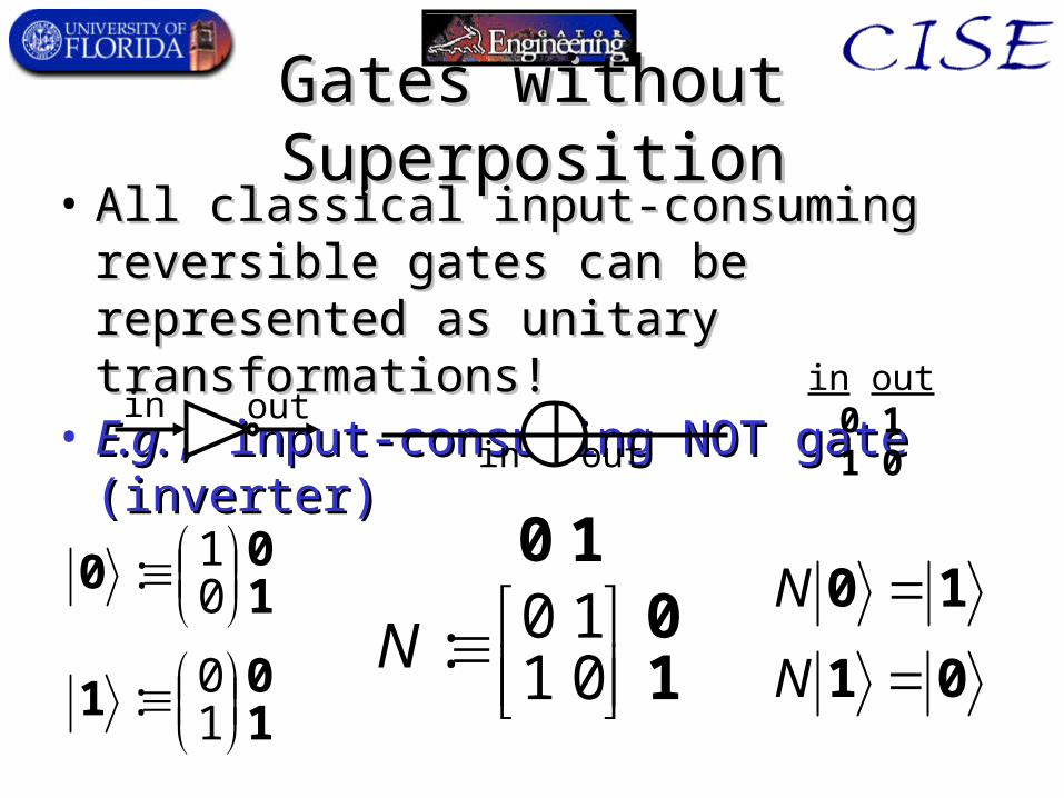
Gates without SuperpositionGates without Superposition• All classical input-consuming reversible gates All classical input-consuming reversible gates
can be represented as unitary transformations!can be represented as unitary transformations!• E.g.E.g., input-consuming NOT gate (inverter), input-consuming NOT gate (inverter)
in outin out
in out0 11 0
10
10
01
10:N 01
10
N
N
101
100
10:
01:
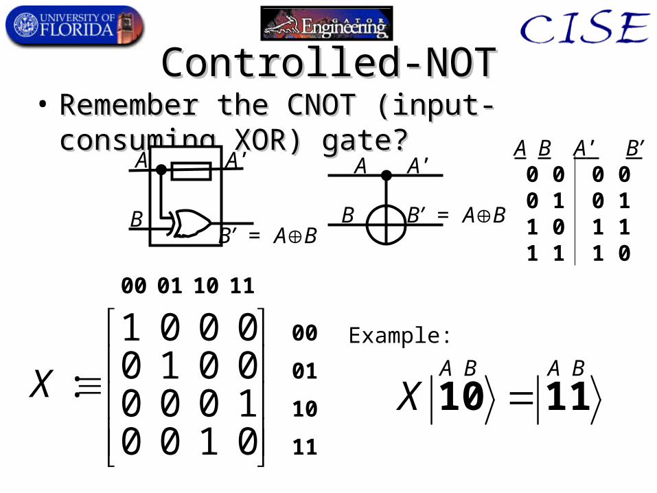
Controlled-NOTControlled-NOT• Remember the CNOT (input-consuming XOR) Remember the CNOT (input-consuming XOR)
gate?gate?A A’
B B’ = AB
A A’
BB’ = AB
A B A’ B’0 0 0 00 1 0 11 0 1 11 1 1 0
11
10
01
00
11100100
0100100000100001
:X 1110 X
Example:
A B A B
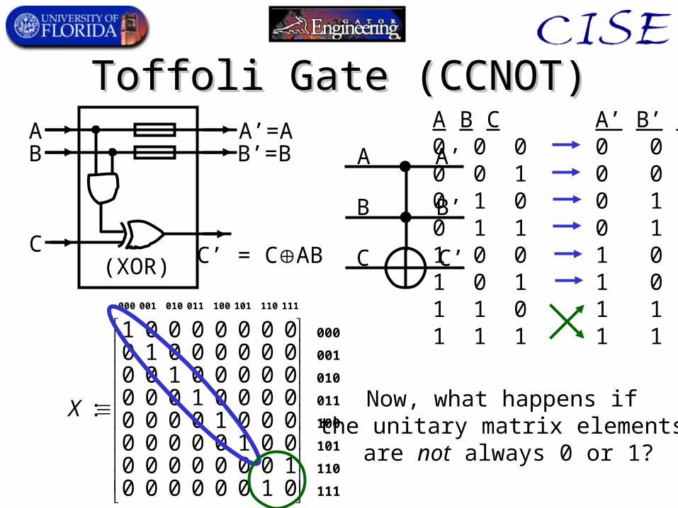
Toffoli Gate (CCNOT)Toffoli Gate (CCNOT)A B C A’ B’ C’0 0 0 0 0 00 0 1 0 0 10 1 0 0 1 00 1 1 0 1 11 0 0 1 0 01 0 1 1 0 11 1 0 1 1 01 1 1 1 1 1
(XOR)
AB
C
A’=AB’=B
C’ = CAB
A
B’B
C
A’
C’
111
110
101
100
011
010
001
000
111110 101100 011010 001000
0100000010000000001000000001000000001000000001000000001000000001
:X Now, what happens if the unitary matrix elements
are not always 0 or 1?
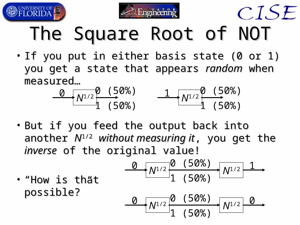
The Square Root of NOTThe Square Root of NOT• If you put in either basis state (0 or 1) you get a state If you put in either basis state (0 or 1) you get a state
that appears that appears randomrandom when measured… when measured…
• But if you feed the output back into another But if you feed the output back into another NN1/21/2 without measuring itwithout measuring it, you get the , you get the inverseinverse of the of the original value!original value!
• ““How is thatHow is thatpossible?”possible?”
N1/20 0 (50%)
1 (50%)N1/21 0 (50%)
1 (50%)
N1/20 0 (50%)
1 (50%)N1/2 1
N1/20 0 (50%)
1 (50%)N1/2 0
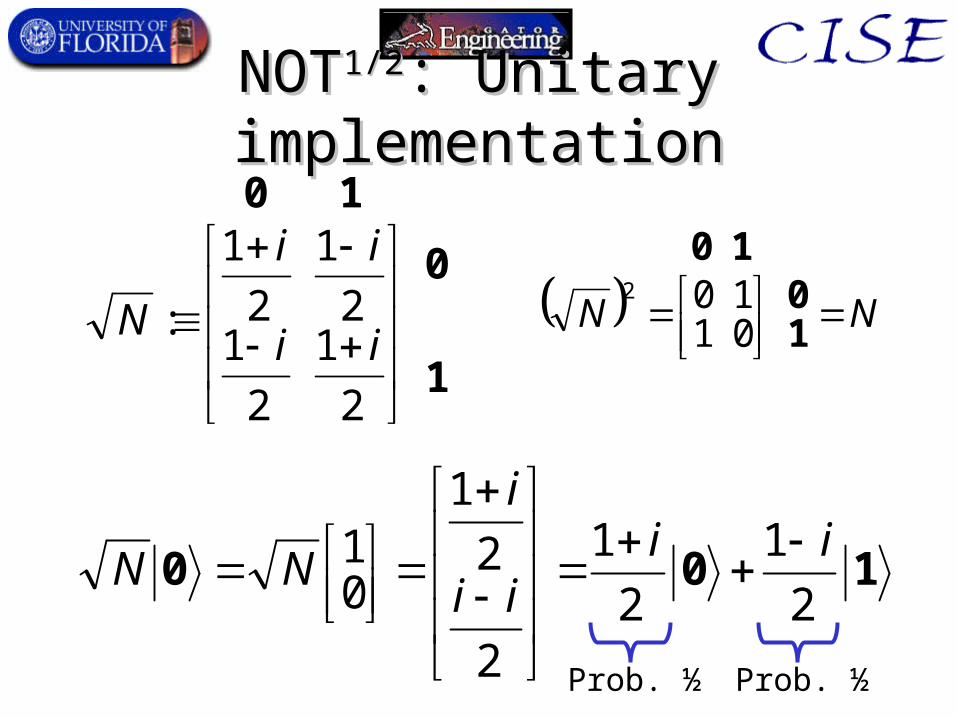
NOTNOT1/21/2: Unitary implementation: Unitary implementation
1
0
1 0
2
1
2
12
1
2
1
:ii
ii
N NN
1
010
01102
1002
1
2
1
2
2
1
01 ii
ii
i
NN
Prob. ½ Prob. ½
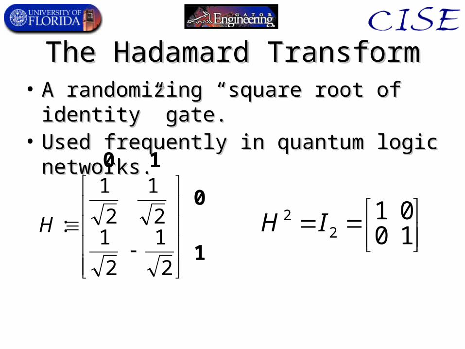
The Hadamard TransformThe Hadamard Transform• A randomizing “square root of identity” gate.A randomizing “square root of identity” gate.• Used frequently in quantum logic networks.Used frequently in quantum logic networks.
1
0
1 0
2
1
2
12
1
2
1
:H
10
012
2 IH
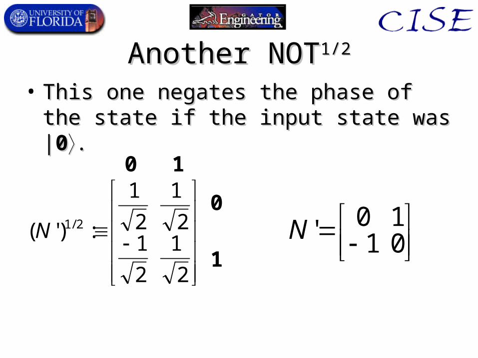
Another NOTAnother NOT1/21/2
• This one negates the phase of the state if the This one negates the phase of the state if the input state was |input state was |00..
1
0
1 0
2
1
2
12
1
2
1
:)'( 2/1N
01
10'N
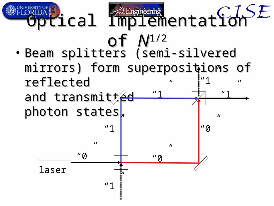
Optical Implementation of Optical Implementation of NN1/21/2
• Beam splitters (semi-silvered mirrors) form Beam splitters (semi-silvered mirrors) form superpositions of reflected superpositions of reflected and transmittedand transmittedphoton states.photon states.
“0”
“1”
“1”
“1”
“0”
“0”
“1”
“1”
laser
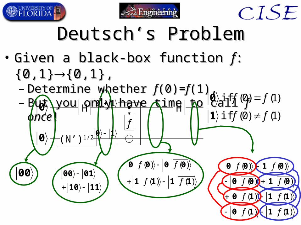
Deutsch’s ProblemDeutsch’s Problem• Given a black-box function Given a black-box function ff:{0,1}:{0,1}{0,1},{0,1},
– Determine whether Determine whether ff(0)=(0)=ff(1),(1),– But you only have time to call But you only have time to call ff onceonce!!
H H
f
0
0 (N’)1/2
10
10
)1()0( if
)1()0( if
ff
ff
1
0
00)()(
)()(
1 11 1
0 00 0
ff
ff
1110
0100
)()(
)()(
)()(
)()(
1 11 0
1 11 0
0 10 0
0 10 0
ff
ff
ff
ff
Extended Deutsch’s ProblemExtended Deutsch’s Problem• Given black-box Given black-box ff:{0,1}:{0,1}nn{0,1},{0,1},
– and a guarantee that and a guarantee that ff is either is either constantconstant or or balancedbalanced (1 on (1 on exactly ½ of inputs)exactly ½ of inputs)
– Which is it?Which is it?– Minimize number of calls to Minimize number of calls to ff..
• Classical algorithm, worst-case:Classical algorithm, worst-case:– Order 2Order 2nn time! time!
• What if the first 2What if the first 2nn−−11 cases examined are all 0? cases examined are all 0?– Function couldFunction could still still be either constant or balanced.be either constant or balanced.
• Case number 2Case number 2nn-1-1+1: if 0, constant; if 1, balanced.+1: if 0, constant; if 1, balanced.
• Quantum algorithm is exponentially faster!Quantum algorithm is exponentially faster!– (Deutsch & Jozsa, 1992.)(Deutsch & Jozsa, 1992.)
Universal Q-Gates: HistoryUniversal Q-Gates: History• Deutsch ‘89:Deutsch ‘89:
– Universal 3-bit Toffoli-like gate.Universal 3-bit Toffoli-like gate.
• diVincenzo ‘95:diVincenzo ‘95:– Adequate set of 2-bit gates.Adequate set of 2-bit gates.
• Barenco ‘95:Barenco ‘95:– Universal 2-bit gate.Universal 2-bit gate.
• Deutsch Deutsch et al.et al. ‘95 ‘95– Almost all 2-bit gates are universal.Almost all 2-bit gates are universal.
• Barenco Barenco et al.et al. ‘95 ‘95– CNOT + set of 1-bit gates is adequate.CNOT + set of 1-bit gates is adequate.
• Later development of discrete gate sets...Later development of discrete gate sets...
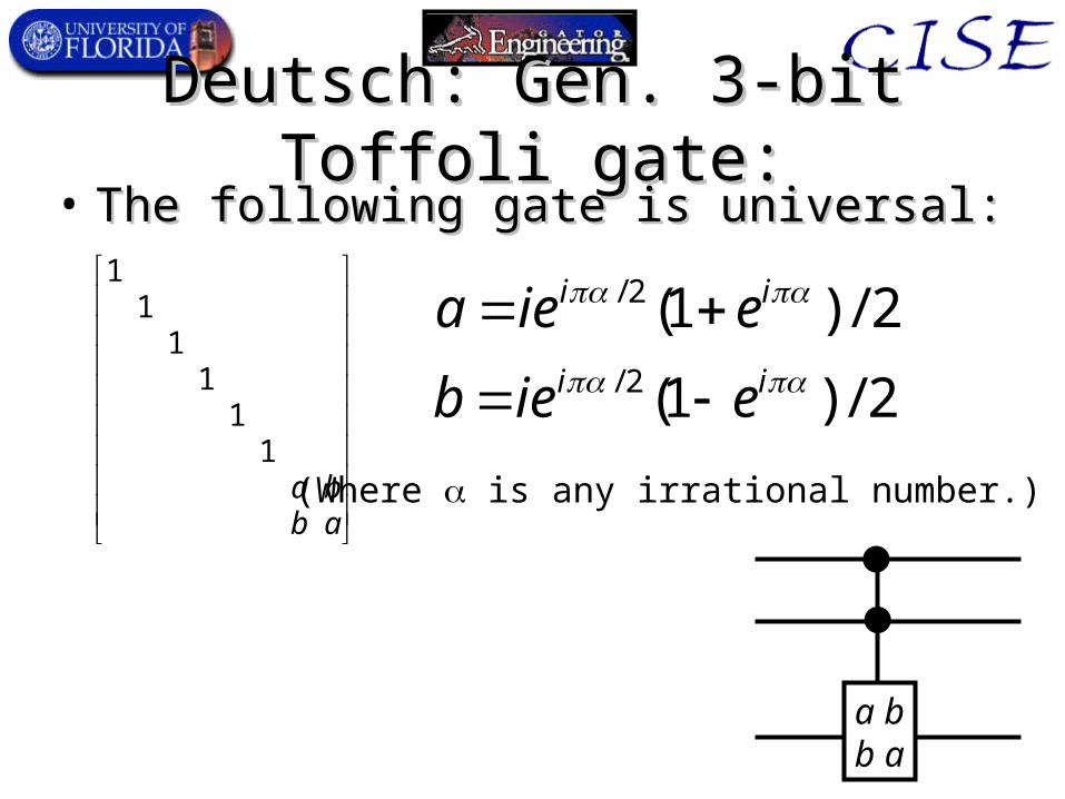
Deutsch: Gen. 3-bit Toffoli gate:Deutsch: Gen. 3-bit Toffoli gate:• The following gate is universal:The following gate is universal:
abba
11
11
11
2/)1(
2/)1(2/
2/
ii
ii
eieb
eiea
a bb a
(Where is any irrational number.)
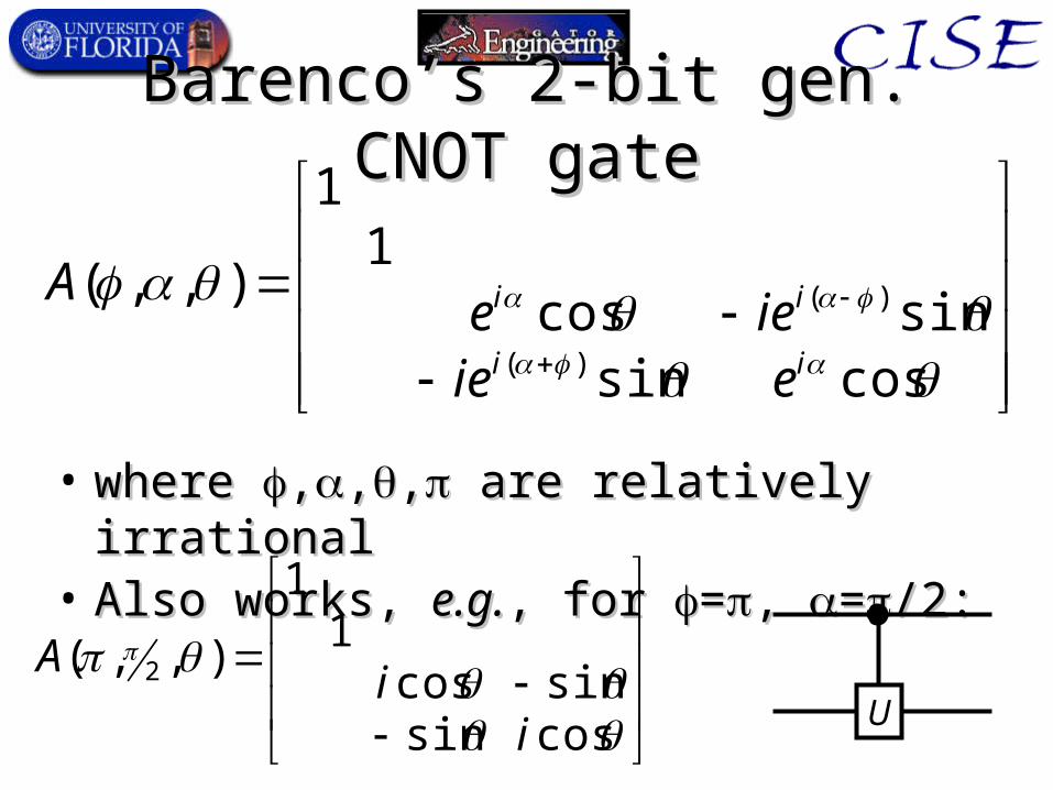
Barenco’s 2-bit gen. CNOT gateBarenco’s 2-bit gen. CNOT gate
• where where ,,,,,, are relatively irrational are relatively irrational• Also works, Also works, e.g.e.g., for , for ==, , ==/2:/2:
cossinsincos
11
),,(
)(
)(
ii
ii
eieiee
A
cossinsincos
11
),,( 2
ii
AU
Barenco Barenco et al.et al. ‘95 results ‘95 results• Universality of CNOT + 1-bit gatesUniversality of CNOT + 1-bit gates
– 2-bit Barenco gate already known universal2-bit Barenco gate already known universal– 4 1-bit gates + 2 CNOTs suffice to build it4 1-bit gates + 2 CNOTs suffice to build it
• Construction of generalized Toffoli gatesConstruction of generalized Toffoli gates– 3-bit version via five 2-bit gates3-bit version via five 2-bit gates– nn-bit version via -bit version via OO((nn22) 2-bit gates) 2-bit gates– No auxilliary bits needed for the aboveNo auxilliary bits needed for the above
• All operations done “in place” on input qubits.All operations done “in place” on input qubits.– nn-bit version via -bit version via OO((nn) 2-bit gates, given 1 work bit) 2-bit gates, given 1 work bit
Quantum Complexity TheoryQuantum Complexity Theory• Early developments:Early developments:
– Deutch’s problem (from earlier): Slight speedupDeutch’s problem (from earlier): Slight speedup– Deutsch & Jozsa: Exponential speed-upDeutsch & Jozsa: Exponential speed-up
• Important quantum complexity classes:Important quantum complexity classes:– EQPEQP: Exact Quantum Polynomial - like : Exact Quantum Polynomial - like PP..
• Polynomial time, deterministic.Polynomial time, deterministic.– ZQPZQP: Zero-error Quantum Polynomial - like : Zero-error Quantum Polynomial - like ZPPZPP..
• Probabilistic, expected polynomial-time, zero errors.Probabilistic, expected polynomial-time, zero errors.– BQPBQP: Bounded-error Quantum Poly. - like : Bounded-error Quantum Poly. - like BPPBPP..
• Probabilistic, bounded probability of errors.Probabilistic, bounded probability of errors.
• All results relativized, All results relativized, e.g.e.g.,, OO: : EQPEQPOO ( (NPNPO O co-NPco-NPOO)) Given a certain black-box, quantum
computers can solve a certain problemfaster than a classical computer can
even check the answer!

Quantum AlgorithmsQuantum Algorithms
Part I: Unstructured SearchPart I: Unstructured Search
Unstructured Search ProblemUnstructured Search Problem• Given a set Given a set SS of of NN elements and a black-box function elements and a black-box function
ff::SS{0,1}, find an element {0,1}, find an element xxSS such that such that ff((xx)=1, if )=1, if one exists (or if not, say so).one exists (or if not, say so).– Any NP problem can be cast as an unstructured search Any NP problem can be cast as an unstructured search
problem.problem.• Not necessarily the optimal approach, however.Not necessarily the optimal approach, however.
• Bounds on classical run-time:Bounds on classical run-time: ((NN) expected queries in worst case (0 or 1 sol’ns):) expected queries in worst case (0 or 1 sol’ns):
• Have to try Have to try NN/2 elements on average before finding sol’n./2 elements on average before finding sol’n.• Have to try all Have to try all NN if there is no solution. if there is no solution.
• If elements are length-If elements are length- bit strings, bit strings,– Expected #trials is Expected #trials is (2(2) - exponential in ) - exponential in . Bad!. Bad!
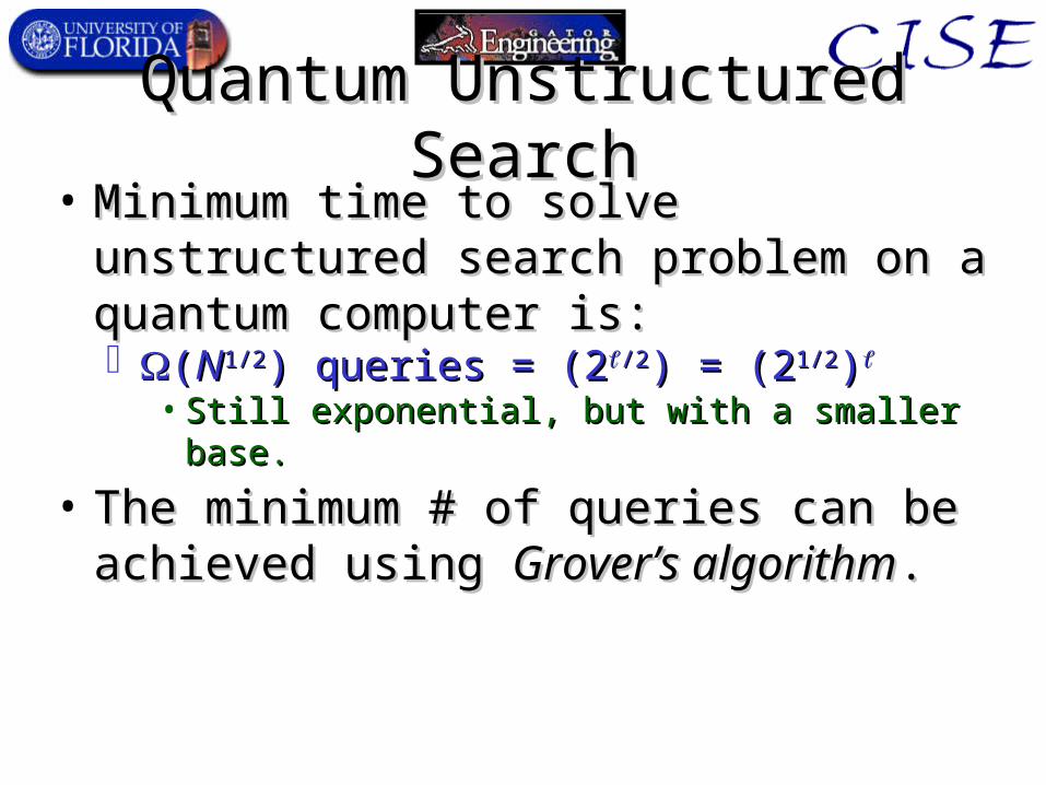
Quantum Unstructured SearchQuantum Unstructured Search• Minimum time to solve unstructured search Minimum time to solve unstructured search
problem on a quantum computer is:problem on a quantum computer is: ((NN1/21/2) queries = (2) queries = (2/2/2) = (2) = (21/21/2))
• Still exponential, but with a smaller base.Still exponential, but with a smaller base.
• The minimum # of queries can be achieved The minimum # of queries can be achieved using using Grover’s algorithmGrover’s algorithm..
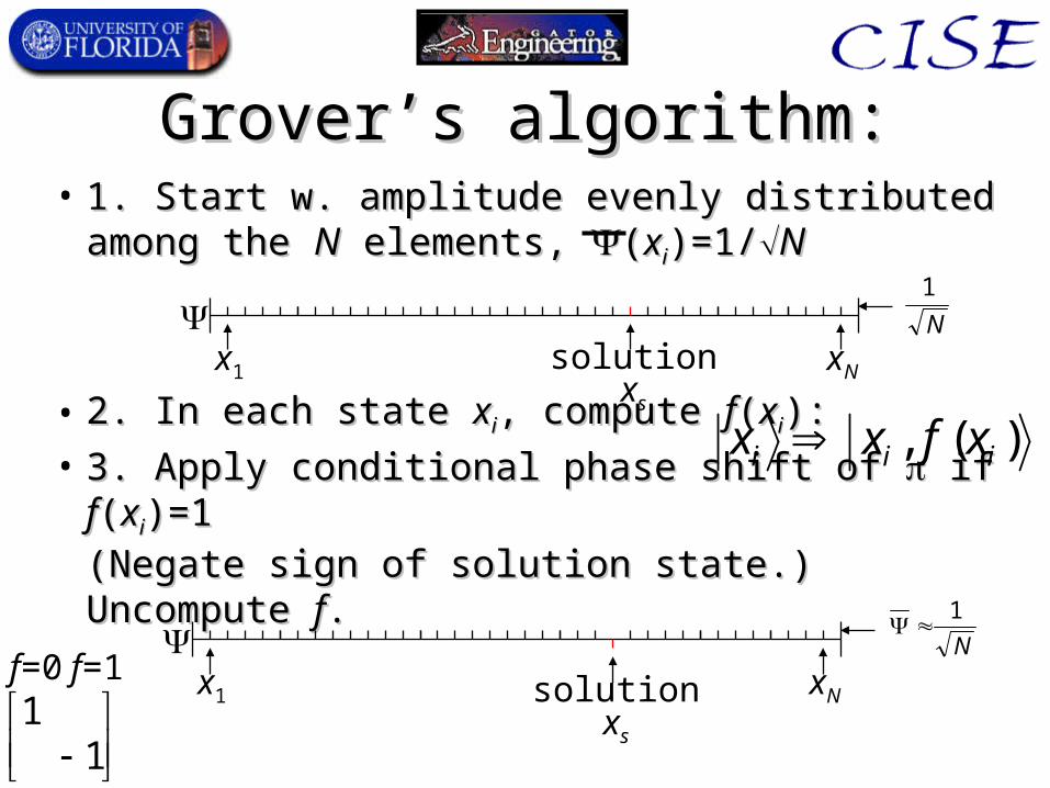
Grover’s algorithm:Grover’s algorithm:• 1. Start w. amplitude evenly distributed among 1. Start w. amplitude evenly distributed among
the the NN elements, elements, ((xxii)=1/)=1/NN
• 2. In each state 2. In each state xxii, compute , compute ff((xxii):):
• 3. Apply conditional phase shift of 3. Apply conditional phase shift of if if ff((xxii)=1)=1
(Negate sign of solution state.) Uncompute (Negate sign of solution state.) Uncompute ff..
N
1
x1 xNsolutionxs
)(, iii xfxx
N
1
x1 xNsolutionxs
1
1f=0 f=1
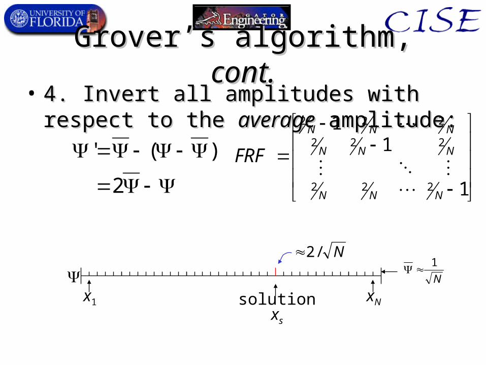
Grover’s algorithm, Grover’s algorithm, cont.cont.• 4. Invert all amplitudes with respect to the 4. Invert all amplitudes with respect to the
averageaverage amplitude: amplitude:
2
)('
1
11
222
222
222
NNN
NNN
NNN
FRF
N
1
x1 xNsolutionxs
N/2
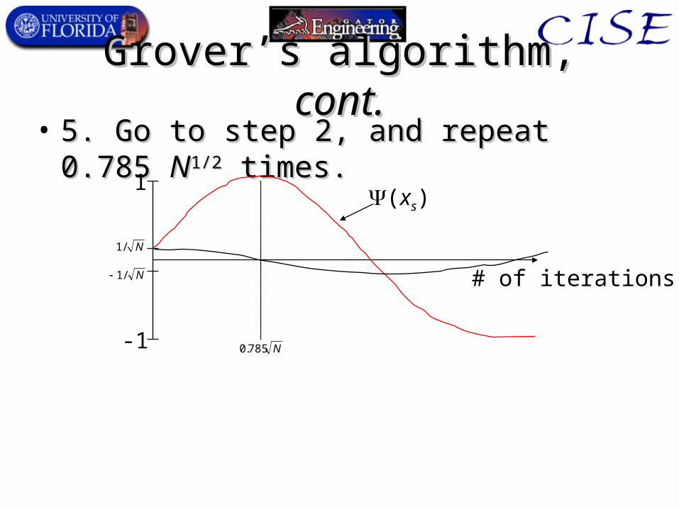
Grover’s algorithm, Grover’s algorithm, cont.cont.• 5. Go to step 2, and repeat 0.785 5. Go to step 2, and repeat 0.785 NN1/21/2 times. times.
1
-1
N/1
N/1
N785.0
# of iterations
(xs)
Shor’s Factoring AlgorithmShor’s Factoring Algorithm• Solves the >2000-year-old problem:Solves the >2000-year-old problem:
– Given a large number Given a large number NN, quickly find the prime , quickly find the prime factorization of factorization of NN. (At least as old as Euclid!). (At least as old as Euclid!)
• No polynomial-time (as a function of No polynomial-time (as a function of nn=lg =lg NN) ) classical algorithm for this problem is known.classical algorithm for this problem is known.– The best known (as of 1993) was a The best known (as of 1993) was a number field sievenumber field sieve
algorithm taking time algorithm taking time OO(exp((exp(nn1/3 1/3 log(log(nn2/32/3))))))– However, there is also no proof that an (undis-covered) However, there is also no proof that an (undis-covered)
fast classical algorithm does fast classical algorithm does notnot exist. exist.
• Shor’s quantum algorithm takes time Shor’s quantum algorithm takes time OO((nn22))– No worse than multiplication of No worse than multiplication of nn-bit numbers!-bit numbers!
Elements of Shor’s AlgorithmElements of Shor’s Algorithm• Uses a standard reduction of factoring to another Uses a standard reduction of factoring to another
number-theory problem called the number-theory problem called the discrete logarithmdiscrete logarithm problem.problem.
• The discrete logarithm problem corresponds to The discrete logarithm problem corresponds to finding the finding the periodperiod of a certain periodic function of a certain periodic function defined over the integers.defined over the integers.
• A general way to find the period of a function is to A general way to find the period of a function is to perform a perform a Fourier transformFourier transform on the function. on the function.– Shor showed how to generalize an earlier algorithm by Shor showed how to generalize an earlier algorithm by
Simon, to provide a Quantum Fourier Transform that is Simon, to provide a Quantum Fourier Transform that is exponentially faster than classical ones.exponentially faster than classical ones.
Powers of numbers mod Powers of numbers mod NN• Given natural numbers (non-negative integers) Given natural numbers (non-negative integers) NN1, 1,
xx<<NN, and , and xx, consider the sequence:, consider the sequence:xx00 mod mod NN, , xx11 mod mod NN, , xx22 mod mod NN, … , … = 1, = 1, xx, , xx22 mod mod NN, …, …
• If If xx and and NN are relatively prime, this sequence is are relatively prime, this sequence is guaranteed not to repeat until it gets back to 1.guaranteed not to repeat until it gets back to 1.
• Discrete logarithmDiscrete logarithm of of yy, base , base xx, mod , mod NN: : – The smallest natural number exponent The smallest natural number exponent kk (if any) such that (if any) such that
xxkk = = yy (mod (mod NN).).– I.e.I.e., the integer logarithm of , the integer logarithm of yy, base , base xx, in modulo-, in modulo-NN
arithmetic. Example: dlogarithmetic. Example: dlog77 13 (mod 13 (mod NN) = ?) = ?
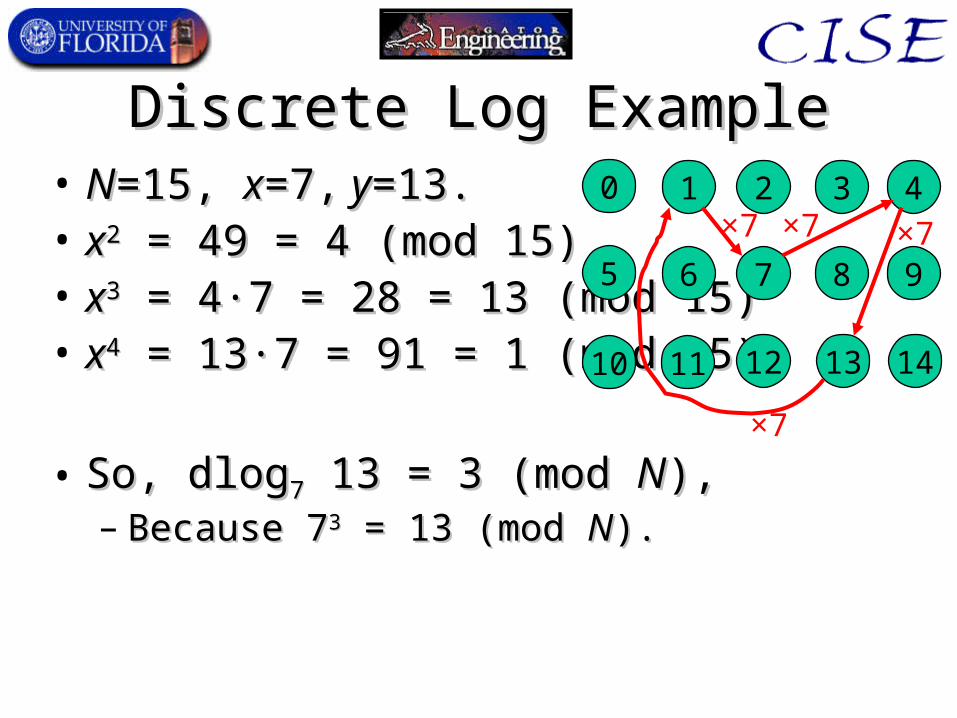
Discrete Log ExampleDiscrete Log Example• NN=15, =15, xx=7,=7, y y=13.=13.• xx22 = 49 = 4 (mod 15) = 49 = 4 (mod 15)• xx33 = 4·7 = 28 = 13 (mod 15) = 4·7 = 28 = 13 (mod 15)• xx44 = 13·7 = 91 = 1 (mod 15) = 13·7 = 91 = 1 (mod 15)
• So, dlogSo, dlog77 13 = 3 (mod 13 = 3 (mod NN),),– Because 7Because 733 = 13 (mod = 13 (mod NN).).
0 1 2 3 4
5 6 7 8 9
10 11 12 13 14
×7 ×7 ×7
×7
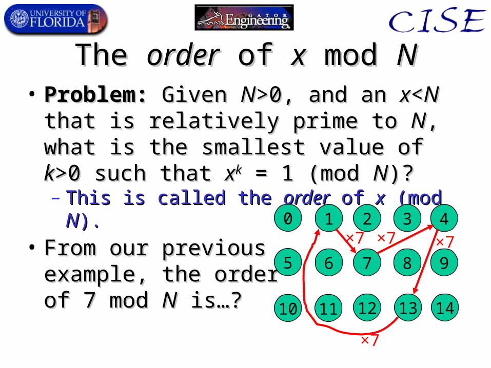
The The orderorder of of xx mod mod NN• Problem:Problem: Given Given NN>0, and an >0, and an xx<<NN that is that is
relatively prime to relatively prime to NN, what is the smallest value , what is the smallest value of of kk>0 such that >0 such that xxkk = 1 (mod = 1 (mod NN)?)?– This is called the This is called the orderorder of of xx (mod (mod NN).).
• From our previousFrom our previousexample, the orderexample, the orderof 7 mod of 7 mod NN is…? is…?
0 1 2 3 4
5 6 7 8 9
10 11 12 13 14
×7 ×7 ×7
×7
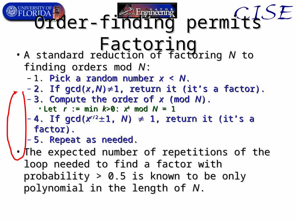
Order-finding permits FactoringOrder-finding permits Factoring• A standard reduction of factoring A standard reduction of factoring NN to finding orders to finding orders
mod mod NN::– 1. 1. Pick a random number Pick a random number xx < < NN..– 2. If gcd(2. If gcd(xx,,NN))1, return it (it’s a factor).1, return it (it’s a factor).– 3. Compute the order of 3. Compute the order of xx (mod (mod NN).).
• Let Let r r := min := min kk>0: >0: xxkk mod mod NN = 1 = 1– 4. If gcd(4. If gcd(xxrr/2/21, 1, NN) ) 1, return it (it’s a factor). 1, return it (it’s a factor).– 5. Repeat as needed.5. Repeat as needed.
• The expected number of repetitions of the loop The expected number of repetitions of the loop needed to find a factor with probability > 0.5 is needed to find a factor with probability > 0.5 is known to be only polynomial in the length of known to be only polynomial in the length of NN. .
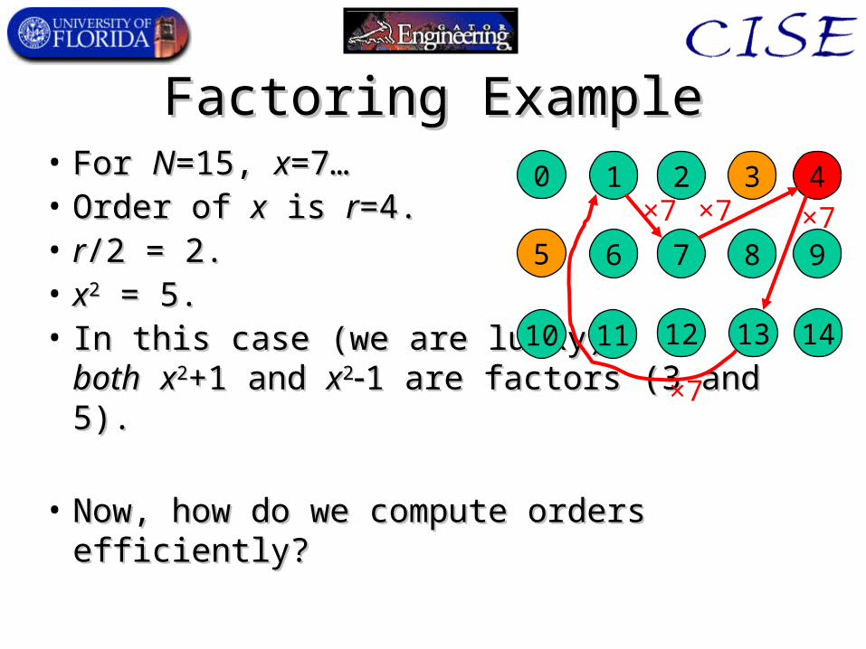
Factoring ExampleFactoring Example• For For NN=15, =15, xx=7…=7…• Order of Order of xx is is rr=4.=4.• rr/2 = 2./2 = 2.• xx22 = 5. = 5.• In this case (we are lucky), In this case (we are lucky),
bothboth xx22+1 and +1 and xx221 are factors (3 and 5).1 are factors (3 and 5).
• Now, how do we compute orders efficiently?Now, how do we compute orders efficiently?
0 1 2 3 4
5 6 7 8 9
10 11 12 13 14
×7 ×7 ×7
×7
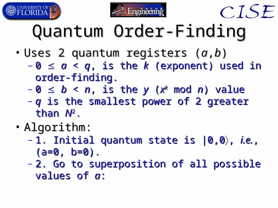
Quantum Order-FindingQuantum Order-Finding• Uses 2 quantum registers (Uses 2 quantum registers (aa,,bb))
– 0 0 aa < < qq, is the , is the kk (exponent) used in order-finding. (exponent) used in order-finding.– 0 0 bb < < nn, is the , is the yy ( (xxkk mod mod nn) value) value– qq is the smallest power of 2 greater than is the smallest power of 2 greater than NN22..
• Algorithm:Algorithm:– 1. Initial quantum state is |0,01. Initial quantum state is |0,0, , i.e.i.e., (a=0, b=0)., (a=0, b=0).– 2. Go to superposition of all possible values of 2. Go to superposition of all possible values of aa::
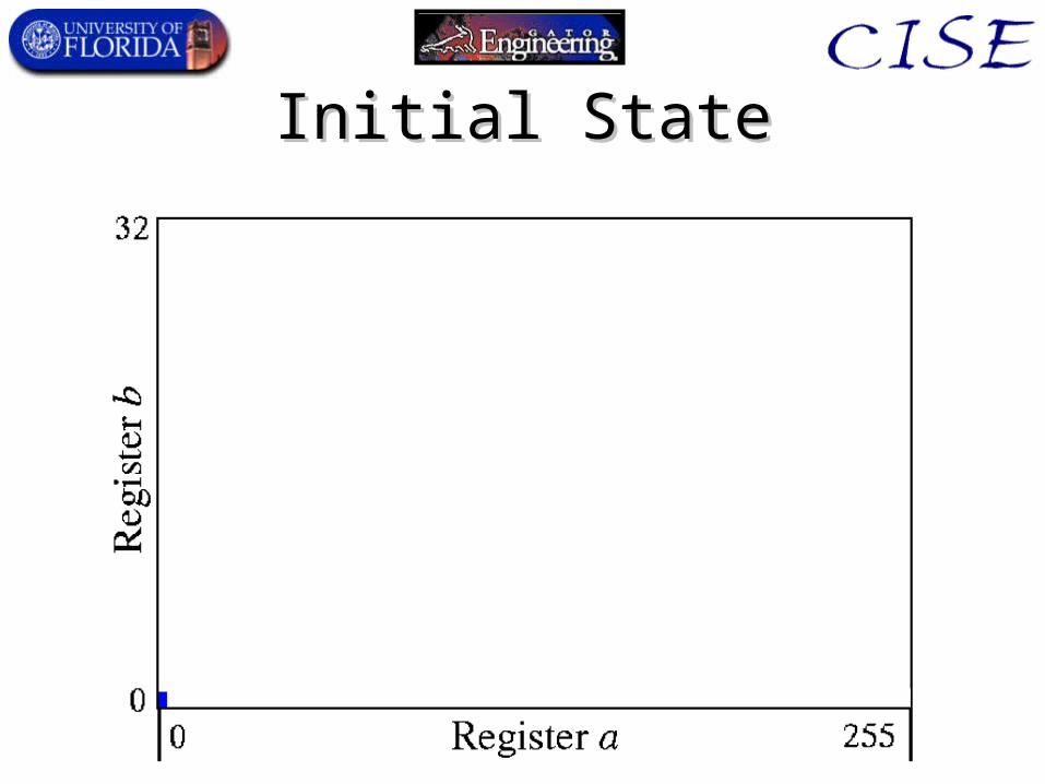
Initial StateInitial State
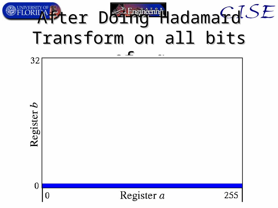
After Doing Hadamard After Doing Hadamard Transform on all bits of Transform on all bits of aa
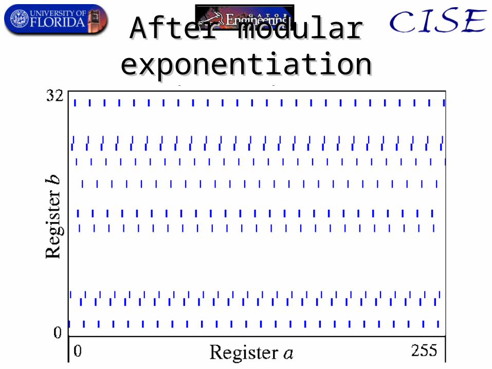
After modular exponentiationAfter modular exponentiationbb==xxaa (mod (mod NN))
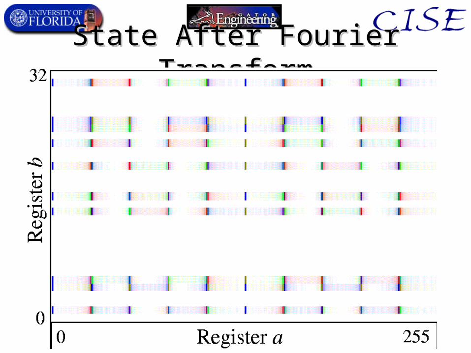
State After Fourier TransformState After Fourier Transform
Quantum Algorithms IIIQuantum Algorithms III
Wrap-up:Wrap-up:Classical vs. Quantum ParallelismClassical vs. Quantum Parallelism
Quantum Physics SimulationsQuantum Physics Simulations
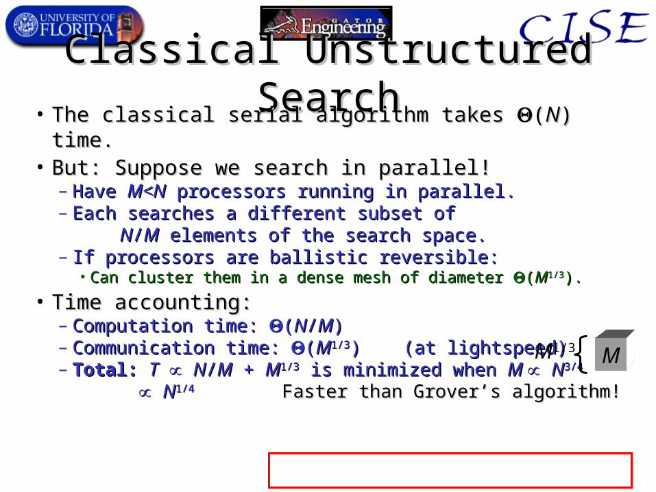
Classical Unstructured SearchClassical Unstructured Search• The classical serial algorithm takes The classical serial algorithm takes ((NN) time.) time.• But: Suppose we search in parallel!But: Suppose we search in parallel!
– Have Have M<NM<N processors running in parallel. processors running in parallel.– Each searches a different subset ofEach searches a different subset of
NN//MM elements of the search space. elements of the search space.– If processors are ballistic reversible:If processors are ballistic reversible:
• Can cluster them in a dense mesh of diameter Can cluster them in a dense mesh of diameter ((MM1/31/3).).
• Time accounting:Time accounting:– Computation time: Computation time: ((NN//MM))– Communication time: Communication time: ((MM1/31/3)) (at lightspeed)(at lightspeed)– Total:Total: TT NN//MM + + MM1/31/3 is minimized when is minimized when M M NN3/43/4
NN1/41/4 Faster than Grover’s algorithm! Faster than Grover’s algorithm!
MM1/3
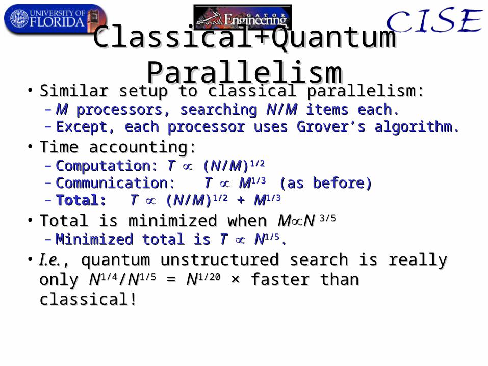
Classical+Quantum ParallelismClassical+Quantum Parallelism• Similar setup to classical parallelism: Similar setup to classical parallelism:
– MM processors, searching processors, searching NN//MM items each. items each.– Except, each processor uses Grover’s algorithm.Except, each processor uses Grover’s algorithm.
• Time accounting:Time accounting:– Computation:Computation: TT ( (NN//MM))1/21/2
– Communication:Communication: TT MM1/31/3 (as before)(as before)– Total:Total: TT ( (NN//MM))1/21/2 + + MM1/31/3
• Total is minimized when Total is minimized when MMN N 3/53/5
– Minimized total is Minimized total is TT NN1/51/5..
• I.e.I.e., quantum unstructured search is really only , quantum unstructured search is really only NN1/41/4//NN1/51/5 = = NN1/201/20 × faster than classical! × faster than classical!

Simulating Quantum PhysicsSimulating Quantum Physics• For For nn particles, takes exponential time using the particles, takes exponential time using the
best known classical methods.best known classical methods.– Feynman suggested: use quantum computingFeynman suggested: use quantum computing
• Takes only polynomial time on a QC.Takes only polynomial time on a QC.• History of some fast QC physics algorithms:History of some fast QC physics algorithms:
– Schrödinger equation (Boghosian, Yepez)Schrödinger equation (Boghosian, Yepez)– Many-body Fermi systems (Abrams & Lloyd)Many-body Fermi systems (Abrams & Lloyd)– Eigenvalue/eigenvector computations (ditto)Eigenvalue/eigenvector computations (ditto)– Quantum lattice gases, Ising models, Quantum lattice gases, Ising models, etc.etc.– Totally general quantum physics simulationsTotally general quantum physics simulations
(Field theories, etc.) - Lloyd 1996(Field theories, etc.) - Lloyd 1996
Simulating Quantum ComputersSimulating Quantum Computers
on classical oneson classical ones
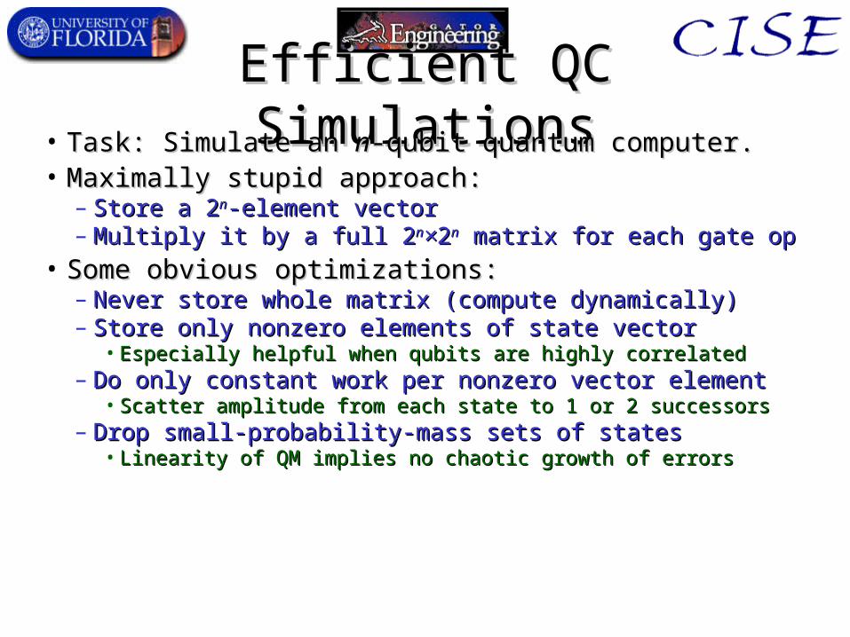
Efficient QC SimulationsEfficient QC Simulations• Task: Simulate an Task: Simulate an nn-qubit quantum computer.-qubit quantum computer.• Maximally stupid approach:Maximally stupid approach:
– Store a 2Store a 2nn-element vector-element vector– Multiply it by a full 2Multiply it by a full 2nn××22nn matrix for each gate op matrix for each gate op
• Some obvious optimizations:Some obvious optimizations:– Never store whole matrix (compute dynamically)Never store whole matrix (compute dynamically)– Store only nonzero elements of state vectorStore only nonzero elements of state vector
• Especially helpful when qubits are highly correlatedEspecially helpful when qubits are highly correlated– Do only constant work per nonzero vector elementDo only constant work per nonzero vector element
• Scatter amplitude from each state to 1 or 2 successorsScatter amplitude from each state to 1 or 2 successors– Drop small-probability-mass sets of statesDrop small-probability-mass sets of states
• Linearity of QM implies no chaotic growth of errorsLinearity of QM implies no chaotic growth of errors
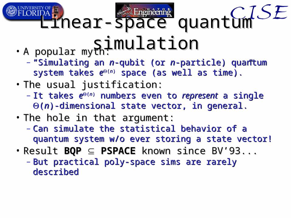
Linear-space quantum simulationLinear-space quantum simulation• A popular myth:A popular myth:
– ““Simulating an Simulating an nn-qubit (or -qubit (or nn-particle) quantum system -particle) quantum system takes takes ee((nn)) space (as well as time).” space (as well as time).”
• The usual justification:The usual justification:– It takes It takes ee((nn)) numbers even to numbers even to representrepresent a single a single ((nn)-)-
dimensional state vector, in general.dimensional state vector, in general.
• The hole in that argument:The hole in that argument:– Can simulate the statistical behavior of a quantum system Can simulate the statistical behavior of a quantum system
w/o ever storing a state vector!w/o ever storing a state vector!
• Result Result BQPBQP PSPACEPSPACE known since BV’93... known since BV’93...– But practical poly-space sims are rarely describedBut practical poly-space sims are rarely described
The Basic IdeaThe Basic Idea• Inspiration:Inspiration:
– Feynman’s Feynman’s path integralpath integral formulation of QED. formulation of QED.– Gives the amplitude of a given final configuration Gives the amplitude of a given final configuration
by accumulating amplitude over all paths from by accumulating amplitude over all paths from initial to final configurations.initial to final configurations.
– Each path consists of only a single Each path consists of only a single ((nn)-coordinate )-coordinate configuration at each time, configuration at each time, notnot a full wavefunction a full wavefunction over the configuration space.over the configuration space.
– Can enumerate all paths, Can enumerate all paths, while only ever while only ever representing one path at a time.representing one path at a time.
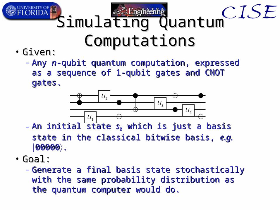
Simulating Quantum ComputationsSimulating Quantum Computations• Given:Given:
– Any Any nn-qubit quantum computation, expressed as a -qubit quantum computation, expressed as a sequence of 1-qubit gates and CNOT gates.sequence of 1-qubit gates and CNOT gates.
– An initial state An initial state ss00 which is just a basis state in the which is just a basis state in the
classical bitwise basis, classical bitwise basis, e.g.e.g. 0000000000..• Goal:Goal:
– Generate a final basis state stochastically with the Generate a final basis state stochastically with the same probability distribution as the quantum same probability distribution as the quantum computer would do.computer would do.
U1
U3
U4
U2
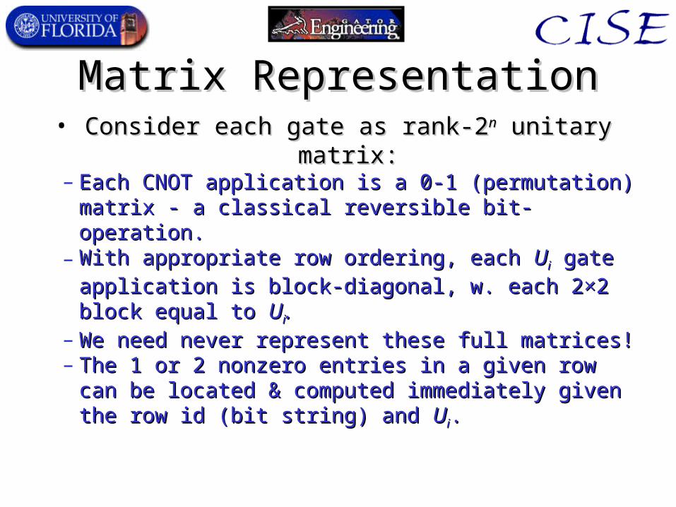
Matrix RepresentationMatrix Representation• Consider each gate as rank-2Consider each gate as rank-2nn unitary matrix: unitary matrix:
– Each CNOT application is a 0-1 (permutation) Each CNOT application is a 0-1 (permutation) matrix - a classical reversible bit-operation.matrix - a classical reversible bit-operation.
– With appropriate row ordering, each With appropriate row ordering, each UUii gate gate
application is block-diagonal, w. each 2×2 block application is block-diagonal, w. each 2×2 block equal to equal to UUii..
– We need never represent these full matrices!We need never represent these full matrices!– The 1 or 2 nonzero entries in a given row can be The 1 or 2 nonzero entries in a given row can be
located & computed immediately given the row id located & computed immediately given the row id (bit string) and (bit string) and UUii..
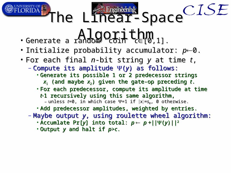
The Linear-Space AlgorithmThe Linear-Space Algorithm• Generate a random “coin” Generate a random “coin” cc[0,1]. [0,1]. • Initialize probability accumulator: Initialize probability accumulator: pp0.0.• For each final For each final nn-bit string -bit string yy at time at time tt,,
– Compute its amplitude Compute its amplitude ((yy) as follows:) as follows:• Generate its possible 1 or 2 predecessor stringsGenerate its possible 1 or 2 predecessor strings
xx11 (and maybe (and maybe xx22) given the gate-op preceding ) given the gate-op preceding tt..• For each predecessor, compute its amplitude at time For each predecessor, compute its amplitude at time tt1 1
recursively using this same algorithm,recursively using this same algorithm,– unless unless tt=0, in which case =0, in which case =1 if =1 if xx==ss00, 0 otherwise., 0 otherwise.
• Add predecessor amplitudes, weighted by entries.Add predecessor amplitudes, weighted by entries.– Maybe output Maybe output yy, using roulette wheel algorithm:, using roulette wheel algorithm:
• Accumlate Pr[Accumlate Pr[yy] into total: ] into total: p p p +||p +||((yy)||)||22
• Output Output yy and halt if and halt if pp>>cc..
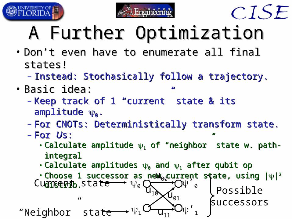
A Further OptimizationA Further Optimization• Don’t even have to enumerate all final states!Don’t even have to enumerate all final states!
– Instead: Stochasically follow a trajectory.Instead: Stochasically follow a trajectory.
• Basic idea:Basic idea:– Keep track of 1 “current” state & its amplitude Keep track of 1 “current” state & its amplitude 00..– For CNOTs: Deterministically transform state.For CNOTs: Deterministically transform state.– For For UUs:s:
• Calculate amplitude Calculate amplitude 11 of “neighbor” state w. path-integral of “neighbor” state w. path-integral• Calculate amplitudes Calculate amplitudes 00 and and 11 after qubit op after qubit op• Choose 1 successor as new current state, using |Choose 1 successor as new current state, using |||22 distrib. distrib.
0
1
u00
u10 u01
u11
’0
’1
Possiblesuccessors
Current state
“Neighbor” state
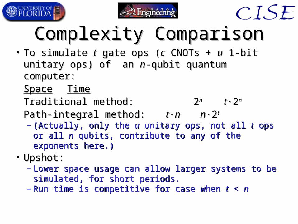
Complexity ComparisonComplexity Comparison• To simulate To simulate tt gate ops ( gate ops (cc CNOTs + CNOTs + uu 1-bit unitary 1-bit unitary
ops) of an ops) of an nn-qubit quantum computer:-qubit quantum computer:SpaceSpace TimeTime
Traditional method:Traditional method: 2 2nn tt·2·2nn
Path-integral method:Path-integral method: tt··nn n n·2·2tt
– (Actually, only the (Actually, only the uu unitary ops, not all unitary ops, not all tt ops ops or all or all nn qubits, contribute to any of the exponents here.)qubits, contribute to any of the exponents here.)
• Upshot:Upshot:– Lower space usage can allow larger systems to be Lower space usage can allow larger systems to be
simulated, for short periods.simulated, for short periods.– Run time is competitive for case when Run time is competitive for case when tt < < nn
Quantum Information & Quantum Information & CommunicationCommunication
DecoherenceDecoherenceQuantum Error CorrectionQuantum Error Correction
Quantum CryptographyQuantum Cryptography
DecoherenceDecoherence• The effect that makes macroscopic quantum systems The effect that makes macroscopic quantum systems
appearappear to behave “classically.” to behave “classically.”– Theory was developed in many papers by Zurek.Theory was developed in many papers by Zurek.
• Occurs due to inevitable interactions between a given Occurs due to inevitable interactions between a given quantum system & an unknown (high-entropy) quantum system & an unknown (high-entropy) environment.environment.– Interaction increases (von Neumann-) entropy of the Interaction increases (von Neumann-) entropy of the
reduced density matrix of the quantum system.reduced density matrix of the quantum system.
• Quantum state gradually “collapses” or “decays” to a Quantum state gradually “collapses” or “decays” to a classical statistical mixture of the pointer states classical statistical mixture of the pointer states (measurement eigenstates).(measurement eigenstates).
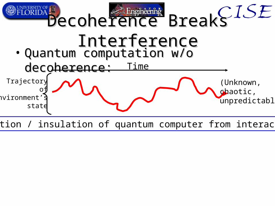
Decoherence Breaks InterferenceDecoherence Breaks Interference• Quantum computation w/o decoherence:Quantum computation w/o decoherence:
Time
Trajectoryof
environment’sstate
(Unknown,chaotic,unpredictable)
Isolation / insulation of quantum computer from interactions
Quantum Information & Quantum Information & Communication Communication cont.cont.
Quantum CryptographyQuantum Cryptography
The The Key Distribution ProblemKey Distribution Problem• How can parties How can parties AA and and BB use a use a physicallyphysically
insecure long-distance communications channel insecure long-distance communications channel to nevertheless to nevertheless securelysecurely exchange keys that exchange keys that they can use to enable future they can use to enable future securesecure, encrypted , encrypted communication between them?communication between them?
• Present-day solution: Present-day solution: Public-Key CryptographyPublic-Key Cryptography– see next slidesee next slide
Public-Key CryptographyPublic-Key Cryptography• AA and and BB each prepare a pair of a each prepare a pair of a public keypublic key and a and a
corresponding corresponding private keyprivate key..– Infeasible to compute private key from public one.Infeasible to compute private key from public one.
• They openly publish their public keys.They openly publish their public keys.• Anyone can now use the public key to encrypt Anyone can now use the public key to encrypt
messages to messages to AA or or BB..– But only the one w. the matching private key can decrypt But only the one w. the matching private key can decrypt
the message.the message.
• Security of technique depends on existence of Security of technique depends on existence of one-one-wayway (a.k.a. (a.k.a. trapdoortrapdoor) functions.) functions. functions believed (but unproven) to be such.functions believed (but unproven) to be such.
PK Crypto vs. Q-ComputingPK Crypto vs. Q-Computing• A serious weakness in most present-day PK A serious weakness in most present-day PK
cryptosystems (such as RSA):cryptosystems (such as RSA):– They depend for their security on the “one-way-ness” of They depend for their security on the “one-way-ness” of
certain functions that is due to the hardness of the certain functions that is due to the hardness of the factoringfactoring and and discrete logarithmdiscrete logarithm problems. problems.
– But, Shor’s algorithm gives a fast way to solve these But, Shor’s algorithm gives a fast way to solve these problems if we just had a quantum computer!problems if we just had a quantum computer!
• Large QCs may be implemented within next 10-20 years.Large QCs may be implemented within next 10-20 years.
• Therefore, data encrypted Therefore, data encrypted todaytoday with these with these cryptosystems cryptosystems cannotcannot be considered secure over multi- be considered secure over multi-decade time-frames!decade time-frames!– But, other PK systems w/o this weakness may exist.But, other PK systems w/o this weakness may exist.

Q-Cryptography to the Rescue!Q-Cryptography to the Rescue!• Features:Features:
– Provides for secure key exchange over physically Provides for secure key exchange over physically unprotected channels w. a unprotected channels w. a guarantee of detectionguarantee of detection of of any eavesdropping of the key.any eavesdropping of the key.
• Doesn’t protect against denial-of-service attacks.Doesn’t protect against denial-of-service attacks.– Physically impossiblePhysically impossible to compromise security to compromise security
(except @ endpoints) barring overthrow of physics!(except @ endpoints) barring overthrow of physics!• Provably secure under known lawsProvably secure under known laws
– Experimentally verifiedExperimentally verified to work perfectly over >48 to work perfectly over >48 km distances (so far) (Hughes ‘99) via fiber-optic km distances (so far) (Hughes ‘99) via fiber-optic networks.networks.
The One-Time PadThe One-Time Pad• The only known The only known provably secureprovably secure cryptosystem. cryptosystem.• Based on a key of the same length as the data to be Based on a key of the same length as the data to be
encrypted.encrypted.– A given key can only be used A given key can only be used once.once.
• The key is simply a random string of bits.The key is simply a random string of bits.• The plaintext is bitwise-XORed with the key to The plaintext is bitwise-XORed with the key to
produce ciphertext.produce ciphertext.• Provably secure because Provably secure because anyany plaintext is equally plaintext is equally
likely to produce the same ciphertext.likely to produce the same ciphertext.• The only problem: How to send the key?The only problem: How to send the key?
Outline of QC Protocol (BB84)Outline of QC Protocol (BB84)• AA chooses a random bit-string chooses a random bit-string
– A key for later use as a one-time pad.A key for later use as a one-time pad.
• AA sends each bit as a qubits with a randomly- sends each bit as a qubits with a randomly-chosen basis (out of 2 different bases).chosen basis (out of 2 different bases).
• BB measures each bit in a randomly-chosen basis measures each bit in a randomly-chosen basis (out of the same 2 bases).(out of the same 2 bases).
• AA & & BB publicly determine which bits they chose the publicly determine which bits they chose the same bases for.same bases for.
• They publicly spot-check a random subset of the They publicly spot-check a random subset of the bits for errors, and use remaining bits.bits for errors, and use remaining bits.
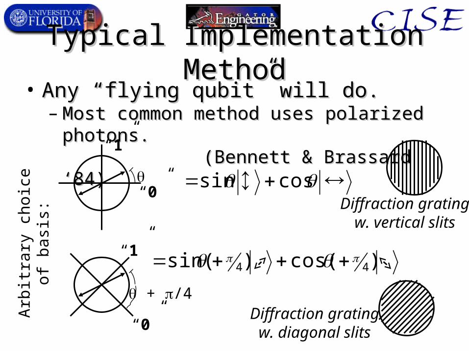
Typical Implementation MethodTypical Implementation Method• Any “flying qubit” will do.Any “flying qubit” will do.
– Most common method uses polarized photons.Most common method uses polarized photons.(Bennett & Brassard ‘84)(Bennett & Brassard ‘84)
Arb
itra
ry c
hoic
eof
bas
is:
“0”
“1”
cossin Diffraction grating
w. vertical slits
+ /4
“0”
“1” )cos( )sin( 44
Diffraction gratingw. diagonal slits
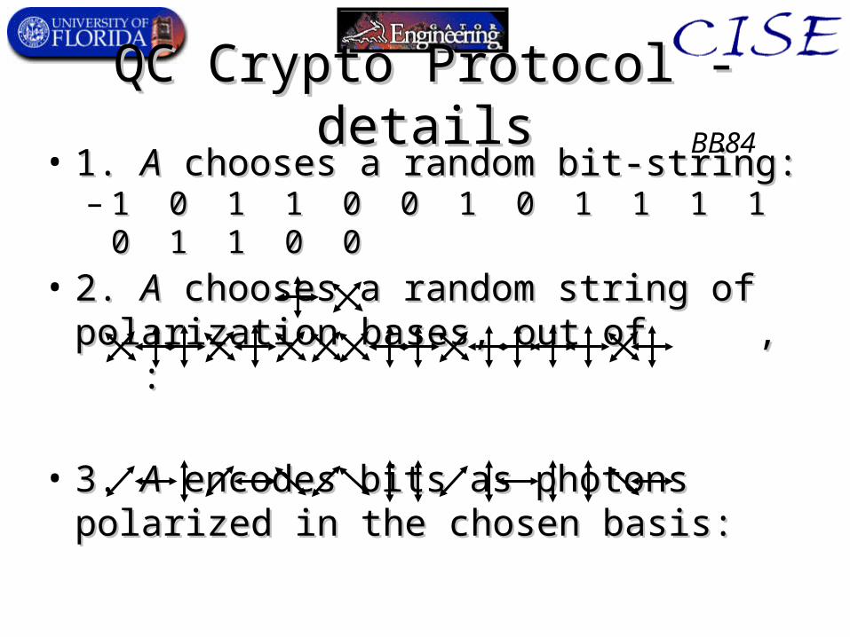
QC Crypto Protocol - detailsQC Crypto Protocol - details• 1. 1. AA chooses a random bit-string: chooses a random bit-string:
– 1 0 1 1 0 0 1 0 1 1 1 1 0 1 1 0 01 0 1 1 0 0 1 0 1 1 1 1 0 1 1 0 0
• 2. 2. AA chooses a random string of polarization chooses a random string of polarization bases, out of , : bases, out of , :
• 3. 3. AA encodes bits as photons polarized in the encodes bits as photons polarized in the chosen basis:chosen basis:
BB84
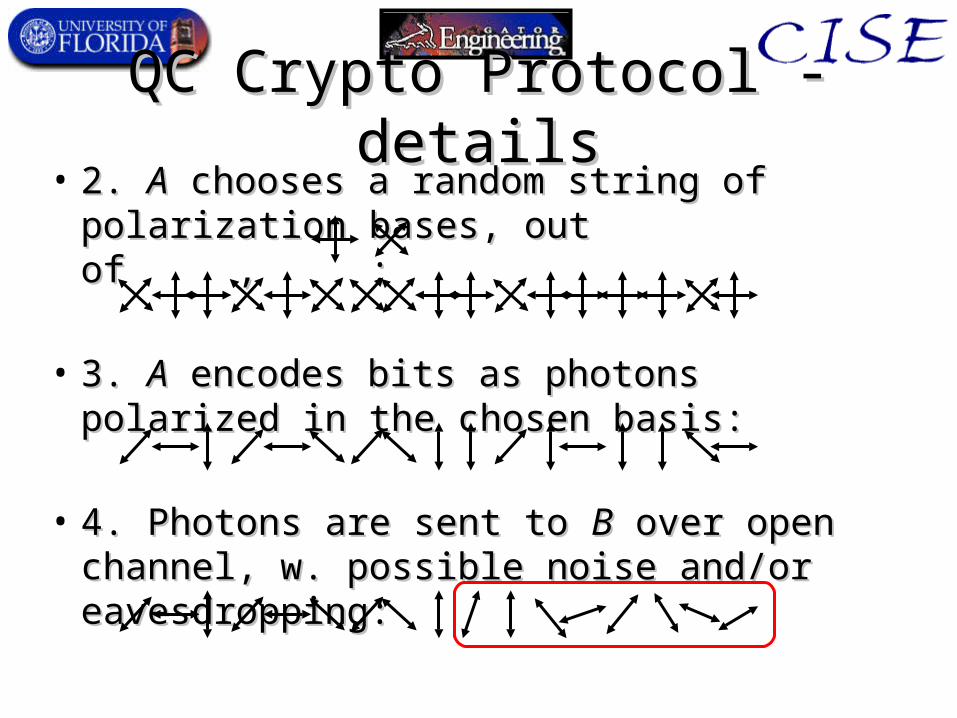
QC Crypto Protocol - detailsQC Crypto Protocol - details• 2. 2. AA chooses a random string of polarization chooses a random string of polarization
bases, out of , : bases, out of , :
• 3. 3. AA encodes bits as photons polarized in the encodes bits as photons polarized in the chosen basis:chosen basis:
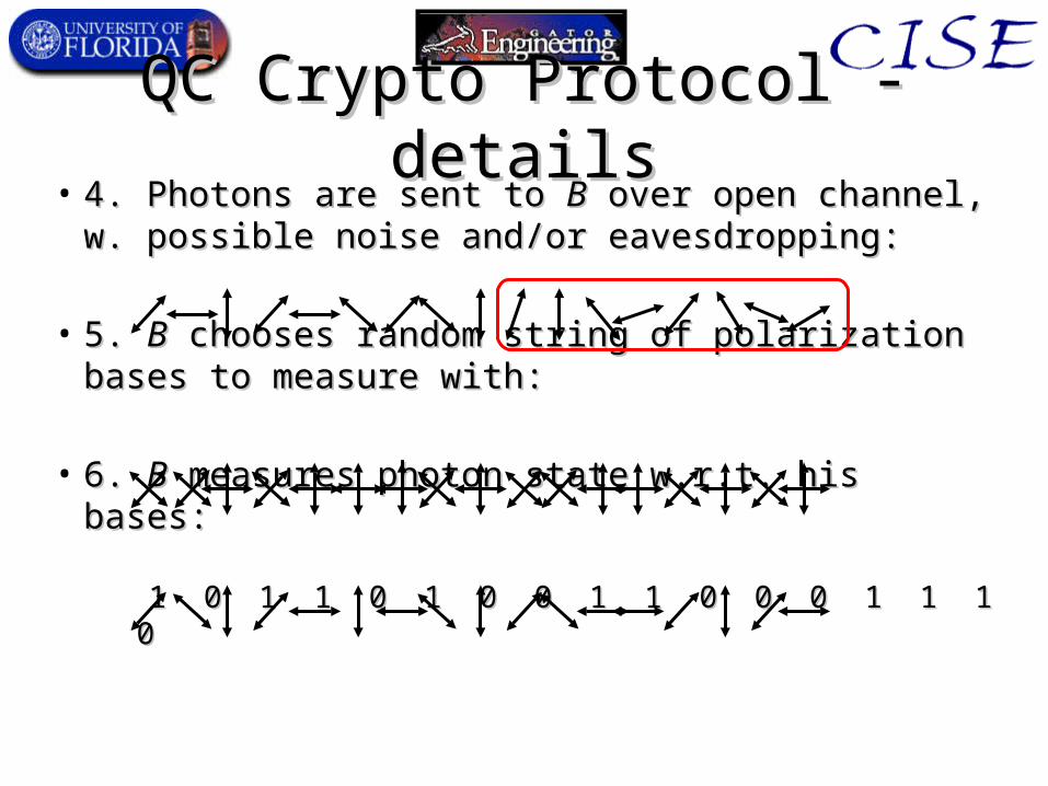
• 4. Photons are sent to 4. Photons are sent to BB over open channel, w. over open channel, w. possible noise and/or eavesdropping:possible noise and/or eavesdropping:
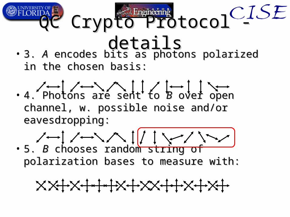
• 3. 3. AA encodes bits as photons polarized in the encodes bits as photons polarized in the chosen basis:chosen basis:
• 4. Photons are sent to 4. Photons are sent to BB over open channel, w. over open channel, w. possible noise and/or eavesdropping:possible noise and/or eavesdropping:
• 5. 5. BB chooses random string of polarization bases to chooses random string of polarization bases to measure with:measure with:
QC Crypto Protocol - detailsQC Crypto Protocol - details
• 4. Photons are sent to 4. Photons are sent to BB over open channel, w. over open channel, w. possible noise and/or eavesdropping:possible noise and/or eavesdropping:
• 5. 5. BB chooses random string of polarization chooses random string of polarization bases to measure with:bases to measure with:
• 6. 6. BB measures photon state w.r.t. his bases: measures photon state w.r.t. his bases:
1 0 1 1 0 1 0 0 1 1 0 0 0 1 1 1 01 0 1 1 0 1 0 0 1 1 0 0 0 1 1 1 0
QC Crypto Protocol - detailsQC Crypto Protocol - details
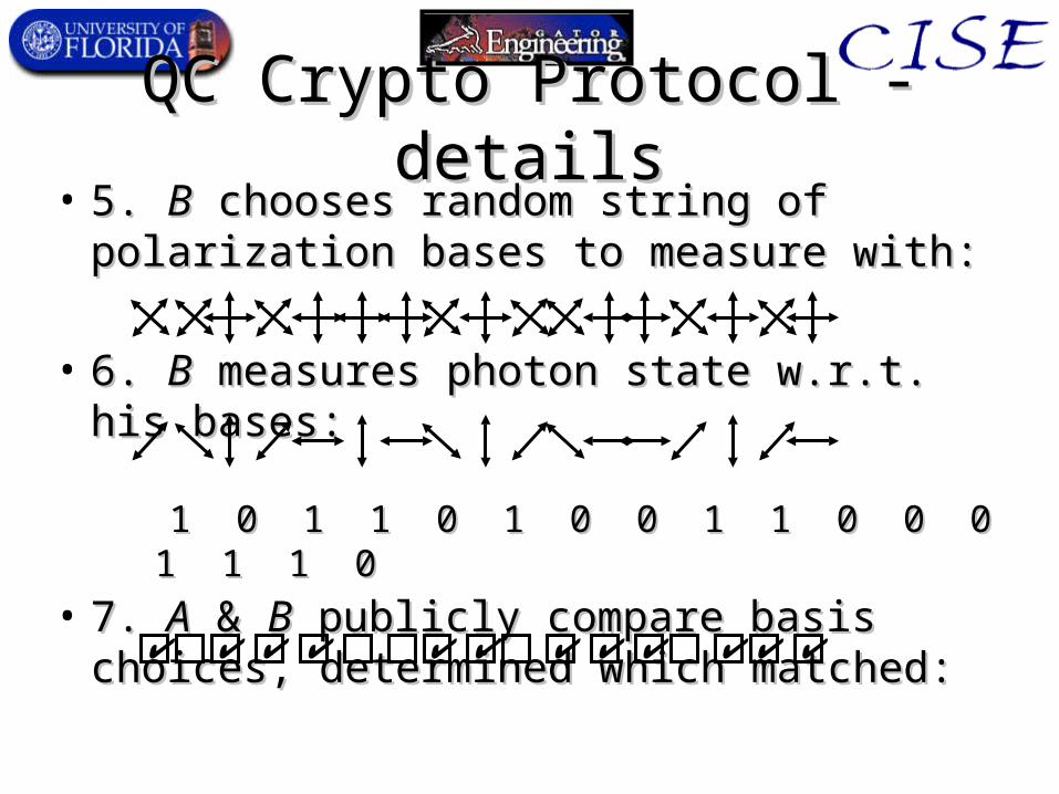
• 5. 5. BB chooses random string of polarization chooses random string of polarization bases to measure with:bases to measure with:
• 6. 6. BB measures photon state w.r.t. his bases: measures photon state w.r.t. his bases:
1 0 1 1 0 1 0 0 1 1 0 0 0 1 1 1 01 0 1 1 0 1 0 0 1 1 0 0 0 1 1 1 0
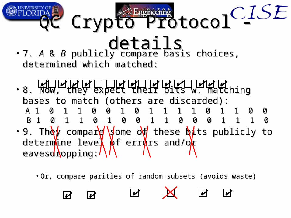
• 7. 7. AA & & BB publicly compare basis choices, publicly compare basis choices, determined which matched:determined which matched:
QC Crypto Protocol - detailsQC Crypto Protocol - details
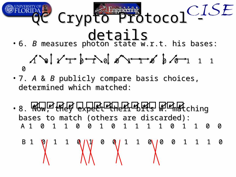
• 6. 6. BB measures photon state w.r.t. his bases: measures photon state w.r.t. his bases:
1 0 1 1 0 1 0 0 1 1 0 0 0 1 1 1 01 0 1 1 0 1 0 0 1 1 0 0 0 1 1 1 0
• 7. 7. AA & & BB publicly compare basis choices, publicly compare basis choices, determined which matched:determined which matched:
• 8. Now, they expect their bits w. matching bases 8. Now, they expect their bits w. matching bases to match (others are discarded):to match (others are discarded):A 1 0 1 1 0 0 1 0 1 1 1 1 0 1 1 0 0 A 1 0 1 1 0 0 1 0 1 1 1 1 0 1 1 0 0 B 1 0 1 1 0 1 0 0 1 1 0 0 0 1 1 1 0B 1 0 1 1 0 1 0 0 1 1 0 0 0 1 1 1 0
QC Crypto Protocol - detailsQC Crypto Protocol - details
• 7. 7. AA & & BB publicly compare basis choices, determined publicly compare basis choices, determined which matched:which matched:
• 8. Now, they expect their bits w. matching bases to 8. Now, they expect their bits w. matching bases to match (others are discarded):match (others are discarded):A 1 0 1 1 0 0 1 0 1 1 1 1 0 1 1 0 0 A 1 0 1 1 0 0 1 0 1 1 1 1 0 1 1 0 0 B 1 0 1 1 0 1 0 0 1 1 0 0 0 1 1 1 0B 1 0 1 1 0 1 0 0 1 1 0 0 0 1 1 1 0
• 9. They compare some of these bits publicly to 9. They compare some of these bits publicly to determine level of errors and/or eavesdropping:determine level of errors and/or eavesdropping:
• Or, compare parities of random subsets (avoids waste)Or, compare parities of random subsets (avoids waste)
QC Crypto Protocol - detailsQC Crypto Protocol - details
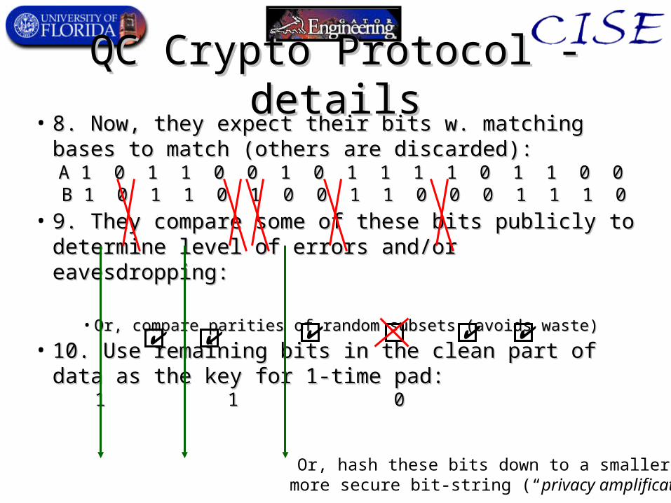
• 8. Now, they expect their bits w. matching bases to 8. Now, they expect their bits w. matching bases to match (others are discarded):match (others are discarded):A 1 0 1 1 0 0 1 0 1 1 1 1 0 1 1 0 0 A 1 0 1 1 0 0 1 0 1 1 1 1 0 1 1 0 0 B 1 0 1 1 0 1 0 0 1 1 0 0 0 1 1 1 0B 1 0 1 1 0 1 0 0 1 1 0 0 0 1 1 1 0
• 9. They compare some of these bits publicly to 9. They compare some of these bits publicly to determine level of errors and/or eavesdropping:determine level of errors and/or eavesdropping:
• Or, compare parities of random subsets (avoids waste)Or, compare parities of random subsets (avoids waste)
• 10. Use remaining bits in the clean part of data as the 10. Use remaining bits in the clean part of data as the key for 1-time pad:key for 1-time pad: 1 1 01 1 0
QC Crypto Protocol - detailsQC Crypto Protocol - details
Or, hash these bits down to a smaller butmore secure bit-string (“privacy amplification”)
Quantum Crypto ScalabilityQuantum Crypto Scalability• Optic fiber lengths Optic fiber lengths ~60-100 km not feasible due to ~60-100 km not feasible due to
attenuation.attenuation.• Free-space (air/vacuum) transmission being Free-space (air/vacuum) transmission being
explored.explored.– Useful in networks of orbiting satellites?Useful in networks of orbiting satellites?
• Given quantum computers, can build Given quantum computers, can build quantum quantum repeatersrepeaters that apply quantum error correction to that apply quantum error correction to clean up noisy signals?clean up noisy signals?– Can then maintain secure quantum cryptography Can then maintain secure quantum cryptography
throughout large networks (quantum internet?)throughout large networks (quantum internet?)– Research topic currently under investigation...Research topic currently under investigation...
Physical Implementations of Physical Implementations of Quantum ComputingQuantum Computing
Implementation RequirementsImplementation Requirements• 1. Scalable physical system w. well-characterized 1. Scalable physical system w. well-characterized
qubits.qubits.– Internal/external coupling parameters accurately known.Internal/external coupling parameters accurately known.
• 2. Initializability to a standardized state.2. Initializability to a standardized state.– Necessary for error correction.Necessary for error correction.– Speed of cooling/measurement is important.Speed of cooling/measurement is important.
• 3. Decoherence time >> gate operation time3. Decoherence time >> gate operation time– >10>1044-10-1055x for robust, fault-tolerant operationx for robust, fault-tolerant operation– Only Only computationalcomputational degrees of freedom need long degrees of freedom need long
decoherence times.decoherence times.
DiVincenzo ‘00
Implementation Reqs., Implementation Reqs., cont.cont.• 4. A Universal set of quantum gate operations4. A Universal set of quantum gate operations
– Controllable interactions generating desired Controllable interactions generating desired UUs.s.– 1- and 2-body interactions suffice1- and 2-body interactions suffice– Parallel ops are necessary for fault-tolerance.Parallel ops are necessary for fault-tolerance.
• 5. Bit-specific, amplifiable measurements5. Bit-specific, amplifiable measurements– High High quantum efficiencyquantum efficiency, or else redundancy., or else redundancy.– Shouldn’t disturb the rest of the computer.Shouldn’t disturb the rest of the computer.
Also for quantum crypto, comm., & distributed Also for quantum crypto, comm., & distributed computing:computing:
• 6. Faithful transmission of “flying qubits.”6. Faithful transmission of “flying qubits.”• 7. Interconversion btw. stationary & flying.7. Interconversion btw. stationary & flying.