Quantum Dynamics of a Kicked Harmonic

Oscillator

Quantum Dynamics of a Kicked Harmonic

OscillatorLaura Ingalls HuntleyProf. Calvin Stubbins

Franklin & Marshall CollegeDepartment of Physics & Astronomy

12 May 2006

Laura Ingalls HuntleyProf. Calvin Stubbins

Franklin & Marshall CollegeDepartment of Physics & Astronomy

12 May 2006

Presentation OutlinePresentation Outline

• Introduction to Coherent States• The Model and Solving the Schrödinger

Equation– The Probability Distribution and Coherent States– The Average Energy

• The General Potential– The Heisenberg Picture Method– The Infinite Series Method

• The Delta-Kicked Harmonic Oscillator– The Heisenberg Picture Method– The Infinite Series Method

• Conclusion

• Introduction to Coherent States• The Model and Solving the Schrödinger

Equation– The Probability Distribution and Coherent States– The Average Energy

• The General Potential– The Heisenberg Picture Method– The Infinite Series Method

• The Delta-Kicked Harmonic Oscillator– The Heisenberg Picture Method– The Infinite Series Method

• Conclusion

Introduction to Coherent StatesIntroduction to Coherent States

• Discovered in 1926 by Erwin Schrödinger as part of his description of wave mechanics.

• Schrödinger described non-stationary states of the quantum harmonic oscillator that preserve the shape of the wave packet and have classical motion.

• Coherent states have applications in atomic interactions, optics, Bose-Einstein condensation, laser-trapping of ions, and quantum electrodynamics.

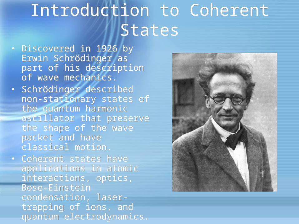
• Discovered in 1926 by Erwin Schrödinger as part of his description of wave mechanics.

• Schrödinger described non-stationary states of the quantum harmonic oscillator that preserve the shape of the wave packet and have classical motion.

• Coherent states have applications in atomic interactions, optics, Bose-Einstein condensation, laser-trapping of ions, and quantum electrodynamics.

Minimum-Uncertainty Coherent States

Minimum-Uncertainty Coherent States

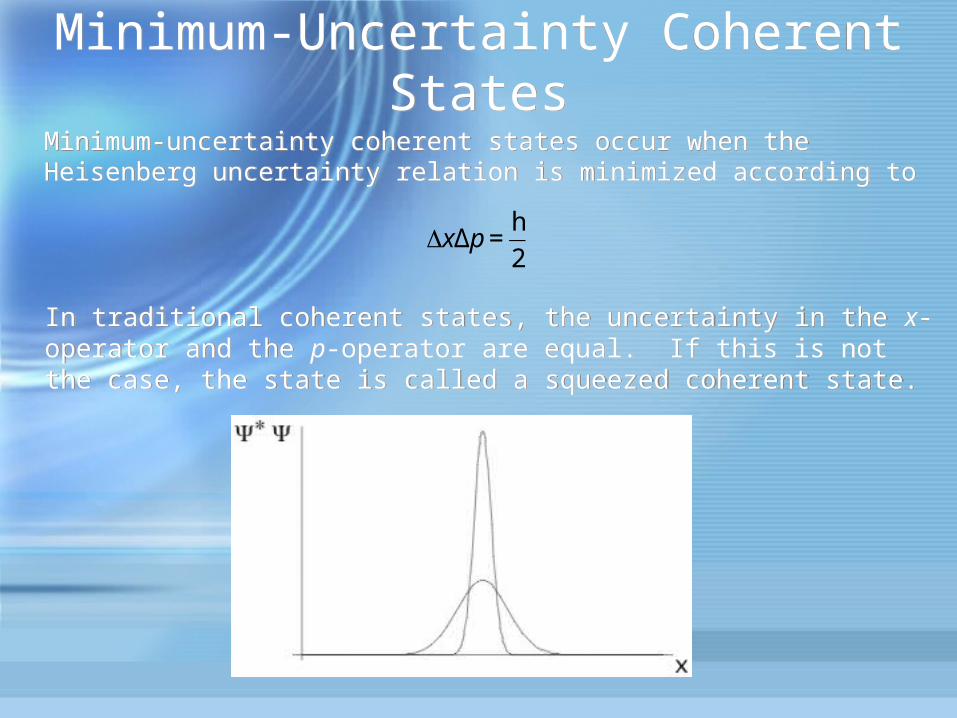
Minimum-uncertainty coherent states occur when the Heisenberg uncertainty relation is minimized according to Minimum-uncertainty coherent states occur when the Heisenberg uncertainty relation is minimized according to

€

ΔxΔp =h

2.

In traditional coherent states, the uncertainty in the x-operator and the p-operator are equal. If this is not the case, the state is called a squeezed coherent state.

In traditional coherent states, the uncertainty in the x-operator and the p-operator are equal. If this is not the case, the state is called a squeezed coherent state.

Displacement-Operator Coherent StatesDisplacement-Operator Coherent States

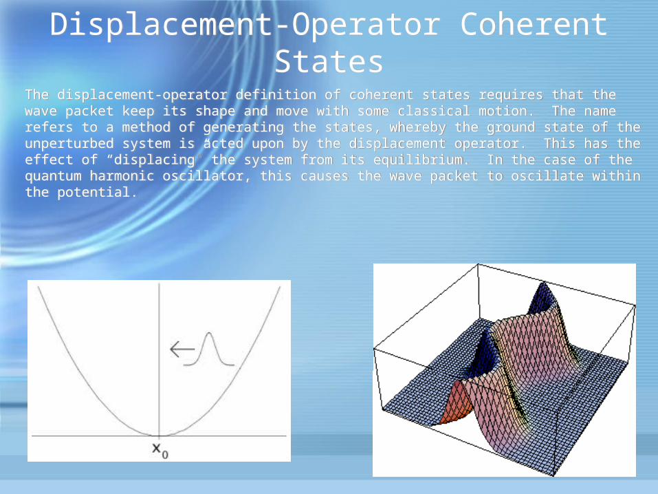
The displacement-operator definition of coherent states requires that the wave packet keep its shape and move with some classical motion. The name refers to a method of generating the states, whereby the ground state of the unperturbed system is acted upon by the displacement operator. This has the effect of “displacing” the system from its equilibrium. In the case of the quantum harmonic oscillator, this causes the wave packet to oscillate within the potential.

The displacement-operator definition of coherent states requires that the wave packet keep its shape and move with some classical motion. The name refers to a method of generating the states, whereby the ground state of the unperturbed system is acted upon by the displacement operator. This has the effect of “displacing” the system from its equilibrium. In the case of the quantum harmonic oscillator, this causes the wave packet to oscillate within the potential.

Annihilation-Operator Coherent StatesAnnihilation-Operator Coherent States

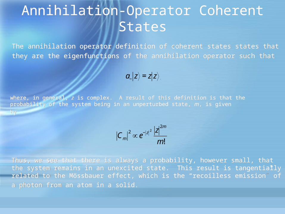
The annihilation operator definition of coherent states states that they are the eigenfunctions of the annihilation operator such that

The annihilation operator definition of coherent states states that they are the eigenfunctions of the annihilation operator such that

€

a− z = z z ,

where, in general, z is complex. A result of this definition is that the probability of the system being in an unperturbed state, m, is givenby

where, in general, z is complex. A result of this definition is that the probability of the system being in an unperturbed state, m, is givenby

€

Cm

2∝ e− z

2 z2m

m!.

Thus, we see that there is always a probability, however small, that the system remains in an unexcited state. This result is tangentially related to the Mössbauer effect, which is the “recoilless emission” of

a photon from an atom in a solid.

Thus, we see that there is always a probability, however small, that the system remains in an unexcited state. This result is tangentially related to the Mössbauer effect, which is the “recoilless emission” of

a photon from an atom in a solid.

The ModelThe Model

€

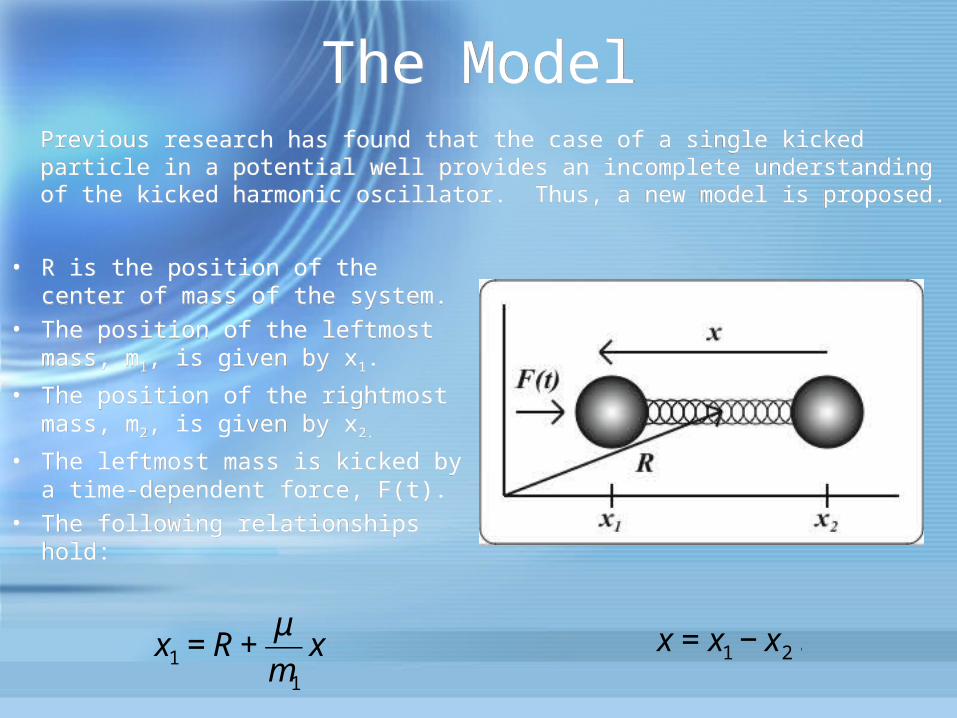
x1 = R +μ

m1

x

€

x = x1 − x2.

• R is the position of the center of mass of the system.

• The position of the leftmost mass, m1, is given by x1.

• The position of the rightmost mass, m2, is given by x2.

• The leftmost mass is kicked by a time-dependent force, F(t).

• The following relationships hold:

• R is the position of the center of mass of the system.

• The position of the leftmost mass, m1, is given by x1.

• The position of the rightmost mass, m2, is given by x2.

• The leftmost mass is kicked by a time-dependent force, F(t).

• The following relationships hold:

Previous research has found that the case of a single kicked particle in a potential well provides an incomplete understanding of the kicked harmonic oscillator. Thus, a new model is proposed.

Previous research has found that the case of a single kicked particle in a potential well provides an incomplete understanding of the kicked harmonic oscillator. Thus, a new model is proposed.

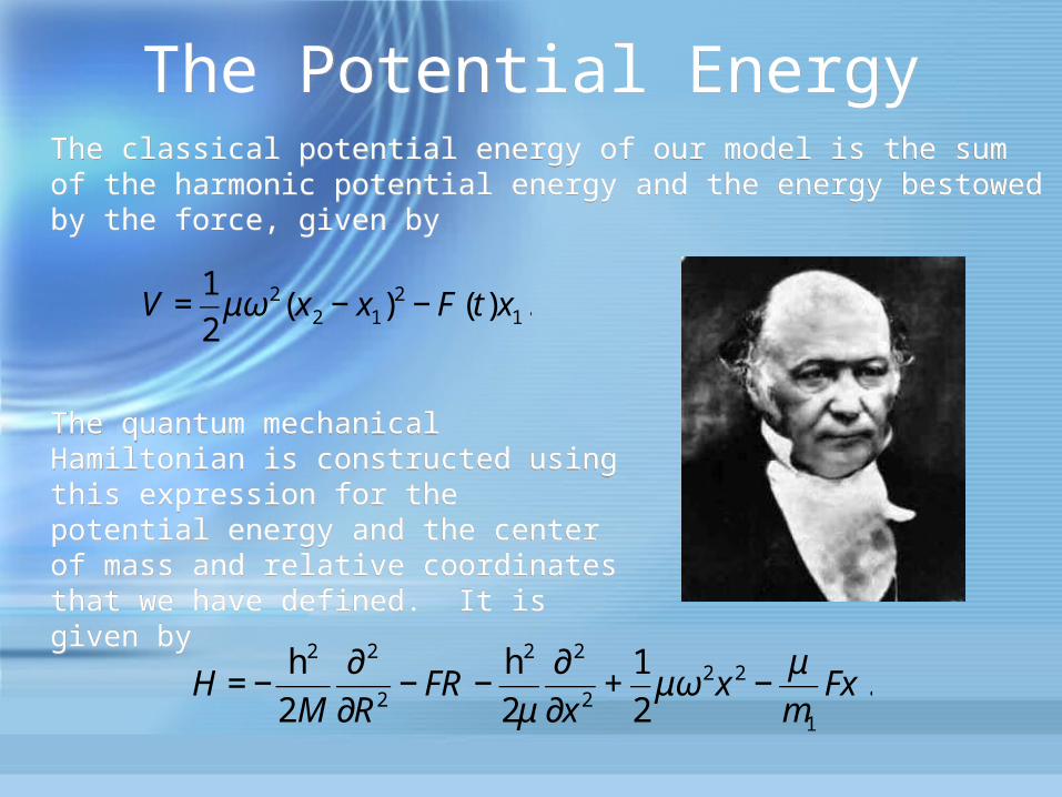
The Potential EnergyThe Potential EnergyThe classical potential energy of our model is the sum of the harmonic potential energy and the energy bestowed by the force, given by

The classical potential energy of our model is the sum of the harmonic potential energy and the energy bestowed by the force, given by

€

V =1

2μω2(x2 − x1)

2 − F(t)x1.

The quantum mechanical Hamiltonian is constructed using this expression for the potential energy and the center of mass and relative coordinates that we have defined. It is given by

The quantum mechanical Hamiltonian is constructed using this expression for the potential energy and the center of mass and relative coordinates that we have defined. It is given by

€

H = −h2

2M

∂ 2

∂R2− FR −

h2

2μ

∂ 2

∂x 2+

1

2μω2x 2 −

μ

m1

Fx.

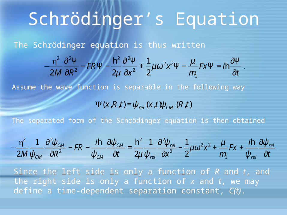
Schrödinger’s EquationSchrödinger’s EquationThe Schrödinger equation is thus writtenThe Schrödinger equation is thus written

€

−h2

2M

∂ 2Ψ

∂R2− FRΨ −

h2

2μ

∂ 2Ψ

∂x 2+

1

2μω2x 2Ψ −

μ

m1

FxΨ = ih∂Ψ

∂t.

€

Ψ(x,R, t) =ψ rel (x, t)ψCM (R, t).

€

−h2

2M

1

ψCM

∂ 2ψCM

∂R2− FR −

ih

ψCM

∂ψCM

∂t=

h2

2μ

1

ψ rel

∂ 2ψ rel

∂x 2−

1

2μω2x 2 +

μ

m1

Fx +ih

ψ rel

∂ψ rel

∂t.

Assume the wave function is separable in the following wayAssume the wave function is separable in the following way

The separated form of the Schrödinger equation is then obtainedThe separated form of the Schrödinger equation is then obtained

Since the left side is only a function of R and t, and the right side is only a function of x and t, we may define a time-dependent separation constant, C(t).

Since the left side is only a function of R and t, and the right side is only a function of x and t, we may define a time-dependent separation constant, C(t).

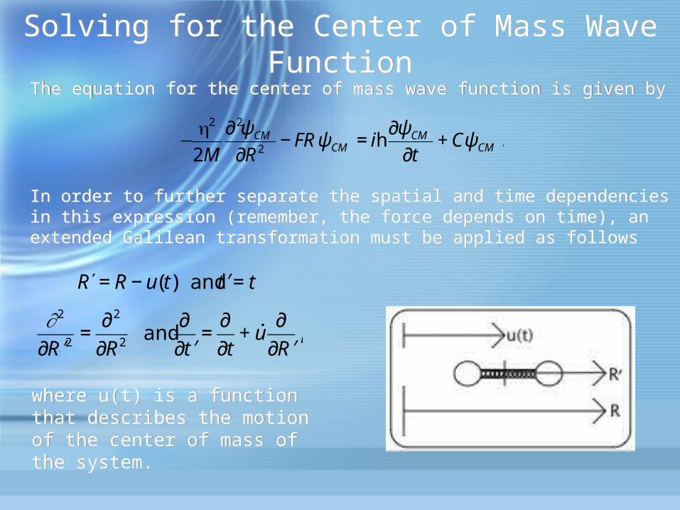
In order to further separate the spatial and time dependencies in this expression (remember, the force depends on time), an extended Galilean transformation must be applied as follows

In order to further separate the spatial and time dependencies in this expression (remember, the force depends on time), an extended Galilean transformation must be applied as follows

€

′ R = R − u(t) and ′ t = t

€

∂2

∂ ′ R 2=

∂ 2

∂R2 and

∂

∂ ′ t =

∂

∂t+ ˙ u

∂

∂ ′ R ,

The equation for the center of mass wave function is given byThe equation for the center of mass wave function is given by

Solving for the Center of Mass Wave Function

Solving for the Center of Mass Wave Function

€

−h2

2M

∂ 2ψCM

∂R2− FRψCM = ih

∂ψCM

∂t+ CψCM .

where u(t) is a function that describes the motion of the center of mass of the system.

where u(t) is a function that describes the motion of the center of mass of the system.

€

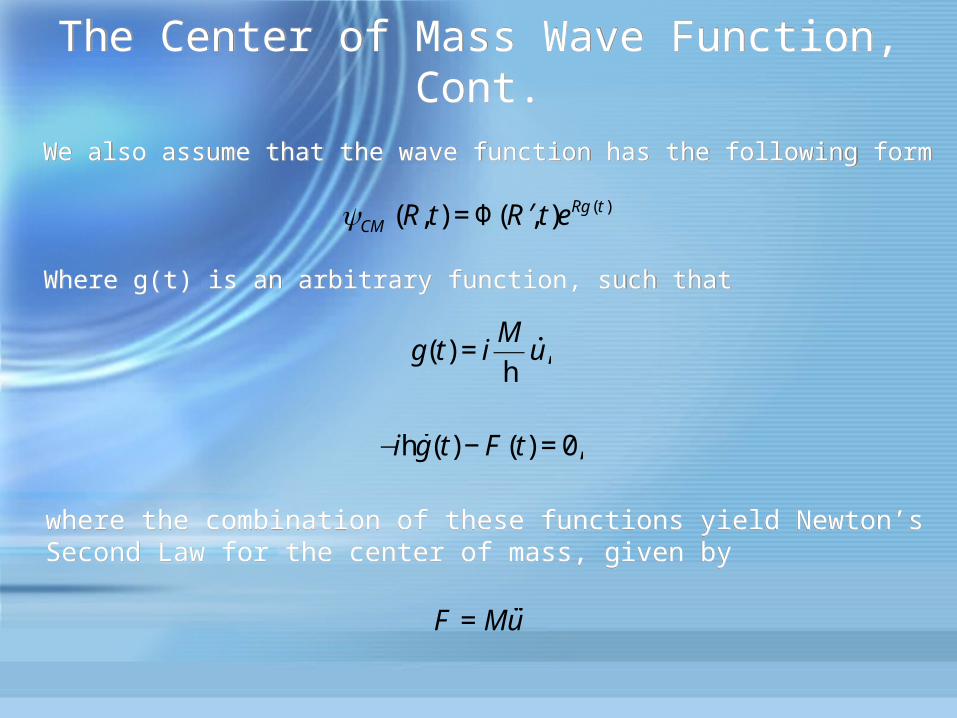
F = M˙ ̇ u .

€

ψCM (R, t) = Φ( ′ R , t)eRg(t ).

€

g(t) = iM

h˙ u ,

We also assume that the wave function has the following formWe also assume that the wave function has the following form

Where g(t) is an arbitrary function, such that Where g(t) is an arbitrary function, such that

€

−ih˙ g (t) − F(t) = 0,

where the combination of these functions yield Newton’s Second Law for the center of mass, given by where the combination of these functions yield Newton’s Second Law for the center of mass, given by

The Center of Mass Wave Function, Cont.The Center of Mass Wave Function, Cont.

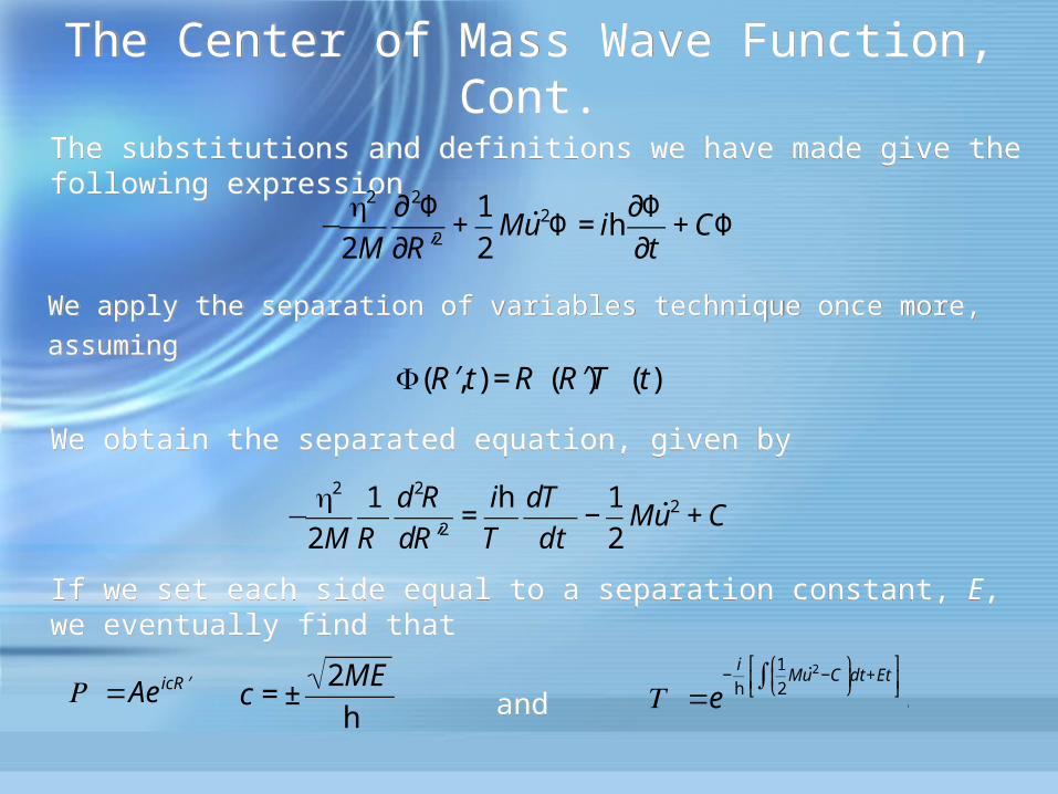
The substitutions and definitions we have made give the following expressionThe substitutions and definitions we have made give the following expression

The Center of Mass Wave Function, Cont.The Center of Mass Wave Function, Cont.

€

−h2

2M

∂ 2Φ

∂ ′ R 2+

1

2M ˙ u 2Φ = ih

∂Φ

∂t+ CΦ.

€

Φ( ′ R , t) = R ( ′ R )T (t).

€

c = ±2ME

h

€

−h2

2M

1

R

d2R

d ′ R 2=

ih

T

dT

dt−

1

2M ˙ u 2 + C.

€

R =Ae ic ′ R

We apply the separation of variables technique once more, assuming

We apply the separation of variables technique once more, assuming

We obtain the separated equation, given byWe obtain the separated equation, given by

If we set each side equal to a separation constant, E, we eventually find thatIf we set each side equal to a separation constant, E, we eventually find that

andand

€

T =e−

i

h

1

2M ˙ u 2 −C

⎛

⎝ ⎜

⎞

⎠ ⎟∫ dt +Et

⎡

⎣ ⎢

⎤

⎦ ⎥.

The Center of Mass Wave Function, Cont.The Center of Mass Wave Function, Cont.

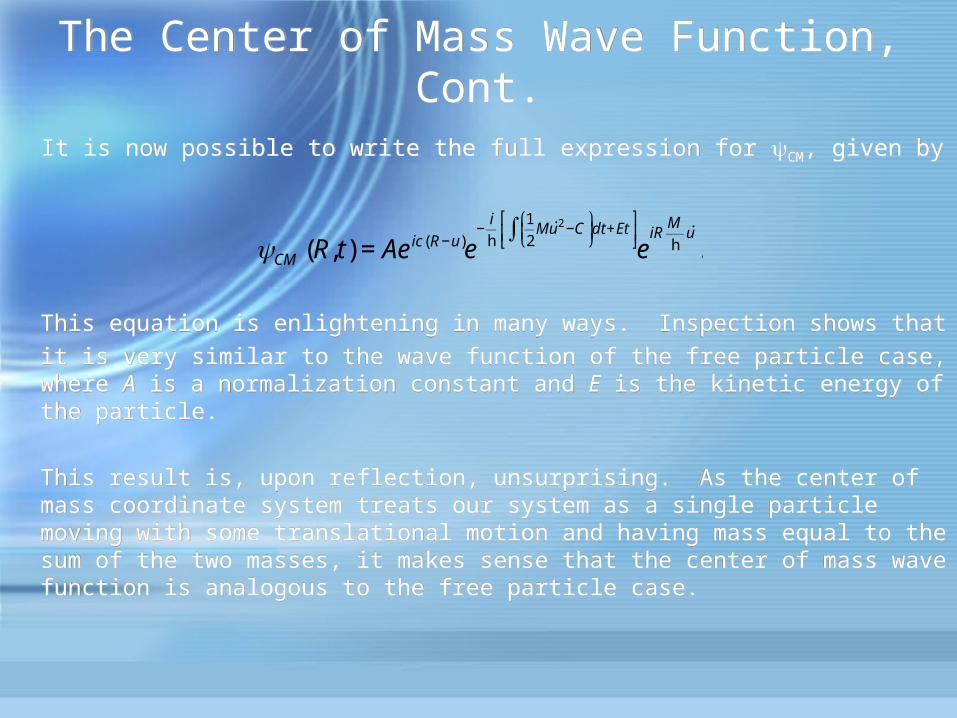
It is now possible to write the full expression for ψCM, given by It is now possible to write the full expression for ψCM, given by

€

ψCM (R, t) = Ae ic(R−u)e−

i

h

1

2M ˙ u 2 −C

⎛

⎝ ⎜

⎞

⎠ ⎟∫ dt +Et

⎡

⎣ ⎢

⎤

⎦ ⎥e

iRM

h˙ u .

This equation is enlightening in many ways. Inspection shows that it is very similar to the wave function of the free particle case, where A is a normalization constant and E is the kinetic energy of the particle.

This result is, upon reflection, unsurprising. As the center of mass coordinate system treats our system as a single particle moving with some translational motion and having mass equal to the sum of the two masses, it makes sense that the center of mass wave function is analogous to the free particle case.

This equation is enlightening in many ways. Inspection shows that it is very similar to the wave function of the free particle case, where A is a normalization constant and E is the kinetic energy of the particle.

This result is, upon reflection, unsurprising. As the center of mass coordinate system treats our system as a single particle moving with some translational motion and having mass equal to the sum of the two masses, it makes sense that the center of mass wave function is analogous to the free particle case.

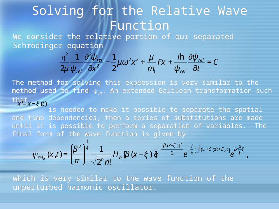
Solving for the Relative Wave FunctionSolving for the Relative Wave FunctionWe consider the relative portion of our separated Schrödinger equationWe consider the relative portion of our separated Schrödinger equation

€

h2

2μ

1

ψ rel

∂ 2ψ rel

∂x 2−

1

2μω2x 2 +

μ

m1

Fx +ih

ψ rel

∂ψ rel

∂t= C.

The method for solving this expression is very similar to the method used to find ψCM. An extended Galilean transformation such that

is needed to make it possible to separate the spatial and time dependencies, then a series of substitutions are made until it is possible to perform a separation of variables. The final form of the wave function is given by

The method for solving this expression is very similar to the method used to find ψCM. An extended Galilean transformation such that

is needed to make it possible to separate the spatial and time dependencies, then a series of substitutions are made until it is possible to perform a separation of variables. The final form of the wave function is given by

€

ψreln(x, t) =

β 2

π

⎛

⎝ ⎜

⎞

⎠ ⎟

1

4 1

2n n!Hn[β (x −ξ )]e

−β x−ξ( )[ ]

2

2 e−

i

hL +C( )∫ dt +Ent[ ]

eix

μ

h˙ ξ ,

€

x'= x −ξ (t)

which is very similar to the wave function of the unperturbed harmonic oscillator. which is very similar to the wave function of the unperturbed harmonic oscillator.

The Complete Wave FunctionThe Complete Wave Function

€

Ψn (x,R, t) = Aβ 2

π

⎛

⎝ ⎜

⎞

⎠ ⎟

1

4 1

2n n!Hn[β (x −ξ )]e

−β x−ξ( )[ ]

2

2 eix

μ

h˙ ξ e

iRM

h˙ u e ic(R−u).e

−i

hLdt +

1

2M ˙ u 2∫ dt +(E +En )t

⎛

⎝ ⎜

⎞

⎠ ⎟.

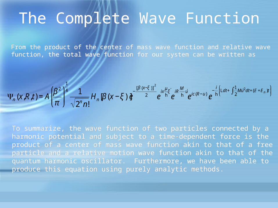
From the product of the center of mass wave function and relative wave function, the total wave function for our system can be written asFrom the product of the center of mass wave function and relative wave function, the total wave function for our system can be written as

To summarize, the wave function of two particles connected by a harmonic potential and subject to a time-dependent force is the product of a center of mass wave function akin to that of a free particle and a relative motion wave function akin to that of the quantum harmonic oscillator. Furthermore, we have been able to produce this equation using purely analytic methods.

To summarize, the wave function of two particles connected by a harmonic potential and subject to a time-dependent force is the product of a center of mass wave function akin to that of a free particle and a relative motion wave function akin to that of the quantum harmonic oscillator. Furthermore, we have been able to produce this equation using purely analytic methods.

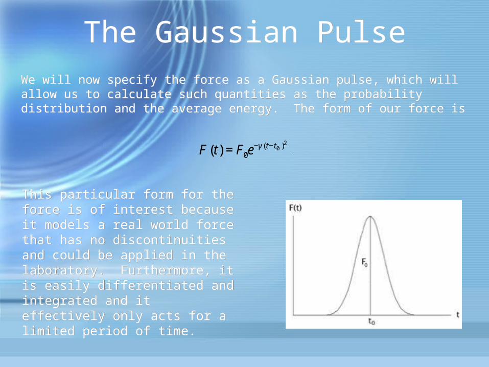
The Gaussian PulseThe Gaussian PulseWe will now specify the force as a Gaussian pulse, which will allow us to calculate such quantities as the probability distribution and the average energy. The form of our force is

We will now specify the force as a Gaussian pulse, which will allow us to calculate such quantities as the probability distribution and the average energy. The form of our force is

€

F(t) = F0e−γ ( t−t0 )2

.

This particular form for the force is of interest because it models a real world force that has no discontinuities and could be applied in the laboratory. Furthermore, it is easily differentiated and integrated and it effectively only acts for a limited period of time.

This particular form for the force is of interest because it models a real world force that has no discontinuities and could be applied in the laboratory. Furthermore, it is easily differentiated and integrated and it effectively only acts for a limited period of time.

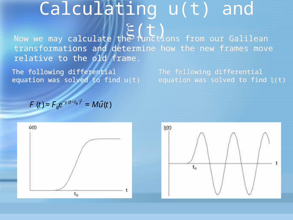
Calculating u(t) and (t)Calculating u(t) and (t)Now we may calculate the functions from our Galilean transformations and determine how the new frames move relative to the old frame.

Now we may calculate the functions from our Galilean transformations and determine how the new frames move relative to the old frame.

The following differential equation was solved to find u(t)The following differential equation was solved to find u(t)

The following differential equation was solved to find (t)The following differential equation was solved to find (t)

€

F(t) = F0e−γ ( t−t0 )2

= M˙ ̇ u (t).

€

μm1

F(t) = F0e−γ ( t−t0 )2

= μ ˙ ̇ ξ (t) + μω2ξ (t).

The Probability DistributionThe Probability Distribution

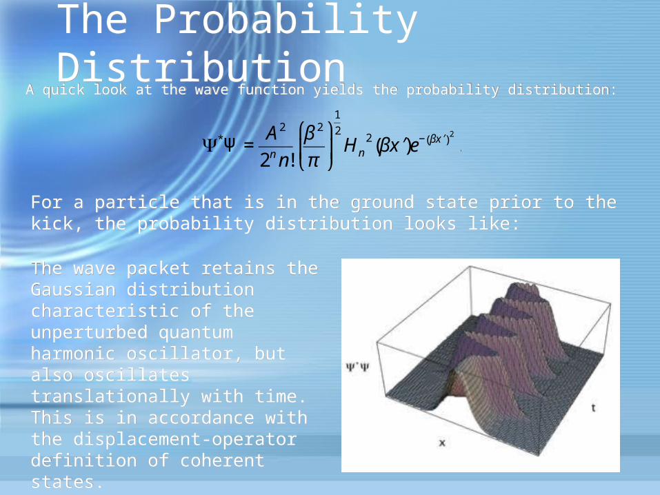
A quick look at the wave function yields the probability distribution:A quick look at the wave function yields the probability distribution:

€

Ψ*Ψ =A2

2n n!

β 2

π

⎛

⎝ ⎜

⎞

⎠ ⎟

1

2

Hn2(β ′ x )e− β ′ x ( )

2

.

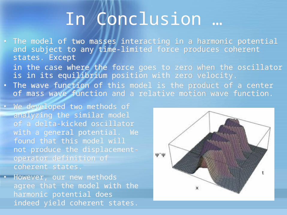
For a particle that is in the ground state prior to the kick, the probability distribution looks like:For a particle that is in the ground state prior to the kick, the probability distribution looks like:

The wave packet retains the Gaussian distribution characteristic of the unperturbed quantum harmonic oscillator, but also oscillates translationally with time. This is in accordance with the displacement-operator definition of coherent states.

The wave packet retains the Gaussian distribution characteristic of the unperturbed quantum harmonic oscillator, but also oscillates translationally with time. This is in accordance with the displacement-operator definition of coherent states.

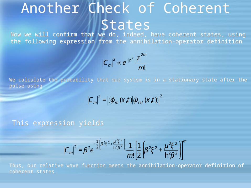
Another Check of Coherent StatesAnother Check of Coherent StatesNow we will confirm that we do, indeed, have coherent states, using the following expression from the annihilation-operator definitionNow we will confirm that we do, indeed, have coherent states, using the following expression from the annihilation-operator definition

€

Cm

2∝ e− z

2 z2m

m!.

€

Cm

2= β 2e

−1

2β 2ξ 2 +

μ 2ξ 2

h 2β 2

⎛

⎝ ⎜

⎞

⎠ ⎟ 1

m!

1

2β 2ξ 2 +

μ 2ξ 2

h2β 2

⎛

⎝ ⎜

⎞

⎠ ⎟

⎡

⎣ ⎢

⎤

⎦ ⎥

m

.

€

Cm

2= ϕ m (x, t) ψ rel (x, t)

2.

We calculate the probability that our system is in a stationary state after the pulse usingWe calculate the probability that our system is in a stationary state after the pulse using

This expression yieldsThis expression yields

Thus, our relative wave function meets the annihilation-operator definition of coherent states.Thus, our relative wave function meets the annihilation-operator definition of coherent states.

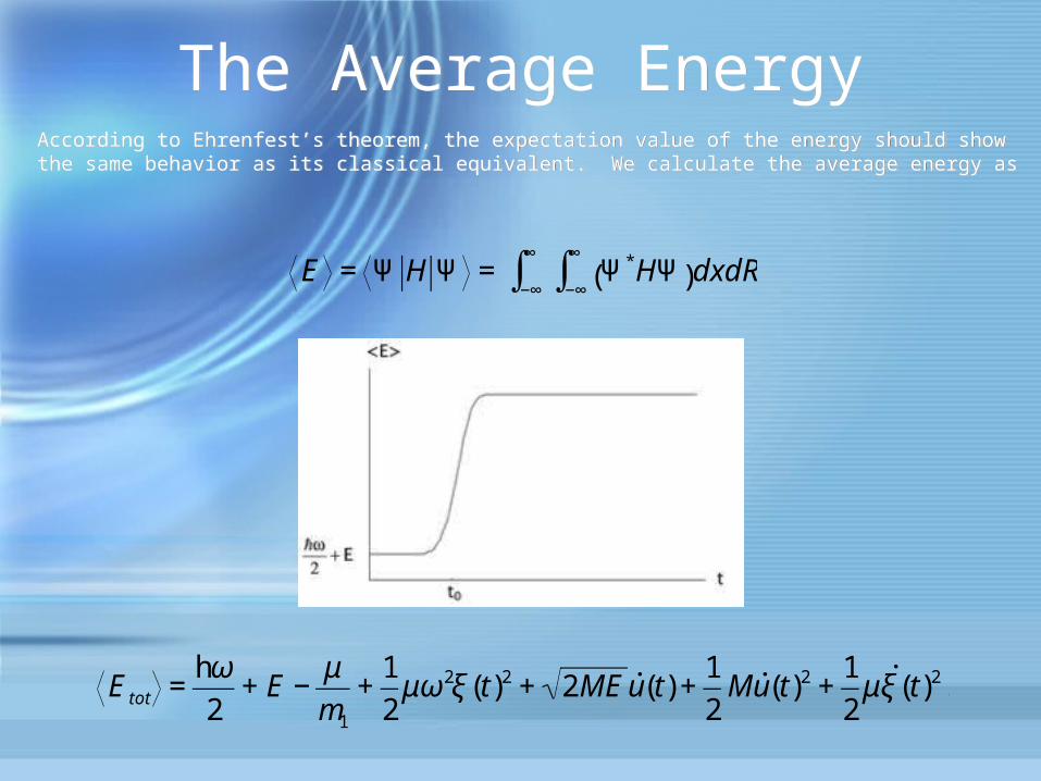
The Average EnergyThe Average EnergyAccording to Ehrenfest’s theorem, the expectation value of the energy should show the same behavior as its classical equivalent. We calculate the average energy asAccording to Ehrenfest’s theorem, the expectation value of the energy should show the same behavior as its classical equivalent. We calculate the average energy as

€

E = Ψ H Ψ = Ψ*HΨ( )dxdR−∞

∞

∫−∞

∞

∫

€

E tot =hω

2+ E −

μ

m1

+1

2μω2ξ (t)2 + 2ME ˙ u (t) +

1

2M ˙ u (t)2 +

1

2μ ˙ ξ (t)2 .

The General Potential and the Delta KickThe General Potential and the Delta Kick

We have shown that any time-limited force acting on our model produces coherent states. Now, we would like to generalize the potential in which our masses interact. In order to make our calculations more simple, we will assume a Dirac delta function form for the force, such that

Although this form is not exceedingly realistic, it allows us to expand our analysis of the system considerably. We will now develop two new methods for finding the resultant wave function of our two-particle model will a general potential and a delta-function force. The first step in developing these techniques is to return to the relative motion Schrödinger equation

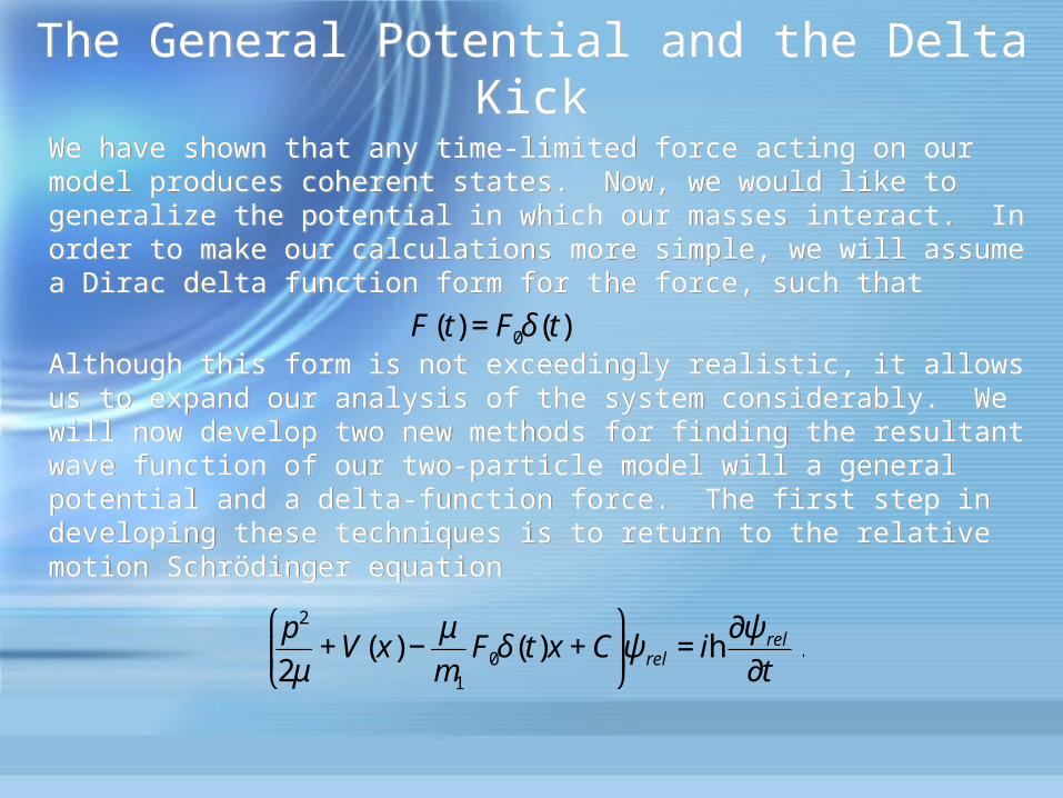
We have shown that any time-limited force acting on our model produces coherent states. Now, we would like to generalize the potential in which our masses interact. In order to make our calculations more simple, we will assume a Dirac delta function form for the force, such that

Although this form is not exceedingly realistic, it allows us to expand our analysis of the system considerably. We will now develop two new methods for finding the resultant wave function of our two-particle model will a general potential and a delta-function force. The first step in developing these techniques is to return to the relative motion Schrödinger equation

€

F(t) = F0δ(t).

€

p2

2μ+ V (x) −

μ

m1

F0δ(t)x + C ⎛

⎝ ⎜

⎞

⎠ ⎟ψ rel = ih

∂ψ rel

∂t.

The General Potential, cont.

The General Potential, cont.

€

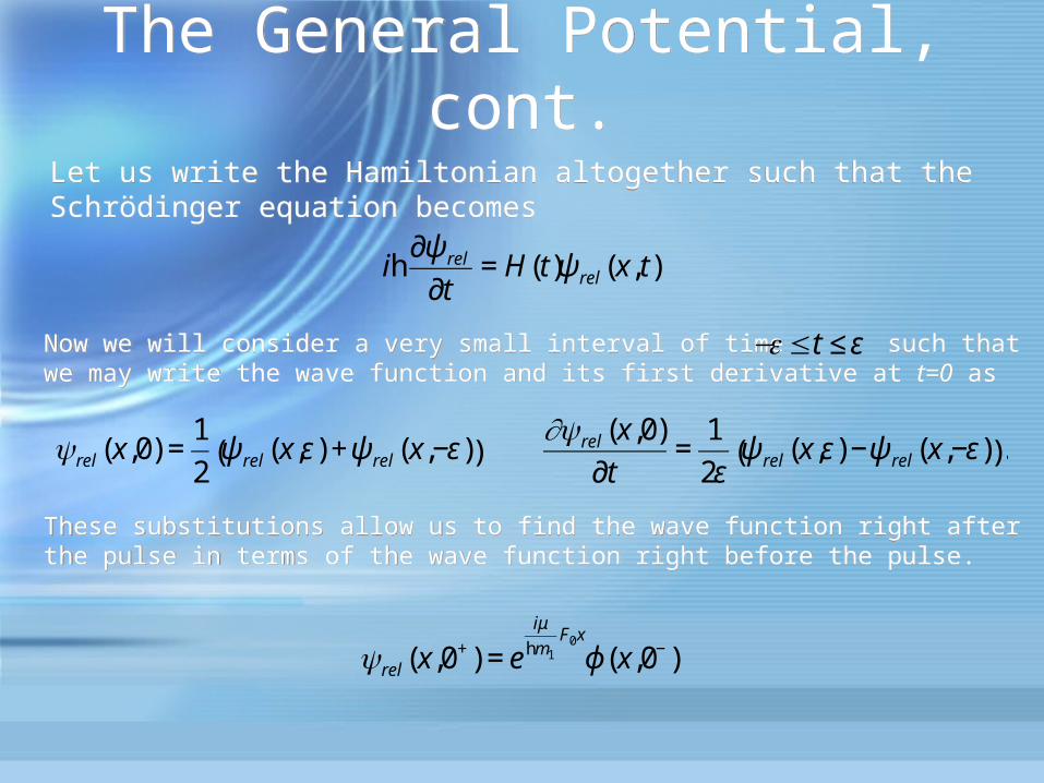
ih∂ψ rel

∂t= H(t)ψ rel (x, t).

Let us write the Hamiltonian altogether such that the Schrödinger equation becomesLet us write the Hamiltonian altogether such that the Schrödinger equation becomes

Now we will consider a very small interval of time such that we may write the wave function and its first derivative at t=0 asNow we will consider a very small interval of time such that we may write the wave function and its first derivative at t=0 as

€

−ε ≤t ≤ ε

€

ψrel (x,0) =1

2ψ rel (x,ε) +ψ rel (x,−ε)( )

€

∂ψrel (x,0)

∂t=

1

2εψ rel (x,ε) −ψ rel (x,−ε)( ).

These substitutions allow us to find the wave function right after the pulse in terms of the wave function right before the pulse.These substitutions allow us to find the wave function right after the pulse in terms of the wave function right before the pulse.

€

ψrel (x,0+) = eiμ

hm1

F0x

ϕ (x,0−).

The General Potential, cont.

The General Potential, cont.

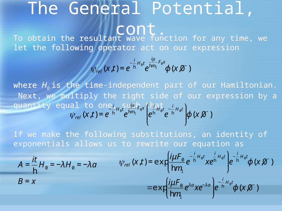
To obtain the resultant wave function for any time, we let the following operator act on our expressionTo obtain the resultant wave function for any time, we let the following operator act on our expression

where H0 is the time-independent part of our Hamiltonian. Next, we multiply the right side of our expression by a quantity equal to one, such that

where H0 is the time-independent part of our Hamiltonian. Next, we multiply the right side of our expression by a quantity equal to one, such that

If we make the following substitutions, an identity of exponentials allows us to rewrite our equation asIf we make the following substitutions, an identity of exponentials allows us to rewrite our equation as

€

ψrel (x, t) = e−

i

hH0t

eiμ

hm1

F0x

ϕ (x,0−),

€

ψrel (x, t) = e−

i

hH0t

eiμ

hm1

F0x

ei

hH0t

e−

i

hH0t ⎛

⎝ ⎜

⎞

⎠ ⎟ϕ (x,0−).

€

A =it

hH0 = −λH0 = −λa

B = x

€

ψrel (x, t) = expiμF0

hm1

e−

i

hH0t

xei

hH0t ⎛

⎝ ⎜

⎞

⎠ ⎟e

−i

hH0t

ϕ (x,0−)

€

=expiμF0

hm1

eλa xe−λa ⎛

⎝ ⎜

⎞

⎠ ⎟e

−i

hH0t

ϕ (x,0−).

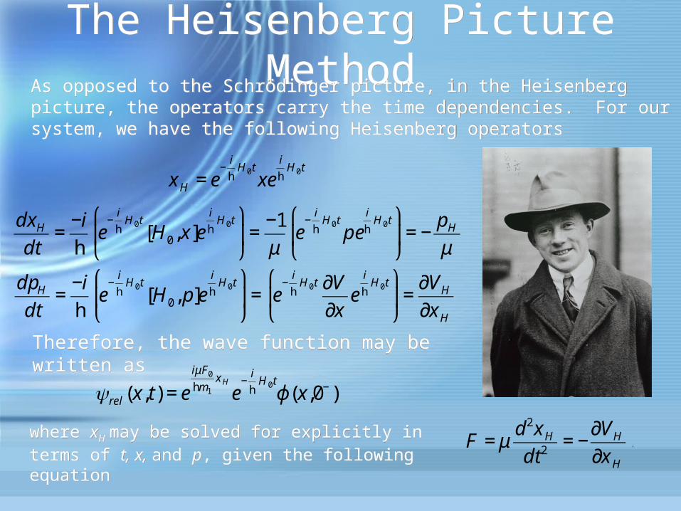
The Heisenberg Picture MethodThe Heisenberg Picture MethodAs opposed to the Schrödinger picture, in the Heisenberg picture, the operators carry the time dependencies. For our system, we have the following Heisenberg operators

As opposed to the Schrödinger picture, in the Heisenberg picture, the operators carry the time dependencies. For our system, we have the following Heisenberg operators

€

xH = e−

i

hH0t

xei

hH0t

€

dxH

dt=

−i

he

−i

hH0t

[H0,x]ei

hH0t ⎛

⎝ ⎜

⎞

⎠ ⎟=

−1

μe

−i

hH0t

pei

hH0t ⎛

⎝ ⎜

⎞

⎠ ⎟= −

pH

μ

€

dpH

dt=

−i

he

−i

hH0t

[H0, p]ei

hH0t ⎛

⎝ ⎜

⎞

⎠ ⎟= e

−i

hH0t ∂V

∂xe

i

hH0t ⎛

⎝ ⎜

⎞

⎠ ⎟=

∂VH

∂xH

.

Therefore, the wave function may be written asTherefore, the wave function may be written as

€

ψrel (x, t) = eiμF0

hm1

x H

e−

i

hH0t

ϕ (x,0−),

where xH may be solved for explicitly in terms of t, x, and p, given the following equationwhere xH may be solved for explicitly in terms of t, x, and p, given the following equation

€

F = μd2xH

dt 2= −

∂VH

∂xH

.

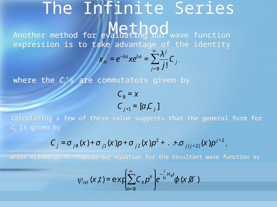
The Infinite Series MethodThe Infinite Series MethodAnother method for evaluating our wave function expression is to take advantage of the identity Another method for evaluating our wave function expression is to take advantage of the identity

€

xH = e−λa xeλa =λ j

j!C j

j= 0

∞

∑ ,

where the Cj’s are commutators given by where the Cj’s are commutators given by

Calculating a few of these value suggests that the general form for Cj is given by

Calculating a few of these value suggests that the general form for Cj is given by

€

C0 = x

C j +1 = [a,C j ].

€

C j = σ j 0(x) + σ j1(x)p + σ j 2(x) p2 + ...+ σ j( j +2)(x)p j +2,

which allows us to rewrite our equation for the resultant wave function aswhich allows us to rewrite our equation for the resultant wave function as

€

ψrel (x, t) = exp Ch ph

h= 0

∞

∑ ⎛

⎝ ⎜

⎞

⎠ ⎟e

−i

hH0t

ϕ (x,0−).

The Delta-Kicked Harmonic OscillatorThe Delta-Kicked Harmonic Oscillator

€

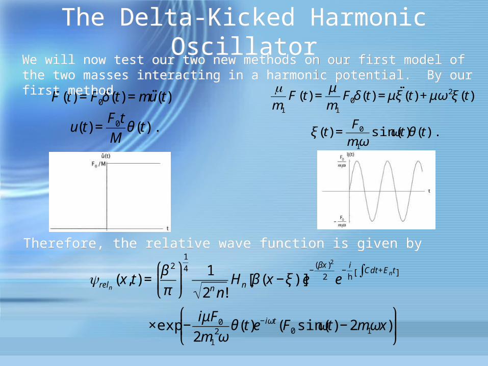
F(t) = F0δ(t) = m˙ ̇ u (t)

u(t) =F0t

Mθ(t).

€

μm1

F(t) =μ

m1

F0δ(t) = μ ˙ ̇ ξ (t) + μω2ξ (t)

ξ (t) =F0

m1ωsin(ωt)θ(t).

We will now test our two new methods on our first model of the two masses interacting in a harmonic potential. By our first methodWe will now test our two new methods on our first model of the two masses interacting in a harmonic potential. By our first method

Therefore, the relative wave function is given byTherefore, the relative wave function is given by

€

ψreln(x, t) =

β 2

π

⎛

⎝ ⎜

⎞

⎠ ⎟

1

4 1

2n n!Hn[β (x −ξ )]e

−(βx )2

2 e−

i

hC∫ dt +Ent[ ]

×exp −iμF0

2m12ω

θ(t)e−iωt (F0 sin(ωt) − 2m1ωx) ⎛

⎝ ⎜

⎞

⎠ ⎟.

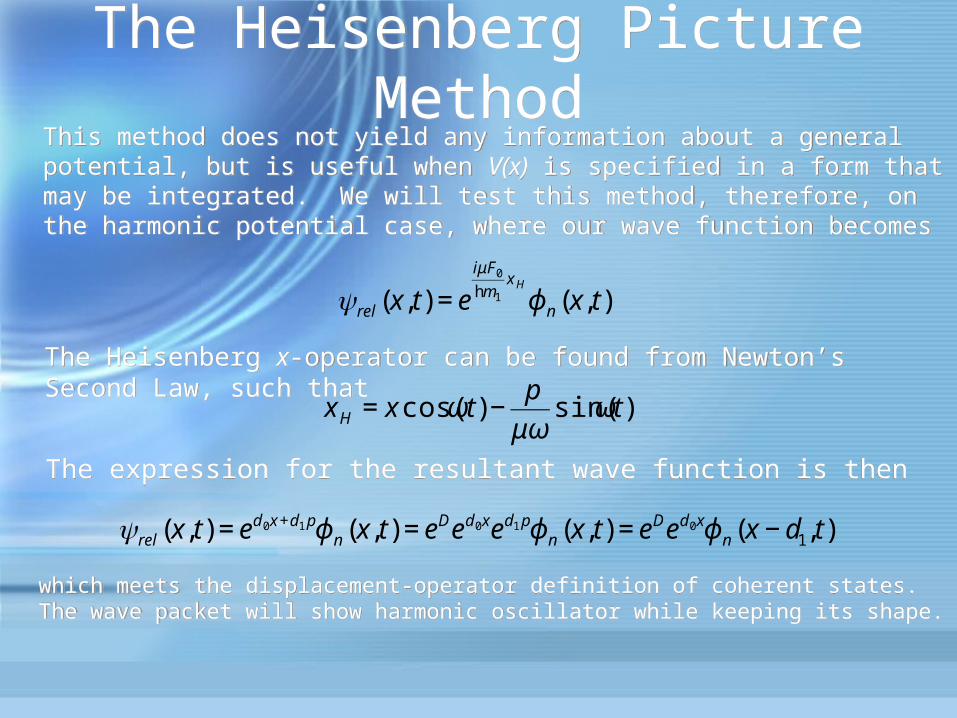
The Heisenberg Picture MethodThe Heisenberg Picture MethodThis method does not yield any information about a general potential, but is useful when V(x) is specified in a form that may be integrated. We will test this method, therefore, on the harmonic potential case, where our wave function becomes

This method does not yield any information about a general potential, but is useful when V(x) is specified in a form that may be integrated. We will test this method, therefore, on the harmonic potential case, where our wave function becomes

€

xH = x cos(ωt) −p

μωsin(ωt).

The Heisenberg x-operator can be found from Newton’s Second Law, such thatThe Heisenberg x-operator can be found from Newton’s Second Law, such that

€

ψrel (x, t) = eiμF0

hm1

x H

ϕ n (x, t).

The expression for the resultant wave function is thenThe expression for the resultant wave function is then

€

ψrel (x, t) = ed 0x +d1 pϕ n (x, t) = eDed 0xed1 pϕ n (x, t) = eDed 0xϕ n (x − d1, t),

which meets the displacement-operator definition of coherent states. The wave packet will show harmonic oscillator while keeping its shape.which meets the displacement-operator definition of coherent states. The wave packet will show harmonic oscillator while keeping its shape.

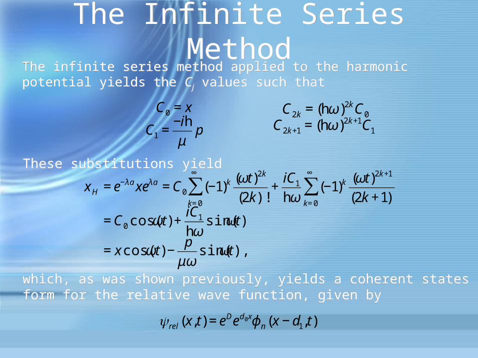
The Infinite Series MethodThe Infinite Series MethodThe infinite series method applied to the harmonic potential yields the Cj values such thatThe infinite series method applied to the harmonic potential yields the Cj values such that

These substitutions yield These substitutions yield

€

C0 = x

C1 =−ih

μp

which, as was shown previously, yields a coherent states form for the relative wave function, given bywhich, as was shown previously, yields a coherent states form for the relative wave function, given by

€

xH = e−λa xeλa = C0 (−1)k (ωt)2k

(2k)!k= 0

∞

∑ +iC1

hω(−1)k (ωt)2k +1

(2k +1)!k= 0

∞

∑

= C0 cos(ωt) +iC1

hωsin(ωt)

= x cos(ωt) −p

μωsin(ωt),

€

ψrel (x, t) = eDed 0xϕ n (x − d1, t).

€

C2k = (hω)2k C0

C2k +1 = (hω)2k +1C1.

In Conclusion …In Conclusion …• The model of two masses interacting in a harmonic potential and

subject to any time-limited force produces coherent states. Exceptin the case where the force goes to zero when the oscillator is in its equilibrium position with zero velocity.

• The wave function of this model is the product of a center of mass wave function and a relative motion wave function.

• The model of two masses interacting in a harmonic potential and subject to any time-limited force produces coherent states. Exceptin the case where the force goes to zero when the oscillator is in its equilibrium position with zero velocity.

• The wave function of this model is the product of a center of mass wave function and a relative motion wave function.

• We developed two methods of analyzing the similar model of a delta-kicked oscillator with a general potential. We found that this model will not produce the displacement-operator definition of coherent states.

• However, our new methods agree that the model with the harmonic potential does indeed yield coherent states.

• We developed two methods of analyzing the similar model of a delta-kicked oscillator with a general potential. We found that this model will not produce the displacement-operator definition of coherent states.

• However, our new methods agree that the model with the harmonic potential does indeed yield coherent states.